Citation: Montoya, O.D.;

Rivas-Trujillo, E.; Giral-Ramírez, D.A.

Selection and Location of Fixed-Step

Capacitor Banks in Distribution

Grids for Minimization of Annual

Operating Costs: A Two-Stage

Approach. Computers 2022, 11, 105.

https://doi.org/10.3390/

computers11070105

Academic Editors: Pedro Pereira,

Luis Gomes and João Goes

Received: 19 April 2022

Accepted: 20 June 2022

Published: 27 June 2022

Publisher’s Note: MDPI stays neutral

with regard to jurisdictional claims in

published maps and institutional affil-

iations.

Copyright: © 2022 by the authors.

Licensee MDPI, Basel, Switzerland.

This article is an open access article

distributed under the terms and

conditions of the Creative Commons

Attribution (CC BY) license (https://

creativecommons.org/licenses/by/

4.0/).

computers

Article

Selection and Location of Fixed-Step Capacitor Banks inDistribution Grids for Minimization of Annual OperatingCosts: A Two-Stage ApproachOscar Danilo Montoya 1,2,* , Edwin Rivas-Trujillo 1 and Diego Armando Giral-Ramírez 3

1 Grupo de Compatibilidad e Interferencia Electromágnetica, Facultad de Ingeniería, Universidad DistritalFrancisco José de Caldas, Bogotá 110231, Colombia; erivas@udistrital.edu.co

2 Laboratorio Inteligente de Energía, Facultad de Ingeniería, Universidad Tecnológica de Bolívar,Cartagena 131001, Colombia

3 Facultad Tecnológica, Universidad Distrital Francisco José de Caldas, Bogotá 110231, Colombia;dagiralr@udistrital.edu.co

* Correspondence: odmontoyag@udistrital.edu.co

Abstract: The problem regarding the optimal location and sizing of fixed-step capacitor banks indistribution networks with radial configuration is studied in this research by applying a two-stageoptimization approach. The first stage consists of determining the nodes where the capacitor bankswill be placed. In this stage, the exact mixed-integer nonlinear programming (MINLP) model thatrepresents the studied problem is transformed into a mixed-integer quadratic convex (MIQC) model.The solution of the MIQC model ensures that the global optimum is reached given the convexityof the solution space for each combination of nodes where the capacitor banks will be installed.With the solution of the MIQC, the suitable nodes for the installation of the fixed-step capacitorsare fixed, and their sizes are recursively evaluated in a power flow methodology that allows fordetermining the optimal sizes. In the second stage, the successive approximation power flow methodis applied to determine the optimal sizes assigned to these compensation devices. Numerical resultsin three test feeders with 33, 69, and 85 buses demonstrate the effectiveness of the proposed two-stage solution method for two operation scenarios: (i) operation of the distribution system underpeak load conditions throughout the year, and (ii) operation considering daily demand variationsand renewable generation penetration. Comparative results with the GAMS software confirm theexcellent results reached using the proposed optimization approach. All the simulations were carriedout in the MATLAB programming environment, version 2021b, as well as using the Gurobi solver inthe convex programming tool known as CVX.

Keywords: fixed-step capacitor banks; daily load variations; annual operating cost minimization;two-stage optimization approach; successive approximation power flow method

1. Introduction1.1. General Context

Electricity services have become public around the world, as they are considerednecessary for social development in both rural and urban areas [1]. To provide electricity toall end users (industrial, residential, and commercial), distribution networks are used whichare operated at medium- and low-voltage levels, most of which have radial structures [2].Radial configuration means that a distribution grid composed of n nodes has n− 1 lines,which allow for connecting all the end users to the substation by only one route [3,4]. Radialconfigurations are preferred in this context for two main reasons: (i) a radial configurationrepresents fewer kilometers in conductors and less electrical infrastructure (i.e., minimuminvestment costs) [5], and (ii) it reduces the complexity regarding the coordination issues ofprotective devices [6]. Even though these are strong, justifiable advantages for distribution

Computers 2022, 11, 105. https://doi.org/10.3390/computers11070105 https://www.mdpi.com/journal/computers

Computers 2022, 11, 105 2 of 19

companies, it is widely known that the radial configuration of the distribution networksincreases the operating costs of the grid (i.e., the costs of the energy losses) in comparisonwith any weakly meshed distribution topology [7].

1.2. Motivation

Due to the increment in grid power and energy losses caused by the radial topologybuilt into medium- and low-voltage distribution grids, distribution companies have im-plemented different alternatives to reduce their costs. These companies typically employthree main approaches to reduce grid power losses: (i) implementing grid reconfigurationschemes [8]; (ii) optimally siting and sizing dispersed generation and battery energy storagesystems [9]; (iii) optimally siting and sizing reactive power compensators [7]. All of thesemethodologies can have positive impacts on the total grid power losses. However, in thecase of the reconfiguration of distribution systems, it is necessary for distribution compa-nies to construct new distribution lines (tie lines) in order to redefine the grid topologybased on the current demand state of the network [10]. The installation of new lines maynot be an economical task, and the reconfiguration problem is highly dependent on thedemand behavior, which implies that an optimal solution for a particular load scenariomay not be optimal for other load scenarios [11]. In the case of the optimal placement andsizing of dispersed generation and energy storage systems, the aforementioned devicescan help with reducing energy losses in the distribution network [12]. However, their mainapplication is in the reduction of the greenhouse gas emissions in rural areas, as well asthat of energy purchasing costs at the substation bus. In addition, energy losses for theseapplications can sometimes increase, which are compensated by the use of renewables [13].The main goal of installing renewable energy resources and batteries is minimizing theannual grid operating costs of the network, including investments and maintenance costs,where energy losses are typically not considered to be part of the objective function [14].As for reactive power compensation, two main devices are used: (i) capacitor banks and(ii) distribution static compensators. The former are economical and have a long usefullife as well as minimum maintenance requirements. The latter also have a long useful life,as well as the ability to dynamically compensate reactive power. However, they are moreexpensive in comparison with with capacitor banks, and they are less reliable, since theseare composed of power electronic converters and require specialized control techniquesand communication channels [15].

Considering the above, this research aims to propose a new optimization methodologythat allows for minimizing the energy loss costs for distribution companies using fixed-stepcapacitor banks. Given that they are the most economical devices for reducing energylosses, they are well-recognized in the electrical sector, and they have long useful lives,regardless of the weather conditions, which implies that they can work correctly in areaswith complex climatic conditions.

1.3. State of the Art

The problem concerning the optimal location and sizing of capacitor banks in electricaldistribution networks is a well-known optimization problem for distribution grids. Here,we present a review of some contributions that employ metaheuristics and exact solutionmethods in order to deal with this optimization problem.

The authors of the ref. [16] suggested applying the simulated annealing algorithmto locate and size capacitor banks in radial distribution networks. The authors improvedthe effectiveness of the studied algorithm by using sensitivity factors in order to reducethe solution space, and their contribution was the inclusion of a duration curve for thesystem demand behavior. Numerical results in 9- and 69-node test feeders confirmed theapplicability of the proposed methodology regarding the minimization of the objectivefunction, which was associated with the annual energy losses and investment costs. Theauthors of the ref. [17] applied the flower pollination algorithm to locate and size capacitorbanks in distribution networks while considering loss density factors in order to reduce

Computers 2022, 11, 105 3 of 19

the dimension of the solution space. The numerical results obtained from test feeders com-posed of 15, 69, and 118 nodes demonstrate the effectiveness of the proposed algorithmsin comparison with literature reports based on metaheuristics. The authors focused onminimizing the annual grid operating costs while including the investment costs of thecapacitor banks. However, only the peak load scenario was tested, which can oversize thecapacitors when compared with daily load scenarios and also yield unrealistic reductioncosts. The authors of the ref. [18] used the Chu and Beasley genetic algorithm to determinethe location and size of fixed-step capacitor banks in distribution networks. The maincontribution of this work has to do with the application of this methodology to radial andmeshed distribution configurations without changing the power flow solver. Numericalresults demonstrated the effectiveness of the proposed optimization approach when com-pared to the solution of the exact model in GAMS (general algebraic modeling system) andliterature reports based on metaheuristics. The authors of the ref. [19] improved the flowerpollination algorithm employed by [17] to allocate and size fixed-step capacitor banks indistribution grids. Computational validations in four test feeders composed of 33, 34, 69,and 85 buses demonstrated the effectiveness of this algorithm when compared to fuzzylogic and genetic algorithms. However, the authors only considered peak-load operationconditions, which, as previously mentioned, produces capacitor oversizing and unrealisticpredictions regarding economic benefits.

The authors of the ref. [20] suggested the application of a discrete version of the vortexsearch algorithm to locate and size fixed-step capacitor banks in distribution grids withradial topology. Numerical results in the IEEE 33 and IEEE 69 grids demonstrate the effec-tiveness of this proposed algorithm in contrast with the flower pollination algorithm andthe solution of the exact model in the GAMS software. The authors of the ref. [5] applieda specialized version of the genetic algorithm to locate and size capacitor banks, voltageregulators, and dispersed generators in distribution networks in order to reduce energy losscosts and improve voltage profiles across the distribution grid. Numerical results demon-strated the effectiveness of this version of the genetic algorithm in comparison with tabusearch algorithms and particle swarm optimization methods. The authors of the ref. [21]proposed the application of the second-order cone programming with mixed-integer vari-ables for siting and sizing fixed-step capacitor banks in radial distribution networks toreduce grid power losses under peak load conditions. Numerical simulations includingannual grid operating costs under peak load conditions while considering investment costsin capacitor banks showed the effectiveness of the proposed methodology when comparedto the exact solution in the GAMS software and some metaheuristic optimizers. The authorsof the ref. [22] applied the classical genetic algorithm to locate and size capacitor banks indistribution networks. The main contribution of the authors corresponds to the usage of areal distribution network considering daily load and generation curves in order to ensurethat the numerical results reached by the genetic algorithm reflected the operational realityof the network.

Additional solution methodologies to address the problem concerning the optimallocation and sizing of capacitor banks in distribution grids are summarized in Table 1.

Table 1. Some recent literature approaches to locating and sizing capacitor banks in distribution networks.

Solution Methodology Objective Function Year Ref.

Bacterial foraging algorithmcombined with fuzzy logic Expected annual energy loss costs 2011 [23]

Modified honey bee matingoptimization

evolutionary algorithm

Minimizing power losses andimproving the voltage profile aswell as annual investment and

operating costs

2013 [24]

Cuckoo search-based algorithm Annual investment andoperating costs 2013, 2018 [25,26]

Computers 2022, 11, 105 4 of 19

Table 1. Cont.

Solution Methodology Objective Function Year Ref.

Artificial bee colonyoptimization algorithm

Annual investment andoperating costs 2014 [27]

Big bang/big crunch algorithmand fuzzy logic

Minimizing power losses,improving the voltage profile, and

reducing the gridvoltage imbalance

2016 [28]

Flower pollination algorithm Annual investment andoperating costs 2016, 2018 [17,19]

Salp swarm optimization Power loss minimization andvoltage profile improvement 2019 [29]

Recursive power flow evaluationsand loss sensitive factors

Power loss minimization andvoltage profile improvement 2020 [30]

Chu and Beasley and specializedgenetic algorithms

Annual investment andoperating costs 2020, 2021 [5,18]

Particle swarm optimization Annual investment andoperating costs 2022 [31]

Bat optimization algorithm Minimization of power loss 2022 [32]

Modified particle swarmoptimization method

Annual investment andoperating costs 2022 [31]

The most important characteristic of all the combinatorial optimization algorithmsreported in Table 1 is that all of the algorithms work under a leader–follower concept(also known as the master–slave concept), where the leader algorithm is a heuristic ormetaheuristic algorithm that defines the places or nodes where the capacitor banks will beinstalled, as well as their size. On the other hand, the follower corresponds to a power flowtool that allows for determining the final objective function values. The leader–followeroptimization approach allows for decoupling the discrete optimization problem fromthat of the nonlinear power flow, which allows for exploring and exploiting the solutionspace through penalty factors, with excellent numerical results as reported in [32] for fivedifferent metaheuristic optimization methods compared regarding the problem of theoptimal placement and sizing of capacitor banks for distribution system applications.

An additional characteristic of the methodologies listed in Table 1 is the use of objectivefunctions related to power loss minimization, voltage profile improvements, and annualinvestment and operating cost minimization, which shows that, for distribution companies,the most important aspect when fixed-step capacitor banks are integrated into their gridscorresponds to the economical feasibility of the final solution, including technical aspectsthat are economically quantifiable, as is the case for energy losses, as well as ensuring goodvoltage performances.

1.4. Contribution and Scope

Considering the most common aspects to be addressed regarding the problem of theoptimal placement and sizing fixed-step capacitor banks in distribution networks, that is,annual investment and operating costs reduction and the use of master–slave optimizationstrategies, this research contributes with the following aspects:

i. It presents a two-stage optimization methodology to solve the studied problem, whichseparates the location problem from the power flow (sizing) problem. As for thelocation problem, this work proposes the use of a reduced mixed-integer quadraticconvex (MIQC) formulation based on the optimal branch power flow formulationpresented in [33]. This MIQC formulation allows for simplifying the exact MINLPmodel, and it defines the nodes for the installation of the fixed-step capacitor banks.

Computers 2022, 11, 105 5 of 19

ii. It determines the optimal sizes of the fixed-step capacitor banks in the slave stageby presenting a recursive-based power flow solution method that, once the nodeswhere the capacitor banks will be installed are defined, evaluates all the discretepossibilities for the capacitor sizes. The power flow tool used to evaluate the capacitorsizes corresponds to the triangular-based power flow method that is specialized forradial distribution system topologies [34].

It is worth mentioning that the MIQC part of the proposed two-stage optimizationmethod has been previously proposed in [35] to address the problem concerning theoptimal installation of solar photovoltaic generators. However, the recursive power flowsolution to determine the optimal sizes of the capacitor banks has not been previouslyimplemented. In addition, the proposed optimization method is only designed for strictlyradial distribution networks due to the restrictions of the MIQC formulation regarding thebranch convex power flow presented in [36].

1.5. Document Organization

The remainder of this work has the following structure: Section 2 presents the MIQCformulation to select the set of nodes where the fixed-step capacitor banks are to be installed;Section 3 shows the application of the recursive power flow solution method; Section 4presents a summary of the proposed two-stage optimization methodology; Section 5 revealsthe main characteristics of the test feeders, the daily load behavior, and the characterizationof the objective function calculation; Section 6 presents the numerical results obtainedwith the proposed two-stage optimization approach and their comparison with literaturereports; finally, Section 7 presents the conclusions drawn from this research.

2. Selection of the Nodes

This section presents the approximate mixed-integer quadratic convex (MIQC) modelfor the placement of the fixed-step capacitor banks. The MIQC model corresponds tothe relaxation of the branch power flow model proposed in [33] to reconfigure radialdistribution grids. The main characteristics of this formulation are as follows: (i) the voltagemagnitudes are assumed close to the unity value in a per-unit representation, and (ii) activeand reactive power losses in distribution lines can be neglected due to the fact that thepower flows are larger in comparison. The approximated MIQC model to select the nodeswhere the capacitor banks will be assigned is defined in Equations (1)–(5) [37].

Objective function:

min zapprox = CkWhT ∑ij∈L

∑h∈H

Rij

(p2

ij,h + q2ij,h

)∆h + ∑

j∈N∑c∈C

Ccapc Qcxjc (1)

Subject to:

pij,h − ∑k:(jk)∈L

pjk,h = Pdj,h, ∀j ∈ N , j 6= slack, ∀h ∈ H, (2)

qij,h − ∑k:(jk)∈L

qjk,h = Qdj,h − ∑

c∈CQcxjc, ∀j ∈ N , j 6= slack, ∀h ∈ H, (3)

∑c∈C

xjc ≤ 1, ∀j ∈ N , j 6= slack, (4)

∑j∈N

∑c∈C

xjc ≤ Ncapava , ∀j ∈ N , j 6= slack. (5)

where min zapprox corresponds to the value of the objective function value containing theexpected annual grid operating costs of the network, which combines the annual costsof the energy losses with the investment costs for the fixed-step capacitor banks; CkWhrepresents the expected average costs of the energy losses; T is the number of days in ayear; Rij is the resistive parameter associated with the distribution line that connects node iwith node j; pij,h (qij,h) corresponds to the active (reactive) power flow sent from nodes i to

Computers 2022, 11, 105 6 of 19

j for each period of time h; pjk,h and qjk,h represent the active and reactive power flows sentfrom node j to node k for the period of time h, respectively; Pd

j,h and Qdj,h are the active and

reactive power demands at node j for each period of time h; Ccapc represents the cost of a

type c fixed-step capacitor bank; Qc represents the nominal reactive power rate of a type cfixed-step capacitor bank; xjc is the binary decision variable that defines whether the typec fixed-step capacitor bank is located at node j (xjc = 1) or not (xjc = 0); and Ncap

ava is aninteger parameter that defines the number of fixed-step capacitor banks that can be addedto the network. Note that N represents the set containing all the nodes of the network, andH is the set with all the periods of time included in the planning study.

The proposed MIQC model presented in Equations (1)–(5) can be interpreted asfollows: Equation (1) presents an approximate objective function that evaluates the totalinvestment costs of the fixed-step capacitor banks, with an estimation of the expectedenergy loss costs (note that the estimation of the power losses was initially introducedin [33]); Equations (2) and (3) represent the approximation of the active and reactive powerflow variables in the system when it has been assumed that the voltages are ideal; inequalityconstraints (Equations (4) and (5)) define that it is only possible to locate a maximum of onefixed-step capacitor bank per node, and that the number of banks available for installationis a maximum of Ncap

ava .

Remark 1. It is important to emphasize that the MIQC presented from Equation (1) to Equation (5)yields the set of nodes where the fixed-step capacitor banks will be installed, as well as their expectedsizes [37]. However, the solution regarding the sizes corresponds to an approximate solution dueto the simplification of the exact MINLP model. For this reason, these sizes are defined in the nextstep of the solution methodology through the recursive solution of multiple power flows for eachfixed-step size combination.

On the other hand, it is worth mentioning that the proposed MIQC model defined inEquations (1)–(5) differs from the optimization model presented in [33] in two main respects:(i) our proposed model deals with reactive power compensation by means of the optimalinstallation of fixed-step capacitor banks in distribution networks while considering dailyload curves, whereas the MIQC model in [33] was developed to solve the problem ofoptimal reconfiguration in radial distribution networks while considering the peak loadoperation scenario; and (ii) our optimization model is focused on the determination of theannual expected operating costs of the network, whereas the model proposed in [33] onlyfocuses on the minimization of the power losses, without considering the intrinsic cost ofopening and closing tie lines to reconfigure the distribution network.

3. Assigning the Optimal Sizes

This optimization stage aims to determine the optimal sizes of the fixed-step capacitorbanks once the MIQC model has defined all the nodes where they are to be installed, i.e.,the value of the variable xjc. To this effect, a recursive power flow solution approach isconsidered which is based on the well-known successive approximation method proposedby [38]. The recursive power flow approach evaluates each possible capacitor size availablefor the j nodes provided by the first optimization stage.

To illustrate the application of the recursive power flow formula to each possiblecapacitor size combination, the solution vector defined in Equation (6) is used.

ysol = [i, j, k, | 3, 9, c], (6)

where ysol is the solution vector that determines the sizes of the capacitors placed in nodesi, j, and k. The most important characteristic of the solution vector in Equation (6) is that itallows for easily calculating the total investment costs of the fixed-step capacitor banks (seesecond component of the objective function defined in Equation (1)).

Computers 2022, 11, 105 7 of 19

It is important to mention that, for the studied grids, the number of capacitors availablefor installations is three (i.e., Ncap

ava = 3), and the number of capacitor sizes available is 14(c = 14). This implies that the dimension of the solution space regarding the sizes of thecapacitors is 143, which corresponds to 2774 possible combinations [37]. Note that thisdimension of the solution space is small, and it can be easily and exhaustively revised withthe proposed recursive power flow evaluation method.

To evaluate each solution vector ysol, a new vector in the recursive power flow for-mulation is considered: Scap,h. The purpose of Scap,h is to add the sizes defined for thecapacitor in the solution vector (see Equation (6) to the power flow problem. This vector isdefined in Equation (7). Si,h

Sj,hSk,h

=

jQ3jQ9jQc

, (7)

With the auxiliary vector defined in Equation (6), the successive approximation powerflow formula proposed in [38] is modified, which takes the form presented in Equation (8).

Vm+1d,h = Y−1

dd

[diag−1

(Vm

d,h

)(S?cap,h − S?d,h

)−YdsVs,h

]. (8)

All of the components of the power flow Formula (8) can be consulted in [39].Note that the selection of the successive approximation power flow method defined

by Equation (8) is motivated by two main aspects: (i) its convergence can be ensured withthe application of the Banach fixed-point theorem [40]; and (ii) it can be used for radial andmeshed distribution networks with no changes to its formulation [39]. The second aspect isvery important since it allows for extending the proposed two-stage solution methodologyto meshed configurations with no change regarding the radial operation scenario.

To define the stopping criterion of the recursive power flow Formula (8), the differencebetween two consecutive solutions at the iterations m and m + 1 is used. This stoppingcriterion is defined in Equation (9).

maxh

||Vm+1

d,h | − |Vmd,h||

≤ ε, (9)

where ε is the tolerance value, which is assigned as 1× 10−10, as recommended in [38].Now, with the solution of the power flow problem through the application of Equation (8),

the total grid power losses of the network can be calculated for each period of time, as definedin Equation (10):

Ploss,h = realV>h (YbusVh)

?

, (10)

whereVh is the vector containing the substation and demand voltages ordered as [Vs,h Vd,h]>,

and Ybus is the distribution network’s nodal admittance matrix. With the power losses foreach period of time, the exact operating costs of the distribution systems with fixed-stepcapacitor banks, that is, min zcosts, can obtained as defined in Equation (11).

min zcosts = CkWhT ∑ij∈L

∑h∈H

Ploss,h∆h + ∑j∈N

∑c∈C

Ccapc Qcxjc (11)

4. Summary of the Solution Methodology

The two-stage solution methodology proposed in this research for locating and sizingfixed-step capacitor banks in radial distribution networks is summarized in Algorithm 1.

Computers 2022, 11, 105 8 of 19

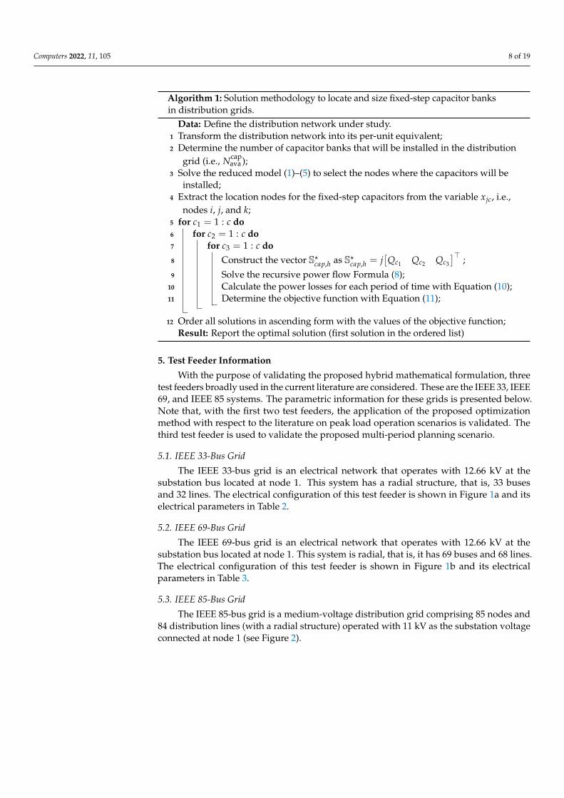
Algorithm 1: Solution methodology to locate and size fixed-step capacitor banksin distribution grids.

Data: Define the distribution network under study.1 Transform the distribution network into its per-unit equivalent;2 Determine the number of capacitor banks that will be installed in the distribution

grid (i.e., Ncapava );

3 Solve the reduced model (1)–(5) to select the nodes where the capacitors will beinstalled;

4 Extract the location nodes for the fixed-step capacitors from the variable xjc, i.e.,nodes i, j, and k;

5 for c1 = 1 : c do6 for c2 = 1 : c do7 for c3 = 1 : c do8 Construct the vector S?cap,h as S?cap,h = j

[Qc1 Qc2 Qc3

]> ;

9 Solve the recursive power flow Formula (8);10 Calculate the power losses for each period of time with Equation (10);11 Determine the objective function with Equation (11);

12 Order all solutions in ascending form with the values of the objective function;Result: Report the optimal solution (first solution in the ordered list)

5. Test Feeder Information

With the purpose of validating the proposed hybrid mathematical formulation, threetest feeders broadly used in the current literature are considered. These are the IEEE 33, IEEE69, and IEEE 85 systems. The parametric information for these grids is presented below.Note that, with the first two test feeders, the application of the proposed optimizationmethod with respect to the literature on peak load operation scenarios is validated. Thethird test feeder is used to validate the proposed multi-period planning scenario.

5.1. IEEE 33-Bus Grid

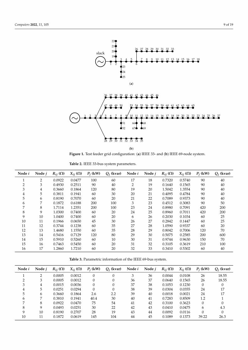
The IEEE 33-bus grid is an electrical network that operates with 12.66 kV at thesubstation bus located at node 1. This system has a radial structure, that is, 33 busesand 32 lines. The electrical configuration of this test feeder is shown in Figure 1a and itselectrical parameters in Table 2.

5.2. IEEE 69-Bus Grid

The IEEE 69-bus grid is an electrical network that operates with 12.66 kV at thesubstation bus located at node 1. This system is radial, that is, it has 69 buses and 68 lines.The electrical configuration of this test feeder is shown in Figure 1b and its electricalparameters in Table 3.

5.3. IEEE 85-Bus Grid

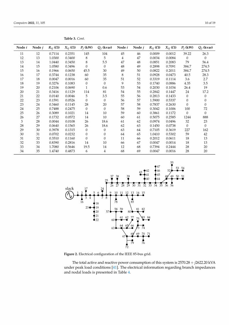
The IEEE 85-bus grid is a medium-voltage distribution grid comprising 85 nodes and84 distribution lines (with a radial structure) operated with 11 kV as the substation voltageconnected at node 1 (see Figure 2).

Computers 2022, 11, 105 9 of 19

∼slack

1 2

3 4 5

6

7 8 9 10 11 12 13 14 15 16 17 18

23

24

25

19

20

21

22

26 27 28 29 30 31 32 33

(a)

∼ 1 2 3 4 5 6 7 8 9 10 11 12 13 14 15 16 17 18 19 20 21 22 23 24 25 26 27

36 37 38 39 40 41 42 43 44 45 46

47 48 49 50 53 54 55 56 57 58 59 60 61 62 63 64 65

51

52

66

67

68

69

28 29 30 31 32 33 34 35

(b)

Figure 1. Test feeder grid configuration: (a) IEEE 33- and (b) IEEE 69-node system.

Table 2. IEEE 33-bus system parameters.

Node i Node j Rij (Ω) Xij (Ω) Pj (kW) Qj (kvar) Node i Node j Rij (Ω) Xij (Ω) Pj (kW) Qj (kvar)

1 2 0.0922 0.0477 100 60 17 18 0.7320 0.5740 90 402 3 0.4930 0.2511 90 40 2 19 0.1640 0.1565 90 403 4 0.3660 0.1864 120 80 19 20 1.5042 1.3554 90 404 5 0.3811 0.1941 60 30 20 21 0.4095 0.4784 90 405 6 0.8190 0.7070 60 20 21 22 0.7089 0.9373 90 406 7 0.1872 0.6188 200 100 3 23 0.4512 0.3083 90 507 8 1.7114 1.2351 200 100 23 24 0.8980 0.7091 420 2008 9 1.0300 0.7400 60 20 24 25 0.8960 0.7011 420 2009 10 1.0400 0.7400 60 20 6 26 0.2030 0.1034 60 2510 11 0.1966 0.0650 45 30 26 27 0.2842 0.1447 60 2511 12 0.3744 0.1238 60 35 27 28 1.0590 0.9337 60 2012 13 1.4680 1.1550 60 35 28 29 0.8042 0.7006 120 7013 14 0.5416 0.7129 120 80 29 30 0.5075 0.2585 200 60014 15 0.5910 0.5260 60 10 30 31 0.9744 0.9630 150 7015 16 0.7463 0.5450 60 20 31 32 0.3105 0.3619 210 10016 17 1.2860 1.7210 60 20 32 33 0.3410 0.5302 60 40

Table 3. Parametric information of the IEEE 69-bus system.

Node i Node j Rij (Ω) Xij (Ω) Pj (kW) Qj (kvar) Node i Node j Rij (Ω) Xij (Ω) Pj (kW) Qj (kvar)

1 2 0.0005 0.0012 0 0 3 36 0.0044 0.0108 26 18.552 3 0.0005 0.0012 0 0 36 37 0.0640 0.1565 26 18.553 4 0.0015 0.0036 0 0 37 38 0.1053 0.1230 0 04 5 0.0251 0.0294 0 0 38 39 0.0304 0.0355 24 175 6 0.3660 0.1864 2.6 2.2 39 40 0.0018 0.0021 24 176 7 0.3810 0.1941 40.4 30 40 41 0.7283 0.8509 1.2 17 8 0.0922 0.0470 75 54 41 42 0.3100 0.3623 0 08 9 0.0493 0.0251 30 22 42 43 0.0410 0.0475 6 4.39 10 0.8190 0.2707 28 19 43 44 0.0092 0.0116 0 010 11 0.1872 0.0619 145 104 44 45 0.1089 0.1373 39.22 26.3

Computers 2022, 11, 105 10 of 19

Table 3. Cont.

Node i Node j Rij (Ω) Xij (Ω) Pj (kW) Qj (kvar) Node i Node j Rij (Ω) Xij (Ω) Pj (kW) Qj (kvar)

11 12 0.7114 0.2351 145 104 45 46 0.0009 0.0012 39.22 26.312 13 1.0300 0.3400 8 5 4 47 0.0034 0.0084 0 013 14 1.0440 0.3450 8 5.5 47 48 0.0851 0.2083 79 56.414 15 1.0580 0.3496 0 0 48 49 0.2898 0.7091 384.7 274.515 16 0.1966 0.0650 45.5 30 49 50 0.0822 0.2011 384.7 274.516 17 0.3744 0.1238 60 35 8 51 0.0928 0.0473 40.5 28.317 18 0.0047 0.0016 60 35 51 52 0.3319 0.1114 3.6 2.718 19 0.3276 0.1083 0 0 9 53 0.1740 0.0886 4.35 3.519 20 0.2106 0.0690 1 0.6 53 54 0.2030 0.1034 26.4 1920 21 0.3416 0.1129 114 81 54 55 0.2842 0.1447 24 17.221 22 0.0140 0.0046 5 3.5 55 56 0.2813 0.1433 0 022 23 0.1591 0.0526 0 0 56 57 1.5900 0.5337 0 023 24 0.3460 0.1145 28 20 57 58 0.7837 0.2630 0 024 25 0.7488 0.2475 0 0 58 59 0.3042 0.1006 100 7225 26 0.3089 0.1021 14 10 59 60 0.3861 0.1172 0 026 27 0.1732 0.0572 14 10 60 61 0.5075 0.2585 1244 8883 28 0.0044 0.0108 26 18.6 61 62 0.0974 0.0496 32 2328 29 0.0640 0.1565 26 18.6 62 63 0.1450 0.0738 0 029 30 0.3978 0.1315 0 0 63 64 0.7105 0.3619 227 16230 31 0.0702 0.0232 0 0 64 65 1.0410 0.5302 59 4231 32 0.3510 0.1160 0 0 11 66 0.2012 0.0611 18 1332 33 0.8390 0.2816 14 10 66 67 0.0047 0.0014 18 1333 34 1.7080 0.5646 19.5 14 12 68 0.7394 0.2444 28 2034 35 1.4740 0.4873 6 4 68 69 0.0047 0.0016 28 20

slack1 2

3 4

5 6

7 8

9 10 11 12 13 14 15

16

17

1819202122

23

24

25

26 27 28 29 30 31 32 33 34 35 36

37 38 3940414243

44454647

48 49 50 51

5253 54

55

56

5758 59

6061 62

6364 65 66

6768 69 70 71

72

73 74

75

76

77

78

79

8081 82

83 84

85

Figure 2. Electrical configuration of the IEEE 85-bus grid.

The total active and reactive power consumption of this system is 2570.28+ j2622.20 kVAunder peak load conditions [41]. The electrical information regarding branch impedancesand nodal loads is presented in Table 4.

Computers 2022, 11, 105 11 of 19

Table 4. Parametric information of the IEEE 85-bus system.

Node i Node j Rij (Ω) Xij (Ω) Pj (kW) Qj (kvar) Node i Node j Rij (Ω) Xij (Ω) Pj (kW) Qj (kvar)

1 2 0.108 0.075 0 0 34 44 1.002 0.416 35.28 35.992 3 0.163 0.112 0 0 44 45 0.911 0.378 35.28 35.993 4 0.217 0.149 56 57.13 45 46 0.911 0.378 35.28 35.994 5 0.108 0.074 0 0 46 47 0.546 0.226 14 14.285 6 0.435 0.298 35.28 35.99 35 48 0.637 0.264 0 06 7 0.272 0.186 0 0 48 49 0.182 0.075 0 07 8 1.197 0.820 35.28 35.99 49 50 0.364 0.151 36.28 37.018 9 0.108 0.074 0 0 50 51 0.455 0.189 56 57.139 10 0.598 0.410 0 0 48 52 1.366 0.567 0 010 11 0.544 0.373 56 57.13 52 53 0.455 0.189 35.28 35.9911 12 0.544 0.373 0 0 53 54 0.546 0.226 56 57.1312 13 0.598 0.410 0 0 52 55 0.546 0.226 56 57.1313 14 0.272 0.186 35.28 35.99 49 56 0.546 0.226 14 14.2814 15 0.326 0.223 35.28 35.99 9 57 0.273 0.113 56 57.132 16 0.728 0.302 35.28 35.99 57 58 0.819 0.340 0 03 17 0.455 0.189 112 114.26 58 59 0.182 0.075 56 57.135 18 0.820 0.340 56 57.13 58 60 0.546 0.226 56 57.1318 19 0.637 0.264 56 57.13 60 61 0.728 0.302 56 57.1319 20 0.455 0.189 35.28 35.99 61 62 1.002 0.415 56 57.1320 21 0.819 0.340 35.28 35.99 60 63 0.182 0.075 14 14.2821 22 1.548 0.642 35.28 35.99 63 64 0.728 0.302 0 019 23 0.182 0.075 56 57.13 64 65 0.182 0.075 0 07 24 0.910 0.378 35.28 35.99 65 66 0.182 0.075 56 57.138 25 0.455 0.189 35.28 35.99 64 67 0.455 0.189 0 025 26 0.364 0.151 56 57.13 67 68 0.910 0.378 0 026 27 0.546 0.226 0 0 68 69 1.092 0.453 56 57.1327 28 0.273 0.113 56 57.13 69 70 0.455 0.189 0 028 29 0.546 0.226 0 0 70 71 0.546 0.226 35.28 35.9929 30 0.546 0.226 35.28 35.99 67 72 0.182 0.075 56 57.1330 31 0.273 0.113 35.28 35.99 68 73 1.184 0.491 0 031 32 0.182 0.075 0 0 73 74 0.273 0.113 56 57.1332 33 0.182 0.075 14 14.28 73 75 1.002 0.416 35.28 35.9933 34 0.819 0.340 0 0 70 76 0.546 0.226 56 57.1334 35 0.637 0.264 0 0 65 77 0.091 0.037 14 14.2835 36 0.182 0.075 35.28 35.99 10 78 0.637 0.264 56 57.1326 37 0.364 0.151 56 57.13 67 79 0.546 0.226 35.28 35.9927 38 1.002 0.416 56 57.13 12 80 0.728 0.302 56 57.1329 39 0.546 0.226 56 57.13 80 81 0.364 0.151 0 032 40 0.455 0.189 35.28 35.99 81 82 0.091 0.037 56 57.1340 41 1.002 0.416 0 0 81 83 1.092 0.453 35.28 35.9941 42 0.273 0.113 35.28 35.99 83 84 1.002 0.416 14 14.2841 43 0.455 0.189 35.28 35.99 13 85 0.819 0.340 35.28 35.99

5.4. Economic Assessment Parameters

To determine the annual grid’s operating costs when fixed-step capacitor banks areinstalled, the information on their sizes and costs is shown in Table 5 (adapted from [19]).

Table 5. Costs of the capacitors according to their capacity.

Option Qc (kvar) Cost(USD/kvar-year) Option Qc (kvar) Cost

(USD/kvar-year)1 150 0.500 8 1200 0.1702 300 0.350 9 1350 0.2073 450 0.253 10 1500 0.2014 600 0.220 11 1650 0.1935 750 0.276 12 1800 0.8706 900 0.183 13 1950 0.2117 1050 0.228 14 2100 0.176

Computers 2022, 11, 105 12 of 19

6. Computational Implementation

The proposed two-stage optimization approach was implemented in version 2019b ofthe MATLAB software. The mixed-integer linear programming model was implementedusing CVX and the Gurobi solver. The recursive power flow solution was implementedby means of our own scripts using the successive approximation power flow formulation.All simulations were run on a desktop computer with an INTEL(R) Core(TM) i7− 77002.8-GHz CPU and 16.0 GB of RAM on a 64-bit version of Microsoft Windows 10. In the caseof the GAMS software, version 23.5 was used along with the BONMIN solver [42].

Note that, in order to calculate the percentage of improvement of the proposed two-stage optimization methodology with respect to the benchmark cases, the following expres-sion was used:

Imp% = 100%|zbc

cost| − |zcost|zbc

cost(12)

where Imp% represents the percentage of improvement with respect to the benchmark case,and zbc

cost is the operating cost of the network with no fixed-step capacitor banks installed(that is, benchmark simulation case).

6.1. Comparison with Literature Reports

To demonstrate that the proposed two-stage solution methodology is efficient in deter-mining the optimal siting of the fixed-step capacitor banks in radial distribution networks,here, our approach is compared with four different optimization methods reported in thecurrent literature when the objective function is to minimize the total grid power losses (seeTable 6). These methods are: the analytical method (AM) [43], the two-stage method (TSM),the hybrid fuzzy-based genetic algorithm (FRCGA) [44], GAMS [18], teaching-learningbased optimization [45], and the flower pollination algorithm (FPA) [19].

Numerical results in Table 6 show that the proposed two-stage optimization methodaddresses the problem of the optimal location and sizing of fixed-step capacitor banks indistribution systems with a high efficiency when compared with the literature reports. Notethat for both test feeders, the final location and sizes for the reactive power compensatorsreached with the MIQC model allow for better objective function vales when comparedwith the best report in [19]. In the case of the IEEE 33-bus grid, the proposed MIQCmodel reaches an objective function of 138.473 kW, which is 0.6020 kW better than the FPA,whereas in the IEEE 69-bus grid, this improvement is about 0.1880 kW with respect to theGAMS solution. Even though if this results represent small improvements with respect tothe literature reports, these confirm the effectiveness of the proposed model in dealing withthe minimization of the annual grid operating costs including fixed-step capacitor banksinto distribution networks with a radial configuration.

6.2. IEEE 33-Bus Grid

Regarding the IEEE 33-bus grid, it was considered that the system was operated underthe peak load conditions throughout the year, as recommended in [19]. The proposedMIQC model determined that the fixed-step capacitor banks should be located at nodes13, 24, and 30. Once these placements were fixed, in the second optimization stage, therecursive power flow evaluation defined that the optimal sizes for the fixed-step capacitorbanks were 450, 450, and 1050 kvar, respectively. Note that, if this solution is implemented,then the expected reduction compared to the benchmark case (USD/year 35, 445.909) isabout USD/year 11, 698.592, i.e., 33.04%. It is important to mention that, in order to reachthis solution in the IEEE 33-bus grid, it is only necessary to invest USD/year 467.10 inreactive power compensators. To demonstrate the effectiveness of the proposed MIQCmodel, Table 7 is presents the comparison between the first three solutions reached by ourtwo-stage solution proposal and the optimal solution found via the exact model in GAMS.Note that the solution reached using the proposed two-stage optimization method reduces

Computers 2022, 11, 105 13 of 19

the GAMS solution by about USD/year 111.9960, that is, 0.47 % of improvement of theMIQC model in comparison with the GAMS solution.

Table 6. Comparative results between the two-stage approach and multiple literature reports.

Method Size (Node) (Mvar) Losses (kW)IEEE 33-bus grid

Benc. Case - 210.987AM 0.45(9), 0.80(29), 0.90(30) 171.780TSM 0.85(7), 0.025(29), 0.90(30) 144.040FRCGA 0.475(6), 0.175(8), 0.35(9), 0.025(28), 0.30(29), 0.40(30) 141.240FPA 0.45(13), 0.45(24), 0.90(30) 139.075GAMS 0.30(14), 0.45(24), 1.05(30) 139.292

MIQC 0.45(13), 0.45(24), 1.05(30) 138.473IEEE 69-bus grid

Benc. Case - 225.072AM 0.90(11), 1.05(29), 0.45(60) 163.280TSM 0.225(19), 0.90(62), 0.225(63) 148.910TBLO 0.60(12), 1.05(61), 0.15(64) 146.350FPA 0.45(11), 0.15(22), 1.35(61) 145.860GAMS 0.45(11), 0.15(27), 1.20(61) 145.738

MIQC 0.45(11), 0.15(21), 1.20(61) 145.550

Table 7. Comparative results between the GAMS and the proposed MIQC proposal, IEEE 33-bus grid.

Method Size (Node) (Mvar) Losses (kW) C. Caps. USD C. Total USD

GAMS 0.30(14), 0.45(24),1.05(30) 139.292 458.25 23,859.313

MIQC (sol. 1) 0.45(13), 0.45(24),1.05(30) 138.473 467.10 23,747.317

MIQC (sol. 2) 0.45(13), 0.60(24),0.90(30) 138.917 410.55 23,748.531

MIQC (sol. 3) 0.45(13), 0.45(24),0.90(30) 139.075 392.40 23,757.083

The most interesting result in Table 7 is that, with slight modifications in the sizes ofthe capacitor banks at nodes 24 and 30 (variations of 150 kvar), solutions are found withjust 10 dollars of difference, all of them better than the solution found with GAMS.

One of the main results in Table 7 is that, with the proposed two-stage optimizationmethod, it is possible to list the alternative solutions. Note that, in this list, there are threesolutions with better final values regarding the final objective function than in the solutionyielded by GAMS.

6.3. IEEE 69-Bus Grid

In this test feeder, and considering a peak-load operation scenario as reported in [19],the solution of the MIQC model in the nodal selection stage identified nodes 11, 21, and 61as the optimal places to locate fixed-step capacitor banks. By fixing these nodal placementsfor the capacitors, in the refinement stage, the sizes found for the capacitors were 450,150, and 1200 kvar, respectively. With this solution, the yearly operating cost reductioncompared to the benchmark case (USD/year 37, 812.056) is about USD/year 12, 966.81,i.e., 34.29%. Note that this solution only requires an investment of USD/year 392.85 bythe distribution company. On the other hand, Table 8 presents the comparisons betweenthe solution reached using the GAMS software (exact MINLP solution) and the first foursolutions found using the proposed two-stage solution approach. Note that the solutionreached using the proposed two-stage optimization method reduces the GAMS solution byabout USD/year 31.6640, i.e., 0.13 % of improvement of the MIQC model with respect tothe GAMS solution.

Computers 2022, 11, 105 14 of 19

Table 8. Comparative results between GAMS and the MIQC proposal for the IEEE 69-bus test feeder.

Method Size (Node) (Mvar) Losses (kW) C. Caps. USD C. Total USD

GAMS 0.45(11), 0.15(27),1.20(61) 145.738 392.85 24,876.910

MIQC (sol. 1) 0.45(11), 0.15(21),1.20(61) 145.550 392.85 24,845.246

MIQC (sol. 2) 0.30(11), 0.30(21),1.20(61) 145.492 414.00 24,856.573

MIQC (sol. 3) 0.60(11), 0.15(21),1.20(61) 145.614 411.00 24,874.173

MIQC (sol. 4) 0.45(11), 0.30(21),1.20(61) 145.556 422.85 24,876.229

The results in Table 8 show that the proposed two-stage optimization approach pro-vides at least four solution methods with better numerical performance with respect to theobjective function when compared to the GAMS solution. In addition, as with the IEEE33-bus feeder, for this test system, it is observed that small variations (150 kvar) in somenodes yield solutions with expected reductions lower than 31 dollars per year of operation.

6.4. Numerical Results Considering Daily Load Variations

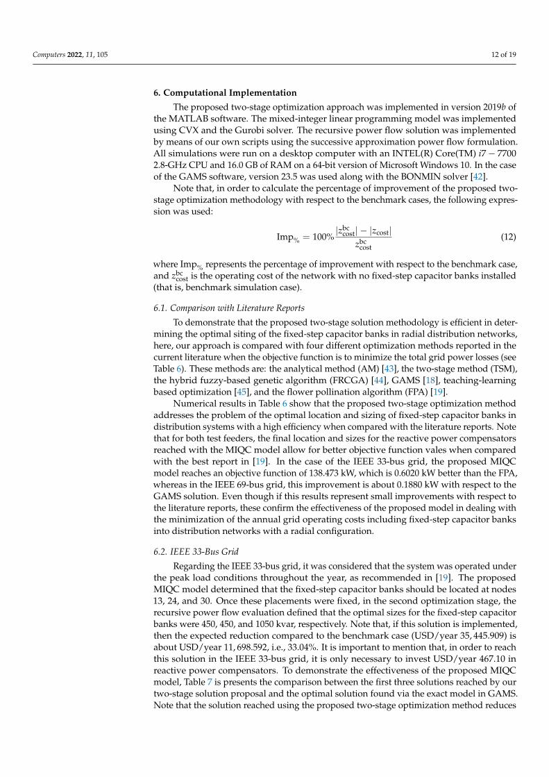
This subsection extends the analysis of the optimal placement of the fixed-step capaci-tor banks to daily operation scenarios while considering the presence of solar photovoltaic(PV) generation and daily load variations [13]. The demand load variations and the ex-pected solar PV generation are depicted in Figure 3.

1 2 3 4 5 6 7 8 9 10 11 12 13 14 15 16 17 18 19 20 21 22 23 240

0.10.20.30.40.50.60.70.80.9

1.01

Time (h)

Dem

and/

Sola

rcu

rves

(p.u

) Demand Solar

Figure 3. Expected behavior of the demand and PV generation for a typically sunny day.

In the case of PV generation, the optimal sizes reported in [13] for the IEEE 85-bus testfeeder are considered. These PV sources are located in nodes 35, 67, and 71, with sizes of1631.31, 463.33, and 503.80 kW, respectively.

In addition, two simulation scenarios are considered. The first case involves theoperation of the IEEE 85-bus grid while only considering the daily power demand withzero penetration of PV sources. The second case includes both curves, taking into accountthat the PV sources generate the maximum power available all the time.

6.4.1. Daily Operation without PV Generation

In this simulation case, the expected annual operating costs of the network withoutincluding fixed-step capacitor banks (i.e., the benchmark case) were USD/year 27, 924.793.Once the two-stage optimization methodology was applied to the IEEE 85-bus grid, thenodes found for placing the fixed-step capacitor banks were 9, 34, and 67. With theselocations, the annual expected operating costs of the network considering daily loadvariation were reduced to USD/year 16, 089.331, i.e., a reduction of 42.38%. The sizes ofthe capacitors were 600, 450, and 450 kvar, respectively, with an annual investment of

Computers 2022, 11, 105 15 of 19

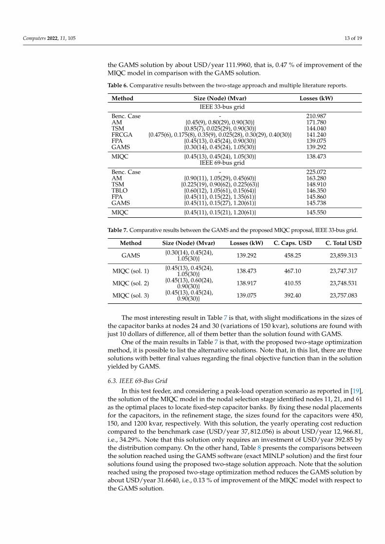
359.70 dollars. Figure 4 presents the daily behavior of the energy losses for one day in thissimulation scenario.

1 2 3 4 5 6 7 8 9 10 11 12 13 14 15 16 17 18 19 20 21 22 23 240

50

100

150

200

250

300

350

Time (h)

Pow

erlo

ss(k

W)

Without compensationWith compensation

Figure 4. Daily behavior of power losses without considering PV injection.

As expected, the results in Figure 4 show that the daily energy losses are reducedwhen the capacitor banks are installed in the distribution grid. For this simulation scenario,the daily energy losses are 3989.256 kWh/day when no capacitor banks are installed, andthese are reduced to 2247.090 kWh/day.

6.4.2. Daily Operation Including PV Generation

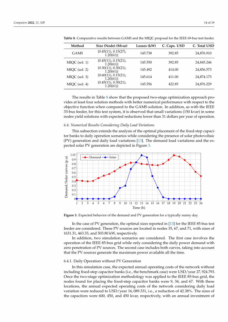
In this simulation scenario, the optimal location of fixed-step capacitor banks is evalu-ated while considering the PV generators to be active and with maximum power generation.The annual expected operating costs without integrating capacitor banks (i.e., the bench-mark case) was USD/year 21, 313.872. On the other hand, when the MIQC model wassolved, the nodes where the fixed-step capacitor banks were to be placed were 9, 34, and 67(note that these are the same nodes for the previous simulation scenario). Now, fixing thesenodes in the recursive power flow approach, the optimal sizes for these capacitors were 600,450, and 450 kvar (these sizes are also the same as those reached in the previous simulationscenario). With these sizes, the expected annual grid operating costs of the network arereduced to USD/year 10, 574.253, that is, a 50.39% reduction compared to the benchmarkcase. Note that, in order to reach this solution, the total investment in fixed-step capacitorbanks is 359.70 dollars. Figure 5 presents the daily behavior of the energy losses for oneday in this simulation scenario.

1 2 3 4 5 6 7 8 9 10 11 12 13 14 15 16 17 18 19 20 21 22 23 240

50

100

150

200

250

300

350

Time (h)

Pow

erlo

ss(k

W)

Without compensationWith compensation

Figure 5. Daily behavior of power losses considering PV injection.

As expected, the results in Figure 5 show that the daily energy losses are reducedwhen the capacitor banks are installed in the distribution grid. For this simulation scenario,

Computers 2022, 11, 105 16 of 19

the daily energy losses are 3044.839 kWh/day when no capacitor banks are installed, andthese are reduced to 1459.222 kWh/day.

6.4.3. Complementary Analysis

It is important to mention that, in the studied simulation cases for the IEEE 85-busgrid, it was observed that: (i) the presence of dispersed generation helps with the expectedcosts of the annual grid power losses with a difference of USD/year 6610.92 compared tothe case with zero PV injection; and (ii) the final position of the fixed-step capacitor banksand their optimal sizes are equal for both analyzed operation scenarios. This behavior canbe attributed to a deficit in reactive power identified in these nodes, regardless of the activepower variations on the grid.

On the other hand, Table 9 presents the comparative objective function value calculatedwith the approximated MIQC model (1)–(5) and the exact formula defined by Equation (11).Note that the fourth column is calculated as follows:

Error% = 100%

(zapprox − zcost

)2

z2cost

, (13)

Table 9. Comparative results between the approximated MIQC model and the exact objectivefunction calculation.

Without fixed-step capacitor bank

System zapprox zcost Error (%)

IEEE 33-bus system 30,605.568 35,445.909 1.865IEEE 69-bus system 32,186.289 37,812.056 2.214IEEE 85-bus system (without PV) 23,119.560 27,924.793 2.961IEEE 85-bus system (with PV) 18,309.428 21,313.872 1.987

With fixed-step capacitor bank

System zapprox zcost Error (%)

IEEE 33-bus system 21,771.320 23,747.318 0.692IEEE 69-bus system 22,159.467 24,845.247 1.169IEEE 85-bus system (without PV) 14,430.466 16,089.331 1.063IEEE 85-bus system (with PV) 9620.335 10,574.253 0.814

The numerical results shown by Table 9 allow stating that: (i) as expected, the mixed-integer convex model yields a better objective function value in comparison with the exactformula, given that the MIQC model (1)–(5) neglects the power losses caused by resistancein distribution lines and underestimates them using active and reactive power flows [33];and (ii) the mean square errors calculated through Equation (13) show that the maximumerror is present in the case of operation without fixed-step capacitor banks for the IEEE69-bus system with a value of 2.961%, whereas the minimum error is evidenced in thecase of operation with fixed-step capacitor banks for the IEEE 33-bus grid with a value of0.692%. However, the most important finding in the fourth column of Table 9 is that all theestimation errors between the proposed MIQC formulation and the exact formula are lowerthan 3%, which confirms the effectiveness of this model at defining adequate locations forreactive power compensation via fixed-step capacitor banks.

7. Conclusions and Future Works

The problem concerning the optimal location and sizing of fixed-step capacitor banksin radial distribution networks was addressed in this research by implementing a two-stageoptimization approach. The first optimization stage was entrusted with determining theset of nodes where the fixed-step capacitor banks were to be installed. To determine theoptimal placement of these capacitors, a new MIQC model was proposed which allows forensuring that the global optimum is reached due to the convexity of the solution space foreach nodal capacitor placement combination. With the solution obtained from the MIQC

Computers 2022, 11, 105 17 of 19

model, the second optimization stage was fed, which corresponds to a recursive powerflow solution to exhaustively evaluate all the capacitor size possibilities. Numerical resultsin distribution networks composed of 33, 69, and 85 nodes demonstrated the efficiency ofthe proposed two-stage optimization approach.

In the peak load scenario, the proposed two-stage optimization approach identifiedthree better solutions for the IEEE 33-bus system in comparison with the GAMS software,as well as four better solutions in the case of the IEEE 69-bus grid. When the optimalsolutions obtained for the proposed MIQC model and the recursive power flow solu-tions were compared with the the benchmark cases, the annual expected operating costreductions were 33.04 and 34.29% for the IEEE 33- and IEEE 69-bus systems, respectively.In addition, the improvements with respect to the GAMS software for both test feederswere USD/year 111.996 and USD/year 31.664, respectively. These results validate thetwo-stage optimization approach as a new reference for studies regarding reactive powercompensation in distribution networks using fixed-step capacitor banks.

In the case of the daily behavior of the demand consumption and the inclusion ofPV generation, it was observed that: (i) the location and sizes of the fixed capacitors forthe scenarios with and without penetration of the PV sources were the same, i.e., nodes9, 34 and 67, with capacitor sizes of 600, 450, and 450 kvar, respectively, as these resultsconfirmed that, for the IEEE 85-bus grid, there was a reactive deficit regardless of the activepower generation available in the distribution grid; and (ii) the expected annual profitsconsidering the daily demand behavior were USD/year 11, 835.462 with respect to thesimulation scenario without PV injection, and they were about USD/year 10, 739.619 whenPV sources were operated in the maximum power point tracking. These results showed thatboth simulations with a small investment in fixed-step capacitor banks reached reductionshigher than 42% with respect to the benchmark cases.

Numerical comparisons between the exact formula in Equation (11) and the approxi-mate objective function value defined in Equation (1) showed that, for all the simulationcases, the mean square error was lower than 3%, which confirmed the effectiveness of theproposed MIQC model at determining the better nodal location for the fixed-step capacitorbanks in distribution networks with a radial configuration.

As future research, the following contributions could be made: (i) to extend theproposed optimization model to locate and size renewable generators and capacitor bankssimultaneously in radial and meshed distribution networks; (ii) to apply the proposedoptimization model to switched capacitor banks while including their loss model; and(iii) to develop an MIQC model to locate and size voltage regulators in distribution gridsconsidering investment and operating costs.

Author Contributions: Formal analysis, O.D.M.; Investigation, O.D.M., E.R.-T. and D.A.G.-R.;Methodology, O.D.M.; Resources, O.D.M.; Writing—review & editing, O.D.M., E.R.-T. and D.A.G.-R.All authors have read and agreed to the published version of the manuscript.

Funding: This study was partially supported by the Center for Research and Scientific Developmentof Universidad Distrital Francisco José de Caldas, under grant 1643-12-2020 associated with the projectDesarrollo de una metodología de optimización para la gestión óptima de recursos energéticos distribuidos enredes de distribución de energía eléctrica [Development of an optimization methodology for the optimalmanagement of energy resources distributed across electrical energy distribution networks].

Institutional Review Board Statement: Not applicable.

Informed Consent Statement: Not applicable.

Data Availability Statement: No new data were created or analyzed in this study. Data sharing isnot applicable to this paper.

Conflicts of Interest: The authors declare no conflicts of interest.

Computers 2022, 11, 105 18 of 19

References1. Picard, J.L.; Aguado, I.; Cobos, N.G.; Fuster-Roig, V.; Quijano-López, A. Electric Distribution System Planning Methodology

Considering Distributed Energy Resources: A Contribution towards Real Smart Grid Deployment. Energies 2021, 14, 1924.[CrossRef]

2. Kazmi, S.A.A.; Shahzad, M.K.; Khan, A.Z.; Shin, D.R. Smart Distribution Networks: A Review of Modern Distribution Conceptsfrom a Planning Perspective. Energies 2017, 10, 501. [CrossRef]

3. Malik, M.Z.; Kumar, M.; Soomro, A.M.; Baloch, M.H.; Farhan, M.; Gul, M.; Kaloi, G.S. Strategic planning of renewable distributedgeneration in radial distribution system using advanced MOPSO method. Energy Rep. 2020, 6, 2872–2886. [CrossRef]

4. Montoya, O.D. Notes on the Dimension of the Solution Space in Typical Electrical Engineering Optimization Problems. Ingeniería2022, 27, e19310. [CrossRef]

5. Pareja, L.A.G.; Lezama, J.M.L.; Carmona, O.G. Optimal Placement of Capacitors, Voltage Regulators, and Distributed Generatorsin Electric Power Distribution Systems. Ingeniería 2020, 25, 334–354. [CrossRef]

6. Zamani, A.; Sidhu, T.; Yazdani, A. A strategy for protection coordination in radial distribution networks with distributedgenerators. In Proceedings of the IEEE PES General Meeting, Minneapolis, MN, USA, 25–29 July 2010. [CrossRef]

7. Castiblanco-Pérez, C.M.; Toro-Rodríguez, D.E.; Montoya, O.D.; Giral-Ramírez, D.A. Optimal Placement and Sizing of D-STATCOM in Radial and Meshed Distribution Networks Using a Discrete-Continuous Version of the Genetic Algorithm.Electronics 2021, 10, 1452. [CrossRef]

8. Mahdavi, M.; Alhelou, H.H.; Hesamzadeh, M.R. An Efficient Stochastic Reconfiguration Model for Distribution Systems WithUncertain Loads. IEEE Access 2022, 10, 10640–10652. [CrossRef]

9. Suesca, R.A.P.; León, A.I.S.; Rodríguez, C.L.T. Analysis for Selection of Battery-Based Storage Systems for Electrical Microgrids.Ingeniería 2020, 25, 284–304. (In Spanish) [CrossRef]

10. The, T.T.; Ngoc, D.V.; Anh, N.T. Distribution Network Reconfiguration for Power Loss Reduction and Voltage Profile ImprovementUsing Chaotic Stochastic Fractal Search Algorithm. Complexity 2020, 2020, 2353901. [CrossRef]

11. Zhan, J.; Liu, W.; Chung, C.Y.; Yang, J. Switch Opening and Exchange Method for Stochastic Distribution Network Reconfiguration.IEEE Trans. Smart Grid 2020, 11, 2995–3007. [CrossRef]

12. Görbe, P.; Magyar, A.; Hangos, K.M. Reduction of power losses with smart grids fueled with renewable sources and applying EVbatteries. J. Clean. Prod. 2012, 34, 125–137. [CrossRef]

13. Montoya, O.D.; Grisales-Noreña, L.F.; Alvarado-Barrios, L.; Arias-Londoño, A.; Álvarez-Arroyo, C. Efficient Reduction inthe Annual Investment Costs in AC Distribution Networks via Optimal Integration of Solar PV Sources Using the NewtonMetaheuristic Algorithm. Appl. Sci. 2021, 11, 11525. [CrossRef]

14. Chedid, R.; Sawwas, A. Optimal placement and sizing of photovoltaics and battery storage in distribution networks. EnergyStorage 2019, 1, e46. [CrossRef]

15. Rastogi, M.; Bhat, A.H. Reactive power compensation using static synchronous compensator (STATCOM) with conventionalcontrol connected with 33kV grid. In Proceedings of the 2015 2nd International Conference on Recent Advances in Engineering &Computational Sciences (RAECS), Chandigarh, India, 21–22 December 2015. [CrossRef]

16. Gallego, R.; Monticelli, A.; Romero, R. Optimal capacitor placement in radial distribution networks. IEEE Trans. Power Syst. 2001,16, 630–637. [CrossRef]

17. Abdelaziz, A.; Ali, E.; Elazim, S.A. Optimal sizing and locations of capacitors in radial distribution systems via flower pollinationoptimization algorithm and power loss index. Eng. Sci. Technol. Int. J. 2016, 19, 610–618. [CrossRef]

18. Riaño, F.E.; Cruz, J.F.; Montoya, O.D.; Chamorro, H.R.; Alvarado-Barrios, L. Reduction of Losses and Operating Costs inDistribution Networks Using a Genetic Algorithm and Mathematical Optimization. Electronics 2021, 10, 419. [CrossRef]

19. Tamilselvan, V.; Jayabarathi, T.; Raghunathan, T.; Yang, X.S. Optimal capacitor placement in radial distribution systems usingflower pollination algorithm. Alex. Eng. J. 2018, 57, 2775–2786. [CrossRef]

20. Gil-González, W.; Montoya, O.D.; Rajagopalan, A.; Grisales-Noreña, L.F.; Hernández, J.C. Optimal Selection and Location ofFixed-Step Capacitor Banks in Distribution Networks Using a Discrete Version of the Vortex Search Algorithm. Energies 2020,13, 4914. [CrossRef]

21. Montoya, O.D.; Gil-González, W.; Garcés, A. On the Conic Convex Approximation to Locate and Size Fixed-Step Capacitor Banksin Distribution Networks. Computation 2022, 10, 32. [CrossRef]

22. Soma, G.G. Optimal Sizing and Placement of Capacitor Banks in Distribution Networks Using a Genetic Algorithm. Electricity2021, 2, 187–204. [CrossRef]

23. Tabatabaei, S.; Vahidi, B. Bacterial foraging solution based fuzzy logic decision for optimal capacitor allocation in radialdistribution system. Electr. Power Syst. Res. 2011, 81, 1045–1050. [CrossRef]

24. Kavousi-Fard, A.; Samet, H. Multi-objective Performance Management of the Capacitor Allocation Problem in DistributedSystem Based on Adaptive Modified Honey Bee Mating Optimization Evolutionary Algorithm. Electr. Power Components Syst.2013, 41, 1223–1247. [CrossRef]

25. El-Fergany, A.A.; Abdelaziz, A.Y. Cuckoo Search-based Algorithm for Optimal Shunt Capacitors Allocations in DistributionNetworks. Electr. Power Compon. Syst. 2013, 41, 1567–1581. [CrossRef]

26. Devabalaji, K.; Yuvaraj, T.; Ravi, K. An efficient method for solving the optimal sitting and sizing problem of capacitor banksbased on cuckoo search algorithm. Ain Shams Eng. J. 2018, 9, 589–597. [CrossRef]

Computers 2022, 11, 105 19 of 19

27. El-Fergany, A.A.; Abdelaziz, A.Y. Artificial Bee Colony Algorithm to Allocate Fixed and Switched Static Shunt Capacitors inRadial Distribution Networks. Electr. Power Compon. Syst. 2014, 42, 427–438. [CrossRef]

28. Sedighizadeh, M.; Bakhtiary, R. Optimal multi-objective reconfiguration and capacitor placement of distribution systems withthe Hybrid Big Bang–Big Crunch algorithm in the fuzzy framework. Ain Shams Eng. J. 2016, 7, 113–129. [CrossRef]

29. Sambaiah, K.S.; Jayabarathi, T. Optimal Allocation of Renewable Distributed Generation and Capacitor Banks in DistributionSystems using Salp Swarm Algorithm. Int. J. Renew. Energy Res. 2019, 9, 96–107. [CrossRef]

30. Sadeghian, O.; Oshnoei, A.; Kheradmandi, M.; Mohammadi-Ivatloo, B. Optimal placement of multi-period-based switchedcapacitor in radial distribution systems. Comput. Electr. Eng. 2020, 82, 106549. [CrossRef]

31. Tahir, M.J.; Rasheed, M.B.; Rahmat, M.K. Optimal Placement of Capacitors in Radial Distribution Grids via Enhanced ModifiedParticle Swarm Optimization. Energies 2022, 15, 2452. [CrossRef]

32. Lei, T.; Riaz, S.; Raziq, H.; Batool, M.; Pan, F.; Wang, J. A Comparison of Metaheuristic Techniques for Solving Optimal Sittingand Sizing Problems of Capacitor Banks to Reduce the Power Loss in Radial Distribution System. Complexity 2022, 2022, 4547212.[CrossRef]

33. Taylor, J.A.; Hover, F.S. Convex Models of Distribution System Reconfiguration. IEEE Trans. Power Syst. 2012, 27, 1407–1413.[CrossRef]

34. Marini, A.; Mortazavi, S.; Piegari, L.; Ghazizadeh, M.S. An efficient graph-based power flow algorithm for electrical distributionsystems with a comprehensive modeling of distributed generations. Electr. Power Syst. Res. 2019, 170, 229–243. [CrossRef]

35. Montoya, O.D.; Rivas-Trujillo, E.; Hernández, J.C. A Two-Stage Approach to Locate and Size PV Sources in Distribution Networksfor Annual Grid Operative Costs Minimization. Electronics 2022, 11, 961. [CrossRef]

36. Farivar, M.; Low, S.H. Branch Flow Model: Relaxations and Convexification—Part I. IEEE Trans. Power Syst. 2013, 28, 2554–2564.[CrossRef]

37. Montoya, O.D.; Moya, F.D.; Rajagopalan, A. Annual Operating Costs Minimization in Electrical Distribution Networks via theOptimal Selection and Location of Fixed-Step Capacitor Banks Using a Hybrid Mathematical Formulation. Mathematics 2022,10, 1600. [CrossRef]

38. Montoya, O.D.; Gil-González, W. On the numerical analysis based on successive approximations for power flow problems in ACdistribution systems. Electr. Power Syst. Res. 2020, 187, 106454. [CrossRef]

39. Herrera-Briñez, M.C.; Montoya, O.D.; Alvarado-Barrios, L.; Chamorro, H.R. The Equivalence between Successive Approximationsand Matricial Load Flow Formulations. Appl. Sci. 2021, 11, 2905. [CrossRef]

40. Shen, T.; Li, Y.; Xiang, J. A Graph-Based Power Flow Method for Balanced Distribution Systems. Energies 2018, 11, 511. [CrossRef]41. Zhang, D.; Fu, Z.; Zhang, L. An improved TS algorithm for loss-minimum reconfiguration in large-scale distribution systems.

Electr. Power Syst. Res. 2007, 77, 685–694. [CrossRef]42. Soroudi, A. Power System Optimization Modeling in GAMS; Springer International Publishing: Berlin/Heidelberg, Germany, 2017.

[CrossRef]43. Shuaib, Y.M.; Kalavathi, M.S.; Rajan, C.C.A. Optimal capacitor placement in radial distribution system using Gravitational Search

Algorithm. Int. J. Electr. Power Energy Syst. 2015, 64, 384–397. [CrossRef]44. Abul’Wafa, A.R. Optimal capacitor placement for enhancing voltage stability in distribution systems using analytical algorithm

and Fuzzy-Real Coded GA. Int. J. Electr. Power Energy Syst. 2014, 55, 246–252. [CrossRef]45. Sultana, S.; Roy, P.K. Optimal capacitor placement in radial distribution systems using teaching learning based optimization. Int.

J. Electr. Power Energy Syst. 2014, 54, 387–398. [CrossRef]