Seismic structure and anisotropy of the Juan de Fuca Ridge at 45°N

JOURNAL OF GEOPHYSICAL RESEARCH, VOL. 99, NO. B3, PAGES 4857-4873, MARCH 10, 1994

Seismic structure and anisotropy of the Juan de Fuca Ridge at 45øN

Mark A. McDonald, Spahr C. Webb, John A. Hildebrand, and Bruce D. Cornuelle

Scripps Institution of Oceanography, University of California, San Diego, La Jolla

Christopher G. Fox

Pacific Marine Environmental Laboratory, NOAA, Hatfield Marine Science Center, Newport, Oregon

Abstract. A seismic refraction experiment was conducted with air guns and ocean bottom seismometers on the Juan de Fuca Ridge at 45øN, at the northern Cleft segment and at the overlapping rift zone between the Cleft and Vance segments. These data determine the average velocity structure of the upper crust and map the thickness variability of the shallow low-velocity layer, which we interpret as the extrusive volcanic layer. The experiment is unique because a large number of travel times were measured along ray paths oriented at all azimuths within a small (20 km by 35 km) area. These travel times provide evidence for compressional velocity anisotropy in the upper several hundred meters of oceanic crust, presumed to be caused by ridge-parallel fracturing. Compressional velocities are 3.35 km/s in the ridge strike direction and 2.25 km/s across strike. Travel time residuals are simultaneously inverted for anisotropy as well as lateral thickness variations in the low-velocity layer. Extrusive layer thickness ranges from approximately 200 m to 550 m with an average of 350 m. The zone of the thinnest low-velocity layer is within the northern Cleft segment axial valley, in a region of significant hydrothermal activity. Layer thickness variability is greatest near the Cleft-Vance overlapping rift zone, where changes of 300 m occur over as little as several kilometers laterally. These low-velocity layer thickness changes may correspond to fault block rotations in an episodic spreading system, where the low side of each fault block accumulates more extrusive volcanics.

Introduction

The extrusive volcanic layer of the oceanic crust is the site of significant hydrothermal flow and crustal alteration. Seismic refraction studies of the oceanic crust provide a technique for measuring several properties of the extrusive volcanic layer, including (1) the velocity structure, (2) the thickness and thickness variability, and (3) the seismic anisotropy. Mapping the thickness of the extrusive layer depends on interpreting lithology from seismic velocity, the velocity of the deeper sheeted dikes being relatively constant, but the velocities within the extrusives being affected by primary morphology (sheet flows versus pillows), alteration, and fracturing. Prior seismic studies near oceanic spreading ridges find a sharp increase in seismic velocity, which has been interpreted as the interface between the extrusive volcanics and the deeper sheeted dikes [Detrick et al., 1993; Harding et al., 1993]. Detailed mapping of this interface provides a better understanding of ridge tectonic and accretionary processes [Hard- ing et al., 1993; Kappus, 1991; Rohr et al., 1988; White and Clowes, 1990]. The data set described in this paper maps this interface for a linear portion of the Cleft segment on the southern Juan de Fuca Ridge (JDFR) and for the overlapping rift zone at the boundary between the Cleft and Vance segments.

Copyright 1994 by the American Geophysical Union.

Paper number 93JB02801. 0148-0227/94/93JB-02801 $05.00

Submersible and sonar observations reveal extensive ridge- parallel fracturing near mid-ocean ridges [Kappel and Normark, 1987]. The porosity associated with these fractures may produce seismic anisotropy in the shallow crust, such that seismic waves will travel faster parallel to the fracture strike than perpendicular to it. Measurements of seismic anisotropy may therefore provide information on tectonic fracture formation and healing. Experi- ments to date which have examined anisotropy in oceanic crust have had sparse azimuthal coverage [Caress et al., 1993; Shearer and Orcutt, 1986] and or have been complicated by the effects of sediment, bottom topography, and crust of greater than 1 m.y. age [Stephen, 1985; White and Whitmarsh, 1984], although most show a pattern of ridge-parallel anisotropy. We present observations that suggest ridge parallel seismic anisotropy of 33%.

On mid-ocean ridges around the world, low-velocity layer thickness is believed to systematically vary with spreading rate, showing a general increase in thickness with slower spreading rate [Purdy et al., 1992]. The dependence of low-velocity layer thickness on spreading rate, and variability in thickness at a given spreading rate, is important to understanding how other processes, such as fracturing, hydrothermal circulation, and mineralogic alteration will vary within oceanic crust. While seafloor mapping systems [Lonsdale, 1977], submersible observations [Karson, 1991; Francheteau et al., 1992] and ophiolite studies [Nicolas, 1989] are helpful to define the tectonic style and geologic structure of upper oceanic crust, seismic methods remain the most complete source of information on extrusive layer thickness as interpreted from low-velocity layer thickness. We present new

4857

4858 MCDONALD ET AL.: JUAN DE FUCA RIDGE SEISMIC STRUCTURE AND ANISOTROPY

seismic results which we interpret as a detailed map of the extrusive volcanic layer thickness on the southern JDFR.

Geological Setting of Southern Juan de Fuca Ridge The JDFR forms the boundary between the Pacific plate and

Juan de Fuca plate off the northwest coast of North America (Fig- ure 1). The JDFR consists of several spreading segments which have a full spreading rate of approximately 6 cm/yr, intermediate between the fast spreading East Pacific Rise (EPR) and the slow spreading Mid-Atlantic Ridge. Mapping with Sea Beam and

SeaMARC have revealed that the southern JDFR is broken into

two ridge segments by an overlapping rift zone located at 45ø03'N. The southern portion (44ø32'N to 45ø03'N) is designated the Cleft segment [Kappel and Ryan, 1986] after a prom- inent fissure at its southern end. The northern portion (45ø03'N to 45ø30'N) is designated the Shingle segment [Kappel and Ryan, 1986] or the Vance segment [Murphy and Ernbley, 1988].

The Cleft segment is characterized by an axial valley, 80-100 m deep and about 1 km wide. The morphology of the axial valley varies along strike, but in its southern portion is bisected by a

45 ø 05'N

45 ø 00'N

44 ø

55'N

44 ø 50'N

$7

50 ø

t 45 ø

OR

40 ø

130 ø 125 ø

/

130ø20'W 130 ø 15'W 130 ø 10'W

Figure 1. Location of the experiment on the Juan de Fuca Ridge showing the Vance and Cleft segments with designation of ocean bottom seismometers (stars), hydrothermal vents (triangles), recent lavas (stipple), and large faults (lines with hachures downthrown).

MCDONALD ET AL.: JUAN DE FUCA RIDGE SEISMIC STRUCTURE AND ANISOTROPY 4859

30-50 m wide, 10-30 m deep graben or cleft which gives the segment its name. The shallowest along-axis depth occurs at 44ø38'N near one of several regions of recognized hydrothermal vent activity on the Cleft segment. Several large hydrothermal emissions or megaplumes have been detected in the water column above the ridge in the vicinity of the northern tip of the Cleft segment suggesting this to be an area of tectonic activity [Baker et al., 1987]. Camera tows and submersible dives have delineated fresh glassy basalts from 44ø55'N to 45ø9.5'N. Evidence that some of these basalts were erupted during the past decade is provided by repeat Sea Beam mapping [Chadwick et al., 1991; Fox et al., 1992]. Volcanic mounds present on maps surveyed in 1987 and 1990 are absent in surveys done in 1981 and 1983. These mounds are 20-35 m in height, up to 500 m wide and span 16 km of the northern Cleft segment (Figure 1). The total volume of recently erupted material is 0.05 km 3, approximately equal to the 1977 eruption of Kilauea volcano in Hawaii. These observations suggest that the southern JDFR has recently undergone or is currently undergoing an episode of seafloor spreading.

An overlapping rift zone is centered at 45ø03'N at the boundary between the Cleft and Vance segment. Indications of hydrothermal activity and fresh lava flows extend to this zone (see Figure 1) but do not occur within the axis of the Vance segment. The Vance segment has a deep rift valley with bounding fault scarps that are higher than those of the Cleft segment, and most of the surface of its axial depression is covered by a thin sediment layer. In summary, there is substantial evidence that the southern JDFR, particularly the northern portion of the Cleft segment and the Cleft-Vance overlapping rift zone, is the site of recent volcanic activity including the presence of fresh glassy basalts, new constructional volcanism, and voluminous hydrothermal activity.

Previous Geophysical Studies of JDFR

Geophysical study of the southern JDFR benefits from a wealth of previous geological mapping that has been conducted in the area including: Sea Beam bathymetry, digital sidescan (GLORIA, SeaMARC I, and SeaMARC II), seafloor photography, and submersible dives resulting in detailed knowledge of the surface geology [Embley et al., 1991; U.S. Geological Survey (USGS) Juan de Fuca Study Group, 1986]. Several previous seismic studies provide crustal structure information for the JDFR. Morton et al.

[ 1987] used multichannel seismic reflection data over the southern

JDFR to resolve a weak reflection centered beneath the ridge axis which is interpreted to represent the top of an axial magma chamber at 2.3-2.5 km depth beneath the seafloor. This reflection was observed on transverse profiles both on the Cleft segment at 44ø40'N and on the Vance segment at 45ø05'N. On the northern JDFR, Rohr et al. [1988] observed a ridge axis reflector using multichannel reflection profiling and discussed the possibility of a crustal magma chamber but also offered an alternative explanation that the reflection may be caused by a region of high vertical temperature gradient. White and Clowes [ 1990] presented results from a seismic refraction experiment at the same location on the northern JDFR in which they provided a detailed two-dimensional (2- D) velocity structure but found no evidence for a crustal magma chamber at shallow depths.

Seismic Experiment

Our seismic refraction experiment was conducted from the NOAA Ship Discoverer during August 1990, on the northern Cleft segment and Cleft-Vance overlapping rift zone. The ocean bottom seismometers (OBSs) were deployed twice during the experiment with four instruments returning useful refraction data

from the northern deployment and three from the southern. Figure 1 shows the location of OBSs which returned good data. The northern array was placed at the Cleft-Vance overlapping rift zone and the southern array was placed on the northern Cleft segment. Each array operated for 6 days, during which time the instruments continuously recorded digital data.

An air gun array was fired above the OBSs along 700 km of track lines. The array consisted of four guns (2x 550 cubic inches, lx 300 cubic inches, lx 200 cubic inches) fired at 1800 psi with repetition rates which vary from 60 to 90 s. For each OBS array the air guns were fired along alignments of bottom instruments, along three ridge-parallel, one diagonal and three ridge- perpendicular lines. Most air gun lines extended to about 15 km beyond the OBSs. Three of the ridge-parallel lines were extended to 50 km beyond the OBSs (two on-axis and one 4 km off-axis).

We used a new design of OBS with sensors in externally deployed packages to provide good sensor-seafloor coupling. Each instrument includes a three-axis seismometer (Mark Pro- ducts L-4, 1-Hz natural period), a long-period Cox-Webb pressure gauge [Cox et al., 1984] and a 400 Mbyte optical disk storage device. The vertical component of the seismometer was recorded at 128 Hz with an antialiasing filter at 64 Hz. The instruments were deployed by free fall using Global Positioning System (GPS) for droppoint positioning. The instrument locations were further surveyed using acoustic transponder ranges and water path arrival times from the airgun shots collected while the ship was posi- tioned with GPS. A conductivity-temperature-depth cast was conducted to determine water column sound velocity.

Data Reduction

Clock Drift

The clocks for the OBSs were corrected for drift primarily using water wave arrival times. Clock checks upon recovery and historical drift rates for each clock from other deployments confirm the drift rates determined using water waves. When the air guns are near to being directly over the OBS, the air gun navigation error has a small effect on the water wave travel time, allowing clock drift to be checked with an accuracy approaching the 7.8-ms sampling rate. The maximum deviations from a linear drift rate, as determined from the water wave arrival times, were about 30 ms, while clock drifts over the 7-day period ranged from 10 to 200 ms due to miscalibration of the TCXO (temperature compensated crystal) oscillator frequencies. The clock drift corrections are important to time delay method processing when comparing data from the same shot line to more than one seismometer. The errors associated with clock drift for this purpose are about 8-ms RMS, computed as the deviation of the water wave determined time checks from the best fit linear drift line. A

fixed shift of 40 ms was also allowed between the OBS and the air

gun system although its origin could not be pinpointed. This shift may be caused by some timing difference between the gun firing system and the OBS clock setting system, or it may be related to some physical aspect of the pressure pulse being generated by the air gun array, but this correction synchronizes the travel time picks with the air gun firing times.

Navigation

The OBS navigation for this experiment was done using a 12- kHz transponder array and continuous recording on the ship. This navigation data resulted in a 12.7-m RMS relative position error in three dimensions for the northern OBSs and a 4.7-m RMS error

for the southern OBSs. Initial ship navigation during this experi-


ment was with GPS. Although selective availability was not implemented during the time of the experiment, the GPS navigation quality was poorer than expected and was completely lost at times due to incomplete satellite coverage. The GPS navigation data acquired during this experiment are of insufficient accuracy to use directly for analyzing the refraction data, so corrections were made using direct path water travel times. Ship tracks were adjusted until the observed direct water path arrival times matched the calculated water path times within about 10 ms, equivalent to a 15-m error in ship navigation. This 10-ms direct water wave time error translates into a 3-ms error for the refracted waves

which have a turning point velocity of more than 3 times that of water. Water wave travel time residuals for all 2882 shots were

used for this navigation. The ship track navigation adjustments were made by visual examination of the GPS positions and associated water wave travel time residuals rather than by an inversion technique. This allowed optimal use of the relative positioning accuracy provided by the GPS data while correcting for abrupt shifts in absolute GPS accuracy which are presumably caused by changing satellite constellations.

Bathymetric Correction

At shot to receiver ranges of more than about 2 km, the ray path through the water makes a 17 ø to 19 ø angle from the vertical, moving the apparent seafloor shot location an average of 700 m closer to the receiver from the surface shot location for the 2100

to 2600 m water depths encountered. The approach used in this analysis was to search iteratively for the seafloor ray entry point resulting in the least time path from the air guns to the OBS using a gridded bathymetric map and a ray turning point velocity versus range model. The bathymetric map used is a 100-m grid produced from overlapping Sea Beam coverage which was navigated primarily with LORAN. In order to better tie the navigation of the OBSs to that of the bathymetric maps, the travel time residual variance was recomputed with different shifts in the bathymetric map coordinates and the shift resulting in the most variance reduction was chosen. All depths used for the calculations were corrected for water velocity using CTD data collected during this cruise, although the depths presented in Figure 1 use the standard 1500 rn/s assumption.

To better account for the Fresnel zone of the source wave front

intersecting the seafloor, a further calculation was used, which can be thought of as a weighted smoothing filter acting over an area the size and orientation of the Fresnel zone. This approximation is recognized as being less than an ideal representation of source wave front interaction with the seafloor but results in some

improvement in determining the effective depth of each seafloor ray entry point as evidenced by a reduction in the travel time variance. Tests with and without the Fresnel zone approximation typically result in differences of the order of 10 ms in residual time and a few hundred meters in ray entry point location, not significant to the results presented in this paper. The Fresnel zone approximation was used in all results shown.

Uncertainties and Errors

The possible sources for error associated with the seismic data collection include navigation errors between the OBSs and the air guns and timing errors between the OBS clocks and the air gun firing system. In both cases the necessary corrections were performed by examining waveforms with a 7.8-ms sampling rate, but a statistical improvement results given that the clock error drifts smoothly rather than jitters and that the GPS navigation maintains a higher relative accuracy over short time periods. The combined

error from these sources is believed to be comparable to the 7.8- ms sampling interval of the digital data.

Picking the first arrival times from the waveform data is generally accurate to within 15 ms, as the first arrivals can be clearly seen for most of the data. Figure 2 shows typical signal to noise ratios for the data but first arrival times are difficult to pick because of the severe bathymetric effects seen on this cross-axis line. Picking errors may increase during periods of high back- ground noise due to whale vocalizations and other unidentified sources, though these problems affect relatively few picks. Exami- nation of travel time residuals after the final model fit shows a

long tailed skewness toward longer travel times, as might be expected from pick errors when the signal to noise ratio is poor.

Errors associated with the water layer removal include those in the bathymetric map, the water sound speed profile, and the inexact model for wave front interaction with the seafloor. Error

a s 1 East

1.4 0.0

0.8

0.0

shotpoint range (km) 12.0

0.0 seafloor ray entry point range (km) 10.3

Figure 2. (a) Seismic line showing branch 1 refractions (rays turning within the shallow low-velocity layer emerging from the direct water wave arrivals) and longer range arrivals where bathymetry causes variations in the slope of the arrivals. The branch 1 refractions are readily identified because they have opposite polarity to the direct water wave arrivals. (b) The same line shown in Figure 2a after bathymetric reduction: the traces are plotted at the computed seafloor ray entry point range and have had the water travel time to that point subtracted.


resulting from the mean sound speed estimate is an insignificant 1 ms. Reasonable uncertainty for the gridded Sea Beam map is 20 m in depth and 100 m in lateral position. Given the Fresnel zone radius of about 500 m, a lateral uncertainty of 100 m is not significant, as the shift in the average depth associated with such a lateral shift will usually be less than the 20 m depth uncertainty typical of a gridded Sea Beam map. The 20-m Sea Beam depth uncertainty translates into a 13-ms error and, for a relatively flat seafloor, is often the largest error source. In areas of rough seafloor, where bathymetry varies by more than 100 m across the Fresnel zone, the inexact model for the source wave front interact-

ing with the seafloor will likely result in errors greater than 13 ms, becoming the limiting error. While the largest error, that associated with the bathymetric correction, is the most difficult to quan- tify, we believe the cumulative error to be less than the 24-ms RMS residuals observed after our final model is fit to the data.

Average Velocity Structure

Refracted compressional waves corresponding to ray paths entirely within the shallow low-velocity layer are seen ahead of the water wave for 21 of the 34 lines analyzed and are referred to as branch 1 refractions. If we assume, for the time being, that the upper several hundred meters of oceanic crust can be treated as an isovelocity layer, the presence of branch 1 arrivals depends on the slope of the seafloor, the average velocity of the low-velocity layer, and the slope of the base of the low-velocity zone. Such arrivals are more likely to be hidden by direct water wave arrivals if the OBS is shallower than the ray entry point, if the low- velocity layer is thinner below the ray entry point than at the OBS, or if the average velocity of the low-velocity layer is less. These branch 1 refractions provide an important constraint on the velocity of the upper several hundred meters of crust. Figure 2a illustrates the branch 1 refraction arrivals which are readily identified because they have opposite polarity to the direct water wave arrivals. This seismic line extends east from OBS S1 and is not

corrected for bathymetry. Figure 2b illustrates the effect of the bathymetric correction over this line of relatively rough topography. The traces are now plotted at the range from the seafloor ray entry point, and the water travel time has been removed.

Differences in slope l•etween the velocity interfaces at the seafloor and at the base of the low-velocity layer make it impossi- ble to directly interpret the velocity of the low-velocity layer with a one-dimensional model. If it is assumed these slopes are random with respect to the OBS locations, the median one-dimensional velocity depth profile is representative of the average velocity structure. By this assumption the effects of two-dimensional com- plications may be treated as noise about the median velocity. This is similar to the common procedure of reversely shooting a refraction line, except now we must use enough lines to have a statistically valid sampling of the dipping interfaces associated with the lines.

An additional problem is the dependence of the bathymetric correction on the velocity structure model. To evaluate this error, we computed bathymetric corrections using two velocity structure models, with shallow layer thicknesses of 200 and 400 m. The difference between the interpreted velocities in these two cases results in a 0.2 krn/s difference in the median shallow layer velocity, an acceptable error range for our purpose.

A further complication in determining the median apparent velocity is compensating for the 13 lines with shallow layer refractions hidden by the direct wave, as the apparent velocities of these lines will be biased toward slower velocities. We can esti-

mate the bias in the median apparent refraction velocity by com-

paring the distribution of apparent velocities for the 21 observed refractions with the distribution of the 34 apparent water velocities that result from bathymetric reduction of the record section. The distributions look to be approximately Gaussian, suggesting a reduction of about 0.15 km/s in the median refraction velocity is required to compensate for the 13 hidden refractions. The median velocity is 2.8 krn/s when corrected for hidden refractions, assuming a shallow layer thickness of 350 m. The error bounds for this estimate of the median velocity are +0.16 krn/s at the 50% confidence level. This median velocity is the average velocity over the branch 1 ray paths, assuming a random distribution of slopes with respect to the OBSs.

Figure 3 shows compressional wave travel times from all shots to all receivers versus ray entry point range for branch 2 ray paths, where the ray paths have turned below the shallow low-velocity zone. These points were fitted with a cubic spline with positive curvature as required by the assumption of increasing velocity with depth. This average time range curve was inverted using a one-dimensional interactive travel time modeler. The depth velocity structure determined is shown in Figure 4 along with other oceanic zero-age crustal models for comparison. An interactive travel time modeling approach was used because it allows, within limits, ready incorporation of velocity information such as that obtained from the branch 1 refractions. The best fit velocity profile is constrained by a sharp velocity increase beyond the branch 1 refractions, the average shallow layer velocity and the travel times of deeper refractions. The choice of velocity gradient within the low-velocity layer is the least tightly constrained portion of the resulting profile. It would be possible to fit the data with a higher gradient model, where the upper 230 m ranges from 2.4 to 3.2 krn/s instead of the 2.7 to 2.9 km/s chosen (Figure 4), but this requires a less smooth gradient in the transition zone.

Velocity Anisotropy

We find that residuals from the average compressional wave travel time are not well modeled by lateral variability in velocity structure alone, and we consider the effect of azimuthal velocity anisotropy. Figure 5a shows travel time residuals for all 2882 rays plotted versus azimuth (0). A distinct cos(20) dependence [Crampin and Bamford, 1977] is seen in these data with fast azimuths at 18 ø and 198 ø, aligned with the spreading axis strike of 19 ø. Fitting these data using a least squares method with cos(20) dependency results in a 60 ms peak-to-peak amplitude. Figure 5b shows azimuthal travel time residual data limited to the 897 ray paths observed by the receiver located within the axial valley. A cos(20) curve fit to these data shows a 110-ms peak-to-peak amplitude. Ridge structure is approximately two-dimensional, so we must be careful when postulating azimuthal anisotropy, that we are not seeing only the effects of bathymetry, shallow structure, or deep structure as anisotropy.

Because numerous ray paths having different azimuths pass through the same region of rock, it is possible to separate the two possible sources of azimuthal dependency, anisotropy and heterogeneity. Figure 6 quantitatively illustrates how either symmetrical variation in velocity structure or anisotropy could result in the observed 110-ms peak-to-peak azimuthal dependence. Either a very large anisotropy with velocity varying from 1.8 to 3.7 krn/s with azimuth or a large thickness variation (790 m) is required to explain the 110 ms of variation. It seems probable that the observed data is the result of a combination of these two possible causes, rather than solely one or the other. Because each air gun shot is received by multiple OBSs at different locations the heterogeneity cannot be symmetric about each OBS. The two

4862 MCDONALD ET AL.' JUAN DE FUCA RIDGE SEISMIC STRUCTURE AND ANISOTROPY

3.0

2.5

1.0

0.5

0.0

0 œ 4 6 8 10 1,8 14

RANGE(kin)

Figure 3. A cubic spline fit to the 2882 points showing travel time versus range.

16

causes become separable when data from multiple instruments is combined as illustrated in Figure 6. This separation of heterogeneity and anisotropy is done with a simultaneous inversion technique discussed later.

To verify that the azimuthal dependency is not an artifact associated with incorrect bathymetric corrections which might also give such a ridge-parallel relationship, lateral shifting and rotation of the full coverage Sea Beam bathymetric map was used. The bathymetric map was rotated by 90 ø and shifted under the seismic data set, resulting in greatly increased variance in the residuals, since incorrect bathymetric corrections were then being applied. This rotation should also rotate any bathymetric correction bias due to aligned bathymetry. We found the same strong anisotropy with the fast direction along the original ridge parallel azimuth of

18 ø, indicating that the observed anisotropy is of much greater magnitude than any azimuthal bias in the bathymetric correction.

Thickness Mapping of the Shallow Low-Velocity Layer

Time Delay Method

The time delay method consists of dividing the ray path for each shot to each receiver into three parts, the path through the shallow low-velocity layer beneath the receiver, the path through the shallow low-velocity layer beneath the shot and the ray path below the shallow layer (Figure 7). We assume most of the travel time variability results from thickness variability of the shallow low-velocity layer and not from velocity variations below. This

MCDONALD ET AL.' JUAN DE FUCA RIDGE SEISMIC STRUCTURE AND ANISOTROPY 4863

0.0

0.2

0.4

0.8

1.0

• this paper JDF .... Harding EPR ß - Vera EPR

a- Cudrak JDF '

D- Purdy MAR .

1.2 2 3 4 5 6 7

Figure 4. Mid-ocean ridge velocity depth models from seismic refraction studies.

assumption follows from (1) lateral velocity variations below 400 m are probably less than 0.3 km/s [White and Clowes, 1990], whereas, the velocity contrast between the layers is about 2 km/s, (2) the ray paths do not reach the bottom of the lower layer and therefore do not see thickness variations of it, and (3) the ray paths always pass through the shallow layer, making its thickness variability important.

For air gun shots at similar azimuths, the ray path through the shallow layer beneath a single receiver is virtually constant, leav- ing only the path under the shots to differ significantly in time delay. Therefore the travel time variability is mapped as being entirely beneath the shots. The average velocity depth profile (Figure 4) is used to choose the average depth for the base of the low-velocity layer at 350 m. The time delays are translated into departures from the 350 m depth (350 m + 2800 m/s x cosq• x delay s) for a geological interpretation.

Error and Resolution

The errors associated with the time delay results can be divided into four categories: anisotropy variability, inversion error, deep

velocity structure, and whether the subbottom isovelocity surfaces mimic the seafloor topography. The first two categories are discussed with the error analysis for the inversion technique.

Lateral variability in the deep structure is considered small as the ray paths turn within the upper 2 km of crust, well above the expected depth for any magma bearing zone. To test the assumption of small variability in the deep structure, we have compared the travel time residuals for two types of ray paths each having ranges of 7 to 9 km and approximately east-west azimuths. One set of ray paths has ray turning points under the axis and the other has turning points 7 to 9 km off axis. These sets were chosen for comparison because the hotter rocks under the axis might be thought to have slower seismic velocities due to the temperature effect [Rohr et al., 1988]. The mean value of the residuals from rays which turn under the axis is 9 ms faster than that for the off- axis rays, an insignificant difference considering the scatter caused by the layer thickness variability and of the opposite sense than might have been expected from the hot rock model. While this test does not prove the deep structure effect to be insignificant, it does show it is either small compared to the effect


0.20

0.15

0.10

0.05

0.00

-0.05

-0.10

-0.15 -

.: .' . .'• • . I ... ,_' ß .. .. ß .... :. . ,::' . .'. .

. ß .... . " ..,...: ß . I• ß : :. ß ;.'": ' . ' ß ß ,• ' '. "; ' • ' r ' -'

- '..-?'•' '"'. .... ':"' ':•,•' ..-":.' :i...':'..",.:. . i "!',, .' ..'".: ß ? ; ..'... ':.•: '. ß ': ' ß . ß :Liq '" •" ' " ' ß '.,::..') ...':'.. ...'?.•'.. ', ..:.&,. '•,...' . ß '..... ,'........... '.'.':...:::,:,:?..; .. ':..•.': .- .

ß ß :..:" ...'.: .. '.' . ........'-....:.-..•.':..... .. ..........:'--./"..' ..... ß _ ..•:.).. . ..../,,"'..':7.. .........'"?Ek.'",, .', ' '' ":'"".':"" &'"''.

ß .'• "... ..•:............ . ß '.. 4. ß :'.',•.•.•'. . .. ., . .,. ß , . . ß ... '..y.. .... ... . : ß ..,.._ ...•.. •': "Y" ':' ' ' '" " ..... ""';'".,,.'• : , '" ' ß ". ' "2".' ":;';• :.•,.,.', ,..:. '.-..-,.. ß .: .. ß ..?.'...'. ..... •-....... .. r.. I

ß .. ':•' ..' :f?:'" .." ß I

ß ') ' '5.." ..

-0.20 • • I I • 0 60 120 180 240 300 3• •0

b 0.20

0.15 ß

oo 0.10

•a ß ',.; ...... .."' 'g' ".'"' ...... '. '

• 0.05 • 0.00 '" ' '" "'::' .... ":: ' t . . '..•.:. , ß ' .:

• -0.05 ..,., ,......... :.. :; :

a:: -0.10

-0.15

-0.20 i • • 0 60 120 180 240 300 360

Figure 5. (a) Travel time residuals versus azimuth for 2882 ray paths (points) and a cos(20) fit with 60-ms amplitude (line). (b) Travel time residuals versus azimuth for 897 ray paths to the two OBSs within the axial valley and a cos(20) fit with 11 O-ms amplitude.

of layer thickness variability or was counterbalanced by a shallow low-velocity layer which generally thickens between the distances of 4 and 12 km off axis.

The time delays associated with the low-velocity layer thickness variability are of the order of several hundred milliseconds. If deep structure were responsible for time delay differences significant in comparison to those of the low-velocity layer, little correlation would be expected between the observed time delays at different receivers. Instead, significant coherence is observed between the same shots when observed at three or four receivers.

The effect of subbottom isovelocity surfaces which may not mimic the seafloor was discussed by White and Whitmarsh [ 1984] but is not considered significant in these data given the relatively short ranges and small bathymetric relief involved.

These data have finite horizontal resolution and finite timing accuracy. With shot spacing averaging 225 m and a Fresnel zone

radius of about 500 m, the horizontal resolution is somewhere

between 250 and 500 m. The travel time delay accuracy is limited by the bathymetric mapping accuracy and the inexact model for source-wavefront interaction with the seafloor, typically 15 ms as discussed earlier.

Inversion Method

The method chosen for separating anisotropy and low velocity layer thickness is similar to that used by Morris et al. [1969] and Raitt et al. [1969], who separated the effects of crustal thickness and mantle anisotropy. Our approach differs from theirs in that when azimuthal anisotropy occurs only in the shallow layer, as evidenced in these data, the separation of anisotropy from layer thickness variability becomes nonlinear. This is because the time delay variability caused by anisotropy is assumed to be directly related to the thickness of the anisotropic layer. One other differ-


shotpoints 0 0 0 0 0 0 0 0 0

OBS OBS

.1 krn/s 3• X (

Layer Thickening Model

• x • x x

$ x x $ $ x x $ x x

.110 s/((1/3100 m/s)-(1/4800 m/s)) = 960 m 960 m (cos 35) = 790 m vertical thickness change

ß 110 s

• shotpoints

0 0 0 0 0 0 0 0 0 • I 3.8• km/s anisotropic I- z' • isotropic 5.6 k•s

Anisotropic Layer Model

ß 110 s

ß 110 s anisotropy requires velocities of 1.8 and 3.8 km/s assuming a 350 m layer thickness

o LhøLPøLn,-

] x

Experiment Observations

•j[ x x ß 110 s

Figure 6. Schematic quantitatively illustrating how either layer thickness change or azimuthal anisotropy could explain the observed azimuthal dependency and why the two factors can be separated using inversion techniques and data from several OBSs on and off axis.

ence in our solution is that we have ignored the usually insignificant sin(40) term given by theoretical considerations as a contribution to the effects of anisotropy [Crampin and Bamford, 1977]. The anisotropy alignment (ridge parallel) is evidenced by the plot of residual times versus azimuth shown in Figure 5 to be about 18 ø, but as anisotropy is only part of the signal, we tested this alignment by varying it and recomputing the inversion.

Inversion Formulation

The difference between the initial model and the true velocity structure is parameterized by variations in the thickness of the slow layer and a single parameter describing the amplitude of the anisotropy. Given an assumed direction for the anisotropy and an assumed slow layer thickness field, the forward problem can be linearized:

d = Gm + n. (1) where the data d are related to the model for layer thickness and anisotropy rn by a linear transformation G. The experiment's

imperfections are included in the observational error matrix n. This includes shot/OBS location errors, timing errors, pick errors, and errors due to uncertainty in the ray paths.

We use a linear stochastic inverse [Aki and Richards, 1980] to estimate the model parameters given the data d and the matrix G. We assume that the model parameter vector is a random variable with zero ensemble mean, <m> = 0 (since the one-dimensional model is presumably unbiased) and covariance Rmm = <mmr>. The elements of the autocovariance matrix Rnn are probably correlated due to the effects of arrival time picking bias and geological trends, but we simplify and assume a diagonal form for the covariance matrix with the individual travel time uncertainty vari- ances on the diagonal. The default assumption of independence means that the estimates of error output from the stochastic inverse are overoptimistic, since correlated errors are more likely to be misinterpreted as layer depths or anisotropy than uncorrelated errors, which are averaged out by closely spaced shots.

The smoothness constraints on the layer thicknesses come from the covariance Rmm, which was assumed to be approximately


WATER PATH ESTIMATED USING SEA BEAM MAP AND LEAST TIME MODEL

+ 17ø '•:•;1• ß .o._o -'-" ";?'.-';. I • LOW VELOCITY LAYER

I DOMINANT TIME DELAY SIGNAL TRAVEL TIME DUE TO LAYER TRAVEL TIME BELOW THE LOW VELOCITY LAYER CONSTANT FOR

THICKNESS IS ESTIMATED SIMILAR VARIABILITY WITH AN AVERAGE VELOCITY MODEL AZIMUTHS

Figure 7. Illustration of the delay time method using an air gun source and an OBS receiver.

Gaussian, with decay scales of 10 km parallel to the ridge axis and 2 km perpendicular to the axis. The anisotropy parameter was assumed to be uncorrelated with the layer depths, and its expected standard deviation was assumed to be 30 ms. Given these statisti-

cal assumptions, the stochastic inverse estimate for m is •, where

1•1 = Rmm Gr RmmGr + R. d . (2)

By specifying realistic covariances for both the signal and the noise, the stochastic inverse chooses a single solution based on weighted variance with no adjustment of the model structure/data fit trade-off. Because of the effect of the thickness of the slow

layer on the derivative of travel time with respect to anisotropy, G must be recomputed when the layer thickness is changed. The first inverse assumes a constant layer thickness, and subsequent iterations use the layer thickness calculated in the previous inverse. By the third iteration there was no significant change in the resulting layer thickness map or anisotropy value.

Uncertainties and Errors

The estimated model parameter uncertainty covariance •mm is

•mm = Rmm - Rmm Gr (G Rmm Gr + R..)-I G Ram (3)

[Liebelt, 1967]. This term includes the error and resolution information for the inversion but is overoptimistic because of the assumption that R,, is diagonal. In particular, •mm gives error bars for the anisotropy that include both the effects of the assumed data uncertainty and the ambiguity between the anisotropy signal and layer depth. These error bars are relatively small (RMS uncertainty less than 4 ms out of a 60-ms signal), but anisotropy calculations over geographic subregions show more variability. This is presumably due to correlated errors. Another estimate for the uncertainty in the anisotropy is derived from subsampling the

data. When the data were subsampled into halves by taking alter- nate sets of either 10 or 20 consecutive shotpoints from each line both anisotropy estimates were within 1.5 ms of the original estimate. The anisotropy error estimates appear small provided the data is not split into small geographic subsets or subsets of less than half of the data.

The standard deviation of the residuals after complete inversion is 24 ms, while the travel time measurement accuracy alone should result in a standard deviation of only about 8 ms. We believe this difference is caused partly by thickness changes in the low-velocity layer at scale lengths less than the 2-km smoothing scale used in the inversion and by lateral variations in anisotropy. Abmpt thickness changes in the low-velocity layer might be expected to occur on faults and some evidence for this is provided in Figure 11 line N1W where ray paths to OBS N1 have very different travel times on easterly azimuths than on westerly azimuths. The OBS is sitting very near an apparent seafloor fault scarp with a thicker low-velocity layer on the side of slower travel times. It would appear the simplifying assumptions of not accounting for the offset from the ray entry point to the exit point in the low-velocity layer and the smoothing constraints of the inversion prevented a better interpretation. While no direct evidence is available for the presence of lateral heterogeneity in anisotropy, it is reasonable to assume its presence based on the episodic nature of the geologic and hydrothermal processes which are presumed to control the existence of open cracks.

Results

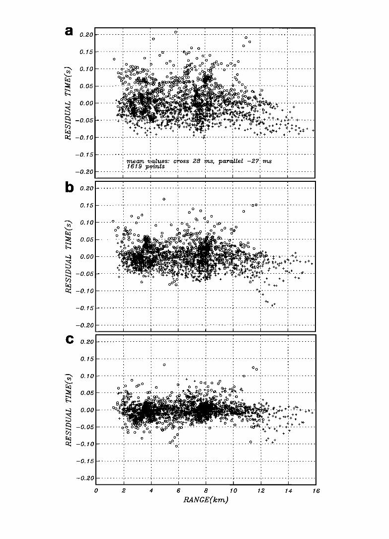
Figure 8a shows the range dependence of the residuals from ray paths along ridge-parallel (pluses) and ridge-crossing (circles) azimuths after correcting only for the average one-dimensional average velocity stmcture. If anisotropy were present at all depths, the difference in the residuals along the two sets of azimuths would increase with range. We see instead a more or less constant residual for each azimuth, suggesting the anisotropy is associated with ranges of less than 2 km. The ray path turning point depths for ranges of 2 km are at about 500 m. These data con-


strain the azimuthal velocity anisotropy to be within the upper 500 m or less of the oceanic crust. Figure 8b shows the residual travel time after removing layer thickness variability as determined by an inversion that did not allow anisotropy. The RMS residual of Figure 8b is 33 ms, a 16-ms RMS reduction, or 58% variance reduction from Figure 8a. Figure 8c shows the residuals for an inversion that allows anisotropy as well as layer thickness variability. The RMS residual is then reduced to 24 ms, a 78% variance reduction from the residuals of Figure 8a. The remaining RMS residual is greater than that expected from the travel time measurement accuracy error and is probably the result of the fol- lowing causes, in order of importance: (1) lateral heterogeneity of the extrusive layer at scales too small to be mapped with this data set, (2) arrival time picking errors, and (3) lateral heterogeneity within the sheeted dikes.

The layer thickness residuals after the removal of the anisotropy determined by inversion are plotted in map form in Figure 9. Fast arrivals (thins) are plotted as circles and slow arrivals (thicks) are plotted as pluses, with the size of the symbol representing the magnitude of the residual. These travel time variations can be interpreted as thickness variations in the shallow low-velocity layer, as the residuals are plotted at the ray entry point for the shot.

Figure 10 is the layer thickness map from the inversion; time was converted to depth using the average velocity of 2.8 km/s and the average ray path angle from the vertical of 35ø: 10 ms is equivalent to 23 m. The map has been contoured with interpola- tion in the areas of no data.

The range of velocities which we consider probable for the extrusive layer rocks is insufficient to explain more than a small part of the observed travel time residuals as being due to lateral velocity variations within the extrusive layer. With layer velocity fixed at 2.8 km/s, 90% of the apparent layer thicknesses fall within the range from 200 m to 550 m. If we choose an extreme case where the average velocity of the extrusive layer was to vary laterally by 30% (2.4 to 3.2 km/s), this would be equivalent to an apparent thickness variation of 100 m. Lateral velocity variability is probably much less than 30%, and we consider it to be a small effect compared to extrusive layer thickness variability. To invoke lateral velocity changes of greater than this magnitude would be difficult because the lowest velocities recorded in

seafloor basalts are about 2.1 km/s [Kappus, 1991]. Velocities of as high as 4 km/s are seen within the extrusive zone of the Troo- dos ophiolite, associated with intrusive bodies [Eleftheriou and Schoenharting, 1987], but if such intrusive bodies were present on the JDFR, we would expect evidence of them from the seafloor mapping in this area.

To search for lateral variability of anisotropy, the inversion procedure was performed with various combinations of up to four different geographic regions. No significant difference in anisotropy was observed between the chosen regions. The peak-to- peak anisotropy value from the inversion over the complete data set is 61 +2 ms with a fast direction azimuth of 21 ø +5 ø. This is

equivalent to a velocity of 2.25 km/s in the slow direction and 3.35 km/s in the fast direction. The best fitting azimuth is comparable to the ridge alignment of 19 ø .

Discussion

Comparison With the Northern Juan de Fuca Ridge

Previous studies have modeled seismic refraction data from the

northern Juan de Fuca ridge [Cudrak, 1988; White and Clowes, 1990; Cudrak and Clowes, 1993] using two-dimensional methods.

These results are compatible with those shown in this paper (Fig- ure 4), although our geologic interpretation differs. These northern JDFR data show branch 1 refractions on all 15 lines examined, although sometimes only on a single trace. Their two- dimensional analyses result in an average low-velocity layer model where velocity increases from 2.56 km/s at the surface to 2.76 krn/s at the base of a 400-m-thick layer. The similar water depths and bathymetric variability allow comparison of results. All lines in the northern JDFR data set show distinct shallow

refractions, while only 21 of 34 lines from our southern JDFR data show such refractions. This is consistent with the slightly thinner low-velocity layer and slightly higher average velocity we observe at the southern JDFR site, both factors which tend to mask branch 1 refractions at our location.

Interpretation of Velocity-Depth Profiles

The upper 230 m of our velocity depth profiles are interpreted as the zone of extrusive basalt. The velocity transition from 230 m (2.9 km/s) down to 370 m (4.7 km/s) is interpreted as a mixed zone of dikes, sills, and extrusives. Velocities below 370 m are

comparable to those at other sites on zero-age fast or medium spreading rate crust and are interpreted as sheeted dikes (Figure 4). This interpretation differs from that of Cudrak and Clowes [1993] and Rohr et al. [1988], who interpret a similar velocity increase on the northern JDFR as a metamorphic front above the lithologic boundary at the top of the sheeted dikes. Arguments for a metamorphic front interpretation are based primarily on evidence from boreholes in older oceanic crust where the extrusive

rocks commonly have seismic velocities of 5 km/s [Moos et al., 1990] and from the observed thinning of the shallow low velocity layer with crustal age [Jacobson, 1992]. Harding et al. [1993] argue for placing the top of the sheeted dikes at the base of the velocity transition zone (about 5.0 km/s) from work on the East Pacific Rise (EPR). Their arguments include observations that while the low-velocity layer generally thickens with increasing distance from the axis out to several kilometers, this growth is not compensated by thinning of the underlying layers. Other support for interpreting our velocity gradient at 4.7 km/s as the top of the dikes is provided by Eleftheriou and Schoenharting [1987], who see a similar correlation in their seismic refraction data from the

Troodos ophiolite where drillholes provide control. The velocity transition in our data probably corresponds to a

zone of mixed extrusives and sills as seen at Hess Deep [Fran- cheteau et al., 1992] rather than a porosity change within the extrusive layer as seen in hole 504B [Wilkens et al., 1991]. The thickness of the low-velocity layer within about 1 km of the axis is considerably thinner [Christeson et al., 1992], presumably because this zone represents an immature stage in the formation of oceanic crust, such that the shallow low-velocity layer is not yet of full thickness. The Hess Deep observations report a mixed lithology transition zone between the dikes and the pillows with a thickness ranging from zero to 500 m. Comparison between the EPR velocity depth profiles and Hess Deep lithologic profiles sup- ports a correlation of velocities less than about 3 km/s with the extrusives and velocities between 3 km/s and 4.7 km/s with the

lithologic transition zone. Figure 4 shows velocity depth profiles of zero-age crust for five

separate areas to allow comparison. Two of these areas are on the fast spreading EPR, at 9ø33'N and 13ø13'N, where shallow velocity structure has been determined using expanding spread profiling [Harding et al., 1989; Vera et al., 1990] and mapped laterally using wide aperture profiling [Kappus, 1991] and multichannel reflection profiling [Harding et al., 1993]. The differ-

a

', , ' 0 0 ' , 0 , , , , ,

,' ............ D' ..... O•C• ....................... 0.15 .......... , o o'. o o ', o ', o " o o o ', ',

:o• ,• o o: _•.,.*ooø: •%OoO:o ø : : O. 10 ........ o- :d•o•' o•b .............. •*• o .... c• .... o' -: ......... : ......... : ........

o_o: •,•;•O•o ..ø _: i}•_ '•il• ' ø ' ' •o'"o _• .... oo oo ,• o : %o : : ..... : ......... : ........ 0.05 ........... _;., •- - -.•-c• , •.a.- - •o'-"-;.,' ,• ',.-• , O-o •q:•"o ' "-' • •,.•o_•o•o Oo o • :o :

o. o o ...... '/--• :•,.•t•: ¾--: ........ ....... . .':+7-++- .-W•+.•I•.•_• .•2...•$•.'.+..••!•'. ,,,*,•,• ¾•, • +; • + + +. +:. +

-0.10 ......... : .... "---+- '--* ....... : ..... -+---+•: .................. : ........ +- -- -+- ..... , ,

,

,

, ,

-0.15 ............................ ' ' - ........ mean values: c',ross 28 ,ms, para, llel -27: ms ,

1619 pbints .... -0.20 - ' .... -

0.2,0

', ', o ', ', ', ', ',

O. 15 ........ " ......... : ......... : ......... '" ......... " ...... oe-: ......... : ......... ', ', : o ø o', ', o ', ',

/ : o oø : : ..; o : :

o. • o L .... o.._: .... o .... :-• .... b' ':' o-•_- --•- . "-,,o- ¾c• .... : ......... : ......... : ........ 0 ,0 , 0 0 + , 0 0 ,0 , , 0 , 0 , , 0 , 0 0 0 , , • •o• -, o •o••,•o o , ,

• 0 v , 0 •0 , , , o. o5 ........ • • - -•• •- - • •- -+-•-••- - -o ............................. + •.. o '•• •_•W o, o •_••• •9•_ ao• ' '

o. oo ....... •••. ' ••••?••+•-,- ß .... +-• .....

- O. 0 5 .......... -• ' •• • $*•+•+••• '• + ' *" '•' i- •*' ' '• r .................. + •*,.'+ • • "• W•..• • + ' .:+• +.•+-• + + + + o : oq, : o :+ + , o o, , , + •

-0.10 ................... ' ............................ ' ....... **: ................. : +

++ ++

-0.20 I I I I I

, , , , ,

0.20 ............................................................................... , , ,

, , , , , ,

, , , , , , ,

, , , ,

, , , , ,

0.15 .................................................. . , , , , , ,

' ' o , ,

, ,, , o 0 , . , ,

, , , , .

O. 10 ........................................... o ........................ : o : : + + o• o o : : :

o :o •o : o • o o :o o• ,2o • ', o. o5 ....... ,.•-• ..... • ...... •- -k *o•-ea-• •o- •*•-? • ...... i ......... • .........

0 •. • • + • ß +++ O. O0 ...... o+l .• :•, .... +. •,... + +• .' ++

• ' + +

-o. o5 ........ o• • , ' ....... :'• ....... : ..... •*'•:'+'< •*k ......... '80 oo, o• , , , ', o , , . ++ + , -0.10 ........ ' '•e" ......... ' .......... + ' o] , '

,

,

, ,

-0.15 ' ' , ,

,

, ,

,

-0.•0 i I I I I I

0 2 4 6 8 10 12 14 16

•••(•)

45 ø 05'N

o.

+++

44 ø 55'N

o

44 ø 50'N

+.

,+ + +

++

_½ +

o+ o+

4-

2oO O O

o

ß o ,

o

o o o o

ß ø o(• ,¸

130ø20'W 130 ø 15'W 130 ø 10• r

••' +=SOres 07' 128m

Figure 9. Map of travel time residuals after removal of anisotropy term, such that the residual is proportional to the relative layer thickness plus errors. Pluses are slow arrivals, circles are fast arrivals, and the size of the symbols represents the magnitude of the residual.

Figure 8. The travel time residuals for rays within 22.5 ø of the cross axis direction, shown as pluses, and within 22.5 ø of the axis parallel direction, shown as circles, are plotted versus range. Since increasing anisotropy is not observed with range, no anisotropy for portions of the ray path deeper than 500 m (corresponding to 2 km range) is required. (b) The travel time residuals plotted as in Figure 8a after removal of layer thickness but not allowing for anisotropy in the inversion resulting in a 58% variance reduction. (c) The travel time residuals plotted as in Figure 8a after removal of layer thickness variation and after applying an anisotropy term resulting in a 78% variance reduction.


45 ø 05'N

45 ø 00'N

44 ø 55'N

44 ø

50'N

:.

130ø20%V 130 ø 153N 130 ø 103N

Figure 10. Thickness in meters of the low-velocity layer, as inferred from travel time residuals (the velocity is assumed to be 2.8 krn/s and ray paths to be 35 ø from the vertical). We interpret the low-velocity layer as extrusives.

ence in low-velocity layer thickness across segment boundaries, such as between 9ø33'N and 13ø13'N, provides a possible explanation for the 150 m to 250 rn variation in the thickness of the pil- low basalts observed in EPR crust at the Hess Deep [Francheteau et al., 1992], between measured sections 20 km distant from one

another. These sections may be in different segments depending on the history of propagators in the area.

On the medium spreading rate JDFR at 48øN [Cudrak, 1988; Cudrak and Clowes, 1993] and at 45øN (this paper) the average thicknesses of the low-velocity layer are 400 and 350 m, respectively. However, a variability of + 150 m or more is observed on wavelengths of a few kilometers. Such rapid lateral variability in low-velocity layer thickness has not yet been observed on the EPR except within a kilometer of the axis where the extrusive layer is being formed [Christeson et al., 1992]. This difference highlights the need for different models of crustal formation at the EPR and

JDFR which might relate differences in spreading rate, magma supply, and episodicity. The velocity profile from the Mid- Atlantic Ridge (MAR) [Purdy and Detrick, 1986] is considerably slower than the others, making it less directly comparable. How- ever, assuming the shallowest steep velocity increase corresponds to the extrusive basalt to dike transition, the thickness of the

extrusive basalt layer is significantly thicker than seen elsewhere. The existing data suggest that at fast spreading ridges the extrusive volcanic layer is thinnest and laterally relatively homo- geneous, at least within a ridge segment. On medium rate ridges the thickness is intermediate with considerable short-wavelength variability, and on slow spread ridges the low-velocity layer is thickest with unknown variability.

Azimuthal Anisotropy

Ridge-parallel fracturing, as seen from submersibles [Kappel and Normark, 1987], would produce azimuthal anisotropy with the fast direction parallel to the ridge axis. The range versus residual plot of Figure 8a demonstrates that seismic anisotropy occurs entirely in rocks at depths of 500 m or less. Given the 350-m average thickness of the low-velocity extrusive layer, it is probable that the anisotropy is associated with this lithologic unit. In estimating the velocities associated with the anisotropy, we suggest a probable case using the measured travel time difference of 61 ms and assuming a 350-m-thick anisotropic layer with horizontal velocities of 2.25 and 3.35 km/s. In this case, the refracted ray paths have an angle from vertical within the anisotropic layer of 29 ø and 38 ø in the slow and fast directions, respectively. We might expect the degree of anisotropy within the shallow low- velocity layer to vary laterally because the processes forming and healing fractures are active within the experiment area. No such variation was detected that was statistically significant, although resolution is limited to at best an area about 1/4 of that of the total

data set in order to have a statistically stable inversion that included rays to several OBSs over a broad range of azimuths. It is possible to interpret the post inversion residuals as lateral changes in anisotropy but difficult to judge the accuracy of such interpretation. The observed differences between shot lines on some of the cross sections in Figure 11 could be caused by such anisotropy variability.

To understand the relationship between anisotropy and the character of the rock, we also need information on porosity, crack density, crack aspect ratio, and crack vertical dip [Wilkens et al., 1991]. The average porosity within the upper several hundred meters of crust within the experiment area has been determined to be about 17% using seafloor gravity measurements [Stevenson et al., this issue]. We have no independent measurements of the crack density, aspect ratio, or dip. Improved theory or empirical relationships or other geophysical measurements are needed to determine these parameters in order to better interpret our measurements of anisotropy.

Seismic refraction experiments have measured compressional wave azimuthal anisotropy of up to 29% [(Vmax-Vmin)/Vmax] in fractured limestones [Bamford and Nunn, 1979] and up to 42% in fractured igneous rocks [Park and Simmons, 1982]. Fractures at mid-ocean ridges are likely to be more consistently aligned than those seen in these continental rocks, where several different fracture orientations are commonly present in the same rock. Consid- ering these continental examples, it is not surprising to find 33% anisotropy in our JDFR experiment. Current theoretical models [Crampin, 1991; Berge et al., 1992] do not explain such large degrees of anisotropy, and empirical relationships have not yet been developed to utilize the anisotropy observations in interpreting porosity type.

Other experiments observing shallow crustal azimuthal anisotropy in near zero age crust [Caress et al., 1992; Cudrak, 1988] and crust more than a million years old [Shearer and Orcutt, 1986; Stephen, 1985], have found a ridge-parallel fast direction, with the exception of White and Whitmarsh [1984] which is on


.2400 2800

3200

2400

2800

3200

2400 2800

3200

_2400 -

2800-

3200 0

N I I½ N I I½'

x n x-N1

•-N6 o-N8

N6 W"

x x-N1

/' -N6 O-N8

I

_

øo • • • •%• •• ..... .•( .---•.•t

• • x,' o-s6 /•-S7

5 10 15 20 25 30

Figure 11. Four sections perpendicular to the ridge showing bathymetry below the air gun lines. Also shown are the time residuals from each shot to each of several OBSs interpreted as a thickness variation of the shallow low- velocity layer. The most obvious patterns seen in the residual travel time map and in the cross sections are a generally thicker extrusive layer west of the axial valley and a thin extrusive layer within the axial valley at 45ø58'N.

Atlantic crust of more than a million years age. Caress et al. [1992] observed about 100-ms peak-to-peak azimuthal variation in residual trayel times from the EPR axis at 12ø50'N, with no apparent range dependence. That result is similar to the 110-ms variation we see on axis (Figure 5b). Unfortunately, the data of Caress et al. lacks a sufficient number of short range ray paths to be able to restrict the depth interval over which the anisotropy occurs and part of the perceived anisotropy is probably associated with ridge structure. It is probable that a similar fracture-induced anisotropy exists at both sites. It may be that such anisotropy is common on fast and medium spreading rate ridges, as few of the seismic data sets from ridges are suitable for this type of analysis.

Extrusive Layer Thickness Variability

Figures 9, 10, and 11 show travel time residuals as variations in the shallow low-velocity or extrusive layer thickness. The cause of much of the thickness variability is presumed to be the episodic nature of intermediate rate spreading ridges [Kappel and Ryan, 1986] where during periods of decreased magmatism extension continues, resulting in tilted fault blocks on a scale of 1 or 2 km across. The direction of rotation on these fault blocks is seen in

the cross section of Figure 11, where apparent fault offsets on a scale length too short to be seen in the smoothed thickness map are evidenced on the west flank of the ridge. The low side of these


fault blocks are likely filled with talus and extrasives [Alexander and Harper, 1992] resulting in lower-velocity rock extending to a greater depth. Similar faults have been mapped seismically in the Troodos Ophiolite [Eleftheriou and Schoenharting, 1987]. This process would be expected to account for the observed greater variability in thickness on lines across the strike of the faults than parallel to them.

The extrusive layer is generally thicker west of the Cleft segment axial valley. One possible explanation for this asymmetry in extrusive layer thickness may be that the seafloor slope within the axial valley maintains a westward tilt (as currently exists), causing erupted pillows and flows to preferentially flow westward becoming part of the Pacific plate. Such a hypothesis is supported by the western axial valley escarpment being higher on the northern Cleft segment, suggesting a more active listric fault on this side. The mapping of a recent flow [Embley et al., 1991] on the north- em Cleft segment shows the flow to be entirely west of the cleft or fissure, the site of hydrothermal venting which is presumed to be the plate boundary.

The thinnest extrusive layer, about 200 m, is seen within the axial valley at the northern end of the Cleft segment. This is an area where hydrothermal activity has considerable surface expres- sion and is the site of a recent sheet flow. As shown by Christe- son et al. [ 1991 ] on the EPR, the low-velocity layer can be as thin as 60 m directly on the ridge axis of the EPR, corresponding to the presumed center of the zone in which the extrusive layer is being formed. The axial regions with the thinnest low-velocity layer are interpreted as areas in which new oceanic crust is most actively being spread and is still immature. The areas of thin extrusives off axis are interpreted as regions in which the crust was rapidly rifted, shifted, or faulted out of the zone of active volcanism.

The extrusive layer thickness is most variable in the vicinity of the Cleft-Vance overlapping rift zone. This might be expected considering the transform faulting, spreading center offset, and constructive volcanism associated with the overlapping rift zone. This overlapper appears relatively quiescent at present, however, two tectonic earthquakes, similar to those recorded by Cooper et al. [1987] at the Galapagos propagating rift, were detected near OBS N2 during the 12 days of continuous OBS recording. One of these has a hypocenter depth of 1.8 km.

A comparison between the Bouguer seafloor gravity map of Stevenson et al. [this issue] and the extmsive layer thickness map of Figure 10 shows the thick extrusive layer at the southern end of the Vance segment corresponds with a gravity minimum. This is as expected as the thick extrusive layer with its low density will yield a Bouguer gravity low.

Conclusions

The Cleft and Vance segments of the JDFR have an average velocity structure with a shallow low-velocity layer of 350 m in thickness. It is interpreted to correspond to the thickness of the extrusive volcanic layer. An average velocity of 2.8 km/s +0.16 km/s was estimated for the low-velocity layer as determined by direct refraction paths entirely within the shallow layer. Seismic compressional velocity anisotropy is observed. It is confined to the upper 500 m or less of the oceanic crest. The ridge-parallel horizontal velocity is about 3.35 km/s and the ridge perpendicular velocity is about 2.25 km/s. The anisotropy is presumed to be caused by open fractures preferentially aligned with the ridge axis. Extrusive layer thickness varies from 200 to 550 m and is presumably related to the volcanic processes by which the layer is formed, so that the variability on the JDFR at this site is much greater than that observed on the EPR.

Acknowledgments. This research received support from the NOAA Vents Program. We thank LeRoy Dorman, Bob Embley, Alistair Harding, Anne Trehu, and Doug Toomey for helpful suggestions. We thank Gerard Fryer and anonymous reviewers for their reviews. We thank Peter Shaw for the use of his

interactive travel time modeling software, Perry Crampton for the air gun operations, Paul Henkart for his assistance with the SIOSEIS seismic processing software, Vince Pavlicek, Phil Hammer, Wayne Crawford, and Duncan McGehee for assistance at sea, and the officers and crew of the NOAA ship Discoverer who provided excellent sea-going support.

References

Aki, K. A., and P. G. Richards, Quantitative Seismology Theory and Methods, pp. 695-697, W. H. Freeman, New York, 1980.

Alexander, R. J., and G. D. Harper ,The Josephine Ophiolite: An Ancient Analogue for Slow-to-Intermediate-Spreading Oceanic Ridges, In: Ophiolites and their Modern Oceanic Analogues, pp. 3-38, Geological Society Special Publication No. 60, edited by L. M. Parson, B. J. Murton and P. Browning, Geological Society, London, 1992.

Baker, E. T., G. J. Massoth, and R. A. Feely, Cataclysmic venting on the Juan de Fuca Ridge, Nature, 329, 149-151, 1987.

Berge, P. A. G. J. Fryer and R. H. Wilkens, Velocity-Porosity Relationships in the Upper Oceanic Crust: Theoretical Considerations, J. Geophys. Res., 97(Bll), 15,239-15,254, 1992.

Bamford, D., and K. R. Nunn, In situ seismic measurements of

crack anisotropy in the Carboniferous limestone in northwest England, Geophys. Prospect., 27, 322-338, 1979.

Caress, D. W., M. S. Burnett and J. A. Orcutt, Tomographic image of the axial low-velocity zone at 12ø50'N on the East Pacific Rise, J. Geophys. Res., 97, 9243-9263, 1992.

Chadwick, W. W., R. W. Embley, and C. G. Fox, Evidence for volcanic eruption on the southern Juan de Fuca Ridge between 1981 and 1987, Nature, 350, 416-418, 1991.

Christeson, G. L., G. M. Purdy, and G. J. Fryer, Structure of young crest at the East Pacific Rise near 9ø30'N, Geophys. Res. Lett., 19, 1045-1048, 1992.

Cooper, P. A., P. D. Milholland, and F. K. Duennebier, Seismicity of the Galapagos 95.5øW propagating rift, J. Geophys. Res., 92, 14,091-14,112, 1987.

Cox, C. S., T. Deaton, and S.C. Webb, A deep sea differential pressure gauge, J. Atmos. Oceanic Technol., 1, 237-246, 1984.

Crampin, S., Wave propagation through fluid-filled inclusions of various shapes: interpretation of extensive-dilatancy anisotropy, Geophys. J. Int., 104, 611-623, 1991.

Crampin, S., and D. Bamford, Inversion of P-wave velocity anisotropy, Geophys. J. R. astr. Soc.,, 49, 123-132, 1977.

Cudrak, C. F., Shallow crustal structure of the Endeavour Ridge segment, Juan de Fuca Ridge, from a detailed seismic refraction survey, thesis, 162 pp., Univ. of B.C., Vancouver, 1988.

Cudrak, C. F., and R. M. Clowes, Crustal structure of Endeavour Ridge segment, Juan de Fuca Ridge, from a detailed seismic refraction survey, J. Geophys. Res., 98, 6329-6349, 1993.

Detrick, R. S., A. J. Harding, G. M. Kent, J. A. Orcutt, J. C. Mutter, and P. Buhl, Seismic structure of the southern East Pacific Rise, Science, 259, 499-503, 1993.

Eleftheriou, S., and G. Schoenharting, A seismic velocity survey at the Agrokopia Mine, Cyprus: The velocity structure of a hydrothermally altered extrusive section of the Troodos


Ophiolite, In: Cyprus Crustal Study Project: Initial Report, Holes CY-2 and 2a, Geol. Surv. of Can., Paper 85-29, edited by P. T. Robinson, I. L. Gibson and A. Panayiotou, Geol. Surv. of Can., Ottawa, Ont., pp. 317-326, 1987.

Embley, R. W., W. Chadwick, M. R. Perfit, and E. T. Baker, Geology of the northern Cleft segment, Juan de Fuca: Recent lava flows, sea-floor spreading, and the formation of megaplumes, Geology, 19, 771-775, 1991.

Fox, C. G., W. W. Chadwick, and R. W. Embley, Detection of changes in ridge-crest morphology using repeated multibeam sonar surveys, J. Geophys. Res., 97, 11,149-11,162, 1992.

Francheteau, J. R. Armijo, J. L. Cheminee, R. Hekinian, P. Lonsdale, and N. Blum, Dyke complex of the East Pacific Rise exposed in the walls of Hess Deep and the structure of the upper oceanic crust, Earth and Planet. Sci. Lett., 111, 109-121, 1992.

Harding, A. J., J. A. Orcutt, M. E. Kappus, E. E. Vera, J. C. Mutter, P. Buhl, R. S. Detrick, and T. M. Brocher, The structure of young oceanic crust at 13øN on the East Pacific Rise from expanding spread profiles, J. Geophys. Res., 94, 12,163-12,196, 1989.

Harding, A. J., G. M. Kent, and J. A. Orcutt, A multichannel seismic investigation of upper crustal structure at 9øN on the East Pacific Rise: Implications for crustal accretion, J. Geophys. Res., 98, 13,925-13,944, 1993.

Jacobson, R. T., Impact of crustal evolution on changes of the seismic properties of the uppermost ocean crust, Rev. Geophys., 30, 23-42, 1992.

Kappel, E. S., and W. R. Normark, Morphometric variability within the Axial Zone of the southern Juan de Fuca Ridge: Interpretation from SeaMARC II, SeaMARC I, and deep-sea photography, J. Geophys. Res., 92, 11,291-11,302, 1987.

Kappel, E. S., and W. B. F. Ryan, Volcanic episodicity and a non-steady state rift valley along northeast Pacific spreading centers: evidence from SeaMARC I, J. Geophys. Res., 91, 925- 940, 1986.

Kappus, M. E., A baseline for upper crustal velocity variations along the East Pacific Rise, thesis, 158 pp., Univ. of Calif., San Diego, 1991.

Karson, J. A., Seafloor spreading on the Mid-Atlantic Ridge: Implications for the structure of ophiolites and oceanic lithosphere produced in slow-spreading environments In: Proceedings of the Symposium "TROODOS 1987" edited by J. Malpas, E.M. Moores, A. Panayiotou, and C. Xanophontos, Cyprus Geol. Surv. Dept., Nicosia, 547-555, 1991.

Liebelt, P. B., An Introduction to Optimal Estimation, Addison- Wesley, Reading, Mass., 1967.

Lonsdale, P., Structural geomorphology of a fast-spreading rise crest: The East Pacific Rise near 3ø25'S, Mar. Geophys. Res., 3, 251-293, 1977.

Moos, D., P. Pezard, and M. Lovell, Elastic wave velocities within oceanic layer 2 from sonic full waveform logs in Deep Sea Drilling Project holes 395A, 418A, and 504B, J. Geophys. Res., 95, 9189-9207, 1990.

Morris, G. B., R. W. Raitt, and G. G. Shor, Jr., Velocity anisotropy and delay-time maps of the mantle near Hawaii, J. Geophys. Res., 74, 4300-4316, 1969.

Morton, J. L., N.H. Sleep, W. R. Normark, and D. H. Tompkins, Structure of the southern Juan de Fuca Ridge from seismic reflection records, J. Geophys. Res., 92, 11,315-11,326, 1987.

Murphy, K. M., and R. W. Embley, A morphologic and structural study of the Vance Seamount Chain: Relationship to volcanism on the Juan de Fuca Ridge, Eos, Trans. AGU, 69, 1503, 1988.

Nicolas, A., Structural Studies of Ophiolites and Dynamics of Ocean Lithosphere, Kluwer Academic, Boston, Mass., 1989.

Park, S., and G. Simmons, Crack-induced velocity anisotropy in the White Mountains, New Hampshire, J. Geophys. Res., 87, 2977-2983, 1982.

Purdy, G. M., and R. S. Detrick, Crustal structure of the Mid- Atlantic Ridge at 23 ø N from seismic refraction studies, J. Geophys. Res., 91, 3739-3762, 1986.

Purdy, G. M., L. S. L. Kong, G. L. Christeson, and S.C. Solomon, Relationship between spreading rate and the seismic structure of mid-ocean ridges, Nature, 355, 815-817, 1992.

Raitt, R. W., G. G. Shor, Jr., T. J. G. Francis, and G. B. Morris,

Anisotropy of the Pacific upper mantle, J. Geophys. Res., 74, 3095-3109, 1969.

Rohr, K. M. M., B. Milkereit, and C. J. Yorath, Asymmetric deep crustal structure across the Juan de Fuca Ridge, Geology, 16, 533-537, 1988.

Shearer, P.M., and J. A. Orcutt, Compressional and shear wave anisotropy in the oceanic lithosphere: The Ngendei seismic refraction experiment, Geophys. J. R. Astron. Soc., 87, 967- 1003, 1986.

Stephen, R. A., Seismic anisotropy in the upper oceanic crust, J. Geophys. Res., 90, 11,383-11,396, 1985.

Stevenson, J. M., J. A. Hildebrand, M. A. Zumberge, and C. G. Fox, An ocean bottom gravity study of the southern Juan de Fuca Ridge, J. Geophys. Res., this issue.

U.S. Geological Survey (USGS) Juan de Fuca Study Group, Submarine fissure eruptions and hydrothermal vents on the southern Juan de Fuca Ridge: Preliminary observations from submersible Alvin, Geology, 14, 823-827, 1986.

V era, E. E., J. C. Mutter, P. Buhl, J. A. Orcutt, A. J. Harding, M. E. Kappus, R. S. Detrick, and T. M. Brocher, The structure of 0- to 0.2-m.y.-old oceanic crust at 9øN on the East Pacific Rise from expanded spread profiles, J. Geophys. Res., 95, 15,529- 15,556, 1990.

White, D. J., and R. M. Clowes, Shallow crustal structure beneath

the Juan de Fuca Ridge from 2-D seismic refraction tomography, Geophys. J. Int., 100, 349-367, 1990.

White, R. S., and R. B. Whitmarsh, An investigation of seismic anisotropy due to cracks in the upper oceanic crust at 45øN, Mid-Atlantic Ridge, Geophys. J. R. Astron. Soc., 79,439-467, 1984.

Wilkens, R. H., G. J. Fryer, and J. Karsten, Evolution of porosity and seismic structure of upper oceanic crust, J. Geophys. Res., 96, 17,981-17,996, 1991.

B.D. Comuelle, J. A. Hildebrand, M. A. McDonald, and S.C.

Webb, Scripps Institution of Oceanography, University of California, San Diego, La Jolla, CA 92093-0205. (e-mail: [email protected])

C. G. Fox, National Atmospheric and Oceanic Administration, Pacific Marine Environmental Laboratory, Hatfield Marine Science Center, Newport, OR 97365.

(Received November 3, 1992; revised August 16, 1993; accepted October 5, 1993.)

Seismic structure and anisotropy of the Juan de Fuca Ridge at 45°N

Documents

Transcript of Seismic structure and anisotropy of the Juan de Fuca Ridge at 45°N