mathematics

Article

Sectorial Fuzzy Controller Plus Feedforward for the TrajectoryTracking of Robotic Arms in Joint Space

Andres Pizarro-Lerma 1 , Victor Santibañez 2 , Ramon Garcia-Hernandez 2,* and Jorge Villalobos-Chin 2

Citation: Pizarro-Lerma, A.;

Santibanez, V.; Garcia-Hernandez, R.;

Villalobos-Chin, J. Sectorial Fuzzy

Controller Plus Feedforward for the

Trajectory Tracking of Robotic Arms

in Joint Space. Mathematics 2021, 9,

616. https://doi.org/10.3390/

math9060616

Academic Editor: Mihaela Colhon

Received: 7 February 2021

Accepted: 11 March 2021

Published: 15 March 2021

Publisher’s Note: MDPI stays neutral

with regard to jurisdictional claims in

published maps and institutional affil-

iations.

Copyright: © 2021 by the authors.

Licensee MDPI, Basel, Switzerland.

This article is an open access article

distributed under the terms and

conditions of the Creative Commons

Attribution (CC BY) license (https://

creativecommons.org/licenses/by/

4.0/).

1 Instituto Tecnologico de Sonora, 5 de Febrero 818 sur, Ciudad Obregón C.P. 85000, Sonora, Mexico;andres.pizarro@itson.edu.mx

2 Tecnologico Nacional de Mexico/Instituto Tecnologico de La Laguna, Blvd. Revolucion y Av. InstitutoTecnologico de La Laguna S/N, Torreon C.P. 27000, Coahuila, Mexico; vsantiba@itlalaguna.edu.mx (V.S.);jorgevchin@gmail.com (J.V.-C.)

* Correspondence: rgarciah@correo.itlalaguna.edu.mx; Tel.: +52-871-705-1324

Abstract: In this paper, we propose a Sectorial Fuzzy Controller (SFC) with a feedforward compensa-tion of the robot dynamics in joint space, evaluated at the desired angular positions, velocities, andaccelerations, applied to the trajectory tracking of all revolute joints robotic arms. Global uniformasymptotic stability proof applying the direct Lyapunov theorem, is introduced for this new controlscheme by using a strict Lyapunov function. This strict Lyapunov function is the first one withinthe field of fuzzy control that is applied to the trajectory control of robotic manipulators. With thisstrict Lyapunov function, a sensitivity analysis was also computed for this novel control scheme.Additionally, physical and simulation experimental results are given in comparison to the originalcontrol scheme, in which this new controller is inspired: the Proportional-Derivative (PD) controllerplus feedforward compensation. The experimental results yielded better performance for the newfuzzy control scheme when compared to the classical structure, in both the joint position errors forsimilar or smaller values of applied torques, showing the expected tolerance to parametric deviationsand uncertainties that all fuzzy controllers possess.

Keywords: sectorial fuzzy controller; robotic arm; tracking control; feedforward compensation; strictlyapunov function

1. Introduction1.1. Motivation

Most industrial robotic arms are controlled in trajectory tracking tasks by applying aProportional + Integral + Derivative (PID) controller, although it has not been proven thatthis type of controller can actually approach to a zero steady-state error for that specifictype of tasks. From the original control schemes that were applied to robotic arms, onlythe computed-torque and the Proportional-Derivative (PD) plus feedforward schemeshave been proved to tend asymptotically to zero steady-state error for trajectory trackingin robotic arms, whose proof extends to a global asymptotic stability. The latter impliesthat the initial position error can be of any value and both of the aforementioned controlschemes will achieve that the robotic arm follows the desired trajectory. Both of the controlschemes use a PD controller plus the whole robot dynamics connected in some fashion;in the case of the Computed-Torque Controller (CTC), it manages to eliminate all of thenon-linearities of the robot model and turn the closed-loop equivalent into a linear system.In the case of the PD plus feedforward (PD + ff), the feedforward block is composed bythe robot model evaluated at the desired angular positions, velocities, and accelerations,which yields an excellent tracking performance, comparable with that of the CTC [1].Nonetheless, a robot is highly nonlinear, with variations in its parameters at almost eachpoint of execution. Within the various existing control approaches to the motion control ofrobots, fuzzy controllers can be a robust and efficient alternative in cases where it is difficult

Mathematics 2021, 9, 616. https://doi.org/10.3390/math9060616 https://www.mdpi.com/journal/mathematics

Mathematics 2021, 9, 616 2 of 40

to have an exact model of the plant to be controlled, or there are many disturbances andchanges in some of its key parameters. Additionally, fuzzy control allows for combiningheuristic elements with the analytical models. Once some guidelines to design fuzzycontrollers with sectorial properties, named Sectorial Fuzzy Controllers (SFCs), whichenable their stability analysis, were given in [2], a few works on the motion control ofrobot manipulators emerged: in [3], a computed torque control with a SFC instead of a PDcontroller, showed excellent results in physical experiments in the tracking motion controlof a 2 degree of freedom (2-DOF) robotic arm. A SFC with gravity compensation wasapplied to a 2-DOF robotic manipulator in order to regulate its joint positions in [4], againshowing excellent results in its physical experiments, and adding the property of havingbounded torques. In [5], a saturated fuzzy control for regulation of robot manipulators withactuator constraints was presented. This controller is formed by joining a saturated integralaction with the SFC, thus forming some sort of sectorial fuzzy PID. A global asymptoticstability proof using Lyapunov’s direct method was outlined with all of the assumptionsmade by the authors never proven. In that paper, they only presented the simulation resultsin Matlab, and without considering the frictions in the robot model.

All of these control approaches use a Mamdani type SFC as its core element; neverthe-less, there exists the Takagi–Sugeno (T-S) counterpart of fuzzy controllers that has beenapplied to the control of mechanical or mechatronics systems: in [6], a T-S descriptor wasemployed to control a 2-DOF robotic manipulator with elastic joints and dry friction. Thetracking control design and stability assurance is reformulated as optimization problembased in the solution of a Linear Matrix Inequality (LMI). All of the experiments wereperformed in simulations in Matlab. Two fuzzy nonlinear methodologies to perform tra-jectory tracking of a Furuta pendulum were compared in [7] while using an exact convexrepresentation, and a dynamic output regulation, which does not solve the nonlinear partialdifferential equations better known as the Francis–Isidori–Byrnes (FIB) equations. In theend, the fuzzy approach T-S yielded better results than the dynamic output regulation ap-proach. The work reports physical experimental results. In [8], a 3-DOF robot is controlledin simulations via enH∞ approach. The presented results are excellent after designing 16matrices for the T-S fuzzification process. However, as with all T-S control approaches, themechanical model has to pass through an extensive algebraic manipulation to format itsequations to be used in the LMI formulation, and, by doing so, the obtained results canonly be applied to the specific plant, for which the fuzzy T-S control was designed.

Adaptive and recursive neural networks have also been applied to the task of motiontracking in robots, as in [9], where a robust adaptive Recurrent Fuzzy Wavelet FunctionalLink Neural Network (RFWFLNNs) that was based on dead zone compensator for Indus-trial Robot Manipulators was presented. The paper presents an extensive stability analysis,using Lyapunov, Lasalle invariance theorem, and Barbalats Lemma. However, none ofthose theorems can be applied for the stability analysis of their approach, since its controllaw possesses a discontinuity at the origin. The simulation and physical experimentson a 3-DOF robotic arm are presented, showing excellent results. The problem is thatthere are over ten matrices that must be computed at every sample period to be able tokeep those excellent results. In [10], an adaptive neural network is used as a feedforwardcompensator for a nonlinear saturated PD controller. Again, the number of elements tobe computed at every sample time is very large. This work presents both simulation andphysical experiments.

Although sliding-mode control is ill advised in any application that involves a me-chanical system, due to the destructive nature of the chattering phenomena that is the heartof this type of control approach, high strides have been made to cope with the chatteringproblem, and using fuzzy logic: a fuzzy-based sliding mode controller that was appliedto single-input single-output nonlinear systems was developed in [11] and applied to theregulation control of a one-link pendulum. Extensive Lyapunov analysis is presented inthis work. A Mamdani fuzzy system is applied to reduce the chattering and excellent

Mathematics 2021, 9, 616 3 of 40

results are presented for the control of the pendulum, since no mathematical model isconsidered for the design of the controller with good results.

From all of the previous references, we can conclude that either the work presentedis only applicable to the plant for which they are making the design of the controller,as in [6–8], or the controller requires such extensive computing [9] that makes it prohibitiveits application in typical industrial robot manipulators, or it could be applied to robots iftheir work can be extended to more than one link [11]. Additionally, in only half of thepapers, a full stability analysis was presented, and none of the previous works have founda strict Lyapunov function for the stability analysis of its control approach.

In previous works, where the SFC was applied to ensure position global regulation [4]and global motion trajectory tracking [3] for robot manipulators, present as a commonfeature that the respective closed-loop systems are autonomous. However, the motiontrajectory tracking problem for robot manipulators with feedback or feedforward compen-sation usually leads to nonautonomous nonlinear closed-loop systems. The main obstaclefor ensuring global uniform asymptotic stability (GUAS), in this class of systems, is thelack of a strict Lyapunov function (a decrescent and radially unbounded, globally positivedefinite function, whose time derivative is a globally negative definite function). Withthe goal of overcoming such a challenge, this paper introduces two new properties of theSFC developed in the lemmas included in Section 3.2, which allow us to construct a strictLyapunov function that leads to prove the GUAS of the robot manipulators in a closed-loopwith the SFC plus feedforward compensation. This strict Lyapunov function allowed forus to evaluate the sensitivity to changes in the elements of the robot model. In the presentpaper, we introduce, for first time, the application of the SFCs into nonautonomous closed-loop systems in robotic manipulators. Furthermore, the proposed control law has theuseful feature of providing bounded torques in accordance with the limits of the actuators.

1.2. Novelties

Our proposed control scheme possesses the following advantages with respect toother controllers reviewed:

• A strict Lyapunov function that guarantees full global uniform asymptotic stability,which, in turn, guarantees that the robot manipulator applied in this controller will beable to track the desired position trajectory, regardless of its initial angular position.

• The availability of a strict Lyapunov function allows for the sensitivity analysis to becarried out in a very direct way.

• Furthermore, the proposed control law has the useful feature of providing boundedtorques in accordance with the limits of the actuators. This is due to the outputboundedness characteristics of the SFC, and that its feedforward compensation isformed by the parameters of the robot, which are also bounded, as long as the desiredtrajectories are bounded.

• Besides, it is very simple to design, since almost all of the tuning parameters arealready defined by the sectorial guidelines that it has to adhere to, and the fact thatthe feedforward compensation block is fixed, with no parameters to change.

• Furthermore, due to its control law, the design of every SFC for every joint, for thiscontrol scheme, can be done individually, which is the contrary to the computed-torque sectorial controller, as defined in [3], where the SFCs of all the joints of a robothave to be tuned together, which, for an industrial robot of 3, 5 6, or 7 degrees offreedom, this becomes a very complicated task.

• Additionally, this independence among parts of the controller can be used to modelthe robot as a distributed or decentralized system which can lead to better and simplercontrol schemes.

• This controller is very simple to implement. There is no need for a high-end computerto run the code that implements this control scheme, which can be exported to an em-bedded system, like a low-cost Digital Signal Processor (DSP) or a Field Programmable

Mathematics 2021, 9, 616 4 of 40

Gate Array (FPGA), which, in turn, can reduce the costs for mass production of robotswhile using this type of controller.

• This control structure can be applied to any serial robot that is composed by n−linkswithout the need to change anything in its control law and design procedure, whilekeeping all of its properties.

• The application of this controller in industrial applications is limited to those, likewelding or painting, where there are not many changes in the mass parameters of therobot. The available applications can be extended to pick-and-place tasks or similar,if this controller is coupled with and adaptive block or estimator that can modify itsfeedforward compensation block.

Finally, the remainder of this paper is organized, as follows: first, a preliminariessection, where all the details related to the dynamics of robot manipulators with rigidlinks, the PD Control with feedforward compensation, and fuzzy logic controllers, arereviewed. Second, a complete section devoted to the SFC plus feedforward Compensation,the SFC definition with its original properties, and the properties that were proven for itsstability analysis. The stability analysis of the SFC plus feedforward is analysed in detailin Section 4 by applying Lyapunov’s direct method, where a strict Lyapunov function isproven thoroughly and then used to analyse the sensitivity of the proposed control scheme.Subsequently, in the results Section, the 2-DOF robotic arm used in the simulation andexperimental tests is described, along with the design of the SFC plus feedforward andthe comparative results obtained both in simulation and physical implementation of theproposed scheme and its crisp counterpart, the PD plus feedforward controller. Finally,we have the sections of Discussion and Conclusions, where all of the results obtained inprevious sections are discussed and commented.

2. Preliminaries2.1. Dynamics of Robot Manipulators with Rigid Links

The dynamics of a serial n-link robot can be summarised by the Euler–Lagrangeequations [12,13] as:

M(q)q + C(q, q)q + g(q) + f (q) = τ + η, (1)

where q is the n× 1 vector of angular positions at every joint in generalized coordinatesand available for measurement, q is the n× 1 vector of joint angular velocities, q is then× 1 vector of joint angular accelerations, τ is the n× 1 vector of applied torques, M(q)is the n × n symmetric positive definite inertia matrix, C(q, q)q is the n × 1 vector ofcentrifugal and Coriolis torques, g(q) is the vector of gravitational torques, η is the n-vectorof uncertainties, which includes external disturbances, and all of the uncertainties in theparameters and dynamics not modelled in the robot; and, f (q) is the n× 1 vector of frictiontorques. In the static models, friction is modelled by a vector f (q) ∈ Rn that only dependson the joint velocity q [1]. A static friction model combines both viscous and Coulombfriction phenomena. This model states that the vector f (q) is composed as

f (q) = Fvq + FC sgn(q). (2)

The diagonal elements of Fv are the viscous friction parameters, and the elements of FCare the Coulomb friction parameters; both of them are n× n diagonal positive definitematrices, where sgn(q) denotes the vector sign function.

The dynamics of the n-link robot manipulator modelled by (1) has the followingproperties, which hold for manipulators having all rigid-link revolute joints [1,14],Property A. The inertia matrix M(q) is symmetric and positive definite; that is,

λminM‖x‖2 ≤ xT M(q)x ≤ λmaxM‖x‖2, (3)

Mathematics 2021, 9, 616 5 of 40

where λminM = infq

λminM(q), λmaxM denotes the textsupq

λminM(q), and x ∈

Rn is any vector of n real values.Property B. The vector C(q,x)y satisfies the bound

‖C(q, x)y‖ ≤ kC1‖x‖‖y‖, ∀ q, x, y ∈ Rn; kC1 > 0. (4)

Property C. Assuming that the centrifugal and Coriolis torque matrix C(q, q)q is computedby means of Christoffel symbols of the first kind. Therefore, it is related to the derivative ofthe inertia matrix, M, as,

xT[M − 2C(q, q)]x = 0 ∀ x, q, q, (5)

which means that C(q, q) has a skew symmetry relation with M:

M = C(q, q) + C(q, q)T . (6)

Property D. The residual dynamics, h(q, ˙q), [15,16], is defined as,

h(q, ˙q) = [M(qd)−M(q)]qd + g(qd)− g(q) + [C(qd, qd)− C(q, q)]qd, (7)

where qd is the desired angular joint position, which is assumed to be three times differ-entiable with bounded derivatives for all time t ≥ 0. The angular joint position error isdenoted by

q = qd − q. (8)

The residual dynamics (7) has the property that is defined in (9) and it satisfies theinequality in (10) [1]:

h(0, 0) = 0, (9)

‖h(q, ˙q)‖ ≤ kh1‖ ˙q‖+ kh2‖tanh (q)‖, (10)

where kh1 and kh2 are sufficiently large strictly positive constants that depend on the robotmodel parameters, tanh (q) = [tanh(q1) tanh(q2) . . . tanh(qn)]T , and ‖q‖ denotes theEuclidean norm of the vector q. The inequality that is expressed in (10) implies that h(q, ˙q)is upper-bounded.

2.2. PD Control with Feedforward Compensation for Robot Manipulators

Figure 1 shows the block diagram of the Proportional + Derivative Control plusFeedforward, which is used for the tracking motion control of a robot manipulator,

Figure 1. Proportional-Derivative (PD) Control plus Feedforward diagram. The feedforward block isformed by the dynamics of the robot evaluated at the desired angular positions, velocities, and accel-erations.

Mathematics 2021, 9, 616 6 of 40

The control law for this controller is given by [1,17]

τ = Kpq + Kv ˙q + M(qd)qd + C(qd, qd)qd + g(qd) + fvqd, (11)

where Kp, Kv ∈ Rn×n are symmetric positive definite matrices, which are called gains ofposition and velocity respectively; and,

˙q = qd − q, (12)

is the angular velocity error.This controller has been proved to have global uniform asymptotic stability that is

modelled as in (1), or considering the actuators of the robot and its saturations [17,18].The feedforward part of this control scheme, from which it receives its name, are the

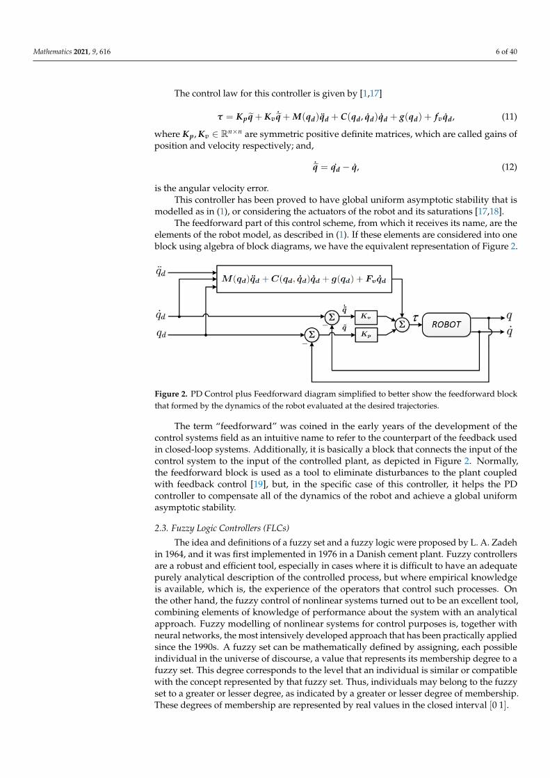
elements of the robot model, as described in (1). If these elements are considered into oneblock using algebra of block diagrams, we have the equivalent representation of Figure 2.

Figure 2. PD Control plus Feedforward diagram simplified to better show the feedforward blockthat formed by the dynamics of the robot evaluated at the desired trajectories.

The term “feedforward” was coined in the early years of the development of thecontrol systems field as an intuitive name to refer to the counterpart of the feedback usedin closed-loop systems. Additionally, it is basically a block that connects the input of thecontrol system to the input of the controlled plant, as depicted in Figure 2. Normally,the feedforward block is used as a tool to eliminate disturbances to the plant coupledwith feedback control [19], but, in the specific case of this controller, it helps the PDcontroller to compensate all of the dynamics of the robot and achieve a global uniformasymptotic stability.

2.3. Fuzzy Logic Controllers (FLCs)

The idea and definitions of a fuzzy set and a fuzzy logic were proposed by L. A. Zadehin 1964, and it was first implemented in 1976 in a Danish cement plant. Fuzzy controllersare a robust and efficient tool, especially in cases where it is difficult to have an adequatepurely analytical description of the controlled process, but where empirical knowledgeis available, which is, the experience of the operators that control such processes. Onthe other hand, the fuzzy control of nonlinear systems turned out to be an excellent tool,combining elements of knowledge of performance about the system with an analyticalapproach. Fuzzy modelling of nonlinear systems for control purposes is, together withneural networks, the most intensively developed approach that has been practically appliedsince the 1990s. A fuzzy set can be mathematically defined by assigning, each possibleindividual in the universe of discourse, a value that represents its membership degree to afuzzy set. This degree corresponds to the level that an individual is similar or compatiblewith the concept represented by that fuzzy set. Thus, individuals may belong to the fuzzyset to a greater or lesser degree, as indicated by a greater or lesser degree of membership.These degrees of membership are represented by real values in the closed interval [0 1].

Mathematics 2021, 9, 616 7 of 40

Fuzzy variables facilitate gradual transitions between different states, and they have anatural ability to express and deal with measurement and observation uncertainties. Tradi-tional variables, so-called crisp variables, do not have this ability. Although the definitionof states by crisp sets is mathematically correct, it is not realistic for measurement errors. Ameasurement that falls in a close neighbourhood of the boundary of two different states of avariable is taken as belonging to only one of those states, despite the uncertainty involved.

Fuzzy control rules are the knowledge of an expert in any related field of application.A fuzzy rule is represented by a sequence of the form IF–THEN (IF–THEN), giving riseto algorithms that describe what action or output should be taken in terms of the currentinformation. The design of fuzzy rules is based on the knowledge or experience of anexpert. An IF-THEN fuzzy rule associates a condition using linguistic variables and fuzzysets to an output or a conclusion. The IF part captures the knowledge through the use ofelastic conditions, and the THEN part provides the conclusion or output in the form of alinguistic variable. These IF-THEN rules are used by a fuzzy inference system to calculatethe degree to which the input data matches the condition of a rule [20].

Figure 3 shows the typical block diagram for a Fuzzy Logic Controller (FLC) used indirect form to control a plant.

Figure 3. Block diagram for an FLC used in direct form. The input signals, x, to the FLC are theerrors obatined from the summation point, and their outputs, y are the control signals to the plant.

From inside, an FLC can be represented in a general form, as in [21] Figure 4.

Figure 4. Internal diagram of an FLC showing all the elements that compute its output.

Fuzzy Inference deduces the fuzzy output from the rule base and the input signals.This divides the FLCs into two types that can be distinguished mainly:

Mamdani type, when the rules and their consequences are both defined linguistically;and, T-S-K type (Takagi, Sugeno, and Kang), when the rules and/or their consequences are

Mathematics 2021, 9, 616 8 of 40

in the form of a mathematical function, so they do not use a defuzzification interface andthe inference engine works differently.

For this work, we are mainly interested in the Mamdani type of FLC. When consideringthat the FLC has n inputs x1, x2, . . . , xn and m outputs y1, y2, . . . .ym; these n×m variablesdefine the knowledge base for the FLC, with its IF–THEN rules being of the form,

IF x1 is Al11 AND x2 is Al2

2 . . . AND xN is Alnn THEN yi is Bl1l2 ...ln

i ; i = 1, 2, . . . , m, (13)

with xk ∈ Uk ⊂ R; k = 1, 2, . . . , n where Uk; k = 1, 2, . . . , n are the universes of discoursefor every xk; yi ∈ UOi ⊂ R; i = 1, 2, . . . , m, where UOi are the universes of discourse forevery output yi. Alk

j ⊂ Uk; k = 1, 2, . . . , n; j = 1, 2, . . . Nk, are the fuzzy sets for every xk;

Bl1l2 ...lni ⊂ UOi; i = 1, 2, . . . , m are the fuzzy sets for every output yi. When a lj fuzzy

rule is fired, the function µlkAj(xk), which is called membership function (MF) of xk in Aj,

assigns a value to the membership grade of xk in the fuzzy set Aj; and finally, the outputvariable, y has a MO number of MFs µBl

i(y) that are related to every consequent of the

rule base, µB

l1 l2...lni

(y), where y is the fuzzified output. The total number of fuzzy rules is

calculated as N = N1N2 · · ·Nn, the multiplication of the number of MFs for each input. Forthe defuzzification block that converts the fuzzified output y into a crisp value, there areseveral methods reported in literature [22], from them the most used in the implementationof Mamdani FLCs are the Center of gravity (COG) and the centre average (CA), and,from those two, the CA is of particular interest, since most implementations of FLC usesingletons as output fuzzy sets. With a CA defuzzifier and a minimum inference, everyoutput of our Mamdani FLC is computed as

y =

N1∑

l1=1· · ·

Nn∑

ln=1yl1···ln

n⋂i=1

µliAi(xi)

N1∑

l1=1· · ·

Nn∑

ln=1

n⋂i=1

µliAi(xi)

, (14)

and if the product inference method is used, every output is equal to

y =

N1∑

l1=1· · ·

Nn∑

ln=1yl1···ln

n∏i=1

µliAi(xi)

N1∑

l1=1· · ·

Nn∑

ln=1

n∏i=1

µliAi(xi)

. (15)

Additionally, if the output fuzzy sets are defined as singletons, y is directly the value of thecorresponding singleton without the need to compute the centres of the inferenced output.

3. Sectorial Fuzzy Control Plus Feedforward Compensation

The control objective is to find a motion tracking sectorial fuzzy controller to ensureglobal uniform asymptotic stability of the non-autonomous closed loop system, guaran-teeing that the angular position errors asymptotically tend to zero. Toward this end, wepropose the Sectorial Fuzzy Control plus feedforward, which has a very similar configura-tion as the PD control plus feedforward, as described in [1], except that, in our proposal,the PD control is replaced by a Sectorial Fuzzy Control, as shown in Figure 5. The controllaw for this new control scheme is,

τ =Φ(q, ˙q)+ M(qd)qd + C(qd, qd)qd + g(qd) + Fvqd, (16)

where Φ(q, ˙q)

is a n× 1 vector whose elements φi(qi, ˙qi), with i = 1, 2, 3, . . . , n, are the realinput–output mappings of the n SFCs,

Mathematics 2021, 9, 616 9 of 40

Φ(q, ˙q)=

φ1(q1, ˙q1)φ2(q2, ˙q2)

...φn(qn, ˙qn)

. (17)

It has been proven in [23] that a SFC is actually a PD controller, but, in this case,its gains become a nonlinear fuzzy equivalent of the KP and KV gains of a regular PDcontroller via the computation of the function Φ

(q, ˙q). This provides the original PD

control with feedforward compensation with the properties of a fuzzy controller, mainlythe tolerance to slight parametric deviations.

Figure 5. Proposed Sectorial Fuzzy Control plus feedforward. The feedforward block is formed bythe dynamics of the robot evaluated at the desired trajectories, their first and second derivatives. Thecontroller is of a special fuzzy class, named sectorial, due to its sectorial properties, and it performsthe tasks of a PD controller, but as a Mamdani fuzzy system of its own.

3.1. Sectorial Fuzzy Controller (SFC) and Its Properties

First introduced by Calcev in [2], a SFC is a special class of fuzzy controller that formsa nonlinear input–output static mapping relating two inputs to one output, with usefulsectorial properties that enable the analysis of its stability. Because there are two inputsx1, x2 and one output y, these three variables define the knowledge base for the SFC, withits IF–THEN rules being of the form,

IF x1 is Al11 AND x2 is Al2

2 THEN y is Bl1l2 , (18)

with x1 ∈ U1 ⊂ R and x2 ∈ U2 ⊂ R, where U1,U2 are the universes of discourse of x1, x2,respectively; and, taken in tandem, they form a two-dimensional universe of discoursefor the input vector x = [x1x2]: x ∈ U = U1 × U2 ⊂ R2; y ∈ UO ⊂ R, where UOis the universe of discourse of the output y. Al1

1 ⊂ U1, Al22 ⊂ U2, are the fuzzy sets

for x1, x2, respectively; while, Bl1l2 ⊂ UO fuzzy sets for y. When a l1, l2 fuzzy rule isfired, the function µl1

A1(x1), called membership function (MF) of x1 in A1, assigns a value

to the membership grade of x1 in the fuzzy set A1; likewise, the MF µl2A2(x2) assigns a

value to the membership grade of x2 in the fuzzy set A2; and finally, the output variable,y has a odd MO number of MFs µBl (y) related to every consequent of the rule base,

µBl1 l2 (y) ∈ µ−MO−1

2B (y), µ

−MO−12 −1

B (y) . . . , µMO−1

2B (y). In this case, for a fuzzy controller to

be a SFC, it must have an odd number of input and output fuzzy sets, that is M1, M2, andMO must be odd [2], therefore li = −Mi−1

2 ,−Mi−12 + 1, . . . , Mi−1

2 , i = 1, 2, O. The totalnumber of fuzzy rules is calculated as M = M1M2, the multiplication of the number ofMFs for each input. An example of the summarized fuzzy rule base is shown in its look-uptable in Table 1.

Mathematics 2021, 9, 616 10 of 40

A fuzzy controller must defined, as follows, to be a SFC [2–4]: One output as a fuzzymapping of two inputs. All of the MFs have to be symmetric with respect to zero, withan odd number of input and output fuzzy sets. The MF of adjacent input fuzzy sets mustbe defined, so that they have complementary membership grades for every input value.The definition of fuzzy sets for the input MF must be convex in the sense given by [2], andaround zero no trapezoidal or similar MFs can be used, since, for null inputs, there must bea null consequent. The consequents of the fuzzy rules table increase from left to right, andfrom top to bottom, with a null output for null inputs, this creates a diagonal antisymmetryaround the centre of the fuzzy rules table, as it can be exemplified and readily seen inTable 1. The output is computed by the centre average defuzzifier, applying the minimumor product inference method. Because of the condition for |φi(qi, ˙qi)− φi(0, ˙qi)| 6= 0 statedin (42) found within the development of Lemma 3 in the next section, no column orrow adjacent to a zero input row or column can have the same consequents. With all ofthese specifications and lineaments, the output of the SFC is computed as the nonlinearinput–output static mapping relating two inputs to one output, φ(x1, x2), as follows

φ(x1, x2) =

M1−12∑

l1=−M1−1

2

M2−12∑

l2=−M2−1

2

µl1A1(x1)µ

l2A2(x2) yl1,l2

M1−12∑

l1=−M1−1

2

M2−12∑

l2=−M2−1

2

µl1A1(x1)µ

l2A2(x2)

, (19)

if the product inference method is selected, and

φ(x1, x2) =∑

M1−12

l1=−M1−1

2∑

M2−12

l2=−M2−1

2

(µl1

A1(x1)

⋂µl2

A2(x2)

)yl1,l2

∑M1−1

2

l1=−M1−1

2∑

M2−12

l2=−M2−1

2

µl1A1(x1)

⋂µl2

A2(x2)

, (20)

if the minimum inference method is used.

When a SFC is defined as outlined in the previous paragraphs, it will have the nextsectorial properties listed below. All of these properties have already been proven in [2,3].

• Property 1, φ(0, 0) = 0, (null output for null inputs);• Property 2, φi(qi, ˙qi) = −φi(−qi,− ˙qi), (symmetric around the origin);• Property 3, there exist ζi, ρi > 0, such that

0 < qi[φi(qi, ˙qi)− φi(0, ˙qi)] ≤ ρi q2i , (21)

0 < ˙qi[φi(qi, ˙qi)− φi(qi, 0)] ≤ ζi ˙q2i , (22)

which means, in both (21) and (22), that both terms inside the inequalities are positive,and bounded by a quadratic of q, and ˙q, respectively.

• Property 4, φi(qi, 0) = 0⇒ qi = 0, (corollary of Property 1);• Property 5, |φi(qi, ˙qi)| ≤ δ := maxl1 l2 yl1 l2, (the SFC is upper-bounded by a maximum

output value);• Property 6, yk 0 ≤ |φi(qi, 0)| ≤ yk+1 0; (sectorial behaviour of (qi, 0)) for i = 1, 2, 3, . . . , n,

where yl1 l2, yk 0, yk+1 0 represent the centres of the corresponding output MFs that aredefined during the design stage.

For the rest of this work we have selected, without a loss of generalisation, the nextspecifications to define the SFC under study:

• singleton consequents, so that the centres of the corresponding output MFs do not needto be computed in order to decrease the computing time and computing complexity ofour controller. This will enable us to implement it in any low-end real time platform,

Mathematics 2021, 9, 616 11 of 40

• product inference, which will turn (19) into the convex combination of (23) as exploitedpreviously in [3,4], and

• and centre average defuzzifier, which is a prerequisite for our controller to be a SFC.

Applying this specifications to (19), and also considering the n× 1 elements of Φ(q, ˙q)

in (17), letting x1 = qn, x2 = ˙qn in (19), we have that the elements of this vector can becomputed as

φn(qn, ˙qn) =

N1−12

∑l1=−

N1−12

N2−12

∑l2=−

N2−12

µl1A1n

(qn)µl2A2n

( ˙qn) yl1,l2 , (23)

where µl1A1n

(qn) represents the MF, which assigns a value to the membership grade of qn in

the fuzzy set A1n; µl2A2n

( ˙qn) represents the MF, which assigns a value to the membershipgrade of ˙qn in the fuzzy set A2n; and, yl1,l2 is the consequent of the fuzzy rule that has beenfired according to the values of qn, ˙qn.

3.2. New Properties of the SFC

The following lemmas are provided to develop new properties for a SFC that facilitatethe stability proof of the proposed control scheme.

Lemma 1. Consider a neighbourhood Ω = x ∈ R | |x| < ε for some ε > 0. Let f (x) be a C′

differentiable, strictly increasing function of x (on Ω) that satisfies f (0) = 0. Then, there existsβ > 0 ∈ R such that ∫ x

0f (τ)dτ ≥ β tanh2(x),

holds ∀x ∈ Ω, with β < 16 inf f ′(x)

Proof of Lemma 1. Let us define the function

g(x) :=∫ x

0f (τ)dτ − β tanh2(x).

Differentiating g(x), the expression of (24) is obtained, and differentiating again this result,we have the relationship in (25)

dgdx

= f (x)− 2βsech2(x) tanh(x), (24)

d2gdx2 = f ′(x) + 2βsech2(x)

[2 tanh2(x)− sech2(x)

]. (25)

It is possible to verify that the next expression holds

f (0)− 2βsech2(0) tanh(0) = 0,

thus, g(x) has an extrema at x = 0.Next, for (25) to be positive ∀x ∈ Ω, we must have

inf f ′(x)β

> −sech2(x)[4 tanh2(x)− 2sech2(x)

]. (26)

Given that the next lower bound holds for the right hand of (26),

supx∈Ω

−sech2(x)

[4 tanh2(x)− 2sech2(x)

]≤ 6,

Mathematics 2021, 9, 616 12 of 40

it can be established that (26) will be verified if the next bound holds for inf f ′(x):

inf

f ′(x)> 6β

consequently, g(x) is convex and it has a strict local minimum at x = 0. Because g(0) = 0,this implies ∫ x

0f (τ)dτ − β tanh2(x) ≥ 0,

or, in other words, the Lemma has been proven:∫ x

0f (τ)dτ ≥ β tanh2(x)

Lemma 2. Let φ(x1, x2) be defined as in (23) [2–4]. Let µ0A(x) be differentable on a neighbourhood

of the origin, but maybe not at the origin, and µ0A1

’(x) > 0 for x < 0, µ0A1

’(x) < 0 for x > 0.Subsequently, there exists β > 0, such that∫ x

0φ(τ, 0)dτ ≥ β tanh2(x), (27)

holds ∀ x ∈ R, with β < 16 inf f ′(x)

Proof of Lemma 2. Consider a neighbourhood Ω of the origin, as in Lemma 1, close to theorigin, the function φ(x, 0) may be expressed as

φ(x, 0) = y1,0(

1− µ0A1(x))

, (28)

for x > 0, andφ(x, 0) = −y1,0

(1− µ0

A1(x))

, (29)

for x < 0The derivative of (28), on x > 0 is computed as

φ’(x, 0) = −y1,0µ0A1

’(x), (30)

in a similar manner, the derivative of (29) on x < 0 may be expressed as

φ’(x, 0) = y1,0µ0A1

’(x), (31)

due to symmetry, we have that the derivatives of µ0A1

near the origin have the relationship,

µ0A1

’(x−) = −µ0A1

’(x+),

where µ0A1

’(x−) denotes µ0A1

’(x) on x < 0 and µ0A1

’(x+) on µ0A1

’(x) on x > 0. Therefore,from Equations (30) and (31), we can establish that φ’(x, 0) is differentiable at the origin.

Because µ0A1

’(x) < 0 for x > 0 and µ0A1

’(x) > 0 for x < 0, one can conclude fromEquations (30) and (31), that

φ’(x, 0) > 0. (32)

By applying Lemma 1, it can be established that the expression in (33) holds∫ x

0φ(τ, 0)dτ ≥ β tanh2(x), (33)

Mathematics 2021, 9, 616 13 of 40

on a neighbourhood of the origin. Let this neighbourhood be defined by ε = P1i . Themaximum value of φ on Ω is achieved at x = P1j , where this value is given by

γ =∫ P1j

0y1,0(

1− µ0A1(τ))

dτ. (34)

Because yk+1,0 > yk,0, then (33) can be expressed as (35)∫ x

0φ(τ, 0)dτ > γ; x > P1j . (35)

The latter implies that, if γ ≥ β, then (33) holds for x > P1j . Symmetry allows toconclude the same for x < 0. This proves Lemma 2.

Finally, (27) can be represented in the general expression

n

∑i=1

∫ xi

0φ(ξi, 0)dξi ≥ λminB‖tanh (x)‖2, (36)

with B = diagβi, for i = 1, 2, . . . n

Preamble to Lemma 3: Leting x1 = qi and x2 = ˙qi, such that φ(qi, ˙qi) = φ(x1, x2), whereasfollowing the guidelines set forth by [3,4,24] for the definition of fuzzy rules, only fourfuzzy rules and of neighbouring sets can be activated, k and k + 1 for input x1 = qi, and m,m + 1 for input x2 = ˙qi, then the output of the fuzzy block is computed as:

φ(x1, x2) = µkA1(x1)µ

mA2(x2)yk,m + µk+1

A1(x1)µ

mA2(x2)yk+1,m

+ µkA1(x1)µ

m+1A2

(x2)yk,m+1 + µk+1A1

(x1)µm+1A2

(x2)yk+1,m+1, (37)

where µkA1(x1), µk+1

A1(xm) represent the k, k+ 1 MF, which assigns a value to the membership

grade of x1 in the fuzzy set A1; µmA2(x2), µm+1

A2(x2) represent the m, m + 1 MF, which assigns

a value to the membership grade of x2 in the fuzzy set A2; and, yk,m, yk+1,m, yk,m+1, yk+1,m+1

represent the consequents of the fuzzy rules being fired.Consider the difference

d(x1, x2) = φ(x1, x2)− φ(0, x2). (38)

The function d(x1, x2) may be written in terms of the membership functions and the fuzzyrules table as

d(x1, x2) = µkA1(x1)µ

mA2(x2)yk,m + µk+1

A1(x1)µ

mA2(x2)yk+1,m

+ µkA1(x1)µ

m+1A2

(x2)yk,m+1 + µk+1A1

(x1)µm+1A2

(x2)yk+1,m+1

− y0,m+1 − µmA2(x2)

(y0,m − y0,m+1

).

Now, consider x1 = x∗1 , where x∗1 => 0 is positive and close to the origin, such thatk = 0.

Evaluating d(x1, x2) at x1 = x∗1 , we obtain

d(x∗1 , x2) = µ0A1(x∗1)µ

mA2(x2)y0,m + µ1

A1(x∗1)µ

mA2(x2)y1,m + µ0

A1(x∗1)µ

m+1A2

(x2)y0,m+1

+ µ1A1(x∗1)µ

m+1A2

(x2)y1,m+1 − y0,m+1 − µmA2(x2)

(y0,m − y0,m+1

).

Next, let y0 = y0,m = y1,m, y1 = y0,m+1 = y1,m+1. Subsequently, by using the fact that

µnAi(xi) + µn+1

Ai(xi) = 1, (39)

Mathematics 2021, 9, 616 14 of 40

we may transform d(x1, x2) into the expression given in (40)

d(x∗1 , x2) = µmA2(x2)y0

[µ0

A1(x∗1) + µ1

A1(x∗1)

]+ µm+1

A2(x2)y1

[µ0

A1(x∗1) + µ1

A1(x∗1)

]− y1 − µm

A2(x2)[y0 − y1]. (40)

By computing all the multiplications in (40) and simplifying, we obtain (41)

d(x∗1 , x2) =µmA2(x2)y0 + µm+1

A2(x2)y1 − y1 − µm

A2(x2)[y0 − y1]

=µmA2(x2)y0 +

(1− µm

A2(x2)

)y1 − y1 − µm

A2(x2)[y0 − y1] = 0, (41)

which implies that, if y0,m = y1,m and y0,m+1 = y1,m+1, then d(x∗1 , x2) is equal to zero forall values of x1 for which k = 0 and all values of x2. The same may be shown to be true ify−1,m = y0,m and y−1,m+1 = y0,m+1. For large values of x2, when m+ 1 = M, µM−1

A2(x2) = 0

and µMA2

= 1. From (40), it is possible to see that only one restriction is needed for d(x∗1 , x2)

to be zero: either y−1,M = y0,M or y0,M = y1,M.

Lemma 3. Consider the function φ(x1, x2). Let the conditions from the previous paragraphs besatisfied, e.g.,

y0,m 6= y1,m, y0,m+1 6= y1,m+1, y−1,m 6= y0,m, y−1,m+1 6= y0,m+1, (42)

suppose that the MF µ01(x1) is differentiable in the intervals P1,0 < x1 < P1,1 and P1,−1 < x1 <

P1,0, and the absolute value of its derivative |µ0 ′1 (x1)| is lower bounded by a constant ϕ, where

P1,k; k : −M . . . M denotes the support values of the MFs for the fuzzy set corresponding to x1,and define

α = ϕ

∣∣∣∣∣ min−M<m<M

y1,m − y0,m, y1,m+1 − y0,m+1, y0,m − y−1,m, y0,m+1 − y−1,m+1∣∣∣∣∣. (43)

Therefore, it holds true that

|φ(x1, x2)− φ(0, x2)| ≥ α|tanh(x1)|. (44)

Proof of Lemma 3. First, consider the interval I1 = [P1,0, P1,1], x1 ∈ I1, k = 0, that is, thefirst interval where |µ0 ′

1 (x1)| exists for positive x1. Let

∆(x1, x2) = φ(x1, x2)− φ(0, x2), (45)

and consider a fixed value of x2, namely x2 = x∗2 . The function ∆(x1, x2) becomes adifferentiable function of x1 on I1. By applying the Mean Value Theorem, there must exista C ∈ I1, such that,

∆(x1, x∗2)− ∆(0, x∗2) =d

dx1(∆(x1, x∗2))

∣∣∣∣x1=C

(x− 0) (46)

since ∆(0, x∗2) = φ(0, x∗2)− φ(0, x∗2) = 0, (46) becomes

∆(x1, x∗2) =d

dx1(∆(x1, x∗2))

∣∣∣∣x1=C

x (47)

The derivative of ∆(x1, x∗2) may be computed, as follows

Mathematics 2021, 9, 616 15 of 40

∆′x1=

ddx1

(∆(x1, x∗2))

=µm2 (x∗2)

[µ0 ′

1 (x1)y1,m − µ0 ′1 (x1)y0,m

]+ µm+1

2 (x∗2)[µ0 ′

1 (x1)y1,m+1 − µ0 ′1 (x1)y0,m+1

]=µ0 ′

1 (x1)(

µm2 (x∗2)

[y1,m − y0,m

]+ µm+1

2 (x∗2)[y1,m+1 − y0,m+1

]),

which satisfies the lower bound expressed in terms of the y as,

∣∣∆′x1

∣∣ ≥ ϕ

∣∣∣∣ min−M<m<M

y1,m − y0,m, y1,m+1 − y0,m+1∣∣∣∣︸ ︷︷ ︸

α1

. (48)

Subsequently, from (47) it can be verified that

|∆(x1, x∗2)| ≥ α1|x1| ≥ |tanh(x1)|. (49)

A similar argument allows for us to state the same for the interval I2 = [P1,−1, P1,0],then it holds that ∣∣∆′x1

∣∣ ≥ ϕ

∣∣∣∣ min−M<m<M

y0,m − y−1,m, y0,m+1 − y−1,m+1∣∣∣∣︸ ︷︷ ︸

α2

, (50)

then, we can make the following definition that encompasses all of the values of the αi withi = 1, 2

α = minα1, α2, (51)

which would lead us to the result on the interval I = I1 ∪ I2 that the lower bound holds forall values of x1. Let us denote, as Dmax, the maximum value of ∆(x1, x∗2) on I. Because, byassumption and design, y1,m > y0,m, the maximum value will be attained at P1,1, which isy1,m+1 > y0,m+1,

Dmax = µm2 (x∗2)

[y1,m − y0,m

]+ µm+1

2 (x∗2)[y1,m+1 − y0,m+1

]. (52)

On the next intervals, for k ≥ 1, the minimum value of ∆(x1, x∗2), denoted as Dmin,can be found to be

Dmin = µm2 (x∗2)

[yk,m − y0,m

]+ µm+1

2 (x∗2)[yk,m+1 − y0,m+1

]. (53)

Because yk,m ≥ y1,m and yk,m+1 ≥ y1,m+1 for k ≥ 1, then, ∆(x1, x∗2) ≥ Dmax for x1 ∈[P1,1, ∞). Since |tanh(x1)| ≤ 1, and then the bound

|∆(x1, x∗2)| ≥ |tanh(x1)|, (54)

holds for all x1 ≥ 0. The argument to show that the bound holds for x1 ≤ 0 is identical.Finally, because the result was shown for any arbitrary value of x2, it holds that.

|φ(x1, x2)− φ(0, x2)| ≥ α|tanh(x1)| (55)

The output of the fuzzy block is computed, once simplified, i:

φ(x1, x2)− φ(0, x2) =[yk,m − y0,m

]+ µk+1

A1’(x1)

[yk+1,m − yk,m

]︸ ︷︷ ︸

monotonic slope

(x1 − P1,k) (56)

Mathematics 2021, 9, 616 16 of 40

that for triangular or trapezoidal MFs, which we are using in this paper, this equationrepresents a set of connecting lines that start at P1,k, on x1, as the abscissa, and

[yk,m − y0,m

]as the ordinate, as shown in Figure 6.

Figure 6. φ(x1, x2) – φ(0, x2) with x2 evaluated at every partition value Pk.

In Figure 7, we can observe a 3-dimensional (3D) representation of the first part of(55) for a wider array of values of x1 and x2, where, in Figure 8, the same 3D plot isviewed only from the perspective of x1. In the latter figure, we can corroborate that if wefollow the guidelines given in the last section for the definition of the SFC’s MFs and itsfuzzy rules table, we will have, as a result, the relationship that is given by (55), where|φ(x1, x2)− φ(0, x2)| can be lower bounded by a |sat(x1)| or a |tanh(x1)| function.

Figure 7. 3D representation of φ(x1, x2) – φ(0, x2).

Mathematics 2021, 9, 616 17 of 40

Figure 8. 3D representation of φ(x1, x2) – φ(0, x2) viewed from the x1 plane.

Finally, (55) can be represented in the more general expression,

‖Φ(x1, x2)−Φ(0, x2)‖ ≥ miniαi‖tanh (x1)‖ (57)

Corollary 1 (Corollary 1 to Lemma 3). From (21) (Property 3 of a SFC), we can conclude that,

sign(Φ(x1, x2)−Φ(0, x2)) = sign(x1), (58)

since, also sign(tanh(x1)) = sign(x1) holds, the first side of (21) can be rewritten as

tanh(x1)[φi(x1, x2)− φi(0, x2)] > 0, (59)

or in vector notation we can express (59) as

tanh (x1)T [Φ(x1, x2)−Φ(0, x2)] > 0 (60)

applying (57) to (60), in vector notation, we have the following relationships

tanh (x1)T [Φ(x1, x2)−Φ(0, x2)] ≥tanh (x1)

T A tanh (x1) ≥λminA‖tanh (x1)‖2 > 0 ∀x1 6= 0 ∈ Rn (61)

with A = diag(αi).

Corollary 2 (Corollary 2 to Lemma 3). From (55), if x2 = 0, we have

|φi(x1, 0)| ≥ αi|tanh(x1)| (62)

which, in a general expression, (62) can be written as

‖Φ(x1, 0)‖ ≥ λminA‖tanh (x1)‖. (63)

Mathematics 2021, 9, 616 18 of 40

Additionally, from (22) in Property 3, stated before for a SFC, evaluating qi = 0,we have

|φi(0, ˙qi)| ≤ ζi| ˙qi|, (64)

extrapolating (64) to the vector-matrix case, it leads to

‖Φ(0, ˙q)‖ ≤ λMaxZ‖ ˙q‖, (65)

where Z = diagζi for i = 1, 2, . . . n.

4. Stability Analysis of the SFC Plus Feedforward Compensation4.1. Closed-Loop Equation

The closed-loop equation of the system represented in the diagram that is shown inFigure 5 is obtained by first neglecting the Coulomb friction term, and second by combining(1) and (2) with the control law defined in (16), as

M(q)q + C(q, q)q + g(q) + Fvq = Φ(q, ˙q)+ τd (66)

with,τd = M(qd)qd + C(qd, qd)qd + g(qd) + Fvqd (67)

and simplifying, in matrix form, the closed-loop system is given by

ddt

[q˙q

]=

[ ˙qM(q)−1(−Φ

(q, ˙q)− C(q, q) ˙q− Fv ˙q− h(q, ˙q)

)]. (68)

The equilibrium points of (68) are defined by

q ∈ Rn : 0 = Φ(q, 0)+ h(q, 0), and ˙q = 0 ∈ Rn (69)

where the origin is an equilibrium point.

Theorem 1. The origin of the state space,[q, ˙q], is a globally uniformly asymptotically stable

equilibrium of the closed loop system that is defined by (68), if the following conditions are met:

λminA > kh2 +(kh2 + γ[λMaxZ+ λmaxFv+ kh1 + kC1‖qM‖])2

4γ(λminFv − γ

[√nkC1 − λmaxM

]− kh1

) (70)

λminFv > γ(√

nkC1 + λmaxM)+ kh1 (71)

0 < γ <

√λminMλminB

λmaxM . (72)

Proof of Theorem 1. We will be applying the direct Lyapunov theorem for non-autonomoussystems in order to carry out the stability analysis. As a first step, we propose the followingLyapunov function candidate (LFC),

V(q, ˙q, t) =12

˙qT M(q) ˙q +n

∑i=1

∫ qi

0φ(ξi, 0)dξi + γ tanh (q)T M(q) ˙q, (73)

with γ > 0, a positive scalar of an enough small arbitrary value.This LFC was proposed based in the guidelines given in [25], in which a Lyapunov

function for mechanical systems is usually constructed using mainly a linear combinationof some kinetic and potential energy functions of the system with a cross-term involving thevariables used in those previous functions. Additionally, the Lyapunov functions describedin [3,4] were used as the references.

Mathematics 2021, 9, 616 19 of 40

As a second step, we need to prove that our LFC is both radially unbounded anddecrescent. To prove the radially unbounded property, we first split the integral term of(73) into two halves, and, applying (36), the result of Lemma 2, to the second half, and alsothe bound properties for the inertia matrix in (3), we have the inequality

V(q, ˙q, t) ≥ 12

λminM‖ ˙q‖2 +12

( n

∑i=1

∫ qi

0φ(ξi, 0)dξi + λminB‖tanh (q)‖2

)− γλmaxM‖tanh (q)‖‖ ˙q‖. (74)

Focussing our attention on the summation-integral term of (74), and using (55) fromLemma 3, we can develop the following relationships,

n

∑i=1

∫ qi

0φ(ξi, 0)dξi ≥

n

∑i=1

αi

∫ qi

0tanh(ξi)dξi, (75)

where, integrating the right-hand side of (75), we have

n

∑i=1

αi

∫ qi

0tanh(ξi)dξi =

n

∑i=1

αi|ln(cosh(qi))|, (76)

therefore, applying the result of(76) in (75), we can write

n

∑i=1

∫ qi

0φ(ξi, 0)dξi ≥

n

∑i=1

αi|ln(cosh(qi))|. (77)

Substituting (77) in (74) and organizing in quadratic form,

V(q, ˙q, t) ≥ 12

([‖tanh (q)‖‖ ˙q‖

]T

Q1

[‖tanh (q)‖‖ ˙q‖

]+

n

∑i=1

αi|ln(cosh(qi))|)

, (78)

with the matrix Q1 defined as

Q1 =

[λminB −γλmaxM−γλmaxM λminM

]. (79)

By applying Sylvester’s theorem, Q1 will be positive-definite if λminB > 0, which isalready fulfilled, since B > 0 in its definition, and if

det(Q1) = λminMλminB − γ2λmaxM2 > 0, (80)

holds. Hence, from the expression computed in (80), γ is obtained as

0 < γ <

√λminMλminB

λmaxM , (81)

this value of γ ensures global positive definiteness and radially unboundedness of (73),since, for ‖ ˙q‖ → ∞, or ‖q‖ → ∞, the right hand of (78) will tend to infinity due to Q1 fromSylvester’s theorem, and that ∑n

i=1 αi|ln(cosh(qi))| → ∞, qi → ∞.Following similar steps to prove that V(q, ˙q, t) is a decrescent function, we now

apply (21), Property 3 of a SFC, to the whole integral term of (73),∫ qi

0φ(ξi, 0)dξi ≤ ρi

∫ qi

0ξidξi

≤ ρi2

q2i , (82)

Mathematics 2021, 9, 616 20 of 40

(82) holds for both positive and negative values of qi, since the integration is performedin the sense of the variable itself. Applying the bound properties for the inertia matrixin (3) and the result from (82) to (73), we can write

V(q, ˙q, t) ≤ 12

[λmaxM‖ ˙q‖2 + λmaxRo‖q‖2

]+γλmaxM‖q‖‖ ˙q‖. (83)

In this case, the right-hand side of (83) will tend to infinity, as any of ‖q‖ or ‖ ˙q‖ tend toinfinity, which means that V(q, ˙q, t) is upper-bounded and, therefore, it is a decrescentfunction. In conclusion, (73) is a globally positive definite radially unbounded decrescentfunction.

As a third step for applying the direct Lyapunov theorem, we obtain the time deriva-tive of the LFC on the trajectories of (68) by applying the Leibniz rule for the differentiationof integrals,

V(q, ˙q, t) = ˙qT M(q) ¨q +12

˙qT M(q) ˙q + Φ(q, 0)T ˙q + γ[sech2(q) ˙q

]TM(q) ˙q

+ γ tanh (q)T M(q) ˙q + γ tanh (q)T M(q) ¨q. (84)

Substituting ¨q from (68), applying the properties of the centrifugal and Coriolis torquematrix that are defined in (5) and (6), and simplifying,

V(·) =− ˙qT[Φ(q, ˙q)−Φ(q, 0)

]− ˙qT Fv ˙q− γ tanh (q)T Fv ˙q− ˙qT h(q, ˙q)

− γ tanh (q)T h(q, ˙q) + γ tanh (q)T CT(q, ˙q) ˙q

+ γ ˙qTsech2(q)M(q) ˙q− γ tanh (q)T Φ(q, ˙q). (85)

Applying the bounds that are defined in (4), (10), and the properties defined in (61)and (65) to simplify (85), we have,

V(·) ≤ − ˙qT[Φ(q, ˙q)−Φ(q, 0)

]− γ(λminA − kh2)‖tanh (q)‖2

− γ

(λminFv − kh1

γ−√

nkC1 − λmaxM)‖ ˙q‖2

+ γ

(λmaxZ+ λmaxFv+

kh2γ

+ kh1 + kC1‖qM‖)‖tanh (q)T‖‖ ˙q‖. (86)

By defining the following constants to simplify the expression in (86),

a = λminA − kh2, b = kh2, (87)

c = λMaxZ+ λmaxFv+ kh1 + kC1‖qM‖, (88)

d = λminFv − kh1, e =√

nkC1 + λmaxM, (89)

substituting them in (86), and rewriting it into a quadratic expression, we have

V(q, ˙q, t) ≤ − ˙qT[Φ(q, ˙q)−Φ(q, 0)

]− γ

[‖tanh (q)‖‖ ˙q‖

]T a −

bγ +c

2

−bγ +c

2dγ − e

︸ ︷︷ ︸

Q2

[‖tanh (q)‖‖ ˙q‖

]. (90)

Since Property 3 of SFCs holds for the first term of V, then if Q2 > 0 =⇒ V(q, ˙q, t) < 0.Therefore, when applying the Sylvester theorem, we have the following relationships

Mathematics 2021, 9, 616 21 of 40

λminA >kh2 =⇒ a > 0,

λminFv >γ(√

nkC1 + λmaxM) + kh1 =⇒ dγ− e > 0,

det(Q2) >0,

where the determinant of Q2 is computed as,

det(Q2) = a(

dγ− e)−

(bγ + c

)2

4> 0. (91)

Obtaining λminA from (87) and (91), we obtain:

λminA > kh2 +(kh2 + γ[λMaxZ+ λmaxFv+ kh1 + kC1‖qM‖])2

4γ(λminFv − γ

[√nkC1 − λmaxM

]− kh1

) . (92)

If λminA complies with (92), then Q2 > 0, therefore, V < 0, which completes the prooffor Theorem 1.

4.2. Sensitivity Analysis

Because we have proven that the our Lyapunov candidate function is a Strict LyapunovFunction, the proposed control law can be properly tuned to account for variations inthe parameters of the controlled system. The sensitivity to parametric variation may beanalysed through Corollary 4.2 of [26] in order to show that some convergence propertiesare preserved.

To this end, parametric variation in the dynamical model is represented as follows.The inertia matrix M(q) may be written as M(q) = M0(q) + ∆M(t) where M0 is thenominal or estimated value of the inertia matrix and ∆M is a matrix containing the errorsinduced by parametric variation for each element of M. Similarly, it is possible to defineC(q, q)q = C0(q, q)q + ∆C(t), g(q) = g0(q) + ∆g(t) and Fv = Fv0 + ∆Fv for the otherterms of the dynamical model (1).

Analogously to the definition of the residual dynamics, the following function is defined:

∆h(t) = −∆Mqd − ∆Cqd − ∆g − ∆Fvqd. (93)

Now, a boundedness assumption is established on ∆h to analyse the sensitivity of theclosed-loop system to the effects of parametric variation.

Assumption 1. There exists a constant k∆h > 0, such that ‖∆h(t)‖ < k∆h for all t ≥ 0.

The existence of k∆h may follow directly from the assumption that each term of (93) isbounded. Therefore, if the bounds for ∆M, ∆C, ∆g and ∆Fv are known, then k∆h can becomputed as

k∆h > k∆M‖qd‖M + k∆C‖qd‖M + k∆g + k∆Fv‖qd‖M, (94)

where k∆M, k∆C, k∆g , k∆Fv > 0 are the upper bounds for each variation term and‖qd‖M, ‖qd‖M represent the upper bounds on the desired joint velocity and acceleration,respectively.

If the control law in (16) is designed while using the nominal values, i.e. with thematrices having sub-index 0, the closed-loop system may be rewritten, as follows,

ddt

[q˙q

]=

[ ˙qM(q)−1(−Φ

(q, ˙q)− C(q, q) ˙q− Fv ˙q− h0(q, ˙q)

)]+ [ 0−M(q)−1∆h(t)

](95)

Mathematics 2021, 9, 616 22 of 40

The first term of (95) will be referred to as the nominal system and the second term ofthe sum as the perturbing term. The nominal residual dynamics term h0(q, ˙q) is the sameas the one that is given in (10), with the difference that the involved matrices are withsubindex 0. Therefore, the existence of constants kh1 and kh2 for the term h0(q, ˙q) also hold.This implies that the stability analysis using (73) as a Lyapunov function still holds for thenominal system.

Consider a domain Dr = w ∈ R2n : ‖w‖ ≤ r, where w = [‖q‖ ‖ ˙q‖]T . On Dr, thelower bound (78) of the Lyapunov function may be written as

V ≥ 12

[‖q‖‖ ˙q‖

]T

Q1D

[‖q‖‖ ˙q‖

]≥ 1

2λminQ1D‖w‖2, (96)

with Q1D given by the expression in (97)

Q1D =

[ε2λminB −γλMaxM−γλMaxM λminM

], (97)

and ε = tanh(r)r is a positive constant that depends on the size of Dr. The fact that ‖q‖ ≥

‖tanh(q)‖ ≥ ε‖q‖ on Dr was also used. The matrix Q1D will be positive definite if

γ < ε

√λminMλminB

λMaxM . (98)

The upper bound of V(·) that is given in (83) may be rewritten as

V(·) ≤ 12

wTQ3Dw ≤ 12

λMaxQ3D‖w‖2, (99)

where Q3D is computed, as in (100)

Q3D =

[λMaxRo γλMaxMγλMaxM λMaxM

]. (100)

It can be shown that the time derivative of (73) along the solutions of (95) satisfies

V(·) ≤ −γ

[‖tanh(q)‖‖ ˙q‖

]T

Q2

[‖tanh(q)‖‖ ˙q‖

]+ λMaxM−1k∆h‖ ˙q + γtanh(q)‖, (101)

with Q2, as given in the stability proof of the nominal system. The term λMaxM−1k∆h‖ ˙q+γtanh(q)‖ appears due to the effect of the perturbing term and, by the triangle inequalityand norm equivalence, it holds that

λMaxM−1k∆h‖ ˙q + γtanh(q)‖ ≤ λMaxM−1k∆h(‖ ˙q‖+ γ‖q‖) (102)

≤√

2λMaxM−1k∆h maxγ, 1‖w‖. (103)

The first term of (101) may be upper bounded by

− γ

[‖tanh(q)‖‖ ˙q‖

]T

Q2

[‖tanh(q)‖‖ ˙q‖

]≤ −γwTQ2Dw ≤ −γλMaxQ2D‖w‖2, (104)

on Dr, with Q2D given in the the definition of (105)

Q2D =

ε2a −bγ +c

2

−bγ +c

2dγ − e

. (105)

Mathematics 2021, 9, 616 23 of 40

The symmetric matrix Q2D will be positive definite if

ε2a(

dγ− e)>

(bγ + c

)2

4, (106)

which holds if the bound defined for λminA in (107) also holds

λminA > kh2 +(kh2 + γc)2

4ε2γ(λminFv − γ[√

nkC1 − λMaxM − kh1 ]). (107)

Consequently, from (101), it can be stated that the derivative of the Lyapunov functionis given by

V ≤ −γλminQ2D‖w‖2 +√

2λMaxM−1k∆h maxγ, 1‖w‖, (108)

which implies that, V < 0 for ‖w‖ >√

2λMaxM−1k∆h maxγ,1γλminQ2D

. By Corollary 4.2 of [26],solutions of (95) are uniformly ultimately bounded and they satisfy

lim supt→∞

‖w‖ ≤ ksup, (109)

with ksup defined in (110), where we have applied all of the definitions for Q1D , Q2D and Q3D

ksup =

√2λMaxM−1k∆h maxγ, 1

γλminQ2D

√λMaxQ3DλminQ1D

. (110)

In summary, for any initial condition of the closed-loop system, with a suitable tuningof the gains for the given initial condition, the solutions converge to a domain that growsaccording to (109). Notice that the domain to which the solutions converge becomes smalleras k∆h, which represents the magnitude of the parametric variation, becomes smaller. Ifk∆h = 0, then uniform asymptotic stability is recovered.

When analysing the result of (110), given its complexity, it is very difficult to determinewhich parameter from the robot model the whole control system is more sensitive to.

5. Results5.1. 2-DOF Robot Manipulator Description

A 2-DOF robot manipulator moving in the vertical plane, built in CICESE, México,and located at Instituto Tecnológico de La Laguna, México, as shown in Figure 9, was usedto evaluate the performance of our controller. It consists of two rigid links, high-torquebrushless direct-drive servos with no gear reduction, little backlash, and very small jointfriction. The maximum torque that can be applied to joint 1 is 150 [N–m], and 15 [N–m] forjoint 2, according to the manufacturer [27,28].

The parameter values for this robot are, l1 = 0.450 m, l2 = 0.450 m, lc1 = 0.091 m,lc2 = 0.091 m, m1 = 23.902 Kg, m2 = 3.880 Kg, I1 = 1.266 Kg m2, I2 = 0.093 Kg m2,f v1 = 2.288 N-m s, f v2 = 0.175 N-m s, and g = 9.81 m/s2.

The dynamical model of the robot that is shown in Figure 9 can be expressed asin (1), with

Mathematics 2021, 9, 616 24 of 40

M11(q) = m1l2c1 + m2[l2

1 + l2c2 + 2l1lc2 cos(q2)] + I1 + I2,

M12(q) = m2[l2c2 + l1lc2 cos(q2)] + I2,

M21(q) = m2[l2c2 + l1lc2 cos(q2)] + I2,

M22(q) = m2l2c2 + I2,

C11(q, q) = −m2l1lc2sin(q2)q2,

C12(q, q) = −m2l1lc2sin(q2)[q1 + q2],

C21(q, q) = −m2l1lc2sin(q2)q1,

C22(q, q) = 0,

g1(q) = [m1lc1 + m2l1]g sin(q1) + m2lc2 g sin(q1 + q2),

g2(q) = m2lc2g sin(q1 + q2),

where Mij(q) are the elements of row i : 1, 2, and column j : 1, 2 of the matrix M(q); Cklare the elements of row k : 1, 2 and column l : 1, 2 of the matrix C(q, q); and, g1(q), g2(q)are the elements of vector g. In our controller definition and implementation, only theviscous friction, Fv, is considered. The Coulomb friction, FC, was only taken into accountwithin the robot model in the definition of the MFs for the two SFCs, and for simulationpurposes; and, beyond that, it will be further taken as a disturbance, as was discussed inprevious sections.

g

1Y

2Y

1q

2q

2cl

2l

1l

1cl

1I

1m

2 2,m I

Figure 9. Diagram of the 2-DOF robot manipulator that was used in the experiments.

5.2. Controller Design5.2.1. SFC Plus Feedforward Design

Fuzzy sets for each input of each joint were defined, as shown in Figures 10 and 11.Figure 10 may be deceiving, as it is depicted having fuzzy sets of regular and equidistantshapes; nonetheless, once the real values for the support points of its fuzzy sets havebeen applied, it will look more as Figure 11 (for both, q or ˙q), which has its fuzzy setspictured in a more realistic way, as the definition of the torque output fuzzy sets for eachjoint, as shown in Figure 12, also does. However, checking all Figures 10–12, they aresymmetric around the origin and have an odd number of MFs, as specified in Section 3.1.The MFs for the angular velocity error input for both joints were originally defined, asit is shown for the input of the system in [29], where a multistage intelligent relayingin priority based decision is controlled via a fuzzy inference system, with some gapsin the definition of the sets; however, such gaps contradict the conditions outlined in

Mathematics 2021, 9, 616 25 of 40

Section 3.1, which were corrected via a Genetic Algorithms optimisation, as it is indicatedin the following paragraphs. Singletons were used for the output fuzzy sets in order toexpedite the computation of the SFC when it is implemented in real-time, as was defined inSection 3.1 without a loss of generalisation. The use of singletons in the output fuzzy sets,along with the CA defuzzifier, simplifies the output equation of the SFC from (19) to (23),which saves precious time used in the calculation of the centres of the inferenced output,since the singletons become those values by default. This, in turn, makes the computationfaster and of much less complexity. Additionally, since the SFC is not being used as anapproximator, the losses, which normally occur during the defuzzification process, cannotbe assessed or even considered, because the SFC is a fuzzy system of its own.

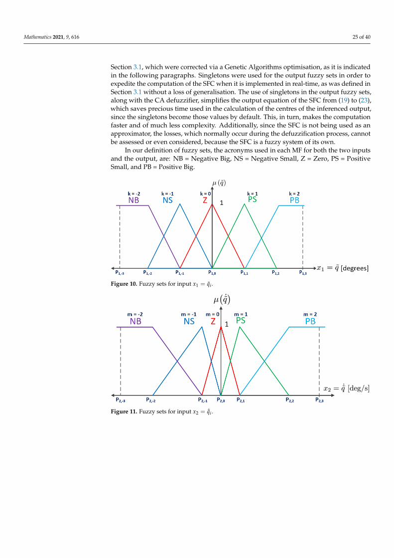
In our definition of fuzzy sets, the acronyms used in each MF for both the two inputsand the output, are: NB = Negative Big, NS = Negative Small, Z = Zero, PS = PositiveSmall, and PB = Positive Big.

Figure 10. Fuzzy sets for input x1 = qi.

Figure 11. Fuzzy sets for input x2 = ˙qi.

Mathematics 2021, 9, 616 26 of 40

Figure 12. Fuzzy sets for output τ.

Table 1 shows the fuzzy rules. They were defined following the guidelines outlined inSection 3, so that the SFC part of our control scheme does have sectorial properties.

Table 1. Fuzzy rules look-up table.

˙q/q l1 = −2 l1 = −1 l1 = 0 l1 = 1 l1 = 2NB NS Z PS PB

l2 = −2NB NB NB NS Z Z

l2 = −1NS NB NB NS Z Z

l2 = 0Z NS NS Z PS PS

l2 = 1PS Z Z PS PB PB

l2 = 2PB Z Z PS PB PB

For the definition of the partition values of the fuzzy, there exists several previousworks like the one in [30], where the algorithm developed by Ishibuchi [31] to automaticallygenerate the number of fuzzy rules along with the fuzzy sets and its partition values isimplemented with the hybrid cooperative Genetic Compilation-Competitive Learning(GCCL) algorithm and the Pittsburgh algorithm (FH.GBML) in order to forecast the powerlevel that is available for a photovoltaic plant; or, the one described in [32], where theprocess of selecting the partition values is turned into an optimisation of distances insideunit hypercubes for a clustering of airports application. However, we used a simplifiedversion of such approaches applying Genetic Algorithms (GA), as in [33], since, due tothe guidelines given to design a SFC, almost all of the work of defining both the fuzzysets and fuzzy rules has already been done. The 2-DOF robot manipulator from Figure 9was used as our plant, where both viscous and Coulomb friction were included within itsmodel, used in the ensuing simulations that are required for the optimisation process. Allof the partition values that define the fuzzy sets for both joints were found in this way. Thesupport values for the fuzzy sets obtained via GA are: P1,0 = 0, P1,1 = 6.518, P1,2 = 53.77,P1,3 = 125.5, P2,0 = 0, P2,1 = 122.2, P2,2 = 138.5 P2,3 = 871.8, Y0 = 0, Y1 = 82.29, Y2 = 204.5,for joint 1; and, P1,0 = 0, P1,1 = 5.982, P1,2 = 36.67 P1,3 = 163.5, P2,0 = 0, P2,1 = 153.8,P2,2 = 318.7 P2,3 = 1016, Y0 = 0, Y1 = 15, Y2 = 180, for joint 2.

The beauty of this control scheme is that is rather easy to both design and implement.Once the fuzzy sets and the fuzzy rules are completely defined, the controller is fullydesigned and ready to be implemented, which only consists of the evaluation of the rules

Mathematics 2021, 9, 616 27 of 40

through IF-THEN code statements, but it delivers a controller that provides amazing results.The latter is the beauty of using this type of controllers.

5.2.2. PD Plus Feedforward Controller Design

We also designed a PD plus feedforward controller to comparatively test its per-formance versus that of the SFC plus feedforward. The elements of the gain matricesKp, Kv ∈ R2×2 were obtained while using the same optimising method of GA, as in thecase of the SFC, but adapted to a PD case. This optimisation yielded the values:

Kp = diag70.7137, 9.5283 Kv = diag16.1162, 4.377.

5.3. Comparative Simulation

The SFC plus feedforward was simulated in comparison with its classic crisp coun-terpart, the PD plus feedforward controller. Both of the controllers were simulated inMATLAB/Simulink R2015a using an ode5 (Dormand-Prince) solver algorithm with afixed step of 2.5 ms. The 2-DOF robot from Figure 9 was used as the plant, first, whileconsidering the same hypothetical assumption used in the definition of the SF+ff controllaw and its stability analysis: that is, the Coulomb friction is non-existent. The desiredposition, velocity, and joint acceleration trajectories qd(t), qd(t), and qd(t), are given by thenext equations, according to the values and functions given in [34] in order to demand themaximum allowable performance for this specific robot:

q1d(t) = a1 + b1(1− e−d1t3) + c1(1− e−d1t3

) sin(ω1t) [rad], (111)

q2d(t) = a2 + b2(1− e−d2t3) + c2(1− e−d2t3

) sin(ω2t) [rad], (112)

where a1 = π/2 [rad], b1 = π/4 [rad], c1 = π/18 [rad], d1 = 2, ω1 = 15 [rad/s], a2 = π/2[rad], b2 = π/3 [rad], c2 = 25π/36 [rad], d2 = 1.8, and ω2 = 3.5 [rad/s. from thedesired positions, the desired velocities, and accelerations were analytically computedby calculating their derivatives. Additionally, the comparative responses of the desiredtrajectories versus the actual angular position, the angular errors, as well as the appliedtorques in each joint were obtained, as shown in Figures 13–18, respectively.

Figure 13. Desired vs. actual position in joint 1, without Coulomb friction.

Mathematics 2021, 9, 616 28 of 40

Figure 14. Desired vs. actual position in joint 2, without Coulomb friction.

Figure 15. Angular Position error for joint 1, without Coulomb friction.

Figure 16. Angular position error for joint 2, without Coulomb friction.

Mathematics 2021, 9, 616 29 of 40

Figure 17. Applied torque to joint 1, without Coulomb friction.

Figure 18. Applied torque to joint 2, without Coulomb friction.

The results of Figures 15 and 16 corroborate that, for both the PD plus feedforwardand the SFC plus feedforward, q = [q1 q2]

T show an asymptotic uniform response, asstated by their stability analysis. All of this while bounded torques are held at all times.

A comparison of the angular position error RMS for each joint is given for bothcontrollers in Table 2. All of the values are RMS. We are comparing the total error in thespan of time considered for the simulation, which is 10 s, and the steady-state error, whenconsidering that the steady-state starts at 5 s. The subindex “ss” stands for the steady-statevalues, computed from 5 s to the end of the time window used. Additionally, the PD plusfeedforward is labelled as ‘PD + ff’, and the SFC plus feedforward as ‘SFC + ff’.

Table 2. RMS comparative of the simulation results for q without FC .

Controller q1 q1,ss q2 q2,ss

PD + ff 11.7759 0 16.3671 0.0005SFC + ff 13.5810 0 15.0448 0

The PD plus feedforward achieved a better overall performance in joint 1 due to afaster fuelled by a higher torque supplied at start-up compared to the SFC plus feedforward,

Mathematics 2021, 9, 616 30 of 40

which had a softer start-up achieved from the application of the GA to the design of its MFs.Both controllers have a zero steady-state angular position error. On the other hand, forjoint 2 the SFC plus feedforward shows a better response in both analysis: total and steady-state, while the PD plus feedforward has a slight remnant due to a complete exponentialresponse that is still settling at 10 s of elapsed time.

In Table 3 we compare the overall and steady-state torques applied to both joints bythe controllers. Again, the steady-state torques are computed 5 s after start-up, and labelledwith a subindex “ss”.

Table 3. Root Mean Square (RMS) of applied torques comparative of the simulations without FC .

Controller τ1 τ1,ss τ2 τ2,ss

PD + ff 71.8674 72.9388 3.8514 3.4772SFC + ff 72.0708 72.9388 3.8784 3.4772

In steady state, both of the controllers have the same applied torques to the cor-responding joint. Nevertheless, the PD plus feedforward has smaller values of overallapplied torques for both joints, as compared to the SFC plus feedforward. Additionally,the total RMS applied torques are smaller than the steady-state ones for both controllers onboth joints. Since the RMS values measure the density of the signal in the time windowconsidered, in this case the applied torques are denser in steady-state than in the total timeof the simulation.

Table 4 shows a tabulation of the transient-response parameters of the robot with bothcontrollers being applied. For this table, we use the next acronyms:

• maximum overshoot = MP,• rise time = tr, and• settling time = ts.

with a subindex indicating which joint is being considered. NOTE: the transient parameterswere measured directly on the graphic responses and they are an approximation of thereal values.

Table 4. Transient response comparative of the simulation results without FC .

Controller MPq1 trq1tsq1

MPq2 trq2tsq2

PD + ff 6.9908% 0.5057 s 2.2669 s 0% 1.5484 s 2.5328 sSFC + ff 3.9% 0.5660 s 1.11 s 0.387% 0.7251 s 0.87 s

Here, we have a numeric evidence that corroborates the comparative responses thatare shown in Figures 13–16, with the PD plus feedforward having a shorter tr than the SFCplus feedforward, but longer ts and a larger MP in joint 1. While, in joint 2, the SFC plusfeedforward has much better transient and steady-state responses.

Next, the same simulations were carried out, but now considering the hypotheticalfunction and parameters for the Coulomb friction in the robot model, according to themanufacturer [27,28]. Additionally, the comparative responses of the desired trajectoriesversus the actual angular position, the angular errors, as well as the applied torques inevery joint were obtained, as shown in Figures 19–24, respectively.

Mathematics 2021, 9, 616 31 of 40

Figure 19. Desired vs. actual position in joint 1.

Figure 20. Desired vs. actual position in joint 2.

Figure 21. Angular position error in joint 1.

Mathematics 2021, 9, 616 32 of 40

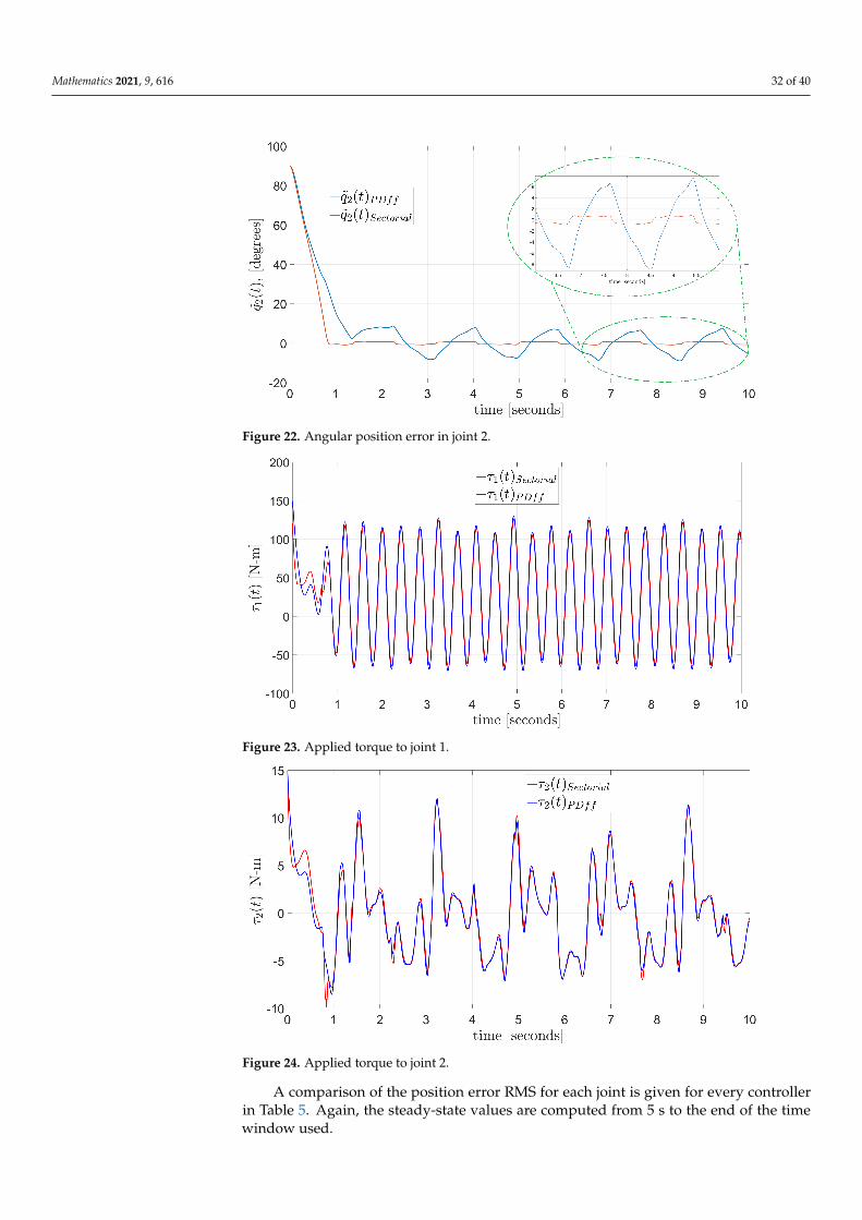
Figure 22. Angular position error in joint 2.

Figure 23. Applied torque to joint 1.

Figure 24. Applied torque to joint 2.

A comparison of the position error RMS for each joint is given for every controllerin Table 5. Again, the steady-state values are computed from 5 s to the end of the timewindow used.

Mathematics 2021, 9, 616 33 of 40

Table 5. Position Error RMS comparative of the simulation results for q with FC .

Controller q1 q1,ss q2 q2,ss

PD + ff 12.0077 0.9923 18.1359 4.8118SFC + ff 14.2844 0.6082 15.8829 0.6476

In general, the position errors have smaller values for the SFC plus feedforward,although the PD plus plus feedforward achieved a better overall performance due to afaster response in joint 1. On the other hand, for that same joint it presented a worsesteady-state error measurement. For both controllers, adding the Coulomb friction createdan error residual that was even worse for the PD plus feedforward in joint 2.

In Table 6, the overall and steady-state torques that are applied to both joints by thecontrollers are tabulated.

Table 6. RMS of applied torques comparative of the simulations with FC .

Controller τ1 τ1,ss τ2 τ2,ss

PD + ff 69.5238 70.0061 4.4055 4.0536SFC + ff 67.2862 68.4302 4.4162 4.0694

Again, as for the simulation without FC, in joint 1, the total RMS applied torques werelower than the ones that were applied in the steady-state phase considered; whilst, for joint2 it was the reverse case. We can see that, with the FC included in the model of the robot, theSFC plus feedforward supplies lower torque and achieves a smaller steady-state angularposition error than the PD plus feedforward in joint 1 (38.71 % of difference). In steady-stateon joint 2, the torque that is applied by the SFC is slightly higher (0.2429%) than the oneapplied by the PD plus feedforward, but the difference in RMS angular position error isvery large (86.54% of difference).

Table 7 shows a comparison of the robot transient-response parameters with bothcontrollers being applied. For this table, we use the same acronyms and labelling as forTable 4. NOTE: the transient parameters were measured directly on the graphic responsesand they are an approximation of the real values.

Table 7. Transient response comparative of the simulation results with FC .

Controller MPq1 trq1tsq1

MPq2 trq2tsq2

PD + ff 0.0821% 0.7 s 2.5 s 8.97% 2.5288 s 2.51 sSFC + ff 0% 0.7294 s 0.8782 s 0% 0.8406 s 1.3823 s

The SFC plus feedforward presents a better transient response performance in almostall parameters, except in the rise time of joint 1, and that again is due to a higher suppliedtorque by the PD plus feedforward at start-up. However, the latter caused a slightlyovershoot compared to a 0% overshoot for the SFC plus feedforward for joint 1.

5.4. Experimental Implementation

The 2-DOF robot shown Figure 9 was used as the plant, now in a physical set ofexperiments. The desired trajectories that are defined in (112) along with their derivativesfor qd and qd were used in the experiments. Both controllers, the SFC plus feedforwardand the PD plus feedforward controller, once designed and simulated, were implementedusing Ansi C on WinMechLab, a real-time platform running on an Intel Pentium 4 PC withreal-time Windows XP [35], with a 2.5 ms sampling period, and using a MultiQ-PCI dataacquisition board from Quanser Consulting Inc. The angular position error responses wereobtained for each joint, as well as the applied torques, as shown in Figures 25–28. The PD

Mathematics 2021, 9, 616 34 of 40

plus feedforward controller had to be retuned eight times in order to mitigate the torqueovershoot that was injected to the robot. After this retuning, its parameters had the values,

Kp = diag70.7137, 41.7283 Kv = diag11.1162, 4.377 (113)

Figure 25. Angular position error for joint 1.

Figure 26. Angular position error for joint 2.

Mathematics 2021, 9, 616 35 of 40

Figure 27. Applied torque to joint 1.

Figure 28. Applied torque to joint 2.

In Table 8, a comparison of the Root Mean Square (RMS) position error in each jointis shown for every controller, and the steady-state values were computed from 5 s to theend of the experiment. Additionally, in Tables 9 and 10, a comparative tabulation of theRMS applied torques to each joint, and the transient response parameters of the robot withthe two controllers applied, are shown. NOTE: the transient parameters were measureddirectly on the graphic responses and they are an intuitive approximation of the real values.

Table 8. RMS Position Error comparative for the experimental implementation.

Controller q1 q1,ss q2 q2,ss

PD + ff 17.1754 1.4021 17.1683 5.3036SFC + ff 15.218 1.1867 15.9701 0.6256

Mathematics 2021, 9, 616 36 of 40

Table 9. RMS of applied torques comparative for the experimental implementation.

Controller τ1 τ1,ss τ2 τ2,ss

PD + ff 66.0457 65.3537 4.4670 4.1095SFC + ff 59.4368 58.6641 4.5628 4.2463

Table 10. Transient response comparative of the experimental results.

Controller MPq1 trq1tsq1

MPq2 trq2tsq2

PD + ff 0.94% 3.6049 s 4.7 s 0% 2.55 s 3.17 sSFC + ff 0% 1.0767 s 1.27 s 0% 0.8646 s 1.3856 s

For all joints, the position errors have smaller values for the SFC plus feedforwardin both the comparative table and figures than for the PD plus feedforward controller(labelled PD + ff). The differences are of 11.4%, 15.36% for the overall RMS angular positionerror and the RMS steady-state angular position error in joint 1, respectively; and, for joint2, of 6.98% for the overall RMS angular position error, and 88.2% RMS steady-state angularposition error. The applied torques in both joints have similar values, as in joint 2, wherethe difference is of 2.14%, or are generally smaller (joint 1 case) for our proposed SFC plusfeedforward. In the case of the transient response parameters, the SFC plus feedforwardhad much shorter rise time (70.3% shorter for joint 1, and 66.09% shorter for joint 2) andsteady-state time (70.26% in joint 1, and 56.29% in joint 2) than the PD plus feedforward.All of this while having a smaller applied torque to joint 1, and a slightly (2.1% overall,3.22% in steady-state) applied torque to joint 2.

6. Discussion

In the hypothetical simulation where the model of the robot is considered withoutCoulomb friction, the uniform asymptotic error response is corroborated for both con-trollers, where both of them present under damped responses in Figure 13 and exponentialor over damped responses in Figure 14. In addition to the SFC plus feedforward showsan amazing, almost instantaneous response. The must puzzling of this observation is that,just for a slight under shoot, both torque responses are almost the same for both controllersin Figure 18. It is necessary to inform that the response obtained in Figures 13 and 14 wasachieved either eliminating the Coulomb friction from the robot model or by including itin the robot model that conforms the feedforward compensation in both controllers.

In simulation, for joint 1, the position error has a smaller value in steady state forthe SFC plus feedforward in both the comparative table and figures than for the PD plusfeedforward controller (labelled PD + ff), while the applied torque is the same at start-up forthe two control schemes, and smaller at steady-state for the SFC plus feedforward. Becausethe rise time in the graph is smaller for the classic counterpart than for the proposed controlscheme, the total error measurement is also lower. Steady-state position error for joint 1looks the same for both control schemes at first sight, however in the zoomed part of Figure21 a wobbling response is observable for the PD + ff controller that also contains a bias thatforces the error to oscillate below zero, while the SFC + ff has a lower peak-to-peak valueand it presents no bias. The latter can be confirmed in the steady-state column of Table 5 forq1. The residual error, as compared to the previous hypothetical response, which is shownin the zooming part of Figure 21, is due to the coulomb friction that is not compensated bythe τd part of the control law, the part corresponding to the desired robot dynamics, since itis unknown and considered to be part of the disturbances.

In the physical experimental test, for joint 1, the position error has a smaller value forthe SFC plus feedforward (labelled as ‘Sectorial’) in both the comparative table and figures,than for the PD plus feedforward controller (labelled PD + ff), while the applied torqueis the same at start-up for the two control schemes, and smaller at steady-state for theSFC plus feedforward. Additionally, the rise time of the graph is smaller for the proposed

Mathematics 2021, 9, 616 37 of 40

control scheme (lees than 1 s) than its classic counterpart. Steady-state position error forjoint 1 looks the same for both control schemes at first sight, however in the zoomedpart of Figure 25 a wobbling response is observable for the PD + ff controller that alsocontains a bias that forces the error to oscillate below zero, while the SFC + ff has a lowerpeak-to-peak value and presents no bias. The latter can be confirmed in the steady-statecolumn of Table 8 for q1. The residual error shown in the zooming part of Figure 26 is dueto the coulomb friction that is not compensated by the τd part of the control law, the partcorresponding to the desired robot dynamics, since it is unknown and considered as partof the disturbances.

In the case of joint 2, for both simulation and experimental test, the difference inthe position error between the two control schemes is very large. While our proposalhas a rise-time of less than 1 s, the classic scheme takes more than 2.5 s to reach the zeroline. The steady-state response differences between the two controllers is abysmal too, asshown in the zoomed part of Figures 22 and 26 and confirmed in Tables 5 and 8 for boththe whole response and its steady-state part. All the latter while having almost identicalapplied torque by both controllers, with the torque applied by the SFC + ff having verysmall differences that nevertheless make a huge difference (see Figures 24 and 28). Again,the residual error shown in the zooming part of the aforementioned figures is due to thecoulomb friction that is not compensated in the control law because it is unknown andtaken as part of the disturbances and unmodelled dynamics.

The seemingly noisy torque applied to joint 2, as shown in Figure 28, is a visual artifactthat is created by the limitations of the platform in which our algorithm is implemented.The sampling period used in our implementations is of 2.5 ms; nevertheless, only twomeasured variables of interest can be delivered in text files by the platform with thesame sampling period, from which we obviously choose q1 and q2. Any other measuredvariable is delivered to us with a sampling rate five to ten times the sampling periodchosen by the users, which is the case for both τ1 and τ2, which are being computed at2.5 ms, but represented at 15 ms in the reporting file, as shown in more detail in Figure 29,which is a magnification of Figure 28. Additionally, the applied torque to both joints (seeFigures 27 and 28) looks more noisy as compared to the ones obtained via simulation (seeFigures 23 and 24) due to some mechanical oscillations that occur during the experiments,and what we see is the controllers performing their duty to maintain a minimum angularposition error.

Figure 29. Magnification of applied torque to joint 2 showing visual artifacts created by using adifferent output delivery sampling period.

While small changes in the robot parameters are very limiting for the PD plus feedfor-ward controller, they are much less limiting for the SFC plus feedforward, as evidentiatedby the differences in the simulations with and without Coulomb friction included in the

Mathematics 2021, 9, 616 38 of 40

robot model. But in general, the must limiting factor for both the PD plus feedforward andthe SFC plus feedforward are the maximum torques that can be applied to each joint ofthe robot; this limits the gain values for the PD. Nonetheless, the definition of the MFs forthe SFC can be adjusted in order to avoid saturated torques for big errors and, at the sametime, increase the gains to have small angular position errors in steady state.

7. Conclusions

A novel SFC plus feedforward, applied to the trajectory tracking of a robot manip-ulator, including the formal details of its stability proof using the Lyapunov theorem fornon autonomous systems, has been presented for the first time. Two new properties ofthe SFC were developed in the lemmas that are included in Section 3.2, which allowedfor us to construct a strict Lyapunov function which leads to prove GUAS of the robotmanipulators in closed-loop with the SFC plus feedforward compensation. Additionally,through that strict Lyapunov function, we were able to analyse the sensitivity of our controlscheme; however, given the complexity of the resulting expression, no assessment couldbe made as to which parameter of the robot model the proposed control system is moresensitive to. We successfully evaluated the new control scheme, both experimentally andwith simulations. When the evaluation neglected the Coulomb friction out of the robotmodel, or this parameter was included in the feedforward compensation on the SFC plusfeedforward or in the PD plus feedforward, we obtained a uniform asymptotic responsewith very short rise and settling times. In the case of the SFC plus feedforward, it did notneed any parameter tuning during the experimental trials, which was not the case with itsPD counterpart, which indeed needed to be tuned several times before achieving a similarresponse to the one that was obtained in simulations, which shows the inherent capacity offuzzy systems to cope with small disturbances and uncertainties. Finally, we are proposinga control scheme that presents the following characteristics:

• bounded output torques in accordance with the limits of the actuators,• very simple to design and implement,• individualized design of the SFC for every joint of the robot,• applicable to any serial robot composed by n−links, with any architecture, and• industrial applications limited to those like welding or painting.

Author Contributions: Conceptualization, V.S. and R.G.-H.; methodology, A.P.-L., V.S. and R.G.-H.;software, A.P.-L. and J.V.-C.; validation, A.P.-L., V.S., R.G.-H. and J.V.-C.; formal analysis, A.P.-L., V.S.and J.V.-C.; investigation, A.P.-L., V.S., R.G.-H. and J.V.-C.; resources, V.S. and R.G.-H.; data curation,A.P.-L.; writing—original draft preparation, A.P.-L.; writing—review and editing, A.P.-L., V.S., R.G.-H.and J.V.-C.; visualization, A.P.-L. and J.V.-C.; supervision, V.S. and R.G.-H.; project administration,V.S. and R.G-H.; funding acquisition, A.P.-L., V.S. and R.G.-H. All authors have read and agreed tothe published version of the manuscript.

Funding: This research was funded in part by Programa para el Desarrollo Profesional Docente(PRODEP-México) under grant ITSON-126 and Tecnológico Nacional de México (TecNM) projects.

Institutional Review Board Statement: Not applicable.

Informed Consent Statement: Not applicable.

Data Availability Statement: All data presented or used in this study is contained within thissame article.

Conflicts of Interest: The authors declare no conflict of interest. The funders had no role in the designof the study; in the collection, analyses, or interpretation of data; in the writing of the manuscript, orin the decision to publish the results.

Mathematics 2021, 9, 616 39 of 40

AbbreviationsThe following abbreviations are used in this manuscript:

3D 3-DimensionalCA Center AverageCOG Center of GravityDOF Degree of FreedomDSP Digital Signal Processorff feedforwardFLC Fuzzy Logic ControllerFPGA Field-Programmable Gate ArrayGA Genetic AlgorithmsGUAS Global Uniform Asymptotic StabilityLFC Lyapunov Function CandidateLMI Linear Matrix InequalityMF Membership FunctionMP Maximum overshootPC Personal ComputerPD Proportional + DerivativePID Proportional + Integral + DerivativeRFWFLNN Recurrent Fuzzy Wavelet Functional Link Neural NetworkRMS Root Mean SquareSFC Sectorial Fuzzy ControllerSS Steady-Statetr rise timeT-S Takagi-Sugenots settling time

References1. Kelly, R.; Santibanez, V.; Loria, A. Control of Robot Manipulators in Joint Space; Springer: London, UK, 2005; pp. 269–2822. Calcev, G. Some remarks on the stability of Mamdani fuzzy control systems. IEEE Trans. Fuzzy Syst. 1998, 6, 436–442. [CrossRef]3. Santibanez, V.; Kelly, R.; Llama, M. Global asymptotic stability of a tracking sectorial fuzzy controller for robot manipulators.

IEEE Trans. Syst. Man Cybern. Part B Cybern. 2004, 34, 710–718. [CrossRef] [PubMed]4. Santibanez, V.; Kelly, R.; Llama, M. A novel global asymptotic stable set-point fuzzy controller with bounded torques for robot

manipulators. IEEE Trans. Fuzzy Syst. 2005, 13, 362–372. [CrossRef]5. Zheng, C.; Su, Y.; Mercorelli, P. A simple fuzzy controller for robot manipulators with bounded inputs. In Proceedings of the 2017

IEEE International Conference on Advanced Intelligent Mechatronics (AIM), Munich, Germany, 3–7 July 2017; pp. 1737–1742.6. Nguyen, V.-A.; Nguyen, A.-T.; Dequidt, A.; Vermeiren, L.; Dambrine, M. LMI-Based 2-DoF Control Design of a Manipulator via

T-S Descriptor Approach. IFAC PapersOnLine 2018, 51, 102–107. [CrossRef]7. Coronado, A.; Peñaloza-Mejía, O.; Estrada-Manzo, V.; Bernal, M. A Comparison of Fuzzy Schemes for Trajectory Tracking on

the Furuta Pendulum. In Proceedings of the Congreso Nacional de Control Automático 2017, Monterrey, Nuevo León, Mexico,4–6 October 2017.

8. Kang, H.B.; Lim, H.-K. Robust H∞ Tracking Controller Design for 3-R Link Robotic Manipulator via Takagi-Sugeno fuzzy form.In Proceedings of the 2019 19th International Conference on Control, Automation and Systems (ICCAS 2019), Jeju, Korea, 15–18October 2019; pp. 1152–1157.

9. Quynh, N.X.; Nan, W.Y.; Yen, V.T. Design of a robust adaptive sliding mode control using recurrent fuzzy wavelet functional linkneural networks for industrial robot manipulator with dead zone. Int. Serv. Robot. 2020, 13, 219–233. [CrossRef]

10. Puga-Guzman, S.; Moreno-Valenzuela, J.; Santibanez, V. Adaptive neural network motion control of manipulators with experi-mental evaluations. Sci. World J. 2014, 2014, 1–13. [CrossRef]

11. Prieto-Entenza, P.J.; Cazarez-Castro, N.R.; Aguilar, L.T.; Cardenas-Maciel, S.L.; Lopez-Renteria, J.A. A Lyapunov Analysis forMamdani Type Fuzzy-Based Sliding Mode Control. IEEE Trans. Fuzzy Syst. 2020, 28, 1887–1895. [CrossRef]

12. Lewis, F.L.; Dawson, D.M.; Abdallah,C.T. Robot Manipulator Control, Theory and Practice, 2nd ed.; Revised and Expanded; MarcelDekker, Inc.: New York, NY, USA; Basel, Switzerland, 2004; pp. 125–136.

13. Merabet, A.; Gu, J. Advanced Nonlinear Control of Robot Manipulators. In Robot Manipulators New Achievements; Lazinica, A.,Kawai, H., Eds.; IntechOpen: 2010; pp. 107–109. Available online: https://www.intechopen.com/books/robot-manipulators-new-achievements/advanced-nonlinear-control-of-robot-manipulators (accessed on 27 February 2021). doi:10.5772/9338.[CrossRef]

14. Slotine, J.E.; Li, W. Global asymptotic stability of a tracking sectorial fuzzy controller for robot manipulators. Int. J. Robot. Res.1987, 6, 49–59. [CrossRef]

Mathematics 2021, 9, 616 40 of 40

15. Arimoto, S. Fundamental problems of robot control: Part I, Innovations in the realm of robot servo-loops. Robotica 1995, 13, 19–27.[CrossRef]

16. Arimoto, S. Fundamental problems of robot control: Part II a nonlinear circuit theory towards an understanding of dexterousmotions. Robotica 1995, 13, 111–112. [CrossRef]

17. Santibañez, V.; Kelly, R. PD control with feedforward compensation for robot manipulators: Analysis and experimentation.Robotica 2001, 19, 11–19. [CrossRef]

18. Yarza, A.; Santibanez, V.; Moreno, J. Global Asymptotic Stability of the Classical PID Controller by Considering Saturation Effectsin Industrial Robots. Int. J. Adv. Robot. Syst. 2011, 70, 160–174. [CrossRef]

19. Marlin, T.E. Process Control. Designing Processes and Control Systems for Dynamic Performance, 2nd ed.; McGraw-Hill: Hoboken, NJ,USA, 2015; pp. 483–497.

20. Bai, Y.; Zhuang, H.; Wang, D. Advanced Fuzzy Logic Technologies in Industrial Applications; Springer: London, UK, 2006; pp. 17–43.21. Lily, J.H. Fuzzy Control and Identification; John Wiley & Sons, Inc.: Hoboken, NJ, USA, 2010; pp. 29–31, 47–49.22. Talon, A.; Curt, C. Selection of appropriate defuzzification methods: Application to the assessment of dam performance. Expert

Syst. Appl. Elsevier 2017, 70, 160–174. [CrossRef]23. Villalobos-Chin, J.; Pizarro, A.; Santibanez, V.; Garcia-Hernandez, R.; Zavala-Rio, A. Non-Lipschitz input membership functions

that yield finite time convergence in sectorial fuzzy control. Número Especial de la revista Memorias del Congreso Nacional deControl Automático 2020, 20. Available online: http://www.amca.mx/RevistaDigital/cnca2020/pdf/0022_FI.pdf (accessed on 28February 2021).

24. Calcev, G.; Gorez, R.; De Neyer, M. Passivity approach to fuzzy control systems. Automatica 1998, 34, 339–344. [CrossRef]25. Khalil, H.K. Non Linear Systems, 3rd ed.; Prentice-Hall: Upper Saddle River, NJ, USA, 2002; pp. 117–118.26. Haddad, W.M.; Chellaboina, V. Nonlinear Dynamical Systems and Control: A Lyapunov-Based Approach; Princeton University Press:

Princeton, NJ, USA, 2011; pp. 240–243.27. Reyes, F.; Kelly, R. Experimental evaluation of identificaction schemes on a direct–drive robot. Robotica 1997, 15, 563–571.

[CrossRef]28. Reyes, F.; Kelly, R. Experimental evaluation of model-based controllers on a drive robot arm. Mechatronics 2001, 11, 267–282.

[CrossRef]29. Samonto, S.; Kar, S.; Pal, S.; Sekh, A.A. Fuzzy logic based multistage relaying model for cascaded intelligent fault protection

scheme. Electr. Power Syst. Res. 2020, 184, 10. [CrossRef]30. Oprea, S.-V.; Bâra, A.; Preda, S, .; Tor, O.B. A Smart Adaptive Switching Module Architecture Using Fuzzy Logic for an Efficient

Integration of Renewable Energy Sources. A Case Study of a RES System Located in Hulubes, ti, Romania. Sustainability 2020, 12,6084. [CrossRef]

31. Nozaki, K.; Ishibuchi, H.; Tanaka, H. A simple but powerful heuristic method for generating fuzzy rules from numerical data.Fuzzy Sets Syst. 1997, 86, 251–270. [CrossRef]

32. Postorino, M.N.; Versaci, M. A Geometric Fuzzy-Based Approach for Airport Clustering. Adv. Fuzzy Syst. 2014, 12. [CrossRef]33. Pizarro, A.; Garcia-Hernandez, R.; Santibanez, V. Fine-Tuning of a Fuzzy Computed-Torque Control for a 2-DOF Robot via

Genetic Algorithms. In Proceedings of the Second IFAC Conference on Modelling, Identification and Control of NonlinearSystems, Guadalajara, Jalisco, México, 20–22 June 2018; Sánchez, E., Hernandez-Vargas, E., Eds.; Elsevier Science Direct-IFACPapersOnline, 2018; pp. 326–331. Available online: https://www.sciencedirect.com/science/article/pii/S2405896318310528(accessed on 28 February 2021).

34. Kelly, R.; Santibanez, V. Control de Movimiento de Robots Manipuladores; Pearson, Prentice Hall: Madrid, Spain, 2003; pp. 294–297.35. Campa, R.; Kelly, R.; Santibanez, V. Windows-based real-time control of direct-drive mechanisms: Platform description and

experiments. Mechatronics 2004, 14, 1021–1036. [CrossRef]