sustainability

Article

An Improved Style Transfer Algorithm UsingFeedforward Neural Network for Real-TimeImage Conversion

Chang Zhou 1, Zhenghong Gu 1, Yu Gao 1 and Jin Wang 2,3,*1 College of Information Engineering, Yangzhou University, Yangzhou 225000, China;

zhouchangyz@163.com (C.Z.); guzhenghong@yzu.edu.cn (Z.G.); mx120170403@yzu.edu.cn (Y.G.)2 Hunan Provincial Key Laboratory of Intelligent Processing of Big Data on Transportation, School of

Computer & Communication Engineering, Changsha University of Science & Technology,Changsha 410000, China

3 School of Information Science and Engineering, Fujian University of Technology, Fuzhou 350000, China* Correspondence: jinwang@csust.edu.cn; Tel.: +86-180-1484-9250

Received: 27 September 2019; Accepted: 11 October 2019; Published: 14 October 2019�����������������

Abstract: Creation of art is a complex process for its abstraction and novelty. In order to create thoseart with less cost, style transfer using advanced machine learning technology becomes a popularmethod in computer vision field. However, traditional transferred image still troubles with coloranamorphosis, content losing, and time-consuming problems. In this paper, we propose an improvedstyle transfer algorithm using the feedforward neural network. The whole network is composed oftwo parts, a style transfer network and a loss network. The style transfer network owns the ability ofdirectly mapping the content image into the stylized image after training. Content loss, style loss,and Total Variation (TV) loss are calculated by the loss network to update the weight of the styletransfer network. Additionally, a cross training strategy is proposed to better preserve the details ofthe content image. Plenty of experiments are conducted to show the superior performance of ourpresented algorithm compared to the classic neural style transfer algorithm.

Keywords: style transfer; convolution neural network; cross training; machine learning

1. Introduction

Advanced machine learning technology makes the automatically style transfer possible becauseof its powerful fitting ability [1–5]. Style transfer as a popular method applicated in artistic creationhas attracted much attention. It commonly combines the style information from a style image withthe original content image [6–8]. The fused picture preserves the features of the content imageand style image simultaneously. The strong ability of features extraction using convolution neuralnetwork improves the quality of the synthetic image by style transfer. By adopting style transfer,people can create works of art easily and don’t need to care how to professionally draw a picture [9,10].Additionally, much repetitive work can be omitted and the business costs can be reduced. The improvedquality and the automated process make style transfer popular in artistic creation [11–13], font styletransformation [14–16], movie effects rendering [17,18] and some engineering fields [19–22].

Traditional style transfer mainly adopts the following methods.

(1) Stroke-Based Rendering: Stroke-based rendering refers to the method of adding a virtual stroketo a digital canvas to render a picture with a particular style [23–25]. The obvious disadvantage isthat its application scenarios are only limited to oil paintings, watercolors, and sketches and it’snot flexible enough.

Sustainability 2019, 11, 5673; doi:10.3390/su11205673 www.mdpi.com/journal/sustainability

Sustainability 2019, 11, 5673 2 of 15

(2) Image Analogy: Image analogy is used to learn the mapping relationship between a pair of sourceimages and target images. The source images are transferred by a supervised way. The training setincludes a pair of uncorrected source images and corresponding stylized images with a particularpattern [26,27]. The analogy method owns an effective performance and its shortage is that thepaired training data is difficult to obtain.

(3) Image Filtering: Image filtering method adopts a combination of different filters (such as bilateraland Gaussian filters) to render a given image [28,29].

(4) Texture Synthesis: The texture denotes the repetitive visual pattern in an image. In texturesynthesis, similar textures are added to the source image [30,31]. However, those texturesynthesis-based algorithms only use low-level features and their performance is limited.

Recent years, Gatys et al. [6] present a new solution for style transfer combined with the convolutionneural network. It regards the style transfer as the optimization problem and adopts iterations tooptimize each pix in the stylized picture. The pretrained Visual Geometry Group 19 (VGG19) networkis introduced to extract the content feature and style feature from the content image and style image,respectively. Owing the greatly improved performance to the neural network, the method Gatys et al.proposed is also called neural style transfer. Though neural style transfer performs much better thansome traditional methods, some drawbacks still trouble the researchers. Firstly, neural style transferneeds to iterate to optimize each pix of the stylized image and it’s not applicable to some delay-sensitiveapplications especially those needing real-time processing. Secondly, though the style features can bewell integrated into the stylized image, the content information is inevitable lost. For example, thecolor in the content image will be mixed with the color in the style image and the lines in the stylizedimage will show varying degrees of distortion.

In order to make up for the lack of the classic neural style transfer, an improved style transferalgorithm adopting a deep neural network structure is presented. The whole network is composedof two parts, style transfer network and loss network. The style transfer network conducts a directmapping between the content image and the stylized image. The loss network computes the contentloss, style loss, and TV loss between the content image, style image, and stylized image generated bythe style transfer network. Then the weight of the style transfer network can be updated accordingto the calculated loss. The style transfer network needs to be trained while the loss network adoptsthe first few layers of the pretrained VGG19. A cross training strategy is presented to make the styletransfer network to preserve more detailed information. Finally, numerous experiments are conductedand the performances are compared between our presented algorithm and the classic neural styletransfer algorithm.

We outline the paper as follows. Section 1 introduces the background of style transfer. Some parallelworks are summarized in Section 2. Section 3 demonstrates the effects of feature extraction fromdifferent layers of VGG19. Section 4 has a specific illustration of our proposed algorithm. Section 5conducts the experiments and analyzes the experiment results. Merits and demerits are discussed inSection 6. Section 7 makes a conclusion for the whole paper.

2. Related Work

A deep network structure with multiple convolutional layers is proposed for imageclassification [32]. Small filters are introduced for detailed features extraction and less parameters needto be trained simultaneously. Due to the favorable expansibility of the well trained VGG network,many other researchers adopt it as a pretrained model for further training.

In order to solve the content losing problem, a deep convolution neural network with dual streamsis introduced for feature extraction and an edge capture filter is introduced for synthetic image qualityimproving [33]. The convolution network contains two parts, detail recognizing network and styletransfer network. A detail filter and a style filter are respectively applied to process the synthesizedimages from the detail recognizing network and style transfer network for detail extraction and color

Sustainability 2019, 11, 5673 3 of 15

extraction. Finally, a style fuse model is used to integrate the detailed image and the color image into ahigh-quality style transfer image.

A style transfer method for color sketch synthesis is proposed by adopting dilated residualblocks to fuse the semantic content with the style image and it works without dropping the spatialresolution [34]. Additionally, a filtering process is conducted after the liner color converts.

A novel method combined with the local and global style losses is presented to improve thequality of stylized images [35]. The local style preserves the details of style image while the global stylecaptures more global structural information. The fused architecture can well preserve the structureand color of the content image and it reduces the artifacts.

An end-to-end learning schema is created to optimize both the encoder and the decoder for betterfeatures extraction [36]. The original pretrained VGG is fine-tuned to adequately extract features fromstyle or content image.

In order to preserve the conspicuous regions in style and content images, the authors adopt alocalization network to calculate the region loss from the SqueezeNet network [37]. The stylized imagecan preserve the conspicuous semantics regions and simple texture.

Advanced Generative Adversarial Networks (GAN) technology is introduced to style transferfor cartoon images [38]. Network training using the unpaired images makes the training set easierto build. To simulate the sharp edges of cartoon images, the edge loss is added to the loss function.The Gaussian smoothing method is first used to blur the content image, and then the discriminatordetermines the blurred image as a negative sample. A pre-trained process is executed in the previousseveral epochs for the generator to make the GAN network converge more quickly.

A multiple style transfer method based on GAN is proposed in [39]. The generator is composedof an encoder, a gated transformer, and a decoder. The gated transformer contains different branchesand different styles can be adopted by passing different branches.

3. Features Extraction from VGG19

In a pretrained convolution neural network, the convolution kernels own the ability to extract thefeatures from a picture. Therefore, similarly as the classic neural style transfer, we adopted VGG19 toextract the features from content and style images. VGG19 is a very deep convolution neural networktrained with ImageNet dataset and has excellent performance in image classification, object positioning,etc. VGG19 owns good versatility for features extractions and many works adopt it as the pretrainedmodel. Different from the classic neural style transfer, we first analyze the extracted features by theVGG19 to select the suitable layers for feature extraction.

Since the features extracted by each layer of the VGG19 have multiple channels and cannotbe directly visualized, we adopt the gradient descent algorithm to reconstruct the original imageaccording to the features extracted by the different layer of the VGG19. The reconstructed imagesare initialized with Gaussian noise and then we put the initialized images into the VGG19. Then theextracted features are compared in the same layer and their L2 loss are calculated. Next, the L2 loss isback propagated to the reconstructed image and the reconstructed image is updated according to thegradient. When reconstructing the content image, we directly use the extracted features to calculatethe L2 loss, as shown in Formula (1).

Ljc(y, y) =

1H jW jC j

‖ϕ j(y) −ϕ j(y)‖22 (1)

where y and y denote the original image and the reconstructed image, respectively. ϕ j denotes theoutput value of the j-th layer of VGG19 network. H j, W j, C j denote the width, height, and numberof channels of the j-th layer of VGG19 network. ‖x‖2 denotes the Euclidean norm of the vector x.When reconstruct the style image, the Gram matrix needs to be firstly calculated by Formula (2).

G j(y) = f j· f jᵀ (2)

Sustainability 2019, 11, 5673 4 of 15

where f j denotes the reshaped matrix using the extracted features of the j-th layer of VGG19. Then thestyle loss can be defined as Formula (3).

Ls =1

C j‖G j(y) −G j(y)‖

22 (3)

We exchange the layers used for features extraction and conduct much experiments.The experiment results are shown as follows.

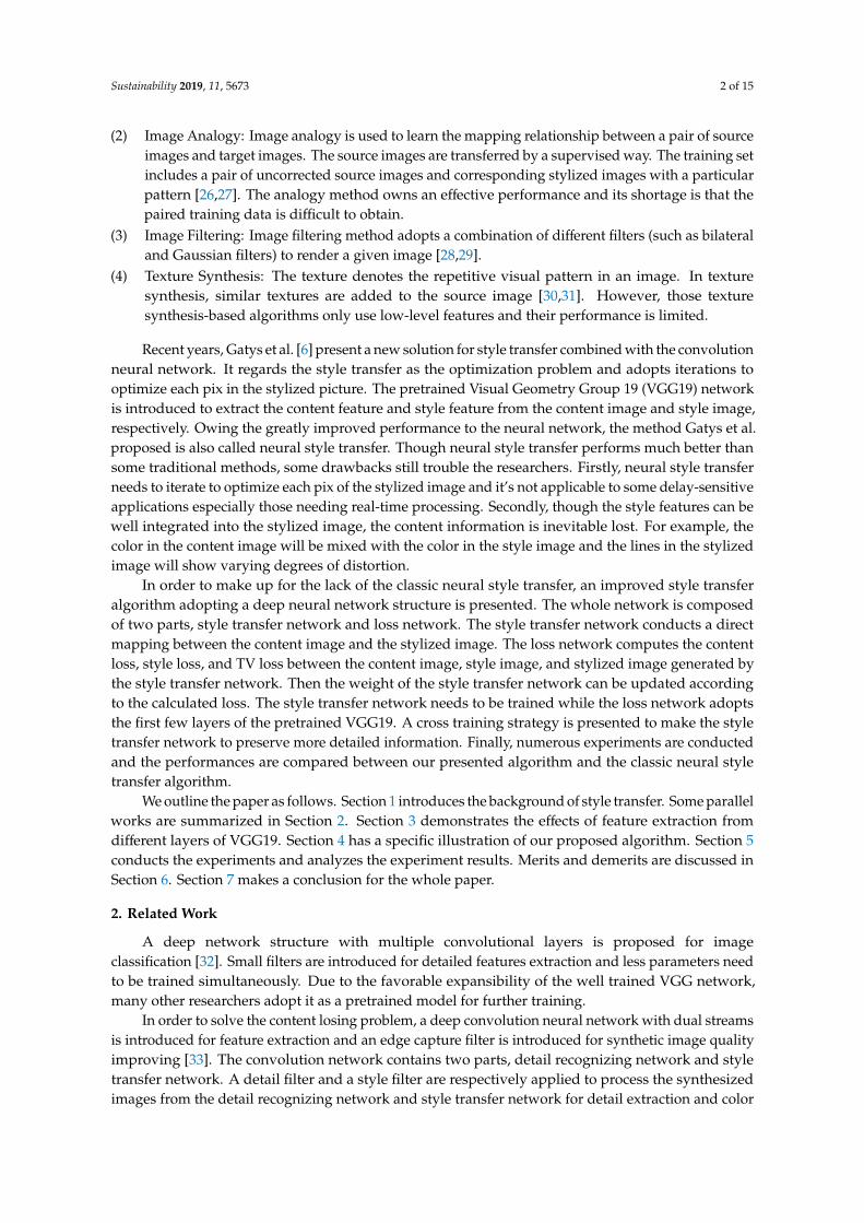
As we can clearly see from Figure 1, the lower layers of VGG19 can preserve much more detailedinformation of content images. While, the deeper layers of VGG19 are more interested in the regulartexture which represents the style of a picture. Therefore, the lower layers of VGG19 are more suitablefor content features extraction and the deeper layers are more suitable for style features extraction.

Sustainability 2019, 11, x FOR PEER REVIEW 4 of 15

ℒ = 1 ( ) − ( ) (3)

We exchange the layers used for features extraction and conduct much experiments. The experiment results are shown as follows.

As we can clearly see from Figure 1, the lower layers of VGG19 can preserve much more detailed information of content images. While, the deeper layers of VGG19 are more interested in the regular texture which represents the style of a picture. Therefore, the lower layers of VGG19 are more suitable for content features extraction and the deeper layers are more suitable for style features extraction.

Figure 1. Feature extraction effects of different of the VGG19.

4. Proposed Method

4.1. Data Processing

We firstly process the input data of the network. In order to avoid the problem of color mixing in the classic neural style transfer, a gray conversion is conducted for the content image. We use the classic physiology formula to transform each RGB pixel of content image into grey pixel as Formula (4). ( ) = ( ) ∙ 0.299 + ( ) ∙ 0.587 + ( ) ∙ 0.144 (4)

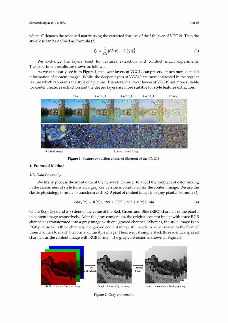
where R(x), G(x), and B(x) denote the value of the Red, Green, and Blue (RBG) channels of the pixel x in content image respectively. After the gray conversion, the original content image with three RGB channels is transformed into a gray image with one grayed channel. Whereas, the style image is an RGB picture with three channels, the grayed content image still needs to be converted to the form of three channels to match the format of the style image. Thus, we just simply stack three identical grayed channels as the content image with RGB format. The gray conversion is shown in Figure 2.

Figure 2. Gray conversion.

Figure 1. Feature extraction effects of different of the VGG19.

4. Proposed Method

4.1. Data Processing

We firstly process the input data of the network. In order to avoid the problem of color mixingin the classic neural style transfer, a gray conversion is conducted for the content image. We use theclassic physiology formula to transform each RGB pixel of content image into grey pixel as Formula (4).

Gray(x) = R(x)·0.299 + G(x)·0.587 + B(x)·0.144 (4)

where R(x), G(x), and B(x) denote the value of the Red, Green, and Blue (RBG) channels of the pixel xin content image respectively. After the gray conversion, the original content image with three RGBchannels is transformed into a gray image with one grayed channel. Whereas, the style image is anRGB picture with three channels, the grayed content image still needs to be converted to the form ofthree channels to match the format of the style image. Thus, we just simply stack three identical grayedchannels as the content image with RGB format. The gray conversion is shown in Figure 2.

Sustainability 2019, 11, x FOR PEER REVIEW 4 of 15

ℒ = 1 ( ) − ( ) (3)

We exchange the layers used for features extraction and conduct much experiments. The experiment results are shown as follows.

As we can clearly see from Figure 1, the lower layers of VGG19 can preserve much more detailed information of content images. While, the deeper layers of VGG19 are more interested in the regular texture which represents the style of a picture. Therefore, the lower layers of VGG19 are more suitable for content features extraction and the deeper layers are more suitable for style features extraction.

Figure 1. Feature extraction effects of different of the VGG19.

4. Proposed Method

4.1. Data Processing

We firstly process the input data of the network. In order to avoid the problem of color mixing in the classic neural style transfer, a gray conversion is conducted for the content image. We use the classic physiology formula to transform each RGB pixel of content image into grey pixel as Formula (4). ( ) = ( ) ∙ 0.299 + ( ) ∙ 0.587 + ( ) ∙ 0.144 (4)

where R(x), G(x), and B(x) denote the value of the Red, Green, and Blue (RBG) channels of the pixel x in content image respectively. After the gray conversion, the original content image with three RGB channels is transformed into a gray image with one grayed channel. Whereas, the style image is an RGB picture with three channels, the grayed content image still needs to be converted to the form of three channels to match the format of the style image. Thus, we just simply stack three identical grayed channels as the content image with RGB format. The gray conversion is shown in Figure 2.

Figure 2. Gray conversion. Figure 2. Gray conversion.

Sustainability 2019, 11, 5673 5 of 15

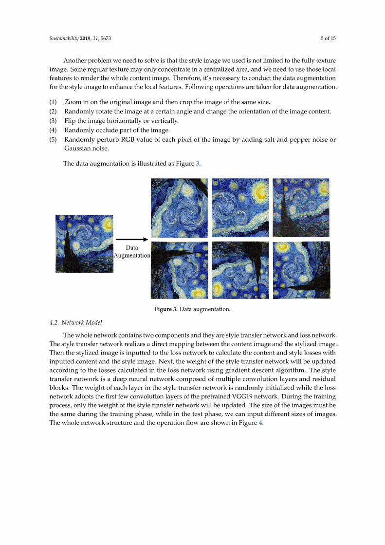
Another problem we need to solve is that the style image we used is not limited to the fully textureimage. Some regular texture may only concentrate in a centralized area, and we need to use those localfeatures to render the whole content image. Therefore, it’s necessary to conduct the data augmentationfor the style image to enhance the local features. Following operations are taken for data augmentation.

(1) Zoom in on the original image and then crop the image of the same size.(2) Randomly rotate the image at a certain angle and change the orientation of the image content.(3) Flip the image horizontally or vertically.(4) Randomly occlude part of the image.(5) Randomly perturb RGB value of each pixel of the image by adding salt and pepper noise or

Gaussian noise.

The data augmentation is illustrated as Figure 3.

Sustainability 2019, 11, x FOR PEER REVIEW 5 of 15

Another problem we need to solve is that the style image we used is not limited to the fully texture image. Some regular texture may only concentrate in a centralized area, and we need to use those local features to render the whole content image. Therefore, it’s necessary to conduct the data augmentation for the style image to enhance the local features. Following operations are taken for data augmentation.

(1) Zoom in on the original image and then crop the image of the same size. (2) Randomly rotate the image at a certain angle and change the orientation of the image content. (3) Flip the image horizontally or vertically. (4) Randomly occlude part of the image. (5) Randomly perturb RGB value of each pixel of the image by adding salt and pepper noise or

Gaussian noise.

The data augmentation is illustrated as Figure 3.

Figure 3. Data augmentation.

4.2. Network Model

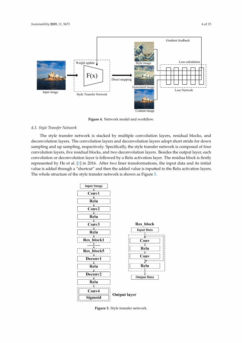
The whole network contains two components and they are style transfer network and loss network. The style transfer network realizes a direct mapping between the content image and the stylized image. Then the stylized image is inputted to the loss network to calculate the content and style losses with inputted content and the style image. Next, the weight of the style transfer network will be updated according to the losses calculated in the loss network using gradient descent algorithm. The style transfer network is a deep neural network composed of multiple convolution layers and residual blocks. The weight of each layer in the style transfer network is randomly initialized while the loss network adopts the first few convolution layers of the pretrained VGG19 network. During the training process, only the weight of the style transfer network will be updated. The size of the images must be the same during the training phase, while in the test phase, we can input different sizes of images. The whole network structure and the operation flow are shown in Figure 4.

Figure 3. Data augmentation.

4.2. Network Model

The whole network contains two components and they are style transfer network and loss network.The style transfer network realizes a direct mapping between the content image and the stylized image.Then the stylized image is inputted to the loss network to calculate the content and style losses withinputted content and the style image. Next, the weight of the style transfer network will be updatedaccording to the losses calculated in the loss network using gradient descent algorithm. The styletransfer network is a deep neural network composed of multiple convolution layers and residualblocks. The weight of each layer in the style transfer network is randomly initialized while the lossnetwork adopts the first few convolution layers of the pretrained VGG19 network. During the trainingprocess, only the weight of the style transfer network will be updated. The size of the images must bethe same during the training phase, while in the test phase, we can input different sizes of images.The whole network structure and the operation flow are shown in Figure 4.

Sustainability 2019, 11, 5673 6 of 15Sustainability 2019, 11, x FOR PEER REVIEW 6 of 15

Figure 4. Network model and workflow.

4.3. Style Transfer Network

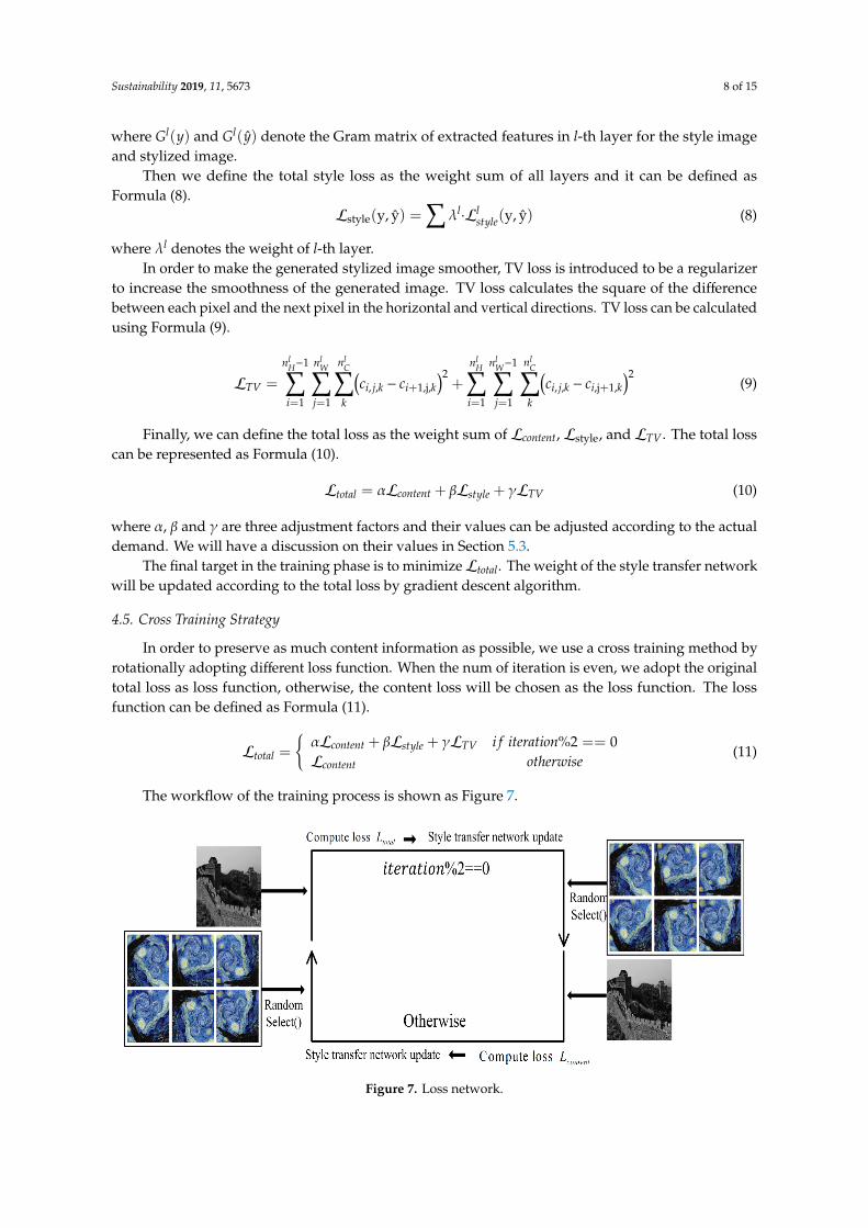
The style transfer network is stacked by multiple convolution layers, residual blocks, and deconvolution layers. The convolution layers and deconvolution layers adopt short stride for down sampling and up sampling, respectively. Specifically, the style transfer network is composed of four convolution layers, five residual blocks, and two deconvolution layers. Besides the output layer, each convolution or deconvolution layer is followed by a Relu activation layer. The residua block is firstly represented by He et al. [40] in 2016. After two liner transformations, the input data and its initial value is added through a “shortcut” and then the added value is inputted to the Relu activation layers. The whole structure of the style transfer network is shown as Figure 5.

Figure 5. Style transfer network.

4.4. Loss Network and Loss Function

Figure 4. Network model and workflow.

4.3. Style Transfer Network

The style transfer network is stacked by multiple convolution layers, residual blocks, anddeconvolution layers. The convolution layers and deconvolution layers adopt short stride for downsampling and up sampling, respectively. Specifically, the style transfer network is composed of fourconvolution layers, five residual blocks, and two deconvolution layers. Besides the output layer, eachconvolution or deconvolution layer is followed by a Relu activation layer. The residua block is firstlyrepresented by He et al. [1] in 2016. After two liner transformations, the input data and its initialvalue is added through a “shortcut” and then the added value is inputted to the Relu activation layers.The whole structure of the style transfer network is shown as Figure 5.

Sustainability 2019, 11, x FOR PEER REVIEW 6 of 15

Figure 4. Network model and workflow.

4.3. Style Transfer Network

The style transfer network is stacked by multiple convolution layers, residual blocks, and deconvolution layers. The convolution layers and deconvolution layers adopt short stride for down sampling and up sampling, respectively. Specifically, the style transfer network is composed of four convolution layers, five residual blocks, and two deconvolution layers. Besides the output layer, each convolution or deconvolution layer is followed by a Relu activation layer. The residua block is firstly represented by He et al. [40] in 2016. After two liner transformations, the input data and its initial value is added through a “shortcut” and then the added value is inputted to the Relu activation layers. The whole structure of the style transfer network is shown as Figure 5.

Figure 5. Style transfer network.

4.4. Loss Network and Loss Function

Figure 5. Style transfer network.

Sustainability 2019, 11, 5673 7 of 15

4.4. Loss Network and Loss Function

The input of the loss network contains three parts, the style image, the stylized image generatedby the style transform network, and the content image. The loss network adopts the first few layers ofthe VGG19 to extract the features of images and its structure and workflow is shown as Figure 6.

Sustainability 2019, 11, x FOR PEER REVIEW 7 of 15

The input of the loss network contains three parts, the style image, the stylized image generated by the style transform network, and the content image. The loss network adopts the first few layers of the VGG19 to extract the features of images and its structure and workflow is shown as Figure 6.

Figure 6. Loss network.

In previous sections, we analyze the ability of feature extraction for different layers in VGG19. The shallower convolutional layers extract the lower features of the image, thus preserving a large amount of detailed information. While the deeper convolution layers can extract higher features in the image, thereby preserving the style information of the image. According to the above rules, we finally adopt “Conv3_1” in VGG19 to extract the content features. Similarly, we adopt “Conv2_1”, “Conv3_1”, “Conv4_1”, and “Conv5_1” in VGG19 to extract the style features.

Content loss describes the difference of features between stylized image and content image. It can be calculated using Formula (5).

ℒ ( , ) = 1∙ ( , , − , , ) (5)

where denotes the batch size of the input data. , , and denotes the height, width, and number of channels of the l-th layer, respectively. , , and , , represent the × -th value of the k-th channel after the content image and stylized image are activated by the l-th layer of VGG19.

Gram matrix can be seen as an eccentric covariance matrix between features of an image. It can reflect the correlation between the two features. Additionally, the diagonal elements of the Gram matrix also reflect the trend of each feature that appears in the image. Gram matrix can measure the features of each dimension and the relationship between different dimensions. Therefore, it can reflect the general style of the entire image. We only need to compare the Gram matrix between different images to represent the difference of their styles. The gram matrix can be calculated using Formula (6).

, ( ) = , , ∙ , , (6)

where and both denote the number of channels in the -th layer. Style loss means the difference between the Gram matrix of the stylized image and the Gram

matrix of the style image. It can be calculated using Formula (7).

ℒ ( , ) = 1 ( , ( ) − , ( )) (7)

Figure 6. Loss network.

In previous sections, we analyze the ability of feature extraction for different layers in VGG19.The shallower convolutional layers extract the lower features of the image, thus preserving a largeamount of detailed information. While the deeper convolution layers can extract higher features inthe image, thereby preserving the style information of the image. According to the above rules, wefinally adopt “Conv3_1” in VGG19 to extract the content features. Similarly, we adopt “Conv2_1”,“Conv3_1”, “Conv4_1”, and “Conv5_1” in VGG19 to extract the style features.

Content loss describes the difference of features between stylized image and content image. It canbe calculated using Formula (5).

Lcontent(y, y) =1

BS·nlHnl

WnlC

nlH∑

i=1

nlW∑

j=1

nlC∑

k=1

(cli, j,k − cl

i, j,k)2

(5)

where BS denotes the batch size of the input data. nlH, nl

W , and nlC denotes the height, width, and

number of channels of the l-th layer, respectively. cli, j,k and cl

i, j,k represent the i× j-th value of the k-thchannel after the content image and stylized image are activated by the l-th layer of VGG19.

Gram matrix can be seen as an eccentric covariance matrix between features of an image. It canreflect the correlation between the two features. Additionally, the diagonal elements of the Grammatrix also reflect the trend of each feature that appears in the image. Gram matrix can measure thefeatures of each dimension and the relationship between different dimensions. Therefore, it can reflectthe general style of the entire image. We only need to compare the Gram matrix between differentimages to represent the difference of their styles. The gram matrix can be calculated using Formula (6).

Glk,k′(y) =

nlH∑

i=1

nlW∑

j=1

cli, j,k·c

li, j,k (6)

where k and k′ both denote the number of channels in the l-th layer.Style loss means the difference between the Gram matrix of the stylized image and the Gram

matrix of the style image. It can be calculated using Formula (7).

Llstyle(y, y) =

1nl

HnlWnl

C

nlC∑

k=1

nlC∑

k′=1

(Glk,k′(y) −Gl

k,k′(y))2

(7)

Sustainability 2019, 11, 5673 8 of 15

where Gl(y) and Gl(y) denote the Gram matrix of extracted features in l-th layer for the style imageand stylized image.

Then we define the total style loss as the weight sum of all layers and it can be defined asFormula (8).

Lstyle(y, y) =∑

λl·L

lstyle(y, y) (8)

where λl denotes the weight of l-th layer.In order to make the generated stylized image smoother, TV loss is introduced to be a regularizer

to increase the smoothness of the generated image. TV loss calculates the square of the differencebetween each pixel and the next pixel in the horizontal and vertical directions. TV loss can be calculatedusing Formula (9).

LTV =

nlH−1∑i=1

nlW∑

j=1

nlC∑k

(ci, j,k − ci+1,j,k

)2+

nlH∑

i=1

nlW−1∑j=1

nlC∑k

(ci, j,k − ci,j+1,k

)2(9)

Finally, we can define the total loss as the weight sum of Lcontent, Lstyle, and LTV. The total losscan be represented as Formula (10).

Ltotal = αLcontent + βLstyle + γLTV (10)

where α, β and γ are three adjustment factors and their values can be adjusted according to the actualdemand. We will have a discussion on their values in Section 5.3.

The final target in the training phase is to minimizeLtotal. The weight of the style transfer networkwill be updated according to the total loss by gradient descent algorithm.

4.5. Cross Training Strategy

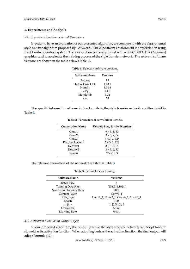
In order to preserve as much content information as possible, we use a cross training method byrotationally adopting different loss function. When the num of iteration is even, we adopt the originaltotal loss as loss function, otherwise, the content loss will be chosen as the loss function. The lossfunction can be defined as Formula (11).

Ltotal =

{αLcontent + βLstyle + γLTV i f iteration%2 == 0Lcontent otherwise

(11)

The workflow of the training process is shown as Figure 7.

Sustainability 2019, 11, x FOR PEER REVIEW 8 of 15

where ( ) and ( ) denote the Gram matrix of extracted features in -th layer for the style image and stylized image.

Then we define the total style loss as the weight sum of all layers and it can be defined as Formula (8). ℒ (y, y) = ∙ ℒ (y, y) (8)

where denotes the weight of -th layer. In order to make the generated stylized image smoother, TV loss is introduced to be a regularizer

to increase the smoothness of the generated image. TV loss calculates the square of the difference between each pixel and the next pixel in the horizontal and vertical directions. TV loss can be calculated using Formula (9).

ℒ = ( , , − , , ) + ( , , − , , ) (9)

Finally, we can define the total loss as the weight sum of ℒ , ℒ , and ℒ . The total loss can be represented as Formula (10). ℒ = ℒ + ℒ + ℒ (10)

where , and are three adjustment factors and their values can be adjusted according to the actual demand. We will have a discussion on their values in Section 5.3.

The final target in the training phase is to minimize ℒ . The weight of the style transfer network will be updated according to the total loss by gradient descent algorithm.

4.5. Cross Training Strategy

In order to preserve as much content information as possible, we use a cross training method by rotationally adopting different loss function. When the num of iteration is even, we adopt the original total loss as loss function, otherwise, the content loss will be chosen as the loss function. The loss function can be defined as Formula (11). ℒ= ℒ + ℒ + ℒ %2 == 0ℒ ℎ (11)

The workflow of the training process is shown as Figure 7.

Figure 7. Loss network.5. Experiments and Analysis.

5.1. Experiment Environment and Parameters

Figure 7. Loss network.

Sustainability 2019, 11, 5673 9 of 15

5. Experiments and Analysis

5.1. Experiment Environment and Parameters

In order to have an evaluation of our presented algorithm, we compare it with the classic neuralstyle transfer algorithm proposed by Gatys et al. The experiment environment is a workstation usingthe Ubuntu operation system. The workstation is also equipped with a GTX 1080 Ti (10G Memory)graphics card to accelerate the training process of the style transfer network. The relevant softwareversions are shown in the table below (Table 1).

Table 1. Relevant software versions.

Software Name Versions

Python 3.7TensorFlow-GPU 1.13.1

NumPy 1.14.6SciPy 1.1.0

Matplotlib 3.02Os 3.7

The specific information of convolution kernels in the style transfer network are illustrated inTable 2.

Table 2. Parameters of convolution kernels.

Convolution Name Kernels Size, Stride, Number

Conv1 9× 9, 1, 32Conv2 3× 3, 2, 64Conv3 3× 3, 2, 128

Res_block_Conv 3× 3, 1, 128Deconv1 3× 3, 2, 64Deconv2 3× 3, 2, 32Conv4 9× 9, 1, 3

The relevant parameters of the network are listed in Table 3.

Table 3. Parameters for training.

Software Name Versions

Batch_Size 4Training Data Size [256,512,1024]

Number of Training Data 5000Content_layer Conv3_1

Style_layer Conv2_1, Conv3_1, Conv4_1, Conv5_1Epoch 100α, β, γ 1, [1,5,10], 1

Optimizer AdamLearning Rate 0.001

5.2. Activation Function in Output Layer

In our proposed algorithm, the output layer of the style transfer network can adopt tanh orsigmoid as its activation function. When adopting tanh as the activation function, the final output willadopt Formula (12).

y = tan h(x) ∗ 122.5 + 122.5 (12)

Sustainability 2019, 11, 5673 10 of 15

where x is the output value of the previous layer. When adopting sigmoid as the activation function,the final output will adopt Formula (13). In both ways, the output value of the output layer can bebetween 0 and 255.

y = sigmoid(x) ∗ 255 (13)

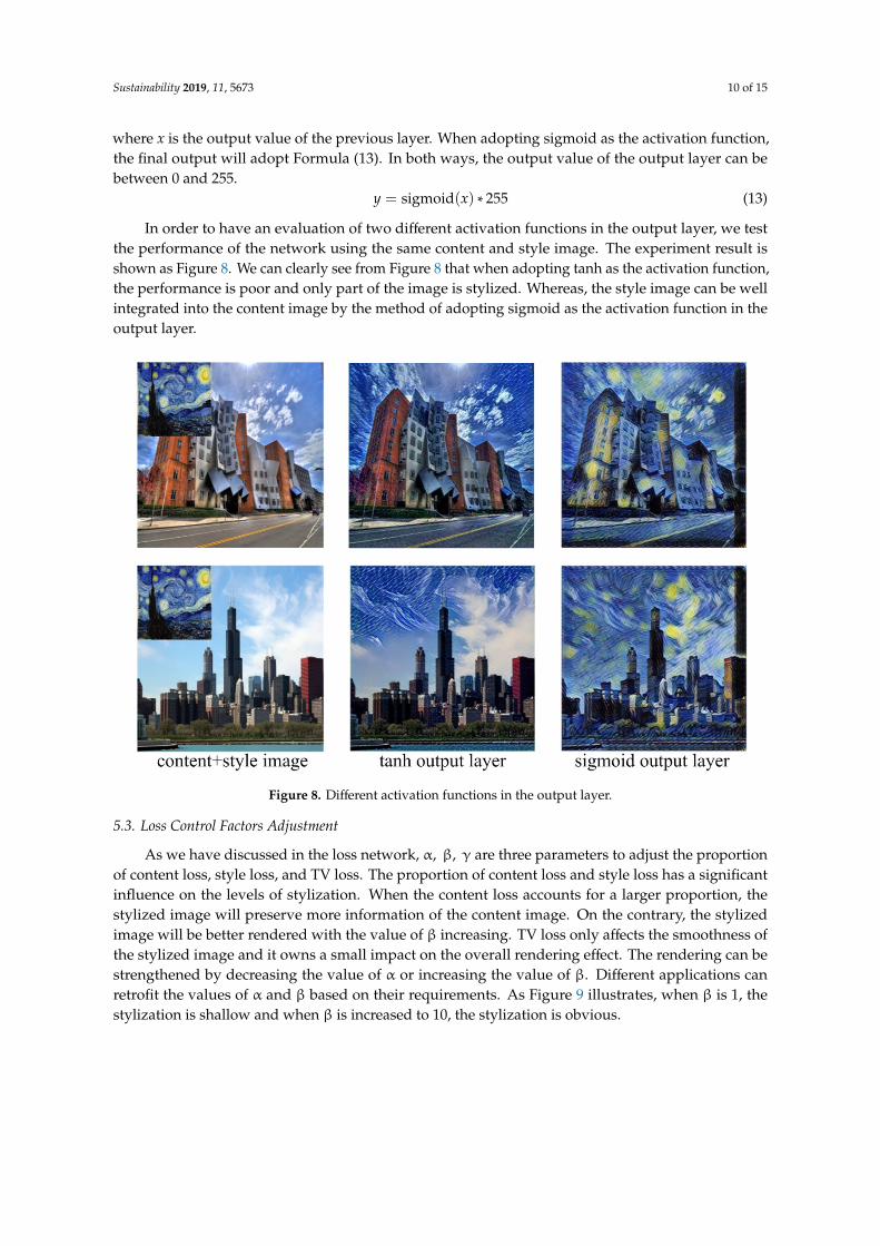
In order to have an evaluation of two different activation functions in the output layer, we testthe performance of the network using the same content and style image. The experiment result isshown as Figure 8. We can clearly see from Figure 8 that when adopting tanh as the activation function,the performance is poor and only part of the image is stylized. Whereas, the style image can be wellintegrated into the content image by the method of adopting sigmoid as the activation function in theoutput layer.

Sustainability 2019, 11, x FOR PEER REVIEW 10 of 15

In order to have an evaluation of two different activation functions in the output layer, we test the performance of the network using the same content and style image. The experiment result is shown as Figure 8. We can clearly see from Figure 8 that when adopting tanh as the activation function, the performance is poor and only part of the image is stylized. Whereas, the style image can be well integrated into the content image by the method of adopting sigmoid as the activation function in the output layer.

Figure 8. Different activation functions in the output layer.

5.3. Loss Control Factors Adjustment

As we have discussed in the loss network, α, β, γ are three parameters to adjust the proportion of content loss, style loss, and TV loss. The proportion of content loss and style loss has a significant influence on the levels of stylization. When the content loss accounts for a larger proportion, the stylized image will preserve more information of the content image. On the contrary, the stylized image will be better rendered with the value of β increasing. TV loss only affects the smoothness of the stylized image and it owns a small impact on the overall rendering effect. The rendering can be strengthened by decreasing the value of α or increasing the value of β. Different applications can retrofit the values of α and β based on their requirements. As Figure 9 illustrates, when β is 1, the stylization is shallow and when β is increased to 10, the stylization is obvious.

Figure 8. Different activation functions in the output layer.

5.3. Loss Control Factors Adjustment

As we have discussed in the loss network, α, β, γ are three parameters to adjust the proportionof content loss, style loss, and TV loss. The proportion of content loss and style loss has a significantinfluence on the levels of stylization. When the content loss accounts for a larger proportion, thestylized image will preserve more information of the content image. On the contrary, the stylizedimage will be better rendered with the value of β increasing. TV loss only affects the smoothness ofthe stylized image and it owns a small impact on the overall rendering effect. The rendering can bestrengthened by decreasing the value of α or increasing the value of β. Different applications canretrofit the values of α and β based on their requirements. As Figure 9 illustrates, when β is 1, thestylization is shallow and when β is increased to 10, the stylization is obvious.

Sustainability 2019, 11, 5673 11 of 15

Sustainability 2019, 11, x FOR PEER REVIEW 11 of 15

Figure 9. Stylized image under different values of β.

5.4. Comparison of Details Preserving

In a stylized image, we expect the objects in it are still recognizable while the background is well rendered. Classic neural style transfer achieves a great performance in image rendering, however, it’s weak to preserve the details in the content image. In order to evaluate the performance of the presented algorithm, we compare it with the classic neural style transfer in terms of details preserving. Both two algorithms adopt the same content and style image with 1024 × 1024 pixels. Classic neural style transfer iterates 1000 times for fully rendering while our presented algorithm iterates 100 epochs for fully training. The experiment result is shown as Figure 10. As Figure 10 illustrates, the classic neural style transfer destroyed partial details from the content image. As you can clearly see in the enlarged picture, that the pillars and the roof of the pavilion have different degrees of missing. While, in our improved algorithm, those details are preserved and the background is well rendered.

Figure 10. Comparison of details preserving.

5.5. Comparison of Characters Rendering

Figure 9. Stylized image under different values of β.

5.4. Comparison of Details Preserving

In a stylized image, we expect the objects in it are still recognizable while the background is wellrendered. Classic neural style transfer achieves a great performance in image rendering, however,it’s weak to preserve the details in the content image. In order to evaluate the performance of thepresented algorithm, we compare it with the classic neural style transfer in terms of details preserving.Both two algorithms adopt the same content and style image with 1024× 1024 pixels. Classic neuralstyle transfer iterates 1000 times for fully rendering while our presented algorithm iterates 100 epochsfor fully training. The experiment result is shown as Figure 10. As Figure 10 illustrates, the classicneural style transfer destroyed partial details from the content image. As you can clearly see in theenlarged picture, that the pillars and the roof of the pavilion have different degrees of missing. While, inour improved algorithm, those details are preserved and the background is well rendered.

Sustainability 2019, 11, x FOR PEER REVIEW 11 of 15

Figure 9. Stylized image under different values of β.

5.4. Comparison of Details Preserving

In a stylized image, we expect the objects in it are still recognizable while the background is well rendered. Classic neural style transfer achieves a great performance in image rendering, however, it’s weak to preserve the details in the content image. In order to evaluate the performance of the presented algorithm, we compare it with the classic neural style transfer in terms of details preserving. Both two algorithms adopt the same content and style image with 1024 × 1024 pixels. Classic neural style transfer iterates 1000 times for fully rendering while our presented algorithm iterates 100 epochs for fully training. The experiment result is shown as Figure 10. As Figure 10 illustrates, the classic neural style transfer destroyed partial details from the content image. As you can clearly see in the enlarged picture, that the pillars and the roof of the pavilion have different degrees of missing. While, in our improved algorithm, those details are preserved and the background is well rendered.

Figure 10. Comparison of details preserving.

5.5. Comparison of Characters Rendering

Figure 10. Comparison of details preserving.

Sustainability 2019, 11, 5673 12 of 15

5.5. Comparison of Characters Rendering

Sometimes, characters are contained in the content image and commonly, we expect thosecharacters can preserve their original features rather than be rendered. In order to have an evaluationof the presented algorithm in terms of characters rendering, we compare it with the classic neuralstyle transfer. Both two algorithms use the same content and style image with 1024 × 1024 pixels.Classic neural style transfer iterates only 500 times to preserve more features of characters and ourpresented algorithm still iterates 100 epochs for fully training. The experiment result is shown asFigure 11. As we can clearly see from Figure 11, that both two algorithms achieve a good performancein stylization. However, the classic neural style transfer algorithm stylizes the characters the same asthe background which results in the facial features, contours, etc., of the characters become blurred anddistorted. This can be explained as that classic neural style transfer adopts the optimization method toconvert the original image to the stylized image. Therefore, the network will treat each pixel in thepicture indiscriminately, making the content image close to the style image. While in our presentedalgorithm, the trained deep neural network will recognize the characters in the image and separatethem from the background. Thus, the characters still keep complete features and clear outlines.

Sustainability 2019, 11, x FOR PEER REVIEW 12 of 15

Sometimes, characters are contained in the content image and commonly, we expect those characters can preserve their original features rather than be rendered. In order to have an evaluation of the presented algorithm in terms of characters rendering, we compare it with the classic neural style transfer. Both two algorithms use the same content and style image with 1024 × 1024 pixels. Classic neural style transfer iterates only 500 times to preserve more features of characters and our presented algorithm still iterates 100 epochs for fully training. The experiment result is shown as Figure 11. As we can clearly see from Figure 11, that both two algorithms achieve a good performance in stylization. However, the classic neural style transfer algorithm stylizes the characters the same as the background which results in the facial features, contours, etc., of the characters become blurred and distorted. This can be explained as that classic neural style transfer adopts the optimization method to convert the original image to the stylized image. Therefore, the network will treat each pixel in the picture indiscriminately, making the content image close to the style image. While in our presented algorithm, the trained deep neural network will recognize the characters in the image and separate them from the background. Thus, the characters still keep complete features and clear outlines.

Figure 11. Comparison of characters rendering.

5.6. Comparison of Time Consuming

Finally, we have an evaluation of our presented algorithm compared with the classic neural style transfer in terms of time consuming. Images with different pixels are tested respectively. Both in the classic neural style transfer and our present algorithm, the network needs to be adjusted to fit different sizes of input data. Graphics Processing Unit (GPU) is only used when execute the two different algorithms. Images with high resolution will have a better visual effect and meanwhile, it takes more time for the network to render. Experiment result is shown in Table 4. As we can clearly see from Table 4, the time consuming of both two algorithms increases with image pixel increasing. For the image with the same pixel, our proposed algorithm achieves an enhancement of three orders of magnitude compared with the classic neural style transfer. However, in our presented algorithm, a long time is needed to train the style transfer network.

Table 4. Comparison of time consuming of different algorithms.

Algorithm Classic Neural Style Transfer Algorithm Ours

Image Size 100 Iterations 500 Iterations 1000 Iterations

Training Time 1 Iteration

256 × 256 5.4 s 26.1 s 51.3 s 5 h 32 m 0.05 s 512 × 512 15.1 s 69.6 s 122.7 s 8 h 47 m 0.1 s

1024 × 1024 30.5 s 138.6 s 240.1 s 12 h 17 m 0.2 s

Figure 11. Comparison of characters rendering.

5.6. Comparison of Time Consuming

Finally, we have an evaluation of our presented algorithm compared with the classic neural styletransfer in terms of time consuming. Images with different pixels are tested respectively. Both inthe classic neural style transfer and our present algorithm, the network needs to be adjusted to fitdifferent sizes of input data. Graphics Processing Unit (GPU) is only used when execute the twodifferent algorithms. Images with high resolution will have a better visual effect and meanwhile, ittakes more time for the network to render. Experiment result is shown in Table 4. As we can clearlysee from Table 4, the time consuming of both two algorithms increases with image pixel increasing.For the image with the same pixel, our proposed algorithm achieves an enhancement of three orders ofmagnitude compared with the classic neural style transfer. However, in our presented algorithm, along time is needed to train the style transfer network.

Table 4. Comparison of time consuming of different algorithms.

Algorithm Classic Neural Style Transfer Algorithm Ours

Image Size 100 Iterations 500 Iterations 1000 Iterations Training Time 1 Iteration

256 × 256 5.4 s 26.1 s 51.3 s 5 h 32 m 0.05 s512 × 512 15.1 s 69.6 s 122.7 s 8 h 47 m 0.1 s

1024 × 1024 30.5 s 138.6 s 240.1 s 12 h 17 m 0.2 s

Sustainability 2019, 11, 5673 13 of 15

5.7. Other Examples Using Proposed Algorithm

Some other examples using the proposed algorithm are shown as Figure 12.Sustainability 2019, 11, x FOR PEER REVIEW 13 of 15

Figure 12. Examples using proposed algorithm.

6. Discussion

The convolution neural network owns an excellent ability for features extraction and it provides

an alternative way for the feature comparison between different images. The classic neural style

transfer algorithm regards the stylization task as an image-optimization-based online processing

problem. While, our presented algorithm regards it as a model-optimization-based offline processing

problem. The most prominent advantage of the presented algorithm is the short running time for

stylization. Since the network model can be trained in advance, it’s suitable for those delay sensitive

application especially real-time style transfer. Another advantage is that it can separate important

targets from the background to avoid the content loss. Contrary to image-optimization, model-

optimization aims to train a model to directly map the content image to the stylized image. The

training process makes the model capable to recognize different objects such as characters and

buildings, therefore, it can better preserve the details of those objects and separate them from the

background.

Meanwhile, there are also some demerits of the proposed algorithm. It’s inflexible to switch the

style. Once we want to change the style, we need to train a brand-new model which may take a lot of

time. However, the image-optimization-based method only needs to change the style image and then

iterates to the final solution. Additionally, our presented algorithm needs to run on the device with

better performance such as computation and memory which increases the cost.

7. Conclusion

Classic neural style transfer has the demerits of time consuming and details losing. In order to

accelerate the speed of stylization and improve the quality of the stylized image, in this paper, we

present an improved style transfer algorithm based on a deep feedforward neural network. A style

transfer network stacked by multiple convolution layers and a loss network work based on VGG19

are respectively constructed. Three different losses which represent the content, style, and

smoothness are defined in the loss network. Then, the style transfer network is trained in advance,

adopting the training set, and the loss is calculated by the loss network to update the weight of the

style transfer network. Meanwhile, a cross training strategy is adopted during the training process.

Our feature work will mainly focus on single model based multi-style transfer and special style

transfer combined with Generative Adversarial Networks (GAN).

Author Contributions: Z.G. conceived and designed the experiments; C.Z. and Y.G. performed the experiments

and analyzed the data. J.W. wrote this paper.

Figure 12. Examples using proposed algorithm.

6. Discussion

The convolution neural network owns an excellent ability for features extraction and it provides analternative way for the feature comparison between different images. The classic neural style transferalgorithm regards the stylization task as an image-optimization-based online processing problem.While, our presented algorithm regards it as a model-optimization-based offline processing problem.The most prominent advantage of the presented algorithm is the short running time for stylization.Since the network model can be trained in advance, it’s suitable for those delay sensitive applicationespecially real-time style transfer. Another advantage is that it can separate important targets from thebackground to avoid the content loss. Contrary to image-optimization, model-optimization aims totrain a model to directly map the content image to the stylized image. The training process makes themodel capable to recognize different objects such as characters and buildings, therefore, it can betterpreserve the details of those objects and separate them from the background.

Meanwhile, there are also some demerits of the proposed algorithm. It’s inflexible to switch thestyle. Once we want to change the style, we need to train a brand-new model which may take a lot oftime. However, the image-optimization-based method only needs to change the style image and theniterates to the final solution. Additionally, our presented algorithm needs to run on the device withbetter performance such as computation and memory which increases the cost.

7. Conclusions

Classic neural style transfer has the demerits of time consuming and details losing. In orderto accelerate the speed of stylization and improve the quality of the stylized image, in this paper,we present an improved style transfer algorithm based on a deep feedforward neural network. A styletransfer network stacked by multiple convolution layers and a loss network work based on VGG19 arerespectively constructed. Three different losses which represent the content, style, and smoothnessare defined in the loss network. Then, the style transfer network is trained in advance, adopting thetraining set, and the loss is calculated by the loss network to update the weight of the style transfernetwork. Meanwhile, a cross training strategy is adopted during the training process. Our feature

Sustainability 2019, 11, 5673 14 of 15

work will mainly focus on single model based multi-style transfer and special style transfer combinedwith Generative Adversarial Networks (GAN).

Author Contributions: Z.G. conceived and designed the experiments; C.Z. and Y.G. performed the experimentsand analyzed the data. J.W. wrote this paper.

Acknowledgments: The authors are thankful to the editor and reviewers for their hard work which largelyimprove the quality of this paper.

Conflicts of Interest: The authors declare no conflict of interest.

Data Availability: The data that support the findings of this study are available from the corresponding authorupon reasonable request.

References

1. He, K.; Zhang, X.; Ren, S.; Sun, J. Deep residual learning for image recognition. arXiv 2015, arXiv:1512.03385.2. Zou, W.; Li, X.; Li, S. Chinese painting rendering by adaptive style transfer. In Pattern Recognition and

Computer Vision; Springer: Cham, Switzerland, 2018; pp. 3–14. [CrossRef]3. Zheng, C.; Zhang, Y. Two-stage color ink painting style transfer via convolution neural network.

In Proceedings of the 2018 15th International Symposium on Pervasive Systems, Algorithms and Networks(I-SPAN), Yichang, China, 16–18 October 2018. [CrossRef]

4. Liu, S.; Guo, C.; Sheridan, J.T. A review of optical image encryption techniques. Opt. Laser Technol. 2014, 57,327–342. [CrossRef]

5. Wu, C.; Ko, J.; Davis, C.C. Imaging through strong turbulence with a light field approach. Opt. Express. 2016,24, 11975–11986. [CrossRef] [PubMed]

6. Gatys, L.A.; Ecker, A.S.; Bethge, M. A Neural algorithm of artistic style. arXiv 2015, arXiv:1508.06576.[CrossRef]

7. Karen, S.; Andrew, Z. Very deep convolutional networks for large-scale image recognition. arXiv 2015,arXiv:1409.1556.

8. Wang, J.; Gao, Y.; Liu, W.; Sangaiah, A.K.; Kim, H.J. An intelligent data gathering schema with data fusionsupported for mobile sink in wireless sensor networks. Int. J. Distrib. Sens. Netw. 2019, 15. [CrossRef]

9. Qiu, H.; Huang, X. An Improved image transformation network for neural style transfer. In Proceedingsof the 2nd International Conference on Intelligence Science (ICIS), Shanghai, China, 25–28 October 2017.[CrossRef]

10. Wang, J.; Gu, X.; Liu, W.; Sangaiah, A.K.; Kim, H. An empower hamilton loop based data collection algorithmwith mobile agent for WSNs. Hum.-Cent. Comput. Inf. Sci. 2019, 9, 18. [CrossRef]

11. Zeng, H.; Liu, Y.; Li, S.; Che, J.; Wang, X. Convolutional neural network based multi-feature fusion fornon-rigid 3D model retrieval. J. Inf. Process. Syst. 2018, 14, 176–190.

12. Daru, P.; Gada, S.; Chheda, M.; Raut, P. Neural style transfer to design drapes. arXiv 2017, arXiv:1707.09899.13. Pan, J.S.; Kong, L.P.; Sung, T.W.; Tsai, P.W.; Snasel, V. Alpha-fraction first strategy for hierarchical wireless

sensor networks. J. Internet Technol. 2018, 19, 1717–1726.14. Johnson, J.; Alahi, A.; Li, F.-F. Perceptual losses for real-time style transfer and super-resolution. arXiv 2016,

arXiv:1603.08155.15. Qiu, X.; Jia, W.; Li, H. A font style learning and transferring method based on strokes and structure of Chinese

characters. In Proceedings of the 2012 International Conference on Computer Science and Service System,Nanjing, China, 11–13 August 2012; pp. 1836–1839. [CrossRef]

16. Pan, J.S.; Lee, C.Y.; Sghaier, A.; Zeghid, M.; Xie, J.F. Novel systolization of subquadratic space complexitymultipliers based on toeplitz matrix–vector product approach. IEEE Trans. Very Large Scale Integr. 2019, 27,1614–1622. [CrossRef]

17. Azadi, S.; Fisher, M.; Kim, V.G.; Wang, Z.; Shechtman, E.; Darrell, T. Multi-content gan for few-shot font styletransfer. arXiv 2018, arXiv:1712.00516.

18. Wang, J.; Gao, Y.; Liu, W.; Sangaiah, A.K.; Kim, H.J. Energy efficient routing algorithm with mobile sinksupport for wireless sensor networks. Sensors 2019, 19, 1494. [CrossRef] [PubMed]

19. Nguyen, T.T.; Pan, J.S.; Dao, T.K. An improved flower pollination algorithm for optimizing layouts of nodesin wireless sensor network. IEEE Access 2019, 7, 75985–75998. [CrossRef]

Sustainability 2019, 11, 5673 15 of 15

20. Meng, Z.Y.; Pan, J.S.; Tseng, K.K. PaDE: An enhanced differential evolution algorithm with novel controlparameter adaptstion schemes for numerical optimization. Knowl.-Based Syst. 2019, 168, 80–99. [CrossRef]

21. Pan, J.S.; Kong, L.P.; Sung, T.W.; Tsai, P.W.; Snasel, V. A clustering scheme for wireless sensor networks basedon genetic algorithm and dominating Set. J. Internet Technol. 2018, 19, 1111–1118.

22. Wu, T.Y.; Chen, C.M.; Wang, K.H.; Meng, C.; Wang, E.K. A provably secure certificateless public keyencryption with keyword search. J. Chin. Inst. Eng. 2019, 42, 20–28. [CrossRef]

23. Liu, J.; Yang, W.; Sun, X.; Zeng, W. Photo stylistic brush: Robust style transfer via superpixel-based bipartitegraph. IEEE Trans. Multimed. 2017, 20, 1724–1737. [CrossRef]

24. Wang, J.; Gao, Y.; Wang, K.; Sangaiah, A.K.; Lim, S.J. An affinity propagation-based self-adaptive clusteringmethod for wireless sensor networks. Sensors 2019, 19, 2579. [CrossRef]

25. Wang, J.; Gao, Y.; Yin, X.; Li, F.; Kim, H.J. An enhanced PEGASIS algorithm with mobile sink support forwireless sensor networks. Wirel. Commun. Mob. Comput. 2018, 2018, 9472075. [CrossRef]

26. Ghrabat, M.J.J.; Ma, G.; Maolood, I.Y.; Alresheedi, S.S.; Abduljabbar, Z.A. An effective image retrieval basedon optimized genetic algorithm utilized a novel SVM-based convolutional neural network classifier. Hum.-Cent. Comput. Inf. Sci. 2019, 9, 31. [CrossRef]

27. Zeng, D.; Dai, Y.; Li, F.; Wang, J.; Sangaiah, A.K. Aspect based sentiment analysis by a linguisticallyregularized CNN with gated mechanism. J. Intell. Fuzzy Syst. 2019, 36, 3971–3980. [CrossRef]

28. Zhang, L.; Wang, Y. Stable and refned style transfer using zigzag learning algorithm. Neural Process. Lett.2019. [CrossRef]

29. Tu, Y.; Lin, Y.; Wang, J.; Kim, J.U. Semi-supervised learning with generative adversarial networks on digitalsignal modulation classification. Comput. Mater. Contin. 2018, 55, 243–254.

30. Li, C.; Liang, M.; Song, W.; Xiao, K. A multi-scale parallel convolutional neural network based intelligenthuman identification using face information. J. Inf. Process. Syst. 2018, 14, 1494–1507.

31. Liu, D.; Yu, W.; Yao, H. Style transfer with content preservation from multiple images. In Advances inMultimedia Information Processing—PCM 2017; Springer: Cham, Switzerland, 2017. [CrossRef]

32. Hu, J.; He, K.; Hopcroft, J.E.; Zhang, Y. Deep compression on convolutional neural network for artistic styletransfer. In Theoretical Computer Science; Springer: Singapore, 2017. [CrossRef]

33. Wang, L.; Wang, Z.; Yang, X.; Hu, S.; Zhang, J. Photographic style transfer. Vis. Comput. 2018. [CrossRef]34. Zhang, W.; Li, G.; Ma, H.; Yu, Y. Automatic color sketch generation using deep style transfer. IEEE Comput.

Graph. Appl. 2019, 39, 26–37. [CrossRef]35. Zhao, H.H.; Rosin, P.L.; Lai, Y.K.; Lin, M.G.; Liu, Q.Y. Image neural style transfer with global and local

optimization fusion. IEEE Access 2019, 7, 85573–85580. [CrossRef]36. Yoon, Y.B.; Kim, M.S.; Choi, H.C. End-to-end learning for arbitrary image style transfer. Electron. Lett. 2018,

54, 1276–1278. [CrossRef]37. Liu, Y.; Xu, Z.; Ye, W.; Zhang, Z.; Weng, S.; Chang, C.C.; Tang, H. Image neural style transfer with preserving

the salient regions. IEEE Access 2019, 7, 40027–40037. [CrossRef]38. Chen, Y.; Lai, Y.; Liu, Y. CartoonGAN: Generative adversarial networks for photo cartoonization.

In Proceedings of the 2018 IEEE/CVF Conference on Computer Vision and Pattern Recognition, Salt Lake City,UT, USA, 18–23 June 2018. [CrossRef]

39. Chen, X.; Xu, C.; Yang, X.; Song, L.; Tao, D. Gated-gan: Adversarial gated networks for multi-collection styletransfer. IEEE Trans. Image Process. 2018, 28, 546–560. [CrossRef] [PubMed]

© 2019 by the authors. Licensee MDPI, Basel, Switzerland. This article is an open accessarticle distributed under the terms and conditions of the Creative Commons Attribution(CC BY) license (http://creativecommons.org/licenses/by/4.0/).