Second order models and traffic data from mobile sensors

Transportation Research Part C 52 (2015) 32–56

Contents lists available at ScienceDirect

Transportation Research Part C

journal homepage: www.elsevier .com/locate / t rc

Second-order models and traffic data from mobile sensors

http://dx.doi.org/10.1016/j.trc.2014.12.0130968-090X/� 2015 Elsevier Ltd. All rights reserved.

⇑ Corresponding author.E-mail addresses: [email protected] (B. Piccoli), [email protected] (K. Han), [email protected] (T.L. Friesz), [email protected]

[email protected] (J. Tang).

Benedetto Piccoli a, Ke Han b,⇑, Terry L. Friesz c, Tao Yao c, Junqing Tang b

a Department of Mathematics, Rutgers University, Camden, NJ 08102, USAb Department of Civil and Environmental Engineering, Imperial College London, London SW7 2BU, UKc Department of Industrial and Manufacturing Engineering, Pennsylvania State University, University Park, PA 16802, USA

a r t i c l e i n f o a b s t r a c t

Article history:Received 24 August 2013Received in revised form 28 December 2014Accepted 28 December 2014

Keywords:Mobile sensingPhase transition modelHigher-order traffic quantityEmission rate

Mobile sensing enabled by GPS or smart phones has become an increasingly importantsource of traffic data. For sufficient coverage of the traffic stream, it is important to main-tain a reasonable penetration rate of probe vehicles. From the standpoint of capturinghigher-order traffic quantities such as acceleration/deceleration, emission and fuelconsumption rates, it is desirable to examine the impact on the estimation accuracy ofsampling frequency on vehicle position. Of the two issues raised above, the latter is rarelystudied in the literature. This paper addresses the impact of both sampling frequency andpenetration rate on mobile sensing of highway traffic. To capture inhomogeneous drivingconditions and deviation of traffic from the equilibrium state, we employ the second-orderphase transition model (PTM). Several data fusion schemes that incorporate vehicle trajec-tory data into the PTM are proposed. And, a case study of the NGSIM dataset is presentedwhich shows the estimation results of various Eulerian and Lagrangian traffic quantities.The findings show that while first-order traffic quantities can be accurately estimated evenwith a low sampling frequency, higher-order traffic quantities, such as acceleration, devi-ation, and emission rate, tend to be misinterpreted due to insufficiently sampled vehiclelocations. We also show that a correction factor approach has the potential to reduce thesensing error arising from low sampling frequency and penetration rate, making the esti-mation of higher-order quantities more robust against insufficient data coverage of thehighway traffic.

� 2015 Elsevier Ltd. All rights reserved.

1. Introduction

With the increased availability of mobile traffic data and the advancement of sensing technology, data collected throughGPS, smart phones or other mobile devices have become a major source of traffic information for various applications.Advantages of mobile sensing, in comparison with fixed-location sensing (e.g. using loop detectors and cameras), includepotentially complete spatial and temporal coverage of traffic network and high positioning accuracy (Herrera et al., 2010).

Traffic data related to speed, density, queue size and travel time, which are categorized as lower-order quantities, canoften be estimated in conjunction with first-order traffic flow models such as the Lighthill–Whitham–Richards (LWR) model(Lighthill and Whitham, 1955; Richards, 1956) and the cell transmission model (CTM) (Daganzo, 1994). Strub and Bayen(2006) employ a weak formulation of boundary conditions for the LWR model based on the Godunov scheme, which is then

(T. Yao),

http://crossmark.crossref.org/dialog/?doi=10.1016/j.trc.2014.12.013&domain=pdf

http://dx.doi.org/10.1016/j.trc.2014.12.013

mailto:[email protected]





http://dx.doi.org/10.1016/j.trc.2014.12.013

http://www.sciencedirect.com/science/journal/0968090X

http://www.elsevier.com/locate/trc

B. Piccoli et al. / Transportation Research Part C 52 (2015) 32–56 33

applied to the I-80 highway dataset. In Christiani et al. (2010), the LWR model is discretized in connection with initial andboundary conditions, which is applied to traffic estimation on a circular urban motorway using mobile data. Claudel andBayen (2011) propose convex formulations for data assimilation using both Eulerian (fixed) and Lagrangian (mobile) trafficdata based on the Hamilton–Jacobi representation of highway traffic and the generalized Lax–Hopf formula. Work et al.(2010) employ a velocity-based LWR model with transformed fundamental diagram to perform data fusion using ensembleKalman filter. Independently, Yuan et al. (2011) consider the LWR model with a transformed coordinate system, namely theLagrangian coordinates, and perform traffic estimation using extended Kalman filter. These studies mainly focus on freewaytraffic.

In another line of research, mobile data have been used extensively for estimating queue size and delay at signalizedintersections in arterial networks. Ban et al. (2009) use sampled vehicle travel times to estimate delay patterns near a sig-nalized junction, where the authors use the LWR theory with a triangular fundamental diagram to express the relationshipamong flow, shock speed, queue size and queuing time. Following this work, Ban et al. (2011) devise a reverse modeling pro-cess that construct the dynamic queue length in real time. Cheng et al. (2012) further explore probe vehicle trajectories inestimating queue size in real time with the benefit of less communication cost in data collection. Comert and Cetin (2009)propose a statistical approach for estimating queue length using an analytical formulation based on conditional probabilities.The authors also address the estimation accuracy with a wide range of probe penetration rates. Argote et al. (2011) considerseveral measures of effectiveness and estimation methods to identify proper penetration rates.

Although the LWR model and the CTM have been used effectively in estimating lower-order quantities, they have beenused less frequently in estimating higher-order traffic quantities such as acceleration/deceleration, deviation (perturbation),emission and fuel consumption rates. There exist a number of attempts to estimate acceleration/deceleration or emissionrates through differentiating macroscopic traffic quantities analytically or numerically (e.g. Luspay et al., 2010). However,in this process higher-order variations inherent in these quantities, typically on a microscopic scale, are insufficientlycaptured due to the low temporal-spatial resolution of the traffic data and the discrete models. To fill this gap, this paperproposes a second-order traffic flow model supported by high-resolution mobile data to address the issue of estimatinghigh-order traffic quantities. Unlike most existing studies on mobile sensing which primarily focus on probe penetration rate(Demers et al., 2006; Kwon et al., 2007; Yim and Cayford, 2001), we consider the additional effect of under sampling on theestimation accuracy. This is a concern because most mobile data provide location or speed of a moving vehicle every 3-4 s(such as GPS data), but higher-order variations in speed, acceleration and emission may take place on a smaller time scale;this is true especially for congested and unstable traffic. Such an observation has urged the need to examine the efficacy ofexisting sensing technologies and estimation methods in reconstructing the profiles for these higher-order quantities.

The second-order traffic flow model employed by this paper is the hyperbolic phase transition model (PTM), first intro-duced by Colombo (2002) and studied subsequently by Colombo and Corli (2002), Colombo et al. (2007) and Blandinet al. (2012). Second- and higher-order traffic models were proposed by many researchers to overcome some limitationsof the LWR model in describing complex waves observed in vehicular traffic. Most second-order models tend to pose, inaddition to the LWR-type equation for the conservation of vehicles, a second equation for the conservation or balance ofmomentum. One of the first such models is by Payne and Whitham in the 1970s (Payne, 1971; Whitham, 1974). In a cele-brated paper (Daganzo, 1995) Daganzo criticized second-order models by showing various drawbacks including the possi-bility of cars going backward. Most of such drawbacks were later addressed by the Aw–Rascle–Zhang model, independentlyproposed by Aw and Rascle (2000) and Zhang (2002). More recently, the phase transition models drew increased attentionfrom researchers for their capability of representing complex waves while keeping the LWR structure for light traffic, seeBlandin et al. (2011) for more detailed discussion.

Let us further comment on the possible use of second-order model for urban arterial traffic. The aforementioned complexwave phenomenon, well captured by second-order models, are mainly observed in highway traffic. Indeed, phantom waves,stop-and-go waves and others need a long stretch of road with no interruption to manifest themselves. The situation of arte-rial traffic is quite different because of the presence of many junctions with traffic signs or signals. Since the LWR model cap-tures well backward wave propagation from junctions or signals, and vehicle movements on arterials are relatively uniform,it is typically sufficient to describe arterial traffic, while very limited to model more complex waves in highway traffic.

In order to address issues related to higher-order traffic quantities, we focus on the Next Generation SIMulation (NGSIM)dataset.1 The NGSIM program collected high-quality traffic and vehicle trajectory data on a stretch of I-80 highway in California.A total of 45 min of traffic data were collected, segmented into three 15 min periods. The dataset contains vehicle trajectoryrecorded at a high resolution of every 0.1 s. Derived information on instantaneous velocity and acceleration is also available.A detailed description of the NGSIM field experiment and data will be provided in Section 5.

1.1. Contribution and findings

This paper addresses the effectiveness of mobile sensing and traffic estimation taking into account two main factors:sampling frequency and probe penetration rate. The subject of estimation will include both lower- and higher-order trafficquantities. To support this study, we employ the second-order phase transition model (PTM) as well as its modifications. The

1 http://ngsim-community.org/.

http://ngsim-community.org/

34 B. Piccoli et al. / Transportation Research Part C 52 (2015) 32–56

underpinning dataset is provided by the NGSIM program, which contains high resolution vehicle trajectories on a segment ofI-80. Such detailed vehicle trajectories provide unique information regarding the higher-order variations of traffic, which isunavailable through traditional mobile or fixed sensors. We propose several data fusion schemes that integrate mobile datainto the PTM under various assumptions. As a result, vehicle speed, acceleration, density, deviation (perturbation), enginepower demand and emission rate can be estimated along vehicle trajectories (these quantities are Lagrangian as they areassociated with moving vehicles). We demonstrate how these estimations deteriorate with less frequent sampling of vehiclelocations, with special attention given to the difference between lower- and higher-order quantities. We also present amethod for estimating Eulerian traffic quantities; i.e. quantities associated with a give point in the temporal-spatial domain.The joint effects of sampling frequency and probe penetration rate in reconstructing lower- and higher-order quantities areassessed. It is found that, for both Lagrangian and Eulerian estimations, lower-order traffic variables (such as density) can beestimated relatively accurately, while higher-order ones (such as emission and perturbation) are far more susceptible tounder sampling and lower penetration rate. This is consistent with the expectation that higher-order variations tend tobe overlooked by data presented at a low resolution. We also show that Eulerian estimation of higher-order quantities enjoyimproved accuracy than Lagrangian estimation due to the effect of spatial–temporal aggregation. And, the efficacy ofEulerian estimation can be further improved by applying a correction factor approach. This is demonstrated by using hydro-carbon emission rate as an example and proven to be an effective estimation method even with low sampling frequency andpenetration rate.

The main contributions and findings made by this paper are summarized as follows:

� Several methods for integrating vehicle trajectory data into the phase transition model are proposed. These methods arefurther extended to perform both Lagrangian and Eulerian estimation of traffic quantities.� Along each vehicle trajectory, the estimation of higher-order traffic quantities deteriorates significantly when the sam-

pling frequency decreases, while the estimation of first-order quantities remain relatively accurate with the same sam-pling frequency.� For the Eulerian estimation, we provide numerical results on density (first-order) and HC emission rate (higher-order)

with varying sampling frequency and penetration rate. The HC estimation enjoys an improved accuracy compared tothe Lagrangian estimation due to the averaging of multiple measurements, although it also deteriorates with under sam-pling and lower penetration rate.� We provide a comparative study of the LWR model (first order) and the phase transition model in terms of estimating

first-order density (notice that higher-order quantities such as acceleration and perturbation are not captured explicitlyby the LWR model). The PTM outperforms the LWR model in terms of estimation accuracy. In addition, deviation of indi-vidual vehicles from the equilibrium state, which is not captured by the LWR model, has been illustrated numerically.� A correction factor approach is proposed for estimating HC emission rate with insufficient mobile data coverage. We

employ a regression model to correct the predicted emission rate in order to minimize the misinterpretation of theground truth caused by lower sampling frequencies or probe penetration rates. The validity and effectiveness of thisapproach is shown through cross validation.

The rest of this paper is organized as follows: Section 2 recaps several numerical approximations of basic traffic quantitiesbased on vehicle trajectory data. Section 3 introduces the phase transition model (PTM), followed by three data fusionschemes. Models for HC emission rate and engine power demand are also described. Section 4 illustrates the procedureemployed to reduce random noises in the raw dataset and errors derived from numerical differentiation. In Section 5, wecalibrate the PTM using the NGSIM data. Section 6 assesses the estimation quality for first- and second-order quantitiesalong vehicle trajectories, when the sampling frequency varies. Sections 7 and 8 perform Eulerian estimation for densityand HC emission rate respectively, and evaluate its effectiveness against various sampling frequencies and penetration rates.A correction factor approach for improving the accuracy and reliability of HC emission is also presented and tested. Section 9provides some concluding remarks.

2. Estimating basic traffic quantities

Onboard sensors such as GPS and smart phone measure the location of a moving car every dt seconds, where dt is relatedto the device’s characteristics such as desired precision and transmission capacity. For a given vehicle, we denote by xðtÞ itslocation and by vðtÞ its velocity at time t. Assume that the location is recorded at three consecutive time stamps t1; t2 and t3

with t2 � t1 ¼ t3 � t2 ¼ dt. From these measurements one can deduce approximate velocities in the time intervals ½t1; t2� and½t2; t3� respectively as

v1;2 ¼xðt2Þ � xðt1Þ

dt; v2;3 ¼

xðt3Þ � xðt2Þdt

ð2:1Þ

The velocity at time t2 is approximated as

vðt2Þ �v1;2 þ v2;3

2¼ xðt3Þ � xðt1Þ

2dtð2:2Þ


One also gets estimate for the acceleration:

aðt2Þ ¼DDt

vðt; xÞ��t¼t2

� v2;3 � v1;2

dt¼ xðt3Þ � 2xðt2Þ þ xðt1Þ

dt2 ð2:3Þ

where vðt; xÞ denotes the velocity function in the Eulerian coordinates; D=Dt ¼ d=dt þ v � d=dx represents the material deriv-ative in the Eulerian coordinates corresponding to the acceleration of the car in the Lagrangian coordinate.

Another important quantity to estimate is the spatial variation of velocity in the Eulerian coordinate. For notation con-venience, we set xi ¼

: xðtiÞ. Assuming a mild variation in time of the Eulerian velocity vðt; xÞ, we write:

v t2;x2 þ x1

2

� �� v1;2; v t2;

x3 þ x2

2

� �� v2;3;

from which we get, by setting dx ¼ x3þx22 � x2þx1

2 , that

@

@xv t2;

x3þx22 þ x2þx1

2

2

� �� v2;3 � v1;2

dx

In other words,

@

@xv t2;

x3 þ 2x2 þ x1

4

� �� v2;3 � v1;2

x3�x12

¼ 2dt

x3 � 2x2 þ x1

x3 � x1ð2:4Þ

Clearly such approximation is acceptable as long as the variation between v1;2 and v2;3 is not too large.

3. Model fitting using vehicle trajectory data

We consider the phase transition model (PTM) as well as some of its variations to represent the dynamics of highwaytraffic. In addition, we also consider models proposed by Barth et al. (2007) and Ahn et al. (2002) to describe instantaneousengine power demand and emission rate based on detailed vehicle trajectory. All these models will be described in detail inthis section.

3.1. The phase transition model

The hyperbolic phase transition model (PTM) for traffic flow belongs to a class known as second-order, since it capturessecond-order variations of traffic in addition to the average velocity and density. Other second-order models include thePayne–Whitham model proposed independently by Payne (1971, 1979) and Whitham (1974), and the Aw–Rascle–Zhangmodel developed by Aw and Rascle (2000) and Zhang (2002). The phase transition model is motivated by the empiricalobservation that when the vehicle density exceeds certain critical value, the density–flow pairs are scattered in a two-dimensional region instead of forming a one-to-one relationship. This is in contrast to the first-order kinematic wave modelssuch as the classical Lighthill–Whitham–Richards (LWR) model (Lighthill and Whitham, 1955; Richards, 1956).

The phase transition model consists of two distinct traffic phases: the uncongested phase and the congested phase. In theuncongested phase, the dynamic is governed by the LWR model

@tqðt; xÞ þ @x qðt; xÞ � vðt; xÞ½ � ¼ 0vðt; xÞ ¼ v qðt; xÞð Þ

�ð3:5Þ

where qðt; xÞ denotes density, and the velocity vðqðt; xÞÞ is expressed as a function of density. The product qðt; xÞ � vðt; xÞ rep-resents flow. On the other hand, the congested phase is governed by the following system of conservation laws:

@tqðt; xÞ þ @x qðt; xÞ � vðt; xÞ½ � ¼ 0@tqðt; xÞ þ @x ðqðt; xÞ � q�Þ � vðt; xÞ½ � ¼ 0vðt; xÞ ¼ v qðt; xÞ; qðt; xÞð Þ

8><>: ð3:6Þ

where the velocity vðq; qÞ depends not only on the local density q, but also on q which describes the perturbation or devi-ation from the equilibrium state. q� is a given constant corresponding to the equilibrium (stationary) traffic state. Somechoices of the functional form vðq; qÞ include

vðq; qÞ ¼ 1� qqjam

!� qq

or vðq; qÞ ¼ vðqÞð1þ qÞ ð3:7Þ

where qjam denotes the jam density, vðqÞ denotes the equilibrium velocity function. In this paper, we employ the followingfunctional form for the velocity.

vðq; qÞ ¼ Aðqjam � qÞ þ Bðq� q�Þðqjam � qÞ ð3:8Þ


for some positive parameters A;B and qjam, where q� q� 2 ½�1; 1�.2

Remark 3.1. Several factors should be taken into account when formulating an appropriate functional form for vðq; qÞ:

(i) When q ¼ q� (the equilibrium state), the velocity vðq; qÞ coincides with the stationary density–velocity relationship.(ii) vðq; qÞP 0, and zero velocity arises only at densities corresponding to the jam density in the equilibrium state (this

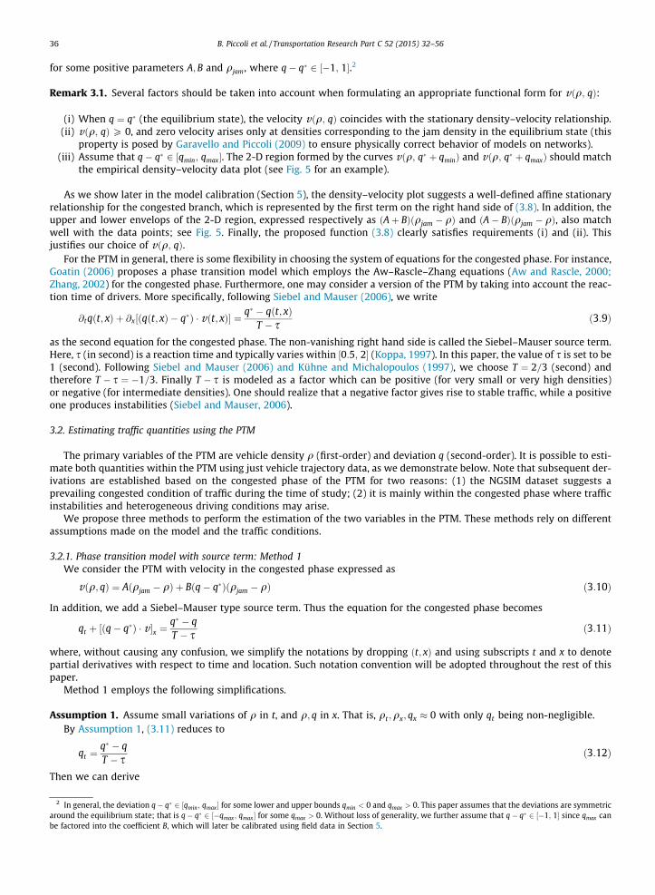
property is posed by Garavello and Piccoli (2009) to ensure physically correct behavior of models on networks).(iii) Assume that q� q� 2 ½qmin; qmax�. The 2-D region formed by the curves vðq; q� þ qminÞ and vðq; q� þ qmaxÞ should match

the empirical density–velocity data plot (see Fig. 5 for an example).

As we show later in the model calibration (Section 5), the density–velocity plot suggests a well-defined affine stationaryrelationship for the congested branch, which is represented by the first term on the right hand side of (3.8). In addition, theupper and lower envelops of the 2-D region, expressed respectively as ðAþ BÞðqjam � qÞ and ðA� BÞðqjam � qÞ, also matchwell with the data points; see Fig. 5. Finally, the proposed function (3.8) clearly satisfies requirements (i) and (ii). Thisjustifies our choice of vðq; qÞ.

For the PTM in general, there is some flexibility in choosing the system of equations for the congested phase. For instance,Goatin (2006) proposes a phase transition model which employs the Aw–Rascle–Zhang equations (Aw and Rascle, 2000;Zhang, 2002) for the congested phase. Furthermore, one may consider a version of the PTM by taking into account the reac-tion time of drivers. More specifically, following Siebel and Mauser (2006), we write

2 In garoundbe facto

@tqðt; xÞ þ @x½ qðt; xÞ � q�ð Þ � vðt; xÞ� ¼ q� � qðt; xÞT � s

ð3:9Þ

as the second equation for the congested phase. The non-vanishing right hand side is called the Siebel–Mauser source term.Here, s (in second) is a reaction time and typically varies within ½0:5; 2� (Koppa, 1997). In this paper, the value of s is set to be1 (second). Following Siebel and Mauser (2006) and Kühne and Michalopoulos (1997), we choose T ¼ 2=3 (second) andtherefore T � s ¼ �1=3. Finally T � s is modeled as a factor which can be positive (for very small or very high densities)or negative (for intermediate densities). One should realize that a negative factor gives rise to stable traffic, while a positiveone produces instabilities (Siebel and Mauser, 2006).

3.2. Estimating traffic quantities using the PTM

The primary variables of the PTM are vehicle density q (first-order) and deviation q (second-order). It is possible to esti-mate both quantities within the PTM using just vehicle trajectory data, as we demonstrate below. Note that subsequent der-ivations are established based on the congested phase of the PTM for two reasons: (1) the NGSIM dataset suggests aprevailing congested condition of traffic during the time of study; (2) it is mainly within the congested phase where trafficinstabilities and heterogeneous driving conditions may arise.

We propose three methods to perform the estimation of the two variables in the PTM. These methods rely on differentassumptions made on the model and the traffic conditions.

3.2.1. Phase transition model with source term: Method 1We consider the PTM with velocity in the congested phase expressed as

vðq; qÞ ¼ Aðqjam � qÞ þ Bðq� q�Þðqjam � qÞ ð3:10Þ

In addition, we add a Siebel–Mauser type source term. Thus the equation for the congested phase becomes

qt þ ½ðq� q�Þ � v �x ¼q� � qT � s

ð3:11Þ

where, without causing any confusion, we simplify the notations by dropping ðt; xÞ and using subscripts t and x to denotepartial derivatives with respect to time and location. Such notation convention will be adopted throughout the rest of thispaper.

Method 1 employs the following simplifications.

Assumption 1. Assume small variations of q in t, and q; q in x. That is, qt ;qx; qx � 0 with only qt being non-negligible.By Assumption 1, (3.11) reduces to

qt ¼q� � qT � s

ð3:12Þ

Then we can derive

eneral, the deviation q� q� 2 ½qmin; qmax� for some lower and upper bounds qmin < 0 and qmax > 0. This paper assumes that the deviations are symmetricthe equilibrium state; that is q� q� 2 ½�qmax ; qmax � for some qmax > 0. Without loss of generality, we further assume that q� q� 2 ½�1; 1� since qmax canred into the coefficient B, which will later be calibrated using field data in Section 5.


DDt

v ¼ @tv qðt; xÞ; qðt; xÞð Þ þ v � @xv qðt; xÞ; qðt; xÞð Þ ¼ vq � qt þ vq � qt þ v � vq � qx þ vq � qx

� � vq � qt

¼ Bðqjam � qÞ � q� � q

T � s¼ 1

T � sBðqjam � qÞðq� � qÞ ¼ 1

T � sAðqjam � qÞ � v� �

ð3:13Þ

Taking into account only the measurements of v and Dv=Dt, and by introducing variables q̂¼: qjam � q; q̂¼: q� q�, we deducefrom (3.13) that

q̂ ¼ ðqjam � qÞ ¼ 1A

v þ ðT � sÞDvDt

� �ð3:14Þ

q̂ ¼ ðq� q�Þ ¼ �AðT � sÞB

DvDt

v þ ðT � sÞ DvDt

ð3:15Þ

Following our discussion at the end of Section 3.1, we take T � s ¼ � 13. The velocity v is estimated according to (2.2), and the

acceleration Dv=Dt is computed from (2.3).

3.2.2. Phase transition model with source term: Method 2The second method again assumes a Siebel–Mauser source term, and relies on the following assumption.

Assumption 2. Assume that qt; qx � 0.Then Eq. (3.11) becomes

qt þ vxðq� q�Þ ¼ q� � qT � s

ð3:16Þ

We can now write

DvDt¼ v t þ vvx � vqqt þ vvx ¼ vq

q� � qT � s

� ðq� q�Þvx

� �þ vvx ð3:17Þ

Recalling the variables q̂¼: qjam � q; q̂¼: q� q�, we obtain

v ¼ Aðqjam � qÞ þ Bðq� q�Þðqjam � qÞ ¼ q̂ ðAþ Bq̂Þ ð3:18Þ

and deduce from (3.17) and (3.18) that

DvDt� vvx ¼ �vq

q̂T � s

þ q̂vx

� �¼ �Bq̂

q̂T � s

þ q̂vx

� �ð3:19Þ

From (3.18) and (3.19) we immediately get the expressions for q̂ and q̂ in terms of v; vx and DvDt .

q̂ ¼ 1A

v þ ðT � sÞ DvDt

1þ ðT � sÞvxð3:20Þ

q̂ ¼ ABðT � sÞ vvx � Dv

Dt

� v þ ðT � sÞ Dv

Dt

ð3:21Þ

The quantities DvDt ; vx are given by (2.3) and (2.4) respectively. Regarding velocity v, notice that if one approximates it with

(2.1), then

DvDt� vvx �

xðtiþ1Þ � 2xðtiÞ þ xðti�1Þdt2 � xðtiþ1Þ � xðti�1Þ

2dt� 2dt� xðtiþ1Þ � 2xðtiÞ þ xðti�1Þ

xðtiþ1Þ � xðti�1Þ� 0 ð3:22Þ

which renders (3.21) identically zero. To avoid such a trivial case, one should instead approximate v by

vðt2Þ � v1;2 ¼xðt2Þ � xðt1Þ

dt; or vðt2Þ � v2;3 ¼

xðt3Þ � xðt2Þdt

; ð3:23Þ

or use robust numerical differentiation illustrated later in Section 4.2.

3.2.3. Phase transition model without source term: Method 3We consider the original PTM without the Siebel–Mauser type source term:

qt þ ðq � vÞx ¼ 0qt þ ððq� q�Þ � vÞx ¼ 0vðq; qÞ ¼ Aðqjam � qÞ þ Bðq� q�Þðqjam � qÞ

8<: ð3:24Þ

Computation in this case is less straightforward than the previous two as no simplification is made in this case. We start withthe identity

3 Zer


DvDt¼ v t þ v � vx ¼ vq qt þ vq qt þ vðvq qx þ vq qxÞ

Using (3.24), we have

DvDt¼ vqð�qxv � qvxÞ þ vqð�qxv � ðq� q�ÞvxÞ þ vðvqqx þ vqqxÞ ¼ �vx vqqþ vqðq� q�Þ

� ¼ vx Aqþ Bðq� q�Þð2q� qjamÞ

� �ð3:25Þ

Recall the variables q̂ ¼ qjam � q and q̂ ¼ q� q�. Combining (3.25) with the expression of vðq; qÞ and solving for q leads to

q ¼ 1Bq̂

v þ 1vx

DvDt� Aqjam

� �ð3:26Þ

One immediate observation from (3.26) is that q̂ and v þ 1vx

DvDt � Aqjam always have the same sign. Substituting (3.26) into

(3.25), we get

B2qjamq̂2 þ B 2Aqjam �1vx

DvDt� 2v

� �q̂� A v þ 1

vx

DvDt� Aqjam

� �¼ 0 ð3:27Þ

which is a quadratic equation in the variable q̂. The discriminant of such a quadratic equation is

D ¼ 4B2 v þ 12

1vx

DvDt� Aqjam

� �2

þ 4AB2qjam v þ 1vx

DvDt� Aqjam

� �¼ 4B2 v þ 1

21vx

DvDt

� �2

� Aqjamv !

ð3:28Þ

In order for any meaningful real root of (3.27) to exist, a necessary condition is that D is nonnegative; that is,

v þ 12

1vx

DvDt

��P ffiffiffiffiffiffiffiffiffiffiffiffiffiffiffi

Aqjamvq

ð3:29Þ

If the equality holds in (3.29), a real solution of q̂ exists if and only if

v þ 1vx

DvDt� Aqjam < 0 ð3:30Þ

In the case where the strict inequality in (3.29) holds, two distinct roots q̂1 and q̂2 exist. We distinguish between two furthercases:

� If

v þ 1vx

DvDt� Aqjam > 0 ð3:31Þ

Then q̂1q̂2 < 0. Eq. (3.27) has one positive root and one negative root. By (3.26), one should choose the positive root sinceq must be non-negative.� If

v þ 1vx

DvDt� Aqjam 6 0 ð3:32Þ

Then q̂1q̂2 P 0. Eq. (3.27) has two roots with the same sign.3 In view of (3.26) and (3.32) to ensure that q is nonnegative,both q̂1 and q̂2 should be nonpositive and at least one root is negative. This in turn requires that

2Aqjam �1vx

DvDt� 2v > 0 ð3:33Þ

In view of (3.32), a sufficient condition for (3.33) to hold is 1vx

DvDt > 0.

It turns out that the above analysis can be more easily interpreted in a discrete-time and numerical setting. Let us con-sider three consecutive time stamps ti�1; ti; tiþ1. First, notice that

1vx

DvDt� dt

2� xðtiþ1Þ � xðti�1Þxðtiþ1Þ � 2xðtiÞ þ xðti�1Þ

� xðtiþ1Þ � 2xðtiÞ þ xðti�1Þdt2 ¼ xðtiþ1Þ � xðti�1Þ

2dt� vðtiÞP 0 ð3:34Þ

In light of this calculation, the feasibility condition (3.29) becomes

32

v PffiffiffiffiffiffiffiffiffiffiffiffiffiffiffiAqjamv

q; or v P

49

Aqjam ð3:35Þ

Using (3.34), the decision rule following (3.29) can be explicitly summarized as follows.

o is considered to have both positive and negative signs.


Algorithm 1. PTM without source term

if v < 49 Aqjam then the model has no solution

else if v ¼ 49 Aqjam then q ¼ qj

3 ; q̂ ¼ � A3B

elseif v > 1

2 Aqjam then

q ¼2qjamð2v � AqjamÞ

3v � 2Aqjam þffiffiffiffiffiffiffiffiffiffiffiffiffiffiffiffiffiffiffiffiffiffiffiffiffiffiffiffiffiffiffiffi9v2 � 4Aqjamv

q ; q̂ ¼3v � 2Aqjam þ

ffiffiffiffiffiffiffiffiffiffiffiffiffiffiffiffiffiffiffiffiffiffiffiffiffiffiffiffiffiffiffiffi9v2 � 4Aqjamv

q2Bqjam

else ffiffiffiffiffiffiffiffiffiffiffiffiffiffiffiffiffiffiffiffiffiffiffiffiffiffiffiffiffiffiffiffiq
q ¼
2qjamð2v � AqjamÞ

3v � 2Aqjam �ffiffiffiffiffiffiffiffiffiffiffiffiffiffiffiffiffiffiffiffiffiffiffiffiffiffiffiffiffiffiffiffi9v2 � 4Aqjamv

q ; q̂ ¼3v � 2Aqjam � 9v2 � 4Aqjamv

2Bqjam

end ifend if

Remark 3.2. We note that the above computational procedure does not produce any result if the velocity is below 49 Aqjam.

Such an assumption may be rather restrictive in application, especially for traffic where low speed is prevailing, although thismethod is exact and consistent with the original phase transition model. As we later show in Table 2, Method 3 is more resil-ient to under sampling in estimating q̂ than the other two methods, whenever applicable.

3.3. Estimating power demand and vehicle emission rates

Car emission and/or fuel consumption rates are considered in this section. They belong to high-order quantities as theyare usually expressed as nonlinear functions of instantaneous speed and acceleration (Post et al., 1984; Barth et al., 2007).That is, the emission and/or fuel consumption rates are related to the modal operation of a moving vehicle such as idle,steady-state cruise, acceleration or deceleration. It requires detailed vehicle trajectory data in order to capture these drivingconditions.

It has been shown that fuel consumption is closely related to the engine power expressed as the power demand function(PDF) (Post et al., 1984; Barth et al., 2007), which in turn can be expressed as a nonlinear function of vehicle speed and accel-eration, along with parameters related to road grade, air drag and other physical conditions. One example of such a PDF isprovided in Barth et al. (2007) as

Z ¼ M1000

� v � ðaþ g sin hÞ þ MgCr þr2

v2AcCd

� �� v1000

ð3:36Þ

where Z (in kw) is the power demand; v (in km/h) and a (in km/h/s) denote instantaneous speed and acceler-ation, respectively. M (in kg) is vehicle mass and is chosen uniformly as 1200 in this paper for simplicity;g ¼ 9:81ðm=s2Þ is the gravitational constant; h is the road grade and is chosen to be zero; r ¼ 1:225 (kg/m3)is the mass density of air. Finally, Cr ¼ 0:005; Ac ¼ 2:6 (m2), and Cd ¼ 0:3 denote respectively the rolling resistancecoefficient, the cross-sectional area, and the aerodynamic drag coefficient, and their values are suggested by Chan(1997).

Regarding vehicle emission, we consider hydrocarbon (HC) and employ the model proposed in Ahn et al. (2002). Thatpaper presents a hybrid 3rd-order polynomial regression model with logarithmic transformation where the acceleration case(ða P 0) and the deceleration case (a < 0) are fitted separately. The HC emission rate is modeled as

ln rHC ¼

X3

i¼0

X3

j¼0

Uij � v i � aj if a P 0

X3

i¼0

X3

j¼0

Vij � v i � aj if a < 0

8>>>><>>>>:

ð3:37Þ

where the matrices fUijg3i;j¼0 and fVijg3

i;j¼0 are explicitly given in Ahn et al. (2002), and are omitted here. This modelis shown to better approximate the HC emission for combinations of relatively high speed and acceleration, and arethus chosen here since part of the monitored traffic is highly unstable containing accelerations up to 10 km/h persecond.


Remark 3.3. Here we assume, as in almost all macroscopic traffic models, that all vehicles have the same characteristics, e.g.weight, engine type, size, and so on. The NGSIM dataset contains vehicle type which could potentially improve theestimation accuracy. This is, however, not pursued by this paper as we aim to describe the evolution of traffic at an aggregatelevel with bounded granularity on the characteristics of the flows.

We further note the fact that other types of models for instantaneous emission rate, power demand function and/or fuelconsumption rate can be equally applied to our framework, as long as they are expressible as functions of speed, accelera-tion, and vehicle-specific characteristics. Although employing these alternative models will yield quantitatively differentresults, the general conclusion drawn from this paper will remain valid; that is, estimations with under sampling of the vehi-cle location and lower probe penetration rate tend to misinterpret these quantities (see Sections 6.3 and 8.1), and the degreeof such miscalculation depends on a number of factors, e.g. traffic condition (stable/unstable), vehicle type, and modelparameters.

4. Reconstructing ground-truth data

The NGSIM contains raw data in video format on vehicle trajectories with a high time resolution. Derived vehicle-specificquantities such as velocity and acceleration are also included therein. However, sensing errors are expected to exist, as arederived errors arising from numerical differentiation. There exist a number of ways to pre-process those vehicle trajectorydata via data smoothing techniques and robust numerical differentiation; see Montanino and Punzo (2013) and Punzo et al.(2011) for examples. Based on these prior approaches, we present here two methods for reducing noises inherent in thedataset and reconstructing the ground-truth data for later use.

4.1. Robust smoothing methods

Several standard smoothing techniques are available for improving regularity of the quantities of interest; e.g. the movingaverage method; the LOESS (local regression using weighted linear least squares and a second-degree polynomial model);and the LOWESS (local regression using weighted linear least square and first-degree polynomial model). We refer the readerto Cleveland et al. (1990) and Cleveland and Devlin (1988) for more elaborated discussions. However, these smoothing tech-niques, which are mostly based on least-square regression, are known to be sensitive to outliers, which should ideally beremoved before smoothing is applied. A few generic methods for detecting outliers in a dataset are summarized byBlatná (2005). For the time series of vehicle location, velocity and acceleration in the NGSIM data, removal of the outliersis done in Montanino and Punzo (2013) and Punzo et al. (2011).

For the application described in this paper, we utilize the robust versions of the ‘‘LOESS’’ or ‘‘LOWESS’’ methods, namely‘‘RLOESS’’ or ‘‘RLOWESS’’, which are implemented and documented in the MATLAB Curve Fitting toolbox.4 Taking ‘‘RLOESS’’ asan example, it first smoothes the value at a given point through local regression using nearby data points (the range of thosepoints is determined by a parameter called span); this is precisely the procedure employed by ‘‘LOESS’’. Additionally, the ‘‘RLO-ESS’’ calculates the residuals from the aforementioned regression and assigns a robust weight to each data point within thespan: 8

4 URL

wi ¼1� ri

6MAD

� 2� �2

if jrij < 6MAD

0 if jrijP 6MAD

<: ð4:38Þ

where ri denotes the residual of the ith data point, and MAD (median absolute deviation) is defined as medianðjrijÞ over alldata points. The MAD is a measure of how spread out the residuals are. If ri for a given i is larger than 6MAD, then theith point is considered an outlier and is assigned weight 0. Finally, the regression is applied again to smooth the data, butwith the robust weights (4.38).

Remark 4.1. If one applies the robust local regression method to location, speed, and acceleration data separately, differentdegree of smoothing (span) should be used. The reason is that the regularities of these quantities are decreasing, and witheach differentiation, the error becomes magnified into increasingly larger ones. Moreover, applying the smoothing separatelymeans that these quantities may no longer be consistent as the derivative of the smoothed location is no longer thesmoothed speed, and etc. Such an inconsistency is illustrated further in Fig. 1.

4.2. Regularization of numerical differentiation

It is conventionally acknowledged that finite-difference approximations, such as those expressed by (2.1) and (2.2), tendto amplify noises existing in the subject of numerical differentiation. In some applications, smooth-then-differentiate or dif-ferentiate-then-smooth may not yield satisfactory results (Chartrand, 2011). Instead of applying the smoothing method toindividual trajectories of location, velocity, or acceleration, one alternative is to utilize a numerical differentiation schemethat is robust against noises in the data. One such robust scheme is Tikhonov regularization (Tikhonov, 1963; Chartrand,

: http://www.mathworks.com/help/curvefit/smoothing-data.html.

http://www.mathworks.com/help/curvefit/smoothing-data.html


2011), and it works as follows. Given a function f, its derivative on ½0; T�, denoted by g, is the solution of the following min-imization problem.

5 Motransfor

mingFðgÞ ¼ aRðgÞ þ DFðIg � f Þ ð4:39Þ

where RðgÞ is a regularization term that penalizes the irregularity in g, and it is chosen as the square of the L2 norm of thederivative of g in our study:

RðgÞ¼:Z T

0g0ðsÞj j2 ds

Such a choice forces g to be continuous and reasonably regular by penalizing large values of jg0j. The operator I representsintegration, and IgðtÞ ¼:

R t0 gðsÞds; t 2 ½0; T�. DFðIg � f Þ is a data fidelity term that penalizes the discrepancy between

Ig and f, and it is chosen as the square of the L2 norm of Ig � f . a > 0 is a weighting parameter that balances betweenthe two terms.

In a discrete-time setting, denote by f i and gi the discrete values of f and g respectively, i ¼ 1; . . . ;n. The integration oper-ator is approximated by a rectangular or trapezoidal quadrature and can be written as an affine transformation5 in discretetime:

ðIgÞi : 1 6 i 6 n� �

¼ Ag þ b A 2 Rnn; b 2 Rn

where g ¼ fgi : 1 6 i 6 ng. Moreover, the numerical differentiation g0 can be also represented by an affine transformation:

ðg0Þi : 1 6 i 6 n� �

¼ Cg þ d C 2 Rnn; d 2 Rn

where the dimensions of A, C and b, d may vary depending on the numerical differentiation scheme. The discretized mini-mization problem becomes a quadratic program:

ming

adt � ðCg þ dÞTðCg þ dÞ þ dt � ðAg þ b� f ÞTðAg þ b� f Þ ð4:40Þ

with some minor constraints whenever applicable (such as the non-negativity of v when differentiating x), where dt denotesthe time step size. This mathematical program can be solved efficiently with standard solvers given that the dimension of f org is not too high (no more than a few thousands), which is indeed the case for the NGSIM dataset.

Remark 4.2. Other choices of the regularization term RðgÞ include the L1 norm of the derivative of g, i.e.

RðgÞ ¼Z T

0g0ðsÞj jds ð4:41Þ

In this case, due to the presence of the absolute value, the discrete optimization problem becomes non-smooth. Chartrand(2011) solves this case by applying first-order necessary conditions to the continuous-time problem (4.39), which are thendiscretized. Another choice for RðgÞ is the square of the L2 norm of g (Tikhonov, 1963):

RðgÞ ¼Z T

0gðsÞj j2 ds ð4:42Þ

which suppresses large values of g without necessarily forcing it to be regular. A quadratic program can be formulated in thiscase by taking C to be the identity matrix and d ¼ 0 in (4.40).

4.3. Implementation of the denoising methods

This section presents a numerical study of the two denoising methods mentioned above. We apply the two methods tothe NGSIM dataset with the following chosen parameters. For the robust smoothing method, we apply the ‘‘RLOESS’’ to loca-tion (with span = 0.005), velocity (with span = 0.01) and acceleration (with span = 0.03) separately. We note that by doing so,the trajectories are no longer consistent; e.g. the derivative of the smoothed location is not approximated by the smoothedvelocity. Regarding the robust differentiation method, we apply the regularization in differentiating location with a ¼ 0:01 toget velocity, and then differentiate the acquired velocity with a ¼ 0:05 to get the acceleration. The resulting trajectories arerelatively consistent thanks to the data fidelity term in (4.39). Notice that in both methods, we have applied different degreesof smoothness (span in the first method and a in the second method) to location, velocity and acceleration due to the naturaldegradation of regularity as a result of differentiation.

Fig. 1 compares the denoised velocity and acceleration profiles of the same car obtained by the two methods. A discern-ible difference in the acceleration can be seen while the velocity profiles are similar. We illustrate the qualitative difference

st numerical integration or differentiation operators are linear in the discrete values of the subject function, therefore they can be represented by affinemations.

Fig. 1. Comparison of denoised velocity (top row), acceleration (middle row), and jerk (bottom row) obtained from RLOESS (left column) and regularization(right column). The bottom row only shows the denoised data as the raw data oscillate violently and obstruct the visualization.


between the two acceleration profiles at two distinct time windows. First, at t � 4 s which is marked with a black dot in thefigures, the vehicle experienced a sudden velocity reduction, indicating one or several large negative values in the acceler-ation. This is, however, insufficiently captured by RLOESS as these negative values were likely to be treated as outliers. Theregularized differentiation, on the other hand, captures this negative acceleration. The second time window is roughly½55; 60� s, during which the car is continuously accelerating. This is reflected by the regularization method which predictsan acceleration well above zero during this period. However, the RLOESS method yields some negative acceleration values.Overall, it is confirmed that while both methods yield improved regularity in the estimated quantities, the regularizationmethod is more faithful to the physical interpretation of these quantities, as expected from the theory. The RLOESS some-times treats unusual yet realistic measurements as outliers (such as the sudden speed reduction at t ¼ 4 s). In addition,the regularization method yields acceleration that does not change signs as frequently as the RLOESS, which is consistentwith the expected vehicle performance.

In the last row of Fig. 1, we show the time-trajectories of the jerk (rate of change of the acceleration) obtained from thetwo methods, with span = 0.05 and a ¼ 0:1, respectively. An inspection of the overall estimation of velocity, acceleration andjerk reveals that the two methods yield estimation results that are increasingly different when the order of the underlyingtraffic quantity is higher, which makes sense as the noises are amplified and the regularities are worsened each time whendifferentiation is performed. In addition, the regularization method seems to represent the physics of traffic relatively well,while the RLOESS method may be more resilient to the outliers in the data and sensing errors.

For the study presented in the rest of this paper, we re-construct the ground truth using the following two-step method.We first apply the RLOESS method with span = 0.01 to smooth the location data. Then, we use the smoothed location to per-form robust numerical differentiations following Section 4.2, and the resulting velocity (with a ¼ 0:01) and acceleration(with a ¼ 0:03) are taken as the ground truth.

Remark 4.3. The proposed two-step method yields location x and acceleration a that are consistent in the sense of

regularized differentiation, rather than finite-difference differentiation i:e: ai ¼ xiþ1�2xiþxi�1

dt2

� �. One could devise a further step

to construct another location data ~x that is consistent with a in the finite-difference sense, although this step is not anecessity for our study. The way to do this is to treat acceleration a as the ground truth and construct ~x according to thefollowing optimization problem

~x ¼ argminy

y� xk k2 subject to D2y ¼ a

On−RampPowell Street

Ashby AveOn−Ramp

2 3 4 5 6

1

Study Area

1650’

Camera

Fig. 2. The study area, spanning 1650 feet in length in the northbound of Interstate 80 located in Emeryville, CA.


where the matrix operation D2y represents the second-order differentiation of y using finite difference (2.3), which isexpressible as a linear operator. The constraint D2y ¼ a is the consistency condition, and the objective is a data fidelity con-dition that minimizes the discrepancy between ~x and the smoothed data x. This minimization problem can be formulated asa quadratic program.

Applying this method will yield a single trajectory ~x, whose second derivative (in the finite difference sense) is a, thesmoothed acceleration from our two-step method.

5. Model calibration

Before we implement the computational procedures proposed in Section 3, we need to estimate the values for A, B andqjam appearing in (3.10) and subsequent calculations. We use the available NGSIM dataset to calibrate these modelingparameters.

5.1. Description of vehicle trajectory data

The NGSIM program focuses on the northbound of I-80 located in Emeryville, CA. The highway segment of interest spans1650 feet in length with an on-ramp at Powell Street and an off-ramp at Ashby Avenue; see Fig. 2. The highway segment hassix lanes with the leftmost lane being a high-occupancy vehicle (HOV) lane, and the rightmost one being a merge/diverge lane.Data were collected using several video cameras. Digital video images were collected over an approximately five-hour periodfrom 2:00 pm to 7:00 pm on April 13, 2005. Complete vehicle trajectories transcribed at a resolution of 1 frame per 0.1 s,along with vehicle type, lane identification and so forth were recorded and processed over three time slots: 4:00–4:15 pm, 5:00–5:15 pm, and 5:15–5:30 pm. The layout of the study area is shown in Fig. 2.

5.2. Estimating the density–flow relationship

We begin with estimating the density–flow relationship (3.8) needed for the congested phase represented by Eq. (3.6).Unlike the LWR model where the density–flow relation is expressed as a single-valued function, the fundamental diagramcorresponding to the congested phase of the PTM is a multi-valued map. This means that a given density q corresponds to a

Cij

xj+1

xj

xj−1

ti+1titi−1ti−2

Fig. 3. Estimation of density and velocity inside a bin. The curves represent vehicle trajectories where the locations are recorded at the solid dots. For thedepicted scenario, the occupancy of bin Cij is three vehicles; the average velocity is taken as the mean of velocities measured/calculated at the four dotsinside Cij .


range of velocities vðq; qÞ; q� q� 2 ½�1; 1�. In order to identify this multi-valued function, we partition the temporal-spatialdomain into small bins Cij¼

: ½ti�1; ti� ½xj�1; xj�; i ¼ 1; . . . ; NT ; j ¼ 1; . . . ; NX where i and j indicate the time step and the spatialstep respectively. The average density associated with Cij is estimated by the number of vehicles whose trajectories indicatetheir presence in the road segment ½xj�1; xj� during time interval ½ti�1; ti�. The velocity inside Cij is calculated as the mean of allvelocity measurements collected within this bin. Fig. 3 illustrates such a procedure. The dimension of the bins used to con-struct the density–flow relation in the congested phase is 4 (seconds) 400 (feet).

The flow within Cij is calculated as the product of the density and the average velocity. The resulting density–flow anddensity–velocity plots for the entire study period are shown in Fig. 4.

5.3. Constructing the congested region in the fundamental diagram

Eq. (3.10) suggests an affine density–velocity relationship v ¼ Aðqjam � qÞwhen the perturbation q� q� is zero, a situationreferred to as the equilibrium state. To determine A and qjam, we conduct the following procedure. First, we visually removethe outliers in the density–velocity plot; see Fig. 4. Then, we conduct a linear regression to determine the equilibrium den-sity–velocity relationship: v ¼ Aðqjam � qÞ. The best fit is v ¼ �287:25qþ 62:61, which implies A ¼ 287:25

(foot2=vehicle=second) and qjam ¼ 0:218 (vehicle/foot). The linear fit is indicated as the red solid line in the right part of

Fig. 5.It remains to determine B, which effectively dictates the width of the 2-D area in the congested domain of the fundamen-

tal diagram. Since q� q� 2 ½�1; 1�, the upper and lower envelops of the congested domain in the density–velocity relation-ship, depicted in the right part of Fig. 5, are respectively

Fig. 4.functiolegend,

Aðqjam � qÞ þ Bðqjam � qÞ ðupper envelopÞAðqjam � qÞ � Bðqjam � qÞ ðlower envelopÞ

(

0 0.05 0.1 0.15 0.2 0.250

0.5

1

1.5

2

2.5

3

3.5

4

4.5

5

Density (vehicle/foot)

Flow

(ve

hicl

e/se

cond

)

0 0.05 0.1 0.15 0.2 0.250

10

20

30

40

50

60


Vel

ocity

(fo

ot/s

econ

d)

The congested branch of the density–flow relationship (left) and the density–velocity relationship (right) for the PTM, both expressed as set-valuedns of density. The red crosses represent outliers that are discarded in the curve fitting. (For interpretation of the references to color in this figurethe reader is referred to the web version of this article.)

0 0.05 0.1 0.15 0.2 0.250

0.5

1

1.5

2

2.5

3

3.5

4

4.5

5


Flow

(ve

hicl

e/se

cond

)Data plots

Upper envelop

Lower envelop

0 0.05 0.1 0.15 0.2 0.250

10

20

30

40

50

60


Vel

ocity

(fo

ot/s

econ

d)

Data plotsEquilibrium stateUpper envelop Lower envelop

Fig. 5. The fitted density–flow relationship (left) and density–velocity relationship (right) with A ¼ 287:25 (foot2=vehicle=second), B ¼ 137

(foot2=vehicle=second), and qjam ¼ 0:218 (vehicle/foot).


Since A and qjam are known, we choose the smallest value of B such that >95% of the data points fall within the area formed bythe upper and lower envelopes; see the right part of Fig. 5. This yields B ¼ 137 (foot2

=vehicle=second), and the resultingenvelops are shown in the right part of Fig. 5. Consequently, the upper and lower envelops in the density–flow relationshipare uniquely determined as

Table 1Relativerespect

N

v trukvk

atrukak

Aðqjam � qÞqþ Bðqjam � qÞq ðupper envelopÞAðqjam � qÞq� Bðqjam � qÞq ðlower envelopÞ

(;

which are quadratic curves (parabolas); see the left part of Fig. 5.

6. Estimating traffic quantities along vehicle trajectories

In this section, we present the estimation results associated with various first- and higher-order traffic quantities alongvehicle trajectories. Those quantities include: velocity and acceleration given by (2.2) and (2.3), vehicle density given by(3.14), (3.20) or Algorithm 1, deviation given by (3.15), (3.21) or Algorithm 1, and the power demand and HC emission rategiven by (3.36) and (3.37). Different sampling frequencies will be used to investigate the deterioration of estimation qualitycaused by under sampling. Recall that the vehicle locations in the NGSIM raw dataset are recorded every 0.1 s. In order toaccommodate different sampling frequencies, we consider an integer N and extract data from the raw dataset every N points.For example, N ¼ 30 implies a sampling period of 0:1 30 ¼ 3 s. We then compute the relative L1 error between the quan-tities estimated with N > 1 and the ground truth.

All the numerical results reported below are based on data collected during 4:00–4:15 pm and 5:00–5:30 pm. The totalnumber of vehicles involved in these time periods is 5677. The results summarized in tables or figures below are based ondata in the entire study period of 45 min unless otherwise stated. As we have explained in detail in Section 4, the ground-truth quantities used throughout our numerical experiments are re-constructed using a combined approach of smoothingand robust differentiation.

6.1. Velocity and acceleration

Vehicle speed and acceleration are among the most fundamental traffic quantities. Following the steps explained at thebeginning of this section, we compute and summarize in Table 1 the mean and standard deviation of the relative L1 errors forthe velocity and acceleration. Overall, the estimation of both these quantities deteriorates with under sampling. Moreover,the acceleration estimation is more susceptible to under sampling than velocity estimation. This is because much of the

errors of velocity and acceleration estimation using different sampling frequencies. v true and atrue denote the ground-truth velocity and accelerationively; vN and aN denote the reconstructed velocity and acceleration with different values of N.

Mean (%) Standard deviation (%)

10 20 30 10 20 30

e � vNkL1

truekL1

2.15 4.35 6.41 0.63 1.46 2.53

e � aNkL1

truekL120.91 47.43 63.51 6.23 11.49 11.94


higher-order variation in the acceleration takes place on a smaller time scale, as confirmed by the poor regularity in theacceleration profile (see, for example, Figs. 1 and 6), and cannot be sufficiently captured with under sampling. Fig. 6 showsone example of the reconstructed velocity and acceleration of the same car by using different values of N. It is confirmed thatthe fitting of velocity shows an overall improvement over the fitting of acceleration, which is caused by the poorer regularityin the latter quantity, i.e. more oscillations are observed in a short time period.

6.2. Vehicle density and deviation

The density q̂ and deviation q̂ are estimated by (3.14) and (3.15) (Method 1), (3.20) and (3.21) (Method 2), or Algorithm 1(Method 3) under various assumptions on the source term and traffic flow conditions. The means and standard deviations ofthe relative L1 errors are summarized in Table 2.

All three methods show qualitatively similar results: The estimation of the first-order quantity (density) is more accuratethan the estimation of the second-order quantity (deviation) under the same condition. Moreover, both estimates deteriorateas the sampling frequency decreases. These results show some similarities to the estimation of velocity and acceleration(Section 6.1). Furthermore, method 2 shows slightly worsened yet satisfactory estimation for density q̂. On the other hand,its estimation of q̂ suffers significantly with under sampling (all errors are greater than 100% and thus are not shown in thetable). As we have explained in Eq. (3.22) that the finite-difference approximation of the quantity Dv

Dt � vvx is zero. Even withmodified finite-difference schemes such as (3.23) or robust differentiation schemes mentioned in Section 4, such a quantityis likely to be very small, causing Eq. (3.21) to yield q̂ with small magnitude and small L1 norm, and consequently, leading tolarge relative L1 errors. This shows that Method 2 is not robust enough in handling the deviation q̂.

Interestingly, the estimation errors for q̂ in the no-source case (Method 3) are much lower than Method 1. This is due tothe exact approach employed by Method 3 without simplification regarding the traffic dynamics, as opposed to the othertwo approaches. However, recall that Method 3 works only when v > 4

9 Aqjam � 27:83 (foot/s). As shown by the right halfof Fig. 4, the majority of the speed measurements fall below this value. In order to apply this method, we select vehicleswhose trajectories indicate at least one non-trivial period (over 20 s), during which the speed is uniformly above27.83 foot/s, and then apply Algorithm 1 to these periods. The total number of vehicles involved in this computation is1628 (out of 5677 in total). We conclude that the applicability of Algorithm 1 for the no-source case is limited, althoughit yields a more accurate estimation of the deviation than the other two methods.

Fig. 7 shows one example of the reconstructed density and deviation profiles along a single vehicle trajectory, for threedifferent sampling frequencies (N ¼ 10; 20; 30). First of all, a comparison of these cases leads to a similar conclusion regard-ing the deterioration of estimating first- and second-order quantities as before. Moreover, one can clearly observe, from bothground-truth and reconstructed q̂ ¼ q� q�, that the vehicle frequently experienced changes in the traffic conditions,between below-equilibrium speed (q� q� < 0) and above-equilibrium speed (q� q� > 0). Such a characteristic of congested,unstable traffic cannot be captured by first-order models such as the LWR model as it describes only the equilibrium speed asa function of density.

0 20 40 60 800

20

40

Time (s)

Vel

ocity

(fo

ot/s

)

0 20 40 60 80−5

0

5

10

Time (s)

Acc

eler

atio

n (f

oot/s

2 )

0 20 40 60 800

20

40

Time (s)

Vel

ocity

(fo

ot/s

)

0 20 40 60 80−5

0

5

10

Time (s)

Acc

eler

atio

n (f

oot/s

2 )

0 20 40 60 800

20

40

Time (s)

Vel

ocity

(fo

ot/s

)

0 20 40 60 80−5

0

5

10

Time (s)

Acc

eler

atio

n (f

oot/s

2 )

Ground truth N=10 Ground truth N=10



Fig. 6. The ground-truth vs. estimated velocity (left column) and acceleration (right column) of the same vehicle, using different sampling frequencies(N ¼ 10; 20; 30).

Table 2Estimation of q̂ and q̂ based on the phase transition model with Methods 1–3. q̂true and q̂true represent the ground-truth quantities estimated using the ground-truth location, velocity and acceleration re-constructed in Section 4. q̂N and q̂N denote the estimated quantities with under sampling. The estimation of q̂ withMethod 2 is not shown as the errors are above 100%.

N Mean (%) Standard deviation (%)

10 20 30 10 20 30

q̂true � q̂Nk kL1

q̂truek kL1

Method 1 2.15 4.55 6.64 0.63 1.62 2.70Method 2 3.56 6.70 9.35 1.35 2.73 4.08Method 3 7.19 13.80 19.39 7.48 14.37 19.46

q̂true � q̂Nk kL1

q̂truek kL1Method 1 20.91 54.41 69.32 6.23 10.96 10.23Method 2 – – – – – –Method 3 12.80 27.58 40.75 6.30 13.43 19.22

0 20 40 60 800

0.1

0.2

Time (s)

Den

sity

(ve

h/fo

ot)

0 20 40 60 80−0.5

0

0.5

Time (s)D

evia

tion

q−q*

0 20 40 60 800

0.1

0.2

Time (s)

Den

sity

(ve

h/fo

ot)

0 20 40 60 80−0.5

0

0.5

Time (s)

Dev

iatio

n q−

q*

0 20 40 60 800

0.1

0.2

Time (s)

Den

sity

(ve

h/fo

ot)

0 20 40 60 80−0.5

0

0.5

Time (s)

Dev

iatio

n q−

q* Ground truth N=30

Ground truth N=30

Ground truth N=20

Ground truth N=20

Ground truth N=10

Ground truth N=10

Fig. 7. The ground-truth and estimated density (left column) and deviation (right column) profiles along the same vehicle trajectory, using differentsampling frequencies.

Table 3Estimations of the power demand functions Z and the hydrocarbon emission rate rHC based on vehicle trajectories. Subscripts true and N denote the ground-truth quantity and the reconstructed quantity, respectively.

N Mean (%) Standard deviation (%)

10 20 30 10 20 30

rHCtrue � rHC

N

L1

rHCtrue

L1

13.39 23.58 27.30 16.77 24.69 24.70

Ztrue � ZNk kL1

Ztruek kL118.69 44.93 60.42 4.95 9.36 10.47


6.3. Emission rate and power demand function

The HC emission rate and the power demand function are estimated according to (3.37) and (3.36) respectively, wherethe velocity v and acceleration a are approximated by (2.2) and (2.3). Table 3 summarizes the relative L1 errors in estimatingthe HC emission rate rHC and the power demand Z, when different sampling frequencies are employed.Overall, estimation of these higher-order quantities suffer from under sampling since higher-order variations in the accel-eration profiles are ignored, as expected from Section 6.1. Moreover, the deterioration in the accuracy seems most significantwhen the sampling period increases from N ¼ 10 (1 s) to N ¼ 20 (2 s), which suggests that the sampling period should ideally


be well below 2 s in order to capture these quantities. This can be confirmed from Fig. 8, which shows both ground-truth andestimated rHC and Z associated with the same vehicle. We see that while N ¼ 10 captures the variations in emission rate andpower demand relatively well, N ¼ 20 or 30 causes the estimation to miss the majority of the peak values. Finally, a com-parison between rHC and Z for the same value of N reveals that the errors in the former case is much smaller. The reasonis that while both estimates misinterpret the high variations by similar amount, the time-trajectory of rHC is uniformly abovesome positive value while the time-trajectory of Z remains centered at zero. Therefore, the relative L1 error for rHC tends to besmaller.

7. Estimating Eulerian quantities

The previous section is mainly concerned with traffic quantities associated with a Lagrangian particle; i.e. a moving car. Itwould be desirable to further explore the effect of under sampling in an Eulerian framework; that is, we will study trafficquantities represented on the spatial–temporal domain. We are also prompted to examine how the estimating error dependson the penetration rate of probe vehicles (mobile sensors), in addition to the sampling frequency. The Eulerian traffic quan-tities studied in this section include vehicle density and deviation. Vehicle emission rate will be studied in the next Section.

7.1. Estimating vehicle densities

The procedure for estimating Eulerian density based on vehicle trajectory data and the phase transition model is illus-trated as follows. We consider again the temporal-spatial bins Cij; i ¼ 1; . . . ;NT ; j ¼ 1; . . . ;NX , each expressed as a productof intervals ½ti�1; ti� ½xj�1; xj�. Recall that given a discrete-time trajectory of a vehicle:

. . . ; xðsk�1Þ; xðskÞ; xðskþ1Þ; . . .

where fskg is a fixed time grid, one can estimate the velocity vðskÞ, acceleration aðskÞ, and the Lagrangian density q sk; xðskÞð Þusing techniques elaborated in Sections 2 and 3. In order to estimate the average density of Cij, we search for the probe vehi-cles whose trajectories intersect Cij. Then the density qij associated with Cij is estimated as the average of qðsk; xðskÞÞ for all ksuch that ðsk; xðskÞÞ 2 ½ti�1; ti� ½xj�1; xj�.

One example of such a calculation is presented in Fig. 9, where we utilize vehicle trajectories with a sampling period ofN ¼ 30 (3 s) and a 50% probe penetration rate to perform the estimation of bin-based densities, which is then compared withthe densities obtained from N ¼ 1 and a 100% penetration rate. Fig. 9 shows consistency between the two density estima-tions. Notice from the bottom of Fig. 9 that a few bins are marked with dark blue, which means that they do not haveany valid location measurements that support the computation of density values. We call these bins inactive, which areautomatically assigned zero density and indicated by dark blue in Fig. 9. It is expected that as the penetration rate andthe sampling frequency decrease further, the number of inactive bins will increase drastically. To avoid this, one shouldchoose the dimension of a bin reasonably large to ensure having at least some valid measurements inside each bin. In

0 20 40 60 800

2

4

6

Time (s)

rHC

(m

g/s)

0 20 40 60 800

2

4

6

Time (s)

rHC

(m

g/s)

0 20 40 60 800

2

4

6

Time (s)

rHC

(m

g/s)

0 20 40 60 80−200

0

200

400

Time (s)

Pow

er d

eman

d (k

w)

0 20 40 60 80−200

0

200

400

Time (s)

Pow

er d

eman

d (k

w)

0 20 40 60 80−200

0

200

400

Time (s)

Pow

er d

eman

d (k

w)

Ground truth

N=10

Ground truth

N=20

Ground truth

N=30

Ground truth N=10

Ground truth N=20

Ground truth N=30

Fig. 8. Ground-truth and estimated hydrocarbon emission rate (left column) and power demand function (right column).


our numerical results presented in the next section, the dimension of a bin is chosen to be 4 (seconds) 400 (feet). We shalluse the phase transition model and the LWR model to perform Eulerian density estimation with a range of sampling frequen-cies and probe penetration rates.

7.2. Density estimation: a comparative study of the PTM and the LWR mdoel

In this section we evaluate the performance of the aforementioned estimation method in the presence of insufficient datacoverage, that is, when the penetration rate and the sampling frequency are low. The purpose is to evaluate and justify theeffectiveness of the proposed computational procedure, and to identify certain range of penetration rates and sampling fre-quencies such that the domain of study is sufficiently covered and the estimation error remains reasonably low.

In addition, we propose a comparative study of second-order models (the phase transition model) and first-order models(the LWR model) in terms of their accuracies in density estimation. For the LWR model (3.5), we need to calibrate the single-valued fundamental diagram (FD) in view of the density–flow relationship shown in Fig. 4. To do this, we first consider anaffine congested branch by applying a least-square linear regression to the density–flow plot after removing the outliers; seethe left figure of Fig. 10. The result, however, was rather peculiar (with very large qjam) as shown in Fig. 10. Applying thisaffine FD leads to substantial error in the estimation and thus is not adopted here. We instead employ the equilibrium den-sity–flow relationship from the PTM case (notice that this relationship is obtained from a least-square linear regression of thedensity–velocity plots; see the right part of Fig. 10):

Fig. 9.rate. Thblue in

flow ¼ Aqðqjam � qÞ

where A ¼ 287:25 (foot2/vehicle/s), qjam ¼ 0:218 (vehicle/foot); see Fig. 10 for the curve fitting result, where the utilizedcurves are indicated with solid red lines.

It can be seen that the single-valued density–flow relationship, no matter how derived, does not capture deviation fromthe equilibrium states, i.e. the scattered measurements in a 2-D region. The LWR model treats the traffic stream as stable andhomogeneous; as a result, second-order variations such as acceleration/deceleration are not sufficiently captured. In order toapply the LWR model to perform density estimation, we first utilize the probe trajectory data to obtain information of theinstantaneous speed v; then we evaluate the function q ¼ g�1ðvÞ to get the estimated density value, where gðqÞ is the invert-ible density-speed relationship depicted on the right half of Fig. 10. The rest of the procedure is the same as the PTM case.

The ground-truth density associated with each spatial–temporal bin is calculated by counting the number of vehiclespresent in that bin, using ground-truth trajectory data. The ground-truth density is then compared with the estimated den-sities obtained with a combination of lower sampling frequencies and lower penetration rates. The relative errors for allactive bins are averaged and shown in Table 4 for period 4:00–4:15 pm, in Table 5 for period 5:00–5:15 pm, and in Table 6for period 5:15–5:30 pm. Here in these calculations, Method 1 is employed by the PTM-based estimation. The results withMethod 2 is qualitatively similar and are omitted here.

From all three tables, we notice that the penetration rate of probe vehicles has a stronger effect on the estimationaccuracy than the sampling frequency. This again confirms our observation that, when it comes to estimating first-order

Reconstruction of cell densities (in vehicle/foot) during 4:00–4:15 pm. The top figure shows the density obtained with N ¼ 1 and 100% penetratione bottom figure shows the estimated density with N ¼ 30 and penetration rate = 50%. The inactive bins are assigned zero density and marked as darkthe figure. (For interpretation of the references to color in this figure legend, the reader is referred to the web version of this article.)

0 0.05 0.1 0.15 0.2 0.25 0.30

0.5

1

1.5

2

2.5

3

3.5

4

4.5

5


Flow

(ve

hicl

e/se

cond

)

Density−flow plots

Linear regression

PTM equilibrium state

0 0.05 0.1 0.15 0.2 0.25 0.30

10

20

30

40

50

60


Vel

ocity

(fo

ot/s

econ

d)

Density−velocity plots

From affine FD

Linear regression

Fig. 10. Fitting of the congested branch of the LWR fundamental diagram. Our study uses the equilibrium density–velocity or density–flow relationshipfrom the PTM case, which are indicated as solid red lines. (For interpretation of the references to color in this figure legend, the reader is referred to the webversion of this article.)


quantities, under sampling does not affect the accuracy as much as the penetration rate. On the other hand, the substantialvariation in the penetration rate, from 100% to 2%, has caused approximately 14% difference in both PTM-based and LWR-based estimations. Moreover, the PTM-based estimation is more accurate than the LWR-based estimation for any given com-bination of penetration rate and sampling frequency, and the difference is more evident for lower penetration rates. This isexplained by the fact that the LWR model only captures the equilibrium state of the density–flow or density–velocity rela-tionship, and ignores possible deviations from such an equilibrium state. As shown in Fig. 10, the congested traffic is unstableand likely to deviate from the equilibrium state. Thus, the second-order model (PTM) is able to capture these deviationsthrough the use of the variable q and a multi-valued fundamental diagram. As a result, the second-order model is able toestimate vehicle densities more accurately than the LWR model for congested highway traffic.

7.3. Deviation of traffic from equilibrium

In this section we calculate q� q�, the indicator of the deviation of a vehicle speed from the equilibrium speed of sur-rounding vehicles. The PTM with a multi-valued FD allows disequilibrated traffic and complex waves, commonly observedin congested highway traffic, to be described and modeled. This is in contrast to the LWR model which captures only theequilibrium traffic states.

Using a similar procedure described in Section 7.1, we compute the quantity q̂ ¼ q� q� using formula (3.15). It has beenshown in Table 2 that the estimation of q̂ is very susceptible to under sampling and, potentially, lower probe penetration aswell, we utilize the entire ground-truth data (N ¼ 1, penetration rate = 100%) to reconstruct the bin-based q̂, following a sim-ilar procedure described in Section 7.1. The result is shown in Fig. 11 for the traffic during 5:00–5:30 pm. It can be seen fromthe top figure showing the density that the traffic was significantly congested and multiple shock waves were present andpropagated with positive or negative speeds. The picture in the middle shows the bin-based q� q�, which takes value in½�1; 1�. We observe that traffic stayed close to equilibrium (q� q� ¼ 0) where density was relatively low (typically below0.16 vehicle/foot). However, significant deviation occurred with higher traffic densities. Furthermore, the presence of thesehigh densities was accompanied by a mixture of above-equilibrium (q� q� > 0) and below-equilibrium (q� q� < 0) states.

Table 4Comparison of the PTM and LWR models in estimating bin-based densities using different sampling frequencies and penetration rates, for the period 4:00–4:15 pm. ‘‘Coverage rate’’ is the ratio of the number of active bins and the total number of bins.

Sampling period Probe vehicle penetration rate

100 % 50 % 20 % 10 % 5 % 2 %

PTM Average error (%) N ¼ 10 8.74 9.25 11.04 13.40 16.95 21.53N ¼ 20 8.86 9.44 11.19 13.48 17.05 21.26N ¼ 30 8.99 9.57 11.41 13.74 17.25 21.04

Coverage rate (%) 100.00 100.00 100.00 99.83 97.67 79.70

LWR Average error (%) N ¼ 10 12.66 13.29 15.47 18.37 22.45 27.52N ¼ 20 12.58 13.24 15.41 18.29 22.33 27.04N ¼ 30 12.43 13.03 15.31 18.26 22.26 26.44

Coverage rate (%) 100.00 100.00 100.00 99.83 97.67 79.70



100 % 50 % 20 % 10 % 5 % 2 %


Coverage rate (%) 100.00 100.00 100.00 99.97 98.57 82.88

LWR Average error (%) N ¼ 10 10.78 11.26 12.24 14.24 17.85 23.09N ¼ 20 10.96 11.44 12.44 14.44 17.91 22.95N ¼ 30 11.44 11.93 12.93 14.81 18.29 22.80

Coverage rate (%) 100.00 100.00 100.00 99.97 98.57 82.88



100 % 50 % 20 % 10 % 5 % 2 %


Coverage rate (%) 100.00 100.00 100.00 99.98 98.99 85.56LWR Average error (%) N ¼ 10 12.69 12.87 13.49 14.45 16.82 21.03

N ¼ 20 12.85 13.02 13.64 14.59 16.95 20.85N ¼ 30 13.01 13.17 13.84 14.77 17.11 20.72

Coverage rate (%) 100.00 100.00 100.00 99.98 98.99 85.56

Fig. 11. Space–time diagram of the ground-truth vehicle density (top), signed deviation q� q� (center), and unsigned deviation jq� q�j (bottom). Thedeviations are calculated according to (3.15).



We note that inside the same bin, above-equilibrium and below-equilibrium traffic may be present simultaneously;therefore, averaging q� q� within the same bin does not fully capture the deviation. Thus, we further compute the bin-basedquantity jq� q�j 2 ½0; 1�, and the result is shown in the bottom picture of Fig. 11. Similar to the signed deviation q� q�, theunsigned deviation jq� q�j suggests a strong correlation with the vehicle density. This is consistent with the establishedobservation that congested highway traffic tends to be unstable, due to inhomogeneous driving behavior (Laval andLeclercq, 2010) and the propagation of disturbances (Blandin et al., 2012).

8. Estimating instantaneous emission rate

It has been shown in Section 6.3 that the HC emission rate along vehicle trajectories are largely deteriorated by undersampling. Such significant error is caused by the high variation in the acceleration profile. However, it is expected that whenaggregated on a cell or link level, the estimation accuracy of these quantities may improve even with large sampling periods.To confirm such an observation, we will next perform Eulerian-based HC emission estimation.

8.1. Bin-based estimation with insufficient data coverage

The bin-based emission rate can be estimated as follows. We first calculate the density qij for bin Cij following the pro-cedure illustrated in Section 7.1 using Method 1. Secondly, we use available vehicle trajectories to compute rHCðsk; xðskÞÞusing formula (3.37). Then all rHCðsk; xðskÞÞ that fall within Cij are collected and averaged, which give rise to the averageinstantaneous HC emission rate per vehicle in this bin. Finally, this rate is multiplied by the number of vehicles presentin this bin, which is given by the density, to yield the HC emission rate of Cij.

Following this procedure, we perform the Eulerian estimation of rHC for a combination of lower sampling frequencies andpenetration rates, which are then compared with the ground truth. The bin-based relative errors are averaged and shown inTable 7 for the period 5:00–5:30 pm. Compared to the Lagrangian (single-vehicle) estimation, the Eulerian estimation showsimproved accuracy due to the effect of spatial-temporal aggregation; the reader is referred to Table 3 for a comparison of theresults. Interestingly, the influence of under sampling is reduced as the penetration rate becomes lower. This may beexplained from the following two potential sources of error:

1. the lower sampling frequency that causes high variations in the emission rate to be ignored;2. the computational procedure which directly combines a microscopic emission model with a macroscopic traffic model,

and creates certain mismatch in these very different modeling scales.

It is likely that with very high penetration rate (e.g. 100%, 50%), the first factor is the dominating one, while for lower pen-etration rates the second factor (i.e. representing the emission rate inside a bin using a few microscopic vehicle trajectories)becomes the major source of error.

8.2. Correction factor approach for estimating aggregate emission rate

To further aggregate the hydrocarbon emission rate, we compute the total emission rate on the entire road segment. Thisis done by summing up bin-based rates over all spatial cells for each time interval. An example of these time-dependent ratesare shown in Fig. 12, where the ground-truth rHC is compared with the estimated ones with [N ¼ 10; pr ¼ 50%] and [N ¼ 30and pr ¼ 50%] respectively. From these figures we see that the estimation captures, to some degree, the overall trends of theemission rate, although it tends to underestimate the true value. The reason is that the under sampling overlooks higher-order variations in velocity and acceleration, and thus does not capture surges in the emission rate; a good example canbe seen in Fig. 8. And, such an underestimation is expected to become worse for larger sampling periods, as can be seen froma comparison between the two pictures in Fig. 12.

The numerical result shown in Fig. 12 reveals discernible errors in emission estimation, although the overall time-varyingtrends of rHC is captured using our method. As we argued in Section 8.1, these errors are attributed to two factors, and to

Table 7Estimation of bin-based hydrocarbon emission rate rHC using different sampling periods and penetration rates. The time period is 5:00–5:30 pm. The estimationof vehicle density employs Method 1.


100 % 50 % 20 % 10 %

rHC Average error (%) N ¼ 10 11.04 14.09 19.36 23.67N ¼ 20 16.66 17.96 20.52 23.21N ¼ 30 19.55 20.40 21.75 23.20

Coverage rate (%) 100.00 100.00 100.00 99.88

0 160 320 480 640 800 960 1120 1280 1440 1600100

150

200

250

300

350

400

450

Time (s)rH

C e

mis

sion

rat

e (m

g/s)

Ground−truth

N = 10, pr = 50%

0 160 320 480 640 800 960 1120 1280 1440 1600100

150

200

250

300

350

400

450

Time (s)

rHC

em

issi

on r

ate

(mg/

s)

Ground truth

N = 30, pr = 50%

Fig. 12. Time-dependent HC emission rate on the entire study area (1600 feet in length) for the time period 5:00–5:30 pm. The top figure employs N ¼ 10and 50% penetration rate; the bottom figure employs N ¼ 30 and 50% penetration rate.


resolve these two issues simultaneously, we propose a correction factor approach to adjust the estimation process, which isdemonstrably effective.

8.2.1. Correction factors based on regression modelsWe employ a linear regression approach which finds an appropriate affine relationship between the ground-truth emis-

sion rates and the estimated ones. To demonstrated the hypothesized affine relationship, we plot in Fig. 13 the ground-truthvalue vs. the estimated value for the two cases illustrated in Fig. 12. Each data point on the plane corresponds to one timeinterval; the x-coordinate is the estimated value, and the y-coordinate is the true value. It is generally expected that differentsampling periods and penetration rates require different linear regression coefficients. In fact, the best fit in the two casesare:

Fig. 13.are sho

y ¼ 1:08xþ 23:02 ðN ¼ 10; pr ¼ 50%Þ ð8:43Þ

y ¼ 1:51x� 41:92 ðN ¼ 30; pr ¼ 50%Þ ð8:44Þ

Indeed, the N ¼ 30 case underestimates emission rates more than the N ¼ 10 case, and thus has a larger 1st-order coefficient.We denote by rHC

true the ground truth emission rate, and by rHCest the estimated one. The linear model assumes that

rHCtrue ¼ b0 þ b1rHC

est where b0; b1 2 R. Applying the affine adjustment (8.43) and (8.44) yields the improved estimation depictedin Fig. 14. To rigorously justify the validity and robustness of the proposed correction factor approach, we employ a k-foldcross validation discussed below.

100 150 200 250 300 350 400150

200

250

300

350

400

450

Estimated rHC (mg/s)

Gro

und−

trut

h rH

C (

mg/

s)

Best fit: y = 1.08 x +23.02

100 150 200 250 300 350 400150

200

250

300

350

400

450

Estimated rHC (mg/s)

Gro

und−

trut

h rH

C (

mg/

s)

Best fit: y = 1.51 x − 41.92

Scatter plots of the estimated rHC vs. ground-truth rHC for the entire study area (1600 feet in length) during period 5:00–5:30 pm. The best linear fitswn as solid lines. Left: N ¼ 10;pr ¼ 50%; right: N ¼ 30; pr ¼ 50%.

0 160 320 480 640 800 960 1120 1280 1440 1600100

150

200

250

300

350

400

450

Time (s)rH

C e

mis

sion

rat

e (m

g/s)

Ground truth

N = 10, pr = 50%

With Correction Factor

0 160 320 480 640 800 960 1120 1280 1440 1600100

150

200

250

300

350

400

450

Time (s)

rHC

em

issi

on r

ate

(mg/

s) Ground truth

N = 30, pr = 50%

With Correction Factor

Fig. 14. The adjusted time series of rHC with the correction factors (8.43) and (8.44).


8.2.2. Cross validationWe partition available NGSIM vehicle trajectories into k equal-size subsets. Among the k subsets, a single subset is used as

the training data to obtain the linear coefficients b0 and b1. The rest of the k� 1 subsets are used to validate this affine adjust-ment by calculating the discrepancy between the predicted value (after applying the linear transformation) and the ground-truth value. Such a procedure is repeated k times, each with a distinct training dataset, and the errors from all k repetitionsare averaged. Such a process is known as k-fold cross validation.

We use the absolute relative error jrHCest ðtÞ � rHC

trueðtÞj=jrHCtrueðtÞj to indicate the accuracy of the estimation. A range of sampling

periods and penetration rates are considered as shown in Table 8, which summarizes results of the k-fold cross validation.Notice that for each penetration rate pr, the value k is naturally chosen as 1=pr. It is quite clear from these cross validationresults that applying the correction factor yields significantly improved estimation accuracy.

Remark 8.1. It should be noted that the linear coefficients b0 and b1 employed by the correction factor approach aredetermined separately for each combination of sampling period and penetration rate. The reason is that these factors aredevised to counter the effects of (1) underestimating the emission rates due to lower sampling frequency; and (2) possiblemismatch between the microscopic emission model and macroscopic traffic model. Therefore, the factors must bedetermined separately as the effects (1) and (2) naturally vary in response to N and the penetration rate.

It can be seen that the estimation with correction factors produces errors that are not significantly affected by under sam-pling or lower penetration rate, with a maximum difference of 4% (½N ¼ 10; pr ¼ 50%� vs. ½N ¼ 30; pr ¼ 10%]) over all sce-narios in Table 8. This is in contrast to the case without the correction factors, which has a degradation of accuracy by aslarge as 13% (½N ¼ 10; pr ¼ 50%� vs. ½N ¼ 30; pr ¼ 10%]). This is due to the fact that the correction factors have taken intoaccount misinterpretations of density and emission rate caused by both larger N and smaller pr, and hence the estimationis more resilient to the change in both parameters.

9. Conclusion

This paper presents several approaches to estimate first- and higher-order traffic quantities based on vehicle trajectorydata. It also conducts extensive study of the accuracy of these estimations with respect to the probe penetration rate and

Table 8Cross validation results of the correction factor approach. The errors in the parenthesis are from calculations without any correction factor.


50% 20% 10%

rHC Average error (%) N ¼ 10 10.34 (11.24) 12.34 (15.60) 13.47 (19.77)N ¼ 20 12.21 (17.57) 13.65 (19.77) 14.32 (22.17)N ¼ 30 13.52 (21.89) 14.31 (23.17) 14.39 (24.22)


the sampling frequency of the mobile data. Most existing studies on mobile sensing tend to focus on the penetration rate,while the effect of sampling frequency is rarely studied. We present several data fusion schemes that incorporate vehicletrajectory data into the second-order phase transition model, and perform the estimation of first-order quantities such asspeed and density, and higher-order quantities such as acceleration, deviation (perturbation) and emission rate. The mainfindings are summarized below.

� Various Eulerian and Lagrangian traffic quantities can be estimated via vehicle trajectory data, when the phase transitionmodel (PTM) is employed.� For Lagrangian estimation, the first-order quantities are accurately reconstructed by the proposed method, even with low

sampling frequency. For higher-order Lagrangian quantities, lower sampling frequency significantly reduces the accuracy.� The PTM-based estimation method is extended to perform Eulerian estimation, with varying penetration rate and sam-

pling frequency. The estimation accuracy shows a trend similar to that of the Lagrangian estimation, and deteriorateswith lower penetration rate.� The PTM is compared with the LWR model in estimating Eulerian density with varying sampling frequency and penetra-

tion rate. The results show that the former yields more accurate results due to the fact that it captures second-order devi-ation of traffic, which is frequently observed in congested and unstable traffic and is not described by first-order models.� A correction factor approach is applied to the Eulerian estimation of hydrocarbon emission rate, which significantly

improves the accuracy. The method resolves the underestimation of emission due to insufficient sampling frequency,and the potentially biased emission estimation caused by mismatching modeling scales. As a result, the adjusted estima-tion is less sensitive to the changes in the sampling frequency and penetration rate.

Further research will focus on applying the methodology to urban arterial networks and comparing it with the LWR-based approach. As we mentioned earlier in the introduction, the benefit of applying the PTM to arterial traffic will be some-how limited. However, higher-order variations in acceleration, emission and fuel consumption still need to be captured andquantified in connection with a given traffic flow model, and the effects of sampling frequency and penetration rate on theseestimations should be properly understood in an urban environment.

Acknowledgement

The authors would like to thank two anonymous reviewers for their constructive remarks.

References

Ahn, K., Rakha, H., Trani, A., Van Aerde, M., 2002. Estimating vehicle fuel consumption and emission based on instantaneous speed and acceleration levels. J.Transp. Eng. 128, 182–190.

Argote, J., Christofa, E., Xuan, Y., Skabardonis, A., 2011. Estimation of measures of effectiveness based on Connected Vehicle data. In: Proceedings of the 14thInternational IEEE Conference on Intelligent Transportation Systems. pp. 1767–1772.

Aw, A., Rascle, M., 2000. Resurrection of ‘‘second order’’ models of traffic flow. SIAM J. Appl. Math. 60, 916–938.Ban, X., Herring, R., Hao, P., Bayen, A., 2009. Delay pattern estimation for signalized intersections using sampled travel times. Transp. Res. Rec. 2130, 109–

119.Ban, X., Hao, P., Sun, Z., 2011. Real time queue length estimation for signalized intersections using sample travel times from mobile sensors. Transp. Res. Part

C 19 (6), 1133–1156.Barth, M., An, F., Norbeck, J., Ross, M., 2007. Modal emission modeling: a physical approach. Transp. Res. Rec. 1520, 81–88.Blandin, S., Work, D., Goatin, P., Piccoli, B., Bayen, A., 2011. A general phase transition model for vehicular traffic. SIAM J. Appl. Math. 71, 107–127.Blandin, S., Argote, J., Bayen, A., Work, D., 2012. A phase transition model of non stationary traffic flow: definition, properties and solution method. Transp.

Res. Part B 52, 31–55.Blatná, D., 2005. Robust regression. In: Applications of Mathematics and Statistics in Economy. Wroclav.Chan, C.C., 1997. An overview of power electronics in electric vehicles. IEEE Trans. Ind. Electron. 44 (1), 3–13.Chartrand, R., 2011. Numerical differentiation of noisy, nonsmooth data. ISRN Appl. Math. 2011. http://dx.doi.org/10.5402/2011/164564. Article ID 164564.Cheng, Y., Qin, X., Jin, J., Ran, B., 2012. An exploratory shockwave approach to estimating queue length using probe trajectories. J. Intell. Transp. Syst. 16 (1),

12–23.Christiani, E., de Fabritiis, C., Piccoli, B., 2010. Fluid dynamic approach for traffic forecast from mobile sensor data. Commun. Appl. Ind. Math. 1 (1), 54–71.Claudel, C.G., Bayen, A.M., 2011. Convex formulations of data assimilation problems for a class of Hamilton–Jacobi equations. SIAM J. Control Optim. 49 (2),

383–402.Cleveland, W.S., Devlin, S.J., 1988. Locally weighted regression: an approach to regression analysis by local fitting. J. Am. Stat. Assoc. 83, 596–610.Cleveland, R.B., Cleveland, W.S., McRae, J.E., Terpenning, I., 1990. STL: a seasonal-trend decomposition procedure based on loess. J. Official Stat. 6, 3–33.Colombo, R.M., 2002. Hyperbolic phase transitions in traffic flow. SIAM J. Appl. Math. 63 (2), 708–721.Colombo, R.M., Corli, A., 2002. Sonic hyperbolic phase transition and Chapman–Jouguet detonations. J. Differ. Equ. 184, 321–347.Colombo, R.M., Goatin, P., Priuli, F.S., 2007. Global well posedness of traffic flow models with phase transitions. Nonlinear Anal. 66, 2413–2426.Comert, G., Cetin, M., 2009. Queue length estimation from probe vehicle location and the impacts of sample size. Eur. J. Oper. Res. 197 (1), 196–202.Daganzo, C.F., 1994. The cell transmission model. Part I: a simple dynamic representation of highway traffic. Transp. Res. Part B 28 (4), 269–287.Daganzo, C.F., 1995. Requiem for second-order fluid approximations of traffic flow. Transp. Res. Part B 29 (4), 277–286.Demers, A., List, G.F., Wallace, W.A., Lee, E.E., Wojtowicz, J.M., 2006. Probes as path seekers: a new paradigm. Transp. Res. Rec.: J. Transp. Res. Board 1944,

107–114.Garavello, M., Piccoli, B., 2009. On fluido-dynamic models for urban traffic. Networks Heterogen. Media 4 (1), 107–126.Goatin, P., 2006. The Aw–Rascle vehicular traffic flow model with phase transitions. Math. Comput. 44, 287–303.Herrera, J.C., Work, D.B., Herring, R., Ban, X.J., Jacobson, Q., Bayen, A., 2010. Evaluation of traffic data obtained via GPS-enabled mobile phones: the mobile

century field experiment. Transp. Res. Part C 18 (4), 568–583.

http://refhub.elsevier.com/S0968-090X(14)00363-5/h0005












http://dx.doi.org/10.5402/2011/164564





















Koppa, R.J., 1997. Human factors. In: Monograph on Traffic Flow Theory. U.S. Department of Transportation, Federal Highway Administration, Washington,DC, vol. 1997, pp. (3)1–32. <http://www.tfhrc.gov/its/tft/tft.htm>.

Kühne, R., Michalopoulos, P., 1997. Continuum flow models. In: Monograph on Traffic Flow Theory. U.S. Department of Transportation, Federal HighwayAdministration, Washington, DC, vol. 1997, pp. (5)1–51. <http://www.tfhrc.gov/its/tft/tft.htm>.

Kwon, J., McCullough, B., Petty, K., Varaiya, P., 2007. Evaluation of PeMS to improve the congestion monitoring program. California PATH Research ReportUCB-ITS-PRR-2007-6, Institute of Transportation Studies, University of California, Berkeley, CA.

Laval, J., Leclercq, L., 2010. A mechanism to describe the formation and propagation of stop-and-go waves in congested freeway traffic. Philos. Trans. R. Soc.A: Math. Phys. Eng. Sci. 368, 4519–4541.

Lighthill, M., Whitham, G., 1955. On kinematic waves. II. A theory of traffic flow on long crowded roads. Proc. R. Soc. London Ser. A Math. Phys. Sci. 229(1178), 317–345.

Luspay, T., Kulcsár, B., Varga, I., Zegeye, S.K., De Schutter, B., Verhaegen, M., 2010. On acceleration of traffic flow. In: Proceedings of the 13th InternationalIEEE Conference on Intelligent Transportation Systems (ITSC 2010), Madeira Island, Portugal, September, 2010, pp. 741–746.

Montanino, M., Punzo, V., 2013. Making NGSIM data usable for studies on traffic flow theory: a multistep method for vehicle trajectory reconstruction. In:Proceedings of 92nd TRB Annual Meeting. Washington, D.C., January 13–17, 2013.

Payne, H.J., 1971. Models of Freeway Traffic and Control. Simulation Council.Payne, H.J., 1979. FREFLO: a macroscopic simulation model of freeway traffic. Transp. Res. Rec. 722 (1979), 68–75.Post, K., Kent, J.H., Tomlin, J., Carruthers, N., 1984. Fuel consumption and emission modelling by power demand and a comparison with other models.

Transp. Res. Part A 18 (3), 191–213.Punzo, V., Borzacchiello, M., Ciuffo, B., 2011. On the assessment of vehicle trajectory data accuracy and application to the Next Generation SIMulation

(NGSIM) program data. Transp. Res. Part C 19, 1243–1262.Richards, P.I., 1956. Shockwaves on the highway. Oper. Res. 4 (1), 42–51.Siebel, F., Mauser, W., 2006. On the fundamental diagram of traffic flow. SIAM J. Appl. Math. 66 (4), 1150–1162.Strub, I., Bayen, A., 2006. Weak formulation of boundary conditions for scalar conservation laws: an application to highway traffic modelling. Int. J. Robust

Nonlinear Control, 16 733–748.Tikhonov, A.N., 1963. Regularization of incorrectly posed problems. Sov. Math. Dokl. 4, 1624–1627.Whitham, G.B., 1974. Linear and nonlinear waves. In: Pure and Applied Mathematics. Wiley–Interscience, New York.Work, D.B., Blandin, S., Tossavainen, O.P., Piccoli, B., Bayen, A.M., 2010. A traffic model for velocity data assimilation. Appl. Math. Res. Express 2010 (1), 1–35.Yim, Y., Cayford, R., 2001. Investigation of vehicles as probes using global positioning system and cellular phone tracking: field operational test. California

PATH Working Paper UCB-ITS-PWP-2001-9, Institute of Transportation Studies, University of California, Berkeley, CA.Yuan, Y., Van Lint, J.W.C., Hoogendoorn, S.P., Vrancken, J.L.M., Schreiter, T., 2011. Freeway traffic state estimation using extended Kalman filter for first-order

traffic model in Lagrangian coordinates. In: 2011 IEEE International Conference on Networking, Sensing and Control (ICNSC). IEEE, pp. 121–126.Zhang, H.M., 2002. A non-equilibrium traffic model devoid of gas-like behavior. Transp. Res. Part B 36 (3), 275–290.

http://www.tfhrc.gov/its/tft/tft.htm

http://www.tfhrc.gov/its/tft/tft.htm





















Second order models and traffic data from mobile sensors

Documents

Transcript of Second order models and traffic data from mobile sensors