Evaluation of Traffic Control Devices: Second Year Activities

Technical Report Documentation . Report No. FHWA/TX-06/0-4701-2

2. Government Accession No.

3. Recipient's Catalog No. 5. Report Date October 2005

4. Title and Subtitle EVALUATION OF TRAFFIC CONTROL DEVICES: SECOND YEAR ACTIVITIES

6. Performing Organization Code

7. Author(s) H. Gene Hawkins, Jr., Roma Garg, Paul J. Carlson, and Andrew J. Holick

8. Performing Organization Report No. Report 0-4701-2

10. Work Unit No. (TRAIS)

9. Performing Organization Name and Address Texas Transportation Institute The Texas A&M University System College Station, Texas 77843-3135

11. Contract or Grant No. Project 0-4701 13. Type of Report and Period Covered Technical Report: September 2004–August 2005

12. Sponsoring Agency Name and Address Texas Department of Transportation Research and Technology Implementation Office P. O. Box 5080 Austin, Texas 78763-5080

14. Sponsoring Agency Code

15. Supplementary Notes Project performed in cooperation with the Texas Department of Transportation and the Federal Highway Administration. Project Title: Traffic Control Device Evaluation and Development Program URL: http://tti.tamu.edu/documents/0-4701-2.pdf 16. Abstract This project was established to provide a means of conducting limited scope evaluations of numerous traffic control device issues. During the second year of the project, researchers completed assessments of three issues: an extinguishable Left Turn Yield sign, a red border Speed Limit sign, and dew-resistant sheeting. For the extinguishable Left Turn Yield sign, researchers evaluated the impacts of the sign on traffic conflicts and events at one site and evaluated the impact on crashes at the same site. For the red border Speed Limit sign, researchers evaluated the short-term impacts of a redesigned sign at four sites and the long-term impacts of adding a red border at three sites that were also evaluated in the first year. The short-term evaluation also included an assessment of the impacts of the sheeting type on the sign. The evaluations consisted of comparisons of before and after speed measurements. For the dew-resistant sheeting evaluation, researchers installed a sign fabricated from standard sheeting and from prototype dew-resistant sheeting and monitored the sign’s performance in dew conditions with an automated camera that recorded images at regular intervals throughout the night. The results showed positive benefits for all three evaluations. Researchers recommend use of the extinguishable Left Turn Yield sign at signalized locations with high left-turn crash rates. Researchers recommend the red border be added to the standard Speed Limit sign at locations where the speed limit decreases at the approach to a city or town and there is a need to provide additional emphasis on the reduced speed limit. The dew-resistant sheeting is a prototype material and is not currently available for widespread use. Field evaluations should be conducted before it is implemented on a widespread basis. 17. Key Words Traffic Control Devices

18. Distribution Statement No restrictions. This document is available to the public through NTIS: National Technical Information Service Springfield, Virginia 22161 http://www.ntis.gov

19. Security Classif.(of this report) Unclassified

20. Security Classif.(of this page) Unclassified

21. No. of Pages 134

22. Price

Form DOT F 1700.7 (8-72) Reproduction of completed page authorized

http://tti.tamu.edu/documents/0-4701-2.pdf

http://www.ntis.gov

EVALUATION OF TRAFFIC CONTROL DEVICES: SECOND YEAR ACTIVITIES

by

H. Gene Hawkins, Jr., Ph.D., P.E. Research Engineer

Texas Transportation Institute

Roma Garg Graduate Research Assistant

Texas Transportation Institute

Paul J. Carlson Associate Research Engineer Texas Transportation Institute

and

Andrew J. Holick

Assistant Transportation Researcher Texas Transportation Institute

Report 0-4701-2 Project 0-4701

Project Title: Traffic Control Device Evaluation and Development Program

Performed in cooperation with the Texas Department of Transportation

and the Federal Highway Administration

October 2005

TEXAS TRANSPORTATION INSTITUTE The Texas A&M University System College Station, Texas 77843-3135

v

DISCLAIMER

The contents of this report reflect the views of the authors, who are responsible for the

facts and the accuracy of the data presented herein. The contents do not necessarily reflect the

official view or policies of the Federal Highway Administration (FHWA) or the Texas

Department of Transportation (TxDOT). The United States Government and the State of Texas

do not endorse products or manufacturers. Trade or manufacturers’ names may appear herein

solely because they are considered essential to the object of this report. This report does not

constitute a standard, specification, or regulation. The engineer in charge was H. Gene Hawkins,

Jr., P.E. #61509.

vi

ACKNOWLEDGMENTS

This project was conducted in cooperation with TxDOT and the FHWA. The authors

would like to thank the project director, Greg Brinkmeyer, and the program coordinator, Carol

Rawson, both of the TxDOT Traffic Operations Division, for providing guidance and expertise

on this project. Wade Odell of the TxDOT Research and Technology Implementation Office

was the research engineer. The members of the Project Monitoring Committee included:

• Kirk Barnes, TxDOT Bryan District;

• Paul Frerich, TxDOT Yoakum District;

• Carlos Ibarra, TxDOT Atlanta District;

• Jesus Leal, TxDOT Pharr District;

• Dale Picha, TxDOT San Antonio District;

• Brian Stanford, TxDOT Traffic Operations Division;

• Henry Wicks, TxDOT Traffic Operations Division;

• Cathy Wood, TxDOT Fort Worth District;

• Roy Wright, TxDOT Abilene District; and

• Jerral Wyer, TxDOT Occupational Safety Division.

The authors would also like to thank the following individuals for their assistance with

conducting various aspects of the field studies in this project:

• Dan Walker, Texas Transportation Institute (TTI); and

• Todd Hausman, TTI.

vii

TABLE OF CONTENTS

Page List of Figures............................................................................................................................... ix List of Tables ................................................................................................................................. x Chapter 1: Introduction .............................................................................................................. 1

INTRODUCTION ...................................................................................................................... 1 FIRST YEAR RESEARCH ACTIVITIES................................................................................. 3 SECOND YEAR RESEARCH ACTIVITIES............................................................................ 4 REFERENCES ........................................................................................................................... 4

Chapter 2: Left Turn Yield Extinguishable Message Sign ....................................................... 5 INTRODUCTION ...................................................................................................................... 5

Experimental Treatment.......................................................................................................... 5 Study Objectives ..................................................................................................................... 6

BACKGROUND INFORMATION ........................................................................................... 6 FIELD EVALUATION .............................................................................................................. 7

Study Site ................................................................................................................................ 8 DATA COLLECTION PROCEDURES .................................................................................... 9

Intersection Conflict Data ....................................................................................................... 9 Intersection Accident Data.................................................................................................... 10 Data Reduction...................................................................................................................... 10

FIELD STUDY ANALYSIS AND RESULTS ........................................................................ 10 Comparison of Frequency of Intersection Measures of Effectiveness ................................. 10 Comparison of Traffic Conflicts, Traffic Events, and Stop Line Rates................................ 15

ACCIDENT STUDY ANALYSIS AND RESULTS ............................................................... 16 SUMMARY AND CONCLUSIONS ....................................................................................... 19 RECOMMENDATIONS.......................................................................................................... 20 REFERENCES ......................................................................................................................... 20

Chapter 3: Red Border Speed Limit Sign................................................................................. 23 INTRODUCTION .................................................................................................................... 23

Experimental Treatment........................................................................................................ 23 Study Objectives ................................................................................................................... 24

BACKGROUND INFORMATION ......................................................................................... 25 SECOND YEAR STUDY APPROACH.................................................................................. 27

Short-Term Study.................................................................................................................. 27 Short-Term Study Sites..................................................................................................... 27 Treatments for Short-Term Study..................................................................................... 31 Data Collection for Short-Term Study.............................................................................. 32

Long-Term Study.................................................................................................................. 34 Long-Term Study Sites ..................................................................................................... 34 Treatment for Long-Term Study....................................................................................... 35 Data Collection for Long-Term Study.............................................................................. 36

Data Reduction...................................................................................................................... 37

viii

DATA ANALYSIS................................................................................................................... 38 Mean Speeds ......................................................................................................................... 38 85th Percentile Speeds .......................................................................................................... 38 Percent Exceeding a Specified Speed Threshold.................................................................. 39

RESULTS FOR SHORT-TERM STUDY ............................................................................... 39 Results for Sheeting-Only Treatments.................................................................................. 40 Results for Border and Sheeting Treatments ........................................................................ 42

RESULTS FOR LONG-TERM STUDY.................................................................................. 47 FINDINGS AND RECOMMENDATIONS............................................................................. 49 REFERENCES ......................................................................................................................... 50

Chapter 4: Effectiveness of Dew-Resistant Sheeting ............................................................... 51 INTRODUCTION .................................................................................................................... 51

Objective ............................................................................................................................... 52 EXPERIMENTAL DESIGN .................................................................................................... 52

Procedure .............................................................................................................................. 52 Equipment ............................................................................................................................. 53 Process .................................................................................................................................. 55

RESULTS ................................................................................................................................. 55 CONCLUSIONS AND RECOMMENDATIONS ................................................................... 60 REFERENCES ......................................................................................................................... 60

Chapter 5: Summary and Recommendations .......................................................................... 61 SUMMARY OF FINDINGS .................................................................................................... 61

Left Turn Yield Extinguishable Message Sign..................................................................... 61 Red Border Speed Limit Sign ............................................................................................... 61 Dew-Resistant Retroreflective Sheeting ............................................................................... 62

IMPLEMENTATION RECOMMENDATIONS ..................................................................... 62 Left Turn Yield Extinguishable Message Sign..................................................................... 62 Red Border Speed Limit Sign ............................................................................................... 62 Dew-Resistant Retroreflective Sheeting ............................................................................... 63

Appendix A: Short-Term Red Border Speed Limit Sign Results .......................................... 65 Appendix B: Long-Term Red Border Speed Limit Sign Results ......................................... 107

ix

LIST OF FIGURES

Page

Figure 2-1. Existing Left Turn Yield Signs. .................................................................................. 5 Figure 2-2. Operation of the Left Turn Yield EMS. ...................................................................... 6 Figure 2-3. US 59 at Emma Lena Way Looking North................................................................. 8 Figure 2-4. Condition Diagram Site 1: US 59 and Emma Lena Way.......................................... 11 Figure 2-5. Before Condition Collision Diagram. ....................................................................... 11 Figure 2-6. After Condition Collision Diagram........................................................................... 12 Figure 3-1. Signs Evaluated......................................................................................................... 24 Figure 3-2. Overhead Speed Limit Sign. ..................................................................................... 25 Figure 3-3. International Speed Limit Signs................................................................................ 26 Figure 3-4. Site 1—SH 7, Marlin Site after Modified Red Border Treatment. ........................... 28 Figure 3-5. Site 2—SH 14, Wortham Site before Modified Red Border Treatment. .................. 29 Figure 3-6. Site 3—US 79, Oakwood Site after Modified Red Border Treatment. .................... 30 Figure 3-7. Site 4—FM 39, Normangee Site after Modified Red Border Treatment.................. 30 Figure 3-8. Progression of Sign Evaluations. .............................................................................. 32 Figure 3-9. Data Collection Layout for Short-Term Study.......................................................... 33 Figure 3-10. Site 5—SH 21, Caldwell Site before 3-Inch Red Border Treatment. ..................... 35 Figure 3-11. Data Collection Layout for Long-Term Study........................................................ 37 Figure 4-1. Test Sign.................................................................................................................... 54 Figure 4-2. Camera and Light Source.......................................................................................... 54 Figure 4-3. Experimental Setup. .................................................................................................. 54 Figure 4-4. Schematic of Test Sign.............................................................................................. 55 Figure 4-5. Sample Image Recorded by Camera. ........................................................................ 56 Figure 4-6. Data from a Non-dew Night...................................................................................... 56 Figure 4-7. Hourly Representation of a Dew Event (July 11, 2004). .......................................... 57 Figure 4-8. Data from a Dew Night. ............................................................................................ 58 Figure 4-9. Data from a Second Dew Night. ............................................................................... 58 Figure 4-10. Sign Appearance in Dew-Forming Conditions. ...................................................... 59

x

LIST OF TABLES

Page

Table 1-1. First Year Activities. .....................................................................................................3 Table 2-1. List of Traffic Conflicts and Events. .............................................................................9 Table 2-2. Statistical Testing Results: Turning Movement Volumes...........................................12 Table 2-3. Traffic Conflicts Analysis Results...............................................................................14 Table 2-4. Traffic Events Analysis Results. .................................................................................14 Table 2-5. Stop Line Violations Analysis Results. .......................................................................14 Table 2-6. Analysis of Traffic Conflict Rates...............................................................................15 Table 2-7. Analysis of Traffic Event Rates. .................................................................................16 Table 2-8. Analysis of Stop Line Violation Rates. .......................................................................16 Table 2-9. Changes in Number and Type of Accidents................................................................18 Table 2-10. Accident Factors........................................................................................................18 Table 2-11. Estimated Accident Reductions in the After Period..................................................19 Table 2-12. Estimate of the Index of Effectiveness. .....................................................................19 Table 3-1. Signs Evaluated at Each Site. ......................................................................................31 Table 3-2. Treatment Pairs Evaluated at each Site. ......................................................................32 Table 3-3. Data Collection Schedule for Short-Term Study.........................................................34 Table 3-4. Data Collection Schedule for Long-Term Study.........................................................37 Table 3-5. Changes in Mean Speeds for Short-Term Study: Sheeting Only. ...............................41 Table 3-6. Changes in 85th Percentile Speeds for Short-Term Study: Sheeting Only. ................42 Table 3-7. Changes in Mean Speeds for Short-Term Study: Border and Sheeting

Treatments..............................................................................................................................44 Table 3-8. Changes in 85th Percentile Speeds for Short-Term Study: Border and

Sheeting Treatments...............................................................................................................45 Table 3-9. Changes in Percentage Exceeding 70/65 mph for Short-Term Study: Border

and Sheeting Treatments........................................................................................................46 Table 3-10. Change in Mean Speeds from Control to Downstream Points for Short-

Term Analysis........................................................................................................................47 Table 3-11. Change in Mean Speeds for Long-Term Study. ........................................................48 Table 3-12. Changes in 85th Percentile Speeds for Long-Term Study. .......................................49 Table 3-13. Change in Mean Speeds from Control to Downstream Points for Long-

Term Analysis........................................................................................................................49 Table 4-1. Measured Retroreflectivity Values (cd/lx/m2).............................................................54 Table A-1. Daytime Results for Sheeting Change—EGS to HIS. .................................................66 Table A-2. Daytime Percent Exceeding Results for Sheeting Change—EGS to HIS. ..................67 Table A-3. Nighttime Results for Sheeting Change—EGS to HIS................................................68 Table A-4. Nighttime Percent Exceeding Results for Sheeting Change—EGS to HIS.................69 Table A-5. Daytime Results for Sheeting Change—EGS to MPS.................................................70 Table A-6. Daytime Percent Exceeding Results for Sheeting Change—EGS to MPS..................71 Table A-7. Nighttime Results for Sheeting Change—EGS to MPS. .............................................72 Table A-8. Nighttime Percent Exceeding Results for Sheeting Change—EGS to MPS. ..............73 Table A-9. Daytime Results for Sheeting Change—HIS to MPS..................................................74 Table A-10. Daytime Percent Exceeding Results for Sheeting Change—HIS to MPS.................75

xi

Table A-11. Nighttime Results for Sheeting Change—HIS to MPS. ............................................76 Table A-12. Nighttime Percent Exceeding Results for Sheeting Change—HIS to MPS. .............77 Table A-13. Daytime Results for Sheeting Change—EGS to HIR................................................78 Table A-14. Daytime Percent Exceeding Results for Sheeting Change—EGS to HIR. ................79 Table A-15. Nighttime Results for Sheeting Change—EGS to HIR. ............................................80 Table A-16. Nighttime Percent Exceeding Results for Sheeting Change—EGS to HIR...............81 Table A-17. Daytime Results for Sheeting Change—HIS to HIR. ................................................82 Table A-18. Daytime Percent Exceeding Results for Sheeting Change—HIS to HIR. .................83 Table A-19. Nighttime Results for Sheeting Change—HIS to HIR...............................................84 Table A-20. Nighttime Percent Exceeding Results for Sheeting Change—HIS to HIR................85 Table A-21. Daytime Results for Sheeting Change—MPS to HIR. ..............................................86 Table A-22. Daytime Percent Exceeding Results for Sheeting Change—MPS to HIR.................87 Table A-23. Nighttime Results for Sheeting Change—MPS to HIR. ............................................88 Table A-24. Nighttime Percent Exceeding Results for Sheeting Change—MPS to HIR. .............89 Table A-25. Daytime Results for Sheeting Change—EGS to MPR. .............................................90 Table A-26. Daytime Percent Exceeding Results for Sheeting Change—EGS to MPR. ..............91 Table A-27. Nighttime Results for Sheeting Change—EGS to MPR............................................92 Table A-28. Nighttime Percent Exceeding Results for Sheeting Change—EGS to MPR. ............93 Table A-29. Daytime Results for Sheeting Change—HIS to MPR. ..............................................94 Table A-30. Daytime Percent Exceeding Results for Sheeting Change—HIS to MPR.................95 Table A-31. Nighttime Results for Sheeting Change—HIS to MPR. ............................................96 Table A-32. Nighttime Percent Exceeding Results for Sheeting Change—HIS to MPR. .............97 Table A-33. Daytime Results for Sheeting Change—MPS to MPR..............................................98 Table A-34. Daytime Percent Exceeding Results for Sheeting Change—MPS to MPR. ..............99 Table A-35. Nighttime Results for Sheeting Change—MPS to MPR. ........................................100 Table A-36. Nighttime Percent Exceeding Results for Sheeting Change—MPS to MPR...........101 Table A-37. Daytime Results for Sheeting Change—HIR to MPR. ............................................102 Table A-38. Daytime Percent Exceeding Results for Sheeting Change—HIR to MPR. .............103 Table A-39. Nighttime Results for Sheeting Change—HIR to MPR...........................................104 Table A-40. Nighttime Percent Exceeding Results for Sheeting Change—HIR to MPR............105 Table B-1. Daytime Results for SH 21, All Vehicles. ................................................................108 Table B-2. Nighttime Results for SH 21, All Vehicles...............................................................108 Table B-3. Daytime Results for SH 21, Passenger Vehicles. .....................................................109 Table B-4. Daytime Results for SH 21, Heavy Vehicles............................................................109 Table B-5. Nighttime Results for SH 21, Passenger Vehicles....................................................110 Table B-6. Nighttime Results for SH 21, Heavy Vehicles. ........................................................110 Table B-7. Daytime Percent Exceeding Results for SH 21. .......................................................111 Table B-8. Change in Daytime Percent Exceeding Results for SH 21.......................................111 Table B-9. Nighttime Percent Exceeding Results for SH 21......................................................112 Table B-10. Change in Nighttime Percent Exceeding Results for SH 21. .................................112 Table B-11. Daytime Results for FM 60, All Vehicles. .............................................................113 Table B-12. Nighttime Results for FM 60, All Vehicles............................................................113 Table B-13. Daytime Results for FM 60, Passenger Vehicles. ..................................................114 Table B-14. Daytime Results for FM 60, Heavy Vehicles. ........................................................114 Table B-15. Nighttime Results for FM 60, Passeneger Vehicles. ..............................................115 Table B-16. Nighttime Results for FM 60, Heavy Vehicles.......................................................115

xii

Table B-17. Daytime Percent Exceeding Results for FM 60......................................................116 Table B-18. Change in Daytime Percent Exceeding Results for FM 60. ...................................116 Table B-19. Nighttime Percent Exceeding Results for FM 60. ..................................................117 Table B-20. Change in Nighttime Percent Exceeding Results for FM 60..................................117 Table B-21. Daytime Results for SH 36, All Vehicles. ..............................................................118 Table B-22. Nighttime Results for SH 36, All Vehicles.............................................................118 Table B-23. Daytime Results for SH 36, Passenger Vehicles. ...................................................119 Table B-24. Daytime Results for SH 36, Heavy Vehicles..........................................................119 Table B-25. Nighttime Results for SH 36, Passenger Vehicles..................................................120 Table B-26. Nighttime Results for SH 36, Heavy Vehicles. ......................................................120 Table B-27. Daytime Percent Exceeding Results for SH 36. .....................................................121 Table B-28. Change in Daytime Percent Exceeding Results for SH 36. ....................................121 Table B-29. Nighttime Percent Exceeding Specific Results for SH 36......................................122 Table B-30. Change in Nighttime Percent Exceeding Specific Results for SH 36. ...................122

1

CHAPTER 1: INTRODUCTION

INTRODUCTION

Traffic control devices provide one of the primary means of communicating vital

information to road users. Traffic control devices notify road users of regulations and provide

warning and guidance needed for the safe, uniform, and efficient operation of all elements of the

traffic stream. There are three basic types of traffic control devices: signs, markings, and signals.

These devices promote highway safety and efficiency by providing for orderly movement on

streets and highways.

Traffic control devices have been a part of the roadway system almost since the

beginning of automobile travel. Throughout that time, research has evaluated various aspects of

the design, operation, placement, and maintenance of traffic control devices. Although there

have been many different studies over the decades, recent improvements in materials, increases

in demands and conflicts for drivers, higher operating speeds, and advances in technologies have

created continuing needs for the evaluation of traffic control devices. Some of these research

needs are significant and are addressed through stand-alone research studies at state and national

levels. Other needs are smaller in scope (funding- or duration-wise) but not smaller in

significance.

Unlike many other elements of the surface transportation system (like construction

activities, structures, geometric alignment, and pavement structures), the service life of traffic

control devices is relatively short (typically anywhere from 2 to 12 years). This shorter life

increases the relative turnover of devices and presents increased opportunity for implementing

research findings. The shorter life also creates the opportunity for incorporating material and

technology improvements at more frequent intervals. Also, the capital cost of traffic control

devices is usually less than that of these other elements. Research on traffic control devices can

also be (but not always) less expensive than research on other infrastructure elements of the

system because of the lower capital costs of the devices.

The traditional Texas Department of Transportation (TxDOT) research program planning

cycle requires about a year to plan a research project and at least a year to conduct and report the

results (often two or more years). With respect to traffic control devices, this type of program is

2

best suited to addressing longer-range traffic control device issues where an implementation

decision can wait two or more years for the research results.

In recent years, elected officials have also become more involved in passing ordinances

and legislation that are directly related to traffic control devices. Examples include: creating the

logo signing program, establishing signing guidelines for traffic generators such as shopping

malls, and revising the Manual on Uniform Traffic Control Devices (MUTCD) to include

specific signs. When these initiatives are initially proposed, TxDOT has a very limited time in

which to respond to the concept. While the advantages and disadvantages of a specific initiative

may be apparent, there may not be specific data upon which to base the response. Due to the

limited available time, such data cannot be developed within the traditional research program

planning cycle.

As a result of these factors (smaller scope, shorter service life, lower capital costs, and the

typical research program planning cycle), some traffic control device research needs are not

addressed in a traditional research program because they do not justify being addressed in a

stand-alone project that addresses only one issue. This research project was established to

address these types of traffic control device research needs. This project is important for the

following reasons:

• It provides TxDOT with the ability to address important traffic control device

issues that are not sufficiently large enough (either funding- or duration-wise) to

justify research funding as a stand-alone project.

• It provides TxDOT with the ability to respond to traffic control device research

needs in a timely manner by modifying the research work plan at any time to add or

delete activities (subject to standard contract modification procedures).

• It provides TxDOT with the ability to effectively respond to legislative initiatives

associated with traffic control devices.

• It provides TxDOT with the ability to conduct traffic control device evaluations

associated with a request for permission to experiment submitted to the Federal

Highway Administration (FWHA) (see MUTCD section 1A.10).

• It provides TxDOT with the ability to address numerous issues within the scope of

a single project.

3

• It provides TxDOT with the ability to address many research needs within each

year of the project.

• It provides TxDOT with the ability to conduct preliminary evaluations of traffic

control device performance issues to determine the need for a full-scale (or stand-

alone) research effort.

FIRST YEAR RESEARCH ACTIVITIES

During the first year of this research project, the research team undertook the research

activities listed in Table 1-1. The first year report describes the research efforts, results, and

recommendations associated with these activities (1). Brief descriptions of the results of the first

year efforts, along with the current implementation status, are also presented in Table 1-1.

Table 1-1. First Year Activities. Activity Result Status

Evaluate the effectiveness of dual

logos.

Indicated that there is no evidence that the limited use of dual logos would be a problem.

TxDOT plans to implement dual logos with the new logo signing

contract in late 2006 or early 2007.

Assess the impacts of rear-facing school

speed limit beacons.

Found that rear-facing beacons improve compliance.

TxDOT intends to incorporate rear-facing school beacons into

the next Texas MUTCD. Evaluate the impacts of improving Speed Limit

sign conspicuity.

Found some indication that the red border improves compliance, but the data were not conclusive.

The effort was continued into the second year, and the results are

described in this report.

Crash-test a sign support structure.

The support structure failed the test.

The support structure was redesigned, and additional crash tests were conducted outside of this project. Those crash tests were successful. FHWA has

approved the redesign support, and it is being used in Texas.

Evaluate the benefits of retroreflective signal

backplates.

There was no apparent benefit to using the retroreflective

backplate at the study location.

FHWA issued an interim rule that allows the use of backplates

under specific circumstances.

Develop improved methods for locating

no-passing zones.

Provided descriptions of multiple methods for

determining the start and end of no-passing zones, but provided no testing of the accuracy of the

methods.

A Texas A&M University student developed a conceptual program for calculating the start

and end of no-passing zones using global positioning system

(GPS) data.

4

SECOND YEAR RESEARCH ACTIVITIES

During the second year of this research project, the research team undertook three

research activities:

• Evaluate the effectiveness of an extinguishable message Left Turn Yield sign at one

location (Chapter 2).

• Evaluate the impacts of improving Speed Limit sign conspicuity (Chapter 3).

• Evaluate the benefits of dew-resistant retroreflective sheeting (Chapter 4).

This report describes these activities in the chapters indicated in parenthesis. An overall

summary for the second year is provided in Chapter 5. Each of the chapters in this report has

been prepared so that it can be distributed as a stand-alone document if desired.

REFERENCES

1. Rose, E.R., H.G. Hawkins, and A.J. Holick. Evaluation of Traffic Control Devices: First

Year Activities. FHWA/TX-05/4701-1, Texas Transportation Institute, The Texas A&M

University System, College Station, Texas, 2004.

5

CHAPTER 2: LEFT TURN YIELD EXTINGUISHABLE MESSAGE SIGN

INTRODUCTION

The purpose of this evaluation was to determine if replacing a standard static sign

conveying a left turn yield message at all times with a dynamic sign that conveys the same

message only when applicable would improve driver compliance at a left-turn signal. Increased

driver compliance would decrease the number of traffic conflicts within the intersection and

improve safety at the intersection.

Experimental Treatment

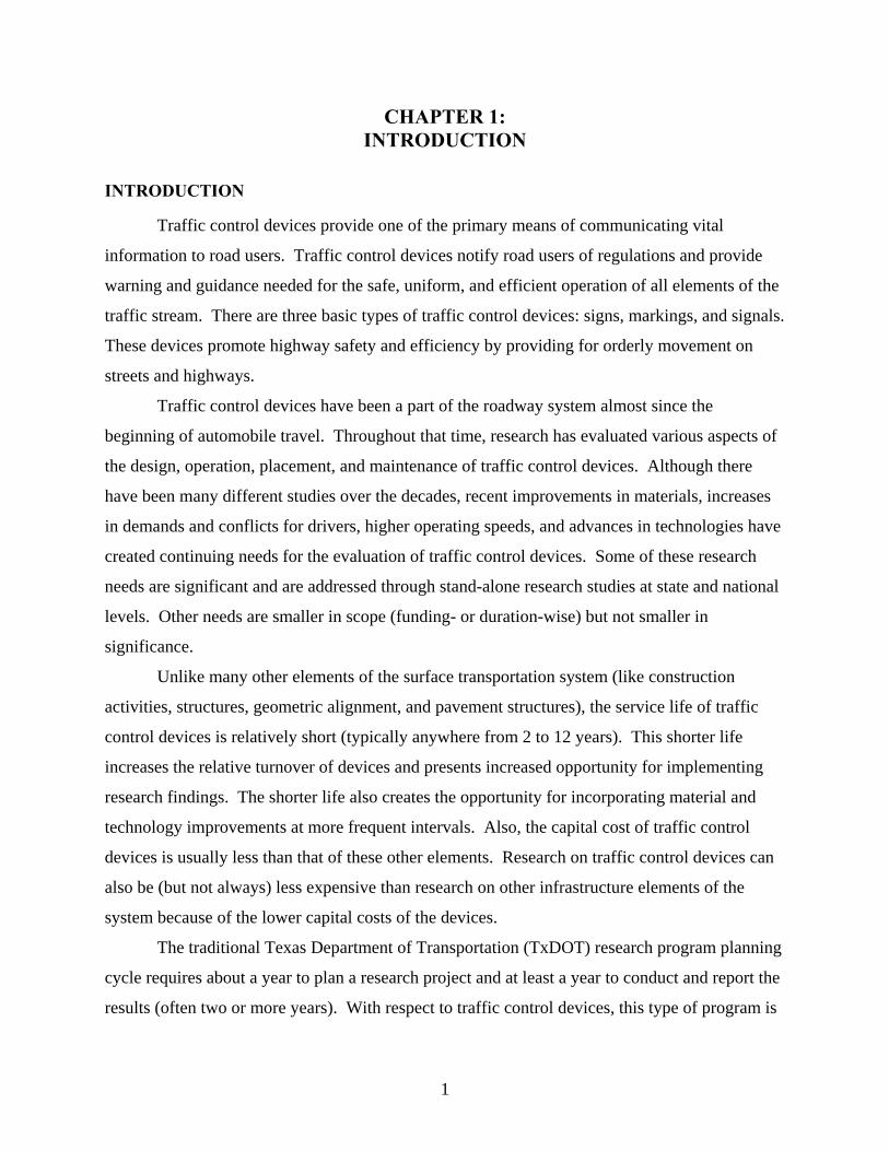
The treatment for this evaluation consisted of replacing the existing Left Turn Yield on

Green Ball sign (Figure 2-1a) with an extinguishable message sign (EMS) (Figure 2-1b). The

EMS was attached above the signal head directing the left-turn movement. The EMS was

synchronized with the signal indications. The EMS would illuminate when the yellow arrow or

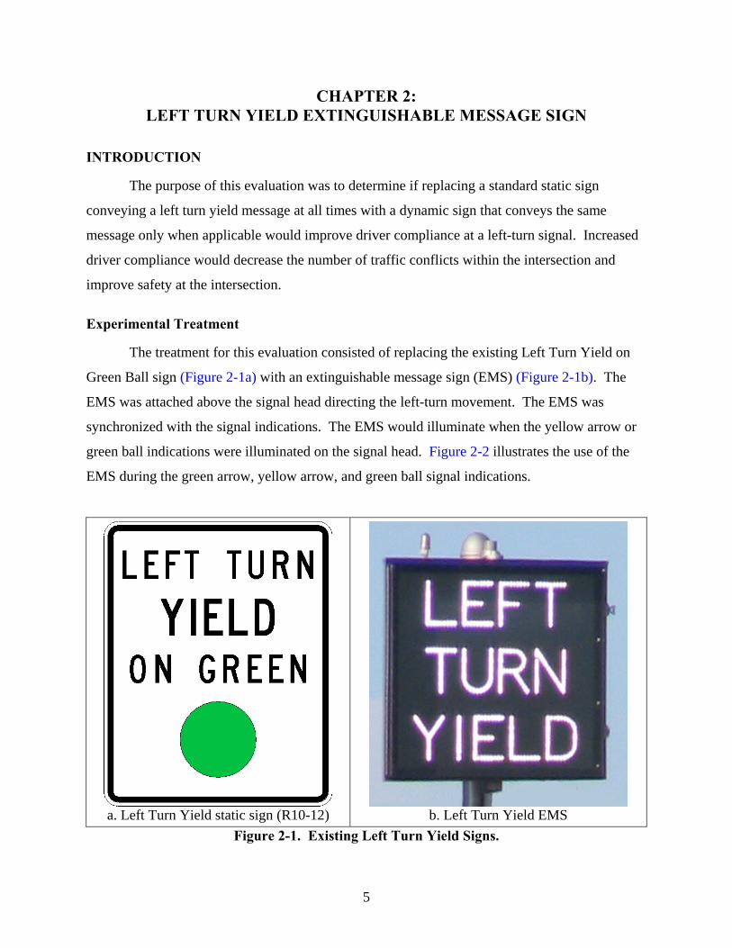
green ball indications were illuminated on the signal head. Figure 2-2 illustrates the use of the

EMS during the green arrow, yellow arrow, and green ball signal indications.

a. Left Turn Yield static sign (R10-12)

b. Left Turn Yield EMS

Figure 2-1. Existing Left Turn Yield Signs.

6

a. Protected Phase

EMS not illuminated b. End of Protected Phase

EMS illuminated c. Permitted/Permissive

EMS illuminated Figure 2-2. Operation of the Left Turn Yield EMS.

Study Objectives

The objective of the study was to determine if using an EMS with the message Left Turn

Yield would enhance the safety and reduce accidents at an intersection.

BACKGROUND INFORMATION

Various types of EMS are currently used as warning signs for weather and traffic events,

dynamic detour signing, and restriction signs for turning movements (1). An EMS is a fixed

message board (unlike a changeable message sign) that is illuminated only when required by

traffic conditions or other events. The Manual on Uniform Traffic Control Devices (MUTCD)

specifically mentions the use of EMS in railroad grade crossings and light rail transit applications

(2). Section 10C.09 reads:

“Light rail transit operations can include the use of activated blank-out sign

technology for turn prohibition (R3-1a, R3-2a) signs. The signs are typically used

on roads paralleling a semi-exclusive or mixed-use light rail transit alignment where

road users might turn across the light rail transit tracks. A blank-out sign displays its

message only when activated. When not activated, the sign face is blank.”

7

In 2001, the California Department of Transportation (CalTrans) issued a policy directive

(3) allowing the use of a left-turn yield EMS by local agencies. A field study performed by the

City of San Jose supported the policy. Between 1996 and 1999, the City of San Jose

experimented with the EMS and concluded that EMS provided a positive benefit when compared

to the existing Left Turn Yield on Green Ball sign (4). The policy statement does caution that

the San Jose study was limited in scope and did not provide a conclusive safety or operational

benefit.

The San Jose study evaluated a left-turn yield EMS against the standard MUTCD R10-12

sign and a no-sign option. The signs were installed at two intersections. One intersection had

protected/permitted phasing while the other had permitted/protected phasing. The study

addressed two questions:

• Which sign best conveyed the meaning that a driver should yield to oncoming

traffic during the green ball indication and wait for oncoming traffic to clear before

turning left?

• Did the proposed illuminated sign lead to more confusion, during the protected

phase, than the R10-12 sign or the no-sign option?

Surveys were conducted to determine driver preference given the correct meaning of each

sign and driver interpretation of the various signal indication and sign combinations. A field

study was also conducted to measure driver reaction at the study intersections. A crash history

analysis was also performed. The researchers found that drivers understood the meaning of each

sign equally. There was confusion with the use of the R10-12 sign during the protected

indication. In addition, drivers preferred the EMS when given the sign’s meaning. The crash

history analyses showed that crash rates and types do not change when using the EMS.

FIELD EVALUATION

The field evaluation was a before and after study of traffic conflicts and traffic events

within the intersection. Based on a review of previous studies and the needs of the evaluation,

the conflict study focused on left-turn related traffic conflicts and traffic events. These conflicts

and events include:

• opposing left turn,

• left turn same direction,

8

• opposing right-turn-on-red (RTOR),

• hesitating on green arrow,

• hesitating on green ball,

• left-turn red-light violation,

• left-turn yellow violation, and

• yellow trap.

Study Site

The site chosen to study the Left Turn Yield EMS was the intersection of US 59 and

Emma Lena Way in Atlanta, Texas. US 59 is a north/south four-lane divided major arterial. The

posted speed limit is 55 mph, and the 85th percentile speed is 57 mph. Emma Lena Way is an

east/west two-lane two-way minor collector that serves a large discount store and a fast-food

restaurant on the east side of the intersection. There is no posted speed. The west side of the

intersection is an access drive to a second fast-food restaurant (Figure 2-3). The treatment was

installed for both northbound and southbound left turns.

Figure 2-3. US 59 at Emma Lena Way Looking North.

9

DATA COLLECTION PROCEDURES

To study the effectiveness of the EMS, researchers collected two types of data. In the

first effort, researchers conducted a field study where they collected conflict data at a single

location before and after the EMS was installed. In the second effort, researchers acquired

accident data for the field study site for periods before and after EMS installation.

Intersection Conflict Data

The intersection conflict analyses were performed following the procedures outlined in

the Manual of Traffic Engineering Studies (5). Sample size calculations indicated that six hours

of data collection were required. The data collection was broken into two four-hour sessions

over two days. Data were collected between the hours of 1 and 6 PM to cover a peak and non-

peak period. Intersection conflicts were collected in the before condition in late October of

2004, and the after data were collected in February 2005. Two observers were stationed at the

northeast and southwest corners of the intersection to monitor and record conflicts. The

observers specifically recorded left-turn conflicts and also monitored the overall operation of the

intersection. The intersection was also recorded using video cameras from two angles in order to

collect the northbound and southbound left turns from US 59. The video was used to make

turning movement counts and to verify the left-turn conflicts.

The conflict data were divided into traffic conflicts and traffic events. Traffic conflicts

are defined as “vehicle interactions, which may lead to crashes” while traffic events are defined

as “unusual, dangerous, or illegal non-conflict maneuvers” (6). Because the focus of this study

was on left-turning traffic, the conflict analysis was focused on the northbound and southbound

US 59 left-turning movements and the conflict points associated with those movements.

Table 2-1 lists the conflicts and events used in this study.

Table 2-1. List of Traffic Conflicts and Events. Traffic Conflicts Traffic Events

Opposing left turn Hesitate on green arrow

Left turn same direction Hesitate on green ball

Opposing right-turn-on-red Left-turn red-light violation

Left-turn yellow violation

Yellow Trap

10

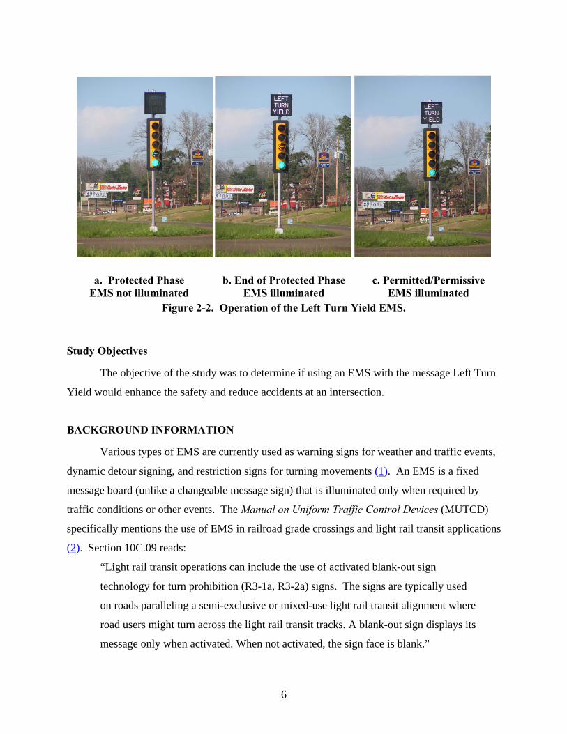
Intersection Accident Data

Accident reports from the intersection were obtained from the local police department.

The accident reports covered a period from January 2004 to June 2005. Accident data were

classified by type and location, and a condition diagram (Figure 2-4) and before and after

collision diagrams were created from the accident reports (Figures 2-5 and 2-6).

Data Reduction

Turning movement and intersection volume counts were pulled from the video data. All

volume counts were binned in 15-minute intervals. Conflict data were taken from the data

collection forms. All data were input into spreadsheets for analysis. In addition, the researchers

measured stop-bar compliance for the left-turn movements. Stop-bar compliance was also

binned into 15-minute intervals.

FIELD STUDY ANALYSIS AND RESULTS

After collecting the field data, researchers organized it into groups for analysis. After

analyzing the data, the researchers assessed the results to identify trends and assess the

effectiveness of the treatment.

Comparison of Frequency of Intersection Measures of Effectiveness

To assess whether there were any differences in the before and after conditions,

researchers compared the before and after frequencies for turning movements, traffic conflicts,

traffic events, and stop line violations. These comparisons indicated whether there was a

statistical difference in the frequency of events.

The first step in the analysis was to determine if the before and after traffic volumes were

consistent with each other. The turning movement volumes taken from the video were analyzed

using a two sample t-test. The analysis was performed in Excel using the StatistiXL add-in. The

results of the analysis are shown in Table 2-2. The before and after movement volumes are

provided, and the calculated P-value is given. At a 95 percent confidence interval (α=0.05), the

test shows that the before and after volumes are equal for all movements except the northbound

left-turn movement. In this movement, the volume decreased by approximately 32 percent. The

similarities in traffic volumes allowed for the direct comparison of the before and after results.

11

Figure 2-4. Condition Diagram Site 1: US 59 and Emma Lena Way.

Figure 2-5. Before Condition Collision Diagram.

12

Figure 2-6. After Condition Collision Diagram.

Table 2-2. Statistical Testing Results: Turning Movement Volumes. Number of Vehicles

Movement Before After Difference

P-value Counts Equal at α = 0.05?

Through 2727 2261 -466 0.238 Yes Left 982 669 -313 0.025 No

Right 158 168 10 0.528 Yes Northbound

U-turn 61 84 23 0.344 Yes Through 2517 3172 655 0.291 Yes

Left 73 129 56 0.051 Yes Right 764 959 195 0.294 Yes

Southbound

U-turn 4 22 18 0.323 Yes

13

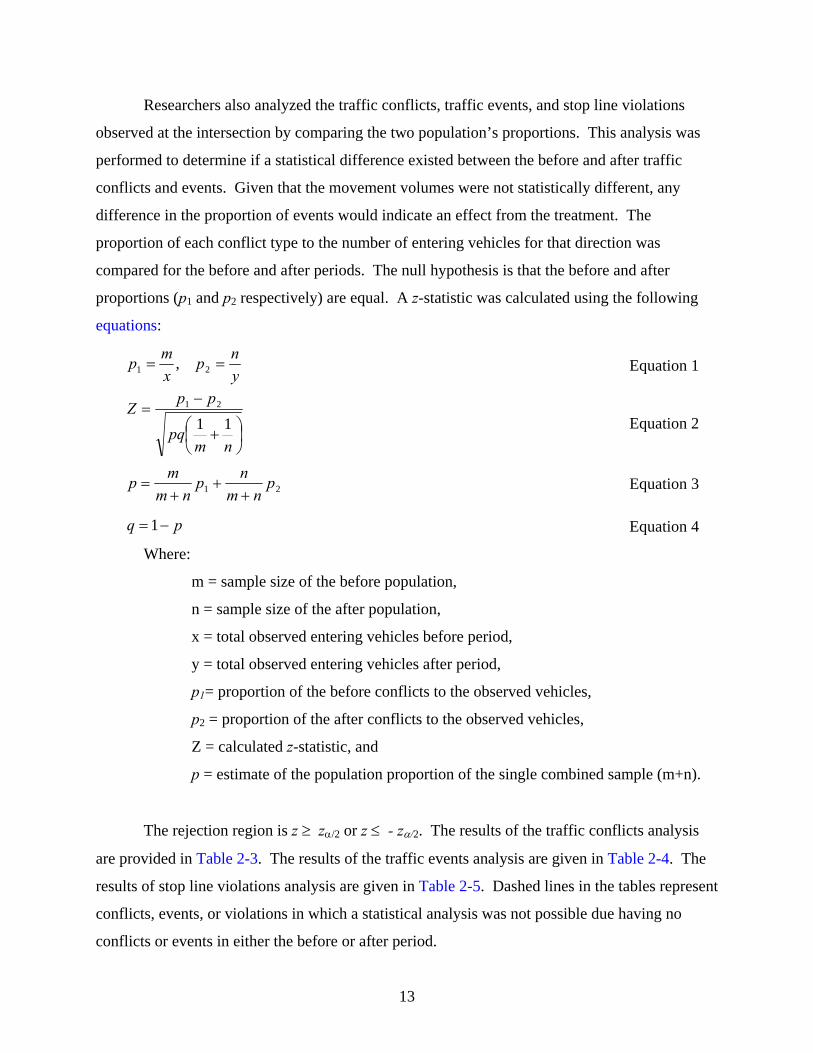
Researchers also analyzed the traffic conflicts, traffic events, and stop line violations

observed at the intersection by comparing the two population’s proportions. This analysis was

performed to determine if a statistical difference existed between the before and after traffic

conflicts and events. Given that the movement volumes were not statistically different, any

difference in the proportion of events would indicate an effect from the treatment. The

proportion of each conflict type to the number of entering vehicles for that direction was

compared for the before and after periods. The null hypothesis is that the before and after

proportions (p1 and p2 respectively) are equal. A z-statistic was calculated using the following

equations:

ynp

xmp == 21 , Equation 1

⎟⎠⎞

⎜⎝⎛ +

−=

nmpq

ppZ11

21 Equation 2

21 pnm

npnm

mp+

++

= Equation 3

pq −= 1 Equation 4

Where:

m = sample size of the before population,

n = sample size of the after population,

x = total observed entering vehicles before period,

y = total observed entering vehicles after period,

p1= proportion of the before conflicts to the observed vehicles,

p2 = proportion of the after conflicts to the observed vehicles,

Z = calculated z-statistic, and

p = estimate of the population proportion of the single combined sample (m+n).

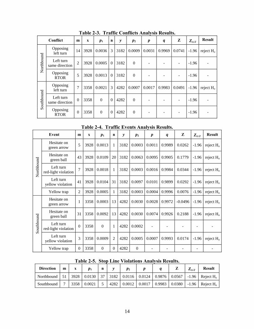
The rejection region is z ≥ zα/2 or z ≤ - zα/2. The results of the traffic conflicts analysis

are provided in Table 2-3. The results of the traffic events analysis are given in Table 2-4. The

results of stop line violations analysis are given in Table 2-5. Dashed lines in the tables represent

conflicts, events, or violations in which a statistical analysis was not possible due having no

conflicts or events in either the before or after period.

14

Table 2-3. Traffic Conflicts Analysis Results. Conflict m x p1 n y p2 p q Z Zα/2 Result

Opposing left turn 14 3928 0.0036 3 3182 0.0009 0.0031 0.9969 0.0741 -1.96 reject Ho

Left turn same direction 2 3928 0.0005 0 3182 0 - - - -1.96 -

Nor

thbo

und

Opposing RTOR 5 3928 0.0013 0 3182 0 - - - -1.96 -

Opposing left turn 7 3358 0.0021 3 4282 0.0007 0.0017 0.9983 0.0491 -1.96 reject Ho

Left turn same direction 0 3358 0 0 4282 0 - - - -1.96 -

Sout

hbou

nd

Opposing RTOR 0 3358 0 0 4282 0 - - - -1.96 -

Table 2-4. Traffic Events Analysis Results.

Event m x p1 n y p2 p q Z Zα/2 Result

Hesitate on green arrow 5 3928 0.0013 1 3182 0.0003 0.0011 0.9989 0.0262 -1.96 reject Ho

Hesitate on green ball 43 3928 0.0109 20 3182 0.0063 0.0095 0.9905 0.1779 -1.96 reject Ho

Left turn red-light violation 7 3928 0.0018 1 3182 0.0003 0.0016 0.9984 0.0344 -1.96 reject Ho

Left turn yellow violation 41 3928 0.0104 31 3182 0.0097 0.0101 0.9899 0.0292 -1.96 reject Ho

Nor

thbo

und

Yellow trap 2 3928 0.0005 1 3182 0.0003 0.0004 0.9996 0.0076 -1.96 reject Ho

Hesitate on green arrow 1 3358 0.0003 13 4282 0.0030 0.0028 0.9972 -0.0496 -1.96 reject Ho

Hesitate on green ball 31 3358 0.0092 13 4282 0.0030 0.0074 0.9926 0.2188 -1.96 reject Ho

Left turn red-light violation 0 3358 0 1 4282 0.0002 - - - - -

Left turn yellow violation 3 3358 0.0009 2 4282 0.0005 0.0007 0.9993 0.0174 -1.96 reject Ho

Sout

hbou

nd

Yellow trap 0 3358 0 0 4282 0 - - - - -

Table 2-5. Stop Line Violations Analysis Results.

Direction m x p1 n y p2 p q Z Zα/2 Result

Northbound 51 3928 0.0130 37 3182 0.0116 0.0124 0.9876 0.0567 -1.96 Reject Ho

Southbound 7 3358 0.0021 5 4282 0.0012 0.0017 0.9983 0.0380 -1.96 Reject Ho

15

The results of the analysis indicate that there is a statistically significant difference

between the before and after conditions for all measures where there was at least one event each

in both the before and after periods.

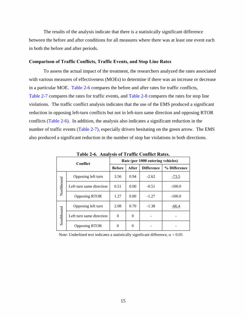
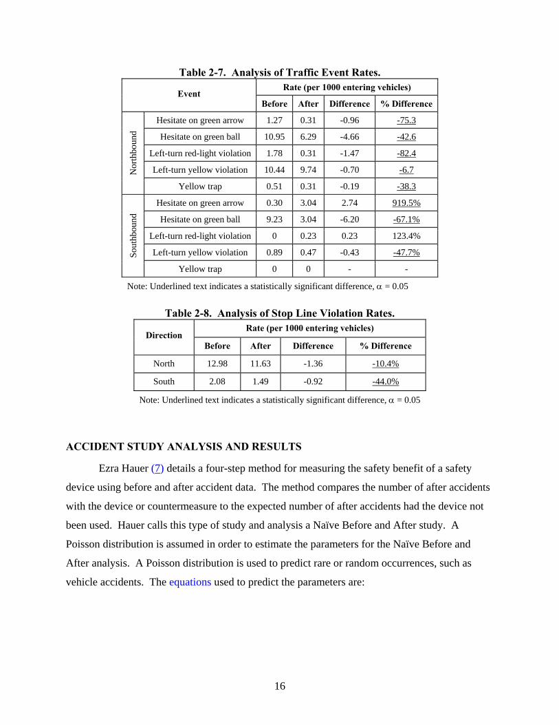
Comparison of Traffic Conflicts, Traffic Events, and Stop Line Rates

To assess the actual impact of the treatment, the researchers analyzed the rates associated

with various measures of effectiveness (MOEs) to determine if there was an increase or decrease

in a particular MOE. Table 2-6 compares the before and after rates for traffic conflicts,

Table 2-7 compares the rates for traffic events, and Table 2-8 compares the rates for stop line

violations. The traffic conflict analysis indicates that the use of the EMS produced a significant

reduction in opposing left-turn conflicts but not in left-turn same direction and opposing RTOR

conflicts (Table 2-6). In addition, the analysis also indicates a significant reduction in the

number of traffic events (Table 2-7), especially drivers hesitating on the green arrow. The EMS

also produced a significant reduction in the number of stop bar violations in both directions.

Table 2-6. Analysis of Traffic Conflict Rates. Rate (per 1000 entering vehicles)

Conflict Before After Difference % Difference

Opposing left turn 3.56 0.94 -2.62 -73.5

Left turn same direction 0.51 0.00 -0.51 -100.0

Nor

thbo

und

Opposing RTOR 1.27 0.00 -1.27 -100.0

Opposing left turn 2.08 0.70 -1.38 -66.4

Left turn same direction 0 0 - -

Sout

hbou

nd

Opposing RTOR 0 0 - -

Note: Underlined text indicates a statistically significant difference, α = 0.05

16

Table 2-7. Analysis of Traffic Event Rates. Rate (per 1000 entering vehicles)

Event Before After Difference % Difference

Hesitate on green arrow 1.27 0.31 -0.96 -75.3

Hesitate on green ball 10.95 6.29 -4.66 -42.6

Left-turn red-light violation 1.78 0.31 -1.47 -82.4

Left-turn yellow violation 10.44 9.74 -0.70 -6.7 Nor

thbo

und

Yellow trap 0.51 0.31 -0.19 -38.3

Hesitate on green arrow 0.30 3.04 2.74 919.5%

Hesitate on green ball 9.23 3.04 -6.20 -67.1%

Left-turn red-light violation 0 0.23 0.23 123.4%

Left-turn yellow violation 0.89 0.47 -0.43 -47.7% Sout

hbou

nd

Yellow trap 0 0 - -


Table 2-8. Analysis of Stop Line Violation Rates. Rate (per 1000 entering vehicles)

Direction Before After Difference % Difference

North 12.98 11.63 -1.36 -10.4%

South 2.08 1.49 -0.92 -44.0%


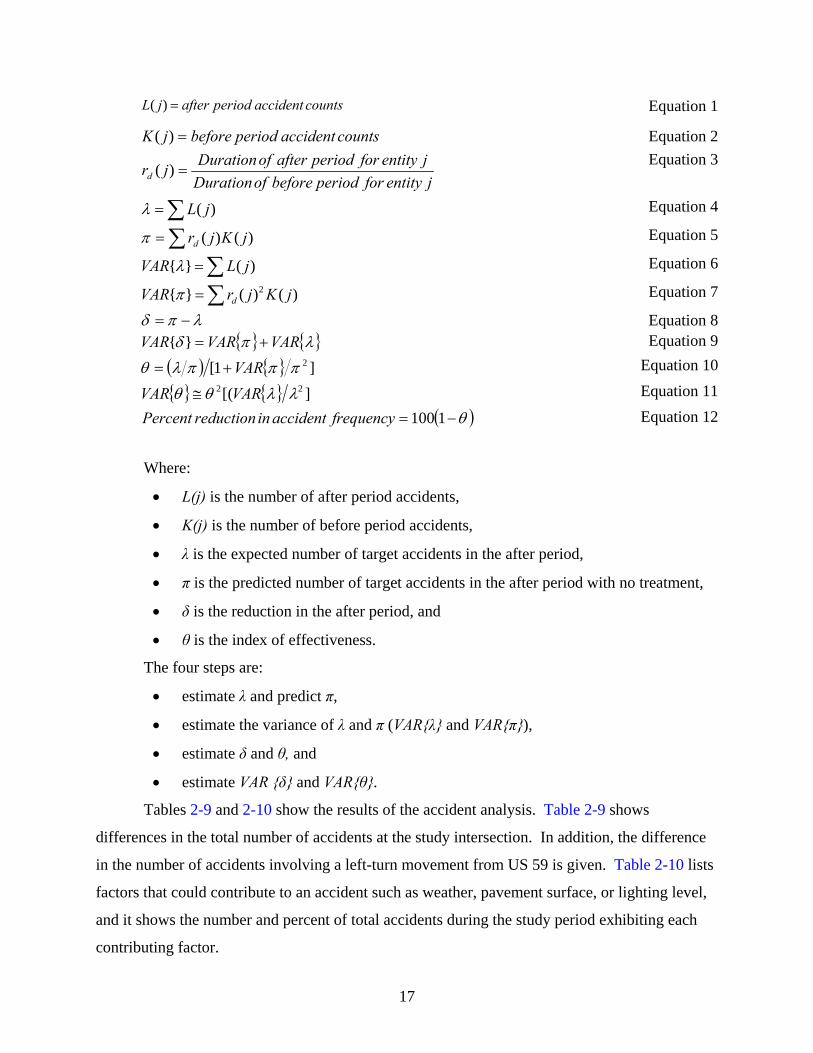
ACCIDENT STUDY ANALYSIS AND RESULTS

Ezra Hauer (7) details a four-step method for measuring the safety benefit of a safety

device using before and after accident data. The method compares the number of after accidents

with the device or countermeasure to the expected number of after accidents had the device not

been used. Hauer calls this type of study and analysis a Naïve Before and After study. A

Poisson distribution is assumed in order to estimate the parameters for the Naïve Before and

After analysis. A Poisson distribution is used to predict rare or random occurrences, such as

vehicle accidents. The equations used to predict the parameters are:

17

countsaccidentperiodafterjL =)( Equation 1

countsaccidentperiodbeforejK =)( Equation 2

jentityforperiodbeforeofDurationjentityforperiodafterofDurationjrd =)(

Equation 3

∑= )( jLλ Equation 4

∑= )()( jKjrdπ Equation 5

{ } ( )VAR L jλ =∑ Equation 62{ } ( ) ( )dVAR r j K jπ =∑ Equation 7

λπδ −= Equation 8{ } { }λπδ VARVARVAR +=}{ Equation 9

( ) { } ]1[ 2πππλθ VAR+= Equation 10

{ } { } ]([ 22 λλθθ VARVAR ≅ Equation 11

( )θ−= 1100frequencyaccidentinreductionPercent Equation 12

Where:

• L(j) is the number of after period accidents,

• K(j) is the number of before period accidents,

• λ is the expected number of target accidents in the after period,

• π is the predicted number of target accidents in the after period with no treatment,

• δ is the reduction in the after period, and

• θ is the index of effectiveness.

The four steps are:

• estimate λ and predict π,

• estimate the variance of λ and π (VAR{λ} and VAR{π}),

• estimate δ and θ, and

• estimate VAR {δ} and VAR{θ}.

Tables 2-9 and 2-10 show the results of the accident analysis. Table 2-9 shows

differences in the total number of accidents at the study intersection. In addition, the difference

in the number of accidents involving a left-turn movement from US 59 is given. Table 2-10 lists

factors that could contribute to an accident such as weather, pavement surface, or lighting level,

and it shows the number and percent of total accidents during the study period exhibiting each

contributing factor.

18

Table 2-9. Changes in Number and Type of Accidents. Category Before After Decrease % Difference

Total Number of Accidents 28 15 13 -46

Type of Collision

Right Angle 25 11 14 -56

Rear End 3 3 0 0

Single Vehicle 0 1 -1 -

Movements from US 59

NB Left Turn 8 3 5 -63

SB Left Turn 11 3 8 -73

NB Right Turn 1 3 -2 200

SB Right Turn 2 3 -1 50

Table 2-10. Accident Factors.

Before After Factors

N % N %

Lighting:

Daylight 25 89 11 73

Dusk 1 4 1 7

Dark, lighted 2 7 2 13

Pavement Surface:

Dry 24 86 11 73

Wet 4 14 4 27

Weather:

Clear 25 89 11 73

Rain 1 4 4 27

N = Number of accidents, % = Percent of total accidents during study period

Tables 2-11 and 2-12 show the analysis following Hauer’s method. The analysis is

performed for:

• all accidents,

• all left-turn accidents, and

• northbound and southbound left-turn accidents.

19

Table 2-11. Estimated Accident Reductions in the After Period. Time Period

(Months) Target Accident

Before After

Acc. Before

Acc. After rd(j) π VAR {π} δ VAR {δ}

All Accidents 10 8 28 15 0.8 22.4 17.92 7.4 32.92

Left Turn 10 8 19 6 0.8 15.2 12.16 9.2 18.16

Northbound 10 8 8 3 0.8 6.4 5.12 3.4 8.12

Southbound 10 8 11 3 0.8 8.8 7.04 5.8 10.04

Table 2-12. Estimate of the Index of Effectiveness.

Target Accident θ VAR {θ} Percent Reduction in Accident Frequency

All Accidents 0.694 0.046 30.6

Left Turn 0.416 0.034 58.4

Northbound 0.527 0.101 47.3

Southbound 0.372 0.049 62.8

SUMMARY AND CONCLUSIONS

The analysis shows that installation of a left-turn yield EMS significantly lowered the

rate of opposing left-turn traffic conflicts. The rate dropped approximately 66 percent for

southbound traffic and 74 percent for northbound traffic.

The results for traffic events are more mixed. The northbound left-turn movement had

significant reductions in the number of left-turn red-light violations and the incidence of yellow

trap events while the southbound left-turn movement had significant reductions in yellow light

violation. The southbound direction also saw a significant increase in the incidence of left-turn

red-light violations. This result is misleading, however, because the number of left-turn red-light

violations in the after condition totaled one vehicle.

The accident analysis shows an overall reduction in the number of accidents at the

intersection. The total number of accidents dropped by half. Of the three types of collisions that

occurred at the intersection, the majority were right-angle collisions. This type of collision was

also the source of all the reduction. Breaking down the right-angle collisions into the northbound

and southbound turn movements, the analysis shows that the reduction in accidents came solely

from the left-turn movements from US 59. The northbound and southbound movements had

reductions of 63 percent and 73 percent, respectively. The statistical accident analysis indicates

20

a reduction in accident frequency up to 58 percent for the left-turn movement with a 31 percent

reduction in all accidents at the intersection. Based on the results, the use of the Left Turn Yield

EMS has had a positive effect on the safety of the intersection.

RECOMMENDATIONS

The results indicate a positive safety benefit to the use of an EMS in place of the standard

Left Turn Yield on Green Ball sign. Based on the findings for this evaluation, the researchers

recommend using this type of sign at locations with a demonstrated history of high left-turn

crashes. The Texas Manual on Uniform Traffic Control Devices does not need to be revised to

accommodate this sign, but the Texas Department of Transportation may want to develop a

standard sheet or other guidelines to assist in the implementation of the device. Because these

results reflect the impact at only one intersection, additional installations of this treatment should

be monitored after installation to confirm the benefit of installation.

REFERENCES

1. Intelligent Transportation Systems (ITS) Design Manual. Wisconsin Department of

Transportation, January 2001. http://www.uwm.edu/Dept/CUTS/itsdm/. Accessed

August 10, 2005.

2. Manual on Uniform Traffic Control Devices. Federal Highway Administration,

Washington, D.C., 2003.

3. Policy Directive 01-03, Left-Turn Extinguishable Message Sign, State of California,

Department of Transportation, 2001. http://www.dot.ca.gov/hq/traffops/signtech/

signdel/policy/ 01-03.pdf. Accessed August 10, 2005.

4. Botha, J.L., J.M. Waller, J.O. Rodriguez, and R.L. Northhouse. An Illuminated Sign as a

Substitute for the MUTCD R10-10/12 Sign, Compendium of Papers. Institute of

Transportation Engineers 2000 District 6 Annual Meeting, San Diego, California, June

2000.

5. Robertson, H.D., J.E. Hummer, and D.C. Nelson. Manual of Traffic Engineering Studies.

Institute of Transportation Engineers, Prentice Hall, Englewood Cliffs, NJ, 1994, pp.

219-235.

http://www.uwm.edu/Dept/CUTS/itsdm/

http://www.dot.ca.gov/hq/traffops/signtech/ signdel/policy/ 01-03.pdf

http://www.dot.ca.gov/hq/traffops/signtech/ signdel/policy/ 01-03.pdf

21

6. Kittleson & Associates, Inc., and Texas Transportation Institute. Traffic Conflict Studies

Report Working Paper 5. National Cooperative Highway Research Program Project 3-54,

Washington, D.C., August 1999.

7. Hauer, Ezra. Observational Before-After Studies in Road Safety. Pergamon, Elsevier

Science, Inc., Tarrytown, NY, 1997.

23

CHAPTER 3: RED BORDER SPEED LIMIT SIGN

INTRODUCTION

Speed Limit signs on our highways are installed to guide and induce motorists to drive at

safe speeds. Speeding is a common occurrence on our highways and contributes to a large

number of fatal and non-fatal crashes every year. In 2003, speeding was a contributing factor in

31 percent of all fatal crashes. The National Highway Traffic Safety Administration (NHTSA)

defines speeding as driving too fast for conditions or exceeding the posted speed limit. Speed-

related crashes on Texas highways account for 41 percent of all fatal crashes (1). For these

reasons, improving speed limit compliance is a priority. Researchers hypothesized that

sometimes motorists do not comply with speed limits because Speed Limit signs do not attract

attention. This lack of compliance can be especially true in reduced speed zones well outside the

city limits of a rural community that provide no clue to the motorists for a decrease in speed limit

other than the Speed Limit sign.

In the second year of this project, the researchers expanded upon the first year effort to

evaluate the impact of using a red border Speed Limit sign on compliance with the speed limit

(2). The researchers improved upon the design of the red border sign, added sheeting type as a

factor in the evaluation, evaluated the sign at several locations, and conducted a long-term

follow-up evaluation of the red border signs installed during the first year of the project.

Experimental Treatment

The researchers believe that increasing conspicuity of the Speed Limit sign would result

in increased awareness of the posted speed limit and therefore improve compliance with the

speed limit. This study was completed using three Speed Limit sign designs:

• The standard Speed Limit sign (R2-1) (shown in Figure 3-1a). This is the standard

sign described in the Manual on Uniform Traffic Control Devices (MUTCD).

• A standard Speed Limit sign with red border added (shown in Figure 3-1b). This is

the sign that was evaluated in the first year of the project.

• A modified red border Speed Limit sign (shown in Figure 3-1c). This is the sign

that was evaluated in the second year of the project.

24

a. Standard Speed Limit Sign (R2-1) b. Standard Speed Limit Sign

with Red Border c. Modified Speed Limit

Sign Figure 3-1. Signs Evaluated.

The standard sign with a red border was created by placing a red sign that was 6 inches

wider and 6 inches taller behind the standard sign. This added a 3-inch red border around the

standard sign. The modified sign was created by replacing the black border of the standard

Speed Limit sign with a wider red border and increasing the overall sign size by 6 inches in

width and height. This allowed the red border to be 4 inches wide. The change to the 4-inch

border was based on observations of field installations of the standard sign with a red border.

Those observations indicated that the thin black border reduced the conspicuity impacts of the

red border when viewed at long distances.

Study Objectives

The basic goal of this activity was to determine if replacing the black border on a Speed

Limit sign with a wide red border would improve driver compliance with the speed limit. As

mentioned, the effort is a continuation of the previous Texas Transportation Institute (TTI) effort

during the first year of this project (2). There were two specific objectives associated with the

activity goal:

• Evaluate the short-term impacts of the modified red border Speed Limit sign at four

sites.

• Evaluate the long-term impacts (9 to 12 months after installation) of the standard

Speed Limit sign with a red border at the three sites evaluated during the first year

of the project.

25

BACKGROUND INFORMATION

Over the years, a variety of Speed Limit sign treatments and related other treatments have

been used to encourage greater compliance with speed limits. A few of these using the Reduced

Speed Ahead sign, using larger signs, attaching orange flags to the Speed Limit sign, adding a

color plaque at the top of a Speed Limit sign as a conspicuity treatment, locating the Speed Limit

sign overhead, and using speed feedback signs. The following paragraphs describe some of the

research that has been conducted on the effectiveness of a few of these treatments.

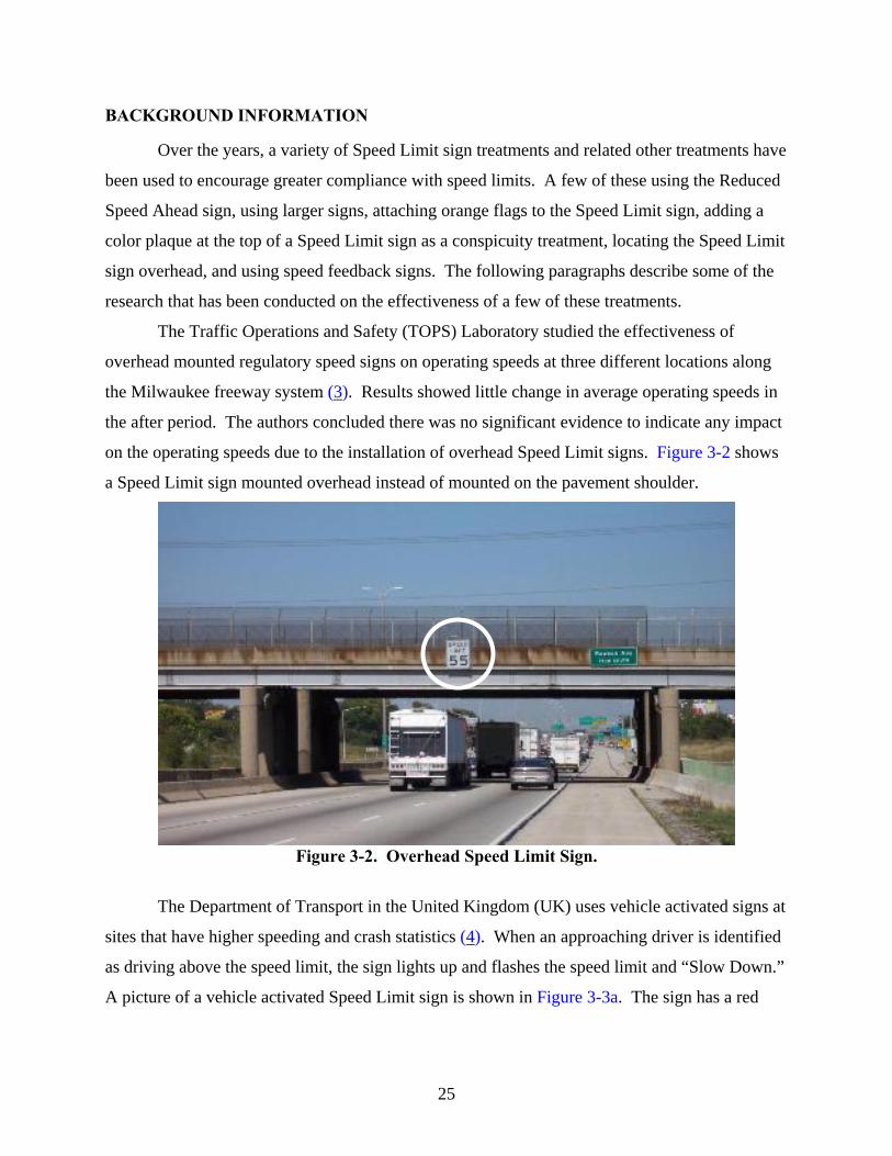
The Traffic Operations and Safety (TOPS) Laboratory studied the effectiveness of

overhead mounted regulatory speed signs on operating speeds at three different locations along

the Milwaukee freeway system (3). Results showed little change in average operating speeds in

the after period. The authors concluded there was no significant evidence to indicate any impact

on the operating speeds due to the installation of overhead Speed Limit signs. Figure 3-2 shows

a Speed Limit sign mounted overhead instead of mounted on the pavement shoulder.

Figure 3-2. Overhead Speed Limit Sign.

The Department of Transport in the United Kingdom (UK) uses vehicle activated signs at

sites that have higher speeding and crash statistics (4). When an approaching driver is identified

as driving above the speed limit, the sign lights up and flashes the speed limit and “Slow Down.”

A picture of a vehicle activated Speed Limit sign is shown in Figure 3-3a. The sign has a red

26

circular border around the posted speed limit, which is the case for all Speed Limit signs in the

UK. Most Speed Limit signs on European highways have red borders as shown in Figure 3-3b.

a. Vehicle Activated Sign

b. International Speed Limit Sign

Note: In both signs, the circle around the speed is red. Figure 3-3. International Speed Limit Signs.

In the United States, the first known study to evaluate the use of a red border around a

Speed Limit sign was conducted by TTI in a previous research project (5). The researchers

evaluated the effect of a 3-inch red border around a standard Speed Limit sign in a rural speed

zone. The sign evaluated in that effort was the same at that shown in Figure 3-1b. The results of

this study indicated a significant decrease in the mean speeds of passenger vehicles traveling

during both daytime and nighttime. The percentage of vehicles exceeding the speed limit also

decreased from 80 percent to 65 percent—a statistically significant amount.

The initial TTI research on the red border treatment appeared beneficial, but since the

evaluation was conducted at only one site, the results needed additional evaluation to support a

wider spread application. Researchers conducted additional evaluations during the first year of

the 4701 research project (2). The first year effort found promising and beneficial results at three

of the four sites, but the findings were not conclusive enough to recommend a change in the

design of Speed Limit signs. Furthermore, observations of the first year installations indicated

that the red border treatment was not wide enough to provide the desired level of conspicuity.

27

SECOND YEAR STUDY APPROACH

This research activity was divided into a short-term study and a long-term study. In the

short-term study, researchers conducted a before and after analysis of the effectiveness of the

modified Speed Limit sign at four sites. The after evaluations were conducted within eight

weeks of the treatment installation. In the long-term study, researchers conducted a second after

study at the three sites evaluated during the first year of the project. These after evaluations

(referred to as long after evaluations) were conducted 9 to 12 months after the treatment

installation.

Short-Term Study

The short-term study evaluated the effectiveness of the modified red border Speed Limit

sign (Figure 3-1c) at four sites. These sites were different from the sites evaluated during the

first year. Three different sheeting materials were used with the standard and modified signs.

Researchers collected before and after speed data at each site using road tubes and traffic

counters.

Short-Term Study Sites

The researchers selected four sites for evaluating the treatment during the second year.

The sites were selected using criteria developed for the first year study effort (2). The primary

consideration for selection of a site was that it represented a rural condition where there was no

change in the roadway environment and no apparent reason for a change in the speed limit. The

four sites are listed below, and a more detailed description of each site is provided in the

following paragraphs:

• Site 1—SH 7 eastbound traffic approaching Marlin,

• Site 2—SH 14 southbound traffic approaching Wortham,

• Site 3—US 79 northbound traffic approaching Oakwood, and

• Site 4—FM 39 northbound traffic approaching Normangee.

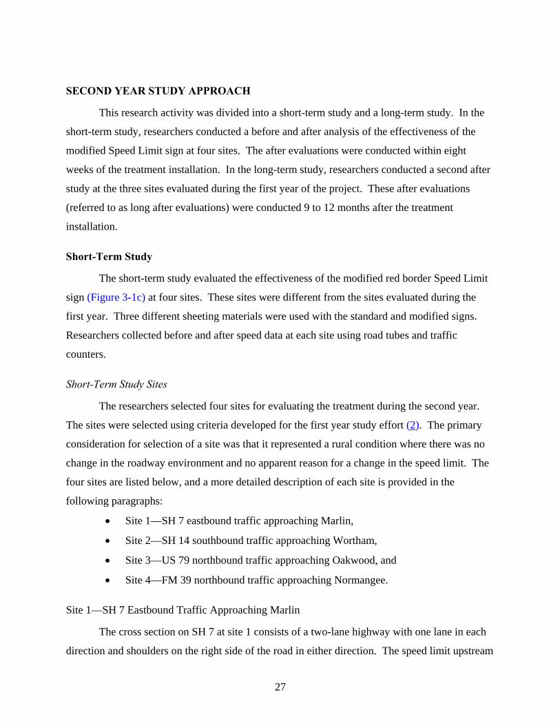
Site 1—SH 7 Eastbound Traffic Approaching Marlin

The cross section on SH 7 at site 1 consists of a two-lane highway with one lane in each

direction and shoulders on the right side of the road in either direction. The speed limit upstream

28

of the 55 mph Speed Limit sign is 70 mph. The area is rural approaching the town of Marlin.

The data at this site were collected using portable automated classifiers connected to pneumatic

tubes. The existing sign was 24×30 inches in size with high intensity sheeting. Figure 3-4 is a

photo of the site with the red border sign installed.

Figure 3-4. Site 1—SH 7, Marlin Site after Modified Red Border Treatment.

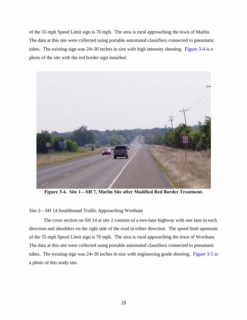
Site 2—SH 14 Southbound Traffic Approaching Wortham

The cross section on SH 14 at site 2 consists of a two-lane highway with one lane in each


of the 55 mph Speed Limit sign is 70 mph. The area is rural approaching the town of Wortham.


tubes. The existing sign was 24×30 inches in size with engineering grade sheeting. Figure 3-5 is

a photo of this study site.

29

Figure 3-5. Site 2—SH 14, Wortham Site before Modified Red Border Treatment.

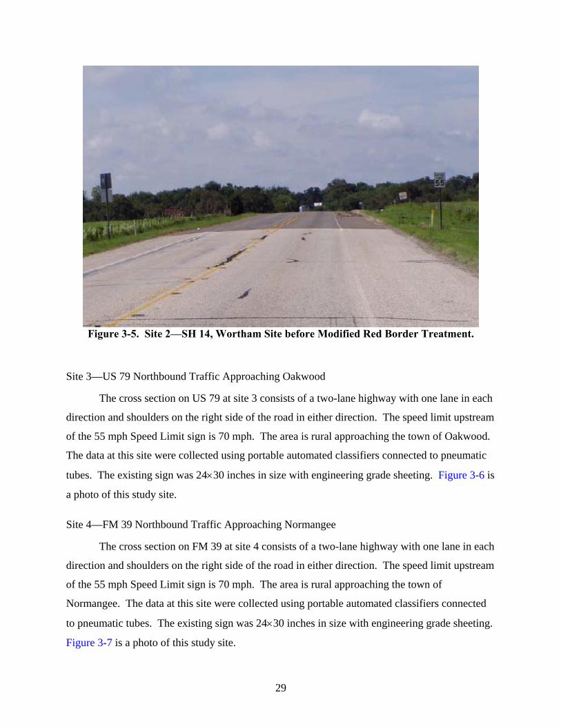
Site 3—US 79 Northbound Traffic Approaching Oakwood

The cross section on US 79 at site 3 consists of a two-lane highway with one lane in each


of the 55 mph Speed Limit sign is 70 mph. The area is rural approaching the town of Oakwood.


tubes. The existing sign was 24×30 inches in size with engineering grade sheeting. Figure 3-6 is

a photo of this study site.

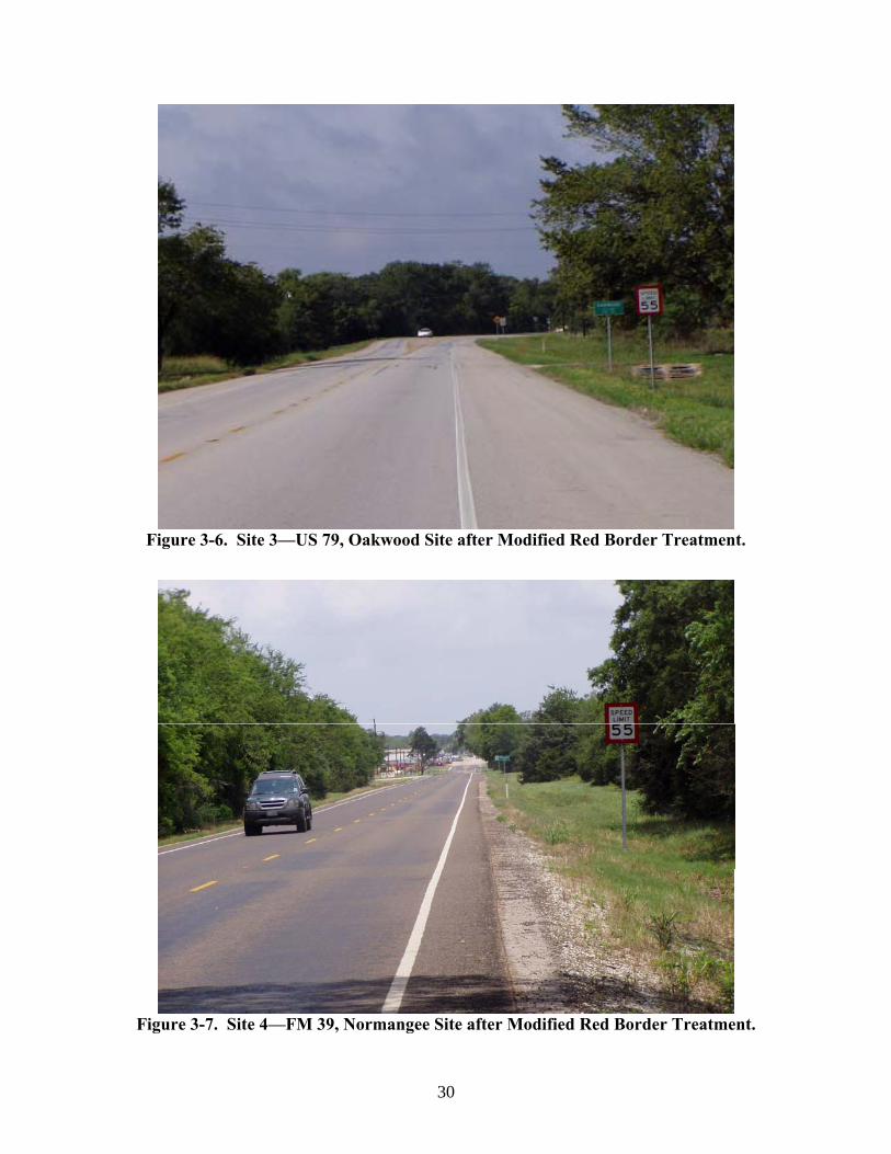
Site 4—FM 39 Northbound Traffic Approaching Normangee

The cross section on FM 39 at site 4 consists of a two-lane highway with one lane in each


of the 55 mph Speed Limit sign is 70 mph. The area is rural approaching the town of

Normangee. The data at this site were collected using portable automated classifiers connected

to pneumatic tubes. The existing sign was 24×30 inches in size with engineering grade sheeting.

Figure 3-7 is a photo of this study site.

30

Figure 3-6. Site 3—US 79, Oakwood Site after Modified Red Border Treatment.

Figure 3-7. Site 4—FM 39, Normangee Site after Modified Red Border Treatment.

31

Treatments for Short-Term Study

The treatments evaluated in the short-term study consisted of two sign designs using

various combinations of three sheeting types. This evaluation was completed at four new sites

using two sign designs and three sheeting materials. The two sign signs were the standard sign

(Figure 3-1a) and the modified sign (Figure 3-1c). Combinations of engineering grade, high

intensity, and microprismatic sheeting were used with each design as listed below. Table 3-1

shows the sign design and sheeting combinations evaluated at each site.

• standard Speed Limit sign with engineering grade (EG) sheeting, hereafter

designated as EGS;

• standard Speed Limit sign with high intensity (HI) sheeting, hereafter designated as

HIS;

• standard Speed Limit sign with microprismatic (MP) sheeting, hereafter designated

as MPS;

• modified red border Speed Limit sign with high intensity sheeting, hereafter

designated as HIR; and

• modified red border Speed Limit sign with microprismatic sheeting, hereafter

designated as MPR.

Table 3-1. Signs Evaluated at Each Site. Site

Sign SH 7 SH 14 US 79 FM 39

EGS - X X X

HIS X X - X

MPS X X X -

HIR X X - X

MPR X X X -

Researchers hypothesized that nighttime speed limit compliance will improve as the

sheeting performance increases and compliance will improve overall with the use of the red

border treatment. Figure 3-8 illustrates the progression in sheeting improvement and the red

border treatment. To understand the impact of individual signs with respect to all other signs,

32

treatments were analyzed in pairs. Pair-wise analysis also makes it possible to directly compare

the results of the before and after studies. Table 3-2 shows all of the pairs that were analyzed.

Figure 3-8. Progression of Sign Evaluations.

Table 3-2. Treatment Pairs Evaluated at each Site. Site

Treatment Type of Treatment

Treatment Pair (from - to) SH 7 SH 14 US 79 FM 39

1 Sheeting Only EGS - HIS - X - X

2 Sheeting Only EGS - MPS - X X -

3 Sheeting Only HIS - MPS X X - -

4 Sheeting and Border EGS - HIR - X - X

5 Sheeting and Border HIS - HIR X X - X

6 Sheeting and Border MPS - HIR X X - -

7 Sheeting and Border EGS - MPR - X X -

8 Sheeting and Border HIS - MPR X X - -

9 Sheeting and Border MPS - MPR X X X -

10 Sheeting Only HIR - MPR X X - -

Data Collection for Short-Term Study

For the short-term study, researchers measured speeds at three locations using three

automated vehicle classifiers. A speed trap was established at each location by using a pair of

pneumatic tubes on the pavement. Figure 3-9 shows the data collection layout. The location of

each classifier was decided based on the following factors:

• Control Point (Point 1)—This classifier was located upstream of the treatment

location such that the Speed Limit sign could not be seen at this location, thus

33

serving as a control point that allowed comparison of before and after speed data to

determine if the before and after conditions were comparable. This point was

typically located approximately a half-mile upstream of the Speed Limit sign.

• Legibility Point (Point 2)—This classifier was located at a point well within the

legibility of the speed number in the Speed Limit sign. This point represents a

location where the driver should be able to clearly read the sign. The location was

typically located approximately 250 feet from the Speed Limit sign.

• Downstream Point (Point 3)—This classifier was located approximately 500 feet

downstream of the Speed Limit sign. It represents the point at which the driver

should clearly have adjusted the vehicle speed to the lower speed limit.

Figure 3-9. Data Collection Layout for Short-Term Study.

Data were collected during weekdays, except for existing signs at two sites, and during

clear weather. If rains occurred while data collection equipment was in the field, data collected

during rain times were deleted from the final data used for analysis. Table 3-3 shows the dates

for the short-term data collection at each site.

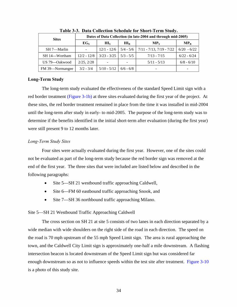
34

Table 3-3. Data Collection Schedule for Short-Term Study. Dates of Data Collection (in late-2004 and through mid-2005)

Sites EGS HIS HIR MPS MPR

SH 7—Marlin - 12/1 - 12/6 5/4 - 5/6 7/11 - 7/13, 7/19 - 7/22 6/20 - 6/22

SH 14—Wortham 12/2 - 12/8 3/23 - 3/25 5/3 - 5/5 7/13 - 7/15 6/22 - 6/24

US 79—Oakwood 2/25, 2/28 - - 5/11 - 5/13 6/8 - 6/10

FM 39—Normangee 3/2 - 3/4 5/10 - 5/12 6/6 - 6/8 - -

Long-Term Study

The long-term study evaluated the effectiveness of the standard Speed Limit sign with a

red border treatment (Figure 3-1b) at three sites evaluated during the first year of the project. At

these sites, the red border treatment remained in place from the time it was installed in mid-2004

until the long-term after study in early- to mid-2005. The purpose of the long-term study was to

determine if the benefits identified in the initial short-term after evaluation (during the first year)

were still present 9 to 12 months later.

Long-Term Study Sites

Four sites were actually evaluated during the first year. However, one of the sites could

not be evaluated as part of the long-term study because the red border sign was removed at the

end of the first year. The three sites that were included are listed below and described in the

following paragraphs:

• Site 5—SH 21 westbound traffic approaching Caldwell,

• Site 6—FM 60 eastbound traffic approaching Snook, and

• Site 7—SH 36 northbound traffic approaching Milano.

Site 5—SH 21 Westbound Traffic Approaching Caldwell

The cross section on SH 21 at site 5 consists of two lanes in each direction separated by a

wide median with wide shoulders on the right side of the road in each direction. The speed on

the road is 70 mph upstream of the 55 mph Speed Limit sign. The area is rural approaching the

town, and the Caldwell City Limit sign is approximately one-half a mile downstream. A flashing

intersection beacon is located downstream of the Speed Limit sign but was considered far

enough downstream so as not to influence speeds within the test site after treatment. Figure 3-10

is a photo of this study site.

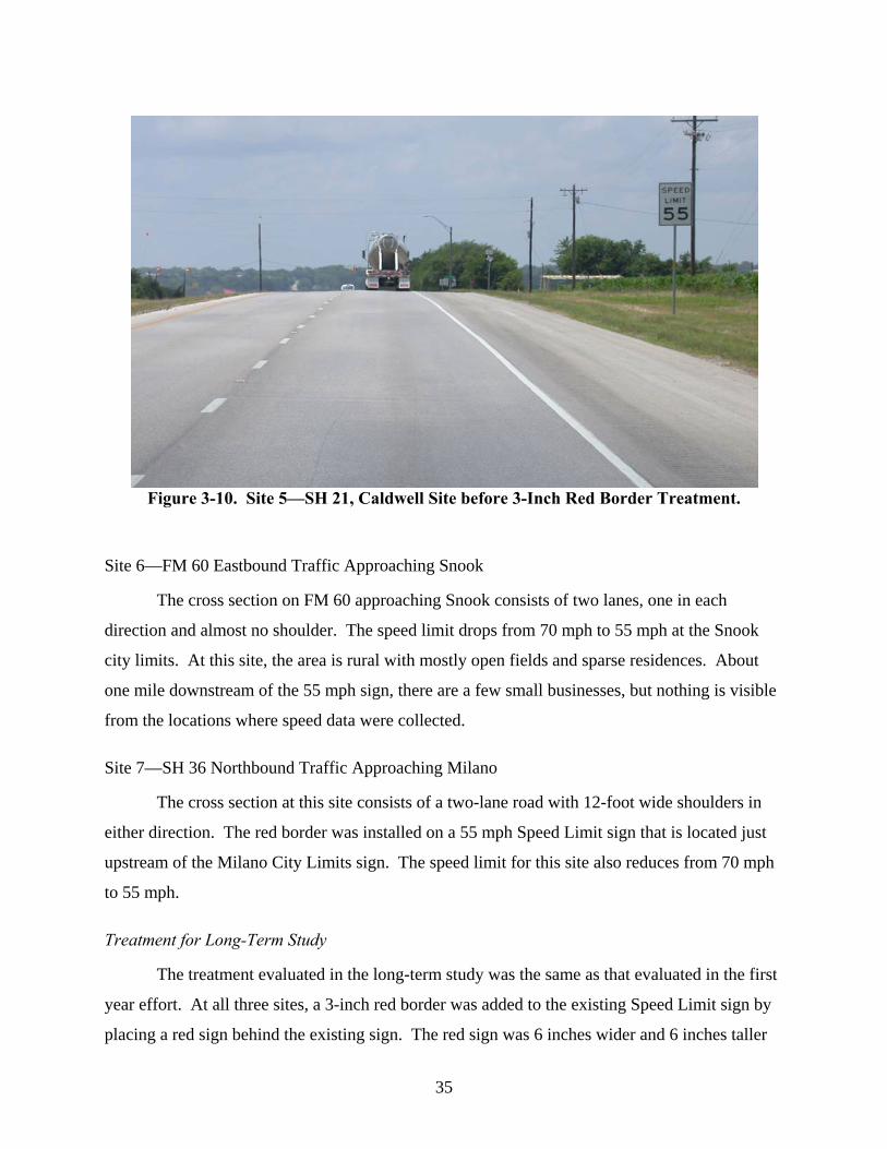
35

Figure 3-10. Site 5—SH 21, Caldwell Site before 3-Inch Red Border Treatment.

Site 6—FM 60 Eastbound Traffic Approaching Snook

The cross section on FM 60 approaching Snook consists of two lanes, one in each

direction and almost no shoulder. The speed limit drops from 70 mph to 55 mph at the Snook

city limits. At this site, the area is rural with mostly open fields and sparse residences. About

one mile downstream of the 55 mph sign, there are a few small businesses, but nothing is visible

from the locations where speed data were collected.

Site 7—SH 36 Northbound Traffic Approaching Milano

The cross section at this site consists of a two-lane road with 12-foot wide shoulders in

either direction. The red border was installed on a 55 mph Speed Limit sign that is located just

upstream of the Milano City Limits sign. The speed limit for this site also reduces from 70 mph

to 55 mph.

Treatment for Long-Term Study

The treatment evaluated in the long-term study was the same as that evaluated in the first

year effort. At all three sites, a 3-inch red border was added to the existing Speed Limit sign by

placing a red sign behind the existing sign. The red sign was 6 inches wider and 6 inches taller

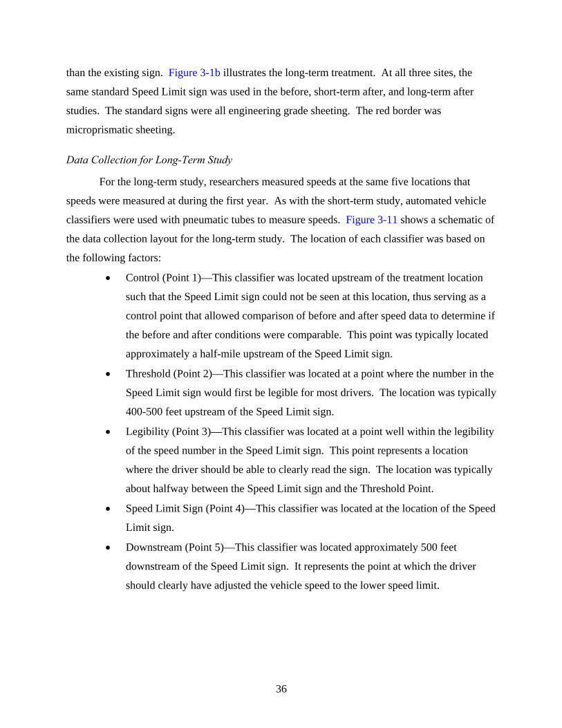
36

than the existing sign. Figure 3-1b illustrates the long-term treatment. At all three sites, the

same standard Speed Limit sign was used in the before, short-term after, and long-term after

studies. The standard signs were all engineering grade sheeting. The red border was

microprismatic sheeting.

Data Collection for Long-Term Study

For the long-term study, researchers measured speeds at the same five locations that

speeds were measured at during the first year. As with the short-term study, automated vehicle

classifiers were used with pneumatic tubes to measure speeds. Figure 3-11 shows a schematic of

the data collection layout for the long-term study. The location of each classifier was based on

the following factors:

• Control (Point 1)—This classifier was located upstream of the treatment location

such that the Speed Limit sign could not be seen at this location, thus serving as a

control point that allowed comparison of before and after speed data to determine if

the before and after conditions were comparable. This point was typically located

approximately a half-mile upstream of the Speed Limit sign.

• Threshold (Point 2)—This classifier was located at a point where the number in the

Speed Limit sign would first be legible for most drivers. The location was typically

400-500 feet upstream of the Speed Limit sign.

• Legibility (Point 3)—This classifier was located at a point well within the legibility

of the speed number in the Speed Limit sign. This point represents a location

where the driver should be able to clearly read the sign. The location was typically

about halfway between the Speed Limit sign and the Threshold Point.

• Speed Limit Sign (Point 4)—This classifier was located at the location of the Speed

Limit sign.

• Downstream (Point 5)—This classifier was located approximately 500 feet

downstream of the Speed Limit sign. It represents the point at which the driver

should clearly have adjusted the vehicle speed to the lower speed limit.

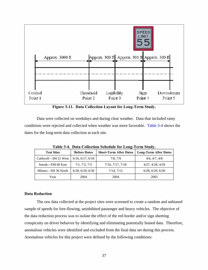
37

Figure 3-11. Data Collection Layout for Long-Term Study.

Data were collected on weekdays and during clear weather. Data that included rainy

conditions were rejected and collected when weather was more favorable. Table 3-4 shows the

dates for the long-term data collection at each site.

Table 3-4. Data Collection Schedule for Long-Term Study. Test Sites Before Dates Short-Term After Dates Long-Term After Dates

Caldwell—SH 21 West 6/16, 6/17, 6/18 7/8, 7/9 4/6, 4/7, 4/8

Snook—FM 60 East 7/1, 7/2, 7/3 7/16, 7/17, 7/18 4/27, 4/28, 4/29

Milano—SH 36 North 6/28, 6/29, 6/30 7/14, 7/15 6/28, 6/29, 6/30

Year 2004 2004 2005

Data Reduction

The raw data collected at the project sites were screened to create a random and unbiased

sample of speeds for free-flowing, uninhibited passenger and heavy vehicles. The objective of

the data reduction process was to isolate the effect of the red border and/or sign sheeting

conspicuity on driver behavior by identifying and eliminating potentially biased data. Therefore,

anomalous vehicles were identified and excluded from the final data set during this process.

Anomalous vehicles for this project were defined by the following conditions:

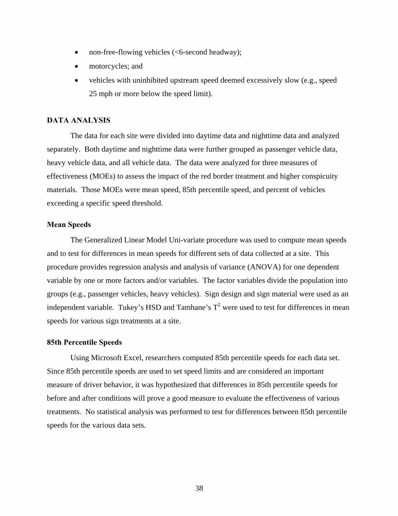
38

• non-free-flowing vehicles (<6-second headway);

• motorcycles; and

• vehicles with uninhibited upstream speed deemed excessively slow (e.g., speed

25 mph or more below the speed limit).

DATA ANALYSIS

The data for each site were divided into daytime data and nighttime data and analyzed

separately. Both daytime and nighttime data were further grouped as passenger vehicle data,

heavy vehicle data, and all vehicle data. The data were analyzed for three measures of

effectiveness (MOEs) to assess the impact of the red border treatment and higher conspicuity

materials. Those MOEs were mean speed, 85th percentile speed, and percent of vehicles

exceeding a specific speed threshold.

Mean Speeds

The Generalized Linear Model Uni-variate procedure was used to compute mean speeds

and to test for differences in mean speeds for different sets of data collected at a site. This

procedure provides regression analysis and analysis of variance (ANOVA) for one dependent

variable by one or more factors and/or variables. The factor variables divide the population into

groups (e.g., passenger vehicles, heavy vehicles). Sign design and sign material were used as an

independent variable. Tukey’s HSD and Tamhane’s T2 were used to test for differences in mean

speeds for various sign treatments at a site.

85th Percentile Speeds

Using Microsoft Excel, researchers computed 85th percentile speeds for each data set.

Since 85th percentile speeds are used to set speed limits and are considered an important

measure of driver behavior, it was hypothesized that differences in 85th percentile speeds for

before and after conditions will prove a good measure to evaluate the effectiveness of various

treatments. No statistical analysis was performed to test for differences between 85th percentile

speeds for the various data sets.

39

Percent Exceeding a Specified Speed Threshold

Microsoft Excel was used to compute the percent of vehicles exceeding a specific speed

threshold. The difference in the percent of vehicles exceeding a specific speed provides the

change in upper extremities of the data. Thus, this measure provides insight for differences in

mean speeds. For example, a decrease in average speed and decrease in percent vehicles

exceeding a threshold speed would mean faster vehicles decelerated. On the other hand, a

decrease in average speed and increase in percent vehicles exceeding a specific speed threshold

would mean slower vehicles decelerated more. No direct statistical tests were performed to test

for differences in percent vehicles exceeding the speed threshold between various sign

treatments.

RESULTS FOR SHORT-TERM STUDY

The short-term study evaluated the change in speeds at four study sites (SH 7, SH 14,

US 79, and FM 39) due to changes made to the Speed Limit sign. For the short-term study, the

impacts of the changes were measured within weeks of making the change. As indicated in

Table 3-2, there were two types of treatments in the short-term study: those treatments that

involved only a change in the sign sheeting and those treatments that included both a change in

the sheeting and replacing the black border with a wide red border. The sheeting-only treatments

were included in the study plan to provide a better assessment of the impacts of sheeting on the

effectiveness of the Speed Limit sign. Results for each type of treatment are presented in the

following pages. The short-term results presented in this chapter are supported by additional

information contained in Appendix A.

ANOVA tests were performed on mean speeds, and then post hoc tests were performed

to determine the statistical significance for difference in means for data collected at each site for

all treatments used at that site. Daytime and nighttime data were analyzed separately. Daytime

data as well as nighttime data were then analyzed for all vehicles, passenger vehicles, and heavy

vehicles. Results were then organized in pairs of sign designs and sheeting combinations

evaluated. In order to better understand the effect of experimental signs and sheeting materials,

results are presented in a before-after fashion, taking only one combination at a time.

40

Results for Sheeting-Only Treatments

The sheeting-only treatments are those treatments where the sign sheeting was changed

but there were no changes in the sign design. The impacts of these changes would be expected

to be minimal in daytime conditions and have increasing benefit in the nighttime condition as the

sign brightness increases. The specific treatments included in this type are listed below:

• Treatment #1—Change EG standard sign to HI standard sign. Treatment

implemented at two sites.

• Treatment #2—Change EG standard sign to MP standard sign. Treatment


• Treatment #3—Change HI standard sign to MP standard sign. Treatment


• Treatment #10—Change modified HI red border sign to modified MP red border

sign. Treatment implemented at two sites.

The results of the short-term data analysis for these four treatments are presented in

Appendix A in Tables A-1 through A-12 and A-37 through A-40. Table 3-5 indicates the

changes in the mean speeds for all vehicles at the control point and the downstream point and

whether the change was an increase or decrease. It also indicates whether the changes in mean

speeds from the before speed to the after conditions are statistically significant. These data give

an indication of the comparability of the before and after data at a particular site. For the

treatment to have a beneficial effect, one of three conditions would exist: the reduction at the

downstream point is greater than the reduction at the control point, the increase at the

downstream point is less than the increase at the control point, or there is a reduction at the

downstream point and an increase at the upstream point. These conditions existed at only 6 of

the 15 cases. Furthermore, the change in speeds from before to after was generally less than

1.5 mph for all of the standard sign (no red border) treatments. Based on the analysis of mean

speeds, changing the sign sheeting had little beneficial effect on speed limit compliance.

41

Table 3-5. Changes in Mean Speeds for Short-Term Study: Sheeting Only. Changes in Mean Speeds (mph)

from Before to After Appendix Table Condition Treatment Measure

SH 7 SH 14 US 79 FM 39 A-1 Daytime 1—EGS to HIS Control - -1.2* - 0.8 A-1 Daytime 1—EGS to HIS Downstream - -0.1 - 3.5* A-3 Nighttime 1—EGS to HIS Control - -1.3* - 0.5 A-3 Nighttime 1—EGS to HIS Downstream - -0.4 - 2.3* A-5 Daytime 2—EGS to MPS Control - -1.1* -0.5* - A-5 Daytime 2—EGS to MPS Downstream - -1.3* -0.7* - A-7 Nighttime 2—EGS to MPS Control - -1.1* 0.7 - A-7 Nighttime 2—EGS to MPS Downstream - -0.4 -0.1 - A-9 Daytime 3—HIS to MPS Control 1.9* 0.1 - - A-9 Daytime 3—HIS to MPS Downstream -0.4 -1.2* - -

A-11 Nighttime 3—HIS to MPS Control - 0.2 - - A-11 Nighttime 3—HIS to MPS Downstream - 0.0 - - A-37 Daytime 10—HIR to MPR Control -3.4* -3.0* - - A-37 Daytime 10—HIR to MPR Downstream 0.5 0.9* - - A-39 Nighttime 10—HIR to MPR Control -2.9* -3.1* - - A-39 Nighttime 10—HIR to MPR Downstream 0.2 -0.2 - -

Note: Asterisk (*) indicates a statistically significant difference between the before and after speed.

Table 3-6 summarizes the changes between the before and after 85th percentile speed for

all vehicles at the control and downstream points. As speed limits are based on 85th percentile

speeds, these data provide a useful assessment of the impact of the treatment on changes in speed

limit compliance. As with the mean speeds, for the treatment to have a beneficial effect, the

relationship between control and downstream points would have to be the same. The 85th

percentile speed data showed trends similar to the mean speeds, with six conditions indicating a

beneficial effect and nine that did not. Based on the analysis of 85th percentile speeds, changing

the sign sheeting had little beneficial effect on speed limit compliance.

The findings for the sheeting-only treatments indicate that there were no consistent trends

in the impacts of the sheeting change in daytime or nighttime conditions. For all combinations,

the changes in speeds at all sites were small and included both increases and decreases. Based

on these results, the impacts of changing the sheeting on a standard or modified Speed Limit sign

on driver compliance with the speed limit is minimal or nonexistent.

42

Table 3-6. Changes in 85th Percentile Speeds for Short-Term Study: Sheeting Only. Change in 85th Percentile Speed (mph)

from Before to After Appendix Table Condition Treatment Location

SH 7 SH 14 US 79 FM 39

A-1 Day 1—EGS to HIS Control - -0.9 - 1.5

A-1 Day 1—EGS to HIS Downstream - -0.4 - 5.0

A-3 Night 1—EGS to HIS Control - -1.3 - 2.0

A-3 Night 1—EGS to HIS Downstream - -1.0 - 3.0

A-5 Day 2—EGS to MPS Control - -0.5 0.0 -

A-5 Day 2—EGS to MPS Downstream - -1.1 0.0 -

A-7 Night 2—EGS to MPS Control - -0.9 1.0 -

A-7 Night 2—EGS to MPS Downstream - -2.2 0.0 -

A-9 Day 3—HIS to MPS Control 2.5 0.4 - -

A-9 Day 3—HIS to MPS Downstream -0.4 -0.7 - -

A-11 Night 3—HIS to MPS Control - 0.4 - -

A-11 Night 3—HIS to MPS Downstream - -1.2 - -

A-37 Day 10—HIR to MPR Control -3.6 -3.7 - -

A-37 Day 10—HIR to MPR Downstream 0.9 0.4 - -

A-39 Night 10—HIR to MPR Control -2.9 -4.3 - -

A-39 Night 10—HIR to MPR Downstream 0.0 -1.3 - -

Results for Border and Sheeting Treatments

The border and sheeting treatments are those treatments where the sign design was

modified to incorporate the wide red border. The modified red border sign design was evaluated

with various types of sign sheeting. The impacts of the sign design were expected to be apparent

in both daytime and nighttime conditions, while the impact of the sheeting was expected to be

minimal in daytime but more pronounced during nighttime. The specific treatments included in

this type are listed below:

• Treatment #4—Change EG standard sign to modified red border HI sign.

Treatment implemented at two sites.

• Treatment #5—Change HI standard sign to modified red border HI sign.

Treatment implemented at three sites.

• Treatment #6—Change MP standard sign to modified red border HI sign.


43

• Treatment #7—Change EG standard sign to modified red border MP sign.


• Treatment #8—Change HI standard sign to modified red border MP sign.


• Treatment #9—Change MP standard sign to modified red border MP sign.


For the analysis of the sign redesign, the researchers evaluated the data relative to mean

speeds, 85th percentile speeds, percent of vehicles exceeding speed thresholds, and the change in

speeds between the control and downstream points. The results of the short-term data analysis

for the red border and sheeting treatments are presented in Appendix A in Tables A-13 through

A-36. Table 3-7 indicates the change in mean speeds from the before to the after condition at the

control and downstream points. Statistically significant changes are also indicated in the table by

an asterisk. The change from a standard sign to a red border sign appears to have a beneficial

effect in 17 of the 26 cases based on the analysis of mean speeds. Of the nine cases where the

effect was not beneficial, eight of the nine were related to the microprismatic red border sign and

six of the nine were on SH 14 near Wortham. There was only one case where the

implementation of the red border sign with high intensity sheeting did not have a beneficial

effect on mean speeds.

Table 3-8 presents the changes in 85th percentile speed from the before to the after

conditions for all vehicles. The results are more mixed than they were with the mean speeds.

Eleven of 26 cases produced a beneficial result. Out of the 15 cases that did not have a

beneficial result, 11 of them were associated with the microprismatic red border sign.

To gain a better assessment of the impacts of the red border treatment, the researchers

also analyzed the impact of the treatment on the percentage of vehicles exceeding various speed

thresholds. Table 3-9 presents the change in the percentage of vehicles that were exceeding the

upstream daytime or nighttime speed limit (70 or 65 mph, respectively). Although the speed

limit changes between the control point and the downstream point, the analysis calculated the

percent exceeding the same speed at both locations. This analysis did not indicate any particular

benefit to the red border sign.

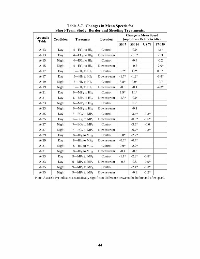
44

Table 3-7. Changes in Mean Speeds for Short-Term Study: Border and Sheeting Treatments.

Change in Mean Speed (mph) from Before to After Appendix

Table Condition Treatment Location SH 7 SH 14 US 79 FM 39

A-13 Day 4—EGS to HIR Control 0.0 1.1* A-13 Day 4—EGS to HIR Downstream -1.3* -0.3 A-15 Night 4—EGS to HIR Control -0.4 -0.2 A-15 Night 4—EGS to HIR Downstream -0.5 -2.0* A-17 Day 5—HIS to HIR Control 3.7* 1.2* 0.3* A-17 Day 5—HIS to HIR Downstream -1.7* -1.2* -3.8* A-19 Night 5—HIS to HIR Control 3.8* 0.9* -0.7 A-19 Night 5—HIS to HIR Downstream -0.6 -0.1 -4.3* A-21 Day 6—MPS to HIR Control 1.9* 1.1* A-21 Day 6—MPS to HIR Downstream -1.3* 0.0 A-23 Night 6—MPS to HIR Control 0.7 A-23 Night 6—MPS to HIR Downstream -0.1 A-25 Day 7—EGS to MPR Control -3.4* -1.3* A-25 Day 7—EGS to MPR Downstream -0.8* -1.6* A-27 Night 7—EGS to MPR Control -3.5* -0.6 A-27 Night 7—EGS to MPR Downstream -0.7* -1.3* A-29 Day 8—HIS to MPR Control 0.8* -2.2* A-29 Day 8—HIS to MPR Downstream -0.7* -0.7* A-31 Night 8—HIS to MPR Control 0.9* -2.2* A-31 Night 8—HIS to MPR Downstream -0.4 -0.3 A-33 Day 9—MPS to MPR Control -1.1* -2.3* -0.8* A-33 Day 9—MPS to MPR Downstream -0.3 0.5 -0.9* A-35 Night 9—MPS to MPR Control -2.4* -1.3* A-35 Night 9—MPS to MPR Downstream -0.3 -1.2*

Note: Asterisk (*) indicates a statistically significant difference between the before and after speed.

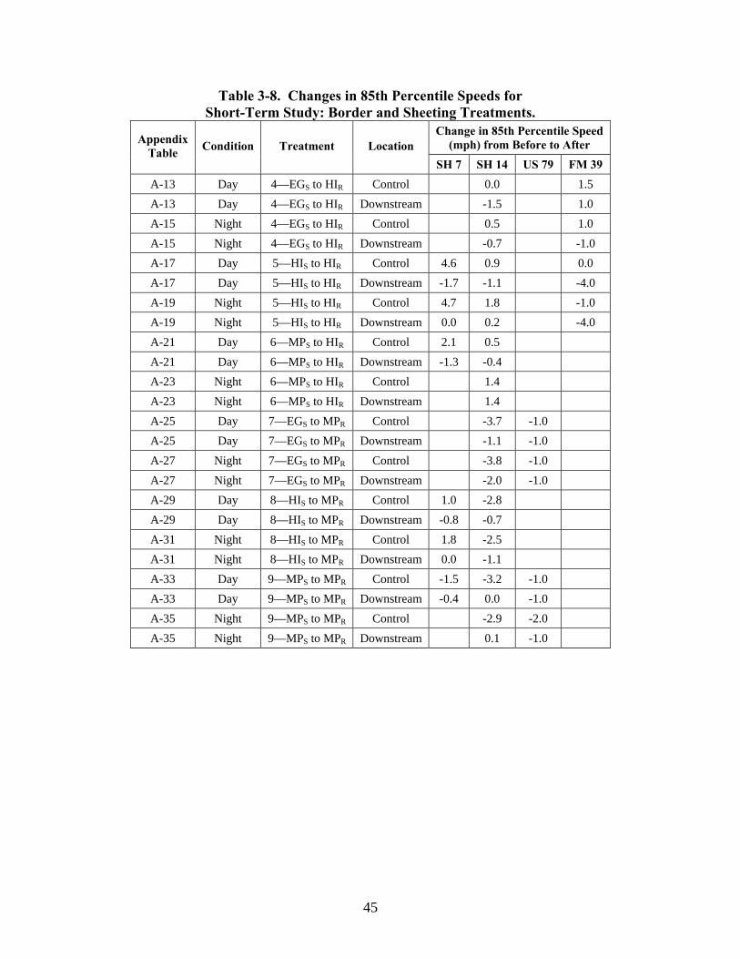
45

Table 3-8. Changes in 85th Percentile Speeds for Short-Term Study: Border and Sheeting Treatments.

Change in 85th Percentile Speed (mph) from Before to After Appendix

Table Condition Treatment Location SH 7 SH 14 US 79 FM 39

A-13 Day 4—EGS to HIR Control 0.0 1.5 A-13 Day 4—EGS to HIR Downstream -1.5 1.0 A-15 Night 4—EGS to HIR Control 0.5 1.0 A-15 Night 4—EGS to HIR Downstream -0.7 -1.0 A-17 Day 5—HIS to HIR Control 4.6 0.9 0.0 A-17 Day 5—HIS to HIR Downstream -1.7 -1.1 -4.0 A-19 Night 5—HIS to HIR Control 4.7 1.8 -1.0 A-19 Night 5—HIS to HIR Downstream 0.0 0.2 -4.0 A-21 Day 6—MPS to HIR Control 2.1 0.5 A-21 Day 6—MPS to HIR Downstream -1.3 -0.4 A-23 Night 6—MPS to HIR Control 1.4 A-23 Night 6—MPS to HIR Downstream 1.4 A-25 Day 7—EGS to MPR Control -3.7 -1.0 A-25 Day 7—EGS to MPR Downstream -1.1 -1.0 A-27 Night 7—EGS to MPR Control -3.8 -1.0 A-27 Night 7—EGS to MPR Downstream -2.0 -1.0 A-29 Day 8—HIS to MPR Control 1.0 -2.8 A-29 Day 8—HIS to MPR Downstream -0.8 -0.7 A-31 Night 8—HIS to MPR Control 1.8 -2.5 A-31 Night 8—HIS to MPR Downstream 0.0 -1.1 A-33 Day 9—MPS to MPR Control -1.5 -3.2 -1.0 A-33 Day 9—MPS to MPR Downstream -0.4 0.0 -1.0 A-35 Night 9—MPS to MPR Control -2.9 -2.0 A-35 Night 9—MPS to MPR Downstream 0.1 -1.0

46

Table 3-9. Changes in Percentage Exceeding 70/65 mph for Short-Term Study: Border and Sheeting Treatments.

Change in Percent Exceeding Appendix Table Condition Treatment Measure

SH 7 SH 14 US 79 FM 39 A-14 Day 4—EGS to HIR Control - -0.6 - 11.2 A-14 Day 4—EGS to HIR Downstream - 0.0 - 1.4 A-16 Night 4—EGS to HIR Control - -5.1 - -1.2 A-16 Night 4—EGS to HIR Downstream - 0.7 - -7.7 A-18 Day 5—HIS to HIR Control 27.9 7.9 - 0.9 A-18 Day 5—HIS to HIR Downstream -3.0 -0.6 - -10.4 A-20 Night 5—HIS to HIR Control 25.2 5.7 - -5.4 A-20 Night 5—HIS to HIR Downstream -0.1 1.4 - -14.9 A-22 Day 6—MPS to HIR Control 13.8 6.5 - - A-22 Day 6—MPS to HIR Downstream -3.0 0.3 - - A-24 Night 6—MPS to HIR Control - 5.4 - - A-24 Night 6—MPS to HIR Downstream - 2.9 - - A-26 Day 7—EGS to MPR Control - -23.4 -8.9 - A-26 Day 7—EGS to MPR Downstream - 0.3 -3.7 - A-28 Night 7—EGS to MPR Control - -30.4 -5.2 - A-28 Night 7—EGS to MPR Downstream - -3.7 -4.9 - A-30 Day 8—HIS to MPR Control 8.0 -14.8 - - A-30 Day 8—HIS to MPR Downstream -1.9 -0.3 - - A-32 Night 8—HIS to MPR Control 9.0 -19.7 - - A-32 Night 8—HIS to MPR Downstream 0.1 -3.0 - - A-34 Day 9—MPS to MPR Control -24.5 -16.3 -15.0 - A-34 Day 9—MPS to MPR Downstream -4.9 0.6 -2.0 - A-36 Night 9—MPS to MPR Control - -20.0 -8.0 - A-36 Night 9—MPS to MPR Downstream - -1.5 -8.4 -

Note: The speed limit was 70 mph for daytime and 65 mph for nighttime at the control point. The speed limit was 55 mph at the downstream point.

The final analysis of the short-term data was an assessment of the change in mean speeds

from the control point to the downstream point. Instead of comparing the change in speed

between two treatments at a given location, the researchers calculated the mean speed at the

control point and downstream point for a given treatment. The difference in these means was

used to define the effect of that treatment. Table 3-10 presents the results of this analysis. The

data analysis indicates that the largest decrease in speeds was realized with the red border

treatment with high intensity sheeting. However, the red border with microprismatic sheeting

47

did not show a benefit in comparison to the standard sign treatments. This analysis demonstrated

some value to the red border treatment, but not a consistent one.

Table 3-10. Change in Mean Speeds from Control to Downstream

Points for Short-Term Analysis. Daytime Nighttime

Site EGS HIS MPS HIR MPR EGS HIS MPS HIR MPR

SH 7 - 5.4 7.7 10.8 6.9 - 6.1 - 10.6 7.4

SH 14 9.6 8.4 9.7 10.8 6.9 9.4 8.5 8.8 9.5 6.7

US 79 8.0 - 8.2 - 8.3 6.2 - 7.0 - 6.9

FM 39 8.7 6.0 - 10.1 - 8.1 6.3 - 9.9 -

Average 8.8 6.6 8.5 10.6 7.4 7.9 7.0 7.9 10.0 7.0

RESULTS FOR LONG-TERM STUDY

The long-term study evaluated the change in speed at three sites (SH 21, SH 36, and

FM 60) that were previously evaluated in the first year of the project. During the first year, a red

border was added to standard Speed Limit signs at four sites. The red border treatment remained

in place at three of the sites following the initial collection of after data (short-term after) during

the first year. That allowed researchers to collect a second round of after data (long-term after)

approximately nine to twelve months after the treatments were installed. At these sites, the red

border was added by placing a solid blank covered with red microprismatic sheeting behind the

existing standard Speed Limit sign. The red sign blank was 6 inches wider and 6 inches taller

than the existing sign. There was no change in the standard Speed Limit sign between the

before, short-term after, and long-term after evaluations. The results for the before, short-term

after, and long-term after data collection at each site are given in Appendix B. These tables

present data by individual sites, comparing the measured speeds for before, short-term after, and

long-term after.

Table 3-11 compares the impacts of the short-term analysis with that of the long-term

analysis for the mean speeds. The speeds in this table represent the change in mean speed from

the before condition to either the short-term after or long-term after condition. The results

indicate that in every case but one, there is a larger reduction in the downstream mean speeds for

the long-term after condition than for the short-term after condition. In the one case where there

was a small increase in the downstream speed, there was a larger increase in the speed at the

48

control point. These results indicate that the red border treatment had a greater benefit on traffic

speeds a year or so after installation than it did immediately after installation.

Table 3-11. Change in Mean Speeds for Long-Term Study.

Location Condition Measure Short-Term Before Long-Term Before SH 21 Daytime Control 1.2* 1.0* SH 21 Daytime Downstream -1.0* -3.3* SH 21 Nighttime Control 0.7 2.0* SH 21 Nighttime Downstream -1.8* -1.6* SH 36 Daytime Control 2.1* 1.0* SH 36 Daytime Downstream -0.1 -5.6* SH 36 Nighttime Control 1.7 0.4 SH 36 Nighttime Downstream -0.1 -3.8* FM 60 Daytime Control 0.8 -3.0* FM 60 Daytime Downstream -0.1 -7.5* FM 60 Nighttime Control 1.4* -1.1* FM 60 Nighttime Downstream -0.6 -4.6*

The researchers also compared the changes in the 85th percentile speeds for the short-

term and long-term conditions. Table 3-12 indicates that the 85th percentile speeds at the

downstream location were higher for the long-term analysis than they were for the short-term

analysis. At two of the three sites, the speed reduction between the before and long-term after

conditions were several miles per hour greater than for the short-term condition. These results

also indicate a benefit to the red border treatment.

The third type of analysis of the long-term impacts of the first year study sites compared

the change in mean speeds between the control and downstream points for each of the three

study conditions: before, short-term after, and long-term after. Table 3-13 presents the results of

that analysis. The table shows that, for both the daytime and nighttime conditions, the speed

reduction shortly after installation (short-term analysis) was greater than the speed reduction

before installation and that the speed reduction approximately a year later was greater than it was

shortly after installation. These results clearly indicate the benefit of the red border treatment.

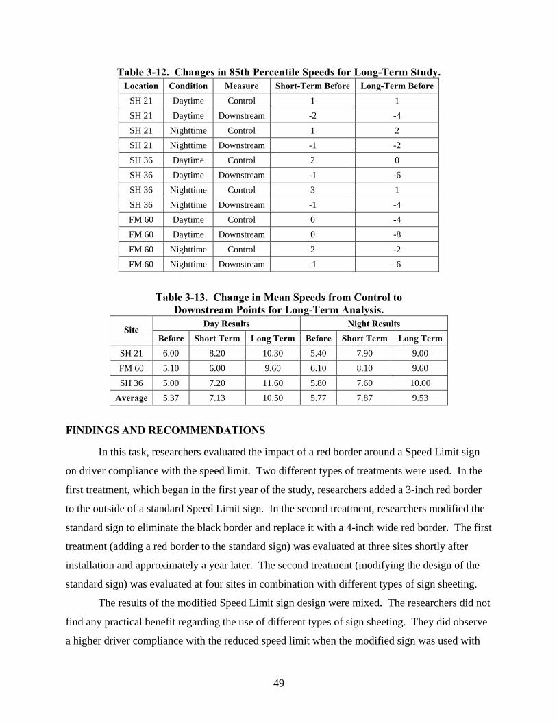
49

Table 3-12. Changes in 85th Percentile Speeds for Long-Term Study. Location Condition Measure Short-Term Before Long-Term Before

SH 21 Daytime Control 1 1 SH 21 Daytime Downstream -2 -4 SH 21 Nighttime Control 1 2 SH 21 Nighttime Downstream -1 -2 SH 36 Daytime Control 2 0 SH 36 Daytime Downstream -1 -6 SH 36 Nighttime Control 3 1 SH 36 Nighttime Downstream -1 -4 FM 60 Daytime Control 0 -4 FM 60 Daytime Downstream 0 -8 FM 60 Nighttime Control 2 -2 FM 60 Nighttime Downstream -1 -6

Table 3-13. Change in Mean Speeds from Control to Downstream Points for Long-Term Analysis.

Day Results Night Results Site

Before Short Term Long Term Before Short Term Long Term SH 21 6.00 8.20 10.30 5.40 7.90 9.00 FM 60 5.10 6.00 9.60 6.10 8.10 9.60 SH 36 5.00 7.20 11.60 5.80 7.60 10.00

Average 5.37 7.13 10.50 5.77 7.87 9.53

FINDINGS AND RECOMMENDATIONS

In this task, researchers evaluated the impact of a red border around a Speed Limit sign

on driver compliance with the speed limit. Two different types of treatments were used. In the

first treatment, which began in the first year of the study, researchers added a 3-inch red border

to the outside of a standard Speed Limit sign. In the second treatment, researchers modified the

standard sign to eliminate the black border and replace it with a 4-inch wide red border. The first

treatment (adding a red border to the standard sign) was evaluated at three sites shortly after

installation and approximately a year later. The second treatment (modifying the design of the

standard sign) was evaluated at four sites in combination with different types of sign sheeting.

The results of the modified Speed Limit sign design were mixed. The researchers did not

find any practical benefit regarding the use of different types of sign sheeting. They did observe

a higher driver compliance with the reduced speed limit when the modified sign was used with

50

high intensity sheeting. However, they did not find a similar benefit to using the red border with

microprismatic sheeting.

The results of the standard Speed Limit sign with the added red border were much

clearer. Both the short-term and the long-term analysis showed a greater driver compliance with

the downstream speed limit. The speed reduction between the control point and the downstream

point was much greater a year after installation than it had been shortly after installation.

Based on these findings, the researchers believe that it is appropriate to use the red border

treatment as a means of improving driver compliance with speed limits at locations where the

speed limit decreases on the approach to a city or town. The evaluation findings indicate that the

most effective means of implementing the red border is to simply add a 3-inch border to an

existing Speed Limit sign. According to information provided by the Federal Highway

Administration, such a conspicuity treatment does not require a change in the Texas MUTCD.

REFERENCES

1. Speeding. Traffic Safety Facts, National Highway Traffic Safety Administration,

Washington, D.C., 2003. http://www-nrd.nhtsa.dot.gov/pdf/nrd-

30/NCSA/TSF2003/809771.pdf. Accessed June 20, 2005.

2. Rose, E.R., H.G. Hawkins, and A.J. Holick. Evaluation of Traffic Control Devices: First

Year Activities. FHWA/TX-05/4701-1, Texas Transportation Institute, The Texas A&M

University System, College Station, Texas, 2004.

3. Noyce, D.A., X. Qin, and J.J. Guenette. The Effectiveness of Overhead Mounted

Regulatory Speed Signs on Operating Speed. www.topslab.wisc.edu/projects/

speed_sign_project_summary_report.pdf. Accessed June 20, 2005.

4. Traffic Advisory Leaflet: Vehicle Activated Signs. Department for Transport.

http://www.dft.gov.uk/stellent/groups/dft_roads/documents/page/dft_roads_508245.pdf.

Accessed June 2005.

5. Gates, T.J., H.G. Hawkins, S.T. Chrysler, P.J. Carlson, A.J. Holick, and C.H.

Spiegelman. Traffic Operational Impacts of Higher-Conspicuity Sign Materials. FHWA/

TX-04/4271-1, Texas Transportation Institute, The Texas A&M University System,

College Station, Texas, 2003.

http://www-nrd.nhtsa.dot.gov/pdf/nrd-30/NCSA/TSF2003/809771.pdf

http://www-nrd.nhtsa.dot.gov/pdf/nrd-30/NCSA/TSF2003/809771.pdf

http://www.dft.gov.uk/stellent/groups/dft_roads/documents/page/dft_roads_508245.pdf

www.topslab.wisc.edu/

51

CHAPTER 4: EFFECTIVENESS OF DEW-RESISTANT SHEETING

INTRODUCTION

Retroreflective sheeting is used on traffic signs so that the signs can convey information

to motorists at night. This sheeting uses either microsized glass beads or microsized prisms to

redirect light from a vehicle’s headlamps back toward the source, thereby illuminating the sign

for the driver to see. There are many factors that make it difficult for the light to get to the sign

or back to the vehicle, such as rain, snow, fog, or dirt. Dew and frost are also factors that impede

headlamp light from getting to the sign and redirected back toward the source. Dew and frost

scatter the headlamp light entering the sign and then scatter the light exiting the sign, thereby

significantly reducing the amount of light reaching the driver and making the sign less bright.

Dew forms in tiny droplets on the surface of the sign and scatters the light on its way to

the sign and then again as it leaves the sign. These droplets result in only a fraction of the light

making it to the driver’s eye and the sign appearing dark or even non-retroreflective. In order for

dew to form on the surface of the sign certain weather conditions need to be present. The skies

must be relatively clear so that heat loss from the sign due to radiations will occur. The air must

be still so that the sign remains at a lower temperature than the air, and the humidity must be

high (1).

The Avery Dennison Corporation has developed a prototype coating for retroreflective

sheeting materials that appear to have the ability to resist the formation of dew in a manner that

allows the retroreflection to continue to work as designed. This ability to resist dew formation

could be a useful breakthrough as traditional retroreflective sheeting materials lose practically all

of their ability to retroreflect as dew forms and as long as dew exists on the sign surface. The

loss of retroreflectivity at night is of particular concern to many agencies, and the only proven

solution to date has been illuminated signs, which is cost prohibitive in most cases.

The prototype coating developed by Avery Dennison was found by the manufacturer to

be effective under simulated laboratory conditions. However, there are several issues that still

needed to be addressed. The first issue was to determine how the new experimental sheeting

performs under real-world conditions on actual sign substrate and mounted in a manner similar

to that of a typical installation along the roadside. In other words, does the prototype coating

52

resist dew in outdoor conditions the same as under the simulated laboratory conditions? Other

questions of interest were:

• How do the sign substrate and the sign support system impact the development of

dew and the coatings’ performance?

• Do the dew-resistant characteristics of the coating perform consistently as it ages?

• What is the workability of the new sheeting with respect to sign fabrication and

handling?

• Finally, how well does the dew-resistant coating perform in terms of its ability to

maintain nighttime legibility/recognition of highway signs under dew conditions?

An initial pilot study was sponsored by the Texas Department of Transportation with the

cooperation of the Avery Dennison Corporation to allow testing of the new dew-resistant sign

sheeting at the Texas Transportation Institute’s (TTI) Riverside Campus. This chapter describes

the evaluation and the results.

Objective

The objective of this effort was to test the experimental sheeting under real-world

conditions on real sign substrate and mounted in a manner similar to that of a typical installation

along the roadside. If the experimental sheeting performed as anticipated based on laboratory

tests conducted by Avery Dennison scientists, then additional study would be warranted.

However, the effort described in this chapter was designed as a proof of concept only.

EXPERIMENTAL DESIGN

The goal of this evaluation was to assess how the prototype sheeting would affect dew

formation in real-world conditions in comparison to standard sheeting. The concept of the

evaluation was to fabricate an actual sign using both standard and dew-resistant sheeting, and

then to monitor and compare the performance of the sign in high-dew conditions.

Procedure

The basic concept of this effort was to monitor a sign with both regular retroreflective

sheeting and dew-resistant retroreflective sheeting in a real-world setting where the actual

weather conditions determined the formation of dew on the sign. A camera was set up to

53

automatically record pictures of the test sign in 15-minute increments. Researchers could then

review and analyze the pictures to determine the effectiveness of the dew-resistant sheeting.

Equipment

TTI designed a sign layout for the study that could be used to assess the effectiveness of

the dew-resistant materials as well as allowing evaluation of other aspects of signing (such as

legibility). Avery Dennison provided a sign fabricated according to the TTI specifications, a

camera, and a light emitting diode (LED) light source for the evaluation. Figure 4-1 illustrates

the test sign used in the evaluation. Figure 4-2 shows a photo of the camera and LED source (in

an environmental housing) used to record the sign images during dew formation conditions.

These two elements were installed approximately 60 feet from each other as illustrated in

Figure 4-3.

Figure 4-4 shows the design of the sign, indicating portions of the sign fabricated from

standard sheeting and portions fabricated from the prototype dew-resistant sheeting. The

background of the sign is green, and the legend and border are white. Avery Dennison Series

T7500 retroreflective sheeting was used for the entire sign, mounted on extruded aluminum. The

sign is 6 feet wide and 5 feet high. The C2 and C6 labels represent control material (or material

that has not been treated with the dew-resistant coating). The labels DR2 and DR6 represent

samples that have been treated with the dew-resistant coating. The left and bottom borders are

made with the control sheeting. The top and right borders are made with the dew-resistant

sheeting. The top left series of letters (BER) are made from sheeting without the dew-resistant

coating. The other three combinations of letters (BER) are made with the dew-resistant sheeting.

The left half of the panel is made with green T7500 sheeting. The right half of the panel is made

with green T7500 sheeting with the dew-resistant coating. It should be noted that only the four

rectangles in the middle of the sign were used for the analysis described herein.

The retroreflectivity of the sign was recorded using a handheld retroreflectometer with a

fixed geometry of 0.2/-4.0 degrees. The results of the retroreflectivity readings verified that the

material was T7500, or ASTM Type VIII. The average values of the white rectangles for two

different dates are shown in Table 4-1. The small changes in retroreflectivity values are typical

and not a cause for alarm.

54

Figure 4-1. Test Sign.

Figure 4-2. Camera and Light Source.

Note: Circles indicate sign and camera.

Figure 4-3. Experimental Setup.

Table 4-1. Measured Retroreflectivity Values (cd/lx/m2). Date of Readings Panel C2 Panel DR2 Panel C6 Panel DR6

August 13, 2004 981 1013 902 950

October 1, 2004 955 970 849 954

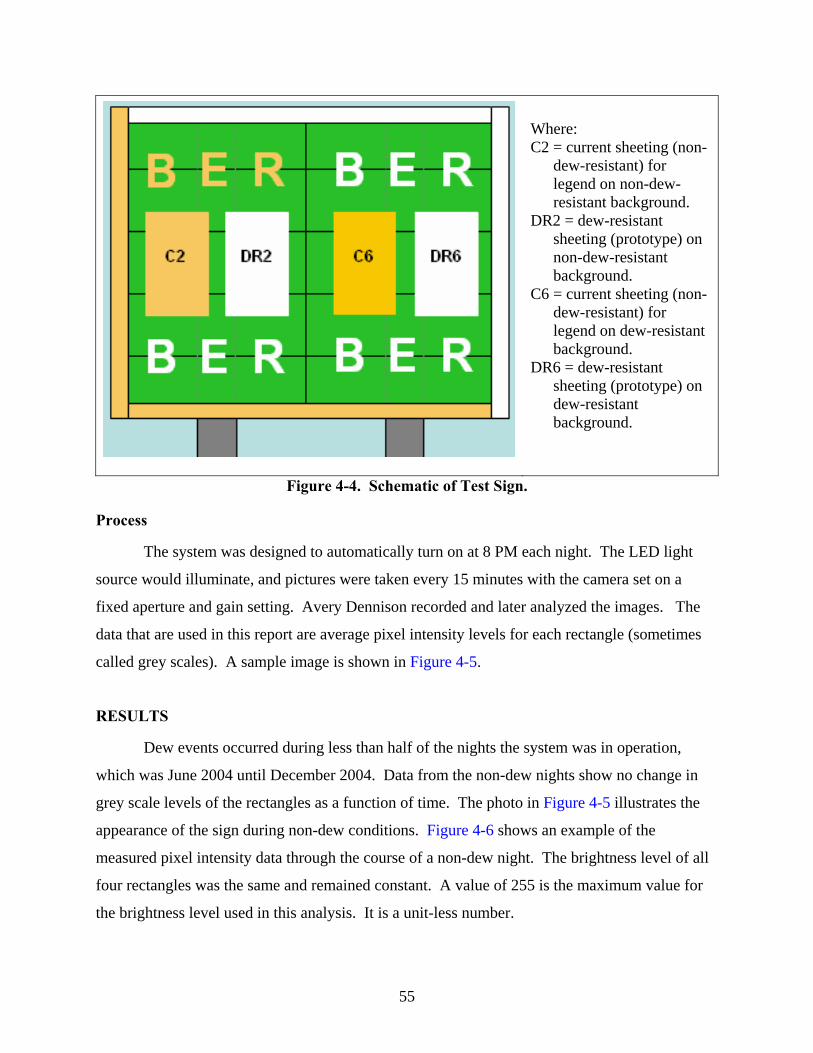
55

Where: C2 = current sheeting (non-

dew-resistant) for legend on non-dew-resistant background.

DR2 = dew-resistant sheeting (prototype) on non-dew-resistant background.

C6 = current sheeting (non-dew-resistant) for legend on dew-resistant background.

DR6 = dew-resistant sheeting (prototype) on dew-resistant background.

Figure 4-4. Schematic of Test Sign.

Process

The system was designed to automatically turn on at 8 PM each night. The LED light

source would illuminate, and pictures were taken every 15 minutes with the camera set on a

fixed aperture and gain setting. Avery Dennison recorded and later analyzed the images. The

data that are used in this report are average pixel intensity levels for each rectangle (sometimes

called grey scales). A sample image is shown in Figure 4-5.

RESULTS

Dew events occurred during less than half of the nights the system was in operation,

which was June 2004 until December 2004. Data from the non-dew nights show no change in

grey scale levels of the rectangles as a function of time. The photo in Figure 4-5 illustrates the

appearance of the sign during non-dew conditions. Figure 4-6 shows an example of the

measured pixel intensity data through the course of a non-dew night. The brightness level of all

four rectangles was the same and remained constant. A value of 255 is the maximum value for

the brightness level used in this analysis. It is a unit-less number.

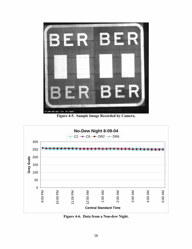
56

Figure 4-5. Sample Image Recorded by Camera.

No-Dew Night 8-09-04

0

50

100

150

200

250

300

9:00

PM

10:0

0 PM

11:0

0 PM

12:0

0 AM

1:00

AM

2:00

AM

3:00

AM

4:00

AM

5:00

AM

Central Standard Time

Gre

y Sc

ale

C2 C6 DR2 DR6

Figure 4-6. Data from a Non-dew Night.

57

Nights with recorded dew events were much more interesting. Figure 4-7 shows a series

of photos for a dew event representing the appearance of the sign at various times during the

night. As the evening wears on, it is apparent that the standard sheeting rectangles (non-dew-

resistant) are not as bright as the dew-resistant rectangles. Figure 4-8 presents a graphical

representation of dew formation on the same night. After 6 AM the sun began to rise and the

camera settings, which are set and fixed for dark conditions, are overexposed. Figure 4-9

presents a graphical representation of the data for a different dew night (June 30, 2004) and the

effectiveness of the dew-resistant sheeting materials.

10 PM 11 PM MIDNIGHT

1 AM 2 AM 3 AM

4 AM 5 AM 6 AM Figure 4-7. Hourly Representation of a Dew Event (July 11, 2004).

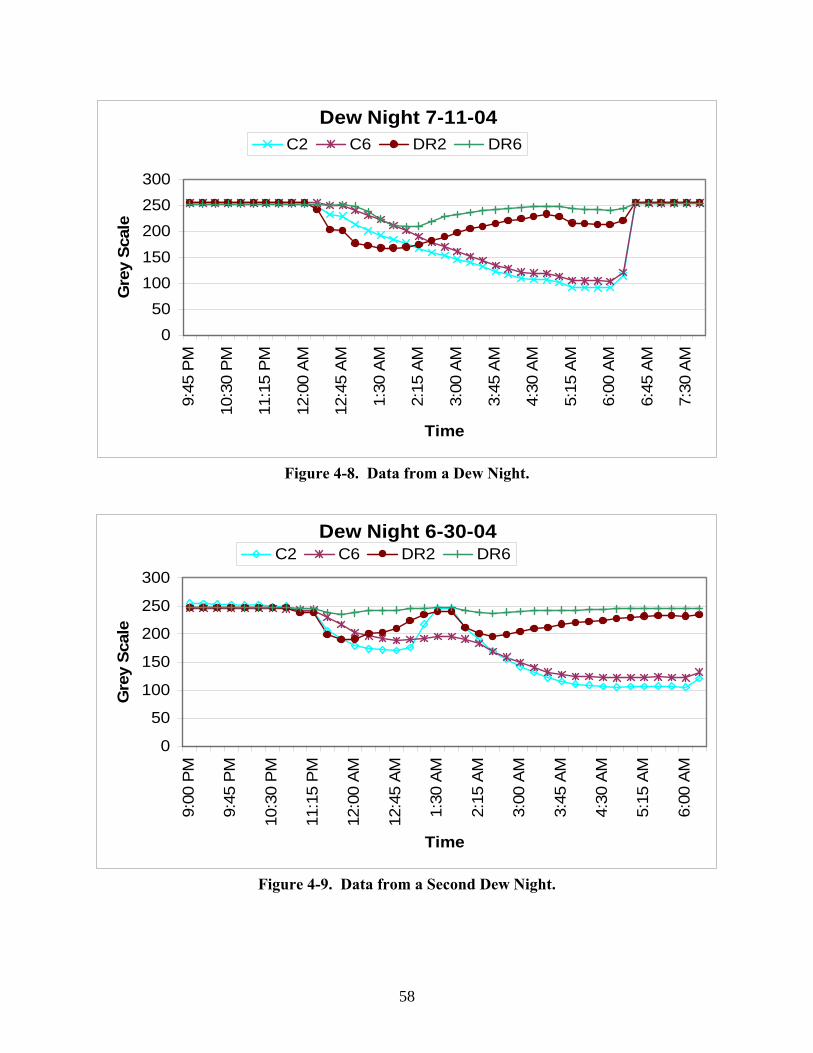
58

Figure 4-8. Data from a Dew Night.

Figure 4-9. Data from a Second Dew Night.

Dew Night 7-11-04

050

100150200250300

9:45

PM

10:3

0 P

M

11:1

5 P

M

12:0

0 A

M

12:4

5 A

M

1:30

AM

2:15

AM

3:00

AM

3:45

AM

4:30

AM

5:15

AM

6:00

AM

6:45

AM

7:30

AM

Time

Gre

y Sc

ale

C2 C6 DR2 DR6

Dew Night 6-30-04

0

50

100

150

200

250

300

9:00

PM

9:45

PM

10:3

0 P

M

11:1

5 P

M

12:0

0 A

M

12:4

5 A

M

1:30

AM

2:15

AM

3:00

AM

3:45

AM

4:30

AM

5:15

AM

6:00

AM

Time

Gre

y Sc

ale

C2 C6 DR2 DR6

59

While all dew events appear to be unique, the common theme is that the dew-resistant

sheeting appears to be effective in reducing the impacts of dew. Initially, the dew-resistant

material appears to degrade similar to the standard material. However, while the standard

material continues to degrade, the dew-resistant material begins to regain brightness and nearly

reaches full recovery. When the standard material has lost more than half of its effectiveness to

retroreflect, the dew-resistant material is working at close to 100 percent of its capability.

Figure 4-10 presents a good representation of the appearance of a sign under dew-forming

conditions.

Figure 4-10. Sign Appearance in Dew-Forming Conditions.

60

CONCLUSIONS AND RECOMMENDATIONS

The research described herein shows that the prototype dew-resistant sheeting tested in

this study is effective in reducing and nearly eliminating the negative impacts that dew has on

retroreflective traffic signs. The test sign was constructed in the same manner as any traffic sign

would be constructed. It was exposed to the elements as a normal traffic sign would be. And it

performed as expected based on the laboratory results provided by Avery Dennison, which

ultimately led to this research effort. It should be noted that the data presented herein are based

on a limited number of dew events. While it is expected that the performance of the material

would be similar in other dew events, the limited amount of available data limits prevents a

detailed analysis of the variability of the material’s performance over a range of conditions.

The next question that needs to be identified is the durability of the dew-resistant

properties. In others words, does the effectiveness diminish over time? If so, what is the life of

the dew-resistant properties? Would it impact handling of the signs or fabrication processes?

And finally, how would the material impact the recognition and legibility of traffic signs? These

questions should be explored with continued research efforts.

The data collected as part of this effort indicate that it appears possible to develop

products that have enhanced performance with respect to dew formation on the face of signs.

The material evaluated in this effort was a prototype material developed by Avery Dennison for

evaluation purposes. The evaluation found beneficial results, but several other factors still need

to be addressed. Avery Dennison continues to perform additional testing on the prototype

material, such as accelerated outdoor weathering in order to investigate durability. The next step

for this new technology would be to test its dew-resistant properties under different climatic

conditions in an actual road environment. If this material becomes available in the future, the

researchers recommend installing it at several field locations for a long-term trial. Nighttime

performance in high-dew conditions should be monitored, as well as the long-term durability of

the material.

REFERENCES

1. Hutchison, J.W., and T.A. Pullen. Performance of Signs under Dew and Frost Conditions, in Transportation Research Board 681, Transportation Research Board, Washington, D.C., 1978, pp. 16-20.

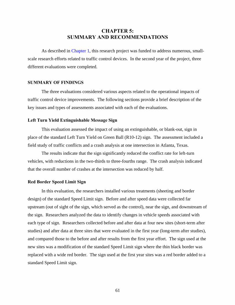
61

CHAPTER 5: SUMMARY AND RECOMMENDATIONS

As described in Chapter 1, this research project was funded to address numerous, small-

scale research efforts related to traffic control devices. In the second year of the project, three

different evaluations were completed.

SUMMARY OF FINDINGS

The three evaluations considered various aspects related to the operational impacts of

traffic control device improvements. The following sections provide a brief description of the

key issues and types of assessments associated with each of the evaluations.

Left Turn Yield Extinguishable Message Sign

This evaluation assessed the impact of using an extinguishable, or blank-out, sign in

place of the standard Left Turn Yield on Green Ball (R10-12) sign. The assessment included a

field study of traffic conflicts and a crash analysis at one intersection in Atlanta, Texas.

The results indicate that the sign significantly reduced the conflict rate for left-turn

vehicles, with reductions in the two-thirds to three-fourths range. The crash analysis indicated

that the overall number of crashes at the intersection was reduced by half.

Red Border Speed Limit Sign

In this evaluation, the researchers installed various treatments (sheeting and border

design) of the standard Speed Limit sign. Before and after speed data were collected far

upstream (out of sight of the sign, which served as the control), near the sign, and downstream of

the sign. Researchers analyzed the data to identify changes in vehicle speeds associated with

each type of sign. Researchers collected before and after data at four new sites (short-term after

studies) and after data at three sites that were evaluated in the first year (long-term after studies),

and compared those to the before and after results from the first year effort. The sign used at the

new sites was a modification of the standard Speed Limit sign where the thin black border was

replaced with a wide red border. The sign used at the first year sites was a red border added to a

standard Speed Limit sign.

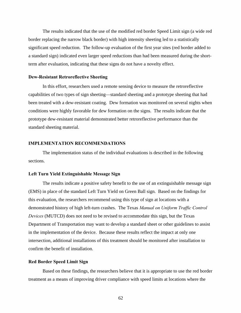
62

The results indicated that the use of the modified red border Speed Limit sign (a wide red

border replacing the narrow black border) with high intensity sheeting led to a statistically

significant speed reduction. The follow-up evaluation of the first year sites (red border added to

a standard sign) indicated even larger speed reductions than had been measured during the short-

term after evaluation, indicating that these signs do not have a novelty effect.

Dew-Resistant Retroreflective Sheeting

In this effort, researchers used a remote sensing device to measure the retroreflective

capabilities of two types of sign sheeting—standard sheeting and a prototype sheeting that had

been treated with a dew-resistant coating. Dew formation was monitored on several nights when

conditions were highly favorable for dew formation on the signs. The results indicate that the

prototype dew-resistant material demonstrated better retroreflective performance than the

standard sheeting material.

IMPLEMENTATION RECOMMENDATIONS

The implementation status of the individual evaluations is described in the following

sections.

Left Turn Yield Extinguishable Message Sign

The results indicate a positive safety benefit to the use of an extinguishable message sign

(EMS) in place of the standard Left Turn Yield on Green Ball sign. Based on the findings for

this evaluation, the researchers recommend using this type of sign at locations with a

demonstrated history of high left-turn crashes. The Texas Manual on Uniform Traffic Control

Devices (MUTCD) does not need to be revised to accommodate this sign, but the Texas

Department of Transportation may want to develop a standard sheet or other guidelines to assist

in the implementation of the device. Because these results reflect the impact at only one

intersection, additional installations of this treatment should be monitored after installation to

confirm the benefit of installation.

Red Border Speed Limit Sign

Based on these findings, the researchers believe that it is appropriate to use the red border

treatment as a means of improving driver compliance with speed limits at locations where the

63

speed limit decreases on the approach to a city or town. The evaluation findings indicate that the

most effective means of implementing the red border is to simply add a 3-inch border to an

existing Speed Limit sign. According to information provided by the Federal Highway

Administration, such a conspicuity treatment does not require a change in the Texas MUTCD.

Dew-Resistant Retroreflective Sheeting

The material evaluated in this effort is a prototype material that is not currently available

as a commercial product. If this material becomes available in the future, the researchers

recommend installing it at several field locations for a long-term trial. Nighttime performance in

high-dew conditions should be monitored, as well as the long-term durability of the material.

65

APPENDIX A: SHORT-TERM RED BORDER SPEED LIMIT SIGN RESULTS

The tables in this appendix present the results of the short-term analysis of the impacts of

the modified red border Speed Limit sign. The researchers collected data at four sites. The

study treatments represented various combinations of sign sheeting and a standard Speed Limit

sign or a modified red border Speed Limit sign.

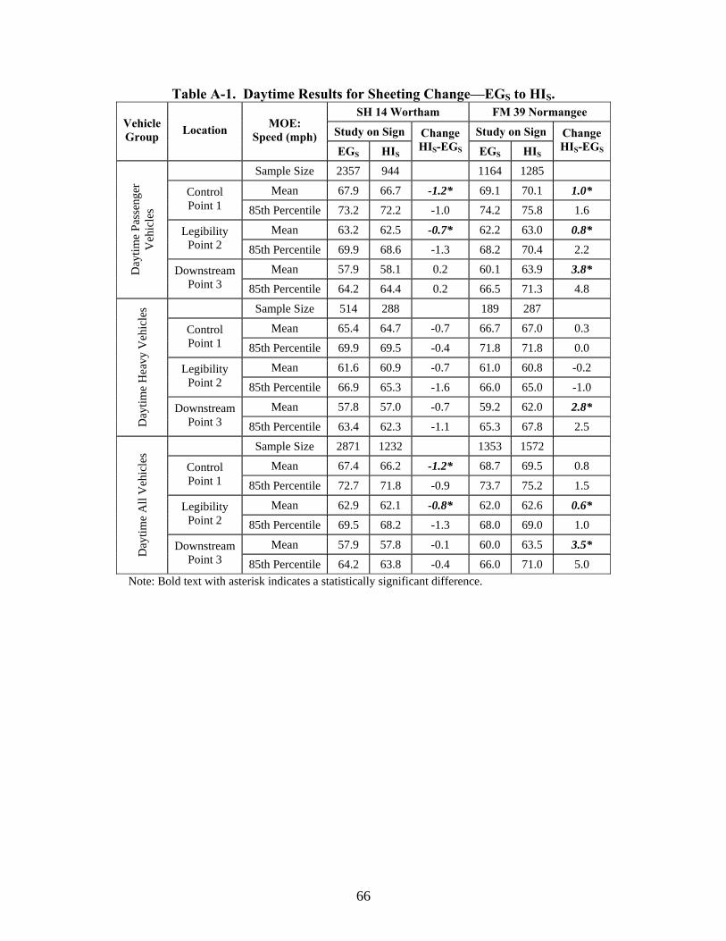
66

Table A-1. Daytime Results for Sheeting Change—EGS to HIS. SH 14 Wortham FM 39 Normangee

Study on Sign Study on Sign Vehicle Group Location MOE:

Speed (mph) EGS HIS

Change HIS-EGS EGS HIS

Change HIS-EGS

Sample Size 2357 944 1164 1285

Mean 67.9 66.7 -1.2* 69.1 70.1 1.0* Control Point 1 85th Percentile 73.2 72.2 -1.0 74.2 75.8 1.6

Mean 63.2 62.5 -0.7* 62.2 63.0 0.8* Legibility Point 2 85th Percentile 69.9 68.6 -1.3 68.2 70.4 2.2

Mean 57.9 58.1 0.2 60.1 63.9 3.8* Day

time

Pass

enge

r V

ehic

les

Downstream Point 3 85th Percentile 64.2 64.4 0.2 66.5 71.3 4.8

Sample Size 514 288 189 287

Mean 65.4 64.7 -0.7 66.7 67.0 0.3 Control Point 1 85th Percentile 69.9 69.5 -0.4 71.8 71.8 0.0

Mean 61.6 60.9 -0.7 61.0 60.8 -0.2 Legibility Point 2 85th Percentile 66.9 65.3 -1.6 66.0 65.0 -1.0

Mean 57.8 57.0 -0.7 59.2 62.0 2.8*

Day

time

Hea

vy V

ehic

les

Downstream Point 3 85th Percentile 63.4 62.3 -1.1 65.3 67.8 2.5

Sample Size 2871 1232 1353 1572

Mean 67.4 66.2 -1.2* 68.7 69.5 0.8 Control Point 1 85th Percentile 72.7 71.8 -0.9 73.7 75.2 1.5


Mean 57.9 57.8 -0.1 60.0 63.5 3.5*

Day

time

All

Veh

icle

s


Note: Bold text with asterisk indicates a statistically significant difference.

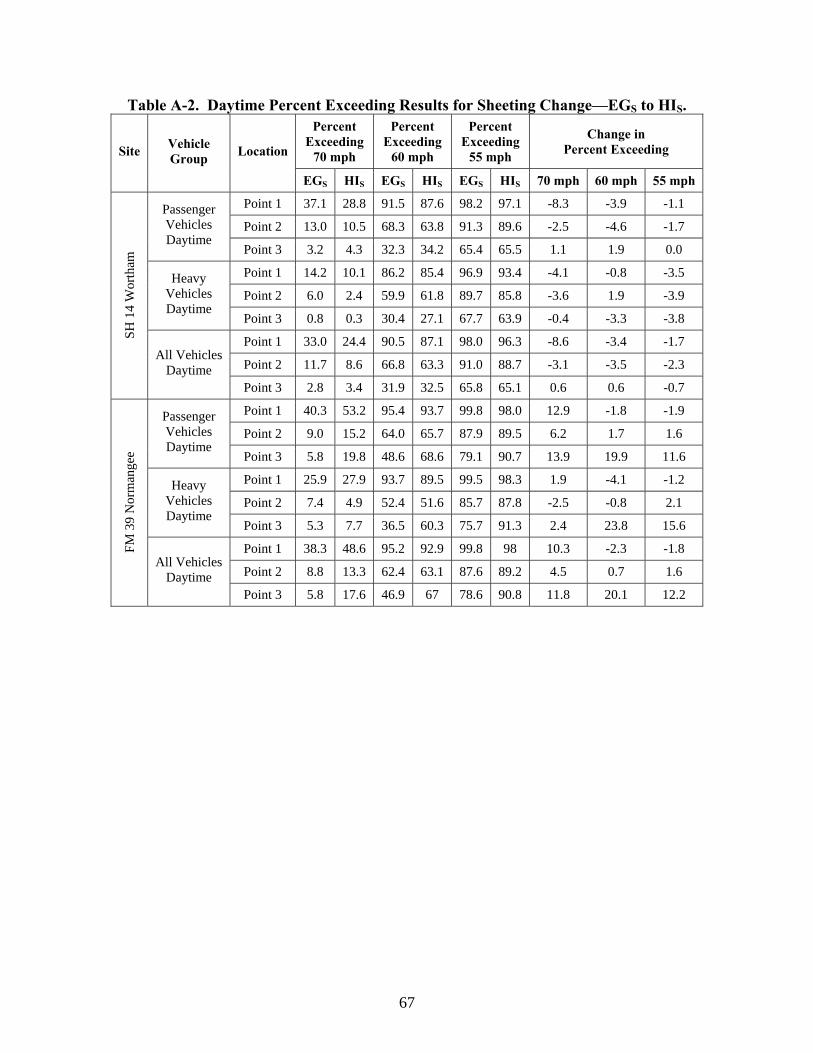
67

Table A-2. Daytime Percent Exceeding Results for Sheeting Change—EGS to HIS. Percent

Exceeding 70 mph

Percent Exceeding

60 mph

Percent Exceeding

55 mph

Change in Percent Exceeding Site Vehicle

Group Location

EGS HIS EGS HIS EGS HIS 70 mph 60 mph 55 mph

Point 1 37.1 28.8 91.5 87.6 98.2 97.1 -8.3 -3.9 -1.1

Point 2 13.0 10.5 68.3 63.8 91.3 89.6 -2.5 -4.6 -1.7 Passenger Vehicles Daytime

Point 3 3.2 4.3 32.3 34.2 65.4 65.5 1.1 1.9 0.0

Point 1 14.2 10.1 86.2 85.4 96.9 93.4 -4.1 -0.8 -3.5

Point 2 6.0 2.4 59.9 61.8 89.7 85.8 -3.6 1.9 -3.9 Heavy

Vehicles Daytime

Point 3 0.8 0.3 30.4 27.1 67.7 63.9 -0.4 -3.3 -3.8

Point 1 33.0 24.4 90.5 87.1 98.0 96.3 -8.6 -3.4 -1.7

Point 2 11.7 8.6 66.8 63.3 91.0 88.7 -3.1 -3.5 -2.3

SH 1

4 W

orth

am

All Vehicles Daytime

Point 3 2.8 3.4 31.9 32.5 65.8 65.1 0.6 0.6 -0.7

Point 1 40.3 53.2 95.4 93.7 99.8 98.0 12.9 -1.8 -1.9

Point 2 9.0 15.2 64.0 65.7 87.9 89.5 6.2 1.7 1.6 Passenger Vehicles Daytime

Point 3 5.8 19.8 48.6 68.6 79.1 90.7 13.9 19.9 11.6

Point 1 25.9 27.9 93.7 89.5 99.5 98.3 1.9 -4.1 -1.2

Point 2 7.4 4.9 52.4 51.6 85.7 87.8 -2.5 -0.8 2.1 Heavy

Vehicles Daytime

Point 3 5.3 7.7 36.5 60.3 75.7 91.3 2.4 23.8 15.6

Point 1 38.3 48.6 95.2 92.9 99.8 98 10.3 -2.3 -1.8

Point 2 8.8 13.3 62.4 63.1 87.6 89.2 4.5 0.7 1.6

FM 3

9 N

orm

ange

e


Point 3 5.8 17.6 46.9 67 78.6 90.8 11.8 20.1 12.2

68

Table A-3. Nighttime Results for Sheeting Change—EGS to HIS. SH 14 Wortham FM 39 Normangee


Speed (mph) EGS HIS

Change HIS-EGS EGS HIS

Change HIS-EGS

Sample Size 1562 402 309 236


Mean 60.4 59.0 -1.4* 61.6 61.4 -0.2 Legibility Point 2 85th Percentile 66.9 65.7 -1.2 66.8 67.3 0.5

Mean 55.6 55.1 -0.5 59.9 62.1 2.2* Nig

httim

e Pa

ssen

ger

Veh

icle

s


Sample Size 414 105 54 101

Mean 63.7 62.9 -0.8 65.4 66.8 1.4 Control Point 1 85th Percentile 68.6 67.3 -1.3 69.0 70.8 1.8

Mean 59.6 59.1 -0.5 60.8 60.9 0.1 Legibility Point 2 85th Percentile 64.9 64.0 -0.9 64.6 65.7 1.1

Mean 55.3 55.0 -0.3 59.7 62.1 2.4*

Nig

httim

e H

eavy

Veh

icle

s


Sample Size 1976 507 363 337


Mean 60.2 59.0 -1.2* 61.5 61.2 -0.3 Legibility Point 2 85th Percentile 66.4 65.3 -1.1 67.0 67.0 0.0

Mean 55.5 55.1 -0.4 59.8 62.1 2.3*

Nig

httim

e A

ll V

ehic

les



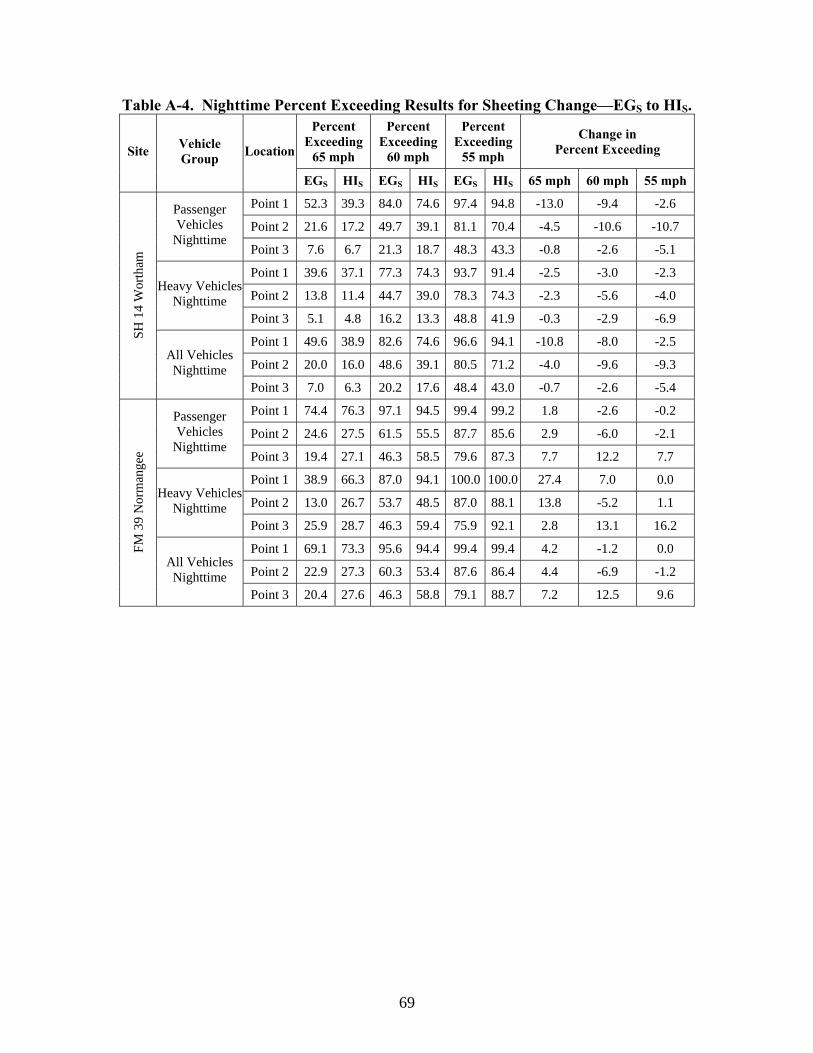
69

Table A-4. Nighttime Percent Exceeding Results for Sheeting Change—EGS to HIS. Percent

Exceeding 65 mph

Percent Exceeding

60 mph

Percent Exceeding

55 mph


Group Location

EGS HIS EGS HIS EGS HIS 65 mph 60 mph 55 mph

Point 1 52.3 39.3 84.0 74.6 97.4 94.8 -13.0 -9.4 -2.6

Point 2 21.6 17.2 49.7 39.1 81.1 70.4 -4.5 -10.6 -10.7 Passenger Vehicles

Nighttime Point 3 7.6 6.7 21.3 18.7 48.3 43.3 -0.8 -2.6 -5.1

Point 1 39.6 37.1 77.3 74.3 93.7 91.4 -2.5 -3.0 -2.3

Point 2 13.8 11.4 44.7 39.0 78.3 74.3 -2.3 -5.6 -4.0 Heavy Vehicles

Nighttime Point 3 5.1 4.8 16.2 13.3 48.8 41.9 -0.3 -2.9 -6.9

Point 1 49.6 38.9 82.6 74.6 96.6 94.1 -10.8 -8.0 -2.5

Point 2 20.0 16.0 48.6 39.1 80.5 71.2 -4.0 -9.6 -9.3

SH 1

4 W

orth

am

All Vehicles Nighttime

Point 3 7.0 6.3 20.2 17.6 48.4 43.0 -0.7 -2.6 -5.4

Point 1 74.4 76.3 97.1 94.5 99.4 99.2 1.8 -2.6 -0.2

Point 2 24.6 27.5 61.5 55.5 87.7 85.6 2.9 -6.0 -2.1 Passenger Vehicles

Nighttime Point 3 19.4 27.1 46.3 58.5 79.6 87.3 7.7 12.2 7.7

Point 1 38.9 66.3 87.0 94.1 100.0 100.0 27.4 7.0 0.0

Point 2 13.0 26.7 53.7 48.5 87.0 88.1 13.8 -5.2 1.1 Heavy Vehicles

Nighttime Point 3 25.9 28.7 46.3 59.4 75.9 92.1 2.8 13.1 16.2

Point 1 69.1 73.3 95.6 94.4 99.4 99.4 4.2 -1.2 0.0

Point 2 22.9 27.3 60.3 53.4 87.6 86.4 4.4 -6.9 -1.2

FM 3

9 N

orm

ange

e


Point 3 20.4 27.6 46.3 58.8 79.1 88.7 7.2 12.5 9.6

70

Table A-5. Daytime Results for Sheeting Change—EGS to MPS. SH 14 Wortham US 79 Oakwood


Speed (mph) EGS MPS

Change MPS-EGS EGS MPS

Change MPS-EGS

Sample Size 2357 1073 708 955

Mean 67.9 66.6 -1.3* 70.4 69.7 -0.7* Control Point 1 85th Percentile 73.2 72.2 -1.0 75 74 -1

Mean 63.2 60.4 -2.8* 68.8 66 -2.8* Legibility Point 2 85th Percentile 69.9 67.3 -2.6 75 72 -3

Mean 57.9 56.7 -1.2* 62 61.4 -0.6 Day

time

Pass

enge

r V

ehic

les

Downstream Point 3 85th Percentile 64.2 63.4 -0.8 69 68 -1

Sample Size 514 216 156 347

Mean 65.4 64.9 -0.5 67.2 68.1 0.9 Control Point 1 85th Percentile 69.9 70.4 0.5 71 72 1

Mean 61.6 59.5 -2.1* 66.7 64.1 -2.6* Legibility Point 2 85th Percentile 66.9 64.9 -2.0 71 69 -2

Mean 57.8 56.4 -1.4* 61.1 60.1 -1

Day

time

Hea

vy V

ehic

les


Sample Size 2871 1289 864 1302

Mean 67.4 66.3 -1.1* 69.8 69.3 -0.5* Control Point 1 85th Percentile 72.7 72.2 -0.5 74 74 0

Mean 62.9 60.2 -2.7* 68.5 65.5 -3* Legibility Point 2 85th Percentile 69.5 66.9 -2.6 74 71 -3

Mean 57.9 56.6 -1.3* 61.8 61.1 -0.7*

Day

time

All

Veh

icle

s

Downstream Point 3 85th Percentile 64.2 63.1 -1.10 68 68 0


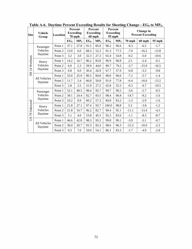
71

Table A-6. Daytime Percent Exceeding Results for Sheeting Change—EGS to MPS. Percent

Exceeding70 mph

Percent Exceeding

60 mph

Percent Exceeding

55 mph


Group Location

EGS MPS EGS MPS EGS MPS 70 mph 60 mph 55 mph Point 1 37.1 27.8 91.5 85.0 98.2 96.6 -9.3 -6.5 -1.7 Point 2 13.0 6.0 68.3 52.2 91.3 77.5 -7.0 -16.2 -13.8

Passenger Vehicles Daytime Point 3 3.2 3.0 32.3 27.3 65.4 54.8 -0.2 -5.0 -10.6

Point 1 14.2 16.7 86.2 83.8 96.9 96.8 2.5 -2.4 -0.1 Point 2 6.0 2.3 59.9 44.0 89.7 79.2 -3.7 -15.9 -10.5

Heavy Vehicles Daytime Point 3 0.8 0.0 30.4 26.9 67.7 57.9 -0.8 -3.5 -9.8

Point 1 33.0 25.9 90.5 84.8 98.0 96.6 -7.1 -5.7 -1.4 Point 2 11.7 5.4 66.8 50.8 91.0 77.8 -6.4 -16.0 -13.2

SH 1

4 W

orth

am


Point 3 2.8 2.5 31.9 27.2 65.8 55.3 -0.3 -4.7 -10.5 Point 1 52.1 48.5 98.4 95.7 99.7 99.2 -3.6 -2.7 -0.5 Point 2 39.1 24.4 92.7 83.5 98.4 96.8 -14.7 -9.2 -1.6

Passenger Vehicles Daytime Point 3 10.2 8.9 60.2 57.3 84.8 83.2 -1.3 -2.9 -1.6

Point 1 21.8 27.1 97.4 93.7 100.0 98.8 5.3 -3.8 -1.2 Point 2 21.8 10.7 96.2 82.7 99.4 95.1 -11.1 -13.4 -4.3

Heavy Vehicles Daytime Point 3 5.1 4.0 53.8 45.5 92.3 83.6 -1.1 -8.3 -8.7

Point 1 46.6 42.8 98.3 95.2 99.8 99.1 -3.9 -3.1 -0.7 Point 2 36.0 20.7 93.3 83.3 98.6 96.3 -15.3 -10.0 -2.3

US

79 O

akw

ood


Point 3 9.3 7.6 59.0 54.1 86.1 83.3 -1.7 -4.9 -2.8

72

Table A-7. Nighttime Results for Sheeting Change—EGS to MPS. SH 14 Wortham US 79 Oakwood


Speed (mph) EGS MPS

Change MPS-EGS EGS MPS

Change MPS-EGS

Sample Size 1562 212 387 267

Mean 65.2 63.7 -1.5* 68 68.7 0.7 Control Point 1 85th Percentile 69.9 69.0 -0.9 72 74 2

Mean 60.4 57.9 -2.5* 67.6 66 -1.6* Legibility Point 2 85th Percentile 66.9 64.2 -2.7 74 72 -2

Mean 55.6 54.6 -1.0* 61.9 61.3 -0.6 Nig

httim

e Pa

ssen

ger

Veh

icle

s


Sample Size 414 79 103 134

Mean 63.7 64.0 0.4 65.6 67.2 1.6* Control Point 1 85th Percentile 68.6 69.2 0.6 68 71 3

Mean 59.6 58.5 -1.1 65.2 65.3 0.1 Legibility Point 2 85th Percentile 64.9 62.8 -2.1 69 70 1

Mean 55.3 56.4 1.1 59.2 60.9 1.7

Nig

httim

e H

eavy

Veh

icle

s

Downstream Point 3 85th Percentile 60.9 62.0 1.1 65 67 2

Sample Size 1976 291 490 401

Mean 64.9 63.8 -1.1* 67.5 68.2 0.7 Control Point 1 85th Percentile 69.9 69.0 -0.9 72 73 1

Mean 60.2 58.0 -2.2* 67.1 65.8 -1.3* Legibility Point 2 85th Percentile 66.4 63.8 -2.6 73 71 -2

Mean 55.5 55.1 -0.4 61.3 61.2 -0.1

Nig

httim

e A

ll V

ehic

les

Downstream Point 3 85th Percentile 61.9 59.8 -2.2 68 68 0


73

Table A-8. Nighttime Percent Exceeding Results for Sheeting Change—EGS to MPS. Percent

Exceeding65 mph

Percent Exceeding

60 mph

Percent Exceeding

55 mph


Group Location

EGS MPS EGS MPS EGS MPS 65 mph 60 mph 55 mph Point 1 52.3 41.5 84.0 73.6 97.4 93.4 -10.8 -10.4 -4.0 Point 2 21.6 9.9 49.7 32.1 81.1 60.4 -11.7 -17.6 -20.7

Passenger Vehicles

Nighttime Point 3 7.6 5.2 21.3 10.8 48.3 40.6 -2.4 -10.4 -7.8 Point 1 39.6 32.9 77.3 78.5 93.7 94.9 -6.7 1.2 1.2 Point 2 13.8 5.1 44.7 35.4 78.3 73.4 -8.7 -9.2 -4.8

Heavy Vehicles

Nighttime Point 3 5.1 3.8 16.2 22.8 48.8 58.2 -1.3 6.6 9.4 Point 1 49.6 39.2 82.6 74.9 96.6 93.8 -10.5 -7.7 -2.8 Point 2 20.0 8.6 48.6 33.0 80.5 63.9 -11.4 -15.6 -16.6

SH 1

4 W

orth

am


Point 3 7.0 4.8 20.2 14.1 48.4 45.4 -2.2 -6.1 -3.1 Point 1 72.4 75.9 97.4 95.9 99.7 99.2 3.5 -1.5 -0.5 Point 2 67.2 56.8 89.1 85.0 98.7 95.5 -10.4 -4.1 -3.2

Passenger Vehicles

Nighttime Point 3 28.2 30.5 60.5 53.8 85.0 82.0 2.3 -6.7 -3.0 Point 1 54.4 61.9 96.1 93.3 100.0 100.0 7.6 -2.8 0.0 Point 2 54.4 47.0 90.3 80.6 98.1 98.5 -7.4 -9.7 0.4

Heavy Vehicles

Nighttime Point 3 12.6 24.6 42.7 49.3 77.7 80.6 12.0 6.5 2.9 Point 1 68.6 71.3 97.1 95.0 99.8 99.5 2.8 -2.1 -0.3 Point 2 64.5 53.6 89.4 83.5 98.6 96.5 -10.9 -5.8 -2.1

US

79 O

akw

ood


Point 3 24.9 28.4 56.7 52.1 83.5 81.5 3.5 -4.6 -1.9

74

Table A-9. Daytime Results for Sheeting Change—HIS to MPS. SH 14 Wortham SH 7 Marlin


Speed (mph) HIS MPS

Change MPS-HIS HIS MPS

Change HIR-HIS

Sample Size 944 1073 4166 471

Mean 66.7 66.6 -0.1 67.2 69.3 2.1* Control Point 1 85th Percentile 72.2 72.2 0.0 72.2 75.2 3.0


Mean 58.1 56.7 -1.4* 61.7 61.2 -0.5 Day

time

Pass

enge

r V

ehic

les

Downstream Point 3 85th Percentile 64.4 63.4 -1.0 69.0 68.8 -0.2

Sample Size 288 216 487 83

Mean 64.7 64.9 0.2 66.1 67.4 1.3 Control Point 1 85th Percentile 69.5 70.4 0.9 71.3 71.8 0.5

Mean 60.9 59.5 -1.4 64.5 73.7 9.2* Legibility Point 2 85th Percentile 65.3 64.9 -0.4 70.0 79.9 9.9

Mean 57.0 56.4 -0.7 61.9 61.9 0.0

Day

time

Hea

vy V

ehic

les


Sample Size 1232 1289 4653 554

Mean 66.2 66.3 0.1 67.1 69.0 1.9* Control Point 1 85th Percentile 71.8 72.2 0.4 72.2 74.7 2.5


Mean 57.8 56.6 -1.2* 61.7 61.3 -0.4

Day

time

All

Veh

icle

s



75

Table A-10. Daytime Percent Exceeding Results for Sheeting Change—HIS to MPS. Percent

Exceeding70 mph

Percent Exceeding

60 mph

Percent Exceeding

55 mph


Group Location

HIS MPS HIS MPS HIS MPS 70 mph 60 mph 55 mph

Point 1 28.8 27.8 87.6 85.0 97.1 96.6 -1.0 -2.6 -0.6


Point 3 4.3 3.0 34.2 27.3 65.5 54.8 -1.4 -6.9 -10.7

Point 1 10.1 16.7 85.4 83.8 93.4 96.8 6.6 -1.6 3.4

Point 2 2.4 2.3 61.8 44.0 85.8 79.2 -0.1 -17.8 -6.6 Heavy

Vehicles Daytime

Point 3 0.3 0.0 27.1 26.9 63.9 57.9 -0.3 -0.2 -6.0

Point 1 24.4 25.9 87.1 84.8 96.3 96.6 1.5 -2.3 0.3

Point 2 8.6 5.4 63.3 50.8 88.7 77.8 -3.3 -12.5 -10.9

SH 1

4 W

orth

am


Point 3 3.4 2.5 32.5 27.2 65.1 55.3 -0.9 -5.3 -9.8

Point 1 30.8 47.1 88.3 91.7 97.0 97.7 16.3 3.4 0.7


Point 3 11.1 11.7 57.0 54.1 82.4 78.8 0.6 -2.9 -3.6

Point 1 23.4 27.7 86.9 90.4 96.1 98.8 4.3 3.5 2.7

Point 2 15.0 72.3 78.9 98.8 95.1 100.0 57.3 19.9 4.9 Heavy

Vehicles Daytime

Point 3 9.7 7.2 61.0 59.0 86.2 90.4 -2.4 -1.9 4.1

Point 1 30.1 44.2 88.2 91.5 96.9 97.8 14.2 3.3 1.0

Point 2 19.6 69.7 77.3 97.5 94.3 99.8 50.1 20.2 5.6

SH 7

Mar

lin


Point 3 10.9 11.0 57.4 54.9 82.8 80.5 0.1 -2.6 -2.3

76

Table A-11. Nighttime Results for Sheeting Change—HIS to MPS. SH 14 Wortham

Study on Sign Vehicle Group Location MOE:

Speed (mph) HIS MPS

Change MPS-HIS

Sample Size 402 212

Mean 63.8 63.7 0.0 Control Point 1 85th Percentile 69.0 69.0 0.0

Mean 59.0 57.9 -1.2* Legibility Point 2 85th Percentile 65.7 64.2 -1.5

Mean 55.1 54.6 -0.5 Nig

httim

e Pa

ssen

ger

Veh

icle

s

DownstreamPoint 3 85th Percentile 61.3 59.0 -2.3

Sample Size 105 79


Mean 59.1 58.5 -0.6 Legibility Point 2 85th Percentile 64.0 62.8 -1.1

Mean 55.0 56.4 1.4

Nig

httim

e H

eavy

Veh

icle

s

DownstreamPoint 3 85th Percentile 59.2 62.0 2.8

Sample Size 507 291


Mean 59.0 58.0 -1.0* Legibility Point 2 85th Percentile 65.3 63.8 -1.5

Mean 55.1 55.1 0.0

Nig

httim

e A

ll V

ehic

les



77

Table A-12. Nighttime Percent Exceeding Results for Sheeting Change—HIS to MPS. Percent

Exceeding65 mph

Percent Exceeding

60 mph

Percent Exceeding

55 mph


Group Location

HIS MPS HIS MPS HIS MPS 65 mph 60 mph 55 mph Point 1 39.3 41.5 74.6 73.6 94.8 93.4 2.2 -1.0 -1.4 Point 2 17.2 9.9 39.1 32.1 70.4 60.4 -7.3 -7.0 -10.0

Passenger Vehicles

Nighttime Point 3 6.7 5.2 18.7 10.8 43.3 40.6 -1.5 -7.8 -2.7 Point 1 37.1 32.9 74.3 78.5 91.4 94.9 -4.2 4.2 3.5 Point 2 11.4 5.1 39.0 35.4 74.3 73.4 -6.4 -3.6 -0.9

Heavy Vehicles

Nighttime Point 3 4.8 3.8 13.3 22.8 41.9 58.2 -1.0 9.5 16.3 Point 1 38.9 39.2 74.6 74.9 94.1 93.8 0.3 0.4 -0.3 Point 2 16.0 8.6 39.1 33.0 71.2 63.9 -7.4 -6.1 -7.3

SH 1

4 W

orth

am


Point 3 6.3 4.8 17.6 14.1 43.0 45.4 -1.5 -3.5 2.4

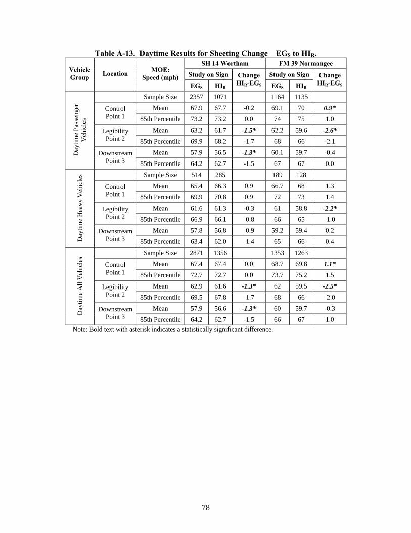
78

Table A-13. Daytime Results for Sheeting Change—EGS to HIR. SH 14 Wortham FM 39 Normangee


Speed (mph) EGS HIR

Change HIR-EGS EGS HIR

Change HIR-EGS

Sample Size 2357 1071 1164 1135

Mean 67.9 67.7 -0.2 69.1 70 0.9* Control Point 1 85th Percentile 73.2 73.2 0.0 74 75 1.0

Mean 63.2 61.7 -1.5* 62.2 59.6 -2.6* Legibility Point 2 85th Percentile 69.9 68.2 -1.7 68 66 -2.1

Mean 57.9 56.5 -1.3* 60.1 59.7 -0.4 Day

time

Pass

enge

r V

ehic

les

Downstream Point 3 85th Percentile 64.2 62.7 -1.5 67 67 0.0

Sample Size 514 285 189 128

Mean 65.4 66.3 0.9 66.7 68 1.3 Control Point 1 85th Percentile 69.9 70.8 0.9 72 73 1.4

Mean 61.6 61.3 -0.3 61 58.8 -2.2* Legibility Point 2 85th Percentile 66.9 66.1 -0.8 66 65 -1.0

Mean 57.8 56.8 -0.9 59.2 59.4 0.2

Day

time

Hea

vy V

ehic

les


Sample Size 2871 1356 1353 1263


Mean 62.9 61.6 -1.3* 62 59.5 -2.5* Legibility Point 2 85th Percentile 69.5 67.8 -1.7 68 66 -2.0

Mean 57.9 56.6 -1.3* 60 59.7 -0.3

Day

time

All

Veh

icle

s



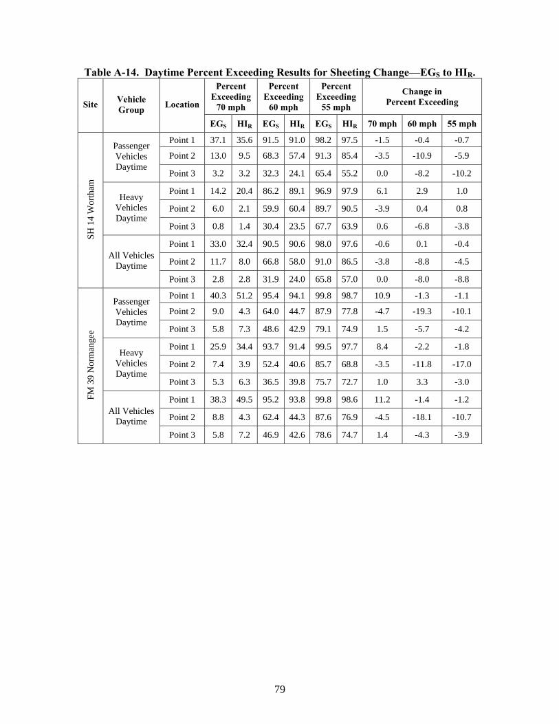
79

Table A-14. Daytime Percent Exceeding Results for Sheeting Change—EGS to HIR. Percent

Exceeding70 mph

Percent Exceeding

60 mph

Percent Exceeding

55 mph


Group Location

EGS HIR EGS HIR EGS HIR 70 mph 60 mph 55 mph

Point 1 37.1 35.6 91.5 91.0 98.2 97.5 -1.5 -0.4 -0.7


Point 3 3.2 3.2 32.3 24.1 65.4 55.2 0.0 -8.2 -10.2

Point 1 14.2 20.4 86.2 89.1 96.9 97.9 6.1 2.9 1.0

Point 2 6.0 2.1 59.9 60.4 89.7 90.5 -3.9 0.4 0.8 Heavy

Vehicles Daytime

Point 3 0.8 1.4 30.4 23.5 67.7 63.9 0.6 -6.8 -3.8

Point 1 33.0 32.4 90.5 90.6 98.0 97.6 -0.6 0.1 -0.4

Point 2 11.7 8.0 66.8 58.0 91.0 86.5 -3.8 -8.8 -4.5

SH 1

4 W

orth

am


Point 3 2.8 2.8 31.9 24.0 65.8 57.0 0.0 -8.0 -8.8

Point 1 40.3 51.2 95.4 94.1 99.8 98.7 10.9 -1.3 -1.1


Point 3 5.8 7.3 48.6 42.9 79.1 74.9 1.5 -5.7 -4.2

Point 1 25.9 34.4 93.7 91.4 99.5 97.7 8.4 -2.2 -1.8

Point 2 7.4 3.9 52.4 40.6 85.7 68.8 -3.5 -11.8 -17.0 Heavy

Vehicles Daytime

Point 3 5.3 6.3 36.5 39.8 75.7 72.7 1.0 3.3 -3.0

Point 1 38.3 49.5 95.2 93.8 99.8 98.6 11.2 -1.4 -1.2

Point 2 8.8 4.3 62.4 44.3 87.6 76.9 -4.5 -18.1 -10.7

FM 3

9 N

orm

ange

e


Point 3 5.8 7.2 46.9 42.6 78.6 74.7 1.4 -4.3 -3.9

80

Table A-15. Nighttime Results for Sheeting Change—EGS to HIR. SH 14 Wortham FM 39 Normangee


Speed (mph) EGS HIR

Change HIR-EGS EGS HIR

Change HIR-EGS

Sample Size 1562 275 309 221

Mean 65.2 64.6 -0.6 68.4 68 -0.4 Control Point 1 85th Percentile 69.9 70.4 0.5 73 74 1.0

Mean 60.4 59.3 -1.1* 61.6 57.9 -3.7* Legibility Point 2 85th Percentile 66.9 66.1 -0.8 67 65 -2.2

Mean 55.6 54.8 -0.8* 59.9 57.8 -2.1* Nig

httim

e Pa

ssen

ger

Veh

icle

s

Downstream Point 3 85th Percentile 62.0 60.6 -1.4 66 65 -1.2

Sample Size 414 75 54 47

Mean 63.7 64.3 0.7 65.4 66.2 0.8 Control Point 1 85th Percentile 68.6 68.5 -0.1 69 71 1.6

Mean 59.6 59.8 0.3 60.8 58.1 -2.7* Legibility Point 2 85th Percentile 64.9 66.4 1.5 65 62 -2.5

Mean 55.3 55.7 0.4 59.7 57.9 -1.8

Nig

httim

e H

eavy

Veh

icle

s

Downstream Point 3 85th Percentile 60.9 61.3 0.4 65 63 -2.5

Sample Size 1976 350 363 268

Mean 64.9 64.5 -0.4 67.9 67.7 -0.2 Control Point 1 85th Percentile 69.9 70.4 0.5 73 74 1.0

Mean 60.2 59.4 -0.8* 61.5 58 -3.5* Legibility Point 2 85th Percentile 66.4 66.1 -0.3 67 64 -3.0

Mean 55.5 55.0 -0.5 59.8 57.8 -2.0*

Nig

httim

e A

ll V

ehic

les

Downstream Point 3 85th Percentile 61.9 61.2 -0.7 66 65 -1.0


81

Table A-16. Nighttime Percent Exceeding Results for Sheeting Change—EGS to HIR. Percent

Exceeding65 mph

Percent Exceeding

60 mph

Percent Exceeding

55 mph


Group Location

EGS HIR EGS HIR EGS HIR 65 mph 60 mph 55 mph

Point 1 52.3 44.0 84.0 79.6 97.4 93.5 -8.3 -4.4 -3.9


Nighttime Point 3 7.6 7.6 21.3 18.5 48.3 41.1 0.1 -2.7 -7.2

Point 1 39.6 46.7 77.3 76.0 93.7 97.3 7.1 -1.3 3.6

Point 2 13.8 20.0 44.7 40.0 78.3 84.0 6.2 -4.7 5.7 Heavy

Vehicles Nighttime

Point 3 5.1 8.0 16.2 20.0 48.8 46.7 2.9 3.8 -2.1

Point 1 49.6 44.6 82.6 78.9 96.6 94.3 -5.1 -3.7 -2.3

Point 2 20.0 18.0 48.6 43.4 80.5 74.0 -2.0 -5.2 -6.5

SH 1

4 W

orth

am


Point 3 7.0 7.7 20.2 18.9 48.4 42.3 0.7 -1.3 -6.1

Point 1 74.4 71.0 97.1 89.6 99.4 97.3 -3.4 -7.5 -2.1


Nighttime Point 3 19.4 13.6 46.3 32.1 79.6 63.3 -5.8 -14.2 -16.3

Point 1 38.9 53.2 87.0 89.4 100.0 100.0 14.3 2.3 0.0

Point 2 13.0 6.4 53.7 31.9 87.0 72.3 -6.6 -21.8 -14.7 Heavy

Vehicles Nighttime

Point 3 25.9 8.5 46.3 29.8 75.9 76.6 -17.4 -16.5 0.7

Point 1 69.1 67.9 95.6 89.6 99.4 97.8 -1.2 -6.0 -1.6

Point 2 22.9 10.8 60.3 34.3 87.6 68.3 -12.1 -26.0 -19.3

FM 3

9 N

orm

ange

e


Point 3 20.4 12.7 46.3 31.7 79.1 65.7 -7.7 -14.6 -13.4

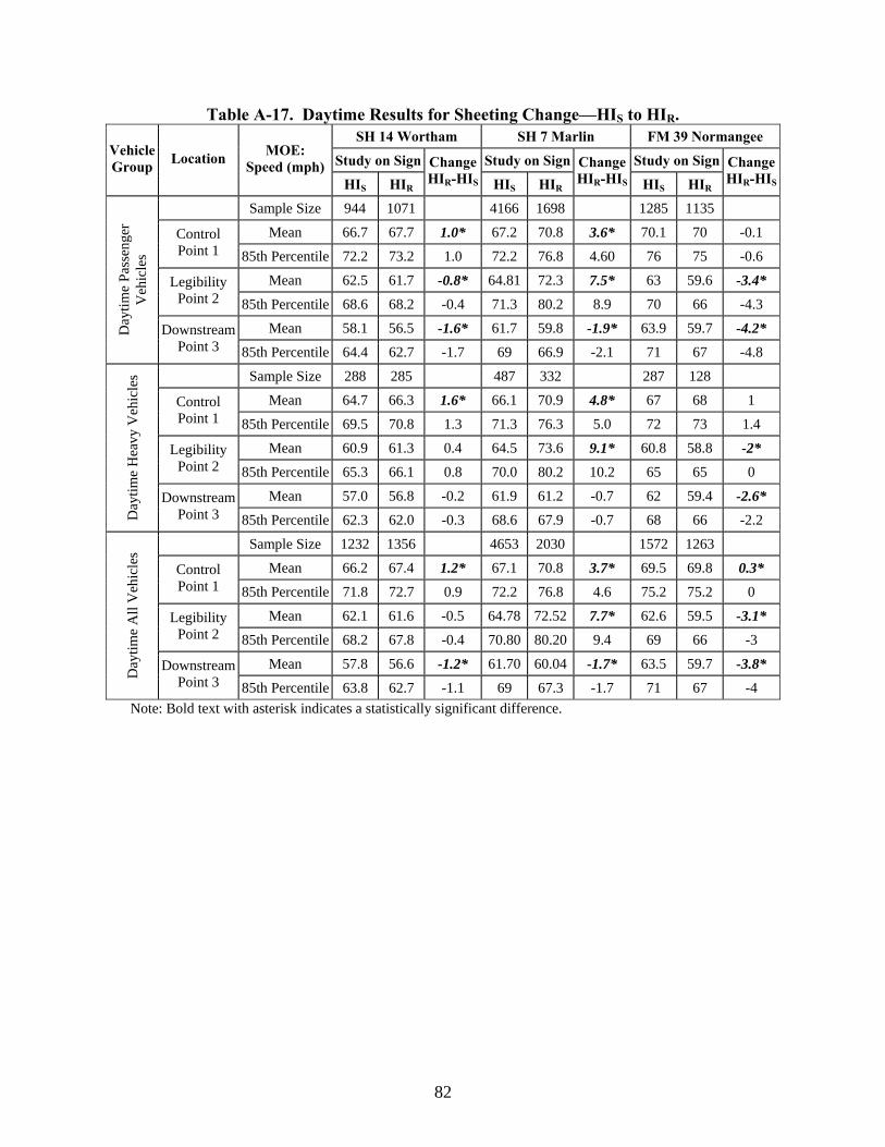
82

Table A-17. Daytime Results for Sheeting Change—HIS to HIR. SH 14 Wortham SH 7 Marlin FM 39 Normangee

Study on Sign Study on Sign Study on SignVehicle Group Location MOE:

Speed (mph) HIS HIR

ChangeHIR-HIS HIS HIR

Change HIR-HIS HIS HIR

ChangeHIR-HIS

Sample Size 944 1071 4166 1698 1285 1135

Mean 66.7 67.7 1.0* 67.2 70.8 3.6* 70.1 70 -0.1 Control Point 1 85th Percentile 72.2 73.2 1.0 72.2 76.8 4.60 76 75 -0.6

Mean 62.5 61.7 -0.8* 64.81 72.3 7.5* 63 59.6 -3.4* Legibility Point 2 85th Percentile 68.6 68.2 -0.4 71.3 80.2 8.9 70 66 -4.3

Mean 58.1 56.5 -1.6* 61.7 59.8 -1.9* 63.9 59.7 -4.2* Day

time

Pass

enge

r V

ehic

les

Downstream Point 3 85th Percentile 64.4 62.7 -1.7 69 66.9 -2.1 71 67 -4.8

Sample Size 288 285 487 332 287 128

Mean 64.7 66.3 1.6* 66.1 70.9 4.8* 67 68 1 Control Point 1 85th Percentile 69.5 70.8 1.3 71.3 76.3 5.0 72 73 1.4

Mean 60.9 61.3 0.4 64.5 73.6 9.1* 60.8 58.8 -2* Legibility Point 2 85th Percentile 65.3 66.1 0.8 70.0 80.2 10.2 65 65 0

Mean 57.0 56.8 -0.2 61.9 61.2 -0.7 62 59.4 -2.6*

Day

time

Hea

vy V

ehic

les

Downstream Point 3 85th Percentile 62.3 62.0 -0.3 68.6 67.9 -0.7 68 66 -2.2

Sample Size 1232 1356 4653 2030 1572 1263

Mean 66.2 67.4 1.2* 67.1 70.8 3.7* 69.5 69.8 0.3* Control Point 1 85th Percentile 71.8 72.7 0.9 72.2 76.8 4.6 75.2 75.2 0

Mean 62.1 61.6 -0.5 64.78 72.52 7.7* 62.6 59.5 -3.1* Legibility Point 2 85th Percentile 68.2 67.8 -0.4 70.80 80.20 9.4 69 66 -3

Mean 57.8 56.6 -1.2* 61.70 60.04 -1.7* 63.5 59.7 -3.8*

Day

time

All

Veh

icle

s

Downstream Point 3 85th Percentile 63.8 62.7 -1.1 69 67.3 -1.7 71 67 -4


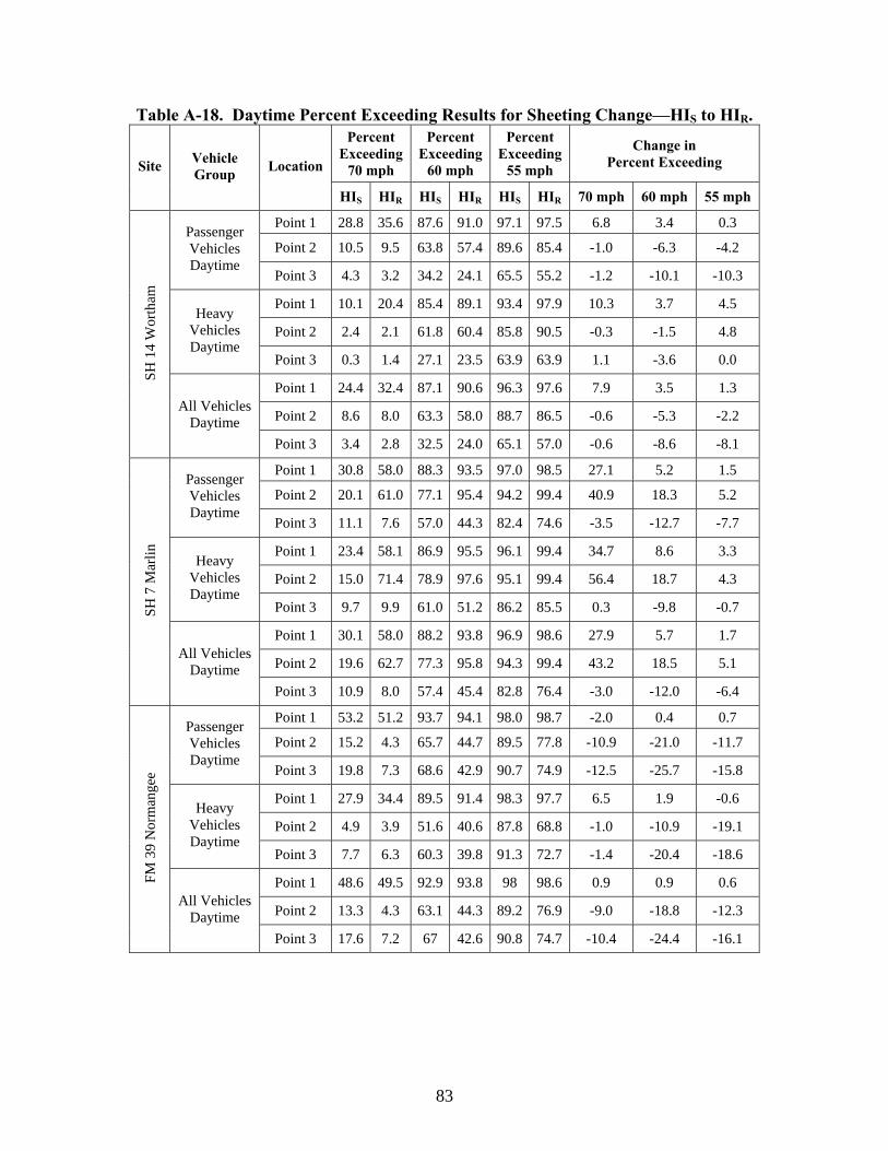
83

Table A-18. Daytime Percent Exceeding Results for Sheeting Change—HIS to HIR. Percent

Exceeding70 mph

Percent Exceeding

60 mph

Percent Exceeding

55 mph


Group Location

HIS HIR HIS HIR HIS HIR 70 mph 60 mph 55 mph

Point 1 28.8 35.6 87.6 91.0 97.1 97.5 6.8 3.4 0.3


Point 3 4.3 3.2 34.2 24.1 65.5 55.2 -1.2 -10.1 -10.3

Point 1 10.1 20.4 85.4 89.1 93.4 97.9 10.3 3.7 4.5

Point 2 2.4 2.1 61.8 60.4 85.8 90.5 -0.3 -1.5 4.8 Heavy

Vehicles Daytime

Point 3 0.3 1.4 27.1 23.5 63.9 63.9 1.1 -3.6 0.0

Point 1 24.4 32.4 87.1 90.6 96.3 97.6 7.9 3.5 1.3

Point 2 8.6 8.0 63.3 58.0 88.7 86.5 -0.6 -5.3 -2.2

SH 1

4 W

orth

am


Point 3 3.4 2.8 32.5 24.0 65.1 57.0 -0.6 -8.6 -8.1

Point 1 30.8 58.0 88.3 93.5 97.0 98.5 27.1 5.2 1.5


Point 3 11.1 7.6 57.0 44.3 82.4 74.6 -3.5 -12.7 -7.7

Point 1 23.4 58.1 86.9 95.5 96.1 99.4 34.7 8.6 3.3

Point 2 15.0 71.4 78.9 97.6 95.1 99.4 56.4 18.7 4.3 Heavy

Vehicles Daytime

Point 3 9.7 9.9 61.0 51.2 86.2 85.5 0.3 -9.8 -0.7

Point 1 30.1 58.0 88.2 93.8 96.9 98.6 27.9 5.7 1.7

Point 2 19.6 62.7 77.3 95.8 94.3 99.4 43.2 18.5 5.1

SH 7

Mar

lin


Point 3 10.9 8.0 57.4 45.4 82.8 76.4 -3.0 -12.0 -6.4

Point 1 53.2 51.2 93.7 94.1 98.0 98.7 -2.0 0.4 0.7


Point 3 19.8 7.3 68.6 42.9 90.7 74.9 -12.5 -25.7 -15.8

Point 1 27.9 34.4 89.5 91.4 98.3 97.7 6.5 1.9 -0.6

Point 2 4.9 3.9 51.6 40.6 87.8 68.8 -1.0 -10.9 -19.1 Heavy

Vehicles Daytime

Point 3 7.7 6.3 60.3 39.8 91.3 72.7 -1.4 -20.4 -18.6

Point 1 48.6 49.5 92.9 93.8 98 98.6 0.9 0.9 0.6

Point 2 13.3 4.3 63.1 44.3 89.2 76.9 -9.0 -18.8 -12.3

FM 3

9 N

orm

ange

e


Point 3 17.6 7.2 67 42.6 90.8 74.7 -10.4 -24.4 -16.1

84

Table A-19. Nighttime Results for Sheeting Change—HIS to HIR. SH 14 Wortham SH 7 Marlin FM 39 Normangee

Study on Sign Study on Sign Study on SignVehicle Group Location MOE:

Speed (mph) HIS HIR

ChangeHIR-HIS HIS HIR

Change HIR-HIS HIS HIR

ChangeHIR-HIS

Sample Size 402 275 2025 376 236 221

Mean 63.8 64.6 0.8 64.7 68.5 3.8* 69.1 68 -1.1 Control Point 1 85th Percentile 69.0 70.4 1.4 69.9 74.7 4.8 75 74 -1

Mean 59.0 59.3 0.3 61.5 69.3 7.8* 61.4 57.9 -3.5* Legibility Point 2 85th Percentile 65.7 66.1 0.4 67.8 77.4 9.6 67 65 -2.7

Mean 55.1 54.8 -0.3 58.5 57.8 -0.8 62.1 57.8 -4.3* Nig

httim

e Pa

ssen

ger

Veh

icle

s

Downstream Point 3 85th Percentile 61.3 60.6 -0.7 65.3 65.7 0.4 69 65 -3.7

Sample Size 105 75 250 95 101 47

Mean 62.9 64.3 1.5 64.8 68.7 3.9* 66.8 66.2 -0.6 Control Point 1 85th Percentile 67.3 68.5 1.2 69.3 73.2 3.9 71 71 -0.2

Mean 59.1 59.8 0.8 61.7 70.6 8.9* 60.9 58.1 -2.8* Legibility Point 2 85th Percentile 64.0 66.4 2.5 66.1 76.3 10.2 66 62 -3.6

Mean 55.0 55.7 0.7 58.9 58.9 0.1 62.1 57.9 -4.2*

Nig

httim

e H

eavy

Veh

icle

s

Downstream Point 3 85th Percentile 59.2 61.3 2.1 64.9 64.2 -0.7 69 63 -5.8

Sample Size 507 350 2275 471 337 268

Mean 63.6 64.5 0.9* 64.7 68.6 3.8* 68.4 67.7 -0.7 Control Point 1 85th Percentile 68.6 70.4 1.8 69.5 74.2 4.7 75 74 -1

Mean 59.0 59.4 0.4 61.6 69.6 8.0* 61.2 58 -3.2* Legibility Point 2 85th Percentile 65.3 66.1 0.8 67.3 77.4 10.1 67 64 -3

Mean 55.1 55.0 -0.1 58.6 58.0 -0.6 62.1 57.8 -4.3*

Nig

httim

e A

ll V

ehic

les

Downstream Point 3 85th Percentile 60.9 61.2 0.2 65.3 65.3 0.0 69 65 -4


85

Table A-20. Nighttime Percent Exceeding Results for Sheeting Change—HIS to HIR. Percent

Exceeding65 mph

Percent Exceeding

60 mph

Percent Exceeding

55 mph


Group Location

HIS HIR HIS HIR HIS HIR 65 mph 60 mph 55 mph Point 1 39.3 44.0 74.6 79.6 94.8 93.5 4.7 5.0 -1.3 Point 2 17.2 17.5 39.1 44.4 70.4 71.3 0.3 5.3 0.9

Passenger Vehicles

Nighttime Point 3 6.7 7.6 18.7 18.5 43.3 41.1 0.9 -0.1 -2.2 Point 1 37.1 46.7 74.3 76.0 91.4 97.3 9.5 1.7 5.9 Point 2 11.4 20.0 39.0 40.0 74.3 84.0 8.6 1.0 9.7

Heavy Vehicles

Nighttime Point 3 4.8 8.0 13.3 20.0 41.9 46.7 3.2 6.7 4.8 Point 1 38.9 44.6 74.6 78.9 94.1 94.3 5.7 4.3 0.2 Point 2 16.0 18.0 39.1 43.4 71.2 74.0 2.0 4.4 2.8

SH 1

4 W

orth

am


Point 3 6.3 7.7 17.6 18.9 43.0 42.3 1.4 1.3 -0.7 Point 1 47.4 70.2 80.7 87.8 95.5 96.3 22.9 7.0 0.8 Point 2 27.7 68.9 57.9 87.5 84.0 96.3 41.2 29.6 12.3

Passenger Vehicles

Nighttime Point 3 15.8 16.5 36.4 32.2 68.1 59.0 0.7 -4.3 -9.1 Point 1 46.0 81.1 84.8 95.8 96.4 98.9 35.1 11.0 2.5 Point 2 24.8 78.9 64.0 94.7 87.2 98.9 54.1 30.7 11.7

Heavy Vehicles

Nighttime Point 3 12.8 10.5 41.6 41.1 73.6 75.8 -2.3 -0.5 2.2 Point 1 47.2 72.4 81.2 89.4 95.6 96.8 25.2 8.2 1.3 Point 2 27.3 70.9 58.6 89.0 84.4 96.8 43.6 30.4 12.5

SH 7

Mar

lin


Point 3 15.4 15.3 37.0 34.0 68.7 62.4 -0.1 -3.0 -6.3 Point 1 76.3 71.0 94.5 89.6 99.2 97.3 -5.2 -4.9 -1.9 Point 2 27.5 11.8 55.5 34.8 85.6 67.4 -15.8 -20.7 -18.2

Passenger Vehicles

Nighttime Point 3 27.1 13.6 58.5 32.1 87.3 63.3 -13.5 -26.3 -23.9 Point 1 66.3 53.2 94.1 89.4 100.0 100.0 -13.1 -4.7 0.0 Point 2 26.7 6.4 48.5 31.9 88.1 72.3 -20.3 -16.6 -15.8

Heavy Vehicles

Nighttime Point 3 28.7 8.5 59.4 29.8 92.1 76.6 -20.2 -29.6 -15.5 Point 1 73.3 67.9 94.4 89.6 99.4 97.8 -5.4 -4.8 -1.6 Point 2 27.3 10.8 53.4 34.3 86.4 68.3 -16.5 -19.1 -18.1

FM 3

9 N

orm

ange

e


Point 3 27.6 12.7 58.8 31.7 88.7 65.7 -14.9 -27.1 -23.0

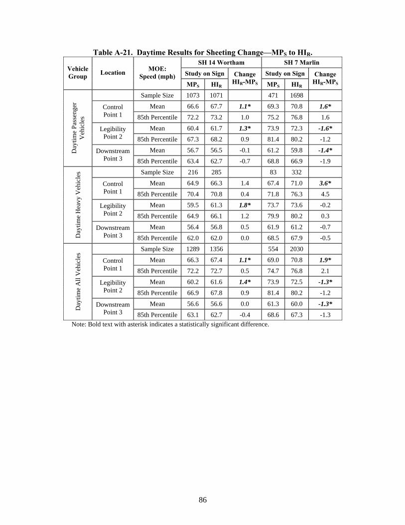
86

Table A-21. Daytime Results for Sheeting Change—MPS to HIR. SH 14 Wortham SH 7 Marlin


Speed (mph) MPS HIR

Change HIR-MPS MPS HIR

Change HIR-MPS

Sample Size 1073 1071 471 1698

Mean 66.6 67.7 1.1* 69.3 70.8 1.6* Control Point 1 85th Percentile 72.2 73.2 1.0 75.2 76.8 1.6

Mean 60.4 61.7 1.3* 73.9 72.3 -1.6* Legibility Point 2 85th Percentile 67.3 68.2 0.9 81.4 80.2 -1.2

Mean 56.7 56.5 -0.1 61.2 59.8 -1.4* Day

time

Pass

enge

r V

ehic

les


Sample Size 216 285 83 332


Mean 59.5 61.3 1.8* 73.7 73.6 -0.2 Legibility Point 2 85th Percentile 64.9 66.1 1.2 79.9 80.2 0.3

Mean 56.4 56.8 0.5 61.9 61.2 -0.7

Day

time

Hea

vy V

ehic

les

Downstream Point 3 85th Percentile 62.0 62.0 0.0 68.5 67.9 -0.5

Sample Size 1289 1356 554 2030

Mean 66.3 67.4 1.1* 69.0 70.8 1.9* Control Point 1 85th Percentile 72.2 72.7 0.5 74.7 76.8 2.1

Mean 60.2 61.6 1.4* 73.9 72.5 -1.3* Legibility Point 2 85th Percentile 66.9 67.8 0.9 81.4 80.2 -1.2

Mean 56.6 56.6 0.0 61.3 60.0 -1.3*

Day

time

All

Veh

icle

s



87

Table A-22. Daytime Percent Exceeding Results for Sheeting Change—MPS to HIR. Percent

Exceeding70 mph

Percent Exceeding

60 mph

Percent Exceeding

55 mph


Group Location

MPS HIR MPS HIR MPS HIR 70 mph 60 mph 55 mph

Point 1 27.8 35.6 85.0 91.0 96.6 97.5 7.8 6.0 0.9


Point 3 3.0 3.2 27.3 24.1 54.8 55.2 0.2 -3.2 0.4

Point 1 16.7 20.4 83.8 89.1 96.8 97.9 3.7 5.3 1.1

Point 2 2.3 2.1 44.0 60.4 79.2 90.5 -0.2 16.4 11.4 Heavy

Vehicles Daytime

Point 3 0.0 1.4 26.9 23.5 57.9 63.9 1.4 -3.3 6.0

Point 1 25.9 32.4 84.8 90.6 96.6 97.6 6.5 5.8 1.0

Point 2 5.4 8.0 50.8 58.0 77.8 86.5 2.6 7.2 8.7

SH 1

4 W

orth

am


Point 3 2.5 2.8 27.2 24.0 55.3 57.0 0.3 -3.3 1.7

Point 1 47.1 58.0 91.7 93.5 97.7 98.5 10.8 1.8 0.8


Point 3 11.7 7.6 54.1 44.3 78.8 74.6 -4.1 -9.9 -4.2

Point 1 27.7 58.1 90.4 95.5 98.8 99.4 30.4 5.1 0.6

Point 2 72.3 71.4 98.8 97.6 100.0 99.4 -0.9 -1.2 -0.6 Heavy

Vehicles Daytime

Point 3 7.2 9.9 59.0 51.2 90.4 85.5 2.7 -7.8 -4.8

Point 1 44.2 58.0 91.5 93.8 97.8 98.6 13.8 2.3 0.8

Point 2 69.7 62.7 97.5 95.8 99.8 99.4 -7.0 -1.7 -0.5

SH 7

Mar

lin


Point 3 11.0 8.0 54.9 45.4 80.5 76.4 -3.0 -9.5 -4.1

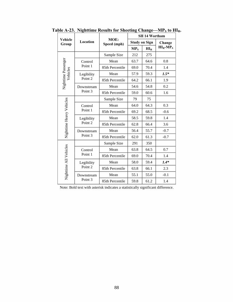
88

Table A-23. Nighttime Results for Sheeting Change—MPS to HIR. SH 14 Wortham

Study on Sign Vehicle Group Location MOE:

Speed (mph) MPS HIR

Change HIR-MPS

Sample Size 212 275


Mean 57.9 59.3 1.5* Legibility Point 2 85th Percentile 64.2 66.1 1.9

Mean 54.6 54.8 0.2 Nig

httim

e Pa

ssen

ger

Veh

icle

s


Sample Size 79 75

Mean 64.0 64.3 0.3 Control Point 1 85th Percentile 69.2 68.5 -0.6

Mean 58.5 59.8 1.4 Legibility Point 2 85th Percentile 62.8 66.4 3.6

Mean 56.4 55.7 -0.7

Nig

httim

e H

eavy

Veh

icle

s


Sample Size 291 350


Mean 58.0 59.4 1.4* Legibility Point 2 85th Percentile 63.8 66.1 2.3

Mean 55.1 55.0 -0.1

Nig

httim

e A

ll V

ehic

les



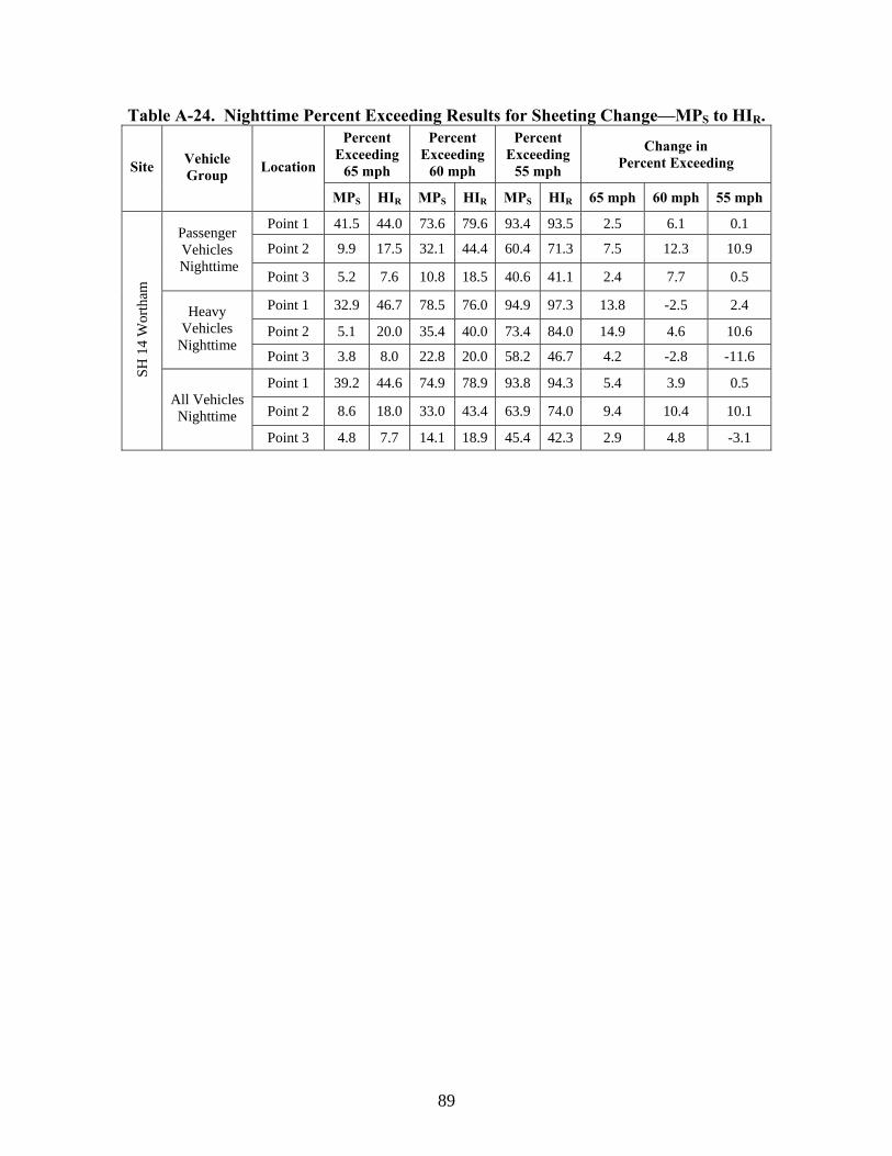
89

Table A-24. Nighttime Percent Exceeding Results for Sheeting Change—MPS to HIR. Percent

Exceeding65 mph

Percent Exceeding

60 mph

Percent Exceeding

55 mph


Group Location

MPS HIR MPS HIR MPS HIR 65 mph 60 mph 55 mph

Point 1 41.5 44.0 73.6 79.6 93.4 93.5 2.5 6.1 0.1

Point 2 9.9 17.5 32.1 44.4 60.4 71.3 7.5 12.3 10.9 Passenger Vehicles

Nighttime Point 3 5.2 7.6 10.8 18.5 40.6 41.1 2.4 7.7 0.5

Point 1 32.9 46.7 78.5 76.0 94.9 97.3 13.8 -2.5 2.4

Point 2 5.1 20.0 35.4 40.0 73.4 84.0 14.9 4.6 10.6 Heavy

Vehicles Nighttime

Point 3 3.8 8.0 22.8 20.0 58.2 46.7 4.2 -2.8 -11.6

Point 1 39.2 44.6 74.9 78.9 93.8 94.3 5.4 3.9 0.5

Point 2 8.6 18.0 33.0 43.4 63.9 74.0 9.4 10.4 10.1

SH 1

4 W

orth

am


Point 3 4.8 7.7 14.1 18.9 45.4 42.3 2.9 4.8 -3.1

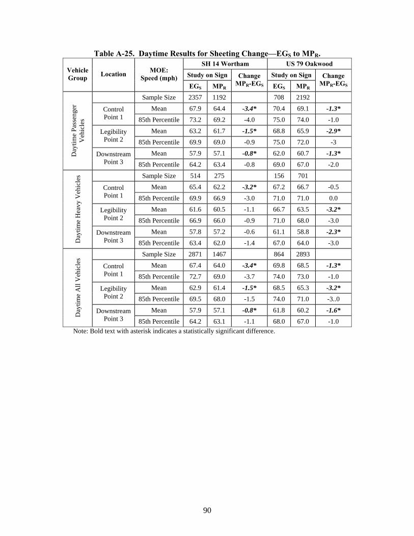
90

Table A-25. Daytime Results for Sheeting Change—EGS to MPR. SH 14 Wortham US 79 Oakwood


Speed (mph) EGS MPR

Change MPR-EGS EGS MPR

Change MPR-EGS

Sample Size 2357 1192 708 2192

Mean 67.9 64.4 -3.4* 70.4 69.1 -1.3* Control Point 1 85th Percentile 73.2 69.2 -4.0 75.0 74.0 -1.0

Mean 63.2 61.7 -1.5* 68.8 65.9 -2.9* Legibility Point 2 85th Percentile 69.9 69.0 -0.9 75.0 72.0 -3

Mean 57.9 57.1 -0.8* 62.0 60.7 -1.3* Day

time

Pass

enge

r V

ehic

les


Sample Size 514 275 156 701

Mean 65.4 62.2 -3.2* 67.2 66.7 -0.5 Control Point 1 85th Percentile 69.9 66.9 -3.0 71.0 71.0 0.0

Mean 61.6 60.5 -1.1 66.7 63.5 -3.2* Legibility Point 2 85th Percentile 66.9 66.0 -0.9 71.0 68.0 -3.0

Mean 57.8 57.2 -0.6 61.1 58.8 -2.3*

Day

time

Hea

vy V

ehic

les


Sample Size 2871 1467 864 2893


Mean 62.9 61.4 -1.5* 68.5 65.3 -3.2* Legibility Point 2 85th Percentile 69.5 68.0 -1.5 74.0 71.0 -3..0

Mean 57.9 57.1 -0.8* 61.8 60.2 -1.6*

Day

time

All

Veh

icle

s



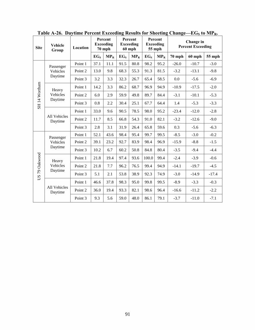
91

Table A-26. Daytime Percent Exceeding Results for Sheeting Change—EGS to MPR. Percent

Exceeding70 mph

Percent Exceeding

60 mph

Percent Exceeding

55 mph


Group Location

EGS MPR EGS MPR EGS MPR 70 mph 60 mph 55 mph

Point 1 37.1 11.1 91.5 80.8 98.2 95.2 -26.0 -10.7 -3.0


Point 3 3.2 3.3 32.3 26.7 65.4 58.5 0.0 -5.6 -6.9

Point 1 14.2 3.3 86.2 68.7 96.9 94.9 -10.9 -17.5 -2.0

Point 2 6.0 2.9 59.9 49.8 89.7 84.4 -3.1 -10.1 -5.3 Heavy

Vehicles Daytime

Point 3 0.8 2.2 30.4 25.1 67.7 64.4 1.4 -5.3 -3.3

Point 1 33.0 9.6 90.5 78.5 98.0 95.2 -23.4 -12.0 -2.8

Point 2 11.7 8.5 66.8 54.3 91.0 82.1 -3.2 -12.6 -9.0

SH 1

4 W

orth

am


Point 3 2.8 3.1 31.9 26.4 65.8 59.6 0.3 -5.6 -6.3

Point 1 52.1 43.6 98.4 95.4 99.7 99.5 -8.5 -3.0 -0.2


Point 3 10.2 6.7 60.2 50.8 84.8 80.4 -3.5 -9.4 -4.4

Point 1 21.8 19.4 97.4 93.6 100.0 99.4 -2.4 -3.9 -0.6

Point 2 21.8 7.7 96.2 76.5 99.4 94.9 -14.1 -19.7 -4.5 Heavy

Vehicles Daytime

Point 3 5.1 2.1 53.8 38.9 92.3 74.9 -3.0 -14.9 -17.4

Point 1 46.6 37.8 98.3 95.0 99.8 99.5 -8.9 -3.3 -0.3

Point 2 36.0 19.4 93.3 82.1 98.6 96.4 -16.6 -11.2 -2.2

US

79 O

akw

ood


Point 3 9.3 5.6 59.0 48.0 86.1 79.1 -3.7 -11.0 -7.1

92

Table A-27. Nighttime Results for Sheeting Change—EGS to MPR. SH 14 Wortham US 79 Oakwood


Speed (mph) EGS MPR

Change MPR-EGS EGS MPR

Change MPR-EGS

Sample Size 1562 217 387 505

Mean 65.2 61.7 -3.4* 68.0 67.4 -0.6 Control Point 1 85th Percentile 69.9 66.1 -3.8 72.0 72.0 0.0

Mean 60.4 57.7 -2.7* 67.6 65.2 -2.4* Legibility Point 2 85th Percentile 66.9 63.6 -3.3 74.0 71.0 -3.0

Mean 55.6 54.4 -1.2* 61.9 60.3 -1.6* Nig

httim

e Pa

ssen

ger

Veh

icle

s


Sample Size 414 85 103 284


Mean 59.6 59.1 -0.5 65.2 64.4 -0.8 Legibility Point 2 85th Percentile 64.9 65.0 0.1 69.0 69.0 0.0

Mean 55.3 55.7 0.4 59.2 59.5 0.3

Nig

httim

e H

eavy

Veh

icle

s


Sample Size 1976 302 490 789

Mean 64.9 61.4 -3.5* 67.5 66.9 -0.6 Control Point 1 85th Percentile 69.9 66.1 -3.8 72.0 71.0 -1.0


Mean 55.5 54.8 -0.7* 61.3 60 -1.3*

Nig

httim

e A

ll V

ehic

les



93

Table A-28. Nighttime Percent Exceeding Results for Sheeting Change—EGS to MPR. Percent

Exceeding65 mph

Percent Exceeding

60 mph

Percent Exceeding

55 mph


Group Location

EGS MPR EGS MPR EGS MPR 65 mph 60 mph 55 mph

Point 1 52.3 24.4 84.0 63.6 97.4 90.8 -27.9 -20.4 -6.6


Nighttime Point 3 7.6 3.2 21.3 13.4 48.3 38.2 -4.3 -7.9 -10.1

Point 1 39.6 5.9 77.3 57.6 93.7 90.6 -33.7 -19.6 -3.1

Point 2 13.8 8.2 44.7 43.5 78.3 70.6 -5.5 -1.2 -7.7 Heavy

Vehicles Nighttime

Point 3 5.1 3.5 16.2 16.5 48.8 49.4 -1.5 0.3 0.6

Point 1 49.6 19.2 82.6 61.9 96.6 90.7 -30.4 -20.7 -5.9

Point 2 20.0 9.9 48.6 34.4 80.5 63.6 -10.1 -14.2 -16.9

SH 1

4 W

orth

am


Point 3 7.0 3.3 20.2 14.2 48.4 41.4 -3.7 -6.0 -7.0

Point 1 72.4 66.3 97.4 91.3 99.7 98.0 -6.1 -6.1 -1.7


Nighttime Point 3 28.2 23.2 60.5 48.6 85.0 77.6 -5.0 -11.9 -7.4

Point 1 54.4 58.1 96.1 93.7 100.0 99.6 3.7 -2.5 -0.4

Point 2 54.4 44.4 90.3 79.9 98.1 97.2 -10.0 -10.4 -0.9 Heavy

Vehicles Nighttime

Point 3 12.6 14.4 42.7 42.6 77.7 77.8 1.8 -0.1 0.1

Point 1 68.6 63.4 97.1 92.1 99.8 99.1 -5.2 -5.0 -0.7

Point 2 64.5 48.9 89.4 78.8 98.6 95.2 -15.6 -10.6 -3.4

US

79 O

akw

ood


Point 3 24.9 20.0 56.7 46.4 83.5 77.7 -4.9 -10.3 -5.8

94

Table A-29. Daytime Results for Sheeting Change—HIS to MPR. SH 14 Wortham SH 7 Marlin


Speed (mph) HIS MPR

Change MPR-HIS HIS MPR

Change MPR-HIS

Sample Size 944 1192 4166 1714


Mean 62.5 61.7 -0.8* 64.8 69.5 4.7* Legibility Point 2 85th Percentile 68.6 69.0 0.4 71.3 76.0 4.7

Mean 58.1 57.1 -1.0* 61.7 60.8 -0.8* Day

time

Pass

enge

r V

ehic

les


Sample Size 288 275 487 269


Mean 60.9 60.5 -0.3 64.5 70.2 5.7* Legibility Point 2 85th Percentile 65.3 66.0 0.7 70.0 76.0 6.1

Mean 57.0 57.2 0.2 61.9 61.8 -0.1

Day

time

Hea

vy V

ehic

les


Sample Size 1232 1467 4653 1983



Mean 57.8 57.1 -0.7* 61.7 61.0 -0.7*

Day

time

All

Veh

icle

s



95

Table A-30. Daytime Percent Exceeding Results for Sheeting Change—HIS to MPR. Percent

Exceeding70 mph

Percent Exceeding

60 mph

Percent Exceeding

55 mph


Group Location

HIS MPR HIS MPR HIS MPR 70 mph 60 mph 55 mph

Point 1 28.8 11.1 87.6 80.8 97.1 95.2 -17.7 -6.8 -1.9


Point 3 4.3 3.3 34.2 26.7 65.5 58.5 -1.1 -7.5 -7.0

Point 1 10.1 3.3 85.4 68.7 93.4 94.9 -6.8 -16.7 1.5

Point 2 2.4 2.9 61.8 49.8 85.8 84.4 0.5 -12.0 -1.4 Heavy

Vehicles Daytime

Point 3 0.3 2.2 27.1 25.1 63.9 64.4 1.8 -2.0 0.5

Point 1 24.4 9.6 87.1 78.5 96.3 95.2 -14.8 -8.6 -1.1

Point 2 8.6 8.5 63.3 54.3 88.7 82.1 -0.1 -9.1 -6.6

SH 1

4 W

orth

am


Point 3 3.4 3.1 32.5 26.4 65.1 59.6 -0.3 -6.2 -5.5

Point 1 30.8 39.2 88.3 89.4 97.0 96.7 8.4 1.1 -0.3


Point 3 11.1 8.8 57.0 51.3 82.4 79.2 -2.3 -5.7 -3.1

Point 1 23.4 30.5 86.9 91.1 96.1 97.4 7.1 4.2 1.3

Point 2 15.0 48.7 78.9 94.4 95.1 99.3 33.7 15.6 4.2 Heavy

Vehicles Daytime

Point 3 9.7 11.2 61.0 56.9 86.2 86.6 1.5 -4.1 0.4

Point 1 30.1 38.0 88.2 89.7 96.9 96.8 8.0 1.5 -0.1

Point 2 19.6 45.1 77.3 91.3 94.3 98.4 25.6 14.0 4.1

SH 7

Mar

lin


Point 3 10.9 9.1 57.4 52.1 82.8 80.2 -1.9 -5.3 -2.5

96

Table A-31. Nighttime Results for Sheeting Change—HIS to MPR. SH 14 Wortham SH 7 Marlin


Speed (mph) HIS MPR

Change MPR-HIS HIS MPR

Change MPR-HIS

Sample Size 402 217 2025 366



Mean 55.1 54.4 -0.7 58.5 57.9 -0.6 Nig

httim

e Pa

ssen

ger

Veh

icle

s




Mean 59.1 59.1 0.0 61.7 67.1 5.4* Legibility Point 2 85th Percentile 64.0 65.0 1.0 66.1 72.0 5.9

Mean 55.0 55.7 0.7 58.9 59.5 0.6

Nig

httim

e H

eavy

Veh

icle

s


Sample Size 507 302 2275 464



Mean 55.1 54.8 -0.3 58.6 58.2 -0.4

Nig

httim

e A

ll V

ehic

les



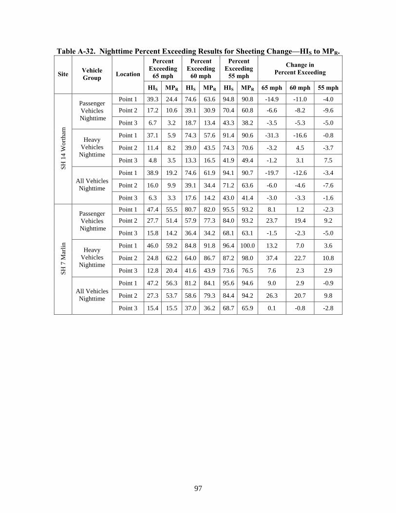
97

Table A-32. Nighttime Percent Exceeding Results for Sheeting Change—HIS to MPR. Percent

Exceeding65 mph

Percent Exceeding

60 mph

Percent Exceeding

55 mph


Group Location

HIS MPR HIS MPR HIS MPR 65 mph 60 mph 55 mph

Point 1 39.3 24.4 74.6 63.6 94.8 90.8 -14.9 -11.0 -4.0


Nighttime Point 3 6.7 3.2 18.7 13.4 43.3 38.2 -3.5 -5.3 -5.0

Point 1 37.1 5.9 74.3 57.6 91.4 90.6 -31.3 -16.6 -0.8

Point 2 11.4 8.2 39.0 43.5 74.3 70.6 -3.2 4.5 -3.7 Heavy

Vehicles Nighttime

Point 3 4.8 3.5 13.3 16.5 41.9 49.4 -1.2 3.1 7.5

Point 1 38.9 19.2 74.6 61.9 94.1 90.7 -19.7 -12.6 -3.4

Point 2 16.0 9.9 39.1 34.4 71.2 63.6 -6.0 -4.6 -7.6

SH 1

4 W

orth

am


Point 3 6.3 3.3 17.6 14.2 43.0 41.4 -3.0 -3.3 -1.6

Point 1 47.4 55.5 80.7 82.0 95.5 93.2 8.1 1.2 -2.3

Point 2 27.7 51.4 57.9 77.3 84.0 93.2 23.7 19.4 9.2 Passenger Vehicles

Nighttime Point 3 15.8 14.2 36.4 34.2 68.1 63.1 -1.5 -2.3 -5.0

Point 1 46.0 59.2 84.8 91.8 96.4 100.0 13.2 7.0 3.6

Point 2 24.8 62.2 64.0 86.7 87.2 98.0 37.4 22.7 10.8 Heavy

Vehicles Nighttime

Point 3 12.8 20.4 41.6 43.9 73.6 76.5 7.6 2.3 2.9

Point 1 47.2 56.3 81.2 84.1 95.6 94.6 9.0 2.9 -0.9

Point 2 27.3 53.7 58.6 79.3 84.4 94.2 26.3 20.7 9.8

SH 7

Mar

lin


Point 3 15.4 15.5 37.0 36.2 68.7 65.9 0.1 -0.8 -2.8

98

Table A-33. Daytime Results for Sheeting Change—MPS to MPR. SH 14 Wortham SH 7 Marlin US 79 Oakwood

Study on Sign Study on Sign Study on SignVehicle Group Location

MOE: Speed (mph) MPS MPR

Change MPR-MPS MPS MPR


Change MPR-MPS

Sample Size 1073 1192 471 1714 955 2192

Mean 66.6 64.4 -2.2* 69.3 67.9 -1.3* 69.7 69.1 -0.6* Control Point 1 85th

Percentile 72.2 69.2 -3.0 75.2 73.2 -2.0 74 74 0

Mean 60.4 61.7 1.3* 73.9 69.5 -4.4* 66 65.9 -0.1 Legibility

Point 2 85th Percentile 67.3 69.0 1.7 81.4 76.0 -5.4 72 72 0

Mean 56.7 57.1 0.4 61.2 60.8 -0.4 61.4 60.7 -0.7*

Day

time

Pass

enge

r Veh

icle

s

Downstream Point 3 85th

Percentile 63.4 63.4 0.0 68.8 68.2 -0.6 68 67 -1

Sample Size 216 275 83 269 347 701

Mean 64.9 62.2 -2.7* 67.4 67.3 0.1* 68.1 66.7 -1.4* Control Point 1 85th

Percentile 70.4 66.9 -3.5 71.8 73.1 1.3 72 71 -1

Mean 59.5 60.5 1.0 73.7 70.2 -3.5* 64.1 63.5 -0.6 Legibility

Point 2 85th Percentile 64.9 66.0 1.1 79.9 76.0 -3.9 69 68 -1

Mean 56.4 57.2 0.8 61.9 61.8 -0.1 60.1 58.8 -1.3* Day

time

Hea

vy V

ehic

les


Percentile 62.0 62.0 0.0 68.5 68.1 -0.4 65 64 -1

Sample Size 1289 1467 554 1983 1302 2893

Mean 66.3 64.0 -2.3* 69.0 67.9 -1.1* 69.3 68.5 -0.8* Control Point 1 85th

Percentile 72.2 69.0 -3.2 74.7 73.2 -1.5 74 73 -1

Mean 60.2 61.4 1.2* 73.9 69.6 -4.3* 65.5 65.3 -0.2 Legibility

Point 2 85th Percentile 66.9 68.0 1.1 81.4 76.0 -5.4 71 71 0

Mean 56.6 57.1 0.5 61.3 61.0 -0.3 61.1 60.2 -0.9* Day

time

All

Veh

icle

s


Percentile 63.1 63.1 0.0 68.6 68.2 -0.4 68 67 -1


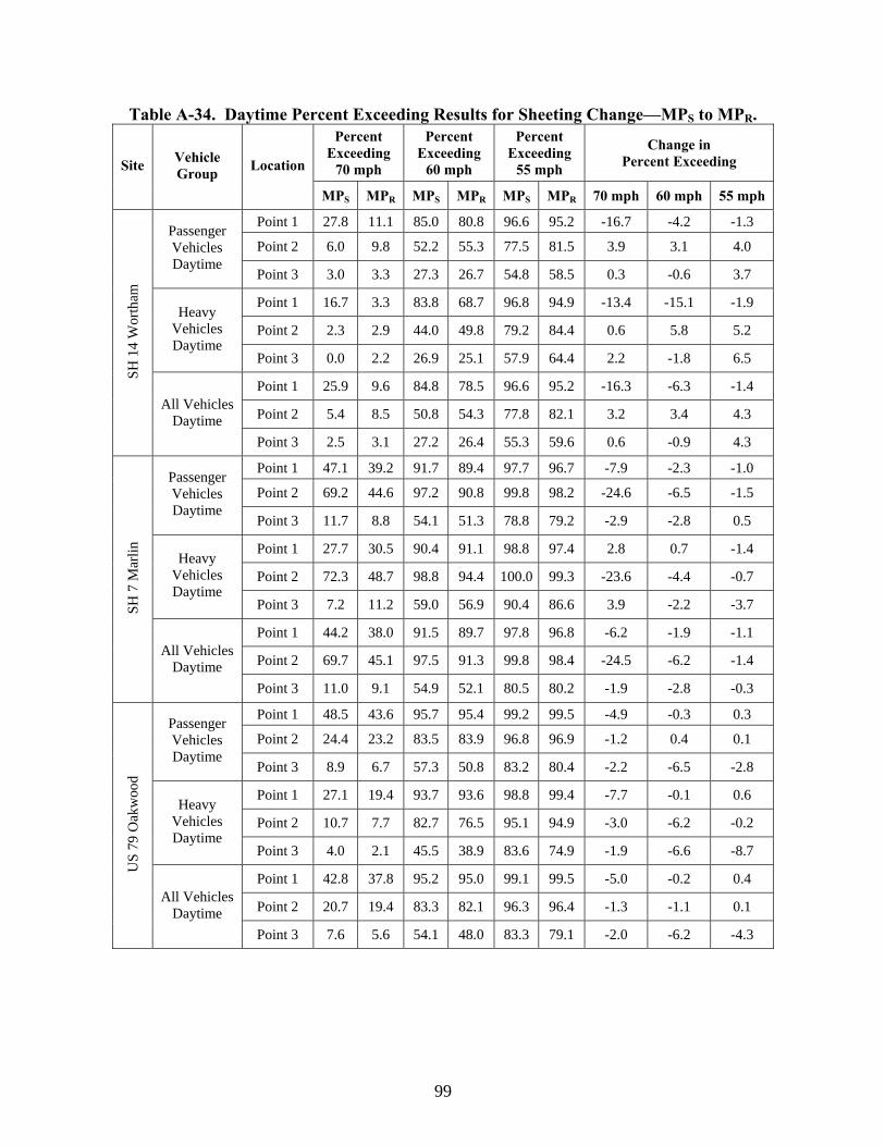
99

Table A-34. Daytime Percent Exceeding Results for Sheeting Change—MPS to MPR. Percent

Exceeding 70 mph

Percent Exceeding

60 mph

Percent Exceeding

55 mph


Group Location

MPS MPR MPS MPR MPS MPR 70 mph 60 mph 55 mph

Point 1 27.8 11.1 85.0 80.8 96.6 95.2 -16.7 -4.2 -1.3


Point 3 3.0 3.3 27.3 26.7 54.8 58.5 0.3 -0.6 3.7

Point 1 16.7 3.3 83.8 68.7 96.8 94.9 -13.4 -15.1 -1.9

Point 2 2.3 2.9 44.0 49.8 79.2 84.4 0.6 5.8 5.2 Heavy

Vehicles Daytime

Point 3 0.0 2.2 26.9 25.1 57.9 64.4 2.2 -1.8 6.5

Point 1 25.9 9.6 84.8 78.5 96.6 95.2 -16.3 -6.3 -1.4

Point 2 5.4 8.5 50.8 54.3 77.8 82.1 3.2 3.4 4.3

SH 1

4 W

orth

am


Point 3 2.5 3.1 27.2 26.4 55.3 59.6 0.6 -0.9 4.3

Point 1 47.1 39.2 91.7 89.4 97.7 96.7 -7.9 -2.3 -1.0


Point 3 11.7 8.8 54.1 51.3 78.8 79.2 -2.9 -2.8 0.5

Point 1 27.7 30.5 90.4 91.1 98.8 97.4 2.8 0.7 -1.4

Point 2 72.3 48.7 98.8 94.4 100.0 99.3 -23.6 -4.4 -0.7 Heavy

Vehicles Daytime

Point 3 7.2 11.2 59.0 56.9 90.4 86.6 3.9 -2.2 -3.7

Point 1 44.2 38.0 91.5 89.7 97.8 96.8 -6.2 -1.9 -1.1

Point 2 69.7 45.1 97.5 91.3 99.8 98.4 -24.5 -6.2 -1.4

SH 7

Mar

lin


Point 3 11.0 9.1 54.9 52.1 80.5 80.2 -1.9 -2.8 -0.3

Point 1 48.5 43.6 95.7 95.4 99.2 99.5 -4.9 -0.3 0.3

Point 2 24.4 23.2 83.5 83.9 96.8 96.9 -1.2 0.4 0.1 Passenger Vehicles Daytime

Point 3 8.9 6.7 57.3 50.8 83.2 80.4 -2.2 -6.5 -2.8

Point 1 27.1 19.4 93.7 93.6 98.8 99.4 -7.7 -0.1 0.6

Point 2 10.7 7.7 82.7 76.5 95.1 94.9 -3.0 -6.2 -0.2 Heavy

Vehicles Daytime

Point 3 4.0 2.1 45.5 38.9 83.6 74.9 -1.9 -6.6 -8.7

Point 1 42.8 37.8 95.2 95.0 99.1 99.5 -5.0 -0.2 0.4

Point 2 20.7 19.4 83.3 82.1 96.3 96.4 -1.3 -1.1 0.1

US

79 O

akw

ood


Point 3 7.6 5.6 54.1 48.0 83.3 79.1 -2.0 -6.2 -4.3

100

Table A-35. Nighttime Results for Sheeting Change—MPS to MPR. SH 14 Wortham US 79 Oakwood


Speed (mph) MPS MPR


Change MPR-MPS

Sample Size 212 217 267 505


Mean 57.9 57.7 -0.2 66 65.2 -0.8 Legibility Point 2 85th Percentile 64.2 63.6 -0.6 72.0 71.0 -1.0

Mean 54.6 54.4 -0.2 61.3 60.3 -1.0 Nig

httim

e Pa

ssen

ger

Veh

icle

s



Mean 64.0 60.5 -3.5* 67.2 66.2 -1.0 Control Point 1 85th Percentile 69.2 64.2 -5.0 71.0 70.0 -1.0

Mean 58.5 59.1 0.6 65.3 64.4 -0.9 Legibility Point 2 85th Percentile 62.8 65.0 2.2 70.0 69.0 -1.0

Mean 56.4 55.7 -0.8 60.9 59.5 -1.4

Nig

httim

e H

eavy

Veh

icle

s


Sample Size 291 302 401 789


Mean 58.0 58.1 0.0 65.8 64.9 -0.9* Legibility Point 2 85th Percentile 63.8 65.0 1.2 71.0 70.0 -1.0

Mean 55.1 54.8 -0.3 61.2 60 -1.2*

Nig

httim

e A

ll V

ehic

les



101

Table A-36. Nighttime Percent Exceeding Results for Sheeting Change—MPS to MPR. Percent

Exceeding 65 mph

Percent Exceeding

60 mph

Percent Exceeding

55 mph


Group Location

MPS MPR MPS MPR MPS MPR 65 mph 60 mph 55 mph

Point 1 41.5 24.4 73.6 63.6 93.4 90.8 -17.1 -10.0 -2.6

Point 2 9.9 10.6 32.1 30.9 60.4 60.8 0.7 -1.2 0.5 Passenger Vehicles

Nighttime Point 3 5.2 3.2 10.8 13.4 40.6 38.2 -2.0 2.5 -2.3

Point 1 32.9 5.9 78.5 57.6 94.9 90.6 -27.0 -20.8 -4.3

Point 2 5.1 8.2 35.4 43.5 73.4 70.6 3.2 8.1 -2.8 Heavy

Vehicles Nighttime

Point 3 3.8 3.5 22.8 16.5 58.2 49.4 -0.3 -6.3 -8.8

Point 1 39.2 19.2 74.9 61.9 93.8 90.7 -20.0 -13.0 -3.1

Point 2 8.6 9.9 33.0 34.4 63.9 63.6 1.3 1.4 -0.3

SH 1

4 W

orth

am


Point 3 4.8 3.3 14.1 14.2 45.4 41.4 -1.5 0.1 -4.0

Point 1 75.9 66.3 95.9 91.3 99.2 98.0 -9.6 -4.6 -1.2


Nighttime Point 3 30.5 23.2 53.8 48.6 82.0 77.6 -7.3 -5.2 -4.4

Point 1 61.9 58.1 93.3 93.7 100.0 99.6 -3.8 0.4 -0.4

Point 2 47.0 44.4 80.6 79.9 98.5 97.2 -2.6 -0.7 -1.3 Heavy

Vehicles Nighttime

Point 3 24.6 14.4 49.3 42.6 80.6 77.8 -10.2 -6.6 -2.8

Point 1 71.3 63.4 95.0 92.1 99.5 99.1 -8.0 -2.9 -0.4

Point 2 53.6 48.9 83.5 78.8 96.5 95.2 -4.7 -4.7 -1.3

US

79 O

akw

ood


Point 3 28.4 20.0 52.1 46.4 81.5 77.7 -8.4 -5.7 -3.9

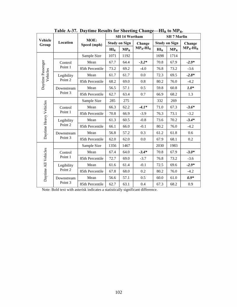
102

Table A-37. Daytime Results for Sheeting Change—HIR to MPR. SH 14 Wortham SH 7 Marlin


Speed (mph) HIR MPR

Change MPR-HIR HIR MPR

Change MPR-HIR

Sample Size 1071 1192 1698 1714


Mean 61.7 61.7 0.0 72.3 69.5 -2.8* Legibility Point 2 85th Percentile 68.2 69.0 0.8 80.2 76.0 -4.2

Mean 56.5 57.1 0.5 59.8 60.8 1.0* Day

time

Pass

enge

r V

ehic

les


Sample Size 285 275 332 269



Mean 56.8 57.2 0.3 61.2 61.8 0.6

Day

time

Hea

vy V

ehic

les


Sample Size 1356 1467 2030 1983


Mean 61.6 61.4 -0.1 72.5 69.6 -2.9* Legibility Point 2 85th Percentile 67.8 68.0 0.2 80.2 76.0 -4.2

Mean 56.6 57.1 0.5 60.0 61.0 0.9*

Day

time

All

Veh

icle

s



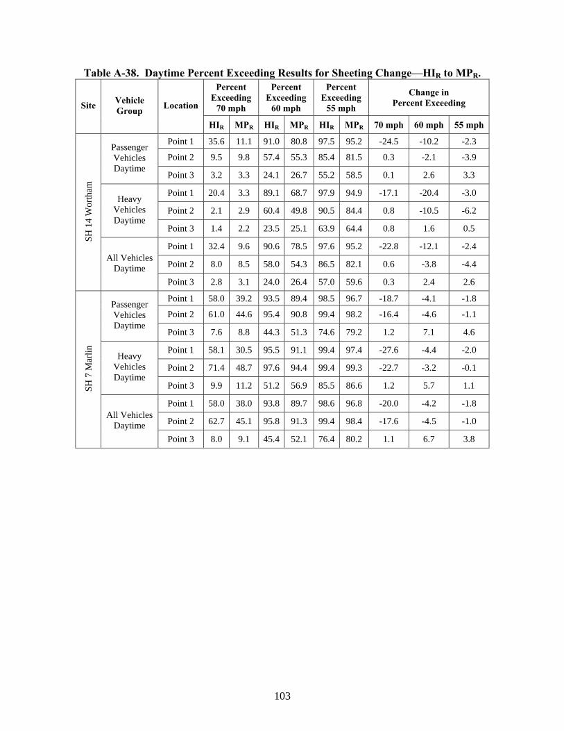
103

Table A-38. Daytime Percent Exceeding Results for Sheeting Change—HIR to MPR. Percent

Exceeding70 mph

Percent Exceeding

60 mph

Percent Exceeding

55 mph


Group Location

HIR MPR HIR MPR HIR MPR 70 mph 60 mph 55 mph

Point 1 35.6 11.1 91.0 80.8 97.5 95.2 -24.5 -10.2 -2.3

Point 2 9.5 9.8 57.4 55.3 85.4 81.5 0.3 -2.1 -3.9 Passenger Vehicles Daytime

Point 3 3.2 3.3 24.1 26.7 55.2 58.5 0.1 2.6 3.3

Point 1 20.4 3.3 89.1 68.7 97.9 94.9 -17.1 -20.4 -3.0

Point 2 2.1 2.9 60.4 49.8 90.5 84.4 0.8 -10.5 -6.2 Heavy

Vehicles Daytime

Point 3 1.4 2.2 23.5 25.1 63.9 64.4 0.8 1.6 0.5

Point 1 32.4 9.6 90.6 78.5 97.6 95.2 -22.8 -12.1 -2.4

Point 2 8.0 8.5 58.0 54.3 86.5 82.1 0.6 -3.8 -4.4

SH 1

4 W

orth

am


Point 3 2.8 3.1 24.0 26.4 57.0 59.6 0.3 2.4 2.6

Point 1 58.0 39.2 93.5 89.4 98.5 96.7 -18.7 -4.1 -1.8


Point 3 7.6 8.8 44.3 51.3 74.6 79.2 1.2 7.1 4.6

Point 1 58.1 30.5 95.5 91.1 99.4 97.4 -27.6 -4.4 -2.0

Point 2 71.4 48.7 97.6 94.4 99.4 99.3 -22.7 -3.2 -0.1 Heavy

Vehicles Daytime

Point 3 9.9 11.2 51.2 56.9 85.5 86.6 1.2 5.7 1.1

Point 1 58.0 38.0 93.8 89.7 98.6 96.8 -20.0 -4.2 -1.8

Point 2 62.7 45.1 95.8 91.3 99.4 98.4 -17.6 -4.5 -1.0

SH 7

Mar

lin


Point 3 8.0 9.1 45.4 52.1 76.4 80.2 1.1 6.7 3.8

104

Table A-39. Nighttime Results for Sheeting Change—HIR to MPR. SH 14 Wortham SH 7 Marlin


Speed (mph) HIR MPR

Change MPR-HIR HIR MPR

Change MPR-HIR

Sample Size 275 217 376 366



Mean 54.8 54.4 -0.4 57.8 57.9 0.1 Nig

httim

e Pa

ssen

ger

Veh

icle

s





Mean 55.7 55.7 0.0 59.0 59.5 0.5

Nig

httim

e H

eavy

Veh

icle

s


Sample Size 350 302 471 464



Mean 55.0 54.8 -0.2 58.0 58.2 0.2

Nig

httim

e A

ll V

ehic

les

Downstream

Point 3 85th Percentile 61.2 59.9 -1.3 65.3 65.3 0.0


105

Table A-40. Nighttime Percent Exceeding Results for Sheeting Change—HIR to MPR. Percent

Exceeding65 mph

Percent Exceeding

60 mph

Percent Exceeding

55 mph


Group Location

HIR MPR HIR MPR HIR MPR 65 mph 60 mph 55 mph

Point 1 44.0 24.4 79.6 63.6 93.5 90.8 -19.6 -16.0 -2.7


Nighttime Point 3 7.6 3.2 18.5 13.4 41.1 38.2 -4.4 -5.2 -2.8

Point 1 46.7 5.9 76.0 57.6 97.3 90.6 -40.8 -18.4 -6.7

Point 2 20.0 8.2 40.0 43.5 84.0 70.6 -11.8 3.5 -13.4 Heavy

Vehicles Nighttime

Point 3 8.0 3.5 20.0 16.5 46.7 49.4 -4.5 -3.5 2.7

Point 1 44.6 19.2 78.9 61.9 94.3 90.7 -25.4 -16.9 -3.6

Point 2 18.0 9.9 43.4 34.4 74.0 63.6 -8.1 -9.0 -10.4

SH 1

4 W

orth

am


Point 3 7.7 3.3 18.9 14.2 42.3 41.4 -4.4 -4.6 -0.9

Point 1 70.2 55.5 87.8 82.0 96.3 93.2 -14.7 -5.8 -3.1


Nighttime Point 3 16.5 14.2 32.2 34.2 59.0 63.1 -2.3 2.0 4.1

Point 1 81.1 59.2 95.8 91.8 98.9 100.0 -21.9 -4.0 1.1

Point 2 78.9 62.2 94.7 86.7 98.9 98.0 -16.7 -8.0 -1.0 Heavy

Vehicles Nighttime

Point 3 10.5 20.4 41.1 43.9 75.8 76.5 9.9 2.8 0.7

Point 1 72.4 56.3 89.4 84.1 96.8 94.6 -16.1 -5.3 -2.2

Point 2 70.9 53.7 89.0 79.3 96.8 94.2 -17.2 -9.6 -2.6

SH 7

Mar

lin


Point 3 15.3 15.5 34.0 36.2 62.4 65.9 0.2 2.2 3.5

107

APPENDIX B: LONG-TERM RED BORDER SPEED LIMIT SIGN RESULTS

The tables in this appendix present the results of the long-term analysis of the impacts of

the red border added to a standard Speed Limit sign. The researchers collected data at three sites

over the course of approximately one year. The before data were collected before the red border

was added to the existing sign. The short-term after data were collected within one month of the

installation of the red border. The long-term data were collected 9 to 12 months after the

installation of the red border.

108

Table B-1. Daytime Results for SH 21, All Vehicles.

Location MOE: Speed (mph) Before (B) Short-Term

After (STA) Long-TermAfter (LTA) STA-B LTA-B LTA-STA

Sample Size 1285 1182 3783

Mean 69 70.2 70 1.2* 1* -0.2

85th Percentile 74 75 75 1 1 0 Control Point 1

Std. Dev. 5.3 4.9 5.4

Mean 68.4 70.4 65.3 2* -3.1* -5.1* 85th Percentile 74 76 70 2 -4 -6

Threshold Point 2

Std. Dev. 5.8 5.9 5.2

Mean 64.2 64.7 0.5

85th Percentile 70 71 1 Legibility

Point 3 Std. Dev. 6.1 5.9

Mean 63.3 64.3 65.5 1* 2.2* 1.2*

85th Percentile 70 71 73 1 3 2 Sign

Point 4 Std. Dev. 6.4 6.5 6.9

Mean 63 62 59.7 -1* -3.3* -2.3*

85th Percentile 71 69 67 -2 -4 -2 Downstream

Point 5 Std. Dev. 6.8 6.6 7.3

Note: Asterisk (*) indicates a statistically significant difference between the compared speeds. Table B-2. Nighttime Results for SH 21, All Vehicles.



Sample Size 377 253 967

Mean 65.6 66.3 67.6 0.7 2* 1.3*


Std. Dev. 5.6 6.1 5.4

Mean 65 65.7 62.9 0.7 -2.1* -2.8* 85th Percentile 71 73 69 2 -2 -4

Threshold Point 2

Std. Dev. 6.4 6.6 5.4

Mean 60.1 62.3 2.2


Point 3 Std. Dev. 7.1 6 -1.1

Mean 60.1 60.5 63.4 0.4 3.3* 2.9* 85th Percentile 66 68 70 2 4 2

Sign Point 4

Std. Dev. 6.4 7.1 6.7 -0.4

Mean 60.2 58.4 58.6 -1.8* -1.6* 0.2


Point 5 Std. Dev. 6.7 6.9 7.5

Note: Asterisk (*) indicates a statistically significant difference between the compared speeds.

109

Table B-3. Daytime Results for SH 21, Passenger Vehicles.



Sample Size 1176 1075 3400

Mean 69.2 70.6 70.4 1.4* 1.2* -0.2


Std. Dev. 5.2 4.8 5.3

Mean 68.6 70.7 65.6 2.1* -3* -5.1* 85th Percentile 74 76 70

Threshold Point 2

Std. Dev. 5.8 5.9 5.2

Mean 64.5 65 0.5



Mean 63.5 64.7 65.7 1.2* 2.2* 1*


Point 4 Std. Dev. 6.4 6.5 6.9

Mean 63.1 62.3 59.8 -0.8* -3.3* -2.5*


Point 5 Std. Dev. 6.8 6.6 7.1

Note: Asterisk (*) indicates a statistically significant difference between the compared speeds. Table B-4. Daytime Results for SH 21, Heavy Vehicles.




Mean 66.1 66.3 66.6 0.2 0.5 0.3

85th Percentile 72 71 72 -1 0 1 Control Point 1

Std. Dev. 5.8 4.8 5.5

Mean 65.7 66.8 62.7 1.1 -3* -4.1* 85th Percentile 72 72 67 0 -5 -5

Threshold Point 2

Std. Dev. 5.9 4.9 5

Mean 60.9 62.2 1.3



Mean 61.1 61.2 63.2 0.1 2.1* 2* 85th Percentile 68 67 69 -1 1 2

Sign Point 4

Std. Dev. 6.2 5.7 6.1

Mean 61 59.3 58.4 -1.7 -2.6* -0.9


Point 5 Std. Dev. 6.7 5.3 8.8


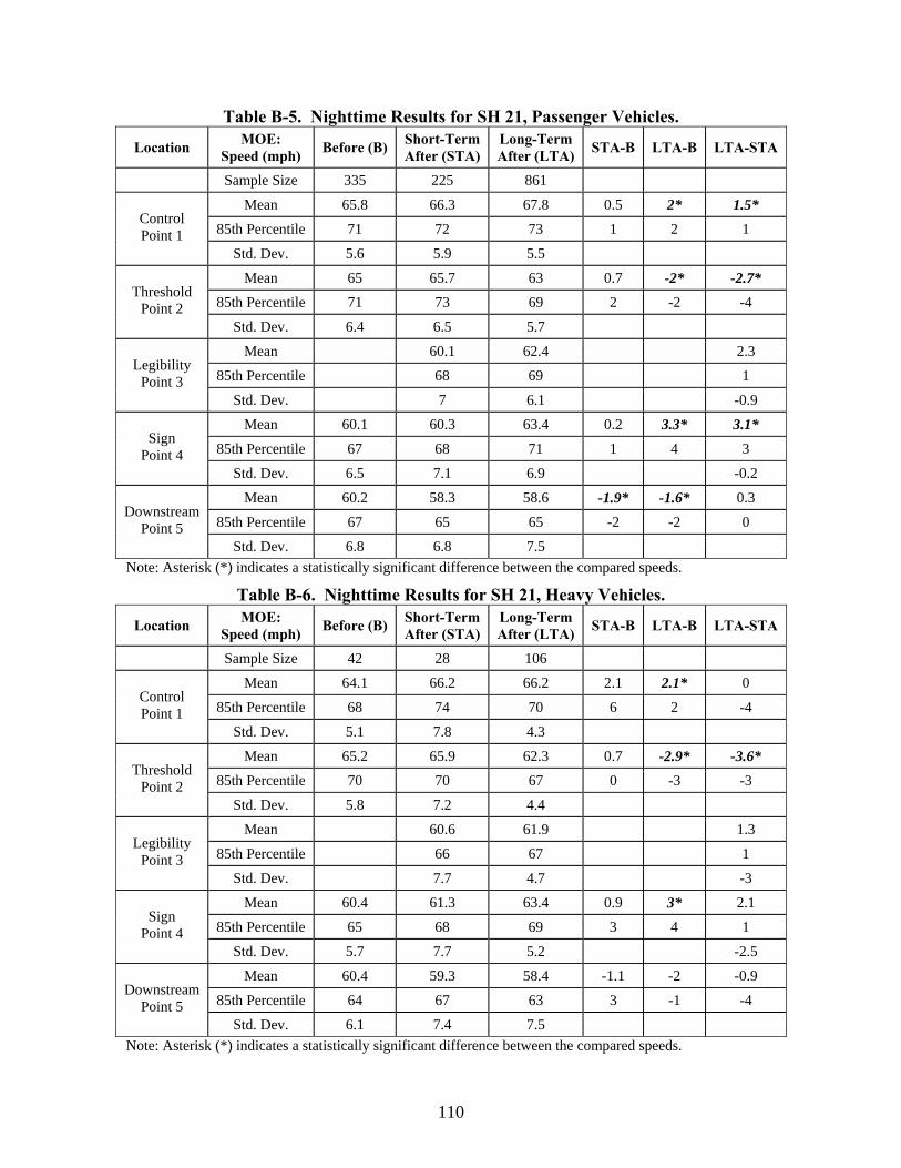
110

Table B-5. Nighttime Results for SH 21, Passenger Vehicles.




Mean 65.8 66.3 67.8 0.5 2* 1.5*


Std. Dev. 5.6 5.9 5.5

Mean 65 65.7 63 0.7 -2* -2.7* 85th Percentile 71 73 69 2 -2 -4

Threshold Point 2

Std. Dev. 6.4 6.5 5.7

Mean 60.1 62.4 2.3


Point 3 Std. Dev. 7 6.1 -0.9

Mean 60.1 60.3 63.4 0.2 3.3* 3.1*


Point 4 Std. Dev. 6.5 7.1 6.9 -0.2

Mean 60.2 58.3 58.6 -1.9* -1.6* 0.3

85th Percentile 67 65 65 -2 -2 0 Downstream

Point 5 Std. Dev. 6.8 6.8 7.5

Note: Asterisk (*) indicates a statistically significant difference between the compared speeds. Table B-6. Nighttime Results for SH 21, Heavy Vehicles.




Mean 64.1 66.2 66.2 2.1 2.1* 0

85th Percentile 68 74 70 6 2 -4 Control Point 1

Std. Dev. 5.1 7.8 4.3

Mean 65.2 65.9 62.3 0.7 -2.9* -3.6* 85th Percentile 70 70 67 0 -3 -3

Threshold Point 2

Std. Dev. 5.8 7.2 4.4

Mean 60.6 61.9 1.3


Point 3 Std. Dev. 7.7 4.7 -3

Mean 60.4 61.3 63.4 0.9 3* 2.1


Point 4 Std. Dev. 5.7 7.7 5.2 -2.5

Mean 60.4 59.3 58.4 -1.1 -2 -0.9

85th Percentile 64 67 63 3 -1 -4 Downstream

Point 5 Std. Dev. 6.1 7.4 7.5


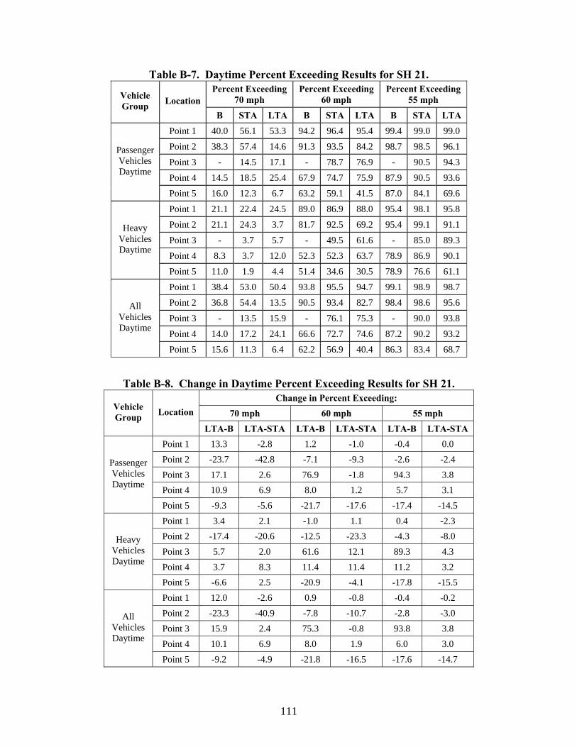
111

Table B-7. Daytime Percent Exceeding Results for SH 21. Percent Exceeding

70 mph Percent Exceeding


55 mph Vehicle Group Location

B STA LTA B STA LTA B STA LTA

Point 1 40.0 56.1 53.3 94.2 96.4 95.4 99.4 99.0 99.0

Point 2 38.3 57.4 14.6 91.3 93.5 84.2 98.7 98.5 96.1

Point 3 - 14.5 17.1 - 78.7 76.9 - 90.5 94.3

Point 4 14.5 18.5 25.4 67.9 74.7 75.9 87.9 90.5 93.6

Passenger Vehicles Daytime

Point 5 16.0 12.3 6.7 63.2 59.1 41.5 87.0 84.1 69.6

Point 1 21.1 22.4 24.5 89.0 86.9 88.0 95.4 98.1 95.8

Point 2 21.1 24.3 3.7 81.7 92.5 69.2 95.4 99.1 91.1

Point 3 - 3.7 5.7 - 49.5 61.6 - 85.0 89.3

Point 4 8.3 3.7 12.0 52.3 52.3 63.7 78.9 86.9 90.1

Heavy Vehicles Daytime

Point 5 11.0 1.9 4.4 51.4 34.6 30.5 78.9 76.6 61.1

Point 1 38.4 53.0 50.4 93.8 95.5 94.7 99.1 98.9 98.7

Point 2 36.8 54.4 13.5 90.5 93.4 82.7 98.4 98.6 95.6

Point 3 - 13.5 15.9 - 76.1 75.3 - 90.0 93.8

Point 4 14.0 17.2 24.1 66.6 72.7 74.6 87.2 90.2 93.2


Point 5 15.6 11.3 6.4 62.2 56.9 40.4 86.3 83.4 68.7

Table B-8. Change in Daytime Percent Exceeding Results for SH 21. Change in Percent Exceeding:

70 mph 60 mph 55 mph Vehicle Group Location

LTA-B LTA-STA LTA-B LTA-STA LTA-B LTA-STA Point 1 13.3 -2.8 1.2 -1.0 -0.4 0.0 Point 2 -23.7 -42.8 -7.1 -9.3 -2.6 -2.4 Point 3 17.1 2.6 76.9 -1.8 94.3 3.8 Point 4 10.9 6.9 8.0 1.2 5.7 3.1


Point 5 -9.3 -5.6 -21.7 -17.6 -17.4 -14.5 Point 1 3.4 2.1 -1.0 1.1 0.4 -2.3 Point 2 -17.4 -20.6 -12.5 -23.3 -4.3 -8.0 Point 3 5.7 2.0 61.6 12.1 89.3 4.3 Point 4 3.7 8.3 11.4 11.4 11.2 3.2


Point 5 -6.6 2.5 -20.9 -4.1 -17.8 -15.5 Point 1 12.0 -2.6 0.9 -0.8 -0.4 -0.2 Point 2 -23.3 -40.9 -7.8 -10.7 -2.8 -3.0 Point 3 15.9 2.4 75.3 -0.8 93.8 3.8 Point 4 10.1 6.9 8.0 1.9 6.0 3.0


Point 5 -9.2 -4.9 -21.8 -16.5 -17.6 -14.7

112

Table B-9. Nighttime Percent Exceeding Results for SH 21. Percent Exceeding





1 46.9 61.8 67.9 86.9 84.4 92.6 96.1 95.1 98.1

2 46.3 50.7 32.1 74.9 75.1 68.4 94.9 95.1 90.0

3 23.6 29.8 50.2 60.4 66.7 85.9

4 21.2 25.3 34.7 43.0 51.1 63.1 75.2 72.0 88.2

Passenger Vehicles

Nighttime

5 19.4 15.1 13.5 41.2 36.9 34.5 76.7 63.1 61.9

1 28.6 60.7 57.5 76.2 78.6 93.4 100.0 89.3 97.2

2 45.2 57.1 23.6 85.7 78.6 68.9 97.6 92.9 95.3

3 17.9 20.8 53.6 63.2 67.9 93.4

4 9.5 21.4 32.1 50.0 50.0 67.0 76.2 75.0 94.3

Heavy Vehicles

Nighttime

5 9.5 17.9 7.5 50.0 28.6 27.4 71.4 67.9 66.0

1 44.8 61.7 66.8 85.7 83.8 92.7 96.6 94.5 98.0

2 46.2 51.4 31.1 76.1 75.5 68.5 95.2 94.9 90.6

3 22.9 28.9 50.6 60.7 66.8 86.6

4 19.9 24.9 34.4 43.8 51.0 63.5 75.3 72.3 88.8

All Vehicles

Nighttime

5 18.3 15.4 12.8 42.2 36.0 33.7 76.1 63.3 62.4

Table B-10. Change in Nighttime Percent Exceeding Results for SH 21. Change in Percent Exceeding:


LTA-B LTA-STA LTA-B LTA-STA LTA-B LTA-STA Point 1 21.0 6.1 5.7 8.2 2.0 3.0 Point 2 -14.2 -18.6 -6.5 -6.7 -4.9 -5.1 Point 3 29.8 6.2 60.4 10.2 85.9 19.2 Point 4 13.5 9.4 20.1 12.0 13.0 16.2

Passenger Vehicles

Nighttime

Point 5 -5.9 -1.6 -6.7 -2.4 -14.8 -1.2 Point 1 28.9 -3.2 17.2 14.8 -2.8 7.9 Point 2 -21.6 -33.5 -16.8 -9.7 -2.3 2.4 Point 3 20.8 2.9 63.2 9.6 93.4 25.5 Point 4 22.6 10.7 17.0 17.0 18.1 19.3

Heavy Vehicles

Nighttime

Point 5 -2.0 -10.4 -22.6 -1.2 -5.4 -1.9 Point 1 22.0 5.1 7.0 8.9 1.4 3.5 Point 2 -15.1 -20.3 -7.6 -7.0 -4.6 -4.3 Point 3 28.9 6.0 60.7 10.1 86.6 19.8 Point 4 14.5 9.5 19.7 12.5 13.5 16.5

All Vehicles

Nighttime

Point 5 -5.5 -2.6 -8.5 -2.3 -13.7 -0.9

113

Table B-11. Daytime Results for FM 60, All Vehicles.




Mean 70.1 70.9 67.1 0.8 -3* -3.8*

85th Percentile 76 76 72 0 -4 -4 Control Point 1

Std. Dev. 5.8 5.6 5.7

Mean 68.3 67.7 63.2 -0.6 -5.1* -4.5* 85th Percentile 74 73 70 -1 -4 -3

Threshold Point 2

Std. Dev. 6.2 6.1 6

Mean 66.2 66.5 66.2 0.3 0 -0.3

85th Percentile 72 73 73 1 1 0 Legibility

Point 3 Std. Dev. 5.8 6 6.8

Mean 67.1 66.4 60.7 -0.7 -6.4* -5.7*

85th Percentile 73 73 67 0 -6 -6 Sign

Point 4 Std. Dev. 6.3 6.4 6.1

Mean 65 64.9 57.5 -0.1 -7.5* -7.4*


Point 5 Std. Dev. 6.3 6.5 5.7

Note: Asterisk (*) indicates a statistically significant difference between the compared speeds. Table B-12. Nighttime Results for FM 60, All Vehicles.




Mean 66.9 68.3 65.8 1.4* -1.1* -2.5*


Std. Dev. 5.8 6.1 6.2

Mean 63.4 63.1 61.1 -0.3 -2.3* -2* 85th Percentile 70 69 67.7 -1 -2.3 -1.3

Threshold Point 2

Std. Dev. 6.2 5.6 6.4

Mean 62.1 62.1 64 0 1.9* 1.9*


Point 3 Std. Dev. 6.3 5.7 7.3

Mean 62 61.5 58.8 -0.5 -3.2* -2.7* 85th Percentile 69 68 65 -1 -4 -3

Sign Point 4

Std. Dev. 6.6 6.1 6.7

Mean 60.8 60.2 56.2 -0.6 -4.6* -4*


Point 5 Std. Dev. 6.5 5.9 6.2


114

Table B-13. Daytime Results for FM 60, Passenger Vehicles.




Mean 70.3 70.8 67.5 0.5 -2.8* -3.3*


Std. Dev. 5.8 5.6 5.6

Mean 68.5 67.6 63.4 -0.9 -5.1* -4.2* 85th Percentile 75 73 70 -2 -5 -3

Threshold Point 2

Std. Dev. 6.2 6.1 6

Mean 66.3 66.4 66.4 0.1 0.1 0


Point 3 Std. Dev. 5.9 6.1 6.8

Mean 67.2 66.3 60.8 -0.9 -6.4* -5.5*


Point 4 Std. Dev. 6.3 6.4 6.1

Mean 65.1 64.7 57.6 -0.4 -7.5* -7.1*


Point 5 Std. Dev. 6.3 6.6 5.8

Note: Asterisk (*) indicates a statistically significant difference between the compared speeds. Table B-14. Daytime Results for FM 60, Heavy Vehicles.




Mean 68.6 71.9 64.2 3.3 -4.4* -7.7


Std. Dev. 5.7 5.2 5.7

Mean 67.2 70.3 61.5 3.1 -5.7* -8.8

85th Percentile 73 76 67 3 -6 -9 Threshold

Point 2 Std. Dev. 5.9 4.7 6

Mean 65.6 69.1 64.6 3.5 -1 -4.5

85th Percentile 71 75 71 4 0 -4 Legibility

Point 3 Std. Dev. 5.6 4.8 6.6

Mean 66.1 69.5 59.6 3.4 -6.5* -9.9


Point 4 Std. Dev. 6.4 5.5 5.5

Mean 64.5 68.2 56.6 3.7 -7.9* -11.6


Point 5 Std. Dev. 6.2 4.8 5.2


115

Table B-15. Nighttime Results for FM 60, Passeneger Vehicles.




Mean 67 68.6 65.9 1.6* -1.1* -2.7*


Std. Dev. 5.8 6.1 6.2

Mean 63.4 63.3 61.3 -0.1 -2.1* -2* 85th Percentile 70 69 68 -1 -2 -1

Threshold Point 2

Std. Dev. 6.3 5.6 6.4

Mean 62.2 62.2 64.1 0 1.9* 1.9*

85th Percentile 69 68 72 -1 3 4 Legibility

Point 3 Std. Dev. 6.3 5.8 7.3

Mean 62 61.6 58.9 -0.4 -3.1* -2.7*

85th Percentile 69 68 66 -1 -3.3 -2.3 Sign

Point 4 Std. Dev. 6.7 6.2 6.7

Mean 60.8 60.3 56.2 -0.5 -4.6* -4.1*



Note: Asterisk (*) indicates a statistically significant difference between the compared speeds. Table B-16. Nighttime Results for FM 60, Heavy Vehicles.




Mean 65.2 65.1 63 -0.1 -2.2 -2.1

85th Percentile 71 69 68 -2 -2.8 -0.8 Control Point 1

Std. Dev. 5.5 4.4 5.5

Mean 62.1 61.3 58.3 -0.8 -3.8* -3

85th Percentile 68 65 63 -3 -5 -2 Threshold

Point 2 Std. Dev. 4.9 4.7 5.1

Mean 60.7 60.5 60.8 -0.2 0.1 0.3

85th Percentile 67 64 66 -3 -1 2 Legibility

Point 3 Std. Dev. 5.2 4.4 5.8

Mean 60.3 60.3 56.5 0 -3.8* -3.8

85th Percentile 66 65 60 -1 -6 -5 Sign

Point 4 Std. Dev. 5.9 4.4 5

Mean 60 59.5 54.4 -0.5 -5.6* -5.1


Point 5 Std. Dev. 5.7 4.9 4.5


116

Table B-17. Daytime Percent Exceeding Results for FM 60. Percent Exceeding





Point 1 46.7 54.4 29.8 94.6 95.2 90.5 99.0 98.5 97.3

Point 2 36.3 32.7 12.2 90.0 86.5 71.2 97.6 96.1 91.3

Point 3 20.9 23.1 30.7 84.2 82.9 81.3 96.5 93.7 95.0

Point 4 28.5 24.3 5.6 85.4 80.8 54.0 96.7 93.7 81.8


Point 5 18.1 18.0 1.9 74.9 71.8 31.6 93.6 90.7 64.0

Point 1 32.7 62.5 15.3 89.3 100.0 78.9 99.4 100.0 93.2

Point 2 23.3 56.3 9.5 86.2 100.0 60.0 97.5 100.0 84.2

Point 3 15.7 43.8 19.5 79.9 100.0 75.8 96.2 100.0 89.5

Point 4 20.8 43.8 3.7 79.9 100.0 44.7 96.9 100.0 77.9


Point 5 14.5 37.5 1.1 73.6 100.0 24.2 91.8 100.0 62.1

Point 1 45.3 54.7 28.1 94.1 95.4 89.2 99.0 98.6 96.8

Point 2 35.0 33.8 11.9 89.6 87.1 69.9 97.6 96.3 90.5

Point 3 20.4 24.1 29.4 83.8 83.7 80.7 96.5 94.0 94.4

Point 4 27.7 25.2 5.4 84.8 81.7 52.9 96.7 94.0 81.4


Point 5 17.7 18.9 1.8 74.8 73.1 30.8 93.4 91.1 63.7

Table B-18. Change in Daytime Percent Exceeding Results for FM 60. Change in Percent Exceeding:


LTA-B LTA-STA LTA-B LTA-STA LTA-B LTA-STA Point 1 -16.9 -24.6 -4.1 -4.7 -1.7 -1.2 Point 2 -24.1 -20.5 -18.8 -15.3 -6.3 -4.8 Point 3 9.8 7.6 -2.9 -1.6 -1.5 1.3 Point 4 -22.9 -18.7 -31.4 -26.8 -14.9 -11.9


Point 5 -16.2 -16.1 -43.3 -40.2 -29.6 -26.7 Point 1 -17.4 -47.2 -10.4 -21.1 -6.2 -6.8 Point 2 -13.8 -46.8 -26.2 -40.0 -13.3 -15.8 Point 3 3.8 -24.3 -4.1 -24.2 -6.7 -10.5 Point 4 -17.1 -40.1 -35.2 -55.3 -19.0 -22.1


Point 5 -13.4 -36.4 -49.4 -75.8 -29.7 -37.9 Point 1 -17.2 -26.6 -4.9 -6.2 -2.2 -1.8 Point 2 -23.1 -21.9 -19.7 -17.2 -7.1 -5.8 Point 3 9.0 5.3 -3.1 -3.0 -2.1 0.4 Point 4 -22.3 -19.8 -31.9 -28.8 -15.3 -12.6


Point 5 -15.9 -17.1 -44.0 -42.3 -29.7 -27.4

117

Table B-19. Nighttime Percent Exceeding Results for FM 60. Percent Exceeding





Point 1 61.1 70.7 52.4 88.2 90.8 86.4 98.1 97.7 96.5

Point 2 35.5 38.5 25.6 65.3 67.2 55.3 90.5 89.7 84.6

Point 3 29.8 31.6 42.5 58.1 58.6 67.3 85.8 86.2 91.5

Point 4 32.8 28.2 17.6 56.0 55.2 39.6 81.0 81.6 68.6

Passenger Vehicles

Nighttime

Point 5 24.3 20.7 8.5 46.7 45.4 25.8 75.1 75.9 52.4

Point 1 52.0 53.3 31.3 80.0 80.0 71.9 100.0 100.0 93.8

Point 2 28.0 13.3 12.5 52.0 53.3 34.4 96.0 86.7 71.9

Point 3 20.0 13.3 21.9 52.0 46.7 50.0 76.0 93.3 87.5

Point 4 24.0 13.3 3.1 44.0 40.0 15.6 80.0 93.3 65.6

Heavy Vehicles

Nighttime

Point 5 16.0 13.3 3.1 44.0 33.3 9.4 80.0 80.0 46.9

Point 1 60.6 69.3 51.4 87.8 89.9 85.7 98.2 97.9 96.3

Point 2 35.1 36.5 25.0 64.7 66.1 54.3 90.8 89.4 84.0

Point 3 29.3 30.2 41.5 57.8 57.7 66.5 85.3 86.8 91.3

Point 4 32.3 27.0 16.9 55.4 54.0 38.4 80.9 82.5 68.4

All Vehicles

Nighttime

Point 5 23.9 20.1 8.2 46.6 44.4 25.0 75.3 76.2 52.1

Table B-20. Change in Nighttime Percent Exceeding Results for FM 60. Change in Percent Exceeding:


LTA-B LTA-STA LTA-B LTA-STA LTA-B LTA-STA Point 1 -8.7 -18.3 -1.8 -4.4 -1.6 -1.2 Point 2 -9.9 -12.9 -10.0 -11.9 -5.9 -5.1 Point 3 12.7 10.9 9.2 8.7 5.7 5.3 Point 4 -15.2 -10.6 -16.4 -15.6 -12.4 -13.0

Passenger Vehicles

Nighttime

Point 5 -15.8 -12.2 -20.9 -19.6 -22.7 -23.5 Point 1 -20.7 -22.0 -8.1 -8.1 -6.2 -6.2 Point 2 -15.5 -0.8 -17.6 -18.9 -24.1 -14.8 Point 3 1.9 8.6 -2.0 3.3 11.5 -5.8 Point 4 -20.9 -10.2 -28.4 -24.4 -14.4 -27.7

Heavy Vehicles

Nighttime

Point 5 -12.9 -10.2 -34.6 -23.9 -33.1 -33.1 Point 1 -9.2 -17.9 -2.1 -4.2 -1.9 -1.6 Point 2 -10.1 -11.5 -10.4 -11.8 -6.8 -5.4 Point 3 12.2 11.3 8.7 8.8 6.0 4.5 Point 4 -15.4 -10.1 -17.0 -15.6 -12.5 -14.1

All Vehicles

Nighttime

Point 5 -15.7 -11.9 -21.6 -19.4 -23.2 -24.1

118

Table B-21. Daytime Results for SH 36, All Vehicles.




Mean 70 72.1 71 2.1* 1* -1.1*


Std. Dev. 5.5 5.1 5.3

Mean 67.1 68.3 67.8 1.2* 0.7 -0.5

85th Percentile 73 73 73 0 0 0 Threshold

Point 2 Std. Dev. 6.1 5.2 5.7

Mean 66.8 67.7 66 0.9* -0.8* -1.7*

85th Percentile 73 73 72 0 -1 -1 Legibility

Point 3 Std. Dev. 6.1 5.7 5.9

Mean 65 65.4 66.5 0.4 1.5* 1.1*


Point 4 Std. Dev. 5.9 5.7 7.1

Mean 65 64.9 59.4 -0.1 -5.6* -5.5*


Point 5 Std. Dev. 6.3 6.1 6.2

Note: Asterisk (*) indicates a statistically significant difference between the compared speeds. Table B-22. Nighttime Results for SH 36, All Vehicles.




Mean 67.4 69.1 67.8 1.7 0.4 -1.3


Std. Dev. 4.8 5.7 5.2

Mean 63 64.3 64.3 1.3 1.3* 0


Point 2 Std. Dev. 5.6 5.5 5.9

Mean 62.9 63.9 63.1 1 0.2 -0.8


Point 3 Std. Dev. 5.4 5.7 5.8

Mean 61.2 61.8 64.3 0.6 3.1* 2.5* 85th Percentile 67 68 71 1 4 3

Sign Point 4

Std. Dev. 5.5 5.6 6.4

Mean 61.6 61.5 57.8 -0.1 -3.8* -3.7*


Point 5 Std. Dev. 5.8 5.3 5.5


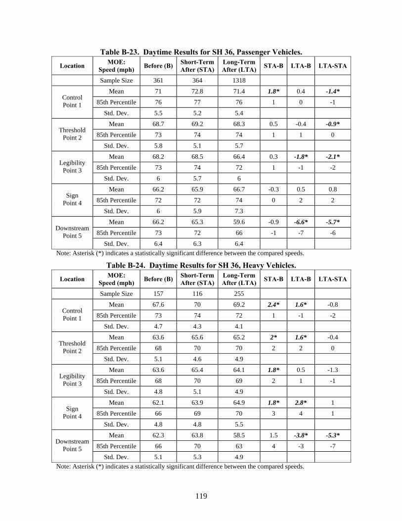
119

Table B-23. Daytime Results for SH 36, Passenger Vehicles.




Mean 71 72.8 71.4 1.8* 0.4 -1.4*


Std. Dev. 5.5 5.2 5.4

Mean 68.7 69.2 68.3 0.5 -0.4 -0.9* 85th Percentile 73 74 74 1 1 0

Threshold Point 2

Std. Dev. 5.8 5.1 5.7

Mean 68.2 68.5 66.4 0.3 -1.8* -2.1*


Point 3 Std. Dev. 6 5.7 6

Mean 66.2 65.9 66.7 -0.3 0.5 0.8


Point 4 Std. Dev. 6 5.9 7.3

Mean 66.2 65.3 59.6 -0.9 -6.6* -5.7*


Point 5 Std. Dev. 6.4 6.3 6.4

Note: Asterisk (*) indicates a statistically significant difference between the compared speeds. Table B-24. Daytime Results for SH 36, Heavy Vehicles.




Mean 67.6 70 69.2 2.4* 1.6* -0.8


Std. Dev. 4.7 4.3 4.1

Mean 63.6 65.6 65.2 2* 1.6* -0.4


Point 2 Std. Dev. 5.1 4.6 4.9

Mean 63.6 65.4 64.1 1.8* 0.5 -1.3

85th Percentile 68 70 69 2 1 -1 Legibility

Point 3 Std. Dev. 4.8 5.1 4.9

Mean 62.1 63.9 64.9 1.8* 2.8* 1


Point 4 Std. Dev. 4.8 4.8 5.5

Mean 62.3 63.8 58.5 1.5 -3.8* -5.3*


Point 5 Std. Dev. 5.1 5.3 4.9


120

Table B-25. Nighttime Results for SH 36, Passenger Vehicles.




Mean 68.2 69.2 68.5 1 0.3 -0.7


Std. Dev. 5.6 5.9 5.5

Mean 65.5 64.5 65.5 -1 0 1

85th Percentile 71 70 71 -1 0 1 Threshold

Point 2 Std. Dev. 5.3 5.3 5.8

Mean 64.9 64.1 64.1 -0.8 -0.8 0

85th Percentile 70 69 70 -1 0 1 Legibility

Point 3 Std. Dev. 5.4 5.5 5.9

Mean 62.8 61.9 65.3 -0.9 2.5* 3.4*

85th Percentile 69 68 72 -1 3 4 Sign

Point 4 Std. Dev. 5.6 5.4 6.6

Mean 63 61.5 58.5 -1.5 -4.5* -3*


Point 5 Std. Dev. 5.9 4.9 5.6

Note: Asterisk (*) indicates a statistically significant difference between the compared speeds. Table B-26. Nighttime Results for SH 36, Heavy Vehicles.




Mean 66.6 68.3 65.9 1.7 -0.7 -2.4


Std. Dev. 3.7 3.8 3.6

Mean 60.5 62.1 60.7 1.6 0.2 -1.4

85th Percentile 65 69 65 4 0 -4 Threshold


Mean 61 61.6 60.2 0.6 -0.8 -1.4



Mean 59.6 61 61.5 1.4 1.9* 0.5

85th Percentile 65 68 67 3 2 -1 Sign

Point 4 Std. Dev. 4.8 7.4 4.8

Mean 60.2 61.1 55.6 0.9 -4.6* -5.5*


Point 5 Std. Dev. 5.3 7.9 4.2


121

Table B-27. Daytime Percent Exceeding Results for SH 36. Percent Exceeding





Point 1 54.8 65.7 61.2 95.6 99.2 97.5 100.0 100.0 99.3

Point 2 39.9 38.7 38.8 90.3 94.5 92.1 96.4 98.9 98.4

Point 3 34.9 34.9 26.9 88.9 90.1 84.1 97.0 98.4 95.9

Point 4 22.7 19.0 33.8 83.1 79.9 81.0 94.7 96.4 95.1


Point 5 26.6 19.8 4.9 79.5 77.2 46.3 95.0 93.4 74.1

Point 1 25.5 48.3 39.6 94.3 97.4 98.4 98.1 99.1 99.6

Point 2 8.3 12.9 15.7 70.7 87.1 85.5 95.5 97.4 100.0

Point 3 7.0 14.7 11.0 74.5 83.6 79.6 96.8 97.4 96.9

Point 4 4.5 9.5 14.5 63.7 76.7 78.8 90.4 94.8 98.0


Point 5 7.6 7.8 1.2 65.0 72.4 38.0 88.5 93.1 73.7

Point 1 45.9 61.5 57.7 95.2 98.8 97.6 99.4 99.8 99.4

Point 2 30.3 32.5 35.1 84.4 92.7 91.0 96.1 98.5 98.7

Point 3 26.4 30.0 24.3 84.6 88.5 83.4 96.9 98.1 96.1

Point 4 17.2 16.7 30.7 77.2 79.2 80.6 93.4 96.0 95.5


Point 5 20.8 16.9 4.3 75.1 76.0 44.9 93.1 93.3 74.0

Table B-28. Change in Daytime Percent Exceeding Results for SH 36. Change in Percent Exceeding:


LTA-B LTA-STA LTA-B LTA-STA LTA-B LTA-STA Point 1 6.4 -4.5 1.9 -1.7 -0.7 -0.7 Point 2 -1.1 0.1 1.8 -2.4 2.0 -0.5 Point 3 -8.0 -8.0 -4.8 -6.0 -1.1 -2.5 Point 4 11.1 14.8 -2.1 1.1 0.4 -1.3


Point 5 -21.7 -14.9 -33.2 -30.9 -20.9 -19.3 Point 1 14.1 -8.7 4.1 1.0 1.5 0.5 Point 2 7.4 2.8 14.8 -1.6 4.5 2.6 Point 3 4.0 -3.7 5.1 -4.0 0.1 -0.5 Point 4 10.0 5.0 15.1 2.1 7.6 3.2


Point 5 -6.4 -6.6 -27.0 -34.4 -14.8 -19.4 Point 1 11.8 -3.8 2.4 -1.2 0.0 -0.4 Point 2 4.8 2.6 6.6 -1.7 2.6 0.2 Point 3 -2.1 -5.7 -1.2 -5.1 -0.8 -2.0 Point 4 13.5 14.0 3.4 1.4 2.1 -0.5


Point 5 -16.5 -12.6 -30.2 -31.1 -19.1 -19.3

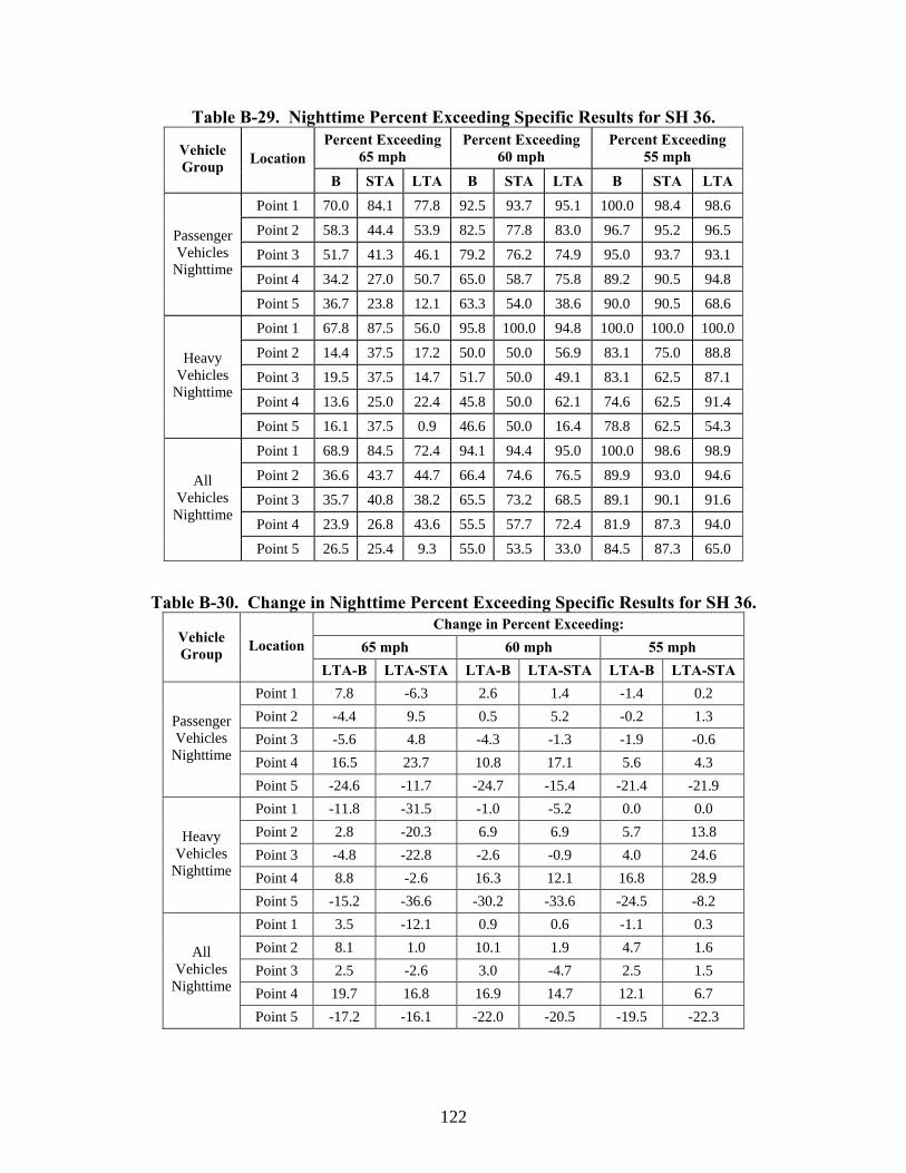
122

Table B-29. Nighttime Percent Exceeding Specific Results for SH 36. Percent Exceeding





Point 1 70.0 84.1 77.8 92.5 93.7 95.1 100.0 98.4 98.6

Point 2 58.3 44.4 53.9 82.5 77.8 83.0 96.7 95.2 96.5

Point 3 51.7 41.3 46.1 79.2 76.2 74.9 95.0 93.7 93.1

Point 4 34.2 27.0 50.7 65.0 58.7 75.8 89.2 90.5 94.8

Passenger Vehicles

Nighttime

Point 5 36.7 23.8 12.1 63.3 54.0 38.6 90.0 90.5 68.6

Point 1 67.8 87.5 56.0 95.8 100.0 94.8 100.0 100.0 100.0

Point 2 14.4 37.5 17.2 50.0 50.0 56.9 83.1 75.0 88.8

Point 3 19.5 37.5 14.7 51.7 50.0 49.1 83.1 62.5 87.1

Point 4 13.6 25.0 22.4 45.8 50.0 62.1 74.6 62.5 91.4

Heavy Vehicles

Nighttime

Point 5 16.1 37.5 0.9 46.6 50.0 16.4 78.8 62.5 54.3

Point 1 68.9 84.5 72.4 94.1 94.4 95.0 100.0 98.6 98.9

Point 2 36.6 43.7 44.7 66.4 74.6 76.5 89.9 93.0 94.6

Point 3 35.7 40.8 38.2 65.5 73.2 68.5 89.1 90.1 91.6

Point 4 23.9 26.8 43.6 55.5 57.7 72.4 81.9 87.3 94.0

All Vehicles

Nighttime

Point 5 26.5 25.4 9.3 55.0 53.5 33.0 84.5 87.3 65.0

Table B-30. Change in Nighttime Percent Exceeding Specific Results for SH 36. Change in Percent Exceeding:


LTA-B LTA-STA LTA-B LTA-STA LTA-B LTA-STA Point 1 7.8 -6.3 2.6 1.4 -1.4 0.2 Point 2 -4.4 9.5 0.5 5.2 -0.2 1.3 Point 3 -5.6 4.8 -4.3 -1.3 -1.9 -0.6 Point 4 16.5 23.7 10.8 17.1 5.6 4.3

Passenger Vehicles

Nighttime

Point 5 -24.6 -11.7 -24.7 -15.4 -21.4 -21.9 Point 1 -11.8 -31.5 -1.0 -5.2 0.0 0.0 Point 2 2.8 -20.3 6.9 6.9 5.7 13.8 Point 3 -4.8 -22.8 -2.6 -0.9 4.0 24.6 Point 4 8.8 -2.6 16.3 12.1 16.8 28.9

Heavy Vehicles

Nighttime

Point 5 -15.2 -36.6 -30.2 -33.6 -24.5 -8.2 Point 1 3.5 -12.1 0.9 0.6 -1.1 0.3 Point 2 8.1 1.0 10.1 1.9 4.7 1.6 Point 3 2.5 -2.6 3.0 -4.7 2.5 1.5 Point 4 19.7 16.8 16.9 14.7 12.1 6.7

All Vehicles

Nighttime

Point 5 -17.2 -16.1 -22.0 -20.5 -19.5 -22.3

Evaluation of Traffic Control Devices: Second Year Activities

Documents

Transcript of Evaluation of Traffic Control Devices: Second Year Activities