S.A.P.I.EN.SSurveys and Perspectives Integrating Environment andSociety 

2.2 | 2009Vol.2 / n°2 Special issueVisualizing the World

Sébastien Gadal (dir.)

Electronic versionURL: http://journals.openedition.org/sapiens/744ISSN: 1993-3819

PublisherInstitut Veolia

Electronic referenceSébastien Gadal (dir.), S.A.P.I.EN.S, 2.2 | 2009, « Vol.2 / n°2 Special issue » [Online], Online since 30 May2009, connection on 23 October 2020. URL : http://journals.openedition.org/sapiens/744

This text was automatically generated on 23 October 2020.

Licence Creative Commons

TABLE OF CONTENTS

Methods

The continuous field view of representing forest geographically: from cartographicrepresentation towards improved management planningGintautas MozgerisSébastien Gadal (ed.)

Methods for visual quality assessment of a digital terrain modelTomaz PodobnikarSébastien Gadal (ed.)

Geoarchaeology: where human, social and earth sciences meet with technologyMatthieu Ghilardi and Stéphane DesruellesSébastien Gadal (ed.)

Computer-generated Visual Summaries of Spatial Databases: Chorems or not Chorems?Robert Laurini, Monica Sebillo, Giuliana Vitiello, David Sol-Martinez and Françoise RaffortSébastien Gadal (ed.)

3D Dynamic Representation for Urban Sprawl Modelling: Example of India’s Delhi-MumbaicorridorSébastien Gadal, Stéphane Fournier and Emeric ProuteauGaëll Mainguy (ed.)

Perspectives

Integration of Geomatics in Research & DevelopmentPetter Pilesjö and Ulrik Mårtensson

Walter Christaller From “exquisite corpse” to “corpse resuscitated”Georges NicolasSebastian Gadal (ed.)

S.A.P.I.EN.S, 2.2 | 2009

1

Methods

S.A.P.I.EN.S, 2.2 | 2009

2

The continuous field view ofrepresenting forest geographically:from cartographic representationtowards improved managementplanningGintautas Mozgeris

Sébastien Gadal (ed.)

EDITOR'S NOTE

Received: 08 July 2008 — Revised: 08 January 2009 —Accepted: 23 January 2009 —

Published: 10 February 2009

Introduction

1 Enhanced visualization is usually the step towards better forest management solutions.

Maps can easily summarize and communicate results of forest inventories, and are used

as decision supporting tools. Conventional forest maps present an abstract view of

parts of the world with an emphasis on selected forest compartments, infrastructure

objects, locations of monuments, etc. They are usually addressed to numerous

identified (e.g. forest managers) and unidentified (e.g. the public) users. Aerial

photographs and later satellite images have been used for forest management for more

than a century (Hildebrandt, 1993). The invention of Geographic Information Systems

(GIS) has fundamentally changed the way visualization of geographic phenomena is

created and used, whether they are forest, coastal, urban, agricultural, etc. GIS-based

representations can portray the dynamics through animations, 3-D visualisation, and

support sophisticated spatial analyses and modelling.

S.A.P.I.EN.S, 2.2 | 2009

3

2 This paper discusses a way to describe forest geographically storing an array of

continuous surfaces of forest attributes. It is based on the combination of modern GIS

and numerical remote sensing techniques and is applicable to many other areas of

interest.

Representing forest geographically

Discrete objects or continuous fields?

3 What is “a forest”? Is it different from other phenomena represented in geographical

databases? Russian forestry scientist G.Morozov defines forest as an aggregate of trees,

which grow near-by, affect each other and the surrounding space and, therefore, are

changing their outside and inner structure (1930). This is a purely naturalistic

approach. Legally, a forest can also be defined as “at least 0.1 ha area grown-up with

trees the height of which reaches 5 m or more under natural conditions, as well as

thinned out or even having lost the vegetation naturally or because of human

activities” (Forest act of Republic of Lithuania). These examples show that definitions

directly influence the data model which will be used to describe the forest in a digital

data base.

4 There are two fundamental ways of representing geography in digital computer

environments, discrete objects and continuous fields (Longley et al., 2005). Spatial

variation in continuous fields can be itself treated as discrete or continuous (and

sometimes as a mix of the two) (e.g. Burrough, 1996; Heuvelink, 1996). Discrete models

of spatial variation are usually implemented using vector polygons while continuous

models are based on a raster approach.

Discrete Objects

5 Discrete object view assumes the world to be empty, except where it is occupied by

objects having well defined boundaries, linear or point-wise locations. Locations may

overlap and can be counted. Biological organisms or man-made objects are typical

features that fit well in this model, e.g. trees, roads, buildings, etc. Modern science and

technology would theoretically allow for a description of a forest using the model of

discrete objects. Every single tree, its location and its descriptive characteristics could

be measured and stored in a digital database. Single tree crowns may be easily

identified on aerial images or in point clouds derived using laser scanning (Figure 1.a).

However, in practice, forests have been described as “continuous fields” divided into

compartments for centuries.

S.A.P.I.EN.S, 2.2 | 2009

4

Figure 1. Two ways of representing forest in digital computer environments

Discrete objects (a) and continuous fields (b and c). (a) single tree crowns are delineated (bottom)from aerial image (top) and image, generated from laser scanned point clouds (middle) and stored in adatabase (reproduced with permission of Blom Kartta Oy). (b) volume in m3/ha represented usingdiscrete model of spatial variation; (c) stand age, height, diameter and volume per ha are representedas separate layers using continuous model of spatial variation.

Continuous fields

6 The continuous field view assumes that the real world is a series of continuous maps or

layers, each of them representing the variability of a certain attribute over the Earth’s

surface. There are no gaps in such layer: each location has one or another value of an

attribute, e.g. “forest” or “non-forest”; “young forest”, “middle aged forest” or “mature

forest”. Stand-wise forest inventories define discrete spatial objects with crisp

boundaries – forest compartments – and assign uniform characteristics within a given

polygon. Forest compartments do not overlap, the values of forest attributes are

dependant on many factors, especially human activities (Figure 1b), and change

abruptly on the boundary of a compartment. The main concepts of forest compartment

and stand-wise forest inventories were developed centuries ago, long before the

introduction of mathematical statistics, computers and remote sensing. This historical

way of representing spatial variation with discrete model is thus widely used in

operational forest inventories and management planning.

7 However, the description of forest attributes as continuous surfaces is getting more

popular today. All attributes vary continuously and smoothly over space and their

values are available at any location or point and stored in digital databases (Fig. 1c). In

this paper we focus on the method that describes forest attributes as continuous

surfaces, an approach that can be applied to any other natural phenomena which

present smooth variation in space.

S.A.P.I.EN.S, 2.2 | 2009

5

How to get continuous surfaces of forest attributes?

8 For each given attribute, a unique value should be recorded at every location or point

inside the forest (and this value will be equal to zero outside). Many countries have

been using this approach for decades to get information for strategic forestry planning

from their National forest inventories (by combining sampling methods with remotely

sensed data).(e.g. Tomppo, 1993; Nilsson, 1997; Tomppo et al., 1999; Gjersten et al., 2000,

Franco-Lopez et al., 2001 and many other authors). It is used to aggregate detailed

stand-wise forest information to be represented at a coarser scale (e.g. Kurlavicius et al.,

2004) or when more detailed information is not available (Paivinen et al., 2001).

9 Forest information is organized using a grid of systematically distributed virtual

samples or points corresponding to pixels in a raster data model. Such points may be

distributed rather sparsely1 or may form very dense networks (e.g. 25x25 m, 1x1 m and

so on). Each point represents an array of several forest attributes of interest at that

location. Pixels of rasters and images may also be considered as virtual points and

digital numbers of e.g. satellite images replaced by estimated forest characteristics.

Such point-wise or pixel-wise information may be used for forest inventories that

support tactical and operational forest management planning.

10 A surface of forest characteristic or virtual samples of forest characteristics can be

obtained by:

measuring all of them in the field (Gunnarsson et al., 1999), however this is rather expensive

since a separate measurement is required for each point. In the case of Landsat TM for

instance, someone would have to estimate forest stand volume or age for a 30x30m grid

systematically.

measuring a subset in the field and extrapolate the results for the other locations using

geostatistical methods (such as the kriging interpolation, Gunnarsson et al., 1999). In this

case spatial autocorrelation should be present in the studied phenomenon and with large

sample volume, we may be back to the previous case.

measuring them on images using stereo photogrammetric equipment, however this is labour

consuming and expensive too

modelling the surfaces of forest attributes using available auxiliary information (usually in

digital format) that correlates with forest characteristics – satellite and aerial images,

historical forest inventory information, GIS databases, etc. This approach is the cheapest,

and is detailed below.

11 In the case of raster surfaces, layers of auxiliary information (e.g. satellite images,

digital elevation models, soil type maps, etc.) are available for the whole area of

interest. Forest attributes are measured in the field for a limited number of locations;

they may even be already available from other types of inventories2. Next, all pixels are

divided into two groups: A-observations and B-observations. Both input (auxiliary) and

output (forest attributes) data are known for the B-observations but only input

(auxiliary) data are known for the A-observations. The task is to get the forest

characteristics on the basis of auxiliary information for all A-observations utilizing the

knowledge on relationships between auxiliary and field information, developed using

B-observations. Numerous parametric and nonparametric methods of estimations have

been used for that purpose3 and they give similar estimation accuracies (Mozgeris,

2000). However the k-nearest neighbor estimation is favored in most forest inventory

•

•

•

•

S.A.P.I.EN.S, 2.2 | 2009

6

oriented applications and it is expected to be of great potential to model other

geographic phenomena: It is well documented in the literature, easy to understand and

implement (free software available), and it can accommodate a wide range of auxiliary

information.

12 The k-nearest neighbor method (Tomppo, 1993) or multi-dimensional version of

inverse distance weighted technique familiar to the majority of GIS users, can be briefly

described as follows: Euclidean distance di,pis calculated between each A-observation

sampling unit p in n dimensional feature space of auxiliary information and B-

observation unit i with field measured forest characteristics. n here refers to the total

number of layers of auxiliary information – channels of satellite image, parameters

from stand-wise inventories, etc. k (1-10 and more) distances di,p - d(1),p ... d(k),p, (d(1),pF0A3 ...F0A3

d(k),p ) are found and the weight is calculated:

(1)

13 Value of forest parameter M on sample unit p of A-observation equals:

(2)

14 Where m(j),p, j=1,...k – values of forest parameter M in k nearest B-observation plots to p

in n dimentional space.

15 The influence of different settings on the accuracy of estimations has been widely

studied: for instance, the Mahalanobis distance has been used instead of the Euclidean

one without significant success indeed (Mozgeris, 1996; Franco-Lopez et al., 2001). The

number of k minimal amount of B-observations has been discussed in-depth a decade

ago (Tomppo, 1996; Tokola et al., 1996; Mozgeris, 1996; Nilsson, 1997) to develop general

methodological framework for the use of k-nearest neighbor estimation in remote

sensing assisted forest inventories.

16 Digital satellite images have been the major source of auxiliary information to get

continuous surfaces of forest characteristics. Principal component transformations and

pre-stratification are used to facilitate the integration of satellite images with other

types of auxiliary information4. Geographical distance between A-observations and B-

observations is also taken into account (Katila et al., 2001). An expert system (Wang,

2006), different techniques to weight alternative estimates (Mozgeris, 2000), and,

finally, optimization techniques called genetic algorithm (Tomppo et al., 2004; Tomppo

et al., 2006), have been used to improve the accuracies of point-wise estimates taking

into account diverse sources of auxiliary information and parameters of estimators.

However, despite the intensive research on the optimization of estimation techniques,

it is generally concluded that no universal solution can satisfy the needs of all users.

Several approaches should be tested using modern computation tools to find the best

one, fitting certain conditions.

S.A.P.I.EN.S, 2.2 | 2009

7

The use of continuous surfaces of forestcharacteristics

17 Natural phenomena usually exhibit both continuous and discrete behaviour (Burrough,

1996). Such spatial continuity (even when disrupted by abrupt changes) is rather

difficult to visualize using discrete model or choropleth presentations. Any natural

characteristic sampled and measured in the field can be represented for a certain

location using the model of point-wise characteristics. The array of such characteristics

depends on the objectives of the representation (improved visual representation, input

for GIS based modelling, enhanced opportunities for natural resource inventory and

management planning, etc.).

18 The operational forest management planning approaches in many countries require

some discretisation of continuous surfaces into areal units, corresponding to forest

compartments. The A-observations (points, pixels, etc.) are easily grouped based on the

values of certain characteristics (e.g. all set of characteristics that are used to single-out

forest compartments) to form discrete units (conventional compartments, polygons

where certain assortment is available for logging, etc.). Since such units can change in

size, shape and role, they are called virtual or dynamic compartments. The concept of

dynamic forestry unit, developed following the principles described above, has been

discussed previously (Holmgren and Thuresson, 1997; Gunnarsson et al., 1999), but it

has not yet received much attention in the forest inventory literature.

19 Here we present two possible uses of the estimated surfaces of forest characteristics to

solve conventional stand-wise forest inventory tasks, which may be successfully

adopted for other applications. The first one allows improved automatic delineation of

discrete units, corresponding to forest compartments. The other facilitates change

detection by combining single acquisition time satellite images and information from

stand-wise inventories (which may be adopted to detect the changes in other spatially

distributed resources too).

Improved automatic stand delineation

20 Forest compartments are usually singled-out in stand-wise inventories using methods

of visual interpretation of high resolution aerial or satellite images5. Automatic stand

delineation has always been a very challenging task both for researchers and for forest

inventory practitioners. Traditional image classification algorithms, which are

successful for many other applications, (such as maximum likelihood, parallelepiped or

minimum distance), usually do not work for forest management planning. This is

mainly due to the fact that foresters need to have stand-wise information on numerous

stand parameters rather than discrete pixel by pixel classes and large approximations

are needed to express continuous forest characteristics with few discrete classes. How

to use segmentation to divide the image into spatially contiguous regions that are

homogeneous regarding to their radiometric characteristics has been abundantly

documented in the last two decades (Tomppo, 1987, 1988; Hagner, 1990; Hame, 1991;

Parmes, 1993; Olsson, 1994; Haapanen & Pekkarinen, 2000). Similar research has been

carried out in Lithuania a decade ago as well, even though the results have not been

used operationally (Mozgeris et al., 2000; Mozgeris, 2001). However, new approach in

segmentation tactics – estimation of forest characteristics for every pixel of satellite or

S.A.P.I.EN.S, 2.2 | 2009

8

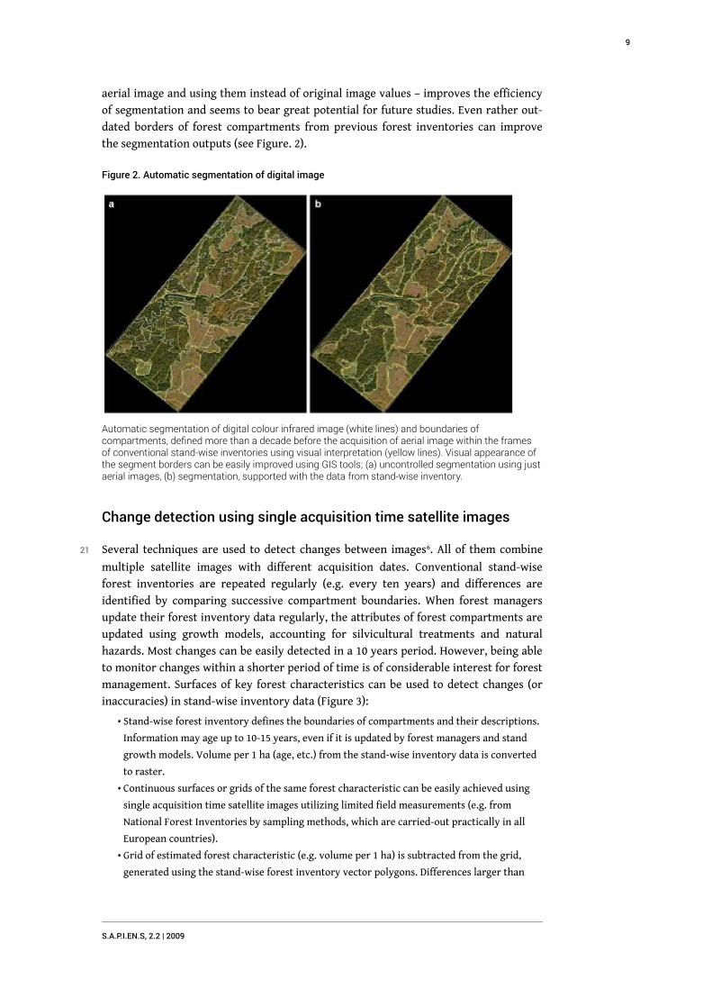
aerial image and using them instead of original image values – improves the efficiency

of segmentation and seems to bear great potential for future studies. Even rather out-

dated borders of forest compartments from previous forest inventories can improve

the segmentation outputs (see Figure. 2).

Figure 2. Automatic segmentation of digital image

Automatic segmentation of digital colour infrared image (white lines) and boundaries ofcompartments, defined more than a decade before the acquisition of aerial image within the framesof conventional stand-wise inventories using visual interpretation (yellow lines). Visual appearance ofthe segment borders can be easily improved using GIS tools; (a) uncontrolled segmentation using justaerial images, (b) segmentation, supported with the data from stand-wise inventory.

Change detection using single acquisition time satellite images

21 Several techniques are used to detect changes between images6. All of them combine

multiple satellite images with different acquisition dates. Conventional stand-wise

forest inventories are repeated regularly (e.g. every ten years) and differences are

identified by comparing successive compartment boundaries. When forest managers

update their forest inventory data regularly, the attributes of forest compartments are

updated using growth models, accounting for silvicultural treatments and natural

hazards. Most changes can be easily detected in a 10 years period. However, being able

to monitor changes within a shorter period of time is of considerable interest for forest

management. Surfaces of key forest characteristics can be used to detect changes (or

inaccuracies) in stand-wise inventory data (Figure 3):

Stand-wise forest inventory defines the boundaries of compartments and their descriptions.

Information may age up to 10-15 years, even if it is updated by forest managers and stand

growth models. Volume per 1 ha (age, etc.) from the stand-wise inventory data is converted

to raster.

Continuous surfaces or grids of the same forest characteristic can be easily achieved using

single acquisition time satellite images utilizing limited field measurements (e.g. from

National Forest Inventories by sampling methods, which are carried-out practically in all

European countries).

Grid of estimated forest characteristic (e.g. volume per 1 ha) is subtracted from the grid,

generated using the stand-wise forest inventory vector polygons. Differences larger than

•

•

•

S.A.P.I.EN.S, 2.2 | 2009

9

some marginal value indicate forest changes and, up to some extent, inaccuracies of stand-

wise inventory.

Figure 3. Forest change detection

Forest change detection subtracting grids of volume in m3/ha represented using discrete model ofspatial variation (a) and continuous model of spatial variation (b). (a) forest inventory data from 1988;(b) derived surface using SPOT 4 HRVIR satellite image, ~600 field plots data from 1999 and k-nearestneighbor estimation. (c) SPOT HRVIR image and boundaries of compartments defined by stand-wiseinventory 3 years after the satellite image acquisition (green lines) together with the identifiedchanges: clear-cuts (yellow striped pattern, detected), non-clear felling (blue striped pattern), clear-cutafter satellite image acquisition (green striped pattern, not detected).

22 This gives a brief and general description of the idea. To have practical value for

operational forest management, other aspects need to be taken into account, such as

the rules to classify the differences according to the types of change, the principles of

ground-truthing7, accuracy issues of stand-wise information, etc.

Opportunities for other fields

23 This paper focuses on the opportunities to use geomatics for forest inventory. The

approaches discussed here are well known to forest inventory professionals and could

be of great interest for other disciplines. As mentioned above, most natural phenomena

usually exhibit both continuous and discrete behaviour (Burrough, 1996), and natural

characteristic that can sampled and measured in the field can be represented using the

model of point-wise characteristics. Different outputs can be generated using different

array of auxiliary information, based on similar processing mechanisms. We use here

the non-parametric k-nearest neighbour estimator to get the dependant variable from

various independent variables – the non-parametric methods are recommended as an

alternative to the traditional approaches based on regression models. The main

S.A.P.I.EN.S, 2.2 | 2009

10

advantage of non-parametric methods is that they retain the full range of variation of

the data as well as the covariance structure of the population (Moeur and Stage, 1995).

And finally, they are more easy to use and accessible to everyone, even to the amateur

in statistics.

24 Single acquisition time satellite images, transformed into continuous surfaces of major

forest characteristics, have been successively used together with the data from stand-

wise forest inventories to detect clear-cut areas in the forest. The comparison of

several independently produced classified images is of course the most obvious method

to detect changes in the state of a geographic phenomenon (Singh, 1998). But when

images are not available at a given time, they can be inferred from a model of

evolution.

25 In conclusion, powerful tools for image segmentation are available nowadays. In

particular, the fuzzy logic based software by Definiens emulates the human cognitive

processes to perform automated image analysis8. The technology is context-based and

identifies objects rather than simply examining individual pixels. This approach can be

used to monitor a vast range of natural and social phenomena such as natural resource

management or infrastructure planning.

BIBLIOGRAPHY

Burrough P.A. (1996). Natural objects with indeterminate boundaries. In: Geographic Objects with

Indeterminate Boundaries, Burrough, P.A. and Frank, A.U. (eds.), Taylor & Francis, pp. 3-28

Eastman J.R. & J.E. Mckendry (1991). Explorations in Geographic Information Systems

Technology. Volume 1. Change and Time Series Analysis, UNITAR European Office, Geneva, 86.

Franco-Lopez H., A. Ek & M.E. Bauer (2001). Estimation and Mapping of Forest Stand Density,

Volume, and Cover Type Using the k-Nearest Neighbors Method, Remote Sensing of

Environment, Vol.77, pp.251– 274.

Gjertsen A. K., S. Tomter & E. Tomppo (2000). Combined Use of NFI Sample Plots and Landsat TM

Data to Provide Forest Information on Municipality Level. In: T. Zawil-Niedzwinski, & M. Brach

(Eds.). Remote sensing and forest monitoring: Proceedings of IUFRO conference, 1 – 3 Jun. 1999,

Rogow, Poland. Luxembourg: Office for Official Publications of the European Communities, pp.

167– 174.

Gunnarsson F. et al. (1999). On the potential of kriging for forest management planning,

Scandinavian journal of forest research, Vol. 13, pp.237 – 245.

Haapanen R. & A.Pekkarinen (2000). Utilising satellite imagery and digital detection of clear

cuttings for timber supply management / Manuscript of paper submitted to ISPRS, Vol. XXXIII,

Amsterdam. 8..

Hagner O. (1990). Computer Aided Forest Stand Delineation and Inventory Based on Satellite

Remote Sensing. In: The usability of remote sensing for forest inventory and planning: proc. from

SNS/IUFRO workshop, Umea, 26-28 February. Umea, pp.94-105.

S.A.P.I.EN.S, 2.2 | 2009

11

Hame T. (1991). Spectral interpretation of changes in forest using satellite scanner images //

Acta Forestalia Fennica. Vol. 222. 112 p.

Heuvelink G.B.M. (1996). Identification of Field Attribute Error under Different Models of Spatial

Variation, International Journal of Geographic Information Systems, Vol.10, No.8, pp. 921-935.

Hildebrandt G. (1993). Central European contribution to remote sensing and photogammetry in

forestry, In: Forest resource inventory and monitoring and remote sensing technology:

Proceedings of the IUFRO centennial meeting in Berlin, Japan Society for Forest Planning Press,

Tokyo, Japan, pp. 196-212.

Holmgren P. & T.Thuresson (1997). Applying objectively estimated and spatially continuous

forest parameters in tactical planning to obtain dynamic treatment units, Forest Science, Vol. 43,

pp.317 – 326.

Kasperavičius A., A. Kuliešis & Mozgeris G. (2000). Satellite imagery based forest resource

information and its application for designing the National forest inventory in Lithuania, In: T.

Zawil-Niedzwinski, & M. Brach (Eds.). Remote sensing and forest monitoring: Proceedings of

IUFRO conference, 1 – 3 Jun. 1999, Rogow, Poland. Luxembourg: Office for Official Publications of

the European Communities, pp.50-58.

Kuliesis A. & A. Kasperavicius (1999). National Forest Inventory Guide, Kaunas, 133 p. (in

Lithuanian)

Kurlavicius, P. et al. (2004). Identifying high conservation value forests in the Baltic States from

forest databases, Ecological Bulletins 51, pp.351-366.

Lilesand T.M. & R.W. Kiefer (1994). Remote sensing and image interpretation, John Wiley & Sons

Inc., 750 p.

Longley P.A. et al. (2005). Geographic Information Systems and Science, 2nd Edition, John Wiley &

Sons, Inc., 517 p.

Moeur M. & A.R. Stage (1995). Most Similar Neighbor: an Improved Sampling Inference Procedure

for Natural Resource Planning, Forest Science 41 (2), 337–359.

Morozov G.F. (1931). Study on the forest, Moskva-Leningrad, Goslesbumizdat, 440 p. (in Russian).

Mozgeris G. (1996).Dynamic Stratification for Estimating Pointwise Forest Charakteristics. Silva

Fennica, Vol. 30(1), 61-72.

Mozgeris G. & A. Augustaitis (1999). Using GIS techniques to obtain a continouos surface of tree

crown defoliation, Baltic forestry, Vol. 5, No.1, pp.69-74.

Mozgeris G., A.Kuliešis & A.A. Kuliešis (2000). Looking for new solutions in delineating forest

stands: segmentation of multi-source data, In: Proc. of III International Symposium "Application

of Remote Sensing in Forestry", Faculty of Forestry, Technical University in Zvolen, Zvolen,

September 12-14, 2000, ISBN 80-968494-0-9, p. 123-132

Mozgeris G. (2000). Estimation of point-wise forest characteristics using two-phase sampling,

Vagos, Transactions of Lithuanian University of Agriculture. Vol. 48(1), 28-38 (In Lithuanian).

Mozgeris G. (2001). Research on application of satellite image segmentation for stand-wise forest

inventory. Vagos, Transactions of Lithuanian University of Agriculture 52 (5), 15-23 (In

Lithuanian).

Nilsso M. (1997). Estimation of Forest Variables Using Satellite Image Data and Airborne Lidar.

PhD thesis, Swedish University of Agricultural Sciences, The Department of Forest Resource

Management and Geomatics. Acta Universitatis Agriculturae Sueciae. Silvestrias, 17.

S.A.P.I.EN.S, 2.2 | 2009

12

Olsson H. (1994). Monitoring of local reflectance changes in boreal forests using satellite data /

Report 7, Dept. of biometry and forest management, Swedish university of agricultural sciences.

Umea.

Paivinen R. et al. (2001). Combining Earth Observation Data and Forest Statistics, EFI Research

Reports 14, European Forest Research Institute and Joint Research Centre – European

Commission, 101.

Parmes E. (1993). Segmentation of Landsat and Spot satellite imagery, Photogrammetric Journal

of Finland. Vol. 13. 52-58.

Poso S., R. Paananen & M. Simila (1987). Forest inventory by compartments using satellite

imagery, Silva Fennica, Vol. 21 (1), 69-94.

Singh A. (1989). Digital change detection techniques using remotely-sensed data. Review Article,

International Journal of Remote Sensing, Vol. 10, No. 6, 989-1003.

Tokola T. et al. (1996). Point Accuracy of a Non-parametric Method in Estimation of Forest

Characteristics with Different Satellite Materials. International journal of remote sensing, Vol.

17, No. 12, 2333-2351.

Tomppo E., C. Goulding, C. & M. Katila (1999). Adapting Finnish multisource forest inventory

techniques to the New Zealand preharvest inventory, Scandinavian Journal of Forest Research,

Vol.14, 182– 192.

Tomppo E. (1996). Multi-source National Forest Inventory of Finland, In: R.Vanclay, J. Vanclay, &

S. Miina (Eds.), New thrusts in forest inventory: Proceedings of the subject group 4.02-00 'Forest

Resource Inventory and Monitoring' and subject group 4.12-00 'Remote Sensing Technology', vol.

1, IUFRO XX World Congress, 6 - 12 Aug. 1995 Tampere, Finland, European Forest Institute,

Joensuu, Finland, 27- 41.

Tomppo E. (1993). Multi-source national forest inventory of Finland, Proc. Of Ilvessalo

symposium on national forest inventories. IUFRO S4.02, Finnish forest research institute,

University of Helsinki. Helsinki, 52-60.

Tomppo E. (1987). Stand delineation and estimation of stand variates by means of satellite

images, Remote sensing-aided forest inventory: proc. from seminars organized by SNS and

Takssttoriklubi, Hyytiala, Finland, December 10-12, 1986: research notes No. 19. University of

Helsinki. Dept. of forest mensuration and management. Helsinki, 60-76.

Tomppo E.(1988). Standwise forest variate estimation by means of satellite images, Satellite

imageries for forest inventory and monitoring: experiences, methods, perspectives: proc. from

the IUFRO Subject Group 4.02.05 meeting in Finland, Aug. 29 – Sept. 2, 1988: research notes No.

21. University of Helsinki, Dept. of forest mensuration and management. Helsinki, 103-111.

Wang G (1996). An expert system for forest resource inventory and monitoring in the frame of

multi-source data, University of Helsinki. Department of forest resource management.

Publications 10. Helsinki, 173.

NOTES

1. e.g. 250x250 m, as in the case of forest area in Lithuanian National forest inventory by

sampling methods (Kasperavičius et al., 1999)

2. For instance almost all European countries carry-out National forest inventories, which

include systematic measurements in the forest following some statistical schemes

S.A.P.I.EN.S, 2.2 | 2009

13

3. regression (e.g. Hagner, 1990; Nilsson, 1997; Mozgeris and Augustaitis, 1999), static and

dynamic stratification (e.g. Poso et al., 1987; Mozgeris, 1996), k-nearest neighbor estimation (e.g.

Tomppo, 1993; Gjersten et al., 2000; Tokola et al., 1996), most similar neighbour estimation (Moeur

and Stage, 1995), GIS-driven pseudo-raster transformations (Kurlavicius et al., 2004), etc.

4. such as historical forest inventory information, which may be outdated and rather inaccurate

for direct use but can still correlate with the actual forest characteristics, general use GIS data,

soil maps, digital elevation models and their derivatives, etc. (e.g. Tokola et al., 1997; Katila et al.,

2001; Mozgeris, 2006).

5. such as Ikonos, QuickBird, sometimes SPOT, Landsat or similar, depending on the targeted

level of details.

6. image differencing, image regression, image ratio, principal components analysis, comparison

of independent classification results, classification of integrated information from different dates

of acquisition (Singh, 1998; Eastman and McKendry, 1991).

7. Ground truthing is the act of physically going to a field to determine the cause of variability

detected in an image.

8. www.definiens.com

ABSTRACTS

Enhanced vizualization leads to better forest management solutions. This paper discusses the

application of numerical remote sensing and geographic information systems to forest inventory.

Natural phenomena usually exhibit both continuous and discrete behaviour. Discrete models

have been used since the inception of aerial photography, long before the introduction of

mathematical statistics, computers or remote sensing but today, forest attributes can also be

described as continuous surfaces. This paper briefly presents the uses and limitations of a

popular non-parametric estimator (the k-nearest neighbour): it improves visual representation,

and provides a better input for GIS based modelling, thus facilitating natural resource inventory

and management planning. However, in many countries, the operational forest management

planning approaches still require some discretisation of continuous surfaces into areal units,

corresponding to virtual –or dynamic- forest compartments.

INDEX

Subjects: Methods

AUTHORS

GINTAUTAS MOZGERIS

GIS Education and Research Centre, Institute of Environment, Lithuanian University of

Agriculture, Studentu 11, LT-53361, Akademija, Kaunas r., Lithuania

S.A.P.I.EN.S, 2.2 | 2009

14

Methods for visual qualityassessment of a digital terrainmodelTomaz Podobnikar

Sébastien Gadal (ed.)

EDITOR'S NOTE

Reviewed by two anonymous referees.

Received: 8 June 2008 – Revised: 16 January 2009 – Accepted: 26 January 2009 –

Published: 29 January 2009.

Introduction

1 A digital terrain models (DTMs) is a continuous surface that, besides the values of

height as a grid (known as a digital elevation model—DEM), also consists of other

elements that describe the topographic surface, such as slope or skeleton (Podobnikar,

2005). Different techniques for the generation of DTMs have been developed since their

inception more than fifty years ago (Miller and Laflamme, 1958; Doyle, 1978). The first

decades focused mainly on models’ reliability. The common techniques for quality

assessment were based on the statistical comparison of small reference areas of higher

quality with the created DTM in order to find outliers. Until the end of the 90s, high

quality terrain data were acquired mainly photogrammetrically using aerial

photographs and manual stereo measurements or matching techniques, or by

vectorisation of contour lines from topographical maps and attribution.

2 The quality of DTMs significantly increased over the last decade due to three significant

factors:

The first was the introduction and development of new methods for data acquisition,

especially from satellites and airplanes. At small scales (coarser spatial resolution)

S.A.P.I.EN.S, 2.2 | 2009

15

radar interferometric techniques (IfSAR) had been applied to generate global DTMs1

(Burrough and McDonnell, 1998; Maune, 2001). For larger scales and more local usage,

airborne laser scanning (ALS) techniques have been applied2 (e.g. Kraus and Pfeifer,

1998).

The second factor is the increasing availability of additional data sources that are

useful for the DTM quality assessment or enhancement. In addition to the aerial

photographs and contour lines, different point datasets with height attributes could

also be applied, such as fundamental geodetic network points, boundary points of land-

cadastre, databases of buildings, spot elevations, and other related datasets such as

highway construction or hydrological network measurements. Even datasets without

height attributes such as lines of a hydrological network, roads, railways, and standing

water polygons can be used (Podobnikar, 2005). These additional data sources can

provide valuable input for integrated DTM production, as exemplified in Slovenia

(Podobnikar, 2005) and in Europe (EuroGeographics, 2008).

Thirdly, applications using DTMs are now part of our everyday lives (e.g., Google Earth3,

Microsoft Virtual Earth4, NASA World Wind5, Radrouten Planer6…). This trend can also

have some impact on the quality of the DTMs used if it influences usability

significantly.

3 The higher the resolution, the more difficult the evaluation of input data quality and

the assessment of the resulting DTM are. Experience indicates that the effort is

proportional to the square of the inverse value of horizontal resolution. High

resolution DTMs are thus more prone to errors. Visual methods can be very important

for the evaluation of spatial data and can balance some weaknesses of statistical

methods. They are still underused for at least three reasons. Visual approaches being

qualitative are generally more neglected than statistical ones which are considered to

be more objective. The other reasons for the lower acceptance of visual methods lie in

the insufficient graphical capabilities of computers until recently and in the longer

tradition of using statistical methods. Finally, visualisation of spatial data has

traditionally been part of cartography. The main emphasis of this paper is to focus

attention on visual methods as a powerful tool for quality assessment.

Towards data quality assessment

4 The quality of spatial analysis depends on data quality, (data) model relevance and on

the way they interact (Burrough and McDonnell, 1998). The model (or nominal ground)

is a conceptualisation and representation (abstraction) of the real world, i.e., a selected

representation of space, time, or attributes (Aalders, 1996). The datasets—in our case

the DTMs—are realised by the type of spatial object to which variables refer on the

level of measurement of these variables. The model relevance is a semantic quality of

the representation by which a complex reality is captured. Data quality refers to the

performance of the dataset given the specification of the data model (Haining, 2003).

Model quality—a DTM definition

5 The DTM dataset is an approximation of the reality, based on a nominal ground. A

semantically reliable and high quality data model (as a base for the DTM generation)

should be carefully defined. The DTMs might vary depending on their purpose, the

S.A.P.I.EN.S, 2.2 | 2009

16

quality of data sources or interpolation algorithms, the experience of the operators,

etc.

6 A basic distinction can be made between digital elevation models (DEMs) and digital

terrain models (DTMs) (Burrough and McDonnell, 1998; Podobnikar, 2005; Sutter et al.,

2007)7. The DEM is one of the most used ‘raster datasets’ (a grid or a matrix) in

geographical information systems (GIS). An elevation value (height) is attributed to

each square cell of the grid. The set of cell heights can then be interpreted in two ways:

In the first approach, each cell represents a discrete area, hence the entire cell area is

assumed to have the same value, the changes occur only at the edges of the cells. In the

second approach, the area between the cell centres is assumed to have some

intermediate values. This approach is closer to the DTM definition. The DTM is

considered as a continuous, usually smooth surface which, in addition to height values

(as DEMs), also contains other elements that describe a topographic surface: slope,

aspect, curvature, gradient, skeleton (pits, thalwegs, saddles, ridges, peaks), and others.

In this study, we focus on DTM but the methods and results are largely applicable to

DEM also.

Data quality

7 Quality assessment methods can be distinguished a priori or a posteriori. Before

generating the DTM, one can know the expected quality that result from our capacity

and what quality is required with regard to the respected standards. These two factors

enable regular production and usability of the DTM. The a priori assessments are based

mostly on analyses of the datasets and methods for the DTM production while the a

posteriori methods are based on the final DTM as described in this paper.

8 One of the DTM quality assessment goals is to fulfil the requirements of spatial data

standards. The ISO (International Organization for Standardization) distinguishes five

elements of data quality: completeness; logical consistency; and three types of accuracy

(positional, temporal, and thematic). This paper is concerned with accuracy, defined as

a difference between the value of a variable, as it appears in a dataset, and the value of

the variable in the data model (or “reality”). More specifically, we are referring to

positional accuracy. We can distinguish between absolute and relative accuracy in terms

of nature of the data. The position (horizontal or vertical) of the objects (e.g. ridges or

sink holes as part of the DTM) could be assigned to absolute accuracy and the

irregularity of the shapes of objects to the relative accuracy, that is, morphologically

relative to a general position. The term precision is considered as a component of

accuracy, related to the scale, resolution, and also to the generalisation of datasets

(Podobnikar, 2008).

9 The term error is used for lack of quality, or little or no accuracy. In addition to

mistakes—in its widest meaning—it also refers to the statistical concept of variation

(Burrough and McDonnell, 1998). The variation corresponds to random errors, thus

incorrect spatial variation can be considered as systematic or gross error. According to

these definitions, a level of accuracy (or error) can be described with a root mean

square error (RMSE) and precision with a standard deviation or a standard error (σ).

S.A.P.I.EN.S, 2.2 | 2009

17

Basic standards for the DTM quality assessment

10 Most data quality standards for the DTMs encompass several quality requirements, but

methods for quality control are seldom used. Visual quality control methods are even

less often included. A certain level of standardisation is provided by USGS (1998).

National Geospatial-Intelligence Agency (NGA)8 developed a “Digital Terrain Elevation

Data” (DTED) standard for uniform matrix DTMs. It provides basic quantitative data for

applications that require terrain elevation, slope, and/or surface roughness

information9. The metadata of quality are roughly described with absolute horizontal

(circular)/vertical (linear) error.

11 EuroGeographics10 is currently developing a pan-European grid called EuroDEM11. Since

the DTM is produced from various national DTMs, an important part of the project

consists in the standardisation/harmonisation of the various coordinate systems,

resolutions, and accuracies.

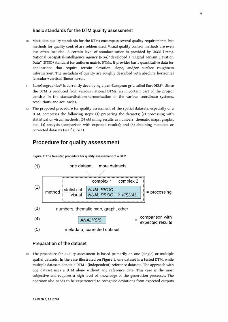
12 The proposed procedure for quality assessment of the spatial datasets, especially of a

DTM, comprises the following steps: (1) preparing the datasets; (2) processing with

statistical or visual methods; (3) obtaining results as numbers, thematic maps, graphs,

etc.; (4) analysis (comparison with expected results); and (5) obtaining metadata or

corrected datasets (see figure 1).

Procedure for quality assessment

Figure 1: The five-step procedure for quality assessment of a DTM

Preparation of the dataset

13 The procedure for quality assessment is based primarily on one (single) or multiple

spatial datasets. In the case illustrated on Figure 1, one dataset is a tested DTM, while

multiple datasets denote a DTM + (independent) reference datasets. The approach with

one dataset uses a DTM alone without any reference data. This case is the most

subjective and requires a high level of knowledge of the generation processes. The

operator also needs to be experienced to recognise deviations from expected outputs

S.A.P.I.EN.S, 2.2 | 2009

18

and to predict the most useful kind of analysis. The approach with multiple datasets

uses a DTM and additional reference datasets. The reference datasets can be the DTMs

as regionally continuous data, lines, or points. The basic criterion for selecting the

appropriate reference data is that the quality should be at least as high as expected

from the tested DTM. The reference data should be representative (of sufficient

quantity), therefore distributed with a certain degree of regularity and significance

with respect to the whole area. These methods are not convenient for areas where

availability of the reference datasets is very low (e.g. currently, Mars datasets).

Processing with statistical and visual methods

14 Processing with both statistical and visual methods is the primary focus of this

research. The methods addressed differ according to whether they use one or multiple

datasets and by their expected outputs. The single dataset method may allow more

techniques for processing. These techniques may be used one after another. We

classified them into two complexes: techniques using numerical processing and those

using visualisation (Figure 1). Those in the first complex apply statistical and visual

methods, while those in the second complex additionally apply visual methods only.

With respect to visual methods, multiple techniques from complex 1 may be followed

with single techniques of complex 2, and vice versa. Furthermore, some techniques of

complex 1 can generate input for statistical methods but not for visual ones, some of

them are useful just for visual methods, and the others for both statistical and visual

methods. Statistical methods are denoted by /S/ and the visual by /V/. We propose the

following classification of the methods:

Statistical assessment

on one spatial dataset /S1/

on multiple datasets /Sn/

Visual assessment (classification is partly referring to Berry’s (1987) classification of spatial

analysis)

visualisations according to spatial analytical operations /V1

on one dataset /V11

on multiple datasets /V1n/

Visualisations according to spatial statistical analysis /V2/ (/V21/, /V2n/)

Non-spatial visualisations /V3/ (/V31/, /V3n/)

Other visualisation techniques/other algorithms /V4/ (/V41/, /V4n/)

Results of the processing

15 The results of the processing include numbers for the statistical assessment methods,

and thematic maps, various non-spatial visualisations, and other approaches to

visualisations for the visual assessment methods.

Analysis of the results

16 The next step is the comparison of the results with what can be expected from the

quality of the data model. This is done via statistical methods (e.g. calculated RMSE

with allowed RMSE). The analysis of results of the visual methods is more complex and

less objective. In this case the results are compared with the “thresholds” and already

•

◦

◦

•

◦

▪

▪

◦

◦

◦

S.A.P.I.EN.S, 2.2 | 2009

19

“established” models. The visual methods require experience obtained through

training. Fortunately some visual methods are generated fairly effortlessly and are

easily understandable by a wide audience (as in Figure 2).

Final evaluation

17 As a final result, the datasets (DTMs) are evaluated by statistical or visual methods

within the reports. Parameters of quality control are assessed and presented as

extended standard metadata. An additional advantage is the opportunity for correction

of the datasets—DTMs (Podobnikar, 2005).

Statistical methods for data quality assessment

18 The statistical methods for quality control are also known as geometrical (when a

topographic description of particular DTM objects is applied), stochastic (non-

deterministic), or even mathematical (using mathematical methods). The most

common approaches are analytical and empirical. The analytical approaches are

primarily used when reference data is not available (Martinoni and Bernhard, 1998).

Methods based on one dataset /S1/

19 The following parameters for quality assessment can be considered (descriptive

statistic): arithmetical mean of heights, slopes, etc.; standard deviation σ; covariant

function for heights, slopes, and volumes (Östman, 1987), rang (minimum/maximum),

and Koppe’s formula adapted with other coefficients (Ackermann, 1978; Kraus, 1994);

and autocorrelation analysis (Lee and Marion, 1994). The local methods entail

description with variograms and correlograms (Wood, 1996; López, 2000) and

measurement of the fractal dimensions of terrain (Wood, 1996) and terrain curvature.

20 To analyse the estimated uncertainty of height data, Monte Carlo methods can be

applied (Goodchild, 1995; Fisher, 1996; Podobnikar, 2005). The robust estimation

method is based on statistical elimination of data that are not well enough

autocorrelated to a certain threshold (Kraus and Pfeifer, 1998). Additionally, error

assessment for the surroundings of a selected point on a surface may employ the

“perfect inspector” hypothesis (López, 2000). A complex analytical method of spectral

terrain analysis has been developed by Tempfli (1980; 1999), Frederiksen and Jacobi

(1980), Russel et al. (1995), and Russel and Ochis (1995). The sensitivity analysis method

was developed by Martinoni and Bernhard (1998). Accuracy can be also estimated by

considering the density of the original datasets and local terrain curvature (Kraus et al.,

2004).

21 Another series of assessments includes various topological controls using vector

contour lines developed to correct data in the following manners: nodes between two

lines should have identical attributes; crossed lines should be eliminated; different

heights of points and lines with identical coordinates should be unified; and contours

with only one point (node) should be eliminated (Podobnikar, 2005; Figure 6). Other

methods can be used to eliminate gross errors such as determination of the slopes that

are too steeply inclined, and methods for determination of the height differences on

the basis of control of neighbour contours (Larson, 1996).

S.A.P.I.EN.S, 2.2 | 2009

20

Methods based on multiple datasets /Sn/

22 Possible methods using a DTM and additional reference DTM(s) include: computing a

mean error (M) (indicator for a systematic error), root mean square error (RMSE)

(indicator for a random error after the systematic component has been eliminated),

range (minimum/maximum), and others. Furthermore, the following tests are

proposed: statistical covariance, regression, histograms, volume differences, and

others.

23 The methods for comparison of the DTM with reference lines and points are similar to

the methods described using continuous reference DTMs. The main difference is that

their quality is expected to be much higher than that of the continuous reference data.

Unfortunately, there is a high possibility that the reference data would not be available

for areas where the quality of the DTM is already low. Another difficulty is that it is

generally not possible to compute derivative surface, e.g. slope from the reference lines

and points.

Visual methods for data quality assessment

24 The visual (or graphical, where the term is often applied in relation to

geomorphological and semantical analysis) methods require a higher level of

adaptation to particular problems than the more objective statistical ones. They are

based on particular spatial analysis or modelling. Similar to cognitive mapping (Held

and Rekosh, 1963), the use of visual method depends on the expertise and experience of

the operator. The rule of thumb is more commonly applied with visual methods than

with statistical methods. Visual methods actually offer the first assessments of the

spatial data—DTMs. In the past they were carried out on a sheet of paper, nevertheless

today they are primarily applied interactively with digital monitors (Burrough and

McDonnell, 1998) and other equipment for the digital data visualisation (e.g. Drecki,

2002).

Visualisations according to spatial analytical operations based onone dataset /V11/

25 This category of methods utilise the visual appearance of the dataset and is associated

with thematic cartography and our ability to graphically express the studied problem.

These methods can be roughly split into those that concern plasticity impression

(embossing) and those that use geometric methods. For example, analytical shading as

a plastic-oriented method (i.e. producing a three-dimensional impression) is based on

visually effective presentation of the landform. In contrast, geometric methods like

producing contour lines are better for a higher accuracy presentation of the landform.

The methods of /V11/ may have some similarities with the methods /V1n/. Similar

techniques may be used when comparing the DTM with its derivatives (reference

datasets in /V1n/), but for this category only one dataset is used.

S.A.P.I.EN.S, 2.2 | 2009

21

Figure 2. Shaded DTM

A shaded DTM with the original resolution of 100 m (A), and condensed to a resolution of 20 m usinga spline interpolation algorithm (B). The red circle marks a gross error that is more easily recognised inthe right picture. The visualisation is based on the /V11/.

26 Visual controls of the basic derivatives of DTM include visualisation of slope, aspect

(sensitivity to small errors especially on flat terrain), curvature (sensitivity to high

frequency changes of the surface; Wood and Fisher, 1993), terrain roughness,

dimension (characteristics) of the surface in a fractal sense (Li, 1998; Cheng et al., 1999),

and visualisation of the condensed grid cells (Figure 2) or cost surfaces. These methods

use different colour cast schemes, analytical shading with different parameters, or a

dichromatic colour scheme (applying bipolar differentiation) with linear or non-linear

cast (Wood, 1996; Rieger, 1992; Figure 3). The bipolar differentiation technique (or

modulo approach, relative height-coding, “continuous” contour lines) can be described

as a combination of contour lines (consecutive lines in the same colour of the

dichromatic colour set) and repeated height-coding. Bipolar differentiation is similar to

contours, but with different casts between them: a transition from light to dark or

through a series of hues, which enables portrayal of even small details within the

contour intervals. Depending on the chosen height interval, some tiny oscillations

(possible errors) within “contour line” intervals can be clearly assessed, independently

on the chosen particular azimuth as with analytical shading.

S.A.P.I.EN.S, 2.2 | 2009

22

Figure 3. Example of dichromatic colour visualisation

Figure 3. Visualisation based on /V11/ with a bipolar differentiation method with linear cast applying acertain height interval (20 m).

27 The other methods are based on detection of seemingly impossible existing structures

(e.g. the edges of the connection zone of the neighbour datasets) by applying high-pass

filters; characterising the characteristic points, lines, and areas (peaks, pits, etc., or

contour lines; Li, 1998); and searching for their false patterns (Figure 4).

Figure 4. Utilisation of false pattern to detect structures

S.A.P.I.EN.S, 2.2 | 2009

23

Identification of the ridges and thalwegs based on /V11/. A: crossed contour lines (in circle) caused afalse combination of ridge/thalweg (green and red areas are associated). B: incorrect attributes wereassessed with a sensitive interpolation that presents analytical shading and ridges (red dots)/thalwegs (green dots) that are in unlikely positions.

28 Further quality control methods include visualisation of the DTMs that were previously

generalised. Additional techniques for generalisation make possible a multi-scale

presentation. A combination of the proposed quality control methods in various scales

can improve the reading and understanding of the landform features and therefore the

finding of possible errors (Figure 5).

S.A.P.I.EN.S, 2.2 | 2009

24

Figure 5. Morphological detection on Mars

Detecting morphologically artificial (impossible) features on Mars (Candor Chasma) and labellingthem as possible gross errors by applying different visualisation methods based on /V11/. A: analyticalshading; B: bipolar differentiation with an interval of 100 m; C: curvatures visualisation; D: curvaturesvisualisation using a generalised DTM.

Visualisations according to spatial analytical operations based onmultiple datasets /V1n/

29 The proposed methods are intended for checking consistency of the datasets when

using reference data for the analyses. The reference data might be a better quality

DTM, an orthophoto, contour lines from the maps, etc. For visualisation purposes the

datasets can be previously reclassified, overlaid in different ways (e.g. transparently,

using operations), or even placed alongside each other.

30 This paper proposes and selects the following methods of spatial analytical operations

with the multiple datasets visualisations: (1) difference between the overlaying DTMs;

(2) combination of different type of derivatives of the DTMs (hypsometry, analytical

shading, contour lines from the maps, contour lines from a DTM, etc.); (3) and contour

lines from the maps overlaid over the following DTM derivatives: hypsometry,

analytical shading, aspect, slope, curvature, or contour lines interpolated from the DTM

(Ackermann, 1978; Hutchinson and Gallant, 1998; Carrara et al., 1997). The hydrological

network can be assessed in a way similar to contour lines.

31 The next methods use (4) contour lines vectorised from the maps which have been

overlaid with characteristic points and lines derived from the contour lines (Figure 6)—

the contours may be hierarchically coloured by applying a colour alternation method;

(5) overlaying the hydrological network, generated from the DTM (Hutchinson and

S.A.P.I.EN.S, 2.2 | 2009

25

Gallant, 1998; Wood, 1996) over the pits and from hydrography acquired from the

maps; (6) overlaying the contour lines from maps with the DTM generated from them

(Carrara et al., 1997) or DTMs generated by other means; (7) overlaying the

automatically generated characteristic points, lines, and contour lines; (8) overlaying

the DTM with datasets that are basically not connected with DTM generation—satellite

images, maps, orthophotos (Wiggenhagen, 2000); (9) overlaying considering Bayes

theorem (Skidmore, 1997) where preliminary and actual knowledge is considered

(Eastman, 1997); and (10) a perspective view applying the previously described methods

for better recognition of the specific problems.

Figure 6. Contour lines obtained with Visual Methods

Visual methods based on /V11/ and /V1n/ (and on the statistical methods based on one dataset /S1/that is not presented here) for detection of gross errors from the contour lines. A: contour lines fromthe original map (grey) and generated by a DTM (red). B: contour lines from the original map and ananalytical shaded DTM generated from them. In both examples, a consequential gross error from theattributes (i.e. height of contour line) is easily perceived according to different methods.

Visualisations according to spatial statistical analysis /V2/

32 This set of methods is based on generating a selected statistical test of the dataset

(DTM) and presenting the results in a way similar to the one described for the both

classes of /V1/ methods. Firstly, we propose a group of methods based on Monte Carlo

simulations: (1) visibility (Figure 7), slope and aspect, or optimal path simulation is

applied by an appropriate error model of the DTM (Fisher, 1996; Podobnikar, 2005;

Burrough and McDonnell, 1998; Heuvelink, 1998; Nackaerts et al., 1999; Felicísimo, 1994;

Heuvelink, 1998; Canters, 1994; Ehlschlaeger and Shortridge, 1996; Ehlschlaeger et al.,

1997); and (2) simulation of positional error of the hydrological network, watersheds,

contour lines, characteristic features, and other vectors which have a significant

S.A.P.I.EN.S, 2.2 | 2009

26

influence on quality in certain circumstances (Burrough and McDonnell, 1998;

Hutchinson and Dowling, 1991; Wood, 1996; Veregin, 1997; Lee, 1996; Openshaw, 1992;

Podobnikar, 2005).

Figure 7. Monte Carlo simulation

Monte Carlo simulation from a selected viewpoint (Krim) based on /V21/ and /V2n/ (comparing twodifferent datasets). Two different models of error simulation on different DTMs were used. The DTMon A is a higher quality, especially on the plain. The Monte Carlo simulations applied specific errormodels (continuously varying error distribution surfaces) to the evaluated quality of DTMs with aresolution of 25 m—interferometric radar (IfSAR, A), and integrated DTM 20 m (B). The probabilityviewshed was converted to a fuzzy viewshed with a semantic import model (Burrough and McDonnell,1998; Podobnikar, 2008), therefore to the fuzzy borders. Red indicates shadows, with a lowerpossibility of visibility. Hill shadows of tested DTMs are transparently overlaid;

33 The next method entails (3) construction of fractal surfaces (Wood, 1996) similar to

Monte Carlo approaches, where changing of the fractality allows controlled changing of

the surface; (4) visualisation of precision and uncertainty of the contour lines,

calculated with analytical methods (Tempfli, 1980; Kraus, 1994); and (5) visualisation of

reference point difference according to the terrain surface, presented as deviation

plots, that describes and portrays the quality of the DTMs’ surfaces.

Non-spatial visualisations /V3/

34 This class of visualisation methods is based on similar or completely different

algorithms as for /V1/ and /V2/ classes. The outputs are histograms, graphs, diagrams,

matrices, etc. Histograms as among the well known visual (graphical) presentation

methods for certain statistic tests can be applied for DTM’s heights (Li, 1998) or derived

aspects, curvatures, etc. (Hutchinson and Gallant, 1998). Histograms are then visually

assessed: the DTM is expected to be of high quality if the transition between the

columns is smooth enough or exhibits no repetitive pattern. Another possibility is a

S.A.P.I.EN.S, 2.2 | 2009

27

histogram of relative heights (so called relative histogram). If the DTM is interpolated

from the contour lines then the values of DTM will tend to accumulate around the

contour interval values. Higher perpendicularity (homogeneity) of the histogram

signifies a higher quality of the interpolated surface (Carrara et al., 1997; Figure 8).

35 The next proposed visualisation is a co-occurrence matrix calculation, used generally

for analyses in a grey colour scheme. Using the DTM, the height values are assigned to

the abscissa, and mean values of near surroundings to the ordinate. The

autocorrelation of the surface can be inspected visually as it is higher when the values

are closer to the principal diagonal (Wood and Fisher, 1993). Low autocorrelation

signifies a very rough surface or a gross error.

Figure 8. Relative histogram for DTMs

Relative histogram for DTMs produced on a repetitive height interval of 10 m (0 to 9 m) based on /V31/ and /V3n/ (comparing two different datasets). On the left is a relative histogram for a DTMproduced from contour lines (with interval 10 m) and on the right for a photogrammetrically generatedDTM.

Other visualisation techniques/other algorithms /V4/

36 There are many other possibilities for visually assessing a DTM’s quality. Several

examples are presented below. The first is a path simulation between the selected

points using different DTMs (Figure 9). This visualisation is actually bases on spatial

analytical operations described in /V1/ but require some additional information

besides the DTM (in this case the starting and the ending points). A very effective

method is presenting terrain profiles (Figure 10) or terrain silhouettes from selected

viewpoints. Another method demands motion picture techniques: attribute errors on

the contour lines can be assessed, while the counter lines are presented sequentially

according to their attributes or hierarchically from main to auxiliary ones. Another

possibility is to label the contour lines according to their height (Hutchinson and

Gallant, 1998).

S.A.P.I.EN.S, 2.2 | 2009

28

Figure 9. Optimal path simulation

Optimal path simulation using the same algorithm applied on three DTMs of different quality based on/V4n/. The black path is simulated on the highest quality DTM while blue one on the lower qualitydataset. Similar results using DTMs produced from different sources signify (but do not prove) ahigher quality.

Figure 10. Production of profile using DTMs

Profiles over the same area on DTMs of different precision based on /V4n/. The appearance of theDTM on the A is very rough. It contains many gross errors and the overall quality is much lower thanthe one of the DTM on the B. These visualisations reflect the methods of the DTM production.

S.A.P.I.EN.S, 2.2 | 2009

29

Conclusions

37 Several methods have been developed, described and analysed, to assess DTM quality.

This paper presents both statistical and visual methods, used for one (DTM) or multiple

(DTM + reference) datasets. In particular, visual methods are presented in four classes:

visualisations according to spatial analytical operations based on one dataset /V11/ or

multiple datasets /V1n/; visualisations according to spatial statistical analysis /V2/;

non-spatial visualisations /V3/; and other visualisation techniques/other algorithms /

V4/. The first two classes result in thematic maps, while the third produces non-spatial

visualisation.

38 The visual methods (especially analytical shading) provide a first impression of the

DTM quality. Although the methods for visual quality assessment of a DTM or other

spatial datasets are less objective, they support statistical methods with their mutual

combinations and combination with the other assessments, and allow understanding of

even complex problems which may negatively influence the DTM quality and which

otherwise would not be easily discovered. We can say that the statistical methods are

well accepted for quality assessment, but they provide incomplete results, and vice

versa. The examples are a quantification of the fuzzy viewsheds that would be

additionally processed (see Figure 7) and quantifying/visualisations of the histograms

(see Figure 8). The same examples also show a potential problem where the quality

assessment is largely driven by a specific application. Additionally, more error types

(e.g. random, systematic, and gross) could be assessed using the same visualisation

method (see figures for examples).

39 Results of the tests allow description of and improvement in quality in a sophisticated

way considering the higher level of description and integrity of the processes.

Consequently, the usability of the carefully checked and possibly corrected data can

increase significantly. The proposed and applied methods considerably exceed

available standards for the quality control used for the national or international DTM

production (e.g. ISO/TC 211). The standards change frequently, and they are often

based on the lowest common denominator—especially the subjective visual

assessments. However, extensive experience combined with the complex knowledge

thus acquired could be the most important factor in understanding the entire process

of data acquisition, processing, etc. Furthermore, these checks provide an ideal

opportunity to improve and extend the information content of standard metadata.

40 In the future, more complex studies that include comprehensive simulation methods

(Podobnikar, 2008) will be needed for visual quality assessment (ontologically,

epistemologically, and pragmatically) to integrate outcomes of technical, natural, and

social sciences and to reach a higher level of simplicity—as an ultimate level of

sophistication (after Leonardo da Vinci).

Various techniques for quality assessment by visualisation have been carried out on different

DTMs. Some of them were kindly provided by the Mapping Authority of the Republic of Slovenia

through my doctoral thesis and others are DTMs of Mars available though the research project

series TMIS (plus, plus.II, morph) funded by the Austrian Research Promotion Agency in the

frame of the ASAP program. I am very grateful to Prof. Josef Jansa who performed a systematic

review of my ideas.

S.A.P.I.EN.S, 2.2 | 2009

30

BIBLIOGRAPHY

Aalders H.J. (1996). Quality metrics for GIS, Kraak, M.J., Molenaar, M. (eds.): Advances in GIS

Research II. Proceedings 7th International Symposium on Spatial Data Handling, Delft, 5B.1–5B.

10.

Ackermann F. (1978). Experimental Investigation into the Accuracy of Contouring from DTM,

Photogrammetric Engineering & Remote Sensing, 44, 1537–1548.

Berry J.K. (1987). Fundamental operations in computer-assisted map analysis, IJGIS, 1/2, 119–136.

Burrough P. & R. McDonnell (1998). Principles of Geographical Information Systems, Oxford.

Canters F. (1994). Simulating error in triangulated irregular network models, EGIS/MARI '94,

Amsterdam, 169–178.

Carrara A., G. Bitelli & R. Carla (1997). Comparison of techniques for generating digital terrain

models from contour lines, IJGIS, 11/5, 451–473.

Cheng Y.C., P.J. Lee & Lee, T.Y. (1999). Self-similarity dimensions of the Taiwan Island landscape,

Computers and Geosciences, Geological Survey of Canada, Elsevier Science, 25/9, 1043–1050.

Doyle F.J. (1978). Digital Terrain Models: An Overview, Photogrammetric Engineering and Remote

Sensing, 44, 1481–1487.

Drecki I. (2002). Visualisation of Uncertainty in Geographic Data. Shi, W., Fisher. P.F., Goodchild,

M.F. (eds.): Spatial Data Quality, Taylor & Francis, New York, 140–159.

Eastman J.R. (1997). IDRISI for Windows (software documentation, version 2.0), Clark University,

Graduate School of Geography, Worcester.

Ehlschlaeger C.R. & A.M. Shortridge (1996). Modelling elevation uncertainty in geographical

analyses, Kraak, M.J., Molenaar, M. (eds.), Advances in GIS Research II: Proceedings 7th

International Symposium on Spatial Data Handling, Delft, 9B.15–9B.25.

Ehlschlaeger C.R., A.M. Shortridge & M.F. Goodchild (1997). Visualizing Spatial Data Uncertainty

Using Animation. Computers and Geosciences 23/4, 387–395.

Felicísimo A.M. (1994). Parametric statistical method for error detection in digital elevation

models, ISPRS Journal of Photogrammetry and Remote Sensing, 49/4, 29–33.

Fisher P.F. (1996). Animation of Reliability in Computer-generated Dot Maps and Elevation

Models, Cartography and Geographic Information Systems, 23/4, Journal of American Congress

on Surveying and Mapping.

Frederiksen P.& O. Jacobi (1980). Terrain Spectra, Technical University, Denmark.

Goodchild M.F. (1995). Attribute accuracy, Guptill, S.C., Morrison, J.L. (eds.): Elements of spatial

data quality, 59–80.

Haining R. (2003). Spatial Data Analysis: Theory and Practice, Cambridge University Press.

Held R.& J. Rekosh .(1963). Motor-sensory feedback and geometry of visual space, Science, 141,

New York.

Heuvelink G.B. (1998). Error Propagation in Environmental Modelling with GIS, Taylor & Frances,

London, Bristol.

S.A.P.I.EN.S, 2.2 | 2009

31

Hutchinson M.F.& T.I. Dowling (1991). A continental hydrological assessment of a new grid-based

digital elevation model of Australia, Hydrological Processes, John Wiley & Sons, 5/45–58.

Hutchinson M.F.& J.C. Gallant (1998). Representation of terrain, Longley, P.A., Goodchild, M.F.,

Maguire, D.J., Rhind, D.W. (eds.): Geographical information systems: Principles and Technical

Issues, John Wiley & Sons, New York, 105–124.

Kraus K. et al. (2004). Quality Measures for Digital Terrain Models, International Archives of

Photogrammetry, Remote Sensing and Spatial Information Sciences, XXXV-B2.

Kraus K. (1994). Visualization of the Quality of Surfaces and Their Derivatives, Photogrammetric

Engineering & Remote Sensing, 60/4, 457–462.

Kraus K.& N. Pfeifer (1998). Determination of terrain models in wooded areas with airborne laser

scanner data, ISPRS Journal of Photogrammetry and Remote Sensing, 53/4, 193–203.

Larson K.S. (1996). Error Detection and Correction of Hypsography Layers, Proceedings, ESRI User

Conference, 20–24 May, Redlands.

Lee J. & L.K. Marion (1994). Analysis of Spatial Autocorrelation of USGS. 1:250,000 Digital

Elevation Models, GIS/LIS, 504–513.

Lee J. (1996). Digital Elevation models: Issues of Data Accuracy and Applications, ESRI User

Conference, 20–24 May, Redlands.

Li M. (1998). Error and Uncertainty Management of Spatial Databases in GIS, Seminar, Key Centre

for Social Applications of GIS, School of Geoinformatics, Planning and Building, University of

South Australia.

López C. (2000). On the improving of elevation accuracy of Digital Elevation Models: a comparison

of some error detection procedures, Transactions on GIS, 1/1.

Martinoni D., L. Bernhard (1998). A Conceptual Framework for Reliable Digital Terrain Modelling,

Proceedings 8th Symposium on Spatial Data Handling, Vancouver, 737–750.

Maune D.F. (2001). (ed.): Digital Elevation Model Technologies and Applications: The DEM Users

Manual (ASPRS).

Miller C.L. & R.A. Laflamme. (1958). The Digital Terrain Model: Theory and Application,

Photogrammetric Engineering and Remote Sensing, 24, 433–422.

Nackaerts K., G. Govers, & J. van Orshoven.(1999). Accuracy assessment of probabilistic

visibilities, IJGIS, 13/7, 709–721.

Openshaw S. (1992). Learning to live with errors in spatial databases (Chapter 23), Goodchild, M.,

Gopal, S. (eds.): Accuracy of spatial databases, 263–276.

Östman A. (1987). Quality control of photogrammetrically sampled digital elevation models,

Photogrammetric Record, 12/69, 333–341.

Podobnikar T. (2005). Production of integrated digital terrain model from multiple datasets of

different quality, IJGIS, 19/1, 69–89.

Podobnikar T. (2008). Simulation and representation of the positional errors of boundary and

interior regions in maps (Chapter 7), Moore, A., Drecki, I. (eds.). Geospatial vision: new

dimensions in cartography (Lecture notes in geoinformation and cartography), 141–169.

Rieger W. (1992). Hydrologische Anwendungen des digitalen Geländemodelles, Institut für

Photogrammetrie und Fernerkunding, Heft 39, PhD Thesis, Vienna.

S.A.P.I.EN.S, 2.2 | 2009

32

Russell E.M. Kumler & H. Ochis (1995). Identifying and removing systematic errors in USGS DEMs,

GIS in the Rockies conference Proceedings (poster), Denver, 25–27 September.

Russell E. & H. Ochis (1995). Mitigation Methods for Systematic Errors in USGS DEMs.

Skidmore A.K. (1997). GIS Applications and use of digital terrain modelling, Joint European

Conference and Exhibition on Geographical Information, Vienna, 1, 442–463.

Sutter F., S. Räber & B. Jenny (2007). Terrain Models

http://www.terrainmodels.com

Tempfli K. (1980). Spectral analysis of terrain relief for the accuracy estimation of digital terrain

models, XIVth ISP Congress, Commision II, Hamburg.

Tempfli K. (1999). DTM Accuracy Assessment, American Society for Photogrammetry and Remote

Sensing (ASPRS).

USGS (1998). (United States Geodetic Survey) Digital Elevation Model Standards

http://rmmcweb.cr.usgs.gov/public/nmpstds/demstds.html

http://rockyweb.cr.usgs.gov/nmpstds/demstds.html.

Veregin H. (1997). The effects of Vertical Error in Digital Elevation Models on the Determination

of Flow-path Direction, Cartography and Geographic Information systems, 24/2, 67–79.

Wiggenhagen M. (2000). Development of real-time visualization tools for the quality control of

digital terrain models and orthoimages, International Archives of Photogrammetry and Remote

Sensing, Amsterdam, XXXIII, part B2, 987–993.

Wood J.D. (1996). The Geomorphological Characterisation of Digital Elevation Models, PhD Thesis,

Department of Geography, University of Leicester

http://www.soi.city.ac.uk/~jwo/phd/.

Wood J.D.& P.F. Fisher (1993). Assessing interpolation accuracy in elevation models, IEEE

Computer Graphics and Applications, 13/2, 48–56.

NOTES

1. e.g. NASA’s SRTM (Shuttle Radar Topography Mission) with a horizontal /planimetrical/

resolution of 3” and an ongoing project at DLR (German Aerospace Center) named TanDEM-X for

a DTM with a resolution of 12 m.

2. airborne LIDAR for local DTMs with resolution of around 1 m

3. http://earth.google.com

4. http://www.microsoft.com/VIRTUALEARTH

5. http://worldwind.arc.nasa.gov.

6. http://www.radroutenplaner.nrw.de

7. A related data model is the digital surface model (DSM). The term refers, on the one hand, to a

general expression for any mathematically defined surface, and on the other hand, to a basic

product of radar interferometry, ALS, photogrammetrical terrain modelling, etc. In contrast to a

DTM, a DSM includes all kinds of buildings (including houses, chimneys, road bridges, and

viaducts), vegetation cover, as well as natural terrain features (e.g. temporal snow cover or 3D

surface of caves). Additionally, a normalised digital surface model is defined as: nDSM = DSM –

DTM.

8. http://www.nga.mil

S.A.P.I.EN.S, 2.2 | 2009

33

9. This standard determines a grid size and accuracy according to different levels, from 0 to 5

(from 1000, 90, 30, 10, 3, to 1 m). Additionally, a “High-Resolution Terrain Information” (HRTI)

standard with levels from 3 to 4 (from 12 to 1 m) has been proposed—but not yet fully accepted.

10. http://www.ec-gis.org/inspire

11. with a resolution of 60 m (2”) and absolute vertical accuracy of 8 to 10 m. The first version

has been released on April, 2008.

ABSTRACTS

A Digital Terrain Model (DTM) is a continuous representation of a ground surface landform that

is commonly used to produce topographic maps. DTMs are created by integrating data obtained

from a wide range of techniques including remote sensing and land surveying. Quality

assessment of data is a critical parameter for DTM production and it relies heavily on statistical

methods. In contrast, visual methods are generally neglected despite their potential for

improving DTM quality. In this paper, several enhanced visual techniques for quality assessment

are described and illustrated with areas and datasets selected from Slovenia and the planet Mars.

Four classes of visual methods are defined: visualisations according to spatial analytical

operations based on one or multiple datasets; visualisations according to spatial statistical

analysis; non-spatial visualisations; and other visualisation techniques/other algorithms. The

four classes generate different outputs: the first two produce thematic maps, while the third is

used for non-spatial visualisation. The fourth class gathers other possible visualisations and

algorithms. It is suggested that applying visual methods in addition to the more objective

statistical methods would result in a more efficient improvement of the quality.

INDEX

Keywords: digital terrain model, error detection, geographical information science, quality

control, statistics, visualisation

Subjects: Methods

AUTHORS

TOMAZ PODOBNIKAR

Institute of Photogrammetry and Remote Sensing, Vienna University of Technology,

Vienna, Austria

Scientific Research Centre of the Slovenian Academy of Sciences and Arts, Ljubljana,

Slovenia

S.A.P.I.EN.S, 2.2 | 2009

34

Geoarchaeology: where human,social and earth sciences meet withtechnologyMatthieu Ghilardi et Stéphane Desruelles

Sébastien Gadal (éd.)

NOTE DE L’ÉDITEUR

Reviewed by two anonymous referees.

Received: 2 July 2008 – Revised: 25 October 2008 – Accepted: 10 December 2008 –

Published: 20 December 2008.

Introduction

1 Geoarchaeology is a multi-proxy approach where geographical and geoscientific

concepts and methods are applied to Prehistory, Archaeology and History (Rapp and

Hill, 1998). Geoarchaeology consists in using methods and concepts of the Earth

Sciences for archaeological research purposes. However, to elucidate environmental

contextual issues, geoarchaeologists must be more than casual practitioners of applied

science (Butzer, 1982; Fouache, 2006; Fouache and Rasse, 2007). Indeed, if

archaeological excavation emerged in the 18th Century with a systematic analysis of the

material excavated—notably in Herculaneum (Italy)—,stratigraphic excavation that

applied environmental evolution data for the first time ever did not become established

until the end of the 19th Century. Finally, to better understand environmental changes,

particularly throughout the historical period, geomorphological research became an

essential preliminary to the study of all archaeological sites in the 1980s.

2 The Geographic Information System (GIS)1 is a digital support capable of integrating,

storing, editing, analyzing, sharing, and displaying geographically referenced

information (Marble et al., 1984). GIS is well adapted to share all the information

S.A.P.I.EN.S, 2.2 | 2009

35

provided by different disciplines from Human and Social Sciences and from Earth

Sciences. In an extended sense, GIS is a tool that allows users to create interactive

queries, analyze the spatial information, edit data, create maps and present the results

of all these operations for archaeological and geoarchaeological studies (Kvamme, 1999;

Fletcher, 2008). This development took place in the 1970s when several methods

became available: computer cartography and Computer-Aided Drafting, the linking of

computer-drawn maps with relational databases, quantitative spatial analyses and

their mapped by-products, views and uses of three-dimensional terrain models (Digital

Elevation Models), remote sensing and image processing applications in regional

simulation and modeling exercises (Kvamme, 1999). Nowadays—far from being limited

to produce aesthetically pleasing cartographic material— GIS plays an important key

role in archaeology and enables dynamic viewing of morphological activity. This paper

presents the methods and the results derived from several case studies from Albania

(Korça Basin) and Greece (ancient Methoni harbour and Thessaloniki Plain) during the

Holocene—the last 10000 years (Ghilardi, 2006; 2007).

Methods of Geoarchaeology

Computer cartography and Computer-Aided Drafting (C.A.D.) forwithin-site archaeological studies

3 Until the 1990s, archaeological studies were essentially based on two-dimensional (2D)

cartographic representation developed on a local (in situ) scale (from 0.1 to 10 km2).

Computer cartography and computer-aided drafting helped to make within-site

geoarchaeological studies, a rather limited technique compared to GIS. For example,

vector outlines showing the locations of walls, pits, middens, ditches, post holes, etc.,

are generally colour coded by feature type, cultural affiliation or temporal period:

various artefact distributions were similarly portrayed (Kvamme, 1999). Using C.A.D.,

ground observations, chart interpretations (topography, geology, etc.) aerial

photographs and satellite image treatments can all be combined into environmental

maps (geomorphological and vegetation maps, pedological charts, etc.). Until recently,

different layers corresponding to points, lines, and polygons were created using Adobe

Illustrator© software. This method lacked the possibility to associate graphic elements

with geographic coordinates and to access dynamic geodatabases. These limitations are

now addressed using GIS.

Geographic Information Systems (GIS) and Digital Elevation Models(D.E.M.) as important tools for management of geoarchaeologicalstudies

4 The use of the GIS in archaeology is essential:

At the site level (from 0.1 to 10 km2), extensive data about excavation and surface

mappings of artifacts, topography and other features are collected. It is necessary to

efficiently manage these data and address fundamental research and spatial analysis

questions (Kvamme, 1999). Three-dimensional GIS allows deposits, features, and

artifacts to be visualized in their proper 3D contexts (Katsianis et al., 2008). A volume

may be rotated, sliced, diced, or "exploded" to yield virtually any possible view of

S.A.P.I.EN.S, 2.2 | 2009

36

internal relationships. These systems allow better understanding of complex deposits

and greatly help in the interpretation of intrasite spatial relationships, site structure,

and formation processes (Kvamme, 1999).

At the regional scale (areas of more than 10 km2), GIS is frequently used to analyse the

spatial distribution of settlements using statistical methods (Kvamme, 1999; Anschuetz

et al., 2001). Archaeological predictive modelling—one of the earliest applications made

possible by GIS—continues to grow in importance as a tool for cultural resource

management and planning (Kvamme, 1999; Fry et al., 2004). GIS can support other

information derived from:

3D modelling of present and past environments (relief, hydrology, shorelines, vegetation

cover, etc.) and of their evolution.

the cross comparison of environmental, palaeoenvironmental and archaeological data. For

example, GIS can be used to quantify changes in water volume of ancient reservoirs caused

by the rise or fall of the water level (Desruelles and Cosandey, 2005).

5 To create the GIS, various data sources are used, integrated with the main steps

presented below.

Georeferencing process of the cartographical database

6 The georeferencing phase of a cartographical study can be difficult in countries that do

not use a single cartographic projection system to serve as a unique referential. In

Greece for example, four systems are in use since the beginning of the 20th Century2

that can not be converted into each other. Polynomial equation (Ghilardi, 2006) and/or

freeware (software) can help significantly to convert geographic coordinates. It is now

crucial to use a single international reference for GIS such as the World Geodetic

System (W.G.S.) 84 cartographic projection.

Derivation of the D.E.M.

7 The common definition of a D.E.M. can be presented as follows: a Digital Elevation

Model is the digital image of altitudes for a topographical surface set in a geographical

marker and a 3D representation of the territory without vegetation or buildings

(Hubert, 2001; Ghilardi, 2006). Two methods of D.E.M are in usage depending on the

community: the first employs the digitalisation of points on contour lines in order to

create a Triangular Irregular Network (T.I.N.) type D.E.M.: points make up the mesh of

the digital elevation modelling in which all the points are linked together by lines

forming flat triangles that never intersect. These triangles are contiguous by their sides

and form a continuous surface in space (Hubert, 2001). Raster D.E.M. has a lower quality

of representation but file created by the GIS—which uses mass points and provides a

smooth view in 2D—is smaller. The topographic data for the derivation of the D.E.M.

can be obtained from several sources: contour lines (reported on maps), S.O.N.A.R.

records, S.R.T.M. (Shuttle Radar Topography Mission) data and D.G.P.S. (Differential

Global Positioning System) surveys:

Digitalization of contour lines

8 The georeferenced topographic maps have often the major drawback of presenting an

"artificialised" topography due to the numerous anthropogenic installations

•

•

S.A.P.I.EN.S, 2.2 | 2009

37

(construction of roads, railway tracks). Such installations usually imply the excavation

of materials in very high quantity and/or the accumulation of the excavated materials

over significant thickness to produce more rectilinear layouts and milder gradients in

favour of establishing communication routes. Before GIS, contour lines on topographic

maps were digitalized using lines. Today, GIS contour lines are deduced from a grid of

points that gives a much better modelling of the landscape (Ghilardi, 2006). To create

more realistic palaeo-topographic reconstructions throughout the different periods of

the site's occupation, the contour lines must be re-interpreted manually in the GIS

whilst ensuring that the overall aspect of map contour lines is respected as much as

possible (Ghilardi, 2006; Ghilardi et al., 2007).

Bathymetric surveys

9 In addition to terrestrial data, it is appropriate to complete the D.E.M. in marine

environment to produce an overall topographical view of the concerned areas, both

above and below sea level. Bathymetric data provide particularly precious information

concerning the topography of the seabed in areas recently affected by the last post-

glacial sea-level rise. Bathymetric points, produced using S.O.N.A.R. technique, can be

included to the GIS and added to the D.E.M. (Ghilardi, 2006). In addition, L.I.D.A.R.

technique is currently employed in the framework of shallow bathymetric surveys (Li,

2005). Photogrammetry and L.I.D.A.R. data complement each other: photogrammetry is

more accurate in the x and y direction while L.I.D.A.R. is more accurate in the z

direction.Integration of S.R.T.M. data.

10 Conventional topographic mapping technologies have produced maps of uneven

quality—some with astounding accuracy, some far less adequate. Most industrial

countries maintain national cartographic databases. The map products derived from

these databases vary greatly in scale and resolution, and are often referenced with

country-specific data and are thus inconsistent across national boundaries. The Shuttle

Radar Topography Mission produced elevation data on a near-global scale and

generated the most complete high-resolution digital topographic database of Earth

(Farr, 2007; Rabus et al., 2003). The new S.R.T.M. D.E.Ms. have probably had the largest

impact on studies of regions in the developing world for which reliable, high-resolution

digital topography was not previously available. With relatively few exceptions, a

nearly complete topographic coverage is now available for most of the nonpolar world

and provides a foundation for a new analysis of diverse landscapes (Farr et al., 2007).

3D topography using D.G.P.S. surveys

11 G.P.S. is an excellent data collection tool for creating and maintaining a GIS. It provides

accurate positions for point, line, and polygon features. By verifying the location of

previously recorded sites, G.P.S. can be used for inspecting, maintaining and updating

GIS data. G.P.S. provides a tool for validating features, updating attributes and

collecting new features. Differential correction techniques are used to enhance the

quality of location data gathered using G.P.S. receivers. The underlying premise of

D.G.P.S. is that any two receivers that are relatively close together will experience

similar atmospheric errors.

S.A.P.I.EN.S, 2.2 | 2009

38

Environmental, palaeo-environmental and archaeological informations integration

12 The different shapes (points, lines, polygons) are georeferenced and connected with

databases. Regarding the present and the past environments, stratigraphic,

sedimentological, palynological and/or chronological (14C datings) information can be

collected. The archaeological databases can integrate information concerning the

architecture, the function and the dating of buildings constituting the archaeological

sites. The cross-comparison of these informations into the GIS allows palaeo-landscapes

(hydrology and vegetation, in particular) and palaeo-topographies reconstruction.

Three case studies from Albania and Greece

Holocene palaeogeographical reconstructions and predictivemodels of archaeological site location

13 The Korça Basin, located in southern Albania, is a plain at 818 m surrounded by high

mountain ranges which culminate at 2028 m. The nortwestern part of this basin was

occupied by Maliq Lake until drainage works in the 1950s. Probably due to climatic

variability and, since the second half of the Holocene, to anthropogenic forest

clearances in the catchment area (Bordon et al., in press), the surface of the palaeo-lake

varied between a minimum of 40 km2 during periods of low level to a maximum of 80

km2 (Fouache et al., 2001). From the Early Neolithic period (around 9000 B.P.) to the

Early Iron Age (2300 B.P.), and especially during the Middle Bronze Age (around 4500

B.P.), the nearby lake shore was occupied by several settlements like Maliq (Prendi,

1966) or Sovjan (Touchais et al., 2005). These settlements were studied by a French-

Albanian archaeological team to elaborate a model of human implantation around the

palaeo-lake Maliq. To perform surveys, palaeogeographical reconstructions of the

palaeo-lake were established using GIS and D.E.M. taking into account archaeological,

geological and new palaeo-environmental data3. Then, geological, palaeo-

environmental and archaeological records have been included to a GIS and connected

to the S.R.T.M. topographic data controlled with D.G.P.S. measurements. Figure 1

presents a 3D modelling of four stages of palaeogeographic reconstruction of the Maliq

Lake along the Holocene period.

S.A.P.I.EN.S, 2.2 | 2009

39

Figure 1. Four palaeogeographical reconstructions of palaeo-lake Maliq

a: Last Glacial Times; b: Early Neolithic; c: Middle Bronze Age; d: Roman Times. The four lake dwellingsites (Sovjan, Maliq A, Maliq B and Maliq C) discovered by the archaeological team are on the nearbyreconstructed lake shores.

14 The reconstruction of the extension of the palaeo-lake during high levels, together

with the knowledge of the thickness of the sediment (accumulation of colluvial

deposits) covering settlements allowed us to design a predictive map of the potential

archaeological layers for the Neolithic, the Bronze Age and the Iron Age (Fig. 2). Since

the lake level rised between the Neolithic and the Iron Age, the increase of the

extension was taken into account to determine potential areas where sites could be

fossilized. The preliminary results of the prospecting carried out in August 2007

confirmed the predictive map: lacustrine sites were actually found in the areas

designated by the GIS-based predictions.

Figure 2. Predictive map for surface archaeological surveys of the Korça Basin and thickness of post-Neolithic sediments. The thickness of sediments covering archaeological layers is inferred fromboreholes studies.

S.A.P.I.EN.S, 2.2 | 2009

40

Second case study: geoarchaeological studies of high resolutionaltimetric map for a deltaic area

15 The Thessaloniki Plain is the largest deltaic complex in Greece, covering an area of

approximately 2000 km² (Fig. 3). This vast deltaic complex presents a flat relief-

topography and originates mainly from the coalescence of alluvial deposits from

Aliakmon and Axios Rivers, over the past 6000 years (Ghilardi, 2007; Ghilardi et al.,

2008a; 2008b). .The palaeo-environmental study allowed reconstructing the landscape

evolution for six millennia (Ghilardi, 2007). Based on chronostratigraphic sequence (14C

A.M.S. datings performed on marine shells and peat episodes), derived from borehole

analysis, this important work for the area highlighted the rapid infilling of a shallow

bay from the Neolithic period. Up to a maximum depth of 11 meters, eight boreholes

recorded deltaic sediments, ranging from marine environment (the lower part) to

lagoonal deposition (the middle part) and finally to fluvial deposits (upper part); the

microfaunal helped in differentiating the different environmental conditions.

Subsequently, sedimentological analysis helped in classifying the grain-size

distribution (clays, silts, sands, coarse sands) and in identifying the contribution of the

different drainage-basins. The rather flat appearance of deltaic areas does not reflect a

lack of morphological processes. The three-dimensional display of minor relief forms

(deltaic lobes, debris flow, alluvial fans…) often transpires to be difficult to implement

due to the inaccuracy of available cartographic documents and also due to the fact that

research scales are often oversized (Ghilardi, 2006). The different landforms (former

levees, alluvial fans, etc.) are identified on satellite image as false colour composite

objects. To obtain altimetric information, high-resolution topographic data derived

from S.R.T.M. surveys are added in a GIS and superimposed on the satellite imagery.

Subsequently, topographic information is linked to the palaeo-environmental results

S.A.P.I.EN.S, 2.2 | 2009

41

derived from borehole stratigraphy. This combination allows a spatial interpretation

and a palaeogeographic reconstruction of the whole area, including location of

settlements (see Fig. 4 for a palaeogeographic reconstruction over the last 6000 years).

Figure 3. 3D view of Thessaloniki Plain using S.R.T.M. data.

Superimposition of the archaeological settlements and hydrographical network with the SRTM data.The topography of the Thessaloniki Plain varies between 0 and 10 meters from the actual shoreline tothe north, close to Ancient Pella (a maximum length of 32 km), and between 0 and 10 meters to thewest, close to the Neolithic settlement of Nea Nikomedia. The city of Methoni is located along thePierian coast on the meridional border of the delta (Ghilardi et al., 2007). Red dots indicate Neolithicsettlements, green dot indicates the capital Pella, light pink dot indicates the ancient settlement ofMethoni (Sites A and B correspond to the sites identified by Hatzopolous et al., 1990). The dots circledin black colour are described in this article.

Figure 4. Palaeogeographic reconstruction of Thessaloniki Plain from Neolithic period to the present-day.

S.A.P.I.EN.S, 2.2 | 2009

42

Panel 4a: the actual plain of Thessaloniki is occupied by a large marine gulf circa 4000 B.C. Thisperiod corresponds to the maximum shoreline extension during the last post glacial sea level rise.Panel 4b: in 2500 B.C., the bay starts to be infilled by terrestrial deposits coming from Aliakmon andAxios rivers mainly. The rapid growth of their respective deltas created some levee graduallytransformed into natural dams and lagoon—brackish environments around the margins of the bay.Panel 4c: the novel feature of the plain is the appearance of a lake, confined to the western part of thebay, around 1600 B.C. In the area of the Ancient Pella, at these times, shallow marine conditionsappear. Panel 4d: around the 4th century B.C. the Aliakmon and Axios deltas grew. The probablenarrowing of the bay is from this epoch: the junction between the two main rivers draining the plain isnot efficient, but there is a very small strait which permits the passage of boats until Pella. Panel 4e:gradual silting up of the harbour of Pella around 300 A.D. and the lacustrine occupation. Panel 4f:morphology of the plain nowadays.

Third case study: Potential location of an ancient harbour

16 The ancient settlement of Methoni was an important harbour closely affiliated with the

Athenian Alliance (5th Century B.C.). According to historical manuscripts, the urban

settlement was distant from the harbour even though neither the distance nor the

potential location of the harbour are documented. Using the D.E.M4 (digitalization of

points on contour lines, integration of bathymetric surveys: the different shape files

were integrated in a GIS) key landforms were identified indicative of the infrastructure

of the ancient harbour (natural bays fossilized by intense sediment transfers in a

deltaic context; Ghilardi, 2007). In addition to terrestrial data, a D.E.M. in marine

environment was performed to produce an overall topographical view of the Methoni

region both above and below sea level. Bathymetric data5 enabled completion of this

marine D.E.M. and precised the topography of the Methoni bay:

The three-dimensional view of landscapes revealed signs of the intense morphological

activity. In the North of the archaeological settlement, there is a sector in which

contour lines are represented in a concentric manner, representing a mild and regular

gradient. The hypothesis of the presence of an alluvial fan can be made. On the digital

S.A.P.I.EN.S, 2.2 | 2009

43

elevation modelling, slope transfer activity (transfer of sediments along slopes that

have not been transported by river flow) is visible along the former active cliff of

Methoni. Indeed, where the escarpment meets the low zone (made up of deltaic

sediments), we observe that the contour lines are "disharmonic", showing no

concentricity. This is a telltale sign of an impermanent runoff that has been subjected

to irregular phases of material transfer along slopes.

Today, we propose two candidate sites for the ancient harbour infrastructure away

from the city (Fig. 5): two natural bays that remained unfilled by sediments after the

classical period (Ghilardi, 2007). Further palaeo-environmental investigations, based on

boreholes analysis and chronostratigraphic sequence could help significantly in

reconstructing the sedimentary history along the Pierian coastline. Archaeological

excavations in the two former bays will provide important results to confirm or not the

presence of these harbour infrastructures.

Figure 5. Proposal of location of two port sites for the city of Methoni (3D view of the sector).

If two sites of occupation have been identified for the ancient city of Methoni—Sites A (archaic andclassical periods) and B (Roman Times) (Hatzopoulos et al., 1990)—the locations of the respectiveharbours are still unknown. Two natural bays that remained unfilled by sediments during historicaltimes have the potential to be those ancient harbour sites.

Conclusion

17 Over the last decades, archaeologists and historians have faced the necessity to

reconstruct ancient settlements history not only through the study of the material

excavated, but also with the use of palaeo-environmental parameters. For this reason,

geographers were invited to collaborate and include their results in georeferenced

maps allowing a spatial interpretation of the laboratory analyses. This paper describes

several powerful methods to infer the evolution of landscapes in the context of such

multi-disciplinary/geoarchaeological programmes.

18 GIS is now the main digital support for scientists from various disciplines to

reconstruct landscape around ancient settlements. The layers created in a digital

format can have topics developed in Human and Social Sciences (Archaeology,

Geography, History) as well as in Earth Sciences (Geology, Geochemistry, etc.). The

S.A.P.I.EN.S, 2.2 | 2009

44

main aim is to develop techniques and tools for multidisciplinary programmes dealing

with the historical reconstructions of the landscape frequented by the Human societies

since the last glacial period (circa 17500 BP).

19 When combined with Digital Elevation Models, GIS represents an essential preliminary

step for all geoarchaeological research. Information concerning relief forms provides

insight into the morphological evolution of landscapes and gives a basis for selecting

potential sites for future excavation campaigns. Today, the three-dimensional

reconstruction of environments is the best available method to produce a common

reference. Dynamic and three-dimensional thematic maps using the Digital Elevation

Model as a reference document must be used in the framework of multidisciplinary

programs. The gain in time and resources is also substantial.

20 One of the limits encountered in the geomatic approach for geoarchaeology is the

choice of the geographic scale of study: archaeologists focus on small structures (walls,

etc.) or on simple pottery shards (sometimes no more than 10 cm in length) while

geographers and specialists of Earth Sciences (Geology, etc.) employ different working

scales which can be extended to hundreds of squared kilometres. Therefore, GIS can be

used with difficulties by the different disciplines and need to be well adapted at a

spatial level. Other problems can be observed within a discipline: source documents can

be more or less reliable, for example it is still difficult to georeference maps older than

the beginning of the 20th Century, and to adapt archaeological charts without spatial

references in a GIS.

21 Perspectives for the use of GIS in geoarchaeological studies seem limitless and

encompass: surface microtopography surveys, mapped surface finds, data from test pits

and excavations, and many multispectral and geophysical remote sensing data. All

applications combined in one place, should yield tremendous potential for

understanding site content, organization and structure. Multimedia presentations

could offer video, sound, photographs, drawings and animated 3D views. In doing so,

free Internet-based Software, such as Google Earth© and Geoportail©, which use 3D views

could be implemented with additional data. Indeed, palaeo-environmental results

provided by a large amount of international scientific programmes could be added and

sea level rise since the last glacial period could be modelled, allowing not only 3D

landscape reconstruction but also 4D modelling that relates long term evolution of

shorelines displacement.

22 As presented in this article, geoarchaeological studies offer now an unprecedented

level of integration between disciplines to visualize a shoreline and its displacement.

Over the last 20 000 years, humans had to constantly adapt their lifestyle according to

the displacement of the shoreline. Given the current threats and uncertainties related

to climate change, it is predictable and desirable that many disciplines will adopt

similar integrated approach to model their favourite object of research. More

generally, GIS offers a tremendous opportunity for scientific outreach and its

international common databases are now ready to be shared for new purposes and

adapted to create new usages beyond scientific communities.

Acknowledgements are addressed to the CNRS for financial support through the ECLIPSE project

“Variations climatiques et dynamique des écosystèmes au Sud des Balkans au cours du dernier

cycle climatique”, coordinated by A.M. Lézine and E. Fouache. Special thanks to the members of

the Franco-Albanian cooperative project including the French School of Athens (Greece) and the

Archaeological Museum of Korçë (Albania). Fruitful remarks from Theodoros Paraschou (Anafi)

S.A.P.I.EN.S, 2.2 | 2009

45

and David Psomiadis (University of Dimokritos, Athens, Greece) were highly appreciated. Finally,

special thanks to the Ecole Pratique des Hautes Etudes (Paris-France) for technical support.

BIBLIOGRAPHIE

Anschuetz K. F. et al. (2001). An Archaeology of Landscapes: Perspectives and Directions, Journal

of Archaeological Research, 9 (2).

Bordon A. et al. (in press). Pollen-inferred Late-Glacial and Holocene climate in southern Balkans

(lake Maliq), Quaternary International.

Butzer K.W. (1982). Archaeology as Human Ecology, Cambridge University Press, 364 p.

Desruelles S. & C. Cosandey (2005). The water resources in the insular group of Mykonos, Delos

and Rhenia (Cyclades, Greece) and their management in the antique city of Delos, In Stournaras,

G., Pavlopoulos, K., and Bellos, T., Eds., 7th Hellenic hydrogeological conference and 2nd Mem

Workshop on fissured rocks hydrology; Vol. II, key lectures, workshop proceedings, Athens, The

Geological society of Greece, 101-104.

Farr T. G. et al. (2007). The Shuttle Radar Topography Mission, Rev. Geo-phys., 45. RG2004, doi:

10.1029/2005RG000183.

http://www2.jpl.nasa.gov/srtm/srtmBibliography.html

Fletcher R. (2008). Some spatial analyses of Chalcolithic settlement in Southern Israel, Journal of

Archaeological Science, 35, 2048-2058.

Fouache É. (2001). Man and environement around lake Maliq (southern Albania) during the Late

Holocene, Vegetation History and Archaeobotany, 10, 79-86.

Fouache É. (2006). 10000 ans d’évolution des paysages en Adriatique et en Méditerranée

Orientale. Géomorphologie, Paléoenvironnements, Histoire, De Boccard éditions, Travaux de la

Maison de l’Orient et de la Méditerranée, 45.

Fouache É., & M. Rasse (2007). Geoarchéologie. Avant-propos, Bulletin de l'Association des

Géographes Français, (1), 115-118.

Fry G.L. et al. (2004). Locating archaeological sites in the landscape: a hierarchical approach based

on landscape indicators, Landscape and Urban Planning, 67, 97-107.

Ghilardi M. (2006). Apport et intérêt de la Modélisation Numérique de Terrain en

géomorphologie, étude du site antique de Méthoni (Piérie—Grèce), Dinard, Mémoire du

laboratoire de géomorphologie et d’environnement littoral de l’Ecole Pratique des Hautes Etudes,

114 p.

Ghilardi M. (2007). Dynamiques spatiales et reconstitutions paléogéographiques de la plaine de

Thessalonique (Grèce) à l’Holocène récent. PhD thesis, University of Paris 12, 475 p.

Ghilardi M. et al. (2007). Localisation de sites portuaires pour la cité antique de Methoni (Piérie—

Grèce) via l’utilisation des Modèles Numériques de Terrain, Travaux archéologiques en

Macédoine et en Thrace AEMTh, 19, 317-321.

S.A.P.I.EN.S, 2.2 | 2009

46

Ghilardi M. et al. (2008a). Reconstruction of Mid-Holocene sedimentary environments in the

central part of the Thessaloniki Plain (Greece), based on microfaunal identification, magnetic

susceptibility and grain-size analyses, Geomorphology, 97 (3-4), 617-630.

Ghilardi M. et al. (2008b). Human occupation and geomorphological evolution of the Thessaloniki

Plain (Greece) since Mid Holocene, Journal of Archaeological Science, 35 (1), 111-125.

Hatzopoulos M.V. (1990). Deux sites pour Méthone de Macédoine, Bulletin de Correspondance

Hellénique, 114.2, 639-668.

Hubert S. (2001). Modélisation Numérique de Terrain et analyse spatiale pour une aide à

l’évaluation des risques d’inondation dans la région de Nouakchott (Mauritanie), Mémoire de

DESS, ENSG—Univ. Pierre et Marie Curie, 50.

Katsianis M. et al. (2008). A 3D digital workflow for archaeological intra-site, Journal of

Archaeological Science, 35, 655-667.

Kvamme K. L. (1999). Recent directions and developments in geographical information systems,

Journal of Archaeological Research, 7 (2), 164-167.

Li X. (2005). Contribution à la mise en place d’une base de données à référence spatiale en baie du

Mont Saint-Michel, Mémoire de l’Ecole Pratique des Hautes Etudes.

Marble D. F. et al. (1984). Basic readings in geographic information systems, SPAD Systems Ltd.,

Williamsville, New York.

Mugnier C. (2002). The Hellenic republic—Grids and datums, Photogrammetric engineering and

remote sensing, 1237-1238.

Prendi F. (1966). La civilisation préhistorique de Maliq, Studia Albanica, 3 (1), 255-280.

Rabus B. et al. (2003). The shuttle radar topography mission- a new class of digital elevation

models acquired by spaceborne radar, Photogrammetric Engineering & Remote Sensing, 57,

241-262.

Rapp Jr. G. R. & C.L. Hill (1998). Geoarchaeology: The Earth-science approach to archaeological

interpretation, Yale University Press, New Haven.

Touchais G., P. Lera & C. Oberweiler. (2005). L'habitat préhistorique lacustre de Sovjan (Albanie):

dix ans de recherches franco-albanaises (1993-2003), In Della Casa, P., and Trachsel, M., Eds., WES

'04. Wetlands Economies and Societies, Proceedings of the International Conference, Zurich,

10-13 march 2004, 255-258.

ANNEXES

Abbreviations and Acronyms

A.D.: Anno Domini

A.M.S.: Accelerator Mass Spectrometry radiocarbon dating is a way to obtain

radiocarbon dates from samples that are far tinier than that needed for standard

radiocarbon dating. Standard 14C dates require amounts of between 1 and 10 grams of

charcoal; A.M.S. can use as little as 1-2 milligrams, and under special circumstances to

samples as small as 50-100 micrograms.

S.A.P.I.EN.S, 2.2 | 2009

47

B.C.: Before Christ

B.P.: Before Present. Before Present years are a time scale used in Archaeology,

Geology, and other scientific disciplines to specify when events in the past occurred.

Because the "present" time changes, standard practice is to use 1950 as the arbitrary

origin of the age scale. For example, 1500 B.P. means 1500 years before 1950 (that is in

the year 450).

C.A.D.: Computer-Aided Drafting (Design). It is the use of computer technology to aid in

the design and especially the drafting (technical drawing and engineering drawing) of a

part or product, including entire buildings. It is both a visual (or drawing) and symbol-

based method of communication whose conventions are particular to a specific

technical field.

D.E.M.: Digital Elevation Model. It is a digital representation of ground surface

topography or terrain. It is also widely known as a digital terrain model (D.T.M.). A

D.E.M. can be represented as a raster (a grid of squares) or as a triangular irregular

network. D.E.Ms. are commonly built using remote sensing techniques; however, they

may also be built from land surveying.

D.G.P.S.: Differential Global Positioning System. It is an enhancement to Global

Positioning System that uses a network of fixed, ground-based reference stations to

broadcast the difference between the positions indicated by the satellite systems and

the known fixed positions.

E.D.: European Datum

GIS: Geographic Information System. This system integrates hardware, software, and

data for capturing, managing, analyzing and displaying all forms of geographically

referenced information.

G.P.S.: Global Positioning System, is a system of satellites in space which are circling the

Earth. The system has more than 24 satellites circling the Earth, all of them working

together to tell people where they are.

L.I.D.A.R.: Light Detection And Ranging. It is an optical remote sensing technology that

measures properties of scattered light to find range and/or other information of a

distant target. The prevalent method to determine distance to an object or surface is to

use laser pulses.

H.M.G.S.: Hellenic Military Geographical Service

H.G.R.S.: Hellenic Geodetic Reference System

S.O.N.A.R.: SOund Navigation And Ranging. It is a technique that uses sound

propagation (usually underwater) to navigate, communicate or to detect other vessels.

S.R.T.M.: Shuttle Radar Topography Mission: elevation data on a near-global scale to

generate the most complete high-resolution digital topographic database of Earth.

T.I.N.: Triangular Irregular Network. It is a digital data structure used in a Geographic

Information System (GIS) for the representation of a surface. A T.I.N. is a vector based

representation of the physical land surface or sea bottom, made up of irregularly

distributed nodes and lines with three dimensional coordinates (x, y, and z) that are

arranged in a network of non-overlapping triangles.

S.A.P.I.EN.S, 2.2 | 2009

48

U.T.M.: Universal Transverse Mercator

W.G.S.: World Geodetic System

NOTES

1. Abbreviations and acronyms used in the article are listed in Annex 1.

2. Hatt, Transverse Mercator 3 degrees, Hellenic Geodetic Reference System (H.G.R.S.) 87 and

U.T.M. European Datum (E.D.) 50 (Mugnier, 2002; Ghilardi, 2006).

3. The thickness of post-Neolithic sediments (peat deposits at the location of present dried up

lake and colluvial deposits at the foot of the hill slopes) was determined by geomorphological

observation in the whole basin. The geometry of the palaeo-lake Maliq was reconstructed using

unpublished data from the Geological Institute in Korça (101 logs obtained in 1974 by core-

drilling, E/W and N/S profiles). A 150m long core transect from the archaeological site to the lake

basin was drilled in 2005. Lithostratigraphy description, palynological analyses and A.M.S. 14C

datings from cores were used to characterize the sedimentary deposits of Lake Maliq and infer

palaeo-environmental changes.

4. for the D.E.M, we chose a series of topographic maps scaled to 1:5000. The digitalization of

points on contour lines required the use of 15144 topography points.

5. 1770 bathymetric points have been produced using S.O.N.A.R. The recorded sector,

corresponding to the approximate boundaries of the bay, extends from the west of the Thermaic

Gulf, to the meridional sector of the current city of Methoni and to the distal part of the

Aliakmon Delta, further east.

RÉSUMÉS

Over the last decades, archaeologists and historians have faced the necessity to reconstruct

ancient settlement history not only through the study of the material excavated, but also with

the use of palaeo-environmental parameters. Geoarchaeology is a recent field of research that

uses the computer cartography, the Geographic Information System (GIS) and the Digital

Elevation Models (D.E.M.) in combination with disciplines from Human and Social Sciences and

Earth Sciences. Satellite images, high resolution topographic surveys (Shuttle Radar Topography

Mission data) and palaeo-environmental results are used to establish accurate topographic maps,

palaeogeographic reconstructions and three dimensional views of the landscape,

contemporaneous to the ancient site of interest. GIS is used to manage the important amount of

data widely dispatched both in space and in time. This paper describes several powerful methods

to infer the evolution of landscapes in the context of such multi-disciplinary/geoarchaeological

programmes. The potential of Geoarchaeology is illustrated by three case-studies in Albania and

Greece, where the neighbourhood of ancient settlements from the Holocene (the last 10000

years) have been reconstructed into virtual landscape. These geoarchaeological studies offer now

an unprecedented level of integration between disciplines to visualize a shoreline and its

displacement. Over the last 20 000 years, humans had to constantly adapt their lifestyles

according to the displacement of the shoreline. Given the current threats and uncertainties

S.A.P.I.EN.S, 2.2 | 2009

49

related to climate change, it is predictable and desirable that many disciplines will adopt similar

integrated approach to model their favourite object of research.

INDEX

Keywords : Albania, digital elevation model, geoarchaeology, geographic information systems,

geomorphology, Greece, projection systems, topographic data

Thèmes : Methods

S.A.P.I.EN.S, 2.2 | 2009

50

Computer-generated VisualSummaries of Spatial Databases:Chorems or not Chorems?Robert Laurini, Monica Sebillo, Giuliana Vitiello, David Sol-Martinez andFrançoise Raffort

Sébastien Gadal (ed.)

EDITOR'S NOTE

This paper has been reviewed by two anonymous referees

Received: 09 September 2008 — Revised: 13 May 2009 — Accepted: 20 May 2009 —

Published: 3 June 2009

Introduction

1 Visual tools and cartography in particular, are often used for decision making. When it

comes to fact representations, decision-makers are usually satisfied with the current

cartographic tools, but when it deals with visualization of problems, conventional

cartography is rather delusive: indeed it seems more interesting to locate problems and

perhaps to help discover new problems or hidden problems especially in other

disciplines than geography.

2 So, a research program was launched between several research institutions in order to

test whether cartographic solutions based on chorems can be relevant for summarizing

spatial databases. Invented by Brunet (Brunet, 1986, 1993), chorems can be defined as

representations of elementary structure of a geographic space or as schematized

representations of territories. By schematized, one means that the more important is a

short global vision emphasizing salient aspects in order to consider them in a summary

(Saint-Paul et al. 2005). More, according to Brunet, chorems are a model among others

of territories. This definition can be a good starting point to construct maps for spatial

S.A.P.I.EN.S, 2.2 | 2009

51

decision making. In other words, it is possible to analyze existing databases to extract

chorems by spatial data mining (Laurini et al. 2006) and visualize them. This paper

develop the idea that chorems can serve as new tools for visualizing and summarizing

geographic information and the description of the architecture of a prototype system is

given to substantiate that view.

What are chorems?

From conventional cartography to chorem maps

3 Chorems (For a discussion of wording in english, see Box A)1 are a schematized

representation of a territory. In the past, chorems were drawn manually by

geographers, essentially because they had all the required knowledge of the territory in

their mind. This knowledge was essentially coming from their familiarity with the

territory under study, its history, the climatic constraints and the main sociological

and economic problems. So this knowledge is a solid background to derive chorems

through a rigorous reasoning methodology. A first example is taken from the water

problem in Brazil ( Figure 1).

Figure 1. The water problem in Brazil using: (a) a conventional river map and (b) a chorem map.Only the second features locations of (1) places lacking water, (2) places with too much water, (3)aquatic resources, (4) humid zones, (5) the water resources, (6) and deserts.

This example is adapted from Lafon et al. 2005 with the permission of Baptiste Lafon).

4 Visual languages are a relatively new discipline (Chang, 1990) which tries to use visual

icons, symbols and grammars to represent concepts and ideas, especially in

information technology. Representative outcomes range from the design of graphic

interfaces, visual queries, visual computations and so on. It is extremely popular in

cultures which are not based on letters such as the Chinese’s one. When visual

languages are well designed, they do not need textual explanation and the recourse to

legend could even be considered as a sort of failure. Figure 2 presents another example

where the reader is left to discover and understand the meaning of the drawing by

herself/himself without a legend (Laurini et al. 2009).

S.A.P.I.EN.S, 2.2 | 2009

52

5 Since chorems are outcomes of both cartography and visual languages, they face a

paradox: as cartographic outcomes they need explanations, and as visual language

outcome, they do not; Quite the opposite, as a visual language, textual legend would be

synonym of failure.

Figure 2. A chorem map of France as an outcome of visual languages.

6 These chorem maps can be seen both as the layout of geographic knowledge, and as a

kind of summary for geographic databases characterized by: a geographic

generalization to simplify the shape of the territory under study, and a semantic

generalization to select the more salient aspects of the non-spatial attributes of the

geographic database.

7 Chorems are expected to bring some added value in domains such as:

geomarketing, to generate a global cartography of the sells and analyse the local variations

of market penetration.

archeology, to uncover the evolution of spatial structures or relationships (sociological

structure of a city, history of the dominant commercial flows, etc.)

sensor-based environmental monitoring and control, to rapidly discover anomalies,

inconsistent sensor behavior and places where actions are need

politics, to analyze the more salient aspects of an election;

Chorem representation

Issues

8 The main issues are:

Chorems can be considered too much simplified and do not restitute the complexity of a

territory. In contrast, some chorematic maps can be very sophisticated2 when representing

several phenomena. Such chorems can be very difficult to understand or to explain.

When some boundaries are laid out, for instance between two zones; the reader must not

forget that the lines corresponding to the boundaries are simplified or are approximated.

•

•

•

•

•

•

S.A.P.I.EN.S, 2.2 | 2009

53

Some observers think that a chorem map can have a prescriptive view whereas it has only a

descriptive objective.

and of course, one of the major difficulties is to decide what the salient phenomena are and

how to select them.

Depiction of items on chorem representation

9 How salient aspects can be depicted? Originally, Brunet established a table to set a

completely defined vocabulary (by means of icons) which could be used in any

situation. In practice, a study that surveyed 50 manually-made chorem maps gave the

following results: (1) even if the chorem concept is used by a lot of geographers, the

Brunet’s vocabulary is not very used; (2) generally the users define their own chorem

vocabulary; (3) usually less than 10 chorems are used in a single chorematic map; (4)

the more used patterns can be lumped into main categories such as main cities, main

regions and main flows, which can be retrieved by SQL SELECTs, clustering, and by both

clustering and SELECTs respectively. Users seem to prefer to define their own

vocabulary by providing an ad-hoc caption (Karla Lopez, PhD thesis, in preparation).

Towards new concepts for geographic databases

10 In addition to the initial definition (schematized representation of territories), chorems can

also be used to give: (1) a visual summary of spatial database contents, (2) a global

vision of a spatial database (Shneiderman, 1997), (Del Fatto et al. 2007), (3) a

representation of visual geographic knowledge, (4) or a new strategy to access spatial

database.

11 Indeed, for geographic database access, it can be interesting to follow Ben

Shneiderman’s mantra for designing human interfaces “Overview, zoom and filter, details

on demand” (Shneiderman1997), i.e. macroscopic versus microscopic approach. So, we

can state that chorems can be an excellent candidate at an “overview” level when

studying a territory.

12 As a chorem can be seen as a visual summary, other layers of visual schematization can

be defined from the database contents defining a sort of pyramid in which the apex is

the chorem map, and the basement the database contents. At intermediate levels,

several levels of geographic and semantic generalization can be defined. See Figure 3

for such a pyramid.

Figure 3. A pyramid of contents.

•

•

S.A.P.I.EN.S, 2.2 | 2009

54

13 For conventional databases, approaches such as starfield or space filling treemaps were

created for relational or object-oriented databases. The starfield system is targeted to

layout instances of a database object or a relation into a screen: a procedure is given for

selecting the two axes from attributes, and then a third axis is selected for colours; the

result is called a starfield. The best known example is the starfield system made for

Hollywood movies (Ahlberg-Shneiderman 1994). For databases with different objects,

another metaphor is used based on so-called space filling treemaps; personally, we

would prefer to name this approach the “bookshelf” metaphor.

14 Back on geographic databases and datawarehouses, the chorems approach can have a

similar target. In this case the chorem gives an overview of the situation of the

territory, whereas the “details on demand” step can be represented by a detailed

mapping. And by “zooming and filtering”, we can gracefully and gradually reduce the

search space. Here zooming will mean using different geographic scales or thematic

disaggregation, whereas filtering reflects conditions and criteria (geographic and

semantic zooming). By zooming and filtering, a sub-chorem can be defined. By sub-

chorem, we mean a chorem made for a smaller territory. For instance, one can generate

a chorem for a whole country, then chorems for regions and so on.

15 In other words, chorems can be seen as a new way to enter geographic databases. Table

1 gives a comparison between conventional databases, geographic databases and

datawarehouses. Figure 4 schematized the comparison of various types of database

entry systems.

S.A.P.I.EN.S, 2.2 | 2009

55

Table 1. Comparing accesses to conventional and geographic databases.

Ben

Shneiderman’s

mantra

Conventional databases Chorem-based approach

Starting point Relational or object-oriented

database of an organization

Any kind of data which can be useful

1 – Overview Generally the “overview” is visually

presented by means of starfield or

space filling treemaps; they are both

structure- and content-oriented.

The territory-level chorem can give an

overview, perhaps more linked to

problems than to data contents.

2 – Zoom and

filter

Criteria can be used to reduce the

search space.

The territory can perhaps be split in

different zones, each of them with a sub-

chorem (geographic zoom). A second

way can be to reduce the number of

topics (semantic zoom)

3 – Details on

demand

The final step delivers what could be

necessary for the user, usually as a

table.

Here both tables and maps can be the

final steps, depending on the user’s

needs.

Figure 4. Comparing various styles of database entry systems.

Architecture of the system

16 To overcome the limitations of the manual generated chorem (see 2.2.1), we designed a

research program based on the following assumptions:

The starting point should be an existing geographic database, not a so-called exhaustive

knowledge of a territory under study;

•

S.A.P.I.EN.S, 2.2 | 2009

56

The selection of important features should be based on spatial data mining;

Only a small subset of chorems should be used, not the entire

17 A new way of entering a geographic database can be sketched. At the opening, a global

chorem map can be displayed, then by semantic and geographic filtering some sub-

chorem maps can be visualized and finally, the final query answer (map or table) can be

displayed. To explore those new possibilities, an explorative system has been designed

(see figure 5).

Figure 5. Architecture of the system.

18 The chorem discovery is based on spatial data mining, the result being a set of

geographic patterns or geographic knowledge (upper part). The chorem layout includes

geometric generalization, selection, algorithms for visualization (lower part).

19 To facilitate spatial data mining and extract relevant semantics, a canonical database

structure is defined. ChorML is a language that acts as an intermediate between chorem

discovery and chorem layout.

Canonical database

20 The system begins by a database to be mined in order to extract spatial patterns.

However, the data mining algorithms are not flexible enough to deal with any kind of

spatial databases. In order to solve this problem, or in other words to avoid the

problem of interoperability between our system and any kind of geographic databases,

a structure has been designed, named canonical database. A canonical database is

defined as a fixed structure of a geographic database so that any data mining algorithm

must be applied without modification. Thus, the users must transform their initial

database into this structure, either by a list of views, or by creating new tables with this

structure.

21 Another problem is the vicinity of the territory. Indeed, in several encountered manual

chorem maps, external information must be added, such as the names of seas, adjacent

countries and so on. To provide this information, which is currently not in the initial

•

•

S.A.P.I.EN.S, 2.2 | 2009

57

database, a special table of the canonical database was defined. For instance, a

canonical database (spatial and non-spatial) at country level will include: (1) basic

information such as cities, regions, main hydrology, main roads, mountains, etc. (2)

more elaborated information such as networks, flows, barriers, (3) external

information such as boundary types, names of seas and of adjacent countries, etc.

Spatial pattern discovery

22 Spatial patterns are extracted using spatial data techniques. See (Ester et al. 1997) or

(Pech et al. 2002) for details. However, in data mining it is well known that a lot of

patterns can be retrieved. Two problems exist, setting of list of techniques to be used

taking our context into account, and selecting chorems from patterns. So, among the

relevant techniques, we have chosen to use first clustering and aggregation procedures

together with SELECTs.

23 The next phase is how to identify chorems from spatial patterns, taking into

consideration that a maximum of 10 chorems must be chosen. Those ten chorems must

correspond to the more important spatial patterns. At this point, there is no clear-cut

solution to reduce the number of patterns. In our first prototype we have decided not

to implement an automatic solution: for that a visual interface will help the user to

choose the more important patterns (chorems) for the layout phase.

Chorem layout

24 Once the list of chorems and the set of constraints among them are obtained from the

Chorem Extraction Subsystem, they are sent to the Visualization Subsystem in order to

derive a visual representation of chorems and chorem maps, both in terms of layout

and semantic content.

S.A.P.I.EN.S, 2.2 | 2009

58

Figure 6. An example of the choremization processes.

25 The simplification step determines a simplified version (see Fig. 6b) of the data

geometry, by reducing the number of vertices of the original shape (see Fig. 6a). As for

the generalization step, which is a well known set of techniques in cartography

(Buttenfield-McMaster 1991), it may be invoked to group features that share some

common properties, both geometric and descriptive, and generate a unique geometric

representation of the involved elements. Figures 6c and 6d depict such a

transformation. The choremization phase associates a regular shape (see Fig. 6e) with the

possible simplified geometry of data (see Fig. 6f).

26 Five different tasks are performed by this subsystem, namely chorem drawing,

coordinate translation, best-placement of chosen chorems, pre-layout computation and

chorem editing. As for the chorem drawing, it is performed through three, not

necessary interconnected, steps, named simplification, choremization and generalization,

where some procedures and spatial operators are invoked (see figure 6).

27 One of the problems which may arise when simplifying and generalizing chorems, is

related to the possible loss of crucial spatial constraints among elements of the original

map. Thus, when the boundary is simplified, cities such as harbors which are located

along the boundary must move with the boundary; otherwise, harbors would be

positioned in the middle of the sea, or in the middle of the land. In order to preserve

the spatial consistency among geographic elements, topological constraints are

checked and, if a violation occurs, the Visualization Subsystem modifies the city

location, accordingly. Figure 7 gives an example along the French Mediterranean

shoreline.

S.A.P.I.EN.S, 2.2 | 2009

59

Figure 7. Projecting harbors onto generalized shoreline. (a) situation before generalization. (b)generalized shoreline. (c) harbors must be moved. (d) final layout.

28 It is interesting to mention that as harbors must follow the topological relation “meet

inside”, some places must follow “meet outside”; for instance consider the city of

Geneva regarding France and its generalized Eastern boundary. It is worth noticing

that in order to both preserve topological constraints and properly apply spatial

operators, an underlying geographic reference system is maintained during the chorem

drawing phase.

29 Once the drawing of the expected chorem is obtained, users are asked to specify details

about the output map, such as the number of colours and the final layout format (for

instance A4). The latter affects the number of chorems that can be introduced onto a

map, since it is necessary to guarantee the readability requirement.

30 Based on the information provided by users, the next phase translates the chorem

coordinates, acquired with respect to the original geographic reference system, into

new coordinates defined with respect to a reference system local to the chosen

visualization format.

31 At this stage, chorems extracted by the Chorem Extraction Subsystem are associated

with a locally georeferenced visual representation. The goal of next step consists of

aggregating chorems onto the output map. This is accomplished by a multi-agent

system that spatially arranges chorems onto the chosen visualization format and

determines their best placement (Jones, 1989), preserving structural and topological

constraints among them. To guarantee the best placement requirement and provide

users with more intuitive and readable chorem maps, independent sets of interrelated

chorems may be aggregated onto different maps.

32 ,Difficulties can occur regarding chorem placement and layout, and further

refinements affecting semantic and graphic properties may be required by users. To

this aim, users are provided with a tool for chorem editing which allows them to refine

S.A.P.I.EN.S, 2.2 | 2009

60

the expected output map. In particular, the Chorem Editor may perform the following

tasks:

import of a list of chorems positioned onto a chorem map;

chorem display starting from the information derived from the previous steps;

modification of both visual representation and semantic structure of chorems, without loss

of consistency between them; in order to solve problems regarding chorem placement and

layout the Chorem Editor can change chorem positions, colours and shape;

generation of a graphical representation based on SVG (Scalable Vector Graphics)3

export of both a graphical representation (SVG) and a proper ChorML-based representation

of chorems.

33 A visual interface of the Chorem Editor has been built as an extension of the Magelan

Graphics Editor, an open source 2D vector graphics editor, based on Java programming

language. The Chorem Editor consists of two working areas, namely a property window

and a visualization window, and a toolbar containing both a set of buttons and a tabbed

list by which functionality may be invoked. In particular, the property window allows

users to interact with and modify chorem properties, also affecting the visual

representation. Analogously, the visualization window, which is meant at displaying

the chorem map under construction, allows users to manipulate its graphic

components, also affecting properties displayed into the property window.

ChorML

34 Based on XML, ChorML is a language used to store chorems. It is structured in three

levels.

35 For instance, at level 0, the feature coordinates can be longitude/latitude and feature

attributes, whereas at level 1 the feature remains only if it belongs to a selected

pattern, and finally at level 2, we deal with pixel coordinates, radius, line styles, colors

and textures.

36 At level 0, the structure is as follows: heading (database name, custodian, lineage, etc.),

and database contents in GML.

37 At level 1, the heading and complimentary information are practically not modified,

but in place of the GML database contents, we have the list of patterns together with

the way to obtain them (lineage). (Coimbra 2008) has shown that four kinds of patterns

are of particular interest for chorem discovery:

facts, for instance the name of a country capital,

clusters, for instance any spatial regrouping of adjacent sub-territories,

flows (one way or both ways)

co-location patterns, especially to describe geographic knowledge; for instance “when

there is a lake and a road leading to that lake, there is a restaurant”.

38 In addition, we need to include topological constraints, for instance that a harbor

must be inside a territory, not in the middle of the sea and boundary description,

especially because outside information are usually not included in database, such as sea

or neighboring country names.

39 Finally, at level 2, the selected patterns are now transformed into drawings encoded in

SVG. This information is then sent to the chorem editor to finalize the result.

1.

2.

3.

4.

5.

•

•

•

•

S.A.P.I.EN.S, 2.2 | 2009

61

40 Regarding architecture, some modules have already been written and tested (for

instance the chorem editor) whereas the specifications of the ChorML language and of

the canonical database structure must be finalized.

Final Remarks: Chorems or not Chorems?

41 This paper gives some elements for the visual summarizing of spatial databases based

on automatic discovery and layout of chorems. A rapid analysis of existing manually-

made chorems provided some guidelines to design a prototypic architecture consisting

in a semantic simplification (chorem discovery) and a geometric simplification (chorem

layout).

42 In the conventional way of designing chorems, the user—the so-called “choremist”—

was supposed to have an exhaustive knowledge of the territory under study, a clear-cut

set of rules to decide what the salient phenomena are, and not to have problems to

cartography them. Our hypothesis is that the proposed methodology based on spatial

data mining both restricts the starting knowledge, and provides a more rigorous

approach to select the important features: with this method, the absence of an

important issue on a chorematic map reflects on a deficit in the database and can not

be attributed to an arbitrary choice of the user. In doing so, we are aware that the

definition of chorems has gradually evolved from “representations of elementary

structure of a geographic space” or “schematized visual representation of a territory”

to “schematized representation of a geographic database” or even to “visual summary

of geographic databases”.

43 Chorems are interesting candidates to visualize geographic database summaries and

have the potential to be used as representations of geographic knowledge. Even though

our methodology could be applied to re-do well known chorems for example in

conventional geography, we claim that our methodology would confer more added

value when applied to little-known territories such as geo-marketing, environmental

studies (such as sensor-based systems for environmental monitoring), archaeology, etc.

44 We recognize that the architecture of our system is not yet stabilized. More

applications are needed to validate the overall structure and when the structure of our

system will be sufficiently robust, real applications will be developed. In other words,

only when fundamental problems in computing will be solved, fundamental problems

in geography will be faced, such as the validity of chorematic approach in geography.

45 We do not want to enter into the so-called chorem controversy. According to some

colleagues our approach is not consistent with the chorem methodology. Indeed, our

chorems are very different from Brunet’s one but our goal is to simplify a spatial

database both at semantic and geometric points of view: We need a visual language for

representing geographic knowledge and geographic database summaries and the word

chorem seems to be the more adequate for this purpose. In practice, it is well accepted

by the community of information technology.

46 Finally, based on our methodology, a lot of research and practical experimentations are

needed to prove that Brunet’s list of chorem is a relevant and exhaustive set of

primitives to model territories. In other words, it can constitute a fresh research field

per se in geography, but no more in information technology. Results not before a

decade.

S.A.P.I.EN.S, 2.2 | 2009

62

BIBLIOGRAPHY

Ahlberg C. & B Shneiderman (1994). Visual Information Seeking: Tight Coupling of Dynamic

Query Filters with Starfield Displays”, Proc. of ACM CHI94 Conference, 313-317.

Brunet R. (1986). La carte-modèle et les chorèmes, Mappemonde 86/4 pp. 4-6.

Brunet R. (1993). Les fondements scientifiques de la chorématique, in "La démarche

chorématique", Centre d'Études Géographiques de l'Université de Picardie Jules Verne.

Buttenfield B. & R. McMaster (1991). Map Generalization: Making Rules for Knowledge

Representation, Longman, London

Chang S. K. (1990). (Ed). Visual Languages and Visual Programming, Plenum Publishing

Corporation, New York.

Coimbra A. (2008). ChorML: XML Extension for Modeling Visual Summaries of Geographic

Databases Based on Chorems, Master Dissertation, INSA-Lyon.

Del Fatto V. et al. (2007). Potentialities of Chorems as Visual Summaries of Spatial Databases

Contents, VISUAL 2007, 9th International Conference on Visual Information Systems, Shanghai,

China, 28-29 June 2007, Edited by Qiu G., C Leung, X Xue & R Laurini., Springer Verlag LNCS,

Volume 4781 "Advances in Visual Information Systems", pp. 537-548.

Ester M., H.P. Kriegel & J Sander (1997). Spatial Data Mining: A Database Approach". Proceedings

of the Fifth International Symposium on Large Spatial Databases (SSD ‘97), Berlin, Germany,

Lecture Notes in Computer Science Vol. 1262, Springer, 1997, pp 47-66.

Holder L.B. & D. Cook. (2005). Graph-based Data Mining, J. Wang (ed.), Encyclopedia of Data

Warehousing and Mining, Idea Group Publishing.

Jones C.B. (1989). Cartographic Name Placement with Prolog. IEEE Computer Graphics and

Applications.Volume 9, Issue 5, pp. 36 – 47.

Lafon B., C. Codemard & F. Lafon (2005). Essai de chorème sur la thématique de l’eau au Brésil,

http://webetab.ac-bordeaux.fr/Pedagogie/Histgeo/espaceeleve/bresil/eau/eau.htm

Laurini R., F. Milleret-Raffort & K. Lopez (2006). A Primer of Geographic Databases Based on

Chorems, Proceedings of the SebGIS Conference, Montpellier, Published by Springer Verlag LNCS

4278, pp. 1693-1702.

Laurini R. et al. (2009). Chorem Maps: towards a Legendless Cartography? Proceedings of DMS

2009, 15th International Conference on Distributed Multimedia Systems, September 2009,

Organized by Knowledge Systems Institute. In press.

Pech Palacio M., D. Sol Martinez & J González (2002). Adaptation and Use of Spatial and Non-

Spatial Data Mining. Proceedings of International Workshop Semantic Processing of Spatial Data

(GEOPRO 2002), Centre for Computing Research, Instituto Politécnico Nacional, México.

Shneiderman B. (1997). Designing the User Interface, Third edition. Addison-Wesley Publishing

Company, 600 pp.

Saint-Paul R., G. Raschia & N Mouaddib (2005). General Purpose Database Summarization. In Int.

Conf. on Very Large Databases (VLDB 2005), Trondheim, Norway, Morgan Kaufmann Publishers,

p. 733–7

S.A.P.I.EN.S, 2.2 | 2009

63

NOTES

1. Box A: In English: Chorème, Choreme or Chorem?

Historically speaking, Prof. Brunet from the University of Montpellier, France coined the French

word « chorème » from the greek Χώρημα which means place, location. After, the word

« chorème » was used in English directly as coming from French, and then sometimes

« choreme » without accent. But considering its etymology and linguistic rules for transforming a

Greek word into English, those expressions are not acceptable. Look for example at words such as

problem, system, etc.

Finally, we do recommend to use the correct English word « chorem ».

2. See for instance Peru’s chorem in http://flodemon.club.fr/choreme.htm

3. http://www.w3.org/Graphics/SVG/

ABSTRACTS

Chorems can be defined as representations of elementary structure of a geographic space or as

schematized representations of territories, and as such they can represent a good candidate for

generating visual summaries of spatial databases. Indeed for spatial decision-makers, it is more

important to identify and map problems than facts. Until now, chorems were made manually by

geographers who needed an exhaustive knowledge of the territory under study, a clear-cut set of

rules to decide what the salient phenomena are, and who had no problems to cartography them.

Here we present a methodology based on spatial data mining, that both diminish the

requirements in terms of starting knowledge, and provide a more rigorous approach to select the

important features.

INDEX

Subjects: Methods

AUTHORS

ROBERT LAURINI

LIRIS, Institut National des Sciences Appliquées de Lyon, University of Lyon, France

Robert.Laurini@insa-lyon.fr

S.A.P.I.EN.S, 2.2 | 2009

64

MONICA SEBILLO

DMA, Università di Salerno, Italy

GIULIANA VITIELLO

DMA, Università di Salerno, Italy

DAVID SOL-MARTINEZ

Tecnológico de Monterrey, Puebla, México

FRANÇOISE RAFFORT

LIRIS, Institut National des Sciences Appliquées de Lyon, University of Lyon, France

S.A.P.I.EN.S, 2.2 | 2009

65

3D Dynamic Representation forUrban Sprawl Modelling: Example ofIndia’s Delhi-Mumbai corridorSébastien Gadal, Stéphane Fournier et Emeric Prouteau

Gaëll Mainguy (éd.)

NOTE DE L’ÉDITEUR

Received: 31 October 2009 – Accepted: 2 March 2010 – Published: 7 April 2010

1. Introduction

1 Geographic Information Systems (GIS)1 are used for 2D or 3D dynamic spatio-temporal

modelling and analysis of the processes of urbanisation and metropolisation. 3D

dynamic geo-visualisation2 of urban growth is able to represent the intensity, spatial

reach and impact of urbanisation on land area. It can be used to measure, characterise

and model transformations of geographic space, taking into account both the global

entirety and the local particularities of the urbanisation process on different

geographic and temporal scales, to identify certain social consequences and even

environmental impacts, or to anticipate possible changes in land use (Mitas et al, 1997).

2 2D/3D dynamic temporal Geographic Information Systems are created from satellite

images, maps and geo-referenced databases. Because the volume of data to be

integrated, processed, harmonized and modelled is so vast, and because so much

computer time and processing power is still required (Abdul-Rahman et al, 2006;

Cartwright et al, 2008; Cartwright et al, 2009; Cruz et al, 2009), these systems are not as

yet widespread. By making the representation of complex geographic phenomena more

accessible and intelligible (Malinverni et al, 2002), however, geo-visualisation is of

invaluable service and its potential for development is considerable.

S.A.P.I.EN.S, 2.2 | 2009

66

3 This article analyses urbanisation along the Delhi-Mumbai development corridor to

illustrate how the use of 2D and 3D dynamic geo-visualisation makes it easier to read,

analyze and understand the processes of land transformation. The corridor in question

has a population of over 500 million people and since the early 1990s has undergone

massive urban growth characterised by diversified forms of land division. It is possible

to geo-visualise urban growth along the entire Delhi-Mumbai corridor, at regional or

urban level (figures 2, 5, 7, 8, 9) in either a static form (figure 5) or dynamic form

(figures 8, 9), in 2D (figure 8) or in 3D (figure 9). These spatial models are used in

planning to monitor spatial dynamics, analyse investment and infrastructure needs,

implement planning policies at the federal, regional (transport system, land

integration) and local level (urban planning). Figures 1, 6, 7, 8, 9 show that 2D/3D or

true 3D representation renders intelligible the intensity, directions, structures and

forms of growth of a developing city or urban region.

2. A multi-temporal, multi-level dynamic 2/3Dgeographic information system

2.1. Geographic information systems for urban growth monitoring

2.1.1. Remote sensing approaches to urban sprawl

4 Satellite remote sensing offers a privileged gateway to the monitoring, modelling and

analysis of urbanisation processes, particularly in developing countries, where it makes

up for the scarcity of geographic data and up to date maps (Gadal, 2003). Satellite

images, which are rapidly accessible and have been available for the past thirty years or

so from the Landsat satellite serie and then from the Spot series3, are used to monitor

at regular intervals, annually or more frequently, the dynamics of urbanisation and

land use transformation, particularly in countries like India which have very high rates

of urbanisation (Sudhira et al, 2003). Maps and geographic databases, which rapidly

become obsolete, can thus be updated. Satellite images can be used to monitor the

development of urbanisation continuously over geographic areas of differing sizes4.

Spatial modelling of urbanisation processes is carried out ostensibly by diachronic

analysis of remote sensing, i.e. by comparison of images or spatio-maps5 between two

or more dates (Sudhira et al, 2003; Sudhira et al, 2004; Gadal, 2006; Canty, 2007; Kumar

Jat et al, 2008) (figures 1 and 4). The introduction of 2/3D representation for geo-

visualisation of the structure6 of urbanised areas, extracted from satellite images and

modelled (Gadal, 2003; Niebergall et al, 2006), makes it easier to analyse and understand

the organisation of land areas. Integrated into a Geographic Information System,

structured and associated with other geographic information such as, for example,

digital terrain models showing types of relief and roads, the geographic models

produced give a spatialised representation of the urban development of land areas.

There is a growing tendency to combine satellite remote sensing and GIS into a single

system for analysing geographic space and its dynamics (Fedra, 1999; Mesev, 2007;

Hasse, 2007; Yang, 2007), although it seems difficult to find a single definition for the

approach (Mesev et al, 2007). The use of integrated approaches combining satellite

remote sensing and GIS to monitor, analyse, geographically model and spatially

represent urbanisation is combined with two other approaches: the integration of 3D

geo-visualisation and dynamic cartography/representation, i.e. the representation of

S.A.P.I.EN.S, 2.2 | 2009

67

urban growth in the form of a 3D animation (figure 9). Dynamic representation or

cartography of geographic processes is used in physical geography to model and

represent changes in relief, a watercourse, etc. (Drogue, 2002; Pilouk, 2007).

2.1.2. An integrated multi-level geographic information system

5 3D dynamic temporal geographic information systems result from the combination and

then the merging of three GIS elements: time, dynamics and 3D representation, to

which must be added the multi-scalar geographic dimension (scales of cartographic

representations and images). Merging the content of the information layers or

geographic data concerned7 creates new and sometimes unprecedented geographic

information. Time is modelled through the diachronic merging of spatio-maps of

urbanised areas, themselves generated by a series of image processing operations based

on satellite data8. Each spatial resolution refers to a specific level of geographic analysis

and geo-visualisation of the dynamics of urbanisation, from the scale of the built

environment (figure 3) to that of the Indian federation (figure 1).

Figure 1. Urban growth along the Delhi-Mumbai corridor between 1990 and 2000: global, regionaland urban scale

The GIS provides geo-visualisation in cartographic form of the urban framework of the Delhi-Mumbaicorridor and its development between 1990 and 2000 on different geographic scales: globally, overspecific areas of land on regional and local scale in the form of geographic images or a spatial modelof developing urbanisation. Global scale (top): development of the Delhi-Mumbai corridor urbanstructure between 1990 (red) and 2000 (yellow) obtained from DMSP, Landsat 5 TM and Landsat 7ETM+ images. (Note the lack of information on the northern part of the Delhi region in 1990.) Regionalscale (middle): coastal urban growth in the Navasari region over 185 km between 1990 (red) and 2000(yellow) mapped from Landsat 5 TM and Landsat 7 ETM+ images. Urban scale (bottom): modellingthe expansion of Jaipur between 1989 and 2000 (Carton, Gadal, 2007).

6 By integrating the multi-scalar, multi-level dimension, it is possible simultaneously to

visualise, model and analyse urbanisation processes from the local to the global level

and to understand the different time scales. Each geographic level has its own time

scales. The dynamic of change in urban objects, whether it be the building on the local

scale, the urban area on the meso-urban or regional scale, or urbanised areas

(conurbations, towns, villages) on the federal scale, is modelled in the form of a series

of urban states at given times. 2D/3D representation is based on the construction of

digital terrain models which are merged with states of urban sprawl at one or more

S.A.P.I.EN.S, 2.2 | 2009

68

dates and on a given geographic scale: local, regional or global. Multi-scalar 2D and 3D

dynamic characterisation of urbanisation reinforces the level of understanding of the

geographic processes at work on the global, regional and local scales. The 2D/3D

dynamic GIS covers the entire urban development corridor between Delhi and Mumbai

over an area 1,500 kilometres in length by 400 kilometres wide. It is structured around

a hybrid geographic database of over 280 GB containing topographic and thematic

maps, plans, geo-referenced databases of urban centres, demographics, digital terrain

models and satellite images at different spatial resolutions. It is harmonised by a geo-

referenced meta-file model.

Figure 2. Geo-visualisation of “harmonised” hybrid databases

Extracts from the GIS integrating geographic and cartographic information and images (produced byextracting urban spaces from satellite remote sensing or by merging images). The upper left panelshows a scanned topographic map of India associated with a map localising urbanised areas, andseveral spatio-maps of urban sprawl in 1990 and 2001, of hydrology and of road routes. These spatio-maps were generated from Landsat 5 TM and 7 ETM+ satellite images. The upper right panelrepresents the same spatio-maps superimposed on a colour composite (merging satellite imagestaken in different spectral bands). The lower left panel shows the results of extracting urbanisedspaces in 2007 from Spot (red) and DMSP (blue) satellite images, associated with a hydrology spatio-map produced from a Landsat 7 ETM+ image. The lower right panel represents the same geographicinformation, onto which have been superimposed the map of urban area locations (villages, towns),and spatio-maps of the road network and of urban sprawl between 1990 and 2001.

7 The layers of geographic information generated that are shown here are: the scanned

topographic map, the vector format spatio-maps of Delhi’s urbanisation between 1990

and 2001, those of the hydrographic and communication networks, the map localising

urban centres, the maps of urban sprawl in 2008 (produced by processing Landsat, Spot

and DMSP images), and colour composites.

S.A.P.I.EN.S, 2.2 | 2009

69

2.2. Digital Terrain Models in urban dynamic analysis

2.2.1. Towards a democratisation of DEM – DTM uses

8 Digital Terrain Models (DTM) are a three-dimensional representation of a portion of

geographic space representing digitised altimetric values in the form of a matrix of

pixels or dots (Podobnikar, 2009). DTM production and use was long the preserve of the

military. In just a few decades, acquisition techniques have developed considerably,

along with altimetric accuracy and geographic coverage. In the past, the high cost of

acquisition limited the use of DTM to certain areas. Nowadays, over three quarters of

the earth’s land mass has been digitised. The Endeavor shuttle mission of February 2000

produced DTMs with a resolution of 3 arc seconds (90x90 metres) and 1 arc second

(30x30 metres) for the entire United States, using radar interferometry. In September

2003, the USA made the data public, ending the military monopoly on DTM, even if

some of the data were deliberately altered for reasons of national security. Free access

to this data makes foreign users directly dependent on the USA in terms of acquisition,

circulation, quality and possible applications.

9 Thanks to the ongoing development of higher quality, lower cost information

processing, DTM production and use is becoming much more widespread, particularly

in the modelling of urban dynamics and metropolisation processes.

2.2.2. Interest of Digital Terrain Models in urban dynamic modeling

10 The use of DTM for spatial analysis and geo-visualisation of urbanisation processes is

relatively rare. The forms of relief modelled as a DTM in geomatics are often

interpreted in geography as (topological) morphological/physical constraints on urban

growth, structuring the development, morphology and shapes of towns. Relief is

perceived as a geographic constraint factor on an idealised form of urban growth, and

is rarely seen as a geographic element explaining the location of an urban structure,

but rather as an obstacle, a physical barrier limiting the development of a town.

S.A.P.I.EN.S, 2.2 | 2009

70

Figure 3. The Aravalli mountain barrier (Jaipur)

STRM WR-2 DTM merged with a colour composite generated from Kompsat-2 images of 16December 2006.

11 The use of DTM in geomatics takes relief into account as a major explanatory

geographic factor for the location, presence and forms of urban development. GIS-

generated 3D dynamic geo-visualisation makes it possible to model and consider urban

growth in its physical, environmental and territorial context and in its geographic

continuum. The association of DTM with dynamic modelling and 3D representation

defines the description and analysis of land and urban transformation processes and

allows for a better geographic understanding of the phenomena.

12 Topography modelling is widely used in urban planning and development, and in

particular in evaluating and managing natural risks such as flooding or landslides

(Rashed et al, 2007). Gradients calculated using DTMs can be associated with

permeability coefficients modelled from land use spatio-maps to indicate the locations

of water run-off and collection in the event of flooding, and the possible intensities.

Reconstitutions of relief generated from DTM associated with maps of the geological

and pedological substratum can be used to identify zones of geomorphological risk and

to map their possible impacts on habitat, for example. Dynamic representation is also

used in physical geography to model the changing morphology of a relief or the

trajectory of a shock wave capable of triggering a tsunami (Arcas, 2006).

2.2.3. Characteristics of SRTM

13 DTMs represent the geomorphology of the surface of the earth and of land areas. Two

altimetric data storage formats are used. Vector format DTMs, developed in the 1970s,

model the surfaces of the relief in the form of polygons. Raster format DTMs are digital

matrices in which each pixel represents an altitude. The 3D dynamic cartography of

S.A.P.I.EN.S, 2.2 | 2009

71

urbanisation between Delhi and Jaipur uses raster format. The size of the pixel (spatial

resolution) determines the precision of the DTM used: 8,100 m² (90x90 metres) in our

study. Each DTM covers an area of 34,225 km². The DTMs used are produced by the

National Geospatial Agency (NGA) and the National Aeronautic and Space

Administration (NASA) based on the Shuttle Radar Topography Mission (SRTM) carried

out by the space shuttle Endeavor in February 2000.

Figure 4. SRTM 2-generated DTM

Geo-visualisation of the DTM generated from the Himalaya along a North-South axis.

3. Dynamic representation of urban growth modeling

3.1. Spatio-temporal modelling of urban development

14 The first cartographic representation of spatio-temporal processes consisted of a series

of maps or spatial representations of urban area states at different dates. It was

followed, between the late 1990s and the early 2000s, by the development of Land Cover

Change Models (LCCM), the result of arithmetic merging of two raster format images at

two different dates.

S.A.P.I.EN.S, 2.2 | 2009

72

Figure 5. Urban growth of Surat (merger of two vector format spatio-maps)

Urban growth between 1990 (red) and 2001 (yellow) merged with a processed Landsat 7 ETM+image.

15 Integrating the dynamic dimension into the modelling of urbanisation and

metropolisation processes is an attempt to present the “non-static” character of the

land use transformations under way. Integrating the different urban time stages into a

dynamic form provides a continuous representation of land use transformations

present and past. Dynamic cartography, both 2D and 3D, of urbanisation gives a better

visual understanding of the urban geographic processes which are by nature complex,

given the number of geographic objects in movement and interacting. With

cartographic dynamic modelling of the urban geographic area, time merges with the

concept of movement, of transformation. When land use is perceived in visual and

temporal movement, time and the concept of dynamic become one. The dynamic is not

time itself, but is defined as the series of maps and images of urbanisation created at

different stages in time. Spatio-temporal modellings of the urban space make up the

component elements of the model for geo-visualisation of the dynamics of land use

transformation, relying particularly on animations. 2D or 3D dynamic geo-visualisation

of urbanisation is a model for representing urbanisation and metropolisation

processes.

3.2. Time, dynamics and changes in territorial structure

16 While all three forms of spatial and temporal representation model the

transformations of urban landscapes, the change from statistical cartography to a

dynamic representation of land use changes transforms the way in which geographic

space is analysed, modelled and represented. Yet does it also contribute to greater

intelligibility of land use processes? The ease of reading provided by 2D or 3D dynamic

geo-visualisation makes it easier for the non-specialist to understand changes in urban

S.A.P.I.EN.S, 2.2 | 2009

73

land use. It makes it possible to visualise the intensity, the spread and the forms that

urban or urbanising landscapes take. It constitutes a tool for geo-visualisation,

communication of model results and decision-making that gives a clear and simple

account of urban growth processes. Combined with a DTM, dynamic cartography can be

used to analysis the profound changes taking place along the Delhi-Mumbai corridor

and in cities like Jaipur, between the 1970s and 2008. It shows the preponderant role of

the structure of geographic space over nature, and the forms taken by land use

changes, with urbanisation and metropolisation as major geographic factors.

4. The building of the urban spatio-temporal GIS

4.1. Geographic and image database implementation: the digitalterrain model

17 Building the spatio-temporal GIS to model the urbanisation of the Delhi-Mumbai

corridors involves a number of geographic and image databases9. Geo-referenced

databases in vector format, such as roads, railways, administrative boundaries and the

location of urban centres with their population have all been integrated into the GIS

database10.

Figure 6. Delhi urban sprawl in 2008 merged with a DTM

DTM merged with a colour composite/DTM merged with a 2008 map of urban sprawl produced byprocessing an image from a Spot 5 satellite.

S.A.P.I.EN.S, 2.2 | 2009

74

4.2. Detection, recognition, identification and extraction ofurbanised areas

18 Detection of urbanised areas along the Delhi-Mumbai corridor using remote sensing

depends on the spectral sensitivity of the sensor and its spatial resolution11. The spatial

resolutions of satellite images will determine the level at which geographic urban

objects can be detected and hence the scale: Kompsat-2 high-resolution metric images

will be used to extract buildings (Carton, Gadal, 2007), Landsat and Spot images for

zones already urbanised or on the way to becoming so, DMSP images for vast expanses

of urban and metropolitan areas home to thousands or millions of inhabitants over

several hundred kilometres. The extraction of urbanised areas, whatever the level of

geographical analysis and the date, relies on texture recognition and automatic

classification methods12 with multi-spectral images in the visible and infrared bands

from the Landsat 1, 5, 7, Spot 3, 4, 5 and Kompsat-2 series. The detection of

metropolised and urbanised areas using OPL sensor images taken at night in the visible

near infrared (VNIR) spectrum involves statistically improving the recognition of urban

areas by convolution. Spatial representations of urban areas produced at different

dates were converted into vector format, resulting in spatial cartography representing

the urban area in two different data formats, raster mode and vector mode (figure 2).

4. 3. Data merging

19 3D dynamic maps are generated by successively merging geographic information

derived from satellite remote sensing, i.e. the area covered by urban objects between

1975 and 2007. The DTM covering the target is merged with the vector format spatio-

maps or raster mosaics, i.e. these are merged to cover the entire 1,500 kilometres of the

Delhi-Mumbai corridors. Two types of DTM/spatio-map mergers were generated using

Landsat 1, 5, 7, Spot 3, 5 and Kompsat-2 images: one combining vector format spatio-

maps of urban sprawl, and those merged with the distribution of built objects. They

highlight the insertion of urban land use structures into the physical space on regional

and local scales.

S.A.P.I.EN.S, 2.2 | 2009

75

Figure 7. Merged DTM, colour composite, Jaipur urban sprawl between 1975 and 2008

Merger of urban growth between 1975 and 2008 (vector format) over a colour composite based onSpot 5 multi-spectral images.

20 Merging the DTM with spatio-maps of building density produced from DMSP F-15

satellite images shows the entire urbanisation process along the length of the Delhi-

Mumbai urban development corridor. DTM/spatio-map mergers of urbanisation are

performed every time the satellite images are captured. Dynamic animation is

generated by sequencing the images at different dates on the DTM.

5. 3D dynamic cartography of the Delhi-Mumbaiurbanisation corridor

5.1. Interest for the representation of urban growth

21 Integrating 3D and dynamic representation is useful in that it places urbanisation

processes back in their geomorphological and geographic context. The former is

provided by the DTMs, the latter by the spatio-maps produced from satellite images.

Dynamic geo-visualisation immediately reveals whether or not there has been any

transformation of the geographic area, such as the process of urban sprawl and

densification of Mumbai between 2002 and 2006.

S.A.P.I.EN.S, 2.2 | 2009

76

Figure 8. 2D dynamic cartography of urban growth in Mumbai between 2006 and 2007

Expansion of Mumbai between 2002 and 2007 using DMSP Landscan data.

22 The use of 3D dynamic cartography considerably increases DTM value and potential

because it offers the opportunity to analyse the changes in processes associated with

urbanisation and to see what impact topography has on the growth of urban centres.

The urban growth of the city of Jaipur is blocked to the east by the Aravalli mountain

chain. The city has thus developed in a semi-concentric form towards the south and

west.

S.A.P.I.EN.S, 2.2 | 2009

77

Figure 9. 3D dynamic cartography of urban growth in Jaipur between 1975 and 2008

Simulation of urban growth between 1975 and 2008. 3D dynamic geo-visualisation shows urbandistribution over 33 years. It was obtained by automatic extraction from Spot 3 multi-spectralimages taken in 2008 and merged with a DTM.

5.2. Limits of 2D/3D dynamic spatial representation

5.2.1 Size, scale and resolution

23 The limits of 2D/3D dynamic cartography are neither conceptual nor methodological.

Quality and level of precision depend for the most part on the geographic information

used or generated from DTMs and satellite images. The spatial resolution of DTMs and

spatio-maps and their ability to replicate the reality of the terrain and of territorial

processes depend on the scale of application13. The issues of managing and processing

large geographic databases and of production costs and timescales are currently the

main factors limiting the application of 3D geo-visualisation to urban planning (Kwan

et al, 2005; Zhu et al, 2008; Zhu et al, 2009).

24 The spatial resolutions of Landsat and Spot images and of SRTM 2 DTMs provide for

good modelling of urban dynamics at regional scale. The DMSP images, meanwhile,

provide a global representation of changes in the geographic space along the full 1,500

kilometres of the Delhi-Mumbai development corridor and of urban centres with over a

million inhabitants. In contrast, only high spatial resolution metric images (such as

those from Kompsat-2 or Ikonos 1A) can be used to analyse processes of urbanisation

and change in land use at building unit and plot level. These satellite images can be

used, for example, to analyse the socio-economic functions of buildings or to identify

conflicts over land use triggered by urbanisation (Gadal, 2009). On the other hand, the

S.A.P.I.EN.S, 2.2 | 2009

78

size of these images adds considerably to the size of the GIS and requires considerable

computing power to integrate the DTM into a single file and produce a 3D dynamic

visualisation.

25 For applications at building or urban island scale in urban planning, for example, the

DTMs used will be produced from GPS readings and remote sensing images accurate to

within centimetres. These approaches are appropriate to small areas, but cannot be

used on the scale of conurbations or networks of conurbations, i.e. land areas covering

dozens or hundreds of square kilometres.

5.2.2 Errors and model accuracy

26 The existence of errors in DTMs is another limitation. Some areas are characterised by

a lack of altimetric measurements on a par with the STRMs used. In the case of these

DTMs acquired through radar interferometry, the errors are largely concentrated on

boundaries between land and sea or land and water (rivers and lakes). These artefacts

may considerably alter the 3D representation.

Figure 10. Example of an error on a SRTM WR-2 DTM

The illustration above shows a section of river that was poorly digitised during the 2000 campaign.

27 Another limit encountered is linked to the calculation model. The 3D restitution of

relief may vary widely from one algorithm to another, from one method of calculation

to another. It depends partly on the type of convolution filter used to reduce the level

of pixellisation.

6. Conclusion and outlook

28 The construction of geographic information systems using geo-visualisation and 2D or

3D dynamic spatial modelling is becoming increasingly widespread. There have been

numerous developments in the integration of time and of geographic change models

into the GIS, and in the geo-visualisation and 3D modelling of land areas, landscapes

and geographic objects. The dynamic representation of transformations of geographic

space has also been much improved. The current limits on geographic information

systems are: (i) the sheer size of the geographic databases and the management

problems this entails (ii) the quality of the data and the databases, which determines

the precision of the representation and the potential for producing geographic

S.A.P.I.EN.S, 2.2 | 2009

79

knowledge. The limits of 2D/3D dynamic cartography are thus neither conceptual nor

methodological.

29 Methods for monitoring urbanisation over time are fundamental to forward planning

and land use management and planning at national, regional or conurbation level. They

have already proved useful in highlighting areas of conflict created by the urbanisation

of farmland (Gadal, 2009), determining epidemiological impacts on populations

(Lekaviciute, 2007) or calibrating the environmental standards to be applied (Zittoun,

2006). Integrating social, environmental and ecological indicators into the 3D dynamic

GIS would give rise to a 3D dynamic GIS capable of monitoring and analysing

environmental and ecological impacts. The indexation of economic and socio-

demographic models would make it possible to project future demand for

infrastructure and services and, on a more prosaic level, to plan the future investments

in land required.

30 Geo-visualisation of land use transformation offers a decision aid for development,

forward planning, the monitoring of various “territorialised” markets or even geo-

marketing, and an opportunity for better management of the environment,

populations and land areas. In making the phenomena they represent easy to read and

understand, these models constitute excellent monitoring systems for non-

geographers.

BIBLIOGRAPHIE

Abdul-Rahman A., Coors V. & S. Zlatanova (Eds.), (2006). Innovations in 3D geo-information

systems. Springer Berlin Heidelberg, Berlin.

Arcas D. & V. Titov (2006). Sumatra tsunami: lessons from modeling. Surveys in Geophysics, Vol.

27, No 6, pp. 679–705. http://nctr.pmel.noaa.gov/Titov/show/andr1.mpeg

Canty M. J. (2007). Image analysis, classification and change detection in remote sensing. Taylor

& Francis, New York.

Carton R. & S. Gadal (2007). Analyse diachronique de la croissance urbaine de Jaipur: 1988-2006.

Kompsat-2 beta users’ data qualification program report. EADS-Spot Image, Korean aerospace

research institute.

Cartwright W. et al. (Eds.) (2008). Advances in 3D geoinformation systems. Springer Berlin

Heidelberg, Berlin.

Cartwright W. et al. (Eds.) (2009). 3D geo-information sciences. Springer Berlin Heidelberg,

Berlin.

Chang K.-T. (2008). Introduction to geographic information systems. Tata McGraw-Hill Edition,

New York.

Cruz C. & C. Nicolle (2009). Apport de la sémantique dans les scènes 3D. Schedae, n°23, pp. 59-62.

S.A.P.I.EN.S, 2.2 | 2009

80

Drogue G. et al. (2002). Using 3D dynamic cartography and hydrological modelling for linear

streamflow mapping. Computers & Geosciences, Vol. 28, Issue 8, pp. 981-994.

Fedra K. (1999). Urban environmental management: monitoring, GIS, and modeling. Computers,

Environment and Urban Systems, Vol. 23, Issue 6, pp. 443-547.

Gadal S. (2003). Reconnaissance des formes spatiales de métropolisation par télédétection.

Erathostène, Lausanne.

Gadal S. (2006). Urbanisation et dynamiques de peuplements: Casablanca, 1994-2002. Actes du

colloque Les villes au défi du développement durable, 24-25 novembre 2005, Sfax, Tunisie.

Gadal S. (2008). Introduction aux systèmes d’informations geographiques libres. E-learning book

courses. Agence universitaire de la francophonie, université Paris-Est Marne-la-Vallée.

Gadal S. (2009). Remote sensing monitoring of rural urbanization in Jaipur region. Proceedings of

the 4th international conference Rural development 2009, “The transitions towards

sustainability”, 15-17 October 2009, Kaunas, Lithuania.

Hasse J. (2007). Using remote sensing and GIS integration to identify spatial characteristics of

sprawl at the building-unit level, pp. 117-143, in Mesev V. (Ed.) (2007). Integration of GIS and

remote sensing. John Wiley & Sons, New York.

Kumar Jat M., Garg P. K. & D. Khare (2008). Monitoring and modelling of urban sprawl using

remote sensing and GIS techniques. International Journal of Applied Earth Observation and

Geoinformation, Vol. 10, Issue 1, pp. 26-43.

Kwan M-P. & J. Lee (2005). Emergency response after 9/11: the potential of real-time 3D GIS for

quick emergency response in micro-spatial environments. Computers, Environment and Urban

Systems, Vol. 29, Issue 2, pp. 93-113.

Lekaviciute J. (2007). Traffic noise in Kaunas city and its influence on myocardial infarction risk,

VD University Press, Kaunas.

Malinverni E. S. & F. Di Gioia (2002). 3D image models in a dynamic environmental GIS.

International Archives of the Photogrammetry, Remote Sensing and Spatial Information

Sciences, Vol. XXXIV-5/W10.

Mesev V. (Ed.) (2007). Integration of GIS and remote sensing. John Wiley & Sons New York.

Mesev V. & A. Walrath (2007). GIS and remote sensing integration: in search of a definition, pp.

1-13, in Mesev V. (Ed.) (2007). Integration of GIS and remote sensing. John Wiley & Sons New

York.

Mitas L., Brown W. M. & H. Mitasova (1997). Role of dynamic cartography in simulations of

landscape processes based on multivariate fields. Computers & Geosciences, Vol. 23, Issue 4, pp.

437-446.

Niebergall S., Löw A. & Mauser (2006). Vulnerability in megacities: Identification of urban

structures in Delhi / India using very high-resolution remote sensing images. Proceeding of 1st

EARSeL Workshop of the GIS Urban Remote Sensing, Humboldt-Universität zu Berlin, 2-3 March

2006.

Pazner M., Kirby K.C. & N.Thies (1989). MAPII pap processor: a geographic information system for

the Macintosh. John Wiley & Sons, New York.

Pilouk M. & A. Abdul-Rahman (Eds.), (2007). Spatial data modelling for 3D GIS. Springer Berlin

Heidelberg, Berlin.

S.A.P.I.EN.S, 2.2 | 2009

81

Podobnikar T. (2009). Methods for visual quality assessment of a digital terrain model.

S.A.P.I.EN.S vol2, N°2, http://sapiens.revues.org/index738.html

Rashed T. et al. (2007). An integrative GIS and remote sensing model for place-based urban

vulnerability analysis, pp. 199-224, in Mesev V. (Ed.) (2007). Integration of GIS and remote

sensing. John Wiley & Sons, New York.

Raper J. & D. Maguire (1992). Design models and functionality in GIS. Computer and Geosciences,

n°18, pp. 387-394.

Sudhira H. S., Ramachandra T. V. & K.S. Jagadish (2003). Urban Sprawl pattern recognition and

modeling using GIS. Proceeding of Map India Conference 2003.

Sudhira H. S., Ramachandra T. V. & K.S. Jagadish (2004). Urban sprawl: metrics, dynamics and

modelling using GIS. International Journal of Applied Earth Observation and Geoinformation,

Vol. 5, Issue 1, pp. 29-39.

Sudhira H. S. et al. (2003). Urban growth analysis using spatial and temporal data. Journal of the

Indian Society of Remote Sensing, Vol. 31, No 4, pp. 299-311.

Yang X. (2007). Integrating remote sensing, GIS and spatial modeling for sustainable urban

growth management, pp. 173-193, In Mesev V. (Ed.) (2007). Integration of GIS and remote sensing.

John Wiley & Sons, New York.

Zhu Q. & M-Y. Hu (2008). Semantics-based 3D dynamic hierarchical house property model.

International Journal of Geographical Information Science, pp. 1362-3087.

Zhu Q. et al. (2009). Research and practice in three-dimensional city modeling. Geo-Spatial

Information Science, Vol. 1, No 1, pp. 18-24.

Zittoun P. (2006). Indicateurs et cartographie dynamique du bruit, un instrument de

reconfiguration des politiques publiques ? Développement durable et territoires. Mis en ligne le

13 décembre 2006. URL: http://developpementdurable.revues.org/index3261.html.

ANNEXES

Appendix 1: Glossary

GIS: It is not easy to give an unequivocal definition of a Geographic Information System

(GIS). The various definitions possible relate both to the geographic data and

information used, the intended purpose of the system, and the original professional

and scientific field of the author. There are very many applications, uses and

developments of a Geographic Information System, each of which has its own distinct

definition within each disciplinary or cross-disciplinary body. “The semantic plurality

of the term Geographic Information System GIS automatically makes any definition

difficult. Giving a single definition for the concept and for the management and

analysis tool that a Geographic Information System represents would be hard, so

“vague” is the term. As a result, there are as many definitions of the term GIS as there

are programs, applications or users. The emergence of GIS in the 1980s stems from the

considerable increase in micro-computer capacity, from the growing intensity of

environmental and land development problems, and from the resulting appeal of

multidisciplinary and multi-themes approaches (Gadal, 2008). A Geographic

S.A.P.I.EN.S, 2.2 | 2009

82

Information System can nevertheless be defined by its basic function of processing

geographic information. For many authors writing in English, “A GIS is a computer-

based system that provides the following four sets of capabilities to handle geo-

referenced data: (1) input, (2) data management (data storage and retrieval); (3)

manipulation and analysis; (4) output.” (Pazner et al, 1989). “The GIS functions concern

the (1) capture, (2) structuring, (3) manipulation of geographic information, the (4)

analysis, and (5) presentation of modeling (Raper et al, 1992).

Geo-visualisation (or geovisualisation): geo-visualisation is a shortened form of the

term geographic visualisation. Geo-visualisation refers to the integration of different

approaches in cartography, GIS, image analysis, dynamic animations, a form of 2D or 3D

spatial representation in a static or dynamic (animated form), as is the case here. In

other applications, geo-visualisation refers to the exploratory analysis of data. Some

consider geo-visualisation to be a branch of data visualisation (Chang, 2008). Geo-

visualisation of representations of geographic dynamics generated by remote sensing

and GIS is characterised by the ability to locate geographically an object, a portion of

the geographic space represented.

Spatio-map: this is a map generally created by interactive digitisation in a vector

format (made up of lines linked by points, nodes and vertices) derived from a digital

satellite or airborne remote sensing platform (raster format).

NOTES

1. See glossary at the end of the text.

2. See glossary at the end of the text.

3. From the late 1980s, with the launch of the Spot 1 satellite in 1986.

4. 60x60 km for images from the Spot satellites, 185x185 km from the Landsat 5 TM and 7 ETM+

satellites. 15x15km for images from the MSI sensor on the Kompsat-2 satellite.

5. See glossary at the end of the text.

6. The concept of urban space structure refers to the way in which land is used spatially,

geographically and socially: communication corridors, infrastructure, habitat morphologies,

localisation of services, open green spaces, social segregation, etc.

7. Merging data in raster format relies on arithmetic models (addition, multiplication, division,

etc.). Merging information in vector format requires the use of topological or set models (Venn

diagram, Boolean logic).

8. Satellite data cover the very near infrared (VNIR) spectrum at different spatial resolutions:

16m² for Kompsat-2 multi-spectral images, 100 m² for Spot 5 and Spot 3 resampled multi-spectral

images, 900 m² for Landsat 5 TM and Landsat 7 ETM multi-spectral images and 9 km² for DMSP

images.

9. This geo-referenced and spatialised data was produced by processing SRTM WR-2 DTMs and

images from the Landsat 5 and 7, Spot 3, 4 and 5 and Kompsat-2 satellites taken between 1975

and 2008.

10. The DTM for the Delhi-Mumbai corridor was produced in three stages: generation of the

relief surface using interpolation calculation, DTMs which were then assembled to cover (mosaic)

the spatial continuum between the two metropolises. The DTM generated was then split into two

at Ahmedabad for reasons of computing power and screen display. The results of the

classifications, extractions of urbanised spaces and spatio-maps of urbanisation produced from

S.A.P.I.EN.S, 2.2 | 2009

83

satellite images taken between 1975 and 2008 were then merged (by draping) with the two DTMs

generated.

11. The detection and recognition of urban areas is less successful using images captured by

Landsat 1 MSS type sensors dating from 1975 than with Landsat 7 ETM+ data from 2001.

12. These mathematical methods are based on identifying the radiometry (spectral responses) of

urban objects such as buildings. Each spectral response corresponds to the nature of the roofing

material used on the urban objects.

13. The level of DTM spatial resolution is primordial when the relief is low, making it possible to

determine whether or not there are any variations in altitude. For applications on the regional

scale, lower precision is offset by the larger areas covered, of the order of a hundred or so

kilometres. The SRTM DTMs used in the analysis of urbanisation processes along the Delhi-

Mumbai corridor cover an area of 34,255 km² with a spatial resolution of 90x90 metres.

RÉSUMÉS

3D dynamic geo-visualisation models reflect changes in urban land areas and make a new

contribution to the spatiotemporal representation of land use processes and the production of

geographic knowledge. They facilitate understanding of the process of urbanisation and the

resulting transformations of land use. The 3D dynamic visualisation model of the Delhi-Mumbai

corridor in India illustrates how it is now possible to integrate the temporal, spatial dynamic and

geographic dimensions of a process of land use transformation. Temporal methods of monitoring

urbanisation are fundamental in anticipating future needs, and for land management and

planning at national, regional or urban level. They can be used, for example, to highlight

potential conflict zones that might result from the urbanisation of farmland or to monitor the

environment and population. The limits of 2D/3D dynamic cartography are neither conceptual

nor methodological. They consist in: (i) the size of geographic databases and the problems of

management they entail, (ii) the quality of the data and the databases, which determines the

accuracy of the representations and the potential for producing geographic knowledge. These

models serve as decision aids in land development, forward planning or even geo-marketing and

allow for better environment, population and land use management. Because they make it easy

to read and understand the phenomena they represent, they provide excellent monitoring

systems for non-geographers and the potential for their development is considerable.

INDEX

Keywords : dynamic modelling, geo-visualisation, India’s Delhi-Mumbai corridor., temporal GIS,

Urban Geographic Information System

Thèmes : Methods

S.A.P.I.EN.S, 2.2 | 2009

84

AUTEURS

SÉBASTIEN GADAL

Université de Versailles Saint-Quentin-en-Yvelines (UVSQ), email:

sebastien.gadal@uvsq.fr

STÉPHANE FOURNIER

Université de Versailles Saint-Quentin-en-Yvelines (UVSQ)

EMERIC PROUTEAU

Université de Versailles Saint-Quentin-en-Yvelines (UVSQ)

S.A.P.I.EN.S, 2.2 | 2009

85

Perspectives

S.A.P.I.EN.S, 2.2 | 2009

86

Integration of Geomatics inResearch & DevelopmentPetter Pilesjö and Ulrik Mårtensson

EDITOR'S NOTE

The article has been reviewed by two anonymous reviewers.

Received: 10 June 2008 — Revised: 29 September 2009 — Accepted:4 December 2009—

Published: 19 December 2009.

Introduction

1 Geomatics is a wide subject, dealing with collection, storage, analysis and visualisation

of geographical (spatial as well as non-spatial) data. GIS and Remote Sensing (RS) are

normally considered to be parts of Geomatics. This paper is a brief summary of

experiences that has been gained over the past decades, concerning implementation of

new geo-technology in complex organisations. The ambition is by no means to cover all

aspects of these processes. Rather it is an attempt to highlight specific parts and

problems. The launching of the first Landsat satellite in 1973 was the starting point of

the renewed and rapid development in the field of Geomatics we have seen over the

last thirty years, as did the introduction of aerial photographs for civilian application

after the Second World War. Possibilities to obtain detailed information about our

environment, through the earth observation satellites, yielded increased advanced

research and opened new possibilities for e.g. image processing and geodesy (see e.g.

Jähne, 2004). Then, as a spin of effect, the enormous increase in the use of GIS and

spatial modelling followed. From being mainly linked to remote sensing applications,

GIS is today an analysis tool used in almost all disciplines. The integration of

Geomatics/GIS and spatial modelling all over the society is steadily increasing, and has

probably not reached its peek in a global perspective. This has to be considered as

something positive and desirable.

S.A.P.I.EN.S, 2.2 | 2009

87

2 However, rapid development and increased use also causes difficulties. Sometimes an

almost blind faith in new technology occurs. People believing in the novelty (in this

case GIS) have a tendency to get “too much” specialized, at the expense of well worked

in and reliable methodologies. Apart from an obvious narrow mindedness this can also

results in tensions. One group defends so called development, while the other one

consists of traditionalists.

3 Another problem is the matter of status. The statement “the more high tech equipment

you have the better you are” is widely spread, though not explicitly. People maybe not

really believe in the new technology but sees the technology as an excuse to gather

equipment for their department or unit, without really having neither knowledge nor

willingness to make use of it. How many plotters and digitizing tables world wide have

only been used a few times, or never, and how many computers have only been used for

Internet surfing and playing games?

4 These difficulties with the technological development have also yielded a counter-

reaction. We have seen many examples of research councils and donors that, in a way

that looks deliberate, have made it more or less impossible to integrate e.g. Geomatics

in “non-traditional” fields. Hopefully this has been because of calculated risks for less

successful projects, and not reactionary thinking. However, sometimes we have reasons

to doubt this.

5 In the text below we briefly discuss the above-mentioned problems as well as trends in

the integration of Geomatics, in the developing as well as in the so called developed

World.

Spatial integration

6 Spatial modelling and visualisation are, and have always been, important in most parts

of society, outside as well as within the academic disciplines. Maps have been used to

analyse spatial and temporal trends and relationships, as well as visualising states and

analysis results. The use of the spatial dimensions has of course varied in amount and

quality, between as well as within subjects and disciplines.

7 By the increasing development of Geomatics, offering user-friendly tools to document,

analyse and visualise data and processes, possibilities to widen as well as deepen the

spatial integration in less technical disciplines have evolved. We have seen both good

and bad examples of this integration and often a wish for rapid technological

development has jeopardized the scientific/practical aim of the implementation in

different projects that the authors have had contact with in Africa and Asia,

particularly during the beginning of GIS implementation, from 1985 and up to around

2000 (e.g. EIS Africa, 2001 and IJGIS, 1991).

Quantitative and qualitative integration

8 In most general textbooks GIS is claimed to be an integrative tool between quantitative

and qualitative research methods (Eklundh & Harrie, 2008). Qualitative data like text

documents, audio and video is said to be easily integrated in a GIS that is quantitative

in its nature (Chrisman, 1996). All users, independently of background, should be able

S.A.P.I.EN.S, 2.2 | 2009

88

to use user-friendly GIS software as a general tool for data storage, analysis and

visualisation.

9 The above-mentioned statement has showed to be at least partly wrong, because of

technological reasons as well as methodological ones (Parks, 1993). The software is still

far to complex and complicated for people not used to work with digital data. The

struggle to make it user-friendly counteracts the wish to make GIS more

comprehensive, including more and more functionalities and data types. One example

of a very user friendly and widely used application is the GOOGLE Earth and Map family

software that is available to everybody and very easy to use. However, the functionality

is limited and the main purpose is to visualise data in different formats.

10 The methodological difficulties are maybe even more problematic. Today computer

software cannot easily offer the same possibilities as non-digital analogue qualitative

analysis. Examples are analysis of interview material, where parts of/statements in

interviews are grouped, and detailed analysis of in-depth interviews, where a better

overview (e.g. by using paper slips on a table) than a standard GIS program offers is

needed. A classical example of this is the cadastre and land titling systems, where

despite the fact that very modern technology is used and high quality maps produced,

integration of e.g. legal and economic aspects permitting the authorities to solve the

land titling problems is difficult (de Soto, 2000).

11 In the foreseeable future GIS will be mainly used as a quantitative analysis tool, but also

for storage of qualitative data. The added value of geo-coded data is as important for

qualitative as quantitative research and applications. Well organised databases where

many types of data can be imported, organised, edited, retrieved and visualised will

maybe constitute the most important integrative achievement within the field of

Geomatics the next decades.

Capacity building for integration

12 Probably the main problem hindering a sound integration of Geomatics is the lack of

human capacity and knowledge about Geomatics. Capacity building has been driven

with the technology in focus, e.g. on hardware and software, but often neglecting basic

principles of Geomatics, Geography and spatial data concepts. In many countries there

is also a cadre of self-taught “geomaticians” that know how to solve a specific problem

but has no overall vision or understanding of the larger context (one example is France,

Gadal, 2007). Even if software packages get more and more user-friendly, a deeper

understanding of space and time is needed for a successful integration. If accepting

this, then we can ask ourselves the question: Is it more appropriate to train a spatial

modeller in the relevant, traditionally non-technological, subject (e.g. economy or archaeology),

or should we train a person familiar with the subject in spatial thinking and modelling? Of

course the answer is related to the extension of the use of the new technology. Limited

use/integration implies training of old staff, while extensive use/integration implies

employment of new staff.

S.A.P.I.EN.S, 2.2 | 2009

89

License costs of integration

13 Licence costs are severe obstacles to integration of new techniques and software in all

disciplines when it comes to advanced use and users, e.g. a full license for ESRI GIS

products costs more than 30000 USD. Neither private, governmental and non-

governmental organisations, nor universities, normally can afford huge extra

expenditures due to purchase of software if they are not very specialised in the use of

Geomatics, and this is a threat for implementation and spreading. Often new users face

only two alternatives: To not implement the new technology or use illegal copies of

needed software. Even if it is not official, we know that many users in the world are

running on illegal copies of e.g. ArcGIS. It is a well known fact that software piracy is

widespread in large portions in the world, and few measures to stop it have proven to

be efficient. Rather, the more protected a software is, the more glorious is it to crack it.

14 Is the solution to lower the prizes of software? This is probably impossible, at least if we

mean general reductions and not “once in a while bargains”. More promising is the

increased development and use of open source software and free ware. Not least at the

universities we have seen an increased demand of GIS/Geomatics courses focusing on

free software. Most probably this demand reflects the market, indicating that

governmental as well as private organisations now judge non-commercial software to

be good and user-friendly enough to be used professionally. This is very promising, and

yields faster software development and is probably a reason behind lower prices of

commercial software (see e.g. Gadish, 2004). The development of available freeware,

not only in the Geomatics sector, is mainly done by the user community. When the

phenomena of user developed software first occurred, many people were thinking that

this was only for a very small and restricted community of computer specialists, but

development has proven that this was wrong. Today e.g. Microsoft is facing

competition regarding both their Operation System (where LINUX has evolved to be an

OS used even in big organisations) and for their office package where free versions of

text handling, spreadsheet, presentation tools, etc are available as freeware.

The data issue of integration

15 Everybody involved in implementation of Geomatics projects also agree that the

success is depending very heavily on the availability of data for a certain application. It

is a well known fact that data availability is good in some parts of the world, at a price

or not, and not so good in other parts. Generally the data that is needed to drive

applications within the field of Geomatics is expensive and hard to get. Looking on the

world market, it is obvious that data availability and prices for data are inversely

related, that is, when availability increase, prices decrease. A particular problem with

data in developing countries is that data collection historically (during the last 40-50

years—normally since “independence day”) to a large extent has been more or less

driven by donor organisations from the former colonial powers, each using their own

national consultants and companies, creating confusion concerning classifications

systems, data standards, etc.

16 As well as the other factors mentioned above, availability and pricing of data have a

strong influence on importance of Geomatics in the development and research

activities and on the integration of Geomatics in society. Difficulties in accessing data at

S.A.P.I.EN.S, 2.2 | 2009

90

reasonable prices definitely hampers the development of systems that are efficient for

maintaining the long term development goals set up by governments and organisations

all over the world (Cho, 2005). When authorities have collected and maintained data,

which is normally expensive, and their information is to be used for development and

research, it is in many cases impossible to ask for full cost recovery prices that cover

the full production costs. Data MUST be made available to the users at a cost that is

reasonable, and it MUST be possible also for economically weak users to access data if

the integration of Geomatics in society should be successful.

Geomatics evolution and parallels with similarsystems

17 The last decade’s evolution of Geomatics is not the first example in history of how new

spatial technology and its applications attract very strong interest. Within the field of

environmental management there has been at least two precedents—the Remote

Sensing (RS, implying satellite sensor based remote sensing) and the Geographical

Information System (GIS) boomed some thirty five and twenty years ago respectively—

like the boom of the “modern” Geomatics we have seen in the 2000’s.

18 As mentioned above the RS started out as a “fantastic” tool that was though to be the

solution to virtually any type of problem, and research grants and project funding were

more or less guaranteed if the applicants included remote sensing, particularly

computerised image classification, in the application. The general belief that all types

of features, objects and even processes, could be mapped by applying RS-technique was

very strong and resulted in many misunderstandings. Over time (and by the process of

immense failure due to over-estimation of the capabilities) remote sensing was “scaled

down” to realistic dimensions and is at present a commonly deployed tool in many

different disciplines. The technique has evolved from being the latest “talk of the

town” concept advocated by scientists, developers, planners and international donor

organisations to an ordinary and normal tool that is adopted with precaution and

prudence whenever judged useful.

19 Exactly the same development can be seen with the arrival of the GIS (that actually is

older than digital RS—as a concept it was used in Canada already in 1960’s (Goodchild,

1993), and even before that, in the 1950s’, Swedish meteorologists produced weather

maps using computers (Geographical Information Systems, 1999). In the beginning

many researchers were using GIS in their project plans, more or less being guaranteed

funding while doing so. Very soon GIS implementation projects, GIS agencies, GIS units,

etc, popped up in every street corner of the virtual highways beginning to take over

more and more of the inter-human communication. Within the GIS concept, new ones

where invented, e.g. Geographical Information Technology (GIT), Geographical

Information Tools (also GIT!), Geographical Information Assessment (GIA),

Environmental Information System (EIS), Planning information Systems (PIS), and so

on ad nauseam. Similar to the RS development, the usefulness of the tool was

overestimated and particularly the effort needed to construct databases to run the GIS

was heavily underestimated. But, since many people involved in the promotion and

development of RS also were involved in GIS implementation, a certain level of

precaution and realism was present from the very beginning. Today, the use of GIS has

S.A.P.I.EN.S, 2.2 | 2009

91

become an inevitable component in many types of planning, assessment and

management operations.

Experiences from the implementation process

20 Several studies of implementation of new geo-technology have been conducted over

the past years, particularly during the period 1990-2000 (see e.g. Singh, 2005; Birks et

al., 2003; EIS Africa 2001; Campbell, 1992, IJGIS, 1991; Croswell, 1989). One of the more

interesting is a World Bank evaluation of the implementation of Environmental

Information Systems (EIS) in Sub Saharan Africa 2001, since it compares the processes

in five different countries (Environmental Information Systems Development in Sub-

Saharan Africa, 2001). The project pointed to several key factors of success for the

implementation, and several possible manors to achieve a successful implementation

process. Of major importance is the framework in which the system operates. The main

issues pointed out by the final report from the project are:

Systems do not work (operationally) if they are not part of a policy that is truly

implemented and used in active operations

Data holdings, data producers and other stakeholders must be involved in the

implementation process and the communication, data standardisation and data

harmonisation processes co-ordinated among them. Mandates of different stakeholders are

also important

Indicators, measurements, threshold values, etc. must be defined and commonly agreed

upon if the system shall become operational

It is more important to think wide and include as many stakeholders as possible than to

advance quickly in the design and implementation of systems to assure maximum flexibility

and multiple uses

Educated staff is a very important resource and special attention must be paid to keep

trained staff in the organisation

Timing of different steps in the implementation process is very important

21 The project also considered that a major reason to failure before about 1995 is the fact

that these projects to a very large extent where donor driven, with little or no

influence and control exerted by national governments and professionals. After 1995,

national influence and the consciousness of national professionals increased and

projects started to become more driven by the needs of local authorities. This has

meant that the ownership and operation of the databases become logically parts of the

local organisations. Failure may still occur due to lack of built-in sustainability in the

implementation projects and processes. Awareness of this phenomenon is important

when attempting to build new structures and systems, since there are many similarities

between the efforts in the past and the efforts to come in the future.

22 Our experiences gained over the last decades show that many implementation efforts

have had less than expected success and some even complete failures. Examples from

Universities (Makerere, Uganda and Kalanyia, Sri Lanka) governmental organisations

(General Organisation of Physical Planning, Egypt, Ministry of Environment, Thailand,

National Agriculture and Forestry Institute in Lao PDR, Eslövs kommun and Höganäs

kommun in Sweden) where the authors have been active demonstrate this (see also

Birks et al., 2003, EIS Africa 2001; IJGIS, 1991). RS centres and GIS facilities have been

built around application projects, huge databases have been assembled and naturally

•

•

•

•

•

•

S.A.P.I.EN.S, 2.2 | 2009

92

large amount of time and money has been invested in these projects. Such projects

generally worked very well initially. Often focus was on data collection activities,

database construction, etc. to build knowledge about an area or region. But when the

initial phase was completed, many databases have not been used as intended and

eventually many of them slowly become out-dated and useless, as was the case in the

examples cited above. However, in most cases the situation today is significantly

improved due to a second or third “wave” of implementation efforts (something that is

visible when comparing EIS Africa, 2001 and IJGIS, 1991).

23 One conclusion referring to the discussion above is that it is very important to revise

experiences gained in different parts of the world when designing and integrating

Geomatics in an organisation. An obvious question to ask here is if there are any

differences in the fundamental concepts of Geomatics between continents, between

rich and poor, between different language and culture groups (see as an example

UNHABITAT, 2005). The answer is basically no – there are not any differences between

different parts of the world and the problems are very much the same, weather you are

trying to implement a strategy in an OECD country municipality or in a municipality

outside these countries, and the reason for this is that most people recognise that the

main issues when introducing new technology are related to the institutional and

organisational aspects (see Singh, 2005; Campbell, 1992), that are likely to be of similar

character independently of country and also development level.

Where do GIS and Geomatics belong?

24 As mentioned above the use of Geomatics within the society as well as in academic

work has increased rapidly over the last decades. This also means that Geomatics has

started to create problems in both academic and non-academic worlds. Firstly because

it bridges borders that have been in place for a long time and secondly because

Geomatics, or rather the basic concepts of Geomatics, is increasingly used. In the

eighties it was natural that departments dealing with Geomatics were located at

technical or natural faculties. Today it is not at all evident that it is only technical

departments that should be dealing with Geomatics. It is found in most departments,

since spatial analysis has proven to be important in all disciplines. At the authors’

home university, Lund University in Sweden, we can find examples of strong GIS units

in e.g. humanities (archaeology), social science (human and economic geography and

economic history) and medicine (social and occupational medicine).

25 Even if the need of GIS in different disciplines is obvious, the diversity can sometimes

cause difficulties. One thing is that small units have less strength, e.g. few staff

members make the unit vulnerable if someone changes position, less capacity to

develop projects and applications, etc. If we consider GIS and Geomatics as a discipline

or subject it is questionable to “spread it out” over the university. A discipline should

normally be linked to a department or part of department and it is not advisable to

have two or more units at a university (or in any organisation) working with the same

subject. This will create confusion and internal competition, most probably resulting in

a strengthened unit at one position (or faculty) in the organisation and weakened units

at other. This in turn can lead to diminution or possibly removal of spatial modelling

competence at the parts hosting the weakened units. We have seen examples of the

latter, where faculties active in Geomatics totally have changed their methodological

S.A.P.I.EN.S, 2.2 | 2009

93

direction due to internal competition. This definitely obstructs innovative research and

development. On the other hand, if spatial analysis/GIS and Geomatics are strongly

linked to only one faculty it is difficult to spread the use of the techniques to other

departments within the university or organisation.

26 The solution can be to consider GIS and Geomatics as techniques/tools for

documentation and modelling in space and time. However this definition is heavily

opposed by geographers, surveyors and other specialists involved in development of

the tools. A technical tool or method does not belong to a certain faculty or subject, but

can be used by all disciplines if needed. Initially in this paper we are talking about the

interdisciplinarity of Geomatics and how it can be used by people from different

faculties. This is a very important issue and we are strongly in favour of using

Geomatics as a tool that is not directly linked to a certain department or unit. It should

be regarded as an interdisciplinary tool that could be used by all disciplines. We

recommend a “centralized” unit serving the rest of the organisation. The use should be

free and no costs involved. There should be no competition and nobody should be

feeling inconvenient by the use. But is this possible? Well, at least it is not easy. There is

still a lot of competition in WHO is going to be the host or seat of the Geomatics centre,

GIS centre, etc, since the development of a centre will generate more jobs at that

department, investments in hardware and maybe better salary and status for the staff.

27 Guidance is needed to facilitate the use of the tool. One of the main tasks of the central

unit of GIS/Geomatics is to support the whole university (organisation) in the same

sense as most organisations has an IT support unit. Then there could be a Geomatics

support unit operating in the same manner. To avoid competition and increase

accessibility the Geomatics unit could be affiliated to a faculty, but it must then be very

clearly stated that a main mission for the unit should be to encourage and guide other

units in the use of the techniques. Another possibility is to create a central unit, not

directly connected to any particular faculty, responsible for the implementation of GIS

and Geomatics in non-traditional subjects. The latter alternative should not prevent

other faculties and departments to develop teaching and research in the field of

Geomatics, and is thus to be preferred for universities and research organisations. A

similar construction will probably be the most efficient for any other type of

organisation as well, such as ministries, municipalities and larger private companies

having applications that use GIS and Geomatics.

BIBLIOGRAPHY

Birks D. F., S. Nasirin & S. H. M. Zailani (2003). Factors influencing GIS project implementation

failure in the UK retailing industry, International Journal of Information Management 27 (2003):

73-82.

Campbell H. (1992). The impact of Geographic Information Systems on British Local Government,

Computer, Environment and Urban Systems, vol. 16: 531-541.

S.A.P.I.EN.S, 2.2 | 2009

94

Cho G. (2005). Geographic Information Science; Mastering the Legal Issues, Wiley & Sons,

Chichester.

Chrisman, N. R. (1997). Exploring Geographic Information Systems, Wiley & Sons, New York.

Croswell P. L. (1989). Facing Reality in GIS Implementation: Lessons Learned and Obstacles

Overcome, URISA Proceedings 1989: 43-56.

De Soto H. (2000). The Mystery of Capital; Why Capitalism Triumphs in the West and fails

Everywhere Else, Transworld Publishers, London.

Eklundh L. & L. Harrie (eds) (2008). Geografisk Informationsbehandling, Forskningsrådet

FORMAS, Stockholm.

EIS-Africa (2001). Environmental Information Systems Development in Sub-Saharan Africa –

Approaches, lessons and challenges, EIS-Africa, Pretoria. Gavin E. & J. Gyamfi_Aidoo (eds) also

available on http://www.eis-africa.org/EIS-Africa,

Gadal, S. (2007). Franska geomatiker slår vakt om sin yrkesroll, interview in the Swedish

professional journal Nordisk Geomatik, Stockholm, Sweden, nr 4.

Gadish, D. (2004). Strategy for Promoting Spatial Thinking for University Business Education,

ESRI education user conference proceedings, August 7-10.

Longman P. A., et al. (1999). Geographical Information Systems, Wiley & Sons, New York.

Goodchild, M. F. (1993). The State of GIS for Environmental Problem-Solving, in Environmental

Modelling with GIS, edited by Goodchild M. F., B. O. Parks, L. T. Steyaert, Oxford University Press.

IJGIS (1991), International Journal of Geographical Information Systems. GIS in Developing

Nations, Special Issue Vol. 5(1), Taylor & Francis, London.

Jähne B. (2004). Practical handbook on image processing for scientific and technical applications,

2nd edition, CRC Press.

Parks B. O. (1993), The need for Integration, in Environmental Modelling with GIS, edited by

Goodchild M. F., B., O., Parks, L., T., Steyaert, Oxford University Press.

Singh P. K. (2005). Governance Issues in GIS Infrastructure in India, International Journal of Rural

Management, Sage Publications, New Delhi vol. 1: 223-244.

UNHABITAT, Islam, Land & Property Research Series (2005) Paper 1: Islamic Land Theories and

Their Application, Nairobi, also available on http://www.unhabitat.org/downloads/docs/

3546_65292_ILP%203.doc

ABSTRACTS

The use of Geographical Information Systems (GIS) within the society as well as in academic work

has increased rapidly over the last decades. This also means that Geomatics has started to create

problems in both academic and non-academic worlds. Firstly because it bridges borders that

have been in place for a long time and secondly because Geomatics, or rather the basic concepts

of Geomatics, is increasingly used. In the eighties it was natural that departments dealing with

Geomatics were located at technical or natural faculties. Today this is not the case anymore.

Spatial analysis has proven to be important in all disciplines. We can find examples of strong GIS

units in e.g. humanities (archaeology, human ecology, language studies etc.), social science

(human and economic geography, economy, economic history etc.) and medicine (social and

occupational medicine, epidemiology etc.). This means that Geomatics is part of research in most

S.A.P.I.EN.S, 2.2 | 2009

95

disciplines and that many users are facing the issues that are related to the integration of

Geomatics in their field. Geomatics is also used frequently in interdisciplinary settings and this

also generates specific issues. In this paper some of these issues are discussed and suggestions are

made how to avoid or reduce problems. The need for human capacity building, regarding the

technique (including possibilities and limitations) as well as applications in “non-technical

domains”, low cost, accessible, data, a defined policy/strategy regarding Geomatics, as well as a

well functioning unit (preferably centralized supporting other units) of Geomatics within the

organisation are stressed.

INDEX

Subjects: Perspectives

AUTHORS

PETTER PILESJÖ

Lund University, GIS Centre, Sweden, e-mail: Petter.Pilesjo@gis.lu.se

ULRIK MÅRTENSSON

Lund University, GIS Centre, Sweden, e-mail: Ulrik.Martensson@nateko.lu.se

S.A.P.I.EN.S, 2.2 | 2009

96

Walter Christaller From “exquisitecorpse” to “corpse resuscitated”Georges Nicolas

Sebastian Gadal (ed.)

EDITOR'S NOTE

The article has been reviewed by two anonymous reviewers.

Received: 10 June 2008 — Revised: 29 September 2009 — Accepted:4 December 2009—

Published: 19 December 2009.

1 In most currently available geography books, spatial representations group sets of

differentiated location-objects, which can be located (directly or indirectly) on the

surface of the Earth, using latitude, longitude and altitude, and systems projecting this

surface on a map. But in fact spaces defined with the help of cartographic projection

systems are independent of the locations-objects which are represented there. That

being so, once the location-object is represented with the aid of a projection space, the

cartographic spaces which have been generated can combine the locations-objects so

that they can be seen as geometrizations, giving rise to geovisualizations. But these

geo-visualo-metrizations — presumed to be objective — can be used to formulate geo-

interpretations, determined on the one hand by the a priori choice the observer made

of a projection system and, on the other hand, by beliefs and ideologies expressed with

the aid of explicit or implicit geovisions. The geovisions can be used to generate in turn

new geometrizations which may, or may not, stem from scientific use of the results of

object representation using cartographic projection systems. As a result, although they

are made using, initially, maps arising out of conventional cartography or geomatics

following data interpretation, the geo-visualo-metrizations of results can be shown on

geomaps which are geovisions of geo-interpretations (figure 1).

S.A.P.I.EN.S, 2.2 | 2009

97

1. A so called “model based on an initial mathematicalerror

2 One of the best-known geo-interpretations is the ideal image generated by the

geovision of centrality proposed by Walter Christaller in 1933, in which he claims to

explain the central function of a location-object on the surface of the Earth, using a

geometrization of its location in a regular triangular-hexagonal system. Figure 2

illustrates the way in which he sets the problem out. However, the initial geometric

diagram that Walter Christaller used to solve the problem he raised is mathematically

unsound.

Figure 1: geometrization, geovisualisation and geovision.

© Georges Nicolas, 2006

S.A.P.I.EN.S, 2.2 | 2009

98

Figure 2: Walter Christaller’s geometrical errors

Adapted from M. Michalakis and G. Nicolas: “Le cadavre exquis de la centralité”, 1986

Figure 3: Walter Christaller : operating spatial systems deduced by means of figures built on amathematically false base.

© Georges Nicolas, 2006

S.A.P.I.EN.S, 2.2 | 2009

99

3 The first of his "principles" is the "market principle". This is supposed to be the result

of economic laws of supply and demand. The "central place", situated at the vertex of a

hexagon and considered to be a town, is a place where goods are created and

consumed. The more goods and services a town has to offer, the more its "sphere of

influence" as a "central place" is extensive. People tend to congregate and collect there.

Apart from itself, each "central place", situated at the centre of a hexagon, supplies six

other "central places" at the vertexes of this hexagon. But each "central place",

situated at the vertex of a hexagon also belongs to two adjacent hexagons. As a

consequence, for Walter Christaller, the "central places" situated at the six vertexes of

a hexagon are supplied — each for a one-third share — by three "central places"

situated on three adjacent hexagons. For a full hexagon, the number attached to the

"market principle" is therefore: 1 unit for the "central place" situated at the centre of

the hexagon and 6 times one third for the "central places" situated at the vertexes, i.e.:

n = (6 x ⅓) + 1 = 3.1

4 The second is the "transport principle". This is supposed to be the result of seeking for

economy in transport between "central places". So as to reduce costs to a minimum,

Walter Christaller suggests aligning secondary "central places" between the main

"central places" along the diagonals which connect the centres of the initial hexagons.

Each main "central place" at the centre of a hexagon supplies six "central places"

situated on the sides which surround it. Conversely, each "central place" situated on

one of the six sides of a hexagon is supplied for one half share by the two "central

places" located on the adjacent hexagons on the side where it is located. For a full

hexagon, the number attached to the "transport principle" is therefore: 1 unit for the

"central place" situated at the centre of the hexagon and 6 times one half for the

"central places" situated on the middle of the sides, i.e.: n = (6 x ½) + 1 = 4.

5 Third, is the "administrative principle". This is the result of a pyramidal spatial

organisation of secondary "central places" around a main "central place". Walter

Christaller situates the secondary "central places" at an equal distance from the main

"central place" inside the hexagon. Each "central place" situated at the centre of the

main hexagon exerts its administrative and political power over six secondary "central

places". For a full hexagon, the number attached to the "administrative principle" is

therefore: 1 unit for the "central place" situated at the centre of the hexagon and 1 unit

for each "central place" situated in the hexagon, i.e.: n = (6 x 1) + 1 = 7.

6 In Walter Christaller's theoretical diagrams, the circles are indeed equal to each other

so that equilateral triangles can be constructed, to which regular hexagons can be

correctly associated. But the numerical expression of these principles (the choice of

which is very probably inspired by the "sacred" nature of the figures 3, 4 and 3 + 4 = 7 in

the Judeo-Christian tradition) as they are derived from these diagrams, are no more

than numerology i.e. using numbers in an attempt to foretell the future. The equation,

which would allow these "principles" to be deduced from his triangular-hexagonal

representation, is not formulated, nor is the necessary number of central places for

them to function, mathematically justified.

7 That being so, far from attempting to prove mathematically how his geometric

allegations correctly solve the problem he has raised, Walter Christaller generalises his

invalid statements because, in his opinion, they are self-evident ("selbstverständlich

möglich "),2.To achieve this, he combines six equilateral triangles to form a regular

hexagon on which he locates "central places", after which he interprets their location

S.A.P.I.EN.S, 2.2 | 2009

100

as "principles", valid in any space and at any time (figure 3). There is, in fact, an exact

mathematical solution to the problem Walter Christaller submits (figure 4). It proves

that the figures which solve the problem possess three characteristic properties 1)

Their vertexes are not in the external ring formed by the extension of the "range" of

their goods or services distributed beyond the maximum "range". They are in the

internal ring between the minimum and the maximum ranges; 2) Apart from almost

non-existent exceptions (one figure out of an infinite number of possible figures = 0

probability), the vertexes are not equidistant from the initial central place; 3) The

possible theoretical range is not the range which is actually used (Michalakis and

Nicolas, 1986).

2. A "theory" refuted

8 Walter Christaller's geometric diagrams cannot, therefore, be seen as a "model" since

they do not solve the problem — which he himself submitted — of the location of the

central places. And yet, he constructs his theory and attempts to verify it in Die

zentralen Orte in Süddeutschland, by systematically using certain geometric properties

of his mathematically unsound diagrams. The starting point is the measurement of the

kilometric distances (as the crow flies) between Munich, placed in the "centre" and

Prague, Vienna, Venice, Zurich, Stuttgart and Nuremberg. Walter Christaller draws six

subsequent triangles: Stuttgart-Munich-Nuremberg, Nuremberg-Munich-Prague,

Prague-Munich-Vienna, Vienna-Munich-Venice, Venice-Munich-Zurich, Zurich-

Munich-Stuttgart. They are adjoined by their summit — Munich — and so form a

polygon which is an irregular hexagon. He then isolates within this initial polygon the

"German" part around Stuttgart with a boundary comprising Munich, Zurich (sic),

Strasbourg (sic), Frankfurt and Nuremberg. These are towns with a population ranging

from 400,000 to 700,000 inhabitants, of which two are not part of the initial polygon:

Frankfurt and Strasbourg. He then measures the kilometric distance between the six

towns (on average 261 km, with Munich-Stuttgart having a "normal" distance of 186

km), followed by the distance between towns with 20,000 to 30,000 inhabitants (some 72

km). In this way, he cuts out in the south "Germany" he had defined (including

Strasbourg and Zurich), 18 shapeless "potato-like" areas with a "radius" of 36 km (36 x

2 = 72 km) and 59 "potatoes" with a "radius" of 21 km. Saving exceptions, around

Munich and Nuremberg, the 21 km radius "potatoes" do not always intersect, whereas

the triangular-hexagonal theoretical diagram postulates that they must all intersect.

Finally, he calculates a "centrality index" on the basis of the number of telephones in

all the political territories of Southern "Germany" (this time, leaving out Strasbourg

and Zurich), so that he can classify areas with over 400 inhabitants in the following

"central" hierarchy:

9 L : "Landeshauptstädte", "Länder" capital towns,

10 P : "Provinzialhauptorte", main towns in a Province,

11 G : "Gaubezirkshauptorte", main towns in a "Gau" (region),

12 B : "Bezirkshauptorte", main towns in a district,

13 K : "Kreisstädtchen", small (main) towns in a circle,

14 A : "Amtsstädtchen", small (main administrative) towns,

15 M : "Marktorte", market towns/places,

S.A.P.I.EN.S, 2.2 | 2009

101

16 H : "hilfszentrale Orte", auxiliary central places.

Figure 4: applications of the mathematically exact geometrical solution to Walter Christaller’sproblem: solutions with 3, 4, 5 or 6 edges.

Adapted from M. Michalakis and G. Nicolas: “Le cadavre exquis de la

centralité”, 1986

17 This inductive-deductive approach (and not strictly deductive, as is often claimed by

his followers) is guided and only functions thanks to its "ideal" triangular-hexagonal

image of centrality. As a consequence, the six initial irregular triangles are taken as

being equilateral triangles. They are then adjoined into a summit to form a hexagon,

which should be regular. But, as Walter Christaller himself observes, the Vienna-

Munich-Venice and the Venice-Munich-Zurich angles do not measure 60 degrees;

instead they measure "nearly" 90 degrees and the angles in the four other triangles

measure "nearly" 60 degrees, which corresponds to a circle of 420 degrees = (2 x 90) + (4

x 60)! From there, thanks to the geometric property of the regular triangle-hexagon

figure that he uses as his basic diagram, Walter Christaller generates hexagons made up

of equilateral triangles and, conversely, equilateral triangles composed of hexagons,

using an extremely simple mathematical rule. He then calculates theoretically all the

radii of his nested regular hexagons: 106, 60, 36, 21, 12, 7 km, as well as the radius of his

basic triangle: 4 km, from the "ideal" theoretical distance of 186 km between Munich

and Stuttgart. Consequently, the two distances on which he bases his reasoning are 21

and 36 km, obtained by using the erroneous geometric basis he postulates. On the one

hand, he uses a basic distance observed only once: 186 km, and on the other, four

angles (not six) measuring 60 degrees: Zurich-Munich-Stuttgart, Stuttgart-Munich-

Nuremberg, Nuremberg-Munich-Prague, Prague-Munich-Vienna.

S.A.P.I.EN.S, 2.2 | 2009

102

18 It is therefore hardly surprising to find that all his "real" numbers are always

"approximate". For example, the theoretical distance of 186 km around Munich,

whereas observed distances range from 150 to 360 km with an average (as the crow

flies) of 258 km! Finally, as we shall see below, Walter Christaller manages to disregard

numbers and figures when they very obviously invalidate his theoretical affirmations:

at the very lowest level of his real hierarchy, he considers that the "normal" number of

"central places" — M = 324 — can be used instead of the "approximate" number of

"central places" — M and H: 180 + 192 = 372 — by eliminating the distinction between M

and H, despite the fact that it appears in all the maps and tables representing his spatial

results.

19 As a consequence, Walter Christaller's original theory is markedly different from

subsequent more or less "revisited" reinterpretations. To sum it up, it contains three

fundamental notions.

There exists in the world a total natural order, which is both organic and non-organic and is

expressed in the form of an ideal spatial order that can be represented using triangular-

hexagonal images, with which this order becomes comprehensible. The ideal total order

ranks higher in rational terms than the real order, which is only too often no more than

chaos that needs to be re-ordered, forcibly if necessary.

The position of places on the vertexes, the middle of the sides and inside the hexagons

explains the fundamental principles governing the way in which the economy, society and

its administrative functions operate. The task of places situated in these privileged positions

is to concentrate production, consumption and administration activities and, as a

consequence, people. They are central places serving as the foundation on which to organise

space occupied by humans.

The human population is distributed discontinuously along the various stages of the

hierarchy of central places, which is institutional by vocation. Central functions are

distributed according to the hierarchical level of the places. Ordinary and elementary

functions are to be found at all the central places, but at the higher levels of the hierarchy,

functions become rarer and more specialised. There is therefore a constant numerical

relationship between the distance separating the central places and the surface which they

supply or administer on the one hand, and the population residing in these central places,

on the other hand.

3. "Model" invalidated, "theory" refuted and "exquisitecorpses"

20 The obvious "naturalness" of these "central places" as "settlements" was restated

categorically in 2005 in the Austrian research project ZORE ("Zentrale Orte und

Raumentwicklung") by a joint (academia, federal government, regional government

and townships) Working Group on a theoretical and applied revision of the "central

place theory": " […], central places have an eminent property : they represent “natural”

central settlements and, due to the long term, countless shopping and location

decisions made by private households as well by the public and private enterprises of

the services sector, they have acquired their specific hierarchical ranks and “spatial

acceptance” (Weichhart and al, 2005)." This faith in the validity of the "central places"

theory (or to be more precise, in the "central places system"), despite its "incomplete

and static (Pumain, Paquot and Kleinschmager, 2006)" nature and its multiple

1.

2.

3.

S.A.P.I.EN.S, 2.2 | 2009

103

verification deficiencies, is not the result of an "accretion" between new ideas and

results with Walter Christaller's initial ideas and results (Brunet, 2000).

21 On the contrary, it is by neglecting or obliterating three quarters of a century's worth

of contradiction between observation and theoretical postulates, by dint of erasing and

censoring Die zentralen Orte in Süddeutschland, by moving away from or simplifying

the ideal triangular-hexagonal "explanations", by unjustifiably bestowing diagrams by

other authors upon Walter Christaller, by inversing the logic of the "central places

system" and, finally, proposing contradictory geometric interpretations of its

principles, that this so-called "theory" was salvaged.

22 We shall see how this "salvage" by successive amputations made it possible not just to

rescue the only theoretical continuity that mattered, i.e. a certain notion of "order",

but also how additions were grafted so as to keep alive what in fact was fast becoming a

"scientific cadaver" as it progressively lost its original limbs. The process seemed to

consist in adding new finery to an ageing collection of garments representing

Christallerian centrality without the slightest regard for the old clothes that were being

invalidated or discarded; a kind of "exquisite corpse" parlour game in which "a

sentence, or a drawing is composed by several people without any of them being

allowed to take into account earlier contributions (Breton and Eluard, 1938; Michalakis

and Nicolas, 1986).

Figure 5: Walter Christaller: Die zentralen Orte in Süddeutschland (1933): Construction of the SouthGermany Central Place System

© Georges Nicolas, 2006

S.A.P.I.EN.S, 2.2 | 2009

104

3.1. Assertion but no demonstration; dissemination of unsoundresults; proclamation that ideals are superior to reality

23 In fact, the initiator was Walter Christaller himself. Not only, as we have previously

shown, did he massage his numerical results, considering them to be "almost" in

conformity with his calculations even when they diverged significantly, but he also did

not hesitate to oppose the "normal" property of his geometric diagrams

(mathematically faulty) to the "real" — but theoretically unsatisfactory —

characteristics of his empiric observations in Germany in the first quarter of the 20th

century3 (Christaller, 1933). Figure 5 is a reproduction of the "rational [theoretical]

diagram of the central places" drawn by Walter Christaller top right on map n° 4 of his

presentation of "The central places system in Southern Germany". It is, however,

immediately apparent that the number of sides of his theoretical figure (six) does not

correspond to the number of sides of his empirical figure (five) around Munich. And

yet, in his detailed presentation of the various central place "systems" in Southern

Germany, Walter Christaller wrote: "What is particularly remarkable and which

strongly determines the structure of the Stuttgart L system, is the fact that here only

five systems are contiguous and not six as is normally the case [sic = what is normally

predicted by the theory]" 4(Christaller, 1933).

24 In 1933, W. Christaller was therefore unable to verify in Southern Germany (including

therein Strasbourg and Zurich!) that the "central places" were geographically situated

according to his "principles". He could then: 1) allow that his diagrams were not

operational, but refrain from suggesting an alternative: this was impossible since he did

not know that his geometric model was mathematically unsound; 2) propose new

diagrams without modifying his theory: this was also impossible since he believed that

his diagrams were sound5 (Christaller, 1933); 3) abandon his theory and his diagrams,

formulate a new theory and construct another model, which never entered his mind6

(Christaller, 1950). His reaction therefore was to assert that if reality did not conform to

his theory, that was because reality was not "normal". He in fact participated in several

attempts to modify reality forcibly by putting his ideas on land use at the service of

Nazism and then Stalinist Communism (Rossler, 1988; Rossler, 1990; Rossler and

Schleiermacher, 1993; Kegler, 2008).

25 Indeed, for Walter Christaller, "the theory has a validity completely independent of

what reality looks like, but only by virtue of its logic and “the sense of adequacy”

(”Sinnadäquanz“). […] The unexplained facts must then be clarified by historical and

geographical methods, because they involve personal, historical, and naturally

conditioned resistance factors which cause deviations from theory" (Christaller, 1933).

As a consequence, when he affirms but does not demonstrate, disseminates unsound

results and proclaims the superiority of interpretable explanatory diagrams as a

"model" for "reality", Walter Christaller paves the way for the "exquisite corpse of

centrality" game, that is the dissociation of certain parts of the body of theory and the

addition of new limbs without bothering to consider the consequences of previous

dissociations.

S.A.P.I.EN.S, 2.2 | 2009

105

3.2. Amputate and graft to keep diagrams alive

26 And so, for Walter Christaller's direct followers, a theory in which one of the main

components has been proved wrong by a description of reality, is still a valid theory

and it is possible, using amputations or grafts, to use it to construct "models" which

remain "useful", however scientifically unsound they may be7 (Hagget, 1965).

27 The first opportunity for amputating is connected to the triangular-hexagonal

diagrams, since for Walter Christaller, a positioning of places on vertexes, the middle of

sides or inside the hexagons corresponds to an operating "principle" (figure 3). This

method, consisting in deducing on a map the functions of places based on their

theoretical geometric location, was disputed even during Walter Christaller's lifetime.

For Hans Bobek (1927) and Maria Fesl (1978), certain "typically urban sectors of

activity" ("typisch städtische Arbeitszweige": shops, finance, political and cultural

professions) are apart from other economic activities (agriculture, mining, industrial

production) and are concentrated at certain points ("Konzentration an gewissen

Punkten") situated in the middle of the region they supply ("inmitten des von ihnen

bedienten Gebietes"). Travel and relationship networks converge there, act like

magnetic poles in the region and encourage the appearance of "urban centres". Since,

for Hans Bobek, the degree of concentration of the economic activity of a region within

a town decreases when distances increase, the result is that places take on a pyramidal

or step-wise form of construction ("ein pyramiden- oder stufenförmiger Aufbau "), in

which each larger than average central point is formed from several smaller central

points (Bobek and Fesl, 1978). That being so, the rank of a central place can be

evaluated on the basis of the number of central services it is host to, but not solely on

the basis of the total population, nor even on the number of workers who live there.

However, for Hans Bobek there is a close relationship between the rank of a central

place and its population of consumers ("Größe des Bereiches": "the size of its range")

wherever they may reside. Walter Christaller's theory according to which the "range"

of a product is identical in all the "central places", regardless of their "level" is not

verified, in fact, by observation: the goods produced by a Viennese baker have a greater

"range" than those of a village baker. Therefore, according to Hans Bobek, the higher-

ranking central places with a larger number of clients have a longer range than is the

case for the same product in lower-ranking central places.

28 These observations invalidate Walter Christaller's triangular-hexagonal diagram, in

which identical ranges are attributed to central places with different ranks.

Subsequently, Hans Bobek published from 1961 onwards an Atlas of the Austrian

Republic containing several maps of central places without using any geometric

"model"(Bobek, 1961-1978)8. The hierarchy of the "centres" is constructed on the basis

of the number of "clients" for each centre and not solely as a function of the population

inhabiting them9 (Bobek and Fesl, 1978). The "range" ("Bereich") is given by the set of

consumers connected to a central place: whether these people live in the centre or

more or less near to the centre is irrelevant. The role of "distance" in the calculation of

the central place's rank is very minor. Hans Bobek replaces it with the notion of a

"central rank" ("zentraler Rang") determined by the type of activity which goes on

there and not by the type of spatial relationship ("Zentral als eine Eigenschaft bezieht

sich für uns auf die Art der ausgeübten Aktivitäten, nicht auf die Art des räumlichen

Bezugs.") (Bobek and Fesl, 1978).

S.A.P.I.EN.S, 2.2 | 2009

106

29 The second dismissal of Walter Christaller's triangular-hexagonal diagrams were

authored by the German spatial economist, August Lösch (1906-1945), who published

the first version of his Die räumliche Ordnung der Wirtschaft in 1940 and a revised

version in 1944 (Lösch, 1944). He died at the early age of 39 at the end of World War II,

without ever having been a member of the Nazi party. August Lösch is said to have

"generalised" Walter Christaller's central place system10 (Hagget, 1965), of which he

produces a separate theoretical interpretation and a significantly different graphic

presentation, although he does use the same regular hexagonal shape. But in fact,

August Lösch's diagrams interpreting the "principles" of the central places system, are

often presented as being Walter Christaller's original diagrams, whereas they do not

reproduce them and are neither in the same style nor drawn with the same graphic

orientation11 (Capel and Urteaga, 1982). Moreover, it was August Lösch who introduced

the use of the letter "k" to describe the properties of the places on the hexagons, and

not Walter Christaller12. In fact, unlike Hans Bobek, August Lösch radically challenges

Walter Christaller's geometric and numerical flights of fancy from a theoretical — not

empirical — standpoint13 (Lösch, 1944). Unlike Walter Christaller, who claims to be

working with deduction, but always starts off his theoretical considerations with

empiric, and even aesthetic, observations (Christaller, 1933). August Lösch does not

explain the function of a place in a region by its location on a triangular-hexagonal. He

deduces the location of places within a hexagonal or square system using a system of

theoretical equations, formulated a priori. These equations define the relationship

between production or the capacity to distribute goods and products at each place,

with the optimal distance for the distribution of these goods and products: "The

distance between two enterprises of the same kind is equal to the distance between the

settlements supplied times the square root of their number" (Lösch, 1944). It is not

therefore the theoretical location which determines function, but the relationship

between production/distribution and consumption which determines the optimal

location. August Lösch seeks to demonstrate that the k=4 transport "principle" is

axiomatically linked to the k=3 market "principle" and that the two cannot be

separated as Walter Christaller did. He also demonstrates that the k=7 administrative

"principle" cannot serve to administrate the whole of a complementary region if, as

Walter Christaller does, the same orientation of hexagons in which are integrated the

two other "principles", is retained14. August Lösch then goes on to prove that, in his

concept (unlike Walter Christaller, mathematically demonstrated), each operating

"principle" concerns a surface which is not the same as the surfaces of other principles,

the shapes of which (hexagonal or quadratic) are much more numerous (about thirty)

than the three identified by Walter Christaller. Finally, August Lösch shows that the

regional distribution of the "central places" does not display the uniform pyramidal

regularity claimed by Walter Christaller (in the k=3 system, the number of inferior

dominated places is 2, in the k=4 system, it is 3, etc.). He demonstrates an irregular

distribution based on variable density sectors15 (Lösch, 1944). For Walter Christaller, the

triangular-hexagonal figure is a given; for August Lösch, it is a result. Lösch also

invalidates the equidistribution of complementary regions surrounding the central

places. It is therefore false to claim that August Lösch "generalised" Walter Christaller,

since their points of departure, their approaches and their results diverge significantly.

The occasional use of the same geometric shape (a regular hexagon) is not sufficient

evidence to eliminate such differences and divergences16.

S.A.P.I.EN.S, 2.2 | 2009

107

30 Despite this double invalidation in Walter Christaller's lifetime, the hexagon persists

into the 21st century in the comments made by geographers, town and city planning

specialists, historians, sociologists, etc. (Bailly, 1975; Vagaggini and Dematteis, 1976;

Capel and Urteaga, 1982; Hagget, 1983; Ohji, Toshiaki, 1986; Lepetit, 1988; Pinchemel

and Pinchemel, 1988; Kunow, 1988; Denzel, 1994; Staack, 1995; Short, 1996; Gilomen and

Stercken, 2001; Lang, 2002; Vanagas, 2003; CERTU, 2001; Bathelt and Glückler, 2003). But

the amputation and graft technique of the "exquisite corpse" becomes more

complicated. In 1956, for example, in his M.A. thesis, the American geographer Brian

Joe Lobley Berry (1956) begins by the statement that Walter Christaller's assertions on

the location of central places in a (regular) hexagonal network are justified by a

theorem.. that he does not set out! He claims, however, that this theorem can be

formulated with the help of four "definitions" and three "axioms", all self-evident or

beliefs. Definitions: 1) there are central places; 2) goods are distributed from these

central places; 3) the space into which these central goods are distributed is a

complementary region; 4) these goods are distributed and consumed by virtue of an

economic behaviour. Axioms: 1) the price of the central goods varies according to the

distance from the point of distribution; 2) there are internal and external limits to this

distance; 3) there is a relationship between the number of central goods and the

population of the place from which they are distributed17 (Berry, 1956). Brian Joe

Lobley Berry then attempts to reconstruct the hexagonal image, using his "axioms" 1

and 2, that is the one with which Walter Christaller claims to explain the location of his

central places based on the "provisioning (sic) principle" (k=3). Brian Joe Lobley Berry

therefore produces an image which is supposed, he claims, to represent the spatial

relationship between the "lower limit" and the "upper limit" of distribution of central

goods (Berry, 1956). Unfortunately, he makes geometric mistakes and he fails to

reconstruct Walter Christaller's original figure (figure 6). He is content with

reproducing Walter Christaller's diagram, in a simplified and unexplained form,

without using the complete hierarchy of signs for the central places (G, B, K, A and M)

(Christaller, 1933; Berry, 1956). Nor does he provide a demonstration of his "centrality

theorem" or, even less, of his reconstruction of Walter Christaller's hexagonal figure. If

one does this work for him, using his figures 1 and 2 (Berry, 1956), the results do not

tally with either Walter Christaller (figure 6) or with August Lösch (figure 7). It is

therefore impossible to choose between Brian Joe Lobley Berry's two interpretations,

since both are based on the use of an arbitrary numerical ratio (figure 8). Brian Joe

Lobley Berry then refers to August Lösch's rotating hexagons, although he does not use

them (figure 8), and so repeats another error: the mathematically inexact general

equation attributed to the German spatial economist to calculate the number of

"smallest [..] market areas"(Lösch, 1944)18. Brian Joe Lobley Berry nevertheless states

that: "The rigid provisions of the Christallerian system, that these centers will have

identical associations of functions and identical, unique population levels are relaxed"

[sic] (Berry, 1956). In conclusion, Brian Joe Lobley Berry tries to reconcile

mathematically the ratio between the population distribution of the towns in Walter

Christaller's central places systems and the classification of the population of these

towns in decreasing order by George Kingsley Zipf, according to a so-called "rank/size

law"(Zipf, 1949; Robson, 1973)19. Once again, Brian Joe Lobley Berry commits a

mathematical error and states a "law" which does not stand up to the test of theoretical

verification 20 (Berry, 1956).

S.A.P.I.EN.S, 2.2 | 2009

108

31 Following in the footsteps of August Lösch and Brian Joe Lobley Berry, a young German

economist made an original attempt at amputation and graft of the "exquisite corpse"

of centrality in 2004. After stating, with a truncated and out-of-context quotation from

August Lösch, that "the advantages of a general geometric representation should be

forgone"(Lösch, 1940), Dirk Fittkau actually uses a geometric figure to demonstrate

that "coupled purchases" ("Kopplungskäufe") of at least two products in the same

initial place of provisioning lead to the dislocation of the basic hexagonal system

formed by an initial regular hexagon surrounded by six regular hexagons, all of the

same size (Fittkau, 2004). In fact, for Dirk Fittkau, a coupled purchase in the initial

central hexagon doubles the surface of its "market region" ("Marktgebiet") and

transforms it into a "major supply places" ("großer Angebotsstandorte") which

therefore covers partially the six hexagons of the "small supply places" ("kleine

Angebotsstandorte"). Because of this, the six "small supply places" are incorporated

into the sides of the initial central hexagon of the "major supply place" and their small

hexagons disappear. In this way, we move on — although Fittkau does not say so —

from the theoretical "market principle" (k=3) figure to the "transit (sic) principle"

(k=4). But in fact, August Lösch does not challenge the use of the hexagons since he

considers that they shed the light of geometric representation on to the generality of

equations (Lösch, 1940). He does, however, criticise Walter Christaller for not using

equations and only providing solutions based on "special cases", with as a consequence,

that he deprives himself of the "advantages of general geometric representation"

(Lösch, 1940). Which is precisely was Dirk Fittkau does when he presents figures

without deducing them using equations defining their operating principles. But then,

why does Dirk Fittkau use a geometric figure after having mistakenly and

inappropriately attributed this objection to August Lösch (Fittkau, 2004)21?

32 Dirk Fittkau also refers to Walter Christaller and quotes him in a truncated excerpt:

hexagonal images are only intended as the point of departure of "..the more realistic

part of the theoretical reflection"(Christaller, 1933). But when Walter Christaller

mentions the "factors" which make a central place important, he is not only referring

to the creation of a "market region" ("Marktgebiet") triggered by the purchase of

products as a function of supply in that place ("Angebotsstandort") as Dirk Fittkau is

doing. On the contrary, Walter Christaller lists the numerous components which,

according to him, limit the importance of the central place: complementary region,

population, supply and demand of goods, conditions of transport, size of the central

place, competition between a concentrated or dispersed mode of production of the

goods. He then adds: "To deal with the interactive connections of these evolving

components, we prefer to speak of processes ["Vorgänge"] — which are not, however,

historic and concrete processes, but rather typical, "general" and abstracted from

concrete and individual connotations, where time plays a role as an abstraction. These

processes are closer to reality than purely static connections, they form the more

realistic aspect of theoretical reflection and this part can be described as a dynamic

theory"(Christaller, 1933)22. As a result, not only does Dirk Fittkau neglect all the

elements listed by Walter Christaller except for two of them: products (goods) and the

region, but he also replaces the general "process" which links these elements and

which cannot be "historic", nor "concrete", nor "individual", by an individual and

concrete act of purchase ("coupled purchases": "Kopplungskäufe") in the presence of a

multiple supply of products.

S.A.P.I.EN.S, 2.2 | 2009

109

33 In the circumstances, "the more realistic aspect of the theoretical reflection" on the

image of "[..] consequences on the size of the market [Marktgebiete] and of the

advantages for the settlement [Agglomerationsvorteile]" takes on a very different

meaning. We are no longer studying the connections between all the elements of a

process, we are isolating two elements from the complete set of relationships

(amputation). We then replace the non-historic, non-concrete and non-individual

nature of the action by an individual, historic and concrete behaviour in the presence

of a supply of products (transmutation). To complete the operation, all that remains to

be done is to add a new element: the coupled purchase instead of the single purchase

(graft). Dirk Fittkau is here defending the ideas put forward by his doctoral thesis

supervisor, Jörg Güssefeldt (1941-2004), Professor of Economic Geography at Göttingen

University, who was defending traditional German spatial economics under attack by

the "New economic geography" referring to it under the name of "Germanic

geometry"(Gussefeldt, 2003; 2005), rather than Walter Christaller and August Lösch's

original ideas, which he cuts and distorts in an extremely original "exquisite corpse"

process. In this latest version, there is amputation, transmutation and graft so that it

becomes possible to do the exact opposite of what was initially announced: cease using

a geometric image as a general representation and then use to transform it into the

"more realistic part of the theoretical reflection".

Figure 6: B. Berry’s errors in his interpretation of W. Christaller’s work in Geographic aspects of thesize and arrangement of urban centers, 1956.

© Georges Nicolas, 2008

S.A.P.I.EN.S, 2.2 | 2009

110

Figure 7: B. Berry’s errors in his interpretation of Christaller’s and Lösch’s work in geographicaspects of the size and arrangement of urban centers, 1956

© Georges Nicolas, 2008

Figure 8: B. Berry and August Lösch: errors and distorsions.

© Georges Nicolas, 2006

S.A.P.I.EN.S, 2.2 | 2009

111

3.3. Cutting and censoring

34 As soon as they were made public (Dörries, 1934; Bobek, 1935), W. Christaller's theories

gave rise to comment in Germany and they were discussed at the 1938 International

Geographical Congress in Amsterdam23. Later, in 1941, they reached the United States

(Ullman, 1941). August Lösch's ideas were brought to the United States in 1938

following two visits he made in 1934/35 and 1936/37 (Lösch, 1938). After his death in

1945, he was described as "a man blessed" (Stolper,1954)24 and a true anti-Nazi hero. He

was translated into English and published in 1953. The translation of Walter

Christaller's work (1893-1969) by Carlisle W. Baskin was only started in 1954 and

published in 1966 (Baskin, 1966). Thirty-three years after the end of World War II, many

of Walter Christaller's figures had become obsolete. It can therefore be argued that the

cuts in the text (in particular in the numerical tables) are not an "impediment to

understanding the work as a whole"(Robic, 2001). But it might also be considered that

they bias Walter Christaller's original ideas since they were made after the

reinterpretation of the "central places system" by August Lösch, who invented the use

of the letter k to explain the "principles" and introduced a presentation of the

hexagonal diagrams circumventing the use of equilateral triangles. Carlisle W. Baskin's

cuts (36.5% of the text) bear on the preface ("Einleitung"), the detailed analysis of the

central systems in Southern Germany ("Regionaler Teil"), except the one concerning

Munich, most of the numerical data ("Tabellenwerk") and the original German

bibliography, which was replaced by a bibliography in English in which Nazi-minded

authors, or those whose position regarding the Nazis was ambiguous, were omitted25.

35 The link between the cuts in the numerical data tables and the removal of the

description of the south German "central systems": Nuremberg, Stuttgart, Strasbourg

(sic) and Frankfurt, is obvious. Only the data concerning the Munich "system" were

kept in the English translation, since they were the only part described in detail. But in

fact, this "system" is the one for which the empirical data is the least disconnected

from Walter Christaller's theoretical diagrams (figure 5). The disappearance of the

introduction, however, introduces a serious discrepancy with the author's intentions,

i.e. contribute through his research, to a "a new division of the German Reich"

("Neugliederung des Deutschen Reichs") (Robic, 2001): "The next part of the work was

initially designed as a scientific exercise by the national economic State; the

determining point would have been finding the theoretical economic foundations for a

rational administrative State construction and a new division of the German Reich, and

thus a simplification for the State [..]. Instead of the initial project, there was pure

research concerning a more practical point: geographic and economic research on the

law of regularity of numbers ("die Gesetzmäßigkeit") , of the [spatial] distribution and

the size of urban places represented using the example of Southern Germany

(Christaller, 1993)." These introductory remarks were dated in the summer of 1932, a

few months before Adolf Hitler seized power (January-March 1933). Their removal in

the translation after the war, in 1957-1966, paved the way for not mentioning Walter

Christaller's intention to work on "creating a hybrid between economics and

geography in an effort to rationalise the national territories (Robic, 2001), emphasising

the "scientific" aspect of the project: a verification using an "[economic and

geographic] law" of an [..] elementary form of the order of a common sense of

belonging [..] inorganically and organically, in other words the arrangement of a mass

S.A.P.I.EN.S, 2.2 | 2009

112

around a nucleus, of a centre: a central order ("eine zentralistische Anordnung"). This

order is not only a form of human thought which only exists in the world of human

representation and born only of man's need for order; it also actually exists in laws

internal to matter (Christaller, 1933).

36 The cut in the third part of the original in German (Regional Part: "regionaler Teil") is

just as significant. This is a detailed description of the Stuttgart "central places system"

that Walter Christaller describes as being "here, contiguous not to 6 L systems, but, as

is normal [sic= normally postulated by the theory], only 5. (Christaller, 1933)26" He does

not question his non-functioning diagrams, does not propose an alternative with new

diagrams, does not modify his theory and does not offer a new one. All this is perfectly

coherent since Walter Christaller considers that "Hence, the theory has a validity

completely independent of what reality looks like, but only by virtue of its logic and the

"sense of adequacy" ("Sinnadäquanz") (Christaller, 1933)27". In consequence, when

results do not conform to reality, they are seen as "abnormal" and can be explained

historically and geographically as "deviations (!) from theory (Christaller, 1933)28". The

idea that a theory can be refuted and the diagrams (the "model") invalidated never

enters the minds of Walter Christaller or of his followers: they consider that a theory is

not invalidated, it is verified. "They [the diagrams] have nothing to do with the theory

itself, and above all cannot be cited directly as proof against the validity of the theory”

(Christaller, 1933) 29.

37 But for the purpose of research, this method is very practical and particularly effective

institutionally. If the adequacy between the results of observation of the spatial

relations between towns in Southern Germany and the theoretical diagram of the

central places system (later described as the "model") which is supposed to explain it

(the so-called theory), is disputed, then the "normal" response is that the model being

rationally "ideal", anything which does not fit into it is simply a less rational

"deviation". The "model" must therefore be used to re-arrange reality which thereby

takes on a higher degree of rationality ("Das Prinzip höchster Rationalität" = "The

principle of highest rationality") (Christaller, 1933), and also becomes more effective,

even if it means manhandling reality, by force and violence, if necessary. If, conversely,

attention is drawn to the force, which must be used to apply the "theory", it can be

argued that the scientific legitimacy of the theory and the purity of the model are not

to blame, but the use made of them. Practice justifies theory, and theory excuses

practice30 .

38 The disconnection between diagrams, theory and results allows Walter Christaller to

advocate deduction based on irrefutable "principles" while he is actually practising

induction (Part I A: "Grundlegende Begriffe = Fundamental meanings"), after which he

can give a "static" description of the "central places system", the geometric expression

of which is in contradiction with those very principles (Part I B: "Beziehungen der

Statik = Static relations". To complete this first part (Part I C: "Vorgänge der Dynamik =

Dynamic processes"), he reconstructs "dynamically" his "central places systems" by

massive recourse to the data that he had classified as not being pertinent for his

principles (in particular the figures for the urban population). Then, in the second

transition part ("Verbindender Teil") and particularly in the third ("Regionaler Teil"),

he can reconcile results and principles since his theory has a "validity, which is

completely independent of the appearance of reality". This is not a "hypothetically-

deductive" method; it is "dogmatically-justificatory".

S.A.P.I.EN.S, 2.2 | 2009

113

39 In this way, in the "principles" (Part I A: "Grundlegende Begriffe = Fundamental

meanings"), Walter Christaller examines at length and in great detail which "principal

characteristic" ("Hauptmerkmal") qualifies a place as "central". He recognises that

there are dispersed inhabited locations which are not "points in the middle" ("disperse

Siedlungen […] die nicht Mittelpunkte sind = dispersed places […] which are not centers

[Mittelpunkte, sic!]": 1) "places connected to the surface (or dependent on the surface"

("flächenhaft gebundene [Siedlungen] = areally-bound [settlements]"): agricultural

activities whose location is determined by the nature of the land; 2) "places connected

to a point (or dependent on a point)" ("punkthaft gebundene [Siedlungen] = point-

bound [settlements]") : mines, ports, points of passage (bridges, highway tolls, customs)

determined by their specific locations (Christaller, 1933); 3) places which are not

connected to their location, nor to a "central point", "area" or "absolute point

(" indifferente Siedlungen, die also weder an einen zentralen Punkt noch an die Fläche

oder an einen absoluten Punkte gebunden sind): monasteries, homeworkers, suburban

dwellers around big cities, recreational facilities; 4) itinerant salesmen (Christaller,

1933). Walter Christaller therefore broadens the definition of a "central place" as given

by his thesis supervisor, Robert Gradmann: "Hauptberuf – oder auch Hauptmerkmal –

der Stadt ist es, Mittelpunkt eines Gebietes zu sein" ("The chief profession - or

characteristic- of a town is to be the center of a region") and achieves this by an

inductive observation of non central places. Since these "dispersed" settlements can

produce "central" goods and services , meaning that they may have "central functions",

the determining factor to recognise a "central place", is the concentration in its midst

of "chief professions [functions]" ("Hauptberufe") (Christaller, 1933) on the one hand

and on the other, the (minimal) sum of the distances that must be covered to benefit

from them or enjoy their services. But the "distance" between the "central place" and

its "complementary region" combines the price of transport, insurance, storage and

the advantages and disadvantages of transit. The "distance" is the monetary sum of all

these factors (Christaller, 1933). It is not therefore linked exclusively to the numerical

size of the population (Christaller, 1933), to the position of the "centre" in geometric

terms (Christaller, 1933) and to the number of kilometres between the centre and the

settlements of its "complementary region"(Christaller, 1933).

40 The "sense of adequacy" ("Sinnadäquanz") depends on its "logic", however, and not on

the "appearance of reality", so that after having deprived of legitimacy the kilometric

distance and the geometric position at point A of the first part, Walter Christaller goes

on to use them at point B, so-called "static", to construct the operating "principles" of

his "central places systems" (Christaller, 1933). He also asserts that it is unnecessary to

provide a mathematical demonstration of his figures (Christaller, 1933), effectively

protecting him from any serious theoretical verification for half a century since he had

put his geometric figures outside the reach of calculation and verification (things

which are intuitively self-evident need not be verified!). Finally, at point C, after

denying any determinant role for them in identifying "central places", he makes

extensive use of the urban population figures to explain the "dynamics" of the "central

places systems".

3.4. Unifying the "exquisite corpses"

41 The distinction between "ideal" and "actual" rationality introduced by Walter

Christaller, in agreement on this point with August Lösch31, means that the theory, the

S.A.P.I.EN.S, 2.2 | 2009

114

"model" and the facts can all be manipulated independently to piece together and

manufacture a considerable number of "exquisite corpses", while claiming their

conformity with their founders. But even better, it is possible to cut off the limbs of

various "corpses" and re-assemble them by "accretion" or "aggregation", and, going

even further, sum them up to fabricate "indestructible corpses".

42 This was done in 1962 by the German economist Edwin von Böventer working on the

writings of Johann Heinrich von Thünen, Walter Christaller and August Lösch (Thünen,

1826-1875): "Lösch’s system can be taken to describe the spatial distribution in the

secondary sector ; Christaller’s system may be applied to the tertiary sector, Thünen’s

system to the primary sector. (Boventer, 1963) ". But in fact, a comparison of Walter

Christaller's original writings and Edwin von Böventer's statements reveals to what

extent he manipulated them to make them compatible with the works of Johann

Heinrich von Thünen and August Lösch.

43 In Edwin von Böventer's attempt at unification of the "centrality" approaches, August

Lösch is the key person because he is supposed to have "generalised" the founders'

work, i.e. that of Johann Heinrich von Thünen and Walter Christaller. In fact, August

Lösch criticised them severely and introduced hypotheses in the research on centrality

which became as many constraints pushing research decisively in a direction that was

not the one the "founders" were pursuing since they partially destroyed their initial

ideas (table 2).

Table 1: Cuts in Walter Christaller's: Die zentralen Orte in Süddeutschland by the translator CarlisleW. Baskin: Central places in southern Germany.

S.A.P.I.EN.S, 2.2 | 2009

115

Table 2.

44 Lösch has five "conditions" for general spatial equilibrium (Lösch, 1944). 1) Producers'

search for optimal location determines the sitting of production points which are also

points of consumption. While it can be considered that Johann Heinrich von Thünen

does comply with that given, although he is mainly interested in production, Walter

Christaller takes an opposite view: the advantages of central location determine the

optimal type of activity. 2) Minimising the market area dimensions maximises

entrepreneurial profits because it reduces transport costs. This condition leads to

merging the "minimal range" and the "maximum range" of the "central commodity"

according to Walter Christaller. This has two consequences: a) the geometric solution

proposed by Walter Christaller for the "central commodity" problem is still

mathematically unsound32; b) August Lösch's hexagon rotating mathematical solution

does not make it possible to progress from one level of Walter Christaller's central

places system to another (figure 9)33. 3) To achieve equilibrium in the spatial

distribution of production-consumption activities, producers' profits need to be zero:

this theory is in contradiction with Robert Gradmann's ideas (adopted by Walter

Christaller) which defines the central place as a concentration of "chief professions

[functions]" ("Hauptberufe") (Christaller, 1933). August Lösch's theory is, for that

matter, so unconvincing that Edwin von Böventer and, in his wake, Walter Isard (1960),

replaced the notion of individual producer-consumers with regional groups of

producer-consumers. In this way, they can use evaluations of equilibrium between

regions instead of a general equilibrium (Paelinck, 1988)34. Johann Heinrich von

Thünen, for whom the "State" is in "isolation", does not seek equilibrium. Nor is this a

concern for Walter Christaller whose priority is uniformity of the political and

administrative hierarchy (Preston, 1992). 4) The market belonging to the producing

and consuming concerns, whose surface is supposed to be a known factor, is in fact

completely supplied with all required goods. For Johann Heinrich von Thünen, on the

S.A.P.I.EN.S, 2.2 | 2009

116

contrary, there are spatial limits to the "isolated State", determined by the reduction in

land returns as distance from the central town increases (Thünen, 1826-1975). For

Walter Christaller, administrative and political boundaries can be modified, so that

"inter-regional trade" is related to a market whose boundaries fluctuate by virtue of

the "principle" of seeking out an "economically harmonious landscape"

("wirtschaftsharmonische Zwecklandschaft") (Christaller, 1933). 5) At the frontier

between two markets for the same commodity, price differences are zero for all

producers concerned by the production of that commodity. August Lösch indeed

demonstrated that Johann Heinrich von Thünen's predictions regarding the order of

succession starting from the size of the expected profit or return as a function of the

distance from the "central town": general diversified farming, forestry, alternating and

triennial crop rotation and pastoral farming, can be inverted up to the point where the

differences in returns from these farming practices cross over. It then becomes possible

to transfer a culture beyond this point and therefore to inverse the order of succession

of the resulting crop circles (Lösch, 1944). As a consequence, the distance to the central

place, to a town in particular, is not the only determining factor for the distribution of

economic activities in a "complementary region". The advantages derived by access to

means of production, by soil fertility, by production and market scales must be added

(Lösch, 1944). This totally invalidates Walter Christaller's a priori geometric location

approach and renders impossible any systematic use of von Thünen's circles to study

the distribution of activities around a place described as "central", in or around a town.

45 The "exquisite corpse" method consists in putting together ideas considered to be

"true", with ideas that are known to be false, in the belief that the true will cancel out

the "false" and make them come "true". With this method, there is no need to bother

examining the initial ideas with a critical eye in case they might be wrong. In point of

fact, adding by "accretion" (Elmi and Babin, 1996)35 new mathematical errors to an

initial mathematical error does not render geometrically true Walter Christaller's

initial geometric error. But perpetuating the view that this geometrization was

objective and a generator of ideals has encouraged and consolidated ideological geo-

interpretations based on a central hexagon representation, so that it has emerged as a

"geovision" based on authority and utility.

46 The amputation and graft process has continued without interruption since the end of

World War II, more or less intensively at various times in the various geographic

linguistic areas concerned (Dutch, English, Estonian, French, German, Italian, Japanese,

Russian, Spanish, Swedish, etc.). Its detailed history should be proportionate to the

hundreds of publications to which these multiple occurrences gave rise, which is of

course out of the question in the space of a single article (Nicolas, Radeff and Adam,

S.D.). Nonetheless, simply limiting observation to the beginning of the 21st century, it

is possible to identify persistent reminders, in the latest of the "exquisite corpses",

continuing to dissociate theory, the "ideal model" and reality, be it empiric or historic.

4. Walter Christaller's hexagonal geovisualization of"spatial marginality"

47 The first reminder is the persistence of the triangular-hexagonal representation as the

alleged tool for the integration of a demographic hierarchical concept as a "model" for

a network of towns considered to be an "urban system". Justification for the use of this

S.A.P.I.EN.S, 2.2 | 2009

117

instrument of integration — despite the fact, according to its users, that it reverts to

"an outdated era, because it is simplistic and geographic methods have evolved" — , is

that it is "useful" for the purpose of reassessing an urban system and proposing

possible or desirable spatial rearrangement scenarios (Woessner, 2008). For instance,

when the construction of a connecting line for the TGV (high speed train) between the

North-South main line (Paris-Lyon-Marseille) and the West-East main line (Paris-

Strasbourg) in the middle and lower Doubs valley (an affluent of the Saône river which

flows into the Rhône), one planner proposed the creation of a "Rhine-Rhône

Metropolis", using this "Rhine-Rhône Corridor", in the form of a new kind of "complex

system"(Woessner, 2008; Pumain, Paquot and Kleinschmager, 2006). His point of

departure was a combination of Walter Christaller's and August Lösch's theoretical

diagrams — despite the geometric misconception of the one and the impossibility of

using the hexagon rotation method of the other — with the aim of integrating the two

diagrams (figures 2 and 3). This new representation of a central places system displays

three large hexagons around three "central places" of the "1st rank", in the middle of

which are pin-pointed three other and smaller hexagons around three "central places"

of the 3rd rank, described as having "marginal positions" (figure 10).

Figure 9: August Lösch did not “generalise” Walter Christaller

48 This vision of "spatial marginality" is based on three Christallerian ideas: 1) all urban

systems are organised around central places whose operating "principles" are

determined by their position on a triangular-hexagonal diagram; 2) activity in the

central places lead to a hierarchical concentration of functions and population: the

more intense the activity, the larger the population; 3) around the central places, space

is organised in a hierarchical set of nested triangles and hexagons. The author adds two

of his own ideas: 1) the connections between "central places" of the 1st rank are

privileged traffic "corridors"; 2) financial and economic globalisation generates a new

S.A.P.I.EN.S, 2.2 | 2009

118

separate hierarchy of "global cities" which combine with the older hierarchy of

"central places" at all stages of spatial organisation. And yet, in practice, this design of

"regional system geometry" (Woessner, 2008) integrates neither the empirical

observations of north-east France's urban network nor those of the regions on the

German and Swiss borders.

49 To begin with, the theoretical "Christaller revisited" diagram has three stages, whereas

there are four in data on urban polarisation, six in the proposal for the creation of a

"complex system" and 5 in the hierarchy used to define the "global cities (Woessner,

2008). So where would the "central places" of the "1st rank", which are supposed to be

at the vertexes of the triangle formed by the "traffic corridors", be sited? If the

regularity of the basic triangle is disregarded, the "global cities" Paris and Lyon are

obvious candidates for two of the vertexes: but where should the third one be? The

author is unsure and hesitates between Frankfurt, Strasbourg and Basle. Moreover, in

all three cases, if the "global cities" are used, the main "corridor" which must coincide

with one of the sides of the theoretical triangle, is in Germany (figure 10: Frankfurt)

and in Switzerland (Basle, Lausanne, Geneva), but not in France where the "Rhine-

Rhone Corridor" is supposed to be. Furthermore, supposing a "fuzzy summit" is

adopted (Frankfurt? Strasbourg? Basle?) where is the level 3 centre at the junction of

the three "cells in a marginal position" of the "revisited" diagram? The best-situated

town is Dole (Dijon-Dole-Besançon), former capital of Franche-Comté deposed by Louis

XIV who, after the second conquest of Franche-Comté (1674), moved the Parliament in

1676 and the University in 1691, to Besançon (Fietier, 1977). To make a show of

modernism, Besançon would then be preferred (Dijon-Besançon-Belfort/Montbéliard),

but in that case the "traffic corridor" would no longer be connecting the "central

places" of the "1st rank" (Paris - Frankfurt? Straßburg? Basler? - Lyon) but instead

"central places" of the "2nd rank", which contradicts the presentation of the

theoretical diagram. Not to mention that the Rhine-Rhône Corridor would have one of

its extremities chopped off: as it happens Mulhouse!

50 These inconsistencies are caused by the combination of two "logical" systems, that of

traffic (k=4) represented by August Lösch's hexagon; and the "supply" (n=3) system

represented using Walter Christaller's hexagon with the "revisited" diagram. It then

becomes impossible to plot theoretic "corridors" (figure 10) between the central places

situated at the vertexes of the hexagons functioning according to the "market

principle" (n=3) passing also through the middle of the hexagons functioning according

to the "traffic principle" (n=4). August Lösch had actually understood this when, in his

figure on "structurally equal regions" generated by the traffic logic (k=4), he dropped

the idea of representing the central places based on the market logic (n=3). He simply

stated that if all the places were situated in the middle of the sides of the hexagons, by

surface [our italics] "each town dominates three other lower-ranking ones" (Lösch,

1944). August Lösch's theoretical diagrams cannot be coordinated with Walter

Christaller's because their "systems" do not function in the same way and it is

impossible to combine them to produce a new "model". In trying to "generalise" Walter

Christaller, it is not even an "exquisite corpse" that is manufactured, but simply a

"corpse" ripe for burial. Not only are these "revisits" unscientific, they are also useless,

since all they do is generate confusion.

51 As regards the "Rhine-Rhône Corridor" and the Rhine-Rhône Metropolis", an

alternative planning proposal to the one offered by Raymond Woessner could be

S.A.P.I.EN.S, 2.2 | 2009

119

formulated, based on the idea of a "metropolis" set in a "corridor", with sole reference

to empirical observations, without having to bother with a geometrically erroneous

"model". There is, in fact, a "potential axis" of traffic from Basle to Dijon, passing

through Belfort-Montbéliard-Besançon between the Vosges and the Jura, crossing the

south of a "basin territory" in which "regional towns" are situated. This "Rhine-Rhône

axis" (CRR) would be connecting economic "competitiveness poles" in Alsace, Franche-

Comté and Bourgogne with the "world-town" Basle on the Rhine in the north-east and

the "world-town of Lyon on the Rhône in the south-west, and possibly generating a

"Rhine-Rhône metropolis" (MRR) ) (Woessner, 2008).

5. Persistent reminders of W. Christaller's hexagonalgeovisualization

52 With some similarity to the previous reminder in 2002 of W. Christaller's work, a

second occurrence is identifiable in a proposal to renovate the "central places concept"

formulated by a Working Group of the "Akademie für Raumforschung und

Landesplanung (ARL)" (Academy for Spatial Planning and Research) with a view to

modifying the hierarchical classification of central places defined in Germany at the

Federal level in 1968, 1970, 1972 and 1983 by the "Ministerkonferenz für Raumordnung

(MKRO) - Ministerial Conference on Spatial Planning" (Blotevogel, 2002). The authors

start with the statement that spatial planning is not to be confused with either spatial

economics or with an empirical observation of central places systems (Blotevogel,

2002). After which, although the editor of the Working Group's conclusions is still

convinced that there is such a thing as a "spatial model deductive of centrality" as

formulated by Walter Christaller and generalised by August Lösch36, the triangular-

hexagonal representation is not used because, according to the members of the

Working Group, the model is no longer appropriate for current geographic realities

(Blotevogel, 2002). In point of fact, since the end of the 20th century, there are in

Germany two kinds of "non central" settlements ("nicht zentrale Siedlungen"): 1) older

inhabited places in rural areas, which have remained exclusively agricultural or are in

the process of depopulation (Blotevogel, 2002) or settlements which are not included in

the central hierarchy as defined by planners (Miosga, 2002; Heuwinkel, 2002): 2) new

functional places: airports, high-speed transport nodes

("Hochgeschwindigkeitsverkehr-Knoten") large shopping centres and specialist retail

complexes ("Selbstbedienung"-Warenhaus- und Fachmarktzentren" (Blotevogel, 2002),

or else "clusters" in "sprawling urban regions" ("Stadtregionen "[sic] (Blotevogel,

2002) in metropolitan areas. Thus, at the beginning of the 21st century in Germany,

there would be four kinds of spatial entities: ancient non urban spaces devoid of

hierarchy or whose hierarchical order has disappeared; 1) regions in which the old

central urban hierarchies still function after adapting to new economic and political

circumstances; 2) regions in which old urban central hierarchies do not function

satisfactorily; 3) new settlements integrated into the financial and economic

globalisation systems whose non central hierarchies are more or less independent of

the old central hierarchies.

53 That being so, the aim of spatial planning based on the renovated central place concept

(CPC) ("Zentrale-Orte-Konzept (ZOK")), distinct from the centrality theory and

empirical observation of the settlement systems, is to tidy up this central / non central

S.A.P.I.EN.S, 2.2 | 2009

120

confusion by proposing the implementation of a new hierarchy for central places in a

re-unified Germany.

54 "Metropolregion GM" (Metropolitan region): settlement commanding supra-regional

functions: services, finance, transport, science and research, culture and media;

55 "Oberzentrum OZ" (Higher-order centre): cluster of cultural, social and political

activities with inter-regional relevance;

56 "Mittelzentrum MZ" (Intermediate-order centre"): cluster of economic and social

activities to satisfy the needs of population at the regional level;

57 "Grundzentrum GZ" (Basic centre): cluster of services for the local population

(Blotevogel, 2002).

58 In these circumstances, the possibility for the planners of promoting and managing

such a Christallerian spatial "ideal" is not identical at all levels of the hierarchy, and all

the more so because of Germany's political structure, i.e. with autonomous Länder, not

centralised, which must be taken into account. At the metropolitan level of the Federal

Republic and of the world, planners are limited in their action when they are proposing

improvements to the transport system to facilitate the financial, economic and political

command functions (Blotevogel, 2002). At the inter-regional level between the various

Länder, however, there are more opportunities for action: improving work

opportunities through effective management of means of transport (Blotevogel, 2002)

with a reinforcement of coordination between regional centres to enhance the

development of "intermediate towns" ("Zwischenstädte") between the different levels

of urban hierarchy (Blotevogel, 2002). In the Länder, at the regional and local level, the

planner's work is to coordinate the development of projects from one level of planning

to the next ("landesplanerische Zielvorgaben"), using "firm guidance" ("feste

Rahmenvorgaben") (Blotevogel, 2002), derived from the renovated central places

concept (ZOK). In this way, planners encourage the achievement of a consensus by

managing competition between townships and moderating intrusion into projects by

citizens, politicians, associations and private corporations and also guiding opinion in

the direction of rationality and consensus building ("Rationalität und

Konsensbildung"). For this purpose, the graphic representations of "geovisions"

inspired by the classic outlines of the central places systems and the generalisations to

which they gave rise are, according to the Working Group, interesting instruments for

convincing and persuading because they are well known and generally accepted

(Blotevogel, 2002).

59 Finally, although physically absent from the proposal for a renovated "central places

concept" (ZOK) the authors wished to provide a convincing graphic representation of,

the content of the Christallerian triangular-hexagonal imagery re-emerges and is

reminiscent of the "ideal" hierarchical order in the command structures which is the

irrepressible hard core of the exquisite corpses of centrality. This "ideal" image is so

embedded in certain geovisions that authors use it, without even taking the trouble of

presenting it graphically, to express explanatory "principles" justified with the help of

a similarity of forms, even though these "principles" are contradictory by the very fact

that they are based on a superior "order principle".

S.A.P.I.EN.S, 2.2 | 2009

121

Figure 10: “Cells” (complementary region) in “marginal position”: The last of Christallerian“Exquisite Corpse”?

According Raymond Woessner: La métrole Rhin-Rhône, 2008

© Georges Nicolas, 2008

60 Thus, in 2006, in the article entitled "Theory of central places" in the Dictionnaire [de]

la ville et [de] l’urbain, the triangular-hexagonal diagram is first mentioned to justify

the "principle" of a theory formulated in France at the beginning of the 19th century

which is supposed to explain "the number, [..] the size and [..] the spacing of towns"

(Pumain, Paquot and Kleinschmager, 2006). In fact, in the article called "Town" in the

Encyclopédie nouvelle (Reynaud, 1841), Jean Ernest Reynaud (1806-1863), a mining

engineer , a graduate of the prestigious École Polytechnique and a philosopher who was

a follower of the Saint-Simonian movement in the first quarter of the 19th century, but

left it after 1830, asserted that peasants use land according to the physical status of the

soil, water resources and cluster together by virtue of the "divine need to be sociable".

When they settle in a circular area, the centre of which coincides with the site of their

village, they reduce the distances they need to travel to till their fields. As neighbours

in nearby villages do likewise, all these circles overlap and generate, by geometric

simplification, regular hexagons. The organisation of the countryside is therefore the

foundation of a spatial organisation which combines "order" and geometry and works

in favour of conciliating reason and the historic legacies of religious faith. In

consequence, according to Jean-Ernest Reynaud, "since the land is divided into rural

hexagons", the "position of towns" can be allocated "by new hexagons embracing a

certain number of the first hexagons, where the towns would occupy the centre"

(Reynaud, 1841). He does underline, however, that this perfect hexagonal arrangement

can only be verified if the territory on which its effect are felt is "uniform", which does

not take into account the "anomalies" caused by the surface of the earth's "superficial

inequalities" (Reynaud, 1841). But these inequalities are such that in the case of France,

S.A.P.I.EN.S, 2.2 | 2009

122

the result is that "in its natural borders, separated from continental Europe by the Alps

and the Rhine, the centre of area, moving North, falls into a circle enclosed by

Fontainebleau, Auxerre and Orleans. In this new French geography, the current

territorial eccentricity of Paris is corrected. Antwerp (sic) compensates Marseilles; and

the French capital, balanced between these two ports, as close as possible to both,

reconciles the recommendations of history and the demands of geometry, while

keeping as much as possible to its present-day position. Carried away by geometric and

patriotic sentiments, Jean Ernest Reynaud waxes lyrical in his conclusion and says: "To

put it even better, there is already in France only one single city, and that city is France

itself. Nature chose to situate this country in the fairest region on earth, in a place

which is salubrious, fertile, commodious and varied." [..] "Its provinces are the city's

districts; the fields and forests its gardens and walks; its rivers are its aqueducts; its

highways are its roads; the capital is its forum (Reynaud, 1841).”

61 As there are no figures to provide the "number, [..] the size and [..] the spacing of

towns" in Jean-Ernest Reynaud's work, it is only because the hexagon is used in both

cases that the authors of the Dictionnaire [de] la ville et [de] l’urbain make the

connection to Walter Christaller. They explain that in the "geographic theory" of

centrality: "While the client populations [i.e. the centres proposing goods and services]

are evenly distributed in space, the areas of influence take on the form of nested

hexagons (Pumain, Paquot, Kleinschmager, 2006) ". This reference to the geometric and

geographic visualisation37 appears to them as sufficient to justify a statement, making

use of August Lösch's attempt at re-interpretation, to the effect that the "principles"

for the distribution of the centres on these "nested" hexagonal figures explain the

effects of centrality (n=3: market principle; n=4: transport principle; n=7:

administrative principle: figure 3). This is a particularly flagrant example of the

amputation + graft mechanism used to fabricate the last avatar of the "exquisite

corpse" of the "theory of central places".

62 1) Amputations: 1.1) Not mentioning that an equilateral triangle is what enables Walter

Christaller to construct the regular hexagon of the triangular-hexagonal figures. 1.2)

Not mentioning that the mathematical solution proposed by Walter Christaller, to solve

the problem he submits regarding the base of the equilateral triangle, is geometrically

unsound; with as a corollary that, theoretically, the central places have a probability

close to zero of falling into regular nested hexagons. 1.3) Omit saying that August

Lösch's attempt to generalise Walter Christaller was a failure because it is partly

mathematically erroneous and, above all, because the method of rotating the hexagons

does not allow the deduction of Walter Christaller's "market principle" from August

Lösch's "axiomatic communication principle" (figure 9). So that it can be safely stated

that the ratio between the surface of the hexagons, the number of places concerned

and the population supplied, is simply a progression of the number of "clients" related

to a rise in the hierarchy of centres: "As regards the market principle, the client

population of a centre is 3 times greater than the one of a centre of the level

immediately beneath; this ratio is equal to 4 in the case of the implementation of the

transport principle and 7 for the administrative principle". But here again, it is proven

that this theoretical statement is mathematically unsound (figure 9). 1.4) Disappointed

by the mismatch between Walter Christaller's central places system and observation,

some researchers simply swept the corpse of the geometric "model" under the carpet,

but did not give the reasons why they did so, and were not inspired to also exorcise the

S.A.P.I.EN.S, 2.2 | 2009

123

triangle-hexagon image. Bernard Lepetit was a case in point. Together with Peter Clark,

he edited in 1996 the presentations made at an international conference on the history

of economics which had been held in 1990, on the subject of capital cities and their

"Hinterland" in modern Europe. While the notion of "hierarchical centre" is to be

found, Walter Christaller is never mentioned (Clark and Lepetit, 1996).

63 2) Grafts: 2.1) Only the results of empirical observations which can be interpreted as

"proof" of the hexagonal theoretical geo-vision are mentioned; empirical or historical

results which contradict the so-called "theory" are excluded from the theoretic

formulation, even when they are recognised to be valid. In other words, when in

current urbanised spaces, over half of the movements of consumers of goods and

services are not directed towards the nearest centre to obtain a specific commodity,

this counter-proof does not overturn the validity of the notion of theoretical "range"

for each commodity (one commodity = one range), although this is a fundamental

theoretical postulate of the "standard" central places system38. Furthermore, the

proliferation of multiple-activity centres (such as supermarkets) invalidating the

"market principle", totally annihilating the "transport principle" and introducing a

distortion in the place hierarchy, is also unable to undermine a theory which claims to

be spatially and temporally universal (Pumain, Paquot and Kleinschmager, 2006).

Historians are therefore invited to seek further and further into the past a

confirmation of a theory which was invalidated successively in the present, in modern

times (Lepetit, 1988; Favier, 1993), in the Middle Ages (Fray, 2006) and in antiquity

(Burghardt, 1979). Archaeologists and anthropologists are required to enter the fray,

since the theory could be used to understand "nomad societies" and the "periodic

market" systems despite their lack or scarcity of towns (Pumain, Paquot and

Kleinschmager, 2006)! Nor must we forget the protohistorians who are supposed to

have explained the origins of the Oppida by some supposed (but not proven) statistical

regularity and shown their continuity with the towns of great empires such as those of

the Roman Empire (Pumain and Van Der Leeuw, 1998). 2.2) The concepts developed by

Jean-Ernest Reynaud and Walter Christaller are merged, although the former bases his

hierarchy first on agricultural inhabited settlements and later on towns practising

trade or exercising administrative activities ("bottom - top"), and the latter bases his

reasoning mainly on towns (Christaller, 1933) and deduces his hierarchical system from

"top - bottom" (Christaller, 1933).

64 It is therefore clearly the persistence of the ideal hexagonal image which is guiding the

fabrication of an "exquisite corpse", such as the one proposed by the Dictionnaire,

associating partially contradictory geo-interpretations with the assistance of an

archetype of the central spatial order. According to its authors, it is possible to merge

Jean-Ernest Reynaud's community order and Walter Christaller's totalitarian order

because they both express — as do other types of urban orders — mankind's need to be

organised on the surface of the earth around a fixed point: the "Centre"(Pumain,

Paquot and Kleinschmager, 2006). Thus, in the traditions of antiquity, for Euclid (-450,

-380) "The earth is in the middle of the universe and plays the role of centre (Greek:

"kentron") of the universe." (Aujac, 1993) For Plato (-428, -348): "The founder of a city

must first establish it as close as possible to the centre of the country [..] after which, he

will mark out twelve parts, reserving first of all an enclosure for Hestia, Zeus and

Athena, which he will name 'acropolis' and surround with a boundary, and from which

starting point he will divide the city itself and all the territory into twelve parts [..]

Everyone shall have two dwellings, one close to the centre and the other at the

S.A.P.I.EN.S, 2.2 | 2009

124

extremities (Platon, 1975)." Similarly, in the "primordial traditions" of archaic

societies, the sacred, infinite and transcendent, are dialectically united to the profane,

finite and ordinary, in a non homogenous natural space in which paths range from one

region of the cosmic being to the other (Relieu, 1992). The fact that this spatial order is

currently in the throes of "decentralisation" in the form of centres springing up at the

periphery of ancient historic nodes ("polycentrality"); the creation of new urban

entities deprived of centres ("new towns"); the merging of old centres ("super-centres"

or "hyper-centres"); the setting up of networks of spatial entities straddling areas

which are sometimes very far apart, etc. would not modify the desire or plans to

assemble around "mixed centres", "combining commercial, medical and health

activities as well as sports, leisure, culture and recreation (Pumain, Paquot and

Kleinschmager, 2006) so as to restructure tentacular urban entities ("sprawl cities")

whose successive centres have been deserted by numerous activities, in particular

industrial. In these circumstances, "urban celebration" would no longer be limited to

the pleasure felt by Walter Christaller contemplating the "picture of a medieval town

(Christaller, 1933)"; it would extend gradually back to the origins of towns where

"centrality" is obvious and intact.

65 This "patrimonial" historical geovision of the relationships between human

settlements and their environment is invalidated by historical research showing that

they have always been the scene of hostility between antagonist "central" and

"decentral" forces in their midst (figure 11) (Nicolas, and Radeff, 2002). The problem

actually arises at the outset in the following terms: what is the determining factor in

the dialectic relationship between the sacred and the secular? The fact that where

mankind gathers together is regarded as sacred or that economic, social, political,

environmental and historical circumstances determined the choice and genesis of the

place concerned? Furthermore, evolving criteria for "centrality" or their eradication

show that an approach by the sole persistence of the ideal hexagon image, expression

of a pyramidical hierarchization, does not allow a full understanding of the problem

(Fray, 2006). While the internal centrality of a location-object is its capacity to supply to

the population living there the products and services needed for their subsistence as

well as the means which are essential for its social and cultural existence", the possible

surpluses that this internal capacity can deliver determine the external centrality of

the place-object, i.e. its "capacity to collect in the same place an offer of goods and

services for external sale" (Pumain, Paquot and Kleinschmager, 2006). Use of this

surplus enables the first location-object, using its external central capacity, to create a

link of central dependence (external centrality) with a second dominated location-

object. This latter location-object does not fully control its own economic, social and

administrative existence, since it must transfer some part of it to the dominant central

location-object on which it depends (internal decentrality). Conversely, the dominant

central place reinforces its internal decentrality thanks to these transfers and

therefore enjoys a supplement of external central capacity of goods, services and

possibilities "to sell them (supply or exercise) to the outside world".

S.A.P.I.EN.S, 2.2 | 2009

125

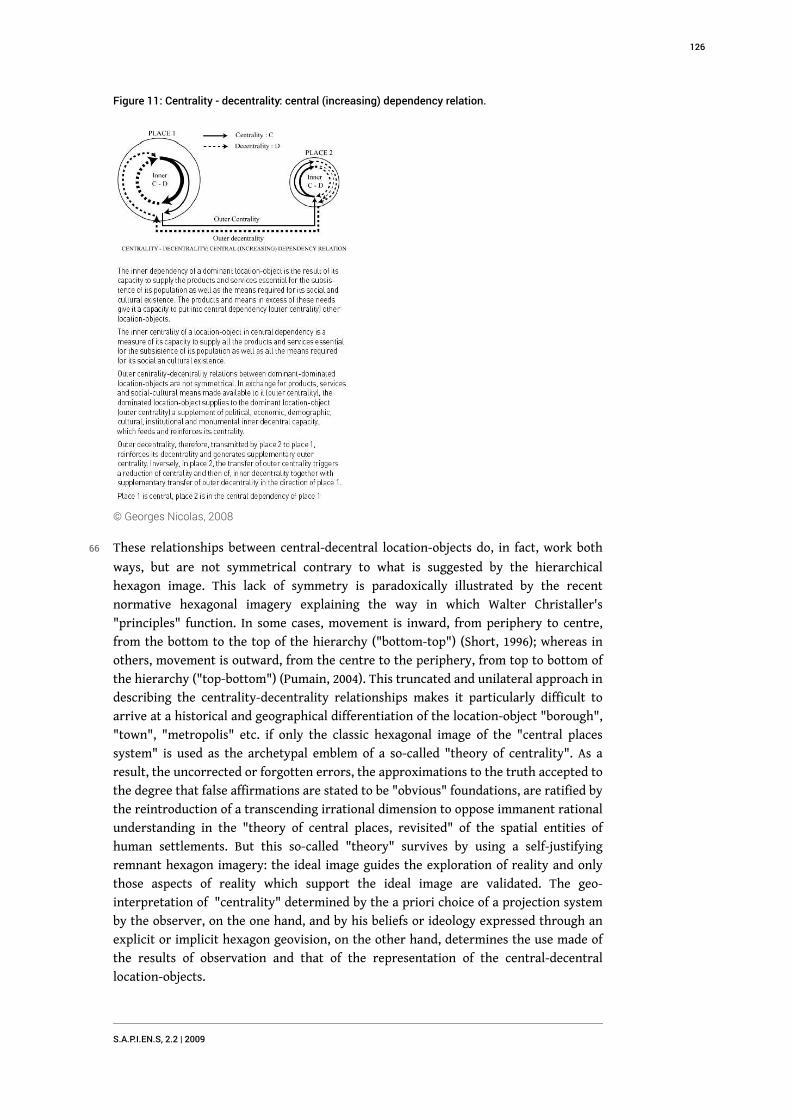
Figure 11: Centrality - decentrality: central (increasing) dependency relation.

© Georges Nicolas, 2008

66 These relationships between central-decentral location-objects do, in fact, work both

ways, but are not symmetrical contrary to what is suggested by the hierarchical

hexagon image. This lack of symmetry is paradoxically illustrated by the recent

normative hexagonal imagery explaining the way in which Walter Christaller's

"principles" function. In some cases, movement is inward, from periphery to centre,

from the bottom to the top of the hierarchy ("bottom-top") (Short, 1996); whereas in

others, movement is outward, from the centre to the periphery, from top to bottom of

the hierarchy ("top-bottom") (Pumain, 2004). This truncated and unilateral approach in

describing the centrality-decentrality relationships makes it particularly difficult to

arrive at a historical and geographical differentiation of the location-object "borough",

"town", "metropolis" etc. if only the classic hexagonal image of the "central places

system" is used as the archetypal emblem of a so-called "theory of centrality". As a

result, the uncorrected or forgotten errors, the approximations to the truth accepted to

the degree that false affirmations are stated to be "obvious" foundations, are ratified by

the reintroduction of a transcending irrational dimension to oppose immanent rational

understanding in the "theory of central places, revisited" of the spatial entities of

human settlements. But this so-called "theory" survives by using a self-justifying

remnant hexagon imagery: the ideal image guides the exploration of reality and only

those aspects of reality which support the ideal image are validated. The geo-

interpretation of "centrality" determined by the a priori choice of a projection system

by the observer, on the one hand, and by his beliefs or ideology expressed through an

explicit or implicit hexagon geovision, on the other hand, determines the use made of

the results of observation and that of the representation of the central-decentral

location-objects.

S.A.P.I.EN.S, 2.2 | 2009

126

6. The dialectic of forms in "geographic visualization"

67 External reality as an object precedes the approach by the geographer using the

differences in reality to acquire knowledge of it. Geography cannot exist without the

Earth, which is its original object. On Earth, all objects have a place, but it is impossible

to determine a priori if an object is, or is not, a geographical one. As a consequence, any

terrestrial location-object is first of all a spatial entity belonging simultaneously to two

sets: the locations set and the objects set, and each information concerns two elements

forming an indissociable pair: a location and an object. The sets of locations and objects

form a Cartesian product; meaning that the elements of these sets form distinct

ordered pairs, each pair made up of a location and an object. The specific geographic

differentiation of information [related to general differentiation (in French :

différenciation) but distinct from mathematical differentiation (in French :

différentiation)] related to a spatial entity, concerns either the location, or the object,

or both at once.

68 Geographic location-objects can be drawn on the walls of a cave, parchment, a sheet of

paper, a computer screen, etc. This way of indicating their respective positions, their

situation, makes it possible to construct a geomap, which is an artefact showing the

relations between the location-objects represented. These drawings represent directly

both differentiation by place and by object simultaneously. Historically, these drawings

of geomaps came before maps, but they are still used in the form of various geographic

diagrams: mental maps, advertisements, logos, computer graphics, cartograms, etc.

While the situation on a geomap can be either qualitative or quantitative, the

localization of a geographic location-object is achieved quantitatively using numerical

coordinates in relation to axes in a plane. The graphic representation of each locus or

object, using localization, is what is used to manufacture an artefact, called a map.

69 The object Earth can be seen as a set, considered to be a Whole. The constituent

elements of that set, the Parts, sub-sets of the Whole, are geographic objects of the 1st

order. When they are distinguished by a further property, the Parts of the Whole

become geographic objects of the 2nd order. Clearly, further developments of this

approach are going to generate Parts of successive orders (3, 4, .., n) depending on the

distinctions made as a function of the problems under consideration. Then, each

distinction leads to Parts of the Whole/s which may in turn be considered as Whole/s

and subdivided into new Parts. If a distinction leads to differentiation, this latter leads

to a spatial decomposition which generates classes of equivalence. The differentiation

of the Whole into Parts can be interpreted as an equivalence (reflexive, symmetrical

and transitive) or a tolerance relationship (reflexive and symmetrical, but not

transitive). The geographic definition of the Whole/s and of the Parts does not imply

any geodesic approach or any precise geometric figure (Nicolas and Marcus, 1997).

70 Every time a geovisualization is interpreted a posteriori using an a priori geographic

vision, this is a combination of a geomap to produce a new geomap (figure 13).

Therefore, in the case of the triangular-hexagonal geomap of the central places system,

the place "centre" and the object “hexagon” are both differentiated. As a result, it is

the "principles" attributed to the places in connection with their situation on the

vertexes, the sides or inside the triangular-hexagonal objects, which explain the spatial

relationships between location-objects. The hierarchical arrangement which emerges

S.A.P.I.EN.S, 2.2 | 2009

127

as a result is considered to be a natural or necessary order. Conversely, the map on

which is overlaid the triangular-hexagonal geomap is only differentiated by object, in

this case, the various geographic entities (functions, number of inhabitants, distances,

etc.) which are involved in the populated areas. The localization of these depends on

the projection systems which are defined a priori independently of the objects to be

represented. It is not therefore the cartographic location which explains the urban

geographic properties of the location-objects under consideration, but their "geomap"

graphic situation.

71 In practice, to verify if there is a match between the triangular-hexagonal image

considered as a "model", and urban reality to validate the "centrality theory", an a

priori geomap is overlaid onto an a posteriori map, considered to be an "outline map"

or "base map". If it can be deduced that the "triangular-hexagonal model" is still

applicable, even if it is reduced to a verbal metaphoric interpretation of the kind

"everything seems to indicate that reality (ground truth) is in conformity with the

model", then a new location-object with special characteristics is being fabricated

(figure 13):

72 Reality = information → irregular polygons = form a posteriori,

73 Metaphor = centre → regular hexagon = form a priori.

74 The "centre" becomes a "symbolic place" of which all cartographic a posteriori

representations — even if they are very or totally different from the a priori triangular-

hexagonal representation — are acceptable proof of the theory, since, as Walter

Christaller wrote: "Hence, the theory has a validity completely independent of what

reality looks like, but only by virtue of its logic and the “sense of adequacy”"

(Christaller, 1933). This assertion is reinforced by Peter Haggett for whom: "To ask for

facts and nothing but facts" is to return to the "the anarchy [sic] of regional empiricism

(Hagget, 1965) ". But it is a step too far when the omnipotence of "theory" justifies the

fabrication of "exquisite corpses" to salvage a world where manipulation and

institutional authority impose an understanding of the relationships between

populated location-objects based entirely on a "natural" or "necessary" hierarchical

central order.

S.A.P.I.EN.S, 2.2 | 2009

128

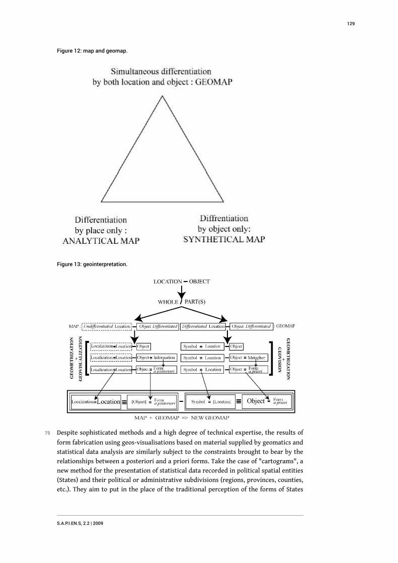
Figure 12: map and geomap.

Figure 13: geointerpretation.

75 Despite sophisticated methods and a high degree of technical expertise, the results of

form fabrication using geos-visualisations based on material supplied by geomatics and

statistical data analysis are similarly subject to the constraints brought to bear by the

relationships between a posteriori and a priori forms. Take the case of "cartograms", a

new method for the presentation of statistical data recorded in political spatial entities

(States) and their political or administrative subdivisions (regions, provinces, counties,

etc.). They aim to put in the place of the traditional perception of the forms of States

S.A.P.I.EN.S, 2.2 | 2009

129

drawn according to the space they occupy on the continents, a new vision of these

forms, the shape of which is distorted by the "weight" of the variables under

consideration. This procedure, a contemporary mapmaking practice called

“anamorphosis”, has been in use since Antiquity, and is a play on perspective

(Baltrusaitis, 1984). At the outset, it is supposed by convention that an observer looking

at an image drawn on a plane surface in front of him, examines it from a viewpoint

which allows him to visualise a circular portion of the artwork. It is therefore supposed

that the eye of the beholder is situated at the summit of a cone, the circular base of

which is what is being looked at. This point, called "vanishing point" in learned books

on perspective, is perpendicular to the surface of the image. If the observer moves

away from this perpendicular axis, his perspective is distorted depending on the

direction of movement and the angle he is using. With reference to the so called

"normal" perpendicular frontal vision, perpendicular vision from above is called

"ceiling vision", and vision from below is "plunging". Finally, if two separate "vanishing

points", spaced like two eyes, are used, vision is "bifocal" (Dalai Emiliani, 1968).

76 Maps, however, are manufactured with projection methods which give all those

beholding them a "normal" vision, wherever they may be looking from. That being so,

making a cartogram entails using a special type of anamorphosis. Instead of moving

towards the top, the bottom or the sides, the user (whose point of view is supposed to

be perpendicular to the map) is offered a modified form of the geographic entity seen

in a way which depends on what is being shown. If the figures for a State's population is

broken down into its administrative and political spatial entities - (the borough, the

parish, etc.), those whose territory is "large" are shown with a "larger" surface if they

have a large population, whereas those with few inhabitants end up with a "smaller"

surface. The effect is identical if the spatial entity is "small": its gets "less small" or

"smaller". As a result, in terms of area, the shape of large highly populated boroughs

"grow" and squeeze out of shape those which are smaller or less populated. But, to

avoid having the map "bursting out" in all directions, the external borders of the State

are unchanged, so that its initial "shape" is retained, albeit deformed. Consequently,

due to a "weighted cartographic transformation" (Cauvin, 1997; Cauvin, and Reymond,

1986), cartograms modify the surfaces of spatial entities so as to make them

proportional to a quantitative variable but keeping them with a coherent Whole: the

territory of the State concerned (Andrieu, 2005).

77 To be more precise, a cartogram is manufactured using the "barycentre" (Bouvier,

George and Le Lionnais, 1996) of the form of the spatial entity in which a numeric value

for a measured variable has been entered, using an identical surface unit for the whole

of the cartogram. Since, furthermore, the observer keeps a "normal" vision position for

each spatial entity, perpendicular to the representation plane, the "centeredness"

effect is reinforced. For those who favour cartograms, intuitive understanding of them

is easier for an untutored observer, unused to working with ordinary maps, than it is

for professional users. Even if this has not been verified by tests performed on a

sufficient number of users, the cartogram promoters are continuing to use

"hypercentration" to make them because they believe that this is scientifically

justified. This "hypercentration" is also found elsewhere, not just in cartograms

centred on a country such as France (Andrieu, 2005)39, but also in cartograms "centred"

on the world (Dodge, McDerby and Turner, 2008).

S.A.P.I.EN.S, 2.2 | 2009

130

78 One of the more sophisticated methods for producing cartograms uses diffusion

equations in molecular physics (Gastner and Newman, 2004). It was used to produce 366

cartograms using variables collected by several United Nations agencies (United Nation

Development Program, World Health Organization, United Nations Statistics Divisions)

in all the world's States (Newman and al., 2006). The starting point is a cylindrical

equidistant projection map, the central axis of which is the Greenwich meridian (figure

14). The States represented individually are grouped into 12 subsets generating Whole/

s by contiguity, although they do not constitute homogenous geopolitical units: Norway

and Switzerland are included in Western Europe defined on the basis of the European

Union, Turkey is part of Eastern Europe and Russia is in the Middle East with the Arab

countries! Each variable is related to a State with a territory whose shape is deformed

as a function of the absolute value of that variable. The result provides a visual

comparison of the various States for each of the variables chosen.

79 A great deal of research would be possible using this considerable volume of material,

all the more so since the Worldmapper website is free of access. Two of its creators

used it to evaluate by comparison in what measure the equality in Article of the 1948

Universal Declaration of Human Rights: "All human beings are born free and equal in

dignity and rights." is respected in today's world (Barford and Dorling, 2008). For the

authors, this equality signifies that all over the surface of the Earth, men and women

with equal ability, aptitude or competence should have equal chances, opportunities

and respect. The variables are the following: 1) children (births, diseases, work,

education) 2) gender equality (motherhood, contraception, employment); 3) work

(agriculture, industry, services; 4) standard of living (daily purchasing power in US

dollars); 5) travel (tourism, air passengers); 6) macro-economics (imports, exports,

levies); 7) access to information (the Internet). All the cartograms reveal severe

inequalities in contradiction with the equality set out in the Universal Declaration of

Human Rights. Their conclusion is that: " Visualization […] obliges us [English-

speaking nations and others where many have English as a second language] to

consider what is corrupt, immoral and profane about how life has come to be so

ordered, so cheap and so unjust. " (Barford and Dorling, 2008). For the two writers, as

for all the producers of Worldmapper, cartograms are therefore an objective and

effective method of raising collective awareness, thanks to the "democratization of

mapping"(Unwin, 2008). "Often our ideas about the world are based primarily on more

nebulous material that might include stereotypes, news reports and personal accounts.

These maps [cartograms] add to that and our imagination of the world because, rather

than picking out a few stories of interest, they attempt to find a space for everyone

living in the world. (Barford and Dorling, 2008) ".

80 That being so, as in the case of Christallerian centrality, there is in fact a conflict

between an a priori geovision and an a posteriori geo-visualization. To verify this, we

can try and imagine what shapes we would arrive at if "equal chances, opportunities

and respect" were achieved: the initial shape of a State would coincide with the shape

generated by the absolute value of the represented variable and there would be no

distortions, or only minimal distortion, when changing variables. Therefore, there is

indeed an a priori shape opposed in each cartogram to the a posteriori shape obtained

by graphic processing. It is the "a posteriori abnormality" of the fact represented which

deforms the a priori normality of the ideal. But the manner in which purchasing power

is calculated gives a clear indication of what "normality" is. "In Indonesia US$ 10 buys

S.A.P.I.EN.S, 2.2 | 2009

131

more than it does in the United States, so comparing earning in US$ alone does not

allow for the cost of living changing between places. The map shows purchasing power

parity (PPP) – what someone earning PPP US$ 10 would buy in the United States

"(Barford and Dorling, 2008). Cartograms 158 and 159 (figure 15) shows shapes which

are all equally monstrous: on the one hand the abnormality of the "excessively rich"

(United States: cartogram 158 and, on the other hand, the abnormality of the

"excessively poor" (India: cartogram 179). While these considerations are in agreement

with the authors' egalitarian ideals, it is not certain that they are in phase with the

needs of the "excessively poor". They make their purchases where they are and not in

the United States and they are more minded about the possibility of getting enough

food than of buying goods at American prices. The generous way in which the authors

set out the problems does indeed evidence well-documented scandalous injustice, but

they are formulated in terms and in language which are primarily addressing English-

speaking internet users, in other words, the "excessively rich".

81 The analogy between the dialectics of the shapes generated by the "Christallerian"

representations on the one hand and the Worldmappers' representations is striking: 1)

hypercentration of the representation; 2) opposition between the "ideal" geovision and

the "real" geovizualisation. And yet, the "ideals" could hardly be more opposed: on the

one side a pyramidal central hierarchic order with totalitarian excesses, on the other,

an egalitarian central order with populist excesses.

Table 3:Conclusion: Is the “Centre” a toxic concept in geography?

7. Conclusion: Is the "Centre" a toxic concept ingeography?

82 Not all the current "computer-graphics" methods experience such critical geo-

interpretation problems, generated by the dialectic between shape geovisualizations

and geovisions, as the Worldmapper cartograms. But none of them are entirely exempt

from the dangers of determination or subversion of its shapes by geovisions, as in the

case of the so-called "theory of centrality" or of the "central places system". In fact, as

we have been recently reminded, adding coordinates to a table of data does not

amount to adding two supplementary columns of variables: "Yet experience suggests

that, although the techniques used might look much the same as those used in more

general scientific visualization, there is actually something that is special about “geo”

[…] but I suspect it is also to do with the ubiquitous presence in the real world of spatial

S.A.P.I.EN.S, 2.2 | 2009

132

autocorrelation [or] what, for want of a better word, I call “context (Unwin, 2008).” All

the more since what is missing is a "well found theory to enable us to answer basic

visualization questions such as "what works?" and even "what's likely to be the best

way of displaying these data?". As a result, in the so-called "social" sciences, there is no

theory with which to test the purely spatial theories using shapes drawn from

"computer-graphics".

83 Because, contrary to what is generally stated, a "map" is not a "geomap". Today, in the

majority of cases and contrary to what was done for many centuries, mapmaking

generally precedes the production of geomaps and, furthermore, geomaps are overlaid

onto "base maps". With the absence of any theory regarding the geographic

significance of "computer visualization", there is the added confusion between

cartography (which deals with differentiation by object) and geomapgraphy (which

deals with differentiation by place and by object), so that the system is systematically

skewed in favour of geovisions using places to the detriment of geovizualisation using

localization.

84 Furthermore, the authoritative sway of very ancient metaphors and of their symbols in

geovisions tends to paralyse critical faculties to such an extreme that there is blindness

in the face of pseudo-scientific theories. A full half-century elapsed before the

elementary mathematical errors made by Walter Christaller, August Lösch and Brian

Joe Lobley Berry were discovered. How long will it be before are discovered those which

may have slipped in to the sophisticated and mathematically complex procedure of

"computer-graphics"? How many "exquisite corpses" will again be fabricated if the

discourse of geographers continues to be poisoned by as toxic a concept as the

"centre"?

Figure 14: worldmapper: land area (map 1). Each territory’s size on the map is drawn according toits land area.

Worldmapper. The world as you’ve never seen it before. Maps by Mark Newman, data by DannyDorling, text by Anna Barford, quality control by Ben Wheeler, website by John Pritchard and posterdesign by Graham Allsopp.

© Copyright 2006 SASI Group (University of Sheffield) and Mark Newman (University of Michigan).

S.A.P.I.EN.S, 2.2 | 2009

133

Figure 15: purchasing power (maps 158 and 179)

Worldmapper. The world as you’ve never seen it before.Maps by Mark Newman, data by DannyDorling, text by Anna Barford, quality control by Ben Wheeler, website by John Pritchard and posterdesign by Graham Allsopp.

© Copyright 2006 SASI Group (University of Sheffield) and Mark Newman (University of Michigan).

BIBLIOGRAPHY

Andrieu, D. (2005). L’intérêt de l’usage des cartogrammes : l’exemple de la cartographie de

l’élection présidentielle française de 2002. Mappemonde. 77(1), [On line] URL : http://

www.webcitation.org/5lVSp5o0Y.

Aujac G. (1993). Claude Ptolémée astronome, astrologue, géographe : connaissance et

représentation du monde habité. Paris, 427 pp.

Bailly, A. S. (1975). L’organisation urbaine. Théorie et modèles, Paris 272, pp.

Baltrusaitis, J. (1984). Anamorphoses, ou Thaumaturgus Opticus : les Perspectives dépravées.

Paris.

Barford, A. & D. Dorling (2008). Telling an old story with new maps. in : Dodge, M., M. McDerby, &

M. Turner. p. 67-107.

Baskin, C. W. (1966). Central places in southern Germany. New Jersey.

Bathelt, H. & J. Glückler (2003). Wirtschafts geographie. Ökonomische Beziehungen in räumlicher

Perspektive. Stuttgart (2e édition remaniée).

S.A.P.I.EN.S, 2.2 | 2009

134

Berry, B. J. L. (1956). Geographic aspects of the size and arrangement of urban centers : an

examination of central place theory with an empirical test of the hypothesis of classes of central

places. Washington.

Berry, B. J. L. (1967). Geography of market centers and retail distribution. New Jersey.

Blotevogel, H. H. (2002). Zum Verhältnis des Zentrale-Orte-Konzepts zu aktuellen

gesellschaftspolitischen Grundsätzen und Zielsetzungen. in Blotevogel. H. H. p. 17-23.

Blotevogel, H. H. (2002). Fortentwicklung des Zentrale-Orte-Konzepts. Hannover.

Bobek, H. (1961-1978). Atlas der Republik Österreich. Vienne, 6 vol.

Bobek, H. & M. Fesl (1978). Das System der zentralen Orte Österreichs : eine empirische

Untersuchung. Vienne.

Bobek, H. (1935). Eine neue Arbeit zur Stadtgeographie : Rezension von Walter Christaller. Die

zentralen Orte in Süddeutschland. Zeitschrift der Gesellschaft für Erdkunde zu Berlin. p. 125-130.

Bobek, H. (1927). Grundfragen der Stadtgeographie. Geographischer Anzeiger. p. 213-224 ;

republié dans Schöller, P. (1969). Allgemeine Stadtgeographie. Darmstadt, p. 195-219.

Bouvier, A., M. George & F. Le Lionnais (1996). Dictionnaire des mathématiques. Paris.

Böventer, E. (1963). Towards a united theory of spatial economic structure. Regional Science

Association. Papers, X, Zürich Congress, p. 163-187.

Breton, A. & P. Éluard (1938). Dictionnaire abrégé du surréalisme. Paris, éd. 1969 (1ère édition :

1938) http://www.webcitation.org/5lVkyp6hv.

Brunet, R. (2000). Des modèles en géographie ? Sens d'une recherche. Bulletin de la Société de

Géographie de Liège, n°2, p. 21-30.

Burghardt, A. F. (1979). The origin of the road and city network of Roman Pannonia. Journal of

Historical Geography, 5, 1, p. 1-20.

Capel, H. & J. L. Urteaga (1982). Las nuevas geografías. Barcelona.

Cauvin, C. (1997). Au sujet des transformations cartographiques de position. Cybergeo. Revue

européenne de géographie, Cartographie, Imagerie, SIG, article 15, mis en ligne le 14 janvier 1997,

modifié le 27 avril 2007. http://www.webcitation.org/5lVld6Vu6 Consultation : 22 décembre

2008.

Cauvin, C. & H. Reymond (1986). Nouvelles méthodes en cartographie. Montpellier.

CERTU (2001). Centralités dans la ville en mutation : quelles perspectives d’action pour les

pouvoirs publics ? Lyon.

Christaller, W. (1950). Das Grundgerüst der räumlichen Ordnung in Europa. Die Systeme der

europäischen zentralen Orte. Frankfurter geographische Hefte, 24, 1, p. 10-19.

Christaller, W. (1933). Die zentralen Orte in Süddeutschland. Eine ökonomisch-geographische

Untersuchung über die Gesetzmäßigkeit der Verbreitung und Entwicklung der Siedlungen mit

städtischen Funktionen. Darmstadt, 1980 (1ère édition : Jena, 1933).

Comptes rendus du Congrès international de géographie d’Amsterdam, (1938). T. II, Travaux des

sections. Section III a : Géographie humaine (Président : Prof. A. Demangeon). Séance du 21

juillet. Question 2 : Rapports fonctionnels entre les agglomérations urbaines et les campagnes

(Président : prof. A. Demangeon [Paris], président de séance : prof. C. Biermann [de Lausanne],

remplaçant).

S.A.P.I.EN.S, 2.2 | 2009

135

Clark, P. & B. Lepetit (1996). Capital cities and their hinterlands in early modern Europe.

Aldershot ; version révisée de Aerts, E. & P. Clark, Metropolitan cities and their Hinterlands in

early modern Europe. Session B-6 : Proceedings [of the] tenth International Economic History

Congress, Leuven, August 1990, Louvain, 1990.

Dalai Emiliani, M. (1968). La question de la perspective. 1960-1968, Arte, 2 (republié in : Argan, G.

C. & R. Wittkover (1990). Perspective et histoire au quattrocento. Montreuil, p. 97-117.

Davezies, L. (2008). La République et ses territoires. La circulation invisible des richesses, Paris.

Denzel, M. A. (1994). La practica della cambiatura. Europäischer Zahlungsverkehr vom 14. bis

zum 17. Jahrhundert, Stuttgart.

Derks, H.(1986) Stad en Land. Markt en Oikos (I), Amsterdam.

Derks, H. (2001) Deutsche Westforschung. Ideologie und Praxis im 20. Jahrhundert, Leipzig.

Djament, G. & M. Covindassamy (2005). Traduire Christaller en français. Textes seuils, réception,

récit de découverte, Cybergeo. Revue européenne de géographie, Epistémologie, Histoire,

Didactique, article 298, mis en ligne le 25 janvier 2005, modifié le 11 mai 2007. http://

www.webcitation.org/5lVms052L Consultation : 22 décembre 2008.

Dodge, M., M. McDerby, & M. Turner, (2008). Geographic visualization : Concepts, tools and

applications. Chichester.

Dörries, H. (1934). Rezension von Walter Christaller. Die zentralen Orte in

Süddeutschland.Geographische Zeitschrift, 40, p. 233-234.

Elmi, S. & C. Babin (1996). Histoire de la Terre. Paris (1ère éd. : 1994).

Favier, R. (1993). Les villes du Dauphiné aux XVIIe et XVIIIe siècles. Grenoble.

Fiétier, R. (1977). Histoire de la Franche-Comté. Toulouse.

Fray, J.-L. (2006). Villes et bourgs de Lorraine, réseaux urbains et centralité au Moyen Âge.

Clermont-Ferrand.

Fittkau, D. (2004). Beeinflussung regionaler Kaufkraftströmen durch den Autobahnlückenschluß

der A 49 Kassel-Gießen. Zur empirischen Relevanz der "New Economic Geography" in

wirtschaftsgeographischen Fragestellungen. Göttingen.

Gastner Michael T. & Newman, M.E.J. (2004). Diffusion-based method for producing density

equalizing maps. Proceedings of the National Academy of Sciences of the United States of

America, 101 / 20, p. 7499-7504.

Gilomen, H. J. & M. Stercken, (2001). Zentren. Ausstrahlung, Einzugsbereich und Anziehungskraft

von Städten und Siedlungen zwischen Rhein und Alpen. Zürich.

Gradmann, R. (1926). Volkstum und Rasse in Süddeutschland. Volk und Rasse, 1, p. 135-146.

Grimm, F.-D., G. Friedlein, & E. Müller (1997). Zentrensysteme in Mittel- und Osteuropa = Central

place systems in Central and Eastern Europe. No 5.3 – MO1, Berlin, Stuttgart.

Güssefeldt, J. (2003). Empirische Aspekte einiger Modelle der. New Economic Geography. im

Kontext jüngerer Entwicklungen des Einzelhandels. Die Erde, 134/1, p. 81-110.

Güssefeldt, J. (2005). Die Raumwirtschaftstheorien von Christaller und Lösch aus der Sicht von

Wirtschaftsgeographie und. New Economic Geography. Göttingen.

Haggett, P. (1965). Locational analysis in human geography. Londres.

Haggett, P. (1983). Geography : a modern synthesis. New-York.

S.A.P.I.EN.S, 2.2 | 2009

136

Haggett, P., A.D. Cliff & A. Frey (1977). Locational analysis : 1 Locational models, 2 Locational

methods. Londres.

Heuwinkel, D. (2002). Niedersachsen. in : Blotevogel, H. H., p. 151-167 Huriot, J.-M., (1994) Von

Thünen. Économie et espace, Paris.

Isard, W. et al (1960). Methods of regional analysis : an introduction to regional science.

Cambridge Mass./ Londres.

Jordan, P. (1989). Atlas Ost- und Südosteuropa - Atlas of Eastern and Southeastern Europe. Berlin,

Stuttgart.

Kegler, K. R., (2008). Walter Christaller. in Haar, I. & M. Fahlbusch, Handbuch der völkischen

Wissenschaften. Personen – Institutionen – Forschungsprogramme – Stiftungen, München.

Krugman, P. (1995). Development, Geography, and Economic Theory. Cambridge, Massachusetts.

Kunow, J. (1988). Zentrale Orte in der Germania Inferior. Archäologisches Korrespondenzblatt,

18, p. 55-67.

Lang, B. (2002). Die Untergliederung der Bundesrepublik Deutschland in strukturierte

Wirtschaftsregionen : eine empirische Untersuchung auf der Grundlage der

Raumstrukturtheorien von von Thünen. Christaller und Lösch, Frankfurt a.M.

Lepetit, B. (1988). Les villes dans la France moderne (1740-1840). Paris.

Lösch, A. (1938). The nature of economic regions. The Southern Economic Journal, 5, p. 71-75.

Lösch, A. (1944). Die räumliche Ordnung der Wirtschaft. (1ère éd. Jena, 1940 ; 2e éd. remaniée,

Jena, 1944) ; édition utilisée : Stuttgart, 1962 (reproduction du texte de 1944).

Mandelbrot, B. (1995). Les objets fractals : Forme, hasard et dimension. Paris.

Michalakis, M. & G. Nicolas (1986). Le cadavre exquis de la centralité. Eratosthène-Sphragide, 1, p.

38-87, Lausanne.

Miosga, M. (2002). Region München. in : Blotevogel, H. H., p. 143-150.

Newman, M. et al. (2006). Worldmapper. The world as you've never seen it before. © Copyright

2006 SASI Group (University of Sheffield) and Mark Newman (University of Michigan) http://

www.webcitation.org/5lVuxjdI3. consultation : 2 décembre 2008.

Nicolas, G. & S. Marcus, (1997). Logique Tout/Partie. in Nicolas, G., Géographie(s) et langage(s).

Interface, représentation, interdisciplinarité, Sion, p. 335-344. http://www.webcitation.org/

5lVwRBd8O, rubrique : publications, e-Eratosthène, consultation : 23 novembre 2008.

Nicolas, G. & A. Radeff (2002). Décentralité/centralité : ordre ou désordre ? in Gömmel, R. & M. A.

Denzel, Weltwirtschaft und Wirtschaftordnung : Festschrift für Jürgen Schneider zum 65

Geburtstag. Stuttgart, p. 265-286.

Nicolas, G., A. Radeff, & S. Adam. En préparation : Hexagones et centres.

Ohji, T. (1986). Normative approach to the study of periodic markets in south India. Jimbu-Chiri

(The human geography), 38, 4, p. 1-27.

Paelinck, J. H. P. (1988). L’équilibre général d’une économie stable. in : Ponsard, C., Analyse

économique spatiale. Paris, p. 277-319.

Pinchemel, P. & G. Pinchernel (1988). La face de la Terre, Paris.

Platon, (1975). Œuvres complètes. Tome XI, Les lois, livre V (-370, -348), Paris, 3e éd.

S.A.P.I.EN.S, 2.2 | 2009

137

Popper, K. W. (1959). The logic of scientific discovery. Londres.

Preston, R. E. (1992). Christaller’s research on the geography of administrative areas. Progress in

human geography. 16, 4, p. 523-539.

Pumain, D. & V. D. Leeuw (1998). La durabilité des systèmes spatiaux. in : Archeomedes, Des

oppida aux métropoles. Archéologues et géographes en vallée du Rhône, Paris, p. 13-44.

Pumain, D. (2004). Christaller (modèle de). Hypergeo, consultation : 19 avril 2005 http://

www.webcitation.org/5lVybZ1ju.

Pumain, D. (1982). La dynamique des villes. Paris.

Pumain, D., T. Paquot & R. Kleinschmager (2006). Dictionnaire. La ville et l’urbain, Paris.

Relieu, M. (1992) & M. Eliade (1907-1986). in : Encyclopédie philosophique universelle : Les

œuvres philosophiques. Paris, t. 2, p. 3201-3204.

Reynaud, J.-E. (1841). Villes. in : Leroux, P.-H. & J.-E.Reynaud. Encyclopédie nouvelle ou

dictionnaire philosophique, scientifique, littéraire et industriel offrant le tableau des

connaissances humaines au XIXe siècle. Par une société de savants et de littérateurs, Paris, t. 8, p.

670-687.

Riegger, R. (1971). August Lösch. In memoriam, Heidenheim.

Robic, M.-C. (2001). Walter Christaller et la théorie des lieux centraux. Die zentralen Orte in

Süddeutschland (1933). in : Lepetit, B. & C. Topalov. La ville dans les sciences sociales. Paris, p.

151-189 (texte) et p. 364-373 (notes).

Robson, B. T. (1973). Urban growth : an approach. Londres.

Rössler, M. & S. Schleiermacher (1993). Der Generalplan Ost. Hauptlinien der

nationalsozialistischen Planungs- und Vernichtungspolitik. Berlin.

Rössler, M. (1988). Géographie et national-socialisme. L’espace géographique, 17/ 1, p. 5-14.

Rössler, M. (1990). Wissenschaft und Lebensraum. Geographische Ostforschung im

Nationalsozialismus. Berlin/Hamburg.

Sauberer, M., V. Surd & E. Tomasi (1990). Ausstattung der ländlichen Siedlungen in Siebenbürgen

mit zentralen Einrichtungen = Availability of central facilities in rural settlements of

Transylvania. No 5.2 – R2, Berlin, Stuttgart.

Short, J. R. (1996). The urban order : An introduction to cities, culture, and power. Malden USA/

Oxford UK.

Sombart, W. (1930). Die drei Nationalökonomien. Geschichte und System der Lehre von der

Wirtschaft. München und Leipzig.

Staack, J. (1995). Die Klassifikation deutscher Städte nach ihrer regionalen Zentralität. Frankfurt

a.M. etc.

Stolper, W. F. (1954). August Lösch in Memoriam. in : Woglom, W. H., p. VII-XI.

Thünen, J. H., (1826-1875). Der isolierte Staat in Beziehung auf Landwirtschaft und

Nationalökonomie. Hamburg, Rostock et Berlin.

Ullman, E. (1941). A theory of location for cities. American journal of sociology, 56, p. 835-864.

Unwin, D. J. (2008). Foreword : encounters with « (geo) visualization ». in : Dodge, M., M. McDerby

& M. Turner, éds (2008). p. XI-XVI.

S.A.P.I.EN.S, 2.2 | 2009

138

Vagaggini, V. & G. Dematteis (1976). I metodi analitici della geografia. Florence.

Vanagas, J. (2003). Miesto Teorija [Théorie urbaine]. Vilnius.

Weichhart, P., H. Fassmann & W. Hesina (2005). Zentralität und Raumentwicklung. Vienne.

Wikipedia. http://www.webcitation.org/5lXbzdcbj, consultation : 27 décembre 2008.

Woessner, R. (2008). La métropole Rhin Rhône : vers l’émergence d’un territoire. Colmar.

Woglom, W. H. (1954). The economics of location, New Haven. Traduction du texte de Lösch, A.

(1944).

Zipf, G. K. (1949). Human behaviour and the principle of least effort. An introduction to human

ecology. Cambridge (Massachusetts).

NOTES

1. The letter k was introduced by August Lösch in 1940, in the first edition of Die räumliche

Ordnung der Wirtschaft. Walter Christaller only used real integers that we are designating by the

letter n in order to facilitate a comparison between his method and the one used by August

Lösch.

2. "Es schien überflüssig, die vorstehende Ergebnisse in Form von mathematischen Formeln auszudrücken ;

die mathematische Lösung ist selbstverständlich möglich und nicht schwierig"»: Christaller, Walter,

1933; p. 75. "It seems unnecessary to express in mathematical formulas the results discussed in the

previous paragraph.The possibility of mathematical expression is self-evident and is easily realized":

Baskin, Carlisle W., 1966; p. 70.

3. "The actual figure for occupation for each type of size [of central places] therefore corresponds

particularly well to the normal diagram except for places G and A ... [concerns the Nuremberg "L

system". (our italics)"

4. "Das zunächst Bemerkenswerte und das Gefüge des L-Systems Stuttgart in hohem Maße Bestimmende

ist die Tatsache, daß hier nicht 6, wie normal, sondern nur 5 L-Systeme anstoßen."

5. "Our diagram for the distribution and the size of the central places and the kinds of sizes is a

rational one, meaning that it signifies the greatest degree of rationality in the economy, the best

possible use of central installations and the smallest loss of "worth" (Wert). The economy is

actuated through a principle of the greatest degree of rationality."

6. While, after 1945, Walter Christaller dropped the idea of racial organic order, he remained

focused on an "ideal order" for Europe, veiled by its borders, administrative boundaries and

human population concentrations. He therefore suggests "that the disorder and what is opposed

to order be made recognisable, so as to propose reordering and the creation of a new order [sic].

It will then become possible to approach an ideal of order, or ideal order, a task which must be

undertaken urgently". To this end, he does not put forward natural components, but favours "the

system of historic human and social central places which are distributed over the surface of the

Earth according to precise rules and are integrated in a hierarchical system". He would like to

reorganise the central places of Europe, in which he sets aside "real metropolises" ("tatsächliche

gegenwärtige Metropolen"), the "true" geometric centres of countries ("eigentliche Mittelpunkte")

and the ideal urban sites ("Wunschbild-Metropolen"). He criticises the actual location of Paris,

London, Vienna and Berlin. He splits Switzerland into three systems with capitals in Paris, Rome

and Berlin and suggests its capital be transferred from Berne to Lucerne.

7. « In his Novum Organum, Bacon describes scientific theory as consisting of “anticipations, rash and

premature”. Certainly we might argue that most of the models put forward […] fit this description

admirably ; all are crude, all full of exceptions, all easier to refute than to defend. Why then, we must ask,

S.A.P.I.EN.S, 2.2 | 2009

139

do we bother to create models that study directly the “facts” of human geography? The answer lies in the

inevitability, the economy, and the stimulation of model building. […] In short the role of models in

geography is to codify what has gone before and excite fresh [sic] inquiry.»

In this 1965 edition, Karl W. Popper's book, The Logic of Scientific Discovery, London, 1959, is listed

in the bibliography. In the two-volume edition: Haggett, Peter, Cliff, Andrew D. and Frey, Allan,

1977, the reference to Karl W. Popper has disappeared. From that date onwards, refutation is no

longer a spatial analysis method: as with Walter Christaller and August Lösch, the model is again

superior to reality. The approach used tends once more to the "rotten confirmation" of the

dominant mode of thinking and its ideology.

8. Nor do the maps showing central places in the monumental Atlas of Central and Eastern Europe

((Jordan, Peter Pub., 1989 ss.), published later, contain the triangular-hexagonal diagrams .

(Sauberer, Michael, Surd, Vasile and Tomasi, Elisabeth, 1990; Grimm, Frank-Dieter, Friedlein,

Günter and Müller, Evelin, 1997).

9. « Zwischen dem Rang eines bereichsbildenden zentralen Ortes und der Gesamtzahl seiner

Kundenbevölkerung (=“Größe“ des Bereiches) besteht eine enge Relation. »

10. August Lösch recommends for reading Walter Christaller's "works on economic geography" and

praises his "admirable book"; Lösch, August, 1944, transl. Woglom, William H., 1954; p. 104, note 4

and p. 114, note 11.

11. "k" is nowhere to be found in Walter Christaller's publications.

12. For Walter Christaller the initial geometric figure is a triangle and not a regular hexagon. He

starts off using the figure 2 to designate the two apexes of the triangle on which he situates the

two lower places in relation to the third superior place which he situates on the third apex .

(Christaller, Walter, 1933; p. 70; trad. BASKIN, Carlisle W., 1966; p. 65). On that basis, he deduces a

geometric progression to explain how, in a system of complementary regions, the lower-order

centres fit into the hierarchy compared to the superior centres, i.e.: a number of

"complementary regions" equal to three in the "market principle", to four in the "transport

principle" and seven in the "administrative principle". (Christaller, Walter, 1933; p. 72; transl.

Baskin, Carlisle W., 1966; p. 67-68). In other words, for Walter Christaller, 3, 4 and 7 designate the

number of places directly dominated in a hexagonal pyramidal hierarchy and not the numerical

expression of a law permitting the number of places dominated to be deduced using a general

equation expressing the relationships between places of production and distribution and the

places of consumption, as is the case with August Lösch. (LÖSCH, August, 1944; p. 92, note 1;

transl. Woglom, William H.,1954; p. 131-133, note 16).

13. August Lösch considers that Walter Christaller's decision to choose hexagons in order to

study "the size and shape of […] the [economic] region" […] as "general though inadequate" (sic); Lösch,

August, 1944, transl. Woglom, William H., 1954; p. 114 and p. 114, note 11.

14. It is in fact this different orientation which makes it possible to identify and differentiate at

first glance Walter Christaller's administration principle (Christaller, Walter, 1933; fig. 5, p. 83

and fig. 6 p. 84) and August Lösch's k=7 diagram (Lösch, August, 1944; fig. 36, p. 92).

15. For a clear display of the differences between Walter Christaller and August Lösch in the

construction of the hierarchies of places, see: Bathelt, Harald & Glückler, Johannes, 2003; fig. 38,

p. 115.

16. August Lösch did not generalise Walter Christaller: he reduced him to the status of minion in

the service of a geographic "centrality" theory, apparently easier to understand and to teach

than difficult systems of "spatial economy" equations. Compromised by his participation in the

planning of deportations, exterminations and resettlements in the Eastern territories occupied

by the IIIrd Reich, then by electing to join the Communist Party in West Germany after the

second world war, Walter Christaller's interests were served by having it thought after 1945 that

he had some scientific kinship with August Lösch. All the more so, because Lösch's refusal to join

the Nazis attenuated Walter Christaller's proximity to them. August Lösch's good political

S.A.P.I.EN.S, 2.2 | 2009

140

reputation overshadowed and veiled Walter Christaller's trespasses. However, the absence of a

sufficiently documented biography of August Lösch (Riegger, Roland Ed., 1971) makes it difficult

to accept such proximity unless one's attitude is purely hagiographic (see for example: Haggett,

Peter, 1965, p. 70-71). This is reinforced in economic terms, because August Lösch saw himself as

"National-Socialist" in the meaning of the English economist Alfred Marshall when he referred to

"EconomicChivalry" (Lösch, August, 1944; p. 258, note 2; trad. Woglom, William H., 1954; p. 364,

note 2). August Lösch's hostility to John Edward Keynes (a disciple of Alfred Marshall), whom he

considered to be a theorist of "chaos", never weakens throughout his "Die räumliche Ordnung der

Wirtschaft"(Lösch, August, 1944; p. 177, note 3; p. 221, note 2 ; transl. Woglom, William H., 1954; p.

251, note 3; p. 308, note 81). August Lösch's affinities with National-Socialism were detected by:

Derks, Hans, 1986; p. 258-9, notes 77 & 78; 2001; p. 177, note 75.

17. In his 1967 publication (Berry, Brian Joe Lobley, 1967; transl. 1971), only the first "axiom"

(price varies according to distance) remains (transl. p.111); the second "axiom" (there are

internal and external limits to this distance) has been dropped (p. 110-114); the third "axiom" is

simplified; the theory is only concerned with one "central and unique product", (p. 114-117) and

no longer several goods distributed from a single central place. Only the hexagonal shape of the

figures is retained, although it is impossible to understand how they are constructed using a

single "axiom" in 1967 when three were needed in 1956.

18. The equation Werner Känzig submits to William H. Woglom to calculate August Lösch's n

"smallest possible market areas" is not: but: with a: the

distance separating the "original settlements" in abscissa: i a and in ordinate: . In table 7, p.

119, the computations in the second column are invalid: the first result is 1 and not 7, etc.

19. "If our concern is with substantial aspects of cities, rather than with probability theory per se, the

study of size distributions appears to be an elaborate maze which ends in a “cul de sac”.", p. 7;

conclusion adopted by: Pumain, Denise, 1982; p. 70 and: Lepetit, Bernard, 1988; p. 178;

Mandelbrot, Benoit, 1995: "I know of few endeavours [Human behavior and the principle of least

effort] where so many strokes of genius, projected into so many directions, are lost in as thick a

coating of weird fabrications, p. 180.

20. Equation justifying the "rule" is given piecemeal and never assembled.

21. "A consequence of changing from a one-product system to several products is that 'the

advantages of a general geometric representation are lost' (Lösch 1940, p. 86). An economic

picture painted by Lösch and Christaller's central places [...] are extremely fragile images [...].

They can only act as the starting point of "the more realistic part of theoretical reflection".

(Christaller 1933, p. 86).

22. "Wir sprechen jedoch bei der gegenseitigen Beziehung sich verändernder Elemente wohl besser von

Vorgängen – jedoch sind nicht historische konkrete Vorgänge, sondern von dem individuellen konkreten

Verlauf abstrahierte „allgemeine“, typische Vorgänge gemeint, wobei die Zeit als Abstraktum

auftritt. Diese Vorgänge stehen der Wirklichkeit also näher als die rein statischen Beziehungen, sie machen

den wirklicheren Teil der theoretischen Betrachtung aus, er sei als dynamische Theorie zusammengefasst."

23. Records of the International Geographical Congress in Amsterdam, 1938 . T. II, Section III a: Human

geography (Chairman: Prof. A. Demangeon). July 21st Session. Question 2: Functional

relationships between urban and rural settlements (Chairman: Prof. Albert Demangeon [Paris],

Session Chairman: Prof. Charles Biermann [Lausanne], acting). Transcription and translation in:

Djament, Géraldine and Covindassamy, Mandana, 2005.

24. "The economics of location, […] exhibit the characteristics of a man blessed at the same time with

originality and a sense of tradition and history."

25. In particular, his thesis supervisor Robert Gradmann (Gradmann, Robert, 1926 [not quoted by

Walter Christaller]) and Werner Sombart (Sombart, Werner, 1930 [quoted by Walter Christaller])

S.A.P.I.EN.S, 2.2 | 2009

141

who inspired his "deductive" method: Christaller, Walter, 1933 ; p. 16 ; transl. Baskin, Carlisle W.,

1966; p. 4.

26. " … die Tatsache, daß hier nicht 6, wie normal, sondern nur 5 L-Systeme anstoßen." [L :

"Landeshauptstädte", capital cities of the "Land"].See also 199, 216, 234, 232, 233, 235 and 251.

27. "…die Theorie hat eine Gültigkeit ganz unabhängig davon, wie die konkrete

Wirklichkeit aus sieht, nur kraft ihrer Logik und 'Sinnadäquanz'".transl. BASKIN,

Carlisle W., 1966; p. 4-5.

28. "Abweichungen von der Theorie…", transl. Baskin, Carlisle W., 1966; p. 5. Which is an

illustration of the opinion Walter Christaller has of the work — based on classic erudition and

description — done by his historian and geographer colleagues!

29. "… sie haben mit der Theorie selbst nichts zu tun und können vor allem auch nicht ohne weiteres als

Beweis gegen die Richtigkeit der Theorie angeführt werden." transl. Baskin, Carlisle W., 1966; p. 5.

30. After acknowledging that "he was neither the first, nor the only one, nor the best of theorists

working on the town considered as a centre of connections", Marie-Claire Robic adds her voice to

the latest campaign for the rehabilitation of Walter Christaller, initiated by some American and

German geographers. Since Walter Christaller was dealing with "administrative meshing issues

and administrative planning", his theory of central places should be "re-examined or re-

inserted" in his voluminous "scientific" production on the subject of administrative reform,

before, during and after the Nazi regime (Preston, Richard E., 1992). The violence arising out of

the implementation of Walter Christaller's ideas would not invalidate either the scientific

legitimacy of his "theory", or the beauty and simplicity of his geometric "model" (Robic, Marie-

Claire, 2001; p. 158). Walter Christaller's honesty appears as "evident" in the way in which Marie-

Claire Robic dissects map 4 of Die zentralen Orte in Süddeutschland: she reproduces it cut into two

parts, so that she can mask the five-sided irregular figure which is supposed to "verify" the six-

sided regular hexagonal theoretical diagram that Walter Christaller did not reproduce on his own

map (see figure 5). The two concentric theoretical circles, however, which are the basis for the

regular hexagonal image, that Walter Christaller inserts top right on his map and that Marie-

Claire Robic reproduces, are supposed to illustrate convincingly "the confrontation between

theory and reality ("Wirklichkeit") in the distribution of places K and B around places G in

"Southern Germany". But an examination of the half map published by Marie-Claire Robic shows

that numerous places B are to be found on the place K circles and these latter are abundant on

the place B circles. Furthermore, cutting out half of the original map enables Marie-Claire Robic

to state that there are six "metropolitan" (capitals, provincial capitals?) regions around Stuttgart,

although Walter Christaller only identified five (Robic, Marie-Claire, 2001; p. 164)! Now, if the

Stuttgart "system does contain six central places, theoretically the sum of one "central" hexagon

plus six "peripheral" hexagons adds up to seven, not six, regions. As a consequence, the

rehabilitation of Walter Christaller's pretensions to re-arrangement, despite the criminal use to

which he put them during the Second World War and his outrageous proposals to transfer

European capitals after the conflict, is reason enough to forget his scientific approximations and

errors, since the "normal" response to these lapses is that since the "model" is rationally "ideal",

anything which does not fit into it is simply a lower-order deviation from rationality. So that

Marie-Claire Robic can write "... [Die zentralen Orte in Süddeutschland] is supported by a stake in the

rationality of the social order — governed in this case by the State — to which the author has

radically (sic) and continuously contributed" (Robic, Marie-Claire, 2001; p. 188). The statement

could not be bettered: an ambitious opportunist, desperately seeking academic integration, is

presented as a "somewhat self-taught outsider" (Robic, Marie-Claire, 2001; p. 153), a champion of

authoritarian State-led spatial order improvement, borne by any political order (totalitarian or

liberal) as long as it is a "central order" ("eine zentralistische Anordnung"): Christaller, Walter, 1933;

p. 21).

S.A.P.I.EN.S, 2.2 | 2009

142

31. For August Lösch, economic settlements have a "rational location" ("vernünftiger Standort",

"rational location") which for their order, is superior to their "actual location", ("wirklicher

Standort", "actual location") : Lösch, August, 1944; p. 1; transl. Woglom, William H., 1954; p. 4.

32. See figures 2 and 4.

33. The famous August Lösch figure: " Region with equal structure k = 4 ", wrongly attributed to

Walter Christaller (Lösch, August, 1944; fig. 35, p. 92,transl. Woglom, William H., 1954;figure 35, p.

132), partially respects the 3, 9, 27 "rule of progression" for place dependence (Christaller,

Walter, 1933; p. 72, transl. Baskin, Carlisle W., 1966; p. 66-68). There are in fact, for each place G,

three dominated B places. However, if a line is drawn to join identical places K, putting them at

the vertex of a hexagon, by virtue of the "market principle" n=3, the result is a figure in which

hexagons of identical rank do not cover the entire surface (figure 9). Furthermore, at all

hierarchical place levels, the figure has triangular "holes" between hexagons jointed by their

summits and not by their sides. It is therefore impossible to pursue Christaller's numeric

progression beyond 3 because August Lösch rejects a uniform distribution according to the size

of the places: " [..] the same area will usually be the market for several goods, since there are more

products than regional sizes. But beyond the market area these goods need have nothing in common".

(Lösch, August, 1944; p. 85,transl. Woglom, William H., 1954; p. 122). In this case also, August

Lösch did not "generalise" Walter Christaller. He brought him down to the rank of an underling

authority a geographic theory of "centrality", apparently easier to represent and understand

than his own difficult rotating hexagons.

34. Using the "region" instead of the "place" paves the way for lavishing advice on "planning"

and "arranging" on the basis of offers of financial compensation between regions. That being

said, in the United States, once criteria for Federal grants became identical over the whole

country, it was no longer necessary to prepare regional applications for grants based on

comparative justification. The Regional Science Department of the University of Pennsylvania,

founded in 1956, lost its status in 1993 (Davezies, Laurent, 2008; p. 41).

35. Rather like crystals collecting into "ever-larger conglomerations" (p. 19) and forming rocks

which, as they are destroyed by erosion, accumulate in basins, sink down and are cooked by the

heat and melded so that they are reformed into new rocks. These new rocks, added to the older

continental structures, build up new continents by "accretion" (p. 25).

36. " … the hierarchy of central places is firmly retained as an image representing an ideal, that

is so deeply ingrained that its foundations are considered indestructible. […] In the presence of

this flimsy evaluation of planning, the question arises of whether [geographers] are not deprived

of some internal mechanism allowing them to abandon a path that has reached its limits and

subscribe to a new paradigm."; Bathelt, Harald et Glückler, Johannes, 2003, p. 116.

37. Rather, the problem with the German tradition must surely have been that it seemed to be about

geometry, not about economics as the increasingly dominant Anglo-Saxon mainstream understood it » :

Krugman, Paul, 1995, p. 39.

38. Despite the fact that Walter Christaller, who does not mind contradicting himself, says: "The

same good has a different range at every central place …": Christaller, Walter, 1933; p. 58; transl.

Baskin, Carlisle W., 1966; p. 53.

39. Cartogram 6 for the presidential election in 2002 - the votes of the far right.

S.A.P.I.EN.S, 2.2 | 2009

143

ABSTRACTS

In most currently available geography books, spatial representations group sets of differentiated

location-objects, which can be located (directly or indirectly) on the surface of the Earth, using

latitude, longitude and altitude, and systems projecting this surface on a map. But in fact spaces

defined with the help of cartographic projection systems are independent of the locations-

objects which are represented there. That being so, once the location-object is represented with

the aid of a projection space, the cartographic spaces which have been generated can combine

the locations-objects so that they can be seen as geometrizations, giving rise to geovisualizations.

But these geo-visualo-metrizations—presumed to be objective—can be used to formulate geo-

interpretations, determined on the one hand by the a priori choice the observer made of a

projection system and, on the other hand, by beliefs and ideologies expressed with the aid of

explicit or implicit geovisions.

One of the best-known geo-interpretations is the ideal image proposed by Walter Christaller in

1933, in which he claims to explain the central function of a location-object on the surface of the

Earth, using a geometrization of its location in a regular triangular-hexagonal system. However,

the initial geometric diagram that Walter Christaller used to solve the problem he raised is

mathematically unsound.

For Walter Christaller's direct followers, this theory is still valid and it is possible to use it to

construct "models" which remain "useful" using amputations or grafts, despite the fact that one

of the main components has been proven wrong by a description of reality. The "exquisite

corpse" method consists in putting together ideas considered to be "true", with ideas that are

known to be false, in the belief that the true will cancel out the "false" and make them come

"true".

This so-called "theory" was salvaged, by neglecting or obliterating three quarters of a century's

worth of contradiction between observation and theoretical postulates, by dint of erasing and

censoring Die zentralen Orte in Süddeutschland, by moving away from or simplifying the ideal

triangular-hexagonal "explanations", by unjustifiably bestowing diagrams by other authors upon

Walter Christaller, by inversing the logic of the "central places system" and, finally, proposing

contradictory geometric interpretations of its principles. The amputation and graft process has

continued without interruption since the end of World War II, more or less intensively at various

times depending on the geographic linguistic areas.

The view that this geometrization was objective has encouraged and consolidated ideological

geo-interpretations based on a central hexagon representation, and a "geovision" has emerged

based on authority and utility and the idea of “center” has become a toxic geographic concept.

INDEX

Subjects: Perspectives

Keywords: concept, geography, geometrizations, geovisualizations, interpretations,

representations, spatial, Christaller, center, centrality, decentrality

S.A.P.I.EN.S, 2.2 | 2009

144

AUTHORS

GEORGES NICOLAS

Honorary Professor, Université de Lausanne, 15, rue Alfred de Musset, 25300 Pontarlier,

France, e-mail : georges.nicolas7@wanadoo.fr

S.A.P.I.EN.S, 2.2 | 2009

145