University of Massachusetts Amherst University of Massachusetts Amherst

ScholarWorks@UMass Amherst ScholarWorks@UMass Amherst

Doctoral Dissertations Dissertations and Theses

August 2015

Robust Mobile Data Transport: Modeling, Measurements, and Robust Mobile Data Transport: Modeling, Measurements, and

Implementation Implementation

Yung-Chih Chen University of Massachusetts Amherst

Follow this and additional works at: https://scholarworks.umass.edu/dissertations_2

Part of the OS and Networks Commons, and the Systems Architecture Commons

Recommended Citation Recommended Citation Chen, Yung-Chih, "Robust Mobile Data Transport: Modeling, Measurements, and Implementation" (2015). Doctoral Dissertations. 352. https://doi.org/10.7275/6903261.0 https://scholarworks.umass.edu/dissertations_2/352

This Open Access Dissertation is brought to you for free and open access by the Dissertations and Theses at ScholarWorks@UMass Amherst. It has been accepted for inclusion in Doctoral Dissertations by an authorized administrator of ScholarWorks@UMass Amherst. For more information, please contact scholarworks@library.umass.edu.

ROBUST MOBILE DATA TRANSPORT:MODELING, MEASUREMENTS, AND

IMPLEMENTATION

A Dissertation Presented

by

YUNG-CHIH CHEN

Submitted to the Graduate School of theUniversity of Massachusetts Amherst in partial fulfillment

of the requirements for the degree of

DOCTOR OF PHILOSOPHY

May 2015

School of Computer Science

© Copyright by Yung-Chih Chen 2015

All Rights Reserved

ROBUST MOBILE DATA TRANSPORT:MODELING, MEASUREMENTS, AND

IMPLEMENTATION

A Dissertation Presented

by

YUNG-CHIH CHEN

Approved as to style and content by:

Donald F. Towsley, Chair

James F. Kurose, Member

Arun Venkataramani, Member

Tilman Wolf, Member

Erich M. Nahum, Member

Lori A. Clarke, ChairSchool of Computer Science

ACKNOWLEDGMENTS

I would like to express my deepest appreciation and thanks to my advisor, Profes-

sor Don Towsley, for the patient guidance, encouragement, and advice he has offered

throughout my time in UMass. I have been extremely lucky to have an advisor who

is rigorous and inspirational in mathematical modeling and experimental design. I

would also like to thank Professor Jim Kurose, who taught me how to tackle problems

with a top-down manner and how to make presentations attractive to the public.

I have also collaborated with researchers from IBM Research and Cambridge Uni-

versity through the ITA project. I would like to first thank Erich Nahum, your mon-

umental effort and help over the years have paved the rugged multipath smoother.

Thank you to Richard Gibbens, your statistical aspects of data analysis have as-

sisted me to quickly find the needle in my measurement haystack and to effectively

visualize those colossal datasets. I would also like to thank Ramin Khalili, Juhoon

Kim, Karl Fischer, and Anja Feldmann from Deutsche Telekem/TU-Berlin. I am

grateful to have you working together to explore the world of multi-source, and to

experimentally demonstrate that two heads are really better than one.

This thesis would not have been completed without the support of my family and

my fiancee, Yi-Fen. Your support and tolerance guided me through the tough times.

To my bright colleagues in the Networks Lab and friends in the CS department, who

helped me work through research and life challenges. I am also indebted to Laurie

Connors for your assistance of filing my crazy travel documents and processing endless

requests to get new cellular devices/data plans. Thank you Leeanne Leclerc for

keeping my paperwork and records on track. And finally, thank you Barb Sutherland,

your warm smiles and welcoming words always make me feel at home.

iv

ABSTRACT

ROBUST MOBILE DATA TRANSPORT:MODELING, MEASUREMENTS, AND

IMPLEMENTATION

MAY 2015

YUNG-CHIH CHEN

B.Sc., NATIONAL TSING HUA UNIVERSITY, TAIWAN

M.Sc., UNIVERSITY OF MASSACHUSETTS AMHERST

Ph.D., UNIVERSITY OF MASSACHUSETTS AMHERST

Directed by: Professor Donald F. Towsley

Advances in wireless technologies and the pervasive influence of multi-homed

devices have significantly changed the way people use the Internet. These changes

of user behavior and the evolution of multi-homing technologies have brought a huge

impact to today’s network study and provided new opportunities to improve mobile

data transport.

In this thesis, we investigate challenges related to human mobility, with emphases

on network performance at both system level and user level. More specifically, we

seek to answer the following two questions: 1) How to model user mobility in the

networks and use the model for network provisioning? 2) Is it possible to utilize

network diversity to provide robust data transport in wireless environments?

We first study user mobility in a large scale wireless network. We propose a

mixed queueing model of mobility and show that this model can accurately predict

v

both system-level and user-level performance metrics. Furthermore, we demonstrate

how this model can be used for network dimensioning.

Secondly, with the increasing demand of multi-homed devices that interact with

heterogeneous networks such as WiFi and cellular 3G/4G, we explore how to lever-

age this path diversity to assist data transport. We investigate the technique of

multi-path TCP (MPTCP) and evaluate how MPTCP performs in the wild through

extensive measurements in various wireless environments using WiFi and cellular

3G/4G simultaneously. We study the download latencies of MPTCP when using dif-

ferent congestion controllers and number of paths under various traffic loads and over

different cellular carriers.

We further study the impact of short flows on MPTCP by modeling MPTCP’s

delay startup mechanism of additional flows. As flow sizes increase, we observe that

traffic in cellular networks exhibits large and varying packet round trip times, called

bufferbloat. We analyze the phenomenon of bufferbloat, and illustrate how bufferbloat

can result in numerous MPTCP performance issues. We provide an effective solution

to mitigate the performance degradation.

Finally, as popular content is replicated at multiple locations, we develop mech-

anisms that take advantage of this source diversity along with path diversity to

provide robust mobile data transport. We demonstrate this in the context of on-

line video streaming, because of its popularity and significant contribution to Inter-

net traffic. We therefore propose MSPlayer, a client-based solution for online video

streaming that adjusts network traffic distribution over each path to network dynam-

ics. MSPlayer bypasses the deployment limitations of MPTCP while maintaining

the benefits of path diversity, and exploits different content sources simultaneously.

MSPlayer can significantly reduce video start-up latency and quickly refill playout

buffer for high quality video streaming. We evaluate MSPlayer’s performance through

YouTube.

vi

TABLE OF CONTENTS

Page

ACKNOWLEDGMENTS . . . . . . . . . . . . . . . . . . . . . . . . . . . . . . . . . . . . . . . . . . . . . iv

ABSTRACT . . . . . . . . . . . . . . . . . . . . . . . . . . . . . . . . . . . . . . . . . . . . . . . . . . . . . . . . . . v

LIST OF TABLES . . . . . . . . . . . . . . . . . . . . . . . . . . . . . . . . . . . . . . . . . . . . . . . . . . . . x

LIST OF FIGURES . . . . . . . . . . . . . . . . . . . . . . . . . . . . . . . . . . . . . . . . . . . . . . . . . . . xi

CHAPTER

1. INTRODUCTION . . . . . . . . . . . . . . . . . . . . . . . . . . . . . . . . . . . . . . . . . . . . . . . . . 1

1.1 Roadmap of Chapter . . . . . . . . . . . . . . . . . . . . . . . . . . . . . . . . . . . . . . . . . . . . . . 11.2 Thesis Contributions . . . . . . . . . . . . . . . . . . . . . . . . . . . . . . . . . . . . . . . . . . . . . . 21.3 Thesis Outline . . . . . . . . . . . . . . . . . . . . . . . . . . . . . . . . . . . . . . . . . . . . . . . . . . . 4

2. MOBILITY MODELING FOR LARGE SCALE WIRELESSNETWORKS . . . . . . . . . . . . . . . . . . . . . . . . . . . . . . . . . . . . . . . . . . . . . . . . . . . 5

2.1 The Traces . . . . . . . . . . . . . . . . . . . . . . . . . . . . . . . . . . . . . . . . . . . . . . . . . . . . . . 6

2.1.1 Trace Description . . . . . . . . . . . . . . . . . . . . . . . . . . . . . . . . . . . . . . . . . . 62.1.2 Trace Preprocessing . . . . . . . . . . . . . . . . . . . . . . . . . . . . . . . . . . . . . . . . 7

2.1.2.1 Departure Length Threshold . . . . . . . . . . . . . . . . . . . . . . . . . 72.1.2.2 The Observation Period . . . . . . . . . . . . . . . . . . . . . . . . . . . . . 92.1.2.3 Multiple Associations . . . . . . . . . . . . . . . . . . . . . . . . . . . . . . 102.1.2.4 Ping-Pong Effect . . . . . . . . . . . . . . . . . . . . . . . . . . . . . . . . . . 11

2.2 The Model . . . . . . . . . . . . . . . . . . . . . . . . . . . . . . . . . . . . . . . . . . . . . . . . . . . . . . 11

2.2.1 Open Class . . . . . . . . . . . . . . . . . . . . . . . . . . . . . . . . . . . . . . . . . . . . . . . 122.2.2 Closed Class . . . . . . . . . . . . . . . . . . . . . . . . . . . . . . . . . . . . . . . . . . . . . . 152.2.3 Mixed Queueing Network . . . . . . . . . . . . . . . . . . . . . . . . . . . . . . . . . . . 15

2.3 Model Validation . . . . . . . . . . . . . . . . . . . . . . . . . . . . . . . . . . . . . . . . . . . . . . . . 16

vii

2.3.1 AP Occupancy Distribution . . . . . . . . . . . . . . . . . . . . . . . . . . . . . . . . 162.3.2 User-level Performance Analysis . . . . . . . . . . . . . . . . . . . . . . . . . . . . . 18

2.3.2.1 Mean Sojourn Time . . . . . . . . . . . . . . . . . . . . . . . . . . . . . . . 182.3.2.2 Average Path Length . . . . . . . . . . . . . . . . . . . . . . . . . . . . . . 19

2.4 Applications and Network Dimensioning . . . . . . . . . . . . . . . . . . . . . . . . . . . . 192.5 Related Work . . . . . . . . . . . . . . . . . . . . . . . . . . . . . . . . . . . . . . . . . . . . . . . . . . . 212.6 Conclusion . . . . . . . . . . . . . . . . . . . . . . . . . . . . . . . . . . . . . . . . . . . . . . . . . . . . . 22

3. MOBILE DATA TRANSPORT WITH MULTI-PATH TCP . . . . . . . 23

3.1 Background . . . . . . . . . . . . . . . . . . . . . . . . . . . . . . . . . . . . . . . . . . . . . . . . . . . . . 25

3.1.1 Cellular data and WiFi networks . . . . . . . . . . . . . . . . . . . . . . . . . . . . 263.1.2 Multi-Path TCP . . . . . . . . . . . . . . . . . . . . . . . . . . . . . . . . . . . . . . . . . . 27

3.1.2.1 Connection and Subflow Establishment . . . . . . . . . . . . . . 273.1.2.2 Congestion Controller . . . . . . . . . . . . . . . . . . . . . . . . . . . . . . 27

3.2 Measurement Methodology . . . . . . . . . . . . . . . . . . . . . . . . . . . . . . . . . . . . . . . 30

3.2.1 Experiment Setup . . . . . . . . . . . . . . . . . . . . . . . . . . . . . . . . . . . . . . . . . 303.2.2 Experiment Methodology . . . . . . . . . . . . . . . . . . . . . . . . . . . . . . . . . . . 333.2.3 Performance Metrics . . . . . . . . . . . . . . . . . . . . . . . . . . . . . . . . . . . . . . . 34

3.3 Baseline Measurements . . . . . . . . . . . . . . . . . . . . . . . . . . . . . . . . . . . . . . . . . . . 36

3.3.1 Small Flow Measurements . . . . . . . . . . . . . . . . . . . . . . . . . . . . . . . . . . 39

3.3.1.1 Results at a glance . . . . . . . . . . . . . . . . . . . . . . . . . . . . . . . . 403.3.1.2 Simultaneous SYNs . . . . . . . . . . . . . . . . . . . . . . . . . . . . . . . 44

3.3.2 Large Flow Measurements . . . . . . . . . . . . . . . . . . . . . . . . . . . . . . . . . . 46

3.4 Latency Distribution . . . . . . . . . . . . . . . . . . . . . . . . . . . . . . . . . . . . . . . . . . . . . 48

3.4.1 Packet Round Trip Times . . . . . . . . . . . . . . . . . . . . . . . . . . . . . . . . . . 493.4.2 Out-of-order Delay . . . . . . . . . . . . . . . . . . . . . . . . . . . . . . . . . . . . . . . . 51

3.5 Discussion . . . . . . . . . . . . . . . . . . . . . . . . . . . . . . . . . . . . . . . . . . . . . . . . . . . . . . 533.6 Related Work . . . . . . . . . . . . . . . . . . . . . . . . . . . . . . . . . . . . . . . . . . . . . . . . . . . 563.7 Summary and Conclusion . . . . . . . . . . . . . . . . . . . . . . . . . . . . . . . . . . . . . . . . . 57

4. PERFORMANCE ISSUES OF MULTI-PATH TCP INWIRELESS NETWORKS . . . . . . . . . . . . . . . . . . . . . . . . . . . . . . . . . . . . . 58

viii

4.1 Background . . . . . . . . . . . . . . . . . . . . . . . . . . . . . . . . . . . . . . . . . . . . . . . . . . . . . 594.2 Experimental Setup and Performance Metrics . . . . . . . . . . . . . . . . . . . . . . . 604.3 Modeling MPTCP Delayed Startup of Additional Flows . . . . . . . . . . . . . . 624.4 MPTCP Performance Evaluation with Cellular Networks . . . . . . . . . . . . . 66

4.4.1 Understanding Bufferbloat and RTT Variation . . . . . . . . . . . . . . . . 674.4.2 Idle Spins of the Joint Congestion Controller . . . . . . . . . . . . . . . . . . 714.4.3 Flow Starvation and TCP Idle Restart . . . . . . . . . . . . . . . . . . . . . . . 74

4.5 Related Work . . . . . . . . . . . . . . . . . . . . . . . . . . . . . . . . . . . . . . . . . . . . . . . . . . . 784.6 Conclusion and Discussion . . . . . . . . . . . . . . . . . . . . . . . . . . . . . . . . . . . . . . . . 79

5. MSPLAYER: MULTI-SOURCE AND MULTI-PATH VIDEOSTREAMING . . . . . . . . . . . . . . . . . . . . . . . . . . . . . . . . . . . . . . . . . . . . . . . . . 81

5.1 Design Principles . . . . . . . . . . . . . . . . . . . . . . . . . . . . . . . . . . . . . . . . . . . . . . . . 835.2 MSPlayer Overview . . . . . . . . . . . . . . . . . . . . . . . . . . . . . . . . . . . . . . . . . . . . . . 86

5.2.1 YouTube Video Streaming . . . . . . . . . . . . . . . . . . . . . . . . . . . . . . . . . . 865.2.2 Multi-Source and Multi-Path . . . . . . . . . . . . . . . . . . . . . . . . . . . . . . . 875.2.3 Chunk Scheduler . . . . . . . . . . . . . . . . . . . . . . . . . . . . . . . . . . . . . . . . . . 88

5.3 MSPlayer Implementation . . . . . . . . . . . . . . . . . . . . . . . . . . . . . . . . . . . . . . . . 915.4 Testbed Experimentation . . . . . . . . . . . . . . . . . . . . . . . . . . . . . . . . . . . . . . . . . 92

5.4.1 Multi-Source and Multi-Path . . . . . . . . . . . . . . . . . . . . . . . . . . . . . . . 935.4.2 Chunk Scheduler . . . . . . . . . . . . . . . . . . . . . . . . . . . . . . . . . . . . . . . . . . 94

5.5 Evaluation on YouTube Service . . . . . . . . . . . . . . . . . . . . . . . . . . . . . . . . . . . . 955.6 Conclusion . . . . . . . . . . . . . . . . . . . . . . . . . . . . . . . . . . . . . . . . . . . . . . . . . . . . . 98

6. SUMMARY AND FUTURE DIRECTIONS . . . . . . . . . . . . . . . . . . . . . . 99

6.1 Thesis Summary . . . . . . . . . . . . . . . . . . . . . . . . . . . . . . . . . . . . . . . . . . . . . . . . 996.2 Future Work . . . . . . . . . . . . . . . . . . . . . . . . . . . . . . . . . . . . . . . . . . . . . . . . . . . 101

BIBLIOGRAPHY . . . . . . . . . . . . . . . . . . . . . . . . . . . . . . . . . . . . . . . . . . . . . . . . . . 103

ix

LIST OF TABLES

Table Page

2.1 Parameter descriptions of the mixed queueing model. . . . . . . . . . . . . . . . . . 12

2.2 Regression statistics of inter-arrival times . . . . . . . . . . . . . . . . . . . . . . . . . . . 14

2.3 Accuracy of model-predicted AP occupancy distributions. . . . . . . . . . . . . . 17

3.1 Cellular devices used for each carrier. . . . . . . . . . . . . . . . . . . . . . . . . . . . . . . . 31

3.2 Baseline path characteristics: loss rates and RTTs (sample mean ±standard error) of single-path TCP on a per connection basisacross file sizes. Note that Sprint has a particularly high loss rateon 512 KB downloads. Note that ∼ represents for negligiblevalues (< 0.03%). . . . . . . . . . . . . . . . . . . . . . . . . . . . . . . . . . . . . . . . . . . . . . 36

3.3 Small flow path characteristics: loss rates and RTTs (sample mean±standard error) for single-path TCP connections. Note that ∼represents for negligible values (< 0.03%). . . . . . . . . . . . . . . . . . . . . . . . . 40

3.4 Path characteristics of Amherst coffee shop: cellular network andpublic WiFi hotspot. Note that ∼ represents for negligible values(< 0.03%). . . . . . . . . . . . . . . . . . . . . . . . . . . . . . . . . . . . . . . . . . . . . . . . . . . . 44

3.5 Large flow path characteristics: loss rates and RTTs (sample mean±standard error) of single-path TCP on per connection average.Note that ∼ represents for negligible values (< 0.03%). . . . . . . . . . . . . 46

3.6 Statistics on MPTCP RTT (flow mean ±standard errors) andout-of-order (OFO) delay (connection mean ±standard errors)over different carriers. . . . . . . . . . . . . . . . . . . . . . . . . . . . . . . . . . . . . . . . . 54

3.7 Summary of Netflix video streaming. . . . . . . . . . . . . . . . . . . . . . . . . . . . . . . . 54

4.1 MPTCP delayed startup model parameter descriptions. . . . . . . . . . . . . . . . 63

5.1 Fraction of traffic over WiFi (mean ±std). . . . . . . . . . . . . . . . . . . . . . . . . . . 97

x

LIST OF FIGURES

Figure Page

2.1 Average number of sessions for various departure length threshold. . . . . . . 8

2.2 Average user arrival rate to the network over the course of 24 hours. . . . . . 9

2.3 Q-Q plot of inter-arrival time distribution against exponentialdistribution with 95% confidence interval. . . . . . . . . . . . . . . . . . . . . . . . . 13

2.4 Occupancy distributions of the most heavily loaded three APs. . . . . . . . . 17

2.5 AP occupancy with scaled up arrival rates. . . . . . . . . . . . . . . . . . . . . . . . . . . 20

2.6 AP occupancy with scaled up closed population. . . . . . . . . . . . . . . . . . . . . . 21

3.1 For 2-path MPTCP experiments, only solid-line paths are used. Theadditional dashed-line paths are included for the 4-path MPTCPexperiments. . . . . . . . . . . . . . . . . . . . . . . . . . . . . . . . . . . . . . . . . . . . . . . . . . 30

3.2 Baseline Download Time: MPTCP and single-path TCP connectionsfor different carriers. The measurements were performed over thecourse of 24 hours for multiple days. . . . . . . . . . . . . . . . . . . . . . . . . . . . . 37

3.3 Baseline: faction of traffic carried by each cellular carrier in MPTCPconnections. . . . . . . . . . . . . . . . . . . . . . . . . . . . . . . . . . . . . . . . . . . . . . . . . . 38

3.4 Small Flow Download Time: MP-4 and MP-2 represent for 4-pathand 2-path MPTCP connections, and reno represents uncoupledNew Reno multi-path TCP connections. . . . . . . . . . . . . . . . . . . . . . . . . . 39

3.5 Small Flows: fraction of traffic carried by the cellular path fordifferent file sizes. . . . . . . . . . . . . . . . . . . . . . . . . . . . . . . . . . . . . . . . . . . . . . 41

3.6 Amherst coffee shop: public free WiFi over Comcast businessnetwork. . . . . . . . . . . . . . . . . . . . . . . . . . . . . . . . . . . . . . . . . . . . . . . . . . . . . . 42

xi

3.7 Amherst coffee shop: fraction of traffic carried by the cellular path.With MPTCP-coupled and uncoupled New Reno TCPs, whereMPTCP is in favor of the cellular path when the file sizeincreases. . . . . . . . . . . . . . . . . . . . . . . . . . . . . . . . . . . . . . . . . . . . . . . . . . . . . 43

3.8 Small Flows: download time for simultaneous SYN and the defaultdelayed SYN approach. . . . . . . . . . . . . . . . . . . . . . . . . . . . . . . . . . . . . . . . 45

3.9 Large Flow Download Time: MP-4 and MP-2 represent for 4-pathand 2-path MPTCP connections, and reno represents uncoupledNew Reno multi-path TCP connections. . . . . . . . . . . . . . . . . . . . . . . . . 47

3.10 Large Flows: fraction of traffic carried by the cellular path fordifferent file sizes. . . . . . . . . . . . . . . . . . . . . . . . . . . . . . . . . . . . . . . . . . . . . . 48

3.11 Large Flows: download time of infinite backlog (file size 512 MB) foruncoupled New Reno/coupled MPTCP connections with four/twoflows. . . . . . . . . . . . . . . . . . . . . . . . . . . . . . . . . . . . . . . . . . . . . . . . . . . . . . . 48

3.12 Packet RTT distributions of MPTCP connections using WiFi andone of the three cellular paths. . . . . . . . . . . . . . . . . . . . . . . . . . . . . . . . . . 50

3.13 Out-of-order delay distributions of MPTCP connections using WiFiand one of the three cellular paths. . . . . . . . . . . . . . . . . . . . . . . . . . . . . . . 52

4.1 MPTCP flow establishment diagram. . . . . . . . . . . . . . . . . . . . . . . . . . . . . . . 62

4.2 Approximation of the expected number of received packets from thefirst flow as a function of RTT ratio. Samples are MPTCPmeasurements for different carriers of file sizes 1MB to 32MB. . . . . . . 67

4.3 Average connection RTT as a function of file sizes for differentcarriers (mean ± standard error). . . . . . . . . . . . . . . . . . . . . . . . . . . . . . . . 68

4.4 RTT evolution: one congestion avoidance cycle. . . . . . . . . . . . . . . . . . . . . . . 69

4.5 Network loss rate as a function of network storage F . . . . . . . . . . . . . . . . . . 71

4.6 MPTCP flow increment efficiency as a function of γ. . . . . . . . . . . . . . . . . . 72

4.7 Severe bufferbloat: periodic RTT inflation of the cellular flow resultsin idle restarts of the WiFi flow. . . . . . . . . . . . . . . . . . . . . . . . . . . . . . . . 77

4.8 Download time comparison: MPTCP with idle restart (RST) andpenalization (penl.) enabled/disabled. . . . . . . . . . . . . . . . . . . . . . . . . . . . 78

xii

5.1 HTTPS connection to YouTube web server: retrieving JSON objectsof video information. . . . . . . . . . . . . . . . . . . . . . . . . . . . . . . . . . . . . . . . . . . 86

5.2 Comparison of MSPlayer with WiFi and LTE for 40-sec pre-buffering(emulated). . . . . . . . . . . . . . . . . . . . . . . . . . . . . . . . . . . . . . . . . . . . . . . . . . . 94

5.3 Download times of three schedulers: Harmonic/EWMA/Ratio (top todown order) for different pre-buffering periods (right Y-axis) andinitial unit chunk sizes (left Y-axis). . . . . . . . . . . . . . . . . . . . . . . . . . . . . . 95

5.4 Pre-buffering 20/40/60 second video for single-path WiFi, LTE, andMSPlayer on YouTube. . . . . . . . . . . . . . . . . . . . . . . . . . . . . . . . . . . . . . . . . 96

5.5 Re-buffering 20/40/60 second video with HTTP byte range of sizes64/256 KB for single-path WiFi, LTE, and MSPlayer overYouTube service. . . . . . . . . . . . . . . . . . . . . . . . . . . . . . . . . . . . . . . . . . . . . . 97

xiii

CHAPTER 1

INTRODUCTION

The emergence of mobile technologies has changed the way people use the Inter-

net. With the explosive demand of multi-homed devices interacting with pervasive

heterogeneous networks, users can now access the Internet with their mobile devices

through WiFi or cellular networks anytime on the go. This thesis focuses on the

following two aspects of user mobility in the networks: 1) how to model user mobility

to better understand the network and for network provisioning? 2) how to efficiently

utilize network diversity for robust data transport in wireless environments?

1.1 Roadmap of Chapter

With the popularity of mobile devices and the ubiquitous deployment of cellular

networks, users can now access the Internet without the limit of time and space. This

change of network user behavior has brought a huge impact on the way researchers

analyze and evaluate wireless networks. Previous studies on wireless networking usu-

ally assume human moves in random walk fashion regardless of the underlying human

activities and develop models based on these assumptions [45, 54]. Therefore, mod-

eling user mobility in such networks has become a critical component when it comes

to protocol evaluation or architecture design. The major challenge is how to develop

such models in a concise way so that the models can abstract user behavior and

represent the underlying network activities for network provisioning.

When the user mobility is characterized and the underlying network is prop-

erly provisioned, the next challenge is, from user’s perspective, he/she might suffer

1

stalled or broken connections when transitioning from one wireless access point to

another. As modern mobile devices now have multiple wireless interfaces (e.g., WiFi

and cellular 3G/4G) and data can be transferred through different associated net-

works, having this path diversity can provide performance and robustness gains for

mobile data transport. We explore the technology of multi-path TCP (MPTCP) and

evaluate the performance of MPTCP in the wild through extensive measurements in

various wireless environments and under different traffic loads. We first characterize

each network where different wireless technologies are employed and discover several

performance issues of MPTCP when paths exhibit diverse characteristics. We analyze

these problems and provide solutions to mitigate the performance degradation.

When one or more of the exploited paths are congested or broken, MPTCP can

balance the load across all the paths and provide robust data transport between the

user and the destined server. However, often when the specific server is overloaded

or fails, there is little one can do to overcome the failure from that particular server

even with the multi-path technology. Since popular content is now replicated at

multiple locations in content delivery networks (CDNs) or data centers, users can

retrieve the desired content from a close-by server to reduce download latency. We

discuss the benefits of incorporating source diversity with path diversity and propose

a client-based solution for robust mobile data transport called MSPlayer. MSPlayer

leverages path diversity and can quickly adapt to link quality dynamics in wireless

environments. Moreover, this client-based solution takes advantage of source diversity

and can significantly reduce the download time and is resilient to server failures.

1.2 Thesis Contributions

The main contributions of this thesis are:

� We propose a simple mixed queueing model of mobility for a campus network

based on representing APs by infinite server queues (·/G/∞) to understand

2

how user mobility can affect network performance. We divide users into two

groups, an open class and a closed class. Users in the open class arrive to the

network according to a Poisson process, move from AP to AP, and eventually

depart the network. Users in the closed class are a fixed population, circulating

among APs and are always active and connected to the network. We validate

the model against empirical traces from a university network and show that the

model can precisely predict AP occupancy distributions, the average user stay

time in the network, and the average number of AP transitions of a mobile user.

Last, we demonstrate its use for network dimensioning.

� We evaluate the performance of MPTCP, which leverages all available wireless

interfaces between the sender and the receiver to provide robust data transport

for mobile users. We measure how MPTCP performs in the wild with wireless

environments, namely using both WiFi and cellular simultaneously. We show

the download latencies of MPTCP when transferring files of sizes ranging from

8 KB to 32 MB, with different numbers of paths, using different controllers, and

over different cellular carriers.

� We model the mechanism of current MPTCP’s delay startup of additional flows

to understand the impact of small file transfers when using MPTCP with paths

of different characteristics. We show the amount of traffic the first path can

deliver before the second path becomes available. We validate our model by

measuring the number packets over each MPTCP flow.

� We observe cellular flows in MPTCP connections normally exhibit large and

varying RTTs. This phenomenon is called bufferbloat, which exists in all major

US cellular networks we examined. We show how bufferbloat occurs and how

it can result in MPTCP performance degradation. When severe bufferbloat

occurs, we demonstrate how it can lead to MPTCP flow starvation due to

3

MPTCP’s design and kernel implementation. We propose an approach that

efficiently mitigates this performance issue.

� We design and implement a client-based, multi-source and multi-path online

video streaming solution called MSPlayer. MSPlayer bypasses the deployment

limitations of MPTCP. It requires no changes at the server side and no kernel

modifications at either the server or the client. MSPlayer utilizes path diversity

and does not suffer from middleboxes as does MPTCP. Moreover, as popular

content now has multiple replicas at different locations in the network, MSPlayer

exploits multiple video sources simultaneously for just-in-time high quality video

streaming. Unlike MPTCP, when a particular server fails or is overloaded,

MSPlayer provides robust data transport across different sources and hence

is resilient to server failure during video streaming. We evaluate MSPlayer’s

performance through YouTube.

1.3 Thesis Outline

The rest of this thesis is organized as follows. We present our mixed queueing

model of mobility in Chapter 2 to analyze system-level performance of a large scale

network and user-level performance of mobile users in the network. In Chapter 3, we

demonstrate how multi-path TCP can be used to provide robust data transport for

mobile users and measure its performance in the wireless environments. Chapter 4

models MPTCP’s delay flow startup mechanism and its impact to small file transfers

using MPTCP. We provide analyses of several MPTCP performance issues in wire-

less environments due to cellular bufferbloat and present a solution to mitigate the

performance degradation. In Chapter 5, we present MSPlayer, a client-based solution

for high quality video streaming that leverages both source and path diversities in

the networks. We conclude in Chapter 6, with a summary and discuss future research

directions emerging from this thesis.

4

CHAPTER 2

MOBILITY MODELING FOR LARGE SCALE WIRELESSNETWORKS

As wireless technologies have enabled user mobility dramatically when accessing

the Internet, understanding user mobility is therefore crucial for studying wireless

network protocols and evaluation of architecture design. Moreover, such models can

also be used for network dimensioning, answering “what if” questions, such as how

performance changes as the number of users or traffic scales up, or as the deployed

network infrastructure evolves.

In this chapter, we explore the use of mixed queueing networks to model user

mobility among access points (APs), consisting of users in an open and a closed class.

Users in the open class arrive according to a random process, move from AP to AP,

and depart the network. Users of this class might be laptop users, leaving the network

after being served in public hot spots; here, each new arrival to the campus network

is treated as a new, independent customer, considerably simplifying the computation

of performance metrics. Users in the closed class form a fixed population, circulating

among APs but never leaving the network. These customers could be users carrying

their smart phones that are always connected to campus APs, or users whose laptops

are similarly always connected.

The question we address is the following: can such a mixed queueing network

model, with its many simplifying independence assumptions, accurately predict vari-

ous measures of network-level performance (e.g., user population distribution at APs)

and user-level performance (e.g., mean sojourn time and average path length) in the

wireless network?

5

Starting with AP-level CRAWDAD [1] traces of user-AP affiliation over time in a

campus network, and comparing model-predicted performance with the performance

actually observed in the traces, our findings here are that such a simple model of

mobility can indeed be used to accurately predict a number of performance measures

of interest. We also illustrate the application of our model in system-level performance

and dimensioning analyses.

The remainder of this chapter is structured as follows. Section 2.1 describes the

traces we use, and how we pre-process them. Section 2.2 presents our proposed

queueing network model, which is validated in Section 2.3. We show an application

of our model for network dimensioning in Section 2.4. Related work is discussed in

Section 2.5 and Section 2.6 concludes this chapter. The research described here was

published in [18,19].

2.1 The Traces

There are several publicly available traces of long term user activity in wireless

LANs (WLANs) [13, 41, 68]. As we are interested in modeling user-level mobility

among APs in larger (e.g., campus-level) wireless networks, we seek traces that contain

information on user movements in a large network (both in terms of the number of

APs and the user population) over a long period of time. The trace we use to construct

our model, and against which we will validate model predictions, is the Dartmouth

trace [41], which records wireless user activity for a 17-week period, from 11/2/2003

to 2/28/2004.

2.1.1 Trace Description

The Dartmouth trace consists of syslog events and Simple Network Management

Protocol (SNMP) polls. The syslog contains records sent from APs to a central server

whenever mobile users authenticate, associate, roam, disassociate, or deauthenticate.

6

We find, however, that the syslog is an unreliable source for observing users’ disas-

sociations from an AP - users rarely disassociate their devices from an AP manually,

and rarely shut down their laptops gracefully (which results in explicit deauthentica-

tion). Therefore, the exact timing of a user’s departure from the network cannot be

determined on the basis of the syslog alone. The SNMP trace, on the other hand,

passively records useful related information. The wireless LAN’s mobility controller

(i.e., a central server that coordinates all APs on campus) polls each AP every five

minutes. In response to each such SNMP poll, an AP reports to the controller those

clients that are currently associated with that AP. Although this information still

does not provide the precise time of a user’s departure from an AP, we can estimate a

user’s departure time by that user’s absence in a subsequent poll, as discussed below.

2.1.2 Trace Preprocessing

To circumvent the problem of diurnal user behavior (people’s daytime and night-

time behaviors are different), we only consider user activity during those periods of

time when the university is most active. Hence, we extracted traces from 9 AM to 5

PM of each day (as will be discussed below), and removed all weekend, holiday, and

inter-session periods as well. The processed trace contains 544 APs across 6 different

types of buildings (as listed in Table 2.3), with 5,715 distinct MAC addresses.

2.1.2.1 Departure Length Threshold

We define a session as the period of time during which a mobile user is contin-

uously connected to the campus network; during a session the user may move from

one AP to another. Thus, a session begins when the mobile user first associates with

an AP (not having been previously associated with an AP) and lasts until the user

disassociates from all network APs.

As discussed in Section 2.1.1, each AP periodically provides SNMP reports (at

five-minute intervals) listing those mobile users that are currently associated with that

7

Figure 2.1. Average number of sessions for various departure length threshold.

AP. Occasionally, we find that a user disappears from the every-five-minute SNMP

reports and then soon after reappears in later SNMP reports. There are three possible

explanations for this:

� The user left the network and later returned.

� The user was in motion, leaving one AP and then later associating with another

AP.

� An SNMP update was missing or lost.

Without explicit disassociations, it is difficult to determine which of these cases has

indeed occurred. To distinguish true network departures from incorrectly inferred

departures due to missing SNMP reports, we proceed as follows.

We introduce a departure length threshold, Td, such that if the user does not

appear in an SNMP report for an amount of time greater than Td, then the user is

inferred to have left the network. Thus, periods of association by the same user that

are separated by the amount of time δ > Td (with no SNMP reports of that user

during the intervening δ) are considered to be two separate sessions for that user.

8

Figure 2.2. Average user arrival rate to the network over the course of 24 hours.

Figure 2.1 plots the average number of sessions per-day per-user as a function

of the departure length threshold. We note a sharp drop in the average number of

sessions when the departure length threshold is less than 10 minutes (corresponding to

an absence of that user in one or two back-to-back SNMP reports), and then a much

slower decrease for larger threshold values. Thus, we chose a value of the departure

length threshold of 10 minutes, and consider a user to have remained in the network

if two intervals of activity (as reported by SNMP association reports) for that user

are separated by 10 minutes or less.

2.1.2.2 The Observation Period

Since we are interested in the period of time that the campus network is most

active, we examine the trace during the time that there are a relatively large number

of users in the network, and the network is relatively stable and stationary. Figure 2.2

plots the average weekday user arrival rate to the network at different times of day,

averaged over the entire measurement period. We note that the user arrival rate to

the network increases sharply between 6 AM to 9 AM, and remains relatively stable

9

until 5 PM, and then slowly decreases till 6 AM the next morning. Thus, we chose to

model user activity during the weekday hours of 9 to 5, as discussed above.

We also found a not-insignificant fraction of users who were present in the network

at 9 AM and remained in the network until after 5 PM (i.e., have their wireless devices

always in the connected-mode). We thus divide network users into two groups: those

present all day (9 AM - 5 PM) and those that first arrive and depart during the day.

We refer to users in the first group as being in the “closed class”, and refer to the

second group of users - those that come and go - as the “open class” of users. For

each day, we computed the population of this closed class, and found that it was

relatively stable over the entire measurement period. On average, the population of

this closed class is, N = 441.

2.1.2.3 Multiple Associations

We observe from the five-minute SNMP reports collected by the controller that

a specific user is sometimes concurrently associated with multiple APs. This occurs

when a user is associated with one AP for part of the five-minute interval, and then

a different AP (or APs) for another part of the same five minute interval. When such

conflicts occur, we assign the user to the AP that most recently reported the user as

being associated with it and remove the user from other APs for this time interval.

We process the trace from start-to-finish, sequentially applying this rule as needed.

Once we identify sessions, remove multiple associations, we are left with the prob-

lem of associating times at which users transit between APs, and leave the network.

To resolve this issue, we randomly choose the associating time from a uniform dis-

tribution across this five-minute interval. If the user has a subsequent association,

then the departure time of the first AP is set to the its associating time to the next AP.

10

2.1.2.4 Ping-Pong Effect

Last, we observe occasionally the presence of a ”ping-pong effect” - the phe-

nomenon where a wireless device associates with one AP at a time, but does not stay

with it for a while. It, instead, associates with a small, fixed set of APs [63], cycling

through them one after another and remaining for a very short period of time at each

AP. Since it is difficult to identify precisely when a user starts to exhibit the ping-

pong effect, and how many APs are involved in this effect, we do not consider this

phenomenon in this thesis. Instead, we treat each movement as a regular transition

from one AP to another.

2.2 The Model

We model the campus wireless network of APs as a mixed network where each

AP is represented by an infinite server (i.e., ·/G/∞) queue. The network is mixed in

that it serves two classes of users: a closed class and an open class. The closed class

consists of N users that always remain in the system; users in the open class arrive

according to a Poisson process and can depart the system. Since each AP is modeled

as an infinite server queue, each user (regardless of class) is served immediately (there

being an infinite number of servers) and independently of the other users1.

Before discussing the details of our model, let us first introduce the key parameters

and the notation that we will use in our model (1 ≤ i, j ≤ 544) in Table 2.1.

We will refer to the open class as class 0, and the closed class as class 1. Since

each AP is modeled as an infinite server queue, arriving customers of both classes

are served immediately and independently. Hence, we can treat the network as a

combination of two independent networks.

1In IEEE 802.11 specification, there is no user association limit for an AP. However, in practice,most AP manufactures have recommendations for AP maximum capacity.

11

Parameter Description

U total number of users at steady stateM total number of APs on campusN total number of users in closed classUi number of users associated with APi

1/µi the expected user residence time at APiλi arrival rate to APiρi load of APi, where ρi = λi/µiγi exogenous arrival rate to APipij empirical probability of an open class user moving from APi to APjvi fraction of time of a closed class user visits APi

Table 2.1. Parameter descriptions of the mixed queueing model.

2.2.1 Open Class

According to our observations, most of the exogenous arrivals to APs can be

characterized by Poisson processes, and we hence model each AP for the open class

as an M/G/∞ queue (i.e., an infinite server queue with Poisson arrivals and general

service time). It is known that the output of an M/G/∞ queue is Poisson, and the

aggregation of Poisson processes is still a Poisson process [69]. Here we assume that

user arrivals to each AP is a Poisson process, and the aggregation of these arrivals

(i.e., arrivals to the campus network) can be also characterized as Poisson process.

We validate this assumption by showing a good match between the empirical user

inter-arrival time distribution and the exponential distribution, which is characteristic

of a Poisson process.

We first look at daily arrivals to the campus network, and show that the inter-

arrival times can be well fitted by an exponential distribution. As a standard statis-

tical measure in regression analysis, we use R2 (the square correlation) to quantify

how well our samples are fitted by corresponding exponential distributions2.

2R2 is a statistical measure of how well a regression line approximates real data points and0 ≤ R2 ≤ 1. The closer R2 approaches 1, the better the model fits the data points. Hence, R2 = 1corresponds to perfect fit [32].

12

Figure 2.3. Q-Q plot of inter-arrival time distribution against exponential distribu-tion with 95% confidence interval.

Table 2.2 presents that the average R2 of all examined days is 0.9664. That

is, on average, 96.64% of the data variation in our daily traces is explained by a

corresponding exponential distribution [32]. Although R2 supports our assumption

that daily user inter-arrival times of the campus network is exponentially distributed,

we noticed that the campus network traffic volume varies from day to day.

Figure 2.3 is the quantile-to-quantile plot (Q-Q plot) of empirical inter-arrival

times against exponential distribution of the worst fitted day (with 95% confidence

interval and its corresponding R2 = 0.81) throughout the entire observation pe-

riod. This is mainly due to some long inter-arrival time samples appearing at the

tail (mostly during lunch time, where the amount of arrivals to campus network is

smaller). Since the main body of the sample distribution still matches the exponential

distribution well, we consider these samples as outliers.

The following question is, are these samples at the tail influential? If we were

able to remove these tail samples outside the 95% confidence interval [88] from our

daily traces, we would find, on average, 0.23% of these samples, resulting in a 0.0221

13

Exponential Fitting average value standard deviationoriginal R2 0.9664 0.1adjusted R2 0.9885 0.04

Table 2.2. Regression statistics of inter-arrival times

improvement in R2 (i.e., the adjusted R2) as shown in Table 2.2. As our goal is

to have a simple model that can well predict various performance measures, and

since removing these 0.23% samples does not affect the goodness of fit of our Poisson

assumption, we do not remove them from our daily traces.

As we have shown that the R2 statistics supports our assumption of Poisson

arrivals, we now proceed and assume, for this open class, that the exogenous user

arrivals to each AP are described by a Poisson process, and that each user’s expected

stay time at each AP comes from a general distribution. When a user associates with

an AP, he/she will be served immediately, regardless of the bandwidth each user is

allocated. Each AP behaves as if there are infinite number of servers for each queue,

and the AP can thus serve an infinite number of users3.

Let the exogenous arrivals to APi be described by a Poisson process with rate γi.

The aggregate arrival rate to APi is

λi = γi +∑j 6=i

λjpji, 1 ≤ j ≤ N. (2.1)

The probability that a user departs the system from APi is pi0 = 1−∑N

j=1 pij.

Let π0(~u) = P (U01 = u1, . . . , U0M = uM) denote the joint steady state probability

distribution of the occupancies of the APs, where ui = 0, 1, . . . and 1 ≤ i ≤ M . The

corresponding marginal user occupancy probability distribution of APi is

3In IEEE 802.11 specification, there is no user association limit for an AP. However, in practice,most AP manufactures have their recommendations for AP maximum capacity.

14

P (U0i = ui) = e−ρ0iρui0i

ui!. (2.2)

Hence, the joint steady state population probability distribution of those APs on

campus has the following product form

π0(~u) = P (U01 = u1, . . . , U0M = uM)

=∏M

i=1ρui0i e−ρ0i

ui!, ui ≥ 0; 1 ≤ i ≤M.

(2.3)

2.2.2 Closed Class

As discussed previously, since each AP in the network is modeled as a ·/G/∞

queue, user behavior of this closed class is independent of user behavior in the open

class. We can, therefore, model the AP occupancy distribution of the closed class as a

binomial distribution (since users of this class always circulate among APs and never

leave the network), and the joint distribution is given as a multinomial distribution.

As we are only interested in the marginal statistics of each AP, we only present

the marginal distribution of the user occupancy at APi as

P (U1i = ui) =

(N

ui

)vuii (1− vi)N−ui . (2.4)

Note that vi, the probability that a closed class user visits APi, can be obtained

directly from the trace, and N is the average number (to the closest integer) of

always-active users over the entire observation period.

2.2.3 Mixed Queueing Network

Our proposed mixed queueing network mobility model combines the previous open

and closed queueing network models, and the user occupancy distribution of APi is

simply the convolution of distributions of the closed and the open network

Ui = U0i + U1i. (2.5)

15

In this work, we are investigating the performance of a large scale campus network

where the population in the closed network is large, and the probability of finding a

user at APi is relatively small. Hence, we can approximate the binomial distribution

b(N, vi) by a Poisson distribution with parameter ρ1i such that ρ1i = N × vi (as

suggested in [43], we have max{vi} = 0.017 < 0.1 and N = 441 ≥ 100).

Hence, the convolution of two Poisson distributions leads to the marginal occu-

pancy distribution of APi in the mixed network with ρi = ρ0i + ρ1i such that

P{Ui = ui} ≈∑ui

k=0 e−ρ0i ρ

k0i

k!e−ρ1i

ρui−k1i

(ui−k)!

= e−(ρ0i+ρ1i)

ui!(ρ0i + ρ1i)

ui = e−ρiρuii

ui!.

(2.6)

With this simple expression for the AP occupancy distribution of users in both the

open and the closed class, in the following section, we will investigate how closely the

predictions from our model match empirically observed results.

2.3 Model Validation

We validate our model against the empirical trace data by considering the following

metrics: AP occupancy distribution, mean user sojourn time (i.e., a user’s session time

in the system), and the average number of transitions of a user during a session.

2.3.1 AP Occupancy Distribution

We first consider how well the model-predicted AP occupancy distribution matches

the empirically-observed occupancy distribution. We observe that the most heavily

loaded APs are in residential buildings, followed by academic buildings. Figure 2.4

shows the user occupancy distributions of the three most heavily loaded APs on

campus. In each plot, the dashed line is the result predicted by the model (with load,

ρi ≈ λi/µi+Nvi at APi), while the solid line is the empirical population distribution.

We note a good match between model predictions and the empirical values.

16

0 5 10 15 20 25 30

0.00

0.02

0.04

0.06

0.08

0.10

0.12

# users

pdf

empiricalmodel

0 5 10 15 20 25 30

0.00

0.02

0.04

0.06

0.08

0.10

# users

pdf

empiricalmodel

0 5 10 15 20 25 30

0.00

0.02

0.04

0.06

0.08

0.10

# users

pdf

empiricalmodel

Figure 2.4. Occupancy distributions of the most heavily loaded three APs.

To measure the closeness of the predicted results and the empirical ones, we use

the Kolmogorov-Smirnov goodness-of-fit test (K-S test). The K-S test is used to de-

termine whether a hypothesized distribution (i.e., predictions from our mixed ·/G/∞

queueing model) matches the empirical distribution, and is not sensitive to the bin-

ning of our data (in our case, the number of users), as is the Chi-square test [43].

In our study, we set the significance level of K-S tests to 0.05 (i.e., a 95% confidence

level). Table 2.3 shows the acceptance ratio of K-S tests, that the predictions of

our hypothesized model has a goodness-of-fit to the empirical distribution of AP

occupancy. Again, we note a good match between model predictions and empirically-

observed results. The overall accuracy of predictions of user population distribution

reported by K-S tests is 93.57%.

AP Type # passed K-S test # total APs Ratio

Residential 207 211 98.1%Academic 131 152 86.18%

Administrative 68 69 98.55 %Social 44 44 100%

Library 40 49 81.63%Athletic 19 19 100%

Total 509 544 93.57 %

Table 2.3. Accuracy of model-predicted AP occupancy distributions.

17

2.3.2 User-level Performance Analysis

We next analytically compare the mean sojourn time (i.e., the duration of a user’s

session length), and the average path length (i.e., the number of transitions that a

user makes before leaving the network) predictions from our model against those of

the empirical data.

We first complete the entries in the transition matrix related to the additional

state, 0, a state that models users leaving the network. We first denote the exogenous

arrival rate to the network by λ, where γ =∑M

j=1 γj. We then add p00 = 0, and

p0i = γi/γ, for i = 1, . . . ,M , as the fraction of exogenous arrivals to each AP, to the

transition matrix.

User transitions in the network are described by a Markov model. We denote by

APi the state that a user currently associates with the ith AP in the network, and by

M = {AP1, AP2, · · · , APM} the set of states in which user transitions result in their

remaining in the network such that |M| = M . We denote by AP0 the exit state.

We now use above notations to derive the expected user sojourn time and the

average path length.

2.3.2.1 Mean Sojourn Time

Let Ti be the time user spends in system given that he/she is currently at APi

(i ∈M), including the period of time staying at APi. We then have

E[Ti] =1

µi+∑j∈M

pijE[Tj]. (2.7)

Define the diagonal matrix D = diag(1/µ1, . . . , 1/µM ), and T = (E[T1], · · · ,E[TM ]).

The transition probability matrix P is of the canonical form such that the submatrix

Q = (pij), i, j ∈ M, governs the transitions of a user that moves from one AP to

another AP in the network [57]. Then (2.7) can be expressed as T = D +QT . Note

18

that the inverse of (I − Q) exists [57], and thus the mean system stay time can be

computed and represented as

T = (I −Q)−1D. (2.8)

Let S be the user sojourn time, hence the mean user sojourn time of a user is

E[S] =∑i∈M

p0iE[Ti]. (2.9)

The mean sojourn time observed in the empirical data is 2.23 hours, and the corre-

sponding prediction from our analytical model is E[S] = 2.36 hours.

2.3.2.2 Average Path Length

The average path length can be easily derived using the above analysis and setting

the expected stay time at each AP to one (i.e., D = I). The average path length

observed in the empirical data is 2.07 transitions, and the corresponding prediction

from our analytical model is 2.10 transitions.

In summary, our model predicts an average path length of 2.1, which is very close

to the empirical value of 2.07. Recall that we also found that the predicted mean

sojourn time matches the empirical mean sojourn time well, with only 7.8 minutes

difference in the sojourn times, where the mean sojourn time is longer than 2 hours.

2.4 Applications and Network Dimensioning

Our proposed model can now be used to analyze the performance and dimension-

ing wireless networks. Suppose each AP has a capacity to serve K users at a time with

a guaranteed quality service, we then say that APi is overloaded if P (Ui > K) > 0.01.

That is, an AP functions properly if 99% of the time the number of users associated

with it is smaller than its capacity K. Note that in our model, both open and closed

19

AP capacity (K)

frac

tion

of o

verlo

aded

AP

s

5 10 15 20 25 30 35 40 45 50 55 60

0.1

0.3

0.5

0.7

0.9 λ

2λ3λ4λ5λ

Figure 2.5. AP occupancy with scaled up arrival rates.

class users contribute to the load, ρi, of APi (ρi ≈ ρ0i + ρ1i = λiµi

+Nvi). We assume

that the mobility of mobile users (i.e., 1/µi and vi) does not change in our study.

We first look at the case when the exogenous arrivals to the network increase. In

such a scenario, what is the fraction of APs that will become overloaded? Figure 2.5

shows the fraction of overloaded APs for different AP capacities (from 5 to 60) under

different levels of arrival rates. The solid line is the load and population computed

from the trace; if we seek to have a stable campus network with fewer than 5%

overloaded APs when the campus population (of the open class) increases five-fold,

then the AP capacity should be tripled.

Secondly, we investigate the case where additional smart phone users are intro-

duced to the campus network given that the exogenous arrival rate to the network

APs remains constant. Figure 2.6 shows the fraction of overloaded APs with respect

to different AP capacities at different scales of closed class population being intro-

duced, and the solid line is the load and population of the trace used. Similarly, if we

hope to have a stable campus network with fewer than 5% overloaded APs when the

closed class population increases five-fold, a doubling of AP capacity from 15 users

to 30 users will allow the campus network to run more smoothly.

20

AP capacity (K)

frac

tion

of o

verlo

aded

AP

s

5 10 15 20 25 30 35 40 45 50 55 60

0.1

0.3

0.5

0.7

N 2N 3N 4N 5N

Figure 2.6. AP occupancy with scaled up closed population.

2.5 Related Work

There are several works on modeling mobility in cellular networks. Kim and

Choi [62] developed a mobility model of cell phone users, but focused on calculating

the call handoff rate and loss probabilities in a cell for an assumed exogenous arrival

and inter-cell probabilistic mobility model. Ashtiani et al. [12] characterized spatial

traffic distribution of a fixed number of active users in a closed network to obtain

user location density in cellular networks. Both works made additional assumptions

about cell dwell time and call holding time with no supporting field data. Ghosh et

al. [35] examined traces of specific types of public Wi-Fi hotspots. They modeled

the number of users and their stay time at each hotspot, but did not consider user

mobility.

To our knowledge, this chapter presents the first analytical model with a simple

queueing model of mobility with empirical validation to predict various network and

user-level measures in a simple yet efficient manner.

21

2.6 Conclusion

In this chapter, we proposed a simple mixed queueing network model of mobility

with infinite server (·/G/∞) queues as APs on campus. We divide mobile users into

two groups, the open class and the closed class. In such a network, users in the open

class arrive to the network according to a Poisson process, move from AP to AP, and

depart the network; users in the closed class are of a fixed population, circulating

among APs, and they always remain active. We show that our model accurately

predicts the AP occupancy distribution, the average number of AP transitions a user

makes, and the mean sojourn time (of open class users) compared to results from

empirical data. We also show that our model can be used for network dimensioning,

answering “what if” questions, such as how user performance changes as the number

of users increase, and the amount of capacity that must be deployed to maintain

user-perceived performance within a specified range.

To this end, the model helps understand the network performance from a system

perspective, but lacks the information of per-connection performance. As mobile users

rarely disassociate with APs when they roam from one AP to another or go offline,

we have no precise information of their departure time. Furthermore, when roaming

between APs, users usually need to terminate previous stalled/broken connections

and then to establish a new one to resume on-going network usage. Given most

of the mobile devices now have two or more wireless interfaces (WiFi and cellular

devices), mobility impairments in one network (e.g., WiFi) may be mitigated by using

other networks (e.g. cellular). In the following chapter, we seek to explore solutions

for above issues with multi- path TCP, which leverages multiple interfaces of mobile

devices simultaneously and also keeps track of both the closed and open user activities

without breaking related connections. Moreover, congestion controller of multi-path

TCP performs dynamic load balancing among competing TCP connections, and hence

offloads traffic from congested links and overloaded networks to more available ones.

22

CHAPTER 3

MOBILE DATA TRANSPORT WITH MULTI-PATH TCP

Many users with mobile devices can access the Internet through both WiFi and

cellular networks. Typically, these users only utilize one technology at a time: WiFi

when it is available, and cellular otherwise. Research has also focused on the develop-

ment of mechanisms that switch between cellular and WiFi as the quality of the latter

improves and degrades. This results in a quality of service that is quite variable over

time. As data downloads (e.g., Web objects, video streaming, etc.) are dominant in

the mobile environment, this can result in highly variable download latencies.

In this chapter we explore the use of a promising recent development, multi-

path rate/route control, as a mechanism for providing robustness by reducing the

variability in download latencies. Multi-path rate/route control was first suggested

by Kelly [56]. Key et al. [58] showed how multi-path rate/route control provides load

balancing in networks. Han et al. [38] and Kelly & Voice [55] developed theoretically

grounded controllers that have since been adapted into Multipath TCP (MPTCP)

[31], which is currently being standardized by the IETF.

Numerous studies, both theoretical and experimental, have focused on the benefits

that MPTCP bring to long-lived flows. These studies have resulted in a number of

changes in the controller [51, 60, 89], all in an attempt to provide better fairness and

better throughput in the presence of fairness constraints. However, to date, these

studies have ignored the effect of multi-path on finite duration flows. It is well known

that most Web downloads are of objects no more than one MB in size, although

the tail of the size distribution is large. Moreover, online video streaming to mobile

23

devices is growing in popularity and, although it is typically thought of as a download

of a single large object, it usually consists of a sequence of smaller data downloads

(500 KB - 4 MB) [81]. Thus it important to understand how the use of MPTCP

might benefit such applications.

In this chapter we evaluate how MPTCP performs in the wild, using both WiFi

and cellular simultaneously. We conduct a range of experiments varying over time,

space, and download size. We utilize three different cellular providers (two 4G LTEs,

one 3G CMDA) and one WiFi provider, covering a broad range of network characteris-

tics in terms of bandwidth, packet loss, and round-trip time. To assess how effectively

MPTCP behaves, we report not only multi-path results, but also single-path results

using the WiFi and cellular networks in isolation. We report standard networking

metrics (download time, RTT, loss) as well as MPTCP specific ones (e.g., share of

traffic sent over one path, packet reordering delay). We also examine several po-

tential optimizations to multi-path, such as simultaneous SYNs, different congestion

controllers, and using larger numbers of paths.

This chapter makes the following contributions:

� We find that MPTCP is robust in achieving performance at least close to the

best single-path performance, across a wide range of network environments. For

large transfers, performance is better than the best single path, except when

the cellular network provides poor performance.

� Download size is a key factor in how MPTCP performs, since it determines

whether a subflow can get out of slow start. It also affects how quickly MPTCP

can establish and utilize a second path. For short transfers (i.e., less than 64

KB), performance is determined by the round-trip time (RTT) of the best path,

typically WiFi in our environment. In these cases, flows never leave slow start

and are limited by the RTT. For larger transfers, in the case of LTE, as down-

24

load size increases, MPTCP achieves significantly improved download times by

leveraging both paths simultaneously, despite varying path characteristics.

� Round trip times over the cellular networks can be very large and exhibit large

variability, which causes significant additional delay due to reordering out-of-

order segments from different paths. This is particularly pronounced in the 3G

network we tested. This impacts how well MPTCP can support multimedia

applications such as video.

� Using multiple flows improves performance across download sizes. For small

transfers, this is because more flows allow more opportunity to exploit slow

start. For large transfers, this is due to their ability to utilize network bandwidth

more efficiently. Connecting multiple flows simultaneously, rather than serially,

only improves the performance of small transfers, which are most sensitive to

RTT. Different congestion controllers do not appear to have a significant impact

on performance for small file transfers. For larger file transfers, we observe that

the default congestion controller of MPTCP (coupled [77]) does not perform as

well as its alternative, olia [60].

The remainder of this chapter is organized as follows: Section 3.1 provides some

background on cellular, WiFi networks, and MPTCP. We describe our experimental

methodology in Section 3.2. Section 3.3 presents an overview of our results, and

Section 3.4 looks at latency in detail. We discuss our some implications in Section

3.5, discuss about related work in Section 3.6, and conclude in Section 3.7. The

research described here was published in [20].

3.1 Background

This section provides background and basic characteristics of cellular data and

WiFi networks, and MPTCP control mechanisms needed for the rest of the chapter.

25

3.1.1 Cellular data and WiFi networks

With the emerging population of smart phones and mobile devices, to cope with

the tremendous traffic growth, cellular operators have been upgrading their access

technologies from the third generation (3G) to the fourth generation (4G) networks.

3G Services are required to satisfy the standards of providing a peak data rate of at

least 200 K bits per second (bps). The specified peak speed for 4G services is 100

Mbps for high mobility communication, and 1 Gbps for low mobility communication.

In western Massachusetts, where we perform our measurements, AT&T and Verizon

networks have their 4G Long Term Evolution (LTE) widely deployed, while Sprint

only has 3G Evolution-Data Optimized (EVDO) available.

Cellular data networks differ from WiFi networks in that they provide broader

coverage and more reliable connectivity under mobility. Furthermore, since wireless

link losses result in poor TCP throughput and are regarded as congestion by TCP,

cellular carriers have augmented their systems with extensive local retransmission

mechanisms [17], transparent to TCP, which mitigate TCP retransmissions and re-

duce the waste of precious resources in cellular networks. Although these mechanisms

reduce the impact of losses dramatically and improve TCP throughput, they come at

the cost of increased delay and rate variability.

On the other hand, WiFi networks provide smaller packet round trip times (RTTs)

but larger loss rates. Throughout our measurements, we observe that the loss rates

over 3G/4G networks are generally less than 0.1%, while those of WiFi vary from 1%

to 3%. From our observations, the average RTT for WiFi networks is about 30 ms,

while that of 4G cellular carriers usually has base RTTs of 60 ms, and can increase

by four to ten fold in a single 4G connection (depending on the carrier and the flow

sizes, see Section 3.4), and 20-fold in 3G networks. We note that, although cellular

networks in general have larger packet RTTs, in many of our measurements, WiFi is

26

no longer faster than 4G LTE, and this provides greater incentive to use multi-path

TCP for robust data transport and better throughput.

3.1.2 Multi-Path TCP

We discuss how the current MPTCP protocol establishes a connection and describe

the different type of congestion controllers used by MPTCP.

3.1.2.1 Connection and Subflow Establishment

Once an MPTCP connection is initiated and the first flow is established, each end

host knows one of its peer’s IP addresses. When the client has an additional interface,

for example, a 3G/4G interface, it will first notify the server of its additional IP

address using an Add Address option over the established subflow and send another

SYN packet with a JOIN option to the server’s known IP address. With this MPTCP-

JOIN option, this subflow will be associated with a previously established MPTCP

connection. As many of the mobile clients are behind Network Address Translations

(NATs), when the server has an additional interface, it is difficult for the server to

directly communicate with the mobile client as the NATs usually filter out unidentified

packets [80]. The server thus sends an Add Address option on the established subflow,

notifying the client of its additional interface. As soon as the client receives it, it sends

out another SYN packet with JOIN option to the server’s newly notified IP address,

together with the exchanged hashed key for this MPTCP connection, and initiates a

new subflow [31].

3.1.2.2 Congestion Controller

As each MPTCP subflow behaves as a legacy New Reno TCP flow except for the

congestion control algorithm, after the 3-way handshake, each subflow maintains its

own congestion window and retransmission scheme during data transfer, and begins

27

with a slow-start phase that doubles the window per RTT [8] before entering the

congestion avoidance phase.

We briefly describe the different congestion avoidance algorithms that have been

proposed for MPTCP. Let us denote by wi and rtti the congestion window size and

round trip time of subflow i, and denote by w the total congestion window size over

all the subflows. Also, let R be the set of all subflows.

Uncoupled TCP Reno (reno): The simplest algorithm that one can imagine

is to use TCP New Reno congestion control over each of the subflows:

� For each ACK on flow i: wi = wi + 1wi

� For each loss on flow i: wi = wi2

.

This does not satisfy the design goal of MPTCP [77], as it fails to provide congestion

balancing in the network. We use this algorithm as the baseline and refer to it as

reno.

Coupled: The coupled congestion control algorithm was introduced in [89] and

is the default congestion controller of MPTCP [31, 77]. It couples the increases and

uses the unmodified behavior of TCP in the case of a loss. The coupled congestion

control algorithm takes into account the properties of different RTTs over different

paths and works as follows:

� For each ACK on flow i: wi = wi + min( aw, 1wi

)

� For each loss on flow i: wi = wi2

The additional parameter, a, is a function of wi and rtti for all i ∈ R and is defined

in [77] as:

a =max{ wi

rtt2i}

(∑

iwirtti

)2· w. (3.1)

28

a controls the aggressiveness of the windows increase to compensate the situa-

tions where RTTs over different paths differ widely. The coupled congestion control

algorithm aims to improve throughput, balance congestion across different paths, and

be friendly to other TCP users when paths are traversing through a shared bottle-

neck [89].

OLIA: Although the coupled congestion control algorithm provides better con-

gestion balance than reno, it fails to fully satisfy the design goals of MPTCP. An

opportunistic link increase algorithm has been proposed by Khalili et al. [60] as an

alternative to the coupled algorithm:

� For each ACK on flow i: wi = wi +wi/rtt

2i

(∑p∈R wp/rttp)2

+ αiwi

� For each loss on flow i: wi = wi2

where αi adjusts the window size and is calculated as follows:

αi =

1/|Ru||B \M|

, if i ∈ B \M 6= ∅

−1/|Ru||M|

, if i ∈M and B \M 6= ∅

0 , otherwise.

(3.2)

Ru is the set of paths available to user u. Thus, i ∈ Ru is a path and |Ru| is the

number of paths available to u. M is the set of paths of u with the largest window

sizes and B is the set of the paths that are presumably the best paths for u based on

the loss rate defined in [60]. B \M is the set of elements in B but not inM, ∅ is the

empty set. Note that αi∑

i∈Ru αi = 0 and αi can be either positive or negative based

on path conditions. OLIA increases windows faster on the paths that are the best

but have small windows. The increase is slower on the paths with maximum window

sizes. Hence, OLIA satisfies the design goals of MPTCP [31] and provides optimal

load balancing [55] with minimal probing cost.

29

Figure 3.1. For 2-path MPTCP experiments, only solid-line paths are used. Theadditional dashed-line paths are included for the 4-path MPTCP experiments.

3.2 Measurement Methodology

In this section, we describe our experimental setup and discuss our methodology.

Note that all measurements were performed during March 20 to May 7 in three

different towns (Sunderland, Amherst, and Hadley) in western Massachusetts. These

towns are approximately 10 miles apart.

3.2.1 Experiment Setup

Figure 3.1 illustrates our testbed. It consists of a server residing at the Uni-

versity of Massachusetts Amherst (UMass) and a mobile client. For most of the

measurements, we focus on the 2-path scenarios (solid lines), where the client has

two interfaces activated while the server has only interface in operation. A second

interface is only active for performance comparisons between two flows and four flows.

Our server is configured as a multi-homed host, connecting via two Intel Gigabit

Ethernet interfaces to two subnets (LANs) of the UMass network. Each Ethernet

interface is assigned a public IP address and connected to the LAN via a 1 Gigabit

Ethernet cable. The mobile client is a Lenovo X220 laptop and has a built-in 802.11

a/b/g/n WiFi interface. Here we consider two types of WiFi networks: private home

WiFi networks and public WiFi hotspots. The home WiFi network is accessed by

associating the WiFi interface to a D-Link WBR-1310 a/b/g wireless router connected

to a private home network in a residential area. The home network traffic to the

30

Internet is provided by Comcast network which serves users in the same residential

community with a maximum download rate of up to 25 Mbps. Note that the actual

WiFi download speed varies according to backhaul traffic load, type of home AP

used, and user wireless interface [84]. Unless otherwise stated, we refer to a private

home network as a WiFi network. The mobile client has three additional cellular

broadband data interfaces listed in Table 3.1, and only uses them one at a time.

Table 3.1. Cellular devices used for each carrier.

Carrier Device Name Technology

AT&T Elevate mobile hotspot 4G LTE

Verizon LTE USB modem 551L 4G LTE

Sprint OverdrivePro mobile hotspot 3G EVDO

Both the server and the client are running Ubuntu Linux 12.10 with Kernel version

3.5.7 using the stable release of the MPTCP Kernel implementation [71] version v0.86.

The UMass server is configured as an HTTP server. It runs Apache2 on port 8080,

as AT&T has a Web proxy running on port 80 which removes all the MPTCP option

fields and thus does not allow MPTCP connections. The client uses wget to retrieve

Web objects of different sizes via all the available paths.

To reduce potential WiFi interference to the working wireless interface, we disable

the functionality of WiFi bandwidth sharing on both the AT&T and Sprint devices.

Furthermore, though all devices run at different frequencies, to avoid possible interfer-

ence between these electronic devices, we use USB cables to extend cellular dongles,

and use the WiFi and only one cellular device at a time. Therefore, we assume in-

terference among the devices is negligible. Throughout the measurements, cellular

reception signals of different carriers (over different places) are in the range between

-60dBm and -102dBm, corresponding to good and weak signals.

31

3.2.1.0.1 Connection parameters The default Linux TCP uses an initial slow

start threshold value (ssthresh) of infinity, and caches parameters for per-destination

TCP connections [82]. When losses occur, the ssthresh value will be reset and cached

for initialization of future TCP connections to the same destination. However, this

is shown to be harmful for short flows [50] if an earlier connection to a particular

destination encounters a sequence of losses. This is because ssthresh will be set to

a small value and all the subsequent newly open flows to that destination will have

the same small ssthresh. Hence, we configure our server such that no parameters

of previously closed TCP connections to any destination are cached. Moreover, as

we are using cellular networks in nearly loss-free environments (as will be discussed

later), a ssthresh value of infinity will lead to the case where the cellular path never

leaves slow start. The congestion window of the cellular path could then become

extremely large and hence suffer severe RTT inflation [17,52], which can degrade the

performance of MPTCP. Therefore, we set the default value of ssthresh to 64KB

for fair comparisons among different configurations and file sizes, and to mitigate the

impact of RTT inflation described above. We use Linux’s default initial window size

of 10 packets and apply TCP Selective Acknowledgement (SACK) [30].

3.2.1.0.2 Receive memory allocation As MPTCP requires a larger receive

buffer than single-path TCP for out-of-order packets from different paths and uses

a shared receive buffer, there is a potential performance degradation if the assigned

buffer is too small [80,89]. To avoid such events during our measurements, we set the

maximum receive buffer to 8 MB.

3.2.1.0.3 No subflow penalty Throughout our experiments, we observe that

the current MPTCP implementation by default monitors each flow’s bandwidth delay

product (BDP). If a particular flow has contributed too many out-of-order packets to

the receive buffer, it penalizes that flow by reducing its congestion window by half [80],

32

even though no loss has occurred. In our experiments, as the receive memory is

always large enough, this penalization mechanism can only degrade the performance

of MPTCP connections. To measure the true performance of MPTCP connections,

we remove the penalization scheme from the implementation.

3.2.2 Experiment Methodology

As the UMass server has two physical interfaces, and the client has a built-in WiFi

interface and broadband devices from three different cellular carriers, we conduct

measurements of the following configurations:

� Single-path TCP: the UMass server activates its primary interface, and the

client enables only one interface (WiFi or cellular). Thus, there are four con-

figurations in this scenario: single path WiFi TCP or single path cellular TCP

(through AT&T, Verizon, or Sprint).

� 2-path MPTCP: the UMass server activates its primary interface, while the

client enables WiFi and a cellular device. For each configuration, we run back

to back measurements of different congestion controllers described in Section

3.1.2. There are nine configurations in this scenario: client’s three settings of

two interfaces enabled (WiFi/AT&T, WiFi/Verizon, and WiFi/Sprint) to the

server’s primary interface with three congestion controller settings.

� 4-path MPTCP: for comparison purposes, we enable the server’s secondary

interface connected to a different subnet, as illustrated in Figure 3.1. There are

also a total of nine different configurations in this scenario.

As Web traffic can be short-lived or long-lived, for each configuration, the client

downloads files of different sizes from the server via HTTP. As there is no clear

distinction between short flows and long flows, in our measurements, we consider files

of sizes 8 KB, 64 KB, 512 KB, and 4 MB as small flows. For large flows, we consider

33

file of sizes 8 MB, 16 MB, and 32 MB. We also consider infinite backlog file transfers

for performance purposes (see Section 3.3.2), and here file downloads are of size 512

MB.

Since network traffic might have dependencies and/or correlation from time to

time, and from size to size, in each round of measurements, we randomize the sequence

of configurations. That is, we randomize the order of file sizes, carriers, the choices of

congestion controllers, single-path and multi-path TCP. To capture temporal effects,

for each scenario, we conduct measurements for multiple days. To mitigate possible

spatial factors, measurements were also performed at multiple locations in the same

town, and in different towns in western Massachusetts. Note that we divide a day into

four periods: night (0-6 AM), morning (6-12 AM), afternoon (12-6 PM), and evening

(6-12 PM). For each period of time at each location, we perform 20 measurements for

each configuration.

Furthermore, since cellular 3G/4G antennas have state machines for radio re-

sources allocation and management of energy consumption, the state promotion delay

(the time duration required to bring the antenna to ready state) is often longer than

a packet RTT [46, 48] and might significantly impact our short flow measurements.

Therefore, to avoid this impact, we send two ICMP ping packets to our server before

each measurement, and start the measurements immediately after the ping responses

are correctly received to ensure that the cellular antenna is in the ready state.

We collect packet traces from both the UMass server and the client using tcpdump [86],

and use tcptrace [87] to analyze the collected traces at both sides.

3.2.3 Performance Metrics

We are interested in the following performance metrics related to MPTCP and

single-path TCP:

34

Download time: As our goal is to understand how much gain mobile users obtain

from using MPTCP, for both small flows and large flows, we focus on download time

rather than bandwidth and speed of each cellular technology. We define the download

time as the duration from when the client sends out the first SYN to the server to

the time it receives the last data packet from the server. We measure download time

of a file using MPTCP and compare it with what we get if we use a single-path TCP

over the available WiFi or 3G/4G paths.

Loss rate: The loss rate is measured on a per-subflow basis. It is calculated as

the total number of retransmitted data packets divided by the total number of data

packets sent by the server on the flow. We show the average loss rate across all the

measurements of the same configuration.

Round trip time (RTT): We measure RTTs on a per-subflow basis. Denote by

Tr the server’s receive time of an ACK packet for the previous packet sent from the

server at time Ts over a subflow. RTT is measured as the difference between the time

when a packet is sent by the server and the time the ACK for that packet is received

(i.e., RTT = Tr − Ts), such that the ACK number is larger than the last sequence

number of the packet and the packet is not a retransmission [87].

Out-of-order delay: MPTCP maintains two sequence numbers for each packet,

a data (global) sequence number for the MPTCP connection and a subflow (local)

sequence number for each TCP subflow. In-order packets arriving from the same

subflow may wait in the receive buffer before their data sequence numbers become

in-order. This could be due to late arrivals of packets from other paths. Therefore,

a key performance metric of using MPTCP is to measure packet out-of-order delay

at the receive buffer before packets are ready for delivery to the application layer.

Out-of-order delay is defined to be the time difference between when a packet arrives

at the receive buffer to when its data sequence number is in-order.

35

Table 3.2. Baseline path characteristics: loss rates and RTTs (sample mean ±standard error) of single-path TCP on a per connection basis across file sizes. Notethat Sprint has a particularly high loss rate on 512 KB downloads. Note that ∼represents for negligible values (< 0.03%).

File size

64 KB 512 KB 2 MB 16 MB

Loss (%)

AT&T 0·03±0.03 0·04±0.01 0·06±0.03 0·31±0.12

Verizon ∼ ∼ 0·31±0.13 1·75±0.20

Sprint 0·37±0.16 8·76±4.8 3·93±0.34 1·64±0.01

Comcast 0·43±0.16 0·20±0.04 2·02±0.42 0·68±0.07

RTT(ms)

AT&T 70·06±2.78 104·89±3.32 138·20±5.09 126·01±5.37

Verizon 92·41±13.23 204·65±20.45 422·56±28.34 624·66±54.55

Sprint 381·29±50.80 972·4 ±84.08 1209·81±178.68 703·81±81.96

Comcast 26·81±0.43 53·08±2.20 56·83±5.71 32·65±2.05

3.3 Baseline Measurements

Figure 3.2 presents the download times of different size files over different WiFi/cellular

carriers using single-path or MPTCP. We show results for file sizes of 64 KB, 512 KB,

2 MB, and 16 MB. We perform our measurements over each of these four time periods

in a day described in Section 3.2.2 and show the aggregate results in Figure 3.2. We

use the default coupled congestion controller as the congestion control algorithm. We

use box and whisker plots to summarize our measurement results. The line inside

each box is median, the top and the bottom of each box are the first and third quar-

tiles (25% and 75%), and the ends of the whiskers are the minimum and maximum

values.

MP-carrier refers to a 2-path MPTCP connection using a particular 3G/4G cellu-

lar network and a WiFi network. SP-carrier refers to a single-path TCP connection

over a particular WiFi/3G/4G network.

36

SP WiFiSP Sprint

MP SprintSP Verizon

MP VerizonSP AT&T

MP AT&T

SP WiFiSP Sprint

MP SprintSP Verizon

MP VerizonSP AT&T

MP AT&T

SP WiFiSP Sprint

MP SprintSP Verizon

MP VerizonSP AT&T

MP AT&T

SP WiFiSP Sprint

MP SprintSP Verizon

MP VerizonSP AT&T

MP AT&T

64KB

512KB

2MB

16MB

0.1 1 5 10 50 100 150Download time with log scale (seconds)

AT&T 4G

Verizon 4G

Sprint 3G

Comcast WiFi

Figure 3.2. Baseline Download Time: MPTCP and single-path TCP connectionsfor different carriers. The measurements were performed over the course of 24 hoursfor multiple days.

For all file sizes, we observe that the file download times under MPTCP are

almost the same as those using the best single-path TCP connection available to the

user. Sometimes MPTCP outperforms the best path alone. MPTCP initiates the

connection over the WiFi network (i.e., the WiFi path is the default path).

For small flows, i.e., file sizes of 64 KB or smaller, single-path TCP over WiFi

performs the best, and MPTCP does not provide much gain using the cellular path.

This is because WiFi connections have smaller RTTs (around 30 ms) than the 3G/4G

cellular connections (60-80 ms for 4G, and 300 ms for 3G). Thus, in most small flow

cases the file transfer is complete before the cellular paths can complete their 3-way

handshakes. For slightly larger flows, we observe that single-path over WiFi is no

longer guaranteed to be the best path (in terms of download times). Instead, single-

path TCP over 4G LTE is the best choice in many instances. This is because the

cellular networks (especially the 4G LTE networks) provide almost loss free paths,

in contrast to WiFi’s roughly 1.6% loss rate (see Table 3.2). Figure 3.3 shows the

37

MP SprintMP VerizonMP AT&T

MP SprintMP VerizonMP AT&T

MP SprintMP VerizonMP AT&T

MP SprintMP VerizonMP AT&T

64KB

512KB

2MB

16MB

0 25 50 75Fraction of traffic (%)

MP AT&T

MP Verizon

MP Sprint

Figure 3.3. Baseline: faction of traffic carried by each cellular carrier in MPTCPconnections.

fraction of traffic offloaded to the cellular path for the experiments reported in Figure

3.2. We observe that MPTCP offloads traffic from the fast but lossy WiFi paths

to the not-so-fast but loss-free cellular paths. Therefore, when the file size is not

too small, MPTCP connections gain more by leveraging the cellular path. Table 3.2

provides the loss rates and RTTs (averages and standard errors) for the measurements

in Figure 3.2.

We observe that 3G networks tend to have slightly larger loss rates than 4G,

much larger minimum RTTs (200 ms), and large RTT variations (300-800 ms). Thus,

for small flows, most packets in MPTCP-Sprint connections are delivered via WiFi.

When file sizes are large and a fraction of packets have initially been scheduled through

the 3G path, it takes much longer for those packets to reach the client. In the case

where the RTT variation is large over 3G paths (up to 8-10 times greater than its

3-way handshake RTT), and a packet is identified as lost and retransmitted, it can

take a few seconds for a packet to be delivered and results in reduced performance.

Section 3.4.2 analyzes this out-of-order delay in more detail.

In the rest of this section, we provide a more detailed analysis of the performance

of MPTCP using different congestion controllers and different file sizes. For simplicity,

we focus on one cellular carrier, AT&T 4G LTE, since it exhibits the smallest RTT

38

SP WiFiSP AT&T

MP−2 AT&T (coupled)MP−4 AT&T (coupled)

MP−2 AT&T (olia)MP−4 AT&T (olia)MP−2 AT&T (reno)MP−4 AT&T (reno)

SP WiFiSP AT&T

MP−2 AT&T (coupled)MP−4 AT&T (coupled)

MP−2 AT&T (olia)MP−4 AT&T (olia)MP−2 AT&T (reno)MP−4 AT&T (reno)

SP WiFiSP AT&T

MP−2 AT&T (coupled)MP−4 AT&T (coupled)

MP−2 AT&T (olia)MP−4 AT&T (olia)MP−2 AT&T (reno)MP−4 AT&T (reno)

SP WiFiSP AT&T

MP−2 AT&T (coupled)MP−4 AT&T (coupled)

MP−2 AT&T (olia)MP−4 AT&T (olia)MP−2 AT&T (reno)MP−4 AT&T (reno)

8KB

64KB

512KB

4MB

0.05 0.1 0.5 1 5 10Download time with log scale (seconds)

MP−4 AT&T

MP−2 AT&T

SP AT&T

SP WiFi

Figure 3.4. Small Flow Download Time: MP-4 and MP-2 represent for 4-path and2-path MPTCP connections, and reno represents uncoupled New Reno multi-pathTCP connections.

variability and the most stable performance. We also utilize different WiFi networks

at different locations.

3.3.1 Small Flow Measurements

We start by analyzing the behavior of MPTCP when transferring small files. We

chose four different file sizes here (8 KB, 64 KB, 512 KB, and 4 MB) as representative

of small flows. For simplicity, we focus on one cellular carrier, AT&T 4G LTE, with

Comcast WiFi as the default path. Our goal is to 1) understand how 2-path MPTCP

performs in the wild, and 2) understand the impact of different MPTCP congestion

controllers on connection performance. For comparison purposes, we also seek to 3)

determine the benefits of using 4-path MPTCP instead of 2-path MPTCP to download

small files.

Figure 3.4 shows the download times small flows. MP-4 and MP-2 represent

MPTCP connections consisting of four and two subflows, while the congestion con-

39

Table 3.3. Small flow path characteristics: loss rates and RTTs (sample mean±standard error) for single-path TCP connections. Note that ∼ represents for negli-gible values (< 0.03%).

File size

8 KB 64 KB 512 KB 4 MB

Loss(%)

WiFi 1·0±0.5 1·6±0.4 1·4±0.2 2·1±0.2

AT&T ∼ ∼ ∼ ∼

RTT(ms)

WiFi 22·3±0.2 38·7±6.9 33·9±2.7 23·9±0.3

AT&T 60·8±0.5 64·9±0.5 73·2±2.1 140·9±1.1

troller in parentheses indicates which congestion controller is used at the server. As

an overview of baseline small flow measurements, a clear trend is, when file size in-

creases, 4-path MPTCP performs better than 2-path MPTCP, which performs better

than single-path TCP.

3.3.1.1 Results at a glance

We observe, in the case of single-path TCP, AT&T performs the worst when the

file size is small (e.g., 8 KB). This is because the 4G network has a minimum RTT of

60 ms that is larger than the file download time over single-path WiFi (see Table 3.3).

Hence, when the file size is 8 KB, MPTCP performs just as well as single-path TCP

over WiFi (SP WiFi), regardless of the number of subflows - as most of the subflows

are not utilized. Figure 3.5 presents the fraction of traffic carried by the cellular

path under MPTCP for different file sizes. For file sizes smaller than 64 KB, 4-

path MPTCP never utilizes the cellular path to deliver traffic, while 2-path MPTCP

occasionally utilizes the cellular path.

For 4-path MPTCP, since both WiFi subflows have RTTs one half or one third

the size of those of the cellular subflows, the two WiFi subflows quickly complete the

40

MP−2 AT&T (coupled)MP−4 AT&T (coupled)

MP−2 AT&T (olia)MP−4 AT&T (olia)MP−2 AT&T (reno)MP−4 AT&T (reno)

MP−2 AT&T (coupled)MP−4 AT&T (coupled)

MP−2 AT&T (olia)MP−4 AT&T (olia)MP−2 AT&T (reno)MP−4 AT&T (reno)

MP−2 AT&T (coupled)MP−4 AT&T (coupled)

MP−2 AT&T (olia)MP−4 AT&T (olia)MP−2 AT&T (reno)MP−4 AT&T (reno)

MP−2 AT&T (coupled)MP−4 AT&T (coupled)

MP−2 AT&T (olia)MP−4 AT&T (olia)MP−2 AT&T (reno)MP−4 AT&T (reno)

8KB

64KB

512KB

4MB

0 25 50 75Fraction of traffic (%)

MP−4 AT&T

MP−2 AT&T

Figure 3.5. Small Flows: fraction of traffic carried by the cellular path for differentfile sizes.

download of 64 KB within 2 RTTs (when no loss occurs), and the file transaction

completes before the cellular paths are able to contribute. Given that the WiFi paths

exhibit roughly 1.6% loss rates, in the 64 KB single-path TCP case, when a loss

occurs, the cellular subflow of the 2-path MPTCP connection is able to carry some

traffic.

When the flow size increases to 512 KB, we observe that WiFi is no longer the

best path. Its download time is slightly larger than that of single-path TCP over

AT&T LTE and has high variability. Although WiFi is characterized by small RTTs,

it exhibits much larger loss rates compared to the cellular network, as shown in

Table 3.3. When the download time spans several RTTs and the cellular path is able

to contribute, the fraction of traffic carried by the cellular subflow(s) surpasses that of

the WiFi flow(s). In Figure 3.5, we see a clear trend that the fraction of packets carried

by the cellular flows reaches 50% and starts to dominate the packet delivery when the

41

SP WiFiSP AT&T

MP−2 AT&T (coupled)MP−2 AT&T (reno)

SP WiFiSP AT&T

MP−2 AT&T (coupled)MP−2 AT&T (reno)

SP WiFiSP AT&T

MP−2 AT&T (coupled)MP−2 AT&T (reno)

SP WiFiSP AT&T

MP−2 AT&T (coupled)MP−2 AT&T (reno)

8KB

64KB

512KB

4MB

0.1 0.5 1 5 10Download time with log scale (seconds)

MP−2 AT&T

SP AT&T

SP WiFi

Figure 3.6. Amherst coffee shop: public free WiFi over Comcast business network.

file size is 4MB. Note that by replacing the WiFi AP with a newer standard, such as

802.11n, the WiFi loss rates can be reduced because of more advanced technologies.

In separate measurements, the flow loss rate of 802.11n WiFi home network is reduced

but still much larger than that exhibited by cellular.

3.3.1.1.1 Effect of number of subflows For each file size, we observe that 4-

path MPTCP always outperforms 2-path MPTCP. This result is more prominent as

the file size increases. The main reason is that when a MPTCP connection starts

four subflows for small file downloads (suppose all the subflows are utilized and no

loss occurs), all subflows can still be in their slow-start phases before the download

completes. Therefore, the 4-path MTPCP for small file transfers in principal leverages

4 slow-start phases simultaneously to fetch the one file. This may cause some fairness

issues for other users sharing the same bottlenecks as MPTCP subflows.

3.3.1.1.2 Effect of congestion controllers In terms of different MPTCP con-

gestion controllers, we do not see much difference between coupled, olia, and reno for

small flows (except for 4 MB). This is likely due to the fact that most of time the

42

MP−2 AT&T (coupled)

MP−2 AT&T (reno)

MP−2 AT&T (coupled)

MP−2 AT&T (reno)

MP−2 AT&T (coupled)

MP−2 AT&T (reno)

MP−2 AT&T (coupled)

MP−2 AT&T (reno)

8KB

64KB

512KB

4MB

0 25 50 75 100Fraction of traffic (%)

Figure 3.7. Amherst coffee shop: fraction of traffic carried by the cellular path.With MPTCP-coupled and uncoupled New Reno TCPs, where MPTCP is in favorof the cellular path when the file size increases.

connection terminates during the slow-start phase(s) if no loss occurs and the flows

do not enter congestion avoidance.

3.3.1.1.3 Effect of background traffic Figure 3.6 shows the results of mea-

surements performed in a public WiFi hotspot offered by a coffee shop in downtown

Amherst on a Friday afternoon, where the traffic load is high over the WiFi path,

and we also used WiFi as the default path. During the measurements, there were on

average 15 to 20 customers connecting to the WiFi hotspot with their laptops, iPads,

and smart phones. For the sake of time, we did not measure the performance of olia.

We observe from the results that (1): WiFi is unreliable and does not always provide

the best path, (2): MPTCP performs close to the best available path. Figure 3.12

depicts the fraction of traffic carried over the cellular path in MPTCP connections

for different file sizes. Compared to the previous results (Figure 3.5), we observe that

more traffic is transmitted over the cellular network. This is because the WiFi path is

very unreliable and lossy and, hence, MPTCP offloads the traffic to the more reliable

cellular connection. These results show that MPTCP performs resonably well even

in an extreme situation. Note that for an 8 KB file size, we observe that MPTCP

43

Table 3.4. Path characteristics of Amherst coffee shop: cellular network and publicWiFi hotspot. Note that ∼ represents for negligible values (< 0.03%).

File size

8 KB 64 KB 512 KB 4 MB

Loss(%)

WiFi 5·3±1.6 3·1±0.6 4·1±0.3 2·9±0.4

AT&T ∼ ∼ ∼ 0·1±0.1

RTT (ms)

WiFi 44·2±7.0 26·0±1.8 21·9±0.5 21·3±0.4

AT&T 62·4±0.6 63·4±0.4 61·4±0.4 80·8±1.8

outperforms single-path TCP over WiFi even if MPTCP sends no traffic over cellular.

This is because the WiFi path exhibits very large RTT variability and we did not

have enough measurement samples to provide statistically meaningful results for the

8 KB case. Table 3.4 shows the average loss rates and RTTs over WiFi and AT&T

connections.

3.3.1.2 Simultaneous SYNs

Current MPTCP implementations require a first flow to be established for infor-

mation exchange (i.e., sender/client key and interface information) before adding a

second flow. The approach of delaying the SYN packet for the second flow exhibits

the following benefits: 1) it is easier to fall back on legacy TCP if the other end does

not speak MPTCP, and 2) it provides a higher level of connection security with key

exchange. However, if the servers are known to be MPTCP-capable and the connec-

tions have been authorized, this delayed-SYN procedure postpones the usage of the

second path and hence increases the download time, especially for small flows.

For performance purposes, we modify the current MPTCP implementation to

allow the client to send SYN packets simultaneously over each of its available paths to

the server. In principle, this allows the user to establish both its paths simultaneously

44

Delayed SYN

SimSYN

Delayed SYN

SimSYN

Delayed SYN

SimSYN

Delayed SYN

SimSYN

Delayed SYN

SimSYN

8KB

32KB

128KB

512KB

2MB

0.0 0.5 1.0 1.5Download time (seconds)

Figure 3.8. Small Flows: download time for simultaneous SYN and the defaultdelayed SYN approach.

and will reduce the download time of the file. This can also improve the performance

of MPTCP in cases where the default path (WiFi in our case) is very lossy or has a

large RTT.

Figure 3.8 shows that based on our measurements, even with large average RTT

ratios, the simultaneous-SYN MPTCP on average reduces the download time by 14%

for 512 KB files and 5% for 2 MB files, respectively. There could be even greater

benefit if the RTTs of the paths are similar, especially for small downloads. Note

that simultaneous SYN and delayed SYN might not differ much for very small size

files since most of the packets can be delivered through the first path (as the initial

congestion window is 10 packets). In the next chapter (see Chapter 4.3), we will

model this MPTCP’s mechanism of delayed startup of additional flows and analyze

its impact on small file transfers.

45

Table 3.5. Large flow path characteristics: loss rates and RTTs (sample mean±standard error) of single-path TCP on per connection average. Note that ∼ repre-sents for negligible values (< 0.03%).

File size

4 MB 8 MB 16 MB 32 MB

Loss(%)

WiFi 2·1±0.4 1·6±0.3 1·9±0.3 2·0±0.3

AT&T 0·1±0.1 ∼ ∼ ∼

RTT(ms)

WiFi 26·2±0.9 25·9±0.5 24·9±0.4 23·5±0.3

AT&T 133·1±4.4 154·5±2.7 144·5±4.1 146·4±4.3

3.3.2 Large Flow Measurements

In this section, we present results for larger file sizes (e.g., 8 MB, 16 MB, and 32

MB). For comparison purposes, we also include 4 MB downloads with the other three

large file sizes made during the day of our measurements. Our goal is to evaluate the

behavior of MPTCP when subflows leave their slow start phases, and the MPTCP

congestion controller takes over the connection and performs congestion control with

load balancing. Our results show how current MPTCP congestion controllers (coupled

and olia) perform in the wild, rather than in the environments where most of the

traffic is well-controlled [60, 89]. We compare the results to a baseline where we use

uncoupled New Reno (reno) as the congestion controller.

Figure 3.9 presents the results. We observe that: (1) WiFi is no longer the best

path and MPTCP always outperforms the best single-path TCP, (2) 4-path MPTCP

always outperforms its 2-path counterpart, (3) MPTCP-olia consistently performs

slightly better than MPTCP-coupled. In particular, we observe that MPTCP-olia

performs similarly to MPTCP-coupled for file size of 4 MB, and reduces the download

latencies of files of sizes 8 MB, 16 MB, and 32 MB by 5%, 6%, and 10%, respectively,

in both 2-path and 4-path scenarios). TCP New Reno performs better because it is

46

SP WiFiSP AT&T

MP−2 AT&T (coupled)MP−4 AT&T (coupled)

MP−2 AT&T (olia)MP−4 AT&T (olia)MP−2 AT&T (reno)MP−4 AT&T (reno)

SP WiFiSP AT&T

MP−2 AT&T (coupled)MP−4 AT&T (coupled)

MP−2 AT&T (olia)MP−4 AT&T (olia)MP−2 AT&T (reno)MP−4 AT&T (reno)

SP WiFiSP AT&T

MP−2 AT&T (coupled)MP−4 AT&T (coupled)

MP−2 AT&T (olia)MP−4 AT&T (olia)MP−2 AT&T (reno)MP−4 AT&T (reno)

SP WiFiSP AT&T

MP−2 AT&T (coupled)MP−4 AT&T (coupled)

MP−2 AT&T (olia)MP−4 AT&T (olia)MP−2 AT&T (reno)MP−4 AT&T (reno)

4MB

8MB

16MB

32MB

1 5 10 50Download time with log scale (seconds)

MP−4 AT&T

MP−2 AT&T

SP AT&T

SP WiFi

Figure 3.9. Large Flow Download Time: MP-4 and MP-2 represent for 4-path and2-path MPTCP connections, and reno represents uncoupled New Reno multi-pathTCP connections.

more aggressive. In contrast, olia’s better performance (compared to coupled) is due

to its better load balancing in the network [60].

Figure 3.10 shows that in all configurations, over 50% of traffic is now routed

through the cellular path instead of WiFi. This is because, in large flow downloads,

the cellular path’s very low loss rate compensates for its much larger RTTs. Table

3.5 lists the RTTs and loss rates seen by the subflows on a per connection average.

We see from this table that WiFi loss rates varies from 1.6% to 2.1%, while 4G LTE

provides very consistent and low loss rate of 0.01%, and the per connection average

RTTs are more stable (i.e., have much lower variability).

To exclude the possibility that the 4-path performance gain is due solely to the

benefits of having multiple slow-start phases, we also measured the performance of

transfers of large files of size 512 MB separately to approximate infinite backlog traffic.

We performed the measurements for 2-path and 4-path MPTCP using coupled and

uncoupled New Reno as congestion controller with 10 iterations each. Figure 3.11

47

MP−2 AT&T (coupled)MP−4 AT&T (coupled)

MP−2 AT&T (olia)MP−4 AT&T (olia)MP−2 AT&T (reno)MP−4 AT&T (reno)

MP−2 AT&T (coupled)MP−4 AT&T (coupled)

MP−2 AT&T (olia)MP−4 AT&T (olia)MP−2 AT&T (reno)MP−4 AT&T (reno)

MP−2 AT&T (coupled)MP−4 AT&T (coupled)

MP−2 AT&T (olia)MP−4 AT&T (olia)MP−2 AT&T (reno)MP−4 AT&T (reno)

MP−2 AT&T (coupled)MP−4 AT&T (coupled)

MP−2 AT&T (olia)MP−4 AT&T (olia)MP−2 AT&T (reno)MP−4 AT&T (reno)

4MB

8MB

16MB

32MB

40 60 80Fraction of traffic (%)

MP−4 AT&T

MP−2 AT&T

Figure 3.10. Large Flows: fraction of traffic carried by the cellular path for differentfile sizes.

MP−2 AT&T (coupled)

MP−4 AT&T (coupled)

MP−2 AT&T (reno)

MP−4 AT&T (reno)

300 350 400 450 500 550Download time (seconds)

MP−4 AT&T

MP−2 AT&T

Figure 3.11. Large Flows: download time of infinite backlog (file size 512 MB) foruncoupled New Reno/coupled MPTCP connections with four/two flows.

shows that the download time is around 6-7 minutes, hence the effect of slow starts

should be negligible. The results of 4-path MPTCP confirms the results in Figure 3.9

as we observe that 4-path MPTCP slightly outperforms 2-path MPTCP.

3.4 Latency Distribution

In previous sections, we focused mainly on the performance of MPTCP in terms of

download times. For mobile users, however, low download time does not necessarily

guarantee a high quality of experience. When using the Internet, users do more than

48

simply fetching and viewing Web pages. Users often consume real-time applications,

such as video streaming (e.g., Youtube, Netflix) or interactive services (e.g., Facetime,

Skype). These applications require stable network service, i.e., low variability and

jitter.

Although MPTCP provides robustness against time-varying path quality for data

transfers, the impact of MPTCP on applications remains unclear when paths have

diverse characteristics. In the following sections, we first characterize path latency

(in terms of packet round trip times) of each cellular carrier and the Internet service

provider, and try to understand the impact of using heterogeneous networks. More

importantly, we investigate how leveraging path diversity might introduce latency to

application performance, which can directly affect user experience.

3.4.1 Packet Round Trip Times

We reported average RTTs (and their standard errors) of single-path TCP connec-

tions over cellular and WiFi paths as indications of path quality in previous sections.

Here, we investigate RTTs at a finer granularity by focusing on the distributions of

packet RTT for each file download size, and the RTT measurements are on a per-flow

basis. The RTT is calculated as defined in Section 3.2.3. For each MPTCP connec-

tion, we record the RTT value of each packet if an ACK is received by the server for

a particular packet, excluding retransmitted and timed out packets.

Note that the RTT traces are collected from the measurements described in Section

3.3, where the default coupled congestion controller is used. We then aggregate all

the packet RTT traces over the course of 24 hours, and group them by interfaces

(cellular and WiFi) and file sizes. In addition, we only report on flow sizes larger

than 512KB, as some carriers have large RTTs and hence the cellular path does not

carry any traffic when file sizes are smaller than 512KB.

49

0.01

0.1

1

0.01

0.1

1

0.01

0.1

1

0.01

0.1

1

AT

&T

4GV

erizon 4GSprint 3G

WiFi

20 50 100 200 500 1000 2000RTT with log scale (milliseconds)

CC

DF

with

log

scal

e

File size32MB16MB8MB4MB

Figure 3.12. Packet RTT distributions of MPTCP connections using WiFi and oneof the three cellular paths.

Figure 3.12 presents the Complementary CDF (CCDF) plot of flow RTTs for

different transfer sizes carried via different cellular/WiFi providers across all MPTCP

connections. Note the the figure is in log-log scale to better visualize the tails.

Two clear behaviours are observed here. The WiFi path, on average, has lower

and less variable RTTs than cellular paths. The minimum WiFi RTTs across different

file sizes are about 15 ms, while 90% of packet RTTs are smaller than 50 ms for file

sizes larger than 4 MB.

Cellular networks, on the other hand, have quite different RTT patterns than the

WiFi network. The AT&T LTE path exhibits a minimum RTT of about 40 ms,

and more than 70% of the RTT samples lie between 50 and 200 ms. The Sprint 3G

network, on the other hand, has a minimum RTT of about 50 ms, but with more

than 98% of the RTT samples larger than 100 ms. The RTT can become even large

when the file transfer size is larger than 4 MB. If the transferred file size is as large

as 16 or 32 MB, packet RTTs can be as large as 2 seconds.

50

Despite being based on LTE, the Verizon network, has an RTT distribution pat-

tern that lies in between the patterns of both AT&T and Sprint. Its minimum RTT

is 32 ms, which is smaller than AT&T’s, but the RTT value can extend up to two

seconds.

In all, packet RTTs over cellular networks have quite different patterns than con-

ventional WiFi networks. Cellular networks exhibit larger minimum RTTs and higher

RTT variability. The phenomenon of having inflated and varying RTTs over cellular

networks is commonly termed as bufferbloat [33], and the root cause of this issue is the

presence of huge buffers in the networks (routers at edge networks or in the cellular

networks). Our measurements confirm results from previous studies by Allman [9]

and Jiang et al. [52], which show that bufferbloat is less prominent in residential/non-

residential networks (ex: private/public WiFi networks), and can be very severe in

3G/4G cellular networks.

When a MPTCP connection includes a path that has highly variable RTTs, that

path can affect the overall MPTCP performance. This is mainly because for large

RTT values, if the RTT values increases over time, it takes longer for the MPTCP

congestion controller to update its estimated RTT and will delay the congestion con-

troller’s response. The MPTCP congestion controller can hence underestimate the

targeted throughput and lead to performance degradation. We will investigate the

MPTCP performance issues related to bufferbloat in Chapter 4.4.

3.4.2 Out-of-order Delay

Our results in Section 3.3 show that MPTCP performs comparably to its best

single-path TCP counterparts over any of the available paths, and sometimes performs

slightly better. We measured the download time of a file and showed the results for

different file sizes. However, in practice many applications are sensitive to network

quality (e.g., low RTT or jitter variation) rather than download time or throughput

51

0.001

0.01

0.1

1

0.001

0.01

0.1

1

0.001

0.01

0.1

1

AT

&T

+W

iFiV

erizon+W

iFiSprint+

WiFi

1 5 10 50 100 500 1000Out of order delay with log scale (milliseconds)

CC

DF

with

log

scal

e

File size32MB16MB8MB4MB

Figure 3.13. Out-of-order delay distributions of MPTCP connections using WiFiand one of the three cellular paths.

(as long as it satisfies the operational conditions). When the path characteristics (e.g.,

loss rate or RTT) are diverse, reordering delay becomes crucial as packets arriving

early from one path need to wait for packets arriving late from another path. From

our measurements, this happens very often when the paths have very different RTTs.

In this case, the fraction of the traffic carried by the slow path (e.g., a 3G path) is very

small, while the majority of packets arrive over the fast path, but are out-of-order

in data sequence number. These packets arrive at the receive buffer as a burst, but

will not be delivered to the application until the packets arrive from the slow path.

In our testbed, the receive buffer is configured to be large enough so that there is

no limitation due to the receive window, and thus we can measure the exact delay

caused by reordering.

Figure 3.13 shows CCDFs of out-of-order delay using three different MPTCP

configurations: AT&T/WiFi, Verizon/WiFi, and Sprint/WiFi. Note the time axis in

the figure is in log scale so as to better visualize the tail. Table 3.6 shows the average

and standard errors for RTTs and out-of-order delay of MPTCP connections.

52

MPTCP with AT&T 4G, and MPTCP with Verizon 4G in general do not suffer

much from out-of-order packets. 75% of the packets are delivered in order (in terms

of global data sequence numbers). However, file transfers of sizes of 4MB and 8MB

tend to exhibit large out-of-order delays. This might be explained by their RTT

distributions, where 4MB and 8MB flows tend to have higher RTTs. Thus, when a

packet is out-of-order, it needs to wait for the later arriving packets from the slow

path (in this case, the cellular network).

MPTCP with Sprint 3G exhibits a different pattern. 75% of the packets are out-

of-order when they arrive at the receive buffer. Note that the out-of-order delay might

not be very important for user’s Web browsing, but can be significant in the context

of real-time traffic. For example, in Facetime or Skype, the maximum tolerable end-

to-end latency is considered to be about 150 ms (one-way network delay plus the

out-of-order delay). Here, we see more than 20% of the packets have out-of-order

delay larger than 150 ms, even without including the one-way network delay. That is,

given that Sprint 3G’s average RTT is about 200 ms, if we consider the one-way delay

to be half of the RTT, its overall end-to-end delay (prior to be available to associated

application) is (200/2) + 100 = 200 ms, which is much larger than the duration that

most modern real time applications can tolerate.

3.5 Discussion

As mobile devices and smart phones are now equipped with two interfaces (WiFi

and 3G/4G), they provide natural platforms on which to use MPTCP. We have shown

how applicable MPTCP is for mobile devices where multiple paths are available. We

demonstrated the performance of MPTCP on file transfers of small and large flows,

from 8 KB to 32 MB.

Web traffic contributes a large fraction of today’s Internet traffic [25, 67], and

cellular networks have also experienced tremendous HTTP traffic growth from mobile

53

Table 3.6. Statistics on MPTCP RTT (flow mean ±standard errors) and out-of-order (OFO) delay (connection mean ±standard errors) over different carriers.

File size

4 MB 8 MB 16 MB 32 MB

RTT(ms)

AT&T 110.0±6.7 102.0±6.4 114.1±7.5 99.6±6.5

Verizon 228.0±26.9 399.2±46.1 360.4±44.3 296.1±31.7

Sprint 202.9±14.4 262.5±24.6 480.4±40.6 346.2±28.1

WiFi 56.2±6.7 43.4±6.4 29.4±7.5 30.0±6.5

OFO(ms)

AT&T 30.9±3.2 26.8±4.0 16.7±1.4 13.1±1.6

Verizon 36.7±5.6 67.7±11.7 61.3±12.9 50.2±8.9

Sprint 91.3±12.6 126.9±29.9 301.7±44.3 204.5±29.8

devices [26]. Although it has been reported that most Web traffic to mobile devices

are flows smaller than 1 MB to 2 MB [27], online video streaming contributes the

majority of the traffic to mobile devices [26], which has long been thought of as

downloading a large single object from the server.

A previous study [81] shows that, for modern online video streaming applications,

such as Youtube or Netflix, transfers usually begin with a prefetching/buffering phase

consisting of a large data download, followed by a sequence of periodic smaller data

downloads. Table 3.7 summarizes the measurements we performed on two popular

mobile devices when playing Netflix movies, whereas Youtube in general prefetches

less aggressively by 10MB to 15MB and transfers blocks periodically of size 64 KB

and 512 KB.

Table 3.7. Summary of Netflix video streaming.

Prefetch (MB) Block (MB) Period (sec)

Android 40·6±0.9 5·2±0.2 72·0±10.1

iPad 15·0±2.6 1·8±0.5 10·2±2.7

54

Our MPTCP measurements shed light on how MPTCP can be utilized not only for

Web browsing, but also for online video streaming. We have demonstrated the utility

of MPTCP for conventional Web object downloads by our small flow measurements.

We show that small flows benefit from using MPTCP with multiple slow starts and

by using multiple flows. When the file size is really small, say 8KB or 16KB, a fewer

than a dozen of packets are required, which can be easily transmitted through the

first flow within one or two RTTs. In this case, MPTCP behaves like single-path

TCP and does not harm other TCP users.

In the future, when online video streaming servers are MPTCP-capable, our mea-

surements provide some insights for understanding how well the long prefetching

process and the short periodic transfers can be achieved. Furthermore, it can greatly

reduce the download time without having the viewers waiting for too long and break-

ing the connection, even though they are mobile.

In the context of mobility, when using single-path TCP, users move from one access

point to another, changing their IP address and forcing the on-going connections

to be either stalled or reset. In addition, all the previously downloaded data in

the stalled connections not yet delivered to the application would be wasted. In

contrast, MPTCP not only leverages multiple paths simultaneously and performs

traffic offloading on the fly. It also provides robust data transport in a dynamically

changing environment and can support mobility without wasting bandwidth in reset

connections.

An alternative to MPTCP is to identify the best network among all available ones,

and maintain a single flow over that network without worrying switching among them.

We argue against this option because it could be very costly or almost impossible to

decide which network is the best network as it depends on the loss rates and RTTs

over each path, as well as the file sizes. Most of this information is not available

a priori at the client, and loss rates and RTTs can also vary over time. MPTCP,

55

on the other hand, has been shown to be responsive to changes in the networks by

performing congestion balancing across different paths/networks [60,89] and can use

the best path without any of this information in advance.

Finally, as one benefits from using MPTCP by utilizing an additional interface,

a natural question is energy consumption. By adding another cellular path to an

MPTCP connection, there will be an additional energy cost for activating and using

the antenna. We have ported the current Linux MPTCP kernel to Android phones

so as to better understand the relationship between the desired MPTCP performance

gain and the additional energy cost. We leave this as future work.

3.6 Related Work

MPTCP is a set of extensions to regular TCP, which allows users to spread their

traffic across potentially disjoint paths [31]. The general design of MPTCP has been

inspired by the early work of Han et al. [38] and Kelly & Voice [55] that developed the-

oretically grounded controllers for a multipath transport protocol. Numerous studies

have recently been published that discuss performance issues with current MPTCP

implementations. These studies have resulted in a number of changes in the conges-

tion controller [51, 60,89] in an attempt to provide better fairness and throughput.

Although MPTCP is being standardized by IETF, little is understood about how

well it performs in dynamic environments such as wireless networks. Raiciu et al. [78,

89] showed that MPTCP outperforms standard TCP when path diversity is available

in a data center network as well as in very simple wireless settings. Paasch et al. [73]

studied mobile/WiFi handover performance with MPTCP. The authors investigated

the impact of handover on MPTCP connections using different modes such as full-

MPTCP mode (where all potential subflows are used to transmit packets) and backup

mode (where only a subset of subflows are used). They showed that MPTCP can

utilize other available subflows when WiFi is disconnected but did not explore how

56

quickly MPTCP can re-use re-established WiFi. In [79], Raiciu et al. also studied

mobility with MPTCP. They examined a mobile MPTCP architecture consisting of a

mobile host, an optional MPTCP proxy, and a remote host. While it shows MPTCP

outperforms standard TCP in a mobile scenario, it does not examine full end-to-end

MPTCP or the delayed re-use problem.

All these studies have ignored the effect of multi-path on finite size flows. More-

over, they have studied the performance of MPTCP through analysis, by simulations,

or by measurement in environments where all the traffic is well controlled. In con-

trast, we study the performance of MPTCP in the wild, with real wireless settings

and background traffic, and focuses on finite size data objects that better represent

real world traffic.

3.7 Summary and Conclusion

In this chapter, we reported latency measurements made for different file sizes us-

ing multi-path over WiFi and one of three different cellular providers, and compared

them to the latencies using only one of either the WiFi or cellular provider. Two

of the providers use LTE, and for these we observed the latencies are smaller using

them exclusively except for very small files. The third provider uses a CDMA-based

3G technology and we find that using WiFi significantly reduces download latency.

However, in all cases, MPTCP generates latencies that are comparable to or nearly

comparable to the smallest latency produced by either WiFi or cellular. We also

studied how latencies are affected by load on the WiFi path, the congestion controller

design in MPTCP, the number of paths, and whether data flows are started simulta-

neously or in a staggered manner (as stipulated by MPTCP). In all, we conclude from

our results that MPTCP provides a robust data transport and reduces the variability

in download latencies.

57

CHAPTER 4

PERFORMANCE ISSUES OF MULTI-PATH TCP INWIRELESS NETWORKS

In recent years, demand to access the Internet by mobile users has soared dra-

matically. With the popularity of mobile devices and the ubiquitous deployment of

cellular networks, modern mobile devices are now equipped with at least two wireless

interfaces: WiFi and cellular. As multi-path TCP (MPTCP) is being standardized

by the IETF [31], mobile users can now access the Internet using both wireless inter-

faces simultaneously to provide robust data transport. Although WiFi and cellular

networks are pervasive and extensively used, in Chapter 3, we observed that cellular

networks exhibit very different characteristics from WiFi networks: cellular networks

usually show large and varying RTTs with low loss rates while WiFi networks nor-

mally exhibit larger loss rates but stable RTTs. When leveraging these two networks

simultaneously using MPTCP, this heterogeneity results in some performance issues,

which eventually degrade MPTCP performance.

In this chapter, we study two issues that we observed in Chapter 3.3.1 and Chap-

ter 3.3.2: the impact of the startup delay of additional flows in the current MPTCP

design, and the effect of cellular bufferbloat on MPTCP performance. Since Inter-

net traffic is mostly dominated by small downloads (although the tail distributions

might be skewed), the delayed startup of additional flows in the current MPTCP

implementation can limit the benefits of using MPTCP for small file transfers. To

understand when MPTCP’s additional flows are utilized, we model the amount of

data received from the first flow before the second flow starts and validate the model

58

through measurements. Furthermore, as we observe large and varying RTTs in cel-

lular networks, referred to as bufferbloat, we analyze and model this phenomenon.

We show how bufferbloat can affect the performance of MPTCP when using both

WiFi and cellular networks. Last, we show that, on occasions when bufferbloat is

prominent, MPTCP’s performance degrades because of flow starvation. We provide

a solution that effectively mitigates this performance degradation.

The remainder of this chapter is organized as follows: Sec. 4.1 provides back-

ground about MPTCP and Sec. 4.2 describes our experimental setup. Sec. 4.3

models the impact of the delayed startup of additional MPTCP flows. We investigate

MPTCP performance issues related to cellular networks in Sec. 4.4. Related works

are discussed in Sec. 4.5 and Sec. 4.6 concludes this chapter. The research described

here was published in [22].

4.1 Background

Consider a scenario where a download proceeds between two multi-homed hosts

using MPTCP. MPTCP establishes a connection that utilizes the paths defined by

all end-to-end interface pairs. The traffic transferred over each path is referred to

as a flow or a subflow. As a standard procedure in running MPTCP, a TCP 3-way

handshake is initiated by the client over one path, with MPTCP-CAPABLE infor-

mation placed in the option field of the SYN packet. If the server also runs MPTCP,

it then returns corresponding information in the option field of the SYN/ACK. The

first MPTCP flow is established after the 3-way handshake completes. Information

regarding additional interfaces at both hosts is then exchanged through this existing

flow. Additional flows can be created afterwards via additional 3-way handshakes

with MP-JOIN in the option field [31]. Fig. 4.1 illustrates the MPTCP flow setup

and packet exchange diagram of a 2-flow MPTCP connection.

59

Each MPTCP flow maintains its own congestion window and retransmission scheme

during data transfer, and begins with slow-start followed by congestion avoidance. We

briefly describe the joint congestion control algorithm that has been proposed as the

default congestion controller in MPTCP [77]. Let us denote the congestion window

size and round trip time of flow i by wi and Ri, and the aggregate window size over

all the flows by w, where w =∑wi.

Coupled congestion algorithm was introduced in [89] and is the default congestion

controller of MPTCP [77]. It couples the increase phase but does not change the

behavior of TCP in the case of a loss.

� ACK on flow i: wi = wi + min(α/w, 1/wi)

� Each loss on flow i: wi = wi2

Here α is an aggressiveness parameter that controls the speed of the increase phase

to achieve fairness (details in Sec. 4.4.2). Note that a revised version of the coupled

algorithm was proposed in [60], which aims for better congestion balancing. In this

chapter, we will only focus on the coupled controller as it is the default congestion

controller of the current MPTCP implementation [71].

4.2 Experimental Setup and Performance Metrics

In this chapter, we evaluate MPTCP performance through measurements in WiFi

and cellular networks. Since the current MPTCP implementation delays the startup

of additional flows, this delay can limit MPTCP’s performance when downloading

small files. Moreover, as WiFi and cellular networks exhibit different characteristics,

when leveraging these two networks simultaneously using MPTCP, this heterogeneity

can result in MPTCP performance degradation. Thus, we first describe our experi-

mental setup followed by the performance metrics of interest.

60

Our experiment setup consists of an MPTCP-capable server with one Intel Gigabit

Ethernet interface connecting the server to the UMass network. The mobile client

is a Lenovo X220 laptop and has a built-in 802.11 a/b/g/n WiFi interface. Both

the server and the client have 8 GB of memory. The WiFi network is accessed by

associating the WiFi interface to a D-Link WBR-1310 wireless router connected to a

private home network in a residential area. For different configurations, an additional

cellular 3G/4G device from one of the three carriers (i.e., AT&T 4G LTE, Verizon 4G

LTE, and Sprint 3G EVDO) can be connected to the laptop through a USB cable,

and no more than two wireless interfaces (including the WiFi interface) are used

simultaneously. Both the server and the client run Ubuntu Linux 12.10 with kernel

version 3.11.3 using the MPTCP kernel implementation [71] version v0.88, and the

default coupled congestion controller is used.

The UMass server is configured as an HTTP server running Apache2 on port 8080.

The client uses wget to retrieve Web objects of different sizes (8 KB to 32 MB) via all

available paths. We randomize the order of each configuration (i.e., single/multi-path,

file sizes, and cellular carriers) when performing measurements. The measurements

were conducted every hour over multiple days and the traces are collected at both

the server and client side with tcpdump.

We focus on a simple 2-flow MPTCP scenario (i.e., the client has one WiFi and

one cellular interface) and are interested particularly in the MPTCP download times

for different file sizes, and the round trip times (RTTs) of each MPTCP flow. We

define the download time as the duration from when the client sends out the first

SYN to the server to the time it receives the last data packet from the server. RTTs

are measured on a per-flow basis and are defined as the time differences between when

packets are sent by the server and the reception times of the ACKs for those packets

such that the ACK numbers are one larger than the last sequence numbers of the

packets (i.e., not retransmitted packets).

61

Receiver Sendert0

t1

t2

t3

t4

t01

t11

t12

t31

SYN

SNY/ACK

ACK

1st data pkt on flow-1SYN

SYN/ACK

ACK

1st data pkt on flow-2

Figure 4.1. MPTCP flow establishment diagram.

4.3 Modeling MPTCP Delayed Startup of Additional Flows

As Internet traffic is dominated by downloads of small files, the current MPTCP’s

delayed startup of additional flows can limit the benefits of using MPTCP. To un-

derstand when the second flow is utilized, we model the amount of data that a user

receives from the first flow before the second flow starts based on the RTT ratio of

the WiFi and the cellular networks.

As described in Sec. 5.2.1, additional MPTCP flows can be created only after the

first flow is established. In this chapter, we focus on the case of 2-flow MPTCP and

Fig. 4.1 illustrates the period of time of interest to us in the 2-flow MPTCP flow

establishment diagram. It begins with a SYN packet sent over the first path (t0) and

ends with the arrival of the first data packet received on the second path (t4).

Let δ denote the time between the arrivals of the first data packet in each of the

two flows (i.e., δ = t4 − t2). Let R1 and R2 denote the RTTs of the first and the

second flows, where R2 = γR1, for some γ > 0. Note that in the current MPTCP

setting, the inter-arrival time of the first data packets in both flows is:

δ = t4 − t2 = 2 ·R2 = 2γ ·R1. (4.1)

62

Parameter Description

Iw initial congestion window sizeδ inter-arrival time of 1st data pkts∆ # pkt round trips of 1st flow during δRi packet RTT of flow idss pkts sent in slow startdca pkts sent in congestion avoidanceb delayed ACK parameterψ exponential growth rate: 1 + 1/bγ flow RTT ratio: R2/R1

β congestion window ratio: w2/w1

α MPTCP window increase parameterF network storage capacityB network buffer sizeµ network bandwidthτ minimum round trip latency

Table 4.1. MPTCP delayed startup model parameter descriptions.

An MPTCP flow starts with a slow start phase where the sender sends as many

packets as its congestion window (cwnd) allows, and Linux TCP uses delayed ACK

[15] (i.e., the receiver sends one ACK to the sender for every b-th received data

segment), during each packet round trip, the sender will receive approximately cwnd/b

ACKs [10]. Therefore, if we denote cwndi the congestion window size of a flow at the

beginning of the ith round trip, we have:

cwndi+1 = cwndi + cwndi/b (4.2)

= (1 + 1/b) · cwndi (4.3)

= ψ · cwndi. (4.4)

We use ψ to denote the exponential growth rate of the congestion window during slow

start such that ψ = (1 + 1/b). The sender leaves slow start and enters congestion

avoidance when a loss occurs. Last we denote the initial congestion window size by

Iw.

63

We begin with the case where no packet loss occurs in [t2, t4], and Table 4.1 lists

the associated parameters. We first denote the number of packets received from the

first flow during the ith round trip in slow start by dss(i),

dss(i) = Iw · ψi−1. (4.5)

We denote by ∆ the number of packet round trips over the first flow within [t2, t4]

such that ∆ = dδ/R1e. When the slow start threshold is infinity1, the first flow can

send the following number of packets before the receiver begins to receive packets

from the delayed second flow,

d =∆∑i=1

dss(i) = Iw ·ψ2γ − 1

ψ − 1. (4.6)

Fig. 4.2 shows measurement results for the number of packets received from the

first flow within [t2, t4] as a function of RTT ratio2. Each dot represents an MPTCP

measurement with WiFi and one cellular carrier. Note that in our measurement

setting, WiFi is the primary flow, and hence γ > 1. The dashed line depicts the loss-

free case presented in Eq. (4.6), and only a few samples match the dashed prediction

line. The majority of the measurements are not captured by the loss-free model.

Since WiFi exhibits a larger loss rate (0.9 ± 0.2%) than cellular (< 0.03% for all

carriers) in our experiments, in the following we calculate the expected number of

packets that an MPTCP user can receive from the first flow when at most one loss

occurs during [t2, t4]. We look at the case of one packet loss mainly because the loss

1Current TCP does not have a default initial slow start threshold [29]. TCP enters congestionavoidance when a loss event occurs, and caches this updated slow start threshold for the subsequentconnections to the same destination IP address.

2RTT ratio is calculated from the traces. R2 is the RTT of the first data packet of flow-2, whileR1 is the average RTT of packets received within [t2, t4]. Since RTTs vary from time to time, theRTT ratios presented here are therefore estimates made from our measurements.

64

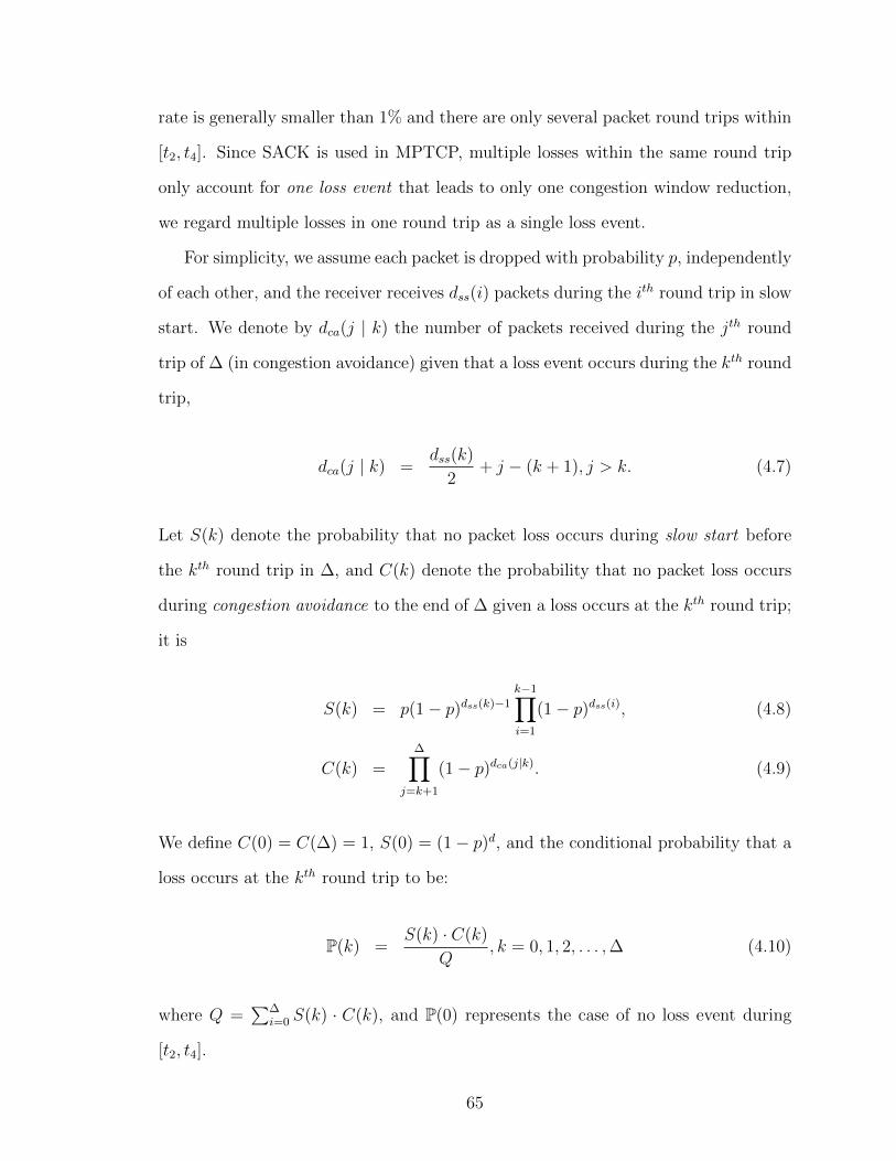
rate is generally smaller than 1% and there are only several packet round trips within

[t2, t4]. Since SACK is used in MPTCP, multiple losses within the same round trip

only account for one loss event that leads to only one congestion window reduction,

we regard multiple losses in one round trip as a single loss event.

For simplicity, we assume each packet is dropped with probability p, independently

of each other, and the receiver receives dss(i) packets during the ith round trip in slow

start. We denote by dca(j | k) the number of packets received during the jth round

trip of ∆ (in congestion avoidance) given that a loss event occurs during the kth round

trip,

dca(j | k) =dss(k)

2+ j − (k + 1), j > k. (4.7)

Let S(k) denote the probability that no packet loss occurs during slow start before

the kth round trip in ∆, and C(k) denote the probability that no packet loss occurs

during congestion avoidance to the end of ∆ given a loss occurs at the kth round trip;

it is

S(k) = p(1− p)dss(k)−1

k−1∏i=1

(1− p)dss(i), (4.8)

C(k) =∆∏

j=k+1

(1− p)dca(j|k). (4.9)

We define C(0) = C(∆) = 1, S(0) = (1− p)d, and the conditional probability that a

loss occurs at the kth round trip to be:

P(k) =S(k) · C(k)

Q, k = 0, 1, 2, . . . ,∆ (4.10)

where Q =∑∆

i=0 S(k) · C(k), and P(0) represents the case of no loss event during

[t2, t4].

65

Denote by d(k) the number of total packets received by the end of [t2, t4] from the

first flow given a loss occurs at the kth round trip; we have:

d(k) =

∆∑i=1

dss(i) , if k = 0.

k∑i=1

dss(i)− 1 +∆∑

j=k+1

dca(j | k) , otherwise.

(4.11)

The expected number of packets received from the first flow before the delayed second

flow starts is

E[ received packets ] =∆∑k=0

P(k) · d(k). (4.12)

Throughout our experiments, Iw = 10 and b = 2, we measure the average WiFi loss

rate (p = 0.009) and the RTT ratio from each of the 2-flow MPTCP connections

with all cellular carriers. The expected number of packets received before the delayed

second flow starts is depicted as the solid line in Fig. 4.2. By fitting the empirical

averages of different γ to the expected values derived from our model, the regression

statistics show R2 = 0.8758, indicating a good fit to our model.

When WiFi’s loss rate is about 0.9%, before the delayed cellular flow starts, a

user can receive an average number of 67, 88, and 130 packets respectively from

the WiFi flow while the cellular flow is AT&T, Verizon, and Sprint with a median

RTT ratio γ of 3.9, 4.4, and 6.0, respectively. That is, for small file transfers, the

MPTCP’s delayed startup of additional cellular flows results in the low utilization of

these flows. In the following section, we focus on larger file transfers and investigate

MPTCP performance issues affected by cellular network’s over-buffering.

4.4 MPTCP Performance Evaluation with Cellular Networks

We investigate the fact that cellular networks exhibit inflated and varying RTTs,

also known as bufferbloat. As we have observed such phenomenon in our measure-

66

2 3 4 5 6 7

5010

015

020

025

0

γ = RTT2 RTT1

rece

ived

pac

kets

AT&T 4GVerizon 4GSprint 3G

no loss no loss or one loss

Figure 4.2. Approximation of the expected number of received packets from thefirst flow as a function of RTT ratio. Samples are MPTCP measurements for differentcarriers of file sizes 1MB to 32MB.

ments, we analyze and model this phenomenon and evaluate the impact of this in

terms of RTTs and loss rates. Last, we show that severe bufferbloat can lead to low

flow utilization and eventually degrade MPTCP performance.

4.4.1 Understanding Bufferbloat and RTT Variation

The phenomenon of large and varying RTTs in cellular networks has been recently

observed and termed bufferbloat [33], which occurs due to the existence of large buffers

in the networks. Results from our earlier measurement study [20] are consistent with

previous studies by Allman [9] and Jiang et al. [52], which show that bufferbloat is

less prominent in most wired/WiFi networks (i.e., public/home WiFi networks), and

can be severe in 3G/4G cellular networks. However, in addition to the severe RTT

inflation of the cellular networks, we also observe that cellular networks exhibit very

low loss rates. Our measurements of downloads of file sizes 8 KB to 32 MB among all

the cellular carriers indicate loss rates less than 0.03%, which are much smaller than

those of WiFi, which are approximately 0.9%.

67

0

100

200

400

600

800

1000

1200

1400

8K 16K 32K 64K 128K 256K 512K 1M 2M 4M 8M 16M 32MFile Size (Byte)

RT

T (

ms)

isp

Sprint 3GVerizon 4GAT&T 4GWiFi

Figure 4.3. Average connection RTT as a function of file sizes for different carriers(mean ± standard error).

Fig. 4.3 presents the measurement results of average connection RTT as a function

of file size. Throughout the measurements, WiFi exhibits a stable average connection

RTT of approximately 30 ms while AT&T LTE exhibits an average RTT that ranges

from 60 ms to 180 ms as file size increases. Sprint 3G exhibits the greatest RTT

variability among all the carriers, with averages ranging from 160 ms to 1.2 second.

Verizon LTE, although using the same 4G technology as AT&T LTE, also exhibits

high variability in its RTTs, and the averages range from 60 ms to 900 ms as the

transferred file size increases. That is, γ can quickly rise from 2 to 40, and in some

cases up to 80.

In the following we seek to understand how RTT inflation occurs due to network

over-buffering. Let us denote by µ the network bandwidth, by τ the minimum packet

RTT, and the minimum bandwidth-delay product (BDP) by µτ . We denote the size

of network buffer by B, and the network storage capacity by F , which is the maximum

number of in-flight packets that can be stored in the network, including one BDP and

the size of the network buffer; hence F = dB + µτe. Although early works suggested

network buffer sizes are much smaller than the average BDP [11, 14], recent studies

68

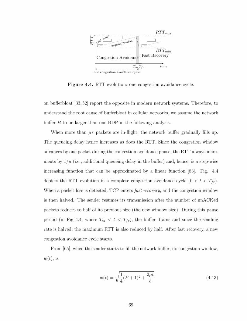
time

RTT

Congestion Avoidance

RTTmax

RTTmin

real va

lue

approximation

Tca Tfr

Fast Recovery

one congestion avoidance cycle

Figure 4.4. RTT evolution: one congestion avoidance cycle.

on bufferbloat [33,52] report the opposite in modern network systems. Therefore, to

understand the root cause of bufferbloat in cellular networks, we assume the network

buffer B to be larger than one BDP in the following analysis.

When more than µτ packets are in-flight, the network buffer gradually fills up.

The queueing delay hence increases as does the RTT. Since the congestion window

advances by one packet during the congestion avoidance phase, the RTT always incre-

ments by 1/µ (i.e., additional queueing delay in the buffer) and, hence, is a step-wise

increasing function that can be approximated by a linear function [83]. Fig. 4.4

depicts the RTT evolution in a complete congestion avoidance cycle (0 < t < Tfr).

When a packet loss is detected, TCP enters fast recovery, and the congestion window

is then halved. The sender resumes its transmission after the number of unACKed

packets reduces to half of its previous size (the new window size). During this pause

period (in Fig 4.4, where Tca < t < Tfr), the buffer drains and since the sending

rate is halved, the maximum RTT is also reduced by half. After fast recovery, a new

congestion avoidance cycle starts.

From [65], when the sender starts to fill the network buffer, its congestion window,

w(t), is

w(t) =

√1

4(F + 1)2 +

2µt

b(4.13)

69

where b is the delayed ACK parameter (i.e., an ACK is generated at the reception

of every b packets). When w(t) reaches the network storage capacity F at time Tca

(the end of the congestion avoidance phase), by solving Eq. (4.13) for w(Tca) = F ,

we obtain Tca = 3b8µ

(F + 1)2.

That is, during one congestion avoidance cycle, µTca packets are transmitted,

and then one additional window of packets is sent before the lost packet is detected.

Therefore, the number of packets sent during a congestion avoidance cycle is N ≈

d3b8

(F + 1)2 +F e (excluding the retransmitted packet). If we assume packets are only

dropped due to the filled network buffer, then within one congestion avoidance cycle,

the loss rate is 1/N .

Fig. 4.5 depicts the network loss rate, 1/N , as a function of network storage

capacity F . Given a network bandwidth µ = 10 Mbps and τ = 15 ms, with the TCP

delayed ACK parameter b = 2, the minimum BDP is roughly 12 packets. By setting

a buffer size equal to the minimum BDP (B = µτ), the loss rate drops from 0.7%

to 0.2%. When the buffer size increases 8-fold, the loss rate drops to 0.01%. Hence,

if we assume the minimum BDP does not change during each cycle, and packets are

dropped only due to the filled network buffer, increasing the buffer size reduces the

loss rate dramatically.

Since the network over-buffering issue has been recently reported by [33] and is

termed as bufferbloat, our analyses above shed light on how bufferbloat can result in

extremely small loss rates while exhibiting the large RTT variations observed in our

measurements. When flow RTTs are small and stable, ACKs return to the sender

quickly and the RTT estimates are precise. However, when one of the MPTCP flows

exhibits small and stable RTTs while the other experiences severe RTT inflation

without packet losses, the joint congestion controller can be misguided by TCP’s

congestion inference from packet losses, and lose its ability to quickly balance con-

70

F = B + µ τ (#packets)

loss

rat

e (%

) in

log

sacl

e0.

005

0.01

0.05

0.1

0.5

1

10 50 100 150 200 250

Figure 4.5. Network loss rate as a function of network storage F .

gestion across the flows. In the following, we investigate how inflated cellular RTTs

can affect MPTCP performance.

4.4.2 Idle Spins of the Joint Congestion Controller

The coupled congestion controller increases the congestion window of flow i upon

reception of each ACK with wi = wi + min(α/w, 1/wi), where w =∑

iwi. Since this

controller does not couple the decrease phase, it relies on α to respond to changes in

flow windows and RTTs, and α is defined in [77] as:

α =max{ wi

R2i}

(∑

iwiRi

)2· w (4.14)

As α is updated whenever there is a packet drop or once per RTT rather than once

per ACK to reduce computational cost [77], this results in slow responsiveness of α to

network dynamics. Moreover, since ACKs are used at the sender for RTT estimation

and TCP uses delayed ACK, when the network is over-buffered, the sender fails to

estimate the RTT in a timely manner. Also, the RTT values used in Eq. (4.14) are

smoothed values (SRTT) with the consequence that they lag behind the true RTTs

71

RTT ratio: γ

flow

incr

emen

t effi

cien

cy

2 3 4 5 6 7 8 9 10

0.1

0.2

0.3

0.4

0.5

0.6

0.7

β = 2β = 3β = 4

Figure 4.6. MPTCP flow increment efficiency as a function of γ.

when they are rapidly increasing. As a result, the coupled congestion controller

underestimates α, and hence the MPTCP increase rate.

For a simple 2-flow MPTCP with congestion window ratio β = w2/w1 and RTT

ratio γ = R2/R1, if we assume in Eq. (4.14) that the numerator has w1/R21 ≥ w2/R

22

(i.e., flow 1 is currently the better flow [89]), then the MPTCP window increase rate

can be rewritten as

α

w=

w1

R21

(w1

R1+ βw1

γR1)2

=1

(1 + β/γ)2· 1

w1

. (4.15)

Upon reception of each ACK, flow 1 increases w1 by 1(1+β/γ)2

· 1w1

. We define flow

increment efficiency as the ratio of a flow’s increase rate when running MPTCP to

that of running single-path TCP (i.e., 1/(1+β/γ)2). Fig. 4.6 shows flow 1’s increment

efficiency as a function of RTT ratio γ for different window ratios β.

Since cellular networks exhibit loss rates typically smaller than 0.03% [20], the

cellular flow’s window is often larger than that of the WiFi flow. For a 2-flow MPTCP

connection (e.g., WiFi the first and cellular the second) with β = 2, when the cellular

RTT inflates, γ can ramp up quickly from 2 to 8 as more packets are in-flight (as

72

shown in Fig. 4.3). As depicted in Fig. 4.6, if we assume the window ratio β remains

fixed at 2, and the inflated RTTs can be correctly estimated during the cellular RTT

inflation period while γ increases from 2 to 8, the WiFi flow’s increment efficiency

should increase from 0.25 to 0.65. However, due to the slow responsiveness of α and

the cellular flow’s lagged RTT estimates, the WiFi flow’s increment efficiency remains

at 0.25 for at least one RTT. Thus, the WiFi flow’s increase rate is underestimated

by 61% during this cellular RTT inflation period.

This issue becomes more critical when the cellular flow, henceforth referred to

as flow 2, fails to receive new ACKs from the client even after the sender performs

fast retransmit (within R2), and eventually its timeout timer expires after one re-

transmission timeout (RTO)3. The idle period during which flow 2 does not send any

packets, has length Tidle ≈ RTO−R2, and the period can be longer when bufferbloat

is more prominent. During Tidle, the aggregate window, w, still remains large as flow

2’s congestion window, w2, will only be reset to two after the timeout event. The

WiFi flow’s (flow 1) increase rate, α/w, is therefore very small due to this large w.

Moreover, during Tidle, packets are only delivered over flow 1. Flow 1’s bandwidth, as

we have observed, is severely underestimated and its increase rate should have been

raised to 1/w1 as that of a single-path TCP.

Ideally when an MPTCP connection includes different flows characterized by di-

verse but stable RTTs, α can be set to respond network changes quickly and the cou-

pled congestion controller should achieve MPTCP’s desired throughput. However,

since cellular networks exhibit bufferbloat, which in turn results in large congestion

windows and unstable RTTs, these properties eventually lead to MPTCP performance

issues.

3RTO = SRTT + max{G, 4×RTTV AR}, where RTTV AR is the RTT variance, and the initialvalue of RTO is 1 sec [75]. Note that G is the clock granularity set to 0.2 sec in modern Linuxsystems.

73

4.4.3 Flow Starvation and TCP Idle Restart

MPTCP maintains a connection-level shared send queue for all the packets sched-

uled to be sent, while each flow manages its own subflow-level send buffer. When a

flow has available space in its congestion window, the MPTCP packet scheduler clones

the first segment at the head of the shared send queue into the flow send buffer4.

When all previously sent packets over a particular flow are ACKed (subflow-level

ACK), the data in the subflow-level send buffer can be removed. The original segment,

however, remains in the connection-level shared send queue until all older packets are

correctly received and ACKed (connection-level ACK) via the other flows. That

is, when a packet in the shared send queue is ACKed at the subflow level and the

connection level, it is still retained in the connection-level send queue while any older

packets with smaller connection-level sequence numbers have not yet been reported

as received. Once those older packets are received and ACKed, the connection-level

ACKed packets are dequeued, and new packets from the application are appended to

the tail of the connection-level send queue.

When one of the MPTCP flows suffers severe bufferbloat and the transmission

latency quickly increases, packets may take unexpectedly longer to reach the receiver.

Suppose the connection-level send queue has capacity M , and the first i packets are

currently scheduled on the cellular flow, experiencing severe bufferbloat, while the

i+ 1th to jth packets are scheduled to the WiFi flow. Since WiFi has a much smaller

RTT than cellular, the WiFi flow packets are quickly ACKed, and removed from

their flow send buffer. The WiFi flow then has space in its congestion window and

requests more packets from the connection-level send buffer (the j+1th to M th). Note

that at this point in time, packets traversing cellular are experiencing high latency

due to bufferbloat, and the first i packets are still en-route while the WiFi flow has

4This is true when no packet is in the connection-level retranmission queue.

74

successfully received ACKs for the i+ 1th to M th packets. Up until this point, those

M − i packets sent over WiFi are ACKed at the subflow level, and hence no data is

retained in the WiFi flow send buffer. On the other hand, their original copies still

remain in the connection-level send buffer, waiting for the first i packets sent over

cellular to reach the receiver. Before the oldest i packets in the queue are correctly

received and ACKed, the connection-level send queue fills up (the first i packets over

the cellular flow, and M − i ACKed packets waiting for the oldest i packets to be

ACKed).

This leads to flow starvation. The WiFi flow has now removed all the ACKed

data from its send buffer (subflow-level ACKed), and requested new packets from

the shared send queue. The shared send queue, on the other hand, has no available

packets to allocate to the WiFi flow. Moreover, it can not request any new packets

from the application layer, as currently the shared send queue is full. This dilemma

ends only when the oldest packets in the queue are correctly received and ACKed, the

application places new data in the connection-level send queue, and the WiFi flow

resumes.

The consequence of an idle MPTCP flow has far more impact than above. When

the WiFi flow’s idle period is longer than the current estimated flow retranmission

timeout (RTO) with window size w1, the TCP’s congestion window validation mech-

anism [39] is triggered and calculates a restart window, wr = min(w1, Iw), for the idle

WiFi flow. For each RTO event, w1 is halved until wr is reached5. After the WiFi

flow resumes and its window is reset to a new value, it is then forced to re-probe the

network with slow start.

Fig. 4.7 illustrates a time series of the WiFi flow’s congestion window and the

cellular flow’s RTT. Note that the cellular flow here suffers severe bufferbloat with

5Details please refer to the procedure tcp cwnd restart() in tcp output.c in the Linux kernel.

75

periodic RTT inflation as illustrated Fig. 4.4. At the beginning of the connection,

the cellular RTT inflates quickly from 80 ms to 800 ms, and hence produces the WiFi

flow’s first idle period soon after it enters congestion avoidance. The WiFi flow’s

congestion window is halved before the next slow start because it experiences an idle

period of one RTO. Note that this behavior is not due to loss events, as the congestion

window is often reset to wr rather than two as in a timeout event.

For the subsequent idle restarts in Fig. 4.7, WiFi’s congestion window is often

reset to Iw (i.e., the initial window of 10 packets). This phenomenon is very prominent

during time interval 20 to 32 seconds, where the cellular RTTs inflate dramatically

up to 3.5 seconds, and the WiFi idle period is much longer than its current RTO. The

phenomenon of RTT inflation is less pronounced after 35 seconds when the RTT drops

from 2 sec to 400 ms. After this point in time, the receiver receives packets from the

cellular flow more quickly, and the corresponding ACKs to those packets arrive at the

sender in a timely fashion without blocking the shared send queue. Hence, the WiFi

flow successfully completes slow start and enter congestion avoidance. During these

idle periods, not only does the WiFi flow starve, but the cellular flow exhibits a low

increment efficiency. This occurs for the same reason described in Sec. 4.4.2 when

one of the flows experiences a long idle period, the coupled controller underestimates

the increase rate and eventually degrade MPTCP’s performance.

To avoid unnecessary performance degradation due to bufferbloat, we propose

to disable the default idle restart functionality [39] when using MPTCP with cel-

lular. The benefit of doing so is two-fold. First, allowing an idle MPTCP flow to

quickly restore its original congestion window reduces network resource waste and

saves download time by not having to probe for the network capacity again. Second,

as the coupled controller couples all flows at the increase phase, each flow’s increase

rate is much slower than its single-path counterpart. Therefore, after an idle restart,

76

0 10 20 30 40

020

4060

80

time (sec)

CW

ND

(pa

cket

s)

050

010

0015

0020

0025

0030

0035

00

RT

T (

ms)

WiFi CWNDinitial CWNDRTT (cellular)

Figure 4.7. Severe bufferbloat: periodic RTT inflation of the cellular flow results inidle restarts of the WiFi flow.

it takes much longer for the restarted flow to reach the same sending rate before the

restart event.

To showcase how our proposed approach can effectively mitigate the impact of

flow starvation, Fig. 4.8 illustrates the results of MPTCP download times when TCP

idle restart (RST) is enabled/disabled. Moreover, as the penalizing scheme proposed

in [80] aims to optimize receive memory usage by reducing the window size of flows

that contribute too many out-of-order packets, we also show the results of MPTCP

with (w/ penl.) and without penalization (w/o penl.). Note that the MPTCP receive

buffer is set to the default maximum size of 6 MB, which is much larger than the

targeted scenario in [80]. We do not disable TCP auto-tuning as proposed in [74] as

our goal is to understand bufferbloat’s impact on MPTCP shared send buffer rather

than the efficiency of utilizing the receive buffer at the beginning of each connection.

We chose one cellular carrier that exhibits prominent bufferbloat during the day

and performed file downloads of 16 MB files with 2-flow MPTCP connections. For

each configuration, we performed 40 rounds of measurements and randomized the

order of the configurations to reduce possible correlations during our measurements.

77

no RST (w/ penl.)

RST (w/ penl.)

no RST (w/o penl.)

RST (w/o penl.)

16 MB

10 15 20Download Time (sec)

Figure 4.8. Download time comparison: MPTCP with idle restart (RST) and pe-nalization (penl.) enabled/disabled.

When the cellular flow experiences bufferbloat and idle restarts occur frequently, we

observe that MPTCP suffers severe performance degradation. The penalizing scheme

helps in this case by throttling the cellular flow’s sending rate and hence mitigates

bufferbloat. Furthermore, it delays the occurrence of the idle restarts and provides

an opportunity for those connection-level ACKs of the late received packets sent over

cellular to arrive at the sender and unblock the shared send buffer.

When the TCP idle restart is disabled, the download time (both mean and vari-

ance) reduces for both vanilla MPTCP (no RST w/o penl.) and the MPTCP with

penalization (no RST w/ penl.). We show that, when bufferbloat is evident, by dis-

abling the TCP idle restart, on average MPTCP download time decreases by 30%

(no RST w/ penl.).

4.5 Related Work

To the best of our knowledge, this is the first work that models the impact of

MPTCP’s flow delayed startup to understand when a user can start to leverage the

additional flows. It is also the first work that investigates the impact of bufferbloat

78

on MPTCP performance. Since the root cause of MPTCP performance problems of

flow starvation and idle restart is bufferbloat in the cellular networks, if cellular op-

erators can size their router buffers properly as suggested in [11, 14], the bufferbloat

issues can be mitigated. The associated MPTCP performance issues can hence be

resolved. Several works have recently aimed to tackle this issue based on existing

infrastructure. Jiang et al. [52] proposed a receiver-based rate limiting approach to

mitigate the RTT inflation by tracking down the RTT evolution. Nichols and Jacob-

son proposed a scheduling algorithm, CoDel [72], to control network delay through

managing router buffers. These approaches require additional changes and manage-

ment at the receivers and at the buffers within the network, and might directly affect

the performance of MPTCP from different perspectives. If MPTCP can wisely select

available paths and flows to leverage [59] without being hampered by bufferbloat, and

the joint congestion controller can be more responsive to the rapid variation of RTTs,

the benefits of MPTCP will be more pronounced. As these require further study and

more careful examination in the networks, we leave these as future works.

4.6 Conclusion and Discussion

In this chapter, we study the performance of a simple scenario of 2-flow MPTCP

with WiFi and cellular networks. We show that for small downloads, the current

MPTCP’s delayed startup of additional flows limits MPTCP’s performance. Based on

the RTT ratio of the WiFi and cellular networks, we demonstrate that the additional

flows can be underutilized for small file transfers by modeling the number of packets

received before the second flow starts. Second, as we have observed bufferbloat in the

cellular networks, we investigate the root cause of large and varying cellular RTTs

by modeling and analyzing bufferbloat. Furthermore, we show how MPTCP might

suffer from cellular bufferbloat when coupling with another WiFi flow for large file

transfers. Last, we show how flow starvation occurs when bufferbloat is prominent and

79

can eventually harm MPTCP’s performance. By disabling the TCP idle restart for

congestion window validation, we show that this is an efficient approach to mitigate

the MPTCP performance degradation.

So far, we understand how well multi-path TCP performs in the wild in terms of

different flow sizes, and how it can leverage both cellular and WiFi paths to provide

robust mobile data transport. Moreover, MPTCP congestion controller performs dy-

namic load balancing and offloads traffic from congested paths (or overloaded APs)

to those paths of better link quality. On the other hand, MPTCP only works well

on traditional end-to-end, server- client model where either or both ends might be

multi-homed. With tremendous traffic growth from mobile devices, when the targeted

server is overloaded or paths to this server have been fully utilized, mobile clients can

still suffer poor performance and bad quality of service. The emergence of content

delivery networks (CDNs), or telco CDNs (CDNs owned by telecommunication ser-

vice providers), popular content or videos nowadays have replicas stored at multiple

locations (at different servers or data centers) accessible to users. As mobile users

path quality can change over time, we seek to enhance current MPTCP implemen-

tation to allow a user to fetch content from multiple sources. With a good selection

of available paths of dynamic link qualities, this approach can shorten the download

latency and provide better quality of service.

80

CHAPTER 5

MSPLAYER: MULTI-SOURCE AND MULTI-PATHVIDEO STREAMING

With the high demand for online video streaming, video content providers are

offering better technology to satisfy customers’ desires for streaming high quality

videos. However, streaming video to a user nowadays still encounters the follow-

ing challenges. First, people from time to time experience insufficient bandwidth

when streaming videos. Research has shown that viewers are not patient enough

to wait if the start-up delay is longer than a few seconds [64]. In addition, video

quality has a huge impact on user engagement. Users tend to drop videos if they

frequently encounter videos that stop, pause, freeze or experience quality changes

during the playout [24]. Also, connections to a particular network can break down

temporarily due to mobility and re-establishing a connection introduces additional

delays. Last, as network bandwidth is highly variable, the commercial video players

have experimented with video rate adaption, which in turn results in unstable perfor-

mance such as variable video quality, unfairness to other players, and low bandwidth

utilization [6, 7, 49,53,70].

As mobile devices are now equipped with multiple wireless interfaces connected

to different networks (WiFi or cellular 3G/4G), one possible solution to the above

challenges is to use multi-path TCP (MPTCP) [31]. However, since MPTCP requires

kernel modifications at both the client and server sides [80], and many network op-

erators do not allow MPTCP traffic to pass their middleboxes [42, 44], MPTCP has

been slow to deploy globally. Furthermore, although MPTCP provides a means for

81

balancing loads over different paths to a single server, it does not utilize source di-

versity present in networks in order to facilitate content delivery. Therefore, there is

the potential to develop a solution to stream high quality videos to end users with-

out overloading the video servers and network resources. Thus, we ask the following

question: Is it possible to leverage both path diversity and source diversity to provide

robust video delivery and to reduce video start-up latency?

In this chapter, we take a first step to answering this question. We show that one

can utilize both of the available WiFi and 4G interfaces simultaneously to aggregate

bandwidth for higher quality video streaming. The video streaming solution does not

require modifications in the kernel stacks and is not hindered by network middleboxes.

We instantiate these designs in our YouTube player, MSPlayer. By investigating the

YouTube service architecture and its streaming mechanisms, we further demonstrate

how to simultaneously leverage the existence of multiple video sources in different

networks. We then experimentally evaluate the performance of different MSPlayer

schedulers as well as the performance of MSPlayer through the YouTube service.

The remainder of this chapter is organized as follows: Sec. 5.1 introduces the de-

sign principles of MSPlayer. We overview the architecture of MSPlayer in Sec. 5.2.

Implementation details of MSPlayer are presented in Sec. 5.3 and we evaluate MSPlayer’s

performance in our testbed and over YouTube infrastructure in Sec. 5.4 and 5.5. We

discuss future work and conclude this chapter in Sec. 5.6. The research described was

published in [23].

82

5.1 Design Principles

In this chapter, we present MSPlayer, a client-based approach for video streaming

that requires no changes in either the server or the client’s kernel stacks. It leverages

diversity in the network and performs load balancing at the client side. MSPlayer

also supports user mobility and provides robust data transport. In order to be fair

to other TCP users, MSPlayer limits the number of paths to two (one over WiFi and

one over 3G/4G) and leverages HTTP range requests to stream videos. It has the

following design features.

Just-in-time with High Quality: Since viewers often prematurely stop watching

videos [28,64], streaming the entire video to a viewer at once can waste bandwidth and

network resources. This, along with the rise of adaptive streaming over HTTP [85],

has drawn attention to just-in-time video delivery, which has been exploited by most

large scale video streaming services such as YouTube, Netflix, and Hulu. A video

is partitioned into many small file segments called video chunks. The video server

maintains multiple profiles of the same video for different bitrates and video quality

levels. Clients then periodically request video chunks and adapt video bitrates.

Just-in-time video delivery avoids a waste of resources if a user drops the video

during its playback. Dynamically adapting video bitrates, however, results in perfor-

mance problems such as low link utilization [6], unfairness to other TCP users [6,49],

and unstable video quality [7, 70]. In our design, we share the just-in-time concept

for video delivery. However, we do not investigate rate adaption and instead focus on

how to stream videos to users with a fixed bitrate by exploiting network diversity.

Robust Data Transport: When a mobile user streams a video, his connection

(mostly WiFi) can break and the downloaded video will thus be abandoned. In order

to resume the video, the user then needs to switch to another available interface con-

83

nected to another network, establish a new TCP connection, and move/skip to the

break point. In the worst case, one has to wait until reaching the next WiFi hotspot

and repeat the entire process mentioned above.

One possible solution is to use Multi-Path TCP (MPTCP) [31], which has been

standardized by the IETF, aimed at providing robust data transport. However,

MPTCP still faces several deployment challenges: First, MPTCP requires kernel

modifications at both the server and client [31]. Second, it relies on the TCP op-

tion field to exchange path and interface information. In the latter case, research

has shown that MPTCP suffers significantly from network middleboxes as they very

often strip away unknown options [42, 44], forcing MPTCP connections to fall back

to legacy single-path TCP. In our measurements, two out of three major US cellu-

lar carriers do not allow MPTCP traffic to pass through the default HTTP 80 port,

which is a potential problem for video streaming to popular sites such as YouTube or

Netflix.

We design a client-based multi-path solution to provide robust data transport for

high quality video streaming. Furthermore, each path runs legacy TCP and is there-

fore guaranteed to successfully pass network middleboxes.

Content Source Diversity: Current MPTCP [31] and other similar approaches

such as [16], only allow flows or paths to be established between a client and a sin-

gle server. If the current YouTube infrastructure were to support MPTCP, users

streaming videos from one server with high aggregate bandwidth through multiple

paths could quickly incur server demand surges. This high demand, particularly for

high quality videos, can overload the server and congest shared bottleneck links. The

outcome of this can directly or implicitly affect other viewers’ experience.

84

As popular content is now replicated at multiple locations or data centers, content

delivery networks (CDNs) are responsible for handling video replicas and delivering

videos across different data centers for large scale video streaming services such as

YouTube, Netflix, and Hulu [2, 3]. As part of our design is to provide robustness,

MSPlayer, at the initial phase, collects a list of YouTube servers’ addresses in each

network exploited. If a server in a network fails or is overloaded, MSPlayer switches

to another server in that network and resumes video streaming. Other proposals,

such as [37], aim to emulate the use of multiple paths in a controlled environment by

setting up multiple connections to the servers connected by a switch with only one

single interface. Although this approach can potentially distribute the load among

the connected servers, having multiple connections over one interface could quickly

saturate the bottleneck link.

As wireless interfaces are associated with different networks, MSPlayer requests

partial content from video servers in all networks simultaneously to avoid overwhelm-

ing particular video servers and to balance the load across the servers. In this work,

we use Google’s public DNS service to resolve the IP addresses of YouTube servers.

Chunk Scheduler: MSPlayer relies on HTTP range requests to retrieve video

chunks over different paths. As making a range request incurs additional overhead

(packets start to arrive one RTT after the request is sent) and different paths usu-

ally exhibit diverse latencies [20], efficient scheduling of chunks over different paths

is challenging. Therefore, it is desirable to have a good scheduler that estimates path

quality over time and efficiently assigns chunks to each path.

To satisfy just-in-time video delivery, the scheduler pauses chunk retrieval when

the playout buffer is full and resumes chunk retrieval when the amount of buffered

video falls below a certain level (that is referred to as periodic downloading or

ON/OFF cycles [81]). To reduce memory usage of out-of-order chunks from dif-

85

12 3 4 5 6

9

2

78

t0

JSON3WHS FIN

1kRTT 1kRTT 1kRTTk+kΔ2k 1kRTT 2kRTT 1kRTT

Δ2server

client

ClientkHello

3 ServerkHello

4 Certificate

5 ServerkHellokDone,kServerkKeykExchange

7 NewkSessionkTicket

ClientkKeykExchange

JSON data

HTTP request

t1 t2 t3 t4 t5 t6

Δ1

6

Δ1

Figure 5.1. HTTPS connection to YouTube web server: retrieving JSON objects ofvideo information.

ferent paths, the MSPlayer scheduler attempts to complete the transfer of a chunk

over each path at the same time, and allows at most one out-of-order chunk to be

stored.

5.2 MSPlayer Overview

We now overview the MSPlayer architecture. We first describe how YouTube

video streaming works and the just-in-time video delivery, followed by descriptions of

the MSPlayer’s design components: multi-source, multi-path, and chuck scheduler.

5.2.1 YouTube Video Streaming

Users either go to the YouTube website and choose a video to watch, or click

on an URL of the following form http://www.youtube.com/watch?v=qjT4T2gU9sM

on a web page. Users then watch the video through their browsers using a built-in

Adobe Flash player [5]. Each YouTube video is identified by an 11-literal video ID

after watch?v= in the URL [3].

With this URL, the video player (e.g., Adobe Flash) first performs a DNS lookup

to resolve the IP address of the domain name www.youtube.com and the user’s video

request is then directed to one of YouTube’s web proxy servers. The YouTube web

86

proxy server processes the request and returns the related video information and a

new URL to the user in JavaScript Object Notation (JSON) format, indicating where

the associated and available YouTube video servers are. The player then establishes

another connection to one of the dedicated video servers and starts to stream the

YouTube video using HTTP range requests.

The streaming process starts with a pre-buffering phase followed by a periodic

re-buffering phase [81]. The pre-buffering phase takes place at the beginning of the

streaming and aims at retrieving enough video data into the playout buffer for the

initial video playout. After the player consumes the video content for a while and the

amount of video in the playout buffer falls below a certain level, the player enters the

re-buffering phase, and make new requests periodically to refill the playout buffer.

This periodic re-buffering repeats until the video is completely watched or dropped.

5.2.2 Multi-Source and Multi-Path

Before describing our scheme with multiple sources and multiple paths, we first

describe how each path establishes a connection to the YouTube web proxy server and

the associated video server. Fig. 5.1 illustrates a flow diagram when a user contacts

YouTube’s web proxy server to retrieve video information. The connection starts with

a TCP 3-way handshake (3WHS). Afterwards, the client initiates a secure connection

handshake message at time t1. It takes the server times ∆1 and ∆2 to verify the key

and complete the key exchange process. The first HTTP request is made at time t3,

and the first JSON packet from the web proxy server arrives at t4. Note that these

JSON packets are delivered within two round trips (slightly less than 20 packets)1,

and the secure connection ends at t5 followed by a TCP FIN.

1As of July 2014, YouTube has applied algorithms to encode copyrighted video signatures. Sincethese signatures are needed to contact the video servers, for copyrighted videos, an additional oper-ation is required to fetch the video web page containing a decoder to decipher the video signature.

87

If we denote by R1 and R2 the RTTs of the first and the second paths, and by

θ = R2/R1 the RTT ratio (assuming R1 ≤ R2, i.e., the first path is a fast path), it

takes time ηi = 4Ri + ∆1 + ∆2 to establish a secure HTTP connection over path i,

and time ψi = 6Ri+ ∆1 + ∆2 to receive complete video information before contacting

the video server. If the YouTube’s web proxy server is close to the video server,

and both servers have similar capabilities for key verification, it takes approximately

πi ≈ ψi + ηi seconds for path i to receive the first video packet from the video server.

When fetching video content, MSPlayer contacts a video server over one path

as soon as the IP address of the video server associated with that path is decoded,

and does not wait for the decoding process over other paths to finish. Chunks are

scheduled over the first path before the second path becomes available. Therefore,

before the second path starts to retrieve video packets from its associated video server,

the first path will have received video packets for a duration of π2−π1 ≈ 10·(R2−R1) =

10 · (θ − 1)R1.

In MSPlayer, the processes of fetching video chunks over each path are executed

by independent threads under the management of the chunk scheduler (described in

the next section).

5.2.3 Chunk Scheduler

In order to reduce out-of-order delay for video streaming, and to reduce memory

needed to store out-of-order chunks, our goal is to schedule chunks (of different sizes)

over both paths so that chunk transfers complete at roughly the same time.

To optimize video streaming performance with MSPlayer, chunk size selection for

each path is critical and should be adapted over time in response to network dynamics.

A previous measurement study shows that YouTube players, such as Adobe Flash

or HTML5, use 64 KB and 256 KB as their default chunk sizes, while Netflix player

(silverlight) uses larger chunk sizes that range from 2 MB to 4 MB [81]. Since different

88

mobile devices have pre-buffering periods of different lengths (ranging from 20 seconds

to 1 minute) [80], we also investigate the performance of different schedulers when

applying different chunk sizes and pre-buffering periods.

We denote by Si(t) the chunk size of path i at time t, by B the base chunk size,

and by Ti the time required to download chunk Si(t). The estimated throughput to

download Si(t) is denoted by wi(t) = Si(t)/Ti.

We first showcase a baseline scheduler called Ratio and then propose two differ-

ent chunk size schedulers that adjust chunk sizes according to network bandwidth

changes, namely the exponential weighted moving average (EWMA) and Harmonic.

MSPlayer’s chunk size selection should adapt to path quality variations over time,

and the bandwidth estimator of MSPlayer thus plays a critical role in the chunk

size selection process. In this chapter, we label the chunk scheduler according to the

bandwidth estimator used. We compare and evaluate the performance of these three

schedulers in our testbed.

Baseline Scheduler: Suppose wi(t) ≤ w1−i(t), the baseline Ratio scheduler assigns

a fixed chunk size to the path with lower throughput such that Si(t + 1) = B and

adjusts the chunk size of the path with higher throughput based on throughput ratio

(i.e., S1−i(t+1) = w1−i(t)/wi(t)·B where i = 0, 1 labels the first and the second path).

Dynamic Chunk Adjustment Scheduler: When path bandwidth estimates are

available, the chunk size of each path is adjusted according to Algorithm 1. We de-

note by δ the throughput variation parameter. If the current bandwidth measurement

of the slow path is (1 + δ) times larger than the estimated value, the chunk size is

doubled. Similarly, if the current value is (1 − δ) times smaller than the estimated

value, the chunk size is halved. The chunk size of the fast path is adjusted based on

the throughput ratio.

89

Algorithm 1 Dynamic chunk size adjustment1: procedure DCSA(i, w0, w1, wi, δ, B) . i = 0,12: if wi not available then3: Si ← B . initial chunk size4: else if wi < w1−i then . slow path5: if wi > (1 + δ)wi then6: Si ← 2 · Si7: else if wi < (1− δ)wi then8: Si ← max{dSi/2e, 16KB}9: else

10: Si unchanged11: end if12: else . fast path13: γ = dwi/w1−ie14: Si ← γ · S1−i15: end if16: return Si . final chunk size17: end procedure

Here we focus on two bandwidth estimators: exponential weighted moving average

(EWMA) and harmonic mean (Harmonic). The weighted moving average is defined

as:

wi(t+ 1) = α · wi(t) + (1− α) · wi(t). (5.1)

In this chapter we only report results for α = 0.9 (details see next section).

As network bandwidth can vary quickly, extreme measurement values can bias

our bandwidth estimation. Hence, we introduce another bandwidth estimator called

harmonic mean. The benefit to estimating path bandwidth by harmonic mean is that

it tends to mitigate the impact of large outliers due to network variations [53].

Given a series of bandwidth measurements, wi(t), where t =0, 1, 2, · · · , n − 1 and

wi(t) > 0, the harmonic mean is

wi(n) = n/n−1∑t=0

1

wi(t). (5.2)

The harmonic mean can be computed by maintaining all or a window of the most

recent measurements [53]. However, to reduce memory usage and computational

cost, one can compute the current harmonic mean without maintaining all previous

90

observations. Statistics from the past can be recovered simply by recording an ad-

ditional parameter, n, the total number of past measurements. The harmonic mean

can be updated with the most recent measurement of path i, wi(n), and the previous

harmonic mean wi(n). That is,

wi(n+ 1) =n+ 1∑nt=0

1wi(t)

=n+ 1

nwi(n)

+ 1wi(n+1)

. (5.3)

In the following sections, we present MSPlayer implementation details and evalu-

ate MSPlayer’s performance.

5.3 MSPlayer Implementation

In order to exploit both available wireless interfaces simultaneously, we pass addi-

tional interface information to the socket API to bind each interface to an IP address

and packets can thus be scheduled to a desired interface. Moreover, we configure

an independent routing table for each interface so that when a source IP address is

specified, instead of using the default interface and gateway, the desired interface and

gateway are used. Since video players can access YouTube videos through Google’s

Data APIs [36], MSPlayer is developed to leverage source and path diversity in the

network for YouTube video streaming by interacting with Google APIs.2

First, when the desired video object is chosen, the player contacts the web proxy

server with the URL containing the 11-literal video ID. The web proxy server then

authenticates the user (player type and/or the user account) with OAuth 2.0 and

verifies the video operations requested by the user [36]. When the requested opera-

tions are granted, the web proxy server resolves the user’s public IP address and check

to see which video server is suitable and available to this user based on YouTube’s

2As YouTube’s client libraries are mostly in web languages, MSPlayer, however is programmedin python rather than JavaScript or PHP.

91

server selection mechanism [4]. Afterwards, the web proxy server generates an access

token (valid for an hour) that matches the video server’s IP address as well as the

operations requested.

The web proxy server then encodes the token, together with the user’s public IP

address and the video’s information (i.e., available video formats and quality, title,

author, file size, video server domain names, . . . , etc) in JavaScript Object Notation

(JSON) format and returns these objects to the user through the requested interface.

MSPlayer then decodes the JSON objects received on each interface and synthesizes

a new URL (with the required information, video server address, and a valid token)

to contact the corresponding video server in the associated network. Video content

is then retrieved by making HTTP range requests to different video servers with

persistent connections through both interfaces. Note that YouTube has been grad-

ually replacing insecure HTTP connections with secure ones. To be compatible to

the current and future YouTube’s data service, we follow YouTube’s latest HTTPS

connection policy with both web proxy servers and video servers.

As part of the just-in-time video delivery principle, MSPlayer uses the following

streaming strategy similar to commercial YouTube players such as Adobe Flash player

or HTML5: a pre-buffering phase followed by a steady-state re-buffering phase [81].

MSPlayer leaves the pre-buffering phase when more than 40-second video data is

received. It then consumes the video data until the playout buffer contains less than

10-second video. MSPlayer resumes requesting chunks from both YouTube servers

and refills the playout buffer until 20 seconds of video data are retrieved.

5.4 Testbed Experimentation

We first evaluate the performance of each component of MSPlayer on a testbed

in a controlled environment that emulates YouTube’s video streaming mechanisms.

The final performance evaluation is carried out on the YouTube infrastructure and

92

service (see Sec. 5.5). Two types of servers are emulated in our testbed: web proxy

servers (responsible for authentication and video object information delivery) and

video servers. Both types of servers use the standard Linux 3.5 kernel with CUBIC

congestion control [34] coupled with Apache service. Each type of server is hosted in

two different UMass subnets for source diversity.

The client running MSPlayer is a Lenovo X220 laptop equipped with a built-

in 802.11 a/b/g/n WiFi interface connecting to a home WiFi network and an LTE

dongle connecting to one of the major US cellular carriers. Video requests are sent

over both interfaces simultaneously to two different YouTube video web proxy servers.

Upon receiving packets from the web server, MSPlayer decodes the associated JSON

objects (with a pre-loaded video server’s IP address in our testbed) and fetches video

chunks from the video servers. In our testbed, the videos are pre-downloaded in the

servers from YouTube with MP4 format of HD (720p) video quality and 44,100 Hz

audio quality.

5.4.1 Multi-Source and Multi-Path

Fig. 5.2 demonstrates the initial video pre-buffering download time using single-

path WiFi, single-path LTE, and MSPlayer for HD videos in our emulated testbed.

Note that a 40-sec pre-buffering period is presented here as this is YouTube servers’ de-

fault pre-buffering size for Flash videos [81]. The median download time of MSPlayer

is 6.9 seconds while that of the best single-path over WiFi is 10.9 seconds, a 37%

delay time reduction in the pre-buffering phase.

As MSPlayer leverages multiple video sources and interfaces/paths, packet schedul-

ing across each path to each server can significantly affect performance. The MSPlayer

results in Fig. 5.2 are based on the Ratio scheduler with an initial chunk size of 1

MB. Next, we will investigate different MSPlayer schedulers and evaluate their per-

formance.

93

MSPlayer

LTE

WiFi

5.0 7.5 10.0 12.5 15.0Download Time (sec)

Figure 5.2. Comparison of MSPlayer with WiFi and LTE for 40-sec pre-buffering(emulated).

5.4.2 Chunk Scheduler

We examine the performance of the following three schedulers: Harmonic, EWMA,

and Ratio (the baseline). We first examine download times for different pre-buffering

durations (for 20/40/60 seconds). For each pre-buffering duration, we further inspect

each scheduler’s performance with respect to different initial chunk sizes (from 16

KB to 1 MB). Throughout the experiments, we randomize the order in which the

configurations are tested and repeat this 20 times over the course of 12 hours. We

use the throughput variation parameter δ = 5% and the EWMA weight α = 0.9.

As shown in Fig. 5.3, for each pre-buffering duration, download time decreases as

chunk size increases. For small chunk sizes, MSPlayer requires more range requests

to accumulate the same amount of video in the pre-buffering phase. For larger chunk

sizes, fewer requests are made and hence less overhead is included to retrieve the same

amount of video.

The baseline scheduler does not perform well and exhibits higher variability as

it fails to quickly respond to bandwidth changes. Dynamic chunk size adjustment

schedulers (EWMA and Harmonic), on the other hand, vary path chunk sizes ac-

cording to estimated bandwidth and exhibit better performance. More specifically,

the scheduler using the harmonic mean estimator outperforms the others in most

94

1MB256KB64KB16KB

1MB256KB64KB16KB

1MB256KB64KB16KB

20 sec40 sec

60 sec

2 5 10 20 40Download Time (sec)

HarmonicEWMARatio

Figure 5.3. Download times of three schedulers: Harmonic/EWMA/Ratio (top todown order) for different pre-buffering periods (right Y-axis) and initial unit chunksizes (left Y-axis).

cases as this estimator is designed to mitigate large outliers such as large bursts. In

our experiments, we use the harmonic mean estimator as the default. Since the per-

formance of the harmonic mean scheduler is similar for chunk sizes 256 KB and 1 MB,

we use a default initial chunk size of 256 KB as smaller chunk sizes are preferable to

reduce network bursts [34].

5.5 Evaluation on YouTube Service

We evaluate MSPlayer performance over the YouTube video infrastructure by

comparing the download times of MSPlayer and the commercial YouTube player

settings during both the pre-buffering phase and the re-buffering phase. We first

focus on the pre-buffering phase (where commercial players accumulate video data of

a specified amount as one large chunk) and check on how MSPlayer reduces start-up

latency. Fig.!5.4 shows that MSPlayer outperforms both single-path TCP over WiFi

and LTE for different specified amounts of pre-buffered video data. In comparison

95

MSPlayerLTEWiFi

MSPlayerLTEWiFi

MSPlayerLTEWiFi

20 sec40 sec

60 sec

1 5 10 20 30Download Time (sec)

WiFiLTEMSPlayer

Figure 5.4. Pre-buffering 20/40/60 second video for single-path WiFi, LTE, andMSPlayer on YouTube.

to the best single-path technology used, MSPlayer reduces start-up latency by 12%,

21%, 28% for 20, 40, 60 second pre-buffering durations, respectively.

When MSPlayer enters the periodic re-buffering phase, we investigate how quickly

it refills the playout buffer and compare its performance to that of other commercial

players with HTTP range requests using default chunk sizes of 64 KB (Adobe Flash)

and of 256 KB (HTML5) over single path WiFi and LTE [81]. Similarly, we also look

at different re-buffering sizes for 20/40/60 seconds.

Fig. 5.5 presents download times when streaming YouTube videos over single-

path WiFi/LTE with HTTP byte ranges of sizes 64 KB and 256 KB for different

re-buffering sizes. All of the players refill the playout buffer quickly when using larger

chunks. This is because more requests are required for smaller chunks and introduces

more overhead. MSPlayer, on the other hand, efficiently estimates network bandwidth

and adjusts the chunk size accordingly. It outperforms the single-path schemes and

significantly reduces the time to refill the playout buffer.

In order to understand how the MSPlayer chunk scheduler distributes traffic over

paths, we investigate the fraction of traffic carried by each path. Table 5.1 lists the

fraction of traffic carried by WiFi for both pre-buffering and re-buffering phases with

96

MSPlayer

LTE

WiFi

MSPlayer

LTE

WiFi

MSPlayer

LTE

WiFi

20 sec40 sec

60 sec

1 5 10 20 30 40 50Download Time (sec)

64 KB256 KB

Figure 5.5. Re-buffering 20/40/60 second video with HTTP byte range of sizes64/256 KB for single-path WiFi, LTE, and MSPlayer over YouTube service.

Table 5.1. Fraction of traffic over WiFi (mean ±std).

Pre-buffering Re-buffering

20 sec 64·1±9.3% 61·8±7.1%

40 sec 60·1±15.0% 61·7±11.5%

60 sec 63·7±12.6% 56·5±11.6%

an initial chunk size of 256 KB. We observe that the WiFi path on average carries

more than 60% of traffic in the pre-buffering phase. This is mainly due to the fact that

our design allows the fast path to start fetching video chunks as soon as it decodes

necessary information from YouTube’s web proxy server (as discussed in Sec. 5.2.2).

In our experiments, the RTTs of the LTE network are two to three times larger than

those of the WiFi network, and hence the WiFi path starts the streaming process

earlier than the LTE path.

During the re-buffering phase, the WiFi path slightly dominates packet delivery.

This is because each path needs to wait for one RTT before receiving the first packet

from the associated video source for each range request. As WiFi exhibits much

smaller RTT values in our experiments, the WiFi path saves a time of length R2−R1

97

for each range request and introduces less overhead when compared with the LTE

path in the re-buffering phase.

5.6 Conclusion

We proposed a client-based video streaming solution, MSPlayer, that streams

videos from multiple YouTube video servers via two interfaces (WiFi and LTE) si-

multaneously. MSPlayer manages to reduce video start-up delay and can quickly

refill the video playout buffer for just-in-time high quality video delivery. It does

not require kernel modifications at either the server or the client side. Moreover, it

provides robust data transport and does not suffer from middleboxes in the networks

as does MPTCP.

98

CHAPTER 6

SUMMARY AND FUTURE DIRECTIONS

6.1 Thesis Summary

This thesis studied the impact of user mobility in the networks from different

perspectives. We first characterized and modeled user mobility to improve network

performance and provide network provisioning. We then investigated how mobile

users can utilize network diversity by leveraging their multi-homed devices and inter-

acting with content sources in different networks.

Chapter 2 proposed a mixed queueing model of mobility for a large scale wireless

network by representing APs as infinite server queues (·/G/∞). Mobile users in

the network are divided into two groups: an open class and a closed class. Users

in the open class arrive to the network according to a Poisson process, move from

AP to AP, and eventually depart the network. Users in the closed class are a fixed

population, circulating among APs on campus and are always active and connected

to the network. The mobility model was validated against empirical traces of a

university camps network and can precisely predict AP occupancy distributions, the

average user stay time in the network, and the average number of AP transitions of

mobile users. We also demonstrated how the model is used for network dimensioning.

Next, in Chapter 3, we investigated the use of multi-path TCP. We evaluated how

MPTCP performs in the wild with WiFi and different cellular carriers through com-

prehensive measurements. We evaluated the performance of MPTCP on file transfers

of small and large flow, ranging from 8 KB to 32 MB. We also evaluated how MPTCP

performs under various scenarios, such as using different congestion controllers, dif-

99

ferent number of used paths, and different cellular carriers. Our measurement results

showed that MPTCP achieves performance close or better than that of the best

single-path TCP and does no harm to small flows. We also observed that, when

paths exhibit diverse characteristics, MPTCP can result in large out-of-order latency,

which can be significant to real-time traffic. Moreover, we showed that the perfor-

mance of MPTCP can be further improved if all paths start simultaneously at the

initialization of connection setup.

In Chapter 4, we further explored several MPTCP performance issues by analyzing

a simple scenario of 2-flow MPTCP. We showed that for small downloads, the current

MPTCP’s delayed startup of additional flows limits MPTCP’s performance. We

demonstrated how the additional flows can be underutilized by modeling the number

of packets received before the second flow starts. Furthermore, we observed large

and varying RTTs in cellular network, referred to as bufferbloat. We model and

analyze the root cause of this phenomenon and showed how bufferbloat can affect

the performance of MPTCP and result in MPTCP flow starvation. We provided a

solution that effectively mitigates this performance degradation.

In Chapter 5, we explored how to utilize source diversity in the network to fur-

ther provide performance gains and server failure resilience for mobile data transport.

Since popular content is replicated at multiple locations in the networks, we designed

and implemented a client-based solution for online video streaming, called MSPlayer,

which leverages both source and path diversity in the network. To circumvent the

deployment limitations of MPTCP, MSPlayer requires no changes at the server side,

no kernel modifications at either the server or the client side. MSPlayer provides

robust content delivery for high quality and just-in-time video streaming. We evalu-

ated MSPlayer’s performance over YouTube and showed that MSPlayer significantly

reduces video start-up delay and quickly refills video playout buffer.

100

6.2 Future Work

Our research in Chapter 2 only considered the scenario of a large campus network.

As mobile technologies have evolved very quickly and the demand of mobile devices

has surged dramatically over the past few years, the way mobile users access the

Internet might also change over the years. We would like to see if the same patterns

or model can also be applied to other campus networks. Moreover, although people do

not move in random way fashion, we observe that a user’s mobility patterns usually

has strong temporal and spatial correlation with previous ones. In our mobility

model, we user arrivals to the networks are described by a Poisson process, and users

move independently from each other. In reality, people might move in groups [21,40],

and the groups split or merge according to various reasons. It would be interesting

to discover if our model can be elaborated to capture croup mobility or periodic

individual behaviors in the same or different networks.

There are several future directions related to MPTCP. In Chapter 3, we focused

on evaluating the performance of MPTCP in the wild through measurements. Most

experiments were conducted in western Massachusetts and under the traffic loads of

pre-determined file sizes. As most Web pages contain many small objects from mul-

tiple domains, we would like to see how MPTCP performs under more realistic Web

traffic loads with the measurements conducted the multiple locations with different

cellular carriers in the US. In Chapter 4, we modeled MPTCP’s delayed startup of

additional flows and analyzed its impact to small file transfers. As we have experi-

mentally demonstrated the performance gain in Chapter 3 when all MPTCP’s flows

are initialized simultaneously regardless of the related security issues, it would be

beneficial to MPTCP users if a similar scheme is applied based upon enhanced a se-

curity or hand-shake mechanism such as TCP fast open [76]. Furthermore, a smarter

MPTCP joint congestion controller might be required to more quickly respond to

large RTT variation and bufferbloat.

101

We discussed the pros and cons of MPTCP and proposed MSPlayer in Chapter 5.

Although we have attempted to profile MPTCP’s energy consumption for mobile

devices [66], the MSPlayer scheduler currently does not take into account energy

constraints when leveraging multiple interfaces on mobile devices [47]. Also, we use

a simple periodic downloading mechanism for playout re-buffering in MSPlayer. A

more careful investigation of periodic downloading and ON/OFF mechanisms will be

explored. Moreover, as we have taken an initial step to demonstrate the possibility of

leveraging multiple video sources with different interfaces/paths in a real video service

network, we only focus on using a constant video bit-rate. As dynamic adaptive

streaming over HTTP (DASH) [85] is now widely used, exploring how rate adaption

can be integrated with MSPlayer and how MSPlayer can be used for other streaming

services are both of our interest. Last, as we have been trying to apply the same

concept of MSPlayer to more general web scenarios [61], how to develop a multi-

source and multi-path scheme that interacts with web browsers and is transparent to

applications would be our future direction.

102

BIBLIOGRAPHY

[1] Community resource for archiving wireless data at dartmouth (crawdad)http://www.crawdad.org/.

[2] Adhikari, Vijay Kumar, Guo, Yang, Hao, Fang, Varvello, Matteo, Hilt, Volker,Steiner, Moritz, and Zhang, Zhi-Li. Unreeling netflix: Understanding and im-proving multi-cdn movie delivery. In INFOCOM, 2012 Proceedings IEEE (2012),IEEE, pp. 1620–1628.

[3] Adhikari, Vijay Kumar, Jain, Sourabh, Chen, Yingying, and Zhang, Zhi-Li. Vivi-secting youtube: An active measurement study. In INFOCOM, 2012 ProceedingsIEEE (2012), IEEE, pp. 2521–2525.

[4] Adhikari, Vijay Kumar, Jain, Sourabh, and Zhang, Zhi-Li. Where do you”tube”? uncovering youtube server selection strategy. In Computer Communica-tions and Networks (ICCCN), 2011 Proceedings of 20th International Conferenceon (2011), IEEE, pp. 1–6.

[5] Adobe HTTP dynamic streaming. http://www.adobe.com/products/hds-dynamic-streaming.html.

[6] Akhshabi, Saamer, Anantakrishnan, Lakshmi, Begen, Ali C, and Dovrolis, Con-stantine. What happens when http adaptive streaming players compete for band-width? In Proceedings of the 22nd international workshop on Network and Op-erating System Support for Digital Audio and Video (2012), ACM, pp. 9–14.

[7] Akhshabi, Saamer, Begen, Ali C, and Dovrolis, Constantine. An experimentalevaluation of rate-adaptation algorithms in adaptive streaming over http. InProceedings of the second annual ACM conference on Multimedia systems (2011),ACM, pp. 157–168.

[8] Allman, M., Paxson, V., and Blanton, E. RFC 5681: TCP Congestion Control,2009.

[9] Allman, Mark. Comments on bufferbloat. ACM SIGCOMM Computer Commu-nication Review 43, 1 (2012), 30–37.

[10] Allman, Mark, and Paxson, Vern. On estimating end-to-end network path prop-erties. In ACM SIGCOMM Computer Communication Review (1999), vol. 29,ACM, pp. 263–274.

103

[11] Appenzeller, Guido, Keslassy, Isaac, and McKeown, Nick. Sizing router buffers.In ACM SIGCOMM (2004).

[12] Ashtiani, Farid, Salehi, Jawad A., and Aref, Mohammad R. Mobility model-ing and analytical solution for spatial traffic distribution in wireless multimedianetworks. IEEE JSAC 21 (2003), 1699–1709.

[13] Balazinska, Magdalena, and Castro, Paul. CRAWDAD data set ibm/watson (v.2003-02-19). Downloaded from http://crawdad.cs.dartmouth.edu/ibm/watson.

[14] Beheshti, Neda, Ganjali, Yashar, Ghobadi, Monia, McKeown, Nick, and Salmon,Geoff. Experimental study of router buffer sizing. In Proceedings of the 8th ACMSIGCOMM conference on Internet measurement (2008), ACM, pp. 197–210.

[15] Braden, R. RFC 1122: Requirements for internet hosts – communication layers,1989.

[16] Bui, Duc Hoang, Lee, Kilho, Oh, Sangeun, Shin, Insik, Shin, Hyojeong, Woo,Honguk, and Ban, Daehyun. Greenbag: Energy-efficient bandwidth aggregationfor real-time streaming in heterogeneous mobile wireless networks. In Real-TimeSystems Symposium (RTSS), 2013 IEEE 34th (2013), IEEE, pp. 57–67.

[17] Chan, Mun Choon, and Ramjee, Ramachandran. TCP/IP performance over 3Gwireless links with rate and delay variation. Wireless Networks 11, 1-2 (2005),81–97.

[18] Chen, Yung-Chih, Kurose, Jim, and Towsley, Don. A simple queueing networkmodel of mobility in a campus wireless network. In Proceedings of the 3rd ACMMobiCom S3 workshop (2011), ACM, pp. 5–8.

[19] Chen, Yung-Chih, Kurose, Jim, and Towsley, Don. A mixed queueing networkmodel of mobility in a campus wireless network. In INFOCOM, 2012 ProceedingsIEEE (2012), IEEE, pp. 2656–2660.

[20] Chen, Yung-Chih, Lim, Yeon-sup, Gibbens, Richard J., Nahum, Erich M.,Khalili, Ramin, and Towsley, Don. A measurement-based study of multipath tcpperformance over wireless networks. In Proceedings of the 13th ACM SIGCOMMconference on Internet measurement conference (2013), IMC ’13, pp. 455–468.

[21] Chen, Yung-Chih, Rosensweig, Elisha, Kurose, Jim, and Towsley, Don. Groupdetection in mobility traces. In Proceedings of the 6th international wirelesscommunications and mobile computing conference (2010), ACM, pp. 875–879.

[22] Chen, Yung-Chih, and Towsley, Don. On bufferbloat and delay analysis of mul-tipath TCP in wireless networks. In Proceedings of the 13th international IFIPTC 6 conference on Networking (2014), NETWORKING’14, IFIP TC6, IEEE,IEEE, pp. 28–36.

104

[23] Chen, Yung-Chih, Towsley, Don, and Khalili, Ramin. MSPlayer: Multi-Sourceand multi-Path LeverAged YoutubER. In Proceedings of the 10th ACM Inter-national on Conference on Emerging Networking Experiments and Technologies(2014), CoNEXT ’14, ACM, pp. 263–270.

[24] Dobrian, Florin, Sekar, Vyas, Awan, Asad, Stoica, Ion, Joseph, Dilip, Ganjam,Aditya, Zhan, Jibin, and Zhang, Hui. Understanding the impact of video qualityon user engagement. ACM SIGCOMM Computer Communication Review 41, 4(2011), 362–373.

[25] Erman, Jeffrey, Gerber, Alexandre, Hajiaghayi, Mohammad T, Pei, Dan, andSpatscheck, Oliver. Network-aware forward caching. In Proceedings of the 18thInternational Conference on World Wide Web (2009), pp. 291–300.

[26] Erman, Jeffrey, Gerber, Alexandre, Ramadrishnan, K. K., Sen, Subhabrata,and Spatscheck, Oliver. Over the top video: The gorilla in cellular networks.In Proceedings of the 2011 ACM SIGCOMM Internet Measurement Conference(2011), IMC ’11, pp. 127–136.

[27] Falaki, Hossein, Lymberopoulos, Dimitrios, Mahajan, Ratul, Kandula, Srikanth,and Estrin, Deborah. A first look at traffic on smartphones. In Proceedingsof the 10th ACM SIGCOMM Internet Measurement Conference (2010), ACM,pp. 281–287.

[28] Finamore, Alessandro, Mellia, Marco, Munafo, Maurizio M., Torres, Ruben, andRao, Sanjay G. Youtube everywhere: Impact of device and infrastructure syn-ergies on user experience. In Internet Measurement Conference (2011), pp. 345–360.

[29] Floyd, S. RFC 3472: Limited slow-start for TCP with large congestion windows,2004.

[30] Floyd, S., Mahdavi, J., Mathis, M., and Podolsky, M. RFC 2883: An extensionto the selective acknowledgement (SACK) option for TCP, 2000.

[31] Ford, A., Raiciu, C., Handley, M., and Bonaventure, O. RFC 6824: TCP Ex-tensions for Multipath Operation with Multiple Addresses.

[32] George Casella, Roger L. Berger. Statistical Inference. Duxbury Press; 2 edition,2001.

[33] Gettys, Jim, and Nichols, Kathleen. Bufferbloat: Dark buffers in the Internet.Communications of the ACM 55, 1 (2012), 57–65.

[34] Ghobadi, Monia, Cheng, Yuchung, Jain, Ankur, and Mathis, Matt. Trickle:Rate limiting youtube video streaming. In Presented as part of the 2012 USENIXAnnual Technical Conference (USENIX ATC 12) (Boston, MA, 2012), USENIX,pp. 191–196.

105

[35] Ghosh, Amitabha, Jana, Rittwik, Ramaswami, V., Rowland, Jim, and Shankara-narayanan, N.K. Modeling and characterization of large-scale wi-fi traffic inpublic hot-spots. In IEEE Infocom (2011), pp. 2921–2929.

[36] Google APIs Client Library. https://developers.google.com/api-client-library/.

[37] Gouache, Stephane, Bichot, Guillaume, Bsila, Amine, and Howson, Christopher.Distributed & adaptive http streaming. In Multimedia and Expo (ICME), 2011IEEE International Conference on (2011), IEEE, pp. 1–6.

[38] Han, Huaizhong, Shakkottai, Srinivas, Hollot, C. V., Srikant, R., and Towsley,Don. Multi-path TCP: A joint congestion control and routing scheme to ex-ploit path diversity in the internet. IEEE/ACM Transactions on Networking 14(December 2006), 1260–1271.

[39] Handley, M., Padhye, J., and Floyd, S. RFC 2861: TCP congestion windowvalidation, 2000.

[40] Heimlicher, Simon, and Salamatian, Kave. Globs in the primordial soup: theemergence of connected crowds in mobile wireless networks. In Proceedings ofthe eleventh ACM international symposium on Mobile ad hoc networking andcomputing (2010), ACM, pp. 91–100.

[41] Henderson, Tristan, Kotz, David, and Abyzov, Ilya. The changing usage of amature campus-wide wireless network. In Proceedings of ACM MobiCom (2004).

[42] Hesmans, Benjamin, Duchene, Fabien, Paasch, Christoph, Detal, Gregory, andBonaventure, Olivier. Are TCP extensions middlebox-proof? In Proceedings ofthe 2013 workshop on Hot topics in middleboxes and network function virtual-ization (2013), ACM, pp. 37–42.

[43] Hogg, Robert, and Tanis, Elliot. Probability and Statistical Inference, 6th ed.Prentice Hall, 2001.

[44] Honda, Michio, Nishida, Yoshifumi, Raiciu, Costin, Greenhalgh, Adam, Handley,Mark, and Tokuda, Hideyuki. Is it still possible to extend TCP? In Proceedingsof the 2011 ACM SIGCOMM Internet Measurement Conference (2011), IMC’11, ACM, pp. 181–194.

[45] Hong, Xiaoyan, Gerla, Mario, Pei, Guangyu, and Chiang, Ching-Chuan. Agroup mobility model for ad hoc wireless networks. In Proceedings of the 2ndACM international workshop on Modeling, analysis and simulation of wirelessand mobile systems (1999), ACM, pp. 53–60.

[46] Huang, Junxian, Feng, Qiang, Gerber, Alexandre, Mao, Z. Morley, Sen, Sub-habrata, and Spatscheck, Oliver. A close examination of performance and powercharacteristics of 4G LTE networks. In Proceedings of the 8th InternationalConference on Mobile Systems, Applications, and Services (2012), MobiSys ’12,ACM.

106

[47] Huang, Junxian, Qian, Feng, Guo, Yihua, Zhou, Yuanyuan, Xu, Qiang, Mao,Z Morley, Sen, Subhabrata, and Spatscheck, Oliver. An in-depth study of lte: Ef-fect of network protocol and application behavior on performance. In Proceedingsof the ACM SIGCOMM 2013 (2013), ACM, pp. 363–374.

[48] Huang, Junxian, Xu, Qiang, Tiwana, Birjodh, Mao, Z. Morley, Zhang, Ming,and Bahl, Paramvir. Anatomizing application performance differences on smart-phones. In Proceedings of the 8th international Conference on Mobile Systems,Applications, and Services (2010), MobiSys ’10, ACM, pp. 165–178.

[49] Huang, Te-Yuan, Handigol, Nikhil, Heller, Brandon, McKeown, Nick, and Johari,Ramesh. Confused, timid, and unstable: picking a video streaming rate is hard.In Proceedings of the 2012 ACM conference on Internet measurement conference(2012), ACM, pp. 225–238.

[50] Hurtig, Per, and Brunstrom, Anna. Enhanced metric caching for short tcp flows.In Communications (ICC), 2012 IEEE International Conference on (2012),IEEE, pp. 1209–1213.

[51] Jiang, Bo, Cai, Yan, and Towsley, Don. On the resource utilization and trafficdistribution of multipath transmission control. Perform. Eval. 68, 11 (Nov.2011), 1175–1192.

[52] Jiang, Haiqing, Wang, Yaogong, Lee, Kyunghan, and Rhee, Injong. Tacklingbufferbloat in 3g/4g networks. In Proceedings of the 2012 ACM conference onInternet measurement conference (2012), ACM, pp. 329–342.

[53] Jiang, Junchen, Sekar, Vyas, and Zhang, Hui. Improving fairness, efficiency,and stability in http-based adaptive video streaming with festive. In Proceedingsof the 8th international conference on Emerging networking experiments andtechnologies (2012), ACM, pp. 97–108.

[54] Johnson, David B, and Maltz, David A. Dynamic source routing in ad hocwireless networks. Kluwer International Series in Engineering and ComputerScience (1996), 153–179.

[55] Kelly, Frank, and Voice, Thomas. Stability of end-to-end algorithms for jointrouting and rate control. SIGCOMM Computer Communications Review 35, 2(Apr. 2005), 5–12.

[56] Kelly, Frank P, Maulloo, Aman K, and Tan, David KH. Rate control for com-munication networks: shadow prices, proportional fairness and stability. Journalof the Operational Research society 49, 3 (1998), 237–252.

[57] Kemeny, John G., and Snell, J. Laurie. Finite Markov Chains. Van Nostrand,1960.

107

[58] Key, Peter, Massoulie, Laurent, and Towsley, Don. Combining multipath rout-ing and congestion control for robustness. In 40th Conference on InformationSciences and Systems (2006), CISS’06, IEEE.

[59] Key, Peter, Massoulie, Laurent, and Towsley, Don. Path selection and multipathcongestion control. Communications of the ACM 54 (Jan. 2011), 109–116.

[60] Khalili, Ramin, Gast, Nicolas, Popovic, Miroslav, Upadhyay, Utkarsh, andLe Boudec, Jean-Yves. MPTCP is not pareto-optimal: Performance issues anda possible solution. In CoNext (2012), ACM, pp. 1–12.

[61] Kim, Juhoon, Chen, Yung-Chih, Khalili, Ramin, Towsley, Don, and Feldmann,Anja. Multi-source multipath HTTP (mHTTP): A proposal. In The 2014 ACMInternational Conference on Measurement and Modeling of Computer Systems(2014), SIGMETRICS ’14, ACM, pp. 583–584.

[62] Kim, Kyungsup, and Choi, Hoon. A mobility model and performance analysis inwireless cellular network with general distribution and multi-cell model. Wirel.Pers. Commun. 53 (April 2010), 179–198.

[63] Kim, Minkyong, and Kotz, David. Periodic properties of user mobility andaccess-point popularity. Personal Ubiquitous Comput. 11 (August 2007), 465–479.

[64] Krishnan, S Shunmuga, and Sitaraman, Ramesh K. Video stream quality im-pacts viewer behavior: inferring causality using quasi-experimental designs. InProceedings of the 2012 ACM conference on Internet measurement conference(2012), ACM, pp. 211–224.

[65] Lakshman, TV, and Madhow, Upamanyu. The performance of TCP/IP fornetworks with high bandwidth-delay products and random loss. Networking,IEEE/ACM Transactions on 5, 3 (1997), 336–350.

[66] Lim, Yeon-sup, Chen, Yung-Chih, Nahum, Erich M, Towsley, Don, and Gibbens,Richard J. How green is multipath tcp for mobile devices? In Proceedings ofthe 4th workshop on All things cellular: operations, applications, & challenges(2014), ACM, pp. 3–8.

[67] Maier, Gregor, Feldmann, Anja, Paxson, Vern, and Allman, Mark. On dominantcharacteristics of residential broadband internet traffic. In Proceedings of the 9thACM SIGCOMM Internet Measurement Conference (2009), ACM, pp. 90–102.

[68] McNett, Marvin, and Voelker, Geoffrey M. Access and mobility of wireless pdausers. SIGMOBILE Mob. Comput. Commun. Rev. 9 (April 2005), 40–55.

[69] Mirasol, Noel M. The output of an m/g/∞ queuing system is poisson. OperationsResearch 11, 2 (March-April 1963), 282–284.

108

[70] Mok, Ricky KP, Luo, Xiapu, Chan, Edmond WW, and Chang, Rocky KC.Qdash: a qoe-aware dash system. In Proceedings of the 3rd Multimedia Sys-tems Conference (2012), ACM, pp. 11–22.

[71] MultiPath TCP Linux Kernel implementation. http://mptcp.info.ucl.ac.be/.

[72] Nichols, Kathleen, and Jacobson, Van. Controlling queue delay. Communicationsof the ACM 55, 7 (2012), 42–50.

[73] Paasch, Christoph, Detal, Gregory, Duchene, Fabien, Raiciu, Costin, andBonaventure, Olivier. Exploring mobile/wifi handover with multipath tcp. InACM SIGCOMM Workshop on Cellular Networks (Cellnet’12) (2012).

[74] Paasch, Christoph, Khalili, Ramin, and Bonaventure, Olivier. On the benefitsof applying experimental design to improve multipath TCP. In ACM CoNEXT(2013).

[75] Paxson, V., and Allman, M. RFC 2988: Computing TCP’s retransmission timer,2000.

[76] Radhakrishnan, Sivasankar, Cheng, Yuchung, Chu, Jerry, Jain, Arvind, andRaghavan, Barath. Tcp fast open. In Proceedings of the Seventh COnferenceon Emerging Networking EXperiments and Technologies (2011), CoNEXT ’11,ACM, pp. 21:1–21:12.

[77] Raiciu, C., Handly, M., and Wischik, D. RFC 6356: Coupled Congestion Controlfor Multipath Transport Protocols.

[78] Raiciu, Costin, Barre, Sebastien, Pluntke, Christopher, Greenhalgh, Adam, Wis-chik, Damon, and Handley, Mark. Improving datacenter performance and ro-bustness with multipath TCP. In ACM SIGCOMM Computer CommunicationReview (2011), vol. 41, ACM, pp. 266–277.

[79] Raiciu, Costin, Niculescu, Dragos, Bagnulo, Marcelo, and Handley, Mark James.Opportunistic mobility with multipath TCP. In Proceedings of the Sixth Inter-national Workshop on MobiArch (2011), MobiArch ’11, ACM, pp. 7–12.

[80] Raiciu, Costin, Paasch, Christoph, Barre, Sebastien, Ford, Alan, Honda, Michio,Duchene, Fabien, Bonaventure, Olivier, and Handley, Mark. How hard can itbe? Designing and implementing a deployable multipath TCP. In Proceedings ofthe 9th USENIX Conference on Networked Systems Design and Implementation(2012), NSDI’12, USENIX Association.

[81] Rao, Ashwin, Legout, Arnaud, Lim, Yeon-sup, Towsley, Don, Barakat, Chadi,and Dabbous, Walid. Network characteristics of video streaming traffic. InProceedings of the Seventh COnference on Emerging Networking EXperimentsand Technologies (2011), CoNEXT ’11, ACM, pp. 25:1–25:12.

109

[82] Sarolahti, Pasi, and Kuznetsov, Alexey. Congestion control in Linux TCP. InProceedings of the FREENIX Track: 2002 USENIX Annual Technical Conference(2002), USENIX, pp. 49–62.

[83] Scharf, Michael, Necker, Marc, and Gloss, Bernd. The sensitivity of tcp to suddendelay variations in mobile networks. In IFIP NETWORKING 2004 (2004),Springer, pp. 76–87.

[84] Shrivastava, Vivek, Rayanchu, Shravan, Yoonj, Jongwoon, and Banerjee, Suman.802.11 n under the microscope. In Proceedings of the 8th ACM SIGCOMMconference on Internet measurement (2008), ACM, pp. 105–110.

[85] Stockhammer, Thomas. Dynamic adaptive streaming over http–: standardsand design principles. In Proceedings of the second annual ACM conference onMultimedia systems (2011), ACM, pp. 133–144.

[86] tcpdump. http://www.tcpdump.org.

[87] tcptrace. http://www.tcptrace.org.

[88] van der Loo, Mark P.J. Distribution based outlier detection in univariate data.Statistics Netherlands, 2010.

[89] Wischik, Damon, Raiciu, Costin, Greenhalgh, Adam, and Handley, Mark. De-sign, implementation and evaluation of congestion control for multipath TCP.In Proceedings of the 8th USENIX conference on Networked Systems Design andImplementation (2011), NSDI’11, USENIX Association.

110