Robust estimation problems for stochastic processes
26
Theory of Stochastic Processes Vol. 12 (28), no. 3–4, 2006, pp. 88–113 MIKHAIL MOKLYACHUK AND ALEKSANDR MASYUTKA ROBUST ESTIMATION PROBLEMS FOR STOCHASTIC PROCESSES 1 We deal with the problem of optimal linear estimation of the functional A L ξ = L 0 a(t) ξ (t)dt which depends on the unknown values of a multi- dimensional stationary stochastic process ξ(t) with the spectral density F (λ) based on observations of the process ξ(t)+ η(t) for t ∈ R\[0,L], where η(t) is uncorrelated with ξ(t) multidimensional stationary process with the spectral density G(λ) (interpolation problem), and the prob- lem of optimal linear estimation of the functional A ξ = ∞ 0 a(t) ξ(t)dt which depends on the unknown values of a multidimensional stationary stochastic process ξ(t), t ≥ 0, from observations of the process ξ(t)+ η(t) for t< 0 (extrapolation problem). Formulas are obtained for calculation the mean square errors and the spectral characteristics of the optimal estimates of the functionals under the condition that the spectral density matrix F (λ) of the signal process ξ (t) and the spectral density matrix G(λ) of the noise process η(t) are known. The least favorable spectral densities and the minimax spectral characteristics of the optimal esti- mates of the functionals are found for concrete classes D = D F × D G of spectral densities under the condition that spectral density matrices F (λ) and G(λ) are not known, but classes D = D F × D G of admissible spectral densities are given. 1. Introduction Traditional methods of solution of the linear extrapolation, interpolation and filtering problems for stationary stochastic processes may be employed under the condition that spectral densities of processes are known exactly (see, for example, selected works of A. N. Kolmogorov (1992), survey arti- cle by T. Kailath (1974), books Yu. A. Rozanov (1990), N. Wiener (1966) and A. M. Yaglom (1987)). In practice, however, complete information on the spectral densities is impossible in most cases. To solve the problem one finds parametric or nonparametric estimates of the unknown spectral densities or selects these densities by other reasoning. Then applies the classical estimation method provided that the estimated or selected density is the true one. This procedure can result in a significant increasing of the 1 Invited lecture. 2000 Mathematics Subject Classification. Primary 60G10, 62M20, 60G35, 93E10, 93E11. Key words and phrases. Stationary stochastic process, interpolation, extrapolation, filtering, robust estimate, observations with noise, mean square error, least favorable spectral densities, minimax spectral characteristic. 88
Transcript of Robust estimation problems for stochastic processes
Theory of Stochastic ProcessesVol. 12 (28), no. 3–4, 2006, pp. 88–113
MIKHAIL MOKLYACHUK AND ALEKSANDR MASYUTKA
ROBUST ESTIMATION PROBLEMS FOR STOCHASTICPROCESSES1
We deal with the problem of optimal linear estimation of the functionalAL
�ξ =∫ L
0 �a(t)�ξ(t)dt which depends on the unknown values of a multi-dimensional stationary stochastic process �ξ(t) with the spectral densityF (λ) based on observations of the process �ξ(t) + �η(t) for t ∈ R\[0, L],where �η(t) is uncorrelated with �ξ(t) multidimensional stationary processwith the spectral density G(λ) (interpolation problem), and the prob-lem of optimal linear estimation of the functional A�ξ =
∫∞0
�a(t)�ξ(t)dtwhich depends on the unknown values of a multidimensional stationarystochastic process �ξ(t), t ≥ 0, from observations of the process �ξ(t)+�η(t)for t < 0 (extrapolation problem). Formulas are obtained for calculationthe mean square errors and the spectral characteristics of the optimalestimates of the functionals under the condition that the spectral densitymatrix F (λ) of the signal process �ξ(t) and the spectral density matrixG(λ) of the noise process �η(t) are known. The least favorable spectraldensities and the minimax spectral characteristics of the optimal esti-mates of the functionals are found for concrete classes D = DF × DG
of spectral densities under the condition that spectral density matricesF (λ) and G(λ) are not known, but classes D = DF × DG of admissiblespectral densities are given.
1. Introduction
Traditional methods of solution of the linear extrapolation, interpolationand filtering problems for stationary stochastic processes may be employedunder the condition that spectral densities of processes are known exactly(see, for example, selected works of A. N. Kolmogorov (1992), survey arti-cle by T. Kailath (1974), books Yu. A. Rozanov (1990), N. Wiener (1966)and A. M. Yaglom (1987)). In practice, however, complete information onthe spectral densities is impossible in most cases. To solve the problemone finds parametric or nonparametric estimates of the unknown spectraldensities or selects these densities by other reasoning. Then applies theclassical estimation method provided that the estimated or selected densityis the true one. This procedure can result in a significant increasing of the
1Invited lecture.2000 Mathematics Subject Classification. Primary 60G10, 62M20, 60G35, 93E10,
93E11.Key words and phrases. Stationary stochastic process, interpolation, extrapolation,
filtering, robust estimate, observations with noise, mean square error, least favorablespectral densities, minimax spectral characteristic.
88
ESTIMATION PROBLEMS FOR STOCHASTIC PROCESSES 89
value of error as K. S. Vastola and H. V. Poor (1983) have demonstrated
with the help of some examples. This is a reason to search estimates which
are optimal for all densities from a certain class of the admissible spectral
densities. These estimates are called minimax since they minimize the max-
imal value of the error. A survey of results in minimax (robust) methods of
data processing can be found in the paper by S. A. Kassam and H. V. Poor
(1985). The paper by Ulf Grenander (1957) should be marked as the first
one where the minimax approach to extrapolation problem for stationary
processes was proposed. J. Franke (1984, 1985, 1991), J. Franke and H.
V. Poor (1984) investigated the minimax extrapolation and filtering prob-
lems for stationary sequences with the help of convex optimization methods.
This approach makes it possible to find equations that determine the least
favorable spectral densities for various classes of densities. In the papers
by M. P. Moklyachuk (1994, 1997, 1998, 2000, 2001), M. P. Moklyachuk
and A. Yu. Masyutka (2005, 2006) the minimax approach to extrapolation,
interpolation and filtering problems are investigated for functionals which
depend on the unknown values of stationary processes and sequences.
In this article we considered the problem of estimation of the unknown
value of the functional AL�ξ =
∫ L
0�a(t)�ξ(t)dt which depends on the unknown
values of a multidimensional stationary stochastic process �ξ(t) = {ξk(t)}Tk=1 ,
E�ξ(t) = 0, with the spectral density matrix F (λ) = {fij(λ)}Ti,j=1 based
on observations of the process �ξ(t) + �η(t) for t ∈ R\[0, L], where �η(t) =
{ηk(t)}Tk=1 is an uncorrelated with �ξ(t) multidimensional stationary sto-
chastic process with the spectral density matrix G(λ) = {gij(λ)}Ti,j=1 (in-
terpolation problem), and the problem of optimal linear estimation of the
functional A�ξ =∫∞0
�a(t)�ξ(t)dt which depends on the unknown values of a
multidimensional stationary stochastic process �ξ(t), t ≥ 0, from observa-
tions of the process �ξ(t) + �η(t) for t < 0 (extrapolation problem). Formulas
are obtained for calculation the mean square errors and the spectral char-
acteristics of the optimal linear estimates of the functionals under condition
that the spectral density matrices F (λ) and G(λ) are known. Formulas
are proposed that determine the least favorable spectral densities and the
minimax-robust spectral characteristics of the optimal estimates of the func-
tionals for concrete classes D = DF × DG of spectral densities under the
condition that spectral density matrices F (λ), G(λ) are not known, but
classes D = DF × DG of admissible spectral densities are given.
2. Hilbert space projection method of interpolation
Let �ξ(t) = {ξk(t)}Tk=1 , E�ξ(t) = 0, �η(t) = {ηk(t)}T
k=1, E�η(t) = 0, be uncor-
related multidimensional stationary stochastic processes with the spectral
90 MIKHAIL MOKLYACHUK AND ALEKSANDR MASYUTKA
density matrices F (λ) = {fkl(λ)}Tk,l=1 and G(λ) = {gkl(λ)}T
k,l=1 , which sat-isfy the minimality condition
(1)
∞∫−∞
b(λ)(F (λ) + G(λ))−1b∗(λ)dλ < ∞
for a nontrivial vector function of the exponential type b(λ) =∫ L
0�α(t)eitλdt,
where �α(t) = {αk(t)}Tk=1 . Under this condition the error-free interpolation
is impossible (see, for example, Yu. A. Rozanov (1990)).
Denote by L2 (F ) the Hilbert space of vector-valued functions ϕ(λ) =
{ϕk(λ)}Tk=1 which are square integrable with respect to measure with the
density F (λ) = {fkl(λ)}Tk,l=1:
∞∫−∞
ϕ(λ)F (λ)ϕ∗(λ)dλ =
∞∫−∞
T∑k,l=1
ϕk(λ)ϕl (λ) fkl(λ)dλ < ∞.
Denote by LL−2 (F ) the subspace in L2(F ), generated by functions eitλδk,
δk = {δkl}Tl=1 , k = 1, T , t ∈ R\[0, L], where δkk = 1, δkl = 0 for k �= l.
Any linear estimate AL�ξ of the functional AL
�ξ based on observations of the
process �ξ(t) + �η(t) for t ∈ R\[0, L] is of the form
AL�ξ =
∞∫−∞
h(λ) (Zξ(dλ) + Zη(dλ)) =
∞∫−∞
T∑k=1
hk(λ)(Zξk(dλ) + Zη
k (dλ)),
where Zξ(Δ) ={Zξ
k(Δ)}T
k=1and Zη(Δ) = {Zη
k (Δ)}Tk=1 are orthogonal
random measures of the stationary processes �ξ(t) and �η(t) correspondingly,
h(λ) = {hk(λ)}Tk=1 is the spectral characteristic of the estimate AL
�ξ. Thefunction h(λ) ∈ LL−
2 (F +G). The value of the mean square error Δ(h; F, G)
of the estimate AL�ξ is calculated by the formula
Δ(h; F, G) = E∣∣∣AL
�ξ − AL�ξ∣∣∣2 =
1
2π
∞∫−∞
(AL(λ)− h(λ)) F (λ) (AL(λ)− h(λ))∗dλ +1
2π
∞∫−∞
h(λ) G(λ) h∗(λ)dλ,
where
AL(λ) =
L∫0
�a(t)eitλdt.
ESTIMATION PROBLEMS FOR STOCHASTIC PROCESSES 91
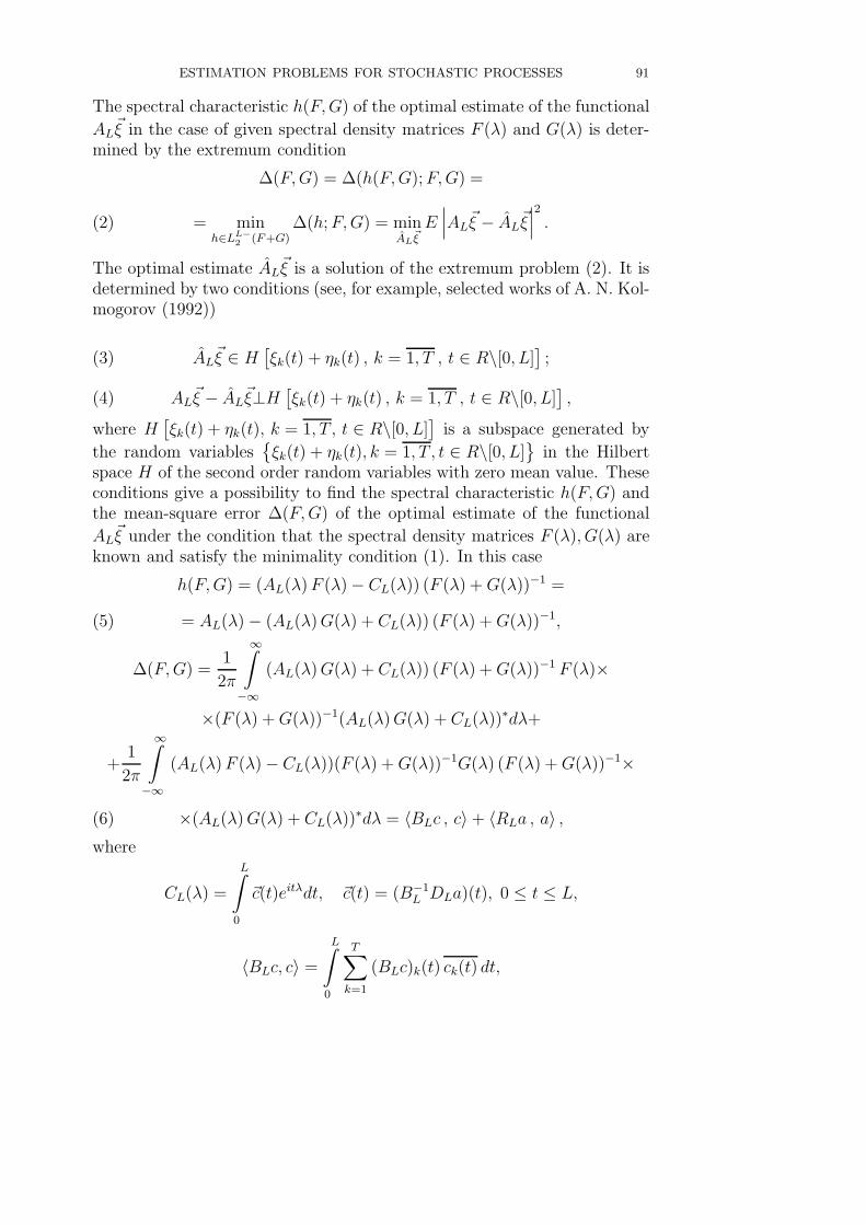
The spectral characteristic h(F, G) of the optimal estimate of the functional
AL�ξ in the case of given spectral density matrices F (λ) and G(λ) is deter-
mined by the extremum condition
Δ(F, G) = Δ(h(F, G); F, G) =
(2) = minh∈LL−
2 (F+G)Δ(h; F, G) = min
AL�ξE∣∣∣AL
�ξ − AL�ξ∣∣∣2 .
The optimal estimate AL�ξ is a solution of the extremum problem (2). It is
determined by two conditions (see, for example, selected works of A. N. Kol-mogorov (1992))
(3) AL�ξ ∈ H
[ξk(t) + ηk(t) , k = 1, T , t ∈ R\[0, L]
];
(4) AL�ξ − AL
�ξ⊥H[ξk(t) + ηk(t) , k = 1, T , t ∈ R\[0, L]
],
where H[ξk(t) + ηk(t), k = 1, T , t ∈ R\[0, L]
]is a subspace generated by
the random variables{ξk(t) + ηk(t), k = 1, T , t ∈ R\[0, L]
}in the Hilbert
space H of the second order random variables with zero mean value. Theseconditions give a possibility to find the spectral characteristic h(F, G) andthe mean-square error Δ(F, G) of the optimal estimate of the functional
AL�ξ under the condition that the spectral density matrices F (λ), G(λ) are
known and satisfy the minimality condition (1). In this case
h(F, G) = (AL(λ) F (λ) − CL(λ)) (F (λ) + G(λ))−1 =
(5) = AL(λ) − (AL(λ) G(λ) + CL(λ)) (F (λ) + G(λ))−1,
Δ(F, G) =1
2π
∞∫−∞
(AL(λ) G(λ) + CL(λ)) (F (λ) + G(λ))−1 F (λ)×
×(F (λ) + G(λ))−1(AL(λ) G(λ) + CL(λ))∗dλ+
+1
2π
∞∫−∞
(AL(λ) F (λ) − CL(λ))(F (λ) + G(λ))−1G(λ) (F (λ) + G(λ))−1×
(6) ×(AL(λ) G(λ) + CL(λ))∗dλ = 〈BLc , c〉 + 〈RLa , a〉 ,
where
CL(λ) =
L∫0
�c(t)eitλdt, �c(t) = (B−1L DLa)(t), 0 ≤ t ≤ L,
〈BLc, c〉 =
L∫0
T∑k=1
(BLc)k(t) ck(t) dt,
92 MIKHAIL MOKLYACHUK AND ALEKSANDR MASYUTKA
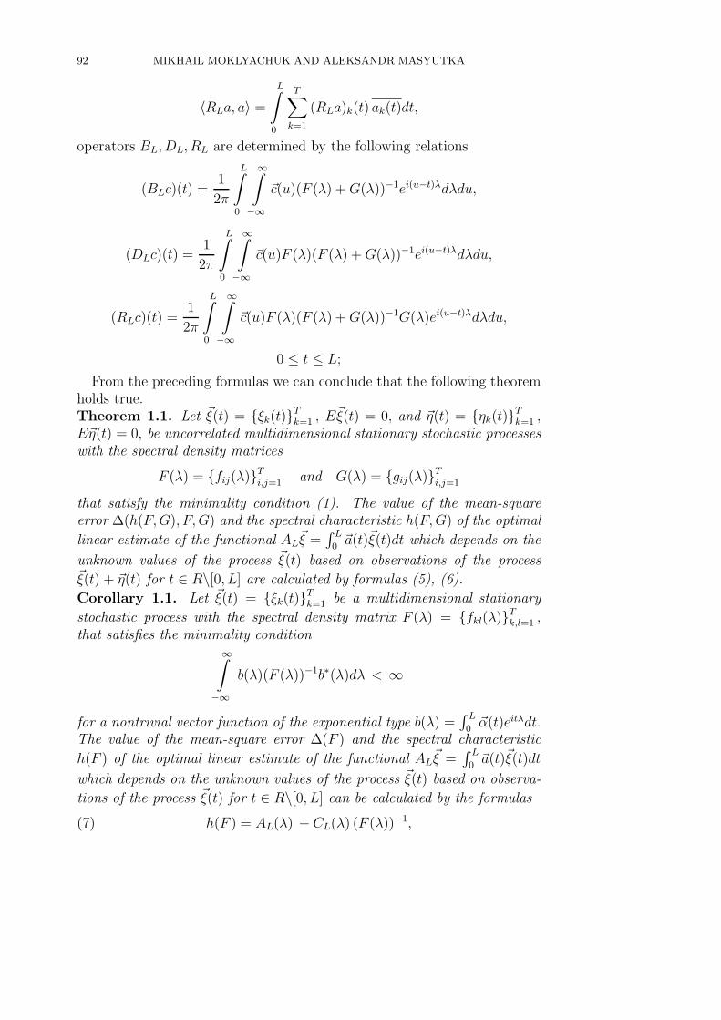
〈RLa, a〉 =
L∫0
T∑k=1
(RLa)k(t) ak(t)dt,
operators BL, DL, RL are determined by the following relations
(BLc)(t) =1
2π
L∫0
∞∫−∞
�c(u)(F (λ) + G(λ))−1ei(u−t)λdλdu,
(DLc)(t) =1
2π
L∫0
∞∫−∞
�c(u)F (λ)(F (λ) + G(λ))−1ei(u−t)λdλdu,
(RLc)(t) =1
2π
L∫0
∞∫−∞
�c(u)F (λ)(F (λ) + G(λ))−1G(λ)ei(u−t)λdλdu,
0 ≤ t ≤ L;
From the preceding formulas we can conclude that the following theoremholds true.Theorem 1.1. Let �ξ(t) = {ξk(t)}T
k=1 , E�ξ(t) = 0, and �η(t) = {ηk(t)}Tk=1 ,
E�η(t) = 0, be uncorrelated multidimensional stationary stochastic processeswith the spectral density matrices
F (λ) = {fij(λ)}Ti,j=1 and G(λ) = {gij(λ)}T
i,j=1
that satisfy the minimality condition (1). The value of the mean-squareerror Δ(h(F, G), F, G) and the spectral characteristic h(F, G) of the optimal
linear estimate of the functional AL�ξ =
∫ L
0�a(t)�ξ(t)dt which depends on the
unknown values of the process �ξ(t) based on observations of the process�ξ(t) + �η(t) for t ∈ R\[0, L] are calculated by formulas (5), (6).
Corollary 1.1. Let �ξ(t) = {ξk(t)}Tk=1 be a multidimensional stationary
stochastic process with the spectral density matrix F (λ) = {fkl(λ)}Tk,l=1 ,
that satisfies the minimality condition∞∫
−∞
b(λ)(F (λ))−1b∗(λ)dλ < ∞
for a nontrivial vector function of the exponential type b(λ) =∫ L
0�α(t)eitλdt.
The value of the mean-square error Δ(F ) and the spectral characteristic
h(F ) of the optimal linear estimate of the functional AL�ξ =
∫ L
0�a(t)�ξ(t)dt
which depends on the unknown values of the process �ξ(t) based on observa-
tions of the process �ξ(t) for t ∈ R\[0, L] can be calculated by the formulas
(7) h(F ) = AL(λ) − CL(λ) (F (λ))−1,
ESTIMATION PROBLEMS FOR STOCHASTIC PROCESSES 93
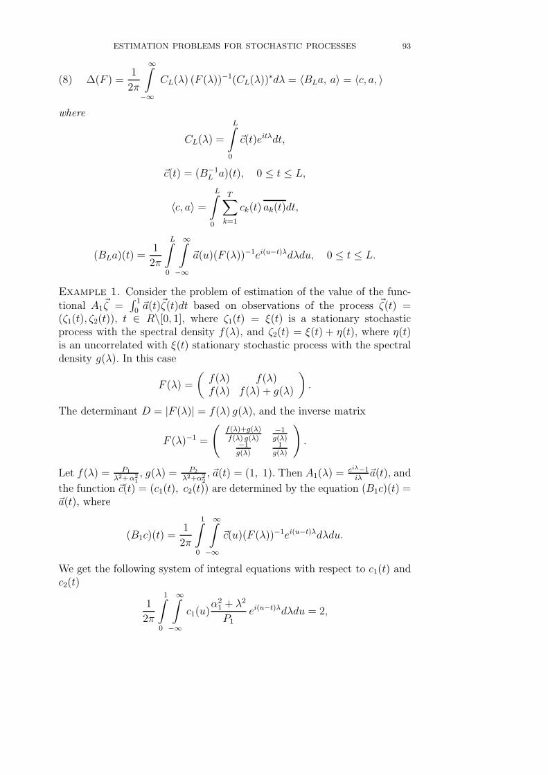
(8) Δ(F ) =1
2π
∞∫−∞
CL(λ) (F (λ))−1(CL(λ))∗dλ = 〈BLa, a〉 = 〈c, a, 〉
where
CL(λ) =
L∫0
�c(t)eitλdt,
�c(t) = (B−1L a)(t), 0 ≤ t ≤ L,
〈c, a〉 =
L∫0
T∑k=1
ck(t) ak(t)dt,
(BLa)(t) =1
2π
L∫0
∞∫−∞
�a(u)(F (λ))−1ei(u−t)λdλdu, 0 ≤ t ≤ L.
Example 1. Consider the problem of estimation of the value of the func-
tional A1�ζ =
∫ 1
0�a(t)�ζ(t)dt based on observations of the process �ζ(t) =
(ζ1(t), ζ2(t)), t ∈ R\[0, 1], where ζ1(t) = ξ(t) is a stationary stochasticprocess with the spectral density f(λ), and ζ2(t) = ξ(t) + η(t), where η(t)is an uncorrelated with ξ(t) stationary stochastic process with the spectraldensity g(λ). In this case
F (λ) =
(f(λ) f(λ)f(λ) f(λ) + g(λ)
).
The determinant D = |F (λ)| = f(λ) g(λ), and the inverse matrix
F (λ)−1 =
(f(λ)+g(λ)f(λ) g(λ)
−1g(λ)
−1g(λ)
1g(λ)
).
Let f(λ) = P1
λ2+ α21, g(λ) = P2
λ2+α22, �a(t) = (1, 1). Then A1(λ) = eiλ−1
iλ�a(t), and
the function �c(t) = (c1(t), c2(t)) are determined by the equation (B1c)(t) =�a(t), where
(B1c)(t) =1
2π
1∫0
∞∫−∞
�c(u)(F (λ))−1ei(u−t)λdλdu.
We get the following system of integral equations with respect to c1(t) andc2(t)
1
2π
1∫0
∞∫−∞
c1(u)α2
1 + λ2
P1ei(u−t)λdλdu = 2,
94 MIKHAIL MOKLYACHUK AND ALEKSANDR MASYUTKA
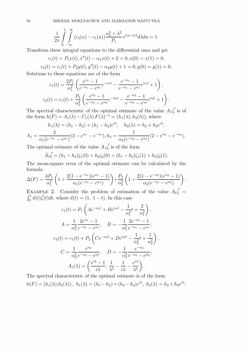
1
2π
1∫0
∞∫−∞
(c2(u) − c1(u))α2
2 + λ2
P1
ei(u−t)λdλdu = 1.
Transform these integral equations to the differential ones and get
c1(t) = P1x(t), x′′(t) − α1x(t) + 2 = 0, x(0) = x(1) = 0,
c2(t) = c1(t) + P2y(t), y′′(t) − α2y(t) + 1 = 0, y(0) = y(1) = 0.
Solutions to these equations are of the form
c1(t) =2P1
α21
(eα1 − 1
e−α1 − eα1e−α1t − e−α1 − 1
e−α1 − eα1eα1t + 1
),
c2(t) = c1(t) +P2
α22
(eα2 − 1
e−α2 − eα2e−α2t − e−α2 − 1
e−α2 − eα2eα2t + 1
).
The spectral characteristic of the optimal estimate of the value A1�ζ is of
the form h(F ) = A1(λ) − C1(λ) F (λ)−1 = (h1(λ), h2(λ)), where
h1(λ) = (h1 − h2) + (h1 − h2)eiλ, h2(λ) = h2 + h2e
iλ,
h1 =2
α1(e−α1 − eα1)(2 − eα1 − e−α1), h2 =
1
α2(e−α2 − eα2)(2 − eα2 − e−α2).
The optimal estimate of the value A1�ζ is of the form
A1�ζ = (h1 − h2)ζ1(0) + h2ζ2(0) + (h1 − h2)ζ1(1) + h2ζ2(1).
The mean-square error of the optimal estimate can be calculated by theformula
Δ(F ) =4P1
α21
(1 +
2(1 − e−α1)(eα1 − 1)
α1(e−α1 − eα1)
)+
P2
α22
(1 +
2(1 − e−α2)(eα2 − 1)
α2(e−α2 − eα2)
).
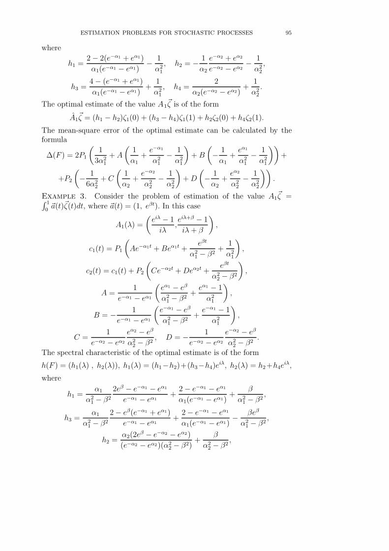
Example 2. Consider the problem of estimation of the value A1�ζ =∫ 1
0�a(t)�ζ(t)dt, where �a(t) = (1, 1 − t). In this case
c1(t) = P1
(Ae−α1t + Beα1t − 1
α21
t +2
α21
),
A =1
α21
2eα1 − 1
e−α1 − eα1, B = − 1
α21
2e−α1 − 1
e−α1 − eα1;
c2(t) = c1(t) + P2
(Ce−α2t + Deα2t − 1
α22
t +1
α22
),
C =1
α22
eα2
e−α2 − eα2, D = − 1
α22
e−α2
e−α2 − eα2;
A1(λ) =
(eiλ − 1
iλ,
1
λ2− 1
iλ− eiλ
λ2
).
The spectral characteristic of the optimal estimate is of the form
h(F ) = (h1(λ),h2(λ)) , h1(λ) = (h1 −h2)+ (h3 −h4)eiλ, h2(λ) = h2 +h4e
iλ,
ESTIMATION PROBLEMS FOR STOCHASTIC PROCESSES 95
where
h1 =2 − 2(e−α1 + eα1)
α1(e−α1 − eα1)− 1
α21
, h2 = − 1
α2
e−α2 + eα2
e−α2 − eα2− 1
α22
,
h3 =4 − (e−α1 + eα1)
α1(e−α1 − eα1)+
1
α21
, h4 =2
α2(e−α2 − eα2)+
1
α22
.
The optimal estimate of the value A1�ζ is of the form
A1�ζ = (h1 − h2)ζ1(0) + (h3 − h4)ζ1(1) + h2ζ2(0) + h4ζ2(1).
The mean-square error of the optimal estimate can be calculated by theformula
Δ(F ) = 2P1
(1
3α21
+ A
(1
α1+
e−α1
α21
− 1
α21
)+ B
(− 1
α1+
eα1
α21
− 1
α21
))+
+P2
(− 1
6α22
+ C
(1
α2+
e−α2
α22
− 1
α22
)+ D
(− 1
α2+
eα2
α22
− 1
α22
)).
Example 3. Consider the problem of estimation of the value A1�ζ =∫ 1
0�a(t)�ζ(t)dt, where �a(t) = (1, eβt). In this case
A1(λ) =
(eiλ − 1
iλ,eiλ+β − 1
iλ + β
),
c1(t) = P1
(Ae−α1t + Beα1t +
eβt
α21 − β2
+1
α21
),
c2(t) = c1(t) + P2
(Ce−α2t + Deα2t +
eβt
α22 − β2
),
A =1
e−α1 − eα1
(eα1 − eβ
α21 − β2
+eα1 − 1
α21
),
B = − 1
e−α1 − eα1
(e−α1 − eβ
α21 − β2
+e−α1 − 1
α21
),
C =1
e−α2 − eα2
eα2 − eβ
α22 − β2
, D = − 1
e−α2 − eα2
e−α2 − eβ
α22 − β2
.
The spectral characteristic of the optimal estimate is of the form
h(F ) = (h1(λ) , h2(λ)), h1(λ) = (h1−h2)+(h3−h4)eiλ, h2(λ) = h2+h4e
iλ,
where
h1 =α1
α21 − β2
2eβ − e−α1 − eα1
e−α1 − eα1+
2 − e−α1 − eα1
α1(e−α1 − eα1)+
β
α21 − β2
,
h3 =α1
α21 − β2
2 − eβ(e−α1 + eα1)
e−α1 − eα1+
2 − e−α1 − eα1
α1(e−α1 − eα1)− βeβ
α21 − β2
,
h2 =α2(2e
β − e−α2 − eα2)
(e−α2 − eα2)(α22 − β2)
+β
α22 − β2
,
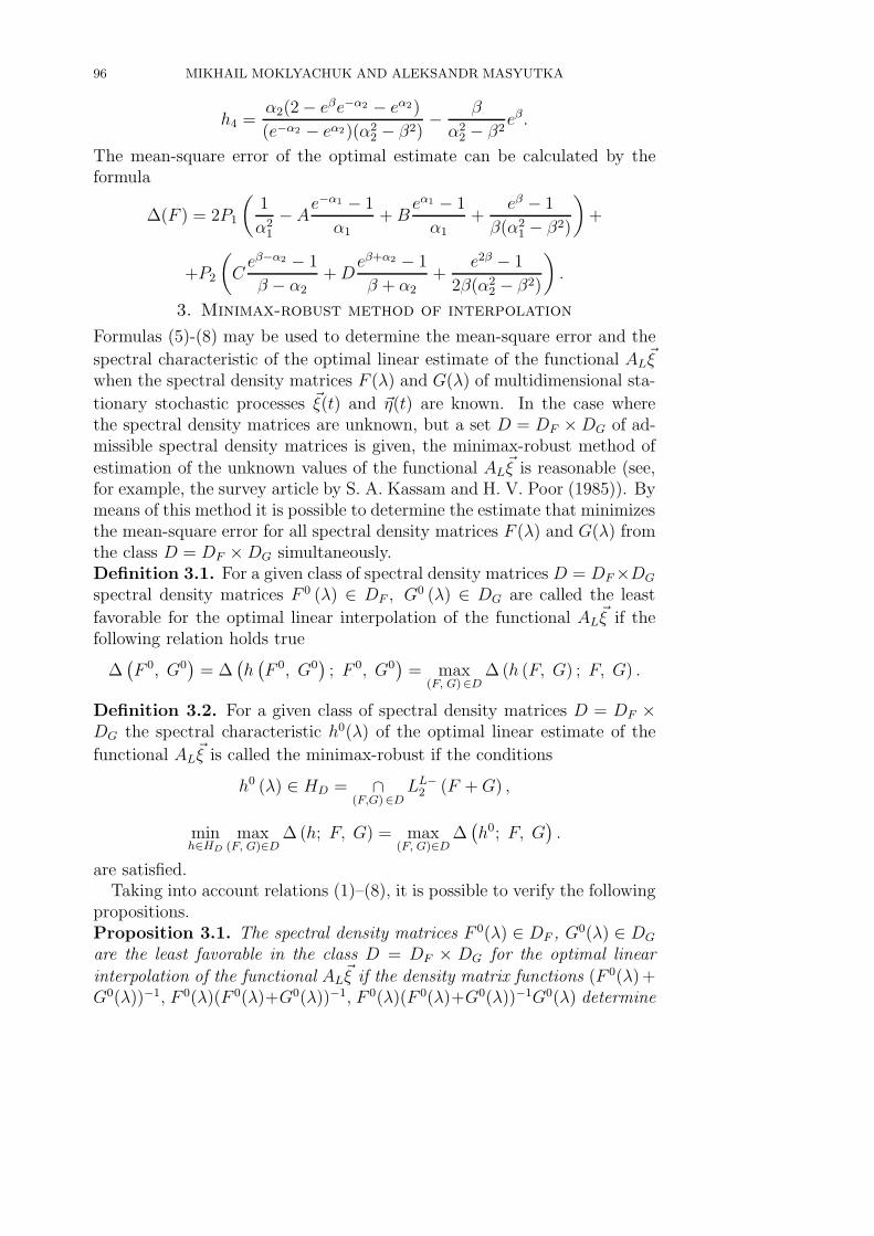
96 MIKHAIL MOKLYACHUK AND ALEKSANDR MASYUTKA
h4 =α2(2 − eβe−α2 − eα2)
(e−α2 − eα2)(α22 − β2)
− β
α22 − β2
eβ.
The mean-square error of the optimal estimate can be calculated by theformula
Δ(F ) = 2P1
(1
α21
− Ae−α1 − 1
α1+ B
eα1 − 1
α1+
eβ − 1
β(α21 − β2)
)+
+P2
(C
eβ−α2 − 1
β − α2+ D
eβ+α2 − 1
β + α2+
e2β − 1
2β(α22 − β2)
).
3. Minimax-robust method of interpolation
Formulas (5)-(8) may be used to determine the mean-square error and the
spectral characteristic of the optimal linear estimate of the functional AL�ξ
when the spectral density matrices F (λ) and G(λ) of multidimensional sta-
tionary stochastic processes �ξ(t) and �η(t) are known. In the case wherethe spectral density matrices are unknown, but a set D = DF × DG of ad-missible spectral density matrices is given, the minimax-robust method of
estimation of the unknown values of the functional AL�ξ is reasonable (see,
for example, the survey article by S. A. Kassam and H. V. Poor (1985)). Bymeans of this method it is possible to determine the estimate that minimizesthe mean-square error for all spectral density matrices F (λ) and G(λ) fromthe class D = DF × DG simultaneously.Definition 3.1. For a given class of spectral density matrices D = DF ×DG
spectral density matrices F 0 (λ) ∈ DF , G0 (λ) ∈ DG are called the least
favorable for the optimal linear interpolation of the functional AL�ξ if the
following relation holds true
Δ(F 0, G0
)= Δ
(h(F 0, G0
); F 0, G0
)= max
(F, G)∈DΔ (h (F, G) ; F, G) .
Definition 3.2. For a given class of spectral density matrices D = DF ×DG the spectral characteristic h0(λ) of the optimal linear estimate of the
functional AL�ξ is called the minimax-robust if the conditions
h0 (λ) ∈ HD = ∩(F,G)∈D
LL−2 (F + G) ,
minh∈HD
max(F, G)∈D
Δ (h; F, G) = max(F, G)∈D
Δ(h0; F, G
).
are satisfied.Taking into account relations (1)–(8), it is possible to verify the following
propositions.Proposition 3.1. The spectral density matrices F 0(λ) ∈ DF , G0(λ) ∈ DG
are the least favorable in the class D = DF × DG for the optimal linear
interpolation of the functional AL�ξ if the density matrix functions (F 0(λ)+
G0(λ))−1, F 0(λ)(F 0(λ)+G0(λ))−1, F 0(λ)(F 0(λ)+G0(λ))−1G0(λ) determine

ESTIMATION PROBLEMS FOR STOCHASTIC PROCESSES 97
operators B0L, D0
L, R0L, which give solutions to the conditional extremum
problem(9)
max(F, G)∈D
(⟨DLa, B−1
L DLa⟩
+ 〈RLa, a〉) =⟨D0
La, (B0L)−1D0
La⟩
+⟨R0
La, a⟩.
The minimax-robust spectral characteristic h0 = h(F 0, G0) of the optimal
linear estimate of the functional AL�ξ can be calculated by formula (5) if the
condition h(F 0, G0) ∈ HD holds true.Proposition 3.2. The spectral density matrix F 0(λ) ∈ DF which satisfiesthe minimality condition is the least favorable in the class D = DF for the
optimal linear interpolation of the functional AL�ξ based on observations of
�ξ(t), t ∈ R\[0, L], if the density matrix function (F 0(λ))−1 determine theoperator B0
L which gives a solution to the conditional extremum problem
(10) maxF∈DF
⟨(BL)−1a, a
⟩=⟨(B0
L)−1a, a⟩.
The minimax-robust spectral characteristic h0 = h(F 0) of the optimal lin-
ear estimate of the functional AL�ξ can be calculated by formula (7) if the
condition h(F 0) ∈ HD holds true.The least favorable spectral density matrices F 0(λ) ∈ D, G0(λ) ∈ DG
and the minimax-robust spectral characteristic h0 = h (F 0, G0) ∈ HD forma saddle point of the function Δ(h; F, G) on the set HD × D. The saddlepoint inequalities
Δ(h0; F, G
) ≤ Δ(h0; F 0, G0
) ≤ Δ(h; F 0, G0
),
∀h ∈ HD, ∀F ∈ DF , ∀G ∈ DG
hold true if h0 = h(F 0, G0) ∈ HD and (F 0, G0) give a solution to theconditional extremum problem
(11) sup(F,G)∈D
Δ(h(F 0, G0
); F, G
)= Δ
(h(F 0, G0
); F 0, G0
),
where
Δ(h(F 0, G0
); F, G
)=
=1
2π
∞∫−∞
(AL(λ) G0(λ) + C0L(λ)) (F 0(λ) + G0(λ))−1 F (λ)×
×(F 0(λ) + G0(λ))−1(AL(λ) G0(λ) + C0L(λ))∗dλ+
+1
2π
∞∫−∞
(AL(λ) F 0(λ) − C0L(λ))(F 0(λ) + G0(λ))−1G(λ)×
×(F 0(λ) + G0(λ))−1(AL(λ) G0(λ) + C0L(λ))∗dλ.
98 MIKHAIL MOKLYACHUK AND ALEKSANDR MASYUTKA
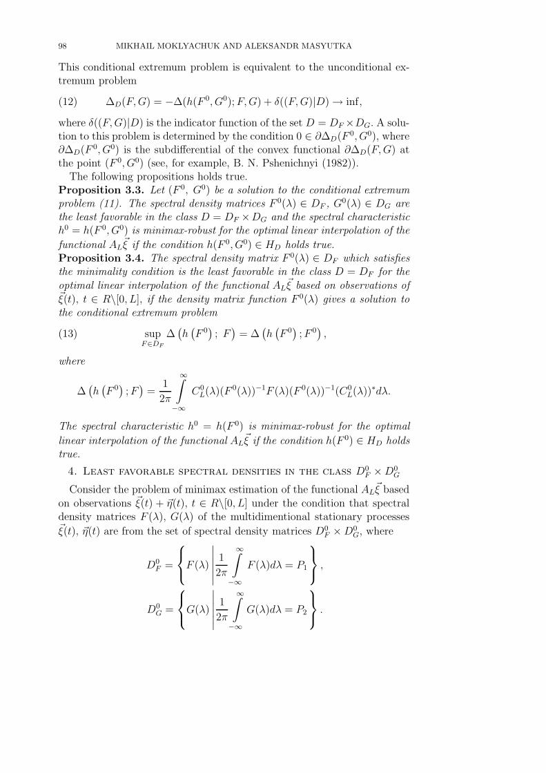
This conditional extremum problem is equivalent to the unconditional ex-tremum problem
(12) ΔD(F, G) = −Δ(h(F 0, G0); F, G) + δ((F, G)|D) → inf,
where δ((F, G)|D) is the indicator function of the set D = DF ×DG. A solu-tion to this problem is determined by the condition 0 ∈ ∂ΔD(F 0, G0), where∂ΔD(F 0, G0) is the subdifferential of the convex functional ∂ΔD(F, G) atthe point (F 0, G0) (see, for example, B. N. Pshenichnyi (1982)).
The following propositions holds true.Proposition 3.3. Let (F 0, G0) be a solution to the conditional extremumproblem (11). The spectral density matrices F 0(λ) ∈ DF , G0(λ) ∈ DG arethe least favorable in the class D = DF ×DG and the spectral characteristich0 = h(F 0, G0) is minimax-robust for the optimal linear interpolation of the
functional AL�ξ if the condition h(F 0, G0) ∈ HD holds true.
Proposition 3.4. The spectral density matrix F 0(λ) ∈ DF which satisfiesthe minimality condition is the least favorable in the class D = DF for the
optimal linear interpolation of the functional AL�ξ based on observations of
�ξ(t), t ∈ R\[0, L], if the density matrix function F 0(λ) gives a solution tothe conditional extremum problem
(13) supF∈DF
Δ(h(F 0); F
)= Δ
(h(F 0); F 0
),
where
Δ(h(F 0); F)
=1
2π
∞∫−∞
C0L(λ)(F 0(λ))−1F (λ)(F 0(λ))−1(C0
L(λ))∗dλ.
The spectral characteristic h0 = h(F 0) is minimax-robust for the optimal
linear interpolation of the functional AL�ξ if the condition h(F 0) ∈ HD holds
true.
4. Least favorable spectral densities in the class D0F × D0
G
Consider the problem of minimax estimation of the functional AL�ξ based
on observations �ξ(t) + �η(t), t ∈ R\[0, L] under the condition that spectraldensity matrices F (λ), G(λ) of the multidimentional stationary processes�ξ(t), �η(t) are from the set of spectral density matrices D0
F × D0G, where
D0F =
⎧⎨⎩F (λ)
∣∣∣∣∣∣1
2π
∞∫−∞
F (λ)dλ = P1
⎫⎬⎭ ,
D0G =
⎧⎨⎩G(λ)
∣∣∣∣∣∣1
2π
∞∫−∞
G(λ)dλ = P2
⎫⎬⎭ .
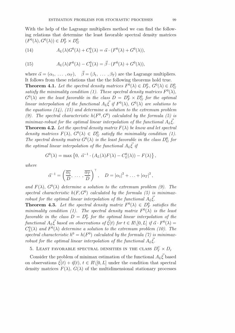
ESTIMATION PROBLEMS FOR STOCHASTIC PROCESSES 99
With the help of the Lagrange multipliers method we can find the follow-ing relations that determine the least favorable spectral density matrices
(F 0(λ), G0(λ)) ∈ D0F × D0
G
(14) AL(λ)G0(λ) + C0L(λ) = �α · (F 0(λ) + G0(λ)),
(15) AL(λ)F 0(λ) − C0L(λ) = �β · (F 0(λ) + G0(λ)),
where �α = (α1, . . . , αT ), �β = (β1, . . . , βT ) are the Lagrange multipliers.
It follows from these relations that the the following theorems hold true.Theorem 4.1. Let the spectral density matrices F 0(λ) ∈ D0
F , G0(λ) ∈ D0G
satisfy the minimality condition (1). These spectral density matrices F 0(λ),
G0(λ) are the least favorable in the class D = D0F × D0
G for the optimal
linear interpolation of the functional AL�ξ if F 0(λ), G0(λ) are solutions to
the equations (14), (15) and determine a solution to the extremum problem(9). The spectral characteristic h(F 0, G0) calculated by the formula (5) is
minimax-robust for the optimal linear interpolation of the functional AL�ξ.
Theorem 4.2. Let the spectral density matrix F (λ) be know and let spectraldensity matrices F (λ), G0(λ) ∈ D0
G satisfy the minimality condition (1).
The spectral density matrix G0(λ) is the least favorable in the class D0G for
the optimal linear interpolation of the functional AL�ξ if
G0(λ) = max{0, �α−1 · (AL(λ)F (λ) − C0
L(λ)) − F (λ)}
,
where
�α−1 =
(α1
D, . . . ,
αT
D
)�, D = |α1|2 + . . . + |αT |2 ,
and F (λ), G0(λ) determine a solution to the extremum problem (9). Thespectral characteristic h(F, G0) calculated by the formula (5) is minimax-
robust for the optimal linear interpolation of the functional AL�ξ.
Theorem 4.3. Let the spectral density matrix F 0(λ) ∈ D0F satisfies the
minimality condition (1). The spectral density matrix F 0(λ) is the least
favorable in the class D = D0F for the optimal linear interpolation of the
functional AL�ξ based on observations of �ξ(t) for t ∈ R\[0, L] if �α · F 0(λ) =
C0L(λ) and F 0(λ) determine a solution to the extremum problem (10). The
spectral characteristic h0 = h(F 0) calculated by the formula (7) is minimax-
robust for the optimal linear interpolation of the functional AL�ξ.
5. Least favorable spectral densities in the class DUV × Dε
Consider the problem of minimax estimation of the functional AL�ξ based
on observations �ξ(t) + �η(t), t ∈ R\[0, L] under the condition that spectral
density matrices F (λ), G(λ) of the multidimensional stationary processes
100 MIKHAIL MOKLYACHUK AND ALEKSANDR MASYUTKA
�ξ(t), �η(t) are from the set of spectral density matrices DUV × Dε, where
DUV =
⎧⎨⎩F (λ)
∣∣∣∣∣∣V (λ) ≤ F (λ) ≤ U(λ),1
2π
∞∫−∞
F (λ)dλ = P1
⎫⎬⎭ ,
Dε =
⎧⎨⎩G(λ)
∣∣∣∣∣∣G(λ) = (1 − ε)G1(λ) + εW (λ),1
2π
∞∫−∞
G(λ)dλ = P2
⎫⎬⎭ ,
where V (λ), U(λ), G1(λ) are given fixed spectral density matrices, W (λ)ia an unknown spectral density matrix, and expression B(λ) ≥ D(λ) meansthat B(λ) − D(λ) ≥ 0 (positive definite matrix function). The set DU
V
describes the ‘band’ model of stochastic processes while the set Dε describesthe ‘ε-contaminated’ model of stochastic processes. For the set DU
V × Dε
from the condition 0 ∈ ∂ΔD(F 0, G0) we can get the following relationswhich determine the least favorable spectral density matrices
(16) �a0(λ)�a0(λ)∗ = �α · �α∗ + Γ1(λ) + Γ2(λ);
(17) �b0(λ)�b0(λ)∗ = �β · �β∗ + Γ3(λ),
where�a0(λ) =
((AL(λ)G0(λ) + C0
L(λ))(F 0(λ) + G0(λ))−1)T
,
�b0(λ) =((AL(λ)F 0(λ) − C0
L(λ))(F 0(λ) + G0(λ))−1)T
.
The coefficients �α = (α1, . . . , αT )T , �β = (β1, . . . βT )T are determined by theconditions
(18)1
2π
∞∫−∞
F 0(λ)dλ = P1,1
2π
∞∫−∞
G0(λ)dλ = P2.
The matrix functions Γ1(λ) ≥ 0, Γ2(λ) ≥ 0, Γ3(λ) ≥ 0 are determined bythe conditions
(19) V (λ) ≤ F 0(λ) ≤ U(λ), G0(λ) = (1 − ε)G1(λ) + εW (λ),
(20) Γ1(λ) = 0 if F 0(λ) ≥ V (λ), Γ2(λ) = 0 if F 0(λ) ≤ U(λ),
(21) Γ3(λ) = 0 if G0(λ) ≥ (1 − ε)G1(λ).
It follows from these relations that the the following theorems hold true.Theorem 5.1. Let the spectral density matrices F 0(λ) ∈ DU
V , G0(λ) ∈Dε satisfy the minimality condition (1). These spectral density matricesF 0(λ), G0(λ) are the least favorable in the class DU
V × Dε for the optimal
linear interpolation of the functional AL�ξ if they satisfy conditions (16) –
(21) and determine a solution to the extremum problem (9). The spectral
ESTIMATION PROBLEMS FOR STOCHASTIC PROCESSES 101
characteristic h(F 0, G0) calculated by the formula (5) is minimax-robust for
the optimal linear interpolation of the functional AL�ξ.
Theorem 5.2. Let the spectral density matrix F (λ) be known and let spec-tral density matrices F (λ), G0(λ) ∈ Dε satisfy the minimality condition (1).The spectral density matrix G0(λ) is the least favorable in the class Dε for
the optimal linear interpolation of the functional AL�ξ if
G0(λ) = max{(1 − ε)G1(λ), �α−1(AL(λ)F (λ) − C0
L(λ)) − G(λ)}
and (F (λ), G0(λ)) determine a solution to the extremum problem (9). Thespectral characteristic h(F, G0) calculated by the formula (5) is minimax-
robust for the optimal linear interpolation of the functional AL�ξ.
Theorem 5.3. Let the spectral density matrix F 0(λ) ∈ DUV satisfies the
minimality condition (1). This spectral density matrix F 0(λ) is the leastfavorable in the class D = DU
V for the optimal linear interpolation of the
functional AL�ξ based on observations of �ξ(t) for t ∈ R\[0, L] if
F 0(λ) = max{V (λ), min
{U(λ), �α−1C0
L(λ)}}
and F 0(λ) determine a solution to the extremum problem (10). The spectralcharacteristic h0 = h(F 0) calculated by the formula (7) is minimax-robust
for the optimal linear interpolation of the functional AL�ξ.
6. Hilbert space projection method of extrapolation
Let the vector function �a(t) which determines the functional A�ξ satisfiesconditions:
(22)
∫ ∞
0
T∑k=1
|ak(t)| dt < ∞,
∫ ∞
0
t
T∑k=1
|ak(t)|2dt < ∞.
Under these conditions the functional A�ξ has the second moment and theoperator A defined below is compact.
Let the spectral density matrices
F (λ) = {fkl(λ)}Tk,l=1 and G(λ) = {gkl(λ)}T
k,l=1
of uncorrelated multidimensional stationary stochastic processes �ξ(t) =
{ξk(t)}Tk=1 , �η(t) = {ηk(t)}T
k=1 satisfy the minimality condition (1), where
b(λ) =∫∞0
�α(t)eitλdt, �α(t) = {αk(t)}Tk=1, is a nontrivial vector function of
the exponential type.Denote by L−
2 (F ) the subspace in L2(F ), generated by functions eitλδk,
t < 0, δk = {δkl}Tl=1 , k = 1, . . . , T , where δkk = 1, δkl = 0 for k �= l. Any
linear linear extrapolation A�ξ of the functional A�ξ based on observations of
the process �ξ(t) + �η(t) for t < 0 is of the form
A�ξ =
∞∫−∞
h(λ) (Zξ(dλ) + Zη(dλ)) =
∞∫−∞
T∑k=1
hk(λ)(Zξk(dλ) + Zη
k (dλ)),
102 MIKHAIL MOKLYACHUK AND ALEKSANDR MASYUTKA
where h(λ) = {hk(λ)}Tk=1 is the spectral characteristic of the linear extrap-
olation A�ξ. The function h(λ) ∈ L−2 (F + G). The value of the mean square
error Δ(h; F, G) of the linear extrapolation A�ξ is calculated by the formula
Δ(h; F, G) = E∣∣∣A�ξ − A�ξ
∣∣∣2 =
1
2π
∞∫−∞
(A(λ) − h(λ)) F (λ) (A(λ)− h(λ))∗dλ +1
2π
∞∫−∞
h(λ) G(λ) h∗(λ)dλ,
where
A(λ) =
∞∫0
�a(t)eitλdt.
The spectral characteristic h(F, G) of the optimal linear linear extrapolation
of A�ξ minimizes the mean square error
Δ(F, G) = Δ(h(F, G); F, G)
(23) = minh∈L−
2 (F+G)Δ(h; F, G) = min
A�ξE∣∣∣A�ξ − A�ξ
∣∣∣2 .
With the help of the Hilbert space projection method proposed by A. N. Kol-mogorov we can find a solution of the optimization problem (23):
h(F, G) = (A(λ) F (λ) − C(λ)) (F (λ) + G(λ))−1 =
(24) = A(λ) − (A(λ) G(λ) + C(λ)) (F (λ) + G(λ))−1,
Δ(F, G) =1
2π
∞∫−∞
(A(λ) G(λ) + C(λ)) (F (λ) + G(λ))−1 F (λ)×
×(F (λ) + G(λ))−1(A(λ) G(λ) + C(λ))∗dλ+
+1
2π
∞∫−∞
(A(λ) F (λ) − C(λ))(F (λ) + G(λ))−1G(λ) (F (λ) + G(λ))−1×
(25) ×(A(λ) G(λ) + C(λ))∗dλ = 〈Bc , c〉 + 〈Ra , a〉 ,
where
C(λ) =
∞∫0
�c(t)eitλdt, �c(t) = (B−1Da)(t),
〈Bc, c〉 =
∞∫0
n∑k=1
(Bc)k(t) ck(t) dt,
ESTIMATION PROBLEMS FOR STOCHASTIC PROCESSES 103
〈Ra, a〉 =
∞∫0
n∑k=1
(Ra)k(t) ak(t)dt,
operators B,D,R are determined by the following relations
(Bc)(t) =1
2π
∞∫0
∞∫−∞
�c(u)(F (λ) + G(λ))−1ei(u−t)λdλdu,
(Dc)(t) =1
2π
∞∫0
∞∫−∞
�c(u)F (λ)(F (λ) + G(λ))−1ei(u−t)λdλdu,
(Rc)(t) =1
2π
∞∫0
∞∫−∞
�c(u)F (λ)(F (λ) + G(λ))−1G(λ)ei(u−t)λdλdu.
From the preceding formulas we can conclude that the following theoremholds true.Theorem 6.1. Let �ξ(t) = {ξk(t)}T
k=1 and �η(t) = {ηk(t)}Tk=1 be uncorrelated
multidimensional stationary stochastic processes with the spectral densitymatrices F (λ) = {fij(λ)}T
i,j=1 and G(λ) = {gij(λ)}Ti,j=1 that satisfy the min-
imality condition (1). Let condition (22) be satisfied. The value of themean-square error Δ(h(F, G), F, G) and the spectral characteristic h(F, G)
of the optimal linear extrapolation of the functional A�ξ =∫∞0
�a(t)�ξ(t)dt
which depends on the unknown values of the process �ξ(t) t ≥ 0, based on
observations of the process �ξ(t) + �η(t) for t < 0 are calculated by formulas(24), (25).
Corollary 6.1. Let �ξ(t) = {ξk(t)}Tk=1 be a multidimensional stationary
stochastic process with the spectral density matrix F (λ) = {fkl(λ)}Tk,l=1 ,
that satisfies the minimality condition∞∫
−∞
b(λ)(F (λ))−1b∗(λ)dλ < ∞
for a nontrivial vector function of the exponential type b(λ) =∫∞
0�α(t)eitλdt.
Let condition (22) be satisfied. The value of the mean-square error Δ(F )and the spectral characteristic h(F ) of the optimal linear extrapolation of
the functional A�ξ =∫∞0
�a(t)�ξ(t)dt based on observations of the process �ξ(t)for t < 0 are calculated by the formulas
(26) h(F ) = A(λ) − C(λ) (F (λ))−1,
(27) Δ(F ) =1
2π
∞∫−∞
C(λ) (F (λ))−1(C(λ))∗dλ = 〈Ba, a〉 = 〈c, a〉
104 MIKHAIL MOKLYACHUK AND ALEKSANDR MASYUTKA
where �c(t) = (B−1a)(t),
(Ba)(t) =1
2π
∞∫0
∞∫−∞
�a(u)(F (λ))−1ei(u−t)λdλdu.
Let the process �ξ(t) admits the canonical moving average representation
(28) �ξ(t) =
∫ t
−∞d(t − u) d�ε(u),
where d(s) = {dij(s)}j=1,m
i=1,Tis a matrix function and �ε(u) = {εk(u)}m
k=1 is
a multidimensional stationary stochastic process with uncorrelated incre-ments. In this case the spectral density matrix F (λ) = {fij(λ)}n
i,j=1 of the
process �ξ(t) admits the canonical factorization:
(29) F (λ) = ϕ(λ) ϕ∗(λ), ϕ(λ) =
∫ ∞
0
d(u)e−iuλdλ.
If the process �ξ(t) admits the canonical moving average representation (28),
then the optimal linear extrapolation of the functional A�ξ =∫∞0
�a(t)�ξ(t)dt
based on observations of the process �ξ(t) for t < 0 is determined by thespectral characteristic h(F ) ∈ L−
2 (F ) that minimizes the mean square error
(30) Δ(h(F ), F ) = minh∈L−
2 (F )Δ(h, F ) = ‖Ad‖2 ,
where
(Ad)(t) =
∫ ∞
0
�a(t + u)d(u)du, ‖Ad‖2 =
∫ ∞
0
m∑k=1
|(Ad)k(t)|2 dt.
Note, that ‖Ad‖2 < ∞ under condition (22). The spectral characteristich(F ) is calculated by the formula
(31) h(F ) = A(λ) − r(λ)ψ (λ), r(λ) =
∫ ∞
0
(Ad)(t)eitλdt.
Here ψ (λ) = {ψij(λ)}j=1,T
i=1,mis a matrix function which satisfies the equation
ψ (λ)ϕ(λ) = Im,
where Im is the identity matrix of order m.
For the functional AL�ξ =
∫ L
0�a(t)�ξ(t)d(t) the value of the mean square
error and the spectral characteristics of the optimal linear extrapolation aredetermined by the following formulas
(32) ΔL(h(F ), F ) = ‖ALd‖2 ,
(33) h(F ) = AL(λ) − rL(λ)ψ (λ),
ESTIMATION PROBLEMS FOR STOCHASTIC PROCESSES 105
where
ALd(t) =
∫ L−t
0
�a(t + u)d(u)du, ‖AT d‖2 =
∫ L
0
m∑k=1
|(ALd)k(t)|2dt,
AL(λ) =
∫ L
0
�a(t)eitλdt, rL(λ) =
∫ L
0
(ALd)(t)eitλdt.
As a corollary we can get the following formulas for calculation the meansquare error of the optimal linear extrapolation ξk(L) of the unknown valuesξk(L), k = 1, . . . , T :
(34) E∣∣∣ξk(L) − ξk(L)
∣∣∣2 =
∫ L
0
m∑l=1
|dkl(t)|2dt.
The following theorem holds true.
Theorem 6.2. Let �ξ(t) = {ξk(u)}nk=1 be a stationary stochastic process that
admits the canonical moving average representation (28) with the spectraldensity matrix F (λ) that admits the canonical factorization (29) and letcondition(22) be satisfied. The value of the mean-square error Δ(h(F ), F )
of the optimal linear extrapolation of the functional A�ξ from observations
of the process �ξ(t) for t < 0 is calculated by formula (30) (by formula (32)
if the functional AL�ξ is estimated). The spectral characteristics h(F ) of the
optimal linear extrapolation can be calculated by formula (31) (by formula
(33) if the functional AL�ξ is estimated).
7. Minimax-robust method of extrapolation
Taking into account relations (22)–(27), we can verify the following propo-sitions.Proposition 7.1. The spectral density matrices F 0(λ) ∈ DF , G0(λ) ∈ DG
are the least favorable in the class D = DF × DG for the optimal linear
extrapolation of the functional A�ξ if the density matrix functions (F 0(λ) +G0(λ))−1, F 0(λ)(F 0(λ)+G0(λ))−1, F 0(λ)(F 0(λ)+G0(λ))−1G0(λ) determineoperators B0, D0, R0, which give solutions to the conditional extremumproblem
(35) max(F, G)∈D
(⟨Da,B−1Da
⟩+ 〈Ra, a〉) =
⟨D0a, (B0)−1D0a
⟩+⟨R0a, a
⟩.
The minimax-robust spectral characteristic h0 = h(F 0, G0) of the optimal
linear extrapolation of the functional A�ξ is calculated by formula (24) if thecondition h(F 0, G0) ∈ HD holds true.Proposition 7.2. The spectral density matrix F 0(λ) ∈ DF which satisfiesthe minimality condition is the least favorable in the class D = DF for the
optimal linear extrapolation of the functional A�ξ based on observations of
106 MIKHAIL MOKLYACHUK AND ALEKSANDR MASYUTKA
�ξ(t), t < 0, if the density matrix function (F 0(λ))−1 determine the operatorB0 which gives a solution to the conditional extremum problem
(36) maxF∈DF
⟨(B)−1a, a
⟩=⟨(B0)−1a, a
⟩.
The minimax-robust spectral characteristic h0 = h(F 0) of the optimal lin-
ear extrapolation of the functional A�ξ is calculated by formula (26) if thecondition h(F 0) ∈ HD holds true.
The least favorable spectral density matrices F 0(λ) ∈ D, G0(λ) ∈ DG
and the minimax-robust spectral characteristic h0 = h (F 0, G0) ∈ HD forma saddle point of the function Δ(h; F, G) on the set HD × D. The saddlepoint inequalities hold true if h0 = h(F 0, G0) ∈ HD and (F 0, G0) gives asolution to the conditional extremum problem
(37) sup(F,G)∈D
Δ(h(F 0, G0
); F, G
)= Δ
(h(F 0, G0
); F 0, G0
),
whereΔ(h(F 0, G0
); F, G
)=
=1
2π
∞∫−∞
(A(λ) G0(λ) + C0(λ)) (F 0(λ) + G0(λ))−1 F (λ)×
×(F 0(λ) + G0(λ))−1(A(λ) G0(λ) + C0(λ))∗dλ+
+1
2π
∞∫−∞
(A(λ) F 0(λ) − C0(λ))(F 0(λ) + G0(λ))−1G(λ)×
×(F 0(λ) + G0(λ))−1(A(λ) G0(λ) + C0(λ))∗dλ.
This conditional extremum problem is equivalent to the unconditional ex-tremum problem
(38) ΔD(F, G) = −Δ(h(F 0, G0); F, G) + δ((F, G)|D) → inf,
where δ((F, G)|D) is the indicator function of the set D = DF × DG.The following propositions hold true.
Proposition 7.3. Let (F 0, G0) be a solution to the conditional extremumproblem (37). The spectral density matrices F 0(λ) ∈ DF , G0(λ) ∈ DG arethe least favorable in the class D = DF ×DG and the spectral characteristich0 = h(F 0, G0) is minimax-robust for the optimal linear extrapolation of the
functional A�ξ if the condition h(F 0, G0) ∈ HD holds true.Proposition 7.4. The spectral density matrix F 0(λ) ∈ DF is the leastfavorable in the class DF for the optimal linear extrapolation of the func-
tional A�ξ based on observations of �ξ(t), t < 0, if F 0(λ) admits the canonicalfactorization
(39) F 0(λ) =
[∫ ∞
0
d0(t)e−itλdt
]·[∫ ∞
0
d0(t)e−itλdt
]∗,
ESTIMATION PROBLEMS FOR STOCHASTIC PROCESSES 107
where d0(t) is a solution to the conditional extremum problem
(40) ‖Ad‖2 → max, F (λ) =
[∫ ∞
0
d(t)e−itλdt
]·[∫ ∞
0
d(t)e−itλdt
]∗∈ D.
The process �ξ(t) in this case admits the canonical moving average represen-tation
(41) �ξ(t) =
∫ t
−∞d0(t − u)d�ε(u).
The minimax spectral characteristic h0 = h(F 0) is calculated by the formula(31) under the condition h(F 0) ∈ HD.Proposition 7.5. The spectral density matrix F 0(λ) ∈ DF is the least fa-vorable in the class DF for the optimal linear extrapolation of the functional
AL�ξ based on observations of �ξ(t), t < 0, if F 0(λ) admits the canonical
factorization
(42) F 0(λ) =
[∫ L
0
d0(t)e−itλdt
]·[∫ L
0
d0(t)e−itλdt
]∗,
where d0(t), 0 ≤ t ≤ L, is a solution to the conditional extremum problem
(43) ‖ALd‖2 → max, F (λ) =
[∫ L
0
d(t)e−itλdt
]·[∫ L
0
d(t)e−itλdt
]∗∈ D.
The process �ξ(t) in this case admits the canonical moving average represen-tation
(44) �ξ(t) =
∫ t
t−L
d0(t − u)d�ε(u).
The minimax spectral characteristic h0 = h(F 0) is calculated by the formula(33) under the condition h(F 0) ∈ HD.
8. Least favorable spectral densities in the class DUV × Dε
Consider the problem of minimax extrapolation of the functional A�ξ
based on observations �ξ(t) + �η(t), t < 0, under the condition that spectraldensity matrices F (λ), G(λ) of the multidimensional stationary processes�ξ(t), �η(t) are from the set of spectral density matrices DU
V × Dε, where
DUV =
⎧⎨⎩F (λ)
∣∣∣∣∣∣V (λ) ≤ F (λ) ≤ U(λ),1
2π
∞∫−∞
F (λ)dλ = P1
⎫⎬⎭ ,
Dε =
⎧⎨⎩G(λ)
∣∣∣∣∣∣G(λ) = (1 − ε)G1(λ) + εW (λ),1
2π
∞∫−∞
G(λ)dλ = P2
⎫⎬⎭ ,
where V (λ), U(λ), G1(λ) are given fixed spectral density matrices, W (λ)ia an unknown spectral density matrix, and expression B(λ) ≥ D(λ) meansthat B(λ) − D(λ) ≥ 0 (positive definite matrix function). For the set
108 MIKHAIL MOKLYACHUK AND ALEKSANDR MASYUTKA
DUV × Dε from the condition 0 ∈ ∂ΔD(F 0, G0) we can get the following
relations which determine the least favorable spectral density matrices
(45) �a0(λ)�a0(λ)∗ = �α · �α∗ + Γ1(λ) + Γ2(λ);
(46) �b0(λ)�b0(λ)∗ = �β · �β∗ + Γ3(λ),
where
�a0(λ) =((A(λ)G0(λ) + C0(λ))(F 0(λ) + G0(λ))−1
)T,
�b0(λ) =((A(λ)F 0(λ) − C0(λ))(F 0(λ) + G0(λ))−1
)T.
The coefficients �α = (α1, . . . , αT )T , �β = (β1, . . . βT )T are determined by theconditions
(47)1
2π
∞∫−∞
F 0(λ)dλ = P1,1
2π
∞∫−∞
G0(λ)dλ = P2.
The matrix functions Γ1(λ) ≥ 0, Γ2(λ) ≥ 0, Γ3(λ) ≥ 0 are determined bythe conditions
(48) V (λ) ≤ F 0(λ) ≤ U(λ), G0(λ) = (1 − ε)G1(λ) + εW (λ),
(49) Γ1(λ) = 0 if F 0(λ) ≥ V (λ), Γ2(λ) = 0 if F 0(λ) ≤ U(λ),
(50) Γ3(λ) = 0 if G0(λ) ≥ (1 − ε)G1(λ).
From these relations we can conclude that the following theorems holdtrue.Theorem 8.1. Let the spectral density matrices F 0(λ) ∈ DU
V , G0(λ) ∈ Dε
satisfy the minimality condition (1). Let condition (22) be satisfied. Thesespectral density matrices F 0(λ), G0(λ) are least favorable in the class DU
V ×Dε for the optimal linear extrapolation of the functional A�ξ if they satisfyconditions (45)–(50) and determine a solution to the extremum problem(35). The spectral characteristic h(F 0, G0) calculated by the formula (24)
is minimax-robust for the optimal linear extrapolation of the functional A�ξ.Theorem 8.2. Let the spectral density matrix F (λ) be known and let spec-tral density matrices F (λ), G0(λ) ∈ Dε satisfy the minimality condition (1).Let condition (22) be satisfied. The spectral density matrix G0(λ) is least fa-vorable in the class Dε for the optimal linear extrapolation of the functional
A�ξ if
G0(λ) = max{(1 − ε)G1(λ), �α−1(A(λ)F (λ) − C0(λ)) − G(λ)
}
ESTIMATION PROBLEMS FOR STOCHASTIC PROCESSES 109
and (F (λ), G0(λ)) determine a solution to the extremum problem (35). Thespectral characteristic h(F, G0) calculated by the formula (24) is minimax-
robust for the optimal linear extrapolation of the functional A�ξ.
9. Least favorable spectral densities in the class D0.
Consider the problem of minimax extrapolation of the functional A�ξ
based on observations �ξ(t) for t < 0 under the condition that spectral den-sity matrix F (λ) is from the set of spectral density matrices
D0 =
{F (λ) :
1
2π
∫ ∞
−∞F (λ)dλ = P
}.
With the help of the Lagrange multipliers method we can find that solutionsto the conditional extremum problem (36) that determine the least favorabledensity matrix F 0(λ) ∈ D0 of the maximal rank is of the form
(51) F 0(λ) = �β
[∫ ∞
0
(Ad)(t)eitλdt
]·[∫ ∞
0
(Ad)(t)eitλdt
]∗�β∗.
The unknown �β = (β1, . . . , βn)� and {d(t), t ≥ 0} are determined by thecanonical factorization (39) of the density matrix F 0(λ) and the conditionF 0(λ) ∈ D0.For solutions d = d(t), t ≥ 0 to the system of equations
(52) (Ad)(t) = �c d∗(t), t ≥ 0, �c = (c1, . . . , cn),
such that
(53)1
2π
∫ ∞
0
d(t)d∗(t) dt = P,
the following equality holds true
(54) F (λ) =
[∫ ∞
0
d(t)e−itλdt
] [∫ ∞
0
d(t)e−itλdt
]∗
= �β
[∫ ∞
0
(Ad)(t)eitλdt
] [∫ ∞
0
(Ad)(t)eitλdt
]∗�β∗.
Denote by νP0 the maximal value of ‖Ad‖2, where d = {d(t), t ≥ 0} are
solutions to equation (52) that satisfy condition (53) and determine thecanonical factorization (39) of the density matrix of the maximal rankF (λ), F (λ) ∈ D0. Denote by μP
0 the maximal value of ‖Ad‖2, whered = {d(t), t ≥ 0} satisfy condition (53) and determine the canonical fac-torization (39) of the density matrix F 0(λ) ∈ D0. If there exists a solutiond0 = {d0(t), t ≥ 0} to the equation (52) that satisfy condition (53) and
such that νP0 = μP
0 = ‖Ad0‖2, then the least favorable in D0 is the density
matrix of the maximal rank (39). The stationary process �ξ(t) in this caseadmits the moving average representation (28). The minimax (robust) spec-
tral characteristics of the optimal linear extrapolationof the functional A�ξ

110 MIKHAIL MOKLYACHUK AND ALEKSANDR MASYUTKA
is calculated by formula (31) since the functions A(λ) and r(λ) are boundedand h(F 0) ∈ HD.
The following theorem holds true.Theorem 9.1. If there exists a solution d0 = {d0(t), t ≥ 0} to equation
(52) that satisfy condition (53) and such that νP0 = μP
0 = ‖Ad0‖2, then the
least favorable in D0 for the optimal linear extrapolation of the functional
A�ξ is the density matrix of the maximal rank (39). If νP0 < μP
0 , then theleast favorable in D0 density matrix is determined by conditions (39), (40).
The corresponding stationary process �ξ(t) in this case admits the movingaverage representation (28). The minimax spectral characteristics h(F ) ofthe optimal linear extrapolation is calculated by formula (31).
For the functional AL�ξ the density matrix (51) is of the form
(55) F 0(λ) = �β
⎡⎣ L∫
0
(ALd)(t)eitλdt
⎤⎦⎡⎣ L∫
0
(ALd)(t)eitλdt
⎤⎦
∗
�β∗.
In this case the equality holds true
rL(λ)r∗L(λ) =
[L∫0
(ALd)(t)eitλdt
] [L∫0
(ALd)(t)eitλdt
]∗=
=
[L∫0
(ALd)(t)eitλdt
] [L∫0
(ALd)(t)eitλdt
]∗,
where
(ALd)(t) =
t∫0
�a(L − t + u)d(u)du.
For these reasons for all solutions d = {d(t), 0 ≤ t ≤ L} to equations
(56) (ALd)(t) = �cd∗(t), 0 ≤ t ≤ L, �c = (c1, . . . , cT ),
(57) (ALd)(t) = �bd∗(t), 0 ≤ t ≤ L, �b = (b1, . . . , bT ),
such that
(58)
L∫0
d(t)d∗(t)dt = P,
the equality holds true
F (λ) =
⎡⎣ L∫
0
d(t)e−itλdt
⎤⎦⎡⎣ L∫
0
d(t)e−itλdt
⎤⎦∗
= �β rL(λ)r∗L(λ)�β∗.
Denote by νLP0 the maximal value of ‖ALd‖2 =
∥∥∥ALd∥∥∥2
, where d = {d(t),
0 ≤ t ≤ L} are solutions to equations (56), (57) that satisfy condition (58)and determine the canonical factorization (29) of the density matrix F 0(λ).
ESTIMATION PROBLEMS FOR STOCHASTIC PROCESSES 111
Denote by μLP0 the maximal value of ‖ALd‖2, where d = {d(t), 0 ≤ t ≤ L}
satisfy condition (58) and determine the canonical factorization (29) of thedensity matrix F 0(λ) with F 0(λ) of the form (55). If there exists a solutiond0 = {d0(t), 0 ≤ t ≤ L} to equation (56), or equation (57), that satisfy
condition (58) and such that νLP0 = μLP
0 = ‖ALd0‖2, then the least favorable
in D0 is the density matrix
(59) F 0(λ) =
⎡⎣ L∫
0
d0(t)e−itλdt
⎤⎦⎡⎣ L∫
0
d0(t)e−itλdt
⎤⎦∗
.
The following theorem holds true.Theorem 9.2. If there exists a function d0 = {d0(t), 0 ≤ t ≤ L}, that
satisfy condition (58) and such that νLP0 = μLP
0 = ‖ALd0‖2, then the least
favorable in D0 for the optimal linear estimation of the functional AL�ξ is
the density matrix (59). The corresponding stationary process �ξ(t) in thiscase admits the moving average representation (44). If νLP
0 < μLP0 , then the
density matrix (55), that admits the canonical factorization (42), is the least
favorable in D0. The vector �β and the function d0 = {d0(t), 0 ≤ t ≤ L} aredetermined by conditions (43), (58). The minimax spectral characteristics
h(F ) of the optimal linear estimate of the functional AL�ξ is calculated by
formula (33).Example 4. Consider the problem for the functional
A1�ξ =
1∫0
�a(t)�ξ(t)dt,
where �ξ is a two-dimensional stochastic process. The least favorable in D0
for the optimal linear estimation of the functional A1�ξ is the density matrix
F (λ) =
⎡⎣ 1∫
0
d(t)e−itλdt
⎤⎦ ·
⎡⎣ 1∫
0
d(t)e−itλdt
⎤⎦∗
,
where the matrix function d = {dkj(t), 0 ≤ t ≤ 1; k, j = 1, 2} is a solutionto the conditional extremum problem
1∫0
1∫0
min(x,y)∫0
�a(y)d(y − u)d∗(x − u)�a∗(x)dydx → max,
1∫0
d(t)d∗(t)dt = P.
112 MIKHAIL MOKLYACHUK AND ALEKSANDR MASYUTKA
The corresponding process �ξ(t) in this case admits the canonical movingaverage representation of the form
�ξ(t) =
t∫t−1
d(t − u)d�ε(u).
For more results on minimax-robust extrapolation of multidimensionalstationary processes in the case of observations without noise see article [16].For the corresponding results for multidimensional stationary sequences seearticle [15].
10. Conclusions
We propose formulas for calculation the mean square errors and the spec-tral characteristic of the optimal linear estimate of the unknown value of the
functional AL�ξ =
∫ L
0�a(t)�ξ(t)dt which depends on the unknown values of a
multidimensional stationary stochastic process �ξ(t) based on observations of
the process �ξ(t) + �η(t) for t ∈ R\[0, L], where �η(t) is uncorrelated with �ξ(t)multidimensional stationary process, and formulas for calculation the meansquare error and the spectral characteristic of the optimal linear extrapo-
lation of the unknown value of the functional A�ξ =∫∞
0�a(t)�ξ(t)dt which
depends on the unknown values of a multidimensional stationary stochas-
tic process �ξ(t) based on observations of the process �ξ(t) + �η(t) for t < 0under the condition that spectral density matrices F (λ) and G(λ) of the
signal process �ξ(t) and the noise process �η(t) are known exactly. Formu-las are proposed that determine the least favorable spectral densities andthe minimax-robust spectral characteristics of the optimal estimates of thefunctionals for some classes D = DF ×DG of spectral density matrices un-der the condition that spectral density matrices F (λ), G(λ) are not known,but classes D = DF × DG of admissible spectral matrices are given.
References
1. Franke, J., On the robust prediction and interpolation of time series in the pres-ence of correlated noise, J. Time Series Analysis, 5 (1984), no. 4, 227–244.
2. Franke, J., Minimax robust prediction of discrete time series, Z. Wahrsch. Verw.Gebiete. 68 (1985), 337–364.
3. Franke, J., Poor, H. V. Minimax–robust filtering and finite–length robust predic-tors, In Robust and Nonlinear Time Series Analysis (Heidelberg, 1983) LectureNotes in Statistics, Springer-Verlag, 26 (1984), 87–126.
4. Franke, J., A general version of Breiman’s minimax filter, Note di Matematica,11 (1991), 157–175.
5. Grenander, U., A prediction problem in game theory, Ark. Mat., 3 (1957), 371–379.
6. Kailath, T., A view of three decades of linear filtering theory, IEEE Trans. onInform. Theory, 20 (1974), no. 2, 146–181.
7. Kassam, S. A., Poor, H. V. Robust techniques for signal processing: A survey,Proc. IEEE, 73 (1985), no. 3, 433–481.
ESTIMATION PROBLEMS FOR STOCHASTIC PROCESSES 113
8. Kolmogorov, A. N., Selected works of A. N. Kolmogorov. Vol. II: Probabilitytheory and mathematical statistics., Ed. by A. N. Shiryayev. Mathematics andIts Applications. Soviet Series. 26. Dordrecht etc.: Kluwer Academic Publishers,(1992).
9. Moklyachuk, M. P., Stochastic autoregressive sequence and minimax interpola-tion, Theor. Probab. and Math. Stat., 48, (1994), 95–103.
10. Moklyachuk, M. P., Estimates of stochastic processes from observations withnoise, Theory Stoch. Process., 3(19) (1997), no.3-4, 330–338.
11. Moklyachuk, M. P., Extrapolation of stationary sequences from observations withnoise, Theor. Probab. and Math. Stat., 57 (1998), 133–141.
12. Moklyachuk, M. P., Robust procedures in time series analysis, Theory Stoch.Process., 6(22) (2000), no.3-4, 127–147.
13. Moklyachuk, M. P., Game theory and convex optimization methods in robustestimation problems, Theory Stoch. Process., 7(23) (2001), no.1-2, 253–264.
14. Moklyachuk, M. P., Masyutka, A. Yu., Interpolation of vector-valued stationarysequences, Theor. Probab. and Math. Stat., 73 (2005), 112–119.
15. Moklyachuk, M. P., Masyutka, A. Yu., Extrapolation of vector-valued stationarysequences, Visn., Ser. Fiz.-Mat. Nauky, Kyiv. Univ. Im. Tarasa Shevchenka, 3(2005), 60–70.
16. Moklyachuk, M. P., Masyutka, A. Yu., Extrapolation of multidimensional sta-tionary processes, Random Oper. and Stoch. Equ., 14 (2006), 233–244.
17. Pshenichnyi, B. N., Necessary conditions for an extremum, 2nd ed. Moscow,“Nauka”, (1982).
18. Rozanov, Yu. A., Stationary stochastic processes, 2nd rev. ed. Moscow, “Nauka”,1990. (English transl. of 1st ed., Holden-Day, San Francisco, 1967)
19. Vastola, K. S., Poor, H. V., An analysis of the effects of spectral uncertainty onWiener filtering, Automatica, 28 (1983), 289–293.
20. Wiener, N., Extrapolation, interpolation, and smoothing of stationary time se-ries. With engineering applications, Cambridge, Mass.: The M. I. T. Press,Massachusetts Institute of Technology. (1966).
21. Yaglom, A. M., Correlation theory of stationary and related random functions.Vol. I: Basic results. Springer Series in Statistics. New York etc.: Springer-Verlag.(1987).
22. Yaglom, A. M., Correlation theory of stationary and related random functions.Vol. II: Supplementary notes and references. Springer Series in Statistics. NewYork etc.: Springer-Verlag. (1987).
Department of Probability Theory and Mathematical Statistics, KyivNational Taras Shevchenko University, Kyiv 01033, Ukraine
E-mail address: [email protected]