IEEE TRANSACTIONS ON SIGNAL PROCESSING, VOL. 59, NO. 7, JULY 2011 3035

Robust Clock Synchronization in Wireless SensorNetworks Through Noise Density Estimation

Jang-Sub Kim, Jaehan Lee, Erchin Serpedin, and Khalid Qaraqe, Senior Member, IEEE

Abstract—Assuming that the network delays are normallydistributed and the network nodes are subject to clock phaseoffset errors, the maximum likelihood estimator (MLE) and theKalman filter (KF) have been recently proposed with the goal ofmaximizing the clock synchronization accuracy in wireless sensornetworks (WSNs). However, because the network delays mayassume any distribution and the performance of MLE and KFis quite sensitive to the distribution of network delays, designingclock synchronization algorithms that are robust to arbitrarynetwork delay distributions appears as an important problem.Adopting a Bayesian framework, this paper proposes a novel clocksynchronization algorithm, called the Iterative Gaussian mixtureKalman particle filter (IGMKPF), which combines the Gaussianmixture Kalman particle filter (GMKPF) with an iterative noisedensity estimation procedure to achieve robust performancein the presence of unknown network delay distributions. TheKullback-Leibler divergence is used as a measure to assess thedeparture of estimated observation noise density from its trueexpression. The posterior Cramér–Rao bound (PCRB) and themean-square error (MSE) of IGMKPF are evaluated via computersimulations. It is shown that IGMKPF exhibits improved perfor-mance and robustness relative to MLE. The prior informationplays an important role in IGMKPF. A MLE-based method forobtaining reliable prior information for clock phase offsets ispresented and shown to ensure the convergence of IGMKPF.

Index Terms—Clock synchronization, Cramér–Rao bound,filter, Kalman, particle filter, wireless sensor networks (WSNs).

I. INTRODUCTION

C LOCK synchronization in wireless sensor networks(WSNs) has been a topic of extensive research over

the last few years [1]–[4]. WSN applications that implementtime-based collaboration of one or more nodes require itssensor nodes to be time synchronized. Clock synchronizationis important for many other reasons. When an event occursin WSNs, it is often necessary to know where and when itoccurred. Time synchronization is also required for manysystem and application tasks such as sleep/wake-up scheduling,localization, data fusion, tracking and velocity estimation.

The key parameters used for evaluating the clock offset be-tween two nodes are phase offset, skew and drift. Due to theunpredictability and imperfect measurability of message delays

Manuscript received May 09, 2010; revised October 28, 2010 and March 01,2011; accepted March 29, 2011. Date of publication April 11, 2011; date ofcurrent version June 15, 2011. The associate editor coordinating the review ofthis manuscript and approving it for publication was Dr. Ut-Va Koc. This workwas supported by Qtel and QNRF-NPRP.

The authors are with the ECEN Department, Texas A&M University, CollegeStation, TX 77843 USA (e-mail: serpedin@ece.tamu.edu).

Color versions of one or more of the figures in this paper are available onlineat http://ieeexplore.ieee.org.

Digital Object Identifier 10.1109/TSP.2011.2141660

in a networked environment, physical clock synchronization isalways imperfect. Obtaining more accurate and energy-efficientsynchronization protocols for WSNs that achieve the best per-formance limits represents a fundamental design problem in thedeployment of large-scale sensor networks. This is due in part tothe fact that the energy and bandwidth constraints in WSNs arevery strict. Therefore, using additional overhead (message ex-changes) for more accurate synchronization is not a reliable so-lution. To overcome this challenge, one approach is to reduce theamount of energy spent on RF signal transmissions by transmit-ting fewer messages and by using high performance statisticalsignal processing techniques to improve the accuracy of clocksynchronization [5], [6]. This fact is corroborated by Pottie andKaiser’s findings who showed in [8] that the RF energy requiredto transmit 1 kbit over 100 m (i.e., 3 Joules) is equivalent to theenergy required to execute 3 millions of instructions. Thus, thecomputational power in a sensor node can be traded for reducedRF transmission energy.

Clock synchronization between any two nodes is generallyaccomplished by message exchanges. Due to the presence ofnondeterministic and possible unbounded message delays, mes-sages can be delayed arbitrarily, which makes the clock syn-chronization very difficult [9]. The most commonly proposednetwork delay distributions are the Gaussian and exponentialprobability density functions (pdfs) [10]–[12]. In general, it isdifficult if not impossible to assess which distribution modelmay be fit to capture the network delay distributions in a givenWSN. This is due to the fact that various factors might impactdifferently the distribution of network delays [18], [19]. There-fore, one important problem is to design clock offset estimationschemes which are robust to the distribution of unknown net-work delays.

The Gaussian [11] and exponential pdfs [10] were recentlyproposed to model the network delays in WSNs, and the corre-sponding maximum likelihood estimators (MLE) were derivedin [12]. The MLEs for clock offset estimation in the presenceof symmetric Gaussian and exponential network delay distri-butions will be referred to as MLEg and MLEe, respectively.Notice that the symmetry condition herein refers to the fact thatthe network delays assume the same distribution in the uplinkand downlink. Reference [12] also proposed a lower complexityestimator although its performance is degraded with respect tothe MLE. On the other hand, [13] proposed an alternative lowcomplexity estimator that achieves the same performance as theMLE. In [12], it is shown that MLEg and MLEe are quite sen-sitive to the network delay distributions. Also, the Cramér–Raolower bound (CRLB) is shown to be proportional to the vari-ance of the network delay noise, and inverse proportional to thenumber of observations [12]. Thus, it appears that to improve

1053-587X/$26.00 © 2011 IEEE

3036 IEEE TRANSACTIONS ON SIGNAL PROCESSING, VOL. 59, NO. 7, JULY 2011

the performance, MLEg and MLEe require a larger number ofobservations. However, since WSNs are power-limited systems,such a solution might not be appropriate. Therefore, there is aneed for alternative methods to improve the accuracy of clockoffset estimation.

Because of the uncertainties in modeling the network delaydistributions and local clock oscillators, as well as the possibletime-variations in the clock values, herein paper we will adopta Bayesian approach for estimating the clock phase offsetbetween two nodes. No skew or drift is assumed between theclocks. The signaling mechanism between the two nodes is thestandard two-way message exchange mechanism encounteredin standard protocols such as NTP [14], PBS [15], [16], andTPSN [17]. Because the synchronization framework corre-sponding to the two way message exchange mechanism can bemathematically described in terms of a linear Gauss-Markovstate-space model, the problem of clock phase offset esti-mation is reduced to the estimation of the state of a linearGauss-Markov state-space model, where the observation noiserepresenting the distribution of network delays may assumean arbitrary distribution. A particle filter (PF) could be ap-plied for estimating the state. A PF-based method providesan approximate Bayesian solution to the discrete-time recur-sive problem by updating an approximate description of theposterior filtering density. Since the PF cannot calculate thelikelihood function, due to the unknown measurement noisedensity, the proposal distribution plays an important role in theperformance of PF. Notice also that there are a lot of particlefiltering techniques that could be applied for increasing theestimation accuracy. However, in general, particle filteringtechniques assume inefficient proposal distributions and theobservation noise density is in general assumed to be a prioriknown and modeled in terms of its first two moments: meanand variance. Therefore, in general there exists a bias in boththe MLE and general PFs regardless of whether the networkdelay model is Gaussian or non-Gaussian, and this is due tothe finite number of observations. Thus, the MLE and CRLBcannot serve as an efficient estimator and tight lower bound,respectively. In addition, the PF may not be an efficient esti-mator due to the finite number of observations and unknownobservation noise density. The recursive posterior Cramér–Raobound (PCRB) has been shown to be the information-theoreticmean-square error (MSE) bound for an unbiased sequentialBayesian estimator [30]. However, the expectation integralsfor the Fisher information components, which arise out of therecursive PCRB formulation, are intractable in general andmust be approximated numerically. Therefore, herein paper wewill able to plot simulated values for PCRB.

To cope with the limitations of MLE and PF, in this paperwe propose a novel clock phase offset estimator, called the it-erative Gaussian mixture Kalman particle filter (IGMKPF), andanalyze the PCRB as a lower bound on its MSE-performance.The general features of IGMKPF are next described. First ofall, IGMKPF is capable of tracking the posterior and observa-tion noise densities in order to reduce the bias which might stemfrom the observation noise estimation and the effects induced bythe finite number of observations. Therefore, IGMKPF presentsrobustness to network delays of arbitrary distribution and en-

hanced MSE-performance. In general, if the estimator is ableto track the original noise density, and not the mean and vari-ance of noise (moments), then the bias caused by expectationand finite number of observations might be reduced, which fur-ther leads to improved MSE-performance. Second, the proposaldistribution is chosen to reduce the error accumulation due tothe iterative mechanism and the adopted initializations are en-suring the convergence of IGMKPF. Third, the estimator dealswith non-Gaussian noise efficiently by adopting Gaussian mix-ture models (GMMs) to capture general densities. The proposedIGMKPF estimation approach combines the Gaussian mixtureKalman particle filter (GMKPF) proposed in [22] with a net-work delay density estimator by means of an iterative scheme.IGMKPF tracks the real probability density (prior distribution,posterior distribution, etc.) by using random and deterministicsampling methods. Therefore, the more accurate the estimationof network delays distribution is, the better the performance ofIGMKPF is due to the improved proposal distribution.

Thus far, in the synchronization literature for WSNs, Kalmanfiltering and general adaptive signal processing techniqueshave been proposed (see, e.g., [23]–[27]) to improve theMSE-performance of protocols such as RBS [11] or TPSN [17]under the assumption that the network delays are Gaussian.To deal with non-Gaussian noise, [22] proposed recentlyGMKPF, which was shown to perform well in a number ofdistributions: asymmetric exponential, asymmetric gamma,asymmetric Weibull, and mixture of them. However, one crit-ical condition assumed by GMKPF is the a-priori knowledgeof network delay distribution. As seen in [22], in GMKPF, theimportance sampling (IS) based measurement update step iscombined with the time-update and proposal density genera-tion steps, which exploit a Kalman filter (KF)-based Gaussiansum filter. Since GMKPF utilizes new observations and usesthe expectation-maximization (EM) algorithm to estimate theparameters of the Gaussian mixture models, GMKPF exhibitsbetter estimation performance relative to MLEg and MLEe ingeneral asymmetric network delay models whose distributionsare assumed known. However, the performance of GMKPF islimited in the presence of unknown observation noise density.In cases when the initial observation noise density is far awayfrom the real observation noise density, the performance ofGMKPF might be poor due to its slow convergence. Therefore,this paper could be seen as a extension of our previous resultsin [22] to handle the critical situation of unknown observationnoise distribution.

In Bayesian statistics, the prior information could come fromoperational or observational data, from previous comparableexperiments or from engineering knowledge. Since the priorinformation is important for convergence and performance, asimple method for generating reliable prior information consistsin using the ML-estimate as an initialization. First of all, one canconsider the clock offset estimate yielded by MLE [12] as an ini-tialization . Next, the prior densitycan be built using a set of samples (particles) that approximatethe required density or distribution. Given the observation equa-tion and prior information (see Fig. 4), one can infer the obser-vation noise density. Since the estimated clock offset isreliable, the prior information will be reliable. To validate the ac-

KIM et al.: ROBUST CLOCK SYNCHRONIZATION 3037

curacy of IGMKPF, the PCRB is derived and a sequential MonteCarlo simulation approach is used for computing the PCRB inunknown delay models. Computer simulations are conducted tocompare MLEg, MLEe, CRLB, IGMKPF, IGMKPF with per-fect network delay noise estimation, and PCRB. As a result,when the accuracy of noise distribution estimation is improved,the performance of IGMKPF is significantly better than MLE inthe presence of a reduced number of observations and arbitrarynetwork delay distributions. In order to assess the process of es-timating the unknown network delay density, we introduce theKullback-Leibler divergence (KLD) as a measure between theestimated noise density and the true density. The simulation re-sults show that the KLD is roughly proportional to the MSE ofIGMKPF. To derive the PCRB, the second-order derivatives ofposterior pdf must be evaluated. In case of Gaussian network de-lays, the second-order derivatives of posterior pdf can be calcu-lated in closed-form expression. However, for exponential net-work delays and arbitrary delay distributions, the second-orderderivatives of posterior pdf cannot be calculated directly. There-fore, we derive simulated PCRBs for Gaussian, exponential, andgamma network delays, and then compare them to CRLB. Com-puter simulations show that IGMKPF presents improved perfor-mance relative to MLE.

In this paper, upon designing the IGMKPF, we first carryout a performance analysis of IGMKPF, MLEg, and MLEe inthe two-way message exchange mechanism between two nodesunder symmetric Gaussian, exponential, and Gamma networkdelay distributions. In order to assess the performance of theproposed estimator, we derive PCRBs for Gaussian, exponen-tial, and gamma delay models, respectively. The performance ofIGMKPF, IGMKPF with perfect noise estimation, MLE, CRLB,and PCRB is simulated under Gaussian and exponential delays.In addition, the performance of IGMKPF, IGMKPF with perfectnoise estimation, MLEe, PCRB is simulated under the gammadelay model. To illustrate the effects of noise estimation, wecompare KLD with the MSE of IGMKPF. The computer sim-ulation results corroborate the superior performance of the pro-posed method relative to MLEg and MLEe, and its robustnessto general (Gaussian, exponential, gamma) network delay dis-tributions. Therefore, the proposed IGMKPF method representsa reliable clock offset estimation scheme fit to overcome the un-certainties caused by the unknown network delay distributions.

The rest of this paper is organized as follows. Section II for-mulates the problem and introduces the state-space clock phaseoffset estimation model which is used throughout the paper.Section III derives the PCRB for the Gaussian, exponential, andgamma delay models. Section IV provides a description of theIGMKPF approach for estimating the clock offset in WSNs. Theresults of computer simulations are given in Section V. Finally,concluding remarks are presented in Section VI.

II. PROBLEM FORMULATION AND OBJECTIVES

The two-way timing message exchange mechanism is arecently proposed clock synchronization scheme for wire-less sensor networks [12], [16], [17]. In this mechanism, thesynchronization of two nodes A and B is achieved througha number of cycles. Each cycle assumes two messagetransmissions: one from node A to node B, followed by a

reverse transmission from node B to node A. At the beginningof the th cycle, the node A sends its time reading tonode B, which records the arrival time of the message as ,according to its own time scale. Similarly, a time messageexchange is performed from node B to node A. At time ,node B transmits the time information and back tonode A. Denoting by the arrival time at node A of themessage sent by node B, node A would then have access to thetime information , at the end of the th cycle,which provide sufficient information for estimating the clockphase offset of node relative to node clock.

Similarly to [12], the differences between the th up anddown-link delay observations corresponding to the th timingmessage exchange are defined by

and , respectively.The fixed value denotes the fixed (deterministic) propagationdelay component (which in general is neglected in smallrange networks that assume RF transmissions). Parametersand stand for the variable portions of the network delays,and may assume any distribution such as Gaussian, exponen-tial, Gamma, Weibull or mixture of two different distributions.

Given the observation samples , our goal is tofind the minimum mean-square error estimate of the unknownclock offset . For convenience, the notation will beused henceforth. Thus, it turns out that we need to determine theestimator

(1)

where denotes the set of observed samples up to time ,. Since the clock offset value is assumed to be

a constant, the clock offset can be modeled as following theGauss-Markov model:

(2)

where stands for the state transition matrix of the clock offset.The additive process noise component can be modeled asGaussian with zero mean and covariance .The vector observation model follows from the observed sam-ples and it assumes the following expression:

(3)

(4)

where , , and the observationnoise vector has zero mean and covariance

, and it accounts for the random networkdelays. One can now observe that (2) and (4) recast our initialclock offset estimation problem into a Gauss-Markov estima-tion problem with unknown state. Notice that the state-spacemodel depicted by the (2)–(4) subsumes as a special casethe original measurement equations. Choosing and

in (2) leads to a constant phase-offset model. How-ever, the Gauss-Markov state-space equations (2)–(4) representa more realistic model because they can track time-varyingclock phase offsets. This corroborates the experimental resultsconcerning the drifting of clock values due to aging, tempera-ture, air pressure, and other unpredictable factors.

3038 IEEE TRANSACTIONS ON SIGNAL PROCESSING, VOL. 59, NO. 7, JULY 2011

III. PCRB FOR SEQUENTIAL BAYESIAN ESTIMATION

We need a lower bound on the MSE of the estimator, forthe true state , defined by (2) and (4). Since we are interestedin the class of trackers that are unbiased, bounding the MSE canbe achieved by the PCRB alone. Assuming that the regularitycondition holds for the probability density functions, the poste-rior Cramer-Rao bound (PCRB or Bayesian CRLB) [30] pro-vides a lower bound on the MSE matrix for random parameters.Let denote the joint probability densityfunction (pdf) of and , where and stand for thea-priori pdf of and the conditional pdf of given , respec-tively. Letting denote an estimate of which is a functionof the observations , the MSE matrix is

(5)

The PCRB provides a lower bound on the MSE matrix, and it is expressed as the inverse of the Bayesian Fischer

Information Matrix (BFIM)

(6)

The BFIM for is defined as

(7)

where is the matrix of second-order partial derivativeswith respect to the parameter vector and parametervector

......

. . ....

In [30], the BFIM is shown to obey the recursion

(8)

where

(9)

(10)

(11)

The recursion is initialized with the value

(12)

In general, the expectations in (9)–(11) admit no closed-formanalytical solution and must be approximated numerically. Ifthe equations are nonlinear, then the expectation integrals canbe evaluated via Monte Carlo integration. If either the process

model or observation model is linear, then some of the terms in(9) and (10) become simply products of matrices. As a first stepin applying the Monte Carlo integration, we need to define thefollowing matrix functions:

(13)

(14)

(15)

(16)

We can rewrite the (9)–(11) as follows:

(17)

(18)

(19)

Once we have a sample representation of the posteriordensity, these expectation integrals can be calculated throughsample mean approximations. We can obtain the sample-basedrepresentation of the posterior pdf by exploitingthe work done in particle filtering [31]. The a posteriori sam-ples at denoted by with weight are passed throughthe process model. The output samples of the process modelare then fed into the measurement model to assign new weightsto the samples. The weighted samples are then used in thesequential importance resampling (SIR) step to produce the aposteriori samples at time . Therefore, using the processmodel density and likelihood density, we can generate weightedsamples on a stochastic grid to represent the posterior densityand estimate the Fisher component matrices with the empiricalaverages

(20)

(21)

(22)

where , , are the a posteriori samples repre-senting the density and stands for the numberof samples. We will refer to the algorithm for computing PCRBvia sequential Monte Carlo integration as PCRB-IGMKPF(see, e.g., [32] for additional details). The detailed derivation ofPCRB-IGMKPF is described next.

KIM et al.: ROBUST CLOCK SYNCHRONIZATION 3039

PCRB-IGMKPF

1) Initialize the samples , , from ,and then compute from (12).

2) Predict by sampling for from.

3) From , the observation noise density is approximatedby• The posterior density is approximated by

• The process noise density is approximated by

• The observation noise density is approximated by

4) Preprediction step• Calculate the prepredictive state density

using KF.• Calculate the preposterior state density using

KF.5) Prediction step

• Calculate the predictive state densityusing GMM.

• Calculate the posterior state density usingGMM.

6) Observation update step• Draw samples from the

importance density function .• Calculate their corresponding importance weights

• Normalize the weights .

• Approximate the state posterior distributionusing the EM-algorithm.

7) Infer the conditional mean and covariance:• and

.• Or equivalently, upon fitting the posterior GMM,

calculate the variables in (40).

A. PCRB for the Gaussian Network Delay Model

The relationship (2) determines the conditional pdf

(23)

and the (4) decides the conditional pdf:

(24)

Accordingly, we can obtain the following equations:

(25)

(26)

(27)

(28)

Therefore, we can estimate the Fisher component matrices withthe empirical averages

(29)

(30)

(31)

From (8), it turns out that the evaluation of BFIM for Gaussiancase can be done via the recursion

(32)

From (6), PCRB is the inverse of BFIM . From the aboveequations, we note that PCRB is a function of and . In [12],the CRLB is expressed as . Thus, the lowerbound of MLE is limited by . In other words, to improvethe MSE performance, the number of observations has to beincreased. However, WSNs are power limited systems, and alarge number of message exchanges is not desirable. There-fore, alternative algorithms with improved MSE-performanceare desirable.

B. PCRB for Exponential and Gamma Network Delay Models

Equation (2) determines the conditional pdf

(33)

while (4) decides the conditional pdf

(34)

Equation (34) cannot be used to evaluate the entries of Fishermatrix because of the second-order derivatives. Using the fact

3040 IEEE TRANSACTIONS ON SIGNAL PROCESSING, VOL. 59, NO. 7, JULY 2011

that a gamma-distributed random variableassumes an exponential distribution with rate parameter ,

we will exploit this alternative route to evaluate the Fisher ma-trix entries. Equation (4) leads to the conditional pdf

(35)

where if is a positive integer, then !. From theabove equation, it follows that

Therefore, we estimate the Fisher matrix entries with the empir-ical averages

C. Comparison Between PCRB and CRLB

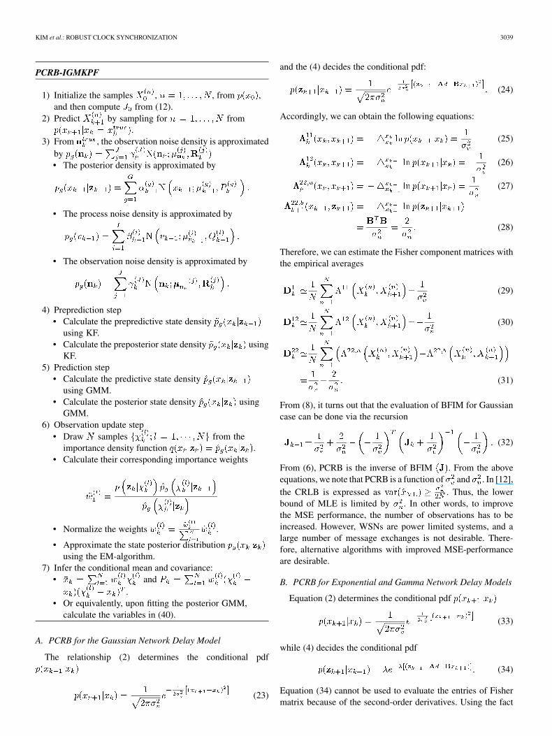
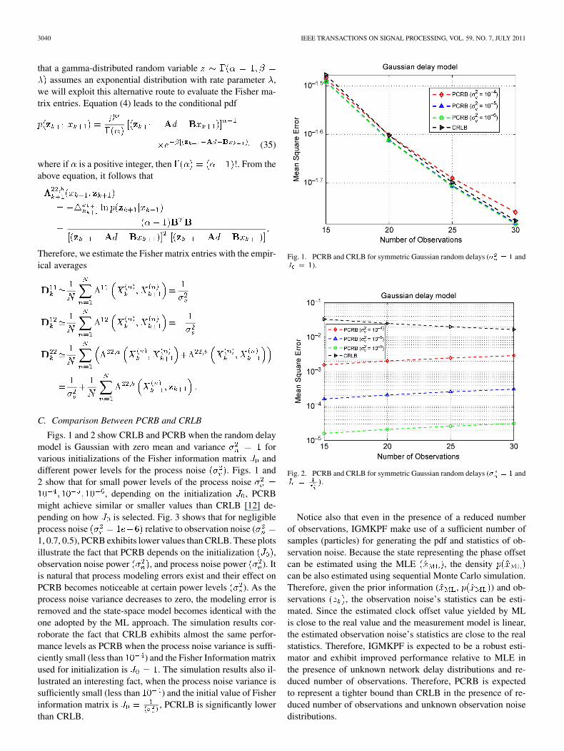
Figs. 1 and 2 show CRLB and PCRB when the random delaymodel is Gaussian with zero mean and variance forvarious initializations of the Fisher information matrix anddifferent power levels for the process noise . Figs. 1 and2 show that for small power levels of the process noise

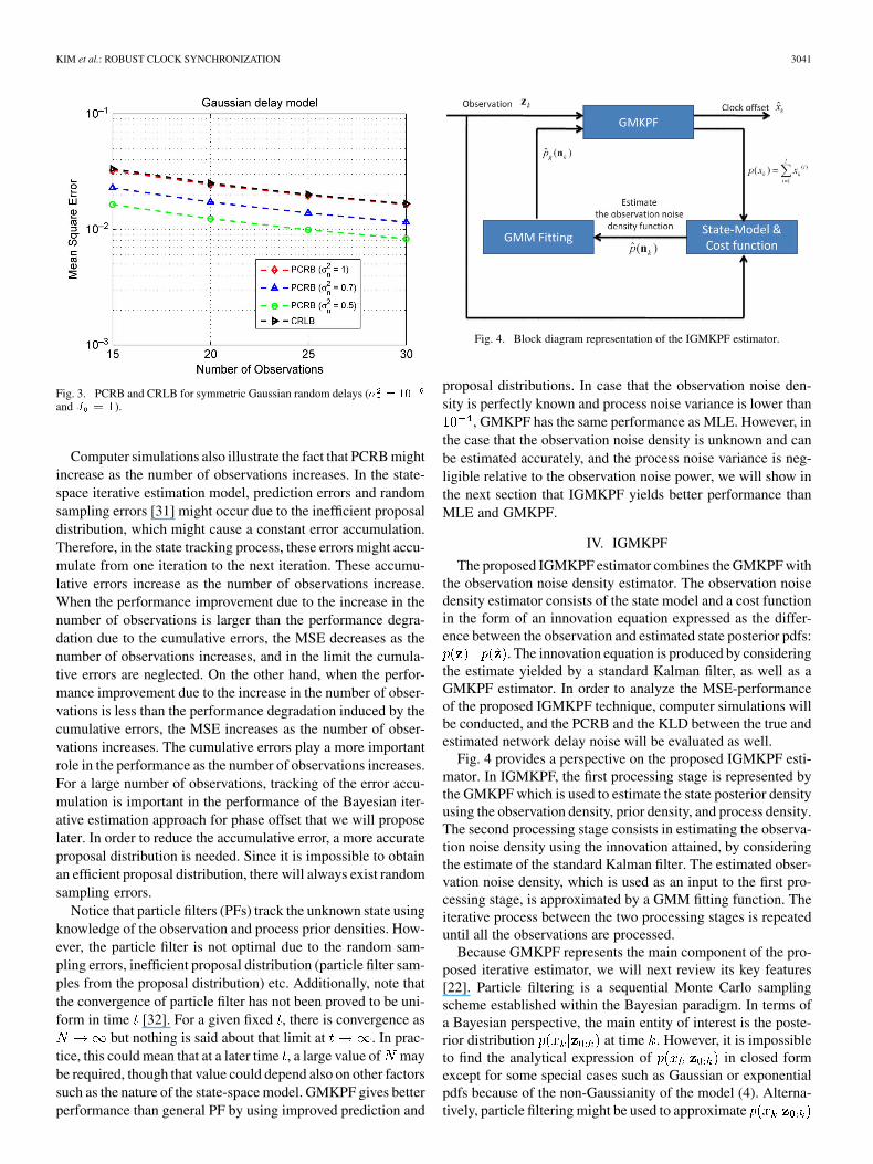
, depending on the initialization , PCRBmight achieve similar or smaller values than CRLB [12] de-pending on how is selected. Fig. 3 shows that for negligibleprocess noise relative to observation noise (1, 0.7, 0.5), PCRB exhibits lower values than CRLB. These plotsillustrate the fact that PCRB depends on the initialization ,observation noise power , and process noise power ). Itis natural that process modeling errors exist and their effect onPCRB becomes noticeable at certain power levels ). As theprocess noise variance decreases to zero, the modeling error isremoved and the state-space model becomes identical with theone adopted by the ML approach. The simulation results cor-roborate the fact that CRLB exhibits almost the same perfor-mance levels as PCRB when the process noise variance is suffi-ciently small (less than ) and the Fisher Information matrixused for initialization is . The simulation results also il-lustrated an interesting fact, when the process noise variance issufficiently small (less than ) and the initial value of Fisherinformation matrix is , PCRLB is significantly lowerthan CRLB.

Fig. 1. PCRB and CRLB for symmetric Gaussian random delays (� � � and� � �).

Fig. 2. PCRB and CRLB for symmetric Gaussian random delays (� � � and� � �.

Notice also that even in the presence of a reduced numberof observations, IGMKPF make use of a sufficient number ofsamples (particles) for generating the pdf and statistics of ob-servation noise. Because the state representing the phase offsetcan be estimated using the MLE , the densitycan be also estimated using sequential Monte Carlo simulation.Therefore, given the prior information ( , ) and ob-servations , the observation noise’s statistics can be esti-mated. Since the estimated clock offset value yielded by MLis close to the real value and the measurement model is linear,the estimated observation noise’s statistics are close to the realstatistics. Therefore, IGMKPF is expected to be a robust esti-mator and exhibit improved performance relative to MLE inthe presence of unknown network delay distributions and re-duced number of observations. Therefore, PCRB is expectedto represent a tighter bound than CRLB in the presence of re-duced number of observations and unknown observation noisedistributions.

KIM et al.: ROBUST CLOCK SYNCHRONIZATION 3041

Fig. 3. PCRB and CRLB for symmetric Gaussian random delays (� � ��

and � � �).

Computer simulations also illustrate the fact that PCRB mightincrease as the number of observations increases. In the state-space iterative estimation model, prediction errors and randomsampling errors [31] might occur due to the inefficient proposaldistribution, which might cause a constant error accumulation.Therefore, in the state tracking process, these errors might accu-mulate from one iteration to the next iteration. These accumu-lative errors increase as the number of observations increase.When the performance improvement due to the increase in thenumber of observations is larger than the performance degra-dation due to the cumulative errors, the MSE decreases as thenumber of observations increases, and in the limit the cumula-tive errors are neglected. On the other hand, when the perfor-mance improvement due to the increase in the number of obser-vations is less than the performance degradation induced by thecumulative errors, the MSE increases as the number of obser-vations increases. The cumulative errors play a more importantrole in the performance as the number of observations increases.For a large number of observations, tracking of the error accu-mulation is important in the performance of the Bayesian iter-ative estimation approach for phase offset that we will proposelater. In order to reduce the accumulative error, a more accurateproposal distribution is needed. Since it is impossible to obtainan efficient proposal distribution, there will always exist randomsampling errors.

Notice that particle filters (PFs) track the unknown state usingknowledge of the observation and process prior densities. How-ever, the particle filter is not optimal due to the random sam-pling errors, inefficient proposal distribution (particle filter sam-ples from the proposal distribution) etc. Additionally, note thatthe convergence of particle filter has not been proved to be uni-form in time [32]. For a given fixed , there is convergence as

but nothing is said about that limit at . In prac-tice, this could mean that at a later time , a large value of maybe required, though that value could depend also on other factorssuch as the nature of the state-space model. GMKPF gives betterperformance than general PF by using improved prediction and

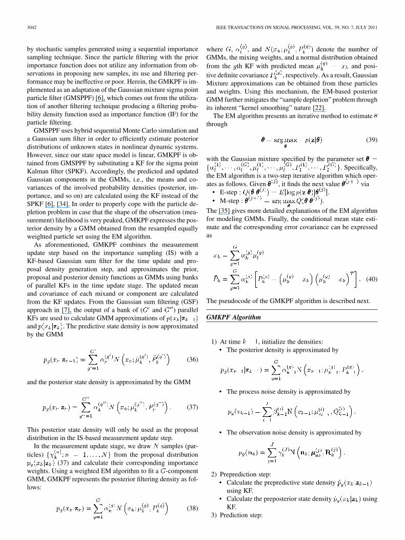
Fig. 4. Block diagram representation of the IGMKPF estimator.

proposal distributions. In case that the observation noise den-sity is perfectly known and process noise variance is lower than

, GMKPF has the same performance as MLE. However, inthe case that the observation noise density is unknown and canbe estimated accurately, and the process noise variance is neg-ligible relative to the observation noise power, we will show inthe next section that IGMKPF yields better performance thanMLE and GMKPF.

IV. IGMKPF

The proposed IGMKPF estimator combines the GMKPF withthe observation noise density estimator. The observation noisedensity estimator consists of the state model and a cost functionin the form of an innovation equation expressed as the differ-ence between the observation and estimated state posterior pdfs:

. The innovation equation is produced by consideringthe estimate yielded by a standard Kalman filter, as well as aGMKPF estimator. In order to analyze the MSE-performanceof the proposed IGMKPF technique, computer simulations willbe conducted, and the PCRB and the KLD between the true andestimated network delay noise will be evaluated as well.

Fig. 4 provides a perspective on the proposed IGMKPF esti-mator. In IGMKPF, the first processing stage is represented bythe GMKPF which is used to estimate the state posterior densityusing the observation density, prior density, and process density.The second processing stage consists in estimating the observa-tion noise density using the innovation attained, by consideringthe estimate of the standard Kalman filter. The estimated obser-vation noise density, which is used as an input to the first pro-cessing stage, is approximated by a GMM fitting function. Theiterative process between the two processing stages is repeateduntil all the observations are processed.

Because GMKPF represents the main component of the pro-posed iterative estimator, we will next review its key features[22]. Particle filtering is a sequential Monte Carlo samplingscheme established within the Bayesian paradigm. In terms ofa Bayesian perspective, the main entity of interest is the poste-rior distribution at time . However, it is impossibleto find the analytical expression of in closed formexcept for some special cases such as Gaussian or exponentialpdfs because of the non-Gaussianity of the model (4). Alterna-tively, particle filtering might be used to approximate

3042 IEEE TRANSACTIONS ON SIGNAL PROCESSING, VOL. 59, NO. 7, JULY 2011

by stochastic samples generated using a sequential importancesampling technique. Since the particle filtering with the priorimportance function does not utilize any information from ob-servations in proposing new samples, its use and filtering per-formance may be ineffective or poor. Herein, the GMKPF is im-plemented as an adaptation of the Gaussian mixture sigma pointparticle filter (GMSPPF) [6], which comes out from the utiliza-tion of another filtering technique producing a filtering proba-bility density function used as importance function (IF) for theparticle filtering.

GMSPPF uses hybrid sequential Monte Carlo simulation anda Gaussian sum filter in order to efficiently estimate posteriordistributions of unknown states in nonlinear dynamic systems.However, since our state space model is linear, GMKPF is ob-tained from GMSPPF by substituting a KF for the sigma pointKalman filter (SPKF). Accordingly, the predicted and updatedGaussian components in the GMMs, i.e., the means and co-variances of the involved probability densities (posterior, im-portance, and so on) are calculated using the KF instead of theSPKF [6], [34]. In order to properly cope with the particle de-pletion problem in case that the shape of the observation (mea-surement) likelihood is very peaked, GMKPF expresses the pos-terior density by a GMM obtained from the resampled equallyweighted particle set using the EM algorithm.

As aforementioned, GMKPF combines the measurementupdate step based on the importance sampling (IS) with aKF-based Gaussian sum filter for the time update and pro-posal density generation step, and approximates the prior,proposal and posterior density functions as GMMs using banksof parallel KFs in the time update stage. The updated meanand covariance of each mixand or component are calculatedfrom the KF updates. From the Gaussian sum filtering (GSF)approach in [7], the output of a bank of ( and ) parallelKFs are used to calculate GMM approximations ofand . The predictive state density is now approximatedby the GMM

(36)

and the posterior state density is approximated by the GMM

(37)

This posterior state density will only be used as the proposaldistribution in the IS-based measurement update step.

In the measurement update stage, we draw samples (par-ticles) from the proposal distribution

(37) and calculate their corresponding importanceweights. Using a weighted EM algorithm to fit a -componentGMM, GMKPF represents the posterior filtering density as fol-lows:

(38)

where , , and denote the number ofGMMs, the mixing weights, and a normal distribution obtainedfrom the th KF with predicted mean and posi-tive definite covariance , respectively. As a result, GaussianMixture approximations can be obtained from these particlesand weights. Using this mechanism, the EM-based posteriorGMM further mitigates the “sample depletion” problem throughits inherent “kernel smoothing” nature [22].

The EM algorithm presents an iterative method to estimatethrough

(39)

with the Gaussian mixture specified by the parameter set. Specifically,

the EM algorithm is a two-step iterative algorithm which oper-ates as follows. Given , it finds the next value via

• E-step : .• M-step : .

The [35] gives more detailed explanations of the EM algorithmfor modeling GMMs. Finally, the conditional mean state esti-mate and the corresponding error covariance can be expressedas

(40)

The pseudocode of the GMKPF algorithm is described next.

GMKPF Algorithm

1) At time , initialize the densities:• The posterior density is approximated by

• The process noise density is approximated by

• The observation noise density is approximated by

2) Preprediction step:• Calculate the prepredictive state density

using KF.• Calculate the preposterior state density using

KF.3) Prediction step:

KIM et al.: ROBUST CLOCK SYNCHRONIZATION 3043

• Calculate the predictive state densityusing GMM.

• Calculate the posterior state density usingGMM.

4) Observation Update step• Draw samples from the

importance density function .• Calculate their corresponding importance weights

• Normalize the weights .

• Approximate the state posterior distributionusing the EM-algorithm.

5) Infer the conditional mean and covariance• and

.• Or equivalently, upon fitting the posterior GMM,

calculate the variables in (40).

The improved performance of GMKPF comes with the priceof an increased computational complexity. Evaluating exactlythe number of floating point operations (flops) involved inGMKPF is not possible because it is an iterative and quite com-plex algorithm. However, we will evaluate its computationalcomplexity by quantifying only the most computationallydemanding steps in terms of the Big O notation. Letdenote the dimension of the state vector , and representby the number of particles (samples in pseudocode) andthrough the number of GMM components. The state vectorand matrices are , , , where

is the a posteriori error covariance matrix. The KalmanFilter requires approximately flops since the matrixtimes matrix multiplication is the most time consuming step

, whereas the particle filter assumesapproximately flops due to the matrix times vectormultiplication ( , ) and samplingstep. The GMKPF necessitates approximately flopsdue to the KF-step and flops due to the EM-step(considering only the most computationally demanding stepsand neglecting the rest of operations). If , GMKPF re-quires approximately flops. Notice also that MLEgnecessitates approximately flops because it involvessummations and a division. This indicates that GMKPF isapproximately 300 times slower than MLEg in an applicationwith , , and .

In IGMKPF, at the first iteration, GMKPF initializes thedensities and estimates the state posterior pdf using particlesfor generation of pdfs (posterior pdf, prior pdf, process noisepdf, observation noise pdf, and so on). Next, the observationnoise density generator block estimates the observation noisepdf using both the measurement observations and the posteriordensity computed by GMKPF. This iteration is repeated upto the number of observations. The pseudocode of IGMKPFalgorithm is next described.

IGMKPF Algorithm

1) At time , initialize the densities and set the initial state.

2) GMKPF step (estimate the state posterior density).• Calculate the state posterior density using

GMKPF.• If reaches the end of observations, go to “Infer the

conditional mean and covariance step.”3) Estimate the Observation Noise Density (OND) step

• Calculate the observation noise density givenand , and state model [(2) and (4)].

• The observation noise density using GMM isapproximated by

4) , go to the GMKPF step.5) Infer the conditional mean and covariance

• and

.• Or equivalently, upon fitting the posterior GMM,

calculate the variables in (40).

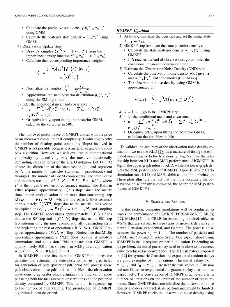
To validate the accuracy of the observation noise density es-timation, we use the KLD [28] as a measure of fitting the esti-mated noise density to the true density. Fig. 5 shows the rela-tionship between KLD and MSE-performance of IGMKPF. InFig. 5, the upper graph refers to KLD, while the lower graph de-picts the MSE performance of IGMKPF. Upon 10 Monte Carlosimulation runs, KLD and MSE exhibit a quite similar behavior.These plots illustrate the fact that the more accurately the ob-servation noise density is estimated, the better the MSE perfor-mance of IGMKPF is.

V. SIMULATION RESULTS

In this section, computer simulations will be conducted toassess the performance of IGMKPF, PCRB-IGMKPF, MLEg[12], MLEe [12], and CRLB for estimating the clock offset inWSNs that are subject to three types of network delays: sym-metric Gaussian, exponential, and Gamma. The process noiseassumes the power . The number of particles andGMMs are 500 and 3, respectively. One aspect about usingIGMKPF is that it requires proper initialization. Depending onthe problem, the initial guess may need to be close to the correctvalue to achieve fast convergence. The ML estimators proposedin [12] for symmetric Gaussian and exponential random delaysare good examples of initializations. The initial values

, and are near the true values in Gaussianand non-Gaussian (exponential and gamma) delay distributions,respectively. The convergence of IGMKPF is achieved after anumber of iterations on the order of the number of measure-ments. Since GMKPF does not initialize the observation noisedensity and does not track it, its performance might be limited.However, IGMKPF tracks the observation noise density using

3044 IEEE TRANSACTIONS ON SIGNAL PROCESSING, VOL. 59, NO. 7, JULY 2011

Fig. 5. KLD and MSE for symmetric exponential random delays �� � ��.

the observation and estimated posterior pdfs. Therefore, the per-formance of IGMKPF is expected to be better than GMKPF andMLE.

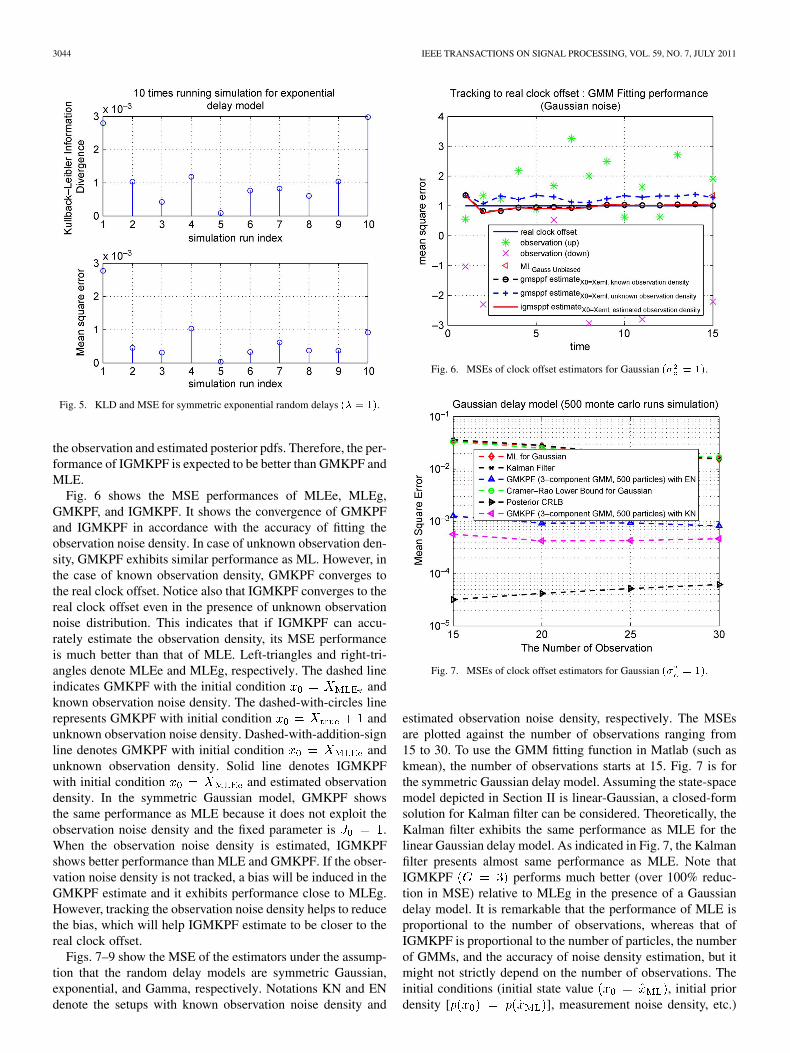
Fig. 6 shows the MSE performances of MLEe, MLEg,GMKPF, and IGMKPF. It shows the convergence of GMKPFand IGMKPF in accordance with the accuracy of fitting theobservation noise density. In case of unknown observation den-sity, GMKPF exhibits similar performance as ML. However, inthe case of known observation density, GMKPF converges tothe real clock offset. Notice also that IGMKPF converges to thereal clock offset even in the presence of unknown observationnoise distribution. This indicates that if IGMKPF can accu-rately estimate the observation density, its MSE performanceis much better than that of MLE. Left-triangles and right-tri-angles denote MLEe and MLEg, respectively. The dashed lineindicates GMKPF with the initial condition andknown observation noise density. The dashed-with-circles linerepresents GMKPF with initial condition andunknown observation noise density. Dashed-with-addition-signline denotes GMKPF with initial condition andunknown observation density. Solid line denotes IGMKPFwith initial condition and estimated observationdensity. In the symmetric Gaussian model, GMKPF showsthe same performance as MLE because it does not exploit theobservation noise density and the fixed parameter is .When the observation noise density is estimated, IGMKPFshows better performance than MLE and GMKPF. If the obser-vation noise density is not tracked, a bias will be induced in theGMKPF estimate and it exhibits performance close to MLEg.However, tracking the observation noise density helps to reducethe bias, which will help IGMKPF estimate to be closer to thereal clock offset.

Figs. 7–9 show the MSE of the estimators under the assump-tion that the random delay models are symmetric Gaussian,exponential, and Gamma, respectively. Notations KN and ENdenote the setups with known observation noise density and

Fig. 6. MSEs of clock offset estimators for Gaussian �� � ��.

Fig. 7. MSEs of clock offset estimators for Gaussian �� � ��.

estimated observation noise density, respectively. The MSEsare plotted against the number of observations ranging from15 to 30. To use the GMM fitting function in Matlab (such askmean), the number of observations starts at 15. Fig. 7 is forthe symmetric Gaussian delay model. Assuming the state-spacemodel depicted in Section II is linear-Gaussian, a closed-formsolution for Kalman filter can be considered. Theoretically, theKalman filter exhibits the same performance as MLE for thelinear Gaussian delay model. As indicated in Fig. 7, the Kalmanfilter presents almost same performance as MLE. Note thatIGMKPF performs much better (over 100% reduc-tion in MSE) relative to MLEg in the presence of a Gaussiandelay model. It is remarkable that the performance of MLE isproportional to the number of observations, whereas that ofIGMKPF is proportional to the number of particles, the numberof GMMs, and the accuracy of noise density estimation, but itmight not strictly depend on the number of observations. Theinitial conditions (initial state value , initial priordensity [ ], measurement noise density, etc.)

KIM et al.: ROBUST CLOCK SYNCHRONIZATION 3045

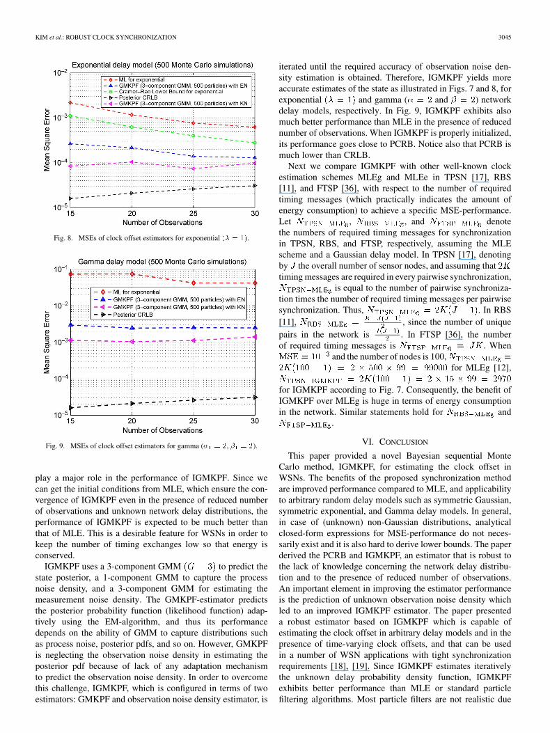
Fig. 8. MSEs of clock offset estimators for exponential �� � ��.

Fig. 9. MSEs of clock offset estimators for gamma (� � �, � � �).

play a major role in the performance of IGMKPF. Since wecan get the initial conditions from MLE, which ensure the con-vergence of IGMKPF even in the presence of reduced numberof observations and unknown network delay distributions, theperformance of IGMKPF is expected to be much better thanthat of MLE. This is a desirable feature for WSNs in order tokeep the number of timing exchanges low so that energy isconserved.

IGMKPF uses a 3-component GMM to predict thestate posterior, a 1-component GMM to capture the processnoise density, and a 3-component GMM for estimating themeasurement noise density. The GMKPF-estimator predictsthe posterior probability function (likelihood function) adap-tively using the EM-algorithm, and thus its performancedepends on the ability of GMM to capture distributions suchas process noise, posterior pdfs, and so on. However, GMKPFis neglecting the observation noise density in estimating theposterior pdf because of lack of any adaptation mechanismto predict the observation noise density. In order to overcomethis challenge, IGMKPF, which is configured in terms of twoestimators: GMKPF and observation noise density estimator, is

iterated until the required accuracy of observation noise den-sity estimation is obtained. Therefore, IGMKPF yields moreaccurate estimates of the state as illustrated in Figs. 7 and 8, forexponential and gamma ( and ) networkdelay models, respectively. In Fig. 9, IGMKPF exhibits alsomuch better performance than MLE in the presence of reducednumber of observations. When IGMKPF is properly initialized,its performance goes close to PCRB. Notice also that PCRB ismuch lower than CRLB.

Next we compare IGMKPF with other well-known clockestimation schemes MLEg and MLEe in TPSN [17], RBS[11], and FTSP [36], with respect to the number of requiredtiming messages (which practically indicates the amount ofenergy consumption) to achieve a specific MSE-performance.Let , , and denotethe numbers of required timing messages for synchronizationin TPSN, RBS, and FTSP, respectively, assuming the MLEscheme and a Gaussian delay model. In TPSN [17], denotingby the overall number of sensor nodes, and assuming thattiming messages are required in every pairwise synchronization,

is equal to the number of pairwise synchroniza-tion times the number of required timing messages per pairwisesynchronization. Thus, . In RBS[11], , since the number of uniquepairs in the network is . In FTSP [36], the numberof required timing messages is . When

and the number of nodes is 100,for MLEg [12],

for IGMKPF according to Fig. 7. Consequently, the benefit ofIGMKPF over MLEg is huge in terms of energy consumptionin the network. Similar statements hold for and

.

VI. CONCLUSION

This paper provided a novel Bayesian sequential MonteCarlo method, IGMKPF, for estimating the clock offset inWSNs. The benefits of the proposed synchronization methodare improved performance compared to MLE, and applicabilityto arbitrary random delay models such as symmetric Gaussian,symmetric exponential, and Gamma delay models. In general,in case of (unknown) non-Gaussian distributions, analyticalclosed-form expressions for MSE-performance do not neces-sarily exist and it is also hard to derive lower bounds. The paperderived the PCRB and IGMKPF, an estimator that is robust tothe lack of knowledge concerning the network delay distribu-tion and to the presence of reduced number of observations.An important element in improving the estimator performanceis the prediction of unknown observation noise density whichled to an improved IGMKPF estimator. The paper presenteda robust estimator based on IGMKPF which is capable ofestimating the clock offset in arbitrary delay models and in thepresence of time-varying clock offsets, and that can be usedin a number of WSN applications with tight synchronizationrequirements [18], [19]. Since IGMKPF estimates iterativelythe unknown delay probability density function, IGMKPFexhibits better performance than MLE or standard particlefiltering algorithms. Most particle filters are not realistic due

3046 IEEE TRANSACTIONS ON SIGNAL PROCESSING, VOL. 59, NO. 7, JULY 2011

to many assumptions (including a-priori knowledge of obser-vation noise distribution). PCRB represents a lower bound forthe MSE performance of IGMKPF. Because of the difficulty inevaluating PCRB in closed-form expression, the plotted PCRBgraphs represent simulated bounds (obtained via IGMKPF) ofthe actual PCRB. In the presence of optimal settings (efficientproposal, optimal number of particles, etc.), the simulatedPCRB might represent a tighter bound. The performance gapbetween IGMKPF and PCRB is due to the impossibility of es-timating precisely the observation noise density with a reducednumber of observations. There are also the sampling errors,the error accumulation due to the iterative nature of algorithmand inefficient proposal distribution that contribute to this. Theproposed clock synchronization algorithm considers only thecorrection of clock phase-offset errors. Extension of this workto the situation when clock skew and drift errors are presentrepresents an interesting open research problem.

REFERENCES

[1] F. Sivrikaya and B. Yener, “Time synchronization in sensor networks:A survey,” IEEE Netw., pp. 45–50, Jul./Aug. 2004.

[2] B. Sadler, “Critical issues in energy-constrained sensor networks:Synchronization, scheduling, and acquisition,” in Proc. ICASSP 2005,2005, vol. 5, pp. 785–788.

[3] B. Sadler and A. Swami, “Synchronization in sensor networks: Anoverview,” in Proc. MILCOM 2006, Wash. DC, 2006, pp. 1–6.

[4] B. Sundararaman, U. Buy, and A. D. Kshemkalyani, “Clock synchro-nization for wireless sensor networks: A survey,” Ad Hoc Netw., vol. 3,no. 3, pp. 281–323, May 2005.

[5] B. D. Anderson and J. B. Moore, Optimal Filtering. EnglewoodCliffs, NJ: Prentice-Hall, 1979.

[6] R. van der Merwe and E. Wan, “Gaussian mixture sigma-point par-ticle filters for sequential probabilistic inference in dynamic state-spacemodels,” in Proc. Int. Conf. Acoust., Speech, Signal Process. (ICASSP),Apr. 2003.

[7] O. L. Alspach and H. W. Sorenson, “Nonlinear Bayesian estimationusing Gaussian sum approximation,” IEEE Trans. Autom. Control, vol.17, no. 4, pp. 439–448, 1972.

[8] G. J. Pottie and W. J. Kaiser, “Wireless integrated network sensors,”Commun. ACM, vol. 43, no. 5, pp. 51–58, May 2000, 0001-0782.

[9] I. Akyildiz et al., “Wireless sensor networks: A survey,” Comput. Netw., vol. 38, no. 4, pp. 393–422, Mar. 2002.

[10] H. S. Abdel-Ghaffar, “Analysis of synchronization algorithm withtime-out control over networks with exponentially symmetric delays,”IEEE Trans. Commun., vol. 50, no. 10, pp. 1652–1661, Oct. 2002.

[11] J. Elson, L. Girod, and D. Estrin, “Fine-grained network time synchro-nization using reference broadcasts,” in Proc. 5th Symp. Operat. Syst.Design Implement. (OSDI 2002), Dec. 2002.

[12] K.-L. Noh, Q. M. Chaudhari, E. Serpedin, and B. W. Suter, “Novelclock phase offset and skew estimation using two-way timing messageexchanges for wireless sensor networks,” IEEE Trans. Commun., vol.55, no. 4, Apr. 2007.

[13] M. Leng and Y.-C. Wu, “On clock synchronization Algorithms forwireless sensor networks under unknown delay,” IEEE Trans. Veh.Technol., vol. 59, no. 1, pp. 182–190, Jan. 2010.

[14] D. Mills, “Internet time synchronization: The network time protocol(NTP),” IEEE Trans. Commun., vol. 39, pp. 1482–1493, 1991.

[15] K. Noh, E. Serpedin, and K. Qaraqe, “A new approach for time syn-chronization in wireless sensor networks: Pairwise Broadcast Synchro-nization (PBS),” IEEE Trans. Wireless Commun., vol. 7, no. 6, Sep.2008.

[16] I. Skog and P. Handel, “Synchronization by two-way message ex-changes: Cramer-Rao bounds, approximate maximum likelihood, andoffshore submarine positioning,” IEEE Trans. Signal Process., vol. 58,no. 4, pp. 2351–2362, Apr. 2010.

[17] S. Ganeriwal, R. Kumar, M. B., and Srivastava , “Timing-sync protocolfor sensor networks,” in Proc. 1st Int. Conf. Embedded Network Sens.Syst. , 2003, pp. 138–149, ACM.

[18] J. Heidemann, W. Ye, J. Wills, A. Syed, and Y. Li, “Research chal-lenges and applications for underwater sensor networking,” in Proc.IEEE Wireless Commun. Netw. Conf., Apr. 2006, vol. 1, pp. 228–235.

[19] A. Syed and J. Heidemann, “Time synchronization for high latencyacoustic networks,” USC/Inf. Sci. Inst., Tech. Rep. ISI-TR-2005-602,Apr. 2005.

[20] E. L. Lehmann and G. Casella, Theory of Point Estimation, 2nd ed.New York: Springer, 1998.

[21] H. L. Van Trees, Detection, Estimation, and Modulation Theory. NewYork: Wiley, 1968, vol. 1.

[22] J. Kim, J. Lee, E. Serpedin, and K. Qaraqe, “A robust estimationscheme for clock phase offsets in wireless sensor networks in thepresence of non-Gaussian random delays,” Signal Process., pp.1155–1161, 2009.

[23] F. Kirsch and M. Vossiek, “Distributed Kalman filter for precise androbust clock synchronization in wireless networks,” in Proc. 4th Int.Conf. Radio and Wireless Symp., San Diego, CA, 2009, pp. 455–458.

[24] B. R. Hamilton, X. Ma, Q. Xhao, and J. Xu, “ACES: Adaptive clockestimation and synchronization using Kalman filtering,” in Proc. 14thACM Int. Conf. Mobile Comput. Netw., San Francisco, CA, 2008, pp.152–162.

[25] S. Ganeriwal, D. Ganesan, H. Shim, V. Tsiatsis, and M. B. Srivastava,“Estimating clock uncertainty for efficient duty-cycling in sensor net-works,” in ACM Sensys Conf., San Diego, CA, Nov. 2005, pp. 130–141.

[26] Q. Gao, K. J. Blow, and D. J. Holding, “Simple algorithm for improvingtime synchronization in wireless sensor networks,” Electron. Lett., vol.40, p. 889, 2004.

[27] D. Tulone, “Resource-efficient time synchronization for wirelesssensor networks,” in Proc. DIALM-POMC Workshop Found. MobileComput., Philadelphia, PA, Oct. 2004, p. 52-50.

[28] S. Kullback, Information Theory and Statistics. Mineola, NY: Dover,1968.

[29] J. Hershey and P. A. Olsen, “Approximating the Kullback-Leiblerdivergence between Gaussian mixture models,” in Proc. IEEE Int.Conf. Acoust., Speech Signal Process. (ICASSP 2007), 2007, vol. 4,pp. 317–320.

[30] P. Tichavsky, C. Muravchik, and A. Nehorai, “Posterior Cramer-Raobounds for discrete-time nonlinear filtering,” IEEE Trans. SignalProcess., vol. 46, no. 5, May 1998.

[31] A. Doucet, N. de Freitas, and N. Gordon, Sequential Monte CarloMethods in Practice. New York: Springer-Verlag, 2001.

[32] M. Isard and A. Blake, “Condensation-conditional density propagationfor visual tracking,” Int. J. Comput. Vision, vol. 29, no. 1, pp. 5–28,1998.

[33] H. Elders-Boll, H.-D. Schotten, and A. Busboom, “Efficient implemen-tation of linear multiuser detectors for asynchronous CDMA systemsby linear interference cancellation,” Eur. Trans. Telecommun., vol. 9,no. 5, pp. 427–438, May 1998.

[34] S. Julier and J. K. Uhlmann, “A general method for approximating non-linear transformations of probability distributions,” Robot. Res. Group,Dep. Eng. Sci., Univ. Oxford, Oxford, U.K., Tech. Rep., 1996.

[35] F. Pernkopf and D. Bouchaffra, “Genetic-based EM algorithm forlearning Gaussian mixture models,” IEEE Trans. Pattern Anal. Mach.Intell., vol. 27, no. 8, Aug. 2005.

[36] M. Maroti, B. Kusy, G. Simon, and A. Ledeczi, “The flooding time syn-chronization protocol,” in Proc. 2nd Int. Conf. Embedded Netw. Sens.Syst. 2004, Nov. 2004, pp. 39–49, ACM Press.

Jang-Sub Kim was born June 15, 1974, inYeongdeok, Korea. He received the M.S. and Ph.D.degrees from the School of Electrical and ComputerEngineering, Sungkyunkwan University, Seoul,Korea, in 1999 and 2005, respectively.

He is currently a Visiting Researcher with theDepartment of Electrical and Computer Engi-neering, Texas A&M University, College Station.His research interests include signal processing andits applications in wireless communications andnetworking, synchronization for wireless sensor

networks and wireless communications, and sequential Monte Carlo methods.

KIM et al.: ROBUST CLOCK SYNCHRONIZATION 3047

Jaehan Lee received the B.S. degree and the M.S.degree in electrical engineering from Seoul NationalUniversity, Korea, in 1997 and 1999, respectively. Hereceived the Ph.D. degree in electrical engineeringfrom Texas A&M University, College Station, in2010.

Since then, he has been working as a principalengineer for Samsung SDS in Seoul, Korea. Hisresearch interests include clock synchronization inWSNs, Internet of Things (IoT), Web of Things(WoT), and M2M communications.

Erchin Serpedin received the specialization degreein signal processing and transmission of informationfrom Ecole Superieure D’Electricite (SUPELEC),Paris, France, in 1992, the M.Sc. degree from theGeorgia Institute of Technology, Atlanta, in 1992,and the Ph.D. degree in electrical engineering fromthe University of Virginia, Charlottesville, in January1999.

In July 1999, he joined Texas A&M University,College Station, where he currently holds the positionof Professor. His research interests lie in the areas of

signal processing, telecommunications, bioinformatics, and genomics. He is theauthor of 70 journal papers and 100 conference papers, and coauthor of the re-search monograph Synchronization in Wireless Sensor Networks (Cambridge,U.K.: Cambridge University Press, August 2009).

Dr. Serpedin received the NSF Career Award in 2001, the Outstanding Fac-ulty Award in 2004, and several other awards. He served as an Associate Editorfor the IEEE COMMUNICATIONS LETTERS, IEEE TRANSACTIONS ON SIGNAL

PROCESSING, IEEE SIGNAL PROCESSING LETTERS, IEEE TRANSACTIONS ON

WIRELESS COMMUNICATIONS, and EURASIP Journal on Advances in SignalProcessing. He served as a Technical Co-Chair of the Communications TheorySymposium at Globecom 2006 Conference, and for the VTC Fall 2006:Wireless Access Track Symposium. He is currently serving as AssociateEditor for the journals Signal Processing- Elsevier, the IEEE TRANSACTIONS

ON COMMUNICATIONS, IEEE TRANSACTIONS ON INFORMATION THEORY,EURASIP Journal on Advances in Signal Processing, and EURASIP Journalon Bioinformatics and Systems Biology.

Khalid Qaraqe (M’97–SM’00) was born inBethlehem. He received the B.S. degree from theUniversity of Technology, Baghdad, in 1986, withhonors, the M.S. degree from the University ofJordan, Jordan, in 1989, and the Ph.D. degree fromTexas A&M University, College Station, in 1997, allin electrical engineering.

From 1989 to 2004, he held a variety of positionsin many companies. He has more than 12 years of ex-perience in the telecommunication industry. He hasworked for Qualcomm, Enad Design Systems, Ca-

dence Design Systems/Tality Corporation, STC, SBC, and Ericsson. He has alsoworked on numerous GSM, CDMA, WCDMA projects and has experience inproduct development, design, deployment, testing, and integration. He joinedthe Department of Electrical Engineering, Texas A&M University at Qatar, inJuly 2004, where he is now an Associate Professor. His research interests in-clude communication theory and its application to design and performance anal-ysis of cellular systems and indoor communication systems. Particular interestsare in the development of 3G UMTS, cognitive radio systems, broadband wire-less communications, and diversity techniques.