The detection and estimation of long memory in stochastic volatility

ELSEVIER Journal of Econometrics 83 (1998) 325-348

JOURNAL OF Econometrics

The detection and estimation of long memory in stochastic volatility

F. J a y Bre id t a, N u n o Cra to b, P e d r o de L i m a ¢'*

aDepartment of Statistics, Iowa State University, Ames, IA 50011, USA b Department t~" Mathematics. New Jersey Institute of Technology, NJ 07102, USA

C Department ~" Economics, The Johns Hopk#~s Unirersity, Bait#note, MD 21218, USA

Received ! March 1995; received in revised form ! March 1996

Abstract

We propose a new time series representation of persistence in conditional variance called a long memory stochastic volatility (LMSV) model. The LMSV model is constructed by incorporating an ARFIMA process in a standard stochastic volatility scheme. Strongly consistent estimators of the parameters of the model are obtained by maximizing the spectral approximation to the Gaussian likelihood. The finite sample properties of the spectral likelihood estimator are analyzed by means of a Monte Carlo study. An empirical example with a long time series of stock prices demonstrates the superiority of the LMSV model over existing (short-memory) volatility models, ~ 1998 Elsevier Science S.A.

Key u'ords: Fractional ARMA; EGARCII; Spectral likelihood estimators JEL chtss(lication." C22

I. introduction

A large body o f research suggests that the conditional volatility o f asset prices

displays long memory or long-range persistence. I Furthermore, as we demonstra te

below, this type of persistence cannot be appropriately modeled by autoregressive

* Corresponding author. This paper was presented at a conference in honor of Carl Christ held at the Johns Hopkins

University in April 1995. We are thankful to our discussant Patrick Asea, seminar participants at the University of Pennsylvania, Francis Diebold, Thomas Epps, and two anonymous referees for helpful comments. Any remaining errors are our own.

I See Ding et al. (1993), de Lima and Crato (1993) and Bollerslev and Mikkelsen (1996) for evidence that persistence in stock markets' volatility can be characterized as a long memory process.

0304-4076/98/$19.00 (~ 1998 Elsevier Science S.A. All rights reserved PII S 0 3 0 4 - 4 0 7 6 ( 9 7 ) 0 0 0 7 2 - 9

326 F. Jay Breidt et al./Journal of Econometrh's 83 (1998) 325-348

conditional heteroskedastic (ARCH), generalized ARCH (GARCH), exponential GARCH (EGARCH) or standard (short-memory) stochastic volatility models. 2

In light of these recent findings and the limitations of short-memory models of stochastic volatility in this paper we propose a new time series representation of persistence in conditional volatility that we call a long memory stochastic volatility model (LMSV). 3 The LMSV model is constructed by incorporating an ARFIMA process in a standard stochastic volatility scheme. We show that the parameters of the LMSV models can be estimated by applying a frequency domain likelihood estimator. 4 The finite sample properties of the spectral likelihood estimator are evaluated by means of a Monte Carlo study.

The LMSV model has several advantages. First, because it is well-defined in the mean square sense many of its stochastic features are easy to establish. Second, because it has well-known counterparts in models for level series it inherits most of the statistical properties of those models.

The rest of the paper proceeds as follows. In Section 2 we review models of persistence in volatility (i.e. fractional GARCH and EGARCH models) and introduce the long-memory stochastic volatility model. In Section 3 we present further empirical evidence on the relevance of long memory by testing the null of short memory, for proxies of the conditional variances in an extensive set of US stock return indexes. In Section 4 we discuss a Whittle-type estimator for the LMSV model parameters obtained by maximizing the spectral approximation to the Gaussian likelihood. We present finite-sample simulation evidence about the properties of the estimators and, as an example, we study the daily returns for the value-weighted CRSP market index, in Section 5 we conclude. Proofs are Ibund in the appendicc~,~;.

Z. Models of persistence in volatility

Following Brockwell and Davis, (1991) we state that a weakly stationary process has short memory when its autocorrelation function (ACF), say p(h), is geometrically bounded

[p(h)[ ~< Cr II~1 for some C > 0, 0 < r < 1.

in contrast to a short-memory process with a geometrically decaying ACF, a weakly stationary process has long memory if its ACF p(.) has a hyperbolic

~' See Bollerslev et al. (1992) tbr a review of ARCtt and GARCll-type models, and Taylor (1994) tbr a recent review of stochastic volatility models.

~ Harvey (1993) independently proposed a stochastic volatility model driven by fractional noise and applied it to exchange rate series, obtaining smoothed estimates of the underlying volatilities.

4 This work was directly motivated by the empirical results of de Lima and Crato (1993).

F. Jay Breidt et al. I Journal of Econometrics 83 (1998) 325-348 327

decay,

p(h) , ' , , Ch 2d- I as h ~ c~,

where C # 0 and d <0.5 (e.g., Brockwell and Davis, 1991, Section 13.2). Alter- natively, we can say the process has long memory if its spectrum f ( 2 ) has the asymptotic decay

f (2 ) ~ C[21-2a as 2 4 0 with d #0 . (1)

If, in addition, d > 0 , then the autocorrelations are not absolutely summable, Ip(h)l =oo, and the spectrum diverges at zero, f (2 )T c¢ as 2 4 0 . In this

case we conclude that the process is persistent. For a discussion of alternative long-memory characterizations see Sections 2.2 and 2.3 of Baillie (1996).

2.1. GARCH and EGARCH models

Following Engle (1982), Bollerslev (1986) and Nelson (1991), let the predic- tion error y, satisfy

yt =ate,,

where { ~t } is independent and identically distributed (i.i.d.) with mean zero and variance one, and tr~ is the variance of yt given information at time t - 1. Among the most successful specifications for the conditional variance a~ are the GARCH and EGARCtt models. A GARCH specification is given by

q p ~ ,,2 (2)

where to > 0. Constraints on {hi } anti {aj } are discussed below. More compactly, we can write Eq. (2) as

h(B)a = + . ( 8 ) f i ,

where B is the backshift operator (Bivt=vt_j, j = 0 , : h l , + 2 , . . . ) , b(z)= 1 - b l z . . . . . bqZ q and a(z)=alz + . . . + apZ p.

As an alternative to the GARCH specification, Nelson (1991) proposes the Exponential GARCH (EGARCH) model

o o

log ,r, 2 = + E ,) , - !, (3 ) j=0

where no restriction is needed for the signs of the coefficients. The function g(.) may be chosen to allow for asymmetric changes, depending on the sign of ~t.

It is known that the GARCH model (Bollerslev, 1986) can also be written in an ARMA(max { p, q}, q) form, with the process { y2 } being driven by the noise

328 F Jay Breidt et aL/Journal of Econometrics 83 (1998) 325-348

vt = y2 _ 0.2. From this representation it is clear that the autocorrelation function for {yt 2 } has a short-memory geometric decay.

EGARCH models have the general representation as in (3), but they are also usually parameterized with weights { qtj } corresponding to an ARMA(p, q). Thus, the usual EGARCH specification can be written as:

~b(B)(log a2 _ i t , ) = O(B)ff(~t_y_l ),

where q~(z) = 1 - ~plz . . . . . dppz p ~ 0 for Izl ~< 1 is an autoregressive polynomial, 0(z)= 1 +Olz + . . . + O q z q is a moving average polynomial and O(z) has no roots in common with tp(z).

The empirical evidence previously discussed points in the direction of long memory, both in the squared process {yt 2 } and in the process of log squares {log y2}. This contrasts with the usual short-memory formulations of GARCH and EGARCH models. We will look for the formulation of models with persistent properties.

2.2. Long-memory G A R C H models

In order to accommodate the findings of long memory, a sensible approach is to generalize GARCH models by using fractional differences, along lines ear- lier suggested by Robinson (1991, p. 82). The fractional differencing operator is defined through the expansion

r(j - d ) (i - B)d= ~ )B J,

• /~o F ( j + I ) F ( - d

from which Baillie et al. (1996) tbrmulated the fractionally integrated GARCH (FIGARCH) model

( I - a)'q)(B)(~ - t~) = a(B)(y, 2 - ~).

Baillie et al. (1996) suggested quasi-maximum-likelihood estimation methods for this model.

In order to have a well-defined process, the parameters {aj }, {bj }, and d are constrained so that the coefficients ~j in the representation

#," = u + ( ! - a ) - ' ~ a ( a ) b - ' ( a ) y , - = l~ + ~ ¢, j ty~_~_/ j=O

- l~), (4)

are all nonnegative. Otherwise we have af <0 with a positive probability. This implies that the parameters {a i } and {bj } are constrained as in the standard GARCH models. This also implies that the parameter d is constrained to be positive, and so ~]j~0 ~J = ~x~. However, this means that the sum of all coefficients is greater than one. It follows fi'om a now standard result in Bollerslev (1986) that {yt } is not covariance stationary. Consequently, the autocovariance function

F. Jay Breidt et al./Journal of Econometrics 83 (1998) 325-348 329

(ACVF) of the process {yt 2 } is not defined, s the series Y]~j=0 ~'Jt.}'LI-j - #)

is not defined in L 2, and the use of spectral and time-domain autocorrelation methods is not justifiable in a standard way. In addition, initializing the quasi- likelihood, which is usually done with unconditional moments of out-of-sample trt 2, can be problematical, although Baillie et al. (1996) reported good results for the quasi-maximum-likelihood estimation method.

As an alternative, Nelson (1991, p. 352) notes that persistence can be modeled in the log squares with a long-memory specification of an EGARCH model. Bollerslev and Mikkelsen (1996) have explicitly formulated a fractionally integrated EGARCH model of the form

loga 2 =,ut + O(B)~b(B)-I(I - B)-dg(¢t_~), (5)

where ~(z) and O(z) are defined above. This generalization of EGARCH with fractional noise gives a strictly stationary and ergodic process. The condition for the covariance stationarity of {logat z - #t} is Y~'~j~0 ~bi z <1 (Theorem 2.1 of

i Nelson, 1991 ), which is satisfied for a parameter value d < i. EGARCH models have the convenient feature that the coefficients in the mov-

ing average expansion (5) are not restricted to be positive. However, asymptotic results about the estimators have proven to be extremely hard to obtain, even when d = 0.

2.3. A long memory stochastic volatility model

In this subsection we introduce a different approach, based on stochastic volatility (SV) models similar to those discussed by Melino aad Turnbull (1990) and Harvey et al. (1994).

The stochastic volatility model is defined by

3'~ =ate.t, at =aexp(vd2), (6)

where {v,} is independent of {~., }, {~, } is independent and identically distributed (i.i.d.) with mean zero and variance one, and { vt } is an ARMA model.

The long memory stochastic volatility (LMSV) model we now introduce is defined by (6) with { vt } being a stationary long-memory process.

Restricting our attention to a Gaussian {vt }, it follows that {yt } is both covariance and strictly stationary. Denote by 7(') the ACVF of {vt }. The covariance structure of )'1 is obtained from properties of th,. • Iognormal distribution:

E[yt]=0, Var(yt)= exp{7(0)/2}a 2 and

Cov(.vt, y, +h ) = 0 for h ~ O,

5 However, this model displays the important property of having a bounded cumulative impulse- response function tbr any d < l as Baillie et al. (1996)have shown.

330 F. Jay Breidt et al./Journal of Econometrics 83 (1998) 325-348

so that {Yt } is a white noise sequence. In fact, {Y t} is a martingale difference, a property inherited from {~t }. An appealing property of this model in terms of its empirical relevance is the excess kurtosis displayed by yt, which is

E[y 4] 3 = 3 (exp{7(0)} - l) E[y2] 2

when the driving noise {~t } is Gaussian. The process {y2} is also both covariance and strictly stationary. Moments of

y2 are again obtained from properties of the lognormal distribution:

E[y 2] = exp{?(0)/2}a 2,

Var(y 2) = 0"4[{ | + Var(~2)} exp{2"/(O)} - exp{~(0)}],

Cov(yt 2,y2+h) = a4[exp{7(0) + y(h)} - exp{?(0)}] for h #0 .

The series is simple to analyze after it is transformed to the stationary process

xt = log y2 = log o 2 + E[log ~2] + vt + (log ~2 _ E[log ~2])

where {rt } is i.i.d, with mean zero and variance ~ . For example, if ~t is standard normal, then log ~t 2 is distributed as the log of a X~ random variable, E[log ~t 2] =

i.27 and ~ = n2/2 (Wishart, 1947). The process {xt} is thus a long-memory Gaussian signal plus an i.i.d, non-

Gaussian noise, with E[xt ] - # and

7~.(h) = Cov(xt,xt~h ) = 7(h) + a,~/Ih .... o~, (7)

where lib 0} is one if h = O and zero otherwise. It turns out that the ACVF of the process {log y~} is the same as that of a fractionally integrated EfiARCH model whenever 62 = 0 (see Appendix 2).

A simple long-memory model for {vt } is the fractionally integrated Gaussian noise defined as the unique stationary solution of the difference equations

(I - B)dvt =~l,, {~/,} i.i.d. N(0,0-,~), (8)

where d E (-0.5, 0.5). The spectral density, ACVF, and ACF of { t't }, denoted by f ( ' ) , 7('), and p(.), respectively, are given by

ff~ -i;. -2d f ( , ; , )= - e I ,

;,(0) = a,~F(I - 2d)/!'2(I - d),

r(h+d)r(l -d ) p(h) = h = 1,2,...

r ( h - d + I ) r ( d ) '

(e.g., Brockwell and Davis, 1991, p. 522).

F. Jay Breidt et al. I Journal q f Econometrics 83 (1998 )325 -348 331

More generally, {vt } can be modeled as an ARFIMA( p, d, q ), defined as the unique stationary solution of the difference equations

(1 - B)ddp(B)vt=O(B)rh, {rh} i.i.d. N(0,tr2). (9)

The spectral density of {xt}, denoted by ~(.), is then given by

O'~ 10(e-i;.)l :' 0.2 .~(2)--2nll_e_i;.12dldp(e_i;.)12 t 2r r, -n<~Z<~rr, (10)

where fl = ( d , t72, ~2, ~ i , . . . , ~p, Oi , . . . , Oq )t.

3. Evidence of long memory in volatility

In this section we formally test for the existence of long memory in the volatilities of stock markets' series. This is achieved by analyzing two traditional volatility proxies, namely the squared series and the logarithm of the squared series.

3.1. Testing jbr hmg memotT in r, olatilio,

There are several methods to test tbr long memory, ranging from fully paramet- ric to nonparametric approaches. The present paper uses both a semiparametric and a nonparametric test.

The first test is implemented by regressing the logarithm of the periodogram at low frequencies on a function of the frequencies; the expected slope is dependent on the long-memory parameter d, as can be seen from Eq. (1). This method was introduced by Geweke and Porter-Hudak (1983) and developed by Robinson (1993).

Geweke and Porter-Hudak suggest the use of only the first ordinates of the periodogram, up to mu, say, and argue that the resulting regression estimator for d could capture the long-memory behavior without being 'contaminated' by the short-memory behavior of the process. Further, Robinson suggests an additional truncation of the very first ordinates, up to mE, say, in order to avoid biases. However, no clear rule exists about the choice of either mu or mE. Therefore, we adhere to the common practice of experimenting with a few different values. To test the null hypothesis of short memory against long-memory alternatives, we perform the usual t-test for the hypothesis that d = 0 against d -~ 0. The standard deviation is obtained from the output of the regression.

It should be emphasized that we will apply this regression as a test of short memory without assuming any particular form of long-memory alternatives. The asymptotics in Eq. ( l ) define long-memory processes.

332 F. Jay Breidt et al. /Journal t~" Ecottometrics 83 (1998) 325-348

The second test used in this paper is the normalized rescaled range, the R/S statistic (see, e.g., Beran, 1994). The adjusted ranoe R is defined as

max ~ X~ - k , ~ - rain Y~ Xi - k,X , R(n)= l<.k.<n i=! l.<k.<n i=l

where ,~ represents the sample mean. The normalization factor S can be defined as the square root of a consistent estimator for the variance, given by

q S2(n,q)= y~ Wq(j)r/(j),

j = - q

with "7,(j) representing the usual estimators for the autocovariances. The weights Wq(j) w e used are those from the Bartlett window. The R/S statistic is

R(n) Q(n,q)= S(n,---~ )'

and when q = 0 we have the classical R/S statistic of Hurst. The so-called Hurst exponent J is estimated as

J(n,q) = log Q( n, q)

log n

If only short memory is present, then J(n,q) converges to ½. if persistent long memory is present, then J(n,q) converges to a value larger than [ (see, e.g., Mandelbrot and Taqqu, 1979).

If a process satisfies a set of regularity conditions, including the existence of moments of order 4+6, with 6 > O, Lo ( 1991 ) shows that under the short memory null the statistic V= n-J/'-Q(n,q) converges weakly to the range of the Brownian bridge on the unit interval. The distribution function for this range, say Fv, is

Ft,(v)= ~, (I-4v2ka)e-2':~'.

If a short-memory process does not have finite second-order moments then the classical Hurst estimate J (n ,0 ) :;till converges to ~, as discussed in Mandelbrot

and Taqqu (1979). Therefore, the estimate J(n, 0) continues to provide an in- dication of long memory. However, no distribution theory is available in this case.

in the absence of clear rules for the choice of q, we experimented with a few values. First, we used q = 0, corresponding to the classical estimate• Second, we used q = q*, chosen by Andrews' ( 199 ! ) data-dependent tbrmula as in Lo ( 199 l, p. 1302). Finally, we tried q = 200 in an attempt to yield statistics which are more robust against short-memory effects.


3.2. Finite sample perJbrmance of the lono-memoo, tests

In this section we consider the finite sample performance of the spectral regression test and the R/S analysis under both short and long memory. The generated processes were long memory (d ¢ 0) and short memory (d = 0) stochastic volatility models, defined in Eqs. (6) and (9) above. Here, we focus on detecting long memory in the log-squared observations; results for the squared observations are qualitatively similar. An analogous Monte Carlo study for long memory in the levels series is reported by Cheung (1993).

In designing this simulation experiment, we chose as a short memory bench- mark the first-order autoregressive stochastic volatility (ARSV) model given by Eqs. (6) and (9) with p = 1, d = 0 and q =0. This model has been studied ex- tensively; see Jacquier et al. (1994) and the referetces therein. We chose four ARSV parameter settings from Table 4 of Jacquier et al. (1994). To make the LMSV results comparable, we chose for each ARSV model an ARFIMA(0, d, 0) LMSV model which matched the ARSV parameterizations in two ways: first, the ratio

Var (a~ 2 )/E2 [at 2 ]

is the same for both models (implying that the excess kurtosis of y~ is the same for both models), and second, the lag-one autocorrelation of vt is the same for both models. Under these parameterizations, the job of distinguishing long and short memory is quite challenging. Finally, we consider an ARFIMA(I, d, 0) LMSV model similar to the one fitted to the value-weighted CRSP data in Section 4.3. All processes are simulated with ¢~ and ~1~ Gaussian.

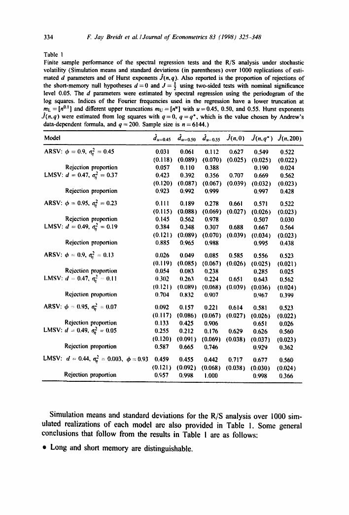
Simulation means and standard deviations over 1000 simulated realizations of each model are given for the spectral regression test in Table I. The table also presents the proportion of rejections of the short-memory null hypothesis d = 0, using the standard t-test with nominal significance level 0.05. Some conclusions t'rom the results reported in Table I are as tbllows:

® Under the short-memory null, the size of the test is not far from nominal if the upper truncation is taken to be less than [n°'5]; [n °45] seems to be an appropriate choice. For this sample size, larger upper truncations have little value: they distort the size under short memory and bias the point estimates under all models considered.

® The spectral regression test has high power against all the long memory models considered. Power is lower for the third and fourth LMSV models, since these models have a weaker long memory signal (i.e., a smaller value of Var(a~Z)/E"[at2]) than the first and second LMSV models.

• The point estimates of d under long memol), have large negative biases, which increase with mu, reflecting contamination by short-memory effects. Even with this downward bias, estimates of d under long memory are clearly different from those under short memory.

334 F. Jay Breidt et aL /Journal of Econometrics 83 (1998) 325-348

Table 1 Finite sample performance of the spectral regression tests and the R/S analysis under stochastic volatility (Simulation means and standard deviations (in parentheses) over 1000 replications of estimated d parameters and of Hurst exponents J(n,q). Also reported is the proportion of rejections of the short-memory null hypotheses d = 0 and J = ½ using two-sided tests with nominal significance level 0.05. The d parameters were estimated by spectral regression using the periodogram of the log squares. Indices of the Fourier frequencies used in the regression have a lower truncation at mL = [n °'! ] and different upper truncations mu = [n u] with u = 0.45, 0.50, and 0.55. Hurst exponents

J(n,q) were estimated from log squares with q = 0, q = q*, which is the value chosen by Andrew's data-dependent formula, and q = 200. Sample size is n = 6144.)

Model d,,=0.45 d,,--0.50 d,:0.55 J(n,O) J(n,q*) J(n,200)

ARSV: 0 = 0.9, ~ : 0.45

Rejection proportion LMSV: d = 0.47, a,~ = 0.37

Rejection proportion

ARSV: q~ = 0.95, ~,~ = 0.23

Rejection proportion LMSV: d = 0.49, ~ = 0.19


ARSV: cb 0.9, ~ .... 0.13

Rejection proportion LMSV: d ........ {),47, g~ ....... 0,11


ARSV: (/, :., 0,95, g~ 0,07

Rejection proportion LMSV: d ~ 0.49, #,)2 = 0.05


LMSV: d = 0.44, g~ = 0.003, ~6 : 0.93


0.031 0.061 0.112 0.627 0.549 (0.118) (0.089) (0,070) (0.025) (0.025) 0.057 0.1 !0 0.388 0.190 0.423 0.392 0.356 0.707 0.669

(0.120) (0.087) (0.067) (0.039) (0.032) 0.923 0.992 0.999 0.997

0.522 (O.O22) O.024 0.562 (0.023) 0.428

0.111 0.189 0.278 0 . 6 6 1 0 . 5 7 1 0.522 (0.115) (0.088) (0.069) (0.027) (0.026) (0.023) O. 145 0.562 0.978 0.507 0.030 0.384 0.348 0.307 0.688 0.667 0.564

(0.121) (0.089) (0.070) (0.039) (0.034) (0.023) 0.885 0,965 0.988 0.995 0.438

0,026 0.049 0.085 0.585 0.556 0.523 (0.119) (0.085) (0.067) (0,026) (0.025) (0,021) 0,054 0,083 0.238 {),285 0,025 0.302 0.263 0.224 0.651 0.643 0.562

(0.121) (0.089) (0.068) (0.039) (0.036) (0.024) 0.704 0.832 0.907 0.967 0.399

0.092 0.157 0 . 2 2 1 0,614 0.581 0.523 (0.117) (0.086) (0.067) (0.027) (0,026) (0.022) O. 133 0.425 0.906 0.651 0.026 0.255 0.212 0.176 0.629 0.626 0.560

(0.120) (0.091) (0.069) (0.038) (0.037) (0.023) 0.587 0.665 0.746 0.929 0.362

0.459 {).455 0.442 0.717 0.677 0.560 (0.121) (0.092) (0.068) (0.038) (0.030) (0.024) 0.¢~57 0.998 1.000 0.998 0.366

Simulation means and standard deviations for the R/S analysis over 1000 simulated realizations of each model are also provided in Table 1. Some general conclusions that follow from the results in Table i are as follows:

• Long and short memory are distinguishable.


• The classical Hurst exponent is substantially larger than ½ under the short memory models we have considered.

• Andrews' data-dependent formula for choice of q goes a long way toward reducing the bias of the classical Hurst exponent, though J(n, q*) is still above

i on average. ® The Hurst exponents estimated with values of q = 200 provide some robustness

against even highly correlated short memory.

The overall conclusions from these tables are that the spectral regression tests and the R/S analyses can be useful indicators of long memory in stochastic volatility, but as with any asymptotic tests, they should be interpreted with cau- tion. We recommend that additional diagnostics, in particular the shape of the estimated autocorrelation function, be used to help assess the usefulness of LMSV in any particular application.

3.3. Empirical evidence

The tests for long memory were performed over several market indexes' daily returns. The data and the designations used in the tables are as follows.

From the Center for Research in Security Prices (CRSP) tapes we used series starting on the first trading day of July 1962 and ending on the last trading day of July 1989. We computed returns for both the equally weighted and the value-weighted data, here denoted ECRSP and VCRSP, respectively.

Using the same raw data, we also constructed the excess returns series based on the monthly Treasury bill returns We tbllowed the usual simplification of assuming the riskless returns were constant within each month and subtracted these latter returns l'rom the ones in the stock market indexes.

We have also used the long series constructed by Schwert (1990), comple- mented with the more recent CRSP value-weighted index. This series, here denoted SCHWERT, spans from the first trading day of February 1885 to the last trading day of 1990.

In each case, in order to whiten the series of returns, we followed the usual practice of first removing any apparent correlation in the data, namely the day- of-the-week and the month-of-the-year effects, by applying standard filters.

For each of the series we applied the long-memory tests over the squared returns and the logarithms of the squared returns.

in the first three columns of Table 2 we show the results of the spectral regression tests. We immediately note that in almost all cases and all series the tests are highly significant, even when the high-frequency cut-off is severe (u = 0.40). Interestingly, the memory of the volatilities is reduced when the excess returns are computed. In the case of the equally weighted index the tests are less significant. In some cases, they do not reject the null of sole existence of short memory in the volatilities. We note, however, that the equally weighted indexes are economically much less sensible as representatives of the overall financial

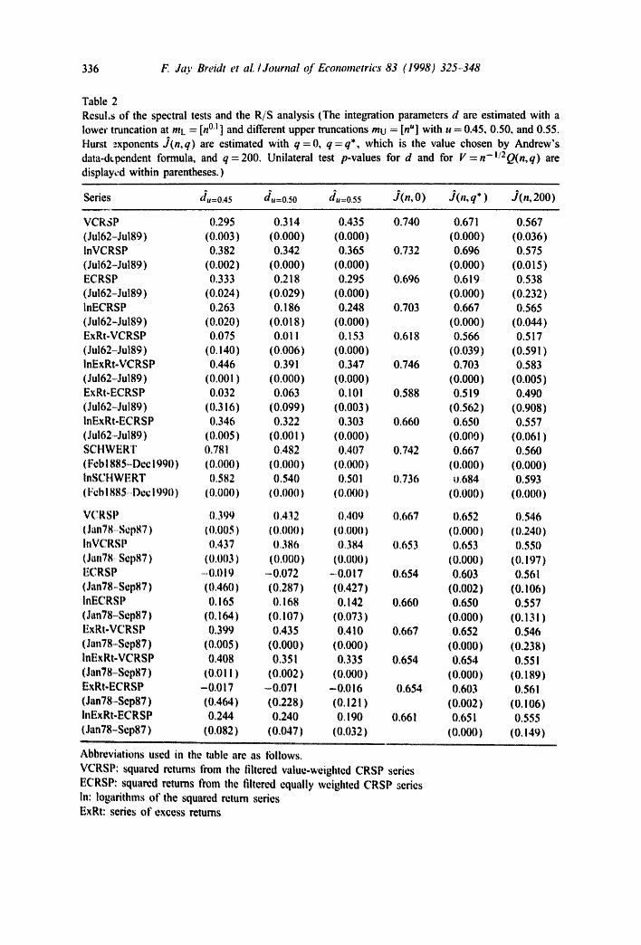
336 F Jay Breidt et al./Journal of Econometrics 83 (1998) 325-348

Table 2 Resu!,s of the spectral tests and the R/S analysis (The integration parameters d are estimated with a lower truncation at mL = [n °i ] and different upper truncations mu = [n u] with u = 0.45, 0.50, and 0.55. Hurst exponents d(n,q) are estimated with q = 0, q = q*, which is the value chosen by Andrew's data-d~pendent formula, and q=200. Unilateral test p-values for d and for V=n-l/2Q(n,q) are displayed within parentheses.)

Series du:o.45 du=o.5o d,=o.55 J(n, O) J(n,q* ) J(n, 200)

VCR3P 0.295 0.314 0.435 0.740 0.67 ! 0.567 (Jul62-Jul89) (0.003) (0.000) (0.000) (0.000) (0.036) lnVCRSP 0.382 0.342 0.365 0.732 0.696 0.575 (Jul62-Jul89) (0.002) (0.000) (0.000) (0.000) (0.015) ECRSP 0.333 0.218 0.295 0.696 0.619 0.538 (Ju162-Ju189) (0.024) (0,029) (0.000) (0.000) (0.232) inECRSP 0.263 O. ! 86 0.248 0,703 0,667 0.565 (Jul62-Jul89) (0.020) (0.018) (0.000) (0.000) (0.044) ExRt-VCRSP 0.075 0.01 ! 0.153 0,618 0.566 0.517 (Ju162-Ju189) (0.140) (0.006) (0.000) (0.039) (0.591) InExRt-VCRSP 0.446 0.391 0.347 0.746 0.703 0.583 (Ju162-Ju189) (0.001) (0.000) (0.000) (0.000) (0.005) Ex Rt-ECRSP 0.032 0.063 0. 101 0.588 0.5 ! 9 0.490 (Jul62-Jul89) (0.316) (0.099) (0.003) (0.562) (0.908) InExRt-ECRSP 0.346 0.322 0.303 0.660 0.650 0.557 (Ju162~Ju189) (0.005) (0.001 ) (0.000) (0.000) (0.061) SCHWERT 0.781 0.482 0,407 0.742 0.667 0.560 (Feb1885~Dec1990) (0 .000) ( 0 . 0 0 0 ) (0.000) (0.000) (0.000) InSCHWERT 0,582 0,540 0.501 0.736 o.684 0.593 ( Feb 1885Dcc 1990 ) ( 0,000 ) (0,000) ( 0,000 ) ( 0.000 ) (0,000)

VCRSP 0,399 (},432 0,409 0.667 (},652 0,546 ( Jan 78Sep87 ) (0,005) (0.000) (0,000) (0.000) ( 0.240 ) InVCRSP 0.437 0,386 0,384 0.653 0.653 0.550 (Jan78~Sep87) (0,003) (0.000) (0,000) (0.000) (0.197) ECRSP -0.019 -0,072 ~0.017 0,654 0.603 0.561 (Jan78~Sep87) (0.460) (0.287) (0.427) (0.002) (0.106) InECRSP 0.165 0,168 0.142 0,660 0.650 0,557 (Jan78-Sep87) (0,164) (0,107) (0.073) (0.000) (0.131) ExRt-VCRSP 0,399 0,435 0.410 0,667 0.652 0.546 (Jan78-Sep87) (0.005) (0,000) (0.000) (0,000) (0,238) InExRt-VCRSP 0.408 0,351 0,335 0,654 0,654 0.551 (Jan78-Sep87) (0.011 ) (0,002) (0,000) (0.000) (0,189) ExRt-ECRSP -0.017 -0,071 -0.016 0,654 0.603 0,561 (Jan78-Sep87) (0,464) (0.228) (0.121) (0.002) (0.106) InExRt-ECRSP 0,244 0,240 0,190 0,661 0,651 0,555 (Jan78-Sep87) (0,082) (0,047) (0,032) (0,000) (0,149)

Abbreviations used in the table are as tbllows. VCRSP: squared returns from the filtered value-weighted CRSP series ECRSP: squared returns from the filtered equally weighted CRSP series In: logarithms of the squared return series ExRt: series of excess returns

F. Jay Breidt et al./Journal of Econometrics 83 (1998)325.-348 337

markets' activity than the value-weighted ones. Finally, it is interesting to note that the log squared series reveal the existence of a considerably more significant long-memory component.

In the last three columns of Table 2 we show the estimates J(n,q) and the p-values for the statistic Y = n-I/2Q(n,q) for all the series described. All estimates point in the direction of persistent long memory. The J estimates computed with Andrews' (1991 ) data-dependent formula are highly significant for all series but the squared excess returns of the equally-weighted index. When the number of lags q increases, the significance of all statistics is reduced, as it is natural to expect in persistent processes. Even so, most of the computations show J estimates significantly larger than i.

These tests can be questioned on the grounds that long data sets may display nonstationarity in the variances and that we may be detecting nonstationarity instead of long memory. In particular, the evidence indicates this for the Schwert long indexes, since some d estimates are larger than ~. Diebold (1986), among others, interprets the findings of persistence in volatility as the outcome of shifts in the unconditional variances.

We complement the results with tests tbr shorter series, beginning with January 1978 and ending in September 1987. These shorter series avoid the crashes of 1976 and 1987 and display a period known for its relatively stable volatility.

The same tests, reproduced in the second part of Table 2, continue to reveal long memory in the conditional variances, with the exception of the already noted equally weighted index. This fact is significant and suggests that long-menaory models provide an alternative to nonstationarity tbr volatility modeling.

4. Estimating an LMSV model

The exact likelihood of the parameter vector fl given (yt . . . . . .V,,) involves an n-dimensional integral and as a consequence is extremely difficult to evalu- ate. Jacquier et al. (1994) have developed a Markov chain simulation methodol- ogy fbr likelihood-based inference in an autoregressive stochastic volatility model (ARSV). Their algorithm, a cyclic independence Metropolis chain, requires specification of prior distributions on all parameters and relies heavily on the special Markovian structure of pure autoregressive processes. Other simulation-based estimation methods for the first-order ARSV exist, see, e.g., Danielsson (1994), but it is not clear whether they apply to more general stochastic volatility models. However, these methods are computationally intensive. Here we consider simpler estimation strategies since the LMSV model is far more complicated than the ARSV model.

Other methods |br estimation from SV models have been proposed. A method of moments (MM) estimator, which avoids the problem of evaluating the likelihood function, was suggested by Taylor (1986) and Melino and Turnbull (1990).

338 F. Jay Breidt et al. /Journal of Econometrics 83 (1998) 325-348

While easy to implement, MM estimators for parameters in the ARSV model have a number of disadvantages. The MM method seems relatively inefficient when some kind of persistence in the autocorrelations is present, as it is the case of nearly nonstationary AR models (see Jacquier et al., 1994; Anderson and Soren- son, 1994, for a discussion). Moreover, the choice of appropriate moments can be problematic.

Though the process {xt } is non-Gaussian, a reasonable estimation procedure is to maximize the quasi-likelihood, or likelihood computed as if {xt } was Gaussian with ACVF 7x(h). See Nelson (1988) and Harvey et al. (1994) for discussion of QML in the context of short-memory stochastic volatility models. In the context of ARFIMA models, exact computation of the quasi-likelihood is possible (e.g., Soweli, 1992). However, it presents convergence problems and is extremely slow especially for long time series. An alternative version of this method can be conceived for LMSV models. However, the computational problems are likely to be amplified.

We suggest a spectral-domain estimator. This is a computationally simple method for which we provide an asymptotic characterization.

4. I. The spectral-likelihood est#nator

A simple alternative to maximizing the time-domain Gaussian-likelihood is to maximize its frequency-domain representation, as discussed in a long-memory context by Fox and Taqqu (1986), Dahlhaus (1989) and Giraitis and Surgailis (1990). The simulation results of Cheung and Diebold (1994) suggest that spectral-likelihood estimators have efficiency comparable to exact QML estimators when the process has an unknown mean. The following result gives the strong consistency of estimators obtained by minimizing the negative of the logarithm of the spectral likelihood ftmction,

= = log ./i~(tuk ) 4 , (11) k=,

where [.] denotes the integer part, cok = 2nkn -~ is the kth Fourier frequency, and

) ( ! ! ~ xt sin cokt

is the kth normalized periodogram ordinate. For a general justification of the method see, e.g., Beran (1994, chapter 6).

Theorem I. Assume that the parameter vector

= (d , . . . . . O , . . . . , Oq )'

is an element o f the compact parameter space t9 and assume that ~ , ( to) - ./~:(~o) ]br all ¢o in [0,n] implies that IIi =//2, where ~ ( . ) is defined 01 (10).

F. Jay Breidt et al. I Journal of Econometrics 83 (1998) 325--348 339

Let ~, minimi'_e (11) ot, er 0 and let flo denote the vector o f true parameter rabies. Then ~,, ~ flo almost surely.

The proof is provided in Appendix A.

Remarks. 1. The proof follows Dahlhaus (1989) in avoiding the special param- eterization of Fox and Taqqu (1986). Dahlhaus' (1989) result is not directly applicable to our case because his explicit assumptions include Gaussianity and his objective function is an integral version of (11). For the non-Gaussian case, we verify Dahlhaus' remark (p. 1753) that his results extend to the function (11).

2. The component 11 - e - i / [ - 2 d - - ( x / 2 - 2 cos 2)-2a of ./~(2) introduces in the likelihood a term proportional to

In/2] d ~ log(2 - 2cos~ok)2nn-l; (12)

k=!

the corresponding integral is improper, but converges to zero (see Appendix A). In the course of the proof, we show that the effect on the estimators of dropping the term (12) is negligible.

3. The identifiability condition in Theorem 1 is met if a, 2 is known from an assumed distribution for ~t; for example, ct "~ N(0, 1) implies tr, 2 = r1:2/2. If a, 2 is not known, the model is identifiable only if the ARFIMA component is not white noise; that is, if t/~ t, # 0 for some p, Oq ~ 0 for some q, or d-7¢: 0.

4.2. Finite sample properties of the spectral likelihood estimator

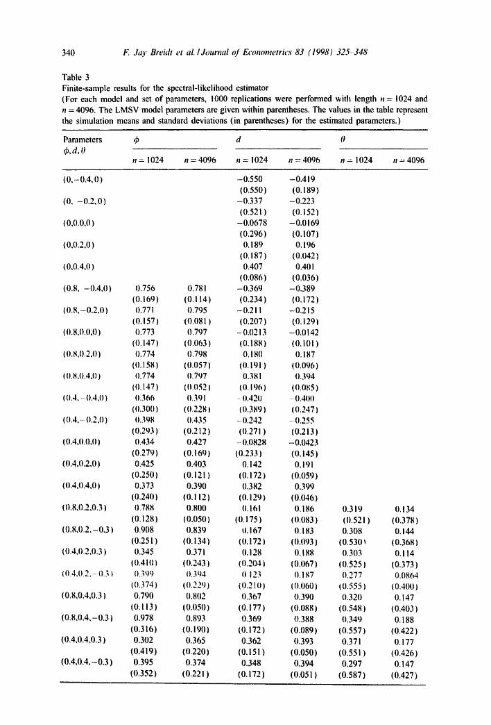
This subsection presents a simulation study of the finite sample properties of the maximum-likelihood spectral estimator previously proposed. In this experiment we consider two different sample sizes (n = 1024 and n = 4096) and three classes of LMSV models given, respectively, by ARFIMA(0, d, 0), ARFIMA(I, d, 0), and ARFIMA(I, d, 1). Within each class of models, several combinations tbr the parameters of these models are considered - see Table 3. The variance of the i.i.d, innovations in the ARFIMA component are set to one as well as the variance of the noise component.

All the results reported in this section are obtained from 1000 realizations of each model. Table 3 presents simulation means and standard deviations for the parameter estimates. Fig. I presents box plots tbr some of the models considered in the simulation. The cases considered in this figure are representative of the overall results.

Some general conclusions from the table and the box plots are:

® Maximum likelihood estimation in the spectral domain perform well for relatively large samples, such as those found in the high frequency financial markets' data.

340 F. J~o' BreMt et aL I Journal oJ Econometrics 83 (i 998) 325-348

Table 3 Finite-sample results for the spectral-likelihood estimator (For each model and set of parameters, 1000 replications were performed with length n = 1024 and n = 4096. The LMSV model parameters are given within parentheses. The values in the table represent the simulation means and standard deviations (in parentheses) for the estimated parameters.)

Parameters 4, d 0 ,b,d.O

n = 1024 n = 4096 n = 1024 n = 4096 n = 1024 n =4096

(0 , -0 .4 ,0 ) -0.550 -0.419 (0.550) 10.189)

(0, -0 .2 ,0 ) -0.337 -0.223 (0.521) (0,152)

(0,0.0,0) -0.0678 -0,0169 (0,296) 10,1071

(0,0.2,0) O. 189 O, 196 (0.187 ) (0,042)

(0,0.4,0) 0.407 0,401 (0.086) (0,036)

(0.8, -0.4,0) 0.756 0.781 -0.369 -0.389 10.1691 (0. I 14) (0.234) 10,1721

(0.8,- 0.2,0 ) 0.771 0.795 -0.211 -0,215 (0.1571 (0.081) (0.207) 10,1291

(0.8,0.0.01 0.773 0,797 -0.0213 -0,0142 (0,147) (0.063) (0.188) (0.1011

(0,8,0.2.0) 0.774 0.798 O. 180 0,187 (0,158) (0,057) 10.1911 (0.096)

(1), 8,0,4,0 ) O, 774 0,797 0,381 0,394 (0,147) (11,052) ((1,196) (0,(1~;51

(0,4,. 0,4,0 ) O, 36i', 0,391 ....... 0,4211 --1),41)11 (0,300) (0,228) (0,389) (0,247)

(0,4, 0,2,0) 0,398 0,435 -0.242 ...... 0!55 (0.293) (11.2121 10.271 ) 10,213)

(0,4,0,0,0) 11,434 0.427 -.0.0828 -0.0423 (0,279) (0.169) (0.233) (0.1451

( 0,4,0,2,0 ) 0.425 0.403 O. 142 O, 191 (0.250) (0.1211 (0.1721 (0,059)

10.4,0.4,01 0.373 0.390 0.382 0,399 (0.240) (0. I 12) 10.1291 (0.046)

(0,8,0,2,0,3) (I.788 0,800 0.161 0,186 (0,128) (0,050) (0,175) (0,083)

(0.8.0.2. -0.3 ) 0,908 0.839 O. 167 0.183 10.251) (0.134) (11.172) (0.093)

(0.4,0.2,0.3) 0.345 0.371 0.128 0,188 (0.410) (0.243) (0.204) (0.067)

(0.4.0,2.--0.3 ) 0,30 t) O. 3t14 O. 123 O. 187 (11,374) (0.2291 (0.210) (0.060)

(0,8,0.4,0.3) 0.790 0.802 0.367 0,390

(0.113) (0.050) (0.177) (0.088) (0.8,0.4,-0.3) 0.978 0.893 0.369 0.388

(0,316) (0.190) 10.172) (0,089) (0,4,0.4,0,3) 0.302 0.365 0.362 0,393

(0,419) (0.220) (0.151) (0,050) (0.4,0,4,-0,3) 0.395 0,374 0.348 0,394

(0.352) (0,221 ) (0.172 ) (0,051 )

0.319 0,134 (0,521) (0.378) 0.308 0.144

(0.530~ (0.368) 0.303 0,114

( 0.525 ) ( 0.373 ) 0.277 0.0864

( 0.555 ) ( 0.400 ) 0.320 0.147 (0.548) (0.403) 0.349 0.188 (0.557) (0.422) 0.371 0.177

(0.551) (0.426) 0.297 O. 147 (0.587) (0.427)

F. Jay Breidt et at,. IJounzal of Econometrics 83 (1998) 325-348 341

"10 I

( ' O

1

0

-1

-2

-3

-4

-5

d=-0 .4 d=O.O d=0.4

1.0 o °

0.2 • - 0 . 2

"O -0.6 I I - 1 . 0

('to II : - ! . 4

; - I . e -2.2 -2.6 1024 4096

Length of series

0.4 m

0.3

02

0 0.1 I

m • ((D -0.o Iz

• -0 .1 !

I -o.2 =

-0.,,3 1024 4096 Length of series

+ t024 4096

Length of series

"10 I

('D

0.4

0.2

=0.0

-0.2

- 0 .4

-0.6

- 0 , 6

E3+ m

l i |

1024 4096 Length of series

d=0.4, ¢=0.4

0.6

0.4

0.2

0 -0.0 I

( 0 -0.2

- 0 . 4

-0.6

-0.8 1024 4096 Length of series

"O I

( 'O

ct=0.2, 0=0.4, 0 - - 0 . 3

IO 08 0,6 04 02

-0.0 -0,2 - 0 4 -06 -0.6 -1,0

. 0.8 i

. 04

i i `~ .0 -0.0 I - 0 ,4 (O

-0.8

=i.2

-I.6 lo24 4096 Length of series

|

I

3,0 2,5 2.0

0 1,5 I 1.0

((D 05 0.0

-0.5 - I 0 -1.5

=

|

1024 4096 1024 4096 Length of series Length of series

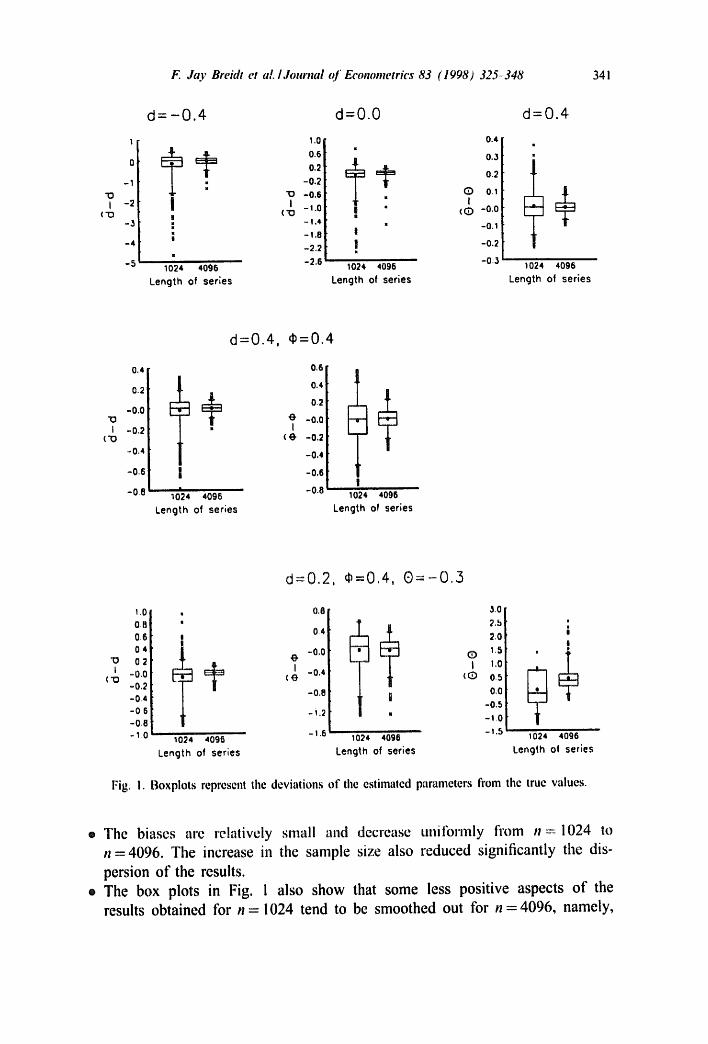
Fig, !. Boxplots represent the deviations of tile estirnated parameters fforn tile true values.

o The biases arc relatively small and decrease uniformly from n = 1024 to n = 4096. The increase in the sample size also reduced significantly the dis- persion of the results.

® The box plots in Fig. I also show that some less positive aspects of the results obtained for n = 1024 tend to be smoothed out for n = 4096, namely,

342 F Jay Breidt et aL /Journal o f Econometrics 83 (1998) 325-348

the asymmetry of the distribution of the estimates. An extreme case was the LMSV model with an ARFIMA(0, -0.4, 0) component.

® The maximum-likelihood spectral estimator provides less biased and more pre- cise parameter estimates in processes in which the fractional parameter d was positive. This includes both the estimate of d and the estimates of the other parameters in the model.

• The performance of the maximum-likelihood spectral estimator in small samples might be less than ideal as is illustrated by the box plots of the smaller sample size. Moreover, some very large outlie~s occurred when n = 1024.

® The procedure encountered some difficulties in estimating the moving average term, even when the number of observations was 4096 (although the magnitude of the problem decreased for the larger sample size).

Given the overall good performance of the estimator when n = 4096, these sam- pling experiments indicate that maximum-likelihood spectral estimation of LMSV models may be a very effective method for the type of financial applications that have led to this line of research.

Moreover, this maximum-likelihood estimator is easy to implement. Conver- gence for a LMSV model with an ARFIMA(0, d, 0) component and n=4096 was typically attained in less than 20 iterations and less than 4 s of CPU time on a Pentium 100 MHz. 6

43. Modelinff rolatility t~'stock returns

Nelson (1991) introduces the EGARCH model using as an example the daily returns Ibr the value-weighted market index from the CRSP tapes for July 1962- December 1987. He selects an ARMA(2, I) model lbr log ~2 and linds the largest estimated AR root to be 0.99962, suggesting substantial persistence.

For comparison, we littcd a model with long-memory stochastic volatility to the log squares of the VCRSP series described in Section 3.3 above This log squared series, denoted {xt }, consists of n = 6801 mean-corrected observations modeled as

Xt ~ t~t "4" i:t,

where {,:t} is i.i.d. (O,q: 2) independent of {c,} and {r,} is the ARFIMA(I, d, 0),

( I - B)'t( I - ,bB)ct = ~lt,

with {'l, } i.i.d. (0, a,~ ).

t, in these simulations w¢ used the set of routines for maximum likelihood estimation provided by the GAUSS programming language. The algorithm used is the derivative-based procedure of Broyden, Fletcher, Goldfarb, and Shanno, as described in the GAUSS manual. Analytical derivatives were provided, The code is available from tile authors upon request.

F. Jay Breidt et aL /Journal of Economeo'ic~" 83 (1998) 325-348 343

ci

ci

ci

c i

<o ci"

d

0 d"

°-0 " 5'0 lCIO 1',S0 2C)0"

Fig. 2. Empirical and fitted autocorrelation functions for the log squares VCRSP series.

The spectral likelihood tbr the xt's was formed as in Eq. ( ! ! ) replacing (12) with zero, which we have ibund useful though this needs further investigation. 'l'he resulting likelihood was maximized with respect to the parameters a,~, d, ~/~

-2 and q~ yielding the estimates a,, = 0.00318, d = 0.444, ~ = 0.932 and 42 = 5.238. Fig. 2 shows the empirical and fitted autocon'elations for the series {xt}.

The empirical autocorrelations show a slow decay, remaining non-negligible for hundreds of lags. The ACF of the fitted LMSV model was derived from the ARFIMA( I, d, O) fonnulae in Hosking (1981) and adjusted for the bias due to the existence of long memory as in Theorem 5 of Hoskinlt; (1995). In Fig. 2, the bias-adjusted ACF for LMSV accurately reflects the slow decay of the empirical ACF.

We also fitted short-memory GARCH and EGARCH models as well as an IGARCH model to the same VCRSP series, in order to compare the properties of fitted GARCH, IGARCH, EGARCH, and LMSV models with the observations, we computed the autocorreiations of the fitted models and plotted them against the sample atttocorrelations of the series. The order of the models was selected by SIC.

As it is often observed in practice, the fitted GARCH and IGARCH are very similar: SIC selected a GARCH(I,2) and an IGARCH(I,2). The fitted

344 F. Jto' Breidt et al. /Journal of Etonometrics 83 (1998) 325-348

GARCH had parameter estimates 6l =0.923,/~i =0.143, and b2 =-0 .067 . Their sum is 0.999. The fitted IGARCH has parameter estimates ti=0.923,/~l =0.145, and /~_~ = - 0.068. Using the GARCH parameter estimates, we simulated 1,000 GARCH realizations, each of length n = 6801, and computed the sample ACF of the log squares for each realization. The same simulations were done for IGARCH. The average of the GARCH sample ACF's, plotted in Fig. 2 and la- beled 'GARCH/IGARCH', is almost indistinguishable from the average of the IGARCH sample ACF's (not plotted). The GARCH models, nearly integrated or integrated, seem 'too persistent' to model these data.

The SIC criterion selected an EGARCH(2, 0). The fitted EGARCH had parameter estimates t~! =0.0185, t~2 =0.200, ~b I =0.577 and t~., =0.359. The ACF for the log squares corresponding to the fitted EGARCH model was obtained theoret- ically through the formulae derived in Appendix B. The short-memory EGARCH model clearly fails to reflect the slow decay of the empirical ACF.

5. Conclusions

Empirical evidence suggests that the recent interest in long-memory conditional variance models tbr stock market indices is well-founded. We find evidence of long memory in variance proxies using both a nonparametric and semiparametric test tbr many series. A simulation exercise shows that these tests are able to distinguish long from short memory in the volatilities.

The long memory stochastic volatility (LMSV)model is an analytically tractable model of this persistence in the conditional variances. The LMSV is easily fitted and analyzed using standard tools tbr weakly stationary processes, in particular, the LMSV model is built from the widely used ARFIMA class of long- memory time series models, so that many of its properties arc well-understood. The spectral-likelihood estimator proposed tbr this model is strongly consistent and finite-sample simulation results show it has reasonable properties tbr series of the length usually tbund in financial data.

An example with a long series of stock prices shows that short-memory models are unable to reproduce more than the short-term structure of the autocorrelations, in contrast, a parsimonit, us LMSV model fit to the data is able to reproduce closely the empirical autocorrelation structure of the conditional volatilities.

These results are encouraging and suggest some avenues lbr future research. We believe it would be interesting to investigate further the empirical relevance of the LMSV model, namely, its relevance tbr estimating and tbrecasting the volatilities and pricing derivatives. We also believe that it would be useful to compare properties of the LMSV with other models of persistence in the volatilities.

F. Jay BreMt t,t aL /Journal +!/' Econometrics 83 (1998) 325- 348 345

Appendix A. Proof of strong consistency for spectral-likelihood estimators

Let/~,, minimize (11) and let

~( f l ) = 2 logj~(o~) + h,,(~o) ~(to) } dog,

where fl0 denotes the vector of true parameter values. Then

+

~< [n/2l fOrc 2rtn-I ~ gidtok ) - 2 k=l

+

In/21 ~°rc I 2rcn- I ~ d log(2 - 2 cos to, ) - 2 d log(2 - 2 cos to) dro ~=1 2~,1 -I 1~1 ln(tOk) 2 f0 n ]i~"(t'))dto

hook) .

= Ml, , ( f l )+ M2,,(fl)+ M3,,(fl),

where

gl~(} . )=log{~'O(e- i ; )12+tr ,~ '~(e- i ; )12 ' l - e-i;" 2d } 2rtl,/,(e-i; ) -'

Now Ml,,(fl) converges to zero uniformly in fl by Riemann inlegrability of C.l#(+,J), continuity in fl of the integral and cmnpactness of (9. Given 6 > 0 , Ml,,(fl) can be bounded above and below by the upper Riemann sum plus 6 and tile lower Rie,nann sum minus 6 for a partition .g, of [0,re], where .',4, comains the mh- order Fourier ti~equencies and .'P,, c .~,~i c . . . . For each fl, these bounds converge to zero :t:: r~i monotonically, and so uniform convergence in fl t'ollows by Dini's theorem.

Next, Ma,,(fl) can be bounded uniformly in fl by

I.,'21 fO n [ 0.5 2nn- I ~ log(2 - 2 cos v~ ) - 2 log(2 - 2 cos.J) doJ ,

k=l

which converges to zero since

.L ~ log(2 - 2 cos t,~) dt,J = O.

Finally, M3,,(fl) can be shown to converge almost surely (a.s.) to zero uni- tbrmly in fl by modifying Lemma I of Hannan (1973) (see also Lemrna I of Fox and Taqqu, 1986; Dahlhaus, 1989). First, l/./it(to) satisfies the continuity

346 F. Jay Breidt et aL /Journal of Econometrics 83 (1998) 325-348

condition of HannaH (1973) and so the C6saro sum of its Fourier series converges uniformly in (t~,fl) for fl E O. Second, the process {xt} is ergodic since {vt } is a linear process with i.i.d, innovations and square-summable coefficients (e.g., HannaH, 1970, p. 204) and {~:t} is i.i.d., independent of {vt}. From these two facts, Lemma 1 of HannaH (1973) follows.

Hence,

sup I~, , (P) - ~(P) t ---' o a.s. / ~ 0

Since - logx t> 1 - x, with equality holding if and only if x = !,

,~(fl) = 2 fo '~

~>2fo ~

= 2 ~ ~

- log A'(°~) ~. (~o) } ~(~o----S + log A,(,:o) + h(o~ )

.];~((o) + I°gh"(~o) ~ ~j(o9)

{ logJi~,,(¢o) -t ];~,,(co) } d¢o

= ~(Po) ,

dco

and so (using the identifiability condition)/'k) uniquely minimizes .~(/~). Thus

• ~ , ( / } , , ) ~ < , ~ ; , ( P o ) and ,'./'(fl0)~< ~'(1},,),

¢" " ' S which implies that Y(#,,)--, 'd"lfl0) a ..... and theretbre also ft, ~ rio a.s. by com- pactness of O. [1

Appendix B. Autocovariance function of log ,squares under EGARCH

Under an EGARCH model for {Y,}, the ACVF for the series {xt} = {Iogy 2 - Pt}, where {/it} are the deterministic volatility changes in Eq. (3), can be computed as follows:

Cov(xt , Xt ~th )

= C o y ~ a ( ~ , - ; - , ) + log ..2 .2 • ~.,, ~ ~.q(¢,+h--i-~ ) + log ;,.,.h i = o i = o

= Var{,q(~,)};,th)+ ff~,_ ~ E[,q(#,)log #~l + Var(log #~)i{h~,~o},

where ;,(h) is the autocovariance fimction

/ = 0

F. Jto' Breidt et al./Journal of Econometrit's 83 (1998) 325-348 347

and ~b-i := O. If, as it was originally suggested by Nelson (1991), the function g(-) is chosen to be

o(~,) = 6~¢, + 62(1~,1- EIC, I),

then we have

Var{g(~,)} =6~ + 62(1 -- E21C, I).

For Gaussian et, EI ,I= Var(iog~t2)=n2/2 and

E [ g ( ~ , ) l o g ~ ] = 262 ( log2 - x + 1.27), "

where x _~ 0.577216 is Euler's constant. Thus, if 62 - O , the Gaussian EGARCH ACVF has the same form as the SV ACVF in (7).

References

Andrews, D.W.Q., 1991. Heteroskedasticity and atttocorrelation consistent covariance matrix estimation. Econometrica 59, 817-858.

Anderson, T.G., Sarenson, B.E., 1994. GMM and QML asymptotic standard deviations in stochastic volatility models: a response to Ruiz. Working Paper 189, Department of Finance, Kellog School, Northwestern University.

Baillie, R.T., 1996. Long-memory processes and fractional integration in econometrics. Journal of Econometrics 73, 5~o59.

Baillie, R.T., Bollerslev, T., Mikkelsen, H O., 1996. Fractionally integrated generalized autoregressive conditional heteroskedasticity. Journal o1" Econometrics 74, 3 3 0 .

I:]erlllrl. J., It)94. Statistics Ibr Long-Memory Processes. Chapman & Hall, New York. 13ollerslev, T., 1986. Generalized autoregressive conditional heteroskedaslicity. Journal of Fcono-

metrics 31, 307=327. Bollerslev, T., Chou, R.Y., Kroner, K.F., 1992. ARCH modeling in linance. Journal of Econometrics

52, 5-59. Bollerslev, T., Mikkelsen, tI,O.A., 1990. Modeling ~md pricing long-memory in stock market volatility.

Journal of Econometrics 73, 15 !-I 84. Breidt, F.J., Crato, N,, de Lima, P., 1994. Modeling long memory stochastic volatility. Working

Papers in Economics No. 323, Johns Hopkins University. Brockwell, P.J., Davis, R.A., 1991. Time Series: Theory and Methods, 2nd ed. Springer, New York. Cheung, Y.W., 1993. Tests tbr fractional integration: a Monte Carlo investigation. Journal of Time

Series Analysis 14, 331-345. Cheung, Y.W., Diebold, F.X., 1994. On maximum likelihood estimation of the differencing parameter

of fractionally-integrated noise with unknown mean. Journal Econometrics 62, 301-3 16. Dahlhaus, R., |989. Efficient parameter estimation for sell=similar processes. Annals of Statistics 17,

1749 -1766 Danielsson, J., 1994. Stochastic volatility in asset prices: estimation with simulated maximum

likelihood. Journal of Econometrics 64, 375-400. de Lima, P.J.F., Crato, N., 1993. Long-range dependence in the conditional variance of stock returns.

August 1993 Joint Statistical Meetings, San Francisco. Proceedings of the Business and Economic Statistics Section.

348 F. Jay BreMt et al./Journal of Econometrics 83 (1998) 325-348

Diebold, F.X., 1986. On modeling the persistence of conditional variances. Econometric Reviews 5, 51-56.

Ding, Z., Granger, C., Engle, R.F., 1993. A long memory property of stock market returns and a new model. Journal Empirical Finance !, 83-106.

Engle, R.F., 1982. Autoregressive conditional heteroskedasticity with estimates of the variance of United Kingdom inflation. Econometrica 50, 987-1007.

Fox, R., Taqqu, M.S., 1986. Large-sample properties of parameter estimates for strongly dependent stationary Gaussian time series. Annals of Statistics 14, 517-532.

Geweke, J., Porter-Hudak, S., 1983. The estimation and application of long memory time series models. Journal of Time Series Analysis 4, 221-238.

Giraitis, L., Surgailis, D., 1990. A central limit theorem for quadratic forms in strongly dependent linear variables and its application to asymptotical normality of Whittle's estimate. Probability Theory and Related Fields 86, 87-104.

Granger, C.W., Joyeux, R., 1980. An introduction to long-memory time series models and fractional differencing. Journal of Time Series Analysis !, 15-29.

Hannah, E.J., 1970. Multiple Time Series. Wiley, New York. Hannan, E.J., 1973. The asymptotic theory of linear time-series models. Journal of Applied Probability

!0, 130-145. Harvey, A.C., 1993. Long memory in stochastic volatility. Mimeo, London School of Economics. Harvey, A.C., Ruiz, E., Shephard, N., 1994. Multivariate stochastic variance models. Review of

Economic Studies 61,247°-264. Hosking, J.R.M., 1981. Fractional differencing. Biometrika 68, 165-176. Hosking, J.R.M., 1995. Asymptotic distributions of the sample mean, autocovariances and

autocorrelations of long-memory time series. Journal of Econometrics, tbrthcoming. Jacquier, E., Poison, N.G., Rossi, P.E., 1994. Bayesian analysis of stochastic volatility models (with

discussion). Journal of Business and Economic Statistics 12, 371-417. Lo, A.W., 1991. Long-term memory in stock market prices. Econometrica 59, 1279-1313. Mandelbrot, B.B., Taqqu, M., 1979. Robust R,/S analysis of long-run serial correlation. Proceedings

of tile 42nd Session of the International Statistical Institute, International Statistical Institute. Melino, A, Turnbull, S.M., 1990. Pricing foreign currency options with stochastic volatility. Journal

ECOl~Ot~nctrics 45, 239 265. Nelson, D.B., 1988, Time series behavior ot' stock market volatilily and returns. I)h.i). tlisserlalion,

Economics l)epanmenl, Massachus¢lts Inslitute of Technology. Nelson, D,B,, 1991. Conditional heteroskedasticity in asset returns: a new approach. Econometrica

59, 347~370. Robinson, P.M., 1991 Testing tbr strong serial com, lation and dynamic conditional heteroskedasticity

in multiple regression. Journal of Econometrics 47, 67-84. Robinson, P.M., 1995. Log-periodogram regression of time series with long range dependence. Annals

of Statistics 23, 1048-1072. Schwert, G.W., 1990. indexes of U.S. stock prices t'rom 1802 to 1987. Journal of Business 63,

399-426, Sowell, F., 1992. Maximum likelihood estimation of stationary univariate ti'actionally integrated time

series models. Journal Econometrics 53, ! 65-188. Taylor, S., 1986. Modelling Financial Time Series. Wiley, New York. Taylor, S., 1994. Modeling stochastic volatility: a review and comparative study. Mathematical

Finance 4, 183 ~204. Wisharl, J,, 1947, The cumulanls of t i le : and of the logarithmic /2 and t dis,,0utions. Biometrika

34, 170 178.

The detection and estimation of long memory in stochastic volatility

Documents

Transcript of The detection and estimation of long memory in stochastic volatility