Robotic Path Planning for High-Level Tasks in Discrete ...

Robotic Path Planning forHigh-Level Tasks in Discrete

Environments

by

Frank Imeson

A thesispresented to the University Of Waterloo

in fulfilment of thethesis requirement for the degree of

Doctor of Philosophyin

Electrical and Computer Engineering

Waterloo, Ontario, Canada, 2018

c© Frank Imeson 2018

Examining Committee Membership

The following served on the Examining Committee for this thesis. The decision of theExamining Committee is by majority vote.

External Examiner: Ibrahim Volkan IslerProfessor

Supervisor: Stephen L. SmithAssociate Professor

Internal Examiner: Dana KulicAssociate Professor

Internal Examiner: Wojciech GolabAssistant Professor

Internal Examiner: Steven WaslanderAssociate Professor

ii

I hereby declare that I am the sole author of this thesis. This is a true copy of the thesis,including any required final revisions, as accepted by my examiners.

I understand that my thesis may be made electronically available to the public.

iii

Abstract

This thesis proposes two techniques for solving high-level multi-robot motion planningproblems with discrete environments. We focus on an important class of problems thatrequire an allocation of spatially distributed tasks to robots, along with a set of efficientpaths for the robots to visit their task locations. The first technique, SAT-TSP, mod-els the problem with a framework that allows a natural coupling between the allocationproblem and the path planning problem. The allocation problem is encoded as a BooleanSatisfiability problem (SAT) and the path planning problem is encoded as a TravellingSalesman Problem (TSP). In addition, this framework can handle complex constraintssuch as battery life limitations, robot carrying capacities, and robot-task incompatibilities.We propose an algorithm that leverages recent advances in Satisfiability Modulo Theoryto combine state-of-the-art SAT and TSP solvers. We characterize the correctness of ouralgorithm and evaluate it in simulation on a series of patrolling, periodic routing, andmulti-robot sample collection problems. The results show that our algorithm outperformsa state-of-the-art mathematical programming solver on a majority of the problems in ourbenchmark, especially the more difficult problems.

The second technique, Γ-Clustering, is used to reduce the computational effort of findinggood solutions for metric discrete path planning problems. This technique can be used onthe set of allocation path planning problems that do not have ordering constraints (orderingonly affects the cost of the solution, not its feasibility). To obtain the computationalsavings, we find Γ-Clusters within the problem’s environment and then restrict how feasiblepaths visit these clusters. We prove that solutions found using this approach are withina constant factor of the optimal. By increasing the parameter Γ we can improve thequality of the bound but we do so with less computational savings. We provide a simplepolynomial-time algorithm for finding the optimal Γ-Clustering and show that for a givenΓ the clustering is unique. We provide two methods for using Γ-Clusters on path planningproblems, a coupled method and a hierarchical method. We demonstrate the effectivenessof these methods on travelling salesman instances, sample collection problems, and periodrouting problems. The results show that for many instances we obtain significant reductionsin computation time with little to no reduction in solution quality. Comparing thesemethods to a standard integer programming approach reveals that as the problems becomemore difficult, the solution quality of the two methods degrade at a slower rate than thestandard approach, thus for more difficult instances we can use Γ-Clustering to find higherquality solutions.

iv

Acknowledgements

I would like to thank my PhD supervisor Stephen L. Smith; my Masters supervisors Sid-dharth Garg and Mahesh Tripunitara; and my PhD committee Ibrahim Volkan Isler, DanaKulic, Vijay Ganesh, Wojciech Golab, and Steven Waslander.

v

Dedication

I dedicate my thesis to my mother. Thank you for your guidance, encouragement, andsupport.

vi

Table of Contents

Table of Contents x

List of Tables . . . . . . . . . . . . . . . . . . . . . . . . . . . . . . . . . . . . . xi

List of Figures . . . . . . . . . . . . . . . . . . . . . . . . . . . . . . . . . . . . . xiii

1 Introduction 1

1.1 Literature Survey . . . . . . . . . . . . . . . . . . . . . . . . . . . . . . . . 3

1.2 Contributions . . . . . . . . . . . . . . . . . . . . . . . . . . . . . . . . . . 4

2 Preliminaries 7

2.1 Graphs . . . . . . . . . . . . . . . . . . . . . . . . . . . . . . . . . . . . . . 7

2.2 The Travelling Salesman Problem . . . . . . . . . . . . . . . . . . . . . . . 8

2.3 Complexity Theory . . . . . . . . . . . . . . . . . . . . . . . . . . . . . . . 8

2.3.1 Decision Problems . . . . . . . . . . . . . . . . . . . . . . . . . . . 9

2.3.2 Complexity Classes . . . . . . . . . . . . . . . . . . . . . . . . . . . 9

2.4 Using ILP to Find Solution Paths . . . . . . . . . . . . . . . . . . . . . . . 10

2.5 Summary . . . . . . . . . . . . . . . . . . . . . . . . . . . . . . . . . . . . 11

3 An Alternative to ILP 13

3.1 Related Work . . . . . . . . . . . . . . . . . . . . . . . . . . . . . . . . . . 14

3.2 Background . . . . . . . . . . . . . . . . . . . . . . . . . . . . . . . . . . . 16

3.2.1 Boolean Satisfiability (SAT) . . . . . . . . . . . . . . . . . . . . . . 16

vii

3.2.2 Boolean Circuits . . . . . . . . . . . . . . . . . . . . . . . . . . . . 16

3.2.3 SMT and DPLL(T) . . . . . . . . . . . . . . . . . . . . . . . . . . . 17

3.2.4 Induced Subgraphs . . . . . . . . . . . . . . . . . . . . . . . . . . . 18

3.3 Problem Statement . . . . . . . . . . . . . . . . . . . . . . . . . . . . . . . 18

3.3.1 SAT-TSP Definition . . . . . . . . . . . . . . . . . . . . . . . . . . . 18

3.3.2 Complexity of SAT-TSP . . . . . . . . . . . . . . . . . . . . . . . . 20

3.4 CBTSP: An SMT-based approach for SAT-TSP . . . . . . . . . . . . . . . . 21

3.4.1 The BRUTE Approach: A Lead-in to CBTSP . . . . . . . . . . . . . 22

3.4.2 The CBTSP Solver . . . . . . . . . . . . . . . . . . . . . . . . . . . 23

3.4.3 Correctness . . . . . . . . . . . . . . . . . . . . . . . . . . . . . . . 27

3.4.4 Relaxing TSP-monotonicity . . . . . . . . . . . . . . . . . . . . . . 29

3.5 An Integer Program Formulation . . . . . . . . . . . . . . . . . . . . . . . 31

3.6 Applications . . . . . . . . . . . . . . . . . . . . . . . . . . . . . . . . . . . 33

3.6.1 Patrolling . . . . . . . . . . . . . . . . . . . . . . . . . . . . . . . . 33

3.6.2 Sample Collection . . . . . . . . . . . . . . . . . . . . . . . . . . . . 36

3.6.3 Periodic Routing . . . . . . . . . . . . . . . . . . . . . . . . . . . . 39

3.7 Experiments . . . . . . . . . . . . . . . . . . . . . . . . . . . . . . . . . . . 40

3.7.1 Simulations . . . . . . . . . . . . . . . . . . . . . . . . . . . . . . . 41

3.7.2 Patrolling . . . . . . . . . . . . . . . . . . . . . . . . . . . . . . . . 41

3.7.3 Sample Collection . . . . . . . . . . . . . . . . . . . . . . . . . . . . 44

3.7.4 Period Routing . . . . . . . . . . . . . . . . . . . . . . . . . . . . . 46

3.8 Summary . . . . . . . . . . . . . . . . . . . . . . . . . . . . . . . . . . . . 47

4 Pruning Solutions 49

4.1 Related Work . . . . . . . . . . . . . . . . . . . . . . . . . . . . . . . . . . 51

4.2 Background . . . . . . . . . . . . . . . . . . . . . . . . . . . . . . . . . . . 53

4.2.1 Clusters . . . . . . . . . . . . . . . . . . . . . . . . . . . . . . . . . 53

4.2.2 Search Space . . . . . . . . . . . . . . . . . . . . . . . . . . . . . . 54

viii

4.2.3 Multigraphs . . . . . . . . . . . . . . . . . . . . . . . . . . . . . . . 54

4.3 Path Planning Problem Statement . . . . . . . . . . . . . . . . . . . . . . 55

4.4 Γ-Clustering . . . . . . . . . . . . . . . . . . . . . . . . . . . . . . . . . . . 56

4.4.1 Definitions . . . . . . . . . . . . . . . . . . . . . . . . . . . . . . . . 56

4.4.2 Finding Γ-Clusters . . . . . . . . . . . . . . . . . . . . . . . . . . . 57

4.5 Coupled Planning . . . . . . . . . . . . . . . . . . . . . . . . . . . . . . . . 60

4.5.1 Search Space Reduction . . . . . . . . . . . . . . . . . . . . . . . . 61

4.5.2 Solution Quality Bounds . . . . . . . . . . . . . . . . . . . . . . . . 63

4.6 Decoupled Planning . . . . . . . . . . . . . . . . . . . . . . . . . . . . . . . 72

4.6.1 Search Space Reduction . . . . . . . . . . . . . . . . . . . . . . . . 74

4.6.2 Solution Quality Bounds . . . . . . . . . . . . . . . . . . . . . . . . 77

4.7 Hierarchical Planning . . . . . . . . . . . . . . . . . . . . . . . . . . . . . . 79

4.7.1 A Hierarchical Method for TSP Problems . . . . . . . . . . . . . . . 80

4.7.2 A Hierarchical Method for Non-TSP Problems . . . . . . . . . . . . 84

4.8 Experiments . . . . . . . . . . . . . . . . . . . . . . . . . . . . . . . . . . . 86

4.8.1 Problem Library . . . . . . . . . . . . . . . . . . . . . . . . . . . . 86

4.8.2 Setup and Execution . . . . . . . . . . . . . . . . . . . . . . . . . . 87

4.8.3 Path planning with Γ-Clusters . . . . . . . . . . . . . . . . . . . . . 89

4.8.4 Other Clustering Methods . . . . . . . . . . . . . . . . . . . . . . . 93

4.9 Summary . . . . . . . . . . . . . . . . . . . . . . . . . . . . . . . . . . . . 94

5 Conclusions 96

5.1 Future Work . . . . . . . . . . . . . . . . . . . . . . . . . . . . . . . . . . . 97

5.1.1 SAT-TSP . . . . . . . . . . . . . . . . . . . . . . . . . . . . . . . . . 97

5.1.2 Γ-Clustering . . . . . . . . . . . . . . . . . . . . . . . . . . . . . . . 98

References 100

Appendices 110

ix

Appendix A CBTSP Solver Parameters 111

Appendix B Additional SAT-TSP Approaches 115

B.1 The constraint satisfaction problem (CSP) . . . . . . . . . . . . . . . . . . 115

B.2 Search Algorithms . . . . . . . . . . . . . . . . . . . . . . . . . . . . . . . 116

B.3 HCP to SAT . . . . . . . . . . . . . . . . . . . . . . . . . . . . . . . . . . . 119

B.4 Solver Approaches . . . . . . . . . . . . . . . . . . . . . . . . . . . . . . . 122

B.4.1 Reduction to SAT . . . . . . . . . . . . . . . . . . . . . . . . . . . . 122

B.4.2 Reduction to TSP . . . . . . . . . . . . . . . . . . . . . . . . . . . . 123

B.4.3 Reduction to GTSP . . . . . . . . . . . . . . . . . . . . . . . . . . . 125

B.4.4 Reduction to CSP . . . . . . . . . . . . . . . . . . . . . . . . . . . . 128

B.4.5 Reduction to SMT . . . . . . . . . . . . . . . . . . . . . . . . . . . . 128

B.5 Benchmark Problems . . . . . . . . . . . . . . . . . . . . . . . . . . . . . . 128

B.5.1 SatLib . . . . . . . . . . . . . . . . . . . . . . . . . . . . . . . . . 129

B.5.2 TspLib . . . . . . . . . . . . . . . . . . . . . . . . . . . . . . . . . 129

B.5.3 HardLib . . . . . . . . . . . . . . . . . . . . . . . . . . . . . . . . 130

B.5.4 SetLib . . . . . . . . . . . . . . . . . . . . . . . . . . . . . . . . . 130

B.5.5 GTspLib . . . . . . . . . . . . . . . . . . . . . . . . . . . . . . . . 130

B.5.6 GTspLib+ . . . . . . . . . . . . . . . . . . . . . . . . . . . . . . . 130

B.5.7 CountLib . . . . . . . . . . . . . . . . . . . . . . . . . . . . . . . 131

B.5.8 OrderedLib . . . . . . . . . . . . . . . . . . . . . . . . . . . . . . 131

B.5.9 MultiRobotLib . . . . . . . . . . . . . . . . . . . . . . . . . . . . 132

B.6 Benchmark Results . . . . . . . . . . . . . . . . . . . . . . . . . . . . . . . 134

B.6.1 Unsuccessful Approaches . . . . . . . . . . . . . . . . . . . . . . . . 135

B.6.2 GTSP Approach . . . . . . . . . . . . . . . . . . . . . . . . . . . . . 136

B.6.3 CSP Approach . . . . . . . . . . . . . . . . . . . . . . . . . . . . . . 136

B.6.4 BRUTE Approach . . . . . . . . . . . . . . . . . . . . . . . . . . . . 137

x

List of Tables

3.1 Experimental results for patrolling problem instances (300 second trials).The left three columns indicate the patrolling instance number, the numberof observation locations (n), and the number of points of interest (m) in theenvironment. The best results are shown in bold. . . . . . . . . . . . . . . 42

3.2 Experimental results for sample collection instances (300 second trials). Onthe left we indicate the instance number, the number of samples (n), andthe maximum number of different minerals (m) in the environment. Thebest results are shown in bold. Results that are shown with a dash indicatethat the solver was not able to solve the instance. . . . . . . . . . . . . . . 45

3.3 Experimental results for period routing problem instances (300 second tri-als). The left two columns indicate the instance number and the number oflocations in the environment. The best results are shown in bold. . . . . . 47

4.1 Experimental results for the TSP, sample collection, and the periodic routingproblems. We report the average % error and solver time for each instance aswell as the number of clusters |C|. The solver method with the best averageerror is shown in bold. Results are sorted from least to most difficult for thenon-clustering method. . . . . . . . . . . . . . . . . . . . . . . . . . . . . 92

4.2 Results comparing the quality of the clusterings on TSP instances for thedifferent clustering methods. The results with the lowest percent error areshown in bold. . . . . . . . . . . . . . . . . . . . . . . . . . . . . . . . . . 94

A.1 Default LKH Parameters . . . . . . . . . . . . . . . . . . . . . . . . . . . . 111

xi

A.2 Tuning experiments for different values of the CBTSP parameter,cb interval (CBTSP becomes BRUTE when cb interval > |V |, we chosea value of 999). Each test was run four times and the average cost is re-ported. The instance name captures the problem type and the instancenumber matches up with Section 3.7. The best results are highlighted. . . 112

A.3 Tuning experiments for different values of the CBTSP parameter bdiv (thesearch is linear is when bdiv=999999). Each test was run four times andthe average cost is reported. The instance name captures the problem typeand the instance number matches up with Section 3.7. . . . . . . . . . . . 114

B.1 Descriptions of the mutually exclusive solution categories used in Figures B.9to B.13. . . . . . . . . . . . . . . . . . . . . . . . . . . . . . . . . . . . . . 135

B.2 Descriptions of the mutually exclusive solution categories used in Fig-ures B.14 to B.18b. . . . . . . . . . . . . . . . . . . . . . . . . . . . . . . 145

xii

List of Figures

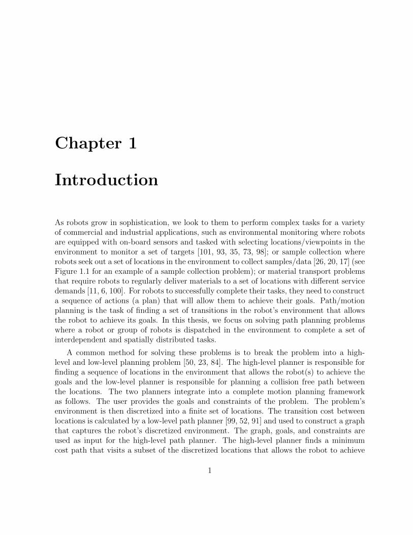
1.1 Robot Operating System (ROS) simulation for a sample collection problem.The left image shows the environment, the layout of the samples, and therobot solution paths. The right image shows the robots returning home aftercollecting one of each mineral type from a subset of the samples. . . . . . 2

3.1 An adder circuit summing up Boolean input variables X = x1, x2, . . . , x5and outputting the Boolean variable b1, as well as the carryout bits. . . . 17

3.2 A-TSP-monotonic example. Interconnecting edges from Gi to Gj shown inthe figure represent a collection of edges that connect every vertex in graphGi to every vertex in graph Gj. The edge weights of the interconnectingedges satisfy the triangle inequality. . . . . . . . . . . . . . . . . . . . . . 31

3.3 On the left is a UAV patrolling example and on the right is a UGV samplecollection example. The robot’s path is indicated with a solid line in bothillustrations and the location marked by an “H” represents the robot’s home.For the patrolling problem, points of interest are buildings represented bylarge squares, faint circles represent the radius that the building can beobserved from, and the grey triangles indicate the different observation per-spectives. In the sample collection problem, the labels above the locationsrepresent the mineral types that are within the sample (large samples havethree minerals and small samples have one). The grey contours representobstacles. . . . . . . . . . . . . . . . . . . . . . . . . . . . . . . . . . . . . 34

3.4 The top plot captures the average normalized solution quality obtained dur-ing the time budget for patrolling instances solved by CBTSP and Gurobi.The bottom plot captures the % of unsolved runs (10 runs per instance)over the time budget. . . . . . . . . . . . . . . . . . . . . . . . . . . . . . 43

xiii

3.5 The top plot captures the average normalized solution quality obtained dur-ing the time budget for sample collection instances solved by CBTSP andGurobi. The bottom plot captures the % of unsolved runs (10 runs perinstance) over the time budget. . . . . . . . . . . . . . . . . . . . . . . . . 45

3.6 A simple period routing example for material transport within a factory.There are only two periods of service and a location can either require servicefor one or both periods (as indicated on the graph). The home location islabelled with an “H”. . . . . . . . . . . . . . . . . . . . . . . . . . . . . . 46

3.7 The top plot captures the average normalized solution quality obtained dur-ing the time budget for period routing instances solved by CBTSP andGurobi. The bottom plot captures the % of unsolved runs (10 runs perinstance) over the time budget. . . . . . . . . . . . . . . . . . . . . . . . . 48

4.1 The results of Γ-Clustering used on an office environment. The red trianglesrepresent locations of interest and the red boxes surround clusters of sizetwo or greater. . . . . . . . . . . . . . . . . . . . . . . . . . . . . . . . . . 51

4.2 This illustration shows three examples of how two clusters can overlap ornot overlap with each other. . . . . . . . . . . . . . . . . . . . . . . . . . 53

4.3 On the left we show an example of clustering in its graph environment withthe edges omitted and on the right we show the same clustering depicted asa forest. . . . . . . . . . . . . . . . . . . . . . . . . . . . . . . . . . . . . . 54

4.4 Path deformation example. . . . . . . . . . . . . . . . . . . . . . . . . . . 70

4.5 Metric example instance (α > β). Vertices in the top row (v2, v3, v5, v6, . . .)are in the cluster Vi. Edge weights connecting vertices within Vi are β. Edgeweights connecting vertices not in Vi are 2α + β. Edge weights connectingvertices not in Vi to vertices in Vi are α + β, unless shown differently indiagram. . . . . . . . . . . . . . . . . . . . . . . . . . . . . . . . . . . . . 71

4.6 A plot showing the tightness of the approximation’s upper bound. The gapbetween the two curves shows where the tightest upper bound can lie. . . 72

4.7 Illustration of how the hierarchical approach progresses. On the left, theprogression of how the path is built. On the right, the levels of nesting inthe clustering are illustrated as a forest (i.e., clusters V4 and V5, as well asvertex 5 are nested in cluster V2). . . . . . . . . . . . . . . . . . . . . . . 81

xiv

4.8 Box plot of the clustering time ratio with respect to the Γ-Clustering ap-proach. The data is categorized by instances that did not time out (Time01)and instances that did time out (Time02). . . . . . . . . . . . . . . . . . . 90

4.9 A plot of the average error for each solver method. Instances are sortedfrom least to most difficult. . . . . . . . . . . . . . . . . . . . . . . . . . . 91

B.1 An adder circuit summing up xc0 , the one-bits of the solution cost. In thisinstance the edges e1, e3, e4, e8, e9 have odd edge weights and all otheredges have even weights. . . . . . . . . . . . . . . . . . . . . . . . . . . . 123

B.2 An example of the widget Ωxi . In this instance the only clauses in F thatcontain the variable xi are clauses c1 and c2. The clause c1 contains theliteral x1 and c2 contains the literal ¬xi. A TSP solution that traverses thewidget from left to right (1 → 9) indicates that xi = 1 in the SAT-TSP

solution and a solution that traverses the widget from right to left (9→ 1)indicates that xi = 0. . . . . . . . . . . . . . . . . . . . . . . . . . . . . . 124

B.3 The connections between widgets in the TSP graph. Dotted edges havezero weight. An edge going into or out of the left of the widget indicates aconnection to left most vertex in the widget chain. Likewise, an edge goinginto or out of the right side indicates a connection to the right most vertexin the chain. . . . . . . . . . . . . . . . . . . . . . . . . . . . . . . . . . . 125

B.4 An illustration of the connections between vertices in a widget and betweenwidgets. In this example the literal xi appears in clauses c1, c2 and c3,the vertices vα, vβ and vγ are short forms for vertices vxi,c1 , vxi,c2 and vxi,c3respectively. The vertices connected with dotted edges have zero edge weightand the solid edges all have the same weight. . . . . . . . . . . . . . . . . 126

B.5 The connections and edge weights between root vertices. If a connection isnot shown, then it does not exist in the GTSP graph. The large arrow fromV ′α to V ′β indicates the connections between the two sets (unidirectional andweighted). The large dotted arrow from V ′β to vxvs indicates the connectionsbetween the two sets (unidirectional with zero edge weights). . . . . . . . 127

xv

B.6 The connection of widget Ωi to Ωj for the reduction of the ordering con-straints. Note that only connections from Ωi to Ωj exist and not the otherway around. Each widget is a copy of the original graph G, of which theedges are represented with dotted lines. The edges connecting vertices fromone widget to another shown with solid lines are only present if the connec-tion exists in G. The edge between vertex vi1 and vj3 highlights how the costmimics the edge weights in G. . . . . . . . . . . . . . . . . . . . . . . . . 133

B.7 The connections between widgets for the reduction of the ordering con-straints. Widgets are connected with directed edges in sequential order. Allwidgets are connected back to the first widget to allow the solution tour toclose. . . . . . . . . . . . . . . . . . . . . . . . . . . . . . . . . . . . . . . 133

B.8 The connections between widgets for the reduction of the multi-robot prob-lem. Widgets are connected with directed edges in sequential order. Allwidgets are connected back to the first widget to allow the solution tour toclose. . . . . . . . . . . . . . . . . . . . . . . . . . . . . . . . . . . . . . . 134

B.9 Performance results for the GTSP approach. The results are broken downinto three categories described in Table B.1. (a) Compares the solver per-formance to the best performance achieved over all approaches. (b) Com-pares the solver performance to the number of additional constraints inGTspLib+. . . . . . . . . . . . . . . . . . . . . . . . . . . . . . . . . . . . 137

B.10 CSP (Gecode) . . . . . . . . . . . . . . . . . . . . . . . . . . . . . . . . . . 138

B.11 Performance results of the CSP approach on the simulation library. Theresults are broken down into three categories described in Table B.1. . . . 138

B.12 Performance results of the BRUTE approach on the full library. Results aredivided into categories described in Table B.1. (a) Compares the solver timeto the best performance achieved over all approaches for SAT-TSP instances.(b) Compares the solver time to the number of SAT-TSP solutions of theinstance. . . . . . . . . . . . . . . . . . . . . . . . . . . . . . . . . . . . . 139

B.13 Performance results of the CBTSP approach on the simulation library. Theresults are broken down into three categories described in Table B.1. (a)Compares the solver time to the best performance achieved over all ap-proaches. (b) Compares the solver time to the number of SAT-TSP solutionsof the instance. . . . . . . . . . . . . . . . . . . . . . . . . . . . . . . . . . 139

xvi

B.14 The number of instances solved by each solver approach. The results arebroken down into four categories described in Table B.2. The number ofmetric and non-metric instances are indicated on the graph with the dottedline and the |M | and |N | symbols respectively. . . . . . . . . . . . . . . . 140

B.15 The number of instances solved in their respective library by each successfulsolver approach. The results are broken down into four categories describedin Table B.2. The number of metric and non-metric instances are indicatedon each graph with the dotted line and the |M | and |N | symbols respectively(there are no non-metric instances in SatLib). . . . . . . . . . . . . . . . 141

B.16 The number of instances solved in their respective library by each successfulsolver approach. The results are broken down into four categories describedin Table B.2. The number of metric and non-metric instances are indicatedon each graph with the dotted line and the |M | and |N | symbols respectively. 142



xvii

Chapter 1

Introduction

As robots grow in sophistication, we look to them to perform complex tasks for a varietyof commercial and industrial applications, such as environmental monitoring where robotsare equipped with on-board sensors and tasked with selecting locations/viewpoints in theenvironment to monitor a set of targets [101, 93, 35, 73, 98]; or sample collection whererobots seek out a set of locations in the environment to collect samples/data [26, 20, 17] (seeFigure 1.1 for an example of a sample collection problem); or material transport problemsthat require robots to regularly deliver materials to a set of locations with different servicedemands [11, 6, 100]. For robots to successfully complete their tasks, they need to constructa sequence of actions (a plan) that will allow them to achieve their goals. Path/motionplanning is the task of finding a set of transitions in the robot’s environment that allowsthe robot to achieve its goals. In this thesis, we focus on solving path planning problemswhere a robot or group of robots is dispatched in the environment to complete a set ofinterdependent and spatially distributed tasks.

A common method for solving these problems is to break the problem into a high-level and low-level planning problem [50, 23, 84]. The high-level planner is responsible forfinding a sequence of locations in the environment that allows the robot(s) to achieve thegoals and the low-level planner is responsible for planning a collision free path betweenthe locations. The two planners integrate into a complete motion planning frameworkas follows. The user provides the goals and constraints of the problem. The problem’senvironment is then discretized into a finite set of locations. The transition cost betweenlocations is calculated by a low-level path planner [99, 52, 91] and used to construct a graphthat captures the robot’s discretized environment. The graph, goals, and constraints areused as input for the high-level path planner. The high-level planner finds a minimumcost path that visits a subset of the discretized locations that allows the robot to achieve

1

Figure 1.1: Robot Operating System (ROS) simulation for a sample collection problem.The left image shows the environment, the layout of the samples, and the robot solutionpaths. The right image shows the robots returning home after collecting one of each mineraltype from a subset of the samples.

the goals, while obeying the constraints of the problem. The high-level path is then givento the low-level planner which finds a collision free path in the continuous space betweenthe high-level locations. The complete solution allows the robot(s) to move in the physicalworld, achieve the goals, and obey the constraints while approximating optimal solutionpaths (the discretization may eliminate optimal solutions). Note, a more general versionof this framework transitions between robot states, instead of robot locations. Adoptingthis strategy allows us to simplify a large path planning problem with a high density ofinformation into one problem with sparse information (the high-level problem) and a seriesof small problems with dense information (the low-level problems). This thesis addressesthe problem of solving high-level path planning problems where obstacle avoidance androbot to robot collisions are handled by the low-level planner. This thesis also refers tohigh-level problems as discrete path planning problems.

Many discrete path planning problems tend to have a strong combinatorial aspect tothem and thus, many of these problems are intractable (NP-hard) [94]. This means thetask of finding an optimal solution path, is the task of searching an exponentially largespace, for which there is no known efficient method. There are a number of good solversthat we can use to search this space [32, 66, 12]. However, to utilize these solvers, we wouldneed to express the path planning problem in a form readable by the solver. A commonchoice, is to use a mathematical solver which requires us to express the path planning

2

problem as an integer linear program (ILP). Mathematical solvers have received a lot ofacademic and commercial attention, as such they tend to be high performers that use anumber of sophisticated techniques, some of which are proprietary and thus hidden fromthe public.

1.1 Literature Survey

In this section we give an overview of the literature related to solving high-level pathplanning problems. In subsequent chapters we provide a more in depth review of theliterature related to the chapter’s topic.

There is a set of specialized discrete path planning problems that have purpose builtsolvers. Two such examples of problems with purpose built solvers are the travellingsalesman problem (TSP) and its generalized version, GTSP. TSP looks to find shortesttours visiting the locations and GTSP looks to find shortest tours that visit one location ineach set of locations (the sets are provided as input). These problems appear in a varietyof applications. In [10] and [17], the authors use TSP to find coverage paths for theirenvironments. In [81], the authors use GTSP to find minimum length paths for a roboticwelding arm. In [64], the authors use GTSP to find paths that monitor the environment.There are some very good solvers for both of these problems such as Concorde [3], LKH [32],GLKH [33] and GLNS [88]. To take advantage of the years of research that has wentinto these solvers, the user would need to translate their path planning problem to thespecialized problem. However, due to the specialized nature of these problems the usermay find this translation task challenging.

As stated, ILP [67] is a general framework used for modelling path planning problems.There are a number of good solvers, for which CPLEX [1] and Gurobi [66] are two ofthe more popular commercial solvers and SCIP [2] is one of the fastest non-commercialsolver. In [68], the authors use MILP to plan optimal trajectories, and in [56, 44] ILP isused to solve multi-robot charging problems. In [102], the authors give an ILP solution forcollision-free multi-robot problems.

Another common framework for expressing path planning problems is LTL. Here theuser models their problem with a set of state transitions, e.g., if the robot is at location xthen the next location it will visit is y. Solvers developed in the model checking communitycan be used to compute runs (expressed as an automaton) that satisfy the LTL formula [36,12]. In [89], LTL is used to express a class of persistent patrolling problems and the authorspropose a method for computing optimal plans rather than just feasible plans. In [48], LTLis used to express multi-robot planning problems.

3

The STRIPS problem specification language [24] and its successor, PDDL [25] are likeLTL in that the user models their problem as a set of state transitions (PDDL’s transitionsare more expressive than LTL). An annual competition [95] is held to encourage partici-pants to develop better solvers. The problems in the competition range from emergencyresponse scenarios to making a sandwich. There are a number of good solvers for theseexpressions such as FF [34] and LAMA [78].

1.2 Contributions

This thesis looks to solve high-level path planning problems. Below we give the contribu-tions and organization for this thesis.

Chapter 2 Reviews the concepts needed to solve high-level path planning problems andsolves an example problem with the ILP approach.

Chapter 3 This chapter introduces a novel alternative to ILP, called SAT-TSP. Wedesigned SAT-TSP as a modelling language for expressing path planning problems. Thelanguage is structured in such a way to allow us to leverage recent techniques for Sat-isfiability Modulo Theory (SMT). We provide the SMT based solver CBTSP, for solvingdiscrete path planning problems expressed as SAT-TSP problems. We prove its correctnessand benchmark it against a commercial-grade ILP solver on a set of three important mo-tion planning problems: patrolling, sample collection with multiple robots, and periodicrouting. Our results show that CBTSP outperforms the ILP solver on a majority of theinstances, especially the more difficult to solve problems.

In Appendix B we provide five additional SAT-TSP solvers and benchmark them againstCBTSP. These alternatives were not as successful as CBTSP and are therefore omitted fromthe main body of this thesis.

Additionally, we provide a demo video1 depicted in Figure 1.1 demonstrating one ofour application problems in a ROS environment with Husky robots.

The work presented in this chapter is based on the following publications:

• Frank Imeson and Stephen L Smith. A language for robot path planning in discreteenvironments: The TSP with Boolean satisfiability constraints. In IEEE Interna-tional Conference on Robotics and Automation, pages 5772–5777, 2014.

1https://ece.uwaterloo.ca/~sl2smith/SAT-TSP/demo.mp4

4

https://ece.uwaterloo.ca/~sl2smith/SAT-TSP/demo.mp4

• Frank Imeson and Stephen L Smith. Multi-robot task planning and sequencingusing the SAT-TSP language. In IEEE International Conference on Robotics andAutomation, pages 5397–5402, 2015.

• Frank Imeson and Stephen L Smith. An SMT-based approach to motion planningfor multiple robots with complex constraints. IEEE Transactions on Robotics (inreview).

Chapter 4 This chapter introduces a new technique for improving the efficiency of ex-isting path planning solvers. The chapter introduces the clustering method Γ-Clustering,that it uses to prune off large portions of the solution search space (to improve solverefficiency). It provides an efficient algorithm for computing the optimal Γ-Clustering. Thechapter also provides two path planning solver approaches for pruning the solution space.The first path planning solver approach, coupled planning, reduces the solution search spaceby restricting how feasible paths visit the Γ-Clusters. The second approach, hierarchicalplanning, further reduces the search space by decomposing the problem into a hierarchyof independent problems. This additional reduction of search space is at the expense ofsolution quality. However, in the chapter we prove that both methods find solutions withina constant factor of the optimal.

Our benchmark compares the two solver approaches to the standard approach withoutclustering. All simulations use an ILP solver to find path planning solutions. The bench-mark problems consist of TSP, sample collection, and period routing problems. The resultsshow that the coupled method and the hierarchical method find high quality solutions, typ-ically within 10% of optimal. The results also show that as the problems become moredifficult to solve, the coupled approach is able to maintain its performance longer than thestandard approach, and the hierarchical approach is able to maintain its performance evenlonger.

Additionally, we compare the quality Γ-Clusters to the quality of clusters found by sixdifferent clustering methods. The benchmark shows that overall the quality of Γ-Clustersis superior to those found by the other methods.

The work presented in this chapter is based on the following publications:

• Frank Imeson and Stephen L Smith. Clustering in discrete path planning for approx-imating minimum length paths. In American Control Conference, pages 2968–2973,Seattle, WA, May 2017.

5

• Frank Imeson and Stephen L Smith. A hierarchical decomposition for computingapproximate solutions to vehicle routing problems. Submitted to International Con-ference on Automated Planning and Scheduling (ICAPS), 2018.

Chapter 5 This chapter summarizes the work presented in this thesis and presents thefuture directions this work could take.

Other Publications I have also collaborated on an article that introduces a new solverfor the generalized travelling salesman problem (GTSP). However, this work is not pre-sented in this thesis.

• Stephen L Smith and Frank Imeson. GLNS: An effective large neighborhood searchheuristic for the generalized traveling salesman problem. Computers & OperationsResearch, 2017.

6

Chapter 2

Preliminaries

This chapter reviews the concepts needed for solving high-level path planning problems.We walk the reader through each step of the process, starting with graphs.

2.1 Graphs

Graphs are used to represent the robot’s discrete environment. The vertices in the graphrepresent the locations in the robot’s environment and the set of edges capture the allowabletransitions between the locations the robot is able to make. For example, an edge 〈A,B〉with weight w(A,B) = 4 tells us that the robot may transition from location A to locationB and if it does so then it will incur a cost of 4 (this cost may represent the time, distance,etc., that the robot incurs to make the transition).

A graph G is defined by its tuple 〈V,E,w〉, where V is the set of vertices, E is the setof edges, and w maps an edge 〈va, vb〉 ∈ E to its weight/cost. In this thesis we do not allownegative weight edge transitions.

A complete graph contains an edge for every possible transition — there is an edge fromevery vertex to every other vertex (|E| = |V |2). An undirected graph has edges that areused to capture transitions between locations, e.g., an edge 〈A,B〉 describes the transitionfrom A to B and B to A. This is not the case for directed graphs, where an edge is requiredto capture the transition from a location A to a location B and a separate edge is requiredto capture the transition from B to A. Directed graphs allow for a greater expression ofinformation and thus complexity (e.g., we can express one-way transitions). In this thesis,the assumption is that graphs are directed.

7

A metric graph is a complete graph that satisfies the triangle inequality. Formally, thetriangle inequality states that for every set of vertices A,B,C ∈ V the following holds:

w(A,C) ≤ w(A,B) + w(B,C).

Many robotic environments satisfy the triangle inequality and thus their graph’s are metric.

We use graphs to plan a sequence of transitions from one vertex to the next, whichallows us to navigate the robot in its environment. We refer to these sequences as paths.In this thesis we concentrate on paths and cycles of the following form.

Definition 2.1.1 (Paths and Cycles). Given a graph G = 〈V,E,w〉, we define a path asa non-repeating sequence of vertices in V , connected by edges in E. A cycle is a path inwhich the first and last vertex are equal.

A Hamiltonian path is a path that visits every vertex in V (exactly once) and a Hamil-tonian cycle is a cycle that visits every vertex in V (exactly once).

A path p can also be represented by the set of edges it traverses. The cost c of the pathp is the sum of its transition costs:

c =∑

〈va,vb〉∈p

w(va, vb).

2.2 The Travelling Salesman Problem

The travelling salesman problem (TSP) is one of the most studied vehicle routing prob-lems [4]. This chapter uses the TSP to demonstrate how to solve high-level path planningproblems. Traditionally the TSP problem is posed as a salesman wanting to find a mini-mum length tour that visits a set of cities, where the length of the tour represents the totaldistance travelled.

Problem 2.2.1 (Travelling Salesman Problem). Given a complete and weighted graphG = 〈V,E,w〉, find a Hamiltonian cycle of G with minimum cost.

2.3 Complexity Theory

Understanding the problem’s complexity, is key to understanding the computational effortneed to solve the problem. This will help us chose which solver approach to use. For

8

example, some problems can be solved in a polynomial amount time and thus one wouldlikely want to choose a solver approach that guarantees the solution is found in a polynomialamount time.

2.3.1 Decision Problems

Many high-level path planning problems are optimization problems that look to find thelowest cost solution(s). Decision problems on the other hand are problems with a yes or ano answer. The decision version of the optimization problems that we are interested in areas follows: is there a solution to the problem of cost c or lower. For example, the decisionversion of TSP looks to find Hamiltonian cycle of cost c or less. In this way we can betterclassify the complexity of finding solutions, not just finding optimal solutions.

2.3.2 Complexity Classes

The study of complexity theory has discovered that there is a set of classes that we can useto classify a problem’s complexity. These classes allow us to formally detect if problem Ais a variant of problem B, thus allowing us to use techniques/solvers developed for problemB on problem A. This is done by reducing problem A to problem B and solving it withproblem B’s solver. The algorithm used for the reduction must run in a polynomial amountof time, otherwise it is arguably a misuse of computational effort that could instead beused to find solutions for problem A.

Problem A is said to be complete in its complexity class if any other problem B in thesame complexity class can be efficiently reduced to A. A problem is said to be hard forsome complexity class X if it is at least as hard as the hardest problem in X (it can beharder than all of the problems in X). A problem instance is a specific realization of theproblem. For example, if we were given a graph G with 10 vertices and we wished to finda shortest tour visiting each vertex exactly once, then the graph G is the instance and theproblem is a TSP problem.

The complexity class NP captures the set of problems that have solutions that areefficiently verifiable. For example, a problem A is in NP if given a solution to a probleminstance of size n, then we can verify the solution with a polynomial amount of time(O(nb), where b is some constant). Problem A is NP-hard if it is as hard or harder thanany problem in NP. Thus NP-complete problems are NP-hard.

As an example, the decision version of TSP problem is NP-complete— given a graphG, a tour p, and a budget c we can efficiently verify that the path p has cost c or less. The

9

optimization version of TSP is NP-hard, as one cannot efficiently verify that a solutionp is the lowest cost solution. Therefore, to solve TSP problems we will look for a solverapproach that can handle problems in this complexity class.

Some additional complexity classes are: the class P, which capture all problems thatare solvable in polynomial time with respect to the input size of the problem; the classPSpace, which capture problems that are solvable with a polynomial amount of space;and the class EXPSpace, which are problems solvable with an exponential amount ofspace. The class P is a subset of NP and it is believed that it may be a strict subset. Weprovide the following relations to understand which classes are contained within each otherand thus work towards understanding which problems are harder to solve than others:

P ⊆ NP ⊆ PSpace ⊆ EXPSpace.

2.4 Using ILP to Find Solution Paths

As stated, integer linear programming is a good general approach for finding solutions forhigh-level path planning. This approach is suitable for finding optimal solutions for pathplanning problems that have their decision problem in the class NP-complete.

This approach uses a series of linear inequalities coupled with an objective to model theplanning problem. The inequalities capture relationships between the variables, which canonly take on integer values and the objective is a linear equation that is to be minimized(or maximized). The solver attempts to find an optimal assignment of the variables thatsatisfies the set of inequalities (minimize the objective).

Now we walk the user through how to solve TSP problems with an ILP solver. Let ususe the set of variables ei,j|〈vi, vj〉 ∈ E to represent the edges and the set of variablesvi ∈ V to represent the set of vertices for the ILP expression.

10

minimize ∑vi∈V

∑vj∈V \vi

ei,jw(vi, vj) (2.1)

subject to ∑vj∈V \vi

ei,j = 1, for each vi ∈ V (2.2)

∑vi∈V \vj

ei,j = 1, for each vj ∈ V (2.3)

∑vi,vj∈S

ei,j ≤ |S| − 1, for each S ⊂ V s.t. |S| ≥ 2 (2.4)

0 ≤ vi ≤ 1, for each vi ∈ V (2.5)

0 ≤ ei,j ≤ 1, for each 〈vi, vj〉 ∈ E (2.6)

The above formulation was taken from [70]. The objective (2.1) captures the cost ofthe solution by adding all the edge weights that are included in the tour. Constraints (2.2)and (2.3) ensure that there are exactly one incoming and one outgoing edge for each vertex.Then subtours (a solution with multiple tours instead of one tour) are eliminated in Con-straint (2.4) by explicitly eliminating every possible tour. There are an exponential numberof these constraints and so in practice these constraints are added to the formulation asthe solver violates them. This is referred to as a lazy constraint.

Once the ILP solver has found a solution, we translate it back to a TSP solution. Thisis trivially done for this example since the set of edges that construct the tour p are theset of included edge variables in the ILP solution.

Remark 2.4.1. We chose the above ILP expression over a polynomial expression because ofits effectiveness. The decision version of TSP is NP-complete, thus there are polynomialtime reductions to ILP such as the MTZ formulation [57], however in practice, betterperformance is achieved with the above expression [70, 69].

2.5 Summary

In this chapter we reviewed the steps for solving high-level path planning problems usingan ILP approach. A summary of the steps are as follows:

11

1. Classify the path planning problem’s complexity.

2. Choose an approach capable of solving problems of said complexity (for our example,we used ILP).

3. Express the problem in a readable format for the chosen approach.

4. Use an exiting solver to find solution(s).

In the next chapter we explore an alternative approach to ILP, then in Chapter 4 weexplore two methods for improving solver efficiency (the chapter improves the efficiency ofan ILP solver).

12

Chapter 3

An Alternative to ILP

In this chapter we propose an alternative to the ILP approach for solving high-level pathplanning problems. We focus on the class of problems that require the allocation of tasksto robots and a set of efficient paths that allow the robots to visit their task locations.

We start by introducing the new problem language SAT-TSP. We use this language toexpress/model high-level path planning problems. The problem is a combination of thesatisfiability problem (SAT) and the travelling salesman problem (TSP). The SAT problemtakes in as input a Boolean formula and asks the question is there an assignment of thevariables that satisfies the formula. The TSP problem takes in as input a graph and searchesfor the minimum cost Hamiltonian cycle (see Section 2.2). The SAT-TSP problem takesin as input: one formula, one or more graphs (multiple robots use multiple graphs), andone or more cost budgets (multiple robots may use multiple cost budgets). We use theformula to express the problem’s constraints and the graphs and cost budgets are usedto capture the sequencing/routing problems. The constraints and the environment(s) arelinked together via a set of variables. Here a location in the environment is visited ifand only if its corresponding variable is assigned true. This allows SAT-TSP to expresslogical constraints on the robots’ motion, such as task dependencies, incompatibilities, andcapacity constraints. A SAT-TSP solution is a set of paths (one for each robot) that visitsa subset of locations in the environment, satisfies the constraints, and has transitions thatare within the cost budget(s).

The structure of SAT-TSP allows us to leverage recent developments in the SatisfiabilityModulo Theory (SMT) community. Specifically, we developed the solver CBTSP to solveSAT-TSP problems using the SMT framework. In this way we were able to combine astate-of-the-art SAT solver with a state-of-the-art TSP solver.

13

The SAT-TSP problem inherits the strengths of its sub-problems, SAT and TSP. As suchit is most suited for path planning problems with constraints that are efficiently expressibleas SAT formulae and optimization objectives resembling shortest paths/tours. Converselyif a set of problems contain constraints that are not efficiently expressible in SAT or theproblem has an optimization objective that has nothing to do with the robots transitions,then SAT-TSP would likely be a poor choice.

The contributions of this chapter are as follows. We formally introduce the SAT-TSP

problem language and characterize its complexity. Specifically, we show that even whenSAT-TSP is compromised of easy SAT and TSP problems, the SAT-TSP instance can stillbe hard. We provide the SAT-TSP solver, CBTSP, and prove its correctness. Then webenchmark CBTSP against an ILP approach on a series of high-level path planning prob-lems: patrolling problems, multi robot sample collection problems, and periodic routingproblems. The results show that CBTSP often outperforms the ILP approach — especiallyon more difficult instances.

This chapter is organized as follows. Section 3.1 reviews the related work to theSAT-TSP approach. Section 3.2 provides the necessary background needed for this chapter.Section 3.3 formally introduces the SAT-TSP problem and classifies its complexity. Sec-tion 3.4 introduces the CBTSP solver, proves its correctness for the class of TSP-monotonicinstances (Definition 3.4.2), and provides a relaxation for the TSP-monotonic class to ex-pand the set of solvable instances. Section 3.5 outlines the ILP approach used for ourcomparison and Section 3.6 shows how to express patrolling, collection, and period rout-ing problems with SAT-TSP and ILP. Section 3.7 details our benchmark and presents theresults. For the interested reader we provide five additional SAT-TSP solver approaches inAppendix B, which consist of SAT, TSP, GTSP, CSP, and SMT solver approaches.

3.1 Related Work

This section builds upon Section 1.1 to provide a more in depth review of the literaturerelated to this chapter. As previously stated, TSP, GTSP, ILP, LTL, and STRIPS are allgeneral frameworks used for solving high-level path planning problems.

The TSP and GTSP problems are more specialized than the SAT-TSP problem. As such,using TSP or GTSP to model complex path planning problems is more challenging thanusing SAT-TSP. TSP and GTSP solvers are geared towards searching for low cost paths —not solving complex logic. This is in contrast with SAT solvers, which are geared towardsusing the logic of the problem to eliminate infeasible solutions. As such there is no reason

14

to believe that TSP and GTSP solvers would be proficient at solving complex path planningconstraints. Regardless, in Appendix B we explore using TSP and GTSP solvers for findingSAT-TSP solutions.

The non-optimization version (the decision version) of ILP, like SAT-TSP isNP-complete— both can express the same set of problems. However, in practice bothapproaches have their own limitations. For example, unlike ILP, it is arguably awkwardto use SAT-TSP for counting constraints (e.g., visit x red locations). This is due to thesimple structure that SAT uses for expressing logic. However, this structure has led to thesuccess of the DPLL [19, 18] and DPLL(T) [63] algorithms, which are used in modern SATsolvers [90, 59] and CBTSP. Furthermore, we demonstrate in this chapter that SAT-TSP canbe successfully used for counting constraints. We provide a direct comparison of CBTSP

to the commercial ILP solver, Gurobi, on a set of robotic path planning problems and theresults show that CBTSP often outperforms the ILP solver.

Many important path planning problems lie in NP and our goal in this chapter isto produce a solver that is tailored to problems in this class. A drawback of LTL, isthat LTL is in a higher complexity than SAT-TSP. Specifically, the decision version ofLTL is in the class PSpace-complete [87] where the decision version of SAT-TSP is in theclass NP-complete. The LTL language is likely more expressive than SAT-TSP, since it isbelieved that PSpace is a strict superset of NP. For example, LTL can be used to expressplanning problems that consist of infinite length solution paths (i.e., persistent problems)where SAT-TSP cannot. There are potential downfalls of using a more complex language,such as allowing the user to inadvertently increase the complexity of their problem. Forexample suppose the user requires a path from location A to location B (any path) andthe user has access to a TSP solver. If they choose to express their problem as a TSP, theywould be able to find a solution to their problem but they would have also increased thecomplexity of their problem.

STRIPS and PDDL are capable of expressing problems in EXPSpace [21], which isbelieved to be a strict superset of PSpace and thus NP. This work focuses on problemsin NP and uses an integer programming approach as our point of comparison.

Our main solver, CBTSP is based on SMT which is an extension of SAT that allowsfor first order logic. SMT solvers have previously been proposed for solving path planningproblems. In [86] and [38], the authors solve the high-level and low-level path planningproblems simultaneously. This is unlike our approach where we leverage the SMT frame-work to better solve the high-level problem. In [60] and [80], the authors use an off the shelfSMT solver to find solutions for the high-level path planning problem. Our approach differsfrom these by using a custom SMT theory that specializes in handling the combinatorial

15

nature of sequencing locations. Additionally, we have explored solving SAT-TSP instanceswith an SMT solver and found that it does not scale well (the results are provided in Ap-pendix B). To the best of our knowledge, we are the first to solve high-level path planningproblems using a custom SMT theory to handle the combinatorial aspect of sequencing.

3.2 Background

This section reviews the background concepts needed for this chapter.

3.2.1 Boolean Satisfiability (SAT)

In this chapter we use the Boolean satisfiability problem (SAT) [18] to encode path planningconstraints. A SAT formula is a propositional formula that is composed of Boolean literalsand operators. A literal is either a Boolean variable (x) or its negation (¬x). The operatorsare conjunction (∧, and), disjunction (∨, or) and negation (¬, not), which may operateon the literals or other Boolean formulae. An assignment of the variables (true or false)results in the formula being satisfied (true) or not (false). The conjunctive normal form(CNF-SAT) is the canonical form of SAT. A formula F is in its canonical form if the formulais a conjunction of clauses, where each clause is a disjunction of literals. We allow formulasto be expressed in non-canonical form.

Problem 3.2.1 (SAT). Given a propositional Boolean formula F , determine if it is satis-fiable.

3.2.2 Boolean Circuits

Developing SAT expressions to capture constraint logic can be difficult. To aid in thisprocess, one can borrow from Boolean circuits. In this chapter we borrow logic from addercircuits to construct counting constraints.

Adder circuits are used in electronics to do rudimentary mathematical operations [55].Given an input set X of Boolean signals, the adder circuit counts the number of signalsthat are true (high). The example circuit shown in Figure 3.1 takes as input, a set ofsignals X = x1, x2, . . . , x5 and outputs the bit b1. This circuit is composed of four twobit adder circuits. The circuit constrains the binary one bit b1 to the equal the numberof true input variables in X. There would be a similar circuit for the twos bit that takes

16

These carry over bits are used as inputin the next level of adder circuit.

XOR gate.

AND gate.

2-Bit Adder circuits

Figure 3.1: An adder circuit summing up Boolean input variables X = x1, x2, . . . , x5and outputting the Boolean variable b1, as well as the carryout bits.

in as input, all of the carry out bits from the example. The complete binary circuit isconstructed using techniques in [55]. The circuit is then translated to a Boolean formula(SAT) in polynomial time using methods from [41].

3.2.3 SMT and DPLL(T)

Satisfiability Modulo Theory (SMT) is an extension of SAT that allows for first-order logic.The SMT framework extends SAT by linking non-SAT theories back to the SAT formula.Specifically, the SMT problem uses a propositional formula F defined over a set of Booleanvariables X that contain a set of predicate variables xt ∈ XT for each theory instancet ∈ T . Each theory instance belongs to a specialization of decidable first-order logic, suchas arithmetic logic or quantifiable Boolean logic. The power of this approach is that a SATsolver can be used to solve the propositional formula while a set of specialized solvers canbe used for the theories.

Definition 3.2.2 (SMT). An SMT formulation 〈F, T 〉, is satisfiable if and only if

1. F is a propositional formula defined over X ⊇ XT ,

2. T is a set of decidable first-order logic problems defined over Q such that X ⊆ Q,

3. and there exists an assignment of Q satisfying F such that for every t ∈ T thecorresponding predicate variable xt agrees with the evaluation of xt (true or false).

17

DPLL(T): The DPLL(T) algorithm for solving SMT instances is based on the DPLLalgorithm [18] using solving SAT instances (propositional formulae). The DPLL algorithmsolves F by building a list of assignments for the Boolean variables in F (a partial solution).This algorithm extends DPLL to incorporate theories by linking the predicates xt ∈ X tothe theories t ∈ T . Informally, the algorithm works as follows: as partial solutions forF are being constructed by the DPLL algorithm, the theory solvers are called to confirmthat the partial SAT solutions are consistent with the theories. If a theory is consistent,then the DPLL algorithm continues. If not, the theory solver that detected the conflictconstructs a learnt clause fconflict to capture the conflict over the set Boolean variables X.The learnt clause is added to F ← F ∧ fconflict and the algorithm backtracks some or all ofits assignments until the partial solution no longer conflicts with the new F .

Note 3.2.3. The above description of DPLL(T) captures only the mechanisms of DPLL(T)that are utilized by the CBTSP solver. A full description of DPLL(T) can be found in [63].

3.2.4 Induced Subgraphs

An induced subgraph is a subgraph of G that contains a subset of the vertices and all theedges connected to those vertices.

Definition 3.2.4 (Induced Subgraph). The induced subgraph of a graph G = 〈V,E,w〉 forV ′ ⊆ V is the graph G′ = 〈V ′, E ′, w〉 with E ′ = 〈vi, vj〉 ∈ E|vi, vj ∈ V ′. We say that G′

is induced by V ′.

3.3 Problem Statement

In this section we provide a formal definition of the SAT-TSP problem and classify itscomplexity.

3.3.1 SAT-TSP Definition

Before we define the decision version of SAT-TSP and its two optimization problems, westart with some notation. A SAT-TSP instance can take as input multiple graphs with acost budget ci for each input graph Gi. To simplify the notation we sometimes absorb thecost budget ci into the graph’s tuple Gi = 〈Vi, Ei, wi, ci〉 (when there is only one graph, wedo not absorb the cost budget). A formula F has a solution or partial solution M , which

18

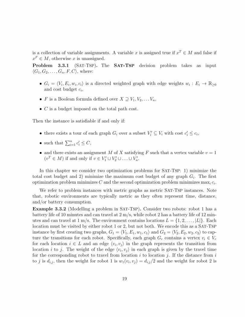
is a collection of variable assignments. A variable x is assigned true if xT ∈M and false ifxF ∈M , otherwise x is unassigned.

Problem 3.3.1 (SAT-TSP). The SAT-TSP decision problem takes as input〈G1, G2, . . . , Gn, F, C〉, where:

• Gi = 〈Vi, Ei, wi, ci〉 is a directed weighted graph with edge weights wi : Ei → R≥0

and cost budget ci,

• F is a Boolean formula defined over X ⊇ V1, V2, . . . Vn,

• C is a budget imposed on the total path cost.

Then the instance is satisfiable if and only if:

• there exists a tour of each graph Gi over a subset V ′i ⊆ Vi with cost c′i ≤ ci,

• such that∑n

i=1 c′i ≤ C,

• and there exists an assignment M of X satisfying F such that a vertex variable v = 1(vT ∈M) if and only if v ∈ V ′1 ∪ V ′2 ∪ . . . ∪ V ′n.

In this chapter we consider two optimization problems for SAT-TSP: 1) minimize thetotal cost budget and 2) minimize the maximum cost budget of any graph Gi. The firstoptimization problem minimizes C and the second optimization problem minimizes maxi ci.

We refer to problem instances with metric graphs as metric SAT-TSP instances. Notethat, robotic environments are typically metric as they often represent time, distance,and/or battery consumption.

Example 3.3.2 (Modelling a problem in SAT-TSP). Consider two robots: robot 1 has abattery life of 10 minutes and can travel at 2 m/s, while robot 2 has a battery life of 12 min-utes and can travel at 1 m/s. The environment contains locations L = 1, 2, . . . , |L|. Eachlocation must be visited by either robot 1 or 2, but not both. We encode this as a SAT-TSP

instance by first creating two graphs, G1 = 〈V1, E1, w1, c1〉 and G2 = 〈V2, E2, w2, c2〉 to cap-ture the transitions for each robot. Specifically, each graph Gr contains a vertex vi ∈ Vrfor each location i ∈ L and an edge 〈vi, vj〉 in the graph represents the transition fromlocation i to j. The weight of the edge 〈vi, vj〉 in each graph is given by the travel timefor the corresponding robot to travel from location i to location j. If the distance from ito j is di,j, then the weight for robot 1 is w1(vi, vj) = di,j/2 and the weight for robot 2 is

19

w2(vi, vj) = di,j. Now the tuple 〈V1, E1, w1, 10〉 captures the transition system for robot 1and its battery budget, similarly tuple 〈V2, E2, w2, 12〉 for robot 2.

Next we construct the formula F using the set of variables X = vi,r|i ∈ L, r ∈ R thatrepresents if vertex vi ∈ Gr is in the solution or not (true or false). We start by adding theset of clauses (vi,1 ∨ vi,2) to F for each i ∈ L, to express that each location i ∈ L must bevisited by at least one robot. Then we add the clauses (¬vi,1 ∨ ¬vi,2) to express that eachlocation i ∈ L can be visited by at most one robot.

Finally, we choose a value for the total cost budget, to be any value C ≥ 22, since anysolution satisfying the individual robot budgets will also satisfy this C. If we wish to findthe solution with the lowest total cost, we search for feasible solutions that minimize C.

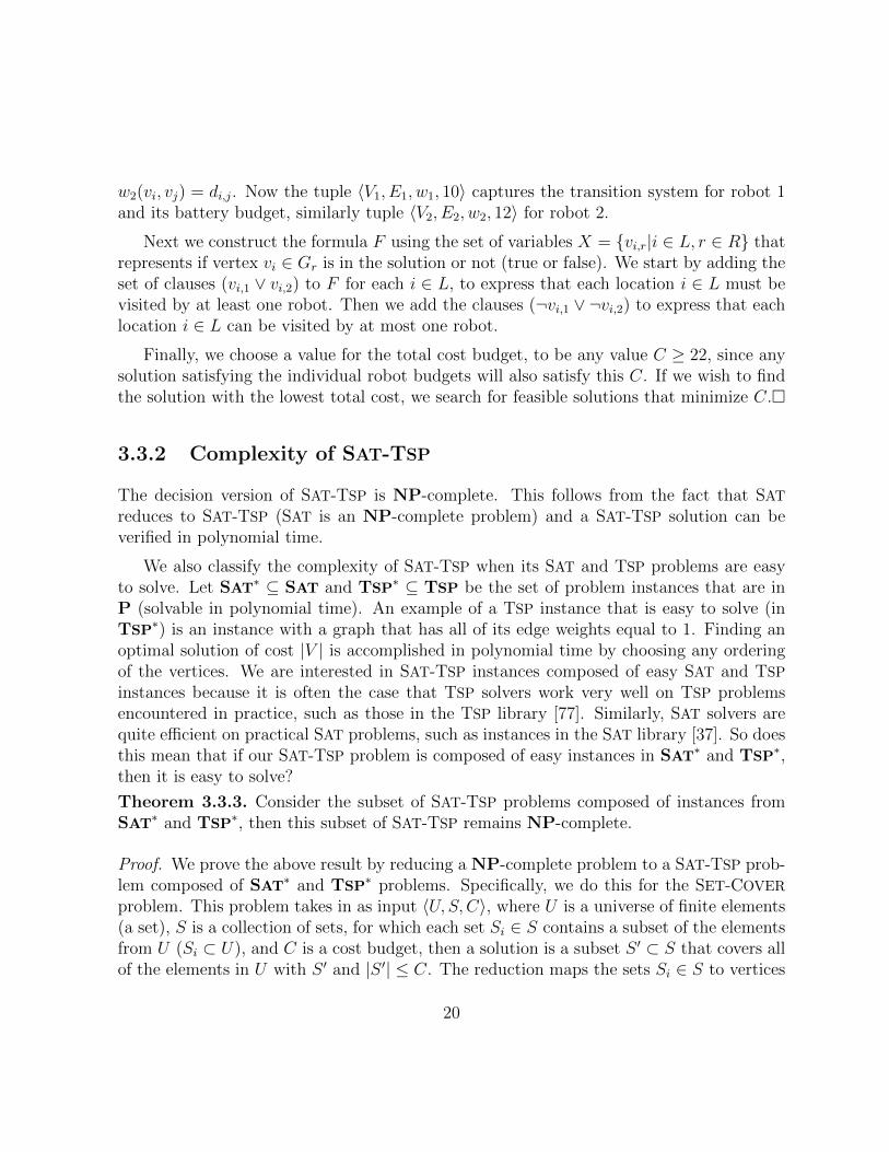
3.3.2 Complexity of SAT-TSP

The decision version of SAT-TSP is NP-complete. This follows from the fact that SATreduces to SAT-TSP (SAT is an NP-complete problem) and a SAT-TSP solution can beverified in polynomial time.

We also classify the complexity of SAT-TSP when its SAT and TSP problems are easyto solve. Let SAT

∗ ⊆ SAT and TSP∗ ⊆ TSP be the set of problem instances that are in

P (solvable in polynomial time). An example of a TSP instance that is easy to solve (inTSP

∗) is an instance with a graph that has all of its edge weights equal to 1. Finding anoptimal solution of cost |V | is accomplished in polynomial time by choosing any orderingof the vertices. We are interested in SAT-TSP instances composed of easy SAT and TSP

instances because it is often the case that TSP solvers work very well on TSP problemsencountered in practice, such as those in the TSP library [77]. Similarly, SAT solvers arequite efficient on practical SAT problems, such as instances in the SAT library [37]. So doesthis mean that if our SAT-TSP problem is composed of easy instances in SAT

∗ and TSP∗,

then it is easy to solve?

Theorem 3.3.3. Consider the subset of SAT-TSP problems composed of instances fromSAT

∗ and TSP∗, then this subset of SAT-TSP remains NP-complete.

Proof. We prove the above result by reducing a NP-complete problem to a SAT-TSP prob-lem composed of SAT

∗ and TSP∗ problems. Specifically, we do this for the SET-COVER

problem. This problem takes in as input 〈U, S, C〉, where U is a universe of finite elements(a set), S is a collection of sets, for which each set Si ∈ S contains a subset of the elementsfrom U (Si ⊂ U), and C is a cost budget, then a solution is a subset S ′ ⊂ S that covers allof the elements in U with S ′ and |S ′| ≤ C. The reduction maps the sets Si ∈ S to vertices

20

vi in the complete graph G = 〈V,E,w〉, where the edges in the graph all have a weight of1. The inclusion/exclusion of a set Si is indicated by the SAT-TSP tour visiting the vertexv′i ∈ V . The SAT-TSP formula

F =∧uj∈U

∨i|uj∈Si

vi

is used to ensure that each element uj ∈ U is covered by at least one set Si. A solution tothe SAT-TSP problem 〈G,F,C〉 (C is given as input to the set cover problem) is a tour oflength c′ ≤ C, which translates to a set cover solution with c′ sets (|S ′| = c′).

The TSP instance G and sub-instances have the trivial solution of any tour (all tourshave the same cost since all edges have weight 1). The SAT instance F and sub-instancesalso have trivial solutions since there are no negative literals in the formula (we simplyassign all the literals to be true). Thus, both the SAT and TSP instances are solved inlinear time (polynomial time) and since SET-COVER is NP-hard, then it must be the casethat SAT-TSP remains NP-complete despite the fact that the SAT and TSP problems arein SAT

∗ and TSP∗ respectively.

Theorem 3.3.3 proves that SAT-TSP is NP-hard even when its sub-problems are easy.Therefore, we expect that an effective SAT-TSP solver will require some additional level ofsophistication on top of being able to solve SAT and TSP problems.

The next Section starts by introducing the BRUTE solver as a naıve combination of aSAT and TSP solver that explores every SAT solution (there may be exponential numberof solutions to explore). The CBTSP solver improves upon BRUTE by adding the abilityto negate partial solutions while leveraging the sophistication of the SAT solver to choosecandidate solutions. This ability of negating partial solutions allows CBTSP to more effec-tively prune the search space. Letting the SAT solver choose the candidate solutions allowsus to take advantage the algorithm’s ability to find the variables/locations in the problemthat cause the most conflicts.

3.4 CBTSP: An SMT-based approach for SAT-TSP

In this section we provide a simple BRUTE solver as a lead-in to the CBTSP solver. Weprovide a high-level description of the CBTSP solver and provide the conditions under whichCBTSP can be used.

21

3.4.1 The BRUTE Approach: A Lead-in to CBTSP

The BRUTE approach decouples the SAT-TSP instance by first solving the SAT instanceand then the TSP instance. For simplicity, Algorithm 1 implements a SAT-TSP solverthat only takes instances with one input graph. The algorithm is easily extended to takemultiple graphs by replacing Line 5 with multiple calls to the TSP solver and bookkeepingthe additional cost budgets.

The BRUTE solver approach is given in Algorithm 1. First it uses a SAT solver to find afeasible set of included vertices V ′ (Lines 2 and 3). Next, it uses a TSP solver, TSP-Solveto find the minimum cost tour p′, with cost c′ ≤ C (Line 5) of the induced subgraph G′

(Line 4). It negates the solution from reoccurring (Line 10) and repeats the process untilit has checked every solution (Line 1). The problem with this approach is that there maybe an exponential number of solutions to find and negate.

Algorithm 1: Brute-SAT Approach(G,F,C)

Input:G: is a graph with vertices V .F : is a Boolean formula with variables X.C: is a Γ-Clustering.

Output:M ′: is a full assignment of X, that evaluates F to true.p′: is an optimal solution path.c′: is the cost of p′.

1 while satisfiable(F ) do2 M ′ ← Solve(F )

3 V ′ ←v ∈ V |vT ∈M ′

4 G′ ← SubGraph(G, V ′)5 〈p′, c′〉 ← TSP-Solve(G′, C)6 if c′ ≤ C then7 return 〈M ′, p′, c′〉8 else

9 f ′ ←(∧

v∈V ′ v)∧(∧

v∈V \V ′ ¬v)

10 F ← F ∧ ¬f ′

11 return ∅

If we were solving metric instances, a less naıve approach would be to replace Line 9

22

with f ′ ← (∧v∈V ′ v). This would allow the algorithm to negate the solution, as well as

all supersets of V ′, thus more effectively pruning the solution space. This approach wouldbe valid for metric instances since we cannot lower the solution cost by adding vertices tothe solution tour. The CBTSP approach works in this way, but it is also able to negatepartial solutions. In fact the CBTSP solver’s parameters (found in Appendix A) allow it tobe configured as a non-naıve brute approach (negate supersets of full solutions but ignorepartial solutions). In this way, we can start to see how CBTSP is a sophisticated extensionof the BRUTE approach.

3.4.2 The CBTSP Solver

The CBTSP solver builds on the BRUTE approach by using partial solutions to prune thesearch space. This allows for significant computation savings. We begin by casting theSAT-TSP problem in the SMT framework. We use the DPLL(T) algorithm (Algorithm 2) tocouple a SAT and TSP solver. The CBTSP solver only works for TSP-monotonic instances(Definition 3.4.2), which essentially means that the cost of partial solutions cannot be re-duced by adding vertices. TSP-monotonicity is a necessary property needed to prune partialsolutions. Additionally, metric SAT-TSP instances are TSP-monotonic (Theorem 3.4.6).

Definition 3.4.1 (Partial Solution). Given a SAT-TSP instance 〈G1, G2, . . . , Gn, F, C〉, apartial solution M is a True/False assignment for a subset of the variables in X. The sub-graph G′i induced by M is the subgraph induced by the vertices V ′i ⊂ Vi when correspondingvariables in M are true.

Definition 3.4.2 (TSP-Monotonicity). A graph G = 〈V,E,w〉 is TSP-monotonic, if forany vertex subsets of the following form V1 ⊂ V2 ⊆ V the induced subgraphs G1 and G2

have TSP costs c1 ≤ c2.

The TSP-monotonic property allows for the negations of partial solutions that exceedthe cost budget(s) (including more vertices cannot lower the solution cost). Specifically, ifthe partial solution exceeds the cost budget(s), then we exclude the responsible vertices andtheir supersets from reoccurring (the negation details are given in Algorithm 3, Lines 6-11).

To find optimal solutions the CBTSP approach solves a series of SAT-TSP problems〈G1, G2, . . . , Gn, F, C〉 formulated as SMT problems. The SMT formulation uses a customTSP theory (Algorithm 3) to construct the induced subgraph (Lines 2 and 3) and answerthe decision problem of whether or not a TSP solution exceeds the cost budget(s). TheSMT problem is as follows: the propositional formula is F ∧ xtsp, where F is the Booleanformula in the SAT-TSP instance and the predicate xtsp is decided by the custom TSP

theory (xtsp is true if and only if the theory can find a TSP tour of the included vertices

23

within the cost budgets). The SMT theories have prior knowledge of the ground variablesX, the graphs Gi, and the cost budget(s). The cost budget(s) are set by the user or abinary search algorithm used to find optimal solutions. The TSP theory is as follows:

Problem 3.4.3. The TSP-Theory takes as input the tuple 〈G1, G2, . . . , Gn,M,C〉, where

• 〈G1, G2, . . . , Gn, C〉 is the input to setup the theory and

• M is the input when called by the SMT solver.

• Each Gi = 〈Vi, Ei, wi, ci〉 is a TSP-monotonic graph and has a cost budget ci,

• C is the total cost budget, and

• M is a partial or full assignment of the ground variables in F .

Then the theory is satisfiable (xtsp = 1) if and only if

• there exists a tour for each graph Gi, of cost ci or less over the set of verticesv ∈ Vi|vT ∈M

• and the total cost of the solution does not exceed C.

In the SMT formulation, the xtsp predicate is forced to be true, thus all solutions andpartial solutions must not exceed the cost budget(s). If the TSP theory finds that there isno solution, then a learnt clause is constructed (Lines 6-10 of Algorithm 3) and added backto the formula F (Line 6 of Algorithm 2). The DPLL(T) solver is subsequently taskedwith solving the new formula (which includes the learnt clause).

At a high-level, CBTSP solves decision instances as follows:

1. set up the TSP-Theory with the graphs and budgets 〈G1, G2, . . . , Gn, C〉,

2. call DPLL(T) on F (Algorithm 2),

3. build partial solutions (Line 6 of Algorithm 2),

4. check the consistency of the TSP-Theory (Line 4),

5. negate partial solutions if there is a conflict (Line 6),

6. return the solution if satisfiable, otherwise return ∅.

24

Algorithm 2: Overview of DPLL(T) on F

Input:Gi: is a graph 〈Vi, Ei, wi, ci〉, where ci is cost budget for Gi.F : is a Boolean formula with variables X.C: is a Γ-Clustering.

Output:M : is a full assignment of X, that evaluates F to true.

Precondition:TSP-Theory.setup(G1, . . . , Gn, C)

1 M ← ∅2 while ∃x ∈ X s.t.

xT , xF

∩M = ∅ do

3 Add a new variable assignment to M4 fconflict ← TSP-Theory(M)5 if fconflict 6= ∅ then6 F ← F ∧ fconflict

7 Backtrack M to some point that does not conflict with F

8 if M solves F then9 return M

10 else11 return ∅

25

Algorithm 3: Overview of TSP-Theory (M)

Input:Gi: one of n input graphs, where each Gi = 〈Vi, Ei, wi, ci〉.X: the set of ground variables for F .C: a budget for the total solution cost.M : a partial or full assignment of the variables in X.

Output:fconflict: a clause that captures the conflict.

1 for each graph Gi do2 V ′i ←

vj ∈ Vi|vTj ∈M

3 G′i ← InducedGraph(Gi, V

′i )

4 〈p′i, c′i〉 ← TspSolve(G′i, ci)

// Construct the learnt clause

5 fconflict ← ∅6 if some c′i > ci then

7 fconflict ← ¬(∧

vj∈V ′ivj

)8 else if

∑c′i > C then

9 V ′ ← V ′1 ∪ . . . ∪ V ′n10 fconflict ← ¬

(∧vj∈V ′ vj

)11 return fconflict

26

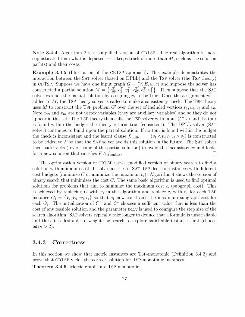
Note 3.4.4. Algorithm 2 is a simplified version of CBTSP. The real algorithm is moresophisticated than what is depicted — it keeps track of more than M , such as the solutionpath(s) and their costs.

Example 3.4.5 (Illustration of the CBTSP approach). This example demonstrates theinteraction between the SAT solver (based on DPLL) and the TSP solver (the TSP theory)in CBTSP. Suppose we have one input graph G = 〈V,E,w, c〉 and suppose the solver hasconstructed a partial solution M =

xT99, v

F2 , v

T1 , x

T67, v

T4 , v

T5

. Then suppose that the SAT

solver extends the partial solution by assigning v6 to be true. Once the assignment vT6 isadded to M , the TSP theory solver is called to make a consistency check. The TSP theoryuses M to construct the TSP problem G′ over the set of included vertices v1, v4, v5 and v6.Note x99 and x67 are not vertex variables (they are auxiliary variables) and so they do notappear in this set. The TSP theory then calls the TSP solver with input 〈G′, c〉 and if a touris found within the budget the theory returns true (consistent). The DPLL solver (SATsolver) continues to build upon the partial solution. If no tour is found within the budgetthe check is inconsistent and the learnt clause fconflict = ¬(v1 ∧ v4 ∧ v5 ∧ v6) is constructedto be added to F so that the SAT solver avoids this solution in the future. The SAT solverthen backtracks (revert some of the partial solution) to avoid the inconsistency and looksfor a new solution that satisfies F ∧ fconflict.

The optimization version of CBTSP uses a modified version of binary search to find asolution with minimum cost. It solves a series of SAT-TSP decision instances with differentcost budgets (minimize C or minimize the maximum ci). Algorithm 4 shows the version ofbinary search that minimizes the cost C. The same basic algorithm is used to find optimalsolutions for problems that aim to minimize the maximum cost ci (subgraph cost). Thisis achieved by replacing C with c1 in the algorithm and replace ci with c1 for each TSP

instance Gi = Vi, Ei, wi, ci so that c1 now constrains the maximum subgraph cost foreach Gi. The initialization of C+ and C∗ chooses a sufficient value that is less than thecost of any feasible solution and the parameter bdiv is used to configure the step size of thesearch algorithm. SAT solvers typically take longer to deduce that a formula is unsatisfiableand thus it is desirable to weight the search to explore satisfiable instances first (choosebdiv > 2).

3.4.3 Correctness

In this section we show that metric instances are TSP-monotonic (Definition 3.4.2) andprove that CBTSP yields the correct solution for TSP-monotonic instances.

Theorem 3.4.6. Metric graphs are TSP-monotonic.

27

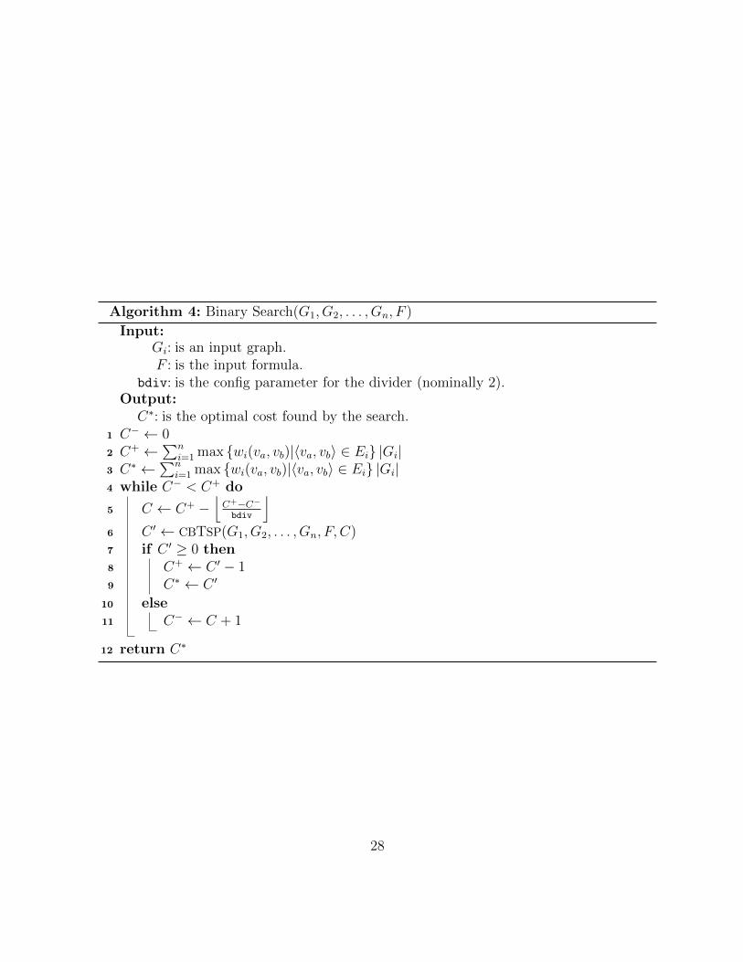
Algorithm 4: Binary Search(G1, G2, . . . , Gn, F )

Input:Gi: is an input graph.F : is the input formula.

bdiv: is the config parameter for the divider (nominally 2).Output:C∗: is the optimal cost found by the search.

1 C− ← 02 C+ ←

∑ni=1 max wi(va, vb)|〈va, vb〉 ∈ Ei |Gi|

3 C∗ ←∑n

i=1 max wi(va, vb)|〈va, vb〉 ∈ Ei |Gi|4 while C− < C+ do

5 C ← C+ −⌊C+−C−bdiv

⌋6 C ′ ← CBTSP(G1, G2, . . . , Gn, F, C)7 if C ′ ≥ 0 then8 C+ ← C ′ − 19 C∗ ← C ′

10 else11 C− ← C + 1

12 return C∗

28

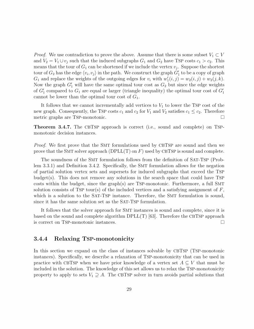
Proof. We use contradiction to prove the above. Assume that there is some subset V1 ⊂ Vand V2 = V1 ∪ vj such that the induced subgraphs G1 and G2 have TSP costs c1 > c2. Thismeans that the tour of G1 can be shortened if we include the vertex vj. Suppose the shortesttour of G2 has the edge 〈vi, vj〉 in the path. We construct the graph G′1 to be a copy of graphG1 and replace the weights of the outgoing edges for vi with w′1(i, j) = w2(i, j) + w2(j, k).Now the graph G′1 will have the same optimal tour cost as G2 but since the edge weightsof G′1 compared to G1 are equal or larger (triangle inequality) the optimal tour cost of G′1cannot be lower than the optimal tour cost of G1.

It follows that we cannot incrementally add vertices to V1 to lower the TSP cost of thenew graph. Consequently, the TSP costs c1 and c2 for V1 and V2 satisfies c1 ≤ c2. Thereforemetric graphs are TSP-monotonic.

Theorem 3.4.7. The CBTSP approach is correct (i.e., sound and complete) on TSP-monotonic decision instances.

Proof. We first prove that the SMT formulations used by CBTSP are sound and then weprove that the SMT solver approach (DPLL(T) on F ) used by CBTSP is sound and complete.

The soundness of the SMT formulation follows from the definition of SAT-TSP (Prob-lem 3.3.1) and Definition 3.4.2. Specifically, the SMT formulation allows for the negationof partial solution vertex sets and supersets for induced subgraphs that exceed the TSP

budget(s). This does not remove any solutions in the search space that could have TSP

costs within the budget, since the graph(s) are TSP-monotonic. Furthermore, a full SMT

solution consists of TSP tour(s) of the included vertices and a satisfying assignment of F ,which is a solution to the SAT-TSP instance. Therefore, the SMT formulation is sound,since it has the same solution set as the SAT-TSP formulation.

It follows that the solver approach for SMT instances is sound and complete, since it isbased on the sound and complete algorithm DPLL(T) [63]. Therefore the CBTSP approachis correct on TSP-monotonic instances.

3.4.4 Relaxing TSP-monotonicity

In this section we expand on the class of instances solvable by CBTSP (TSP-monotonicinstances). Specifically, we describe a relaxation of TSP-monotonicity that can be used inpractice with CBTSP when we have prior knowledge of a vertex set A ⊆ V that must beincluded in the solution. The knowledge of this set allows us to relax the TSP-monotonicityproperty to apply to sets V1 ⊇ A. The CBTSP solver in turn avoids partial solutions that

29

exclude vertices in the set A and thus the correctness of negating partial solutions is stillvalid.

To motivate this direction, let us consider the following example. Let G be a metricgraph with a start vertex vs and a goal vertex vg. Next, remove all the incoming edgesof vs and all the outgoing edges of vg other than the one edge connecting vg to vs. Also,modify the formula to be F = F ∧ vs ∧ vg. This example is not TSP-monotonic. However,the addition to the formula is so simple that the CBTSP solver’s preprocessing will assignvs and vg to be true (include vs and vg in the solution). Thus all partial solutions thatCBTSP checks will satisfy the TSP-monotonicity property, since the graph is otherwisemetric (preprocessing happens before any calls to the TSP theory).

The set of required vertices A, must not conflict with the formula F , i.e., F is satisfiableif and only if

F ∧

(∧v∈A

v

)is satisfiable. However, for this to work in practice, the decision to include the vertices inA would need to be done in the preprocessing step of CBTSP (before the DPLL solver iscalled, which is not discussed in this thesis). This happens for atomic clauses (clauses withonly one literal), e.g., a clause (v) would result in v being assigned true in the preprocessingphase of CBTSP.

Definition 3.4.8 (A-TSP-Monotonicity). Given a graph G = 〈V,E,w〉 and a subset A ⊂V , then G is A-TSP-monotonic if for any vertex subsets V1 ⊂ V2 ⊆ V such that A ⊆ V1,the induced subgraphs G1 and G2 have TSP costs c1 ≤ c2.

Proposition 3.4.9. The CBTSP approach is correct on A-TSP-monotonic decision in-stances if the decision to include the vertices in A are done so in the preprocessing phaseof the solver (before DPLL is called).

Proof. The proof follows Theorem’s 3.4.7 proof — the instance behaves like a TSP-monotonic instance once DPLL is called.

Remark 3.4.10 (TSP-monotonic examples). In addition to metric graphs being TSP-monotonic, disconnected metric subgraphs are also TSP-monotonic (each disconnectedcomponent of the graph is itself a complete metric subgraph).

We can connect metric subgraphs if we use the A-TSP-monotonicity relaxation. Anexample of an instance that satisfies the A-TSP-monotonicity is one where we have a set ofmetric (TSP-monotonic) subgraphs G1, G2, . . . , Gn that we would like the solution to visitsequentially as shown in Figure 3.2. Here we can see that if the black locations represent the

30

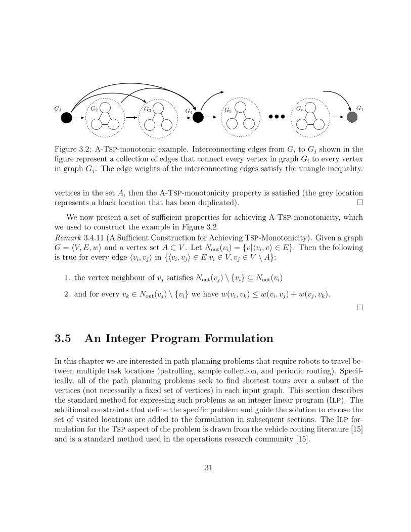
Figure 3.2: A-TSP-monotonic example. Interconnecting edges from Gi to Gj shown in thefigure represent a collection of edges that connect every vertex in graph Gi to every vertexin graph Gj. The edge weights of the interconnecting edges satisfy the triangle inequality.

vertices in the set A, then the A-TSP-monotonicity property is satisfied (the grey locationrepresents a black location that has been duplicated).

We now present a set of sufficient properties for achieving A-TSP-monotonicity, whichwe used to construct the example in Figure 3.2.

Remark 3.4.11 (A Sufficient Construction for Achieving TSP-Monotonicity). Given a graphG = 〈V,E,w〉 and a vertex set A ⊂ V . Let Nout(vi) = v|〈vi, v〉 ∈ E. Then the followingis true for every edge 〈vi, vj〉 in 〈vi, vj〉 ∈ E|vi ∈ V, vj ∈ V \ A:

1. the vertex neighbour of vj satisfies Nout(vj) \ vi ⊆ Nout(vi)

2. and for every vk ∈ Nout(vj) \ vi we have w(vi, vk) ≤ w(vi, vj) + w(vj, vk).

3.5 An Integer Program Formulation

In this chapter we are interested in path planning problems that require robots to travel be-tween multiple task locations (patrolling, sample collection, and periodic routing). Specif-ically, all of the path planning problems seek to find shortest tours over a subset of thevertices (not necessarily a fixed set of vertices) in each input graph. This section describesthe standard method for expressing such problems as an integer linear program (ILP). Theadditional constraints that define the specific problem and guide the solution to choose theset of visited locations are added to the formulation in subsequent sections. The ILP for-mulation for the TSP aspect of the problem is drawn from the vehicle routing literature [15]and is a standard method used in the operations research community [15].

31

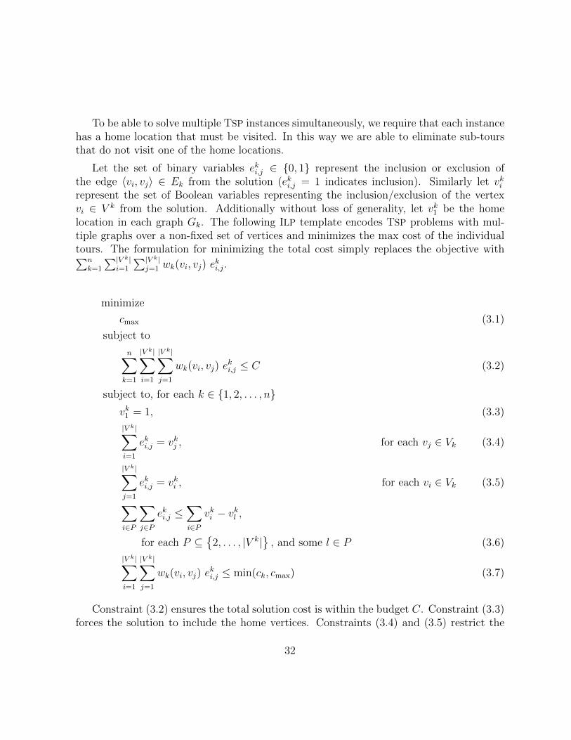
To be able to solve multiple TSP instances simultaneously, we require that each instancehas a home location that must be visited. In this way we are able to eliminate sub-toursthat do not visit one of the home locations.

Let the set of binary variables eki,j ∈ 0, 1 represent the inclusion or exclusion ofthe edge 〈vi, vj〉 ∈ Ek from the solution (eki,j = 1 indicates inclusion). Similarly let vkirepresent the set of Boolean variables representing the inclusion/exclusion of the vertexvi ∈ V k from the solution. Additionally without loss of generality, let vk1 be the homelocation in each graph Gk. The following ILP template encodes TSP problems with mul-tiple graphs over a non-fixed set of vertices and minimizes the max cost of the individualtours. The formulation for minimizing the total cost simply replaces the objective with∑n

k=1

∑|V k|i=1

∑|V k|j=1 wk(vi, vj) e

ki,j.

minimize

cmax (3.1)

subject to

n∑k=1

|V k|∑i=1

|V k|∑j=1

wk(vi, vj) eki,j ≤ C (3.2)

subject to, for each k ∈ 1, 2, . . . , nvk1 = 1, (3.3)

|V k|∑i=1

eki,j = vkj , for each vj ∈ Vk (3.4)

|V k|∑j=1

eki,j = vki , for each vi ∈ Vk (3.5)∑i∈P

∑j∈P

eki,j ≤∑i∈P

vki − vkl ,

for each P ⊆

2, . . . , |V k|

, and some l ∈ P (3.6)

|V k|∑i=1

|V k|∑j=1

wk(vi, vj) eki,j ≤ min(ck, cmax) (3.7)

Constraint (3.2) ensures the total solution cost is within the budget C. Constraint (3.3)forces the solution to include the home vertices. Constraints (3.4) and (3.5) restrict the

32

incoming and outgoing degree for each location to be one only if the vertex is included.Constraint (3.6) is the sub-tour elimination constraint, where a sub-tour that visits theset P but not location 1 is eliminated by ensuring that the number of edges betweenvertices in P cannot equal |P | (if each vertex in P is visited then

∑i∈P v

ki − vkl = |P | − 1).

Otherwise if location l is not visited then the inequality is satisfied by the other constraints(each included vertex has at most one incoming and one outgoing edge). In practice thesub-tour elimination constraint is lazily implemented (if a constraint in (3.6) is violatedduring the construction of the solution, then the constraint is added to the formulation) toavoid expressing an exponential number of constraints. Finally, Constraint (3.7) ensuresthe individual tours are within the budgets ck and it ensures that the individual tour costsare equal or lower than the optimal value cmax.

3.6 Robotic Applications and Expressions

In this section we describe three robotic path planning problems (patrolling, sample col-lection, and periodic routing) and show how they are expressed in both SAT-TSP and ILP.The SAT-TSP expressions for these problems utilize at-most-one-in-a-set constraints. Wedefine this type of constraint here and use it throughout the rest of the section.

Definition 3.6.1 (At-most-one-in-a-set constraint). Given a set X ′ ⊂ X of variables,the at-most-one-in-a-set constraint states that at most one variable in the set X ′ can beassigned true. The following Boolean formula expresses the constraint:∨

x,y∈X′|x 6=y

¬(x ∧ y).

Remark 3.6.2 (Expressions). The expressions presented in this section are the expressionsthat we have found perform the best. As with the MTZ ILP expression for TSP [57], onecan learn later that better expressions exist.

3.6.1 The Patrolling Problem

We consider patrolling problems that require each point of interest to be observed frommultiple viewpoints. These problems were inspired by patrolling problems that allow thepoints of interest to be observed from multiple viewpoints [65, 7]. Our patrolling problemis defined on a metric environment that contains m points of interest, n− 1 “observation

33

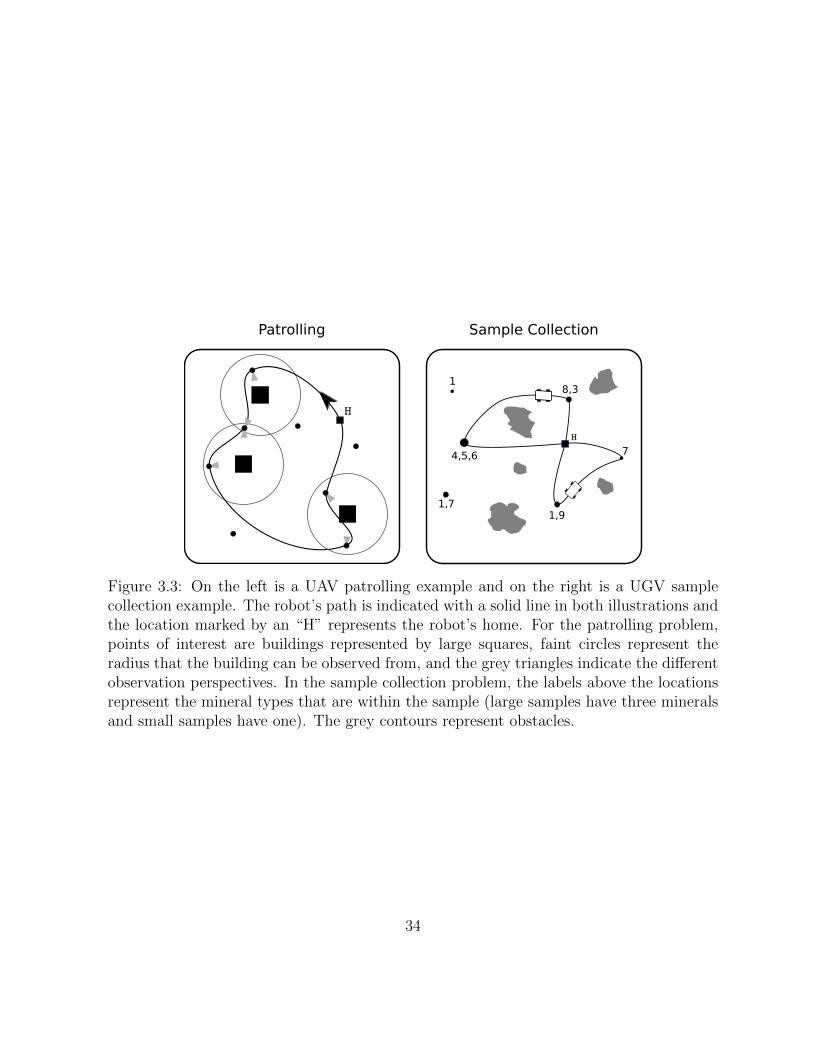
4,5,6

18,3

7

1,91,7

H

Patrolling Sample Collection

H

Figure 3.3: On the left is a UAV patrolling example and on the right is a UGV samplecollection example. The robot’s path is indicated with a solid line in both illustrations andthe location marked by an “H” represents the robot’s home. For the patrolling problem,points of interest are buildings represented by large squares, faint circles represent theradius that the building can be observed from, and the grey triangles indicate the differentobservation perspectives. In the sample collection problem, the labels above the locationsrepresent the mineral types that are within the sample (large samples have three mineralsand small samples have one). The grey contours represent obstacles.

34

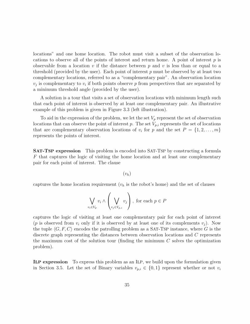
locations” and one home location. The robot must visit a subset of the observation lo-cations to observe all of the points of interest and return home. A point of interest p isobservable from a location v if the distance between p and v is less than or equal to athreshold (provided by the user). Each point of interest p must be observed by at least twocomplementary locations, referred to as a “complementary pair”. An observation locationvj is complementary to vi if both points observe p from perspectives that are separated bya minimum threshold angle (provided by the user).

A solution is a tour that visits a set of observation locations with minimum length suchthat each point of interest is observed by at least one complementary pair. An illustrativeexample of this problem is given in Figure 3.3 (left illustration).

To aid in the expression of the problem, we let the set Vp represent the set of observationlocations that can observe the point of interest p. The set Vp,i represents the set of locationsthat are complementary observation locations of vi for p and the set P = 1, 2, . . . ,mrepresents the points of interest.

SAT-TSP expression This problem is encoded into SAT-TSP by constructing a formulaF that captures the logic of visiting the home location and at least one complementarypair for each point of interest. The clause

(vh)

captures the home location requirement (vh is the robot’s home) and the set of clauses

∨vi∈Vp

vi ∧

∨vj∈Vp,i

vj

, for each p ∈ P

captures the logic of visiting at least one complementary pair for each point of interest(p is observed from vi only if it is observed by at least one of its complements vj). Nowthe tuple 〈G,F,C〉 encodes the patrolling problem as a SAT-TSP instance, where G is thediscrete graph representing the distances between observation locations and C representsthe maximum cost of the solution tour (finding the minimum C solves the optimizationproblem).

ILP expression To express this problem as an ILP, we build upon the formulation givenin Section 3.5. Let the set of Binary variables vp,i ∈ 0, 1 represent whether or not vi

35

is part of a complementary pair observing the point of interest p. The following are theadditional constraints in the ILP formulation.

for each p ∈ 1, 2, . . . ,mvp,i ≤ vi, for each vi ∈ Vp (3.8)

vp,i ≤∑vj∈Vp,i

vj, for each vi ∈ Vp (3.9)

∑vi∈Vp

vp,i ≥ 1 (3.10)

Constraint (3.8) restricts the indicator vp,i from being true if the location vi itself isnot visited, Constraint (3.9) restricts the indicator from being true if none of the com-plementary locations of vi are visited, and Constraint (3.10) ensures that at least onecomplementary pair is visited.

3.6.2 The Sample Collection Problem

The following problem is inspired by sample collection problems that arise for sciencerovers [26]. In this problem, we have a set of R robots, n− 1 samples, one home location,and a set of m different minerals that can appear in the n−1 samples. Each sample in theenvironment is either small, medium, or large. Small samples have within them one typeof mineral, medium samples have up to two different minerals, and large samples have upto three different minerals. There are two types of robots used to collect samples, smalland large. A small robot can collect an unlimited number of small samples and up to onemedium sample but no large samples. A large robot cannot collect small samples, but itcan collect an unlimited number of medium samples and up to one large sample. The smalland large robots may have different speeds. Each robot is given the same time budget tocollect samples and return home. Since each location only contains one sample, multiplerobots are restricted from visiting the same location.

A solution to this problem is a tour for each robot that satisfies the time budget, startsat the home location, and visits a set of locations in the environment that allows therobots to collect a set of samples that contain one of each type of mineral found in theenvironment. An optimal solution minimizes the total time taken by the set of robots. Anillustrative example of this problem is given in Figure 3.3 (on the right). In this example

36

there are no samples with mineral 2 and so feasible solutions do not collect mineral 2.Additionally, we demonstrate a sample collection solution in a demo video1. This solutionutilizes one small and one large robot to collect seven different mineral types.

To express this problem we introduce the following. Let Vt be the set of locations thatcontains a mineral of type t; let VS, VM and VL be the set of locations that respectivelyhave small, medium and large samples; let RS, RL and R = 1, 2, . . . , |R| respectively bethe set of small, large, and all robots; and let T = 1, 2, . . . ,m be the set of minerals.

SAT-TSP expression The problem is encoded as a SAT-TSP instance by constructing agraph Gr for each robot r and a formula F that captures the goals and capacity restrictionsof the robots. Each graph Gr contains all of the locations in the environment and its edgeweights are given by transitions for robot r to move within its environment. The set ofvariables vi,r is used to indicate if robot r visits location i. When the location/robot pair isincompatible, such as location i contains a large sample and robot r is small, the variableis negated. We chose this approach instead of constructing graphs without incompatiblelocation/robot pairs to simplify the SAT-TSP expression in this chapter.

We start our expression by forcing each robot to visit the home location using theclauses ∧

r∈R

vh,r,

where vh ∈ V is the home location for the robots. Next, we negate all incompatiblelocation/robot pairs (e.g., small robot large sample)∧

vi,r∈XI

¬vi,r,

whereXI = vi,r|vi ∈ VL, r ∈ RS ∪ vi,r|vi ∈ VS, r ∈ RL .

We encode the goal of collecting at least one of each mineral (if the mineral exists), witha disjunctive clause for each mineral

∧t∈T

( ∨vi∈Vt,r∈R

vi,r

).


37


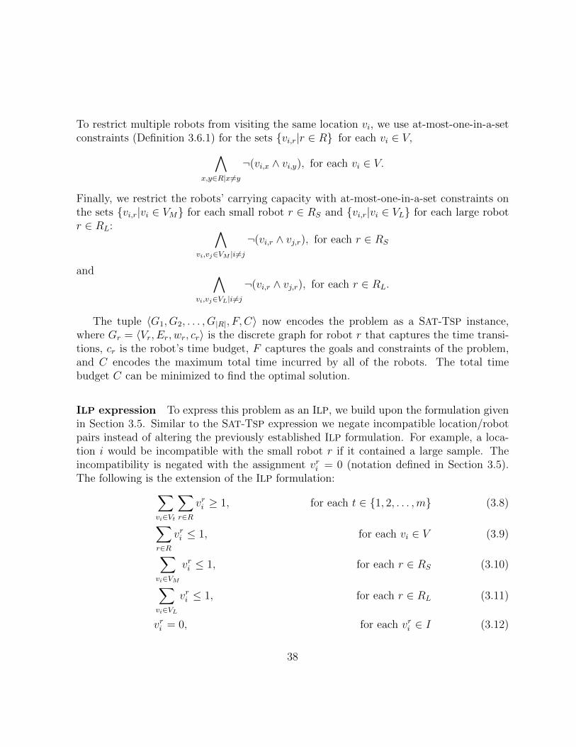
To restrict multiple robots from visiting the same location vi, we use at-most-one-in-a-setconstraints (Definition 3.6.1) for the sets vi,r|r ∈ R for each vi ∈ V,∧

x,y∈R|x 6=y

¬(vi,x ∧ vi,y), for each vi ∈ V.

Finally, we restrict the robots’ carrying capacity with at-most-one-in-a-set constraints onthe sets vi,r|vi ∈ VM for each small robot r ∈ RS and vi,r|vi ∈ VL for each large robotr ∈ RL: ∧

vi,vj∈VM |i 6=j

¬(vi,r ∧ vj,r), for each r ∈ RS

and ∧vi,vj∈VL|i 6=j

¬(vi,r ∧ vj,r), for each r ∈ RL.

The tuple 〈G1, G2, . . . , G|R|, F, C〉 now encodes the problem as a SAT-TSP instance,where Gr = 〈Vr, Er, wr, cr〉 is the discrete graph for robot r that captures the time transi-tions, cr is the robot’s time budget, F captures the goals and constraints of the problem,and C encodes the maximum total time incurred by all of the robots. The total timebudget C can be minimized to find the optimal solution.

ILP expression To express this problem as an ILP, we build upon the formulation givenin Section 3.5. Similar to the SAT-TSP expression we negate incompatible location/robotpairs instead of altering the previously established ILP formulation. For example, a loca-tion i would be incompatible with the small robot r if it contained a large sample. Theincompatibility is negated with the assignment vri = 0 (notation defined in Section 3.5).The following is the extension of the ILP formulation:∑

vi∈Vt

∑r∈R

vri ≥ 1, for each t ∈ 1, 2, . . . ,m (3.8)∑r∈R

vri ≤ 1, for each vi ∈ V (3.9)∑vi∈VM

vri ≤ 1, for each r ∈ RS (3.10)∑vi∈VL

vri ≤ 1, for each r ∈ RL (3.11)

vri = 0, for each vri ∈ I (3.12)

38

where I = vri |vi ∈ VL, r ∈ Rs∪vri |vi ∈ VS, r ∈ RL is used to represent the set of incom-patible location/robot pairs. Constraint (3.8) encodes the goal of retrieving at least one ofeach mineral type (if it exists), Constraint (3.9) restricts multiple robots from retrievingthe same sample, Constraint (3.10) restricts small robots from collecting more than onemedium sample, Constraint (3.11) restricts small robots from collecting more than onelarge sample, and Constraint (3.12) negates the incompatible location/robot pairs.

3.6.3 The Period Routing Problem

The period routing problem [11, 100] requires a robot (vehicle) to service a set of n − 1locations over a set of m periods. In each period the robot starts from a designated homelocation and travels to a subset of the service locations. Each location v requires f(v) ≤ mout of m periods of service and has restrictions on which periods or period combinations areallowed. For this chapter, locations restrict back to back service (the first and last periodare also considered back to back). This problem arises in collection [100] and delivery [11]tasks. Also period routing problems often contain a capacity that limits the number oftasks that can be performed.

A solution to this problem is a set of tours, one for each period that meets the servicedemands of the locations, respects the capacity limits, and respects the service restrictions.The optimal solution minimizes the maximum length tour over the m periods.

SAT-TSP expression The problem is encoded as a SAT-TSP instance by constructing agraph for each period and a formula that captures the goals and restrictions of the problem.Each graph Gp represents the transition costs for the robot to move within its environmentduring period p (all graphs are the same).

The problem goals of providing a specific number of service periods to the locationsis captured with the standard technique of using adder circuits [55], which are efficientlytranslated to a Boolean formula [41] and added to F . These adder circuits take as input theset of location/period variables for each location vi,p|p ∈ P and output a set of Booleanvariables bi,1, bi,2, bi,4, . . . that capture the binary encoding of how many of the inputsare true. Following that, the outputs of the adder circuit are forced to the desired servicedemands, f(vi). As an example, if vi requires two visits, then we force the twos bit, bi,2, tobe true and the remaining bits to be false. This is accomplished by adding the followingto F ← F ∧ ¬bi,1 ∧ bi,2 ∧ ¬bi,4 ∧ . . ..

39

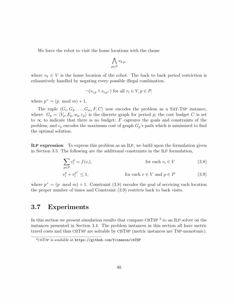
We force the robot to visit the home locations with the clause∧p∈P

vh,p,

where vh ∈ V is the home location of the robot. The back to back period restriction isexhaustively handled by negating every possible illegal combination.

¬(vi,p ∧ vi,p+) for all vi ∈ V, p ∈ P,

where p+ = (p mod m) + 1.

The tuple 〈G1, G2, . . . , Gm, F, C〉 now encodes the problem as a SAT-TSP instance,where: Gp = 〈Vp, Ep, wp, cp〉 is the discrete graph for period p; the cost budget C is setto ∞ to indicate that there is no budget; F captures the goals and constraints of theproblem; and cp encodes the maximum cost of graph Gp’s path which is minimized to findthe optimal solution.

ILP expression To express this problem as an ILP, we build upon the formulation givenin Section 3.5. The following are the additional constraints in the ILP formulation,∑

p∈P

vpi = f(vi), for each vi ∈ V (3.8)

vpi + vp+

i ≤ 1, for each v ∈ V and p ∈ P (3.9)

where p+ = (p mod m) + 1. Constraint (3.8) encodes the goal of servicing each locationthe proper number of times and Constraint (3.9) restricts back to back visits.

3.7 Experiments

In this section we present simulation results that compare CBTSP 2 to an ILP solver on theinstances presented in Section 3.4. The problem instances in this section all have metrictravel costs and thus CBTSP are solvable by CBTSP (metric instances are TSP-monotonic).

2CBTSP is available at https://github.com/fcimeson/cbTSP

40

https://github.com/fcimeson/cbTSP

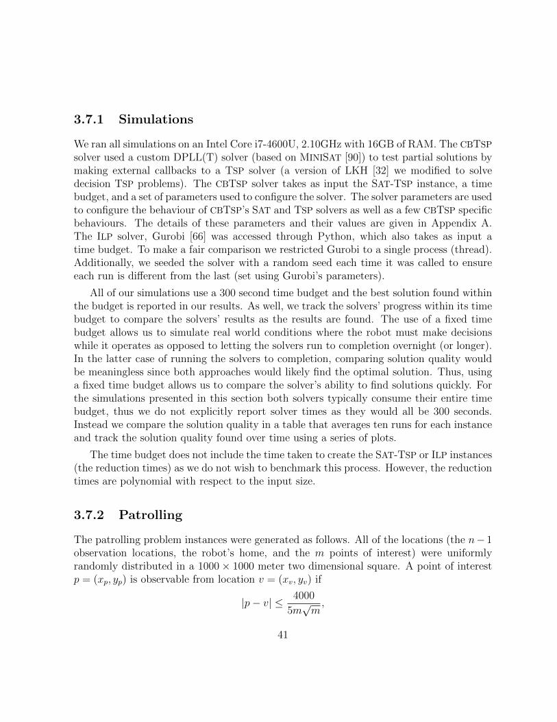
3.7.1 Simulations

We ran all simulations on an Intel Core i7-4600U, 2.10GHz with 16GB of RAM. The CBTSP

solver used a custom DPLL(T) solver (based on MINISAT [90]) to test partial solutions bymaking external callbacks to a TSP solver (a version of LKH [32] we modified to solvedecision TSP problems). The CBTSP solver takes as input the SAT-TSP instance, a timebudget, and a set of parameters used to configure the solver. The solver parameters are usedto configure the behaviour of CBTSP’s SAT and TSP solvers as well as a few CBTSP specificbehaviours. The details of these parameters and their values are given in Appendix A.The ILP solver, Gurobi [66] was accessed through Python, which also takes as input atime budget. To make a fair comparison we restricted Gurobi to a single process (thread).Additionally, we seeded the solver with a random seed each time it was called to ensureeach run is different from the last (set using Gurobi’s parameters).

All of our simulations use a 300 second time budget and the best solution found withinthe budget is reported in our results. As well, we track the solvers’ progress within its timebudget to compare the solvers’ results as the results are found. The use of a fixed timebudget allows us to simulate real world conditions where the robot must make decisionswhile it operates as opposed to letting the solvers run to completion overnight (or longer).In the latter case of running the solvers to completion, comparing solution quality wouldbe meaningless since both approaches would likely find the optimal solution. Thus, usinga fixed time budget allows us to compare the solver’s ability to find solutions quickly. Forthe simulations presented in this section both solvers typically consume their entire timebudget, thus we do not explicitly report solver times as they would all be 300 seconds.Instead we compare the solution quality in a table that averages ten runs for each instanceand track the solution quality found over time using a series of plots.

The time budget does not include the time taken to create the SAT-TSP or ILP instances(the reduction times) as we do not wish to benchmark this process. However, the reductiontimes are polynomial with respect to the input size.

3.7.2 Patrolling

The patrolling problem instances were generated as follows. All of the locations (the n− 1observation locations, the robot’s home, and the m points of interest) were uniformlyrandomly distributed in a 1000× 1000 meter two dimensional square. A point of interestp = (xp, yp) is observable from location v = (xv, yv) if

|p− v| ≤ 4000

5m√m,

41

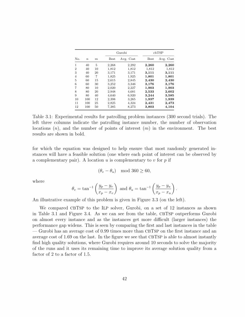
Gurobi cbTSP

No. n m Best Avg. Cost Best Avg. Cost

1 40 5 2,268 2,292 2,260 2,2602 40 10 1,812 1,812 1,812 1,8123 40 20 3,171 3,171 3,111 3,1114 60 7 1,825 1,925 1,801 1,8015 60 15 2,615 2,845 2,430 2,4306 60 30 3,252 3,346 3,176 3,1767 80 10 2,020 2,227 1,903 1,9038 80 20 2,948 4,681 2,533 2,6029 80 40 4,640 6,920 3,244 3,58510 100 12 2,398 3,265 1,937 1,93911 100 25 2,825 4,324 2,431 2,47312 100 50 7,385 8,273 3,803 4,104

Table 3.1: Experimental results for patrolling problem instances (300 second trials). Theleft three columns indicate the patrolling instance number, the number of observationlocations (n), and the number of points of interest (m) in the environment. The bestresults are shown in bold.

for which the equation was designed to help ensure that most randomly generated in-stances will have a feasible solution (one where each point of interest can be observed bya complementary pair). A location u is complementary to v for p if

(θv − θu) mod 360 ≥ 60,

where

θv = tan−1

(yp − yvxp − xv

)and θu = tan−1

(yp − yuxp − xu

).

An illustrative example of this problem is given in Figure 3.3 (on the left).

We compared CBTSP to the ILP solver, Gurobi, on a set of 12 instances as shownin Table 3.1 and Figure 3.4. As we can see from the table, CBTSP outperforms Gurobion almost every instance and as the instances get more difficult (larger instances) theperformance gap widens. This is seen by comparing the first and last instances in the table— Gurobi has an average cost of 0.99 times more than CBTSP on the first instance and anaverage cost of 1.69 on the last. In the figure we see that CBTSP is able to almost instantlyfind high quality solutions, where Gurobi requires around 10 seconds to solve the majorityof the runs and it uses its remaining time to improve its average solution quality from afactor of 2 to a factor of 1.5.

42

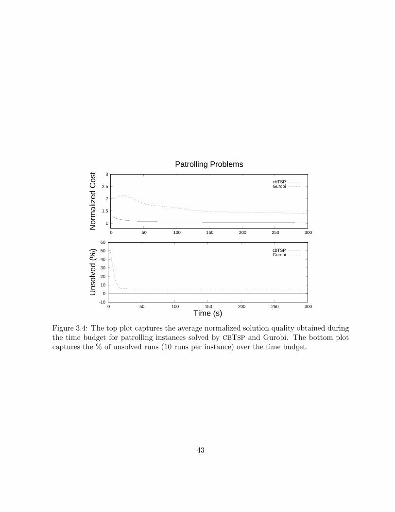
1

1.5

2

2.5

3

0 50 100 150 200 250 300

Nor

mal

ized

Cos

t

Patrolling Problems

cbTSPGurobi

-10

0

10

20

30

40

50

60

0 50 100 150 200 250 300

Uns

olve

d (%

)

Time (s)

cbTSPGurobi

Figure 3.4: The top plot captures the average normalized solution quality obtained duringthe time budget for patrolling instances solved by CBTSP and Gurobi. The bottom plotcaptures the % of unsolved runs (10 runs per instance) over the time budget.

43

3.7.3 Sample Collection

The sample collection problem instances we tested were generated as follows. There isone home location and n − 1 sample locations in the environment and the set of samplescontain up to m different mineral types. All locations (sample locations and the homelocation) were uniformly randomly distributed in a 1000 × 1000 meter two dimensionalsquare. The distribution of sample sizes are as follows: 3:1 for small to large and 2:1 forsmall to medium. The types of minerals in each sample are uniformly randomly distributed(the same mineral type may reoccur in a sample). There are two types of robots used tocollect samples, small and large, three of each, six in total. Each robot has a time budgetof 25 minutes to collect samples and return home and the small robots travel at a speedof 2m/s, while the large robots travel at half that speed (1m/s).

Note 3.7.1. Although the large robots can complete the task by collecting about half thesamples, it costs double to travel the same distance. Furthermore, it is equally likely for amineral type to be found in a small, medium, or large sample.

We compared CBTSP to the ILP solver, Gurobi, on 12 sample collection instances andreported the data in Table 3.2 and Figure 3.5. The results show that CBTSP is compet-itive with Gurobi. Specifically, both solvers find the same quality solutions for the easyinstances (instances 1-3 in the table — the smaller instances); then as the instances moveinto the medium difficult range (instances 4-7), CBTSP starts to outperform Gurobi; andonce the instances become difficult (instances 8-12 — the largest instances) CBTSP oftenoutperforms Gurobi by quite a bit. Here, Gurobi only outperforms CBTSP on one instanceand fails to find feasible solutions for two out of five difficult instances. From Figure 3.5,we see that CBTSP is able to solve each run within the first 20 seconds, while Gurobi isnot able to find feasible solutions for more than 20% of the runs. Additionally, we see thatat first CBTSP finds some pretty low quality solutions (2-4.5 times the best known) and ittakes CBTSP about 100 seconds to improve this quality to within 1.5 of the best known.Although, not shown here, the runs that take longer to improve are the larger/more diffi-cult instances, some of which do not show up in Gurobi’s average because Gurobi was notable to find feasible solutions. Thus, CBTSP is able to solve more instances and find higherquality solutions than Gurobi.

Physical simulations We have also performed simulation experiments for sample col-lection in more complex environments where travel costs are shortest collision free paths.These simulations utilize the Clearpath Husky robot model within Gazebo. The robotsuse the ROS navigation stack [75] to move within the physical simulator. An example

44

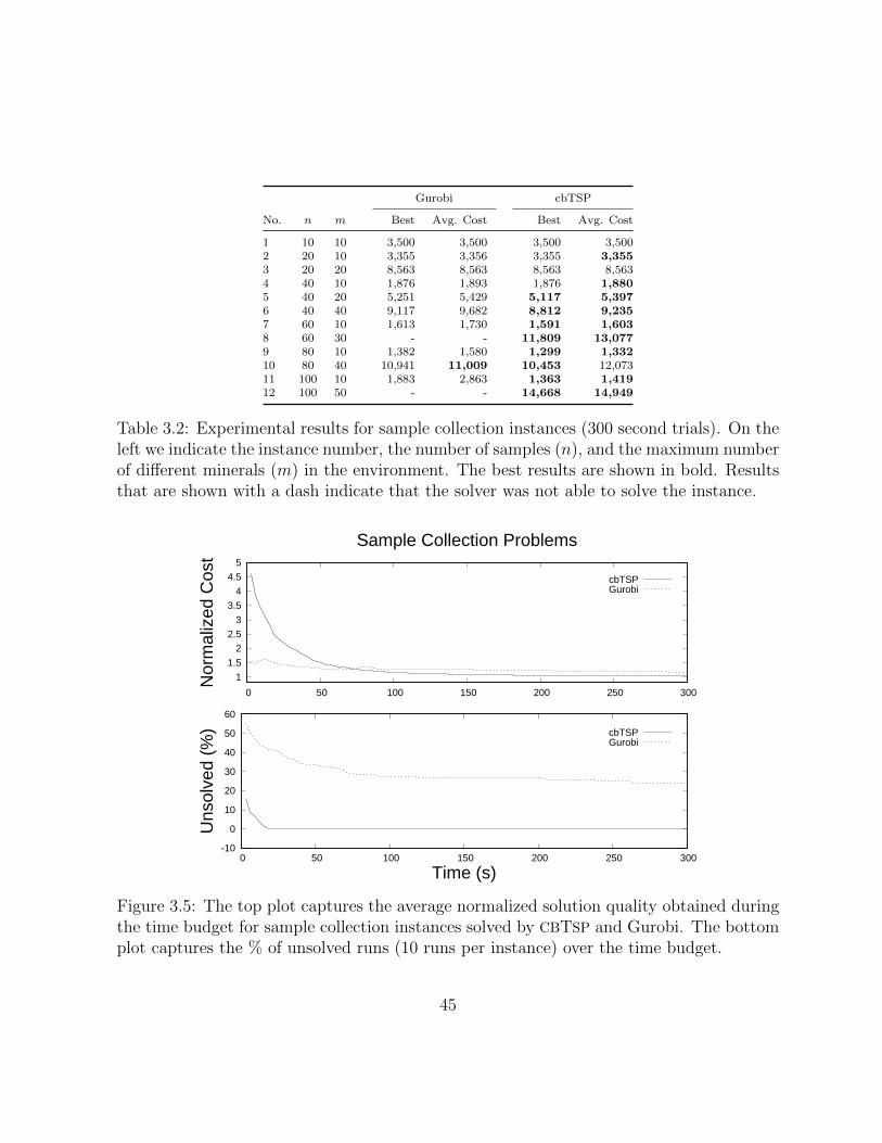
Gurobi cbTSP

No. n m Best Avg. Cost Best Avg. Cost

1 10 10 3,500 3,500 3,500 3,5002 20 10 3,355 3,356 3,355 3,3553 20 20 8,563 8,563 8,563 8,5634 40 10 1,876 1,893 1,876 1,8805 40 20 5,251 5,429 5,117 5,3976 40 40 9,117 9,682 8,812 9,2357 60 10 1,613 1,730 1,591 1,6038 60 30 - - 11,809 13,0779 80 10 1,382 1,580 1,299 1,33210 80 40 10,941 11,009 10,453 12,07311 100 10 1,883 2,863 1,363 1,41912 100 50 - - 14,668 14,949

Table 3.2: Experimental results for sample collection instances (300 second trials). On theleft we indicate the instance number, the number of samples (n), and the maximum numberof different minerals (m) in the environment. The best results are shown in bold. Resultsthat are shown with a dash indicate that the solver was not able to solve the instance.

1

1.5

2

2.5

3

3.5

4

4.5

5

0 50 100 150 200 250 300

Nor

mal

ized

Cos

t

Sample Collection Problems

cbTSPGurobi

-10

0

10

20

30

40

50

60

0 50 100 150 200 250 300

Uns

olve

d (%

)

Time (s)

cbTSPGurobi

Figure 3.5: The top plot captures the average normalized solution quality obtained duringthe time budget for sample collection instances solved by CBTSP and Gurobi. The bottomplot captures the % of unsolved runs (10 runs per instance) over the time budget.

45

H2 2

1

1 1

1 1 1

1 1 1

H2 2

1

1 1

1 1 1

1 1 1

Period 1 Period 2

1 1

Figure 3.6: A simple period routing example for material transport within a factory. Thereare only two periods of service and a location can either require service for one or bothperiods (as indicated on the graph). The home location is labelled with an “H”.

simulation, visualized with RViz is shown in Figure 1.1 and demoed in our video3. In thevideo there are two robots, each with different speed. The slower Husky emulates the largesample collecting robot and the faster Husky emulates the small robot. The collection taskrequires collecting seven different mineral types from the environment.

3.7.4 Period Routing

The period routing problem instances were generated as follows. All of the locations (then − 1 service locations and the robot’s home) were uniformly randomly distributed in a1000 × 1000 meter two dimensional square. There are six service periods; each servicelocation may require either one, two, or three periods of service (uniformly randomlyassigned) out of the six periods. An illustrative example is shown in Figure 3.6.

We have compared CBTSP to the ILP solver Gurobi, on 12 period routing instances, forwhich the results can be found in Table 3.3 and Figure 3.7. The table shows that CBTSP

outperforms Gurobi on all of the instances and like the other two applications, as theinstances become more difficult the performance gap between CBTSP and Gurobi grows.This can be seen as a trend between the first and last instance in the table. Gurobi is on


46


Gurobi cbTSP

No. n Best Avg. Cost Best Avg. Cost

1 15 2,278 2,392 2,212 2,2122 15 1,968 2,055 1,904 1,9043 20 2,200 2,382 2,022 2,0224 20 1,807 2,016 1,670 1,6705 25 2,706 3,718 2,310 2,3476 25 2,638 2,869 2,057 2,0577 30 2,877 3,133 2,342 2,3588 30 3,040 3,811 2,433 2,4399 35 3,738 3,944 2,502 2,61010 35 3,667 3,902 2,404 2,50611 40 4,369 4,680 2,727 2,95412 40 3,934 4,529 2,594 2,678

Table 3.3: Experimental results for period routing problem instances (300 second trials).The left two columns indicate the instance number and the number of locations in theenvironment. The best results are shown in bold.

par with CBTSP for the first instance and then for the last instance Gurobi has a solutionquality that is 3.66 times worse than CBTSP’s. From the figure, we see that CBTSP isable to find feasible solutions for all of the runs within the first 10 seconds, while in thesame time frame Gurobi was only able to find feasible solutions for approximately 70% ofthe runs. Additionally, Gurobi struggled finding high quality solutions for these problems,while CBTSP was able to find reasonably good quality solutions within the first 60 seconds.

3.8 Summary

In summary, this chapter provided an alternative approach for solving high-level path plan-ning problems, called SAT-TSP. We used the SAT-TSP problem as the modelling languagefor expressing high-level path planning problems. We provided the SAT-TSP solver CBTSP

for finding path planning solutions and proved its correctness for TSP-monotonic instances.Additionally, we provided a relaxation of TSP-monotonicity that expanded the set of solv-able problems by CBTSP. Through a series of experiments we demonstrated that CBTSP

often outperforms a commercial grade ILP solver — especially on difficult instances. Thusshowing that CBTSP is a strong candidate for solving discrete path planning problems.The CBTSP solver can be downloaded from https://github.com/fcimeson/cbTSP.

47


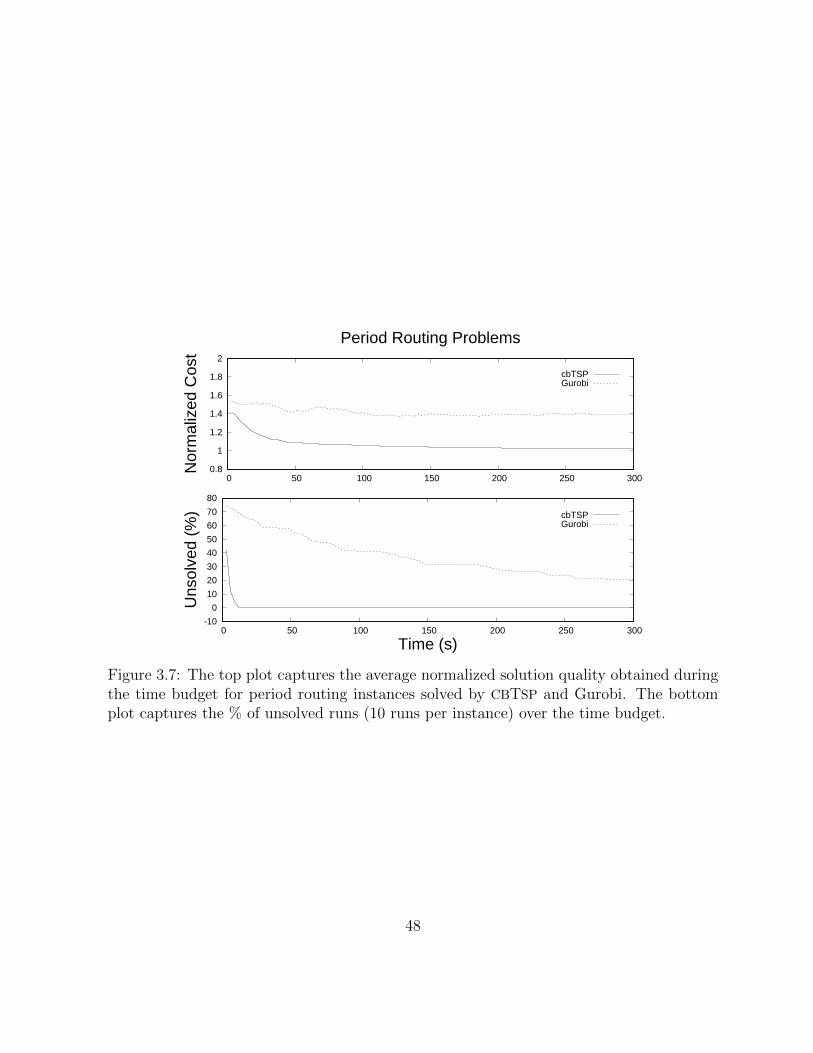
0.8

1

1.2

1.4

1.6

1.8

2

0 50 100 150 200 250 300

Nor

mal

ized

Cos

t

Period Routing Problems

cbTSPGurobi

-10

0

10

20

30

40

50

60

70

80

0 50 100 150 200 250 300

Uns

olve

d (%

)

Time (s)

cbTSPGurobi

Figure 3.7: The top plot captures the average normalized solution quality obtained duringthe time budget for period routing instances solved by CBTSP and Gurobi. The bottomplot captures the % of unsolved runs (10 runs per instance) over the time budget.

48

Chapter 4

Pruning Solutions

This chapter introduces two approaches for pruning path planning solutions from the searchspace. These approaches are used in conjunction with existing path planning solvers toimprove the solver’s efficiency. The boost in efficiency comes at the expense of solutionquality. However, we show in this chapter that solutions found using these approaches arewithin a constant factor of the optimal. We focus on the class of discrete path planningproblems that do not contain ordering constraints.

The first approach, coupled planning, starts by partitioning the environment into a setof clusters/regions. Then it creates a new version of the problem, the clustered version,to restrict how feasible paths visit the set of clusters. This restriction prunes a significantportion of the solution search space.

The second approach, hierarchical planning, is an extension of the first approach thatfurther prunes the solution search. This approach uses the clusters to decompose theproblem into a hierarchy of small independent problems, where each problem representsa coarse approximation of the environment or sub-region. The solver starts by building apath on the coarsest level and then extends its solution to the next level by visiting thenested components of its coarsened path. This process repeats until a solution is found forthe full problem.

These approaches achieve their solution quality guarantees (bounds) from how theypartition the environment. Specifically, these approaches use a new clustering/partition-ing method called Γ-Clustering that we developed specifically for path planning. A Γ-Clustering is a collection of clusters that have their locations close to each other and farfrom all other locations. See Figure 4.1 for a sample Γ-Clustering of an office environment(the 5th floor of the E5 building at the University of Waterloo). The parameter Γ is used

49

to specify the degree of separation that each Γ-Cluster must achieve (distance from otherlocations). Unlike other clustering methods, the Γ-Clustering method does not take in asinput, an integer k for finding the best k set of clusters. Instead it takes in as input theparameter Γ and finds the Γ-Clusters within the environment that achieve the standardsimposed by the Γ parameter. Thus some problems contain many Γ-Clusters while otherscontain little to none.

The contributions of this chapter are as follows. We introduce a new clustering method,Γ-Clustering, that is specifically designed for discrete path planning. We provide an efficientalgorithm based on minimum spanning trees (MST) for computing the optimal clusteringand prove that this clustering is unique. We introduce the coupled planning approach asa method for pruning the search space and prove that solutions found using this approachare within a constant factor of min(2, 1 + 3

2Γ) of the optimal. We then introduce hierarchi-

cal planning with Γ-Clusterings and prove that solutions found by this method are withina constant factor of min(2 + 4

Γ, 1 + 13

2Γ) of the optimal. Our benchmark compares these

two approaches to a standard non-clustered approach, where we use an ILP solver witha time budget of 900 seconds to find path planning solutions. The results show that thepath quality obtained by these two methods are much closer to the optimal cost than theconstant factor bounds. Most solutions obtained from our approaches were within 10% ofthe optimal, where the coupled approach was able to outperform the hierarchical approachon the easy instances. For the instances that finished within the allotted time budget, thecoupled and hierarchical approaches showed a substantial time savings compared to thenon-clustered approach. For the instances that consumed the time budget, the clusteredapproaches were able to maintain their performance longer than the non-clustered ap-proach, where the hierarchical approach was able to maintain its performance longer thanthe coupled approach. Additionally, our benchmark compares the quality of Γ-Clusteringsto clusterings found with five different methods. The results for these comparisons showthat when planning with clusters, Γ-Clusterings produce higher quality solutions than othertypes of clusterings methods.

The rest of this chapter is organized as follows. Section 4.1 reviews the related work forthese approaches. Section 4.2 provides the background needed for this chapter. Section 4.3defines the set of path planning problems considered by this chapter. Section 4.4 formallydefines what Γ-Clusters are and how to find them. Section 4.5 defines the coupled planningapproach, then Section 4.6 introduces decoupled planning as a lead-in to hierarchical plan-ning presented in Section 4.7. The benchmark is presented and discussed in Section 4.8.The chapter summary is given in Section 4.9.

50

Figure 4.1: The results of Γ-Clustering used on an office environment. The red trianglesrepresent locations of interest and the red boxes surround clusters of size two or greater.

4.1 Related Work

This section builds upon Section 1.1 to provide a more in depth review of the literaturerelated to this chapter.

There are a number of pruning techniques for reducing the search space, such as branchand bound [51, 13]. Like our approach, these approaches can sometimes be used in tandemwith each other to prune larger regions of the search space. In fact, the hierarchical planningapproach presented in this chapter is a combination of the coupled planning approach witha hierarchical approach.

The general form of hierarchical planning decomposes the environment into regions andplans those regions as approximations instead of planning on the full resolution problem.This practice has been done under the guise of hierarchical highways [82], cell decomposi-tion [104, 9], hierarchical planning with maps [105], and multi-resolution planning [43, 53].Most of these approaches are used for point-to-point planning. However, there is a bodyof work that addresses solving vehicle routing problems, such as TSP for Euclidean envi-ronments [22, 31, 58, 5]. Our approach goes beyond Euclidean environments and the TSP,as it handles metric environments and works for a class of vehicle routing problems that

51

encompasses TSP.

Multilevel refinement is a framework similar to hierarchical planning and has beenused to solve vehicle routing problems. At its most basic level, the framework recursivelycoarsens a problem into a hierarchy of approximations, where each coarsening creates asmaller problem than the last. Typically, a solution is found for the coarsest level of theproblem and projected back onto its predecessor. Here, the solution can be refined toimprove its quality before projecting it back onto its predecessor. The authors of [71] usedmultilevel refinement to more effectively guide a variable neighbourhood search for periodrouting problems. In [79], the authors used multilevel refinement to solve the capacitativevehicle routing problem by fixing cheap edges in the path to concentrate on minimizinglarge edges. In [97], they developed a travelling salesman problem (TSP) solver usingmultilevel and the Lin-Kernighan heuristic [54] to improve upon a state-of-the-art TSP

solver, LKH [32]. A key difference in our approach is that we identify a hierarchy ofsub-problems that can be solved independently and provide solution quality guarantees.

The typical motivation for using clustering is to find structure within data and/orcompress the data [42]. One of clustering’s most popular uses is data mining. Applicationsrange from hand writing analysis [42], to understanding retail customer behaviour [29], andfor mining data to guide unsupervised machine learning [83]. These applications often havea large amount of high denominational data. Using clusters to compress the data makesthe data more manageable, as such it is often desirable to control the size and number ofthe clusters that are imposed onto the data [42, 45, 46]. These methods force structureonto the problem which is unlike how Γ-Clustering structures are found within the data.

In these applications, data is clustered into disjoint sets based on similarity whichis measured with a distance metric, typically the l2 norm. Using the l2 norm as thedistance metric has the advantage of being able to leverage geometry to find relationshipsin the data. A number of clustering algorithms take advantage of distance metrics suchas k-means [42], CURE [28], and BIRCH [103]. Γ-Clustering on the other hand, worksfor graphs. Graphs are able to explicitly capture distances between points instead ofrepresenting the data in Rn space where geometric relationships can be used. This allowsΓ-Clusters to be used on environments that are and are not explicitly represented in Rn.

The task of finding an optimal partitioning (a clustering) is often in the complexityclass NP-hard [42, 83]. This is unlike the task of finding an optimal Γ-Clustering which isin the complexity class P. In this chapter, we provide an algorithm for finding the uniqueand optimal Γ-Clustering.

Community structures are a type of clustering that work with graphs or multigraphs(typically referred to as a network) [83]. Here, the goodness of a clustering is often measured

52

Disjoint Overlapping Nested

Clusters

Figure 4.2: This illustration shows three examples of how two clusters can overlap or notoverlap with each other.

with a common metric called modularity [62]. Thus many clustering algorithms worktowards the same goal. However, since the clustering problem is an NP-hard task [83],the algorithms often produce a range of different solutions in their attempt to find goodquality solutions. In this chapter we use these algorithms to find desirable clusters for pathplanning and compare the quality of these clusters to Γ-Clusters for path planning.

4.2 Background

This section reviews the concepts needed for the chapter.

4.2.1 Clusters

A cluster Vi, is a subset of the graph’s vertices. Given two clusters, Vi and Vj we say thatVi and Vj are disjoint if Vi ∩ Vj = ∅; Vi and Vj overlap if Vi ∩ Vj 6= ∅, Vi * Vj, and Vj * Vi;and Vj is nested in Vi if Vj ⊆ Vi. See Figure 4.2 for a visual of these classifications. Aclustering is a set of clusters, denoted by C = V1, . . . , Vm. A clustering C is said to benested if there exists some Vi ⊂ Vj, where Vi, Vj ∈ C.

A nested clustering C can be visualized as a forest, where the roots of the forest areclusters that are not nested within any other cluster. The children of a cluster Vi, representthe clusters nested within Vi that are not nested within any other cluster Vj ⊂ Vi. SeeFigure 4.3 for a clustering visualized as a forest. In this example the clustering

C = 2, 3, 4, 5 , 3, 4 , 6, 7 , 1 , 2 , 3 , 4 , 5 , 6 , 7

has roots V1, 1, and V2. The children of V1 is 2 , V3 and 5. The children of V2 is 6and 7.

53

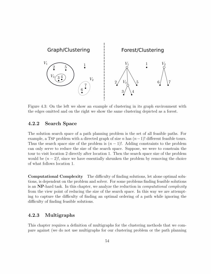
Forest/ClusteringGraph/Clustering

Figure 4.3: On the left we show an example of clustering in its graph environment withthe edges omitted and on the right we show the same clustering depicted as a forest.

4.2.2 Search Space

The solution search space of a path planning problem is the set of all feasible paths. Forexample, a TSP problem with a directed graph of size n has (n−1)! different feasible tours.Thus the search space size of the problem is (n − 1)!. Adding constraints to the problemcan only serve to reduce the size of the search space. Suppose, we were to constrain thetour to visit location 2 directly after location 1. Then the search space size of the problemwould be (n− 2)!, since we have essentially shrunken the problem by removing the choiceof what follows location 1.

Computational Complexity The difficulty of finding solutions, let alone optimal solu-tions, is dependent on the problem and solver. For some problems finding feasible solutionsis an NP-hard task. In this chapter, we analyze the reduction in computational complexityfrom the view point of reducing the size of the search space. In this way we are attempt-ing to capture the difficulty of finding an optimal ordering of a path while ignoring thedifficulty of finding feasible solutions.

4.2.3 Multigraphs

This chapter requires a definition of multigraphs for the clustering methods that we com-pare against (we do not use multigraphs for our clustering problem or the path planning

54

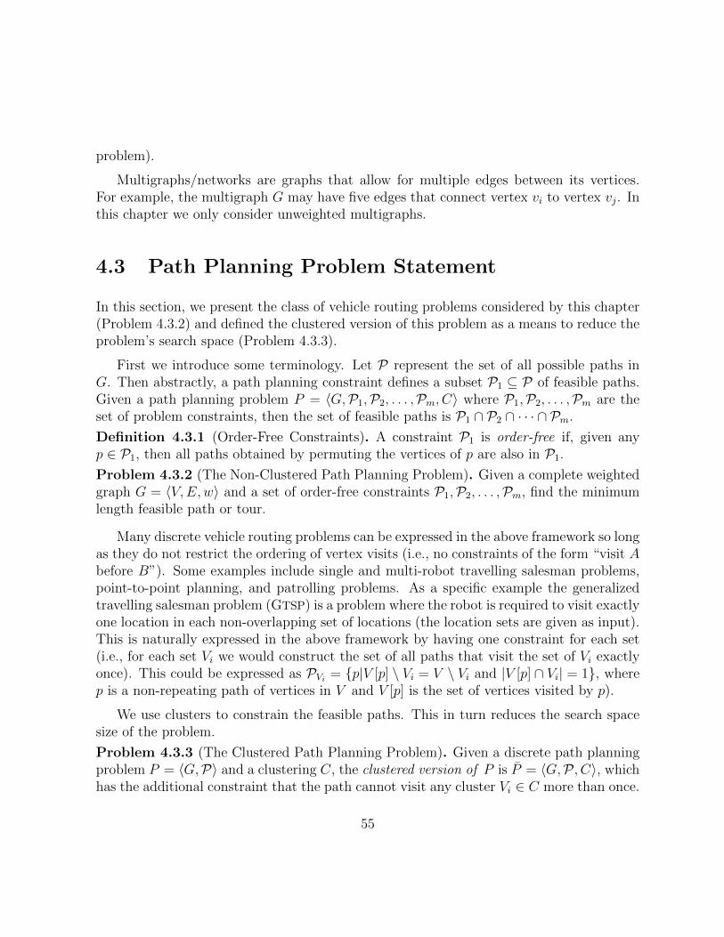
problem).

Multigraphs/networks are graphs that allow for multiple edges between its vertices.For example, the multigraph G may have five edges that connect vertex vi to vertex vj. Inthis chapter we only consider unweighted multigraphs.

4.3 Path Planning Problem Statement

In this section, we present the class of vehicle routing problems considered by this chapter(Problem 4.3.2) and defined the clustered version of this problem as a means to reduce theproblem’s search space (Problem 4.3.3).

First we introduce some terminology. Let P represent the set of all possible paths inG. Then abstractly, a path planning constraint defines a subset P1 ⊆ P of feasible paths.Given a path planning problem P = 〈G,P1,P2, . . . ,Pm, C〉 where P1,P2, . . . ,Pm are theset of problem constraints, then the set of feasible paths is P1 ∩ P2 ∩ · · · ∩ Pm.

Definition 4.3.1 (Order-Free Constraints). A constraint P1 is order-free if, given anyp ∈ P1, then all paths obtained by permuting the vertices of p are also in P1.

Problem 4.3.2 (The Non-Clustered Path Planning Problem). Given a complete weightedgraph G = 〈V,E,w〉 and a set of order-free constraints P1,P2, . . . ,Pm, find the minimumlength feasible path or tour.

Many discrete vehicle routing problems can be expressed in the above framework so longas they do not restrict the ordering of vertex visits (i.e., no constraints of the form “visit Abefore B”). Some examples include single and multi-robot travelling salesman problems,point-to-point planning, and patrolling problems. As a specific example the generalizedtravelling salesman problem (GTSP) is a problem where the robot is required to visit exactlyone location in each non-overlapping set of locations (the location sets are given as input).This is naturally expressed in the above framework by having one constraint for each set(i.e., for each set Vi we would construct the set of all paths that visit the set of Vi exactlyonce). This could be expressed as PVi = p|V [p] \ Vi = V \ Vi and |V [p] ∩ Vi| = 1, wherep is a non-repeating path of vertices in V and V [p] is the set of vertices visited by p).

We use clusters to constrain the feasible paths. This in turn reduces the search spacesize of the problem.

Problem 4.3.3 (The Clustered Path Planning Problem). Given a discrete path planningproblem P = 〈G,P〉 and a clustering C, the clustered version of P is P = 〈G,P , C〉, whichhas the additional constraint that the path cannot visit any cluster Vi ∈ C more than once.

55

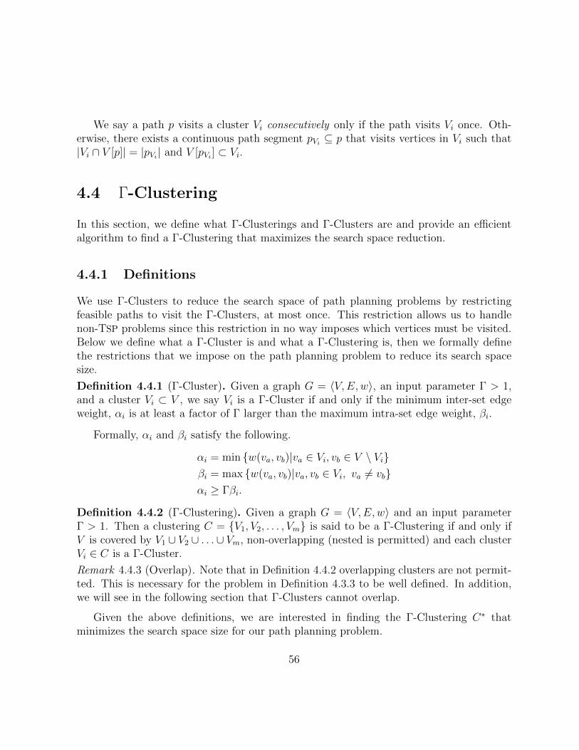
We say a path p visits a cluster Vi consecutively only if the path visits Vi once. Oth-erwise, there exists a continuous path segment pVi ⊆ p that visits vertices in Vi such that|Vi ∩ V [p]| = |pVi | and V [pVi ] ⊂ Vi.

4.4 Γ-Clustering

In this section, we define what Γ-Clusterings and Γ-Clusters are and provide an efficientalgorithm to find a Γ-Clustering that maximizes the search space reduction.

4.4.1 Definitions

We use Γ-Clusters to reduce the search space of path planning problems by restrictingfeasible paths to visit the Γ-Clusters, at most once. This restriction allows us to handlenon-TSP problems since this restriction in no way imposes which vertices must be visited.Below we define what a Γ-Cluster is and what a Γ-Clustering is, then we formally definethe restrictions that we impose on the path planning problem to reduce its search spacesize.

Definition 4.4.1 (Γ-Cluster). Given a graph G = 〈V,E,w〉, an input parameter Γ > 1,and a cluster Vi ⊂ V , we say Vi is a Γ-Cluster if and only if the minimum inter-set edgeweight, αi is at least a factor of Γ larger than the maximum intra-set edge weight, βi.

Formally, αi and βi satisfy the following.

αi = min w(va, vb)|va ∈ Vi, vb ∈ V \ Viβi = max w(va, vb)|va, vb ∈ Vi, va 6= vbαi ≥ Γβi.

Definition 4.4.2 (Γ-Clustering). Given a graph G = 〈V,E,w〉 and an input parameterΓ > 1. Then a clustering C = V1, V2, . . . , Vm is said to be a Γ-Clustering if and only ifV is covered by V1 ∪ V2 ∪ . . .∪ Vm, non-overlapping (nested is permitted) and each clusterVi ∈ C is a Γ-Cluster.

Remark 4.4.3 (Overlap). Note that in Definition 4.4.2 overlapping clusters are not permit-ted. This is necessary for the problem in Definition 4.3.3 to be well defined. In addition,we will see in the following section that Γ-Clusters cannot overlap.

Given the above definitions, we are interested in finding the Γ-Clustering C∗ thatminimizes the search space size for our path planning problem.

56

Problem 4.4.4 (The Clustering Problem). Given a path planning problem P = 〈G,P〉and a parameter Γ > 1, find a Γ-Clustering C∗ of G such that the search space size of theclustered problem P is minimized.

Note 4.4.5. Γ-Clusters are found within the environment, not imposed onto the environ-ment. As such some problems have many Γ-Clusters while others, little to none. Addi-tionally, a larger choice of Γ will tend to result in a Γ-Clustering with fewer Γ-Clustersand for some sufficiently large choice of Γ there will be no non-trivial (of size two or more)Γ-Clusters to be found within the environment.

The methods presented in this chapter rely on finding Γ-Clusters, as such problemsthat contain Γ-Clusters will benefit from these approaches. Furthermore, it has been ourexperience that most path planning environments contain Γ-Clusters (see Section 4.8).

4.4.2 Finding Γ-Clusters

Based on Problem 4.3.3 and Problem 4.4.4, the task of finding a maximal clustering comesdown to finding a clustering C∗ that contains as many clusters as possible. Each clusteradds more constraints to the problem and can only serve to reduce the problem’s searchspace size — at worst, it stays the same size. In this section we show that there exists aunique maximal set C∗ and that all other Γ-Clusterings are a subset of C∗. We provide anefficient algorithm based on MSTs to calculate C∗. Below is a series of properties that weleverage in the algorithm.

Overlap

A special property of Γ-Clustering is that there are no overlapping clusters. Specifically,there are no two clusters Vi and Vj that have a non-zero intersection unless one cluster isnested within the other.

Lemma 4.4.6. Given a graph G and Γ-Clusters Vi and Vj with Γ > 1, then Vi and Vj donot overlap.

Proof. We prove the above result by contradiction. Before we begin, recall that edges cutby the cluster Vi have edge weights ≥ αi and edges within the cluster have edge weights≤ βi. Let us assume that Vi and Vj overlap but are not nested. Without loss of generalitylet βj ≤ βi. Then there exists an edge 〈va, vb〉 with weight w(va, vb) ≤ βj for va ∈ Vi ∩ Vjand vb ∈ Vj \ (Vi ∩ Vj). Since this edge does not exist in the cluster Vi and it is cut byVi, then it must be the case that w(va, vb) ≥ αi. However, this edge does exist in the

57

cluster Vj and so αi ≤ βj, since w(va, vb) ≤ βj. This result highlights the contradiction:αiβi≤ βj

βi≤ βi

βi= 1.

Uniqueness

The non-overlapping property for Γ-Clusterings implies that there exists a unique maximalΓ-Clustering C∗ (more clusters equates to more reductions in the search space size). Thisresult follows from the simple property that if a Γ-Cluster Vi exists and is not in ourclustering C∗, then we can add it to C∗ to obtain additional search space reductions.

Proposition 4.4.7. Given graph G and a parameter Γ > 1, the problem of finding aΓ-Clustering C∗ that maximizes the search space reduction has a unique solution C∗.Furthermore C∗ contains all clusters Vi with separation αi ≥ Γβi.

Proof. We use contradiction to prove that C∗ is unique. Suppose there exists two differentΓ-Clusterings C1 and C2 that maximize the search space reductions for a Γ > 1. Therefore,there is a cluster V1 that is in C1 but not in C2 (or vice versa). This implies that either V1

is somehow incompatible with C2, which we know is not the case due to Lemma 4.4.6 (i.e.,clusters do not overlap unless one is a subset of the other) or this cluster can be added toC2. This is a contradiction that proves the first result. The second result directly followssince adding a cluster can only further reduce the search space size of the problem.

Corollary 4.4.8. Given a graph G = 〈V,E,w〉 and two optimal Γ-Clusterings C∗i and C∗jsuch that Γj > Γi > 1, then C∗j ⊆ C∗i .

Proof. We prove this result by contradiction. Suppose we have a cluster V1 ∈ C∗j that isnot in C∗i . By the definition α1 ≥ Γjβ1, where α1 is the minimum inter-set edge weightfor V1 and β1 is the maximum intra-set edge weight of V1. Since Γj > Γi then α1 ≥ Γiβ1,which implies that V1 could be in C∗i . This contradicts Proposition 4.4.7, which states thatall clusters that could be in the optimal clustering are in the optimal clustering. Therefore,if Γj > Γi > 1, then C∗j ⊆ C∗i .

Corollary 4.4.9. There exists a minimum Γ∗ > 1 and its optimal Γ-Clustering C∗ thatacts as a superset for all other Γ-Clusterings.

Proof. We prove this result by contradiction. Suppose, we have Γ∗ and C∗. Then assume,there exists a Γ > Γ∗ with a Γ-Clustering C that is a superset of C∗. Corollary 4.4.8 statesthat C ⊆ C∗, which highlights the contradiction. Additionally, every graph has a finitenumber of clusters. Therefore, there must exist a minimum value of Γ∗ > 1 that finds theΓ-Clustering C∗ that is a superset of all other Γ-Clusters.

58

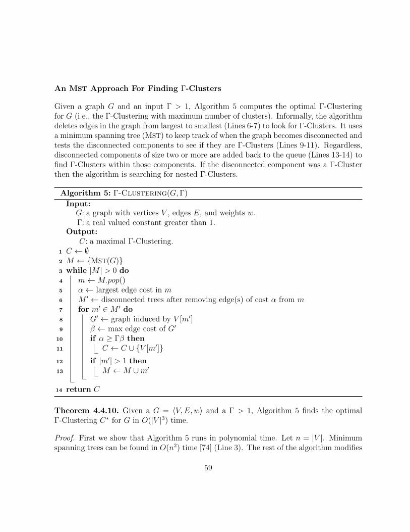
An MST Approach For Finding Γ-Clusters

Given a graph G and an input Γ > 1, Algorithm 5 computes the optimal Γ-Clusteringfor G (i.e., the Γ-Clustering with maximum number of clusters). Informally, the algorithmdeletes edges in the graph from largest to smallest (Lines 6-7) to look for Γ-Clusters. It usesa minimum spanning tree (MST) to keep track of when the graph becomes disconnected andtests the disconnected components to see if they are Γ-Clusters (Lines 9-11). Regardless,disconnected components of size two or more are added back to the queue (Lines 13-14) tofind Γ-Clusters within those components. If the disconnected component was a Γ-Clusterthen the algorithm is searching for nested Γ-Clusters.

Algorithm 5: Γ-Clustering(G,Γ)

Input:G: a graph with vertices V , edges E, and weights w.Γ: a real valued constant greater than 1.

Output:C: a maximal Γ-Clustering.

1 C ← ∅2 M ← MST(G)3 while |M | > 0 do4 m←M.pop()5 α← largest edge cost in m6 M ′ ← disconnected trees after removing edge(s) of cost α from m7 for m′ ∈M ′ do8 G′ ← graph induced by V [m′]9 β ← max edge cost of G′

10 if α ≥ Γβ then11 C ← C ∪ V [m′]12 if |m′| > 1 then13 M ←M ∪m′

14 return C

Theorem 4.4.10. Given a G = 〈V,E,w〉 and a Γ > 1, Algorithm 5 finds the optimalΓ-Clustering C∗ for G in O(|V |3) time.

Proof. First we show that Algorithm 5 runs in polynomial time. Let n = |V |. Minimumspanning trees can be found in O(n2) time [74] (Line 3). The rest of the algorithm modifies

59

the MST found in Line 3, which originally has n edges. Thus the while loop for the restof the algorithm runs at most n times (we can’t remove more than n edges). Finding thelargest edge(s) and removing them in Line 6 and 7 takes O(n) time. Creating the inducedsubgraph and finding the maximum edge cost in Lines 9 and 10 takes O(n2) time. Testingif the subgraph is a clique (Line 11) takes O(n2) time. Thus Lines 1-3 run in O(n2) timeand Lines 4-14 run in O(n·n2), meaning the entire algorithm runs in O(n3) time or O(|V |3).

Next, we show that Algorithm 5 finds the optimal Γ-Clustering. To do so, we showthat each V [m′] found in Line 11 is a Γ-Cluster as defined by Definition 4.4.1. Then weshow that the algorithm does not omit any candidate clusters.

Let us start by understanding how MSTs are used to find Γ-Clusters. A Γ-Cluster withseparation Γ > 1 is a subgraph of G that is connected with intra-edge weights less thanthe inter-edge weights. Let α be the minimum edge weight connected to the subgraph(minimum inter-edge weight) and β be the maximum edge weight within the subgraph(maximum intra-edge weight). Thus one method of searching for Γ-Clusters is to deleteall edges of weight ≥ α in the graph and test the disconnected components (subgraphs).We can use MSTs to efficiently keep track of these deleted edges. By definition, an MST

is a tree that connects vertices within the graph with minimum edge weight. When weremove edges of size ≥ α to search for disconnected subgraphs, the graph is disconnectedif and only if the MST is disconnected (the cut that disconnects the graph also disconnectsthe MST). Furthermore, the algorithm incrementally removes the edge(s) in the MST fromlargest to smallest so that we can emulate removing edges in the graph of cost ≥ α. Thusif the induced subgraph G′ created in Line 9 has a maximum intra-edge weight of β, thenit is a Γ-Cluster if α ≥ Γβ. For these reasons it is added to the clustering C in Line 12.

Now, we show that the Algorithm does not omit any candidate clusters. We havealready argued that only disconnected MST trees need to be considered for Γ-Clusters.What is left to show is that the algorithm tests every possible value of α for disconnectingthe MST tree. This is true since it considers every edge in the MST. Thus every candidatecluster of size two or more is considered.

Therefore, this algorithm finds all of the candidate Γ-Clusters and Proposition 4.4.7implies that this clustering is the unique optimal Γ-Clustering for the given Γ > 1.

4.5 Coupled Planning

In this section we solve the clustered problem P instead of the non-clustered problem P(Problem 4.3.3 and Problem 4.3.2 respectively). We show that the clustered problem can

60

have a search space size that is exponentially smaller than the non-clustered problem. Wealso show that the cost c∗ of optimal solutions of P are within a constant factor of c∗,where c∗ is the cost of optimal solutions for P .

4.5.1 Search Space Reduction

The task of measuring the reduction in search space size from Problem P to P for aclustering C, depends on the set of feasible paths for P and C. For our analysis, we studythe reduction of search space size for the path planning problem TSP. This problem’s setof feasible paths are all tours that visit each vertex exactly once. Thus the size of thesearch space for this problem is

N0 = (|V | − 1)!.

The size of the clustered problem’s search space (Problem 4.3.3) is

N1 = (|Roots(C)| − 1)!∏Vi∈C

|Children(Vi)|!,

where the function Roots(C) returns the root clusters of C and the function Children(Vi)returns the children of Vi (see Section 4.2.1 for the definition of roots and children).

Note 4.5.1. The functions Roots and Children, return a set of sets instead of a hybridof sets and vertices. We do this to simplify the algorithms within this chapter.

To simplify the analysis, we study clusterings that contain m equally sized clusters ofsize x = |V |/m, where x ∈ Z. Now we have

N1 = (m− 1)!m∏i=1

x!.

Lemma 4.5.2. Given |V | = mx, for m,x ∈ Z+ the following holds |V |! ≥ m!xx!m.

61

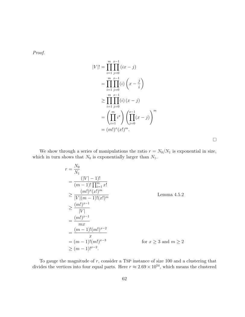
Proof.

|V |! =m∏i=1

x−1∏j=0

(ix− j)

=m∏i=1

x−1∏j=0

(i)

(x− j

i

)

≥m∏i=1

x−1∏j=0

(i) (x− j)

=

(m∏i=1

ix

)(x−1∏j=0

(x− j)

)m

= (m!)x(x!)m.

We show through a series of manipulations the ratio r = N0/N1 is exponential in size,which in turn shows that N0 is exponentially larger than N1.

r =N0

N1

=(|V | − 1)!

(m− 1)!∏m

i=1 x!

≥ (m!)x(x!)m

|V |(m− 1)!(x!)mLemma 4.5.2

≥ (m!)x−1

|V |

=(m!)x−1

mx

=(m− 1)!(m!)x−2

x= (m− 1)!(m!)x−3 for x ≥ 3 and m ≥ 2

≥ (m− 1)!x−2.

To gauge the magnitude of r, consider a TSP instance of size 100 and a clustering thatdivides the vertices into four equal parts. Here r ≈ 2.69× 1054, which means the clustered

62

problem has search space that is more than 1054 smaller than the non-clustered problem’ssearch space. However N1 is still extremely large, N1 ≈ 3.47× 10101.

4.5.2 Solution Quality Bounds

In this section, we show that when P = 〈G,P〉 is metric (the graph G is metric) thesolutions to the clustered problem P = 〈G,P , C〉 have cost c bound by

c∗ ≤ min

(2,

(1 +

3

2Γ

))c∗,

where c∗ is the optimal cost of P . We start by proving the first half of the result (c∗ ≤ 2c∗).We do this with a series of theoretical results that use minimum spanning trees (MST) toconstruct feasible solutions.

Lemma 4.5.3. Given a metric graph G and a Γ-Clustering C with Γ > 1, then every MST

will have exactly one inter-set edge for each cluster Vi ∈ C.

Proof. We prove the above result by contradiction. Suppose the MST has at least twointer-set edges connected to Vi. Thus, there are at least two sets of vertices in Vi that arenot connected to each other using intra-set edges. We can lower the cost of the MST byremoving one of these inter-set edges of weight ≥ αi and replace it with an intra-set edgeof weight ≤ βi < αi. This highlights the contradiction. Therefore, every MST will haveexactly one inter-set edge for each Γ-Cluster Vi ∈ C.

Lemma 4.5.4 (Two-Factor Approximation). Consider a metric discrete path planningproblem P with an optimal solution path p∗ and cost c∗. Then given a Γ-ClusteringC = V1, V2, . . . , Vm with Γ > 1, the optimal solution p∗ for the clustered problem P overthe same set of vertices V [p∗] is a solution to P with cost c∗ ≤ 2c∗.

Proof. To prove the above result, we use the MST approach described below and in [49] toconstruct a path p over the set of vertices in V [p∗]. This approach yields a solution p forP that has the desired cost bound, c ≤ 2c∗ [49]. The MST procedure is described below.

1. Find a minimum spanning tree for the vertices V [p∗].

2. Duplicate each edge in the tree to create a Eulerian graph.

3. Find an Eulerian tour of the Eulerian graph.

63

4. Convert the tour to a TSP: if a vertex vi is visited more than once after the firstvisit, create a shortcut: from the vertex before vi to the vertex after vi (i.e., create atour that visits the vertices in the order they first appeared in the tour).

What remains to prove is that the above tour is a feasible solution for P . First we notethat the above approach yields a single tour of all the vertices in V [p∗] (i.e., there are nodisconnected tours). Note that Lemma 4.5.3 states that every MST uses exactly one inter-set edge for each cluster Vi ∈ C. Thus when the edges are duplicated and a Eulerian touris found, there are only two inter-set edges used for each Vi ∈ C. Furthermore shortcuttingthe path does not change the number of inter-set edges used by the tour, thus the finalsolution p only has one incoming and one outgoing edge for each cluster Vi ∈ C. As aresult it is a clustered solution for P that satisfies the bound since the MST approach alsoyields a solution with cost c ≤ 2c∗.

Next, we prove the second half of the bound c∗ ≤(1 + 3

2Γ

)c∗ by using Algorithm 6

to construct p (a feasible solution for P ). Additionally, we use a modified graph (Defini-tion 4.5.8) to show that the cost of the solution satisfies our desired bound.

Lemma 4.5.5 (Correctness of Algorithm 6). Given a feasible path p for P and a clusterVi ∈ C that is not visited consecutively, then p′ ← Deform(p, Vi) visits Vi consecutivelyand any subsequent deformed paths also visits Vi consecutively.

Proof. By construction, Vi is visited consecutively in p′ ← Deform(p, Vi). The remainingclaim that Vi continues to be visited consecutively is proven by showing that the set ofintra-set edges for Vi remains unchanged.

We prove this result by contradiction. Suppose, there exists some deformed path p′′′

that came some time after p′, such that the edge 〈va, vb〉 ∈ p′ for some va, vb ∈ Vi but notin p′′ (〈va, vb〉 6∈ p′′). Furthermore, let p′′′ be the first deformed path that does not havethis edge and let p′′′ ← Deform(p′′, Vj) be the path before the deformation.

This means that Algorithm 6 inserts one or more vertices in between va and vb. Thiscannot happen in Lines 5-7 since the path for the 1st vertex to the kth is unchanged. Alsothis cannot happen in Lines 8-9 since this part of the algorithm is only connecting verticeswithin the cluster Vj together. Finally, this cannot happen in Lines 11-13, since the pathis not changing the order of the appearance of va and vb (no insertions, just deletions).

Thus 〈va, vb〉 must be in p′′′, which highlights the contradiction. Therefore, all subse-quent paths must also visit Vi consecutively, since all intra-set edges remain intact.

64

Algorithm 6: Deform(p, Vi)

Input:p: a path represented as an array.Vi: a cluster.

Output:p: a deformed path that visits Vi at most once.

1 if p has two or less inter-set edges for Vi then2 return p

3 k ← 14 p← [ ] /* empty array */

5 while p[k] 6∈ Vi do6 p.append(p[k])7 k ← k + 1

8 for l ∈ [k, k + 1, . . . , |p|] do9 if p[l] ∈ Vi then

10 p.append(p[l])

11 for l ∈ [k, k + 1, . . . , |p|] do12 if p[l] 6∈ Vi then13 p.append(p[l])

14 return p

65

Remark 4.5.6 (Uniqueness). When Algorithm 6 is applied to p∗ iteratively for each Vi ∈ Cto generate the solution p, the solution is unique despite the order that Deform(p, Vi) wascalled. Furthermore the order of the clusters is determined by their first appearance in p.

This is how Algorithm 6 reorders the vertices within the tour. Specifically, the orderof vertices within each cluster Vi is preserved as deform(p, Vi) is called, as well as theordering of the remaining vertices.

Lemma 4.5.7 (Deformation cost). Consider a feasible path p for P that has 2(n+ 1) ≥ 4inter-set edges for Γ-Cluster Vi such that Γ > 1 and n ∈ Z≥0. Then the cost to deform pinto p← Deform(p, Vi) is c− c ≤ (2n+ 1)βi.

Proof. We analyze the cost to deform p into p for each type of deformation the algorithmuses.: There are three types of deformations: 1) shortcuts are created within the cluster;2) shortcuts are created outside of the cluster; and 3) the cluster adopts a new outgoingedge. These deformations are illustrated in Figure 4.4. A classification of the edges in thefigure are as follows: 1) edges 〈v3, v4〉 and 〈v6, v7〉 are shortcuts within the cluster; 2) edges〈v10, v11〉 and 〈v12, v13〉 are shortcuts outside of the cluster; and 3) edge 〈v8, v9〉 is the newoutgoing edge for the cluster.

We start by examining the incurred cost to shortcut paths within the cluster. Considera path segment 〈va, vb, vc, . . . , vx, vy, vz〉 of p such that va is directly connected to vz in pwith the edge 〈va, vz〉 and va, vz ∈ Vi. The incurred cost of each of these edges is ≤ βi dueto the fact that the cost of any intra-set edge has weight ≤ βi. There are n such shortcutsof this nature incurred from Deform(p, Vi) (n captures the number of extra visits to thecluster) and so the total incurred cost for this type of shortcut is ≤ nβi.

Next, we examine the incurred cost to shortcut paths outside of the cluster. Considera path segment 〈va, vb, vc, . . . , vx, vy, vz〉 of p such that va is directly connected to vz inp with the edge 〈va, vz〉, va, vz 6∈ Vi and vb, vc, . . . , vy ∈ Vi. The incurred cost for eachof these shortcuts is again ≤ βi. This is due to the metric property of G. The cost ofthe direct path from va to vz is less than or equal to any path from va to vz, specificallyc(va, vz) ≤ c(va, vb) + c(vb, vy) + c(vy, vz) ≤ c(va, vb) +βi+ c(vy, vz). Thus the incurred cost,∆, of this shortcut is bound by the difference between the cost of the new edges in p andthe removed edges in p∗, namely:

∆ = c(va, vz)− c(va, vb)− c(vy, vz)≤ c(va, vb) + βi + c(vy, vz)− c(va, vb)− c(vy, vz)≤ βi.

66

There are n such shortcuts of this nature incurred by Deform(p, Vi). Thus, the totalincurred cost for this type of shortcut is also ≤ nβi.

Lastly we examine the incurred cost of the new outgoing edge. Consider the path〈va, vb, vc, . . . , vx, vy, vz〉 of p such that 〈vb, vc〉 is the first outgoing edge of Vi and 〈vx, vy〉is the last outgoing edge of Vi, thus 〈vx, vc〉 is the new outgoing edge. Then due to themetric property we know that c(vx, vc) ≤ c(vx, vb) + c(vb, vc) ≤ βi + c(vb, vc). The incurredcost, ∆, of this deformation is the difference between the cost of the new edge 〈vx, vc〉 andthe removed edge 〈vb, vc〉 (this edge has not been considered in any previous incurred costcalculation):

∆ = c(vx, vc)− c(vb, vc)≤ βi + c(vb, vc)− c(vb, vc)≤ βi.

This accounts for all the incurred costs, and so the total cost to deform p into p viaDeform(p, Vi) is c− c ≤ (2n+ 1)βi.

We introduce the modified graph G in the following definition to aid with our ongoingproof of the bound.

Definition 4.5.8 (The modified graph G). Given a graph G and a Γ-Clustering C, themodified graph G is a copy of G with the following modifications: if 〈va, vb〉 is an inter-set edge with va ∈ Vi and vb ∈ Vj, then w(va, vb) = w(va, vb) + 3

2max(βi, βj); otherwise

w(va, vb) = w(va, vb), where βi and βj are defined as in Definition 4.4.1.

Lemma 4.5.9 (Deformation cost in G). Consider a feasible path p for P , a Γ-Cluster Viwith Γ > 1, and p ← Deform(p, Vi), then the cost of p and p in G satisfies c(p) ≤ c(p),where c(p) and c(p) are the cost of p and p in G respectively. In other words the cost todeform p into p is ≤ 0 for G.

Proof. In this proof we analyze the cost to deform p into p in G, which is a result of singlecall p← Deform(p, Vi) (Algorithm 6).

From Lemma 4.5.7, we see that the cost to deform p into p with respect to G isc− c ≤ (2n + 1)βi, where there are 2(n + 1) ≥ 4 inter-set edges for Vi in p. The cost of pin G is

c(p) ≥ c+ 2(n+ 1)

(3

2

)βi = c+ 3(n+ 1)βi

67

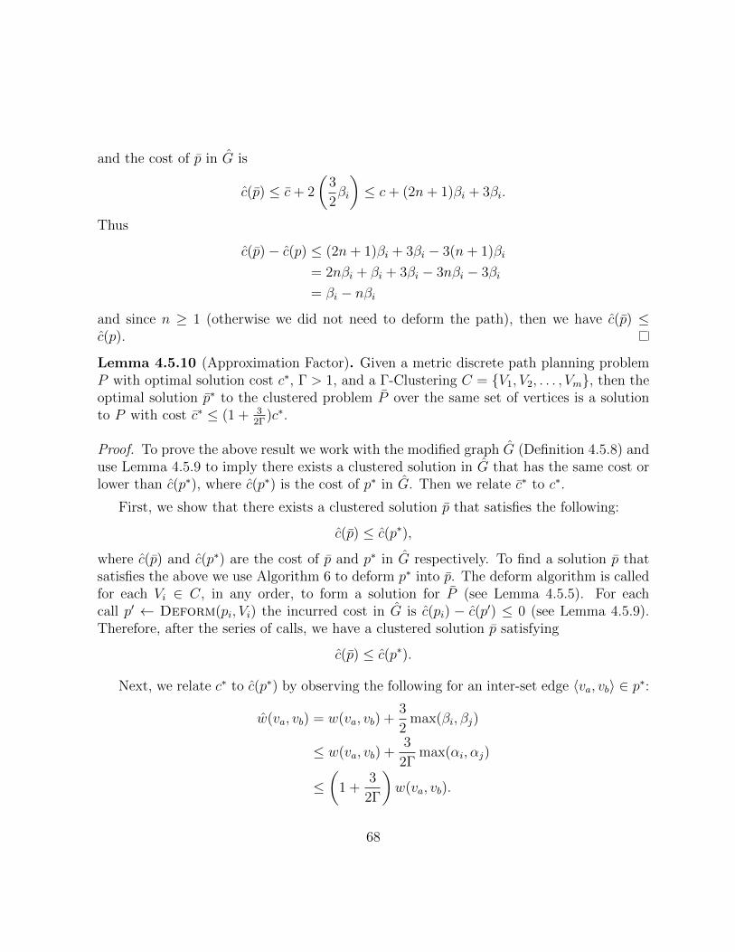
and the cost of p in G is

c(p) ≤ c+ 2

(3

2βi

)≤ c+ (2n+ 1)βi + 3βi.

Thus

c(p)− c(p) ≤ (2n+ 1)βi + 3βi − 3(n+ 1)βi

= 2nβi + βi + 3βi − 3nβi − 3βi

= βi − nβiand since n ≥ 1 (otherwise we did not need to deform the path), then we have c(p) ≤c(p).

Lemma 4.5.10 (Approximation Factor). Given a metric discrete path planning problemP with optimal solution cost c∗, Γ > 1, and a Γ-Clustering C = V1, V2, . . . , Vm, then theoptimal solution p∗ to the clustered problem P over the same set of vertices is a solutionto P with cost c∗ ≤ (1 + 3

2Γ)c∗.

Proof. To prove the above result we work with the modified graph G (Definition 4.5.8) anduse Lemma 4.5.9 to imply there exists a clustered solution in G that has the same cost orlower than c(p∗), where c(p∗) is the cost of p∗ in G. Then we relate c∗ to c∗.

First, we show that there exists a clustered solution p that satisfies the following:

c(p) ≤ c(p∗),

where c(p) and c(p∗) are the cost of p and p∗ in G respectively. To find a solution p thatsatisfies the above we use Algorithm 6 to deform p∗ into p. The deform algorithm is calledfor each Vi ∈ C, in any order, to form a solution for P (see Lemma 4.5.5). For eachcall p′ ← Deform(pi, Vi) the incurred cost in G is c(pi) − c(p′) ≤ 0 (see Lemma 4.5.9).Therefore, after the series of calls, we have a clustered solution p satisfying

c(p) ≤ c(p∗).

Next, we relate c∗ to c(p∗) by observing the following for an inter-set edge 〈va, vb〉 ∈ p∗:

w(va, vb) = w(va, vb) +3

2max(βi, βj)

≤ w(va, vb) +3

2Γmax(αi, αj)

≤(

1 +3

2Γ

)w(va, vb).

68

The above inequality is true for each edge 〈va, vb〉 ∈ p∗, inter-set edge or not. Thereforethe path cost satisfies

c(p∗) ≤(

1 +3

2Γ

)c∗.

Due to the construction of G and how c(p) ≤ c(p∗) we deduce that

c∗ ≤ c(p∗),

sincec∗ ≤ c(p) ≤ c(p) ≤ c(p∗),

where c(p) is the cost of p in G. Therefore

c∗ ≤(

1 +3

2Γ

)c∗.

Theorem 4.5.11 (Approximation Factor). Given a metric discrete path planning problemP , an optimal solution p∗ with cost c∗, and a Γ-Clustering C = V1, V2, . . . , Vm with Γ > 1,then the optimal solution p∗ to the clustered problem P over the same set of vertices is asolution to P with cost c∗ ≤ min

(2, 1 + 3

2Γ

)c∗.

Proof. The proof directly follows from Lemma 4.5.4 and Lemma 4.5.10.

Remark 4.5.12 (Tightness of Bound). To better characterize the tightness of the boundprovided by Theorem 4.5.11, we provide a lower bound for the solution quality of solvingP instead of P (Problem 4.3.3 and Problem 4.3.2 respectively). Additionally, Figure 4.6visualizes the gap between the lower and upper bound for increasing values of Γ.

The lower bound problem is illustrated in Figure 4.5. In this example, the graph isscalable (add three vertices at a time). The clustered and non-clustered solutions for thisexample have a cost relation of

lim|V |→∞

c∗ =

(1 +

2

2Γ + 1

)c∗.

69

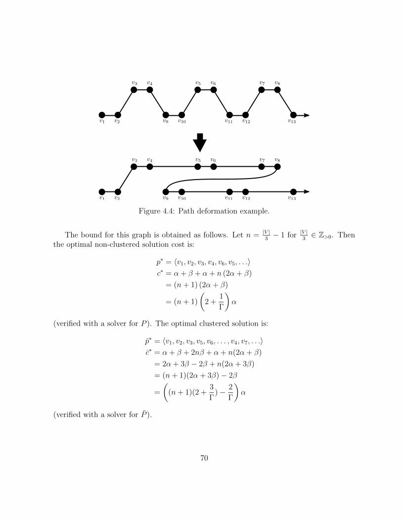
Figure 4.4: Path deformation example.

The bound for this graph is obtained as follows. Let n = |V |3− 1 for |V |

3∈ Z>0. Then

the optimal non-clustered solution cost is:

p∗ = 〈v1, v2, v3, v4, v6, v5, . . .〉c∗ = α + β + α + n (2α + β)

= (n+ 1) (2α + β)

= (n+ 1)

(2 +

1

Γ

)α

(verified with a solver for P ). The optimal clustered solution is:

p∗ = 〈v1, v2, v3, v5, v6, . . . , v4, v7, . . .〉c∗ = α + β + 2nβ + α + n(2α + β)

= 2α + 3β − 2β + n(2α + 3β)

= (n+ 1)(2α + 3β)− 2β

=

((n+ 1)(2 +

3

Γ)− 2

Γ

)α

(verified with a solver for P ).

70

Optimal Clustered Solution:

Optimal Solution:

Figure 4.5: Metric example instance (α > β). Vertices in the top row (v2, v3, v5, v6, . . .)are in the cluster Vi. Edge weights connecting vertices within Vi are β. Edge weightsconnecting vertices not in Vi are 2α + β. Edge weights connecting vertices not in Vi tovertices in Vi are α + β, unless shown differently in diagram.

As the instance grows (|V | → ∞ and n→∞), we have the following:

limn→∞

c∗ =(n+ 1)

(2 + 3

Γ

)− 2

Γ

(n+ 1)(2 + 1

Γ

) c∗

=

(2 + 3

Γ

2 + 1Γ

)c∗

=

(1 +

2

2Γ + 1

)c∗,

which confirms the stated bound.

71

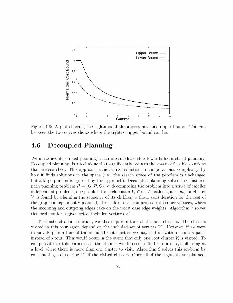
1

1.2

1.4

1.6

1.8

2

2.2

1 2 3 4 5 6 7 8 9 10

Nor

mal

ized

Cos

t Bou

nd

Gamma

Upper BoundLower Bound

Figure 4.6: A plot showing the tightness of the approximation’s upper bound. The gapbetween the two curves shows where the tightest upper bound can lie.

4.6 Decoupled Planning

We introduce decoupled planning as an intermediate step towards hierarchical planning.Decoupled planning, is a technique that significantly reduces the space of feasible solutionsthat are searched. This approach achieves its reduction in computational complexity, byhow it finds solutions in the space (i.e., the search space of the problem is unchangedbut a large portion is ignored by the approach). Decoupled planning solves the clusteredpath planning problem P = 〈G,P , C〉 by decomposing the problem into a series of smallerindependent problems, one problem for each cluster Vi ∈ C. A path segment pVi for clusterVi is found by planning the sequence of its children without consideration for the rest ofthe graph (independently planned). Its children are compressed into super vertices, wherethe incoming and outgoing edges take on the worst case edge weights. Algorithm 7 solvesthis problem for a given set of included vertices V ′.

To construct a full solution, we also require a tour of the root clusters. The clustersvisited in this tour again depend on the included set of vertices V ′. However, if we wereto naıvely plan a tour of the included root clusters we may end up with a solution path,instead of a tour. This would occur in the event that only one root cluster Vi is visited. Tocompensate for this corner case, the planner would need to find a tour of Vi’s offspring ata level where there is more than one cluster to visit. Algorithm 9 solves this problem byconstructing a clustering C ′ of the visited clusters. Once all of the segments are planned,

72

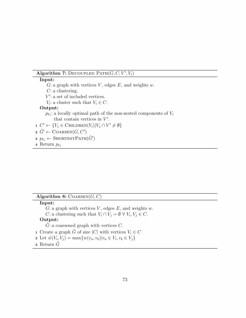
Algorithm 7: Decoupled Path(G,C, V ′, Vi)

Input:G: a graph with vertices V , edges E, and weights w.C: a clustering.V ′: a set of included vertices.Vi: a cluster such that Vi ∈ C.

Output:pVi : a locally optimal path of the non-nested components of Vi

that contain vertices in V ′.

1 C ′ ← Vj ∈ Children(Vi)|Vj ∩ V ′ 6= ∅2 G′ ← Coarsen(G,C ′)

3 pVi ← ShortestPath(G′)4 Return pVi

Algorithm 8: Coarsen(G,C)

Input:G: a graph with vertices V , edges E, and weights w.C: a clustering such that Vi ∩ Vj = ∅ ∀ Vi, Vj ∈ C.

Output:G: a coarsened graph with vertices C.

1 Create a graph G of size |C| with vertices Vi ∈ C2 Let w(Vi, Vj) = maxw(va, vb)|va ∈ Vi, vb ∈ Vj3 Return G

73

then a full solution is constructed by recursively replacing the super vertices Vi in the tourwith their corresponding path segments pVi .

Decoupled planning can also be used to find solutions for P without the knowledge ofV ′. This is accomplished by re-coupling the smaller problems back together with someadditional logic to ensure that a solution tour is found instead of a path. Then the re-coupled problem will find V ′, a tour of the root clusters, and a set of path segments pVi foreach visited cluster Vi. The re-coupled problem still has a much smaller search space thanP since for every feasible set V ′ the problem is finding a tour in a decoupled manner.

Algorithm 9: Decoupled Tour(G,C, V ′)

Input:G: a graph with vertices V , edges E, and weights w.C: a clustering.V ′: a set of vertices to be visited such that V ′ ⊆ V .

Output:pC : an optimal tour of the non-nested components of C

that contain vertices in V ′.

1 C ′ ← Vi ∈ C|Vi ∩ V ′ 6= ∅2 while |Roots(C ′)| = 1 do3 Replace C ′ with the root cluster Vi of C ′

4 G′ ← Coarsen(G,Roots(C ′))

5 pC ← ShortestTour(G′)6 Return pC

4.6.1 Search Space Reduction

In this section we show how decoupled planning can exponentially reduce the space ofsearched solutions. We measure this space by counting the number of feasible paths search-able by the algorithm. As with coupled planning, measuring the reduction in search spacesize depends on the set of feasible paths P for Problem 4.3.2 and the clustering C. For ouranalysis we again study the TSP problem P = 〈G,P〉, where P is the set of all tours thatvisit ever vertex in G exactly once. As before the size of the non-clustered problem is

N0 = (|V | − 1)!

74

and the size of the clustered problem’s search space (Problem 4.3.3) is

N1 = (|Roots(C)| − 1)!∏Vi∈C

|Children(Vi)|!.

The size of the space searched by the decoupled approach is

N2 = (|Roots(C)| − 1)! +∑Vi∈C

|Children(Vi)|!.

To simplify the analysis, we study clusterings C with m clusters at the top level of thehierarchy and each one of those clusters contains m clusters. This continues for total of mlevels (each cluster has m children) until each cluster in the last level contains m vertices.The search space size of this clustered problem P is

N1 = (m− 1)!m−1∏i=1

mi∏j=1

(m!) = (m− 1)!m−1∏i=1

(m!)mi

and when solved with the decoupled approach it is

N2 = (m− 1)! +m−1∑i=1

mi∑j=1

m! = (m− 1)! +m!m−1∑i=1

mi.

To show that the search space size N1 for the coupled approach is exponentially largerthan the space searched by the decoupled approach N2, we manipulate the ratio r = N1/N2

to show that it is exponential in size.

75

r =N1

N2

=(m− 1)!

∏m−1i=1 (m!)m

i

(m− 1)! +m!∑m−1

i=1 mi

≥ (m− 1)!∏m−1

i=1 (m!)mi

m!∑m−1

i=0 mi

=

∏m−1i=1 (m!)m

i

m∑m−1

i=0 mi

=

∏m−1i=1 mmi

∏m−1i=1 (m− 1)!m

i

m(mm−1m−1

)=m

∑m−1i=1 mi

∏m−1i=1 (m− 1)!m

i

m(mm−1m−1

)=mm(m

m−1m−1 )∏m−1

i=1 (m− 1)!mi

m(mm−1m−1

)≥ mm(m

m−1m−1 )∏m−1

i=1 (m− 1)!mi

mm+1

= mm(mm−1m−1 )−(m+1)

m−1∏i=1

(m− 1)!mi

≥m−1∏i=1

(m− 1)!mi

for m ≥ 2.

To get a better understanding of this size, we now consider the concrete example ofwhen m = 3. In this case there would be 27 vertices and 12 clusters (9 clusters with3 vertices and 3 clusters with 3 nested clusters). The ratio r would be approximately5.9×107, meaning the decoupled method’s search space is approximately 5.9×107 smaller.If we were to instead compare N2 to N0 then r′ = N0/N1 ≈ 5.45× 1024.

Thus the size of the space searched by the decoupled approach is exponentially smallerthan the search space of the coupled problem P and P .

76

4.6.2 Solution Quality Bounds

In this section we provide a solution quality bound for decoupled planning. We start byintroducing a modified version of the problem environment that will yield the same set ofsolutions found by the decoupled approach. Then we step through a series of theoreticalresults that are used to prove the main result, which is that solutions found with decoupledplanning have a cost c bound by c ≤ 2

(1 + 2

Γ

)c∗, where c∗ is the cost of the optimal solution

for the non-clustered path planning problem.

Definition 4.6.1 (The modified graph G). Given a graphG = 〈V,E,w〉 and a Γ-ClusteringC, we define the modified graph G = 〈V,E, w〉 as a copy of G with the following edge weightassignments. For each 〈va, vb〉 ∈ E, let Vi be the largest cluster containing va but not vband Vj be the largest cluster containing vb but not va, then w(va, vb) = maxw(vx, vy)|vx ∈Vi, vy ∈ Vj.Proposition 4.6.2. Given a metric clustered path planning problem P = 〈G,P , C〉 andits modified clustered problem P = 〈G,P , C〉, where C is a Γ-Clustering with Γ > 1 andG is the modified graph as defined in Definition 4.6.1, then the solution p obtained by thedecoupled approach is an optimal solution for P and likewise, an optimal solution p∗ forP could be obtained by the decoupled approach.

Proof. We prove the above result by showing that for every feasible set of included verticesV ′, the optimal solution p∗ could be found using the decoupled approach (with the sameset of included vertices). Let

C ′ = Vi ∩ V ′|Vi ∈ C and Vi ∩ V ′ 6= ∅

be the set of visited clusters. Let C ′0 = Roots(C ′). Let the notation p∗C′′ represent thesubset of inter-set edges between the clusters in C ′′,

〈va, vb〉 ∈ p|va ∈ V ′′i , vb ∈ V ′′j , V ′′i , V ′′j ∈ C ′′,

where C ′′ has no nested clusters.

The first property we show is that p∗C′0is a shortest tour of the root clusters of C ′ and

that p∗C′0could be equally obtained from calling Algorithm 9 with input (G,C, V ′). This

result follows from the construction of G. The costs of the edges in the tour, depend onthe sequence of the clusters in C ′0, not the choice of vertices that p∗ transitions to and fromthe root clusters. For example, if we are transitioning from V ′i to V ′j such that V ′i , V

′j ∈ C ′0

then each edge 〈va, vb〉 with va ∈ V ′i and vb ∈ V ′j has the same cost. Thus p∗C′0is a shortest

tour of the root clusters C ′0 since the cost of the tour is independent of the choice of vertices

77

transitioned within the clusters. The cost of the edges transitioning from V ′i to V ′j in G

also have equivalent cost to the coarsened graph G′ created by Algorithm 9. Thus pC fromAlgorithm 9 is a solution for p∗C′0

and vice versa since both paths are solutions for the same

problem (find a minimum cost tour of the root clusters of C ′).

For the second property, we show that for each V ′i ∈ C ′, p∗V ′iis a shortest path of

V ′i ’s children with free choice of start and goal. Alternatively, p∗V ′icould be obtained from

calling Algorithm 7 with input (G,C, V ′, Vi), where Vi ∈ C is used to construct V ′i = Vi∩V ′.This result again follows from the construction of G using the same argument as before.The choice of first and last vertices visited in V ′i is independent from the rest of the tourand the ordering of V ′i ’s children depend only on the sequence of the children (not thevertices within). Thus p∗V ′i

must also be a shortest path. Additionally in Algorithm 7, the

transition costs between the children of V ′i are equivalent to G′. Thus pVi from Algorithm 7is a solution for p∗V ′i

and vice versa since both paths are solutions for the same problem.

Therefore, to obtain p∗ one can either solve P optimally or solve P with the decoupledapproach.

Proposition 4.6.3 (Inter-set Edge Weight Bound). Given a metric graph G, its Γ-Clustering C, and any Vi, Vj ∈ C such that Vi ∩ Vj = ∅, then for any va, vx ∈ Vi, andany vb, vy ∈ Vj, the following holds: w(va, vb) ≤ (1 + 2

Γ)w(vx, vy).

Proof. The above is proven using the triangle inequality and the relations from Defini-tion 4.4.2. Specifically, we use the fact that the direct path from va to vb is no longer thanthe path from va to vx to vy to vb. Then we make a series of inequality replacements usingthe relations from Definition 4.4.2.

w(va, vb) ≤ w(va, vx) + w(vx, vy) + w(vy, vb)

≤ βi + w(vx, vy) + βj

=αiΓ

+ w(vx, vy) +αjΓ

≤ w(vx, vy)

Γ+ w(vx, vy) +

w(vx, vy)

Γ

=

(1 +

2

Γ

)w(vx, vy).

78

Lemma 4.6.4. Consider a clustered TSP problem P = 〈G,P , C〉 with optimal solution p∗

of cost c∗ and its modified clustered problem P = 〈G,P , C〉 with optimal solution p∗ ofcost c∗, then c∗ ≤

(1 + 2

Γ

)c∗.

Proof. To prove the above result we analyze the cost of p∗ in G. Let 〈va, vb〉 be an edgein p∗ and let Vi be the largest Γ-Cluster containing va but not vb and let Vj be the largestΓ-Cluster containing vb but not va (as defined in Definition 4.6.1). We use the result fromProposition 4.6.3 to bound the weight of 〈va, vb〉 in G with w(va, vb) ≤ (1 + 2

Γ)w(va, va)

and since every edge weight of p∗ is bound by a factor of (1 + 2Γ) in G, then the cost of

the entire tour p∗ must also be bound by the same factor, c(p∗) ≤ (1 + 2Γ)c∗. Therefore,

c∗ ≤ (1 + 2Γ)c∗, since c∗ represents the cost of the optimal solution of P .

Theorem 4.6.5. Given a metric planning problem P = 〈G,P〉 and a Γ-Clustering Cwith Γ > 1, then the decoupled approach will find a path p with cost c that is bound byc ≤ min(2 + 4

Γ, 1 + 13

2Γ)c∗, where c∗ is the cost of the optimal solution.

Proof. The proof follows from Proposition 4.6.2 (the decoupled approach solves the modi-fied problem P ), Lemma 4.6.4 (bounds the modified problem P with the clustered problemP ), and Lemma 4.5.11 (bounds the clustered problem P with the non-clustered problemP ).

c = c

≤(

1 +2

Γ

)c∗

≤(

1 +2

Γ

)min

(2, 1 +

3

2Γ

)c∗

= min

(2 +

4

Γ, 1 +

7

2Γ+

3

Γ2

)c∗

≤ min

(2 +

4

Γ, 1 +

13

2Γ

)c∗.

Therefore, c ≤ min(2 + 4Γ, 1 + 13

2Γ)c∗.

4.7 Hierarchical Planning

In this section we present our hierarchical method for solving high-level path planningproblems as an improvement to decoupled planning. This approach achieves similar search

79

space reductions and solution quality bound.

The organization of this section is as follows: first we present a hierarchical planningalgorithm for solving TSP problems; then we show that it obtains the same reduction insearch space; followed by a proof of the solution quality bound; and finally we present anextension for solving non-TSP problems that achieve similar computational savings andsolution quality.

4.7.1 A Hierarchical Method for TSP Problems

The solver approach for TSP problems (Algorithm 10) uses the clustering C to decomposethe problem into a set of semi-independent sub-problems. There are two external solversthat are used in conjunction with this method: ShortestTour and ShortestPath. TheShortestTour method is a TSP solver. The ShortestPath(Vi, Vj, Vk) is a Hamiltonianpath solver that finds paths for Vj’s children that start with Vi and end with Vk. Thesolution path is returned without Vi or Vj.

The first step in the process is to find a Γ-Clustering C of G (Section 4.4.2). The nextstep is to approximate the environment by compressing clusters on the level being solvedinto super vertices. The goal is to plan on the coarse levels and then extend the solution byexpanding the visited super vertices. The visualization in Figure 4.7 shows how a clusterin level n is represented as a super vertex in the coarsened problem. The details of thecoarsening process is given in Algorithm 8.

The first tour p0, is a sequence of super vertices that connect the roots clusters. Thealgorithm plans this path in Lines 2-4 on the graph G0, which approximates the transitioncosts between the root clusters.

The next step is to expand each super vertex Vj visited by p0 to create p1. This is donecluster by cluster. The algorithm creates the approximation GVj of the environment foreach Vj. The approximation includes the nested clusters within Vj, as well as the path’sstart and goal. This is visualized in level 1 of the figure and Lines 5-20 of the algorithm.

In this way, the algorithm refines the accuracy of its edges at each level. For example,suppose the tour p0 transitioned from Vi to Vj with an edge weight of

max w(va, vb)|va ∈ Vi, vb ∈ Vj ,

then in level 1, p1 replaces that edge with a more accurate one. The new edge still tran-sitions from Vi to Vj, however, the edge weight now represents edges between Vx and Vy,

80

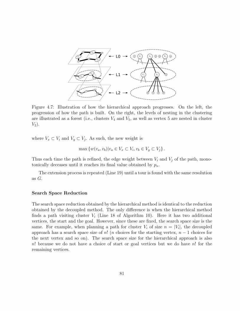
L0

L1

L2

Figure 4.7: Illustration of how the hierarchical approach progresses. On the left, theprogression of how the path is built. On the right, the levels of nesting in the clusteringare illustrated as a forest (i.e., clusters V4 and V5, as well as vertex 5 are nested in clusterV2).

where Vx ⊂ Vi and Vy ⊂ Vj. As such, the new weight is

max w(va, vb)|va ∈ Vx ⊂ Vi, vb ∈ Vy ⊂ Vj .

Thus each time the path is refined, the edge weight between Vi and Vj of the path, mono-tonically deceases until it reaches its final value obtained by pn.

The extension process is repeated (Line 19) until a tour is found with the same resolutionas G.

Search Space Reduction

The search space reduction obtained by the hierarchical method is identical to the reductionobtained by the decoupled method. The only difference is when the hierarchical methodfinds a path visiting cluster Vi (Line 18 of Algorithm 10). Here it has two additionalvertices, the start and the goal. However, since these are fixed, the search space size is thesame. For example, when planning a path for cluster Vi of size n = |Vi|, the decoupledapproach has a search space size of n! (n choices for the starting vertex, n− 1 choices forthe next vertex and so on). The search space size for the hierarchical approach is alson! because we do not have a choice of start or goal vertices but we do have n! for theremaining vertices.

81

Algorithm 10: Hierarchical-TSP(G,Γ)

Input:G: a graph with vertices V , edges E, and weights w.Γ: a real valued constant greater than 1.

Output:pn: a Hamiltonian tour G.

/* Find initial coarse solution */

1 C ← Find Γ-Clusters(G,Γ)2 C0 ← Roots(C)

3 G0 ← Coarsen(G,C0)

4 p0 ← ShortestTour(G0)/* Extend p0 to create p1 */

5 Vi ← p0[−1]6 p1 ← [] /* empty array */

7 for x ∈ 0, 1, . . . , |p0| − 1 do8 Vj ← p0[x]9 if Vj = p0[−1] then

10 Vk ← p1[0]

11 else12 Vk ← p0[x+ 1]

13 if |Vj| = 1 then14 Append Vj to p1

15 else16 CVj ← Vi ∪Children(Vj) ∪ Vk17 GVj ← Coarsen(G,CVj)

18 pVj ← ShortestPath(Vi, GVj , Vk)19 Append pVj to p1

20 Vi ← p1[−1]

21 Continue to extend p1, p2, . . . , pn until we have an array of unit clusters (vertices)22 return pn

82

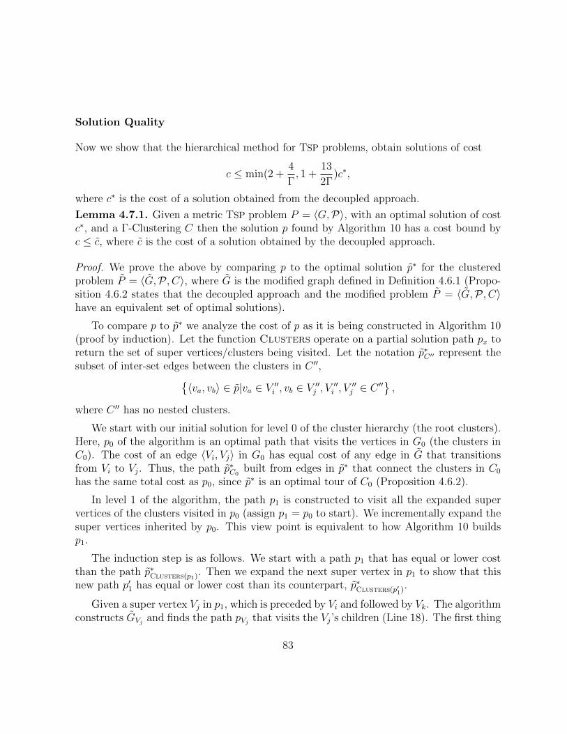
Solution Quality

Now we show that the hierarchical method for TSP problems, obtain solutions of cost

c ≤ min(2 +4

Γ, 1 +

13

2Γ)c∗,

where c∗ is the cost of a solution obtained from the decoupled approach.

Lemma 4.7.1. Given a metric TSP problem P = 〈G,P〉, with an optimal solution of costc∗, and a Γ-Clustering C then the solution p found by Algorithm 10 has a cost bound byc ≤ c, where c is the cost of a solution obtained by the decoupled approach.

Proof. We prove the above by comparing p to the optimal solution p∗ for the clusteredproblem P = 〈G,P , C〉, where G is the modified graph defined in Definition 4.6.1 (Propo-sition 4.6.2 states that the decoupled approach and the modified problem P = 〈G,P , C〉have an equivalent set of optimal solutions).

To compare p to p∗ we analyze the cost of p as it is being constructed in Algorithm 10(proof by induction). Let the function Clusters operate on a partial solution path px toreturn the set of super vertices/clusters being visited. Let the notation p∗C′′ represent thesubset of inter-set edges between the clusters in C ′′,

〈va, vb〉 ∈ p|va ∈ V ′′i , vb ∈ V ′′j , V ′′i , V ′′j ∈ C ′′,

where C ′′ has no nested clusters.

We start with our initial solution for level 0 of the cluster hierarchy (the root clusters).Here, p0 of the algorithm is an optimal path that visits the vertices in G0 (the clusters inC0). The cost of an edge 〈Vi, Vj〉 in G0 has equal cost of any edge in G that transitionsfrom Vi to Vj. Thus, the path p∗C0

built from edges in p∗ that connect the clusters in C0

has the same total cost as p0, since p∗ is an optimal tour of C0 (Proposition 4.6.2).

In level 1 of the algorithm, the path p1 is constructed to visit all the expanded supervertices of the clusters visited in p0 (assign p1 = p0 to start). We incrementally expand thesuper vertices inherited by p0. This view point is equivalent to how Algorithm 10 buildsp1.

The induction step is as follows. We start with a path p1 that has equal or lower costthan the path p∗Clusters(p1). Then we expand the next super vertex in p1 to show that thisnew path p′1 has equal or lower cost than its counterpart, p∗Clusters(p′1).

Given a super vertex Vj in p1, which is preceded by Vi and followed by Vk. The algorithmconstructs GVj and finds the path pVj that visits the Vj’s children (Line 18). The first thing

83

to note is that the incoming edges and outgoing edges for Vj in GVj are more accurate thanthey were before the expansion. They were w(Vi, Vj) = max w(va, vb)|va ∈ Vi, vb ∈ Vjand w(Vj, Vk) = max w(va, vb)|va ∈ Vj, vb ∈ Vk and now in GVj they have lesser or equalcost. For example, w(Vi, Vx) = max w(va, vb)|va ∈ Vi, vb ∈ Vx ⊂ Vj. If we were to usep∗CVj

as a candidate path for pVj then p1 after the expansion would have lesser or equal cost

to its counterpart. This is due to the cost of the path visiting Vj being equal in both cases.However, the incoming edges and outgoing edges have lesser or equal cost and the rest ofthe path has lesser or equal cost. Thus, Line 18 in the algorithm would choose pVj in sucha way to create p1 with equal or lower cost than the candidate path. Therefore, if we startwith a path p1 of equal or lower cost than its counter part p∗Clusters(p1) and expand it as inAlgorithm 10, the expanded path p′1 will have equal or lower cost than its counterpart.

This is the case when we start with p1 = p0. We repeat this step until all of theoriginal super vertices of p0 are expanded and then apply the same induction logic for eachsubsequent level until we get a path pn that can no longer be expanded with a solutioncost less than or equal to p∗. Therefore, c ≤ c.

Theorem 4.7.2 (Solution quality). Given a metric TSP problem P = 〈G,P〉, an optimalsolution of cost c∗, and a Γ-Clustering C, then the solution p found by Algorithm 10 hasa cost bound by

c ≤ min(2 +4

Γ, 1 +

13

2Γ)c∗.

Proof. The proof follows from Lemma 4.7.1 (the hierarchical approach finds solutions ofequal or lower cost than the decoupled approach) and Theorem 4.6.5 (the decoupled ap-proach finds solutions of cost c ≤ min(2 + 4

Γ, 1 + 13

2Γ)c∗).

4.7.2 A Hierarchical Method for Non-TSP Problems

The hierarchical approach builds a path by planning cluster Vi ∈ C semi-independentlyof the rest of the graph (it is semi-independent since it also considers the start and goalexternal to the cluster). This poses a challenge for solving non-TSP problems since theset of vertices included in the solution path is not known ahead of time. We provideAlgorithm 11 to solve this problem by extending Algorithm 10.

The extension (Algorithm 11) combines the decoupled approach with the hierarchicalapproach. The algorithm first determines the set of included vertices by solving the problemusing a decoupled approach (Line 2), then it finds a near optimal solution path using thehierarchical approach for TSP problems (Line 4).

84

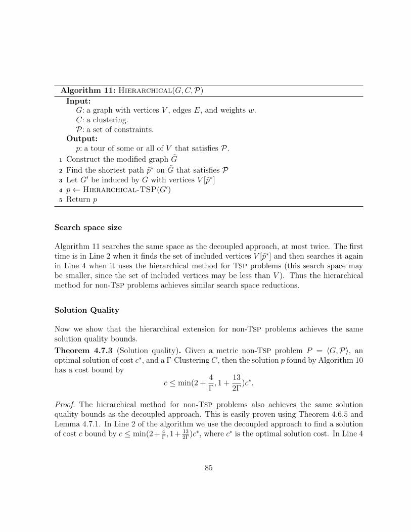
Algorithm 11: Hierarchical(G,C,P)

Input:G: a graph with vertices V , edges E, and weights w.C: a clustering.P : a set of constraints.

Output:p: a tour of some or all of V that satisfies P .

1 Construct the modified graph G

2 Find the shortest path p∗ on G that satisfies P3 Let G′ be induced by G with vertices V [p∗]4 p← Hierarchical-TSP(G′)5 Return p

Search space size

Algorithm 11 searches the same space as the decoupled approach, at most twice. The firsttime is in Line 2 when it finds the set of included vertices V [p∗] and then searches it againin Line 4 when it uses the hierarchical method for TSP problems (this search space maybe smaller, since the set of included vertices may be less than V ). Thus the hierarchicalmethod for non-TSP problems achieves similar search space reductions.

Solution Quality

Now we show that the hierarchical extension for non-TSP problems achieves the samesolution quality bounds.

Theorem 4.7.3 (Solution quality). Given a metric non-TSP problem P = 〈G,P〉, anoptimal solution of cost c∗, and a Γ-Clustering C, then the solution p found by Algorithm 10has a cost bound by

c ≤ min(2 +4

Γ, 1 +

13

2Γ)c∗.

Proof. The hierarchical method for non-TSP problems also achieves the same solutionquality bounds as the decoupled approach. This is easily proven using Theorem 4.6.5 andLemma 4.7.1. In Line 2 of the algorithm we use the decoupled approach to find a solutionof cost c bound by c ≤ min(2+ 4

Γ, 1+ 13

2Γ)c∗, where c∗ is the optimal solution cost. In Line 4

85

we improve the solution quality, thus preserves the cost bound. Therefore, Algorithm 11produces solutions with cost c bound by

c ≤ min(2 +4

Γ, 1 +

13

2Γ)c∗.

4.8 Experiments

This section presents the results of our experiments that demonstrate the effectiveness ofΓ-Clustering for solving discrete path planning problems. We benchmark the coupled plan-ning approach and the hierarchical planning approach against a non-clustered approach.All three methods use an ILP solver to find minimum length paths/tours. The benchmarkconsists of three different vehicle routing problems, TSP, sample collection, and periodrouting problems. The TSP instances are taken from TspLib [77], which provide a vari-ety of symmetric and non-symmetric environments. The sample collection and the periodrouting problems are taken from Section 3.6. They demonstrate the effectiveness of theproposed approaches on non-TSP problems. Additionally, we compare the quality of Γ-Clusters to clusters obtained by five other clustering approaches. In the rest of this section,we detail the generation of the sample collection and period routing problems followed byan analysis of the results.

4.8.1 Problem Library

Multi-Agent Sample Collection The setup of the sample collection problem is foundin Section 3.6.2 and the specifics are as follows. The robot’s environment is an obstacle freeEuclidean environment of size 1000×1000 meters. The instances contain 20 to 100 locationswhich are uniformly randomly distributed in the environment (easier instances have lesslocations). One location is randomly chosen to be the home location and the remaininglocations randomly contain either a small, medium, or large sample. The distribution ofthe samples are 3:1 for small to large and 2:1 for small to medium. The collection ofsamples in the environment contain 10-40 different minerals (easier problems have lessminerals). Each small sample has a mineral that is chosen uniformly randomly, similarlymedium samples have two minerals and large samples have three minerals chosen uniformlyrandomly (medium and large samples may choose the same mineral more than once). Thesmall robots have batteries that allow them to travel 3000 meters and the large robots

86

have batteries that allow them to travel 1500 meters. In Table 4.1 the naming convention#loc #mnr captures the number of locations and minerals of the problem.

Period Routing The setup of the period routing problem is found in Section 3.6.3,with the exception that back to back visits are allowed for the first and last periods.The specifics of the problem instances are as follows. The environment is an obstacle freeEuclidean environment of size 1000×1000 meters. The instances contain 25 to 35 locationswhich are uniformly randomly distributed in the environment (easier instances have lesslocations). One location is randomly chosen to be the home and the remaining locationsare customer locations. There are five service periods for which each customer may requireeither one, two, or three periods of service (uniformly and randomly assigned). In Table 4.1the naming convention #loc a captures the number of locations of the problem.

4.8.2 Setup and Execution

The Γ-Clustering algorithm was implemented in Python and run on an Intel Core i7-6700, 3.40GHz with 16GB of RAM. All Γ-Clustering experiments were conducted witha Γ = 1.000001, for which Theorem 4.5.11 implies that the coupled planning approachfinds solutions within min

(2, 1 + 3

2Γ

)-factor of the optimal. The hierarchical approach

finds solutions within min(2 + 4Γ, 1 + 13

2Γ)-factor of the optimal. However, the experiments

will show that the observed gap in performance is considerably closer to optimal than thebound. The ILP expression of the problem and clustered problem were solved on the samecomputer using Gurobi, also accessed through python.

The following is an ILP expression for TSP problems. We use this as a starting point

87

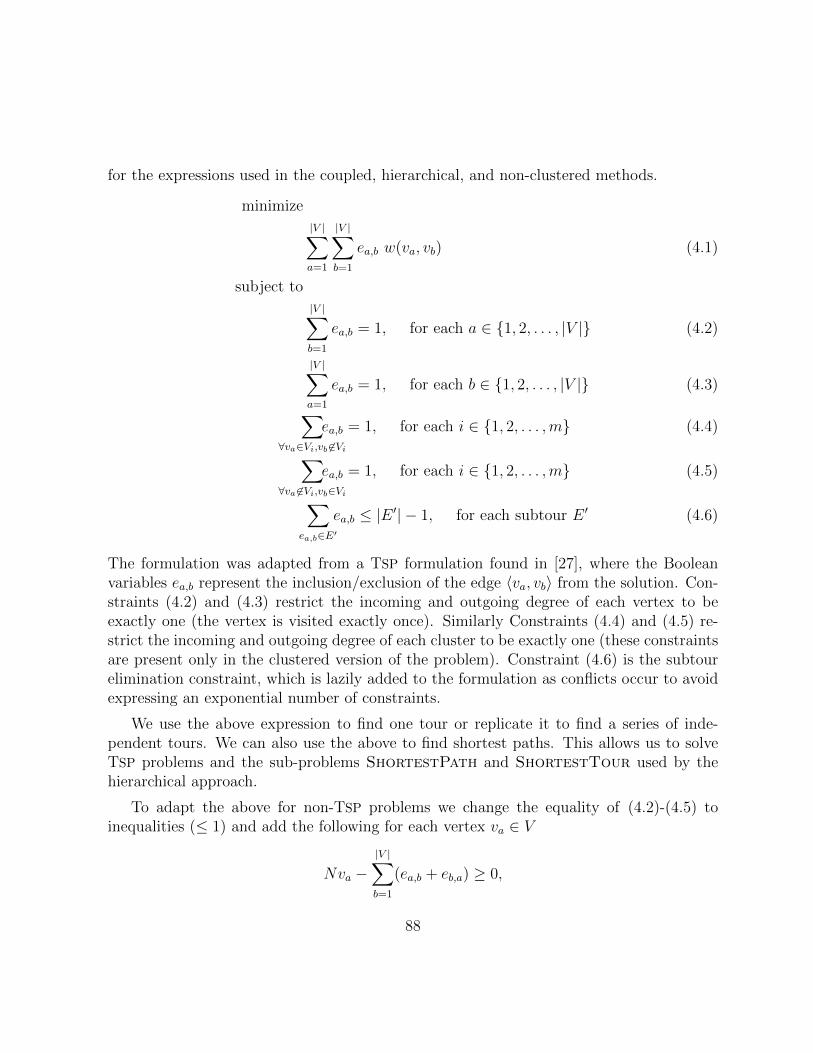
for the expressions used in the coupled, hierarchical, and non-clustered methods.

minimize

|V |∑a=1

|V |∑b=1

ea,b w(va, vb) (4.1)

subject to

|V |∑b=1

ea,b = 1, for each a ∈ 1, 2, . . . , |V | (4.2)

|V |∑a=1

ea,b = 1, for each b ∈ 1, 2, . . . , |V | (4.3)∑∀va∈Vi,vb 6∈Vi

ea,b = 1, for each i ∈ 1, 2, . . . ,m (4.4)∑∀va 6∈Vi,vb∈Vi

ea,b = 1, for each i ∈ 1, 2, . . . ,m (4.5)∑ea,b∈E′

ea,b ≤ |E ′| − 1, for each subtour E ′ (4.6)

The formulation was adapted from a TSP formulation found in [27], where the Booleanvariables ea,b represent the inclusion/exclusion of the edge 〈va, vb〉 from the solution. Con-straints (4.2) and (4.3) restrict the incoming and outgoing degree of each vertex to beexactly one (the vertex is visited exactly once). Similarly Constraints (4.4) and (4.5) re-strict the incoming and outgoing degree of each cluster to be exactly one (these constraintsare present only in the clustered version of the problem). Constraint (4.6) is the subtourelimination constraint, which is lazily added to the formulation as conflicts occur to avoidexpressing an exponential number of constraints.

We use the above expression to find one tour or replicate it to find a series of inde-pendent tours. We can also use the above to find shortest paths. This allows us to solveTSP problems and the sub-problems ShortestPath and ShortestTour used by thehierarchical approach.

To adapt the above for non-TSP problems we change the equality of (4.2)-(4.5) toinequalities (≤ 1) and add the following for each vertex va ∈ V

Nva −|V |∑b=1

(ea,b + eb,a) ≥ 0,

88

where N is some number bigger than |E|.We solve the shortest tour problem in Algorithm 11, Line 2 with the decoupled approach

by constructing a set of decoupled non-TSP problems and solving them as one instance.Recall from Section 4.6 that some additional logic is required to ensure that the decoupledapproach generates a solution tour instead of a path. This logic is required for the samplecollection and period routing problems. The construction of both of these problems containa home location that must be visited. We use the home location to create a hybrid cou-pled/decoupled problem, where the clusters that are not within the root cluster containingthe home vertex are solved with the decoupled approach and the clusters within the rootcluster that contain the home vertex are solved with the coupled approach. Clusters thatare solved with the decoupled approach that appear in the coupled problem, appear as asuper vertices.

The problem’s constraints P , also need to be encoded into the formulation. For exam-ple, the sample collection problem requires additional constraints to ensure each mineralin the environment is collected. Concretely, if location va and vb were the only locationsto contain mineral x then we would add the following to the formulation

|R|∑r=1

va,r + vb,r ≥ 1,

where va,r is the variable for robot r’s vertex location va and R is the set of robots. Similarly,to restrict back to back service for the period routing problem at location va, we add thefollowing constraint

va,p + vb,p+1 ≤ 1, for each p ∈ 1, 2, . . . , |P | − 1 ,

where va,p is the variable for the robot to visit location va on day p and P is the set ofdays.

4.8.3 Path planning with Γ-Clusters

In this section we benchmark the coupled approach and the hierarchical approach againsta non-clustered approach. The benchmark includes TSP, sample collection, and periodrouting problems. Each problem is solved three times and the average error and run timesare reported (run time includes time to find clusters as well as planing time). In the caseof the multi-agent sample collection problem and the periodic monitoring problem, theerror is measured from the best known solution (optimals are not known). Each problem

89

-0.01

0

0.01

0.02

0.03

0.04

0.05

0.06

Time01 Time02

Clu

ster

ing

Tim

e / T

otal

Tim

e

Figure 4.8: Box plot of the clustering time ratio with respect to the Γ-Clustering approach.The data is categorized by instances that did not time out (Time01) and instances thatdid time out (Time02).

is given a maximum time budget of 900 seconds to find the lowest cost solution tour. If thetime budget is reached before termination, the best solution up to that point is returned.The TSP instances shown in Table 4.2 are instances that have Γ-Clusters and are difficultenough so that the non-clustered approach took more than 30 seconds to solve but wasalso able to find solutions within 50% of optimal.

The first fact to note is that all three libraries have Γ-Clusters. Specifically, 63 outof 70 instances in the TspLib have Γ-Clusters and every sample collection and periodrouting problem contained Γ-Clusters. This shows that Γ-Clusters naturally occur in pathplanning problems since instances from the TspLib, along with the other two sets ofproblems represent a diverse collection of path planning environments. Overall there weremore than 3700 non-trivial Γ-Clusters (clusters of size two or more) in TspLib and 242non-trivial Γ-Clusters in the remaining instances. Additionally, the time spent finding Γ-Clusters was insignificant compared to the total time spent finding path planning solutions.Specifically, most instances spent less than 1% of their time finding clusters (all spent lessthan 6%). Although, the data is not explicitly presented in this chapter we noticed a trend,that as the instances became more difficult, the ratio of time spent finding Γ-Clusters tothe time spent finding solutions, shrank.

The results in Table 4.2 show how the two approaches improved the solver efficiency.Specifically, the non-clustered approach used 90% of their time budget compared to 73%and 41% for the coupled and hierarchical approaches, respectively. A few noteworthy ex-amples are gr96, bier127, and ch130. In all three examples the non-clustered approach tookmore than 20 times longer than the other two approaches. We see a similar improvement inefficiency for the coupled and hierarchical approaches. For example, the coupled approachtook more than 20 times longer for the instances kroB150, kroA200, and gr202.

90

0

10

20

30

40

50

60

Erro

r (%

)

No ClusteringGamma Clustering

Hierarchical

Instances (Easy Hard)

Figure 4.9: A plot of the average error for each solver method. Instances are sorted fromleast to most difficult.

The results show these approaches also achieve good solution quality. Specifically,all solutions obtained by these approaches were within 50% of optimal and most werewithin 5%. As a comparison, the non-clustered approach was able to solve 24 out of 44instances to within 5% of optimal while the coupled and hierarchical approaches were ableto respectively solve 32/44 and 42/44 instances to within 5% of optimal. Additionally, thereis a trend in the data, that as instances become more difficult to solve, the performance ofthe solvers degrade. However, we see from the data that the coupled approach degradesslower than the non-clustered approach and the hierarchical approach degrades at an evenslower rate than the other two approaches. This trend is shown more clearly in Figure 4.9,which plots the percent error verses the difficulty of the instance. As we can see fromthe figure, the hierarchical approach on average incurs a random error centred around 5%and that error does not degrade as the instances become more difficult. Thus, as instancesbecome more difficult to solve, we employ the coupled approach or the hierarchical approachto find better cost solutions.

Remark 4.8.1 (Using ILP solvers). It is worth emphasizing that although we use an ILPsolver to solve path planning problems, we are not recommending using ILP solvers ingeneral. For example, there are some very good TSP solvers that would greatly outperforma ILP solver for TSP instances. We are simply using ILP solvers to demonstrate how Γ-Clustering can be used to improve solver efficiency for path planning problems. Manydiscrete path planning problems are solved with ILP solvers and as such, we hope ourresults provide insight for how effective the proposed approaches are for path planningproblems.

91

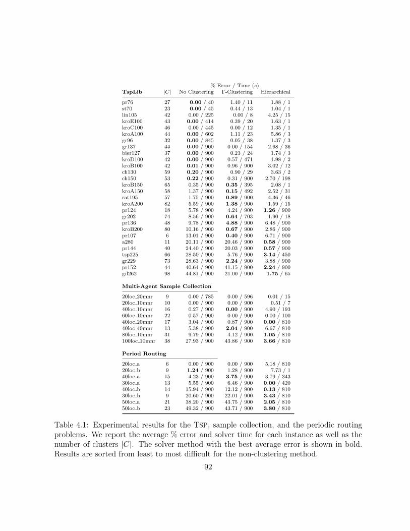
% Error / Time (s)TspLib |C| No Clustering Γ-Clustering Hierarchical

pr76 27 0.00 / 40 1.40 / 11 1.88 / 1st70 23 0.00 / 45 0.44 / 13 1.04 / 1lin105 42 0.00 / 225 0.00 / 8 4.25 / 15kroE100 43 0.00 / 414 0.39 / 20 1.63 / 1kroC100 46 0.00 / 445 0.00 / 12 1.35 / 1kroA100 44 0.00 / 602 1.11 / 23 5.86 / 3gr96 32 0.00 / 845 0.05 / 38 1.37 / 3gr137 44 0.00 / 900 0.00 / 154 2.68 / 36bier127 37 0.00 / 900 0.23 / 24 1.74 / 3kroD100 42 0.00 / 900 0.57 / 471 1.98 / 2kroB100 42 0.01 / 900 0.96 / 900 3.02 / 12ch130 59 0.20 / 900 0.90 / 29 3.63 / 2ch150 53 0.22 / 900 0.31 / 900 2.70 / 198kroB150 65 0.35 / 900 0.35 / 395 2.08 / 1kroA150 58 1.37 / 900 0.15 / 492 2.52 / 31rat195 57 1.75 / 900 0.89 / 900 4.36 / 46kroA200 82 5.59 / 900 1.38 / 900 1.59 / 15pr124 18 5.78 / 900 4.24 / 900 1.26 / 900gr202 74 8.56 / 900 0.64 / 703 1.90 / 18pr136 48 9.78 / 900 4.88 / 900 6.48 / 900kroB200 80 10.16 / 900 0.67 / 900 2.86 / 900pr107 6 13.01 / 900 0.40 / 900 6.71 / 900a280 11 20.11 / 900 20.46 / 900 0.58 / 900pr144 40 24.40 / 900 20.03 / 900 0.57 / 900tsp225 66 28.50 / 900 5.76 / 900 3.14 / 450gr229 73 28.63 / 900 2.24 / 900 3.88 / 900pr152 44 40.64 / 900 41.15 / 900 2.24 / 900gil262 98 44.81 / 900 21.00 / 900 1.75 / 65

Multi-Agent Sample Collection

20loc 20mnr 9 0.00 / 785 0.00 / 596 0.01 / 1520loc 10mnr 10 0.00 / 900 0.00 / 900 0.51 / 740loc 10mnr 16 0.27 / 900 0.00 / 900 4.90 / 19360loc 10mnr 22 0.57 / 900 0.00 / 900 0.00 / 10040loc 20mnr 17 3.04 / 900 0.87 / 900 0.00 / 81040loc 40mnr 13 5.38 / 900 2.04 / 900 6.67 / 81080loc 10mnr 31 9.79 / 900 4.12 / 900 1.05 / 810100loc 10mnr 38 27.93 / 900 43.86 / 900 3.66 / 810

Period Routing

20loc a 6 0.00 / 900 0.00 / 900 5.18 / 81020loc b 9 1.24 / 900 1.28 / 900 7.73 / 140loc a 15 4.23 / 900 3.75 / 900 3.79 / 34330loc a 13 5.55 / 900 6.46 / 900 0.00 / 42040loc b 14 15.94 / 900 12.12 / 900 0.13 / 81030loc b 9 20.60 / 900 22.01 / 900 3.43 / 81050loc a 21 38.20 / 900 43.75 / 900 2.05 / 81050loc b 23 49.32 / 900 43.71 / 900 3.80 / 810

Table 4.1: Experimental results for the TSP, sample collection, and the periodic routingproblems. We report the average % error and solver time for each instance as well as thenumber of clusters |C|. The solver method with the best average error is shown in bold.Results are sorted from least to most difficult for the non-clustering method.

92

4.8.4 Other Clustering Methods

In this section we compare the quality of Γ-Clusters to the quality of clusters obtained byother methods.

The ideal test of a clustering’s quality for path planning is a measure of how much theoptimal path(s) degrade in quality when the clustered problem is solved (Problem 4.3.3solved with the coupled approach) instead of the non-clustered problem (Problem 4.3.2).Solving these problems (finding an optimal) may require large amounts of time and so weopted to make this comparison on TSP problem instances since they are easier to solvethan non-TSP problems. Additionally, the TSP problem instances we solve cover a diverseset of environments, thus giving us a good basis for comparison.

We compare the Γ-Clustering method to a set of community structure methods from theiGraph library [16]. Specifically, we tested against a fast greedy approach [14], Newman’sleading eigenvector method [61], a multilevel algorithm [8], spinglass [76], and walktrap [72].

The objective of community structures is to find clusters that are intimately connectedin a sparse network (a multigraph). The connections (edges) usually represent a relation-ship or common trait between the nodes, such as a friendship in a social network. Eachconnection is represented with an edge; more edges mean more shared traits.

To utilize community structures for path planning (find clusters of locations that arein close proximity) we transform the problem graph into a network by “inverting” theweighted graph into a unweighted multigraph (network). Specifically, we translate an edgevi,j with weight w(i, j) in the problem graph to maxj,k w(j, k)−w(i, j) edges in the network.The nodes in the new network, are highly connected, if they were in close proximity in theoriginal graph. Thus the obtained community structures in the network resemble the typeof clusters we study in this chapter.

The goodness of a community structure is often measured with a metric called modular-ity [62] (not necessarily the same metric for each algorithm), meaning that many commu-nity methods work towards the same goal. However, since the task of finding the optimalclustering is NP-hard, the different algorithms often produce different results.

Some of the methods in the iGraph library provide metadata that gives insight into theoptimal number of clusters and how the clusters were built. We used this information andthe threshold modularity parameter to produce clusterings of a similar size to those foundby the Γ-Clustering approach.

The results of the experiments are given in Table 4.2. They show that the quality ofthe Γ-Clusterings often outperform the quality of the clusterings found by other methods.

93

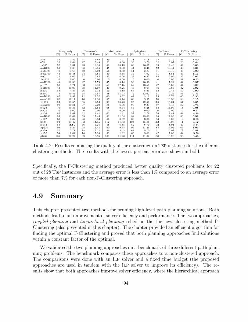
Fastgreedy Newman’s Multilevel Spinglass Walktrap Γ-Clustering|C| % Error |C| % Error |C| % Error |C| % Error |C| % Error |C| % Error

pr76 32 7.86 27 11.69 29 7.41 38 8.18 43 6.16 27 1.40st70 32 8.44 27 5.48 23 4.00 30 3.70 32 6.07 23 0.44lin105 52 9.31 43 19.15 52 16.13 60 16.67 39 12.46 42 0.00kroE100 35 8.68 38 10.15 45 9.30 47 8.46 52 13.44 43 0.39kroC100 40 3.68 42 13.93 56 2.82 51 3.87 51 13.15 46 0.00kroA100 48 15.38 44 7.81 39 8.35 37 4.92 41 8.81 44 1.11gr96 25 6.06 27 6.85 25 6.06 27 6.47 14 2.96 32 0.05bier127 0 0.00 0 0.00 0 0.00 0 0.00 0 0.00 37 0.23kroD100 48 12.56 47 17.79 45 8.14 53 10.90 41 7.29 42 0.57gr137 30 9.71 63 19.10 51 17.15 52 13.51 47 15.63 44 0.00kroB100 43 10.03 38 11.07 40 9.25 43 8.64 46 9.66 42 0.92ch130 58 4.44 56 12.14 59 4.12 64 8.25 63 9.44 59 0.90ch150 75 10.55 68 17.57 58 11.03 72 12.62 51 9.24 53 0.31kroB150 67 6.89 72 9.57 60 3.57 67 3.11 75 15.76 65 0.35kroA150 62 11.17 70 11.10 57 8.74 63 9.95 78 10.36 58 0.15rat195 93 18.55 105 19.54 91 16.23 95 19.50 116 16.01 57 0.65kroA200 99 10.81 97 12.29 86 6.66 90 9.37 87 8.48 82 0.73pr124 70 10.36 52 11.64 68 9.44 55 8.28 63 11.99 18 0.08gr202 0 0.00 0 0.00 0 0.00 0 0.00 0 0.00 74 0.57pr136 62 1.41 62 1.41 62 1.41 57 2.78 58 1.41 48 4.88kroB200 95 12.62 103 17.45 81 11.04 84 13.08 95 11.96 80 0.52pr107 60 0.62 68 0.84 60 0.62 66 3.00 34 0.00 6 0.00a280 94 13.42 133 14.35 112 11.63 104 15.86 113 19.00 11 0.12pr144 58 2.89 66 5.25 58 6.85 82 6.79 72 8.91 40 3.34tsp225 99 9.24 108 11.41 90 9.35 94 11.26 85 15.02 66 1.05gr229 37 2.71 78 12.21 36 3.53 67 5.70 51 15.03 73 0.88pr152 54 1.02 74 7.39 53 1.02 66 3.08 47 7.06 44 3.76gil262 126 12.24 109 13.75 101 11.23 111 11.02 130 10.98 98 0.46

Table 4.2: Results comparing the quality of the clusterings on TSP instances for the differentclustering methods. The results with the lowest percent error are shown in bold.

Specifically, the Γ-Clustering method produced better quality clustered problems for 22out of 28 TSP instances and the average error is less than 1% compared to an average errorof more than 7% for each non-Γ-Clustering approach.

4.9 Summary

This chapter presented two methods for pruning high-level path planning solutions. Bothmethods lead to an improvement of solver efficiency and performance. The two approaches,coupled planning and hierarchical planning relied on the the new clustering method Γ-Clustering (also presented in this chapter). The chapter provided an efficient algorithm forfinding the optimal Γ-Clustering and proved that both planning approaches find solutionswithin a constant factor of the optimal.

We validated the two planning approaches on a benchmark of three different path plan-ning problems. The benchmark compares these approaches to a non-clustered approach.The comparisons were done with an ILP solver and a fixed time budget (the proposedapproaches are used in tandem with the ILP solver to improve its efficiency). The re-sults show that both approaches improve solver efficiency, where the hierarchical approach

94

achieves more time savings than the coupled approach but poorer solution quality for in-stances solved within the time budget. Both approaches found solutions much closer tooptimal than their quality bounds — most solutions were within 10% of optimal. For themore difficult instances the results showed that these approaches maintained their perfor-mance longer than the non-clustered approach (the hierarchical approach maintained itsperformance longer than the coupled approach). Thus these approaches can be used tofind higher quality solutions than the non-clustered approach for more difficult instances.Additionally, this chapter compared the quality of Γ-Clusterings to clusterings found byfive other methods. The results showed that Γ-Clusterings provided the highest qualitysolutions for use in path planning.

95

Chapter 5

Conclusions

This thesis concentrated on solving high-level path planning problems. We started outlearning how to solve high-level path planning problems with an ILP approach and thenlearned about an alternative approach called SAT-TSP in Chapter 3. This approach usedthe problem language SAT-TSP to model high-level path planning problems. The problemitself is a combination of two well known problems, SAT and TSP. The structure of thisproblem allowed us to leverage the SMT framework to combine state-of-the-art SAT andTSP solvers together to create the CBTSP solver. We used this solver to find solutions fora variety of path planning problems and the results showed that the CBTSP solver oftenoutperformed a commercial ILP solver. Thus making CBTSP a good candidate for solvinghigh-level path planning problems. The CBTSP solver is available at https://github.

com/fcimeson/cbTSP.

In Chapter 4, we explored two approaches for pruning high-level path planning solutionsand thus improving solver efficiency. The first approach, coupled planning, achieves itsperformance gains by trading off solution quality. The trade however, is not a drastic. Weproved in this chapter that solutions found by this approach are within a constant factorof min

(2, 1 + 3

2Γ

)of the optimal. The second approach, hierarchical planning, provides a

more aggressive method to achieve even more performance gains while still finding solutionswithin a constant factor of min(2 + 4

Γ, 1 + 13

2Γ) of the optimal. We tested these approaches

with an ILP solver on a series of path planning problems. The results showed that, notonly are these approaches more efficient than a non-clustered approach, they can also beused to find higher quality solutions when solver time is limited.

Both of these approaches rely on a new clustering method introduced in this chaptercalled Γ-Clustering. We provided an efficient method for find the optimal Γ-Clustering.

96



We compared the quality of Γ-Clusterings to clusterings found by other methods, to showthat Γ-Clusterings are more useful for path planning problems.

5.1 Future Work

5.1.1 SAT-TSP

Below we provide a list of the areas of future work for related to SAT-TSP.

A Modelling Language We do not expect that every user will be willing to modeltheir problem as a SAT-TSP expression. As such we are in the process of developing amodelling language for SAT-TSP. This language will allow the user to express/model theirproblem in a more user-friendly format. The format will preserve the important structuresour software needs so that it can translate the model to SAT-TSP. Additionally, the useof a modelling language will allow the user to separate the problem definition from theproblem instance. For example, one would be able to express the TSP problem as a modeland then separately express the problem instance as a transition environment (a graph).This benefits the user in two ways: readability and repeatability. The problem model ismore readable because the large environmental data is not cluttering the problem definitionand the problem model can be reused to prevent user error in re-specifying the problem,making it more repeatable.

Search Heuristics We are working on improving the CBTSP solver, specifically, CBTSP’ssearch heuristics. Currently CBTSP uses the DPLL search heuristic for choosing the orderof variable assignments. We believe incorporating knowledge of the TSP problem into theheuristics would improve the solvers performance.

Other SMT Theories Another area of development, is to expand upon the CBTSP

solver by incorporating more SMT theories (currently CBTSP only uses one theory, theTSP theory). In this way we could natively handle more path planning constraints such asordering constraints.

SMT Propagation We can further improve the CBTSP solver by incorporating SMT

propagation. Currently the only SMT technique CBTSP uses clause negations. If we were

97

to incorporate into the SMT theories some knowledge of the problem structure, such asset cardinality constraints and/or ordering constraints. We could use those theories topropagate variable assignments to the SAT solver instead of encoding those constraints asSAT formulae. Briefly consider the “exactly one-in-a-set” cardinality constraint for the setS as an example. In this case, if the SAT solver chose one of the literals in S to be true,then the theory would propagate the knowledge that all other literals in the set must befalse. This example reduces the size of the SAT formula by |S|2 which we expect wouldimprove the solver’s efficiency.

Collisions We plan to investigate the effectiveness of using SAT-TSP for collision avoid-ance problems. Our approach would extend the environment graph to incorporate dis-cretized time steps. In this way, we can use the location/time vertices to prohibit multiplerobots from occupying the same location during the same discrete time step as in [102].

Parallelization We are looking into upgrading CBTSP to utilize multiple threads. Toaccomplish this we would implement a multi-threaded SAT solver, which in turn wouldmake threaded calls to a TSP solver.

5.1.2 Γ-Clustering

The areas of future work for using Γ-Clusterings to improve solver efficiency are as follows.

Improve Solution Quality Bounds We are currently working towards improving thetightness of the solution quality bounds presented in Theorems 4.5.11, 4.7.2, and 4.7.3.Additionally, we are trying to find problem instances that better characterize the tightnessof these bounds.

Parallelization We plan on developing new algorithms that use parallel processes tofind high quality solution paths for discrete path planning problems. The decoupled andhierarchical planning approach is setup to work with parallelization (decoupled more thanhierarchical). To parallelize the hierarchical approach we can change how the algorithmexpands the super vertices in the coarsened tour. Specifically, we could use parallel pro-cesses to expand every other super vertex in the tour. Then, after those processes are donewe would again use parallel processes to expand the remaining super vertices.

98

Dynamic Planning We are currently working on techniques based on Γ-Clusterings fordynamic planning. Here Γ-Clusters are used to decompose an existing solution path intoregions that may be preserved and regions that need to be replanned. Then the hierarchicalapproach is used to fill in the missing regions of the path and find solutions that are withina constant factor of the optimal.

Applications Finally, we plan to search for more applications that may benefit fromthe Γ-Clustering approaches presented in this thesis. Specifically, we are looking to findcommon solver approaches that can be improved by the proposed approaches.

99

References

[1] IBM ILOG CPLEX Optimizer, 2010.

[2] Tobias Achterberg. SCIP: solving constraint integer programs. Mathematical Pro-gramming Computation, 1(1):1–41, 2009.

[3] David Applegate, Robert Bixby, Vasek Chvatal, and William Cook. Concorde TSPsolver. Accessed: 2015-03-05.

[4] David L Applegate, Robert E Bixby, Vasek Chvatal, and William J Cook. TheTraveling Salesman Problem: A Computational Study. Princeton University Press,2006.

[5] Sanjeev Arora. Polynomial time approximation schemes for euclidean traveling sales-man and other geometric problems. Journal of the ACM (JACM), 45(5):753–782,1998.

[6] Luca Bertazzi and M Grazia Speranza. Inventory routing problems with multiplecustomers. EURO Journal on Transportation and Logistics, 2(3):255–275, 2013.

[7] Graeme Best, Jan Faigl, and Robert Fitch. Multi-robot path planning for budgetedactive perception with self-organising maps. In IEEE/RSJ International Conferenceon Intelligent Robots and Systems, pages 3164–3171, 2016.

[8] Vincent D Blondel, Jean-Loup Guillaume, Renaud Lambiotte, and Etienne Lefebvre.Fast unfolding of communities in large networks. Journal of statistical mechanics:theory and experiment, 2008(10):P10008, 2008.

[9] Stanislav Bochkarev and Stephen L Smith. On minimizing turns in robot cover-age path planning. In IEEE International Conference on Automation Science andEngineering (CASE), pages 1237–1242, 2016.

100

[10] Howie Choset. Coverage for robotics–a survey of recent results. Annals of Mathe-matics and Artificial Intelligence, 31(1-4):113–126, 2001.

[11] Nicos Christofides and John E Beasley. The period routing problem. Networks,14(2):237–256, 1984.

[12] Alessandro Cimatti, Edmund Clarke, Enrico Giunchiglia, Fausto Giunchiglia, MarcoPistore, Marco Roveri, Roberto Sebastiani, and Armando Tacchella. NuSMV 2: Anopensource tool for symbolic model checking. In Computer Aided Verification, pages359–364. Springer, 2002.

[13] Jens Clausen. Branch and bound algorithms-principles and examples. Departmentof Computer Science, University of Copenhagen, pages 1–30, 1999.

[14] Aaron Clauset, Mark EJ Newman, and Cristopher Moore. Finding community struc-ture in very large networks. Physical Review E, 70(6):066111, 2004.

[15] Leandro C Coelho and Gilbert Laporte. The exact solution of several classes ofinventory-routing problems. Computers & Operations Research, 40(2):558–565, 2013.

[16] Gabor Csardi and Tamas Nepusz. The igraph software package for complex networkresearch. InterJournal: Complex Systems, page 1695, 2006.

[17] Arun Das, Michael Diu, Neil Mathew, Christian Scharfenberger, James Servos, AndyWong, John S Zelek, David A Clausi, and Steven L Waslander. Mapping, plan-ning, and sample detection strategies for autonomous exploration. Journal of FieldRobotics, 31(1):75–106, 2014.

[18] Martin Davis, George Logemann, and Donald Loveland. A machine program fortheorem-proving. Communications of the ACM, 5(7):394–397, 1962.

[19] Martin Davis and Hilary Putnam. A computing procedure for quantification theory.Journal of the ACM, 7(3):201–215, 1960.

[20] Markus Eich, Ronny Hartanto, Sebastian Kasperski, Sankaranarayanan Natarajan,and Johannes Wollenberg. Towards coordinated multirobot missions for lunar samplecollection in an unknown environment. Journal of Field Robotics, 31(1):35–74, 2014.

[21] Kutluhan Erol, Dana S Nau, and Venkatramana S Subrahmanian. Complexity, de-cidability and undecidability results for domain-independent planning. Artificial in-telligence, 76(1):75–88, 1995.

101

[22] Abdulah Fajar, Nur Azman Abu, and Nanna Suryana Herman. Clustering strategyto Euclidean TSP Hamilton path role in tour construction. In IEEE InternationalConference on Computer Modeling and Simulation, volume 3, pages 508–512, 2010.

[23] Dave Ferguson and Anthony Stentz. Using interpolation to improve path planning:The field D* algorithm. Journal of Field Robotics, 23(2):79–101, 2006.

[24] Richard E Fikes and Nils J Nilsson. STRIPS: A new approach to the application oftheorem proving to problem solving. Artificial intelligence, 2(3-4):189–208, 1971.

[25] Maria Fox and Derek Long. PDDL2.1: An extension to PDDL for expressing tem-poral planning domains. Journal of Artificial Intelligence Research, 20:61–124, 2003.

[26] Marc J Gallant, Alex Ellery, and Joshua A Marshall. Rover-based autonomousscience by probabilistic identification and evaluation. Journal of Intelligent & RoboticSystems, 72(3-4):591–613, 2013.

[27] Luis Gouveia and Jose Manuel Pires. The asymmetric travelling salesman problemand a reformulation of the miller–tucker–zemlin constraints. European Journal ofOperational Research, 112(1):134–146, 1999.

[28] Sudipto Guha, Rajeev Rastogi, and Kyuseok Shim. CURE: an efficient clusteringalgorithm for large databases. In ACM SIGMOD Record, volume 27, pages 73–84,1998.

[29] Sudipto Guha, Rajeev Rastogi, and Kyuseok Shim. ROCK: A robust clustering al-gorithm for categorical attributes. In International Conference on Data Engineering,pages 512–521, 1999.

[30] Gregory Gutin and Daniel Karapetyan. A memetic algorithm for the generalizedtraveling salesman problem. Natural Computing, 9(1):47–60, 2010.

[31] Yll Haxhimusa, Walter G Kropatsch, Zygmunt Pizlo, and Adrian Ion. Approximativegraph pyramid solution of the E-TSP. Image and Vision Computing, 27(7):887–896,2009.

[32] Keld Helsgaun. An effective implementation of the Lin–Kernighan traveling salesmanheuristic. European Journal of Operational Research, 126(1):106–130, 2000.

[33] Keld Helsgaun. Solving the equality generalized traveling salesman problem usingthe Lin–Kernighan–Helsgaun Algorithm. Mathematical Programming Computation,7:1–19, 2014.

102

[34] Jorg Hoffmann and Bernhard Nebel. The FF planning system: Fast plan generationthrough heuristic search. Journal of Artificial Intelligence Research, pages 253–302,2001.

[35] Geoffrey A Hollinger and Gaurav S Sukhatme. Sampling-based robotic informationgathering algorithms. The International Journal of Robotics Research, 33(9):1271–1287, 2014.

[36] Gerard J Holzmann. The SPIN model checker: Primer and reference manual, volume1003. Addison-Wesley, 2004.

[37] Holger H Hoos and Thomas Stutzle. SATLIB–the satisfiability library, 1998.

[38] William NN Hung, Xiaoyu Song, Jindong Tan, Xiaojuan Li, Jie Zhang, Rui Wang,and Peng Gao. Motion planning with satisfiability modulo theories. In IEEE Inter-national Conference on Robotics and Automation (ICRA), pages 113–118, 2014.

[39] Frank Imeson and Stephen L Smith. A language for robot path planning in discreteenvironments: The TSP with Boolean satisfiability constraints. In IEEE Interna-tional Conference on Robotics and Automation (ICRA), pages 5772–5777, 2014.

[40] Frank Imeson and Stephen L Smith. Multi-robot task planning and sequencingusing the SAT-TSP language. In IEEE International Conference on Robotics andAutomation (ICRA), pages 5397–5402, 2015.

[41] Paul Jackson and Davisniel Sheridan. Clause form conversions for Boolean circuits.In Theory and Applications of Satisfiability Testing, pages 183–198. Springer, 2005.

[42] Anil K Jain. Data clustering: 50 years beyond k-means. Pattern Recognition Letters,31(8):651–666, 2010.

[43] Subbarao Kambhampati and Larry Davis. Multiresolution path planning for mobilerobots. IEEE Journal on Robotics and Automation, 2(3):135–145, 1986.

[44] Nitin Kamra and Nora Ayanian. A mixed integer programming model for timeddeliveries in multirobot systems. In IEEE International Conference on AutomationScience and Engineering (CASE), pages 612–617, 2015.

[45] George Karypis and Vipin Kumar. A fast and high quality multilevel scheme forpartitioning irregular graphs. SIAM Journal on Scientific Computing, 20(1):359–392, 1998.

103

[46] Brian W Kernighan and Shen Lin. An efficient heuristic procedure for partitioninggraphs. Bell System Technical Journal, 49(2):291–307, 1970.

[47] Jon Kleinberg and Eva Tardos. Algorithm Design. Addison-Wesley, 2006.

[48] Marius Kloetzer and Calin Belta. Automatic deployment of distributed teams ofrobots from temporal logic motion specifications. IEEE Transactions on Robotics,26(1):48–61, 2010.

[49] Bernhard Korte, Jens Vygen, B Korte, and J Vygen. Combinatorial Optimization,volume 2. Springer, 2012.

[50] James Kuffner, Koichi Nishiwaki, Satoshi Kagami, Masayuki Inaba, and HirochikaInoue. Motion planning for humanoid robots. Robotics Research, pages 365–374,2005.

[51] Ailsa H Land and Alison G Doig. An automatic method of solving discrete program-ming problems. Econometrica: Journal of the Econometric Society, pages 497–520,1960.

[52] Steven Michael LaValle. Planning Algorithms. Cambridge University Press, 2006.

[53] Maxim Likhachev and Dave Ferguson. Planning long dynamically feasible maneuversfor autonomous vehicles. The International Journal of Robotics Research, 28(8):933–945, 2009.

[54] S. Lin and B. W. Kernighan. An effective heuristic algorithm for the traveling-salesman problem. Operations Research, 21:498–516, 1973.

[55] M. Morris Mano and Michael D. Ciletti. Digital Design. Prentice-Hall, Inc., 4 edition,2006.

[56] Neil Mathew, Stephen L Smith, and Steven Lake Waslander. Multirobot ren-dezvous planning for recharging in persistent tasks. IEEE Transactions on Robotics,31(1):128–142, 2015.

[57] Clair E Miller, Albert W Tucker, and Richard A Zemlin. Integer programmingformulation of traveling salesman problems. Journal of the ACM (JACM), 7(4):326–329, 1960.

104

[58] Joseph SB Mitchell. Guillotine subdivisions approximate polygonal subdivisions:A simple polynomial-time approximation scheme for geometric TSP, k-MST, andrelated problems. SIAM Journal on Computing, 28(4):1298–1309, 1999.

[59] Matthew W Moskewicz, Conor F Madigan, Ying Zhao, Lintao Zhang, and SharadMalik. Chaff: Engineering an efficient sat solver. In Proceedings of the 38th annualDesign Automation Conference, pages 530–535. ACM, 2001.

[60] Srinivas Nedunuri, Sailesh Prabhu, Mark Moll, Swarat Chaudhuri, and Lydia EKavraki. SMT-based synthesis of integrated task and motion plans from plan out-lines. In IEEE International Conference on Robotics and Automation (ICRA), pages655–662, 2014.

[61] Mark EJ Newman. Finding community structure in networks using the eigenvectorsof matrices. Physical Review E, 74(3):036104, 2006.

[62] Mark EJ Newman and Michelle Girvan. Finding and evaluating community structurein networks. Physical Review E, 69(2):026113, 2004.

[63] Robert Nieuwenhuis, Albert Oliveras, and Cesare Tinelli. Solving SAT and SATmodulo theories: From an abstract Davis–Putnam–Logemann–Loveland procedureto DPLL(T). Journal of the ACM, 53(6):937–977, 2006.

[64] Karl J Obermeyer, Paul Oberlin, and Swaroop Darbha. Sampling-based roadmapmethods for a visual reconnaissance UAV. In AIAA Conference on Guidance, Navi-gation and Control, 2010.

[65] Karl J Obermeyer, Paul Oberlin, and Swaroop Darbha. Sampling-based path plan-ning for a visual reconnaissance unmanned air vehicle. Journal of Guidance, Control,and Dynamics, 35(2):619–631, 2012.

[66] Gurobi Optimization et al. Gurobi optimizer reference manual, 2012.

[67] Christos H Papadimitriou and Kenneth Steiglitz. Combinatorial Optimization: Al-gorithms and Complexity. Dover Publications, 1998.

[68] Junghee Park, Sisir Karumanchi, and Karl Iagnemma. Homotopy-based divide-and-conquer strategy for optimal trajectory planning via mixed-integer programming.IEEE Transactions on Robotics, 31(5):1101–1115, 2015.

[69] Gabor Pataki. The bad and the good-and-ugly: formulations for the traveling sales-man problem, 2000.

105

[70] Gabor Pataki. Teaching integer programming formulations using the traveling sales-man problem. SIAM review, 45(1):116–123, 2003.

[71] Sandro Pirkwieser and Gunther R Raidl. Multilevel variable neighborhood searchfor periodic routing problems. In EvoCOP, pages 226–238. Springer, 2010.

[72] Pascal Pons and Matthieu Latapy. Computing communities in large networks usingrandom walks. In ISCIS, volume 3733, pages 284–293, 2005.

[73] David Portugal and Rui P Rocha. Cooperative multi-robot patrol with bayesianlearning. Autonomous Robots, 40(5):929–953, 2016.

[74] Robert Clay Prim. Shortest connection networks and some generalizations. BellSystem Technical Journal, 36(6):1389–1401, 1957.

[75] Morgan Quigley, Ken Conley, Brian Gerkey, Josh Faust, Tully Foote, Jeremy Leibs,Rob Wheeler, and Andrew Y Ng. ROS: an open-source robot operating system. InICRA Workshop on Open Source Software, volume 3.2, page 5, 2009.

[76] Jorg Reichardt and Stefan Bornholdt. Statistical mechanics of community detection.Physical Review E, 74(1):016110, 2006.

[77] Gerhard Reinelt. TSPLIB–a traveling salesman problem library. ORSA Journal onComputing, 3(4):376–384, 1991.

[78] Silvia Richter and Matthias Westphal. The LAMA planner: Guiding cost-based any-time planning with landmarks. Journal of Artificial Intelligence Research, 39(1):127–177, 2010.

[79] Demane Rodney, Alan Soper, and Chris Walshaw. The application of multilevelrefinement to the vehicle routing problem. In IEEE Symposium on ComputationalIntelligence in Scheduling (SCIS), pages 212–219, 2007.

[80] Indranil Saha, Rattanachai Ramaithitima, Vijay Kumar, George J Pappas, and San-jit A Seshia. Automated composition of motion primitives for multi-robot systemsfrom safe LTL specifications. In IEEE/RSJ International Conference on IntelligentRobots and Systems, pages 1525–1532, 2014.

[81] Mitul Saha, Tim Roughgarden, Jean-Claude Latombe, and Gildardo Sanchez-Ante.Planning tours of robotic arms among partitioned goals. The International Journalof Robotics Research, 25(3):207–223, 2006.

106

[82] Peter Sanders and Dominik Schultes. Highway hierarchies hasten exact shortest pathqueries. In European Symposium on Algorithms, pages 568–579. Springer, 2005.

[83] Satu Elisa Schaeffer. Graph clustering. Computer Science Review, 1(1):27–64, 2007.

[84] Peter Schuller, Volkan Patoglu, and Esra Erdem. A systematic analysis of levels ofintegration between low-level reasoning and task planning. In Workshop on Com-bining Task and Motion Planning (IEEE International Conference on Robotics andAutomation), 2013.

[85] Christian Schulte, Guido Tack, and Mikael Z Lagerkvist. Modeling and programmingwith Gecode, 2010.

[86] Yasser Shoukry, Pierluigi Nuzzo, Indranil Saha, Alberto L Sangiovanni-Vincentelli,Sanjit A Seshia, George J Pappas, and Paulo Tabuada. Scalable lazy SMT-basedmotion planning. In 55th Conference on Decision and Control (CDC), pages 6683–6688. IEEE, 2016.

[87] A Prasad Sistla and Edmund M Clarke. The complexity of propositional lineartemporal logics. Journal of the ACM, 32(3):733–749, 1985.

[88] Stephen L Smith and Frank Imeson. GLNS: An effective large neighborhood searchheuristic for the generalized traveling salesman problem. Computers & OperationsResearch, 2017.

[89] Stephen L Smith, Jana Tumova, Calin Belta, and Daniela Rus. Optimal path plan-ning for surveillance with temporal-logic constraints. The International Journal ofRobotics Research, 30(14):1695–1708, 2011.

[90] Niklas Sorensson and Niklas Een. MiniSat v1.13 – a SAT solver with conflict-clauseminimization. SAT, 2005:53, 2005.

[91] Ioan Alexandru Sucan, Mark Moll, and Lydia E Kavraki. The open motion planninglibrary. IEEE Robotics & Automation Magazine, 19(4):72–82, 2012.

[92] Yuichi Tazaki and Takumi Suzuki. Constraint-based prioritized trajectory planningfor multibody systems. IEEE Transactions on Robotics, 30(5):1227–1234, 2014.

[93] Pratap Tokekar, Joshua Vander Hook, David Mulla, and Volkan Isler. Sensor plan-ning for a symbiotic UAV and UGV system for precision agriculture. IEEE Trans-actions on Robotics, 32(6):1498–1511, 2016.

107

[94] Paolo Toth and Daniele Vigo. Vehicle routing: problems, methods, and applications.SIAM, 2014.

[95] Mauro Vallati, Lukas Chrpa, Marek Grzes, Thomas L McCluskey, Mark Roberts, andScott Sanner. The 2014 international planning competition: Progress and trends. AIMagazine, 36(3):90–98, 2015.

[96] Toby Walsh. SAT vs CSP. In Principles and Practice of Constraint Programming,pages 441–456. Springer, 2000.

[97] Chris Walshaw. A multilevel approach to the travelling salesman problem. OperationsResearch, 50(5):862–877, 2002.

[98] Richard Wang, Manuela Veloso, and Srinivasan Seshan. Active sensing data collectionwith autonomous mobile robots. In IEEE International Conference on Robotics andAutomation (ICRA), pages 2583–2588, 2016.

[99] Christopher Xie, Jur van den Berg, Sachin Patil, and Pieter Abbeel. Toward asymp-totically optimal motion planning for kinodynamic systems using a two-point bound-ary value problem solver. In IEEE International Conference on Robotics and Au-tomation (ICRA), pages 4187–4194, 2015.

[100] Baozhen Yao, Ping Hu, Mingheng Zhang, and Shuang Wang. Artificial bee colony al-gorithm with scanning strategy for the periodic vehicle routing problem. Simulation,89(6):762–770, 2013.

[101] Jingjin Yu, Sertac Karaman, and Daniela Rus. Persistent monitoring of events withstochastic arrivals at multiple stations. IEEE Transactions on Robotics, 31(3):521–535, 2015.

[102] Jingjin Yu and Steven M LaValle. Optimal multirobot path planning on graphs:Complete algorithms and effective heuristics. IEEE Transactions on Robotics,32(5):1163–1177, 2016.

[103] Tian Zhang, Raghu Ramakrishnan, and Miron Livny. BIRCH: an efficient dataclustering method for very large databases. In ACM Sigmod Record, volume 25,pages 103–114, 1996.

[104] DJ Zhu and J-C Latombe. New heuristic algorithms for efficient hierarchical pathplanning. IEEE Transactions on Robotics and Automation, 7(1):9–20, 1991.

108

[105] Zoran Zivkovic, Bram Bakker, and Ben Krose. Hierarchical map building and plan-ning based on graph partitioning. In IEEE International Conference on Robotics andAutomation (ICRA), pages 803–809, 2006.

109

Appendices

110

Appendix A

CBTSP Solver Parameters

The CBTSP solver uses a set of input parameters to configure the solver (configure the SATsolver, the TSP solver, and CBTSP’s search). This section details the parameters as wellas, their default settings.

MINISAT The configurable parameters of MINISAT are the conflict budget and the prop-agation budget. Both parameters by default are unlimited. All other MINISAT parametersare used as default and are non-configurable through the CBTSP interface.

LKH The LKH parameters configured by CBTSP are: PROBLEM FILE, TOUR FILE,

TIME LIMIT, STOP AT MAX COST, and MAX COST. The last two parameters are customiza-tions we added to allow for LKH to solve decision problems. All other LKH parametersare configurable. The default settings used by CBTSP that differ from the LKH’s defaultsettings are given in Table A.1.

Parameter Value Parameter Value

PRECISION 10 PATCHING A 2MOVE TYPE 5 PATCHING C 3RUNS 1

Table A.1: Default LKH Parameters

111

Avg. Solver Costinstance/cb interval 1 2 10 BRUTE

patrolling06 3176 3182 3631 3631patrolling10 3442 3908 4018 4120sample04 1883 2089 4207 5324sample08 12395 13380 16157 -period11 2804 2896 1387 4071period12 2669 2697 3247 4078

Table A.2: Tuning experiments for different values of the CBTSP parameter, cb interval

(CBTSP becomes BRUTE when cb interval > |V |, we chose a value of 999). Each testwas run four times and the average cost is reported. The instance name captures theproblem type and the instance number matches up with Section 3.7. The best results arehighlighted.

CBTSP The following parameters pertain to how CBTSP searches for solutions. Defaultvalues are given in parenthesis.

The callback interval (cb interval=1) This parameter configures the TSP callbackinterval. A setting of x indicates that the TSP theory consistency checked is performedwhen the following is satisfied: |V | mod x = 0. A value of x > |V |, behaves, as a non-naıve BRUTE solver (described in Section 3.4.1). The default settings for the parametercb interval was chosen after comparing different values of cb interval on a set of smallexperiments documented in Table A.2. Here we take two instances from each problemapplication (patrolling, sample collection, and period routing), six in total and comparethe quality of the solver’s results with the same setup as in Section 3.7. As we can see fromthe Table, a value of cb interval=1 has the best performance. One thing to note fromthe results, is how the non-naıve BRUTE approach (cb interval=999) fails to performson instance sample08. We believe this is due to the battery constraint of the samplecollection problem. Here the solver finds a solution and then negates it if it exceeds thebattery budget. This is unlike the other two problems, which find feasible solutions andthen negate them from reoccurring. Thus, without the guide of the TSP theory, the solverseems to struggle finding feasible solutions for the sample collection problem.

Conflicts (nConflicts=-1) The CBTSP solver adds conflict clauses back to the SATformula to narrow down the search space. The number of conflict clauses CBTSP adds

112

back to the formula can be exponential in size, thus the parameter nConflicts=x limitsthe number of additional clauses to a maximum of x (-1 for unlimited). Once the maximumis reached the best known solution is returned. One can monitor the output text of thesolver to confirm whether or not the time budget has been reached.

Query budget (max query time=-1) The CBTSP solver searches for solutions with aseries of SAT-TSP decision queries (different cost budgets set by the binary or linear searchalgorithm). By default (-1) the queries are given an unlimited amount of time but if thisparameter has the non-zero value x, then each query is terminated after x seconds and isassumed to be unsatisfiable.

Search method (search method=binary) This parameter is used to choose betweenbinary and linear search.

The binary search parameter (bdiv=10) This parameter configures the division sizeof the binary search as shown in Algorithm 4. Most unsatisfiable instances are harder toprove than satisfiable instances. Thus it is desirable to have this parameter larger thantwo. The default settings for the binary search parameter bdiv was chosen after comparingdifferent values of bdiv (and comparing it to a linear search) on a set of small experimentsdocumented in Table A.3. Here we take two instances from each problem application(patrolling, sample collection, and period routing), six in total and compare the qualityof the solver’s results using the same solver setup as in Section 3.7. We can see from theTable a value of bdiv=10 yields a good result.

113

Avg. Solver Costname/bdiv 2 10 20 Linear

patrolling06 3177 3176 3177 3177patrolling10 3653 3442 3496 3972sample04 1899 1883 1882 2291sample08 12993 12395 12051 14731period11 2925 2804 2937 3578period12 2973 2669 2708 3148

Table A.3: Tuning experiments for different values of the CBTSP parameter bdiv (thesearch is linear is when bdiv=999999). Each test was run four times and the averagecost is reported. The instance name captures the problem type and the instance numbermatches up with Section 3.7.

114

Appendix B

Additional SAT-TSP Approaches

In this appendix, we provide five additional SAT-TSP solvers, all of which reduce SAT-TSP

to other problems. These approaches were designed to solve SAT-TSP problems with oneinput graph. Multiple robot problems that are solved in this appendix are done so usingone large graph to represent the robot’s environments. We benchmark these approachesagainst each other as well as, the CBTSP solver.

The rest of this appendix is organized as follows: Section B.1, provides some neededbackground for the constraint satisfaction problem; Section B.2 introduces a set of al-gorithms needed by the solvers to search for optimal solutions; Section B.3 provides areduction from the Hamiltonian cycle problem to SAT that is used by two of the solvers;Section B.4 provides the five additional SAT-TSP solvers based on reductions to: SAT,TSP, GTSP, CSP, and SMT; Section B.5 details the benchmark; and Section B.6 reviewsthe results of the benchmark.

B.1 The constraint satisfaction problem (CSP)

The constraint satisfaction problem (CSP) allows for the expression of non-Boolean con-straints. It can be used to express high-level path planning problems and there are anumber of good solvers such as Gecode [85]. In [92], the authors use CSP for multi-robotpath planning. It is our experience that CSP solvers can be useful for finding feasiblesolutions.

The CSP problem takes as input a set of variables, a domain of values, and a set ofconstraints. Each constraint must be satisfied by finding an assignment of the variables

115

it constrains within the allowable domain of values. Some examples of CSP constraintsare LessThan(x1, x2), Equal(x1, x2) and AllDifferent(x1, x2). The language is asfollows:

CSP = 〈X,D,C〉 : X is a set of variables, D is a domain of values, and C is a set ofconstraints, and there exists a mapping v : X → D such that all constraints in C aresatisfied.

B.2 Search Algorithms

The reduction techniques presented in this appendix consist of reducing one SAT-TSP

instance to multiple (non-SAT-TSP) instances. The problem instances for these approachesare either a decision problem that tests if a solution exists within a cost budget or anoptimization problem that encodes a temporary objective. Algorithm 12, 14, and 16 areused to find optimal solutions and Algorithm 13, 15, and 17 are used to solve decisionproblems.

These algorithms call functions SOLVE, REDUCE, and TRANSLATE pertain toalgorithms that are specific to each solver approach. For example, if we are solving aSAT-TSP instance with a SAT solver, then SOLVE is the SAT solver, REDUCE reducesthe SAT-TSP instance to a SAT formula, and TRANSLATE translates the SAT solutionback to a SAT-TSP solution. The REDUCE and TRANSLATE algorithms must run inpolynomial time to qualify as reductions.

Algorithms 12, 13, 14 and 15 run in O(|V |) time and Algorithm 16 runs in O(log cmax)time, where cmax = MaxCost(G) is used to calculate an upper bound in polynomialtime. The details of the REDUCE algorithms are given in Section B.4 for each reductionapproach.

In the following algorithms we use the symbol Φ for the solution and Σ for the reduction.Additionally, Algorithms 12 and 13 use vs to indicate the start vertex (a vertex that isincluded in the solution) and Algorithms 14 and 15 use l to indicate the length of thesolution.

116

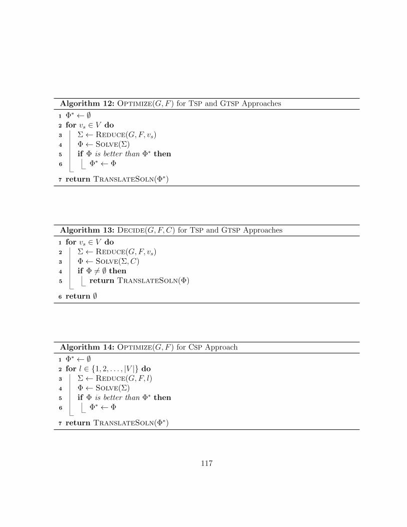
Algorithm 12: Optimize(G,F ) for TSP and GTSP Approaches

1 Φ∗ ← ∅2 for vs ∈ V do3 Σ← Reduce(G,F, vs)4 Φ← Solve(Σ)5 if Φ is better than Φ∗ then6 Φ∗ ← Φ

7 return TranslateSoln(Φ∗)

Algorithm 13: Decide(G,F,C) for TSP and GTSP Approaches

1 for vs ∈ V do2 Σ← Reduce(G,F, vs)3 Φ← Solve(Σ, C)4 if Φ 6= ∅ then5 return TranslateSoln(Φ)

6 return ∅

Algorithm 14: Optimize(G,F ) for CSP Approach

1 Φ∗ ← ∅2 for l ∈ 1, 2, . . . , |V | do3 Σ← Reduce(G,F, l)4 Φ← Solve(Σ)5 if Φ is better than Φ∗ then6 Φ∗ ← Φ


117

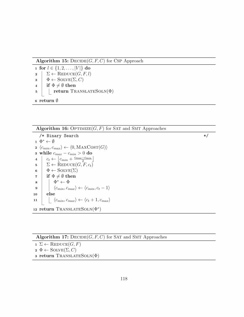
Algorithm 15: Decide(G,F,C) for CSP Approach

1 for l ∈ 1, 2, . . . , |V | do2 Σ← Reduce(G,F, l)3 Φ← Solve(Σ, C)4 if Φ 6= ∅ then5 return TranslateSoln(Φ)

6 return ∅

Algorithm 16: Optimize(G,F ) for SAT and SMT Approaches

/* Binary Search */

1 Φ∗ ← ∅2 〈cmin, cmax〉 ← 〈0,MaxCost(G)〉3 while cmax − cmin > 0 do4 ct ←

⌊cmin + cmax−cmin

2

⌋5 Σ← Reduce(G,F, ct)6 Φ← Solve(Σ)7 if Φ 6= ∅ then8 Φ∗ ← Φ9 〈cmin, cmax〉 ← 〈cmin, ct − 1〉

10 else11 〈cmin, cmax〉 ← 〈ct + 1, cmax〉


Algorithm 17: Decide(G,F,C) for SAT and SMT Approaches

1 Σ← Reduce(G,F )2 Φ← Solve(Σ, C)3 return TranslateSoln(Φ)

118

B.3 Reduction of the Hamiltonian Cycle Problem to

SAT

In this section we reduce the Hamiltonian cycle problem (HCP) aspect of SAT-TSP toSAT (used in Sections B.4.1 and B.4.5 for the SAT and SMT reductions). Specifically, wetranslate the SAT-TSP instance 〈G,F, c =∞〉 to SAT. There are existing translations fromHCP to SAT, however, this translation requires a Hamiltonian cycle of the included verticesV ′ (not necessarily the entire graph).

Our translation is inspired by the IP formulation of the Hamiltonian Cycle Problem(HCP) [47]. The first part of the translation creates a formula F that encodes the Hamilto-nian cycle aspect of the SAT-TSP problem. We start with a set of constraints that capturethe Hamiltonian cycle problem for the included vertices V ′:

L1.1 If 〈vi, vj〉 ∈ E is in the solution, then vi and vj are in the solution.

L1.2 For each vi ∈ V there is at most one outgoing edge in the solution.

L1.3 For vj there is at most one incoming edge in the solution.

L1.4 If vi and vj are in the solution, then vj is reachable from vi. To accomplish this weuse the additional set of indicator variables xv1,0, xv2,0, . . . , xv|V |,0, xv1,1, . . . , xv|V |,|V |.

(a) Exactly one vertex in the set xv1,0, xv2,0, . . . , xv|V |,0 is true.

(b) Vertex vi is in the solution (xvi = 1) if and only if at least one variable in theset xvi,1, xvi,2, . . . , xvi,|V | is true.

(c) Variable xvj ,k+1 = 1 if and only if there exists xvi,k = 1 and 〈vi, vj〉 is in thesolution.

Now we encode these constraints into the SAT formula F using the set of verticesand edges as Boolean variables. As well, we use the set of variables introduced in con-straint L2.4c. The following translates the above constraints into the SAT F .

L2.1 This is encoded with an implies constraint:∧〈vi,vj〉∈E

〈vi, vj〉 =⇒ (vi ∧ vj).

119

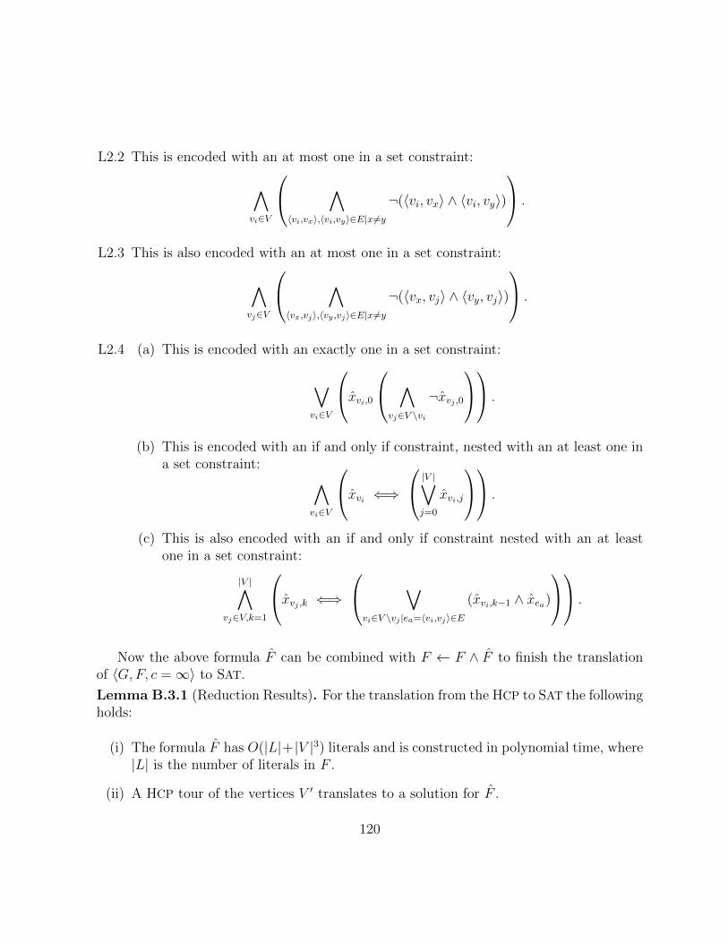
L2.2 This is encoded with an at most one in a set constraint:

∧vi∈V

∧〈vi,vx〉,〈vi,vy〉∈E|x 6=y

¬(〈vi, vx〉 ∧ 〈vi, vy〉)

.

L2.3 This is also encoded with an at most one in a set constraint:

∧vj∈V

∧〈vx,vj〉,〈vy ,vj〉∈E|x 6=y

¬(〈vx, vj〉 ∧ 〈vy, vj〉)

.

L2.4 (a) This is encoded with an exactly one in a set constraint:

∨vi∈V

xvi,0 ∧vj∈V \vi

¬xvj ,0

.

(b) This is encoded with an if and only if constraint, nested with an at least one ina set constraint: ∧

vi∈V

xvi ⇐⇒ |V |∨j=0

xvi,j

.

(c) This is also encoded with an if and only if constraint nested with an at leastone in a set constraint:

|V |∧vj∈V,k=1

xvj ,k ⇐⇒ ∨vi∈V \vj |ea=〈vi,vj〉∈E

(xvi,k−1 ∧ xea)

.

Now the above formula F can be combined with F ← F ∧ F to finish the translationof 〈G,F, c =∞〉 to SAT.

Lemma B.3.1 (Reduction Results). For the translation from the HCP to SAT the followingholds:

(i) The formula F has O(|L|+|V |3) literals and is constructed in polynomial time, where|L| is the number of literals in F .

(ii) A HCP tour of the vertices V ′ translates to a solution for F .

120

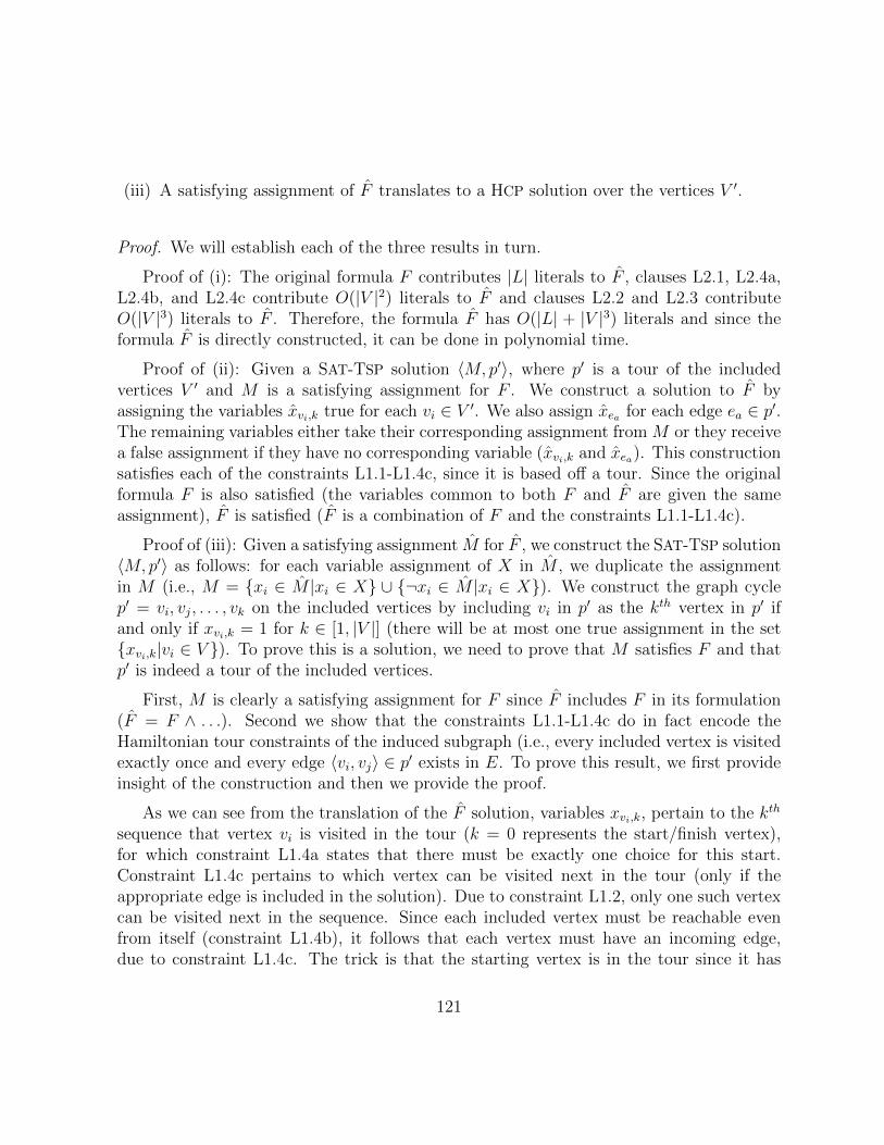
(iii) A satisfying assignment of F translates to a HCP solution over the vertices V ′.

Proof. We will establish each of the three results in turn.

Proof of (i): The original formula F contributes |L| literals to F , clauses L2.1, L2.4a,L2.4b, and L2.4c contribute O(|V |2) literals to F and clauses L2.2 and L2.3 contributeO(|V |3) literals to F . Therefore, the formula F has O(|L| + |V |3) literals and since theformula F is directly constructed, it can be done in polynomial time.

Proof of (ii): Given a SAT-TSP solution 〈M, p′〉, where p′ is a tour of the includedvertices V ′ and M is a satisfying assignment for F . We construct a solution to F byassigning the variables xvi,k true for each vi ∈ V ′. We also assign xea for each edge ea ∈ p′.The remaining variables either take their corresponding assignment from M or they receivea false assignment if they have no corresponding variable (xvi,k and xea). This constructionsatisfies each of the constraints L1.1-L1.4c, since it is based off a tour. Since the originalformula F is also satisfied (the variables common to both F and F are given the sameassignment), F is satisfied (F is a combination of F and the constraints L1.1-L1.4c).

Proof of (iii): Given a satisfying assignment M for F , we construct the SAT-TSP solution〈M, p′〉 as follows: for each variable assignment of X in M , we duplicate the assignmentin M (i.e., M = xi ∈ M |xi ∈ X ∪ ¬xi ∈ M |xi ∈ X). We construct the graph cyclep′ = vi, vj, . . . , vk on the included vertices by including vi in p′ as the kth vertex in p′ ifand only if xvi,k = 1 for k ∈ [1, |V |] (there will be at most one true assignment in the setxvi,k|vi ∈ V ). To prove this is a solution, we need to prove that M satisfies F and thatp′ is indeed a tour of the included vertices.

First, M is clearly a satisfying assignment for F since F includes F in its formulation(F = F ∧ . . .). Second we show that the constraints L1.1-L1.4c do in fact encode theHamiltonian tour constraints of the induced subgraph (i.e., every included vertex is visitedexactly once and every edge 〈vi, vj〉 ∈ p′ exists in E. To prove this result, we first provideinsight of the construction and then we provide the proof.

As we can see from the translation of the F solution, variables xvi,k, pertain to the kth

sequence that vertex vi is visited in the tour (k = 0 represents the start/finish vertex),for which constraint L1.4a states that there must be exactly one choice for this start.Constraint L1.4c pertains to which vertex can be visited next in the tour (only if theappropriate edge is included in the solution). Due to constraint L1.2, only one such vertexcan be visited next in the sequence. Since each included vertex must be reachable evenfrom itself (constraint L1.4b), it follows that each vertex must have an incoming edge,due to constraint L1.4c. The trick is that the starting vertex is in the tour since it has

121

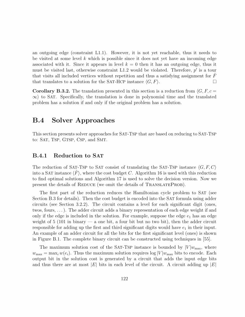
an outgoing edge (constraint L1.1). However, it is not yet reachable, thus it needs tobe visited at some level k which is possible since it does not yet have an incoming edgeassociated with it. Since it appears in level k = 0 then it has an outgoing edge, thus itmust be visited last, otherwise constraint L1.2 would be violated. Therefore, p′ is a tourthat visits all included vertices without repetition and thus a satisfying assignment for Fthat translates to a solution for the SAT-HCP instance 〈G,F 〉.

Corollary B.3.2. The translation presented in this section is a reduction from 〈G,F, c =∞〉 to SAT. Specifically, the translation is done in polynomial time and the translatedproblem has a solution if and only if the original problem has a solution.

B.4 Solver Approaches

This section presents solver approaches for SAT-TSP that are based on reducing to SAT-TSP

to: SAT, TSP, GTSP, CSP, and SMT.

B.4.1 Reduction to SAT

The reduction of SAT-TSP to SAT consist of translating the SAT-TSP instance 〈G,F,C〉into a SAT instance 〈F 〉, where the cost budget C. Algorithm 16 is used with this reductionto find optimal solutions and Algorithm 17 is used to solve the decision version. Now wepresent the details of Reduce (we omit the details of TranslateProb).

The first part of the reduction reduces the Hamiltonian cycle problem to SAT (seeSection B.3 for details). Then the cost budget is encoded into the SAT formula using addercircuits (see Section 3.2.2). The circuit contains a level for each significant digit (ones,twos, fours, . . . ). The adder circuit adds a binary representation of each edge weight if andonly if the edge is included in the solution. For example, suppose the edge e1 has an edgeweight of 5 (101 in binary — a one bit, a four bit but no two bit), then the adder circuitresponsible for adding up the first and third significant digits would have e1 in their input.An example of an adder circuit for all the bits for the first significant level (ones) is shownin Figure B.1. The complete binary circuit can be constructed using techniques in [55].

The maximum solution cost of the SAT-TSP instance is bounded by |V |wmax, wherewmax = maxiw(ei). Thus the maximum solution requires log |V |wmax bits to encode. Eachoutput bit in the solution cost is generated by a circuit that adds the input edge bitsand thus there are at most |E| bits in each level of the circuit. A circuit adding up |E|

122

These carry over bits are used as inputin the next level of adder circuit.

XOR gate.

AND gate.

2-Bit Adder circuits

Figure B.1: An adder circuit summing up xc0 , the one-bits of the solution cost. In thisinstance the edges e1, e3, e4, e8, e9 have odd edge weights and all other edges have evenweights.

bits would require at most |E| 2-bit adder circuits (an XOR and an AND gate shown inFigure B.1). Therefore, the complete adder circuit is of size O(|E| log |V |wmax) and usingmethods from [41] this circuit is efficiently translated to a Boolean formula.

The cost budget constraints are constructed by forcing an assignment on a subsetof the solution cost bits (variables) xc0 , xc1 , . . . , xcn, where the total solution cost isc =

∑ni=0 2ixci . For example, if we wish to find a solution of cost seven or less, then all

variables representing powers of three and higher are forced to be false. All cost constraintsthat use this approach are of size O(log(|V |wmax)).

B.4.2 Reduction to TSP

The reduction of SAT-TSP to TSP consist of translating the SAT-TSP instance 〈G,F,C〉 toa series of TSP instances Gvs , where the vertex vs is assumed to be in the solution. Algo-rithm 12 is used to find optimal solutions and Algorithm 13 is used to solve decision prob-lems. Now we present the details of Reduce (we omit the details of TranslateProb).

This reduction is inspired by the translation of SAT to the Hamiltonian Cycle Prob-lem [47]. The first step in expressing F as a graph G with the assumption that vs is inthe solution, is to create a chain of vertices for each variable xi ∈ X, for which we refer toas widget Ωxi . The direction that the TSP solution traverses the widget (chain) indicatesthe assignment of the SAT variable — traverse the widget Ωxi from left to right then the

123

variable xi = 1 (true), traverse the widget from right to left then xi = 0 (false). Once thesolution tour starts traversing the widget it cannot change directions and it must finishvisiting the widget before moving onto the next widget. Figure B.2 shows an example ofa widget and its connections.

The TSP graph Gvs construction also includes a vertex vci for each clause ci ∈ C inthe formula F . The widget construction allows us to connect the clause vertices so thetour can only visit the clause vertex only if the clause would be satisfied by the variableassignment for the widget. For example, suppose clause c1 = (x1 ∨ x2 ∨ ¬x3), then theclause vertex vc1 is only connected to widgets Ωx1 , Ωx2 and Ωx3 and it can only be visitedif the tour traverses Ωx1 or Ωx2 from left to right, or if the tour traverses Ωx3 from right toleft.

The the widgets are connected to each other to ensure feasible tours visit all the includedvertices first (any widget Ωxvi

that is traversed left to right that corresponds with xvi forvi ∈ V ), then the non-included vertices, and then the auxiliary variable widgets. In thisway, as the solution visits widgets that represent included vertices in Gvs , it does so withthe same costs as if it were visiting vertices in G. This is accomplished by restricting theset of incoming and outgoing edges to the widgets. Figure B.3 shows how the widgets areconnected to each other. With this construction a TSP solution of cost c translates to aSAT-TSP solution of cost c.

The details of this approach and the proof of its correctness are given in our preliminarywork [39]. For the sake of conciseness and since this approach is not among the mostsuccessful, we refer the reader to our earlier work for more details [39].

2 3 4 5 6 7 81 9

Figure B.2: An example of the widget Ωxi . In this instance the only clauses in F thatcontain the variable xi are clauses c1 and c2. The clause c1 contains the literal x1 andc2 contains the literal ¬xi. A TSP solution that traverses the widget from left to right(1 → 9) indicates that xi = 1 in the SAT-TSP solution and a solution that traverses thewidget from right to left (9→ 1) indicates that xi = 0.

124

Figure B.3: The connections between widgets in the TSP graph. Dotted edges have zeroweight. An edge going into or out of the left of the widget indicates a connection to leftmost vertex in the widget chain. Likewise, an edge going into or out of the right sideindicates a connection to the right most vertex in the chain.

B.4.3 Reduction to GTSP

The reduction of SAT-TSP to GTSP consist of translating the SAT-TSP instance 〈G,F,C〉to a series of GTSP instances that assume a specific vertex vs, is included in the solu-tion. Algorithm 12 is used to find optimal solutions and Algorithm 13 is used to solvedecision problems. Now we present the details of Reduce (we omit the details of Trans-lateProb).

The reduction consist of creating a graph that contains vertices to represent the literalsin F , sets to represent assignment of variables (true or false), and sets to represent clausesatisfaction (at least one literal in each clause must be true). In this construction visitinga vertex literal translates to an assignment of the variable (true or false) and visiting a setthat is associated with a clause, translates to a satisfying the clause.

The sets in the GTSP instance are used to restrict the assignments of the variable xi ∈ F— each variable can only be assigned true or false — not both. This is accomplished bycreating a vertex vxi to represent the true assignment of xi and a vertex v¬xi to representthe false assignment of xi. We classify these vertices as root vertices. Creating the setvxi , v¬xi for each variable in the formula ensures that the GTSP solution can only visiteither the true vertex vxi or the false vertex v¬xi . The sets are also used to ensure thateach clause ci ∈ F is satisfied. This is accomplished by creating a set for each clause.However, a clause ci may be satisfied by multiple literals where a GTSP solution can only

125

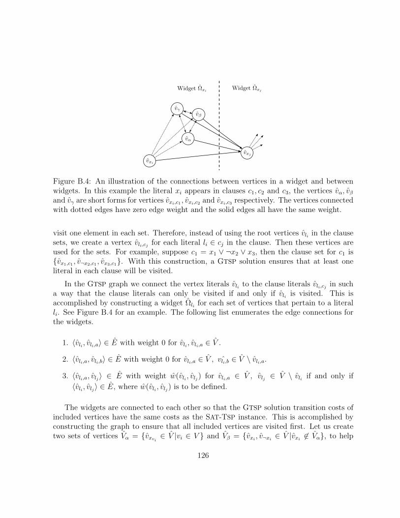
Figure B.4: An illustration of the connections between vertices in a widget and betweenwidgets. In this example the literal xi appears in clauses c1, c2 and c3, the vertices vα, vβand vγ are short forms for vertices vxi,c1 , vxi,c2 and vxi,c3 respectively. The vertices connectedwith dotted edges have zero edge weight and the solid edges all have the same weight.

visit one element in each set. Therefore, instead of using the root vertices vli in the clausesets, we create a vertex vli,cj for each literal li ∈ cj in the clause. Then these vertices areused for the sets. For example, suppose c1 = x1 ∨ ¬x2 ∨ x3, then the clause set for c1 isvx1,c1 , v¬x2,c1 , vx3,c1. With this construction, a GTSP solution ensures that at least oneliteral in each clause will be visited.

In the GTSP graph we connect the vertex literals vli to the clause literals vli,cj in sucha way that the clause literals can only be visited if and only if vli is visited. This isaccomplished by constructing a widget Ωli for each set of vertices that pertain to a literalli. See Figure B.4 for an example. The following list enumerates the edge connections forthe widgets.

1. 〈vli , vli,a〉 ∈ E with weight 0 for vli , vli,a ∈ V .

2. 〈vli,a, vli,b〉 ∈ E with weight 0 for vli,a ∈ V , ˆvli,b ∈ V \ vli,a.

3. 〈vli,a, vlj〉 ∈ E with weight w(vli , vlj) for vli,a ∈ V , vlj ∈ V \ vli if and only if

〈vli , vlj〉 ∈ E, where w(vli , vlj) is to be defined.

The widgets are connected to each other so that the GTSP solution transition costs ofincluded vertices have the same costs as the SAT-TSP instance. This is accomplished byconstructing the graph to ensure that all included vertices are visited first. Let us createtwo sets of vertices Vα = vxvi ∈ V |vi ∈ V and Vβ = vxi , v¬xi ∈ V |vxi 6∈ Vα, to help

126

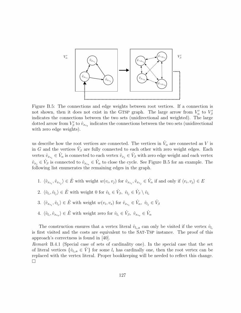
Figure B.5: The connections and edge weights between root vertices. If a connection isnot shown, then it does not exist in the GTSP graph. The large arrow from V ′α to V ′βindicates the connections between the two sets (unidirectional and weighted). The largedotted arrow from V ′β to vxvs indicates the connections between the two sets (unidirectionalwith zero edge weights).

us describe how the root vertices are connected. The vertices in Vα are connected as V isin G and the vertices Vβ are fully connected to each other with zero weight edges. Each

vertex vxvi ∈ Vα is connected to each vertex vxj ∈ Vβ with zero edge weight and each vertex

vxj ∈ Vβ is connected to vxvs ∈ Vα to close the cycle. See Figure B.5 for an example. Thefollowing list enumerates the remaining edges in the graph.

1. 〈vxvi , vxvj 〉 ∈ E with weight w(vi, vj) for vxvi , vxvj ∈ Vα if and only if 〈vi, vj〉 ∈ E

2. 〈vli , vlj〉 ∈ E with weight 0 for vli ∈ Vβ, vlj ∈ Vβ \ vli

3. 〈vxvi , vlj〉 ∈ E with weight w(vi, vs) for vxvi ∈ Vα, vlj ∈ Vβ

4. 〈vli , vxvs 〉 ∈ E with weight zero for vli ∈ Vβ, vxvs ∈ Vα

The construction ensures that a vertex literal vli,a can only be visited if the vertex vliis first visited and the costs are equivalent to the SAT-TSP instance. The proof of thisapproach’s correctness is found in [40].

Remark B.4.1 (Special case of sets of cardinality one). In the special case that the setof literal vertices vli,a ∈ V for some li has cardinally one, then the root vertex can bereplaced with the vertex literal. Proper bookkeeping will be needed to reflect this change.

127

B.4.4 Reduction to CSP

The reduction of SAT-TSP to CSP consist of translating the SAT-TSP instance 〈G,F,C〉to a series of CSP instances that assume that the set of included vertices V ′ is of a spe-cific size. Algorithm 14 is used to find optimal solutions and Algorithm 15 is used tosolve decision problems. Now we present the details of Reduce (we omit the details ofTranslateProb).

The reduction consist of expressing the graph as a weight matrix in the CSP format,translating the formula F into a CSP formula [96], and reducing a fixed length Hamiltoniancycle problem to CSP. The expression of the fixed length Hamiltonian cycle problem is asfollows: first create a fixed length vector to represent the tour, next each variable in thetour vector is constrained to take on values i|vi ∈ V [G], and finally each element in thetour vector is constrained to be all different to ensure that no duplicate entries show up inthe cycle. Additionally, there is a set of simple constraints used to link the tour vector withthe weight matrix such that the solution cost can be calculated and constrained (vertex viis included in the tour if and only if variable xi = 1).

B.4.5 Reduction to SMT

The reduction of SAT-TSP to SMT consist of translating the SAT-TSP instance 〈G,F,C〉into an SMT instance with a cost budget C. Algorithm 16 is used with this reduction tofind optimal solutions and Algorithm 17 is used to solve the decision version. Now wepresent the details of Reduce (we omit the details of TranslateProb).

Like the SAT reduction, this reduction reduces the HCP to SAT (Section B.3). The costis encoded and constrained using an SMT arithmetic theory. This saves O(log cmax) workcompared to the SAT approach. The formulas used in calculating and constraining thecosts are as follows: an edge ei contributes w(ei) to the solution cost c′ if and only if xeiis assigned true in the formula. The binary search algorithm chooses a budget cost c andthe constraint c′ ≤ c is encoded into the SMT instance. If the SMT solver finds a solutionthen the edge variables are translated into a SAT-TSP tour and the remaining variableassignments are used to construct a satisfying assignment for F .

B.5 Benchmark Problems

In this section we detail the construction of the problem instances in the benchmark (theseproblems are different than the problems found in the main body of thesis).

128

The problems in libraries SetLib, CountLib, OrderedLib, and MultiRobotLibuse the following environments.

The Metric Library Environment The robot is able to move within the two dimen-sional space x ∈ [0, 1] and y ∈ [0, 1] and a set of locations are uniformly randomly placedwithin the square. There is one location chosen at random to represent the robot’s home.The rest of the locations contain items for the robot to retrieve. Each location has oneitem with a random shape and colour. The items can take one of eight colours and oneof thee shapes. The graph is constructed to capture the euclidean distance between thelocations.

The Non-Metric Library Environment The robot’s environment graph is con-structed with uniform random edge weights in the domain [0, 1]. One vertex is randomlychosen for the robot’s home. The rest are item locations. Each location has one itemwith a random shape and colour. The items can take one of eight colours and one of theeshapes.

Remark B.5.1 (Vertex labels). In the rest of this section it will be convenient for us to talkabout the set of vertices that have a specific shape or colour. We let the set Vlabel representthe set of vertices with that label (shape, colour, or other).

B.5.1 SatLib

To test how well each approach performs on solving highly constrained SAT instances,we translated SAT instances from the SatLib library [37] into SAT-TSP instances. Theconstruction of the SAT-TSP instances is as follows: create a fully connected undirectedgraph G with |V | vertices of zero edge weight and force each vertex to be included in thesolution, F ← F ∧(xv1∧xv2∧. . .). Then the SAT-TSP instance 〈G,F, c = 0〉 is equivalent tothe SAT instance F . The optimization version of the SAT-TSP translation is also equivalentto the SAT instance since every solution for the SAT-TSP instance has a cost of zero (everysolution is optimal). There are 41 instances in this library ranging in size from 20 to 600variables in the formula F .

B.5.2 TspLib

To test how well each approach performs on simple patrolling problems, we translated TSP

instances from the TspLib [77] into SAT-TSP instances. The construction of the SAT-TSP

129

instances is as follows: create a formula F = (xv1 ∧ xv2 ∧ . . . ∧ xv|V |). Notice that there isonly one solution to the formula F (include every vertex in the solution), thus the SAT-TSP

instance 〈G,F 〉 is equivalent to the TSP instance 〈G〉. There are 66 instances in this libraryranging in size from 16 to 1379 vertices.

B.5.3 HardLib

We also created highly-constrained planning problems with complex environments by com-bining instances from the SatLib and TspLib libraries. The SAT-TSP instances 〈G,F 〉uses the formula F from the SAT instance and the graph G from the TSP instance forcombinations that satisfy |X| ≥ |V |. There are 348 instances in this library.

B.5.4 SetLib

We created the SetLib library to test how well each solver performs on nested set problems.The problem instances are randomly generated as described in the metric and non-metriclibrary environments. The problem is constrained to have one item of each shape, all thesame colour in the solution. There are 200 problem instances in this library ranging in sizefrom 10 to 100 vertices.

B.5.5 GTspLib

To test how well each approach performs on one-in-a-set routing problems or similar prob-lems, we translated GTSP instances from the GTspLib library [30] to SAT-TSP instances〈G,F 〉 where,

F =

|S|∧j=1

∨vi∈Sj

xvi

.

There are 83 instances in this library ranging in size from 17 to 1084 vertices in the graph.

B.5.6 GTspLib+

We created the GTspLib+ library to test how well each approach performs on GTSP

instances with additional SAT constraints. The problem instances are randomly generatedas described in the metric and non-metric library environments. The GTSP sets are of

130

random size with random non-overlapping membership. There are 0 to 200 additionalconstraints of the form: negation, ¬(vi ∧ vj) or implication, (vi =⇒ vj). There are 262instances in this library ranging in size from 10 to 500 vertices.

B.5.7 CountLib

The robot is required to retrieve exactly one cube, at most three spheres, and at least fivecylinders from its environment. The problem instances are randomly generated as describedin the metric and non-metric library environments. These problems are constrained toretrieve an exact but random number of items for each shape (uniformly chosen from theset of possibilities). There are 200 instances in this library ranging in size from 10 to 100vertices.

The problems are translated to SAT-TSP using adder circuits.

B.5.8 OrderedLib

These problem instances are pickup and delivery problems. The environments are gener-ated as in the metric and non-metric library environments, however, the item assignmentsare different. Specifically, the environment locations are a collection of pickup vi and dropoff locations vj (chosen at random) — vi is paired with vj. The robot must visit all thelocations. For every pickup and delivery pair vi, vj the tour must visit vi before vj. Thereare 200 instances in this library ranging in size from 10 to 100 vertices.

These problems are translated to SAT-TSP instances by using the structure in Re-mark 3.4.10. Specifically, the graph is constructed with a series of widgets. When sepa-rated from the rest of the graph, each widget is simply an induced subgraph of the robot’senvironment G. The first widget Ω0, contains only the vertex vs (the home) and the re-maining widgets Ω1, Ω2, . . ., contain the vertices V \ vs. The widgets are connected withdirected edges so that the path may visit them only in increasing order according of theirindex. Figure B.6, Figure B.7, and the following list details how the widgets are connected.First we require some notation: let the vertex label vji represent the vertex vi in widget Ωj.

1. 〈vλi , vγj 〉 ∈ E with weight w(vi, vj) for vλi , v

γj ∈ V , γ ≥ λ if and only if 〈vi, vj〉 ∈ E

2. 〈vλi , v0s〉 ∈ E with weight w(vλi , v

0s) = 0 for all vλi ∈ V \ v0

s

131

The entire graph has O(|V |2) vertices and O(|V |2|E|) edges.

If the SAT-TSP solution visits one of the copies of vertex vi in one of the widgets, thenthe solution visits vi. To ensure that this happens at most once, we use an at-most-one-in-a-set constraint. To ensure the vertex ordering constraints are satisfied, we negate everypair of vertices that violate the ordering. For example, suppose vertex vi must precedevertex vj in the solution. That means for every pair vλi and vσj such that λ ≥ σ we add thenegation clause ¬(xvλi ∧ xvσj ) to the formula. There are O(|V |2) such negation clauses foreach ordering constraint.

In the case that we have precedence constraints for a set of vertices A =va1 , va2 , . . . , va|A| and a set B = vb1 , vb2 , . . . , vb|B|, such that every vertex va ∈ A mustprecede every vertex vb ∈ B, then we use indicator variables to reduce the number of nega-tion clauses from O(|A||B||V |2) to O(|V |2). For example, the set of indicator variables

xλA ∈ x0A, x

1A, . . . , x

|V |A and xλB ∈ x0

B, x1B, . . . , x

|V |B are used to represent a vertex in set A

or B while being visited in widget λ respectively (logic below).

(xv1a1∨ xv1

a2∨ . . . ∨ xv1

a|A|) =⇒ x1

A

Then we negate the indicators instead of the vertex pairs to produce O(|V |2) negationclauses instead of O(|V |2) for each unique pair vi, vj such that vi ∈ A and vj ∈ B.

A solution to the above expression is a solution to the ordered problem since all sub-graphs derived from solutions cannot violate the ordering constraints. The solution also hasthe equivalent cost since the corresponding transitions in G are equivalent to transitionsin G.

B.5.9 MultiRobotLib

A team of robots is tasked with working together to collect at least one item of each colourand at least one item of each shape from the environment. The problem instances arerandomly generated as described in the metric and non-metric library environments. Eachproblem instance has a robot team of random size ranging from two to ten robots. Thereare 200 instances in this library ranging in size from 10 to 100 vertices.

These problems are translated to SAT-TSP instances by using the structure in Re-mark 3.4.10. Specifically, we construct a graph to contain a widget for each robot. Thewidgets Gr are the induced subgraph of the robot’s environment with vertices V \vs, wherevs is the robot’s home location. The graph additionally contains the vertices vr for eachrobot to represent its home. The edges are constructed to force the tour to visit each

132

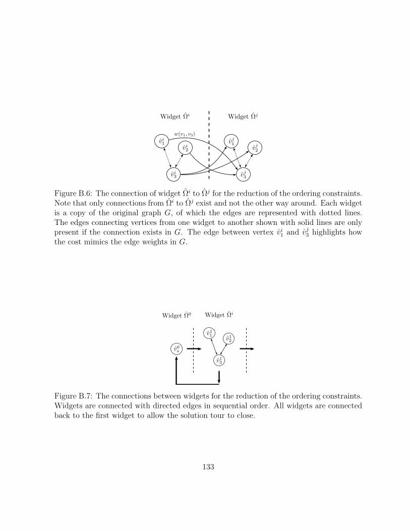
Figure B.6: The connection of widget Ωi to Ωj for the reduction of the ordering constraints.Note that only connections from Ωi to Ωj exist and not the other way around. Each widgetis a copy of the original graph G, of which the edges are represented with dotted lines.The edges connecting vertices from one widget to another shown with solid lines are onlypresent if the connection exists in G. The edge between vertex vi1 and vj3 highlights howthe cost mimics the edge weights in G.

Figure B.7: The connections between widgets for the reduction of the ordering constraints.Widgets are connected with directed edges in sequential order. All widgets are connectedback to the first widget to allow the solution tour to close.

133

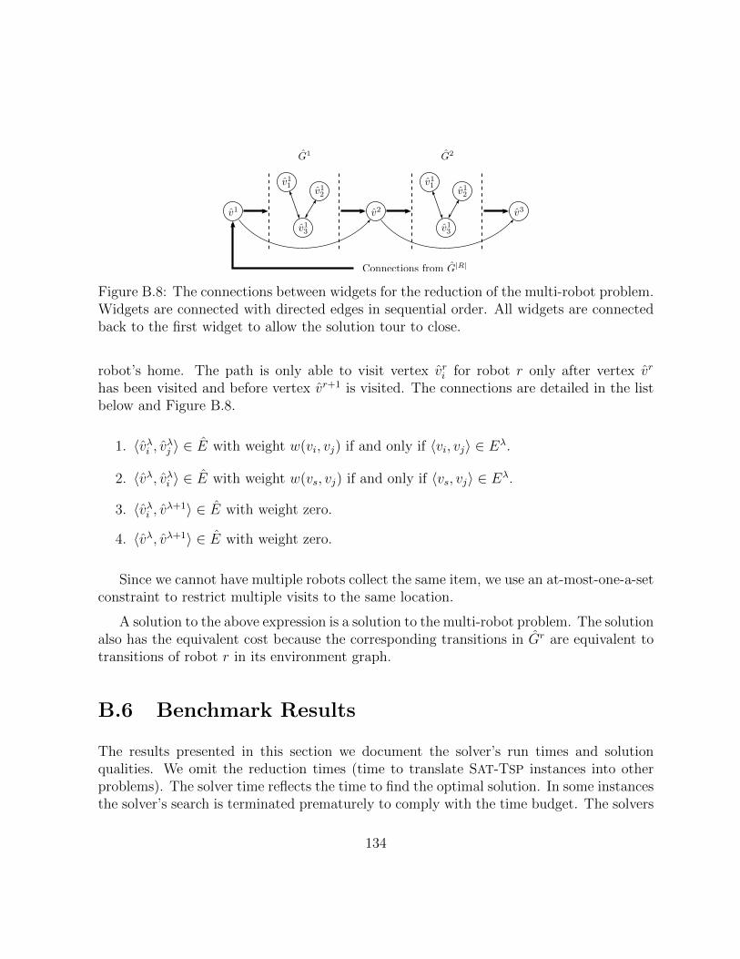
Figure B.8: The connections between widgets for the reduction of the multi-robot problem.Widgets are connected with directed edges in sequential order. All widgets are connectedback to the first widget to allow the solution tour to close.

robot’s home. The path is only able to visit vertex vri for robot r only after vertex vr

has been visited and before vertex vr+1 is visited. The connections are detailed in the listbelow and Figure B.8.

1. 〈vλi , vλj 〉 ∈ E with weight w(vi, vj) if and only if 〈vi, vj〉 ∈ Eλ.

2. 〈vλ, vλi 〉 ∈ E with weight w(vs, vj) if and only if 〈vs, vj〉 ∈ Eλ.

3. 〈vλi , vλ+1〉 ∈ E with weight zero.

4. 〈vλ, vλ+1〉 ∈ E with weight zero.

Since we cannot have multiple robots collect the same item, we use an at-most-one-a-setconstraint to restrict multiple visits to the same location.

A solution to the above expression is a solution to the multi-robot problem. The solutionalso has the equivalent cost because the corresponding transitions in Gr are equivalent totransitions of robot r in its environment graph.

B.6 Benchmark Results

The results presented in this section we document the solver’s run times and solutionqualities. We omit the reduction times (time to translate SAT-TSP instances into otherproblems). The solver time reflects the time to find the optimal solution. In some instancesthe solver’s search is terminated prematurely to comply with the time budget. The solvers

134

are given time budgets in 60 second intervals (60, 120, 180, . . . , 900). We report only thesolver’s best solution with the best time. The simulations were executed on the clustercomputing resource SHARCNET1, which we used more than five years of computing time.

To evaluate each solver approach we use point plots and bar graphs. Both of these plot-s/graphs use a categorization scheme of the solution qualities which is found in Tables B.1and B.2 respectively. We also compare the performance and/or quality to metadata forsome of the approaches. We present this data only when the comparison reveals a corre-lation between performance and/or quality with respect to the metadata. Such metadatamay be the total number of feasible solutions for the SAT-TSP instance or the number ofadditional constraints that have been added to the GTspLib+ instance (Section B.5.6).

Solution Category: DescriptionA : Solutions that achieve the best known cost.B : Solutions that achieve a solution cost within two times the best known

cost, but not the best cost.C : Solutions that have cost worse than two times the best known cost.

Table B.1: Descriptions of the mutually exclusive solution categories used in Figures B.9to B.13.

B.6.1 The Unsuccessful Approaches (SAT, TSP and SMT)

Three of the proposed approaches: SAT, TSP and SMT were unsuccessful compared to theother approaches (see Figure B.14). We developed the SAT and TSP approaches to explorehow well SAT solvers and TSP solvers could respectively handle the addition of TSP andSAT problems. It turns out that both approaches performed poorly. Furthermore, the TSP

approach performed poorly on TSP problems encoded as SAT-TSP problems. This forcesus to conclude that our TSP reductions introduce additional complexity into the problem,which was needed to handle the SAT formula. Thus, it is unlikely that a pure TSP approachwould be a good candidate for SAT-TSP problems.

We developed the SMT approach to allow for partial tour negations as in the CBTSP

approach. However, it suffers a O(|V |3) increase in size due the translation of the Hamil-tonian cycle problem (the SAT approach also suffers from this size increase). We suspectthat this size increase is a contributing factor to its inefficiency.

1https://www.sharcnet.ca

135

https://www.sharcnet.ca

B.6.2 GTSP Approach

The GTSP approach reduces a SAT-TSP instance to |V | TSP instances, where each instancehas a different assumption of which vs ∈ V is in the solution. It uses the GTSP solver,GLNS [88], to find optimal tours. The best result out of the |V | solutions is used. Thesolver divides the time budget evenly among each GTSP instance and it takes the timebudget as input to terminate itself.

Strengths We developed the GTSP approach to help solve GTSP like problems as severalof the proposed approaches perform poorly on these types of problems. As we had hoped,this approach does perform well on GTSP and GTSP-like instances (TspLib, GTspLiband GTspLib+). Figures B.15b, B.16a and B.16b compile the results for this approach.

Figure B.14 shows that this approach is able to find a number of the best knownsolutions and Figure B.9a shows that if it does find the optimal solution then it is oftenthe best performer.

Weaknesses The GTSP approach was not designed to handle highly constrained prob-lems such as SAT or counting problems. Thus this approach struggles with such problems,which is shown in Figures B.15a, B.15c, B.17a, B.17b, and B.18b.

Figure B.9b) shows that this approach degrades as the GTSP-like instances become lessGTSP like.

B.6.3 CSP Approach

The CSP approach reduces a SAT-TSP instance to |V | CSP instances each with a differentassumption of the solution tour size. It uses the CSP solver Gecode [85] to find the optimalsolution of each translation and the best result is used. The CSP approach divides the timebudget evenly among each CSP instance and the CSP solver takes the time budget as inputto terminate itself.

Strengths We developed the CSP approach because it is relatively easy to express logicand optimization problems. Additionally, CSP solvers are relatively good at finding solu-tions, which we can see from Figure B.14.

136

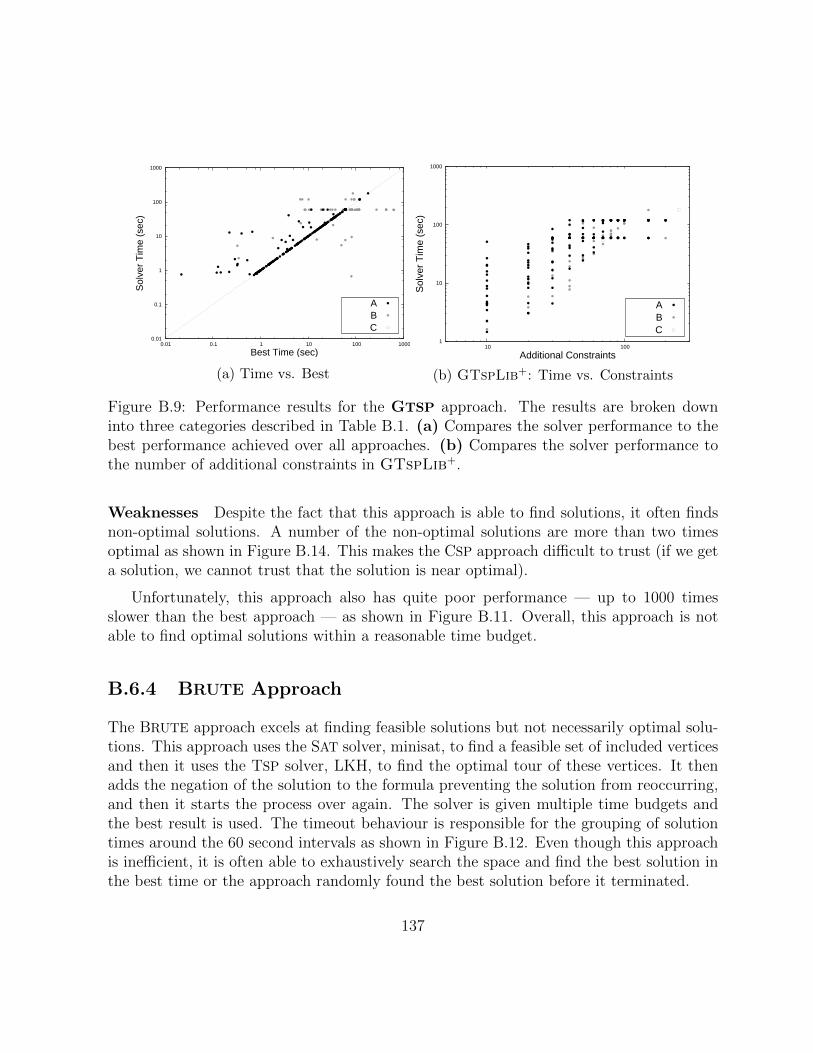
0.01

0.1

1

10

100

1000

0.01 0.1 1 10 100 1000

Sol

ver

Tim

e (s

ec)

Best Time (sec)

CBA

(a) Time vs. Best

1

10

100

1000

10 100

Sol

ver

Tim

e (s

ec)

Additional Constraints

CBA

(b) GTspLib+: Time vs. Constraints

Figure B.9: Performance results for the GTSP approach. The results are broken downinto three categories described in Table B.1. (a) Compares the solver performance to thebest performance achieved over all approaches. (b) Compares the solver performance tothe number of additional constraints in GTspLib+.

Weaknesses Despite the fact that this approach is able to find solutions, it often findsnon-optimal solutions. A number of the non-optimal solutions are more than two timesoptimal as shown in Figure B.14. This makes the CSP approach difficult to trust (if we geta solution, we cannot trust that the solution is near optimal).

Unfortunately, this approach also has quite poor performance — up to 1000 timesslower than the best approach — as shown in Figure B.11. Overall, this approach is notable to find optimal solutions within a reasonable time budget.

B.6.4 BRUTE Approach

The BRUTE approach excels at finding feasible solutions but not necessarily optimal solu-tions. This approach uses the SAT solver, minisat, to find a feasible set of included verticesand then it uses the TSP solver, LKH, to find the optimal tour of these vertices. It thenadds the negation of the solution to the formula preventing the solution from reoccurring,and then it starts the process over again. The solver is given multiple time budgets andthe best result is used. The timeout behaviour is responsible for the grouping of solutiontimes around the 60 second intervals as shown in Figure B.12. Even though this approachis inefficient, it is often able to exhaustively search the space and find the best solution inthe best time or the approach randomly found the best solution before it terminated.

137

0.01

0.1

1

10

100

1000

0.01 0.1 1 10 100 1000

Sol

ver

Tim

e (s

ec)

Best Time (sec)

CBA

Figure B.10: CSP (Gecode)

Figure B.11: Performance results of the CSP approach on the simulation library. Theresults are broken down into three categories described in Table B.1.

Strengths The BRUTE approach provides a straightforward method to leverage the bestperforming SAT and TSP solvers. As shown in Figure B.14 the approach is frequently ableto find the best known solution and it often outperforms the other approaches. A goodproperty of this solver is that if the solver quits before the time budget is exceeded and theTSP solver is an exact solver such as Concorde [3], then it has found the optimal solution.Our implementation uses LKH which sometimes returns sub-optimal solutions (LKH ismore efficient than Concorde and has very good performance). We see this behaviourin Figures B.12a by observing that all the results below 60 seconds are the best knownsolutions (category A).

Figure B.15b verifies that this approach is the best choice for solving instances in theTspLib. This is not surprising, since the SAT formula in the SAT-TSP instance only hasone solution to search. For such instances, the brute approach quickly solves the SATformula and then uses the TSP solver, LKH, to solve the TSP problem.

Weaknesses This approach searches all of the SAT solutions and only after it has ex-plored each solution does it provide the optimal result. If the search is prematurely termi-nated (timed out), the solution quality can vary wildly. As such the solver’s run time isheavily dependent on how many solutions it searches. Figure B.12b verifies this correlation.

This approach struggles GTspLib, SetLib and CountLib instances since they havea large number of feasible solutions to search (see Figures B.16a-B.17b).

138

0.01

0.1

1

10

100

1000

0.01 0.1 1 10 100 1000

Sol

ver

Tim

e (s

ec)

Best Time (sec)

CBA

(a) Time vs. Best

0.01

0.1

1

10

100

1000

1 10 100 1000

Sol

ver

Tim

e (s

ec)

Number of Solutions

CBA

(b) Time vs. Solutions

Figure B.12: Performance results of the BRUTE approach on the full library. Results aredivided into categories described in Table B.1. (a) Compares the solver time to the bestperformance achieved over all approaches for SAT-TSP instances. (b) Compares the solvertime to the number of SAT-TSP solutions of the instance.

0.01

0.1

1

10

100

1000

0.01 0.1 1 10 100 1000

Sol

ver

Tim

e (s

ec)

Best Time (sec)

CBA

(a) Time vs. Best

0.001

0.01

0.1

1

10

100

1000

1 10 100 1000

Sol

ver

Tim

e (s

ec)

Number of Solutions

CBA

(b) Time vs. Solutions

Figure B.13: Performance results of the CBTSP approach on the simulation library. Theresults are broken down into three categories described in Table B.1. (a) Compares thesolver time to the best performance achieved over all approaches. (b) Compares the solvertime to the number of SAT-TSP solutions of the instance.

139

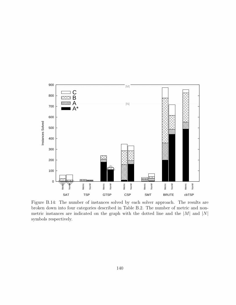
0

100

200

300

400

500

600

700

800

900

Met

ric

Non

M

Met

ric

Non

M

Met

ric

Non

M

Met

ric

Non

M

Met

ric

Non

M

Met

ric

Non

M

Met

ric

Non

M

Inst

ance

s S

olve

d

A*ABC

|M|

|N|

cbTSPBRUTESMTCSPGTSPTSPSAT

Figure B.14: The number of instances solved by each solver approach. The results arebroken down into four categories described in Table B.2. The number of metric and non-metric instances are indicated on the graph with the dotted line and the |M | and |N |symbols respectively.

140

0

5

10

15

20

25

30

35

40

45M

etric

Non

M

Met

ric

Non

M

Met

ric

Non

M

Met

ric

Non

M

Inst

ance

s S

olve

d

A*ABC |M|

cbTSPBRUTECSPGTSP

(a) SatLib

0

10

20

30

40

50

60

70

Met

ric

Non

M

Met

ric

Non

M

Met

ric

Non

M

Met

ric

Non

M

Inst

ance

s S

olve

d

A*ABC

|M|

|N|

cbTSPBRUTECSPGTSP

(b) TspLib

0

20

40

60

80

100

120

140

160

180

Met

ric

Non

M

Met

ric

Non

M

Met

ric

Non

M

Met

ric

Non

M

Inst

ance

s S

olve

d

A*ABC

|M|

|N|

cbTSPBRUTECSPGTSP

(c) HardLib

Figure B.15: The number of instances solved in their respective library by each successfulsolver approach. The results are broken down into four categories described in Table B.2.The number of metric and non-metric instances are indicated on each graph with thedotted line and the |M | and |N | symbols respectively (there are no non-metric instancesin SatLib).

141

0

10

20

30

40

50

60

70

80

Met

ric

Non

M

Met

ric

Non

M

Met

ric

Non

M

Met

ric

Non

M

Inst

ance

s S

olve

d

A*ABC |M|

|N|

cbTSPBRUTECSPGTSP

(a) GTspLib

0

20

40

60

80

100

120

140

Met

ric

Non

M

Met

ric

Non

M

Met

ric

Non

M

Met

ric

Non

M

Inst

ance

s S

olve

d

A*ABC |M|,|N|

cbTSPBRUTECSPGTSP

(b) GTspLib+

Figure B.16: The number of instances solved in their respective library by each successfulsolver approach. The results are broken down into four categories described in Table B.2.The number of metric and non-metric instances are indicated on each graph with thedotted line and the |M | and |N | symbols respectively.

142

0

20

40

60

80

100

Met

ric

Non

M

Met

ric

Non

M

Met

ric

Non

M

Met

ric

Non

M

Inst

ance

s S

olve

d

A*ABC

|M|,|N|

cbTSPBRUTECSPGTSP

(a) SetLib

0

20

40

60

80

100

Met

ric

Non

M

Met

ric

Non

M

Met

ric

Non

M

Met

ric

Non

M

Inst

ance

s S

olve

d

A*ABC

|M|,|N|

cbTSPBRUTECSPGTSP

(b) CountLib


143

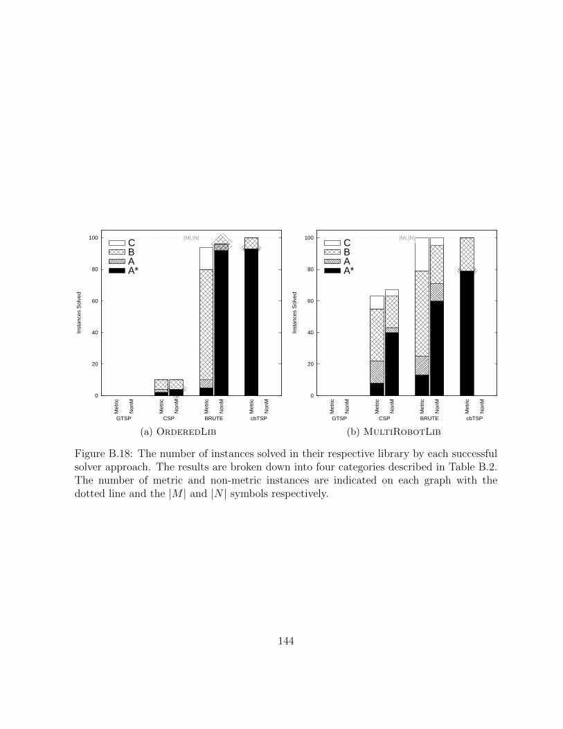
0

20

40

60

80

100

Met

ric

Non

M

Met

ric

Non

M

Met

ric

Non

M

Met

ric

Non

M

Inst

ance

s S

olve

d

A*ABC

|M|,|N|

cbTSPBRUTECSPGTSP

(a) OrderedLib

0

20

40

60

80

100

Met

ric

Non

M

Met

ric

Non

M

Met

ric

Non

M

Met

ric

Non

M

Inst

ance

s S

olve

d

A*ABC

|M|,|N|

cbTSPBRUTECSPGTSP

(b) MultiRobotLib


144

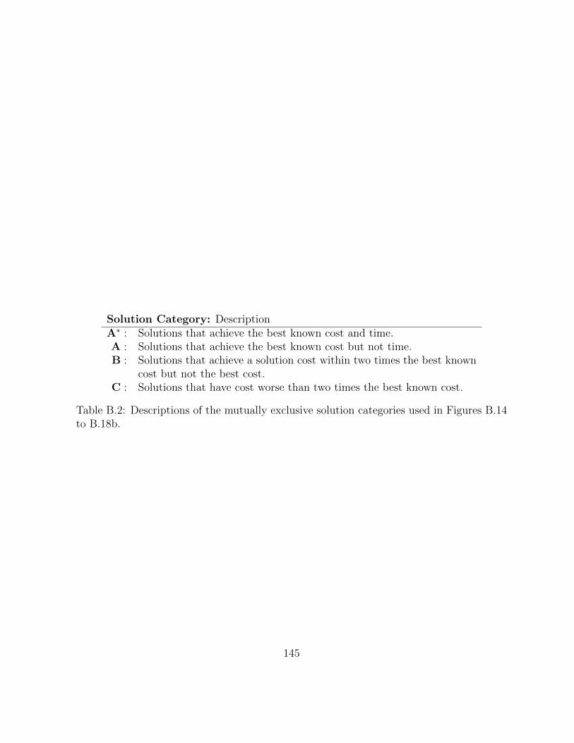
Solution Category: DescriptionA∗ : Solutions that achieve the best known cost and time.A : Solutions that achieve the best known cost but not time.B : Solutions that achieve a solution cost within two times the best known

cost but not the best cost.C : Solutions that have cost worse than two times the best known cost.

Table B.2: Descriptions of the mutually exclusive solution categories used in Figures B.14to B.18b.

145

Robotic Path Planning for High-Level Tasks in Discrete ...

Documents

Transcript of Robotic Path Planning for High-Level Tasks in Discrete ...