Planning and Control Methods for Robotic Manipulation Tasks ...
135
Lehrstuhl f¨ ur Steuerungs- und Regelungstechnik Technische Universit¨at M¨ unchen Univ.-Prof. Dr.-Ing./Univ. Tokio Martin Buss Planning and Control Methods for Robotic Manipulation Tasks with Non-Negligible Dynamics Georg Rudolf Sebastian B¨ atz Vollst¨andiger Abdruck der von der Fakult¨ at f¨ ur Elektrotechnik und Informationstechnik der Technischen Universit¨at M¨ unchen zur Erlangung des akademischen Grades eines Doktor-Ingenieurs (Dr.-Ing.) genehmigten Dissertation. Vorsitzender: Univ.-Prof. Dr.-Ing. Klaus Diepold Pr¨ ufer der Dissertation: 1. Univ.-Prof. Dr.-Ing./Univ. Tokio Martin Buss 2. Univ.-Prof. Dr.-Ing., Dr.-Ing. habil. Alois Knoll Die Dissertation wurde am 26.04.2011 bei der Technischen Universit¨at M¨ unchen einge- reicht und durch die Fakult¨ at f¨ ur Elektrotechnik und Informationstechnik am 15.12.2011 angenommen.
-
Upload
khangminh22 -
Category
Documents
-
view
0 -
download
0
Transcript of Planning and Control Methods for Robotic Manipulation Tasks ...
Lehrstuhl fur Steuerungs- und Regelungstechnik
Technische Universitat Munchen
Univ.-Prof. Dr.-Ing./Univ. Tokio Martin Buss
Planning and Control Methods
for Robotic Manipulation Taskswith Non-Negligible Dynamics
Georg Rudolf Sebastian Batz
Vollstandiger Abdruck der von der Fakultat fur Elektrotechnik und Informationstechnik
der Technischen Universitat Munchen zur Erlangung des akademischen Grades eines
Doktor-Ingenieurs (Dr.-Ing.)
genehmigten Dissertation.
Vorsitzender: Univ.-Prof. Dr.-Ing. Klaus Diepold
Prufer der Dissertation:
1. Univ.-Prof. Dr.-Ing./Univ. Tokio Martin Buss
2. Univ.-Prof. Dr.-Ing., Dr.-Ing. habil. Alois Knoll
Die Dissertation wurde am 26.04.2011 bei der Technischen Universitat Munchen einge-
reicht und durch die Fakultat fur Elektrotechnik und Informationstechnik am 15.12.2011
angenommen.

Foreword
The last three and a half years at the Institute of Automatic Control Engineering (LSR)
at TU Munchen have been a very exciting time. This dissertation summarizes a good
part of the research work I conducted during this time. This thesis work would not have
been possible without numerous people that have helped and supported me. First and
foremost, I would like to thank my advisor Prof. Martin Buss, for stimulating discussions
and guidance throughout my time as a PhD student. My sincere thanks also go to my
co-advisor, Dr. Dirk Wollherr, for his support and encouragement during the last three
years. Also, I would like to thank Dr. Kolja Kuhnlenz for his helpful advice on numerous
problems related to computer vision and image processing. The control design for the
dribbling task with a compliant end effector in the fourth chapter of this thesis is the
result of a collaboration with Prof. Anton Shiriaev and Dr. Uwe Mettin. I would like to
thank both for the insightful discussions and the productive cooperation. Furthermore, I
am greatly indebted to the German National Academic Foundation which supported me
throughout my graduate studies.
The research stay in the LIMS lab at Northwestern University in Evanston at the end
of my PhD was an extremely productive and stimulating experience. I would like to thank
Prof. Kevin Lynch for providing this opportunity and for the fruitful discussions during
my stay.
Daily life at the LSR was a very pleasant experience and the great colleagues were a
prominent reason for this. First of all, this refers to my two office mates Raphaela Groten
and Klaas Klasing. Thank you, Raphi and Klaas, not only for all the helpful and motivating
discussions but also for the lots of laughter and funny moments that we shared. Also, I
would like to thank Michael Scheint, Thomas Schauß, Ulrich Unterhinninghofen, Markus
Rank, Matthias Rungger, Haiyan Wu, and Kwang-Kyu Lee for the stimulating scientific
discussions, the helpfulness, and the enjoyable lunch breaks. Several students contributed
to this work: I thank Lorenz Kniep, Arhan Yaqub, Alexander Schmidts, Xihua Lu, Andreas
Achhammer, and Nicolas Lehment for their efforts.
Finally, the biggest thank goes to my family for supporting me without reservation.
Munich, April 2011 Georg Batz
iii

Contents
1 Introduction 1
1.1 Overview of Manipulation . . . . . . . . . . . . . . . . . . . . . . . . . . . 2
1.2 Applications . . . . . . . . . . . . . . . . . . . . . . . . . . . . . . . . . . . 6
1.3 Control Framework and General Approach . . . . . . . . . . . . . . . . . . 7
1.4 Contributions and Outline of this Thesis . . . . . . . . . . . . . . . . . . . 9
2 Modeling Foundations for Dynamic Object Manipulation 11
2.1 Preliminaries . . . . . . . . . . . . . . . . . . . . . . . . . . . . . . . . . . 12
2.2 Hybrid System Model . . . . . . . . . . . . . . . . . . . . . . . . . . . . . . 12
2.3 Kinematic Constraints . . . . . . . . . . . . . . . . . . . . . . . . . . . . . 14
2.4 Contact Kinematics . . . . . . . . . . . . . . . . . . . . . . . . . . . . . . . 15
2.4.1 Sliding . . . . . . . . . . . . . . . . . . . . . . . . . . . . . . . . . . 16
2.4.2 Rolling . . . . . . . . . . . . . . . . . . . . . . . . . . . . . . . . . . 16
2.4.3 Spinning . . . . . . . . . . . . . . . . . . . . . . . . . . . . . . . . . 17
2.4.4 No Contact / Free-Flight . . . . . . . . . . . . . . . . . . . . . . . . 17
2.5 Friction . . . . . . . . . . . . . . . . . . . . . . . . . . . . . . . . . . . . . 17
2.5.1 Static Models . . . . . . . . . . . . . . . . . . . . . . . . . . . . . . 17
2.5.2 Dynamic Models . . . . . . . . . . . . . . . . . . . . . . . . . . . . 19
2.6 Impacts . . . . . . . . . . . . . . . . . . . . . . . . . . . . . . . . . . . . . 20
2.6.1 Classification Criteria . . . . . . . . . . . . . . . . . . . . . . . . . . 20
2.6.2 Discrete Models . . . . . . . . . . . . . . . . . . . . . . . . . . . . . 22
2.6.3 Continuous Models . . . . . . . . . . . . . . . . . . . . . . . . . . . 24
2.6.4 Extensions . . . . . . . . . . . . . . . . . . . . . . . . . . . . . . . . 24
2.7 Summary . . . . . . . . . . . . . . . . . . . . . . . . . . . . . . . . . . . . 24
3 Non-Periodic Dynamic Manipulation Tasks 27
3.1 Related Work . . . . . . . . . . . . . . . . . . . . . . . . . . . . . . . . . . 28
3.2 Trajectory Planning . . . . . . . . . . . . . . . . . . . . . . . . . . . . . . 29
3.2.1 Constraints . . . . . . . . . . . . . . . . . . . . . . . . . . . . . . . 29
3.2.2 Optimization Criteria . . . . . . . . . . . . . . . . . . . . . . . . . . 30
3.2.3 Optimization Method . . . . . . . . . . . . . . . . . . . . . . . . . . 31
3.3 Application for Rigid End Effectors . . . . . . . . . . . . . . . . . . . . . . 32
3.3.1 Balancing . . . . . . . . . . . . . . . . . . . . . . . . . . . . . . . . 32
3.3.2 Throwing . . . . . . . . . . . . . . . . . . . . . . . . . . . . . . . . 34
3.3.3 Nonprehensile Catching . . . . . . . . . . . . . . . . . . . . . . . . 34
3.4 Summary . . . . . . . . . . . . . . . . . . . . . . . . . . . . . . . . . . . . 36
v
Contents
4 Periodic Manipulation Tasks with Intermittent Contact 37
4.1 Related Work . . . . . . . . . . . . . . . . . . . . . . . . . . . . . . . . . . 38
4.2 Trajectory Planning . . . . . . . . . . . . . . . . . . . . . . . . . . . . . . 39
4.3 Stability of Periodic Solutions of Ordinary Differential Equations . . . . . . 40
4.4 Stability of Periodic Solutions of Hybrid Dynamical Systems . . . . . . . . 42
4.4.1 Local Stability Analysis . . . . . . . . . . . . . . . . . . . . . . . . 42
4.4.2 Non-Local Stability Analysis . . . . . . . . . . . . . . . . . . . . . . 43
4.5 Application for Rigid End Effectors . . . . . . . . . . . . . . . . . . . . . . 44
4.5.1 Classic Juggling Task . . . . . . . . . . . . . . . . . . . . . . . . . . 44
4.5.2 Dribbling Task . . . . . . . . . . . . . . . . . . . . . . . . . . . . . 49
4.5.3 Comparison of Classic Juggling and Dribbling . . . . . . . . . . . . 51
4.6 Application for Compliant End Effectors . . . . . . . . . . . . . . . . . . . 52
4.7 Summary . . . . . . . . . . . . . . . . . . . . . . . . . . . . . . . . . . . . 59
5 Perception and Interaction Control for Dynamic Manipulation 61
5.1 Related Work . . . . . . . . . . . . . . . . . . . . . . . . . . . . . . . . . . 62
5.2 Dynamic Contact Force/Torque Observer . . . . . . . . . . . . . . . . . . . 64
5.2.1 Continuous-Time System Model . . . . . . . . . . . . . . . . . . . . 66
5.2.2 Discrete-Time System Model . . . . . . . . . . . . . . . . . . . . . . 67
5.2.3 Filter Design . . . . . . . . . . . . . . . . . . . . . . . . . . . . . . 68
5.2.4 Simulation . . . . . . . . . . . . . . . . . . . . . . . . . . . . . . . . 70
5.2.5 Experiments . . . . . . . . . . . . . . . . . . . . . . . . . . . . . . . 77
5.3 Motion and Interaction Control . . . . . . . . . . . . . . . . . . . . . . . . 82
5.3.1 Task Space Motion Control . . . . . . . . . . . . . . . . . . . . . . 82
5.3.2 Interaction Control . . . . . . . . . . . . . . . . . . . . . . . . . . . 83
5.4 High-Speed Vision . . . . . . . . . . . . . . . . . . . . . . . . . . . . . . . 85
5.4.1 Object Tracking Module . . . . . . . . . . . . . . . . . . . . . . . . 85
5.4.2 Trajectory Prediction Module . . . . . . . . . . . . . . . . . . . . . 86
5.5 Summary . . . . . . . . . . . . . . . . . . . . . . . . . . . . . . . . . . . . 87
6 Experimental Evaluation 89
6.1 Experimental Setup . . . . . . . . . . . . . . . . . . . . . . . . . . . . . . . 90
6.2 Throwing . . . . . . . . . . . . . . . . . . . . . . . . . . . . . . . . . . . . 90
6.3 Nonprehensile Catching . . . . . . . . . . . . . . . . . . . . . . . . . . . . 91
6.4 Dribbling . . . . . . . . . . . . . . . . . . . . . . . . . . . . . . . . . . . . 93
6.4.1 Rigid End Effector . . . . . . . . . . . . . . . . . . . . . . . . . . . 94
6.4.2 Compliant End Effector . . . . . . . . . . . . . . . . . . . . . . . . 96
6.4.3 Comparison . . . . . . . . . . . . . . . . . . . . . . . . . . . . . . . 97
6.5 Juggling . . . . . . . . . . . . . . . . . . . . . . . . . . . . . . . . . . . . . 99
6.6 Summary . . . . . . . . . . . . . . . . . . . . . . . . . . . . . . . . . . . . 99
7 Conclusions 101
7.1 Summary . . . . . . . . . . . . . . . . . . . . . . . . . . . . . . . . . . . . 101
7.2 Discussion and Future Directions . . . . . . . . . . . . . . . . . . . . . . . 103
vi

Contents
A Appendix 105
A.1 Differential Geometry . . . . . . . . . . . . . . . . . . . . . . . . . . . . . . 105
A.2 Velocity and Force/Torque Transformations . . . . . . . . . . . . . . . . . 106
A.3 Orientation of a Rigid Body: Unit Quaternion . . . . . . . . . . . . . . . . 107
A.4 Newton-Euler Equations for a Rigid Body . . . . . . . . . . . . . . . . . . 108
Bibliography 110
vii
Notations
Abbreviations
COM Center of mass
COR Coefficient of restitution
DOF Degrees of freedom
ODE Ordinary differential equation
EKF Extended Kalman Filter
UKF Unscented Kalman Filter
F/T Force/Torque
HSM Hybrid system model
TOE Topological orbital equivalence
Conventions
Scalars, Vectors, and Matrices
Scalars are denoted by upper and lower case letters in italic type. Scalar forces and torques
are denoted by upper case letters in italic type. Vectors are denoted by lower case letters
in bold type, and the vector x is composed of elements xi. Vectorial forces and torques
as well as linear and angular momentum are denoted by upper case letters in bold type.
Matrices are denoted by upper case letters in bold type, and the matrix M is composed
of elements Mij (ith row, jth column).
x Scalar
X Scalar force/torque
x Vector
X Matrix, vectorial force/torque, or linear/angular momentum
f(.) Scalar function
f(.) Vector function
x, x time derivatives w.r.t. an inertial frame ddtx and d2
dt2x
MT Transpose of M
M−1 Inverse of M
M † Pseudoinverse of M
viii
Notations
Symbols
General
R Real numbers
Z Integers
Σ0 Inertial frame
ΣC Frame located at point C
mC Mass of body C
JCA Inertia tensor w.r.t. point A, expressed in frame ΣC
Ts Sampling time, Ts = 0.001 s
g Gravitational acceleration, g = +9.81m/s2 > 0
g Gravitational acceleration vector, g =[
0 0 −g]T
cr (Newton’s) coefficient of restitution
q Generalized coordinates or actual joint angles, ∈ Rn
S (.) = S. Skew-symmetric operator
R01 Orientation matrix of Σ1 w.r.t. Σ0; v
0 = R01v
1
o10 = η10, ǫ10 Unit quaternion, representing the orientation of Σ1 w.r.t. Σ0
η10, ǫ10 Scalar (vector) part of the unit quaternion
∗ Quaternion product operation
F Upper case letters: estimate of quantity F
v Lower case letters: normalized vector v
||v|| Euclidean norm of v
T Periodic time
Σ Transversal cross section
Γ Periodic solution (periodic orbit, limit cycle)
P (.) Poincare map for an autonomous system
φt(.) Flow of a dynamical system
t−, t+ Limit from the left and limit from the right of time t
x−,x+ Vector x at time t− and t+
x[k] = x(tk) Value of x at time tkx∗ Fixed point
Control Structure
xM,d, xM,a Desired / actual manipulator pose, ∈ R7
xM,d, xM,a Desired / actual manipulator velocity, ∈ R6
xM,d, xM,a Desired / actual manipulator acceleration, ∈ R6
xO,(t+∆t) Predicted object pose at time t+∆t, ∈ R7
xO,(t+∆t) Predicted object velocity at time t+∆t, ∈ R6
F S, MS Measured sensor forces / torques, ∈ R3
F E, ME Estimated environment forces / torques, ∈ R3
F E,d, ME,d Desired environment forces / torques, ∈ R3
τ Motor torques, ∈ Rn
ix

Notations
Hybrid Modeling
x Continuous state (vector) of a system
xd Discrete state of a system
nd Number of discrete states
ζ =[
xTxd]T
Hybrid state vector of a system
y Continuous measurement (vector) of a system
yd Discrete measurement of a system
u Continuous input (vector) of a system
ud Discrete input of a system
sji (.) = 0 Algebraic description of the transition surface
∆ji (x) Jump map for a transition from xd = i to xd = j
Contact Kinematics
M Metric tensor
n Outward pointing unit normal vector
K Curvature tensor
T Torsion form
u, v Local coordinates
Σc1, Σc2 Contact frame for body 1 (body 2)
Σli Body-fixed frame aligned with contact frame Σci at time t
v =[
vx vy vz]T
Translational velocity of Σl1(t) relative to Σl2(t)
ω =[
ωx ωy ωz]T
Rotational velocity of Σl1(t) relative to Σl2(t)
Friction
v Relative velocity of the contact areas
Fn Normal force
Fe External force
µc Coulomb friction coefficient
µs Static friction coefficient
kv Viscous friction coefficient
Fc(v, Fn) Coulomb friction
Fv(v) Viscous friction
Fs(Fn, Fe) Static friction
Fs,t Static friction threshold, break-away force
vs Stribeck velocity
Impacts
∆Pn, ∆Pt Linear impulse in normal and tangential direction
∆Pn,c, ∆Pn,r Linear normal impulse of compression / restitution phase
Wc, Wr Work in compression / restitution phase
x
Notations
vC,n, vC,t Rel. translational velocity at C in normal / tangential direction
ωC Rel. rotational velocity at C
cr,N = cr, cr,P , cr,S Newton’s / Poisson’s / Stronge’s COR in normal direction
cr,t COR in tangential direction
cr,r COR for rotational velocity
Action Planning and Applications
ce(·), ci(·) Equality / inequality constraints
wj(·), wd(·), wu(·) Selection criteria
J(·) Cost function
γ Parameter set subject to optimization
xM , xM =[
pTM oTM]T
Pose of the manipulator, ∈ R / ∈ R7
xM , xM =[
vTM ωTM
]TVelocity of the manipulator, ∈ R / ∈ R
6
xM , xM =[
aTM αTM
]TAcceleration of the manipulator, ∈ R / ∈ R
6
xB, xB =[
pTB oTB]T
Pose of the ball, ∈ R / ∈ R7
xB, xB =[
vTB ωTB
]TVelocity of the ball, ∈ R / ∈ R
6
xB, xB =[
aTB αTB
]TAcceleration of the ball, ∈ R / ∈ R
6
rB = dB/2 Radius of the ball
mM , mB Mass of the manipulator / ball
mM , mB Merged mass of plate and manipulator / plate and ball
c Spring constant
lc, lc,0, lc,min Spring length / at equilibrium / at maximum deflection
Dynamic Force/Torque Observer
F S, MS Measured sensor forces / torques
F E, ME Environment forces / torques
F I , M I Inertial forces / torques
FG, MG Gravitational forces / torques
p, o Position / orientation of the tool’s COM
v, ω Translational / rotational velocity of the tool’s COM
a, α Translational / rotational acceleration of the tool’s COM
rCS, rCE Position vector from point C to point S (to point E)
w, ν Process / measurement noise
Q, R Process / measurement noise covariance
Motion and Interaction Control
f(q, q) Frictional torques, ∈ Rn
g(q) Gravitational torques, ∈ Rn
J(q) Manipulator Jacobian, ∈ R6×n
B(q) Inertia matrix ∈ Rn×n
C(q, q)q Coriolis and centrifugal forces, ∈ Rn
xi


Abstract
This thesis investigates novel planning and control methods for robotic manipulation
tasks with non-negligible dynamics. The central goal is to equip robots with advanced
sensory and motor skills. This represents an important contribution to the development
of flexible and versatile robotic systems that allow natural and intuitive interaction with
humans.
The thesis follows a model-based approach and discusses the fundamental, state-of-the-
art models for the description of the system and its environment. Methods for optimal
motion planning and for hybrid control of dynamic manipulation tasks are presented and
applied to a number of case studies such as throwing, catching, and juggling. In addition,
ball dribbling is introduced as a novel case study for dynamic dexterity. For the task
planning process, a simple and hence generic end effector design is considered. The specific
challenges with respect to environment perception are addressed that are characteristic for
dynamic object manipulation. Based on the fusion of different sensor modalities, a dynamic
force/torque observer for the estimation of environment forces and torques is developed.
In addition, a method for high-speed image processing is presented that allows to track
and predict the state of the manipulated objects. Together with the robot action planning,
the two modules are integrated in an extensive control framework. In order to improve the
robot’s performance in dynamic manipulation tasks, an intrinsically compliant end effector
design is developed and evaluated. The effectiveness of the employed methods and of the
overall framework is demonstrated in a number of simulations and experiments.
Zusammenfassung
Diese Dissertation untersucht neuartige Methoden zur Planung und Regelung von dyna-
mischen Manipulationsaufgaben in der Robotik. Zentrales Ziel ist die Weiterentwicklung
der sensorischen und motorischen Fahigkeiten von Robotern. Hierdurch wird ein wichtiger
Beitrag zur Entwicklung von flexiblen und vielseitigen Robotersystemen geleistet, die eine
naturliche und intuitive Interaktion mit dem Menschen erlauben.
Die Arbeit folgt einem modellbasierten Ansatz und diskutiert die grundlegenden System-
und Umgebungsbeschreibungen. Es werden Methoden zur optimalen Bewegungsplanung
sowie zur hybriden Regelung von dynamischen Manipulationsaufgaben prasentiert und
auf eine Reihe von Fallbeispielen wie Werfen, Fangen oder Jonglieren angewendet. Zu-
dem wird das Dribbeln eines Balls als neue Fallstudie zur Untersuchung von dynamischer
Geschicklichkeit eingefuhrt. Des Weiteren werden die Probleme im Bereich der Perzepti-
on behandelt, welche speziell bei dynamischer Objektmanipulation auftreten. Basierend
auf der Integration verschiedener Sensormodalitaten wird der Entwurf eines Beobachters
zur Bestimmung der Umgebungskrafte und -momente prasentiert. Anschließend wird eine
Methode zur Bildverarbeitung vorgestellt, welche es erlaubt, den Zustand manipulierter
Objekte mit hoher Geschwindigkeit zu verfolgen und zu pradizieren. Die beiden Module
werden, zusammen mit der Aktionsplanung fur den Roboter, in ein regelungstechnisches
Rahmenwerk integriert. Zur Verbesserung der Systemperformanz wird der Einsatz eines
Endeffektors mit intrinsischer Nachgiebigkeit evaluiert. Die Leistungsfahigkeit der entwi-
ckelten Losungsmethoden sowie des gesamten Rahmenwerks wird in zahlreichen Simula-
tionen und Experimenten demonstriert.
xiii


1 Introduction
For more than 30 years, robots have been extensively used in various industrial settings.
There, they perform a broad range of manufacturing tasks with high speed and high
accuracy. Typically, the precision is achieved by using a rigid mechanical design. Also, the
robots operate in structured and known environments which facilitates the task execution
and reduces the sensor requirements.
In spite of the great achievements in robotics over the last decades, the evolution of the
field is still near the beginning. The potential areas of application for robots have gradually
extended beyond the classical industrial settings in large-scale enterprises: lower costs and
increased capabilities have increased the adoption of robots in smaller enterprises with
flexible manufacturing systems [1]. Besides, service robots have gained growing attention
in fields such as health care and even domestic services. Nowadays, the integration of robots
into daily life has become a central development in robotics. Such an integration poses a
fundamental challenge as both, the general conditions and the requirements for the robot,
are drastically different from industrial applications. Robots that are destined to leave the
classical industrial settings need to have various additional skills and capabilities compared
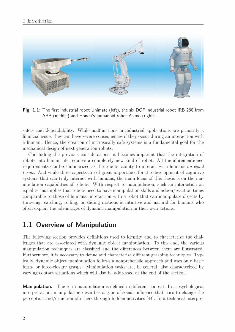
to their counterparts in industrial settings. Fig. 1.1 illustrates the evolution of robotics
over the last fifty years: the first industrial robot from Unimate, a six DOF industrial robot
from ABB, and Honda’s Asimo, which is currently one of the most advanced humanoid
robots.
For the envisioned application areas mentioned above, a high degree of autonomy con-
stitutes a characteristic feature. Tasks or plans are specified on a high-level and ultimately,
the robot should be able to decide by itself which actions to take. This is a fundamental
difference to classical industrial applications where robots typically execute predefined tra-
jectories. Additionally, the assumption of a static environment does no longer hold for the
new areas of application. The robot has to operate in changing and unknown surround-
ings. This necessitates an extensive environment perception and substantially increases
the sensor requirements. It is crucial for the robot to rely on different sensor modali-
ties and to fuse the information obtained from these sources. In addition to these sensor
skills, advanced manipulation capabilities are needed. For the physical interaction with
an unknown and changing environment, autonomous robots need a higher manipulative
dexterity than their industrial counterparts. Also, the robot is no longer stationary but is
requested to move in its environment. Such locomotion capabilities are typically realized
either through bipedal walking or through a wheeled platform. This leads to challenging
problems with respect to navigation and path planning. A number of other challenges
are related to human-robot interaction: first and foremost, in order to become a valued
partner, it is a prerequisite that the robot does not unsettle or scare the human by its
appearance. The integration of robots into human life also implies physical interaction.
Therefore, the second challenge with respect to human-robot interaction is the aspect of
1
1 Introduction
Fig. 1.1: The first industrial robot Unimate (left), the six DOF industrial robot IRB 260 fromABB (middle) and Honda’s humanoid robot Asimo (right).
safety and dependability. While malfunctions in industrial applications are primarily a
financial issue, they can have severe consequences if they occur during an interaction with
a human. Hence, the creation of intrinsically safe systems is a fundamental goal for the
mechanical design of next generation robots.
Concluding the previous considerations, it becomes apparent that the integration of
robots into human life requires a completely new kind of robot. All the aforementioned
requirements can be summarized as the robots’ ability to interact with humans on equal
terms. And while these aspects are of great importance for the development of cognitive
systems that can truly interact with humans, the main focus of this thesis is on the ma-
nipulation capabilities of robots. With respect to manipulation, such an interaction on
equal terms implies that robots need to have manipulation skills and action/reaction times
comparable to those of humans: interaction with a robot that can manipulate objects by
throwing, catching, rolling, or sliding motions is intuitive and natural for humans who
often exploit the advantages of dynamic manipulation in their own actions.
1.1 Overview of Manipulation
The following section provides definitions used to identify and to characterize the chal-
lenges that are associated with dynamic object manipulation. To this end, the various
manipulation techniques are classified and the differences between them are illustrated.
Furthermore, it is necessary to define and characterize different grasping techniques. Typ-
ically, dynamic object manipulation follows a nonprehensile approach and uses only basic
form- or force-closure grasps. Manipulation tasks are, in general, also characterized by
varying contact situations which will also be addressed at the end of the section.
Manipulation. The term manipulation is defined in different context. In a psychological
interpretation, manipulation describes a type of social influence that tries to change the
perception and/or action of others through hidden activities [44]. In a technical interpre-
2

1.1 Overview of Manipulation
tation, manipulation has a variety of meanings which all refer to physical changes in the
surrounding environment. These changes include moving one or multiple objects, joining
two or more objects by welding or gluing, or reshaping objects by cutting or grinding [88].
As pointed out by Bicchi, manipulation skills are, together with speech, probably the most
important feature that distinguish humans from animals [10].
Throughout this thesis, the term manipulation refers to the moving of objects. In
robotics, such an object manipulation is realized by robotic hands or end effectors. The
terms hand or end effector denote the interface between the robotic arm and the environ-
ment [92].
Comparing manipulation of humans and robots, Mason points out some fundamental
differences between the two [88]. One important aspect is the fact that humans possess a
larger number of (distributed) sensors and actuators. Additionally, in contrast to humans,
robots do not have the intrinsic capability to adapt to a given task. Here, human help
is needed, either by providing task instructions or by equipping the robot with learning
capabilities.
For the successful execution of a manipulation task, decisions have to be made with
respect to the explicit execution strategy. It applies to both systems, human and robotic,
that some of these decisions are made online while others are made offline, before the task
is executed. In principle, humans have a much higher intrinsic ability to make decisions
online [88]. Besides offline and online decisions, Mason differentiates a third type of decision
which he labels off-offline. Such decisions refer to the design stage of the system. Typically,
this includes the degrees of freedom, the sensor configuration, and the amount of actuation
of the robotic system.
With respect to the aforementioned decision types, the theory of manipulation distin-
guishes two challenges which are obviously coupled: the first challenge are task-related,
offline and online decisions which are needed for successful task execution. The second
challenge are decisions with respect to the mechanical design of the robotic manipulators
which are destined to perform the manipulation tasks.
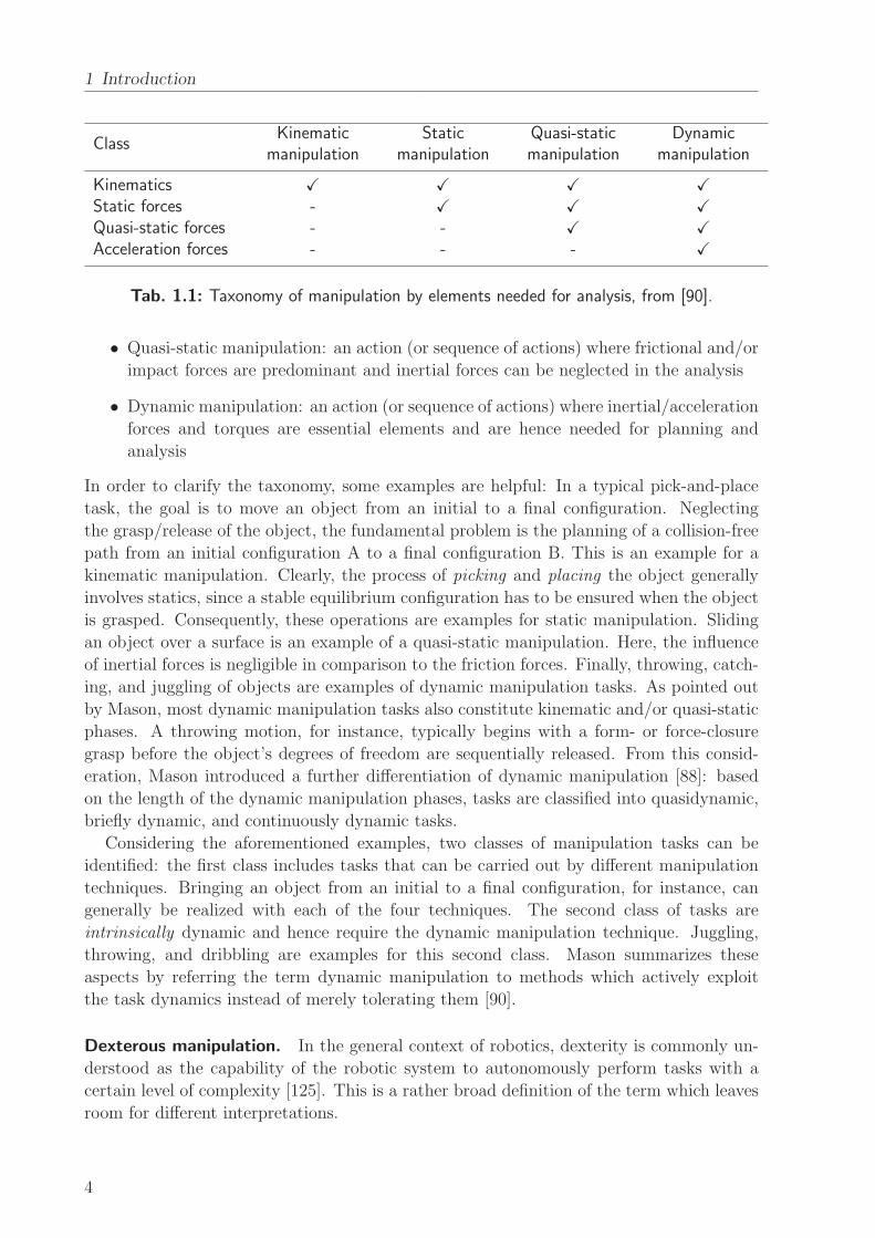
Taxonomy of manipulation techniques. The following taxonomy of manipulation is
adopted fromMason and Lynch [90]. As illustrated in Tab. 1.1, they distinguish four classes
of manipulation based on the elements which are needed for a complete description. The
classification is based on the terms kinematics, statics, and dynamics. Kinematics refers to
the motion of bodies without considering the forces/torques that cause the motion [125]. It
can be regarded as the geometry of the motion. Statics, in contrast, deals with the analysis
of forces/torques in mechanical (physical) systems that are in a static equilibrium. Finally,
dynamics is concerned with the forces/torques acting on bodies and the motions that are
related to these forces/torques. Based on the three definitions, the following manipulation
techniques can be characterized [88]:
• Kinematic manipulation: an action (or sequence of actions) which can be fully ana-
lyzed on the kinematics level
• Static manipulation: an action (or sequence of actions) where considerations with
respect to both, statics and kinematics, are needed for the analysis
3
1 Introduction
ClassKinematic
manipulationStatic
manipulationQuasi-staticmanipulation
Dynamicmanipulation
Kinematics X X X X
Static forces - X X X
Quasi-static forces - - X X
Acceleration forces - - - X
Tab. 1.1: Taxonomy of manipulation by elements needed for analysis, from [90].
• Quasi-static manipulation: an action (or sequence of actions) where frictional and/or
impact forces are predominant and inertial forces can be neglected in the analysis
• Dynamic manipulation: an action (or sequence of actions) where inertial/acceleration
forces and torques are essential elements and are hence needed for planning and
analysis
In order to clarify the taxonomy, some examples are helpful: In a typical pick-and-place
task, the goal is to move an object from an initial to a final configuration. Neglecting
the grasp/release of the object, the fundamental problem is the planning of a collision-free
path from an initial configuration A to a final configuration B. This is an example for a
kinematic manipulation. Clearly, the process of picking and placing the object generally
involves statics, since a stable equilibrium configuration has to be ensured when the object
is grasped. Consequently, these operations are examples for static manipulation. Sliding
an object over a surface is an example of a quasi-static manipulation. Here, the influence
of inertial forces is negligible in comparison to the friction forces. Finally, throwing, catch-
ing, and juggling of objects are examples of dynamic manipulation tasks. As pointed out
by Mason, most dynamic manipulation tasks also constitute kinematic and/or quasi-static
phases. A throwing motion, for instance, typically begins with a form- or force-closure
grasp before the object’s degrees of freedom are sequentially released. From this consid-
eration, Mason introduced a further differentiation of dynamic manipulation [88]: based
on the length of the dynamic manipulation phases, tasks are classified into quasidynamic,
briefly dynamic, and continuously dynamic tasks.
Considering the aforementioned examples, two classes of manipulation tasks can be
identified: the first class includes tasks that can be carried out by different manipulation
techniques. Bringing an object from an initial to a final configuration, for instance, can
generally be realized with each of the four techniques. The second class of tasks are
intrinsically dynamic and hence require the dynamic manipulation technique. Juggling,
throwing, and dribbling are examples for this second class. Mason summarizes these
aspects by referring the term dynamic manipulation to methods which actively exploit
the task dynamics instead of merely tolerating them [90].
Dexterous manipulation. In the general context of robotics, dexterity is commonly un-
derstood as the capability of the robotic system to autonomously perform tasks with a
certain level of complexity [125]. This is a rather broad definition of the term which leaves
room for different interpretations.
4
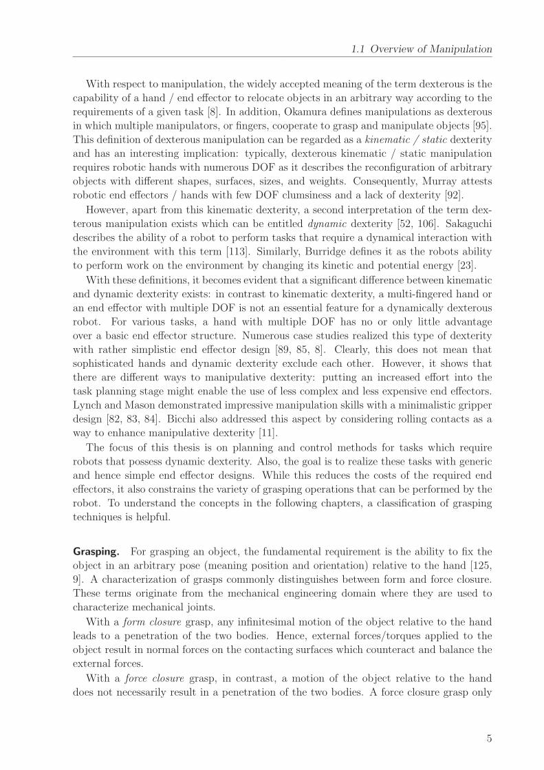
1.1 Overview of Manipulation
With respect to manipulation, the widely accepted meaning of the term dexterous is the
capability of a hand / end effector to relocate objects in an arbitrary way according to the
requirements of a given task [8]. In addition, Okamura defines manipulations as dexterous
in which multiple manipulators, or fingers, cooperate to grasp and manipulate objects [95].
This definition of dexterous manipulation can be regarded as a kinematic / static dexterity
and has an interesting implication: typically, dexterous kinematic / static manipulation
requires robotic hands with numerous DOF as it describes the reconfiguration of arbitrary
objects with different shapes, surfaces, sizes, and weights. Consequently, Murray attests
robotic end effectors / hands with few DOF clumsiness and a lack of dexterity [92].
However, apart from this kinematic dexterity, a second interpretation of the term dex-
terous manipulation exists which can be entitled dynamic dexterity [52, 106]. Sakaguchi
describes the ability of a robot to perform tasks that require a dynamical interaction with
the environment with this term [113]. Similarly, Burridge defines it as the robots ability
to perform work on the environment by changing its kinetic and potential energy [23].
With these definitions, it becomes evident that a significant difference between kinematic
and dynamic dexterity exists: in contrast to kinematic dexterity, a multi-fingered hand or
an end effector with multiple DOF is not an essential feature for a dynamically dexterous
robot. For various tasks, a hand with multiple DOF has no or only little advantage
over a basic end effector structure. Numerous case studies realized this type of dexterity
with rather simplistic end effector design [89, 85, 8]. Clearly, this does not mean that
sophisticated hands and dynamic dexterity exclude each other. However, it shows that
there are different ways to manipulative dexterity: putting an increased effort into the
task planning stage might enable the use of less complex and less expensive end effectors.
Lynch and Mason demonstrated impressive manipulation skills with a minimalistic gripper
design [82, 83, 84]. Bicchi also addressed this aspect by considering rolling contacts as a
way to enhance manipulative dexterity [11].
The focus of this thesis is on planning and control methods for tasks which require
robots that possess dynamic dexterity. Also, the goal is to realize these tasks with generic
and hence simple end effector designs. While this reduces the costs of the required end
effectors, it also constrains the variety of grasping operations that can be performed by the
robot. To understand the concepts in the following chapters, a classification of grasping
techniques is helpful.
Grasping. For grasping an object, the fundamental requirement is the ability to fix the
object in an arbitrary pose (meaning position and orientation) relative to the hand [125,
9]. A characterization of grasps commonly distinguishes between form and force closure.
These terms originate from the mechanical engineering domain where they are used to
characterize mechanical joints.
With a form closure grasp, any infinitesimal motion of the object relative to the hand
leads to a penetration of the two bodies. Hence, external forces/torques applied to the
object result in normal forces on the contacting surfaces which counteract and balance the
external forces.
With a force closure grasp, in contrast, a motion of the object relative to the hand
does not necessarily result in a penetration of the two bodies. A force closure grasp only
5

1 Introduction
requires that grasp forces exist which counteract the external forces/torques applied to the
object. Typically, this fixation of the object is realized by normal forces at the contact
points which, in turn, create friction forces.
Consequently, these definitions imply that a form closure grasp is also a force closure
grasp since it also creates forces that balance the external forces applied to the object. The
fundamental difference is that force closure allows frictional forces for the fixture of the
object. These are tangential to the contacting surfaces, whereas the counteracting forces
of a form closure grasp are normal to the contacting surfaces.
Clearly, a mixture of these grasping types is also possible and commonly referred to as
partial form closure. Here, some DOF of the object are constrained by form closure and
some by force closure.
Mason and Lynch applied their taxonomy of manipulation to grasping operations [90].
Based on the aforementioned definitions, a form closure grasp corresponds to a kinematic
grasping operation since the grasp is determined by the joint configuration of the hand. Ac-
cordingly, a force closure is equivalent to a static grasping manipulation as frictional forces
are essential for maintaining the grip. However, there are two additional manipulation
techniques that are not covered by the definitions of form and force closure: quasi-static
and dynamic manipulation. An example for the former is an end effector that pushes an
object across a surface. Here, the contact between end effector and object represents a
quasi-static grasp since the forces that maintain the contact between hand and object are
created by sliding friction. Finally, a dynamic grasp uses acceleration forces to maintain
the contact between hand and object. An example is the dribbling of a ball, where contact
is only maintained as long as the downward acceleration of the hand is larger than the
gravitational acceleration. Such a grasp is also referred to as dynamic closure.
Nonprehensile manipulation. The term nonprehensile manipulation denotes operations
that are performed without form or force closure grasps [36]. Nonprehensile manipulation
is sometimes entitled as graspless [89]. However, based on the aforementioned grasping
definitions, operations such as dynamic closures or quasi-static grasps are also nonprehen-
sile. Hence, it seems more appropriate to denote it as manipulation without form- or force
closure grasps instead of graspless manipulation. Comparing it with human manipulation,
it can be considered as just using the palm of one hand.
1.2 Applications
Exploiting dynamics in manipulation can render the object handling faster, since complex
grasping is avoided, more versatile, since robots can also cope with intrinsically dynamic
environments, and cheaper, since end effectors are generally less complex and robots can
be constructed to be less powerful. This extends the capabilities of conventional static
manipulation and opens up a new range of applications previously not feasible for robots.
In particular, the following applications can be envisioned:
• With conventional manipulation techniques, it is not possible to manipulate objects
that are oversized for conventional grippers. The paradigm of dynamic manipulation
6

1.3 Control Framework and General Approach
addresses this shortcoming: by using nonprehensile manipulation with rolling and
sliding motions, the handling of bulky objects can be realized.
• The grasping of unknown objects with a force closure grasp poses safety concerns,
e.g. if the stiffness properties of the object are not known. Hence, for manipulating
unknown objects, it is useful to employ nonprehensile techniques.
• Dynamic manipulation increases the flexibility of transportation systems and logistic
chains [37]. Manipulating objects by sliding, throwing, or catching can reduce the
transit time of such systems and, at the same time, lower the costs.
• Dynamic manipulation skills are also beneficial for autonomous robots as they in-
crease their manipulative dexterity. This, in turn, improves the handling of unfore-
seen situations, e.g. the robot can catch objects that fall from a table or out of a
cupboard that is being opened. Furthermore, dynamic manipulation skills are useful
for everyday manipulation tasks such as opening and closing doors. Here, humans
typically employ an approach that is very similar to throwing and catching of objects.
1.3 Control Framework and General Approach
In order to equip robots with dynamic manipulation skills, an extensive control framework
is needed. Such a framework poses challenges that are associated with environment percep-
tion, action planning and motion & interaction control. Fig. 1.2 depicts the overall control
structure employed in this work. It consists of four main elements: robot action planning,
dynamic force/torque observer, object tracking & trajectory prediction, and motion &
interaction control.
The robot action planning discusses how to find optimal trajectories: it proposes selec-
tion criteria and cost functions for dynamic manipulation tasks. The developed methods
Robot &
Environment
Dynamic
F/T Observer
Object
Tracking &
Trajectory
Prediction
Robot
Action
Planning
Motion &
Interaction
Control
Sec. 5.2
Ch. 3 & 4 Sec. 5.3Sec. 5.4
Control Structure
visual information
xO,(t+∆t)
xO,(t+∆t)
xM,d
xM,d
xM,d
τ
FS , MS
FE , ME
FE,d
ME,d
q
xM,a
xM,a
xM,a
Fig. 1.2: Overall control structure consisting of four main elements: robot action planning,dynamic F/T observer, object tracking & trajectory prediction, and motion & inter-action control.
7

1 Introduction
Fig. 1.3: Staubli six DOF industrial robot (left) and the dual-arm robot with 14 DOF (right).
are then applied to a number of case studies. Realizing these tasks on real hardware gener-
ally requires a perception of the environment. Here, the control framework considers visual
and force/torque sensor information: the former is used for object tracking and the latter is
used in a dynamic force/torque observer to reconstruct the interaction forces and torques.
For both modalities, the use in dynamic manipulation tasks poses additional challenges.
The type and/or the amount of feedback is chosen on a task-dependent basis. Further-
more, the execution of these tasks with real robots require precise motion and interaction
control schemes. The control framework and its aforementioned components are evaluated
in a number of experiments with the two robots depicted in Fig. 1.3.
Clearly, the hardware design is a crucial aspect for the planning and execution of dy-
namic manipulation tasks. While the mechanical design of the robotic manipulators is
not within the scope of this work, design modifications of the end effector are considered.
More specific, the thesis investigates how the use of elastic elements can enhance the robots
performance in dynamic manipulation tasks.
The planning and control methods discussed in this work rely on models of the system
and its environment. In contrast to the pursued model-based approach, learning strategies
are a way to transfer the modeling effort from the human to the robotic system [90]. Both
approaches have been successfully applied to a variety of manipulation tasks. However,
from the authors’ point of view, it is desirable to provide a task model whenever it is
possible. Furthermore, also with model-based control, the system is capable of reacting on
changing environment conditions based on adaptive control schemes.
The thesis considers the realization of dynamic manipulation tasks with generic end
effector designs. However, it is important to point out that dynamic dexterity and multi-
fingered hands do not exclude each other. On the contrary, dynamic manipulation tasks
that require hands with multiple DOF do exist, e.g. twisting a pen in one’s hand. Addi-
tionally, multi-fingered hands also fulfill other functions in addition to manipulation such
as the exploration of objects [10]. Still, most dynamic manipulation tasks can be realized
with simple end effector designs. Consequently, using such an approach is desirable as it
generalizes to more complex hands, e.g. by using only the palm of a multi-fingered hand
for a particular task.
8
1.4 Contributions and Outline of this Thesis
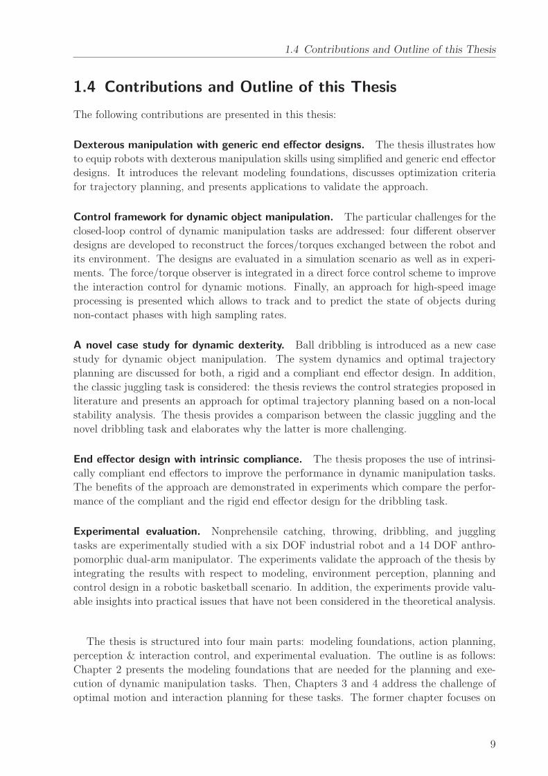
1.4 Contributions and Outline of this Thesis
The following contributions are presented in this thesis:
Dexterous manipulation with generic end effector designs. The thesis illustrates how
to equip robots with dexterous manipulation skills using simplified and generic end effector
designs. It introduces the relevant modeling foundations, discusses optimization criteria
for trajectory planning, and presents applications to validate the approach.
Control framework for dynamic object manipulation. The particular challenges for the
closed-loop control of dynamic manipulation tasks are addressed: four different observer
designs are developed to reconstruct the forces/torques exchanged between the robot and
its environment. The designs are evaluated in a simulation scenario as well as in experi-
ments. The force/torque observer is integrated in a direct force control scheme to improve
the interaction control for dynamic motions. Finally, an approach for high-speed image
processing is presented which allows to track and to predict the state of objects during
non-contact phases with high sampling rates.
A novel case study for dynamic dexterity. Ball dribbling is introduced as a new case
study for dynamic object manipulation. The system dynamics and optimal trajectory
planning are discussed for both, a rigid and a compliant end effector design. In addition,
the classic juggling task is considered: the thesis reviews the control strategies proposed in
literature and presents an approach for optimal trajectory planning based on a non-local
stability analysis. The thesis provides a comparison between the classic juggling and the
novel dribbling task and elaborates why the latter is more challenging.
End effector design with intrinsic compliance. The thesis proposes the use of intrinsi-
cally compliant end effectors to improve the performance in dynamic manipulation tasks.
The benefits of the approach are demonstrated in experiments which compare the perfor-
mance of the compliant and the rigid end effector design for the dribbling task.
Experimental evaluation. Nonprehensile catching, throwing, dribbling, and juggling
tasks are experimentally studied with a six DOF industrial robot and a 14 DOF anthro-
pomorphic dual-arm manipulator. The experiments validate the approach of the thesis by
integrating the results with respect to modeling, environment perception, planning and
control design in a robotic basketball scenario. In addition, the experiments provide valu-
able insights into practical issues that have not been considered in the theoretical analysis.
The thesis is structured into four main parts: modeling foundations, action planning,
perception & interaction control, and experimental evaluation. The outline is as follows:
Chapter 2 presents the modeling foundations that are needed for the planning and exe-
cution of dynamic manipulation tasks. Then, Chapters 3 and 4 address the challenge of
optimal motion and interaction planning for these tasks. The former chapter focuses on
9

1 Introduction
non-periodic manipulation tasks that are intrinsically dynamic, whereas the latter chapter
discusses periodic manipulation tasks with intermittent contact. Next, Chapter 5 discusses
environment perception & interaction control for dynamic manipulation tasks. Finally,
Chapter 6 presents a number of case studies in a robotic basketball scenario to evaluate
the implemented control framework in experiments.
10

2 Modeling Foundations for Dynamic Object
Manipulation
Summary The goal of this chapter is to summarize and to review state-of-the-art models
that provide the foundations for dynamic object manipulation: a hybrid system model
is introduced to capture the task dynamics with varying contact states. The contact
kinematics are outlined in a general form and it is shown how the equations simplify for
special cases such as rolling or sliding motions. In addition, the chapter discusses models
for friction and for impact events.
As detailed in Chapter 1, dynamic object manipulation extends the classical manip-
ulation techniques: besides (quasi-)static forces, it also involves acceleration forces. In
addition, the relative motion between the robotic hand and the object is actively used.
Examples for such a relative motion are rolling, sliding, spinning, and free flight phases
with no contact. Due to relative motion, impact events and friction forces are central
elements of dynamic object manipulation and must be included in the analysis. Conse-
quently, non-smooth dynamics are an important aspect in modeling. Another consequence
of the varying contact states are hybrid system dynamics. This necessitates a suitable
mathematical model to describe the hybrid control system.
The outline of the chapter is as follows: first, Section 2.1 gives some preliminary def-
initions. Next, Section 2.2 details the modeling approach for discrete-continuous control
systems that is used in this work. Then, Section 2.3 presents a classification of kinematic
constraints that occur during contact. Section 2.4 outlines a mathematical model for the
kinematics of two contacting bodies, considering different contact situations such as rolling,
sliding, spinning, and free-flight (no contact). Then, Section 2.5 discusses friction models
considering both, static and dynamic, modeling approaches. While these models are essen-
tial for task modeling, they are also important for precise robot motion control based on
inverse dynamics. Finally, Section 2.6 focuses on the modeling of impact events. Classifi-
cation criteria for impacts are outlined and two types of impact models are distinguished:
discrete (impulse-momentum) and continuous (force-based) approaches.
11

2 Modeling Foundations for Dynamic Object Manipulation
2.1 Preliminaries
The section introduces some preliminary definitions. Detailed discussions of these terms
can be found in the books by Khalil or Parker [99, 69].
Definition 2.1 (Vector field) A vector field on Rm is a smooth map which assigns a
tangent vector f(x) ∈ TqRm to each point x ∈ R
m. In local coordinates, f is expressed
as a column vector
f(x) =
f1(x)...
fm(x)
. (2.1)
Definition 2.2 (Autonomous ordinary differential equation) An n-th order au-
tonomous ordinary differential equation is defined by
x(t) = f (x(t)) (2.2)
where x(t) ∈ Rn is the system state and f : D → R
n is a locally Lipschitz vector field
(map) from domain D ⊆ Rn into R
n. A unique solution exists for every initial condition
x(t0) = x0. This solution is denoted by the flow φt(x0) which assigns a trajectory x(t) to
every initial value x0.
Generalized coordinates, configuration. A set of generalized coordinates
q(t) =
q1(t)...
qn(t)
∈ Q ⊆ R
n (2.3)
is used to describe the configuration of the system. The configuration space Q is the space
that contains all configurations of a given system.
Degrees of freedom. The degrees of freedom (DOF) of a system are defined by the
number of independent generalized coordinates.
2.2 Hybrid System Model
One of the characteristic features of dynamic object manipulation are varying contact
states. This necessitates a modeling framework for hybrid control systems. Various models
for such systems have been proposed in literature, see e.g. [144, 17, 16, 25].
The hybrid system model (HSM) used in this work has been proposed by Buss [25] and is
similar to the one developed by Branicky et al. [16]. At first sight, the model by Branicky
seems to be more general as it explicitly allows state vectors with varying dimensions.
However, this property is also implicitly included in the model by Buss, compare [25]. A
further difference between the two models exists with respect to the definition of switching
surfaces. Here, the model by Buss provides more flexibility as it allows a time dependence
12

2.2 Hybrid System Model
of the switching surfaces. The following section outlines the hybrid system model used in
this work. A detailed description of the HSM as well as a comparison with other modeling
techniques for hybrid systems can be found in [25].
The state vector of the hybrid system is defined as
ζ(t) = ζ =
[
x(t)
xd(t)
]
∈ Rn × Z (2.4)
where x(t) ∈ Rn denotes the continuous and xd(t) = 1, 2, . . . , nd ∈ Z the discrete state
of the system. Accordingly, the output of a hybrid system comprises a continuous y(t) =
h(x,u, xd, ud, t) and a discrete part yd(t) ∈ Z. The continuous control input of the hybrid
system is defined as
u(t) = u =
nd∑
k=1
δk,xduk(t) ∈ Rm (2.5)
with the Kronecker delta δk,xd being 1 if k = xd and 0 if k 6= xd. The discrete control input
is given by ud(t) ∈ Z. For a compact notation, the time dependency of the variables is
omitted in the following. With (2.4) and (2.5), the continuous dynamics are described by
vector fields of the form
f =
f 1(x,u, xd, ud, t) = f 1(x,u1, xd, ud, t) for xd = 1...
fnd(x,u, xd, ud, t) = fnd
(x,und, xd, ud, t) for xd = nd.
(2.6)
The occurrence of discrete events is defined by switching surfaces Sji
Sji : sji (x,u, xd, ud, t) = 0. (2.7)
If one of the switching conditions is fulfilled (sji (x,u, xd, ud, t) = 0), the state of the system
is reset (reinitialized) based on the transition or jump map
ζ+ =
[
x+
x+d
]
=
[
∆ji (x,ui, xd, ud, t
−)
j
]
. (2.8)
Here, t− denotes the limit from the left of time t and ζ+ = ζ(t+) is the hybrid state
immediately after the impact event (limit from the right). With (2.4)-(2.8), the definition
of a hybrid control system is complete.
Definition 2.3 (Hybrid control system) A hybrid control system is defined by its con-
tinuous dynamics
x = f i(x,ui, xd, ud, t) if sji (x,u, xd, ud, t) /∈ 0 ∀ i, j, (2.9)
transition or jump maps
ζ+ =
[
x+
x+d
]
=
[
∆ji (x,ui, xd, ud, t
−)
j
]
if sji (x,u, xd, ud, t−) = 0, (2.10)
and outputs y(t) = h(x,u, xd, ud, t) and yd(t).
13
2 Modeling Foundations for Dynamic Object Manipulation
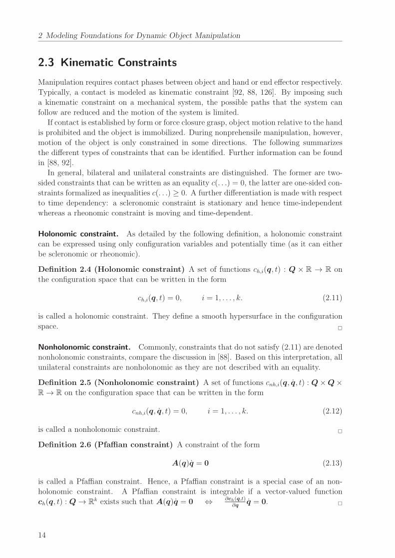
2.3 Kinematic Constraints
Manipulation requires contact phases between object and hand or end effector respectively.
Typically, a contact is modeled as kinematic constraint [92, 88, 126]. By imposing such
a kinematic constraint on a mechanical system, the possible paths that the system can
follow are reduced and the motion of the system is limited.
If contact is established by form or force closure grasp, object motion relative to the hand
is prohibited and the object is immobilized. During nonprehensile manipulation, however,
motion of the object is only constrained in some directions. The following summarizes
the different types of constraints that can be identified. Further information can be found
in [88, 92].
In general, bilateral and unilateral constraints are distinguished. The former are two-
sided constraints that can be written as an equality c(. . .) = 0, the latter are one-sided con-
straints formalized as inequalities c(. . .) ≥ 0. A further differentiation is made with respect
to time dependency: a scleronomic constraint is stationary and hence time-independent
whereas a rheonomic constraint is moving and time-dependent.
Holonomic constraint. As detailed by the following definition, a holonomic constraint
can be expressed using only configuration variables and potentially time (as it can either
be scleronomic or rheonomic).
Definition 2.4 (Holonomic constraint) A set of functions ch,i(q, t) : Q × R → R on
the configuration space that can be written in the form
ch,i(q, t) = 0, i = 1, . . . , k. (2.11)
is called a holonomic constraint. They define a smooth hypersurface in the configuration
space.
Nonholonomic constraint. Commonly, constraints that do not satisfy (2.11) are denoted
nonholonomic constraints, compare the discussion in [88]. Based on this interpretation, all
unilateral constraints are nonholonomic as they are not described with an equality.
Definition 2.5 (Nonholonomic constraint) A set of functions cnh,i(q, q, t) : Q×Q×
R → R on the configuration space that can be written in the form
cnh,i(q, q, t) = 0, i = 1, . . . , k. (2.12)
is called a nonholonomic constraint.
Definition 2.6 (Pfaffian constraint) A constraint of the form
A(q)q = 0 (2.13)
is called a Pfaffian constraint. Hence, a Pfaffian constraint is a special case of an non-
holonomic constraint. A Pfaffian constraint is integrable if a vector-valued function
ch(q, t) : Q → Rk exists such that A(q)q = 0 ⇔ ∂ch(q,t)
∂qq = 0.
14

2.4 Contact Kinematics
From this definition it follows that an integrable Pfaffian constraint is equivalent to a
holonomic constraint [92].
Virtual holonomic constraint. Typically, the restrictions described by a holonomic
constraint are physically imposed on the system. However, it is also possible to define
artificial or virtual geometric constraints for a given system [123, 143]. In contrast to
a holonomic constraint, these virtual holonomic constraints have to be fulfilled by some
control action. As detailed in Chapter 4, such constraints can be used for the control of
underactuated periodic manipulation tasks.
2.4 Contact Kinematics
Contact modeling is a fundamental aspect in the planning of robotic tasks. This includes
robotic walking machines, robotic hands grasping objects, and part handling in industrial
scenarios [86]. The following section considers contact kinematics from a manipulation
perspective and outlines the model originally developed by Montana [91].
Assumptions. The derivation of the kinematic contact equations is based on the following
assumptions:
A1 Contacts can be regarded as point contacts.
A2 For two bodies, contact occurs only at one point.
A3 The surfaces of the contacting bodies are regular.
Surface parameterization. Given an object in R3 with an arbitrary regular surface S,
this surface can be locally described by the orthogonal parameterization c : R2 → R3,
c(u, v) =
f1(u, v)
f2(u, v)
f3(u, v)
. (2.14)
Tangent plane. The tangent plane to the surface is spanned by the vectors
cu(u, v) :=∂c
∂ucv(u, v) :=
∂c
∂v. (2.15)
Kinematic equations of contact. In the following, the subscripts 1 and 2 denote the
two bodies. A schematic of a general contact situation is depicted in Fig. 2.1. The surfaces
of the two bodies in the body-fixed coordinate frames Σ1, Σ2 are parameterized according
to (2.14). The contact frames Σc1, Σc2 are defined as the normalized Gauss frames at the
contact point. The angle ψ is defined as the rotation angle around the z-axis of Σc2 that
aligns the x-axes of Σc1 and Σc2. Additionally, the body-fixed frames Σl1(t), Σl2(t) are
defined that coincide with the respective contact frame at time t. The motion of object 1
15

2 Modeling Foundations for Dynamic Object Manipulation
Body 1
Body 2
Σ1
Σ2
Σc2Σc1
ψ
cu,1
cv,1
n1
cu,2
cv,2
n2
Fig. 2.1: Motion of two bodies in contact, adopted from [92].
relative to object 2 is then described by the translational v =[
vx vy vz]T
and rotational
ω =[
ωx ωy ωz]T
velocity of Σl1(t) relative to Σl2(t). The contact kinematics are given
by [91]
[
u1v1
]
= M−11
(
K1 + K2
)−1([
−ωyωx
]
− K2
[
vxvy
])
,
[
u2v2
]
= M−12 Rψ
(
K1 + K2
)−1([
−ωyωx
]
+K1
[
vxvy
])
, (2.16)
ψ = ωz + T 1M 1
[
u1v1
]
+ T 2M 2
[
u2v2
]
,
0 = vz.
with K2 = RψK2Rψ and Rψ =
[
cosψ − sinψ
− sinψ − cosψ
]
.
Here, M is the metric tensor, K is the curvature tensor, and T is the torsion form of the
corresponding surface. The three quantities are commonly referred to as the geometric
parameters of a surface. Details on these terms can be found in the book by Murray [92]
and in Appendix A.1.
The equations (2.16) describe the kinematics of a point contact in its most general form.
Special types of relative motion are realized by imposing additional constraints - this is
detailed in the following subsections.
2.4.1 Sliding
A sliding motion imposes the constraint of zero rotational velocity,
ωx = ωy = ωz = 0. (2.17)
2.4.2 Rolling
Here, rolling and pure rolling are distinguished. For the former, the following conditions
vx = vy = 0, (2.18)
16
2.5 Friction
have to be fulfilled. Pure rolling adds the constraint of no spin motion,
vx = vy = ωz = 0. (2.19)
2.4.3 Spinning
A spinning motion comprises only rotational velocities in normal direction to the tangential
contact plane,
ωx = ωy = vx = vy = 0. (2.20)
2.4.4 No Contact / Free-Flight
Finally, the special case of no contact between object and end effector is considered. Here,
none of the objects’ six DOF is constrained and nonzero velocities vz are allowed [88]. The
motion of the object is determined by gravitational acceleration and possibly air resistance.
2.5 Friction
Friction is a nonlinear phenomenon which is of great importance for various engineering
disciplines. With respect to this work, there are three reasons for the interest in accurate
friction models: first, nonprehensile manipulation includes relative motion between object
and hand such as rolling or sliding. Hence, to plan these tasks, a model of the friction forces
is essential. The second reason is related to the motion control of robotic manipulators.
The successful execution of dynamic manipulation tasks with robotic systems requires a
precise motion control of the robot. This is typically achieved by an inverse dynamics
scheme which necessitates an accurate description of the friction forces as part of the
dynamic model, see Sec. 5.3 for details. Finally, friction is an important aspect when
considering impact between bodies with nonsmooth surfaces.
Numerous friction models have been proposed. Detailed surveys on these models can
be found in [4, 97]. In general, one distinguishes static and dynamic friction models.
The characteristic feature of static models is that the friction force only depends on the
current velocity. Hence, non-stationary friction phenomena such as micro-slip or hysteretic
behavior are not captured by static models. This shortcoming is addressed by dynamic
(or state variable) friction models. These models introduce one (or more) state variable(s)
and the friction force is a function of the current velocity and the state variable(s). In the
following, static and dynamic friction models are briefly discussed and their suitability for
the different purposes (trajectory planning, impact modeling, and friction compensation
in motion control) is evaluated.
2.5.1 Static Models
This category includes all models that use static maps between velocity and friction
force [27]. Classical static friction models comprise a combination of four components,
which capture the fundamental friction phenomena.
17
2 Modeling Foundations for Dynamic Object Manipulation
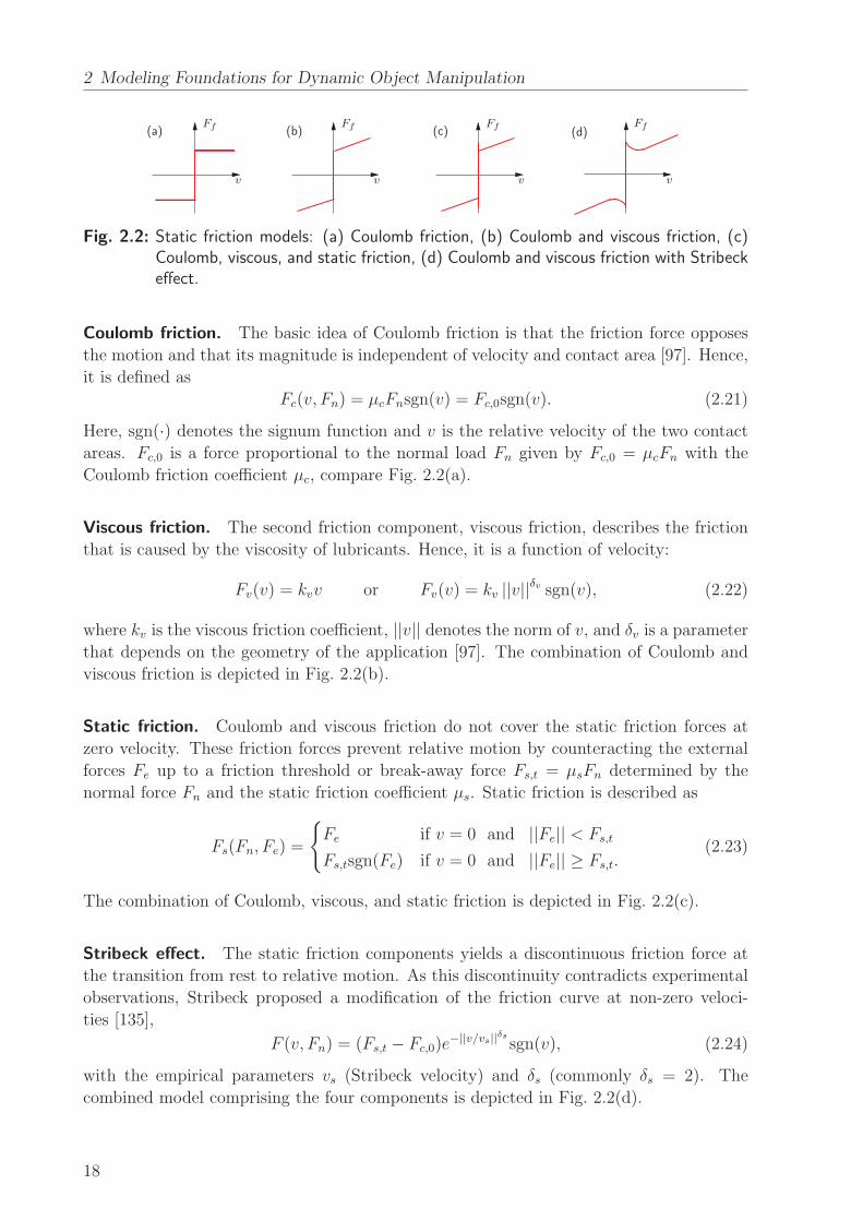
(a) (b) (c) (d)FfFfFfFf
vvvv
Fig. 2.2: Static friction models: (a) Coulomb friction, (b) Coulomb and viscous friction, (c)Coulomb, viscous, and static friction, (d) Coulomb and viscous friction with Stribeckeffect.
Coulomb friction. The basic idea of Coulomb friction is that the friction force opposes
the motion and that its magnitude is independent of velocity and contact area [97]. Hence,
it is defined as
Fc(v, Fn) = µcFnsgn(v) = Fc,0sgn(v). (2.21)
Here, sgn(·) denotes the signum function and v is the relative velocity of the two contact
areas. Fc,0 is a force proportional to the normal load Fn given by Fc,0 = µcFn with the
Coulomb friction coefficient µc, compare Fig. 2.2(a).
Viscous friction. The second friction component, viscous friction, describes the friction
that is caused by the viscosity of lubricants. Hence, it is a function of velocity:
Fv(v) = kvv or Fv(v) = kv ||v||δv sgn(v), (2.22)
where kv is the viscous friction coefficient, ||v|| denotes the norm of v, and δv is a parameter
that depends on the geometry of the application [97]. The combination of Coulomb and
viscous friction is depicted in Fig. 2.2(b).
Static friction. Coulomb and viscous friction do not cover the static friction forces at
zero velocity. These friction forces prevent relative motion by counteracting the external
forces Fe up to a friction threshold or break-away force Fs,t = µsFn determined by the
normal force Fn and the static friction coefficient µs. Static friction is described as
Fs(Fn, Fe) =
Fe if v = 0 and ||Fe|| < Fs,t
Fs,tsgn(Fe) if v = 0 and ||Fe|| ≥ Fs,t.(2.23)
The combination of Coulomb, viscous, and static friction is depicted in Fig. 2.2(c).
Stribeck effect. The static friction components yields a discontinuous friction force at
the transition from rest to relative motion. As this discontinuity contradicts experimental
observations, Stribeck proposed a modification of the friction curve at non-zero veloci-
ties [135],
F (v, Fn) = (Fs,t − Fc,0)e−||v/vs||
δs
sgn(v), (2.24)
with the empirical parameters vs (Stribeck velocity) and δs (commonly δs = 2). The
combined model comprising the four components is depicted in Fig. 2.2(d).
18
2.5 Friction
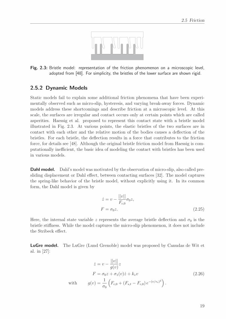
Fig. 2.3: Bristle model: representation of the friction phenomenon on a microscopic level,adopted from [48]. For simplicity, the bristles of the lower surface are shown rigid.
2.5.2 Dynamic Models
Static models fail to explain some additional friction phenomena that have been experi-
mentally observed such as micro-slip, hysteresis, and varying break-away forces. Dynamic
models address these shortcomings and describe friction at a microscopic level. At this
scale, the surfaces are irregular and contact occurs only at certain points which are called
asperities. Haessig et al. proposed to represent this contact state with a bristle model
illustrated in Fig. 2.3. At various points, the elastic bristles of the two surfaces are in
contact with each other and the relative motion of the bodies causes a deflection of the
bristles. For each bristle, the deflection results in a force that contributes to the friction
force, for details see [48]. Although the original bristle friction model from Haessig is com-
putationally inefficient, the basic idea of modeling the contact with bristles has been used
in various models.
Dahl model. Dahl’s model was motivated by the observation of micro-slip, also called pre-
sliding displacement or Dahl effect, between contacting surfaces [32]. The model captures
the spring-like behavior of the bristle model, without explicitly using it. In its common
form, the Dahl model is given by
z = v −||v||
Fc,0σ0z,
F = σ0z. (2.25)
Here, the internal state variable z represents the average bristle deflection and σ0 is the
bristle stiffness. While the model captures the micro-slip phenomenon, it does not include
the Stribeck effect.
LuGre model. The LuGre (Lund Grenoble) model was proposed by Canudas de Wit et
al. in [27]:
z = v −||v||
g(v)z
F = σ0z + σ1(v)z + kvv (2.26)
with g(v) =1
σ0
(
Fc,0 + (Fs,t − Fc,0) e−(v/vs)2
)
.
19

2 Modeling Foundations for Dynamic Object Manipulation
Again, the variables z and σ0 denote the average bristle deflection and stiffness, σ1(v) is
the damping, and g(v) captures Coulomb friction and Stribeck effect. When g(v) = Fc/σ0and σ1 = kv = 0, the LuGre model reduces to the Dahl model. The central advantages
of the LuGre model are its completeness with respect to the modeled friction phenomena
and the relatively low number of parameters. In total, six parameters have to be identified
for the LuGre model: the ones already known from the static models (Fc,0, Fs,t, kv, vs)
and the two additional parameters σ0 and σ1.
Beside these two, other dynamic friction models have been proposed: Bliman and Sorine
presented an extension of Dahl’s model using two state variables [13]. However, their
model does neither capture the Stribeck effect nor frictional lag [40]. Armstrong-Helouvry
introduced a dynamic friction model with seven parameters. This model includes the
various friction phenomena by using different models for stiction and sliding [4].
2.6 Impacts
For interacting bodies, impacts are an essential phenomenon: they occur when two ore more
bodies collide with each other and are characterized by a short time duration and high
force levels. For various research areas, such impact events are of great relevance. Popular
examples are walking/hopping machines or drive trains with backlash. Impacts are also an
important element in dynamic manipulation. To this end, the section characterizes impact
types and reviews the state-of-the-art models to describe them. The aim of these models
is to determine/predict the post-impact state of the system based on its pre-impact state.
Clearly, the modeling process depends on the intended usage of the model: an online usage
imposes constraints on the model complexity and hence reduces the accuracy.
The following subsections discuss the impact events that are relevant for dynamic object
manipulation, namely collisions between two bodies with a single contact point. A general
introduction to non-smooth dynamics can be found in the book by Brogliato [18]. An
extensive literature survey on the modeling of impact dynamics was provided by Gilardi
and Sharf [45].
2.6.1 Classification Criteria
When an impact event occurs, the two colliding bodies get in contact. The case of a general
impact between two bodies is illustrated in Fig. 2.4. The line of impact is the common
normal on the contacting surfaces. In the following, velocities along the line of impact are
denoted as normal velocities with subscript n. Accordingly, velocities in the tangential
plane of the contact are labeled with the subscript t.
Independent of the model that is used for the mathematical description, impacts are
classified based on the following criteria [45].
Direct and oblique impact. As depicted in Fig. 2.5(a), an impact is denoted as direct if
the pre-impact velocities of the two bodies are along the line of impact. Accordingly, an
oblique impact occurs if one or both initial velocities do not fulfill this condition, compare
Fig. 2.5(b). In the latter case, at least one body has a non-zero tangential velocity.
20

2.6 Impacts
Tangential plane
t1
t2
n
Fig. 2.4: Illustration of a general impact between two bodies.
(a) (b) (c) (d)
COG 1
COG 1 COG 2COG 2
v1v1v2
v2
tttt
nnnn
Fig. 2.5: Classification of impacts: (a) direct, (b) oblique, (c) central / collinear, (d) eccentric.
Central and eccentric impact. An impact is characterized as central or collinear if the
centers of mass are on the line of impact, see Fig. 2.5(c). Consequently, the impact forces
in normal direction do not change the rotational velocity. In contrast, for an eccentric
impact the center of mass of one or both bodies is not on the line of impact, compare
Fig. 2.5(d). Hence, the rotational velocity after the impact is changed due to the impact
forces in normal direction.
Energy loss. For all impact events, a compression and a restitution phase can be distin-
guished. The compression phase begins with the initial contact of the two bodies. The
transition to the restitution phase occurs at the time of maximum deformation when the
relative velocity between the two bodies is zero. The end of the restitution phase is reached
when the bodies separate.
Depending on the energy loss during the impact event, four impact types are character-
ized: a perfectly elastic impact occurs when no kinetic energy is lost during the collision
and the deformation is completely reversed. In contrast, for a perfectly inelastic or plastic
collision, the maximum possible amount of kinetic energy is lost, the two bodies deform
and stick together after the impact. If the kinetic energy is not completely conserved but
the deformation is completely reversed, the impact is partially elastic. Finally, an impact
with a partial loss of kinetic energy and some amount of permanent deformation is denoted
as partially plastic.
21
2 Modeling Foundations for Dynamic Object Manipulation
The first two types are idealized cases: a perfectly elastic impact assumes that the energy
flow from the initial kinetic energy to the elastic strain energy is completely reversible.
Similarly, a perfectly inelastic collision assumes that the lost kinetic energy is completely
transferred into plastic deformation. In reality, impacts of two colliding masses are partially
plastic or partially elastic and hence a mixture of the idealized cases. Typically, not all
of the initial kinetic energy is transformed into elastic strain or plastic deformation: some
energy is dissipated in other processes such as wave propagation, sound, and heat [45].
Smooth and frictional impact. Friction is an important aspect as it can stop or reverse
the tangential motion during an impact. In contrast, if the impact is assumed frictionless,
no tangential forces can be exchanged between the two bodies and the impulse in tangential
direction, ∆Pt is zero.
2.6.2 Discrete Models
Discrete or impulse-momentum-based impact models are based on the following assump-
tions: the impact event is instantaneous and the occurring impact forces are impulsive.
This implies discontinuous changes in the velocities of the colliding bodies while the posi-
tions are invariant. In addition, forces that are not caused by the impact (e.g. gravitational
or spring forces) are assumed to be negligible. Typically, discrete models are used for the
collision of bodies that can be considered as effectively rigid [45, 145]. This criteria is
fulfilled if strain energy is negligible and the contact area is small compared to the size of
the body [136]. Discrete models are based on the specification of a coefficient of restitution
(COR) cr, which describes the plasticity of the impact and varies in the range from 0 (per-
fectly plastic) to 1 (perfectly elastic). The aforementioned assumption of an instantaneous
impact with discontinuous changes in the velocities results in infinitely large impact forces.
Hence, it is more suitable to deal with impulses instead. In the following, the subscript
specifies the body (1 or 2) and the superscript + denotes post-impact velocities.
The change in momentum over a time interval [ti, tf ] or the so called impulse-momentum
equations are given by
∆P = m∆v = m(vf − vi) =
∫ tf
ti
F dt,
∆L = J∆ω = J(ωf − ωi) =
∫ tf
ti
Mdt =
∫ tf
ti
r × F dt, (2.27)
where P / L denotes the linear / angular momentum, m and J are the mass and the
inertia tensor of the body, and r is the vector from the center of mass to the contact point.
With conservation of momentum, the sum of momentum of two bodies before and after a
collision is equal
m1v1 +m2v2 = m1v+1 +m2v
+2 , (2.28)
J1ω1 + J2ω2 = J1ω+1 + J2ω
+2 . (2.29)
Discrete models decouple the impact problem into a contact problem in normal direction
22
2.6 Impacts
and a friction problem in tangential direction [46]: the linear impulse ∆P is divided in a
normal impulse ∆Pn and a tangential impulse ∆Pt. Accordingly, the relative translational
velocity at the contact point C is divided into a normal component vC,n and a tangential
component vC,t.
Normal direction. In normal direction, the most common models are the impact laws by
Poisson, Newton, and Stronge.
• Poisson’s COR. The normal impulse ∆Pn of an impact is the sum of the impulses
in the compression and restitution phase
∆Pn = ∆Pn,c +∆Pn,r. (2.30)
In Poisson’s hypothesis, the coefficient of restitution is defined as the ratio of the
compression and the restitution impulse
cr,P =∆Pn,c∆Pn,r
. (2.31)
• Newton’s COR. While Poisson’s COR is based on the impulses during impact,
Newton’s model determines the coefficient of restitution based on velocities. Let vC,n(v+C,n) denote the relative normal velocity of the contact point C before (after) the
impact. Then, Newton’s model defines the coefficient of restitution as
cr,N = −v+C,nvC,n
. (2.32)
• Stronge’s COR. Stronge’s model defines the COR as ratio of the work W in resti-
tution (subscript r) and compression phase (subscript c) [136],
cr,S = −Wr
Wc
. (2.33)
Tangential direction. The aforementioned three coefficients are for the normal direction.
However, if the contacting surfaces are not smooth, changes in the translational velocities
tangential to the impact plane and the rotational velocities will be induced [45]. A common
method to reflect these changes is related to Newton’s COR and specifies coefficients of
restitution for these directions as
cr,t = −v+C,tvC,t
cr,r = −ω+C
ωC. (2.34)
Brach proposesd an alternative approach and related the tangential and normal im-
pulse [15],
∆Pt = µ∆Pn. (2.35)
For collinear or smooth (non-frictional) impacts, the models of Poisson, Newton, and
Stronge are equivalent. However, for frictional impacts with transitions from slip to stick
23

2 Modeling Foundations for Dynamic Object Manipulation
or slip-reversal, Newton’s and Poisson’s model can lead to different energetic inconsisten-
cies [136]. Despite this shortcoming, velocity-based coefficients of restitution will be used
in this work as they provide an accurate description for central impacts of effectively rigid
bodies and as their mathematical compactness allows a direct integration into the task
planning.
2.6.3 Continuous Models
Continuous or force-based impact models relax the assumptions of the discrete models:
they consider a finite impact duration and the positions of the colliding bodies are not
fixed during impact. As the deformation of the objects is explicitly taken into account,
continuous models are particularly well suited for the impact of elastic bodies [76]. Various
continuous models have been proposed to capture the deformation and energy loss during
impact, e.g. the models of Hertz, Kelvin-Voigt, and Hunt-Crossley [50, 58]. Commonly,
continuous models include (possibly nonlinear) spring and damper forces. in the following
paragraph, this is exemplarily illustrated for the Hunt-Crossley model.
Hunt-Crossley model. For this model, the impact force in normal direction consists of
a nonlinear spring and a nonlinear damping force
F (t) = −ksxλ1 − kdx
λ2 x. (2.36)
where x is the penetration, x the penetration velocity, ks the spring constant, and kd the
damper constant [58]. The exponents λ1, λ2 take into account the geometry of the contact
and in its common form, λ = λ1 = λ2 takes a value close to one. Methods for the parameter
identification of continuous models have been proposed in [7, 47, 33].
2.6.4 Extensions
Multibody systems. The previous models considered the collision of two bodies at a sin-
gle contact point. Impact situations for multi-body systems and/or with multiple contacts
were addressed by Glocker and Pfeiffer [46, 100]. Studer investigated such systems of rigid
bodies with non-smooth dynamics and developed a simulation environment [137].
Elastic bodies. Discrete and continuous model are both based on lumped parameters.
For elastic bodies, distributed models can be used to describe the deformation and the
energy loss during impacts. The Bullet physics project is one of the few examples that
considers soft body dynamics [30]. Tian and Jia presented a distributed model for the
specific class of deformable, shell-like objects [138].
2.7 Summary
This chapter provided the modeling foundations for dynamic object manipulation. To
this end, state-of-the-art models for the relevant areas were outlined and briefly discussed.
24

2.7 Summary
Section 2.2 introduced a hybrid system model to cover the discrete and continuous aspects
that are characteristic for dynamic manipulation tasks. Section 2.3 discussed the different
types of kinematic constraints that occur during contact. Then, in Section 2.4, the kine-
matic equations for two contacting surfaces were derived. Next, Section 2.5 outlined the
fundamental properties of static and dynamic friction models. For the planning of manip-
ulation tasks, the static models provide sufficient accuracy. For friction compensation in
robotic motion control schemes, however, dynamic models are generally preferable. Here,
the LuGre model offers the best trade-off between accuracy and mathematical complexity.
Finally, Section 2.6 considered the modeling of impact events. Both, discrete and con-
tinuous, impact models were outlined. The former are based on the impulse-momentum
equations and assume an instantaneous impact. The mathematical compactness of discrete
models comes at the cost of reduced accuracy and potential inconsistencies for frictional
impacts. In contrast, the continuous models consider a finite impact duration and motion
of the objects during impact. Naturally, this results in an increased mathematical com-
plexity. As the manipulated objects in this work are considered to be effectively rigid,
the discrete models provide an accurate description. For manipulation tasks with elastic
bodies, continuous or distributed impact models are preferable.
25

2 Modeling Foundations for Dynamic Object Manipulation
26

3 Non-Periodic Dynamic Manipulation Tasks
Summary This chapter discusses non-periodic dynamic manipulation tasks and details
how dynamic dexterity can be realized with generic end effector designs. The planning of
optimal trajectories is addressed: the chapter summarizes the constraints that have to be
considered and discusses criteria for the trajectory optimization. Three exemplary appli-
cations are studied: first, rolling manipulation is considered with a ball-on-plate system.
Second, dual-handed ball throwing using a basic force closure grasp is addressed. Third,
a nonprehensile approach for robotic catching is presented and two catching strategies are
discussed.
While there are animals with locomotion or sensor capabilities superior to those of
humans, the dexterous manipulation skills of humans are outstanding [10]. This is due to
two reasons: superior grasping capabilities and a better coordination between sensor and
motor skills. For conventional dexterous manipulation, advanced grasping capabilities are
a prerequisite. This is illustrated by the fact that a general form closure grasp requires
seven contact points [125]. Hence, multi-fingered hands are needed to manipulate objects of
different size and shape with a form closure grasp. For dynamical dexterous manipulation,
the grasping capabilities are less important. Many dynamic manipulation tasks can be
performed in a nonprehensile fashion using only a single contact point between end effector
and object [57, 84]. Instead, these tasks require a high ability of coordination between
sensor and motor skills.
In general, the successful execution of manipulation tasks requires task-specific decisions.
Some of these decisions can be made offline while others have to be made online during the
task execution. Offline decisions commonly include a preselection that specifies the overall
strategy for a particular task. Online decisions include the compensation of disturbances
or the reaction to unforeseen events. The planning approach pursued in this work includes
both decision types: first, a number of selection criteria are evaluated offline. The creation
of look-up tables then allows to evaluate these selection criteria online and create the
corresponding trajectory.
The outline of the chapter is as follows: first, Section 3.1 provides an overview of
related work. In Section 3.2, the planning of motion and force trajectories for these tasks
is addressed. Then, Section 3.3 presents applications for rigid end effector designs.
27

3 Non-Periodic Dynamic Manipulation Tasks
3.1 Related Work
Robots with dynamic skills have been studied in various research works: Hodgins and
Raibert were among the first and investigated dynamic locomotion primitives such as hop-
ping for robots [52]. With respect to manipulation, dynamic dexterity was first addressed
by Mason and Lynch [90]. Their work was motivated by the following considerations: first,
dynamic manipulation is either the most efficient or even the only method to perform cer-
tain tasks. Second, dynamic dexterity helps to reduce the complexity of the end effector
and/or manipulator. Third, exploiting the task dynamics by following a graspless (non-
prehensile) approach is beneficial for the handling of bulky objects. The new manipulation
paradigm was demonstrated for tasks such as planar throwing or snatching using mini-
malistic robots and open-loop control [82, 84]. Dynamical dexterous manipulation skills
for different robots were also discussed by Koditschek et al. [71]. In addition to motion
planning, they addressed closed-loop control of these tasks based on visual feedback [106].
Huang investigated impulsive manipulation as an example of dynamic manipulation with
intermittent contact [57]. In his work, the action planning was decomposed into an inverse
sliding problem, which determined the required velocities to drive an object to the desired
state, and an impact problem, which determined the parameters of the collision between
object and actuator. The presented case studies were restricted to planar problems.
Robotic throwing tasks were investigated by several researchers: Kato and co-workers
planned throwing motions and presented experimental results for a two DOF robot and
an object with mass 0.01 kg [67]. Katsumata et al. discussed a throwing task with an
underactuated two DOF robotic manipulator [68]. Considering more complex robotic
structures, Lombai and Szederkenyi followed an offline approach to optimize throwing
trajectories for a six DOF robot [79]. Senoo used a four DOF manipulator and a robotic
hand to generate throwing trajectories for a tennis ball [120]. They proposed a rolling
motion of the ball on the hand in order to increase the release velocity.
The task of robotic ball catching has also been studied by various researchers: Andersson
realized two-dimensional catching of ping-pong balls with a robotic arm [3]. Hove and
Slotine presented spatial catching with a four DOF manipulator [55]. Burridge et al.
described a mirror law for catching a ball with a three DOF robot and a planar paddle
end effector [24, 23]. Frese et al. presented ball catching with a seven DOF robot [38].
In their setup, a basket served as end effector to catch the ball. Bauml et al. discussed
kinematically optimal catching with a seven DOF robot and a robotic hand [6]. Riley
and Atkeson investigated ball catching with a humanoid robot using a baseball glove to
catch [103]. Frank et al. considered shooting and catching as a new technology within
logistic chains [37]. In a first experimental study, a Gantry type robot was used to catch
objects with up to 0.06 kg.
The large majority of the aforementioned work is based on strategies that applied a form-
or force-closure grasp to catch/throw the object. Additionally, the mass of the manipulated
object was sufficiently small and thus neglected. In contrast to these approaches, this
chapter considers the skill of nonprehensile catching. Such a skill is beneficial as it allows
to catch objects that are too large for conventional robotic hands. Furthermore, the chapter
discusses catching and throwing of objects with non-negligible mass properties.
28
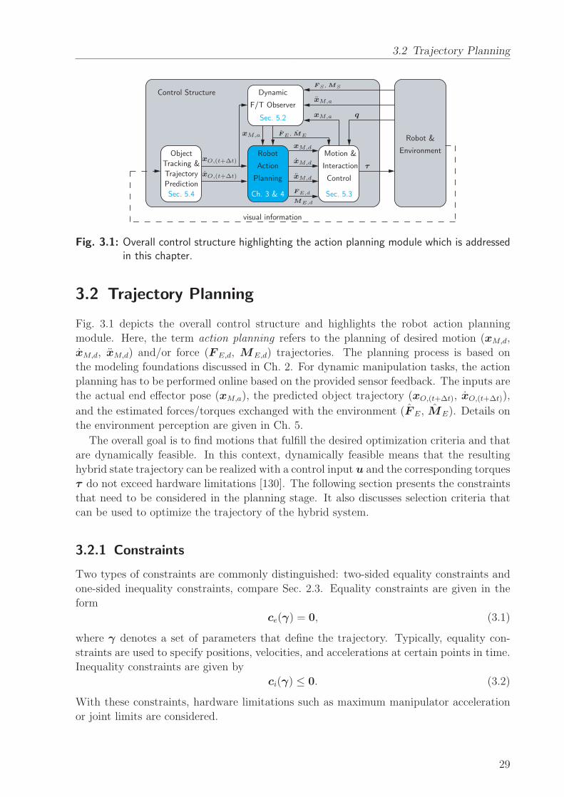
3.2 Trajectory Planning
Robot &
Environment
Dynamic
F/T Observer
Object
Tracking &
Trajectory
Prediction
Robot
Action
Planning
Motion &
Interaction
Control
Sec. 5.2
Ch. 3 & 4 Sec. 5.3Sec. 5.4
Control Structure
visual information
xO,(t+∆t)
xO,(t+∆t)
xM,d
xM,d
xM,d
τ
FS , MS
FE , ME
FE,d
ME,d
q
xM,a
xM,a
xM,a
Fig. 3.1: Overall control structure highlighting the action planning module which is addressedin this chapter.
3.2 Trajectory Planning
Fig. 3.1 depicts the overall control structure and highlights the robot action planning
module. Here, the term action planning refers to the planning of desired motion (xM,d,
xM,d, xM,d) and/or force (F E,d, ME,d) trajectories. The planning process is based on
the modeling foundations discussed in Ch. 2. For dynamic manipulation tasks, the action
planning has to be performed online based on the provided sensor feedback. The inputs are
the actual end effector pose (xM,a), the predicted object trajectory (xO,(t+∆t), xO,(t+∆t)),
and the estimated forces/torques exchanged with the environment (F E, ME). Details on
the environment perception are given in Ch. 5.
The overall goal is to find motions that fulfill the desired optimization criteria and that
are dynamically feasible. In this context, dynamically feasible means that the resulting
hybrid state trajectory can be realized with a control input u and the corresponding torques
τ do not exceed hardware limitations [130]. The following section presents the constraints
that need to be considered in the planning stage. It also discusses selection criteria that
can be used to optimize the trajectory of the hybrid system.
3.2.1 Constraints
Two types of constraints are commonly distinguished: two-sided equality constraints and
one-sided inequality constraints, compare Sec. 2.3. Equality constraints are given in the
form
ce(γ) = 0, (3.1)
where γ denotes a set of parameters that define the trajectory. Typically, equality con-
straints are used to specify positions, velocities, and accelerations at certain points in time.
Inequality constraints are given by
ci(γ) ≤ 0. (3.2)
With these constraints, hardware limitations such as maximum manipulator acceleration
or joint limits are considered.
29
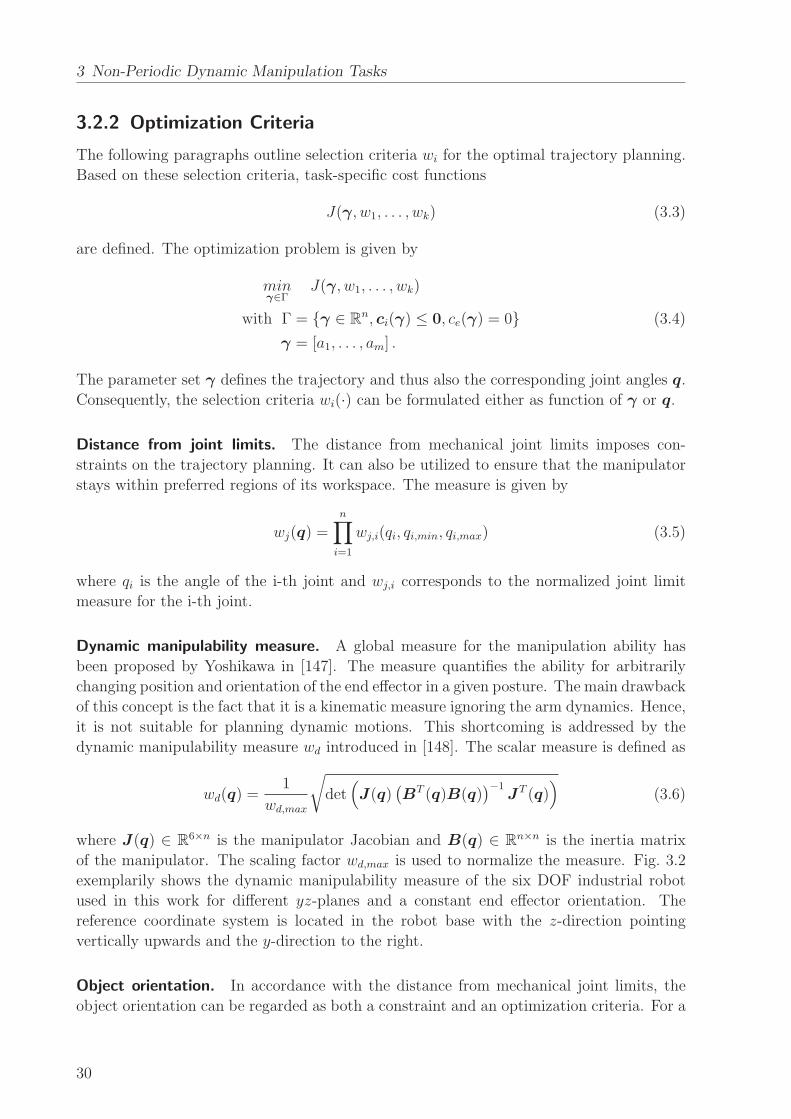
3 Non-Periodic Dynamic Manipulation Tasks
3.2.2 Optimization Criteria
The following paragraphs outline selection criteria wi for the optimal trajectory planning.
Based on these selection criteria, task-specific cost functions
J(γ, w1, . . . , wk) (3.3)
are defined. The optimization problem is given by
minγ∈Γ
J(γ, w1, . . . , wk)
with Γ = γ ∈ Rn, ci(γ) ≤ 0, ce(γ) = 0 (3.4)
γ = [a1, . . . , am] .
The parameter set γ defines the trajectory and thus also the corresponding joint angles q.
Consequently, the selection criteria wi(·) can be formulated either as function of γ or q.
Distance from joint limits. The distance from mechanical joint limits imposes con-
straints on the trajectory planning. It can also be utilized to ensure that the manipulator
stays within preferred regions of its workspace. The measure is given by
wj(q) =n∏
i=1
wj,i(qi, qi,min, qi,max) (3.5)
where qi is the angle of the i-th joint and wj,i corresponds to the normalized joint limit
measure for the i-th joint.
Dynamic manipulability measure. A global measure for the manipulation ability has
been proposed by Yoshikawa in [147]. The measure quantifies the ability for arbitrarily
changing position and orientation of the end effector in a given posture. The main drawback
of this concept is the fact that it is a kinematic measure ignoring the arm dynamics. Hence,
it is not suitable for planning dynamic motions. This shortcoming is addressed by the
dynamic manipulability measure wd introduced in [148]. The scalar measure is defined as
wd(q) =1
wd,max
√
det(
J(q)(
BT (q)B(q))−1
JT (q))
(3.6)
where J(q) ∈ R6×n is the manipulator Jacobian and B(q) ∈ R
n×n is the inertia matrix
of the manipulator. The scaling factor wd,max is used to normalize the measure. Fig. 3.2
exemplarily shows the dynamic manipulability measure of the six DOF industrial robot
used in this work for different yz-planes and a constant end effector orientation. The
reference coordinate system is located in the robot base with the z-direction pointing
vertically upwards and the y-direction to the right.
Object orientation. In accordance with the distance from mechanical joint limits, the
object orientation can be regarded as both a constraint and an optimization criteria. For a
30

3.2 Trajectory Planning
y [m]
z[m
]x = 0.45 m
−0.3 −0.2 −0.1 0 0.1 0.2 0.3 0.4−0.4
0.3
0.4
0.5
0.6
0.7
0.8
0.9
1.0
(a) wd for x = 0.45 m
y [m]
z[m
]
x = 0.50 m
−0.4 −0.3 −0.2 −0.1 0 0.1 0.2 0.3 0.4
0.3
0.4
0.5
0.6
0.7
0.8
0.9
1.0
(b) wd for x = 0.50 m
y [m]
z[m
]
x = 0.55 m
−0.4 −0.3 −0.2 −0.1 0 0.1 0.2 0.3 0.4
0.3
0.4
0.5
0.6
0.7
0.8
0.9
1.0
0
0.1
0.2
0.3
0.4
0.5
0.6
0.7
0.8
0.9
1
(c) wd for x = 0.55 m
Fig. 3.2: Normalized dynamic manipulability measure wd for different yz-planes: (a) x =0.45 m, (b) x = 0.50 m, (c) x = 0.55 m.
specific object, there might exist a range of admissible contact points. Preferences within
this range can be considered with a normalized selection criteria wo(q,oO), where oOdenotes the orientation of the object.
Energy consumption. Finally, the energy consumption of the system is another criteria
for the evaluation of planned trajectories. It can be approximated by
wu(γ) =1
wu,max
∫ te
ts
u(γ, t)Tu(γ, t)dt, (3.7)
where wu,max normalizes the measure and te−ts denotes the duration of the task execution.
3.2.3 Optimization Method
In order to generate near-optimal trajectories in limited time, the optimization method
combines offline and online decisions. The method considers tasks that include a free-
flight phase. This is a common feature for many dynamic manipulation tasks, the two
best-known examples are catching and throwing.
In a first step, equally spaced grid points are defined in the robot workspace, compare
Fig. 3.3. For each grid point, the values of the optimization criteria wj and wd are de-
termined by averaging the measures for different end effector orientations at that point.
For the 14 DOF manipulator, the redundancy is resolved so that distinct values can be
assigned to each grid point. These values are stored in look-up tables.
In the second step, motion trajectories are preplanned. Here, the initial state of the
manipulator for a given task is assumed to be fixed. The trajectories are generated us-
ing fifth-order polynomials of which coefficients are determined by position, velocity, and
acceleration constraints at initial and final time. The resulting trajectories are checked
for dynamic feasibility and their costs are determined based on a combination of wu, wo,
wd, and wj. Again, each grid point is assigned a distinct value by averaging the costs for
different final states and the costs are stored in a look-up table.
31
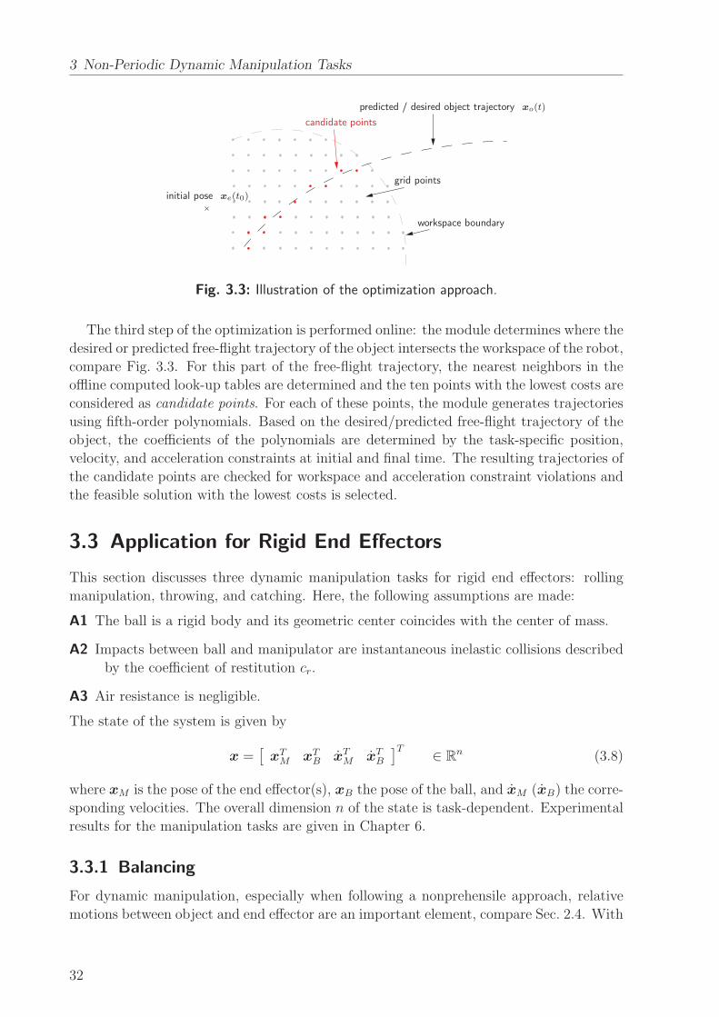
3 Non-Periodic Dynamic Manipulation Tasks
predicted / desired object trajectory
workspace boundary
candidate points
initial pose
grid points
xe(t0)
xo(t)
Fig. 3.3: Illustration of the optimization approach.
The third step of the optimization is performed online: the module determines where the
desired or predicted free-flight trajectory of the object intersects the workspace of the robot,
compare Fig. 3.3. For this part of the free-flight trajectory, the nearest neighbors in the
offline computed look-up tables are determined and the ten points with the lowest costs are
considered as candidate points. For each of these points, the module generates trajectories
using fifth-order polynomials. Based on the desired/predicted free-flight trajectory of the
object, the coefficients of the polynomials are determined by the task-specific position,
velocity, and acceleration constraints at initial and final time. The resulting trajectories of
the candidate points are checked for workspace and acceleration constraint violations and
the feasible solution with the lowest costs is selected.
3.3 Application for Rigid End Effectors
This section discusses three dynamic manipulation tasks for rigid end effectors: rolling
manipulation, throwing, and catching. Here, the following assumptions are made:
A1 The ball is a rigid body and its geometric center coincides with the center of mass.
A2 Impacts between ball and manipulator are instantaneous inelastic collisions described
by the coefficient of restitution cr.
A3 Air resistance is negligible.
The state of the system is given by
x =[
xTM xTB xTM xTB]T
∈ Rn (3.8)
where xM is the pose of the end effector(s), xB the pose of the ball, and xM (xB) the corre-
sponding velocities. The overall dimension n of the state is task-dependent. Experimental
results for the manipulation tasks are given in Chapter 6.
3.3.1 Balancing
For dynamic manipulation, especially when following a nonprehensile approach, relative
motions between object and end effector are an important element, compare Sec. 2.4. With
32
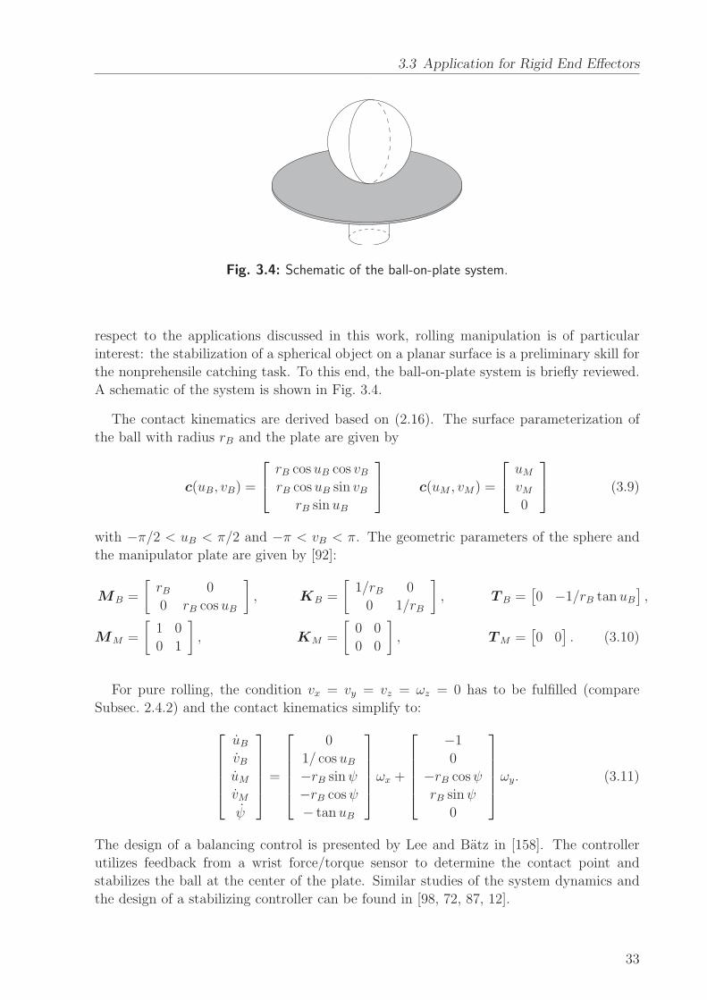
3.3 Application for Rigid End Effectors
Fig. 3.4: Schematic of the ball-on-plate system.
respect to the applications discussed in this work, rolling manipulation is of particular
interest: the stabilization of a spherical object on a planar surface is a preliminary skill for
the nonprehensile catching task. To this end, the ball-on-plate system is briefly reviewed.
A schematic of the system is shown in Fig. 3.4.
The contact kinematics are derived based on (2.16). The surface parameterization of
the ball with radius rB and the plate are given by
c(uB, vB) =
rB cos uB cos vBrB cos uB sin vB
rB sin uB
c(uM , vM) =
uMvM0
(3.9)
with −π/2 < uB < π/2 and −π < vB < π. The geometric parameters of the sphere and
the manipulator plate are given by [92]:
MB =
[
rB 0
0 rB cos uB
]
, KB =
[
1/rB 0
0 1/rB
]
, TB =[
0 −1/rB tan uB]
,
MM =
[
1 0
0 1
]
, KM =
[
0 0
0 0
]
, TM =[
0 0]
. (3.10)
For pure rolling, the condition vx = vy = vz = ωz = 0 has to be fulfilled (compare
Subsec. 2.4.2) and the contact kinematics simplify to:
uBvBuMvMψ
=
0
1/ cos uB−rB sinψ
−rB cosψ
− tan uB
ωx +
−1
0
−rB cosψ
rB sinψ
0
ωy. (3.11)
The design of a balancing control is presented by Lee and Batz in [158]. The controller
utilizes feedback from a wrist force/torque sensor to determine the contact point and
stabilizes the ball at the center of the plate. Similar studies of the system dynamics and
the design of a stabilizing controller can be found in [98, 72, 87, 12].
33
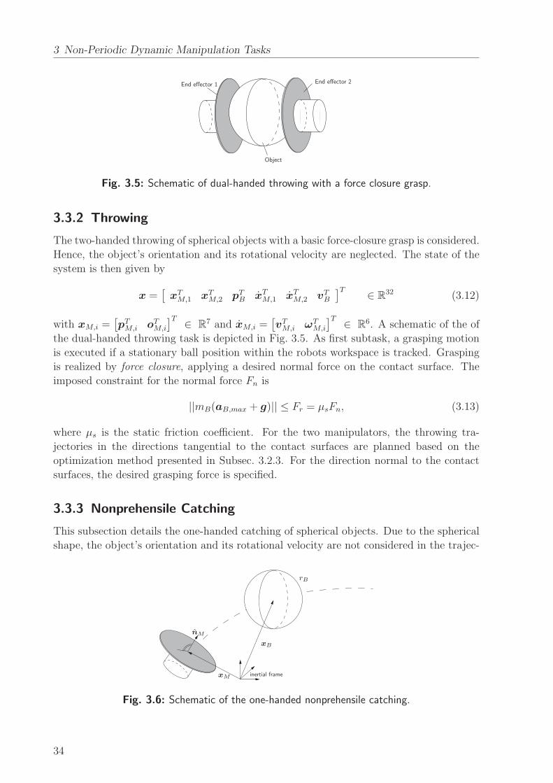
3 Non-Periodic Dynamic Manipulation Tasks
End effector 1 End effector 2
Object
Fig. 3.5: Schematic of dual-handed throwing with a force closure grasp.
3.3.2 Throwing
The two-handed throwing of spherical objects with a basic force-closure grasp is considered.
Hence, the object’s orientation and its rotational velocity are neglected. The state of the
system is then given by
x =[
xTM,1 xTM,2 pTB xTM,1 xTM,2 vTB]T
∈ R32 (3.12)
with xM,i =[
pTM,i oTM,i
]T∈ R
7 and xM,i =[
vTM,i ωTM,i
]T∈ R
6. A schematic of the of
the dual-handed throwing task is depicted in Fig. 3.5. As first subtask, a grasping motion
is executed if a stationary ball position within the robots workspace is tracked. Grasping
is realized by force closure, applying a desired normal force on the contact surface. The
imposed constraint for the normal force Fn is
||mB(aB,max + g)|| ≤ Fr = µsFn, (3.13)
where µs is the static friction coefficient. For the two manipulators, the throwing tra-
jectories in the directions tangential to the contact surfaces are planned based on the
optimization method presented in Subsec. 3.2.3. For the direction normal to the contact
surfaces, the desired grasping force is specified.
3.3.3 Nonprehensile Catching
This subsection details the one-handed catching of spherical objects. Due to the spherical
shape, the object’s orientation and its rotational velocity are not considered in the trajec-
inertial framexM
nM
xB
rB
Fig. 3.6: Schematic of the one-handed nonprehensile catching.
34
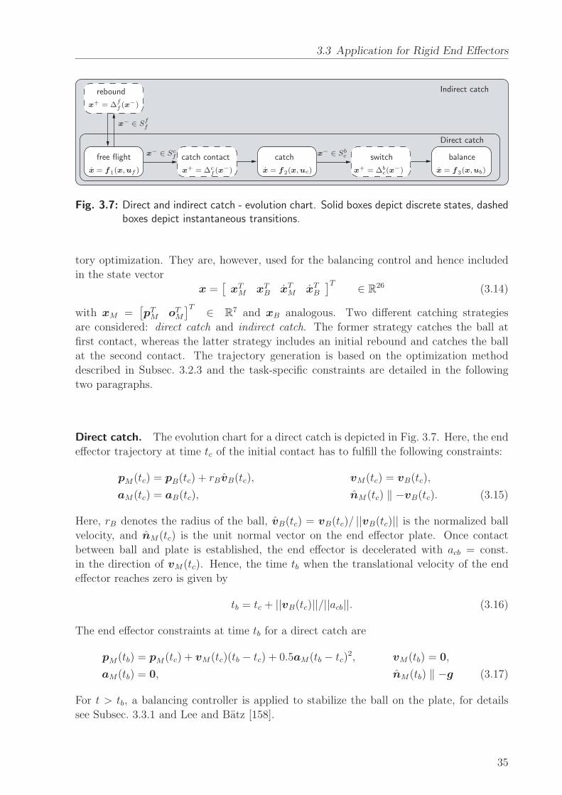
3.3 Application for Rigid End Effectors
free flight catch contact
rebound
catch balanceswitch
Indirect catch
Direct catch
x = f1(x,uf )
x− ∈ Scf
x+ = ∆cf(x−) x = f2(x,uc)
x− ∈ Sbc
x+ = ∆bc(x
−) x = f3(x,ub)
x− ∈ Sff
x+ = ∆ff(x−)
Fig. 3.7: Direct and indirect catch - evolution chart. Solid boxes depict discrete states, dashedboxes depict instantaneous transitions.
tory optimization. They are, however, used for the balancing control and hence included
in the state vector
x =[
xTM xTB xTM xTB]T
∈ R26 (3.14)
with xM =[
pTM oTM]T
∈ R7 and xB analogous. Two different catching strategies
are considered: direct catch and indirect catch. The former strategy catches the ball at
first contact, whereas the latter strategy includes an initial rebound and catches the ball
at the second contact. The trajectory generation is based on the optimization method
described in Subsec. 3.2.3 and the task-specific constraints are detailed in the following
two paragraphs.
Direct catch. The evolution chart for a direct catch is depicted in Fig. 3.7. Here, the end
effector trajectory at time tc of the initial contact has to fulfill the following constraints:
pM(tc) = pB(tc) + rBvB(tc), vM(tc) = vB(tc),
aM(tc) = aB(tc), nM(tc) ‖ −vB(tc). (3.15)
Here, rB denotes the radius of the ball, vB(tc) = vB(tc)/ ||vB(tc)|| is the normalized ball
velocity, and nM(tc) is the unit normal vector on the end effector plate. Once contact
between ball and plate is established, the end effector is decelerated with acb = const.
in the direction of vM(tc). Hence, the time tb when the translational velocity of the end
effector reaches zero is given by
tb = tc + ||vB(tc)||/||acb||. (3.16)
The end effector constraints at time tb for a direct catch are
pM(tb) = pM(tc) + vM(tc)(tb − tc) + 0.5aM(tb − tc)2, vM(tb) = 0,
aM(tb) = 0, nM(tb) ‖ −g (3.17)
For t > tb, a balancing controller is applied to stabilize the ball on the plate, for details
see Subsec. 3.3.1 and Lee and Batz [158].
35

3 Non-Periodic Dynamic Manipulation Tasks
Switching surface Reset map
Sff = ||vM ||+ λ ||pM − pB + rBnM || x+ = ∆f
f (x−) =
=[
xTM xTB xTM 01×2 cr ||vB|| ωTB
]T
Scf = ||vM − vB||+ λ ||pM − pB − rBvB|| x+ = ∆cf (x
−) = x−
Sbc = ||vM ||+ (xd − 2) x+ = ∆bc(x
−) = x−
Tab. 3.1: Indirect catch - switching surfaces and reset maps.
Indirect catch. If the direct catch algorithm does not obtain a feasible solution, the mod-
ule checks whether an indirect catch is possible in order to extend the range of admissible
object states. For an indirect catch, the following constraints are set for the end effector
trajectory at the initial contact time tr:
pM(tr) = pB(tr)− rBnM(tr), vM(tr) = 0, aM(tr) = 0, nM(tr) = −s/ ||s|| , (3.18)
where s = vB(tr) + g. With the assumptions A1 and A2, the last constraint ensures that
the ball rebounds in vertical z-direction. For the indirect catch, there is an additional phase
where the ball is again in free-flight, compare Fig. 3.7. The time tc of the second contact
at pM(tc) = pM(tr) is calculated based on the ball velocity vB(tr) and the coefficient of
restitution cr. The constraints at tc are then identical to the ones of a direct catch with
sole vertical velocity. The switching surfaces and reset maps for the indirect catch are
summarized in Tab. 3.1.
3.4 Summary
This chapter discussed non-periodic dynamic manipulation tasks using a generic end ef-
fector design. First, an overview of related work was given. Then, the planning of optimal
trajectories was discussed. The approach used in this work is based on a combination of
online and offline decisions: selection criteria are evaluated offline and look-up tables are
created. These look-up tables allow to evaluate the selection criteria online and to gener-
ate the desired trajectory. Section 3.3 presented three applications for rigid end effector
designs: Subsection 3.3.1 reviewed the ball-on-plate system since the stabilization of a
spherical object on a planar surface is a preliminary skill for nonprehensile manipulation.
Subsection 3.3.2 addressed the planning of dual-handed throwing motions. Here, the grasp-
ing of the object is realized with a basic force closure. Finally, Subsection 3.3.3 presented
a novel method for robotic catching: a nonprehensile approach was discussed which allows
the catching of bulky objects and the trajectory planning for catching spherical objects
was outlined. Two catching strategies, direct and indirect, were proposed to increase the
range of admissible initial object states. Both approaches considered the nonprehensile
catching of spherical objects. Here, the object orientation does not affect the geometry
of the contact surfaces. For arbitrarily shaped objects, the object orientation along the
trajectory has to be included as additional selection criteria. An experimental evaluation
of the studied manipulation tasks is presented in Chapter 6.
36
4 Periodic Manipulation Tasks with
Intermittent Contact
Summary This chapter considers periodic manipulation tasks with an intermittent con-
tact between actuator and object. Ball dribbling is introduced as a novel case study for
dynamic object manipulation. The system dynamics and optimal trajectory planning are
discussed for both a rigid and a compliant end effector design. The virtual holonomic
constraints approach is used to design a stabilizing controller for the dribbling task. In
addition, the classic juggling task is considered: the chapter reviews control strategies pro-
posed in the literature and presents a new approach for optimal trajectory planning based
on a non-local stability analysis.
The control of rhythmic tasks has been a very active research area over the last two
decades. A large amount of these research activities focused on legged robot locomotion.
However, besides robotic walking, there are also numerous works that investigated rhyth-
mic manipulation tasks which are commonly summarized with the term juggling. Buhler
coined the term for tasks that require interaction with an object or multiple objects that
would otherwise fall freely in the earths gravitational field [21]. For such tasks, the con-
tinuous motion of an actuator is used to control the continuous motion of one or multiple
objects through a temporary contact. Due to this intermittent or impulsive contact, the
systems possess hybrid dynamics described by discrete states with continuous dynamics
and instantaneous transitions.
The interest in juggling tasks originates from different sources: the first is the fact
that they provide an excellent scenario to investigate the role of feedback in rhythmic
tasks. Since the object is only controlled during a fraction of the cycle, the question
arises, in which phases sensor feedback is needed to stabilize a desired periodic motion. A
second, closely related aspect is the question of controllability of these systems. Due to the
underactuation of the system and the impulsive or intermittent character of the contact
phases, the control of these tasks is challenging. In addition, studying these manipulation
tasks can provide clues for the mechanical design of the manipulator. Finally, such periodic
tasks are helpful to increase the understanding of human movement control. The task of
juggling a ball, for instance, poses all the fundamental questions that are raised in the
study of human motion coordination, see [117]. Finally, due to their periodicity, these
tasks are well suited for the evaluation of learning algorithms.
The chapter is organized as follows: Section 4.1 provides an overview on related work.
37

4 Periodic Manipulation Tasks with Intermittent Contact
In Section 4.2, the planning of optimal trajectories for periodic manipulation tasks is ad-
dressed. Section 4.3 discusses the stability of periodic solutions of ordinary differential
equations. Next, Section 4.4 addresses the stability of periodic solutions of hybrid dynam-
ical systems. In addition to local stability, the section also considers a region of attraction
analysis. Section 4.5 then applies these methods to tasks with a rigid manipulator. Besides
the classic juggling, the task of dribbling a ball is considered as it introduces additional
challenges. The distinctive feature of the dribbling task is the existence of a second, au-
tonomous impact between the object and the environment. Finally, Section 4.6 details the
realization of the dribbling task with a compliant end effector.
4.1 Related Work
Holmes was the first to investigate the dynamics of repeated impacts on a sinusoidally
vibrating table [54]. With this work, he introduced the bouncing ball model as a case
study in nonlinear dynamics which has since become very popular. Holmes proved that, for
sufficiently large excitation velocities and a coefficient of restitution close to one, the system
possesses both periodic solutions as well as irregular non-periodic and chaotic motions.
Inspired by Holmes pioneering work, various researchers have considered this or similar
tasks: Bapat and coworkers followed up the work of Holmes, focusing on the sinusoidal
motions which led to stable periodic collisions [5]. Their results already implied that such a
sinusoidal actuation requires negative actuator acceleration at impact to obtain open-loop
stability. Based on a refinement of Holmes original model, the numerical simulations of
Luo and Han led to an extended range of stable periodic motions [80].
Buhler et al. were the first to investigate the stabilization of robotic juggling
tasks [20, 21, 22]. In their work, they considered the trajectory control of a puck which
was constrained to lie on a plane turned into the earth’s gravitational field. The manip-
ulator was a one DOF robot with a revolute joint. They proposed the so called mirror
law algorithm for stabilizing the desired periodic motions of the puck. Here, the idea is
that the manipulator describes a distorted reflection (mirroring) of the objects trajectory.
The control algorithm was verified for a planar experimental setup. However, it should
be noted that the mirror law does not provide open-loop stability and hence requires per-
manent tracking of the ball. Following the work of Buhler, Rizzi et al. extended the
mirror law to accomplish spatial juggling of two balls with a three DOF robot manipula-
tor [104, 105, 107, 23].
Atkeson and Schaal investigated the learning of different periodic manipulation tasks,
e.g. devil sticking and classic juggling. Here, they demonstrated that task-level learning
improves the performance of a juggling robot [2, 116, 115]. In addition, Schaal and Atkeson
discussed open-loop stability for the classic juggling task. Generalizing the results of
Holmes and Bapat, they showed that, for a line juggler, an arbitrary periodic motion of
the manipulator results in open loop stability if the manipulator acceleration at impact is
within a certain negative range [114]. Considering systems with one DOF object motion,
this is an fundamental advantage compared to the mirror algorithm as this approach allows
sensorless stabilization of a desired periodic orbit. For planar or spatial juggling systems,
however, it is important to note that the open-loop control can not stabilize a particular
38

4.2 Trajectory Planning
contact point in the impact plane. Horizontal deviations still have to be compensated by an
additional control or an appropriate mechanical design, see e.g. [102]. Schaal and Atkeson
also provided a non-local stability analysis for the open loop stable control strategies [117].
However, this analysis is of limited use since it does not determine a region of attraction
but only allows relative comparisons of different controller designs. Based on these results,
Schaal and Sternard also published a number of studies that focused on human motion
coordination in a classic juggling task [117, 133, 134].
Driven by the interest in minimalist manipulation systems, Lynch and Black discussed
the planar juggling system with one actuated revolute joint introduced by Buhler. Here,
the planar juggler served as a case study for systems that are controllable, but insufficient
actuated to be locally controllable. Applying the idea of forced recurrence, they showed
controllability of the system on a large subspace of the state space and developed a stabi-
lizing controller [81]. Brogliato et al. also discussed controllability and proposed stabilizing
feedback laws for the one DOF and the planar juggler [19, 150].
A special type of juggling system, the so called wedge billiard, was first introduced by
Lehtitet and Miller and later studied in detail by Sepulchre et al. [121, 77]. Such dynam-
ical billiards are part of the mathematical theory of particle trajectories within a closed
reflective boundary. Ronsse and Sepulchre studied different types of actuation and inves-
tigated the importance of timing the control feedback [108, 109, 110]. They also discussed
feedback control strategies for the bouncing ball system and discussed the influence of the
impact acceleration on the robustness of the system to parameter uncertainties [112].
An example of robot dribbling was presented by Shiokata et al. for experimental eval-
uation of a high-speed vision system [122]. For the experiment, a ping-pong ball and
an actuator with four DOF were used. The task served as a benchmark study for the
high-speed vision system and did not discuss the trajectory planning or the design of a
stabilizing controller.
Besides their periodic nature, the works discussed so far all have the characteristic
property of an intermittent and/or impulsive contact in common. For the sake of com-
pleteness, it has to be mentioned that there exist also numerous periodic/rhythmic dynamic
manipulation tasks with continuous contact phases. An interesting example is the work
of Zacksenhouse et al. who investigated robotic yo-yo playing [62, 63, 61]. However, these
works are not further discussed as the focus of the chapter is on periodic manipulation
tasks with intermittent contact.
4.2 Trajectory Planning
The trajectory planning for periodic tasks is similar to the one for non-periodic which was
presented in Sec. 3.2. Again, the planning is based on the modeling foundations discussed in
Ch. 2. As detailed in Sec. 3.2, equality constraints ce(γ) = 0 are used to specify positions,
velocities, and accelerations at certain points in time and inequality constraints ci(γ) ≤ 0
are used to incorporate hardware limitations. The same approach and the same selection
criteria as for the tasks studied in Sec. 3 can be applied for the trajectory optimization
of periodic manipulation tasks, compare (3.4)-(3.7). The trajectory planning for periodic
manipulation tasks also includes on- and offline decisions. However, the periodic nature of
39

4 Periodic Manipulation Tasks with Intermittent Contact
the tasks allows more offline decisions in the planning process.
Considering the open-loop control of a periodic manipulation task, the manipulator
motion is described by an arbitrary but periodic trajectory. Hence, the motion of the
manipulator can be described by a finite Fourier series
xM(t) =L∑
k=1
Ak sin (kωt+ φk) . (4.1)
Consequently, position, velocity, and acceleration of the manipulator at time tn (at the
n-th impact) are given by
xM [n] =L∑
k=1
Ak sin (kωtn + φk) = f(ωtn) = f(θ[n]),
xM [n] = ω
L∑
k=1
Akk cos (kωtn + φk) = ωf ′(ωtn) = ωf ′(θ[n]), (4.2)
xM [n] = ω2
L∑
k=1
−Akk2 sin (kωtn + φk) = ω2f ′′(ωtn) = ω2f ′′(θ[n]),
where the expressions f ′(θ[n]) =∂f(θ[n])
∂θ[n]and f ′′(θ[n]) =
∂2f(θ[n])
∂2θ[n]have been used [134].
4.3 Stability of Periodic Solutions of Ordinary Differential
Equations
This section outlines definitions that are preliminary for the stability analysis of hybrid
systems in Sec. 4.4. A detailed discussion of these definitions can be found in the books
by Parker and Chuo, Khalil, and Slotine [99, 69, 129]. In the following, an autonomous
continuous-time dynamical system x = f(x) as defined in (2.2) is considered. By assuming
a state feedback control u = k(x), the explicit dependency of the system on the control
input u is omitted.
Definition 4.1 (Periodic solution, Periodic orbit, Limit cycle) The flow φt(x0) is
a periodic solution (orbit) Γ of an autonomous system if, for all t,
φt(x0) = φt+T (x0) (4.3)
for some period T > 0. The restriction T > 0 is needed to prevent the classification of
an equilibrium point as periodic solution. A periodic solution is isolated if it possesses a
neighborhood that contains no other periodic solution. In the autonomous case, an isolated
periodic solution is called a limit cycle. The limit set corresponding to a limit cycle is the
closed curve defined by φt(x0) over one period.
Typically, in a nonlinear dynamical system, there exist other limit sets in addition to the
periodic solution such as equilibrium points, quasi-periodic solutions and chaos. The focus
40

4.3 Stability of Periodic Solutions of Ordinary Differential Equations
in this chapter, however, is the study of periodic solutions.
Definition 4.2 (Invariant set) A set M is said to be an invariant set with respect to
an autonomous ODE (2.2) if
x(t0) ∈M ⇒ x(t) ∈M, ∀ t ≥ R (4.4)
Hence, a periodic solution φt(x0) is a closed invariant set of the dynamic system (2.2). In
the following, the periodic solution is denoted by Γ.
Definition 4.3 (LaSalle’s invariance principle) Consider an autonomous ODE as de-
fined in (2.2) and let V (x) : Rn → R be a locally positive definite function. Assume that,
on the compact set
Ωl = x ∈ Rn : V (x) ≤ l , it holds that V (x) ≤ 0 ∀ x ∈ Ωl.
Define R = x ∈ Ωl : V (x) = 0 and let M be the largest invariant set in R. Then, every
solution x(t) originating in Ωl tends to M as t→ ∞.
Definition 4.4 (Discrete-time dynamical system) A discrete dynamical system is
defined by
x[k+1] = f d(x[k]) k = 0, 1, 2, . . . (4.5)
where x[k] ∈ Rn is the state and f d : D ⊂ R
n → Rn maps the current state x[k] to the
next state x[k+1].
Poincare map. The Poincare map is a widely used technique for the analysis of dynamical
systems. Here, the flow of an n-th order dynamical system is replaced with an (n− 1)-th
order discrete-time system which is called the Poincare map. Its main advantages are the
reduction of order and the fact that it bridges the gap between continuous- and discrete-
time systems [99].
Definition 4.5 (Poincare map, First return map for autonomous systems)
Consider an n-th order autonomous system with the limit cycle (periodic orbit) Γ
as shown in Fig. 4.1. Let x∗ denote a point on the limit cycle and let Σ be an
(n − 1)-dimensional cross section (hyperplane) transversal to Γ at x∗. A cross section is
transversal, if n(x)Tf(x) 6= 0, where n is the normal vector to Σ. Then, the Poincare
map P : U → Σ is defined in a neighborhood U ⊂ Σ of x∗ as
P (x) := φT (x)(x). (4.6)
The time T (x) denotes the first time the orbit and the cross section intersect after starting
the integration in x ⊂ U . The mapping has a fixed point if P (x∗) = x∗.
Due to the definition of the Poincare map, its limit sets correspond to the limit sets of
the underlying flow. Furthermore, the asymptotic stability of the fixed point can be shown
to be equivalent to the asymptotic orbital stability of the periodic solution. A fixed point
41

4 Periodic Manipulation Tasks with Intermittent Contact
x
P (x)
x∗ = P (x∗)
Σ
Γ
Fig. 4.1: Poincare map
x∗ of the nonlinear difference equation x[n+1] = P (x[n]) can be shown to be asymptotically
stable if all eigenvalues of its linearization
∂P (x)
∂x
∣
∣
∣
∣
x=x∗
(4.7)
are strictly within the unit circle [99, 130].
Topological equivalence of flows. The concept of equivalence is a useful tool for the
comparison of (hybrid) dynamical systems. Two orbits of a smooth or hybrid dynamical
system are topologically orbitally equivalent (TOE) if there exists a orientation-preserving
homeomorphism that maps one orbit into the other [60, 128]. Employing the TOE helps to
simplify the analysis of periodic solutions: if such a homeomorphism exists, the results of a
particular periodic solution can be generalized to other periodic orbits, see e.g. Schaal [134].
4.4 Stability of Periodic Solutions of Hybrid Dynamical
Systems
The following section outlines methods for local and global stability analysis of hybrid
systems. A hybrid system as stated in Definition 2.3 is considered. However, the explicit
dependence on the control inputs u and ud is omitted by assuming a state-dependent
control law in the form u = k(x, xd) and ud = k(x, xd). The hybrid system is then given
by
x = f i(x, xd) if sji (x, xd) /∈ 0 ∀ i, j,
ζ+ =
[
x+
x+d
]
=
[
∆ji (x
−, xd)
j
]
if sji (x, xd) = 0. (4.8)
4.4.1 Local Stability Analysis
The concepts for local stability analysis of periodic solutions of hybrid system are analogous
to the ones for ODEs discussed in Sec. 4.3.
42
4.4 Stability of Periodic Solutions of Hybrid Dynamical Systems
Definition 4.6 (Hybrid periodic solution, Hybrid periodic orbit) A solution of ζ
is a hybrid periodic solution Γ with period length T > 0 if
ζ(t+ T ) = ζ(t), (4.9)
holds for all t ∈ R.
This definition of a hybrid periodic solution implies that there exists a switching sequence
of the discrete state xd which corresponds to the periodic solution.
A general definition for the stability of invariant sets of hybrid dynamical systems was
given by Simic et al. [127]. In most works that consider the stability of hybrid periodic
solutions, the stability of the hybrid limit cycle is determined with the stability of the
discrete mapping of the hybrid Poincare map [130, 51].
Poincare map for hybrid systems. The definition of the hybrid Poincare map is in
accordance with the one for smooth dynamical systems stated in Def. (4.5). Assume a
cross section Σ that is transversal to the flow of the hybrid system. Then, the hybrid
Poincare map is defined to map initial values on Σ to the next occurrence of a crossing of
Σ. A detailed discussion on the construction of the hybrid Poincare map is provided by
Sobotka in [130].
4.4.2 Non-Local Stability Analysis
The Poincare map is a powerful tool and a widely used technique for the local stability
analysis of periodic solutions for hybrid dynamical systems. However, the eigenvalues of
the linearized system dynamics provide only a local stability measure. In order to evaluate
the robustness of a hybrid periodic orbit with respect to disturbances or to modeling
errors, it is important to know how the system behaves in the non-local neighborhood of
the periodic solution.
Region of attraction. The behavior in the neighborhood of the hybrid limit cycle can be
evaluated with a region of attraction analysis. Such an analysis addresses the shortcomings
of the Poincare map and determines a region in which initial states are attracted to the
periodic orbit. Following a numerical approach, the region of attraction is estimated by
simulating the system’s hybrid flow for initial states in the vicinity of the desired fixed
point. For a dense grid of sample points, the convergence/divergence of the corresponding
flows determines an attracting region for the hybrid limit cycle. A cell mapping method
can be used to reduce the computational burden of the numerical approach [56]. Schwab
and Wisse employed this method to evaluate the attracting region of a periodic orbit for
a passive walking model [118]. The approach can be used for systems with either open- or
closed-loop control.
43
4 Periodic Manipulation Tasks with Intermittent Contact
4.5 Application for Rigid End Effectors
In this section, a rigid manipulator design is assumed and two periodic manipulation tasks
with intermittent contact are considered: classic juggling and dribbling. For both tasks,
the dynamic model and the first return map are derived. Based on the model, a local
and global stability is performed. For the model and the stability analysis, the following
assumptions are made:
A1 The ball and the manipulator are modeled as one DOF systems such that only vertical
motions are taken into account.
A2 The ball is a rigid body and its geometric center coincides with the center of mass.
A3 Impacts between ball and manipulator and (possible) impacts between ball and ground
are instantaneous inelastic collisions described by the coefficient of restitution cr.
A4 Air resistance and rotational ball velocity are negligible.
4.5.1 Classic Juggling Task
A schematic of the juggling system is depicted in Fig. 4.2. The manipulator is used to
control the motion of the object through an instantaneous contact.
Review of control strategies. Different solutions have been reported in literature to
realize stable periodic motions for the juggling task. A sinusoidal trajectory
xM(t) = A sin(ωt+ φ0) + xM,0 (4.10)
which does not require any sensory feedback has been first proposed by Holmes and later
by Schaal et al. [54, 114]. Next, Buhler et al. presented a mirror law
xM(t) =
(
−1− cr1 + cr
− κ (E∗ − E(t))
)
xB(t), (4.11)
that requires permanent tracking of the ball [21, 22, 104, 105, 107]. Here, E∗ and E(t)
denote the desired and the actual ball energy. Finally, a trajectory based on state-feedback
xM(t) = xM [n+1] + xM [n+1]
(
t− t[n+1]
)
+1
2xM [n+1]
(
t− t[n+1]
)2(4.12)
for t[n] < t < t[n+1] has been discussed by Ronsse et al. [110, 111]. For the three strategies,
the manipulator position xM and velocity xM at impact are determined by the desired
periodic motion. The manipulator acceleration xM , in contrast, is a free parameter.In the
following, the optimal open-loop control strategy for the juggling task is evaluated.
Dynamic model. The state of the system is described by the position and velocity of the
manipulator and the ball,
x =[
xM xB xM xB]T. (4.13)
44
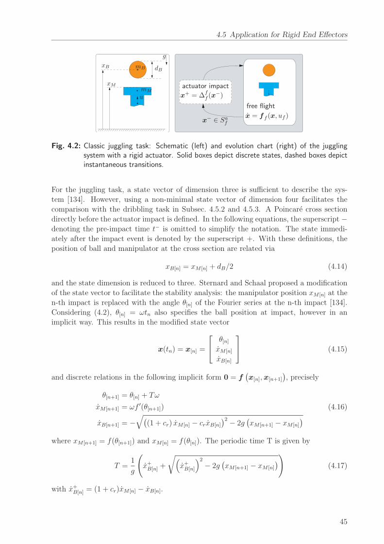
4.5 Application for Rigid End Effectors
mM
mBxB
xM
g
u
dB
free flight
actuator impact
x = ff (x, uf )
x+ = ∆ff (x
−)
x− ∈ Saf
Fig. 4.2: Classic juggling task: Schematic (left) and evolution chart (right) of the jugglingsystem with a rigid actuator. Solid boxes depict discrete states, dashed boxes depictinstantaneous transitions.
For the juggling task, a state vector of dimension three is sufficient to describe the sys-
tem [134]. However, using a non-minimal state vector of dimension four facilitates the
comparison with the dribbling task in Subsec. 4.5.2 and 4.5.3. A Poincare cross section
directly before the actuator impact is defined. In the following equations, the superscript −
denoting the pre-impact time t− is omitted to simplify the notation. The state immedi-
ately after the impact event is denoted by the superscript +. With these definitions, the
position of ball and manipulator at the cross section are related via
xB[n] = xM [n] + dB/2 (4.14)
and the state dimension is reduced to three. Sternard and Schaal proposed a modification
of the state vector to facilitate the stability analysis: the manipulator position xM [n] at the
n-th impact is replaced with the angle θ[n] of the Fourier series at the n-th impact [134].
Considering (4.2), θ[n] = ωtn also specifies the ball position at impact, however in an
implicit way. This results in the modified state vector
x(tn) = x[n] =
θ[n]xM [n]
xB[n]
(4.15)
and discrete relations in the following implicit form 0 = f(
x[n],x[n+1]
)
, precisely
θ[n+1] = θ[n] + Tω
xM [n+1] = ωf ′(θ[n+1]) (4.16)
xB[n+1] = −
√
(
(1 + cr) xM [n] − crxB[n]
)2− 2g
(
xM [n+1] − xM [n]
)
where xM [n+1] = f(θ[n+1]) and xM [n] = f(θ[n]). The periodic time T is given by
T =1
g
(
x+B[n] +
√
(
x+B[n]
)2
− 2g(
xM [n+1] − xM [n]
)
)
(4.17)
with x+B[n] = (1 + cr)xM [n] − xB[n].
45

4 Periodic Manipulation Tasks with Intermittent Contact
Local stability analysis. For the local stability analysis, the system (4.16) is linearized
around the fixed point using the implicit function theorem [134]. The linearization is given
by
∂P (x)
∂x
∣
∣
∣
∣
x=x∗
=
1 −ωcr(1 + cr)/g (1 + cr)2ω/g
0 c2r −cr(1 + cr)
ωf ′′(θ[n]) −ω2f ′′(θ[n])cr(1 + cr)/g ω2f ′′(θ[n])(1 + cr)2/g
. (4.18)
The system (4.16) has an asymptotically stable fixed point x∗ if all eigenvalues of the
linearization (4.18) are strictly within the unit circle, compare Def. 4.5 and [99]. This is
the case if the condition−2(1 + c2r)g
(1 + cr)2< xM [n] < 0 (4.19)
is fulfilled [116]. Depending on cr, the lower bound varies between −g (cr = 1) and −2g
(cr = 0).
Non-local stability analysis. A non-local stability analysis for the classic juggling task
was presented by Schaal et al. [117]. The analysis was based on a discrete-time Lyapunov
function Ln for the linearized system. The state was sampled around the equilibrium state
x∗ and, for each of sample i, the relative change ∆Li = Li,[n+1] − Li,[n] was determined.
By summarizing over all samples, a stability measure S =∑
i∆Li is obtained. This
approach has several drawbacks: first, the range of validity of the analysis is limited since
the Lyapunov function is based on the linearized system. Second, the overall stability
measure does not provide information about which initial states converge to the periodic
orbit. Finally, the relative change ∆Li over one period is of limited use since a convergence
towards the orbit could occur over multiple cycles. Due to these limitations, the method
presented in Subsec. 4.4.2 is better suited to estimate the region of attraction.
Fixed points that possess a large region of attraction are desirable since larger distur-
bances and modeling errors can be compensated. The following two paragraphs describe
the chosen numerical approach to analyze the region of attraction for the juggling task.
Manipulator acceleration. For this analysis, the coefficient of restitution was assumed
to be cr = 0.7 and the periodic time T was set to 0.4 s. These assumptions define the
desired fixed point as
x∗ =[
x∗M x∗B x∗M x∗B]T
=[
0 0 0.3462 −1.962]T. (4.20)
The relation derived in (4.19) states a regime of manipulator accelerations x∗M that result
in local stability of the fixed point. In order to investigate the interdependence between
the manipulator acceleration and the size of the region of attraction, the manipulator
trajectory is optimized for a number of fixed x∗M . To this end, the system is initialized
at equidistant grid points xj in the vicinity of the fixed point x∗ and then simulated for
Nc = 20 cycles. In the vicinity of the desired impact, the periodic manipulator trajectory
46
4.5 Application for Rigid End Effectors
(4.2) can be approximated by a sixth-order polynomial [117]
xM(t) =6∑
k=0
ak(t− tn)k for ||t− tn|| ≤ tthresh. (4.21)
For a sampling point xj, the initial and final error are defined as
ei,j =
√
(
xj[1] − x∗)T (
xj[1] − x∗)
ef,j =
0, if√
(
xj,[Nc] − x∗)T (
xj,[Nc] − x∗)
≤ ethresh
ej,max else,(4.22)
where ej,max is the maximum error that occurred at the last five impacts. Using the
maximum error allows to identify chaotic behavior that might, by accident, show a relative
small error for the final cycle of the simulation. With (4.22), the relative change of the
error erel,j = ef,j/ei,j can be determined for each grid point xj. The trajectory optimization
utilizes a cost function that combines the relative change of the error for each sample point
xj. The optimization problem is given by
minγ∈Γ
J(γ) = λNs∑
j=1
(
ef,jei,j
)2
with Γ =
γ ∈ R7, ci(γ) ≤ 0, ce(γ) = 0
(4.23)
γ = [a0, . . . , a6]
Here, λ = 102 and the number of grid points is Ns = 357 (21 along ∆xB and 17 along ∆T ).
The inequality constraints ci(γ) restrict the manipulator trajectory to feasible motions.
The equality constraints ce(γ) are determined by the desired fixed point x∗ and the desired
manipulator acceleration,
ci(γ) =
||a3|| − 102
...
||a6|| − 102
ce(γ) =
a0 − x∗Ma1 − x∗Ma2 − x∗M
. (4.24)
The results of the optimization for six manipulator accelerations in the range from
xM = 0.0 m/s2 to xM = −7.5 m/s2 are illustrated in Fig. 4.3. The coefficient of restitution
was assumed to be cr = 0.7 and the periodic time T was set to 0.4 s. For the cases (b)
to (f), regions of attraction (white areas) around the fixed point x∗ are found. However,
no attracting region is found for case (a) with xM = 0 m/s2. This corresponds to the
result of (4.19) which determines zero manipulator acceleration at the impact as locally
unstable. While there is a relatively large region of attraction for xM = −1.5 m/s2, it
reduces with decreasing xM . This is also illustrated in Tab. 4.1, where the optimized costs
J for different manipulator accelerations xM are summarized. Based on these results, a
manipulator trajectory with an acceleration x∗M at impact in the range of [−0.5, −2] m/s2
is desirable as this maximizes the region of attraction.
47
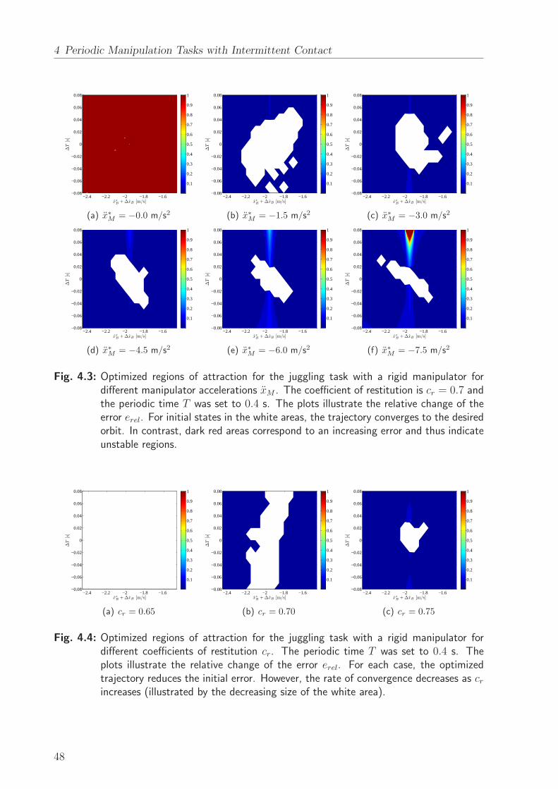
4 Periodic Manipulation Tasks with Intermittent Contact
−2.4 −2.2 −2 −1.8 −1.6−0.08
−0.06
−0.04
−0.02
0
0.02
0.04
0.06
0.08
x∗B + ∆xB [m/s]
∆T
[s]
0.1
0.2
0.3
0.4
0.5
0.6
0.7
0.8
0.9
1
(a) x∗
M = −0.0 m/s2
−2.4 −2.2 −2 −1.8 −1.6−0.08
−0.06
−0.04
−0.02
0
0.02
0.04
0.06
0.08
x∗B + ∆xB [m/s]∆
T[s]
0.1
0.2
0.3
0.4
0.5
0.6
0.7
0.8
0.9
1
(b) x∗
M = −1.5 m/s2
−2.4 −2.2 −2 −1.8 −1.6−0.08
−0.06
−0.04
−0.02
0
0.02
0.04
0.06
0.08
x∗B + ∆xB [m/s]
∆T
[s]
0.1
0.2
0.3
0.4
0.5
0.6
0.7
0.8
0.9
1
(c) x∗
M = −3.0 m/s2
−2.4 −2.2 −2 −1.8 −1.6−0.08
−0.06
−0.04
−0.02
0
0.02
0.04
0.06
0.08
x∗B + ∆xB [m/s]
∆T
[s]
0.1
0.2
0.3
0.4
0.5
0.6
0.7
0.8
0.9
1
(d) x∗
M = −4.5 m/s2
−2.4 −2.2 −2 −1.8 −1.6−0.08
−0.06
−0.04
−0.02
0
0.02
0.04
0.06
0.08
x∗B + ∆xB [m/s]
∆T
[s]
0.1
0.2
0.3
0.4
0.5
0.6
0.7
0.8
0.9
1
(e) x∗
M = −6.0 m/s2
−2.4 −2.2 −2 −1.8 −1.6−0.08
−0.06
−0.04
−0.02
0
0.02
0.04
0.06
0.08
x∗B + ∆xB [m/s]
∆T
[s]
0.1
0.2
0.3
0.4
0.5
0.6
0.7
0.8
0.9
1
(f) x∗
M = −7.5 m/s2
Fig. 4.3: Optimized regions of attraction for the juggling task with a rigid manipulator fordifferent manipulator accelerations xM . The coefficient of restitution is cr = 0.7 andthe periodic time T was set to 0.4 s. The plots illustrate the relative change of theerror erel. For initial states in the white areas, the trajectory converges to the desiredorbit. In contrast, dark red areas correspond to an increasing error and thus indicateunstable regions.
−2.4 −2.2 −2 −1.8 −1.6−0.08
−0.06
−0.04
−0.02
0
0.02
0.04
0.06
0.08
x∗B + ∆xB [m/s]
∆T
[s]
0.1
0.2
0.3
0.4
0.5
0.6
0.7
0.8
0.9
1
(a) cr = 0.65
−2.4 −2.2 −2 −1.8 −1.6−0.08
−0.06
−0.04
−0.02
0
0.02
0.04
0.06
0.08
x∗B + ∆xB [m/s]
∆T
[s]
0.1
0.2
0.3
0.4
0.5
0.6
0.7
0.8
0.9
1
(b) cr = 0.70
−2.4 −2.2 −2 −1.8 −1.6−0.08
−0.06
−0.04
−0.02
0
0.02
0.04
0.06
0.08
x∗B + ∆xB [m/s]
∆T
[s]
0.1
0.2
0.3
0.4
0.5
0.6
0.7
0.8
0.9
1
(c) cr = 0.75
Fig. 4.4: Optimized regions of attraction for the juggling task with a rigid manipulator fordifferent coefficients of restitution cr. The periodic time T was set to 0.4 s. Theplots illustrate the relative change of the error erel. For each case, the optimizedtrajectory reduces the initial error. However, the rate of convergence decreases as crincreases (illustrated by the decreasing size of the white area).
48

4.5 Application for Rigid End Effectors
Manipulator acceleration xM [m/s2]
0.0 −1.5 −3.0 −4.5 −6.0 −7.5 −9.0
Costs J 9.4 · 107 3.2 7.3 13.5 69.3 3.8 · 103 2.5 · 105
Tab. 4.1: Optimized costs J for different manipulator accelerations xM with cr = 0.7.
Coefficient of restitution cr0.60 0.625 0.65 0.675 0.70 0.725 0.75
Costs J 0 0 0 0.007 0.61 3.09 9.56
Tab. 4.2: Optimized costs J for different coefficients of restitution cr with optimized x∗M .
Coefficient of restitution. In contrast to the manipulator acceleration, the coefficient
of restitution cr is a task-specific parameter which is determined by the properties of the
colliding bodies, compare Sec. 2.6. Consequently, the value of cr can not be the subject
of an optimization process. However, (4.19) showed that cr influences the local stability.
Hence, it is interesting to see which effect cr has on the region of attraction. To this
end, a second numerical optimization was performed for different values of cr. In this
optimization, the manipulator acceleration xM is a free parameter. The results of the
optimization for three values of cr are depicted in Fig. 4.4(a)-(c). Again, the periodic
time T was set to 0.4 s. For each case, the optimized trajectory reduces the initial error.
However, as illustrated by the decreasing white areas, the rate of convergence slows down
for increasing values of cr. This is also shown in Tab. 4.2, which summarizes the optimized
costs J for cr in the range from 0.60 to 0.75.
4.5.2 Dribbling Task
The schematic setup and the evolution chart of the dribbling task with a rigid end effector
is illustrated in Fig. 4.5. The fundamental difference to the juggling task is the existence
of an additional, autonomous impact that occurs between ball and ground. Due to this
additional impact, a periodic solution for the dribbling task is defined by x∗M , x∗M , and
x∗B. For the juggling task, x∗M and x∗M sufficed to define a periodic solution, compare
Subsec.4.5.1.
Dynamic model. Again, a Poincare cross section directly before the actuated impact
is considered and the superscript − for the state is omitted. The position of ball and
manipulator at the cross section are then related via
xB[n] = xM [n] − dB/2 (4.25)
and the state dimension is reduced to three. The time of the ground impact is denoted
by tgi and x+B,gi[n] = xB[n]
(
t+gi)
refers to the ball velocity after the n-th ground impact.
With the state vector introduced in (4.15), the discrete-time dynamic model of the system
49

4 Periodic Manipulation Tasks with Intermittent Contact
actuator impact
free flight
ground impact
mM
mBxB
xM
gu
dB
x = ff (x, uf )
x+ = ∆ff (x
−) x+ = ∆ff (x
−)
x− ∈ Saf
x− ∈ Sgf
Fig. 4.5: Dribbling task: schematic (left) and evolution chart (right) of the dribbling systemwith a rigid actuator. Solid boxes depict discrete states, dashed boxes depict instan-taneous transitions.
is given by integration of the continuous-time dynamics
θ[n+1] = θ[n] + Tω
xM [n+1] = ωf ′(θ[n+1])
xB[n+1] = −gTrise + x+B,gi[n] = (4.26)
=
√
(
x+B,gi[n]
)2
− 2gf(θ[n+1]) =
√
c2r
(
−gTdrop + x+B[n]
)2
− 2gf(θ[n+1])
=
√
c2r(
(1 + cr)xM [n] − crxB[n]
)2+ 2gc2r
(
f(θ[n])− dB)
− 2gf(θ[n+1])
with the following abbreviations:
x+B[n] = (1 + cr)xM [n] − crxB[n], x+B,gi[n] = −crx−B,gi[n] = −cr(−gTdrop + x+B[n]),
Tdrop =1
g
(
x+B[n] +
√
(
x+B[n]
)2
+ 2g(
xM [n] − dB)
)
, (4.27)
Trise =1
g
(
x+B,gi[n] −
√
(
x+B,gi[n]
)2
− 2gxM [n+1]
)
.
Local stability analysis. For the local stability analysis, the system (4.26) is also lin-
earized around the fixed point using the implicit function theorem. The linearization of
the Poincare map ∂P (x)∂x
∣
∣
∣
x=x∗
can be derived analytically and results in a long symbolic
expression. For the dribbling task, the linearized matrix and its eigenvalues are a function
of the chosen fixed point x∗. This is in contrast to the juggling task, where the eigenvalues
were not influenced by the fixed point x∗, compare (4.18)-(4.19). Due to this increased
complexity, it is not possible to derive an analytical expression for the range of locally
stable periodic orbits for the dribbling task. However, it is possible to perform a numerical
analysis which evaluates the stability properties for different hybrid limit cycles. For the
dribbling task, a periodic solution is defined by x∗M , x∗M , and x∗B.
In the following analysis, the ball velocity before the actuated impact x∗B is constrained
50

4.5 Application for Rigid End Effectors
−30 −25 −20 −15 −10 −5 0 5 10
−2.5
−2.4
−2.3
−2.2
−2.1
−2
−1.9
manipulator acceleration xM [m/s2]
man
ipula
tor
vel
oci
tyx
M[m
/s]
(a) fixed manipulator position x∗
M = 1.4 m
−30 −25 −20 −15 −10 −5 0 5 100.8
1
1.2
1.4
1.6
1.8
2
manipulator acceleration xM [m/s2]
man
ipula
tor
pos
itio
nx
M=
f(θ
)[m
]
(b) fixed manipulator velocity x∗
M = −2.2 m/s
Fig. 4.6: Local stability of periodic solutions of the dribbling task for cr = 0.8. Green circlesdenote locally stable combinations where the magnitude of the largest eigenvalue issmaller than one. A large marker corresponds to a small maximum eigenvalue. Redcrosses denote unstable solutions and black squares illustrate infeasible solutions.
to the range [0, 5] m/s. If there exist two feasible ball velocities within the range for a
given combination of x∗M and x∗B, the velocity with the smaller absolute value is chosen.
The coefficient of restitution is assumed to be cr = 0.8. With these assumptions, a local
stability analysis for different periodic solutions can be performed by varying the manipu-
lator position x∗M and velocity x∗M at impact. Fig. 4.6 illustrates the relationships between
these two quantities, the manipulator acceleration xM and the magnitude of the largest
eigenvalue for the linearized system. Fig.4.6(a) shows combinations of manipulator accel-
erations and velocities for a fixed position x∗M = 1.4 m. Fig.4.6(b) shows combinations of
manipulator accelerations and positions for a fixed manipulator velocity x∗M = −2.2 m/s.
In both cases, local stability of a periodic orbit requires a negative manipulator accelera-
tion. Furthermore, the lower and upper bounds for the manipulator acceleration depend
on the hybrid limit cycle.
4.5.3 Comparison of Classic Juggling and Dribbling
The following paragraphs compare the classic juggling task with the dribbling task. A
detailed evaluation of the differences is provided by Batz et al. in [154].
Feasible periodic motions. As illustrated in Fig. 4.2, the hybrid limit cycle of the jug-
gling task includes only one impact event, namely the actuation impact. For the dribbling
task, the hybrid limit cycle includes two impact events: the actuation impact and the addi-
tional autonomous impact, compare Fig. 4.5. Consequently, for the juggling task, the ball
trajectory of a periodic motion is unambiguously defined by x∗M and x∗M or, alternatively,
by its energy level E∗. For the dribbling task, in contrast, an infinite amount of feasible
periodic orbits exists for a given energy level E∗: the hybrid limit cycle is defined by x∗M ,
x∗M , and x∗B and hence, by varying the dribbling height x∗M , the ratio between potential
51
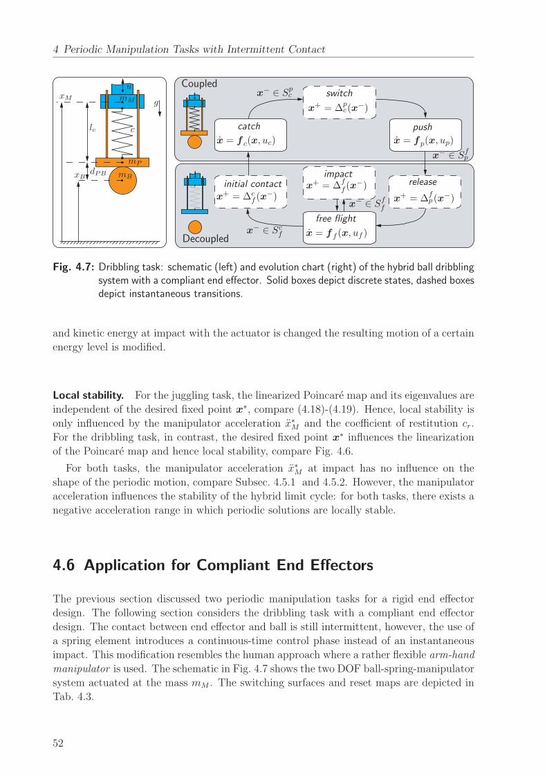
4 Periodic Manipulation Tasks with Intermittent Contact
mB
mM
mP
xM
xB
g
c
u
lc
dPB
switch
push
release
free flight
impactinitial contact
catch
x+ = ∆pc(x−)
x = fp(x, up)
x+ = ∆fp(x−)
x = ff (x, uf )
x+ = ∆ff (x
−)x+ = ∆c
f (x−)
x = f c(x, uc)
x− ∈ Sfp
x− ∈ Sff
x− ∈ Scf
x− ∈ Spc
Coupled
Decoupled
Fig. 4.7: Dribbling task: schematic (left) and evolution chart (right) of the hybrid ball dribblingsystem with a compliant end effector. Solid boxes depict discrete states, dashed boxesdepict instantaneous transitions.
and kinetic energy at impact with the actuator is changed the resulting motion of a certain
energy level is modified.
Local stability. For the juggling task, the linearized Poincare map and its eigenvalues are
independent of the desired fixed point x∗, compare (4.18)-(4.19). Hence, local stability is
only influenced by the manipulator acceleration x∗M and the coefficient of restitution cr.
For the dribbling task, in contrast, the desired fixed point x∗ influences the linearization
of the Poincare map and hence local stability, compare Fig. 4.6.
For both tasks, the manipulator acceleration x∗M at impact has no influence on the
shape of the periodic motion, compare Subsec. 4.5.1 and 4.5.2. However, the manipulator
acceleration influences the stability of the hybrid limit cycle: for both tasks, there exists a
negative acceleration range in which periodic solutions are locally stable.
4.6 Application for Compliant End Effectors
The previous section discussed two periodic manipulation tasks for a rigid end effector
design. The following section considers the dribbling task with a compliant end effector
design. The contact between end effector and ball is still intermittent, however, the use of
a spring element introduces a continuous-time control phase instead of an instantaneous
impact. This modification resembles the human approach where a rather flexible arm-hand
manipulator is used. The schematic in Fig. 4.7 shows the two DOF ball-spring-manipulator
system actuated at the mass mM . The switching surfaces and reset maps are depicted in
Tab. 4.3.
52

4.6 Application for Compliant End Effectors
Switching surface Reset map
Spc = xB x+ = ∆pc(x
−) = x−
Sfp = xM − xB − dPB − lc,0 x+ = ∆fp(x
−) = x−
Sff = xB − dB/2 x+ = ∆ff (x
−) = [1 1 1− cr]Tx−
Scf = xM − xB − dPB − lc,0 x+ = ∆cf (x
−) =
[
I3×3 03×1
0 0 mP
mB
mB
mB
]
x−
Tab. 4.3: Dribbling task with compliant end effector: switching surfaces and reset maps.
Coupled dynamics. When the ball is in contact with the plate, the system dynamics are
given by
mM xM = u− c (xM − xB − dPB − lc,0)−mMg
mBxB = c (xM − xB − dPB − lc,0)− mBg, (4.28)
where mB = mB + mP is the merged mass of ball and plate and g the gravitational
acceleration. The spring with stiffness c is restricted to its working range
lc = xM − xB − dPB, lc ∈ [lc,min, lc,0]. (4.29)
Decoupled dynamics. Here, it is assumed that manipulator and plate are rigidly con-
nected when the ball is not in contact with the plate. In practice, this can be realized by
an electro-mechanical lock. This assumption yields to the following free-flight dynamics
mM xM = u− mMg
xB = −g, (4.30)
where mM = mM +mP is the merged mass of manipulator and plate.
Hybrid dynamics. The cyclic ball dribbling task is of hybrid nature consisting of contin-
uous phases c (catch), p (push) and f (free flight) separated by instantaneous transitions.
The state of the system is given by
x =[
xM xB xM xB]T
(4.31)
and the dynamic model for phase i ∈ c, p, f is x = f i(x, ui). Here, phases p and c are
described by (4.28), and phase f is described by (4.30). Switching surfaces Sji determine
the occurrence of a transition from phase i to j, compare Sec. 2.2. The reset map for such
a transition can be written as
x+ = ∆ji
(
x−)
for x− ∈ Sji (4.32)
where x− is the state directly before the transition, x+ is the state directly after the
transition, and (i, j) ∈ (f, c), (c, p), (p, f), (f, f).
53
4 Periodic Manipulation Tasks with Intermittent Contact
The hybrid model of the complete system is given by
x = f i(x, ui) x− /∈ Sji
x+ = ∆ji
(
x−)
x− ∈ Sji (4.33)
with (i, j) ∈ (f, c), (c, p), (p, f), (f, f). A summary of discrete states and transitions for
a ball dribbling cycle is given in Tab. 4.3.
The ball dynamics between release and the subsequent initial contact are not directly
controlled. Hence, an algebraic relation for the state of the ball can be derived by inte-
grating (4.30). Furthermore, it is assumed that the manipulator dynamics are fast enough
to reach the desired state at initial contact, starting from release during the time that the
ball falls to the ground and bounces back. For the system analysis, it is reasonable to
consider only the controlled phase of the ball dribbling cycle involving the dynamics of the
underactuated ball-spring-manipulator system (4.28). The time from release to ground
impact is given by
tff − tfp =1
g
(
xB,p +√
x2B,p + 2g(xB,p − dB/2))
, (4.34)
where xB,p = xB(
tfp)
and xB,p = xB(
tfp)
. The ball velocity after the ground impact can
be described as function of the ball state at release or at initial contact :
x+B,f = xB
(
tf+f
)
= cr
√
x2B,p + 2g(xB,p − dB/2)
=√
(x−B,c)2 + 2g(x−B,c − dB/2), (4.35)
where x−B,c = xB(
tc−f)
and x−B,c = xB(
tc−f)
. Using (4.34) and (4.35), the evolution chart in
Fig. 4.7 can be modified by introducing a new mapping from release to initial contact.
Motion planning. During a dribbling cycle, there are two continuous phases that provide
control over the ball, namely catch and push. The desired continuous-time motion of
the ball-spring-manipulator system (4.28) can be described by the time evolution of its
generalized coordinates
xM = x∗M(t), xB = x∗B(t) , t ∈ [tb, te], tb < te. (4.36)
The facts that the dynamical system (4.28) is underactuated and the overall system (4.33)
is of hybrid nature pose a challenge for the planning of desired motions.
Virtual holonomic constraints. By introducing a set of geometric relations among the
general coordinates, the motion of (4.36) can be rewritten as
xM = φ1(θ), xB = φ2(θ) , θ = θ∗(t), t ∈ [tb, te] (4.37)
with a scalar variable θ ∈ [θb, θe] that is used as trajectory generator for parameterizing
the time evolution. Geometric functions among the generalized coordinates as introduced
54

4.6 Application for Compliant End Effectors
by (4.37) are known as virtual holonomic constraints, see Sec. 2.3. A convenient choice for
the system is the following:
[
xMxB
]
:= Φ(θ) =
[
φ(θ)
θ
]
. (4.38)
Suppose that there exists a control law u∗(t) for the input u that makes the virtual holo-
nomic constraint (4.38) invariant with respect to time. Then, the overall closed-loop system
can be generally represented by reduced order dynamics of the form [123]
α(θ)θ + β(θ)θ2 + γ(θ) = 0. (4.39)
The solutions of this virtually constrained system define achievable motions with precise
synchronization determined by (4.38). It means the whole motion is parameterized by the
evolution of the chosen configuration variable θ. The smooth coefficient functions of (4.39)
can be derived by substituting (4.38) into the system dynamics (4.28):
α(θ) = mB, β(θ) = 0, γ(θ) = −c (φ(θ)− θ − dPB − lc,0) + mBg. (4.40)
The reduced order dynamics of the form (4.39) is always integrable [123]. Specifically, the
integral function
I(θb, θb, θ, θ) = θ2 − θb2+
∫ θ
θb
2γ(s)
α(s)ds (4.41)
preserves its zero value along the solution of (4.39), initiated at [θb(tb), θb(tb)] = [θb, θb].
With the above arguments, the motion planning problem is converted from a search of
feasible orbits in the state space into a search for a parameterizing function φ(θ) such that
a desired solution of the reduced dynamics is found. Here, a Bezier polynomial
φ(θ) =M∑
k=0
ak
(
M
k
)
sk(1− s)M−k, s =θ − θbθe − θb
(4.42)
is used as geometric relation between the generalized coordinates [143]. Hence, one needs
to find the coefficients a = [a0 . . . aM ] that lead to the desired time evolution θ∗(t) between
the specified initial and final conditions [θb, θb] and [θe, θe].
Trajectory optimization. For the trajectory optimization, the following restrictions are
considered: at the beginning of the catching phase and at the end of the pushing phase, the
spring is constrained to be at equilibrium length. Furthermore, the condition of continuity
requires x+ = ∆pc(x
−) = x−. With these requirements, the Bezier coefficients a(c)0 , a
(p)0
and a(p)M are fixed. The remaining coefficients a(c) and a(p) of the Bezier polynomials for
the catching and the pushing phase are determined by an optimization. The nonlinear
55
4 Periodic Manipulation Tasks with Intermittent Contact
optimization problem is defined as
minγ∈Γ
Ji(γ)
with Γ =
γ ∈ R2M−1, ci(γ) ≤ 0, ce(γ) = 0
(4.43)
γ =[
a(c)1 . . . a
(c)M , a
(p)1 . . . a
(p)M−1
]
.
The inequality constraints ci(γ) originate from the limitations of the physical system,
such as maximum actuator acceleration and limits of the spring deflection. The equality
constraint ce(γ) ensures the validity of the reduced order dynamics:
ci(γ) =
||u(γ)|| − amax(xM(γ)− xB − dPB)− lc,0lc,min − (xM(γ)− xB − dPB)
, ce(γ) = I(θb, θb, θ, θ,γ). (4.44)
Two different cost functions are considered for the trajectory optimization. The function
J1 evaluates the maximum manipulator velocity and J2 estimates the energy consumption:
J1(γ) = λ max ||xM(t)||2 + e(te)
J2(γ) =λ
T
∫ te
tb
u(t)2dt+ e(te), (4.45)
with λ = 102, T = te − tb and the terminal cost
e(te) = λvev(te)2 + λpep(te)
2 (4.46)
which punishes deviations of the final velocity and position (λv = λp = 106) at the end of
each phase. Based on these cost functions, trajectory optimization has been performed for
different degrees of the Bezier polynomial (4.42). For the optimization results, a particular
ball dribbling cycle is considered: the desired dribbling height is set to hd = x−B,c =
x+B,p = 0.9 m, the initial contact to [x+B,c, x+B,c] = [0.8 m, 1.72 m/s] and the release to
x−B,p = x+B,f = 0.5 m is considered. With a known coefficient of restitution cr, the ball
velocity x−B,p at release is determined with (4.35). Table 4.4 summarizes the results of
the numerical optimization. For both cost functions, the higher order Bezier polynomials
naturally lead to reduced costs. However, there is no significant difference in the costs
betweenM = 5 andM = 6. Hence, a Bezier polynomial of orderM = 5 is a good trade-off
between cost optimality and numerical complexity, which is relevant for the implementation
on the real system. For comparison, Fig. 4.8 shows optimized trajectories and the resulting
spring deflection for M = 3 and M = 5 obtained when using J1.
Control design: transverse linearization. Given the desired orbit obtained through
the optimization process, the next step is to design a controller that stabilizes the ball-
spring-manipulator system in the vicinity of the desired limit cycle. Based on the system
description in the form of (4.37), new coordinates and velocities are introduced in the
56

4.6 Application for Compliant End Effectors
0 0.1 0.2 0.30.4
0.6
0.8
1
1.2
1.4
t [s]
posi
tions
xB
,x
M[m
]
xB , M = 3
xM , M = 3
xB , M = 5
xM , M = 5
switch, M=3switch, M=5
(a) positions xB , xM
0 0.1 0.2 0.3−6
−4
−2
0
2
t [s]
velo
citi
esx
B,x
M[m
/s]
xB, M = 3xM , M = 3xB, M = 5xM , M = 5
switch, M=5
switch, M=3
(b) velocities xB , xM
0 0.1 0.2 0.3−0.08
−0.06
−0.04
−0.02
0
t [s]
spri
ng
defl
ecti
on
[m]
M = 3M = 5
switch, M=3
switch, M=5
(c) spring deflection
0.5 0.6 0.7 0.8 0.90.8
0.9
1
1.1
1.2
1.3
position xB [m]
posi
tion
xM
[m]
M = 3M = 5
catch
push
(d) virtual holonomic constraints
Fig. 4.8: Optimized trajectories for different Bezier degrees using cost function J1. The solidlines indicate the switch from catch to push phase.
Cost function Bezier degree
3 4 5 6
J1 779 720 708 706
J2 80249 77663 75234 74134
Tab. 4.4: Costs of the optimized trajectories for different Bezier degrees.
57
4 Periodic Manipulation Tasks with Intermittent Contact
vicinity of the target orbit:
xM = φ(θ) + y, xB = θ
xM = φ′
(θ)θ + y, xB = θ. (4.47)
The dynamics of the synchronization error y to the specified virtual holonomic constraint
can be computed from the system dynamics (4.28) by substituting (4.47):
y = r(θ, θ, y, y) + (1/mM) u = v. (4.48)
An auxiliary control signal v is introduced by a control transformation via partial feedback
linearization [131]. The dynamics of θ is given by substituting (4.47) into the second order
differential equation (4.39), which yields
mB θ − c (φ(θ)− θ − dPB − lc,0) + mBg = −cy, (4.49)
where the right hand side equals to zero on the desired orbit. The target motion (4.36) in
the new generalized coordinates is given by
y∗(t) ≡ 0, θ = θ∗(t) , t ∈ [tb, te]. (4.50)
The dynamic system has a natural choice of transverse coordinates
x⊥ =[
I(θ, θ, θ∗b , θ∗b ) y y
]T, (4.51)
that describe the system’s behavior away from a specified orbit [123]. A transverse lin-
earization along a continuous-time target motion (4.50) can be analytically computed to
be used for system analysis and control design:
z = A(t)z + bv =
0 2θ∗(t)mB
c 0
0 0 1
0 0 0
I
Y1Y2
+
0
0
1
v, (4.52)
where z =[
I Y1 Y2]T
denotes the linearization for x⊥. A cyclic solution z = z(t) =
z(t+ T ) with time period T = tfp − tcf and a switch at ts = tpc is defined by
z = A(s)z + bv, s = t mod T
A(s) =
Ac(s), s ∈ (0, ts]
Ap(s), s ∈ (ts, T )(4.53)
z(t+k ) = f ri(
z(t−k ))
, tk = kT, k ∈ N.
The operator f ri is the mapping from release to initial contact based on (4.35).
58
4.7 Summary
Closed-loop system. Consider the control law
v = k(s)z, k(s) =
kc(s), s ∈ (0, ts]
kp(s), s ∈ (ts, T )(4.54)
for the hybrid linear system (4.53). It can be shown that exponential stability of the
origin for the linear impulsive system is equivalent to exponential orbital stability of the
periodic motion for the nonlinear one [124]. For reasons of implementation, only a constant
feedback of the synchronization error xM − φ(xB) is used since these measurements are
available:
kc =[
0 kc2 0]
, kp =[
0 kp2 0]
. (4.55)
In addition to the control during the two contact phases catch and push, a control for the
manipulator during the non-contact phase has to be applied. This control law must ensure
that the manipulator is at the desired state when the controlled phase of the ball dribbling
cycle starts, compare Subsec. 6.4.2.
4.7 Summary
The chapter discussed periodic manipulation tasks with intermittent contact. In Sec-
tion 4.1, an overview on related work was given and the challenges of the trajectory plan-
ning were addressed in Section 4.2. Next, methods for the stability analysis of periodic
solutions of (hybrid) dynamical systems were outlined in Sections 4.3 and 4.4. Then, two
applications for rigid end effectors were presented in Section 4.5. First, the classic juggling
task was studied: the section reviewed the control strategies proposed in the literature and
presented a new approach for optimal trajectory planning based on a non-local stability
analysis. Ball dribbling was introduced as novel case study for dynamic dexterity. The
system dynamics and optimal trajectory planning were discussed. A comparison with the
classic juggling task showed that the dribbling task is more challenging due to the oc-
currence of an additional, autonomous impact. In addition to dribbling with a rigid end
effector, a novel approach for the stabilization of human-like periodic ball dribbling motion
was presented in Section 4.6. Adding an elastic element to the manipulator promises two
benefits: first, the ball can be controlled in a continuous-time phase instead of an intermit-
tent contact. Second, impacts between manipulator and ball are avoided which reduces the
mechanical load. The virtual holonomic constraints approach was used to plan optimal
catching and pushing trajectories considering two different cost functions. An orbitally
stabilizing feedback controller was designed for the underactuated ball-spring-manipulator
system based on a transverse linearization along the desired motion.
59

4 Periodic Manipulation Tasks with Intermittent Contact
60
5 Perception and Interaction Control for
Dynamic Manipulation
Summary This chapter addresses the particular challenges that arise for the closed-loop
control of dynamic manipulation tasks and presents an extensive control structure to over-
come these challenges. Four different observer designs are developed to reconstruct the
forces/torques that are exchanged between the manipulator and its environment during
dynamic motions. The designs are evaluated in a simulation scenario as well as an exper-
iment. The force/torque observer is then integrated in a direct force control scheme to
improve the interaction control for dynamic manipulation tasks. Finally, an approach for
high-speed image processing is presented which allows to track and to predict the state of
objects during non-contact phases with high sampling rates.
The two previous chapters discussed trajectory planning and control strategies for dy-
namic manipulation tasks. It was shown that the successful execution of these tasks
generally requires some amount of sensory feedback. Clearly, state feedback is also needed
when performing conventional manipulation tasks. However, the dynamic nature of the
tasks studied in this work poses some additional challenges which have to be overcome.
The chapter addresses these challenges and the obtained results are prerequisites for the
experiments presented in Chapter 6.
In principle, feedback can be provided either at discrete times or continuously through-
out the task execution. During non-contact phases, the most valuable source of feedback is
visual information. When the manipulator is in contact with the environment, force/torque
measurements are another essential source of information. Like visual feedback, they al-
low to determine the pose of the manipulated object. Additionally, the measured forces
and torques also provide information about the acceleration of the object. This informa-
tion, however, is not directly accessible since the force/torque measurements are disturbed
by inertial and gravitational forces and measurement noise. For dynamic motions, this
is particularly a problem, since the tool inertia has here a non-negligible effect on the
measurements of the wrist F/T-sensor. Due to this fact, the chapter discusses observer
designs which allow the reconstruction of the forces and torques exchanged between the
manipulator and the environment.
Accurate knowledge of these contact forces improves the performance of the applied
interaction control scheme (direct or indirect force control). In addition to this sensory
information, a precise underlying motion control of the robot is a prerequisite for successful
61
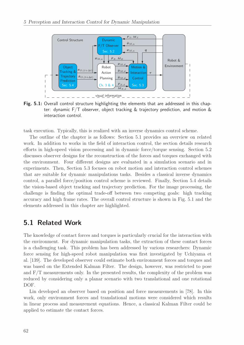
5 Perception and Interaction Control for Dynamic Manipulation
Robot &
Environment
Dynamic
F/T Observer
Object
Tracking &
Trajectory
Prediction
Robot
Action
Planning
Motion &
Interaction
Control
Sec. 5.2
Ch. 3 & 4 Sec. 5.3Sec. 5.4
Control Structure
visual information
xO,(t+∆t)
xO,(t+∆t)
xM,d
xM,d
xM,d
τ
FS , MS
FE , ME
FE,d
ME,d
q
xM,a
xM,a
xM,a
Fig. 5.1: Overall control structure highlighting the elements that are addressed in this chap-ter: dynamic F/T observer, object tracking & trajectory prediction, and motion &interaction control.
task execution. Typically, this is realized with an inverse dynamics control scheme.
The outline of the chapter is as follows: Section 5.1 provides an overview on related
work. In addition to works in the field of interaction control, the section details research
efforts in high-speed vision processing and in dynamic force/torque sensing. Section 5.2
discusses observer designs for the reconstruction of the forces and torques exchanged with
the environment. Four different designs are evaluated in a simulation scenario and in
experiments. Then, Section 5.3 focuses on robot motion and interaction control schemes
that are suitable for dynamic manipulations tasks. Besides a classical inverse dynamics
control, a parallel force/position control scheme is reviewed. Finally, Section 5.4 details
the vision-based object tracking and trajectory prediction. For the image processing, the
challenge is finding the optimal trade-off between two competing goals: high tracking
accuracy and high frame rates. The overall control structure is shown in Fig. 5.1 and the
elements addressed in this chapter are highlighted.
5.1 Related Work
The knowledge of contact forces and torques is particularly crucial for the interaction with
the environment. For dynamic manipulation tasks, the extraction of these contact forces
is a challenging task. This problem has been addressed by various researchers: Dynamic
force sensing for high-speed robot manipulation was first investigated by Uchiyama et
al. [139]. The developed observer could estimate both environment forces and torques and
was based on the Extended Kalman Filter. The design, however, was restricted to pose
and F/T measurements only. In the presented results, the complexity of the problem was
reduced by considering only a planar scenario with two translational and one rotational
DOF.
Lin developed an observer based on position and force measurements in [78]. In this
work, only environment forces and translational motions were considered which results
in linear process and measurement equations. Hence, a classical Kalman Filter could be
applied to estimate the contact forces.
62
5.1 Related Work
Garcia et al. investigated a sensor fusion approach for dynamic force/torque estima-
tion [42, 43]. In addition to pose and F/T measurements, an inertial sensor was used to
measure the tool acceleration. In the EKF-based observer design, the environment forces
and torques were not considered. The estimation error was utilized to obtain a contact
F/T estimator with low-pass properties. Considering the nonlinear process model for the
torques, it seems problematic to use the estimation error of such an observer to determine
the environment torques. In addition, the representation of the tool orientation with Euler
angles appears critical because of the well-known issues with representation singularities.
Kroger et al. also discussed a fusion of F/T and acceleration information for contact
force/torque estimation [74]. In their work, characteristic properties of F/T and acceler-
ation sensors were reported [75]. Furthermore, translational and rotational acceleration
estimates based on pose measurements were derived. However, the calculation of con-
tact forces and torques was performed without considering the stochastic properties of the
signals, hence limiting the effectiveness of the approach.
For dynamic manipulation tasks, the precise timing and execution of motions are pre-
liminary requirements. Inverse dynamics control schemes are a well-established method
for improved motion control [126, 125, 94]. Friction compensation is an essential part of
the inverse dynamics control. Due to the various friction phenomena that need to be con-
sidered, this is a challenging task (compare Sec. 2.5). Surveys on friction compensation
for robotic manipulators were provided by Olsson and Bona [96, 97, 14]. Detailed exper-
imental results on friction compensation for the dual-arm robot used in this work have
been presented by Ueberle [140]. Comprehensive discussions on motion control for robotic
manipulators were presented by Siciliano and Khatib [126, 125].
In addition to precise motion execution, dynamic manipulation tasks also require in-
teraction with the environment. Hence, an interaction control is needed in addition to
pure motion control. Numerous strategies for such an interaction control have been pro-
posed in literature: in general, these interaction control schemes can be classified into
direct and indirect force control. The former approach, which includes impedance and
admittance control, was first proposed by Hogan [53]. A drawback of indirect force control
schemes is the fact that the contact forces/torques at the end effector can not be directly
controlled. This shortcoming is addressed by direct force control, which allows to con-
trol the forces/torques that are exchanged between end effector and environment. Direct
force control was first proposed by Raibert and Craig and later extended by Yoshikawa
and Khatib to include an inverse dynamics motion control [101, 149, 70]. These hybrid
force/position control schemes use a task-specific selection matrix that determines for each
task coordinate whether it is force or position controlled. This is a drawback as the struc-
ture of the control has to be changed during task execution. The problem was addressed
by Chiaverini and Sciavicco, who presented a parallel approach to force/position control
of robotic manipulators [28]. Here, the position and force controller act in parallel, and
conflicting situations are resolved by assigning a higher priority to the force control. The
approach was extended by Natale for interaction control of six DOF tasks [94]. A compre-
hensive survey on interaction control schemes including experimental results was presented
by Chiaverini et al. and Natale [29, 94]. For the intended applications in this thesis, the
parallel approach is best suited as it offers both direct force control and relatively high
63
5 Perception and Interaction Control for Dynamic Manipulation
structural flexibility.
Rizzi and Koditschek were the first who emphasized the importance of visual attention
control for dynamically dexterous robots [106]. In order to achieve higher frame rates,
they proposed to reduce the search window on the images obtained from the camera sys-
tem. High-speed vision improves control performance in vision-based control due to higher
frame rates and lower latencies. Recent progress in sensors, bus systems and semiconduc-
tor technology has led to a few works on vision with more than 30 Hz frame rate during
the last decade: Ishikawa et al. have developed high-speed vision systems with various res-
olutions and fast low-level image processing functions integrated on customized processing
hardware allowing framerates of up to 1 kHz. These vision systems were applied to various
dynamic vision-based manipulation tasks, e.g. ball dribbling with multi-fingered hands,
ball catching, ball batting, and regrasping [122, 59, 119, 39]. In the field of visual servo
control, a number of works with higher framerates (> 30 Hz) exist, see e.g. [93, 41, 146].
5.2 Dynamic Contact Force/Torque Observer
For robots that are destined to leave the classical industrial settings, one major challenge
is the physical interaction with unknown and/or changing environments. Such an interac-
tion requires knowledge of the exchanged contact forces and torques. To this end, robotic
systems nowadays are typically equipped with force/torque sensors at the wrist. By using
force control schemes that rely on measurements from these sensors, conventional ma-
nipulation tasks are successfully executed. In particular for dynamic manipulation tasks,
however, the problem arises that the inertial forces/torques of the end effector have a non-
negligible effect on the measurements of the wrist sensor. This does not only degrade the
performance of the interaction control but also constitutes a safety risk.
The section discusses four different contact force/torque observer designs to overcome
this problem: two approaches are based on the Extended Kalman Filter (EKF) and two
approaches are based on the Unscented Kalman Filter (UKF). For each case, two differ-
ent measurement vectors are considered: the first one only uses pose and force/torque
measurements, whereas the second one also uses acceleration measurements to determine
the contact forces and torques. The four observer designs are evaluated in simulation and
experiment for six degrees-of-freedom tasks, paying particular attention to the influence of
changing operating conditions.
Fig. 5.2 illustrates the typical hardware setup with a F/T-sensor located at the wrist.
For dynamic motions, the inertial forces/torques of the end effector have a non-negligible
effect on the force sensor measurements. Hence, the measurements do not correspond to
the actual environmental interaction forces/torques. In general, the measured forces F S
and torques MS are constituted by the following components
[
F S(t)
MS(t)
]
=
[
F E(t)
ME(t)
]
+
[
F I(t)
M I(t)
]
+
[
FG(t)
MG(t)
]
(5.1)
where F E and ME are the environmental contact forces and torques, F I and M I are the
inertial forces and torques, and FG and MG are the forces and torques due to gravity.
64
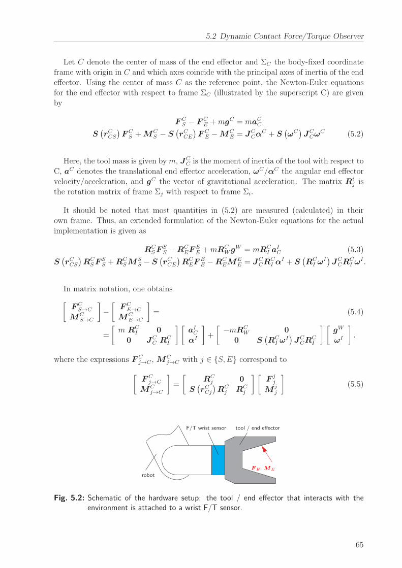
5.2 Dynamic Contact Force/Torque Observer
Let C denote the center of mass of the end effector and ΣC the body-fixed coordinate
frame with origin in C and which axes coincide with the principal axes of inertia of the end
effector. Using the center of mass C as the reference point, the Newton-Euler equations
for the end effector with respect to frame ΣC (illustrated by the superscript C) are given
by
F CS − F C
E +mgC = maCC
S(
rCCS)
F CS +MC
S − S(
rCCE)
F CE −MC
E = JCCα
C + S(
ωC)
JCCω
C (5.2)
Here, the tool mass is given bym, JCC is the moment of inertia of the tool with respect to
C, aC denotes the translational end effector acceleration, ωC/αC the angular end effector
velocity/acceleration, and gC the vector of gravitational acceleration. The matrix Rij is
the rotation matrix of frame Σj with respect to frame Σi.
It should be noted that most quantities in (5.2) are measured (calculated) in their
own frame. Thus, an extended formulation of the Newton-Euler equations for the actual
implementation is given as
RCSF
SS −RC
EFEE +mRC
WgW = mRCI a
IC (5.3)
S(
rCCS)
RCSF
SS +RC
SMSS − S
(
rCCE)
RCEF
EE −RC
EMEE = JC
CRCI α
I + S(
RCI ω
I)
JCCR
CI ω
I .
In matrix notation, one obtains
[
F CS→C
MCS→C
]
−
[
F CE→C
MCE→C
]
= (5.4)
=
[
m RCI 0
0 JCC RC
I
] [
aICαI
]
+
[
−mRCW 0
0 S(
RCI ω
I)
JCCR
CI
] [
gW
ωI
]
.
where the expressions F Cj→C , M
Cj→C with j ∈ S,E correspond to
[
F Cj→C
MCj→C
]
=
[
RCj 0
S(
rCCj)
RCj RC
j
] [
Fjj
Mjj
]
(5.5)
F/T wrist sensor tool / end effector
robot
FE , ME
Fig. 5.2: Schematic of the hardware setup: the tool / end effector that interacts with theenvironment is attached to a wrist F/T sensor.
65

5 Perception and Interaction Control for Dynamic Manipulation
ΣW
ΣS
ΣC
ΣE
p
rCS
rCE
ME
MS
F S
FE
m, JC
inertial frame
Fig. 5.3: Forces and moments applied at the end effector
5.2.1 Continuous-Time System Model
In the following, all quantities are expressed in frame C and in order to facilitate the
notation, the superscript C is omitted. However, velocities and acceleration are, of course,
absolute quantities calculated with respect to the inertial frame and only expressed in
frame C. Let
x(t) = x =[
pT oT vT ωT F TS MT
S F TE MT
E
]T∈ R
25 (5.6)
denote the state vector of the system. Here, p and o are the position and orientation
(in quaternion) of the tools center of mass with respect to the inertial frame and v is the
(absolute) translational tool velocity. For the observer design, two different measurement
vectors
y1(t) = y1 =[
pT oT F TS MT
S
]T∈ R
13 (5.7)
y2(t) = y2 =[
pT oT F TS MT
S aT αT ωT]T
∈ R22
are considered. While y1 relies solely on position and force/torque measurements, y2 also
includes acceleration and (rotational) velocity measurements. As proposed by [139], it is
assumed that the process model for the sensor and environment forces and torques can
be approximated by a white and Gaussian process. Based on (5.4)-(5.7), the nonlinear,
continuous-time system model
x = f(x,w)
yi = hi(x,ν) (5.8)
66
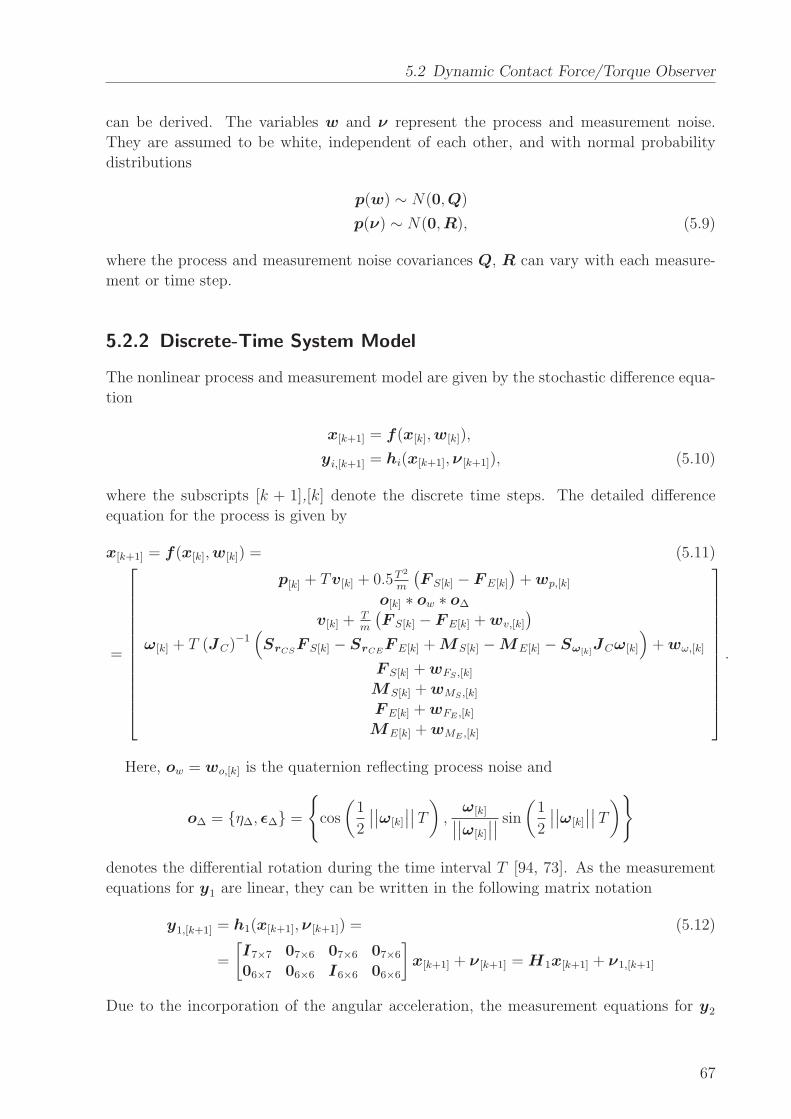
5.2 Dynamic Contact Force/Torque Observer
can be derived. The variables w and ν represent the process and measurement noise.
They are assumed to be white, independent of each other, and with normal probability
distributions
p(w) ∼ N(0,Q)
p(ν) ∼ N(0,R), (5.9)
where the process and measurement noise covariances Q, R can vary with each measure-
ment or time step.
5.2.2 Discrete-Time System Model
The nonlinear process and measurement model are given by the stochastic difference equa-
tion
x[k+1] = f(x[k],w[k]),
yi,[k+1] = hi(x[k+1],ν [k+1]), (5.10)
where the subscripts [k + 1],[k] denote the discrete time steps. The detailed difference
equation for the process is given by
x[k+1] = f(x[k],w[k]) = (5.11)
=
p[k] + Tv[k] + 0.5T2
m
(
F S[k] − F E[k]
)
+wp,[k]
o[k] ∗ ow ∗ o∆
v[k] +Tm
(
F S[k] − F E[k] +wv,[k]
)
ω[k] + T (JC)−1(
SrCSF S[k] − SrCE
F E[k] +MS[k] −ME[k] − Sω[k]JCω[k]
)
+wω,[k]
F S[k] +wFS ,[k]
MS[k] +wMS ,[k]
F E[k] +wFE ,[k]
ME[k] +wME ,[k]
.
Here, ow = wo,[k] is the quaternion reflecting process noise and
o∆ = η∆, ǫ∆ =
cos
(
1
2
∣
∣
∣
∣ω[k]
∣
∣
∣
∣T
)
,ω[k]∣
∣
∣
∣ω[k]
∣
∣
∣
∣
sin
(
1
2
∣
∣
∣
∣ω[k]
∣
∣
∣
∣T
)
denotes the differential rotation during the time interval T [94, 73]. As the measurement
equations for y1 are linear, they can be written in the following matrix notation
y1,[k+1] = h1(x[k+1],ν [k+1]) = (5.12)
=
[
I7×7 07×6 07×6 07×6
06×7 06×6 I6×6 06×6
]
x[k+1] + ν [k+1] = H1x[k+1] + ν1,[k+1]
Due to the incorporation of the angular acceleration, the measurement equations for y2
67
5 Perception and Interaction Control for Dynamic Manipulation
are nonlinear:
y2,[k+1] = h2(x[k+1],ν [k+1]) = (5.13)
=
H1x[k+1] + ν1,[k+1]1m
(
F S[k+1] − F E[k+1]
)
+ νa,[k+1]
J−1C
(
MS[k+1] −ME[k+1] − Sω[k+1]JCω[k+1] + SrCS
F S[k+1] − SrCEF E[k+1]
)
+ να,[k+1]
ω[k+1] + νω,[k+1]
.
5.2.3 Filter Design
As shown in (5.11), the system is characterized by a nonlinear process model. In addition,
the measurement model for y2 is also nonlinear, compare (5.13). Hence, a nonlinear filter
design is needed for the six DOF dynamic F/T observer. In the following, two different
approaches for nonlinear systems are evaluated: Extended Kalman Filter and Unscented
Kalman Filter.
Extended Kalman Filter (EKF). The EKF extends the Kalman Filter for nonlinear
systems by linearizing about the current mean and covariance and can hence be applied to
the given nonlinear estimation problem [142]. Using the following notations for the partial
derivatives,
A[k] =∂f(x[k−1],0)
∂xW [k] =
∂f(x[k−1],0)
∂w
H i,[k] =∂hi(x[k−1],0)
∂xV i,[k] =
∂hi(x[k−1],0)
∂ν, (5.14)
the EKF time update equations are given by
x−[k] = f(x−
[k−1],0)
P−[k] = A[k]P [k−1]A
T[k] +W [k]Q[k−1]W
T[k]. (5.15)
The equations in (5.15) predict the state x[k] and the error covariance P [k] at time step k
based on the results from the previous time step k − 1.
Then, the EKF measurement update equations are used to correct these predictions
based on the actual measurements at time step k, compare (5.16).
K [k] = P−[k]H
Ti,[k]
(
H i,[k]P−[k]H
Ti,[k] + V i,[k]R[k]V
Ti,[k]
)−1
x[k] = x−[k] +K [k]
(
yi,[k] − hi(x−[k],0)
)
(5.16)
P [k] = (I25×25 −K [k]H i,[k])P−[k].
The first equation computes the Kalman gain K [k], the second equation updates the
estimate x[k] with the current measurement yi,[k] and the third equation updates the error
covariance P [k].
68

5.2 Dynamic Contact Force/Torque Observer
Unscented Kalman Filter (UKF). As detailed in the previous paragraph, the EKF ap-
proximates the state distribution by a Gaussian random variable, which is then propagated
through the first-order linearization of the nonlinear system. This can introduce large er-
rors in the mean and covariance, particularly if the system is highly nonlinear on the
considered time scale.
The UKF is based on the intuition that, when having a fixed number of parameters,
it is easier to approximate a Gaussian distribution than it is to approximate an arbitrary
nonlinear function [66]. Hence, instead of a linearization, the UKF uses a set of determin-
istic sample points (sigma points) to parameterize the mean and the covariance. The state
distribution is still approximated by a Gaussian random variable, but is now represented
through the set of sigma points. The sample points capture the true mean and covariance
of the Gaussian random variable. The sigma points are then propagated through the actual
nonlinear system (and not through a linearization). They capture the posterior mean and
covariance accurately to the third order whereas with the EKF, only first order accuracy
is achieved [141]. In addition to the higher accuracy, the UKF can be applied to a broader
class of system since it does not require the calculation of partial derivatives. In contrast to
particle filters, the UKF selects the sample points in a deterministic way. Hence, compared
to e.g. Monte Carlo methods, less sample points are needed. The UKF belongs to the
class of so called Sigma Point Kalman Filters (SPKF), together with Central Difference
Kalman filter (CDKF), Square-Root SPKF and SPKF smoother [141]. In the following,
the basic algorithm of the UKF is summarized - for the detailed idea and implementation
notes of the filter, see [64, 65].
For a state vector x of dimension L, the 2L + 1 sigma points (vectors) χi and their
corresponding weights for the covariance G(c)i and the mean G
(m)i are created according to
the following procedure
χ0 = x[k]
χi =
x[k] +(√
(L+ λ)P [k]
)
ifor i = 1, . . . , L
x[k] −(√
(L+ λ)P [k]
)
i−Lfor i = L+ 1, . . . , 2L
(5.17)
G(c)0 =
λ
L+ λ+(
1− α2 + β)
G(m)0 =
λ
L+ λ
G(c)i = G
(m)i =
1
2 (L+ λ)for i = 1, . . . , 2L
with λ = α2(L+ κ)− L
L = dim (x)
where P [k] is the covariance matrix of x[k] and(√
(L+ λ)P [k]
)
ithe i-th column of the
matrix square root. The parameters α and κ define the distribution of the sigma points
around the mean and are typically set to small positive values. The parameter β is used to
include prior knowledge on the distribution of x[k]. For Gaussian distributions, the optimal
choice is β = 2 [141]. For the UKF-based observers in this work, the parameters are set
to α = 10−3, κ = 0, and β = 2.
With the sigma points and the corresponding weights defined in (5.17), the basic for-
69

5 Perception and Interaction Control for Dynamic Manipulation
mulation of the UKF is as follows: in the first step, sigma points for the augmented state
vector xa[k−1] =[
x[k−1] w[k−1] ν [k−1]
]Tand the corresponding augmented covariance ma-
trix P a[k−1] = diag
([
P [k−1] Q R])
are calculated, leading to
χai,[k−1] =
[
χxi,[k−1] χw
i,[k−1] χνi,[k−1]
]T
. (5.18)
Next, the sigma points are propagated through process and measurement model
χxi,[k] = f
(
χxi,[k−1],χ
wi,[k−1]
)
Y i,[k] = h(
χxi,[k−1],χ
νi,[k−1]
)
for i = 0, . . . , 2L. (5.19)
The time update equations (prediction) are then given by
x−[k] =
2L∑
i=0
G(m)i χx
i,[k]
P−[k] =
2L∑
i=0
G(c)i
[
χxi,[k] − x−
[k]
] [
χxi,[k] − x−
[k]
]T
(5.20)
y−[k] =
2L∑
i=0
G(m)i Y i,[k].
The measurement update equations (correction step) are
K [k] = P xy,[k]P−1yy,[k]
x[k] = x−[k] +K [k]
(
yi,[k] − y−[k]
)
(5.21)
P [k] = P−[k] −K [k]P yy,[k]K
T[k],
with P yy,[k] =2L∑
i=0
G(c)i
[
Y i,[k] − y−[k]
] [
Y i,[k] − y−[k]
]T
P xy,[k] =2L∑
i=0
G(c)i
[
χxi,[k] − x−
[k]
] [
Y i,[k] − y−[k]
]T
.
In contrast to the EKF, the UKF does not require analytical derivatives, compare (5.14).
The computational complexity of EKF and UKF is comparable [141].
5.2.4 Simulation
The purpose of the following simulation study is the evaluation of the four observer designs
(EKF with y1, EKF with y2, UKF with y1, UKF with y2). Particularly, the simulation
of the system facilitates the investigation of the observer performance for changing envi-
ronment conditions. In the following, this will be denoted as scenario I.
While gravity has a significant effect on the measured forces and torques, the compen-
sation is relatively easy as its influence is only configuration-dependent. In contrast, the
compensation of inertial effects is more challenging since these forces/torques also depend
70
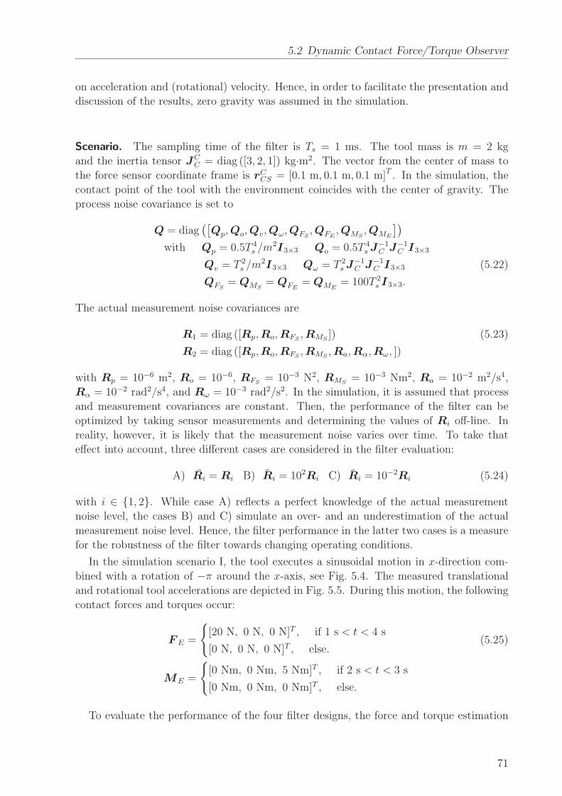
5.2 Dynamic Contact Force/Torque Observer
on acceleration and (rotational) velocity. Hence, in order to facilitate the presentation and
discussion of the results, zero gravity was assumed in the simulation.
Scenario. The sampling time of the filter is Ts = 1 ms. The tool mass is m = 2 kg
and the inertia tensor JCC = diag ([3, 2, 1]) kg·m2. The vector from the center of mass to
the force sensor coordinate frame is rCCS = [0.1 m, 0.1 m, 0.1 m]T . In the simulation, the
contact point of the tool with the environment coincides with the center of gravity. The
process noise covariance is set to
Q = diag([
Qp,Qo,Qv,Qω,QFS,QFE
,QMS,QME
])
with Qp = 0.5T 4s /m
2I3×3 Qo = 0.5T 4s J
−1C J−1
C I3×3
Qv = T 2s /m
2I3×3 Qω = T 2s J
−1C J−1
C I3×3 (5.22)
QFS= QMS
= QFE= QME
= 100T 2s I3×3.
The actual measurement noise covariances are
R1 = diag ([Rp,Ro,RFS,RMS
]) (5.23)
R2 = diag ([Rp,Ro,RFS,RMS
,Ra,Rα,Rω, ])
with Rp = 10−6 m2, Ro = 10−6, RFS= 10−3 N2, RMS
= 10−3 Nm2, Ra = 10−2 m2/s4,
Rα = 10−2 rad2/s4, and Rω = 10−3 rad2/s2. In the simulation, it is assumed that process
and measurement covariances are constant. Then, the performance of the filter can be
optimized by taking sensor measurements and determining the values of Ri off-line. In
reality, however, it is likely that the measurement noise varies over time. To take that
effect into account, three different cases are considered in the filter evaluation:
A) Ri = Ri B) Ri = 102Ri C) Ri = 10−2Ri (5.24)
with i ∈ 1, 2. While case A) reflects a perfect knowledge of the actual measurement
noise level, the cases B) and C) simulate an over- and an underestimation of the actual
measurement noise level. Hence, the filter performance in the latter two cases is a measure
for the robustness of the filter towards changing operating conditions.
In the simulation scenario I, the tool executes a sinusoidal motion in x-direction com-
bined with a rotation of −π around the x-axis, see Fig. 5.4. The measured translational
and rotational tool accelerations are depicted in Fig. 5.5. During this motion, the following
contact forces and torques occur:
F E =
[20 N, 0 N, 0 N]T , if 1 s < t < 4 s
[0 N, 0 N, 0 N]T , else.(5.25)
ME =
[0 Nm, 0 Nm, 5 Nm]T , if 2 s < t < 3 s
[0 Nm, 0 Nm, 0 Nm]T , else.
To evaluate the performance of the four filter designs, the force and torque estimation
71
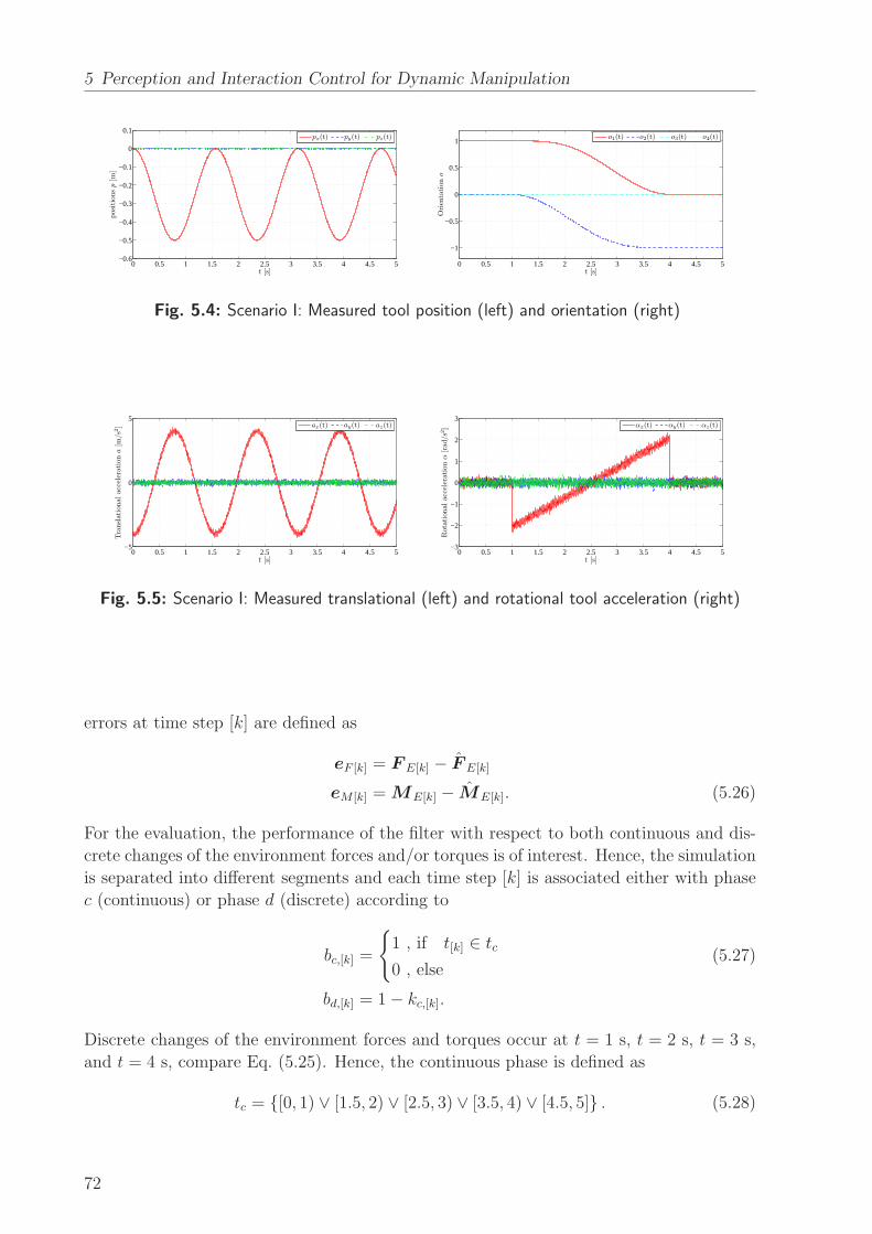
5 Perception and Interaction Control for Dynamic Manipulation
0 0.5 1 1.5 2 2.5 3 3.5 4 4.5 5−0.6
−0.5
−0.4
−0.3
−0.2
−0.1
0
0.1
t [s]
pos
itio
ns
p[m
]
px(t) py(t) pz(t)
0 0.5 1 1.5 2 2.5 3 3.5 4 4.5 5
−1
−0.5
0
0.5
1
t [s]
Ori
enta
tion
o
o1(t) o2(t) o3(t) o4(t)
Fig. 5.4: Scenario I: Measured tool position (left) and orientation (right)
0 0.5 1 1.5 2 2.5 3 3.5 4 4.5 5−5
0
5
t [s]
Tra
nsl
atio
nal
acce
lera
tion
a[m
/s2]
ax(t) ay(t) az(t)
0 0.5 1 1.5 2 2.5 3 3.5 4 4.5 5−3
−2
−1
0
1
2
3
t [s]
Rot
atio
nal
acce
lera
tion
α[r
ad/s
2]
αx(t) αy(t) αz(t)
Fig. 5.5: Scenario I: Measured translational (left) and rotational tool acceleration (right)
errors at time step [k] are defined as
eF [k] = F E[k] − F E[k]
eM [k] = ME[k] − ME[k]. (5.26)
For the evaluation, the performance of the filter with respect to both continuous and dis-
crete changes of the environment forces and/or torques is of interest. Hence, the simulation
is separated into different segments and each time step [k] is associated either with phase
c (continuous) or phase d (discrete) according to
bc,[k] =
1 , if t[k] ∈ tc
0 , else(5.27)
bd,[k] = 1− kc,[k].
Discrete changes of the environment forces and torques occur at t = 1 s, t = 2 s, t = 3 s,
and t = 4 s, compare Eq. (5.25). Hence, the continuous phase is defined as
tc = [0, 1) ∨ [1.5, 2) ∨ [2.5, 3) ∨ [3.5, 4) ∨ [4.5, 5] . (5.28)
72

5.2 Dynamic Contact Force/Torque Observer
With (5.26)-(5.28), the scalar error measures
eF,c =N∑
k=1
Tsbc,[k]∣
∣
∣
∣eF [k]
∣
∣
∣
∣ eF,d =N∑
k=1
Tsbd,[k]∣
∣
∣
∣eF [k]
∣
∣
∣
∣
eM,c =N∑
k=1
Tsbc,[k]∣
∣
∣
∣eM [k]
∣
∣
∣
∣ eM,d =N∑
k=1
Tsbd,[k]∣
∣
∣
∣eM [k]
∣
∣
∣
∣ (5.29)
are defined. In addition, the error measures
eF,Σ = eF,c + eF,d and eM,Σ = eM,c + eM,d (5.30)
are used to evaluate the combined performance in phases c and d.
Results. For case A), the measured sensor force, the true environment force, and the
estimated environment force (UKF with y2) in x-direction are depicted in Fig. 5.6(a). The
force estimation errors for the four different filter designs are illustrated in Fig. 5.6(c). The
forces along y- and z-axis are not displayed since no environment forces were applied in this
direction. But they are, of course, considered in the calculation of the error measures. The
measured sensor torques, the true environment torques, and the estimated environment
torques (UKF with y2) around the three axis are depicted in Fig. 5.6(b), 5.6(e), and 5.6(f).
The corresponding estimation errors for the four filters are shown in Fig. 5.6(d), 5.6(g),
and 5.6(h). It should be noted that all three measured torques show significant deviations
from zero, despite the fact that an environment torque is only applied around the z-axis
(from t = 2 s to t = 3 s). These torques are created by two sources: the environment
force FE,x and the inertial force FI,x due to the translational acceleration along the x-axis.
The latter force also leads to measured torques since the tools center of mass and the force
sensor coordinate system do not coincide.
Discussion. The quantitative results of the simulation for the cases A) - C) are sum-
marized in Tab.5.1 using the six error measures stated in (5.29) and (5.30). As will be
detailed in the following, these results provide interesting information on the performance
on the different filter designs. The first line of the table shows the values of the error
measures when the measured forces F S and torques MS are assumed to be identical with
the environment forces and torques. This can be considered as the worst case scenario. As
F S and MS are unfiltered data, the results are in this case independent of the assumed
measurement noise. Hence, the error measures are identical for the cases A) to C).
In case A), when using an observer design based on y1 (pose and F/T measurements),
the combined error measures eF,Σ (eM,Σ) can be reduced by appr. 82% (90%) compared
to the worst case scenario. Here, EKF and UKF design are performing almost equally
well. By adding an acceleration sensor and using measurements y2 fused from the three
sensor types, the performance can be further improved: the combined error measure eF,Σis reduced by 63.9 % for the EKF and by 65.2 % for the UKF (compared to the filter with
y1). It should be noted that the additional acceleration measurements mainly improve
the error measure eF,d which evaluates discrete changes, whereas the improvements of eF,c
73
5 Perception and Interaction Control for Dynamic Manipulation
are of minor influence. The same holds for the combined error measure eM,Σ when a filter
design with y2 instead of y1 is used: The measure is reduced by 71.4% for the EKF and
by 72.8% for the UKF. Again, the improvements are mainly associated with eM,d. This is
not surprising since the acceleration measurements are especially beneficial when sudden
changes in the measurements occur.
In case B), the performance of all four filter designs degrades compared to case A).
This is not surprising since the actual measurement noise is overestimated by factor 102.
However, all filters still show a significant improvement compared to the raw measurements:
the error measure eF,Σ is improved between 60.0% (EKF with y1) and 65.9% (UKF with
y2), the error measure eM,Σ between 80.7% (EKF with y1) and 89.5% (UKF with y2).
Remarkably, in case B, the error measure eF,c of the observer designs with y1 is smaller
than that of their counterparts with y2. However, considering the combined measure eF,Σ,
the designs with y1 are still superior.
In case C), the underestimation of the measurement noise by factor 10−2 results for all
four filters in a performance which is between their respective performance in cases A) and
B). However, the results of the filter designs with y1 are only slightly better than in case
B): For the EKF (UKF), the measure eF,Σ is improved by 11.7% (1.8%) and the measure
eM,Σ by 10.3% (10.5%). In contrast, the results of the filter designs with y1 are in case C)
significantly better than in case B): for the EKF (UKF), the measure eF,Σ is improved by
73.8% (72.5%) and the measure eM,Σ by 49.8% (47.8%). Also, for the filter designs with
y2, it is interesting to see that the decline in performance compared to case A) is mainly
caused by a worse performance in the continuous phases (error measures eF,c and eM,c).
The error measures eF,d and eM,d for discrete changes, however, are hardly affected by the
underestimation of the measurement noise. This result corresponds with the intuitive idea
of the functional principles of the filters.
Overall, the UKF based design with y2 showed the best performance although in most
cases, there is only a small improvement when compared to the EKF with y2. As an
additional advantage of the design with the UKF, the calculation of the partial derivatives
of process and measurement equation is not necessary, compare (5.14). While there is
a significant performance difference between the designs with y2 and y1, the observers
based on the latter measurement vector still show a fundamental improvement compared
to the raw measurements. For the designs with y1, the performance of EKF and UKF is
comparable with each of them giving better results in some cases.
74
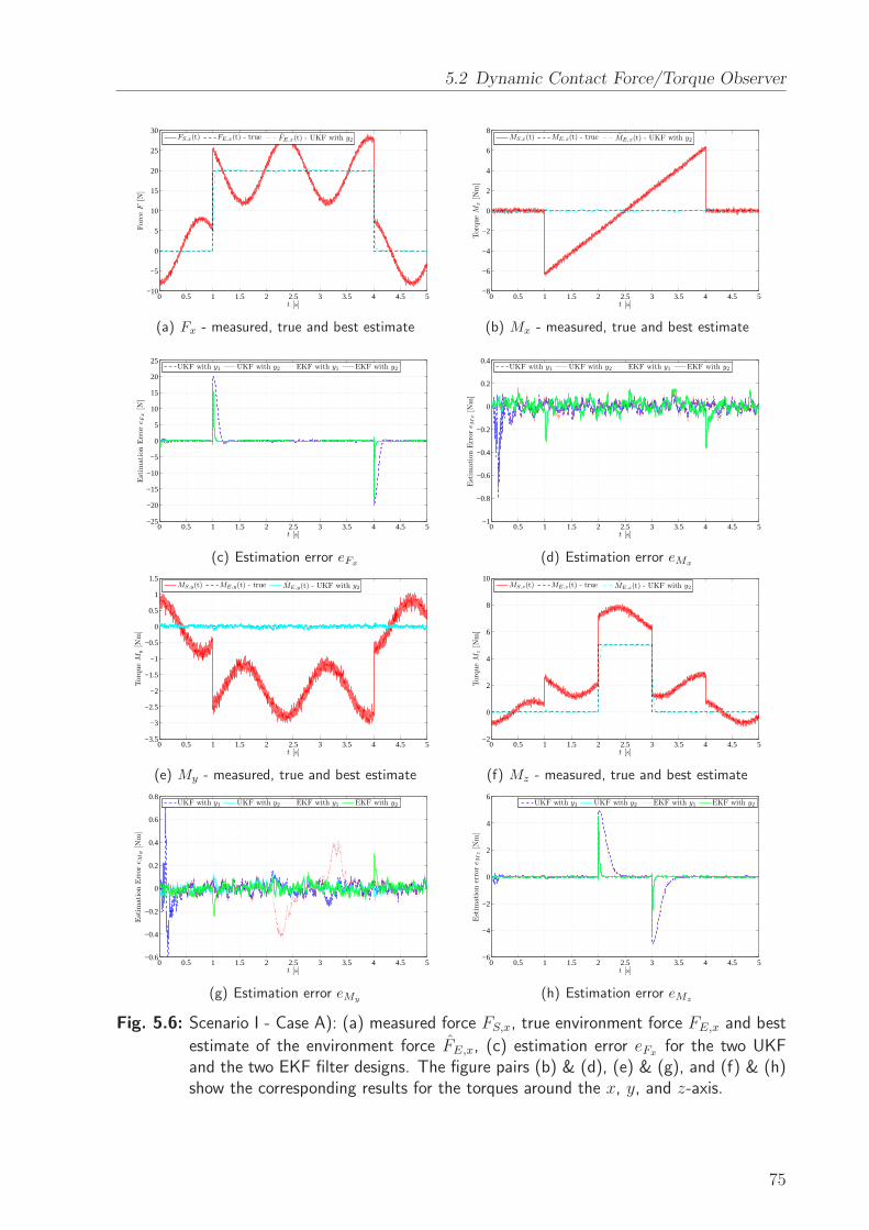
5.2 Dynamic Contact Force/Torque Observer
0 0.5 1 1.5 2 2.5 3 3.5 4 4.5 5−10
−5
0
5
10
15
20
25
30
t [s]
For
ceF
[N]
FS,x(t) FE,x(t) - true FE,x(t) - UKF with y2
(a) Fx - measured, true and best estimate
0 0.5 1 1.5 2 2.5 3 3.5 4 4.5 5−8
−6
−4
−2
0
2
4
6
8
t [s]
Tor
que
Mx
[Nm
]
MS,x(t) ME,x(t) - true ME,x(t) - UKF with y2
(b) Mx - measured, true and best estimate
0 0.5 1 1.5 2 2.5 3 3.5 4 4.5 5−25
−20
−15
−10
−5
0
5
10
15
20
25
t [s]
Est
imat
ion
Err
oreF
x[N
]
UKF with y1 UKF with y2 EKF with y1 EKF with y2
(c) Estimation error eFx
0 0.5 1 1.5 2 2.5 3 3.5 4 4.5 5−1
−0.8
−0.6
−0.4
−0.2
0
0.2
0.4
t [s]
Est
imat
ion
Err
oreM
x[N
m]
UKF with y1 UKF with y2 EKF with y1 EKF with y2
(d) Estimation error eMx
0 0.5 1 1.5 2 2.5 3 3.5 4 4.5 5−3.5
−3
−2.5
−2
−1.5
−1
−0.5
0
0.5
1
1.5
t [s]
Tor
que
My
[Nm
]
MS,y(t) ME,y(t) - true ME,y(t) - UKF with y2
(e) My - measured, true and best estimate
0 0.5 1 1.5 2 2.5 3 3.5 4 4.5 5−2
0
2
4
6
8
10
t [s]
Tor
que
Mz
[Nm
]
MS,z(t) ME,z(t) - true ME,z(t) - UKF with y2
(f) Mz - measured, true and best estimate
0 0.5 1 1.5 2 2.5 3 3.5 4 4.5 5−0.6
−0.4
−0.2
0
0.2
0.4
0.6
0.8
t [s]
Est
imat
ion
Err
oreM
y[N
m]
UKF with y1 UKF with y2 EKF with y1 EKF with y2
(g) Estimation error eMy
0 0.5 1 1.5 2 2.5 3 3.5 4 4.5 5−6
−4
−2
0
2
4
6
t [s]
Est
imat
ion
erro
reM
z[N
m]
UKF with y1 UKF with y2 EKF with y1 EKF with y2
(h) Estimation error eMz
Fig. 5.6: Scenario I - Case A): (a) measured force FS,x, true environment force FE,x and best
estimate of the environment force FE,x, (c) estimation error eFxfor the two UKF
and the two EKF filter designs. The figure pairs (b) & (d), (e) & (g), and (f) & (h)show the corresponding results for the torques around the x, y, and z-axis.
75

5Percep
tionan
dInteraction
Con
trolfor
Dynam
icMan
ipulation
0
10
20
30
40
50
60
70
80
90
100E
rror
mea
sure
impro
vem
ent
[%]
eF,Σ eF,c eF,d eM,Σ eM,c eM,d
EKF with y1 EKF with y2 UKF with y1 UKF with y2
(a) Case A
0
10
20
30
40
50
60
70
80
90
100
Err
orm
easu
reim
pro
vem
ent
[%]
eF,Σ eF,c eF,d eM,Σ eM,c eM,d
EKF with y1 EKF with y2 UKF with y1 UKF with y2
(b) Case B
0
10
20
30
40
50
60
70
80
90
100
Err
orm
easu
reim
pro
vem
ent
[%]
eF,Σ eF,c eF,d eM,Σ eM,c eM,d
EKF with y1 EKF with y2 UKF with y1 UKF with y2
(c) Case C
Fig. 5.7: Error measures: Improvements of the four filter designs compared to the measurements F S, MS.
Case A Case B Case C
eF,Σ eF,c eF,d eM,Σ eM,c eM,d eF,Σ eF,c eF,d eM,Σ eM,c eM,d eF,Σ eF,c eF,d eM,Σ eM,c eM,d
meas. FS ,MS 28.37 17.37 11.00 23.57 12.60 10.97 28.37 17.37 11.00 23.57 12.60 10.97 28.37 17.37 11.00 23.57 12.60 10.97
EKF with y1 5.02 0.86 4.16 2.27 0.32 1.94 11.33 2.31 9.03 4.55 1.10 3.46 10.01 4.83 5.18 4.08 1.81 2.27
UKF with y1 4.95 0.87 4.08 2.28 0.38 1.90 10.41 1.48 8.93 3.72 0.56 3.17 10.22 5.11 5.11 3.33 1.30 2.03
EKF with y2 1.81 0.73 1.08 0.65 0.25 0.40 10.20 3.09 7.11 2.59 0.42 2.17 2.67 1.57 1.10 1.30 0.77 0.54
UKF with y2 1.72 0.68 1.04 0.62 0.25 0.37 9.68 2.79 6.89 2.47 0.37 2.10 2.66 1.56 1.09 1.29 0.76 0.53
Tab. 5.1: Scenario I: Error measures eM,Σ, eF,c, eF,d, eM,Σ, eM,c, and eM,d for the different filter designs and cases A) - C). In each column,the filter with the best performance is highlighted.
76
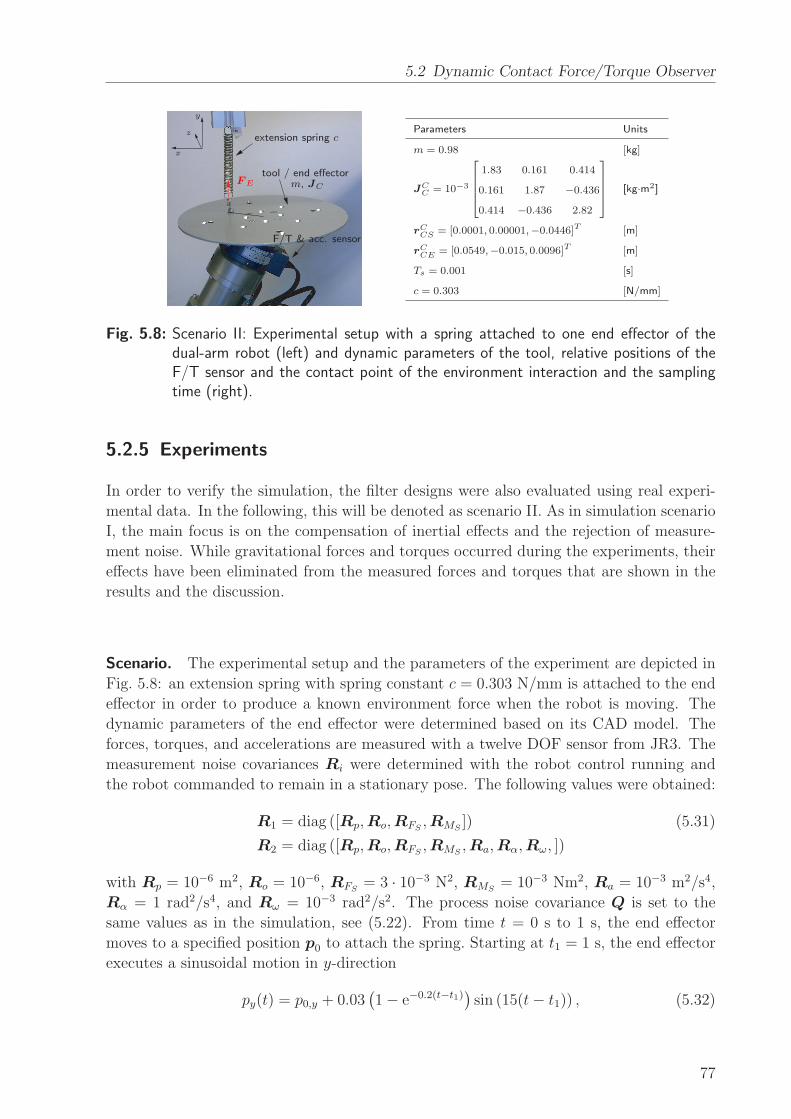
5.2 Dynamic Contact Force/Torque Observer
extension spring c
tool / end effectorm, JC
x
y
z
FE
F/T & acc. sensor
Parameters Units
m = 0.98 [kg]
JCC = 10−3
1.83 0.161 0.414
0.161 1.87 −0.436
0.414 −0.436 2.82
[kg·m2]
rCCS = [0.0001, 0.00001,−0.0446]T [m]
rCCE = [0.0549,−0.015, 0.0096]T [m]
Ts = 0.001 [s]
c = 0.303 [N/mm]
Fig. 5.8: Scenario II: Experimental setup with a spring attached to one end effector of thedual-arm robot (left) and dynamic parameters of the tool, relative positions of theF/T sensor and the contact point of the environment interaction and the samplingtime (right).
5.2.5 Experiments
In order to verify the simulation, the filter designs were also evaluated using real experi-
mental data. In the following, this will be denoted as scenario II. As in simulation scenario
I, the main focus is on the compensation of inertial effects and the rejection of measure-
ment noise. While gravitational forces and torques occurred during the experiments, their
effects have been eliminated from the measured forces and torques that are shown in the
results and the discussion.
Scenario. The experimental setup and the parameters of the experiment are depicted in
Fig. 5.8: an extension spring with spring constant c = 0.303 N/mm is attached to the end
effector in order to produce a known environment force when the robot is moving. The
dynamic parameters of the end effector were determined based on its CAD model. The
forces, torques, and accelerations are measured with a twelve DOF sensor from JR3. The
measurement noise covariances Ri were determined with the robot control running and
the robot commanded to remain in a stationary pose. The following values were obtained:
R1 = diag ([Rp,Ro,RFS,RMS
]) (5.31)
R2 = diag ([Rp,Ro,RFS,RMS
,Ra,Rα,Rω, ])
with Rp = 10−6 m2, Ro = 10−6, RFS= 3 · 10−3 N2, RMS
= 10−3 Nm2, Ra = 10−3 m2/s4,
Rα = 1 rad2/s4, and Rω = 10−3 rad2/s2. The process noise covariance Q is set to the
same values as in the simulation, see (5.22). From time t = 0 s to 1 s, the end effector
moves to a specified position p0 to attach the spring. Starting at t1 = 1 s, the end effector
executes a sinusoidal motion in y-direction
py(t) = p0,y + 0.03(
1− e−0.2(t−t1))
sin (15(t− t1)) , (5.32)
77
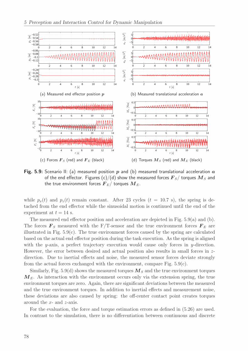
5 Perception and Interaction Control for Dynamic Manipulation
0 2 4 6 8 10 12 14−0.58−0.56−0.54−0.52
px
[m]
0 2 4 6 8 10 12 14
−0.12−0.1
−0.08−0.06
py
[m]
0 2 4 6 8 10 12 14
−0.3−0.28−0.26−0.24
t [s]
pz
[m]
(a) Measured end effector position p
0 2 4 6 8 10 12 14
−505
ax
[m/s
2]
0 2 4 6 8 10 12 14
−505
ay
[m/s
2]
0 2 4 6 8 10 12 14
−505
t [s]
az
[m/s
2]
(b) Measured translational acceleration a
0 2 4 6 8 10 12 14−10
0
10
Fx
[N]
0 2 4 6 8 10 12 14−10
0
10
Fy
[N]
0 2 4 6 8 10 12 14−2
0
2
t [s]
Fz
[N]
(c) Forces F S (red) and FE (black)
0 2 4 6 8 10 12 14−0.5
0
0.5
Mx
[Nm
]
0 2 4 6 8 10 12 14−0.5
0
0.5
My
[Nm
]
0 2 4 6 8 10 12 14−0.5
0
0.5
t [s]
Mz
[Nm
]
(d) Torques MS (red) and ME (black)
Fig. 5.9: Scenario II: (a) measured position p and (b) measured translational acceleration a
of the end effector. Figures (c)/(d) show the measured forces F S/ torques MS andthe true environment forces F E/ torques ME.
while px(t) and pz(t) remain constant. After 23 cycles (t = 10.7 s), the spring is de-
tached from the end effector while the sinusoidal motion is continued until the end of the
experiment at t = 14 s.
The measured end effector position and acceleration are depicted in Fig. 5.9(a) and (b).
The forces F S measured with the F/T-sensor and the true environment forces F E are
illustrated in Fig. 5.9(c). The true environment forces caused by the spring are calculated
based on the actual end effector position during the task execution. As the spring is aligned
with the y-axis, a perfect trajectory execution would cause only forces in y-direction.
However, the error between desired and actual position also results in small forces in z-
direction. Due to inertial effects and noise, the measured sensor forces deviate strongly
from the actual forces exchanged with the environment, compare Fig. 5.9(c).
Similarly, Fig. 5.9(d) shows the measured torquesMS and the true environment torques
ME. As interaction with the environment occurs only via the extension spring, the true
environment torques are zero. Again, there are significant deviations between the measured
and the true environment torques. In addition to inertial effects and measurement noise,
these deviations are also caused by spring: the off-center contact point creates torques
around the x- and z-axis.
For the evaluation, the force and torque estimation errors as defined in (5.26) are used.
In contrast to the simulation, there is no differentiation between continuous and discrete
78

5.2 Dynamic Contact Force/Torque Observer
phases. Hence, only the combined error measures eF,Σ and eM,Σ are utilized for the evalu-
ation of the performance, compare (5.30).
Results. The measured sensor force, the true environment force, and the estimated en-
vironment force (UKF with y2) in y-direction are depicted in Fig. 5.10(a). The force
estimation errors for the four different filter designs are illustrated in Fig. 5.10(b). For the
two observers based on measurement vector y1, the estimation error shows very similar
behavior: during contact with the environment, the estimates lag behind the actual forces
leading to errors of up to 7 N. The estimation errors of the y2-based designs are also almost
identical. However, the maximum estimation error for these designs is only 1.8 N. From
Fig. 5.10(a), it is evident that measured sensor forces can not be directly used in a force
control scheme: in both phases, there is a significant deviation between the measurements
and the actual environment forces. During the contact phase (from 1 s to 10.8 s), the
environment/spring force F E partially compensates the inertial forces F I . During the free
space motion (10.8 s to 14 s), the measured forces reflect the inertial forces caused by the
sinusoidal motion with increasing amplitude.
The measured sensor torques, the true environment torques, and the estimated envi-
ronment torques (UKF with y2) around the x- and z-axis are depicted in Fig. 5.12(a)
and (c). The corresponding estimation errors for the four filters are shown in Fig. 5.12(b)
and (d). As for the forces, the estimation errors for UKF and EKF with the same measure-
ment vector are very similar. Furthermore, the maximum errors of the y2-based designs
(0.04 Nm) are considerably lower than those of the filters with y1 (0.1 Nm). In analogy to
the forces, the deviations between measured torques MS and actual environment torques
ME depicted in Fig. 5.12(a) and (c) illustrate the importance of the observer for a reliable
force control performance.
Discussion. The quantitative results are summarized in Fig. 5.11 using the two error
measures eF,Σ and eM,Σ. Again, the first row of the table shows the values of the error
measures when the measured forces F S and torques MS are assumed to be identical with
the environment forces and torques. This can be considered as the worst case scenario.
When using an observer design based on y1 (pose and F/T measurements), the combined
error measures eF,Σ (eM,Σ) can be reduced by appr. 57% (80%) compared to the worst
case scenario. Here, EKF and UKF design are performing almost equally well. By adding
an acceleration sensor and using measurements y2 fused from the three sensor types, the
performance can be further improved: The combined error measure eF,Σ is reduced by
74.7 % for the EKF and by 74.6 % for the UKF (compared to the filter with y1). The
same holds for the combined error measure eM,Σ when a filter design with y2 instead of y1
is used: The measure is reduced by 61.3% for the EKF and by 60.5% for the UKF.
Overall, the experimental results are in accordance with those of the simulation: First,
EKF and UKF based observer designs perform almost equally well. Second, the designs
with the extended measurement vector y2 show a significant performance improvement
compared to designs based on y1. The observers with y1, in turn, still show significant
improvements compared to the measured values.
79
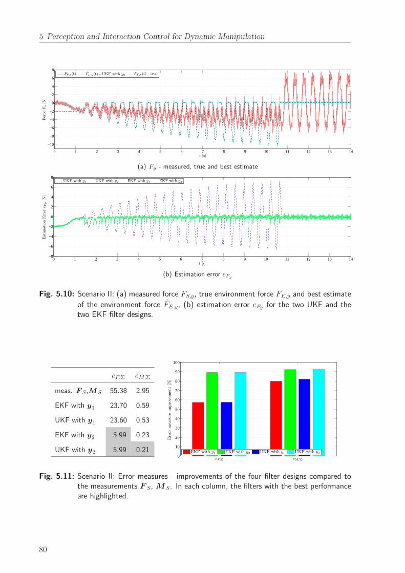
5 Perception and Interaction Control for Dynamic Manipulation
0 1 2 3 4 5 6 7 8 9 10 11 12 13 14
−10
−8
−6
−4
−2
0
2
4
6
8
t [s]
For
ceF
y[N
]
FS,y(t) FE,y (t) - UKF with y2FE,y(t) - true
(a) Fy - measured, true and best estimate
0 1 2 3 4 5 6 7 8 9 10 11 12 13 14−8
−6
−4
−2
0
2
4
6
8
t [s]
Est
imat
ion
Err
ore F
y[N
]
UKF with y1 UKF with y2 EKF with y1 EKF with y2
(b) Estimation error eFy
Fig. 5.10: Scenario II: (a) measured force FS,y, true environment force FE,y and best estimate
of the environment force FE,y, (b) estimation error eFyfor the two UKF and the
two EKF filter designs.
eF,Σ eM,Σ
meas. F S ,MS 55.38 2.95
EKF with y1 23.70 0.59
UKF with y1 23.60 0.53
EKF with y2 5.99 0.23
UKF with y2 5.99 0.210
10
20
30
40
50
60
70
80
90
100
Err
orm
easu
reim
pro
vem
ent
[%]
eF,Σ eM,Σ
EKF with y1 EKF with y2 UKF with y1 UKF with y2
Fig. 5.11: Scenario II: Error measures - improvements of the four filter designs compared tothe measurements F S, MS. In each column, the filters with the best performanceare highlighted.
80

5.2 Dynamic Contact Force/Torque Observer
0 1 2 3 4 5 6 7 8 9 10 11 12 13 14−0.1
0
0.1
0.2
0.3
0.4
t [s]
Tor
que
Mx
[Nm
]
MS,x(t) ME,x(t) - UKF with y2ME,x(t) - true
(a) Mx - measured, true and best estimate
0 1 2 3 4 5 6 7 8 9 10 11 12 13 14−0.06
−0.04
−0.02
0
0.02
0.04
0.06
t [s]
Est
imat
ion
Err
ore M
x[N
m]
UKF with y1 UKF with y2 EKF with y1 EKF with y2
(b) Estimation error eMx
0 1 2 3 4 5 6 7 8 9 10 11 12 13 14−0.8
−0.6
−0.4
−0.2
0
0.2
0.4
0.6
t [s]
Tor
que
Mz
[Nm
]
MS,z(t) ME,z (t) - UKF with y2ME,z(t) - true
(c) Mz - measured, true and best estimate
0 1 2 3 4 5 6 7 8 9 10 11 12 13 14−0.1
−0.05
0
0.05
0.1
0.15
t [s]
Est
imat
ion
erro
re M
z[N
m]
UKF with y1 UKF with y2 EKF with y1 EKF with y2
(d) Estimation error eMz
Fig. 5.12: Scenario II: (a) measured forceMS,x, true environment forceME,x and best estimate
of the environment force ME,x, (b) estimation error eMxfor the two UKF and the
two EKF filter designs. The figure pair (c) & (d) shows the corresponding resultsfor the torque around the z-axis.
81
5 Perception and Interaction Control for Dynamic Manipulation
5.3 Motion and Interaction Control
The following section summarizes the robot control strategies that have been utilized in this
thesis. Here, two different tasks have to be considered: first, the control of the robot during
free space motions. Second, the interaction control of the robot when the manipulator is in
contact with the environment. The former is realized with the inverse dynamics approach,
the latter with a parallel force/position control scheme. In both cases, the task space
formalism is used.
Commonly, interaction control schemes assume that the weight and the inertia of the
tool are negligible [125]. Since this assumption does not hold for dynamic manipulation
tasks, it is necessary to modify the interaction control scheme with the dynamic contact
force/torque observer that has been presented in the previous section.
A detailed discussion on interaction control schemes can be found in [94]. For the dual-
arm robot used in this work, impedance control schemes were evaluated by Stanczyk [132].
5.3.1 Task Space Motion Control
In general, the pose of the end effector is defined by
xM =[
pTM oTM]T, (5.33)
where pM ∈ R3 denotes the position and oM the orientation of the end effector. In oper-
ational space control, the orientation is described with three Euler angles. These are the
minimal set of variables to represent orientation, resulting in xM ∈ R6. However, such an
approach has two drawbacks: first, Euler angles have representation singularities. Second,
they are inconsistent with the task geometry, see Natale for a detailed discussion [94].
To overcome these drawbacks, task space control schemes have been proposed, see e.g.
Caccavale et al. [26]. Here, the orientation is represented using a non-minimal set of
variables based on an angle-axis description. The most common angle-axis notation are
unit quaternions, which are also used in this work. Consequently, the pose of the end
effector is given by xM =[
pTM oTe]T
∈ R7 with oM = η, ǫ. Details on the quaternion
notation are given in App. A.3. When referring to the end effector pose xM , the following
secondary subscripts are used: d (desired), a (actual), c (compliant), r (reference).
The dynamic model of a robot manipulator is given by
B(q)q +C(q, q)q + f(q, q) + g(q) = τ − JT (q)T E ∈ Rn (5.34)
where B(q) is the inertia matrix, C(q, q)q the coriolis and centrifugal torques, f(q, q) /
g(q) the frictional / gravitational torques, τ the joint driving torques, J(q) the manipu-
lator jacobian and T E =[
F TE MT
E
]Tthe vector of environment forces/torques [126].
A block scheme of the motion control is shown in Fig. 5.13 as the gray part of the
interaction control. It consists of three main modules: forward kinematics, pose control,
and inverse dynamics.
82
5.3 Motion and Interaction Control
Pose control. Given a (desired) reference trajectory (xM,r, xM,r, and xM,r) and the ac-
tual robot pose and velocity (xM,a, xM,a), the module determines the resolved acceleration
aM in task space variables as
aM =
[
aM,p
aM,o
]
=
[
pM,r +KDp∆pM,ra +KPp∆pM,ra
ωM,r +KDo∆ωM,ra +KPoRMǫM,ra
]
(5.35)
where ∆pM,ra and ∆ωM,ra are the velocity tracking errors, ∆pM,ra and ǫM,ra the pose
tracking errors, and KDp, KPp, KDo, and KPo are matrix gains as detailed in [94].
Inverse dynamics. The inverse dynamics module applies the feedback linearization tech-
nique to the robotic system in order to obtain a linear and decoupled system. To this
end, the module calculates the joint torques that match the resolved acceleration. This is
realized in two steps: first, the joint accelerations q that correspond to the resolved end
effector acceleration have to be determined,
q = J−1(q)(
aM − J(q, q))
. (5.36)
In the second step, the equivalent joint torques are calculated based on the dynamic model
given in (5.34).
Friction compensation. As part of the feedback linearization performed in the inverse
dynamics module, a model for the joint friction is needed. Commonly, a viscous friction
model is utilized because of its simplicity [94, 126]. While this is easy to implement, it
captures only a part of the friction phenomena discussed in Sec. 2.5. Clearly, the accuracy
of the friction compensator is highly dependent on the validity of the used model. For
dynamic manipulation tasks, a large range of joint velocities occurs. Hence, it is necessary
to adopt a friction model that is describing all the relevant effects. In this work, a static
friction model is utilized that considers Coulomb, viscous, and static friction and also
includes the Stribeck effect.
5.3.2 Interaction Control
Sec. 5.1 presented a brief overview on interaction control strategies. Comparing the existing
concepts, the parallel approach developed by Chiaverini and Sciavicco is the best choice
for the dynamic manipulation tasks considered in this work. This is due to two reasons:
first, the method allows to specify the desired interaction forces/torques directly. Second,
in contrast to hybrid force/position control, the controller structure does not need to be
changed during different stages of the task execution [28].
The parallel approach, like all interaction control schemes, utilizes the measured sensor
forces F S and torques MS either directly or after applying a low-pass filter [125]. This is
reasonable, as in most tasks, the weight and the inertia of the tool are negligible. However,
this assumption does not hold for dynamic robot motions where interaction forces occur
during phases with significant acceleration of the end effector. Hence, it is necessary to
83

5 Perception and Interaction Control for Dynamic Manipulation
Robot &
Environment
Parallel
Composition
Force
Control
Dynamic F/T Observer
Robot
Action
Planning
Pose
Control
Inverse
Dynamics
Forward
Kinematics
replacements
xM,d
xM,d
xM,d
xM,r
xM,r
xM,r
xM,c xM,c xM,c
τaM
FE , MEFE , ME
FE,d
ME,d
q
xM,a
xM,a
xM,a
Fig. 5.13: Block diagram of the motion control (in gray) and the overall interaction controlscheme based on parallel composition.
extend the force control scheme with one of the dynamic contact force/torque observer
designs discussed in Sec. 5.2.
Fig. 5.13 shows the parallel approach for direct force control used in this work. The
task space motion control is extended by adding two modules: force control and parallel
composition. In the following, the two modules are briefly summarized. For a detailed
discussion, see [28, 94]. In contrast to the original scheme, the control does not use the
sensor forces/torques F S/MS but the observed quantities F E/ME.
Force control. The module determines a compliant trajectory xM,c, xM,c, and xM,c based
on the differential equations
KAF pM,c +KV F pM,c = F E,d − F E
KAM ωcM,c +KVMωc
M,c = M cE,d −M c
E, (5.37)
where KAF , KV F , KAM , and KVM are matrix gains and the resulting compliant pose
xM,c incorporates an integral control action over the force/torque error [94].
Parallel composition. When using unit quaternion notation, the parallel composition of
the desired and the compliant trajectory is defined as
pM,r = pM,c + pM,d pM,r = pM,c + pM,d pM,r = pM,c + pM,d (5.38)
oM,r = oM,c ∗ oM,dc ωcM,r = ωc
M,c + ωcM,dc ωc
M,r = ωcM,c + ωc
M,dc. (5.39)
For conflicting situations, the integral control action for the compliant pose ensures domi-
nance of the force control, see (5.37).
84
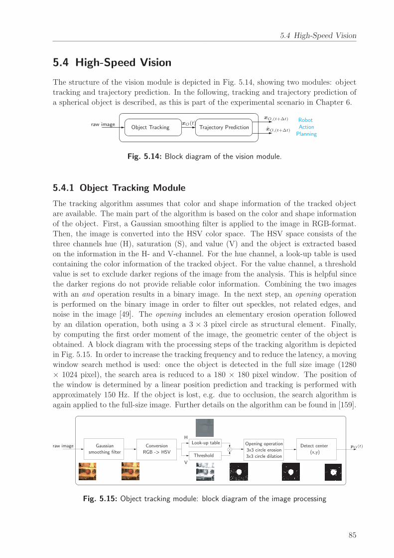
5.4 High-Speed Vision
5.4 High-Speed Vision
The structure of the vision module is depicted in Fig. 5.14, showing two modules: object
tracking and trajectory prediction. In the following, tracking and trajectory prediction of
a spherical object is described, as this is part of the experimental scenario in Chapter 6.
Robot Action
PlanningObject Tracking Trajectory Prediction
raw image
xO,(t+∆t)
xO,(t+∆t)
xO(t)
Fig. 5.14: Block diagram of the vision module.
5.4.1 Object Tracking Module
The tracking algorithm assumes that color and shape information of the tracked object
are available. The main part of the algorithm is based on the color and shape information
of the object. First, a Gaussian smoothing filter is applied to the image in RGB-format.
Then, the image is converted into the HSV color space. The HSV space consists of the
three channels hue (H), saturation (S), and value (V) and the object is extracted based
on the information in the H- and V-channel. For the hue channel, a look-up table is used
containing the color information of the tracked object. For the value channel, a threshold
value is set to exclude darker regions of the image from the analysis. This is helpful since
the darker regions do not provide reliable color information. Combining the two images
with an and operation results in a binary image. In the next step, an opening operation
is performed on the binary image in order to filter out speckles, not related edges, and
noise in the image [49]. The opening includes an elementary erosion operation followed
by an dilation operation, both using a 3 × 3 pixel circle as structural element. Finally,
by computing the first order moment of the image, the geometric center of the object is
obtained. A block diagram with the processing steps of the tracking algorithm is depicted
in Fig. 5.15. In order to increase the tracking frequency and to reduce the latency, a moving
window search method is used: once the object is detected in the full size image (1280
× 1024 pixel), the search area is reduced to a 180 × 180 pixel window. The position of
the window is determined by a linear position prediction and tracking is performed with
approximately 150 Hz. If the object is lost, e.g. due to occlusion, the search algorithm is
again applied to the full-size image. Further details on the algorithm can be found in [159].
Gaussian
smoothing filter
Conversion
RGB -> HSV
raw image Opening operation
3x3 circle erosion
3x3 circle dilation
Detect center
(x,y)
Look-up table
Threshold
H
V
pO(t)
Fig. 5.15: Object tracking module: block diagram of the image processing
85
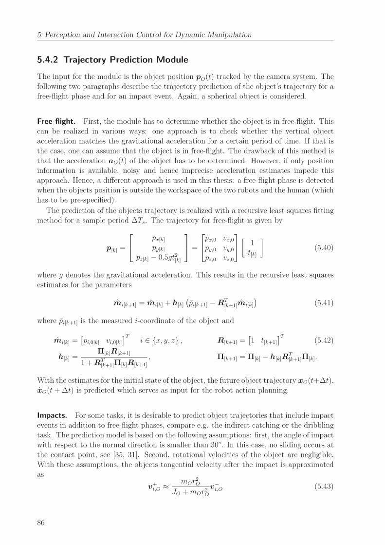
5 Perception and Interaction Control for Dynamic Manipulation
5.4.2 Trajectory Prediction Module
The input for the module is the object position pO(t) tracked by the camera system. The
following two paragraphs describe the trajectory prediction of the object’s trajectory for a
free-flight phase and for an impact event. Again, a spherical object is considered.
Free-flight. First, the module has to determine whether the object is in free-flight. This
can be realized in various ways: one approach is to check whether the vertical object
acceleration matches the gravitational acceleration for a certain period of time. If that is
the case, one can assume that the object is in free-flight. The drawback of this method is
that the acceleration aO(t) of the object has to be determined. However, if only position
information is available, noisy and hence imprecise acceleration estimates impede this
approach. Hence, a different approach is used in this thesis: a free-flight phase is detected
when the objects position is outside the workspace of the two robots and the human (which
has to be pre-specified).
The prediction of the objects trajectory is realized with a recursive least squares fitting
method for a sample period ∆Ts. The trajectory for free-flight is given by
p[k] =
px[k]py[k]
pz[k] − 0.5gt2[k]
=
px,0 vx,0py,0 vy,0pz,0 vz,0
[
1
t[k]
]
(5.40)
where g denotes the gravitational acceleration. This results in the recursive least squares
estimates for the parameters
mi[k+1] = mi[k] + h[k]
(
pi[k+1] −RT[k+1]mi[k]
)
(5.41)
where pi[k+1] is the measured i-coordinate of the object and
mi[k] =[
pi,0[k] vi,0[k]]T
i ∈ x, y, z , R[k+1] =[
1 t[k+1]
]T(5.42)
h[k] =Π[k]R[k+1]
1 +RT[k+1]Π[k]R[k+1]
, Π[k+1] = Π[k] − h[k]RT[k+1]Π[k].
With the estimates for the initial state of the object, the future object trajectory xO(t+∆t),
xO(t+∆t) is predicted which serves as input for the robot action planning.
Impacts. For some tasks, it is desirable to predict object trajectories that include impact
events in addition to free-flight phases, compare e.g. the indirect catching or the dribbling
task. The prediction model is based on the following assumptions: first, the angle of impact
with respect to the normal direction is smaller than 30. In this case, no sliding occurs at
the contact point, see [35, 31]. Second, rotational velocities of the object are negligible.
With these assumptions, the objects tangential velocity after the impact is approximated
as
v+t,O ≈
mOr2O
JO +mOr2Ov−t,O (5.43)
86
5.5 Summary
where JO denotes the moment of inertia of the ball. Inserting the expression for a spherical
shell, JO = 23mOr
2O, in (5.43) leads to a proportionality constant cr,t = 0.6 for the horizontal
velocities before and after the impact, compare Sec. 2.6. The translational object velocity
after the ground impact is hence defined as
v+O =
[
cr,t cr,t −cr]T
v−O (5.44)
where cr is the coefficient of restitution for the ground impact.
The models for the free flight phase and the impact event provide the possibility to
predict the future object trajectory which is then used for the robot action planning.
5.5 Summary
This chapter discussed environment perception and interaction control for dynamic object
manipulation. Clearly, precise motion/interaction control and accurate sensor feedback are
essential for the execution of such tasks on real robotic hardware. However, the dynamic
nature of the tasks poses particular challenges that need to be considered.
In Section 5.2, a sensor fusion approach for improved interaction control and estima-
tion of environment forces and torques was presented. The continuous- and discrete-time
system model was derived using quaternion notation for the description of the tool ori-
entation. Based on the system model, the design of six DOF force/torque observers was
discussed. Here, designs based on the EKF and on the UKF were presented. For both de-
signs, two different measurement vectors have been considered: the first one uses pose and
F/T measurements while the second one also uses acceleration and (rotational) velocity
measurements. The four filter designs were first evaluated in a six DOF simulation sce-
nario. Particular interest was paid to the robustness of the filter designs towards changing
environment conditions. To this end, the simulation was performed in three different con-
ditions: a perfectly known, an overestimated, and an underestimated measurement noise.
Six error measures were introduced to evaluate the performance for force and torque es-
timation during continuous and discrete phases. Despite the decline in performance, the
variation of the measurement noise showed that the filters can significantly improve the
contact force/torque estimation even for inaccurate estimates of the measurement noise
levels. For the observer designs with extended measurement vector, the underestimation
of the measurement noise was less critical than the overestimation. For the designs with
pose and F/T measurements, the effects of over- and underestimation were comparable.
In addition to the simulation, a six DOF experiment was conducted to verify the results.
For both, simulation and experiment, the UKF with the extended measurement vector
performed best. Although it showed in most of cases only small improvements compared
to the EKF with extended measurements, it offers the additional benefit that the calcula-
tion of process and measurement jacobians is not needed which makes the UKF easier to
implement.
In Section 5.3, the motion and interaction control schemes for the robotic manipulators
were discussed. The motion control is realized in task space with the well-established
inverse dynamics approach. For the interaction control, a direct force control scheme based
87

5 Perception and Interaction Control for Dynamic Manipulation
on parallel composition is used. To meet the demands of dynamic object manipulation,
the scheme was augmented with the dynamic force/torque observer which provides the
estimated environment forces and torques for the interaction control.
In Section 5.4, a method for object tracking with high frame rates (appr. 150 Hz) was
detailed. In addition to the tracking algorithm, the section discussed the trajectory pre-
diction for spherical objects. The prediction is based on the models discussed in Chapter 2
and was presented for free-flight phases and impact events as these are of particular inter-
est for the case studies considered in this thesis. However, the prediction can be used in a
similar way for other motion phases, such as rolling or sliding.
88
6 Experimental Evaluation
Summary Experimental results of dynamic object manipulation are presented: nonpre-
hensile catching, throwing, dribbling, and juggling tasks are performed with a six DOF
industrial robot and a 14 DOF anthropomorphic dual-arm manipulator. The results of
the previous chapters with respect to modeling, environment perception, planning, and
control design are integrated in a robotic basketball demonstration scenario. In addition,
the benefits of a compliant end effector design are demonstrated by comparing the perfor-
mance of the compliant and the rigid end effector design for the dribbling task. Finally, the
experiments provide valuable insights into practical issues that have not been considered
in the theoretical analysis.
The experimental evaluation focuses on robotic basketball as demonstration scenario.
Basketball is an excellent challenge to study dynamic and interactive manipulation: the
game incorporates intrinsically dynamic manipulation tasks such as catching, throwing,
and dribbling. The execution of these tasks requires a high degree of mobility, a de-
tailed environment perception, and a precise timing of motions. Furthermore, the scenario
demonstrates exemplarily that dexterous manipulation skills can be realized with simpli-
fied end effector designs. Equipping robots with such a dynamic dexterity is particularly
helpful for the handling of objects that are oversized for conventional grippers.
The chapter is organized as follows: Section 6.1 introduces the hardware setup used for
the experiments. Then, Section 6.2 presents results of the throwing experiments that have
been performed with the dual-arm manipulator. Next, Section 6.3 details the nonprehensile
catching experiments that have been conducted. Both, direct and indirect catching have
been realized in experiments. Section 6.4 shows experimental results for ball dribbling
and considers two different end effector designs: dribbling with a rigid end effector is
detailed in Subsection 6.4.1 and dribbling with a compliant end effector is presented in
Subsection 6.4.2. A comparison of the two dribbling tasks is presented in Subsection 6.4.3.
Finally, Section 6.5 shows results for the classic juggling tasks performed with the dual-arm
manipulator in open-loop control.
89
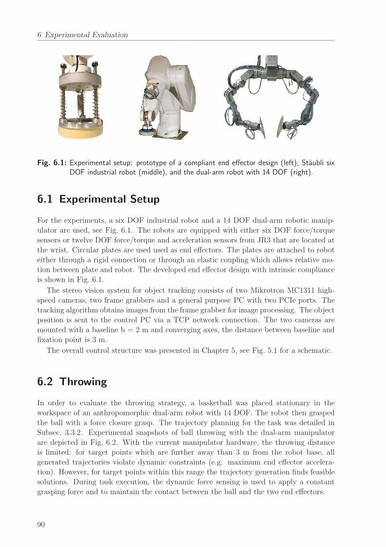
6 Experimental Evaluation
Fig. 6.1: Experimental setup: prototype of a compliant end effector design (left), Staubli sixDOF industrial robot (middle), and the dual-arm robot with 14 DOF (right).
6.1 Experimental Setup
For the experiments, a six DOF industrial robot and a 14 DOF dual-arm robotic manip-
ulator are used, see Fig. 6.1. The robots are equipped with either six DOF force/torque
sensors or twelve DOF force/torque and acceleration sensors from JR3 that are located at
the wrist. Circular plates are used used as end effectors. The plates are attached to robot
either through a rigid connection or through an elastic coupling which allows relative mo-
tion between plate and robot. The developed end effector design with intrinsic compliance
is shown in Fig. 6.1.
The stereo vision system for object tracking consists of two Mikrotron MC1311 high-
speed cameras, two frame grabbers and a general purpose PC with two PCIe ports. The
tracking algorithm obtains images from the frame grabber for image processing. The object
position is sent to the control PC via a TCP network connection. The two cameras are
mounted with a baseline b = 2 m and converging axes, the distance between baseline and
fixation point is 3 m.
The overall control structure was presented in Chapter 5, see Fig. 5.1 for a schematic.
6.2 Throwing
In order to evaluate the throwing strategy, a basketball was placed stationary in the
workspace of an anthropomorphic dual-arm robot with 14 DOF. The robot then grasped
the ball with a force closure grasp. The trajectory planning for the task was detailed in
Subsec. 3.3.2. Experimental snapshots of ball throwing with the dual-arm manipulator
are depicted in Fig. 6.2. With the current manipulator hardware, the throwing distance
is limited: for target points which are further away than 3 m from the robot base, all
generated trajectories violate dynamic constraints (e.g. maximum end effector accelera-
tion). However, for target points within this range the trajectory generation finds feasible
solutions. During task execution, the dynamic force sensing is used to apply a constant
grasping force and to maintain the contact between the ball and the two end effectors.
90

6.3 Nonprehensile Catching
Fig. 6.2: Throwing - experimental snapshots: motion sequence of the dual-arm manipulatorfrom 0 s to 1 s.
6.3 Nonprehensile Catching
The catching task was performed with the six DOF industrial robot. It is initiated when
the human operator throws a basketball into the workspace of the robot. In the following,
experimental results for the ball trajectory prediction and the two nonprehensile catching
methods are presented.
Trajectory prediction. Once the ball is detected by the camera system, it is tracked
with appr. 150 Hz and the trajectory is predicted based on the recursive least squares
algorithm presented in Subsec. 5.4.2. If a free-flight phase is detected for 100 ms, the
prediction is used to create the end effector trajectory for direct or indirect catching which
took additional 20 ms. The results of the ball trajectory prediction for the vertical z-
and horizontal y-direction for two different sample periods ∆Ts are illustrated in Fig. 6.3.
For both, y- and z-direction, the accuracy is significantly improved when using the longer
sample period: for a prediction horizon of ∆t = 0.4 s, the deviations from the tracked
position are typically less than 0.1 m (∆Ts = 50 ms) respectively 0.02 m (∆Ts = 100 ms).
Direct catch. A snapshot sequence of a direct catch is shown in Fig. 6.4. For t < tc,
the robot adjusts its position and velocity to match the constraints at tc (snapshots 3-6),
compare Subsec. 3.3.3. Then, for t > tc, the ball is decelerated and the balancing scheme
controls the end effector orientation based on the force/torque measurements (snaps. 7-15).
Indirect catch. The ball and effector trajectories for an indirect catch are illustrated in
Fig. 6.5. For the initial contact, the end effector adjusts its orientation according to (3.18)
91
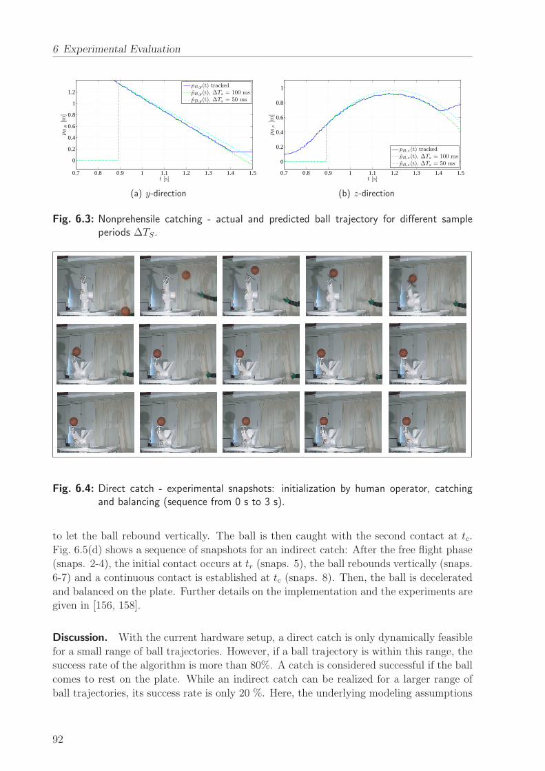
6 Experimental Evaluation
0.7 0.8 0.9 1 1.1 1.2 1.3 1.4 1.5
0
0.2
0.4
0.6
0.8
1
1.2
t [s]
pB
,y[m
]
pB,y(t) trackedpB,y(t), ∆Ts = 100 mspB,y(t), ∆Ts = 50 ms
(a) y-direction
0.7 0.8 0.9 1 1.1 1.2 1.3 1.4 1.5
0
0.2
0.4
0.6
0.8
1
t [s]
pB
,z[m
]
pB,z (t) trackedpB,z (t), ∆Ts = 100 mspB,z (t), ∆Ts = 50 ms
(b) z-direction
Fig. 6.3: Nonprehensile catching - actual and predicted ball trajectory for different sampleperiods ∆TS.
Fig. 6.4: Direct catch - experimental snapshots: initialization by human operator, catchingand balancing (sequence from 0 s to 3 s).
to let the ball rebound vertically. The ball is then caught with the second contact at tc.
Fig. 6.5(d) shows a sequence of snapshots for an indirect catch: After the free flight phase
(snaps. 2-4), the initial contact occurs at tr (snaps. 5), the ball rebounds vertically (snaps.
6-7) and a continuous contact is established at tc (snaps. 8). Then, the ball is decelerated
and balanced on the plate. Further details on the implementation and the experiments are
given in [156, 158].
Discussion. With the current hardware setup, a direct catch is only dynamically feasible
for a small range of ball trajectories. However, if a ball trajectory is within this range, the
success rate of the algorithm is more than 80%. A catch is considered successful if the ball
comes to rest on the plate. While an indirect catch can be realized for a larger range of
ball trajectories, its success rate is only 20 %. Here, the underlying modeling assumptions
92

6.4 Dribbling
0 0.25 0.5 0.75 1 1.25 1.5 1.75 2.0
0
0.5
1
1.5
t [s]
py
[m]
pB,y(t)pM,y(t)
(a) Trajectories in y-direction
0 0.25 0.5 0.75 1 1.25 1.5 1.75 2.0
0.2
0.4
0.6
0.8
1
t [s]
pz
[m]
pB,z (t)pM,z (t)
(b) Trajectories in z-direction
0 0.25 0.5 0.75 1 1.25 1.5 1.75 2.0−0.2
0
0.2
0.4
0.6
0.8
t [s]
oe
oM,1(t) oM,2(t) oM,3(t) oM,4(t)
(c) End effector orientation
(d) Initialization by human operator, initial rebound and catching (sequence from 0 s to 2 s)
Fig. 6.5: Indirect catch - ball and end effector trajectories: (a) horizontal y-direction, (b) ver-tical z-direction, (c) end effector orientation, and (d) experimental snapshots.
of the trajectory generation do not describe the impact event accurately, compare Sec. 3.3.
Clearly, the range of feasible ball trajectories is influenced by various factors and can be
improved by modifying the field of view of the camera system or the manipulator hardware.
6.4 Dribbling
For the analysis of the dribbling task in Subsec. 4.5.2 and Sec. 4.6, simplifying assumptions
were made: ball and manipulator motion were restricted to the vertical direction, impacts
were modeled as instantaneous inelastic collisions described by cr, and rotational ball
velocity was assumed to be negligible. For the hardware experiments, these modeling
errors must be considered and their effects have to be compensated.
The inputs for the robot trajectory generation are the predicted ball position in the
xy-plane pB,x(ti) and pB,y(ti), the predicted ball velocity vB(t−i ) at the impact / dribbling
height hd, and the point in time ti when hd is reached.
Trajectory prediction. The creation of a desired end effector trajectory is based on a
prediction of the ball trajectory. As depicted in Fig. 6.6(a) and 6.6(b), the two different
methods described in Subec. 5.4.2 are evaluated: a prediction before and a prediction after
the bounce on the ground. In Fig. 6.6(a), the value of the variable changes from 0 to hdwhen the next prediction of ti becomes available. Accordingly, a step down from hd to 0
occurs once the predicted time ti is reached. This means, the wider the step, the earlier
93

6 Experimental Evaluation
0.5 1 1.5 2 2.5 3 3.5
0
0.2
0.4
0.6
0.8
1
pB
,z[m
]
t [s]
pB,z(t) tracked pB,z(ti), prediction 1 pB,z(ti), prediction 2
(a) Predicted point in time ti for reaching hd
0.5 1 1.5 2 2.5 3 3.50.4
0.5
0.6
0.7
0.8
pB
,x[m
]
t [s]
pB,x(t) tracked pB,x(ti), prediction 1 pB,x(ti), prediction 2
(b) Predicted x-coordinate pB,x(ti) of the ball at hd
Fig. 6.6: Dribbling with a rigid end effector - actual and predicted ball trajectory for twoprediction horizons.
the prediction is available and for an ideal prediction, the step down will occur exactly
when the ball reaches hd. As depicted in Fig. 6.6(a), the accuracy of both approaches is
almost identical while the first approach provides the predicted value approximately 0.15 s
earlier. Fig. 6.6(b) shows that, for the prediction of the x-coordinate of the ball at the
dribbling height, the second approach is more accurate. Again, the drawback of the second
method is that it requires a faster motion execution of the robot since the time span until
the ball reaches the dribbling height hd is approximately 0.15 s smaller. In the presented
experiments, the robot trajectory is generated based on the first prediction method.
Initialization. The dribbling task can be initialized either by the human operator or the
robot. In the former case, the task is triggered when the ball is dropped into a specified
area of the robot workspace. Such an initialization is shown in Fig. 6.8. In the latter case,
the ball is initially at rest on the plate and then dropped by the robot to start the dribbling
cycle. This autonomous initialization is illustrated in Fig. 6.9.
6.4.1 Rigid End Effector
Compensation of horizontal deviations. Horizontal deviations from the desired posi-
tion are compensated by adjusting the orientation of the end effector. The orientation is
described by quaternion representation cos(φ/2), ra sin(φ/2), with axis ra in the hori-
zontal xy-plane and angle φ = 0 corresponding to an end effector plate facing the ground.
To determine the required horizontal ball velocity after the actuated impact vB,h(t+i ),
the deviations ex and ey of the ball’s x- and y-coordinate and the overall error eh in the
horizontal plane at the specified dribbling height
ex = pB,x,des(ti)− pB,x(ti) ey = pB,y,des(ti)− pB,y(ti) eh =√
e2x + e2y (6.1)
are calculated, see Fig. 6.7. Based on the deviations ex and ey, the axis of rotation
ra =1
eh
[
−ey −ex 0]T
(6.2)
is defined. The horizontal motion of the ball during one cycle is the sum of the contributions
94

6.4 Dribbling
ex
ey
x
y zpB,des(ti)
pB(ti)
ra
eh
eh
vB,h(t+i)∆tdrop vB,h(t+
gi)∆trise
Fig. 6.7: Dribbling with a rigid end effector - position error eh and axis of rotation ra.
in drop and rise phase
eh = vB,h(t+i ) (∆tdrop + cr,t∆trise) , (6.3)
which defines the required horizontal ball velocity vB,h(t+i ). With the assumption of no
sliding between the contact points during impact and neglecting rotational velocity, the
vertical and horizontal ball velocity after the impact are determined as a function of φ and
the known inputs. With small angle approximation, one obtains
vB,z(t+i ) ≈− crvB,z(t
−i ) + (1 + cr) vM,z(ti) + φ (cr,t − cr) vB,h(t
−i ) (6.4)
vB,h(t+i ) ≈ φ (cr,t + cr)
(
vB,z(t−i )− vM,z(ti)
)
+ cr,tvB,h(t−i ).
With (6.1)-(6.4), the vertical end effector velocity vM,z and the rotation angle φ are de-
termined. At time ti for which the ball is predicted to reach the dribbling height hd, the
desired position, orientation, and velocity of the end effector are
pM,des(ti) =[
pB,x(ti) pB,y(ti) hd + rB]T,
oM,des(ti) = cos(φ/2), ra sin(φ/2) ∗ oe,i, (6.5)
vM,des(ti) =[
0 0 vM,z(ti)]T.
After the impact with the ball, the end effector decelerates and returns to its initial/rest
height. During the dribbling cycle, the horizontal end effector position is adjusted to
match the tracked horizontal ball position. For further details on the implementation
and a comparison of the performance between vision-based and force/torque-based ball
tracking, see Batz et al. [151].
Dribbling cycle. The ball is held in a human’s hand and then dropped into a specified
area of the robot workspace to initialize the dribbling. With vision-based ball tracking,
dribbling for multiple cycles (> 15) is achieved. Fig. 6.8 shows a sequence of snapshots
taken during an experiment. The time duration between two consecutive snapshots is
0.16 s. The ball and end effector trajectory in vertical direction are depicted in Fig. 6.11(a).
95

6 Experimental Evaluation
Fig. 6.8: Dribbling with a rigid end effector - experimental snapshots: initialization by a humanoperator and four dribbling cycles (sequence from 0.5 s to 2.9 s).
6.4.2 Compliant End Effector
The end effector design with intrinsic compliance is depicted in Fig. 6.1. The springs
allow to store energy temporarily and release it at the end of contact, leading to possi-
ble higher accelerations. The design reduces the effective inertia to 0.3 kg during initial
contact/impact, allowing for a continuous contact phase.
Dribbling cycle. The desired initial and final states for the experimentally studied drib-
bling cycle are summarized in Table 6.1. For the experiment, a constraint for the relative
velocity between ball and manipulator at the time of initial contact is added:
xM(
tc−f)
= 0.95xB(
tc−f)
. (6.6)
For the contact phases catch and push, the control law described in Sec. 4.6 is used.
During the non-contact phase the robot trajectory is generated and updated based on the
tracked ball position and the predicted impact time. For all phases, an additional controller
is used to compensate horizontal deviations. Fig. 6.11(b) shows the actual manipulator
and ball position in vertical direction during a dribbling experiment. The ball trajectory
starts at 0.75 s when the ball is detected by the vision system. A snapshot sequence of the
initialization and the first dribbling cycle is depicted in Fig. 6.9.
The performance is mainly limited by the following aspect: in the simulation, it was
assumed that there is no energy loss in the elastic actuator. For the real actuator however,
friction forces during spring compression/elongation cause energy dissipation. This, in
turn, leads to a reduced amount of energy storage in the spring and thus a reduced energy
transfer to the ball.
96

6.4 Dribbling
Fig. 6.9: Dribbling with a compliant actuator - experimental snapshots: autonomous taskinitialization and first dribbling cycle (sequence from 0 s to 2.16 s).
initial contact switch releasexM [m] 1.605 1.65∗ 1.285xB [m] 1.32 1.38 1.00xM [m/s] 1.1438 0 −2.91∗
xB [m/s] 1.204 0 −4.26
Tab. 6.1: Initial and final states for the experimentally studied dribbling cycle. Entries markedwith ∗ are obtained through trajectory optimization.
6.4.3 Comparison
Reduced mechanical load. The use of a mechanical spring element promises to reduce
the mechanical load on the end effector. In order to evaluate this assumption, the following
experiment was conducted: a basketball impacted the end effector with a relative velocity
of 1.4 m/s. Fig. 6.10(a) shows the contact force for a rigid end effector design: during the
initial impact, the force exceeds 220 N. In contrast, Fig. 6.10(b) shows the contact force for
the compliant end effector design: here, the maximum force is significantly reduced (appr.
25 N). In addition, the compliant structure leads to a continuous contact phase after the
initial impact.
Contact phase. Fig. 6.11 depicts the vertical position of manipulator and ball during
a dribbling sequence of ten seconds for a (a) rigid and (b) compliant end effector. The
ball trajectories show significant differences: with the rigid end effector, the contact phase
reduces to an impact event. The time duration of approximately 20 ms justifies the mod-
eling assumption of an instantaneous impact, compare Sec. 4.5. This is illustrated by the
discontinuous change in the ball velocity when contact with the manipulator occurs. In
contrast, with the compliant end effector, discontinuities of the ball velocity only occur
for the ground impacts. The instantaneous impact between end effector and ball is now
replaced with a continuous contact with a catch and push phase as discussed in Subsec. 4.6.
97
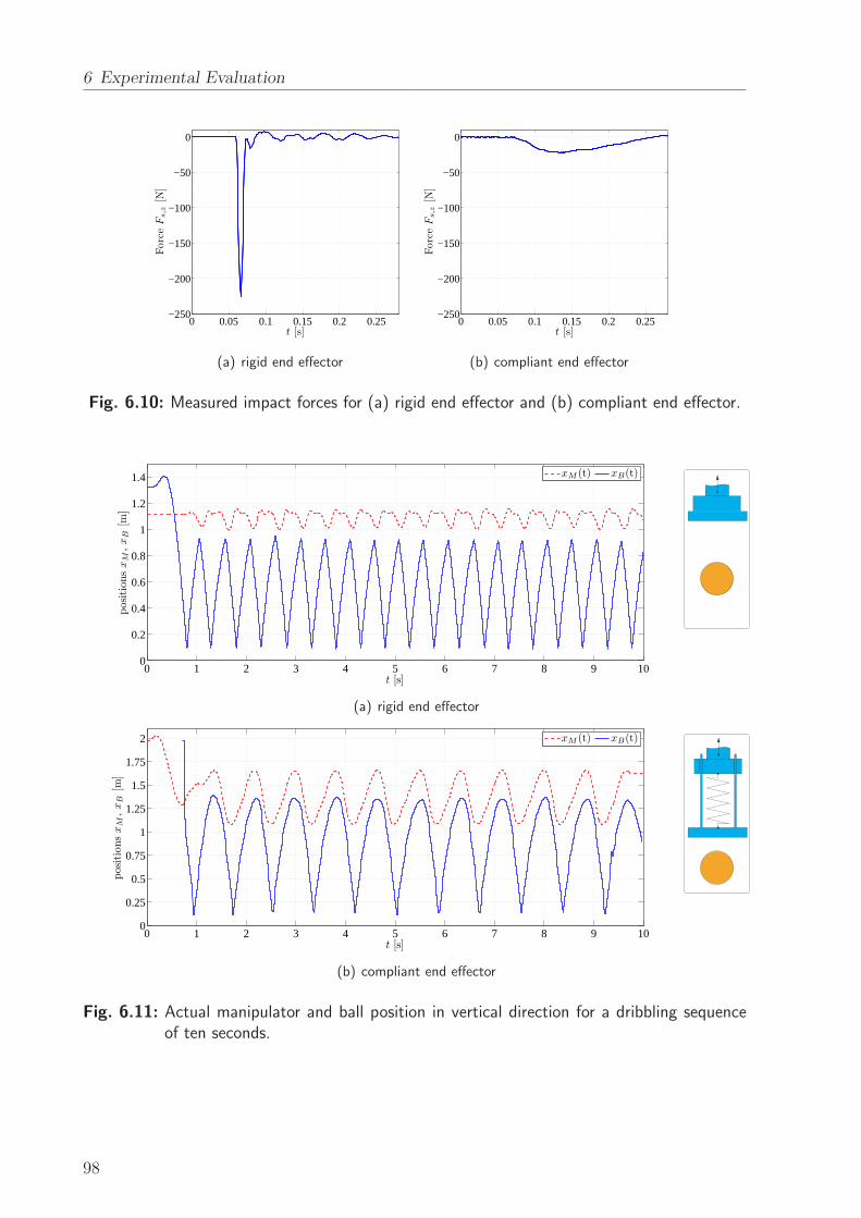
6 Experimental Evaluation
0 0.05 0.1 0.15 0.2 0.25−250
−200
−150
−100
−50
0
t [s]
Forc
eF
s,z
[N]
(a) rigid end effector
0 0.05 0.1 0.15 0.2 0.25−250
−200
−150
−100
−50
0
t [s]
Forc
eF
s,z
[N]
(b) compliant end effector
Fig. 6.10: Measured impact forces for (a) rigid end effector and (b) compliant end effector.
0 1 2 3 4 5 6 7 8 9 100
0.2
0.4
0.6
0.8
1
1.2
1.4
t [s]
positions
xM
,x
B[m
]
xM (t) xB(t)
(a) rigid end effector
0 1 2 3 4 5 6 7 8 9 100
0.25
0.5
0.75
1
1.25
1.5
1.75
2
t [s]
positions
xM
,x
B[m
]
xM (t) xB(t)
(b) compliant end effector
Fig. 6.11: Actual manipulator and ball position in vertical direction for a dribbling sequenceof ten seconds.
98

6.5 Juggling
Fig. 6.12: Juggling - experimental snapshots: motion sequence of ball and dual-armmanipulator.
6.5 Juggling
The juggling of a ping-pong ball was experimentally studied using the dual-arm manipu-
lator. The task was performed in open-loop control and the manipulator trajectory was
optimized based on the approach presented in Subsec. 4.5.1.
Fig. 6.12 shows a snapshot sequence of the juggling task: the initial state of the systems
is determined by the human operator. If x0 is within the region of attraction, the system
converges to the desired fixed point x∗. The coefficient of restitution of the ping-pong ball
is appr. cr = 0.9. Such a value of cr close to 1 reduces the rate of convergence to the
desired periodic orbit, compare Subsec. 4.5.1. However, the region of attraction is large
enough so that nine of ten task initializations lead to a stable periodic motion.
Horizontal deviations from the fixed point are compensated by using a slightly curved
end effector plate with curvature K = 1 m−1. Further details on this approach are given
in [102]. A similar effect can be realized either with a compliant structure comparable to
a membrane or by adjusting the orientation of the end effector based on sensor feedback,
see Subsec. 6.4.1.
Fig. 6.13(a) shows the measured forces in vertical direction FS,z. Since inertial forces
have a non-negligible effect on these measurements, it is not possible to determine the forces
that are exchanged with the environment. Clearly, this effect becomes even more pro-
nounced if the juggling height and/or the ball mass were reduced. In contrast, Fig. 6.13(b)
shows the estimated environment forces FE,z using the UKF-based force/torque observer
with y2, compare Sec. 5.2. Here, the inertial effects have been compensated and the impact
forces can be directly identified.
6.6 Summary
This chapter presented the experimental results for a number of tasks that require robots
with a high degree of dynamic dexterity. The successful execution of the tasks validates
99

6 Experimental Evaluation
15.5 16 16.5 17 17.5 18 18.5 19 19.5 20−10
−5
0
5
10
t [s]
For
ceF
z[N
]
FS,z(t)
(a) measured sensor force
15.5 16 16.5 17 17.5 18 18.5 19 19.5 20−10
−5
0
5
10
t [s]
For
ceF
z[N
]
FE,z (t) - UKF with y2
(b) estimated environment force
Fig. 6.13: Juggling: (a) measured sensor forces FS,z and (b) estimated environment force FE,z(UKF with y2).
the results of the previous chapter: the offline optimization of trajectories and the creation
of look-up tables is an excellent approach to obtain both, near-optimal trajectories, and
real-time capability with fast reaction times. The control framework presented in Ch. 5
allows a thorough environment perception. The source and/or amount of sensor feedback
can be chosen task-dependent: the catching task was performed using both, visual and
F/T-sensor information. For the dribbling task, only visual feedback was used whereas the
throwing motions were executed based on F/T-sensor information. Finally, the juggling
was performed in open-loop control based on the trajectory optimization discussed in
Subsec. 4.5.1.
Clearly, the mechanical design of a robotic manipulator is of great importance for its
dynamic dexterity. While the hardware design is not the main focus of this thesis, the
comparison of the dribbling task for two end effectors provides valuable implications for
future hardware design. While using the same manipulator, the addition of an elastic
element has a number of beneficial effects: first, the kinetic energy of the ball can be
transformed in potential energy of the spring. This, in turn, facilitates the task execution
as it relaxes the acceleration requirements for the manipulator. Second, the elastic element
also reduces the mechanical load for the manipulator by establishing a continuous-time
contact phase that replaces the instantaneous impact with impulsive contact forces. Third,
the continuous-time contact phase facilitates the compensation of horizontal deviations (in
the xy-plane) from the desired fixed point.
The experiments in this chapter were limited to the manipulation of spherical objects.
This simplified the image processing as the tracking of the objects orientation is dispens-
able. However, the extension of the presented approach for other object geometries is
straightforward: the trajectory prediction for the orientation can be realized in the same
way as for the position. The offline optimization and the creation of look-up tables require
only small modifications: as discussed in Subsec. 3.2, the orientation of the object has to
be used as additional optimization criteria.
100
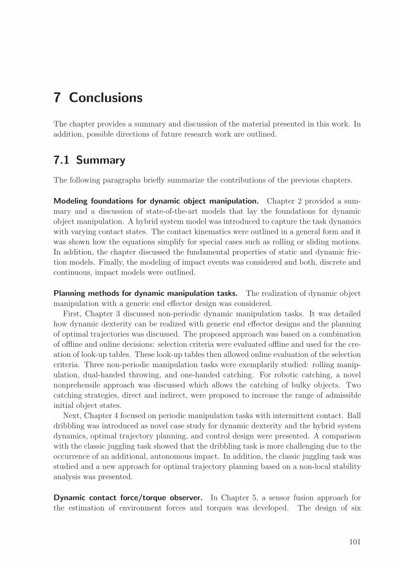
7 Conclusions
The chapter provides a summary and discussion of the material presented in this work. In
addition, possible directions of future research work are outlined.
7.1 Summary
The following paragraphs briefly summarize the contributions of the previous chapters.
Modeling foundations for dynamic object manipulation. Chapter 2 provided a sum-
mary and a discussion of state-of-the-art models that lay the foundations for dynamic
object manipulation. A hybrid system model was introduced to capture the task dynamics
with varying contact states. The contact kinematics were outlined in a general form and it
was shown how the equations simplify for special cases such as rolling or sliding motions.
In addition, the chapter discussed the fundamental properties of static and dynamic fric-
tion models. Finally, the modeling of impact events was considered and both, discrete and
continuous, impact models were outlined.
Planning methods for dynamic manipulation tasks. The realization of dynamic object
manipulation with a generic end effector design was considered.
First, Chapter 3 discussed non-periodic dynamic manipulation tasks. It was detailed
how dynamic dexterity can be realized with generic end effector designs and the planning
of optimal trajectories was discussed. The proposed approach was based on a combination
of offline and online decisions: selection criteria were evaluated offline and used for the cre-
ation of look-up tables. These look-up tables then allowed online evaluation of the selection
criteria. Three non-periodic manipulation tasks were exemplarily studied: rolling manip-
ulation, dual-handed throwing, and one-handed catching. For robotic catching, a novel
nonprehensile approach was discussed which allows the catching of bulky objects. Two
catching strategies, direct and indirect, were proposed to increase the range of admissible
initial object states.
Next, Chapter 4 focused on periodic manipulation tasks with intermittent contact. Ball
dribbling was introduced as novel case study for dynamic dexterity and the hybrid system
dynamics, optimal trajectory planning, and control design were presented. A comparison
with the classic juggling task showed that the dribbling task is more challenging due to the
occurrence of an additional, autonomous impact. In addition, the classic juggling task was
studied and a new approach for optimal trajectory planning based on a non-local stability
analysis was presented.
Dynamic contact force/torque observer. In Chapter 5, a sensor fusion approach for
the estimation of environment forces and torques was developed. The design of six
101

7 Conclusions
DOF force/torque observers based on the EKF and on the UKF was discussed. For
both approaches, two measurement vectors were considered: the first one used pose and
force/torque measurements while the second one also used acceleration and velocity mea-
surements. The four filter designs were evaluated in a six DOF simulation scenario and
in experiments. The obtained results illustrated the importance of such an observer, not
only for dynamic object manipulation but also for other tasks that require environment
interaction during dynamic motions. With the quantitative comparisons, the appropriate
observer design can be chosen according to the task-specific requirements.
Control framework for dynamic object manipulation. Chapter 5 also addressed the
challenges for the closed-loop control of dynamic manipulation tasks and presented an ex-
tensive control framework to overcome these challenges. With respect to environment per-
ception, a method for high-speed image processing was presented. This allows to track and
to predict the state of manipulated objects during non-contact phases with high sampling
rates. Together with the dynamic force/torque observer, the high-speed image processing
was integrated into the control architecture and used for the robot action planning. In
addition, the motion and interaction control was discussed. The force/torque observer
was integrated in a direct force control scheme to improve the interaction control during
dynamic motions.
Dynamic manipulation with a compliant end effector. The thesis considered the con-
cept of series elastic actuation to improve the performance in dynamic manipulation tasks.
While such an approach adds complexity to the task planning, it also promises several
beneficial effects: first, kinetic energy of the object can be transformed in potential energy
of the spring element. This relaxes the acceleration requirements for the manipulator and
facilitates the task execution. Second, the elastic element reduces the mechanical load for
the manipulator at impact events as it establishes a continuous-time contact phase which
replaces the impulsive contact force of an instantaneous impact. Finally, the continuous-
time contact phase extends the time in which the object can be directly controlled with
the manipulator. The approach was evaluated in experiments: the dribbling task was
performed with both, a compliant and a rigid end effector design. Their comparison con-
firmed the expected benefits and provides a basis for further development of the mechanical
design.
Experimental evaluation. In Chapter 6, nonprehensile catching, throwing, dribbling,
and juggling tasks were experimentally studied with a six DOF industrial robot and a 14
DOF anthropomorphic dual-arm manipulator. The experiments validated the approach
of the thesis by integrating the results with respect to modeling, environment perception,
planning and control design in a robotic basketball scenario. In addition, the experiments
provided valuable insights into practical issues that had not been considered in the theo-
retical analysis.
102

7.2 Discussion and Future Directions
7.2 Discussion and Future Directions
Individual aspects of the topics presented in this thesis were discussed at the end of each
chapter. This section comments on the most important issues and outlines possible im-
provements and extensions for future research.
Mechanical design. The occurrence of motion sequences with high manipulator acceler-
ation is a characteristic feature of dynamic object manipulation. Consequently, an increase
of the peak power is desirable. One way to realize this is the use of motors with higher
output power. However, this is not reasonable since size and weight of a humanoid or
autonomous robot are usually constrained and, in addition, a temporary increase is suf-
ficient. Hence, the concept of series elastic actuation was employed in this work. The
benefits were exemplarily demonstrated by comparing the dribbling task with a rigid and
a compliant end effector design. On the one hand, the results emphasized the importance
of the mechanical design for the planning and execution of dynamic manipulation tasks.
On the other hand, the experiments showed that the optimal stiffness is task-dependent
and can even change for different phases of a particular task. Thus, a manipulator design
with variable stiffness actuation (VSA) is desirable to further improve the system perfor-
mance. Such an adjustable stiffness is also beneficial for manipulation tasks that include
a physical human-robot interaction.
Manipulation of elastic and arbitrarily shaped objects. The manipulated objects in
this work were effectively rigid, compare Sec. 2.6. This allowed the use of discrete impact
models and hence simplified the task planning and trajectory optimization. For the plan-
ning of dynamic manipulation tasks with elastic objects, continuous or distributed models
are needed. Furthermore, the applications and case studies in this work considered the
manipulation of spherical objects. Thus, the object orientation did not influence the task
planning. The manipulation of non-spherical objects generally implies preferred orienta-
tions and hence poses additional challenges for both task planning and object tracking.
Multi-camera system. In this work, a stereo camera system was utilized to provide visual
feedback of the environment. With this approach, an occlusion of the object in one camera
results in a loss of 3D information. In order to address this problem, future research work
could focus on a multi-camera setup that allows robust tracking of the object at high frame
rates. Another important criteria for successful task execution is the field of view of the
cameras, compare Sec. 6.3. With a multi-camera system, different field of views can be
fused to obtain a thorough visual perception of the environment.
Library of dynamic manipulation skills. The planning and control methods presented in
this work were applied to a number of case studies. However, the modeling foundations, the
planning approach, and the overall control structure can be used for a wide range of tasks
which require a dynamically dexterous robot. Hence, by building upon this framework,
future research work can establish a library of dynamic manipulation skills.
103

7 Conclusions
Dynamic manipulation with multi-fingered robotic hands. This work considered the
realization of dynamic manipulation tasks with simple end effector designs. Such an ap-
proach is desirable as it generalizes to more complex hands, e.g. when only the palm
of a multi-fingered hand is used for a particular task. However, dynamic dexterity and
multi-fingered hands clearly do not exclude each other. On the contrary, some dynamic
manipulation tasks even require hands with multiple DOF, e.g. twisting a pen in one’s
hand. Realizing dynamic object manipulation with a multi-fingered hand is one of the
future milestones for robotic manipulation.
104

A Appendix
A.1 Differential Geometry
Detailed information on the following terms can be found in the in the books by DoCarmo
and Murray [34, 92].
First fundamental form. For a surface, the first fundamental form describes how the
inner product of two tangent vectors is related to the natural inner product on R3. For a
local parameterization c(u, v), the matrix representation of the first fundamental form at
a point p is given by
Ip =
[
cTucu cTucvcTv cu cTv cv
]
. (A.1)
Metric tensor. The metric tensor of a surface is given by the square root of the first
fundamental form
Ip = M pM p. (A.2)
For an orthogonal parameterization, M p takes the form
M p =
[
||cu|| 0
0 ||cv||
]
. (A.3)
Outward pointing unit normal vector. The vector
n(u, v) =cu × cv
||cu × cv||(A.4)
denotes the unit normal at a point of the surface.
Second fundamental form. For a surface, the second fundamental form is defined as
IIp =
[
cTu nu cTu nv
cTv nu cTv nv
]
. (A.5)
Curvature tensor. For an orthogonal parameterization, the curvature tensor is defined
as
Kp = M−Tp IIpM
−1p =
[
cTu nu
||cu||2
cTu nv
||cu||||cv ||cTv nu
||cu||||cv ||cTv nv
||cv ||2
]
. (A.6)
105

A Appendix
Torsion form. The torsion of a surface is a measure of how the Gauss frame twists when
moving across the surface. It is defined as
T p =[
cTv cuu
||cu||2||cv ||
cTv cuv
||cu||||cv ||2
]
. (A.7)
Geometric parameters of a surface. For a given parameterization, the collective of the
metric tensor M , the curvature K, and the torsion form T are the geometric parameters
of the surface.
A.2 Velocity and Force/Torque Transformations
Velocity transformation. The velocities of two points A and C fixed on a rigid body are
related according to the following relation
r0C =r0
A + ω0A × r0
AC (A.8)
ω0C =ω0
A, (A.9)
or in matrix notation[
r0C
ω0C
]
=
[
I −S(r0AC)
0 I
] [
r0A
ω0A
]
. (A.10)
When the velocities are referred to their own frames one obtains[
rCCωCC
]
=
[
RCA −RC
AS(rAAC)
0 RCA
] [
rAAωAA
]
. (A.11)
Here, the subscripts A and C for ω can be omitted since the rotational velocity is identical
for every point on the rigid body.
Force/Torque transformation. The forces and torques applied on a rigid body at point
A can be transformed to corresponding forces and torques at a different reference point C
inertial frame Σ0
ΣA
ΣCrA
rC
rAC
Fig. A.1: Representation of velocities in different coordinate frames.
106

A.3 Orientation of a Rigid Body: Unit Quaternion
according to
[
F 0C
M 0C
]
=
[
I 0
S(r0CA) I
] [
F 0A
M 0A
]
. (A.12)
When the forces and torques are referred to their own frames one obtains
[
F CC
MCC
]
=
[
RCA 0
S(rCCA)RCA RC
A
] [
F AA
MAA
]
. (A.13)
In some cases, however, it will be helpful to illustrate the origin of the transformed forces
and torques. Then, the following extended notation is used
[
F CA→B
MCA→B
]
, (A.14)
which means the forces and torques applied at point A have been transformed to the
corresponding forces and torques at point B and are expressed in frame C.
A.3 Orientation of a Rigid Body: Unit Quaternion
This section outlines the use of unit quaternions to describe the orientation of a rigid body.
A detailed discussion on unit quaternions and on other generalized coordinates for the
orientation of a rigid body can be found in the books by Wittenburg and Natale [145, 94].
Skew-symmetric operator. The skew-symmetric operator is defined as
S (r) =
0 −rz ryrz 0 −rx−ry rx 0
. (A.15)
Unit quaternion. The unit quaternion is defined as
o = η, ǫ , (A.16)
where η is the scalar part and ǫ = [ǫx ǫy ǫz]T is the vector part of the quaternion. The
unit quaternion fulfills the condition
||o||2 = η2 + ǫTǫ = η2 + ǫ2x + ǫ2y + ǫ2z = 1. (A.17)
The inverse of the unit quaternion is given by
o−1 = η,−ǫ . (A.18)
107

A Appendix
The quaternion product operation is defined as
o1 ∗ o2 =
[
η1η2 − ǫT1 ǫ2η1ǫ2 + η2ǫ1 + S (ǫ1) ǫ2
]
. (A.19)
Angular velocity. An expression for the angular velocity can be derived based on (A.19).
Starting with an initial orientation o10 at time t, the rotation o20 is interpreted as a
differential rotation over the time interval dt,
o20 = η20, ǫ20 =
cos
(
1
2||ω|| dt
)
,ω
||ω||sin
(
1
2||ω|| dt
)
. (A.20)
For dt→ 0, o20 =
1, 12ω
and (A.19) can be rewritten as
η(t+ dt) =η10(t)−1
2ǫ10(t)
Tωdt, (A.21)
ǫ(t+ dt) =ǫ10(t) +1
2[η10(t)ω + S (ω) ǫ10(t)] dt. (A.22)
This yields to the so called unit quaternion propagation
η10 =−1
2ǫT10ω10, (A.23)
ǫ10 =1
2[η10I − S (ǫ10)]ω10. (A.24)
A.4 Newton-Euler Equations for a Rigid Body
For a reference point A fixed on the rigid body and an inertial frame Σ0 as reference frame,
the Newton-Euler equations for a rigid body are given by [145]
F A = mrA −mS (rAC)ω +mω × (ω × rAC)
MA = mrAC × rA + JAωA + ωA × JAωA (A.25)
If the reference point A coincides with the center of mass rAC = 0, (A.25) simplifies to
F A = mrA
MA = JAωA + ωA × JAωA (A.26)
Inertia tensor. The inertia tensor of a rigid body with respect to a body-fixed reference
point A and expressed in the inertial frame Σ0 is given by
JA = J0A. (A.27)
If the rigid body is rotating, the inertia tensor expressed in the inertial frame is time-
varying. A constant expression for the inertia tensor is obtained by choosing a body-fixed
108
A.4 Newton-Euler Equations for a Rigid Body
reference frame, such as a frame ΣC located at the center of mass (COM),
JCA. (A.28)
For a constant reference point A, a change of the reference frame for the inertia tensor is
realized by
JCA = RC
B JBA RB
C . (A.29)
109

Bibliography
[1] SMErobot - The European Robot Initiative for Strengthening the Competitiveness
of SMEs in Manufacturing. http://www.smerobot.org, 2011.
[2] E.W. Aboaf, S.M. Drucker, and C.G. Atkeson. Task-level robot learning: Juggling
a tennis ball more accurately. In Proc. IEEE International Conference on Robotics
and Automation (ICRA), pages 1290 – 1295, 1989.
[3] R.L. Andersson. Dynamic sensing in a ping-pong playing robot. IEEE Transactions
on Robotics and Automation, 5(6):728–739, 1989.
[4] B. Armstrong-Helouvry, P. Dupont, and C. Canudas de Wit. A survey of models,
analysis tools and compensation methods for the control of machines with friction.
Automatica, 30(7):1083 –1138, 1994.
[5] C. N. Bapat, S. Sankar, and N. Popplewell. Repeated impacts on a sinusoidally
vibrating table reappraised. Journal of Sound and Vibration, 108(1):99–115, 1986.
[6] B. Bauml, T. Wimbock, and G. Hirzinger. Kinematically optimal catching a fly-
ing ball with a hand-arm-system. In Proc. IEEE/RSJ International Conference on
Intelligent Robots and Systems (IROS), pages 2592–2599, 2010.
[7] L. Biagiotti and C. Melchiorri. Advances in Telerobotics, chapter Environment Es-
timation in Teleoperation Systems, pages 211–232. Springer (Berlin / Heidelberg),
2007.
[8] A. Bicchi. Hands for dexterous manipulation and robust grasping: A difficult road
towards simplicity. IEEE Transactions on Robotics and Automation, 16(6):652–662,
2000.
[9] A. Bicchi and V. Kumar. Robotic grasping and contact: a review. In Proc. IEEE
International Conference on Robotics and Automation (ICRA), pages 348–353, 2000.
[10] A. Bicchi and V. Kumar. Lecture Notes in Control and Information Science, chapter
Robot Grasping and Manipulation, pages 55–74. Springer (Berlin / Heidelberg),
2001.
[11] A. Bicchi and A. Marigo. Rolling contacts and dexterous manipulation. In Proc.
IEEE International Conference on Robotics and Automation (ICRA), pages 282–287,
2000.
[12] A. Bicchi, D. Prattichizzo, and S. Sastry. Planning motions of rolling surfaces. In
Proc. IEEE Conference on Decision and Control (CDC), pages 2812–2817, 1995.
110
[13] P.-A. Bliman and M. Sorine. Easy-to-use realistic dry friction models for automatic
control. In Proc. European Control Conference (ECC), pages 3788–3794, 1995.
[14] B. Bona and M. Indri. Friction compensation in robotics: an overview. In Proc.
IEEE Conference on Decision and Control (CDC), pages 4360–4367, 2005.
[15] R. M. Brach. Formulation of rigid body impact problems using generalized coeffi-
cients. International Journal of Engineering Science, 36(1):61–71, 1998.
[16] M. S. Branicky, V. S. Borkar, and S. K. Mitter. A unified framework for hybrid con-
trol: model and optimal control theory. IEEE Transactions on Automatic Control,
43(1):31–45, 1998.
[17] R. Brockett. Essays on Control: Perspectives in the Theory and its Applications,
chapter Hybrid models for motion control systems, pages 29–53. Birkhauser (Basel),
1993.
[18] B. Brogliato. Nonsmooth Mechanics - Models, Dynamics, and Control. Springer
(Berlin / Heidelberg), 1999.
[19] B. Brogliato and A. Zavalo-Rio. On the control of complementary-slackness juggling
mechanical systems. IEEE Transactions on Automatic Control, 45(2):235–246, 2000.
[20] M. Buhler, D.E. Koditschek, and P.J. Kindlmann. A one degree of freedom juggler
in a two degree of freedom environment. In Proc. IEEE International Workshop on
Intelligent Robots, pages 91–97, 1988.
[21] M. Buhler, D.E. Koditschek, and P.J. Kindlmann. A family of robot control strategies
for intermittent dynamical environments. IEEE Control Systems Magazine, 10(2):16–
22, 1990.
[22] M. Buhler, D.E. Koditschek, and P.J. Kindlmann. Planning and control of robotic
juggling and catching tasks. International Journal of Robotics Research, 13(2):101–
118, 1994.
[23] R. R. Burridge, A. A. Rizzi, and D. E. Koditschek. Sequential composition of dy-
namically dexterous robot behaviors. International Journal of Robotics Research,
18(6):534–555, 1999.
[24] R.R. Burridge, A.A. Rizzi, and D.E. Koditschek. Toward a dynamical pick and
place. In Proc. IEEE/RSJ International Conference on Intelligent Robots and Sys-
tems (IROS), pages 292–297, 1995.
[25] M. Buss. Methoden zur Regelung Hybrider Dynamischer Systeme - Modelle,
Regelkreise, Optimalsteuerung, Rechnerwerkzeuge und Mechatronik-Anwendungen.
Habilitationsschrift, 2000.
[26] F. Caccavale, C. Natale, B. Siciliano, and L. Villani. Six-dof impedance control
based on angle/axis representations. IEEE Transactions on Robotics and Automa-
tion, 15(2):289–300, 1999.
111

Bibliography
[27] C. Canudas de Wit, H. Olsson, K. J. Astrom, and P. Lischinsky. A new model for con-
trol of systems with friction. IEEE Transactions on Automatic Control, 40(3):419–
425, 1995.
[28] S. Chiaverini and L. Sciavicco. The parallel approach to force/position control of
robotic manipulators. IEEE Transactions on Robotics and Automation, 9(4):361–
373, 1993.
[29] S. Chiaverini, B. Siciliano, and L. Villani. A survey of robot interaction control
schemes with experimental comparison. 4(3):273–285, 1999.
[30] E. Coumans. The bullet physics simulation toolkit. www.bulletphysics.com.
[31] R. Cross. Grip-slip behavior of a bouncing ball. American Journal of Physics,
11:1093–1102, 2002.
[32] P. R. Dahl. Solid friction damping of mechanical vibrations. In Proc. AIAA Guidance
and Control Conference, 1976.
[33] N. Diolaiti, C. Melchiorri, and S. Stramigioli. Contact impedance estimation for
robotic systems. IEEE Transactions on Robotics, 21(5):925–935, 2005.
[34] M. P. do Carmo. Differential Geometry of Curves and Surfaces. Prentice-Hall (New
Jersey), 1976.
[35] A. Domenech. A classical experiment revisited: The bounce of balls and superballs
in three dimensions. American Journal of Physics, 1:28–36, 2005.
[36] M. A. Erdmann. exploration of nonprehensile two-palm manipulation: Planning and
execution. In International Symposium on Robotics Research, 1995.
[37] H. Frank, D. Barteit, N. Wellerdick-Wojtasik, T. Frank, G. Novak, and
S. Mahlknecht. Autonomous mechanical controlled grippers for capturing flying
objects. In Proc. IEEE International Conference on Industrial Informatics, pages
431–436, 2007.
[38] U. Frese, B. Bauml, S. Haidacher, G. Schreiber, I. Schafer, M. Hahnle, and
G. Hirzinger. Off-the-shelf vision for a robotic ball catcher. In Proc. IEEE/RSJ
International Conference on Intelligent Robots and Systems (IROS), pages 1623–
1629, 2001.
[39] N. Furukawa, A. Namiki, S. Taku, and M. Ishikawa. Dynamic regrasping using
a high-speed multifingered hand and a high-speed vision system. In Proc. IEEE
International Conference on Robotics and Automation (ICRA), pages 181–187, 2006.
[40] M. Gafvert. Comparisons of two dynamic friction models. In Proc. IEEE Interna-
tional Conference on Control Applications, 1997.
[41] J. A. Gangloff and M. F. de Mathelin. High-speed visual servoing of a 6-d.o.f.
manipulator using multivariable control. Advanced Robotics, 17(10):993–1021, 2003.
112
[42] J. Garcia, A. Robertsson, J. Ortega, and R. Johansson. Generalized contact force es-
timator for a robot manipulator. In Proc. IEEE International Conference on Robotics
and Automation (ICRA), pages 4019–4024, 2006.
[43] J.G. Garcia, A. Robertsson, J.G. Ortega, and R. Johansson. Sensor fusion for com-
pliant robot motion control. IEEE Transactions on Robotics, 24(2):430–441, 2008.
[44] K. J. Gergen and M. M. Gergen. Social Psychology. Springer (Berlin / Heidelberg),
1986.
[45] G. Gilardi and I. Sharf. Literature survey of contact dynamics modelling. Mechanism
and Machine Theory, 37(10):1213–1239, 2002.
[46] C. Glocker. Dynamik von Starrkorpersystemen mit Reibung und Stoßen. PhD thesis,
Technische Universitat Munchen, 1995.
[47] A. Haddadi and K. Hashtrudi-Zaad. A new method for online parameter estimation
of hunt-crossley environment dynamic models. In Proc. IEEE/RSJ International
Conference on Intelligent Robots and Systems (IROS), pages 981–986, 2008.
[48] D. Haessig and B. Friedland. On the modeling and simulation of friction. In Proc.
American Control Conference (ACC), pages 1256 –1261, 1990.
[49] R. M. Haralick and L. G. Shapiro. Computer and Robot Vision. Addison-Wesley,
2002.
[50] H. Hertz. Uber die Beruhrung fester elastischer Korper. Journal fur die reine und
angewandte Mathematik, 92:156–171, 1881.
[51] I. Hiskens. Stability of hybrid system limit cycles: Application to the compass gait
biped robot. In Proc. IEEE Conference on Decision and Control (CDC), pages
774–779, 2001.
[52] J. Hodgins and M. Raibert. Biped gymnastics. International Journal of Robotics
Research, 9:115–128, 1990.
[53] N. Hogan. Impedance control: An approach to manipulation. In Proc. American
Control Conference (ACC), pages 304–313, 1984.
[54] P. J. Holmes. The dynamics of repeated impacts with a sinusoidally vibrating table.
Journal of Sound and Vibration, 84(2):173–189, 1982.
[55] B. Hove and J.-J. Slotine. Experiments in robotic catching. In Proc. American
Control Conference (ACC), pages 380–386, 1991.
[56] C. S. Hsu. Global analysis by cell mapping. International Journal of Bifurcation and
Chaos, 2(4):727–771, 1992.
[57] W. Huang. Impulsive Manipulation. PhD thesis, Carnegie Mellon University, 1997.
113

Bibliography
[58] K. H. Hunt and F. R. E. Crossley. Coefficient of restitution interpreted as damping
in vibroimpact. ASME Journal of Applied Mechanics, 42(2):440–445, 1975.
[59] Y. Imai, A. Namiki, K. Hashimoto, and M. Ishikawa. Dynamic active catching using
a high-speed multifingered hand and a high-speed vision system. In Proc. IEEE
International Conference on Robotics and Automation (ICRA), pages 1849–1854,
2004.
[60] E. A. Jackson. Perspectives of Nonlinear Dynamics, volume 1. Cambridge University
Press (Cambridge), 1989.
[61] H.-L. Jin, Q. Ye, and M. Zacksenhouse. Return maps, parameterization, and cycle-
wise planning of yo-yo playing. IEEE Transactions on Robotics, 25(2):438–445, 2009.
[62] H.-L. Jin and M. Zacksenhouse. Oscillatory neural networks for robotic yo-yo control.
IEEE Transactions on Neural Networks, 14(2):317–325, 2003.
[63] H.-L. Jin and M. Zacksenhouse. Robotic yoyo playing with visual feedback. IEEE
Transactions on Robotics, 20(4):736–744, 2004.
[64] S. J. Julier and J. K. Uhlmann. A new extension of the kalman filter to nonlinear
systems. Technical report, The Robotics Research Group, Department of Engineering
Science, The University of Oxford, 1997.
[65] S. J. Julier and J. K. Uhlmann. Unscented filtering and nonlinear estimation. Pro-
ceedings Of the IEEE, 92(3):401–422, 2004.
[66] S. J. Julier, J. K. Uhlmann, and H. F. Durrant-Whyte. A new approach for filtering
nonlinear systems. In Proc. American Control Conference (ACC), pages 1628–1632,
1995.
[67] N. Kato, K. Matsuda, and T. Nakamura. Adaptive control for a throwing motion of
a 2 dof robot. In Proc. International Workshop on Advanced Motion Control, pages
203–207, 1996.
[68] S. Katsumata, S. Ichinose, T. Shoji, S. Nakaura, and M. Sampei. Throwing mo-
tion control based on output zeroing utilizing 2-link underactuated arm. In Proc.
American Control Conference (ACC), pages 3057–3064, 2009.
[69] H. K. Khalil. Nonlinear Systems. Prentice-Hall (New Jersey), 2000.
[70] O. Khatib. A unified approach for motion and force control of robot manipulators:
The operational space formulation. IEEE Journal on Robotics and Automation,
3(1):43–53, 1987.
[71] D. Koditschek. Robot Control: Dynamics, Motion Planning and Analysis, chapter
Dynamically dexterous robots. IEEE Press, 1993.
[72] I. Kolmanovsky and N. H. McClamroch. Developments in nonholonomic control
problems. IEEE Control Systems Magazine, 15(6):20–36, 1995.
114

[73] E. Kraft. A quaternion-based unscented kalman filter for orientation tracking. In
Proc. IEEE International Conference of Information Fusion, pages 47–54, 2003.
[74] T. Kroger, D. Kubus, and F.M. Wahl. 6d force and acceleration sensor fusion for
compliant manipulation control. In Proc. IEEE/RSJ International Conference on
Intelligent Robots and Systems (IROS), pages 2626–2631, 2006.
[75] D. Kubus, T. Kroger, and F.M. Wahl. Improving force control performance by com-
putational elimination of non-contact forces/torques. In Proc. IEEE International
Conference on Robotics and Automation (ICRA), pages 2617–2622, 2008.
[76] H. Lankarani and P. Nikravesh. Continuous contact force models for impact analysis
in multibody systems. Nonlinear Dynamics, 5(2):193–207, 1994.
[77] H. E. Lehtitet and B. N. Miller. Numerical study of a billiard in a gravitational field.
Physica, 21(1):93–104, 1986.
[78] S.-T. Lin. Force sensing using kalman filtering techniques for robot compliant motion
control. Journal of Intelligent and Robotic Systems, 18(1):1–16, 1997.
[79] F. Lombai and G. Szederkenyi. Throwing motion generation using nonlinear opti-
mization on a 6-degree-of-freedom robot manipulator. In Proc. IEEE International
Conference on Mechatronics, pages 1–6, 2009.
[80] A. Luo and R. Han. The dynamics of a bouncing ball with a sinusoidally vibrating
table revisited. Nonlinear Dynamics, 10(1):1–18, 1996.
[81] K. M. Lynch and C. K. Black. Recurrence, controllability and stability of juggling.
IEEE Transaction on Robotics and Automation, 17(2):113–124, 2001.
[82] K. M. Lynch and M. T. Mason. Dynamic underactuated nonprehensile manipula-
tion. In Proc. IEEE/RSJ International Conference on Intelligent Robots and Systems
(IROS), pages 889–896, 1996.
[83] K. M. Lynch and M. T. Mason. Dynamic manipulation with a one joint robot. In
Proc. IEEE International Conference on Robotics and Automation (ICRA), pages
359–366, 1997.
[84] K. M. Lynch and M. T. Mason. Dynamic nonprehensile manipulation: Controllabil-
ity, planning, and experiments. International Journal of Robotics Research, 18(1):64–
92, 1999.
[85] K. M. Lynch, N. Shiroma, H. Arai, and K. Tanie. The roles of shape and mo-
tion in dynamic manipulation: the butterfly example. In Proc. IEEE International
Conference on Robotics and Automation (ICRA), pages 1958–1963, 1998.
[86] D. W. Marhefka and D. E. Orin. A compliant contact model with nonlinear damp-
ing for simulation of robotic systems. IEEE Transactions on Systems, Man and
Cybernetics, 29(6):566–572, 1999.
115
Bibliography
[87] A. Marigo and A. Bicchi. Rolling bodies with regular surface: Controllability theory
and applications. IEEE Transactions on Automatic Control, 45(9):1586–1599, 2000.
[88] M. Mason. Mechanics of Robotic Manipulation. MIT Press, 2001.
[89] M. T. Mason. Progress in nonprehensile manipulation. International Journal of
Robotics Research, 18(11):1129–1141, 1999.
[90] M.T. Mason and K.M. Lynch. Dynamic manipulation. In Proc. IEEE/RSJ Interna-
tional Conference on Intelligent Robots and Systems (IROS), pages 152–159, 1993.
[91] D. J. Montana. The kinematics of contact and grasp. International Journal of
Robotics Research, 7:17–32, 1989.
[92] R. M. Murray, Z. Li, and S. Sastry. A Mathematical Introduction to Robotic Manip-
ulation. CRC Press (Boca Raton), 1994.
[93] A. Namiki, K. Hashimoto, and M. Ishikawa. A hierarchical control architecture for
high-speed visual servoing. International Journal of Robotics Research, 22:873–888,
2004.
[94] C. Natale. Interaction Control of Robot Manipulators - Six-Degrees-of-Freedom
Tasks. Springer (Berlin / Heidelberg), 2003.
[95] A. M. Okamura, N. Smaby, and M. R. Cutkosky. An overview of dexterous ma-
nipulation. In Proc. IEEE International Conference on Robotics and Automation
(ICRA), pages 255 – 262, 2000.
[96] H. Olsson and K. J. Astrom. Observer-based friction compensation. In Proc. IEEE
Conference on Decision and Control (CDC), pages 4345–4350, 1996.
[97] H. Olsson, K. J. Astrom, C. Canudas de Wit, M. Gafvert, and P. Lischinsky. Friction
models and friction compensation. European Journal of Control, 4(3):176–195, 1998.
[98] G. Oriolo, M. Vendittelli, A. Marigo, and A. Bicchi. From nominal to robust planning:
The plate-ball manipulation system. In Proc. IEEE International Conference on
Robotics and Automation (ICRA), pages 3175–3180, 2003.
[99] T. S. Parker and L. O. Chua. Practical Numerical Algorithms for Chaotic Systems.
Springer (Berlin / Heidelberg), 1989.
[100] F. Pfeiffer and C. Glocker. Multibody Dynamics with Unilateral Contacts. Wiley-
VCH (Weinheim), 2004.
[101] M. H. Raibert and J. J. Craig. Hybrid position/force control of manipulators. ASME
Journal of Dynamic Systems, Measurement, and Control, 103(2):126–133, 1981.
[102] P. Reist and R. D’Andrea. Bouncing an unconstrained ball in three dimensions with
a blind juggling robot. In Proc. IEEE International Conference on Robotics and
Automation (ICRA), pages 1774–1781, 2009.
116

[103] M. Riley and C.G. Atkeson. Robot catching: Towards engaging human-humanoid
interaction. Autonomous Robots, 12(1):119–128, 2002.
[104] A. A. Rizzi and D. E. Koditschek. Progress in spatial robot juggling. In Proc. IEEE
International Conference on Robotics and Automation (ICRA), pages 775–780, 1992.
[105] A. A. Rizzi and D. E. Koditschek. Further progress in robot juggling: the spatial
two-juggle. In Proc. IEEE International Conference on Robotics and Automation
(ICRA), pages 919–924, 1993.
[106] A. A. Rizzi and D. E. Koditschek. Toward the control of attention in a dynamically
dexterous robot. In Proc. IEEE/RSJ International Conference on Intelligent Robots
and Systems (IROS), pages 123–130, 1993.
[107] A. A. Rizzi and D. E. Koditschek. Further progress in robot juggling: solvable mirror
laws. In Proc. IEEE International Conference on Robotics and Automation (ICRA),
pages 2935–2940, 1994.
[108] R. Ronsse, P. Lefevre, and R. Sepulchre. Open-loop stabilization of 2d impact jug-
gling. In Proc. IFAC Symposium on Nonlinear Control Systems, pages 1157–1162,
2004.
[109] R. Ronsse, P. Lefevre, and R. Sepulchre. Timing feedback control of a rhythmic
system. In Proc. IEEE Conference on Decision and Control and the European Control
Conference (CDC-ECC), pages 6146–6151, 2005.
[110] R. Ronsse, P. Lefevre, and R. Sepulchre. Sensorless stabilization of bounce juggling.
IEEE Transactions on Robotics, 22(1):147–159, 2006.
[111] R. Ronsse, P. Lefevre, and R. Sepulchre. Rhythmic feedback control of a blind planar
juggler. IEEE Transactions on Robotics, 23(4):790–802, 2007.
[112] R. Ronsse and R. Sepulchre. Feedback control of impact dynamics: the bouncing
ball revisited. In Proc. IEEE Conference on Decision and Control (CDC), pages
4807–4812, 2006.
[113] T. Sakaguchi, Y. Masutani, and F. Miyazaki. A study on juggling task. In Proc.
IEEE/RSJ International Conference on Intelligent Robots and Systems (IROS),
1991.
[114] S. Schaal and C. G. Atkeson. Open loop stable control strategies for robot juggling.
In Proc. IEEE International Conference on Robotics and Automation (ICRA), pages
913–918, 1993.
[115] S. Schaal and C. G. Atkeson. Memory-based robot learning. In Proc. IEEE In-
ternational Conference on Robotics and Automation, pages 2928–2933, 8–13 May
1994.
[116] S. Schaal and C. G. Atkeson. Robot juggling: implementation of memory-based
learning. IEEE Control Systems Magazine, 14(1):57–71, 1994.
117
Bibliography
[117] S. Schaal, D. Sternad, and C. G. Atkeson. One-handed juggling: A dynamical
approach to a rhythmic movement task. Journal of Motor Behavior, 28(2):165–183,
1996.
[118] A. L. Schwab and M. Wisse. Basin of attraction of the simplest walking model. In
Proc. ASME Design Engineering Technical Conferences and Computers and Infor-
mation in Engineering Conference, pages 1–9, 2001.
[119] T. Senoo, A. Namiki, and M. Ishikawa. Ball control in high-speed batting motion us-
ing hybrid trajectory generator. In Proc. IEEE International Conference on Robotics
and Automation (ICRA), pages 1762–1767, 2006.
[120] T. Senoo, A. Namiki, and M. Ishikawa. High-speed throwing motion based on kinetic
chain approach. In Proc. IEEE/RSJ International Conference on Intelligent Robots
and Systems (IROS), pages 3206–3211, 2008.
[121] R. Sepulchre and M. Gerard. Stabilization of periodic orbits in a wedge billiard. In
Proc. IEEE Conference on Decision and Control (CDC), volume 2, pages 1568–1573,
2003.
[122] D. Shiokata, A. Namiki, and M. Ishikawa. Robot dribbling using a high-speed mul-
tifingered hand and a high-speed vision system. In Proc. IEEE/RSJ International
Conference on Intelligent Robots and Systems (IROS), pages 2097–2102, 2005.
[123] A. Shiriaev, L. Freidovich, and S. Gusev. Transverse linearization for controlled
mechanical systems with several passive degrees of freedom. IEEE Transactions on
Automatic Control, 55:1–13, 2010.
[124] A. Shiriaev, L. Freidovich, and I. Manchester. Periodic motion planning and analyt-
ical computation of transverse linearizations for hybrid mechanical systems. In Proc.
IEEE Conference on Decision and Control (CDC), pages 4326–4331, 2008.
[125] B. Siciliano and O. Khatib, editors. Springer Handbook of Robotics. Springer (Berlin
/ Heidelberg), 2008.
[126] B. Siciliano, L. Sciavicco, L. Villani, and G. Oriolo. Robotics - Modelling, Planning
and Control. Springer (Berlin / Heidelberg), 2008.
[127] S. N. Simic, K. Johansson, J. Lygeros, and S. Sastry. Towards a geometric theory
of hybrid systems. Dynamics of Continuous, Discrete and Impulsive Systems, Series
B, 12(5-6):649–687, 2005.
[128] S. N. Simic, K. H. Johansson, J. Lygeros, and S. Sastry. Structural stability of hybrid
systems. In Proc. European Control Conference (ECC), pages 3858–3863, 2001.
[129] J.-J. Slotine and W. Li. Applied Nonlinear Control. Prentice-Hall (New Jersey),
1991.
[130] M. Sobotka. Hybrid Dynamical System Methods for Legged Robot Locomotion with
Variable Ground Contact. PhD thesis, Technische Universitat Munchen, 2007.
118

[131] M. W. Spong. Partial feedback linearization of underactuated mechanical systems.
In Proc. IEEE/RSJ International Conference on Intelligent Robots and Systems
(IROS), pages 314–321, 1994.
[132] B. Stanczyk. Development and Control of an Anthropomorphic Telerobotic System.
PhD thesis, Technische Universitat Munchen, 2006.
[133] D. Sternad, M. Duarte, H. Katsumata, and S. Schaal. Dynamics of a bouncing ball
in human performance. Phys. Rev. E, 63(1):011902, 2000.
[134] D. Sternad, M. Duarte, H. Katsumata, and S. Schaal. Bouncing a ball: Tuning
into dynamic stability. Journal of Experimental Psychology: Human Perception and
Performance, 27(5):1163–1184, 2001.
[135] R. Stribeck. Die wesentlichen Eigenschaften der Gleit- und Rollenlager. Zeitschrift
des Vereins Deutscher Ingenieure, 46:1341–1348, 1902.
[136] W. J. Stronge. Rigid body collisions with friction. Mathematical and Physical Sci-
ences, 431(1881):169–181, 1990.
[137] C. Studer. Augmented time-stepping integration of non-smooth dynamical systems.
PhD thesis, ETH Zurich, 2008.
[138] J. Tian and Y.-B. Jia. Modeling deformable shell-like objects grasped by a robot
hand. In Proc. IEEE International Conference on Robotics and Automation (ICRA),
pages 1297–1302, 2009.
[139] M. Uchiyama and K. Kitagaki. Dynamic force sensing for high-speed robot manipu-
lation using kalman filtering techniques. In Proc. IEEE International Conference on
Decision and Control (CDC), pages 2147–2152, 1989.
[140] M.-W. Ueberle. Design, Control, and Evaluation of a Family of Kinesthetic Haptic
Interfaces. PhD thesis, Technische Universitat Munchen, 2006.
[141] E.A. Wan and R. Van Der Merwe. The unscented kalman filter for nonlinear estima-
tion. In Proc. IEEE Adaptive Systems for Signal Processing, Communications, and
Control Symposium, pages 153 – 158, 2000.
[142] G. Welch and G. Bishop. An introduction to the kalman filter. Technical report,
Department of Computer Science, University of North Carolina at Chapel Hill, 2006.
[143] E. Westervelt, J. Grizzle, C. Chevallereau, J. Choi, and B. Morris. Feedback Control
of Dynamic Bipedal Robot Locomotion. CRC Press (Boca Raton), 2007.
[144] H. Witsenhausen. A class of hybrid-state continuous-time dynamic systems. IEEE
Transactions on Automatic Control, 11(2):161–167, 1966.
[145] J. Wittenburg. Dynamics of Multibody Systems. Springer (Berlin / Heidelberg),
2007.
119
Bibliography
[146] H. Wu, T. Zhang, A. Borst, K. Kuhnlenz, and M. Buss. An explorative study of vi-
sual servo control with insect-inspired reichardt-model. In Proc. IEEE International
Conference on Robotics and Automation (ICRA), pages 345–350, 2009.
[147] T. Yoshikawa. Analysis and control of robot manipulators with redundancy. In Proc.
International Symposium on Robotics Research, pages 735–747, 1983.
[148] T. Yoshikawa. Dynamic manipulability of robot manipulators. In Proc. IEEE Inter-
national Conference on Robotics and Automation (ICRA), pages 1033–1038, 1985.
[149] T. Yoshikawa. Dynamic hybrid position/force control of robot manipulators–
description of hand constraints and calculation of joint driving force. IEEE Journal
of Ro, 3(5):386–392, 1987.
[150] A. Zavalo-Rio and B. Brogliato. Direct adaptive control design for one-degree-of-
freedom complementary-slackness jugglers. In Proc. Automatica, pages 1117–1123,
2001.
Own Publications and Supervised Student Projects
[151] G. Batz, K.-K. Lee, D. Wollherr, and M. Buss. Robot basketball: A comparison of
ball dribbling with visual and force/torque feedback. In Proc. IEEE International
Conference on Robotics and Automation (ICRA), pages 514–519, 2009.
[152] G. Batz, U. Mettin, A. Schmidts, M. Scheint, D. Wollherr, and A. Shiriaev. Ball
dribbling with an underactuated continuous-time control phase: Theory & experi-
ments. In Proc. IEEE/RSJ International Conference on Intelligent Robots and Sys-
tems (IROS), pages 2890–2895, 2010.
[153] G. Batz, M. Scheint, and D. Wollherr. Towards dynamic manipulation for hu-
manoid robots: Experiments and design aspects. International Journal of Humanoid
Robotics, 8(3):513–532, 2011.
[154] G. Batz, M. Sobotka, D. Wollherr, and M. Buss. Robot basketball: Ball dribbling -
a modified juggling task. In T. Kroger and F. M. Wahl, editors, Advances in Robotic
Research - Theory, Implementation, Application, pages 323–335. Springer, 2009.
[155] G. Batz, D. Wollherr, K. Kuhnlenz, and M. Buss. Advances in Real-Time Systems,
chapter Robot Basketball: A New Challenge for Real-Time Control. Springer (Berlin
/ Heidelberg), 2011.
[156] G. Batz, A. Yaqub, D. Wollherr, and M. Buss. Dynamic manipulation: Nonprehensile
ball catching. In Proc. IEEE Mediterranean Conference on Control and Automation
(MED), pages 365–370, 2010.
[157] L. Kniep. Dynamische Manipulation mit dem Dual-Arm Manipulator. Master’s
thesis, Technische Universitat Munchen, 2009.
120

[158] Kwang-Kyu Lee, G. Batz, and D. Wollherr. Basketball robot: Ball-on-plate with
pure haptic information. In Proc. IEEE International Conference on Robotics and
Automation (ICRA), pages 2410–2415, 2008.
[159] X. Lu. Aufbau eines Stereo-Kamerasystems und bildbasiertes Tracken schnell be-
wegter Objekte. Master’s thesis, Technische Universitat Munchen, 2008.
[160] U. Mettin, A. S. Shiriaev, G. Batz, and D. Wollherr. Ball dribbling with an under-
actuated continuous-time control phase. In Proc. IEEE International Conference on
Robotics and Automation (ICRA), pages 4669–4674, 2010.
121