Robot Learning for Muscular Systems - TUprints

Robot Learning for Muscular SystemsBüchler, Dieter

(2019)

DOI (TUprints): https://doi.org/10.25534/tuprints-00017210

License:

CC-BY-SA 4.0 International - Creative Commons, Attribution Share-alike

Publication type: Ph.D. Thesis

Division: 20 Department of Computer Science

Original source: https://tuprints.ulb.tu-darmstadt.de/17210

https://doi.org/10.25534/tuprints-00017210

https://creativecommons.org/licenses/by-sa/4.0/

https://tuprints.ulb.tu-darmstadt.de/17210

Robot Learning forMuscular SystemsLernen auf Muskelbasierten RoboternZur Erlangung des Grades eines Doktors der Naturwissenschaften (Dr. rer. nat.)genehmigte Dissertation von M.Sc. Dieter Büchler aus DuschanbeDezember 2020 — Darmstadt — D 17

Robot Learning for Muscular SystemsLernen auf Muskelbasierten Robotern

Genehmigte Dissertation von M.Sc. Dieter Büchler aus Duschanbe

1. Gutachten: Prof. Dr. Jan Peters2. Gutachten: Prof. Dr. Tamim Asfour

Tag der Einreichung: 15.10.2019Tag der Prüfung: 17.12.2019

Darmstadt — D 17

Please cite this document with:URN: urn:nbn:de:tuda-tuprints-172109URL: http://tuprints.ulb.tu-darmstadt.de/id/eprint/17210

Dieses Dokument wird bereitgestellt von tuprints,E-Publishing-Service der TU Darmstadthttp://[email protected]

This puplication is licensed under the following Creative Commons License:Attribution – Commercial – Derivatives 4.0 Internationalhttp://creativecommons.org/licenses/by-sa/4.0/

For my loving family.

Erklärung zur DissertationHiermit versichere ich, die vorliegende Dissertation ohne Hilfe Dritter nur mit denangegebenen Quellen und Hilfsmitteln angefertigt zu haben. Alle Stellen, die ausQuellen entnommen wurden, sind als solche kenntlich gemacht. Diese Arbeit hat ingleicher oder ähnlicher Form noch keiner Prüfungsbehörde vorgelegen. Bei der vor-liegenden Dissertation stimmen schriftliche und elektronische Version überein.

Darmstadt, den 15. November 2019

(Dieter Büchler)

i

AbstractToday’s robots are capable of performing many tasks that tremendously improve humanlives. For instance, in industrial applications, robots move heavy parts very quickly andprecisely along a predefined path. Robots are also widely used in agriculture or domesticapplications like vacuum cleaning and lawn mowing. However, in more general settings,the gap between human abilities and what current robots deliver is still not bridged, suchas in dynamic tasks. Like table tennis with anthropomorphic robot arms, such tasks requirethe execution of fast motions that potentially harm the system. Optimizing for such fastmotions and being able to execute them without impairing the robot still pose difficultchallenges that, so far, have not been met. Humans perform dynamic tasks relatively easyat high levels of performance. Can we enable comparable perfection on kinematicallyanthropomorphic robots?This thesis investigates whether learning approaches on more human-like actuated robotsbring the community a step closer towards this ambitious goal. Learning has the potentialto alleviate control difficulties arising from fast motions and more complex robots. On theother hand, an essential part of learning is exploration, which forms a natural trade-offwith robot safety, especially at dynamic tasks. This thesis’s general theme is to show thatmore human-like actuation enables exploring and failing directly on the real system whileattempting fast and risky motions.In the first part of this thesis, we develop a robotic arm with four degrees of freedom andeight pneumatic artificial muscles (PAM). Such a system is capable of replicating desiredbehaviors as seen in human arm motions: 1) high power-to-weight ratios, 2) inherentrobustness due to passive compliance and 3) high-speed catapult-like motions as possiblewith fast energy release. Rather than recreating human anatomy, this system is designedto simplify control than previously designed pneumatic muscle robots. One of the maininsights is that a simple PID controller is sufficient to control this system for slow motionsaccurately. When exploring fast movements directly on the real system, the antagonisticactuation avoids damages to the system. In this manner, the PID controller’s parametersand additional feedforward terms can be tuned automatically using Bayesian optimizationwithout further safety considerations.Having such a system and following our goal to show the benefits of the combination oflearning and muscular systems, the next part’s content is to learn a dynamics model anduse it for control. In particular, the goal here is to learn a model purely from data asanalytical models of PAM-based robots are not sufficiently good. Nonlinearities, hysteresiseffects, massive actuator delay, and unobservable dependencies like temperature makesuch actuators’ modeling especially hard. We learn probabilistic forward dynamics modelsusing Gaussian processes and, subsequently, employ them for control to address this issue.However, Gaussian processes dynamics models cannot be set-up for our musculoskeletalrobot as for traditional motor-driven robots because of unclear state composition, etc. Inthis part of the thesis, we empirically study and discuss how to tune these approaches

iii

to complex musculoskeletal robots. For the control part, introduce Variance RegularizedControl (VRC) that tracks a desired trajectory using the learned probabilistic model. VRCincorporates the GP’s variance prediction as a regularization term to optimize for actionsthat minimize the tracking error while staying in the training data’s vicinity.In the third part of this thesis, we utilized the PAM-based robot to return and smash tabletennis balls that have been shot by a ball launcher. Rather than optimizing the desiredtrajectory and subsequently track it to hit the ball, we employ model-free ReinforcementLearning to learn this task from scratch. By using RL with our system, we can specify thetable tennis task directly in the reward function. The RL agent also applies the actionsdirectly on the low-level controls (equivalent to the air pressure space) while robot safetyis assured due to the antagonistic actuation. In this manner, we allow the RL agent tobe applied to the real system in the same way as in simulation. Additionally, we makeuse of the robustness of PAM-driven robots by letting the training run for 1.5 million timesteps (14 h). We introduce a semi sim and real training procedure in order to avoid trainingwith real balls. With this solution, we return 75% of all incoming balls to the opponent’sside of the table without using real balls during training. We also learn to smash the ballwith an average ball speed of 12 m s−1 (5 m s−1 for the return task) after the hit whilesacrificing accuracy (return rate of 29%).In summary, we show that learning approaches to control of muscular systems can leadto increased performance in dynamic tasks. In this thesis, we went through many aspectsof robotics: We started by building a PAM-based robot and showed its robustness andinherent safety by tuning control parameters automatically with BO. Also, we modeled thedynamics and used this model for control. In the last chapter, we on top used our systemfor a precision-demanding task that has not been achieved before. Altogether, this thesismakes a step towards showing that good performance in dynamic tasks can be achievedbecause and not despite PAM-driven robots.

iv Abstract

ZusammenfassungHeutige Roboter sind in der Lage, viele Aufgaben zu übernehmen, die das menschlicheLeben enorm verbessern. In industriellen Anwendungen beispielsweise transportieren Ro-boter schwere Teile sehr schnell und präzise auf einer vordefinierten Trajektorie. Roboterwerden immer häufiger in der Landwirtschaft oder im Haushalt eingesetzt, wie zum Bei-spiel beim Staubsaugen oder Rasenmähen. Für generelle Aufgaben klafft jedoch noch eineLücke zwischen menschlichen Fähigkeiten und dem, was heutige Roboter im Stande sindzu leisten. Ein gutes Beispiel dafür sind dynamische Aufgaben, wie Tischtennis mit an-thropomorphen Roboterarmen. Solche Aufgaben erfordern die Ausführung von schnellenBewegungen, die das System beschädigen können. Die Berechnung schneller Bewegungenund deren Ausführung ohne den Roboter zu gefährden, stellen eine große Herausforde-rung dar, die bisher nicht erfüllt wurde. Im Vergleich dazu sind dynamische Aufgabenrelative leicht für Menschen zu erlernen und durchzuführen. Können wir ein vergleichba-res Level mit anthropomorphen Robotern erreichen?In dieser Arbeit untersuchen wir, ob Lernansätze angewendet auf menschenähnlich an-getriebenen Roboter, uns diesem ehrgeizigen Ziel einen Schritt näher bringen können.Lernen hat das Potenzial, schwierige Regelungsprobleme zu lösen, die durch schnelle Be-wegungen und komplexe Roboter entstehen. Ein essentieller Teil jedes Lernalgorithmusesbesteht darin zu auszuprobieren und daraus zu lernen. Exploration kann auf realen Robo-tern gefährlich sein und bedarf deshalb einer Abwägung gegen die Sicherheit des Roboters,insbesondere bei dynamischen Aufgaben. Ein generelles Ziel dieser Arbeit ist es zu zeigen,dass menschenähnlichere Antriebe für Roboter es ermöglichen, direkt auf realen Systemenschnelle Bewegungen auszuprobieren und zu scheitern, um daraus lernen zu können.Im ersten Teil dieser Arbeit, entwickeln wir einen Roboterarm mit vier Freiheitsgraden undacht pneumatischen künstlichen Muskeln (PAM). Dieses System ermöglicht es erwünschteEigenschaften menschlicher Armbewegungen in dynamischen Aufgaben zu reproduzieren:1) hohes Kraft-zu-Gewicht Verhältnis, 2) inhärente Robustheit durch passive Steifigkeitund 3) schnelle katapult-artige Bewegungen, wie sie durch schnelle Energiefreisetzungmöglich sind. Im Kontrast zu bisher gebauten Robotern mit pneumatischem Muskelan-trieb, wurde dieses System entwickelt, um die Regelung und Steuerung zu vereinfachenanstatt die menschliche Anatomie nachzubilden. Eine der wichtigsten Erkenntnisse, diewir dabei gewonnen haben, ist, dass ein einfacher PID-Regler ausreicht, um dieses Systemfür langsame Bewegungen präzise zu steuern. Bei der Ausführung schneller Bewegungendirekt auf dem realen System hilft der antagonistische Muskelantrieb Schäden am Sys-tem zu vermeiden. Auf diese Weise können die Parameter des PID-Reglers und zusätzlicheVorwärtsterme durch Bayes’sche Optimierung ohne weitere Sicherheitseinschränkungenautomatisch optimiert werden.Auf dem Weg, die Vorteile der Kombination von Lernansätzen und muskelbasierten Syste-men aufzuzeigen, besteht der Inhalt des nächsten Kapitels darin ein Dynamikmodell zu ler-nen und dieses zur Regelung zu verwenden. Insbesondere geht es hier darum, ein Modellausschließlich aus Daten zu lernen, da analytische Modelle von PAM-basierten Robotern

v

nicht gut genug sind. Gründe, warum die Ableitung von Modellen aus der Physik schwierigist, sind Nichtlinearitäten, Hystereseeffekte, massive Stellgliedverzögerungen und schwerbeobachtbare Abhängigkeiten wie z.B. von der Temperatur. Um dieses Problem anzugehen,lernen wir probabilistische Vorwärtsdynamikmodelle mit Hilfe von Gaußschen Prozessenund setzen sie anschließend zur Steuerung ein. Allerdings können Gaußsche Dynamikmo-delle für muskel-basierte Roboter nicht wie für herkömmliche motorgetriebene Robotereingesetzt werden, da beispielsweise die Zustandszusammensetzung unklar ist. In diesemTeil der Arbeit untersuchen wir empirisch und diskutieren im Detail, wie man diese An-sätze auf komplexe muskelbetriebene Roboter abstimmen kann. Zusätzlich stellen wir dieMethode Variance Regularized Control (VRC) vor, die eine gewünschte Trajektorie mithil-fe des erlernten probabilistischen Modells nachführt. VRC nutzt die Varianzvorhersage alsRegularisierung, um den Nachführfehler zu minimieren während gleichzeitig das Systemin der Nähe der Trainingsdaten gehalten wird.Im dritten Teil dieser Arbeit lernen wir Tischtennisbälle, die von einer Ballmaschine gewor-fen werden, auf den Tisch zurückzuspielen und zu schmettern. Anstatt eine Trajektorie desSchlägers zu optimieren, die den fliegenden Ball zurückspielen würde, und anschließendmit dem Roboter nachzuführen, setzen wir modellfreies Reinforcement Learning (RL) einund lernen diese Aufgabe ohne Vorwissen einzusetzen. Der Vorteil dieses Ansatzes ist es,dass wir das wesentliche Ziel im Tischtennis direkt in der Belohnungsfunktion formulierenkönnen, anstatt zu versuchen die berechnete Trajektorie als Ganzes nachzuverfolgen. Dar-über hinaus wendet der RL-Agent seine Aktionen direkt auf die Low-Level-Steuerung (ent-spricht dem Luftdruck) an, während die Unversehrtheit des Roboters durch den antagonis-tische Muskelantrieb gewährleistet wird. Auf diese Weise kann der RL-Agent auf dieselbeArt und Weise in Simulation und dem realen System agieren. Darüber hinaus nutzen wirdie Robustheit von PAM-gesteuerten Robotern, um das Training für 1,5 Millionen Zeit-schritte auszuführen (entspricht etwa 14 h). Um ein unpraktisches Training mit realen Bäl-len zu vermeiden, führen wir eine teil-simulierte und teil-reale Trainingsprozedur ein. Mitdieser Lösung retournieren wir 75% aller Bälle auf die Seite des Gegners, ohne vorherechte Bälle während des Trainings zu verwenden. Dabei lernen wir den Ball mit einerdurchschnittlichen Ballgeschwindigkeit von 12 m s−1 (5 m s−1 für das Zurückspielen) zuschmettern, was mit einer geringeren Genauigkeit einhergeht (29% der Bälle werden aufdie andere Tischseite zurückgespielt).Zusammenfassend zeigen wir in dieser Dissertation, dass Lernansätze zur Steuerung vonMuskelsystemen hilfreich bei dynamischen Aufgaben sind. Dabei arbeiteten wir an vielenAspekten der Robotik: Wir begannen mit der Entwicklung eines PAM-basierten Robotersund zeigten seine Robustheit, indem wir die Regelparameter automatisch mit Bayes’scherOptimierung ohne Sicherheitsbeschränkungen optimierten. Des Weiteren haben wir dieDynamik des Muskelroboters probabilistisch modelliert und dieses Modell unter Berück-sichtigung der Varinzvorhersage zur Steuerung verwendet. Im letzten Kapitel, nutzten wirunser System, um eine dynamische Aufgabe zu lösen, die so bisher noch nicht erreicht wur-de. Alles in allem, zeigt diese Arbeit, dass gute Lösungen für dynamischen Aufgaben erzieltwerden können nicht obwohl, sondern weil muskelbasierte Systeme eingesetzt wurden.

AcknowledgmentsThis thesis has only been possible due to the support of several people. First and foremost, Iwould like to thank my PhD supervisor Prof. Jan Peters who has given me valuable advicenot only in research, time management and writing, but he also shared his experiencefrom various situations to help me do the right decisions. It is an honor and pleasure beingmentored by Jan.Likewise, I have learned a lot from Roberto Calandra. It has been a pleasure to work onseveral papers with Roberto and exchange research ideas with him. Working with Robertoalways reminded me why I love doing research.I want to express a big thanks to all the colleagues and to the staff of the Empirical In-ference department at the Max Planck Institute for Intelligent Systems with whom I haveworked over the years. Prof. Bernhard Schölkopf has created a lively environment thatenables outstanding research to happen. Special thanks go to the Robot Learning Lab’sformer and current members: Yanlong Huang, Okan Koç, Sebastian Gomez-Gonzalez, andSimon Guist. You all have contributed directly or indirectly to the results of this thesis.Also, many thanks to Simon Guist and Nico Gürtler for proofreading parts of this thesis.I would like to thank Prof. Tamim Asfour for reviewing this thesis and agreeing to bean external committee member. Your input is greatly appreciated. I would also like tothank the other members of my thesis committee, Professors Reiner Hähnle, Oskar vonStryk, Kristian Kersting, André Seyfarth and Jan Peters for investing the time to analyzemy work. Your feedback is very welcome!Finally, I am lucky to have friends and family who always support and motivate me to im-prove myself. My mother Erna and sister Lisa have always provided me with unconditionallove. On a special note, I’m grateful for my wife, Yulia. No words seem to be enough todescribe how thankful I am to have you in my life. You always stand next to me throughthe good and challenging times.

vii

Contents

1 Introduction 31.1 Contributions . . . . . . . . . . . . . . . . . . . . . . . . . . . . . . . . . . . . 41.2 Thesis Outline . . . . . . . . . . . . . . . . . . . . . . . . . . . . . . . . . . . . 7

2 Learning to Control Highly Accelerated Ballistic Movements on Muscular Robots92.1 Introduction . . . . . . . . . . . . . . . . . . . . . . . . . . . . . . . . . . . . . 92.2 System Design to Generate and Sustain Highly Accelerated Movements . . . . 122.3 Using Bayesian Optimization to Tune Control of Muscular System . . . . . . . 142.4 Experiments and Evaluations . . . . . . . . . . . . . . . . . . . . . . . . . . . 232.5 Conclusion . . . . . . . . . . . . . . . . . . . . . . . . . . . . . . . . . . . . . 28

3 Control of Musculoskeletal Systems using Learned Dynamics Models 333.1 Introduction . . . . . . . . . . . . . . . . . . . . . . . . . . . . . . . . . . . . 333.2 Model Learning & Control . . . . . . . . . . . . . . . . . . . . . . . . . . . . . 353.3 Setup, Experiments and Evaluations . . . . . . . . . . . . . . . . . . . . . . . 443.4 Conclusion . . . . . . . . . . . . . . . . . . . . . . . . . . . . . . . . . . . . . 46

4 Learning to Play Table Tennis From Scratch using Muscular Robots 494.1 Introduction . . . . . . . . . . . . . . . . . . . . . . . . . . . . . . . . . . . . 504.2 Training of Muscular Robot Table Tennis . . . . . . . . . . . . . . . . . . . . . 514.3 Experiments and Evaluations . . . . . . . . . . . . . . . . . . . . . . . . . . . 574.4 Conclusion . . . . . . . . . . . . . . . . . . . . . . . . . . . . . . . . . . . . . 62

5 Conclusion and Future Work 655.1 Summary of Contributions . . . . . . . . . . . . . . . . . . . . . . . . . . . . 655.2 Discussion and Future Work . . . . . . . . . . . . . . . . . . . . . . . . . . . 665.3 Outlook . . . . . . . . . . . . . . . . . . . . . . . . . . . . . . . . . . . . . . 67

6 Publication List 81

7 Curriculum Vitae 83

1

1 IntroductionThrowing and catching balls, playing football or table tennis seem natural and easy tolearn for humans. Making real robots perform such tasks as agile as humans appears tobe straightforward to society, as often pictured in movies. What triggers these expecta-tions? The rationale could be that the pure existence of human-sized robots and the factthat robots are indeed exceeding human abilities at some tasks, like in manufacturing,let people extrapolate to any other task. Another possible reason is the recent success ofArtificial Intelligence (AI) and Machine Learning (ML) algorithms in overcoming humansin complex games like Go [1, 2] as well as in the field of computer vision and imageprocessing.A more realistic view of current robotic systems is that robots surpass humans in force,repeatability, and precision while working almost 24/7 and hence perform well in repeti-tive and fully observable tasks. However, the performance suffers in more general settingswhere manually predefining solutions is not possible. For example, a robot can be easilyprogrammed to return a table tennis ball to the other side of the table if the incoming balltrajectory is always similar. Being able to return balls where the trajectory substantiallychanges in speed as well as position requires more flexible and possibly fast movements ofthe robot. The combination of computing such movements and being able to execute themprecisely is still a significant challenge in robotics. Especially, executing highly-acceleratedmotions in a way that helps to achieve high performance in a task, such as smashing atable tennis ball, is extraordinarily difficult.We term the set of tasks with such demands dynamic tasks. Such problems are defined by

• uncertainty about the environment, e.g., the ball can be occluded, the sensors arecorrupted by noise or other unobserved dependencies,

• dynamically changing environments, e.g., the opponent plays the ball either fast orslow, adds spin, or alters the bouncing position every time

• requiring the robot to generate fast movements, e.g., changing rapidly from fore-hand to backhand.

Consequently, algorithms are forced to run in real-time, learn from noisy and ambiguoussensor data, and robots are required to perform fast movements while avoiding damages.Dynamic tasks can merely quickly be learned by humans but pose ample challenges toanthropomorphic robots.Using non-anthropomorphic robots can alleviate some of the robotics issues at dynamictasks. For instance, the Japanese company Omron achieved impressive results in adver-sarial ping-pong against humans [3]. They employed a delta robot and located it over thetable. Consequently, the robot’s inertia is small, and the robot’s reach is relatively similarto the human. In this manner, Omron could generate fast and precise motions as controlof such robots is easier than anthropomorphic robot arms. In our work, we decided to

3

utilize anthropomorphic robot arms as we choose to address all implicit problems of suchsystems alongside the challenges of dynamic tasks.We believe that high performance in anthropomorphic dynamic tasks cannot be solelyachieved algorithmically but requires eventually robots that share some of the humanbody’s properties. For instance, highly accelerated flick movements can be observed in thehuman wrist motions during a table tennis serve to obscure the ball’s spin. Although pos-sible, such movements are hard to replicate on traditional rigid and motor-driven bodiesunless the robot is built in a robust and hence heavy manner. Having hardware that isbetter suited for such motions is, thus, desirable. Pneumatic artificial muscles (PAM) offermany beneficial properties. PAMs are inherently light and powerful, which allows generat-ing fast motions with low inertia. Besides, PAMs are passively compliant actuators, makingthe joints backdrivable. Consequently, at impact with external objects, much of the stressis absorbed by the muscles. Moreover, variable stiffness due to antagonistic actuation ofPAMs offers flexible solutions in various tasks. On the downside, using PAM-driven systemsat dynamic tasks make the control substantially tricky. PAM-driven systems are nonlinearactuators, suffer from hysteresis, and their dynamics change with unobserved influencessuch as temperature. Approaches to learning control are a promising direction to help insuch situations.In this thesis, we built a PAM-driven robot arm that is suited for dynamic tasks and in-vestigate learning approaches to use PAM-driven robots’ extended capabilities better. Inparticular, we tackle the problems of modeling dynamics of this system, perform trajectorytracking tasks, and learn policies directly for table tennis. On this path, we investigate MLmethods like Gaussian processes, Bayesian optimization, and Reinforcement Learning andincorporate methods from control theory.

1.1 Contributions

In this section, we outline the main contribution of this thesis in detail while addressingthe key challenges.

1.1.1 Muscular Robot Design

Although robots actuated by PAMs inhere many beneficial properties for robotics, the con-trol difficulties often render the application to precision-demanding tasks infeasible. As aresult, systems driven by PAMs are not widely used, and precise control is only achievedon systems with up to one degree of freedom (DoF) and two PAMs. Nevertheless, robotshave been built with complex kinematic structures and many DoFs. We aimed at creatinga robot actuated by PAMs that is complex enough to perform interesting tasks while beingas simple as possible to ease control. Thus we built a four DoF robot with the minimalamount of eight PAMs and used a lightweight arm with 700g moving masses [4, 5]. Also,we moved the PAMs to the base of the robot and avoided bending of cables and any otheradditional source of friction. As a proof of concept, a simple PID controller was enough tocontrol our robot well compared to other PAM-based robotic arms.

4 1 Introduction

1.1.2 Safe Exploration due to Antagonistic Actuation

The application of ML and especially Reinforcement Learning (RL) approaches on realsystems always requires some way to achieve safe exploration [6]. Robot safety can beachieved in many ways. First, the robot itself can be underpowered and hence not ableto reach high velocities and accelerations. Consequently, high performance in dynamictasks like ball games is prohibited. Second, the torque on the motors can be limited bya constant threshold. The threshold is usually chosen conservatively; hence, areas in thestate action space of good performance for a task are unnecessarily blocked. Third, on thealgorithmic part, robust control that directly takes plant uncertainties into account can beincorporated, or exploration is guided to take actions that maximize performance whileminimizing the risk of damages [7, 8]. All of these approaches rely on assumptions onthe system, disturbances, or safety measures. When learning dynamic hitting movements,these assumptions can easily be violated. An antagonistic PAM pair, on the other hand, canassure safety by adjusting the allowed air pressure range of each muscle. In case the jointlimits are almost reached, the antagonist pneumatic muscle to the direction of movementof the link will exert strong forces and stop the link before some predefined joint angle arereached. Thus, damages to the robot itself or any obstacles can be averted. As a result, wecan apply classic Bayesian optimization techniques directly on the controller parameterswithout damaging the system and making fully use of the method’s capabilities [5]. Withour solution, an algorithm can be directly tested in muscle space, and any program thatworks in simulation can directly be transferred to the real system.

1.1.3 Gaussian Process Application to PAM Systems

Gaussian process (GP) [9] forward models are part of many modern learning control ap-proaches like PILCO [10] and can also be used in model-based RL. A GP is a non-parametricregression method that expresses a distribution over functions. GPs define a covariancefunction that effectively imposes an assumption on the smoothness of the underlying func-tion. The smoothness does not have to be set by hand but is optimized over the covariancefunction and the data. Thus GPs are a suitable and widely used regression technique tomimic nonlinear dynamics. Unfortunately, our system suffers, in addition to the issuesreported above, from severe actuator delay and strong heteroscedastic state-dependentnoise. A traditional GP, however, assumes no input noise and homoscedastic output noise.Unclear state representation and selection of training data points influence the predic-tion performance tremendously. Our contribution is to analyze how these design choicesalter the prediction performance on data sets that are corrupted by high noise levels, het-eroscedastic noise, and a fast data set that excites higher order dynamics [11]. With thisanalysis, GP dynamics models can now be applied to model PAM driven robots - which hasnot been done before - and leverage their probabilistic framework for control.

1.1.4 Control with Variance Regularization

A major difficulty for using GP forward models for control lies in the fact that non-parametric methods are only useful near their training data. Muscular systems inhere

1.1 Contributions 5

Figure 1.1: Structure of the thesis. Arrows indicate possible order of reading. The Introduction pictures what kind of problemsare solved in this thesis. Chapter 2 describes the PAM-based arm that all experiments are performed on. From there,either chapter 3 or 4 can be easily read as they both enable the application of Machine Learning methods on muscularsystems. Chapter 5 closes this thesis by wrapping up, concluding, and mentioning possible future work.

some properties that impede staying local in the state-action space. First, have a high statedimensionality as PAM-actuated robots always require at least two muscles per DoF. Inaddition to the robot arm dynamics state s = [q, q], muscle lengths and length velocitiesl, l as well as air pressures p have to be incorporated. Hence, more data is required tofill the state-action space compared to traditionally actuated robots. In order to alleviatethis problem, we make use of the probabilistic GP forward model by regularizing with thevariance of the GP [11]. In this manner, we make use of the fact that an infinite set of airpressure combinations lead to the same joint angle by choosing the pressure combinationthat is closest to the training data.

1.1.5 Playing Table Tennis with Muscular Robots

Table tennis is a type of sport that humans learn relatively fast while replicating simi-lar robots’ performance is hard. To achieve a high level of dexterity in table tennis, therobot needs to exert high accelerations, which can be observed in human arm movements.Imagine that the ball is supposed to be hit at a far away location from the current racketposition. In this case, the robot needs to accelerate the racket rapidly to gain momentumand hit the flying ball in time. Robots actuated pneumatic muscles are capable of generat-ing a satisfying amount of acceleration for this task. The question is whether such robots,which are inherently hard to control, can be controlled accurately enough to return ballsprecisely. In [5], we use the robustness of PAM-driven systems to enable long-term train-ing with model-free RL. In this manner, we learn to return balls shot by a ball launcher

6 1 Introduction

reliably. Additionally, we learn to smash the ball while sacrificing precision compared tothe return experiment. As the hardware inherently handles safety, we do not specify anyfurther safety measures. On the contrary, we favor fast motions by maximizing the ballspeed in the reward function.

1.2 Thesis Outline

This section presents the outline of the thesis and clarifies how the individual contribu-tions fit together. The individual chapters of this thesis can be mainly read independently.Still, reading them in order gives a more in-depth understanding. The PAM-based robot’sconstruction and experiments showing that exploration in dynamic motions is safe are de-scribed in Chapter 2. Chapter 3 and 4 mostly focus on the algorithmic side. All of theapproaches developed in Chapters 3 and 4 are applied to the system from Chapter 2. InChapter 5, we summarize this thesis’s main contributions and discuss open problems andremaining challenges.

Chapter 2 presents our four DoF lightweight robotic arm that is actuated by eight PAMs.It introduces the core construction considerations compared to previously built arms actu-ated by PAMs. As a result, a simple PID controller achieves similar control performance aspreviously shown in other publications. Additional experiments illustrate that this systemis very well suited to exploring dynamical motions without damaging the system.

Chapter 3 presents how to set up GP forward dynamics models for PAM-driven systems.Many issues arise when using muscular systems compared to traditionally actuated robotsfor model learning. These issues are identified with experiments, and solutions are pro-posed. Subsequently, the GP’s variance is incorporated into control to stay in the vicinityof the training data.

Chapter 4 describes RL’s application of learning to strike a table tennis ball to the oppo-nent’s side. We use a hybrid sim and real training procedure to enable long-term trainingwithout utilizing real balls. After training, the agent learned to return and smash real ballswithout touching a real ball during training.

Chapter 5 summarizes our approach and presents the main conclusions of this thesis.Further, we discuss open challenges and the potential extensions of our approach.

1.2 Thesis Outline 7

2 Learning to Control Highly AcceleratedBallistic Movements on MuscularRobots

High-speed and high-acceleration movements are inherently hard to control. Applyinglearning to the control of such motions on anthropomorphic robot arms can improve theaccuracy of the control but might damage the system. The inherent exploration of learn-ing approaches can lead to instabilities and the robot reaching joint limits at high speeds.Having hardware that enables safe exploration of high-speed and high-acceleration move-ments is therefore desirable. To address this issue, we propose to use robots actuated byPneumatic Artificial Muscles (PAMs). In this chapter, we present a four degrees of free-dom (DoFs) robot arm that reaches high joint angle accelerations of up to 28 000 ° s−2

while avoiding dangerous joint limits thanks to the antagonistic actuation and limits onthe air pressure ranges. With this robot arm, we are able to tune control parametersusing Bayesian optimization directly on the hardware without additional safety consider-ations. The achieved tracking performance on a fast trajectory exceeds previous resultson comparable PAM-driven robots. We also show that our system can be controlled wellon slow trajectories with PID controllers due to careful construction considerations suchas minimal bending of cables, lightweight kinematics and minimal contact between PAMsand PAMs with the links. Finally, we propose a novel technique to control the the co-contraction of antagonistic muscle pairs. Experimental results illustrate that choosing theoptimal co-contraction level is vital to reach better tracking performance. Through the useof PAM-driven robots and learning, we do a small step towards the future development ofrobots capable of more human-like motions.

2.1 Introduction

Controlling highly accelerated movements on anthropomorphic robot arms is an aspiredability. High accelerations lead to high velocities over a small distance which enables fastreaction times. Such motions can be observed in human arm trajectories, known as bal-listic movements [12]. However, producing ballistic movements on robots is challengingbecause they 1) are inherently hard to control, 2) potentially run the joints into their limitsand hence break the system and 3) require hardware that is capable of generating highaccelerations. We use the term high-acceleration tasks to refer to the set of such problems.A promising way to approach problem 1) is to apply Machine Learning approaches - thatinherently explore - to learn directly on the real hardware. In this manner, algorithms canautomatically tune low-level controllers that, for instance, track a fast trajectory with lowercontrol error than manually tuned controllers. Problem 2), however, currently rules this

9

(a) (b)

Figure 2.2: Hardware components of our robot designed to keep friction low. (a) 6 PAMs are located directly below the Igus armin order to pull the cables in the same direction as they exit the arm so that deflection is minimized. The necessarybending of the cables is realized by Bowden cables. (b) 2 PAMs actuating the first DoF are located on top of the baseframe. They are longer (1 m) than the other six PAMs (0.6 m) due to the bigger radius of the first rotational DoF.

path out and is even more problematic once we generate higher accelerations (Problem3)).

Figure 2.1: Igus Robolink lightweight arm with 700 g of movingmasses. Eight powerful antagonistic PAMs move fourDoFs where each joint contains two rotational DoFs.Rather than recreating human anatomy, our system isdesigned to ease control to facilitate the learning offast trajectory tracking control. Experimental resultsshow that our robot is precise at low speeds using asimple manually tuned PID controller while reachinghigh velocities of up to 12 m s−1 (200 m s−2) in taskspace and 1500 ° s−1 (28 000 ° s−2) in joint space.

Hence, enabling exploration in such fastdomains by preventing potential damagesfrom the hardware side, can help improveperformance in high-acceleration tasks.The human arm anatomy possesses manybeneficial properties over current anthro-pomorphic motor-driven robotic arms forhigh-acceleration tasks. While motor-driven systems can generate high speeds,it is hard to produce high accelerationsand keep the kinematics human arm sizedat the same time. Instead, muscles drivethe human arm. Skeletal muscles generatehigh forces and are located as close as pos-sible to the torso to keep moving massesto a minimum. Concurrently, the humanarm inhibits damage at collisions thanksto the built-in passive compliance whichensures deflection of the end-effector in-stead of breakage as a response to externalforces.Robotic arms actuated by antagonistic pneumatic artificial muscle (PAM) pairs own someof these desired abilities. In addition to high accelerations and compliance, PAMs ex-hibit similarities to skeletal muscles in static and dynamic behavior [29, 30, 31, 32].However, PAMs do not fully resemble the skeletal muscle. PAMs pull only along theirlinear axes and break when curled. Muscle structures bending over bones like the deltoidmuscles that connect the acromion with the humerus bone at the shoulder are hardly real-izable. Furthermore, biological muscles can be classified as wet-ware whereas PAMs sufferfrom additional friction when touching each other or the skeleton during usage. Thus, bi-

10 2 Learning to Control Highly Accelerated Ballistic Movements on Muscular Robots

+

+

+

-

-

-

linearcontroller

angleencoder

linearcontroller

antagonisticPAM pair

linearcontroller

valve1+ PAM1

valve2+ PAM2

u1[V]

u2[V]

pdes1[bar]

pdes2[bar]

qdes[°] qact[°]

pact1[bar]

pact2[bar]

Figure 2.3: Schematic description of the position control loop for one PAM muscle pair. The absolute value of the output signal ofthe position control PID is assigned following the symmetrical co-contraction approach discussed in Section 2.3.2. Thepressure within each PAM is governed by separate PIDs that set the input voltage to the proportional air flow valves.The sensor values are provided by Festo™ pressure sensors and angle encoders.

articular configurations (one PAM influences two DoFs) like the ones present in the humanarm with seven DoFs are hard to realize. Although it seems that PAMs are well suited tobe attached directly to the joints instead of using cables due to their high power-to-weightratio, this results in bigger moving masses and, thus, more non-linearities.Many systems have been designed with the aim of reproducing the human anatomy usingPAMs (see Table 2.1). Although such recent publications show good tracking performanceof one PAM in position [33, 34, 35], using PAM-based systems with more DoFs for fasttrajectory tracking appears to be less satisfactory. The performance of PAM-actuated robotshas thus been limited to slow movements compared to servo motor driven robots. InTable 2.1 we list, along with the existing PAM-actuated arms, the most complex (form andvelocity) tracked trajectory in case it was mentioned. For our purpose it is crucial thatanthropomorphism does not degrade the ease to control the resulting arm.In this chapter, we present a robot (see Figure 2.1 and Figure 2.2) that fulfills our require-ments while avoiding the problems of previous construction to achieve precise and fastmovements. We illustrate the effectiveness of our hardware considerations by showinggood results at tracking of slow trajectories with PIDs only. Additionally, we demonstratehigh acceleration and velocity motions by applying step control signals to the PAMs. Thesemotions surpass the peak velocity and acceleration of the Barrett WAM arm, that is usedfor robot table tennis [36, 37], by a factor of 4x and 10x respectively while being able tosustain the mechanical stress. Another contribution of this chapter is the tuning of controlparameters using Bayesian optimization (BO) without any safety considerations. Althoughprevious papers employed BO on real robots [38, 39, 40], the applications have beenlimited to rather slow and safe motions whereas we even allow for unstable controllersduring training as long as the motion in bounded (see Section 2.3.1). Our path is parallelto the sensible approach of taking safety directly into account, such as by means of con-straints [41], where we enable safety through antagonistic actuation for high-accelerationtasks. Using the parameters learned with BO, we track - to the best of our knowledge -the fastest trajectory that has been tracked with a four DoF PAM-driven arm. At last, weempirically show that choosing the appropriate co-contraction level is essential to achievegood control performance.We encourage other researchers to use our platform as a testbed for learning control ap-proaches. We used off-the-shelf and affordable parts like PAMs by Festo™, the robot arm by

2.1 Introduction 11

Igus and build the base using Item profiles. All necessary documents to rebuild our systemand videos of its performance can be found at http://musclerob.robotlearning.ai.

2.2 System Design to Generate and Sustain Highly Accelerated Movements

Using systems actuated by PAMs can improve performance at high-accelerations tasks onreal robots by applying Machine Learning to tune low-level controller. On the other hand,such systems add additional control challenges. We identify the following key opportu-nities to ease control of such systems: 1) avoiding friction between muscles, 2) avoidingcontact between muscles and skeleton, 3) installing PAMs in the torso to decrease movingmass, 4) minimal deflection of cables, 5) light-weight segments, 6) mostly independentDoFs. These points guided the construction of our four DoF PAM-driven arm.

2.2.1 Igus™ Robolink Lightweight Kinematics

To achieve high accelerations, it is generally desirable to have low moving masses. At thesame time, minimizing the weight also minimizes the non-linearities within a system (espe-cially the weight at the end-effector). Hence, we incorporate a light-weight tendon-drivenarm by Igus™ [42] that has four DoFs and is actuated by eight PAMs (two PAMs per DoF,Figure 2.3). The arm has two rotational DoFs in each of the two joints and weighs lessthan 700 g in total. The first joint, which is fixed to the base, contributes little to themoving mass. As a result, the PAM dynamics are dominant over the arm dynamics. Be-sides, it is driven by Dyneema tendons (2mm diameter, tensile strength of 4000 N) thatallow fixing the PAMs in the base. Necessary deflections within the Igus™arm are realizedthrough Bowden cables. They guide the cables within the arm almost without influencingeach other and keep the length unchanged during movement. As a result, cross-talkingbetween DoFs due to cables is minimized. Still, little cross-talking persists as the PAMsshare the same air pressure supply as well as due to the non-zero moving mass.Cable-driven systems usually suffer from additional friction. For this reason, the tendonsare only minimally bent by our construction. All PAMs pull their respective tendons in thesame direction as they exit the Igus™ arm. Two PAMs actuate the first rotational DoF inthe base joint in the horizontal orientation, whereas the other 6 PAMs pull in the verticaldirection, as can be seen in Figure 2.2a and b, respectively. Angular encoders measure thejoint angles with a resolution of approximately 0.07°. The kinematic structure is depictedin Figure 2.4b.

2.2.2 Software Framework

The complete system comprises eight pressure sensors and proportional valves as well asfour incremental angular encoders to govern and sense the movement. Each DoF is ac-tuated by two antagonistically aligned PAMs. The contraction ratio as well as the pullingforce is influenced by the air pressure within each PAM. Thus, a low level controller reg-ulates the pressure within each PAM using Festo proportional valves as can be seen inFigure 2.3. As a result, the control algorithm that regulates the movement works on top


http://musclerob.robotlearning.ai

0 0.2 0.40

1

2

3

t [s]

p[b

ar]

pdesp

(a) (b)

Figure 2.4: (a) Pressure step response from minimum to maximum value of 3 bar. The desired pressure value can be reachedwithin approximately 250 ms. (b) Kinematic structure of the Igus™ Robolink arm. Two rotational DoFs are located atthe base (θ1 and θ2) and two additional in the second joint (θ3 and θ4).

of these and sends desired pressures pdes to control the joint angles q. A National Instru-ments PCIe 7842R FPGA card has been used to take over low level tasks such as extractionof the angular values from the A und B digital signals given by the encoder or regulat-ing the pressure within each PAM. The FPGA was programmed in Labview. To assure fastimplementation, we used the FPGA C/C++ API interface to generate a bitfile along withheader files which can be incorporated in any C++ project. Thus, the control algorithmcan be implemented in C++ on top of the basic functionalities supplied by the FPGA. Thesensor values are read at 100 kHz and new desired pressure values are adjusted at 100 Hz.Figure 2.4a shows the pressure response to a step in desired value from minimum (0 bar)to maximum air pressure (3 bar). The resulting pressure regulation reaches the desiredvalue within a maximum of 0.25 s.

2.2.3 Reasons to Use Pneumatic Artificial Muscles

Apart from lightweight kinematics, generating high accelerations requires high forces.Hence, we use PAMs by Festo™ to actuate our robotic arm. PAMs consists of an innerrubber tube surrounded by a braided weave composed of repeated and identical rhom-buses. An increase in air pressure leads to a gain in the diameter of the inner balloon.The double-helix-braided sheave transforms the axial elongation into a longitudinal con-traction. This contraction process can be fully characterized according to the inner tube’sradius and the braid angle. The inner pressure plays the same role as the neuronal activa-tion level of a biological muscle. The dynamics of both PAMs and biological muscles sharesome characteristics that are captured to some extent by the Hill muscle model [29, 30, 31]

(F + a)(V + b) = b(F0 + a) , (2.1)

where F and V are the tension and contraction velocity of the muscle, a and b muscle-dependent empirical constants and F0 the maximum isometric force generated in the mus-cle.In our robot, two 1 m and six 0.6 m PAMs, each with a diameter of 20 mm, actuate fourDoFs (M = 4, two PAMs per DoF). Each PAM can generate maximum forces of up to1200 N at 6 bar. We limit the pressure to a maximum of 3 bar because the generated

2.2 System Design to Generate and Sustain Highly Accelerated Movements 13

accelerations are sufficient and to prolong the lifetime of the system. Figure 2.4a showsthat the maximum desired pressure can be reached within appr. 250 ms. 2.2.2 describesthe software framework in detail.Using PAMs to actuate robots comes with beneficial properties. The high forces of PAMsbetter overcome the resisting force of static friction. Also, fast and catapult-like move-ments can be generated by pressurizing both PAMs and discharging one of them. A similarkind of energy storage and release can also be found in human and primate arms in bal-listic movements. At such high velocities, antagonistic muscle actuation can also be usedto physically sustain high stress as well as ensure to stay within predefined joint ranges.Robot safety can be achieved through pretensioning each PAM with an individual mini-mum pressures pmin ∈ R2M and, at the same time, set a maximum pressure to each PAMpmax ∈ R2M . In this manner, a fast motion can be stopped before exceeding the joint lim-its as the torque generated by the agonist PAM is upper-bounded by not exceeding pmax

and the stopping torque of the antagonist muscle counteracting the motion is high enoughdecelerate in time. Unlike motors, PAMs produce exponentially higher tensile forces whenbeing stretched for a constant control signal (desired pressure for PAMs, desired torquesfor motors). In this manner, our system stays in safe joint ranges for any pressure tra-jectory including step signals without any need for sophisticated treatment of robot safetyas required for motor-driven systems. In Section 2.4.2, we show that our system gener-ates high accelerations within this pressure range without internal damages. In particular,for motor-driven systems, the torque must be adapted close to dangerous configurations,whereas thresholding the pressures is sufficient for manipulators actuated by PAMs as wefound empirically.Despite advantageous properties, PAMs are hard to control, which is the reason why theyare not widely adopted. The main reason for the hard control challenges is the lack ofsufficiently good models. Deriving models from physics is tough due to 1) the non-linearrelationship between length, contraction velocity, and pressure, 2) time-varying behav-ior (as a result of dependencies on temperature and wearing) as well as 3) hysteresiseffects [28, 43]. The non-linear effects are, among other effects, introduced by the com-pressibility of the air, the soft elastic–viscous material, and the geometric properties [44].Additionally, the valve dynamics add non-linearities as the set variable is the pressure,which changes with the contraction ratio. Hysteresis within the PAMs is caused by the fric-tion between the braided strands [26]. Additional hysteresis effects occur due to stictionin the joints. These issues render modeling of PAM-driven systems even for data-drivenapproaches challenging [11]. Thus, PAMs have been mainly applied due to their safetyproperties and high power-to-weight ratio for slow movements with the ability to carryheavy objects. Still, using such a system as a testbed for learning control approaches is apromising direction.

2.3 Using Bayesian Optimization to Tune Control of Muscular System

Our system is capable of generating highly accelerated motions and allows to explorein such fast regimes. The obvious next step is to automatically tune control parametersdirectly on the hardware. We use Bayesian optimization (BO) to learn to track a fast andhitting-like trajectory. This section introduces briefly explains the optimization method


and PID control with feedforward compensation that is used to control this overpoweredsystem. Also, we adapt the symmetrical co-contraction approach so that co-contractioncan be part of the tuning.

2.3.1 Overpowered System Control

Tuning feedback controller for PAM-driven system is hard due to actuator delay, unob-served dependencies, non-linearities and hysteresis effects [11, 43]. Still, well-tuned lin-ear Proportional Integral Derivative (PID) controllers are often sufficient to track slowtrajectories (see Section 2.4.1). The underlying control law

ut = ufbt + uff

t , (2.2)

consists of a feedback ufbt ∈ RM and can be extended by a feedforward part uff

t ∈ RMwhere M represents the number of DoFs. The PID feedback controller

ufbt = KPqt +KD ˙qt +K Iqst , (2.3)

takes the position qt = qt − qdest ∈ RM , velocity ˙qt = qt − qdes

t ∈ RM and integral errorsqst ∈ RM as input where [qst ]i =

∫ t0 qi(x)dx. The integral part compensates for steady-

state errors. PIDs can be tuned by optimizing the elements of the feedback gain matricesKxfb = diag(k

xfb1 , . . . , k

xfbM ) with xfb ∈ {P,I,D}. The position feedback is always delayed by

at least one cycle and hence subject to instabilities.Feedforward compensation

ufft = Kposqdes

t +Kvelqdest +Kaccqdes

t , (2.4)

instantly generates a control signal in response to the current desired joint position qdest ,

velocity qdest and acceleration qdes

t . In accordance to the feedback gain matrices, the feed-forward gain matrices are also diagonalKxff = diag(k

xff1 , . . . , k

xffM ) with xff ∈ {pos,vel,acc}.

Feedforward compensation has many beneficial properties. First, feedforward terms canhelp to reduce the malicious effects of hysteresis. Second, feedforward terms do not af-fect the stability of the feedback part [45], hence can be used purely to improve trackingperformance. Third, tracking capabilities of pure feedback controllers are unavoidably de-generated for trajectories with high values of speed and accelerations. Feedforward termshelp in such situations as the reaction to a desired fast motion happens instantly and is notdelayed by at least one cycle as in feedback control.The fact that the muscle dynamics are dominant over the rigid body dynamics has con-sequences for how we control the robot. PAMs are dominant because they generate highforces while the arm is lightweight. For this reason, we decided to perform independentjoint control, thus, we chose the gain matrices Kxc where xc ∈ {P,I,D,pos,vel,acc} to bediagonal although they generally have non-zero off-diagonal elements. Another conse-quence of the dominant PAM dynamics is that the non-linearities due to the rigid bodydynamics are less effective. Still, the PAM dynamics are non-linear and the linear dy-namics assumption of PID controller with linear feedforward terms cannot be fulfilled.

2.3 Using Bayesian Optimization to Tune Control of Muscular System 15

Fortunately, PIDs work well even for approximately linear systems. For this reason, weassume the parameters to be valid in the vicinity of a specific trajectory rather than forarbitrary desired motions. In Section 2.4.3, we validate this claim by finding parametersthat lead to good tracking performance on a fast trajectory.Some sets of parameters for PID controllers lead to instabilities. Instabilities can causedamages by 1) running the links into their particular joint limits with high velocities andmake the robot hit itself or by 2) creating high internal forces that break parts inside therobot such as connections to cables. For the latter case, we show in Section 2.4.2 that oursystem sustains step pressure signals that generate a highly accelerated and fast motion.The high internal forces created by such a motion did not damage any internal parts, mostprobably because the PAMs are backdrivable. The first case is more complicated: Oursystem does not break for periodic motions caused by instable controllers as long as themotion is bounded, a term we coin as bounded instabilities. In other words, the controlsignal does not excite the resonance frequency of the motion and add energy with everyperiod. The bound for the periodic motion can be as wide as the allowed joint limits foreach DoF. From our experience, it is sufficient to adjust an upper limit to the elements ofthe feedback gain matrices. If an unbounded instability occurs, the robot can be stoppedby releasing the air from the PAMs and manually holding the robot. The low inertia due tothe low moving masses as well as the backdrivable PAMs enables to proceed in this manner.This procedure is not possible on traditional motor-driven systems as the higher inertia cancause higher forces at impact and the motors are usually not backdrivable. Additionally,traditional systems would break due to high internal forces generated at such behaviors.In Section 2.4.3 we tune PID parameter with BO without further safety considerations ona fast trajectory while allowing bounded instabilities.

2.3.2 Adapted Symmetrical Co-contraction Approach

An antagonistic PAM pair is a multi-input-single-output-system (MISO) where both PAMspa and pb influence the joint angle q. In contrast, a controller for a traditionally motor-driven robot outputs a scalar control signal u for each DoF. In our case, this scalar controlsignal has to map to both desired pressure for both PAMs pdes

a and pdesb of an antagonistic

pair to form a single input single output (SISO) system. One way is to assign the controlsignal in opposing directions to each PAM

px = p0 ± u , (2.5)

as suggested in [24] where x ∈ {a, b}.

lmin 0 lmax

lmin

0

lmax

x

sat(x, lmin, lmax)

Figure 2.6: Saturation function

Here, the assumption is that the joint angle q of each DoFincreases with rising pa and falling pb and vice versa. The co-contraction parameter p0 correlates with the stiffness of thecorresponding DoF. However, the input range for the controlsignal [umin, umax] for which at least one of the pressures paand pb change depends on the value of p0 as can be seenin Figure 2.5a. A fixed input range is essential in case p0

should be optimized for control next to the elements of the


Previous and adapted co-contraction approach

u0,1minu1/4,3/4min u

1/2min

0 u1/2maxu

1/4,3/4max u0,1max

pmina

pminb

pmaxb

pmaxa

pres

sure

[bar

] papbp0 = 0

p0 = 1/4

(a)

umin 0 umaxpmina

pminb

pmaxb

pmaxa

u

pres

sure

[bar

]

p0 = 1/2

p0 = 3/4

p0 = 1

(b)

Figure 2.5: Approach to assign both pressures pa and pb of an antagonistic PAM pair from a scalar control signal u, hence, con-verting from a MISO into a SISO system. The thickness of the lines indicate different p0 values defined in Equation 2.5and Equation 2.6. The two colors represent pa and pb respectively. The sum of pa and pb increases with increasingp0, thus, increasing the stiffness in the antagonistic PAM pair. (a) Symmetrical pressure approach from Equation 2.5with additional saturation to keep pa and pb within the allowed ranges. The control range [umin, umax] that effectivelychanges at least pa or pb changes for varying p0 where the superscript indicates p0 for the respective control range (e.g.u0,1min stands for lower range limit for p0 = 0 and p0 = 1). (b) Approach that corrects for changing effective controlranges for varying p0 by adapting the slope within [umin, umax] with c (see Equation 2.6).


gain matrices from Equation 2.3 and Equation 2.4. We ex-tend this approach by first allowing the scalar control signalu to be only within [−1, 1] and, secondly, linearly map the resulting number to an allowedpressure range

px = (pmaxx − pmin

x )(p0 ± c sat(u,−1, 1)

)+ pmin

x , (2.6)

where pmaxx and pmin

x with x ∈ {a, b} are the individual maximal and minimal pressures.The saturation function sat(·, lmin, lmax) is depicted in Figure 2.6 with lmin and lmax beingthe lower and upper threshold. The saturation function that keeps u withing the range[−1, 1] in Equation 2.6 ensures that the computed desired pressures stay within the allowedranges. Additionally, we added a correction parameter c = 0.5− sat(|p0− 0.5|, 0, 0.5) withthe absolute value | · |, to create different slopes depending on the value of p0. Figure 2.5bdepicts our corrected solution.

2.3.3 Bayesian Optimization

Bayesian optimization (BO) is a zero-order optimization technique [46, 47, 48] that aimsat finding the global minimum

x∗ = argminx

f(x) , (2.7)

of an unknown function f : RD → R with inputs x ∈ RD. BO operates in a black-box manner as the function is not required in analytical form but rather is modeled as aresponse surface f from samples collected in a dataset D = {(xi, f(xi))|i = 0, 1, . . . N −1} of the input parameters xi ∈ RD and the resulting function evaluation f(xi) ∈ R.Often probabilistic regression techniques are incorporated to handle noisy observations ina principled way, take model uncertainties into account and allow to integrate domainknowledge using priors. Among other methods, Gaussian Processes (GPs [9]) are widelyused. A GP is a distribution over functions where the conditional posterior distribution isGaussian

p(f |X,y,x∗) = N (µ, σ2) , (2.8)

with mean and variance

µ(x∗) = kT∗ (K + σ2nI)−1y , (2.9)

σ2(x∗) = k∗∗ − kT∗ (K + σ2nI)−1k∗ , (2.10)

where X ∈ RN×D is a design matrix with each row being the n-th training input xTn ∈R1×D, y ∈ RD are the target values, [K]i,j = k(xi,xj), [k∗]i = k(xi,x∗), k∗∗ = k(x∗,x∗)and I is the identity matrix. The function k(xa,xb) is a kernel that represents the corre-lation between two data points xa and xb. Here, we consider the Matérn 5 kernel withAutomatic Relevance Determination (ARD)

k(xa,xb) = σf

(1 +√

5r +5

3r2

)exp(−

√5r) + σnδa,b , (2.11)


where r2 =∑D−1

d=0 (xad− xbd)2/l2d, l2d is an individual lengthscale for each input dimension

and σn and σf are the noise and the signal variances.In every iteration BO chooses the next query point x′ according to a surrogate function,also called activation surface

x∗ = argminx

α(x) , (2.12)

rather than optimizing the response surface f directly. Different acquisition functions ex-ist [48] that focus on various criteria such as improvement (probability of improvement andexpected improvement), optimism (upper confidence bound) or information (Thompsonsampling and entropy search) to name just a few. All of them aim at balancing explorationand exploitation to maximize sample efficiency by taking advantage of the full posteriordistribution from Equation 2.8

α(x) = Ep(f |D,x)[U(x, f(x))] , (2.13)

where U(x, f(x)) defines the various quality criteria mentioned above. In particular, weincorporate expected improvement (EI)

U(x, f(x)) = max(0, f ′ − f(x)) , (2.14)

where f ′ is the minimal value of f observed so far. In the context of control parame-ter tuning, the inputs x correspond to the control parameter θ and function evaluationsf(x) (targets y to the GP) are measurements of the control performance L (we define bothin Section 2.3.4). For a comparison of BO approaches to robotics see [49].

2.3.4 Automatic Tuning of PID Parameter for Antagonistic PAMs

It is desirable to automatically tune control parameters directly on the real hardware. Asignificant concern is the possibility to cause damage to the robot or surrounding objects.Poorly chosen control parameter can cause too fast motions that cannot be decelerated intime. The cause can be fast changing control signal, such as step signals, or instabilities.

On the other hand, high-acceleration robotics tasks require automatic tuning as fastmotions are inherently harder to control while being even more susceptible to producedamages. Using our system, we can both generate highly accelerated movements and as-sure that such motions do not cause damage to the system as described in Section 2.3.1.Consequently, learning control algorithms can experience such explosive motions and in-corporate this information rather than avoiding it.To illustrate this point, we aim at automatically tuning the PID control framework fromSection 2.3.1 using the BO approach described in Section 2.3.3. We do so with no fur-ther safety considerations than to assume predefined pressure ranges Plim ∈ R2M×2 and[Plim]m = (pmax

m , pminm ) that assure the robot to not hit its base. Additionally, we set limits

on the parameters θlim that ensure that the maximal instabilities stay bounded (see Sec-tion 2.3.1). The system still reaches high velocities and accelerations within these rangesas described in Section 2.4.2.


Algorithm 1 Bayesian Optimization Parameter Tuning of a PID with feedforward compen-sation and co-contraction

1: procedure BOPARATUNING(N,θman,θlim,w, τ des)2: for idof = 1 . . .M do3: D ← ∅4: θidof ← uniformrand()5: for iother 6= idof do // all not current DoFs6: if iother > idof then7: θiother ← θman

iother8: else9: θiother ← θopt

iother10: end if11: end for12: for iit = 1 . . . Nit do13: τ ← track(θidof, τ

des)14: Lpos ← (q− qdes)T (q− qdes)15: Lvel ← (q− qdes)T (q− qdes)16: L ← wposLpos + wvelLvel + waccLact(p)17: D ← [D, (θidof,L)]

18: θidof ← BO(D,θlim)19: end for20: θopt

idof← θidof

21: end for22: end procedure

A straightforward approach is to optimize the feedback kfbi = [kP

i , kDi , k

Ii] and feedforward

terms kffi = [kpos

i , kveli , kacc

i ] for each DoF i. Additionally, we tune the co-contraction param-eter p0 from Equation 2.6. It fundamentally changes how pressures are assigned based onthe control signal and hence influences the system’s characteristics. Hence, we optimizeθi = [kfb

i ,kffi , p0,i] for each DoF i separately. We employ our adapted co-contraction ap-

proach from Equation 2.6 as it enables p0 to be part of the tuning (the input range changesusing Equation 2.5 but not using Equation 2.6). While optimizing one of the DoFs, theothers are either controlled by the previously optimized parameters θopt

i or by manuallytuned parameters θman

i that are depicted in Figure 2.10. The tracking using θman are simi-lar to the tacking with θopt. Hence, the influence of the other DoFs on the currently tunedDoF stays approximately constant throughout the optimization procedure.Control performance is hard to measure with a scalar quantity and is inherently multi-objective. Taking inspiration from the LQR framework, we define the losses on positioncontrol error

Lpos = (q− qdes)T (q− qdes) , (2.15)

and velocity control error

Lvel = (q− qdes)T (q− qdes) , (2.16)


Tracking performance on slow trajectories

0 5 10 15 20

−60

−30

0

30

60

time [s]

q[d

eg]

(a)

q1

q2

q3

q4

0 5 10 15 20

time [s]

(b)

0 5 10 15 20

time [s]

(c)

0 5 10

time [s]

(d)

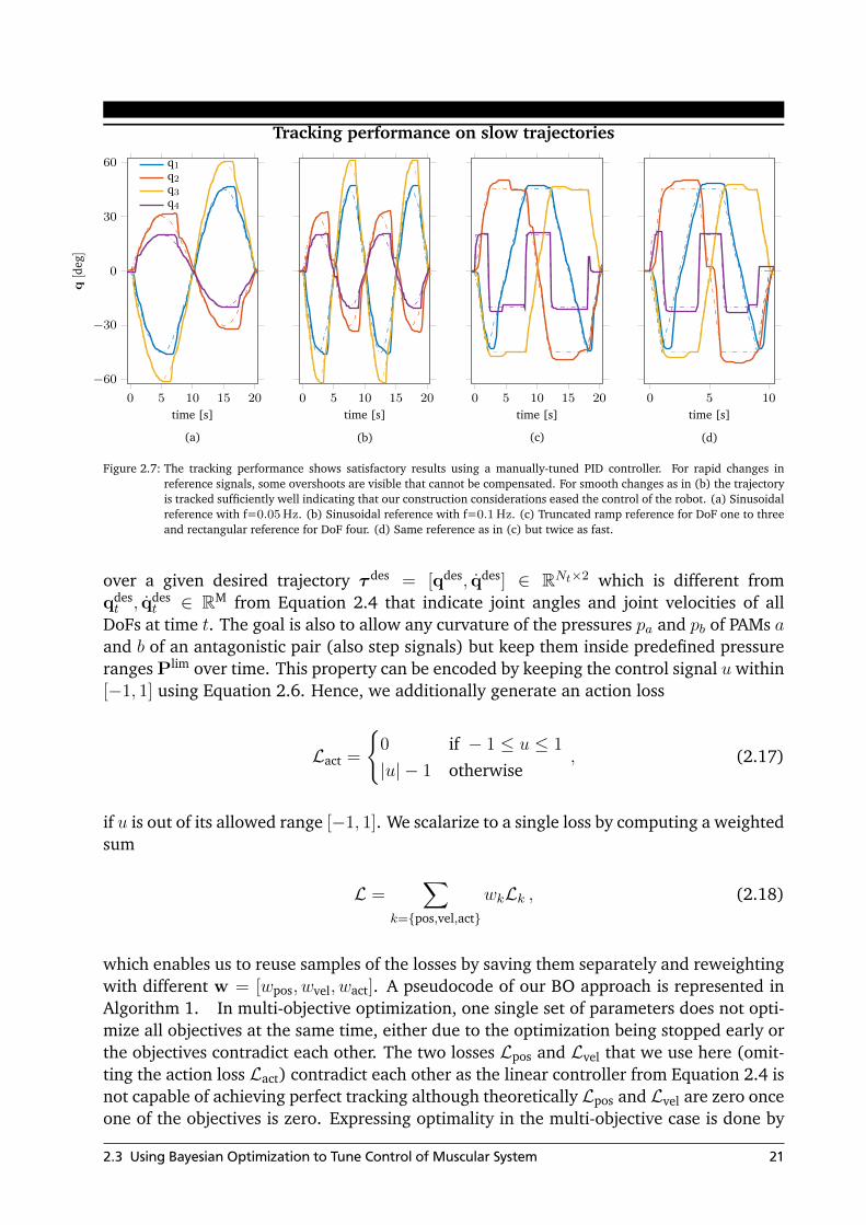
Figure 2.7: The tracking performance shows satisfactory results using a manually-tuned PID controller. For rapid changes inreference signals, some overshoots are visible that cannot be compensated. For smooth changes as in (b) the trajectoryis tracked sufficiently well indicating that our construction considerations eased the control of the robot. (a) Sinusoidalreference with f=0.05 Hz. (b) Sinusoidal reference with f=0.1 Hz. (c) Truncated ramp reference for DoF one to threeand rectangular reference for DoF four. (d) Same reference as in (c) but twice as fast.

over a given desired trajectory τ des = [qdes, qdes] ∈ RNt×2 which is different fromqdest , qdes

t ∈ RM from Equation 2.4 that indicate joint angles and joint velocities of allDoFs at time t. The goal is also to allow any curvature of the pressures pa and pb of PAMs aand b of an antagonistic pair (also step signals) but keep them inside predefined pressureranges Plim over time. This property can be encoded by keeping the control signal u within[−1, 1] using Equation 2.6. Hence, we additionally generate an action loss

Lact =

{0 if − 1 ≤ u ≤ 1

|u| − 1 otherwise, (2.17)

if u is out of its allowed range [−1, 1]. We scalarize to a single loss by computing a weightedsum

L =∑

k={pos,vel,act}

wkLk , (2.18)

which enables us to reuse samples of the losses by saving them separately and reweightingwith different w = [wpos, wvel, wact]. A pseudocode of our BO approach is represented inAlgorithm 1. In multi-objective optimization, one single set of parameters does not opti-mize all objectives at the same time, either due to the optimization being stopped early orthe objectives contradict each other. The two losses Lpos and Lvel that we use here (omit-ting the action loss Lact) contradict each other as the linear controller from Equation 2.4 isnot capable of achieving perfect tracking although theoretically Lpos and Lvel are zero onceone of the objectives is zero. Expressing optimality in the multi-objective case is done by


00.1

0.20.3

00.2

0.4

0

0.5

x1 [m]

x 2[m

]

x 3[m

]

(a)

0 0.1 0.2 0.3 0.40

5

10

time [s]x

[m/s

](b)

0 0.1 0.2 0.3 0.4−400

−200

0

200

time [s]

x[m

/s2]

(c)

0 0.1 0.2 0.3 0.4

0

500

1,000

1,500

time [s]

q[d

eg/s

]

(d)

q2q3

0 0.1 0.2 0.3 0.4−6

−4

−2

0

2

·104

time [s]

q[d

eg/s

2]

(e)

q2q3

Figure 2.8: High velocity and acceleration profiles in task and joint space. DoF 2 and 3 were actuated with the maximum pressuremoving in between the joint limits. (a) Trajectory of the end-effector in task space. (b) Velocity profile along thetrajectory in (a). Maximum value is 12m/s. (c) Acceleration profile along the trajectory in (a). The maximum valuereaches up to 200 m/s2. (d) Angular velocity profile for both swivel DoF. DoF 3 is faster as it has to accelerate lessweight than DoF 2. The maximum value of about 1500 deg/s is reached with DoF 3. (e) Angular accelerations show amaximum of approximately 28000 deg/s2


Visualization of learned hitting motion

(a) time = 1 s (b) time = 1 s . . . 3 s (c) time = 3 s . . . 4 s (d) time = 4 s . . . 5 s

Figure 2.9: Images extracted from a video showing the trajectory tracked in Figure 2.10. The images represent distinctive phasesof the learned motion: (a) zero position, (b) move to start position, (c) hitting motion and (d) move back to zeroposition.

calculating the Pareto front (PF). This set consists of points of non-dominated parameterswhere parameters θ1 dominate parameters θ2 if

θ1 � θ2

{∀ i = [1, N ] : Li(θ1) ≤ Li(θ2)

∃ j = [1, N ] : Lj(θ1) < Lj(θ2) ,(2.19)

which, in other words, means that θ1 is strictly better in at least one objective comparedto θ2 and not worse in all other objectives.

2.4 Experiments and Evaluations

Having derived our approach to tune control parameters for our developed system auto-matically, we now perform experiments to demonstrate its feasibility. First, we show thatour construction considerations make it possible to track slow trajectories with PIDs only.In the second experiment, we demonstrate high velocity and acceleration motions to un-derline the arm’s ability to be used for hitting and generate catapult-like motions whileavoiding damages at such paces. In the last experiment, both preceding experiments arecombined by learning control (PID with feedforward terms and co-contraction) directlyon the real hardware without additional safety considerations on a fast and hitting-liketrajectory.

2.4.1 Control of Slow Movements

This experiment highlights the arm’s low controlling demands by showing that adequatetracking performance is possible on slow trajectories using linear controllers only. There-fore, we track all four DoFs simultaneously for two kinds of reference signals, as canbe seen in Figure 2.7. In Figure 2.7c and Figure 2.7d a truncated triangular signal wastracked for 10 s and 20 s, respectively. The controller from Equation 2.3 has been used andthe co-contraction parameter from Equation 2.6 is p0 = 0. All graphs show that for rapidlychanging references, tracking becomes inaccurate. This deficiency is caused by the PIDsassuming a linear system while PAMs are inherently nonlinear. Additionally, for abruptcorrections, in the first moments, the change of pressure in the PAM does not affect thejoint angle in case the PAMs are not co-contracted enough [11]. For severe cases, this for-bearance is followed by a too strong correction as can be seen for DoF two in Figure 2.7a

2.4 Experiments and Evaluations 23

Tracking performance on fast trajectory after tuning with Bayesian optimization

1 2 3 4 5 6

−80

0

80

time [s]

join

tan

gle

[deg

]

qopt1

qman1

qdes1

(a) DoF 1

1 2 3 4 5 6

−70

−20

0

time [s]

qopt2

qman2

qdes2

(b) DoF 2

1 2 3 4 5 6

−60

0

60

time [s]

qopt3

qman3

qdes3

(c) DoF 3

1 2 3 4 5 6

−20

0

20

time [s]

qopt4

qman4

qdes4

(d) DoF 4

Figure 2.10: Tracking performance for all degrees of freedom after optimization using Bayesian optimization (indicated by thesubscript ’opt’) and after manual tuning by an expert on the system (indicated by the subscript ’man’). The trajectorytracked resembles an example of a fast hitting motion between t = [3 s, 4 s]. It is composed of a slow motiontowards the start position (1 s. . .3 s) followed by a fast hitting motion (3 s. . .4 s) and a motion back to the zeroposition (4 s. . .5 s) (see Figure 4.5). The manual parameters are used to track the currently not optimized DoFs inAlgorithm 1 as θman. It is apparent that tracking quality for DoFs three and four is more impaired as for DoFs oneand two due to higher friction as the cables are guided through the arm. Additionally, the PID with feedforwardcompensation assume a linear system, hence, BO optimizes towards higher gains as the system is heavily nonlinear.


and c for the middle part of the graph. This DoF drives the most mass and hence is harderto control precisely compared to the other DoFs. Sub-figures 2.7b and d show trackedsinusoidal references with 0.05 and 0.1 Hz. Here the same issues occur for rapid changesof the reference. However, for smooth changes, the reference can be followed with somesmall delay with all DoF.

2.4.2 Generation of Ballistic Movements

High accelerations are necessary to reach high velocities on a short distance to enable aversatile bouquet of possible trajectories and fast reactions. Our system can generate highvelocities and accelerations due to the strength of the PAMs used while being robust dueto the antagonistic muscle configuration. This property is critical for the exploration offast hitting motions using learning control methods. In this experiment, we show thatthe system can sustain the fastest possible motion that can be generated with our systemusing the rotational DoFs two and three. The respective minimum pressure was set toone of the PAMs of each muscle pair while the maximum pressure was assigned to theantagonist. The subsequent switching from maximum to minimum and vice versa gen-erated a fast trajectory at the end-effector, as shown in Figure 2.8a. Note that this stepset signal generates the fastest movement at the end-effector that a closed-loop controllercould have determined without instabilities. We did not find any other set signal thatmoved the arm that close to its joint limits and generated such high peak velocities andaccelerations. The task space x = [x1, x2, x3]T has been determined from the joint spacecoordinates q = [q1, q2, q3, q4]T for each data-point using the forward kinematics equationsx = T qx(q). The forward kinematics equations can be derived from Figure 2.4b. We do notconsider the orientation of the end-effector here. The resulting velocity and accelerationprofiles, depicted in Figure 2.8b and c, show at their respective maxima approximately12 m s−1 and 200 m s−2. As a comparison, the fast Barrett Wam arm used for table tennisin [36], can generate peak velocities of 3 m s−1 and peak accelerations of 20 m s−2. Theresulting angular velocities in DoF three reaches up to 1400 ° s−1 and angular accelerationof 28 000 ° s−2.

2.4.3 Bayesian Optimization of Controller Parameters

Having demonstrated that the robot arm can be controlled using simple PIDs for slow tra-jectories and that the system sustains fast hitting motions, the natural next goal is to learnto control fast trajectories (see Figure 4.5). At higher speeds, tuning control parameterslead to potentially dangerous configurations on traditional motor-driven systems that wecan partially avoid using antagonistic actuation, as discussed in Section 2.3.1. We tuneseven parameters

θi = [kPi , k

Di , k

Ii, k

posi , kvel

i , kacci , p0,i] (2.20)

for each of the four DoFs i = 1 . . . 4 (28 parameters in total) where the additional feedfor-ward components from Equation 2.4 improve control on fast trajectories.In addition to the feedback and feedforward components’ parameter, we also optimizethe co-contraction parameter p0 from Equation 2.6. Too much co-contraction increases


Similar co-contraction levels appear close to the PF in the objective space

0 10 20 30

200

400

600

Lpos

Lve

l

est. Pareto front

(a) DoF 1

2 4 6 8 10 12

150

200

250

300

Lpos

(b) DoF 2

20 40200

400

600

800

1,000

1,200

Lpos

(c) DoF 3

100 200 3000

0.5

1

1.5

·104

Lpos

0

0.2

0.4

0.6

0.8

1

p0

(d) DoF 4

Figure 2.11: Objective space that spreads the velocity Lvel and position objective Lpos from Equation 2.16 and Equation 2.15for allfour DoFs where each point represents one tracking instance of the trajectory from Figure 2.10. The color indicatesthe value of co-contraction parameter p0. Note that the figures are zoomed in to illustrate the estimated Paretofront (PF), hence, differently colored points lie outside this area. It is apparent that points with similar p0 appearclose to the estimated PF instead of being diverse. Substantially different colors are almost not present (except of forDoF three) as they lie outside the zoomed area. The dominant co-contraction range close to the PF is p0,1 = 0.9 . . . 1for DoF one (a), p0,2 = 0.5 . . . 0.7 for DoF two (b), p0,3 = 0.2 . . . 0.5 for DoF three (c) and p0,4 = 0.6 . . . 0.9 forDoF four (d).


Minimum overall objective trace

0 20 40 60 80 100 120 140 160 180 200101

102

103

104

iterations

log(L

)

DoF 1

DoF 2

DoF 3

DoF 4

Figure 2.12: Minimum overall objective trace over 200 iterations for each DoF. All DoFs start at different initial values as theparameter for the first iteration are drawn randomly. After approximately 60 iterations the performance has improvedby at least one order of magnitude. The main contributer is that our approach uses additionally potentially dangerousdata points which would break traditional motor-driven systems.

the friction within the tendon-driven system, whereas too low p0 complicates control asthe tendons are not stretched for some configurations. Hence, we aim to answer whetherthe stiffness in a joint - using the co-contraction p0 as a proxy - influences the trackingsignificantly. Optimizing 28 parameters in total renders manual tuning impossible.Figure 2.10 depicts the tracking performance that is achieved after two hours of manualtuning (qman

i ) by an expert on the system. Especially troublesome is the interdependenceof the DoFs. Tuning one DoF to a satisfactory performance often impairs the trackingof the other DoFs. Hence, we incorporate the BO tuning scheme from Algorithm 1 (de-scribed in Section 2.3.4) to tune one DoF at a time and apply either manual parametersθmani or the optimized parameters θopt

i in case they were already found to the other DoFsi. We use the position Lpos and velocity losses Lvel from Equation 2.15 and Equation 2.16respectively as performance measure. Although we also employ the action loss Lact (Equa-tion 2.17), it merely acts as a regularizer to allow all curvatures of the action signal withinthe allowed range [−1, 1] while penalizing exceeding these limits. Figure 2.10 illustratesthe tracking performance found (qopt

i ) by applying Algorithm 1 and Table 2.2 comparesthe mean squared error between the corresponding tracking performances. The algorithmconverges quickly after 200 iterations for each DoF, as shown in Figure 2.12. To the best ofour knowledge, this is the fastest tracked trajectory with a four DoF PAM-based robot (seeFigure 4.5 for an illustration of the trajectory). We think that the main advantage gainedis that our BO tuning procedure additionally learns from data points that would breaktraditional robotic systems. As a result, our approach pioneers the direct application ofBayesian optimization on a real system on a task that potentially breaks the system. Notethat the parameters we found are only valid in the vicinity of the desired trajectory wechose. The reason is that the control architecture is inherently linear and hence the sameparameters are generally valid for linear systems.

The amount of co-contraction p0 is an essential property of PAM-based systems. An in-finite set of pressures in one PAM pair leads to the same joint angle; the co-contractiondiscriminates this infinite set. Also, it correlates with the stiffness in the DoF. An interest-


ing question is whether the right choice of co-contraction improves control performance.To answer this question, we study the connection between loss and co-contraction. Fromall the points for each DoF, we calculated the estimated Pareto front (PF) using Equa-tion 2.19 and colored the data depending on the value of the co-contraction parameterp0. Figure 2.11 shows the objective space for each DoF, where one point represents onetracking instance. The figure spans the position Lpos as well as the velocity objective Lvelfrom Equation 2.15 and Equation 2.16. We left out the regularizing action objective Lact.Not all data points are visible as the figures are zoomed to illustrate the PF more clearly. Itis apparent that close to the PF, the values of p0 are similar. In particular, for DoF one, two,and four, significantly different colors do not appear in the figure at all as they lie outsidethe zoomed-in area. The absence of a whole range of co-contraction levels is a stronghint that by choosing p0 conveniently, a linear controller can better control our generallynonlinear system.

2.5 Conclusion

Generating high accelerations with robotic hardware as seen in human arm flick motionswhile maintaining safety during the learning process are desirable properties for modernrobots [4]. In this chapter, we built a lightweight arm actuated by PAMs to try to ad-dress this issue. Our robot avoids fundamental problems of previous PAM-driven arms,such as unnecessary directional change of cables and PAMs that are bent around or touchthe structure or other PAMs. We experimentally show that our system eases control bytracking a slow trajectory sufficiently while incorporating only simple and manually tunedlinear PID controllers. Execution of ballistic movements illustrates that our arm surpassesthe peak task space velocity and acceleration of a Barrett Wam arm by a factor of 4x and10x, respectively. Experiments also show that our system can sustain the large forces gen-erated by high accelerations and antagonistic actuation. This property allows machinelearning algorithms to explore in high velocity regimes without taking safety into account.To demonstrate this ability, we automatically tuned PID controllers with additional feed-forward components using BO to learn to track a fast trajectory. Predefined pressure andparameter limits were sufficient to avoid damaging the robot itself and prevent unboundedinstabilities during training. We did not find any other reported publication that trackedfaster trajectories with a comparable PAM-driven system. Data points collected duringtraining indicate that trials close to the estimated PF own similar co-contraction levels.In this manner, we empirically illustrate that the choice of the co-contraction level hasa significant influence on the performance at trajectory tracking tasks. From these re-sults follows that softly actuated robots offer robustness, which enables the applicationof powerful algorithms that, in turn, enable to perform complex tasks at a high level ofperformance. Interesting future directions are to extend the system to six DoFs to allow toreach arbitrary positions and orientations with the end-effector. This extension enables usto perform more complex tasks that require a higher number of DoFs, such as table ten-nis (requires at least five DoFs). We are also curious to learn low-level control (in musclespace), for instance, using reinforcement learning (RL), to perform more complex tasksthat involve fast motions. By allowing RL to explore in fast regimes, RL might be able tolearn well-performing policies. These policies have the chance to be less conservative as


safety wrt robot intactness is handled inherently. Another interesting direction is to un-derstand the extent to which pretrained policies in simulation can be used directly on thereal system for high-acceleration tasks. Lastly, it is intriguing to extend the research onhow to leverage the overactuation derived from the co-contraction. This inherent propertyis essential when tuning controllers for trajectory tracking, as shown in this chapter, butmight pose more challenging control demands due to increased state dimensionality, etc.

2.5 Conclusion 29

Table 2.1: A collection of pneumatic based robotic arm-like systems, listed next to the number of DoFs in joint space and the fastestand most complex tracked trajectory if known.

Year Publication # DoF Fastest and most complex trajectory tracked

2018 Driess et al. [13] 2 (5 PAMs) Reaching motions

2016 Das et al. [14] 2 Step signal to both DoFs

2014 Rezoug et al. [15] 7 Sinusoidal reference with f = 1 Hz for one DoF

2012 Hartmann et al. [16] 7 Sinusoidal reference in task space (x: f = 1 Hz, y: f = 2 Hz, z not tracked)

2012 Ikemoto et al. [17] 7 (17 PAMs) Human taught reference (similar to sinusoidal) periodic with f∼0.33 Hz

2009 Ahn and Ahn [18] 2 Triangular reference with f = 0.05 Hz

2009 Shin et al. [19] 1 (4 PAMs) Sinusoidal reference with f = 6 Hz for one DoF

2009 Van Damme et al. [20] 2 (4 PAMs) Sinusoidal reference with f = 0.33 Hz for both DoFs

2007 Festo Airic’s arm [21] 7 (30 PAMs) N/A

2006 Thanh and Ahn [22] 2 Circular with f = 0.2 Hz using both DoFs

2005 Hildebrandt et al. [23] 2 Step and sinusoidal reference with f = 0.5 Hz

2005 Tondu et al. [24] 7 N/A

2004 Boblan et al. [25] 7 in arm N/A

2000 Tondu and Lopez [26] 2 Independent sinusoidal activation of each DoF with f = 0.1 Hz

1998 Caldwell et al. [27] 7 Response of shoulder joint to 90° step reference

1995 Caldwell et al. [28] 7 Response to a square wave reference input (f = 0.2 Hz, 1 DoF)

Table 2.2: Root mean squared error (RMSE) comparison of tracking objectives for manually tuned parameters (MANUAL, θman)from Figure 2.10 and tracking with parameters found with our Bayesian optimization approach (Algorithm 1) fromFigure 2.10 (OPTIMIZED, θopt).

# DoF RMSE manual RMSE optimized

1 12.08 3.29

2 11.06 2.00

3 7.22 3.74

4 3.47 2.11


3 Control of Musculoskeletal Systemsusing Learned Dynamics Models

In the previous chapter, we built a lightweight robotic arm with eight PAMs. We illus-trated its robustness at fast movements due to the antagonistic actuation which allows toexplore dynamic tasks as required for learning control approaches. We showed that byautomatically tuning the feedforward, feedback and co-contraction terms, it is possibleto achieve precise trajectory tracking of a fast and hitting-like motion. Controlling suchmusculoskeletal systems, however, still remains a challenging task due to nonlinearities,hysteresis effects,massive actuator delay and unobservable dependencies . Despite suchdifficulties, muscular systems offer many beneficial properties to achieve human compara-ble performance in uncertain and fast-changing tasks in addition to the benefits mentionedin the previous chapter. For example, muscles are backdrivable and provide variable stiff-ness while offering high forces to reach high accelerations. In addition, the embodiedintelligence deriving from the compliance might reduce the control demands for specifictasks.In order to use these properties, it is important to address the problem of how to im-prove accurate control of musculoskeletal robots using learned models. Analytical modelsof such robots have been proposed for multiple decades. We thing that models learnedfrom data have a higher chance to exceed existing performance than an additional effortof classical modeling of musculoskeletal systems. In particular, we propose to learn prob-abilistic forward dynamics models using Gaussian processes, and, subsequently, to employthese models for control. However, Gaussian processes dynamics models cannot be set-upfor our musculoskeletal robot as for traditional motor-driven robots because of unclearstate composition etc. We hence empirically study and discuss in details how to tune theseapproaches to complex musculoskeletal robots and its specific challenges. Moreover, weshow that our model can be used to accurately control a real four DoF robot arm driven byeight pneumatic muscles for a trajectory tracking task while considering only 1-step aheadpredictions of the forward model. Key to the good tracking performance is regularizationwith variances of the Gaussian process.

3.1 Introduction

Most dynamic activities that appear straightforward for humans, such as walking, grasp-ing or ball games, are still fundamental challenges in robotics. Uncertainty, required fastreactions and necessary high accelerations – without damaging the system and environ-ment – still pose big hurdles. Despite the existence of algorithms that outperform humansin non-robotics tasks [1], the transfer to super-human performance to robots in dynamictasks has not been shown yet.

33

Using muscular robots can be a way to achieve human-level performance in robotics. Inthis work, we try to leverage antagonistic pairs of pneumatic artificial muscles (PAMs)instead of traditional motors. PAMs are the nearest replica of skeletal muscles availableas robotics hardware and share many desired properties [43]. First, PAMs are backdriv-able, thus, damages at low velocity impacts with humans, external objects and the robotitself are reduced although not completely prevented. On the other hand, changing co-contraction levels adjust the compliance in the antagonistic pair, offering flexibility if thetask requires it. Second, high accelerations, provided by PAMs, enable the robot to reachdesired states in less time and allow for fast flick-movements due to energy storage as ob-served in fast human arm movements. Third, learning dynamic tasks, e.g. table tennis, ismore feasible with antagonistic actuation as damage due to exploration at higher velocitiescan be minimized [4].Fourth, it has been shown that the demands on the control algorithm are reduced fortasks where contact with external objects is required, e.g. opening a door [50, 51]. Alsomuscular actuation assures gait stability despite of the presence of unmeasured distur-bances [52], a desirable property that might cope with uncertainties of dynamic tasks.These insights illustrate what is known as embodied intelligence and may – in combina-tion with a learning control approaches – pave the way to human-level movements.Yet, muscular robots are not widely used. Many of the issues with pneumatic musclesultimately derive from the lack of good dynamics models that generally describe therelationship between the action a taken in state s and the successor state s′. Severelynon-linear behavior, unobservable dependencies like temperature, wear-and-tear effectsand hysteresis [43] renders modeling of PAM systems considerably challenging.Another reason why muscular robots are scarcely in use is overactuation. An infinite setof air pressure combinations in an antagonistic PAM pair lead to the same joint angle butwith different compliance levels. Compliance c = δq/δFext or its inverse the stiffness krepresents the external force Fext applied to the joint required to cause a change of δq inthe joint angle. Overactuation is critical for two reasons. First, overactuation principallyrules out acquiring inverse models a = f(s, s′) of musculoskeletal systems by traditionalregression. Inverse dynamics models are only unique for traditionally actuated robots andhave to be approximated locally for over- and under-actuated systems [53]. The secondreason is, that overactuation expands the state-action space, thus, learning such dynamicsmodels requires more data or additional assumptions about the underlying mechanisms.Using forward models s′ = f(s, a), however, does not fully solve the issue despite describ-ing the true causal relationship and hence always exist. In interplay with a controller, theactions are based on predictions of the forward dynamics model.Without any additional constraints, such a controller would find potentially equally opti-mal outputs and finding optimal actions results in optimization of non-convex loss func-tions.The straightforward constraint is minimal energy, hence always choosing the minimal pres-sures that lead to the minimal control error. Another possibility is to change stiffness orcompliance according to the task, e.g., for grasping of a delicate objects. The main ideaof our approach is to pose a constraint that eases the use of a learned non-parametric andprobabilistic models. In the face of the above-mentioned difficulties of retrieving goodmodels, learning a flexible model purely from data seems to be a promising way. Recent

34 3 Control of Musculoskeletal Systems using Learned Dynamics Models

0 2 4 10

0

0.5

1

t [ 1100

s]

(a)

0 2 4 10 12

t [ 1100

s]

pdes

pqqq

(b)

Figure 3.1: System responses to a step in control signal at t = 0. All values have been normalized to be in [0, 1]. It can bee seenthat q reaches its minimum faster than q and q. (a) Unfiltered sensor values show a faster response as any filteringadds delay. The first substantial changes occurs at t = 2. (b) Filtered values reach their respective minimum slowerthan in (a). The first substantial changes occurs at t = 3, hence 1 time step later than the unfiltered signals.

successes in Gaussian process (GP) dynamic models [54, 55, 56] are especially encour-aging to follow this line of research. However, the application of nonparametric modelsin an online setting requires – among other considerations – the selection of a small setof informative training data points from a stream of highly time-correlated data stream.Hence, it is possible to deviate into unknown state-action regions, especially with time-variant systems like pneumatic muscles. In order to enable nonparametric model learningfor antagonistically actuated systems despite higher dimensionality due to overactuation,we use the uncertainty of the GP model as an additional constraint.The contribution of this chapter is twofold. First, we discuss important aspects of learningmodels for muscular systems as they are substantially different to traditional robots. Thederived key aspects are empirically compared. Second, we show how to incorporate theuncertainty of the GP dynamics model into our control framework so as to make use of theoveractuation to stay in the vicinity of the training data.

3.2 Model Learning & Control

Learning flexible and probabilistic forward dynamics models and using them for controlis a promising way to achieve better performance with muscular robots. Gaussian pro-cess (GP) regression is a non-parametric and probabilistic model that is widely used torepresent robot dynamics [53]. Here, we address how to adapt such a GP model formuscular systems and discuss the additional difficulties that arise compared to dynamicsmodeling for traditionally actuated robots. Following, we show how to use uncertaintyestimates of the GP model during control to exploit the overactuation inherent to muscu-loskeletal systems in order to generate trajectories which stay close the training data.

3.2.1 Traditional Model Learning with Gaussian Processes

Muscular robots are substantially different to motor-driven systems. After giving somebackground on forward dynamics modeling with GPs of motor-driven robots, we brieflydescribe the Hill-muscle model to illustrate our adaption of the GP model setup.

3.2 Model Learning & Control 35

Dynamics Models

Generally, the dynamics of a robot that represents the relationship between joint angles qand its derivatives q and q to the torque vector τ are modeled by differential equationsderived by applying Newtons second law and assuming rigid links

M(q)q + C(q, q)q + g(q) = τ , (3.1)

with M being the joint space inertia matrix, C represents the Coriolis and centrifugalforces and g gravitation. For traditional motor-based robots the torque τ is proportionalto the input current. Hence the relationships (q, q, τ) → q and (q, q, q) → τ representforward and inverse dynamics. The state here is clearly defined to be s = {q, q} and qcan be used as successor state s′ because the actions τ directly influence q and the stateentities can be recovered by differentiation. For muscular robots the state composition isnot obvious. The torque τi = Fi × ri depends on the combined force of all muscles actingon joint i, Fi, as well as the geometry of the joint, specifically the moment arm ri. For anantagonistic muscle pair with a radial joint, the torque reduces to

τi = (Fa − Fb)ri , (3.2)

given the forces of both muscles Fa and Fb and the angle independent radius ri.

Analytical Muscle ModelMany analytical force models for skeletal muscles exist. One of the most widely used isthe Hill muscle model, see [57] for a detailed description. It has been shown that the Hillmodel reflects the properties of PAMs to some extend [32]. The total muscle force

FM = FCE + FPEE = FSEE , (3.3)

derived from this model is based on an active contractile element FCE that depends onthe activation a and a passive parallel and serial elastic element FPEE and FSEE that bothchange with the muscle length lM . The active part of the total force

FCE = aFmaxfL(lCE)fV (vCE) , (3.4)

depends not only on the activation a but also on the force-length fL and the force-velocityfV relationship and is parameterized by the maximum isometric force Fmax. Typically, fLis bell-shaped whereas a sigmoid-like function constitutes fV . Equation 3.4 can than beused to form the dynamics of the muscle length

∂lCE∂t

= f−1V

(FSEE − FPEEaFmaxfL(lCE)

), (3.5)

that takes the activation a and lCE as parameters, resulting from the interaction of τ inEquation 3.1. Often the activation is modeled as a non-instantaneous process based on aneural excitation signal u

∂a

∂t= ca(a− u) , (3.6)

in which ca is the constant activation and deactivation rate.


0 1,000 2,000 3,000

−0.4

−0.2

0

0.2

0.4

∆q

[deg

]

(a)

950 1,000 1,050 1,100 1,150 1,2000.1

0.2

0.3

(b)

0 2,000 4,000 6,000

−4

−2

0

2

4

# training data

∆q

[deg

]

(c)

270 280 290 300 310 3200

1

2

3

4

# training data

filt(y)y

(d)

Figure 3.2: Datasets under consideration in this work depicted for illustration. All datasets were created by applying periodicpressure trajectories and recording the resulting sensor values. The target ∆q represents the difference to the nextstate and is depicted in filtered and raw sensor form. A non-causal 10th order butterworth lowpass filter was used forfiltering. (a) ’slow’ dataset. (b) Closer view of (a) illustrates that the relative angle encoders add considerable noisefor slow motions. (c) ’slow’ and ’fast’ datasets form the ’mixed’ dataset. (d) Closer view of fast part of (c). For fastermovements the noise smaller. Hence, the ’mixed’ dataset includes two types of noise. Faster movements excite higherorder dynamics components which need to be expressed by the model.


Gaussian Processes Forward Dynamics ModelsIn this chapter, we learn a probabilistic Gaussian Process [9] forward dynamics model indiscrete-time

st+1 = f(st, at) + ε , (3.7)

with s ∈ RD being the state, a ∈ RM the control action, and ε ∼ N (0,Σn) i.i.d. Gaussianmeasurement noise with a diagonal covariance noise matrix Σn. The state transfer functionf is modeled by a Gaussian process with a squared exponential kernel and automaticrelevance determination (ARD)

k(xa,xb) = σ2f exp

(−1

2(xa − xb)

TΛ−1(xa − xb)

), (3.8)

having signal variance σ2f and squared lengthscales Λ = diag(l21, . . . , l

2D+M ). The data set

D = {X,y} consist of a design matrix X ∈ RN×D+M with each row being the nth traininginput xTn = [sn, an]T and y ∈ RN the target values. Hence, one GP is established for eachelement of s′. A GP can be seen as a distribution over functions and is queried using theconditional (posterior) probability

p(f |X,y,x∗) = N (kT∗ α, k∗∗ − kT∗ Kk∗) , (3.9)

where [k∗]n = k(x∗,xn), k∗∗ = k(x∗,x∗), α = Ky and K = (K + σn)−1. The hyper-parameters σf , σn and Λ are optimized by maximizing the marginal likelihood p(y|X).The GP provides a flexible model by assuming only smoothness of the underlying functionf , depending on the choice of the covariance function. On the other hand, a this non-parametric training data set is required to make predictions which needs to be kept andthe prediction time complexity rises cubical with its size N O(N3). Many approximationsschemes exist [58, 59] that are term to future work but are not used here as they rely onapproximations.

3.2.2 Model Adaptations to Muscular Systems

Many properties of pneumatic muscular systems render modeling difficult. We mentionsome of this issues from which we subsequently derive adaptations to the GP forwarddynamics model.

Modeling Issues

Modeling of PAMs is still a key problem for control [43]. The reason for this is that analyt-ical models derived from physics, including the Hill muscle model from Equation 3.4, donot sufficiently describe aspects of real PAMs. Unobserved influences like volume change ofthe muscle while moving, tip effects and temperature as well as hysteresis, nonlinearitiesrequire the model to be extraordinary flexible. Additionally, some parameters in analyticalmuscle models are kept constant for simplicity and avoiding high computational load.


Another important issue with pneumatics is actuator delay. In every system a short timepasses between applying control until a reaction is sensed. The time in between sumsup all delays in the control loop. For instance, a magnetic field that has to increase in amotor or – as in our case – valves have to open and air pressure has to rise in PAMs. ForPAM-actuated robots, the sequence of actuation

pdes → uvalve → air flow→ p→ τ → q→ q→ q ,

contains more sources of delay compared to motor-driven systems, e.g., mechanical open-ing and closing of the valve and the generation of air pressure in the muscles. This processis further delayed by the compressibility of air. Figure 3.1 shows an experiment where thejoint angles q, velocities q and accelerations q are recorded in response to a step in desiredpressure signal pdes for unfiltered and filtered case. Unfiltered entities respond faster tothe excitation but inhere more noise, especially higher time-derivatives like joint veloci-ties q and accelerations q because they need to be estimated. Strong noise complicatesmodeling with GPs as only output noise is assumed.

State Composition

Another consequence from severe actuator delay is that the successor state s′ is dependenton the current state s and action a as well as previous states and actions. When formulatinga control task as a Markov decision process (MDP, [60]), the forward dynamics or transitionfunction is, however, required to establish a relationship where s′ depends only on s anda. In an MDP the state has to bear the Markov property

p(st|a1:t, s0:t−1) = p(st|at, st−1). (3.10)

This requirement is often violated when the dependence on the past is weak and lead to amodel that is sufficiently good. On real systems, dependencies often remain unmeasureddue to the lack of sensors or tedious measurement procedures. Estimating the temperaturein PAMs is an example which influences the behavior of the rubber material as well as thecompressibility of the air. Ideally, the temperature is measured over the complete lengthof the muscle, on the material itself and the air inside the muscle. This is not feasible andour system is not equipped with temperature sensor. The same line of thinking is true forstiction and friction effects as well as slack of the cables. Nonetheless, the information ofsuch unobserved effects is captured in the transition (st, at) → st+1 as different successorstates will be reached when applying the same action in the same state at different times.Such a problem is described as a partially observable MDP (POMDP).A possible solution to this problem is to approximate this POMDP with a K-th order MDPby concatenating the previous states and actions into an augmented state

saugt = [st, st−1, . . . , st−k, at, at−1, . . . , at−k]. (3.11)

an idea closely related to the NARX concept [61].


State Elements based on Analytical ModelsThe components of the state can be obtained by the rigid body dynamics Equation 3.1and the analytical model Equations 3.6 and (3.5). Hence, q, q as well as l, l, p and pshould be part of the state. Here l denotes the vector of muscle lengths and p the vectorof current PAM air pressures. Incorporating the pressures p into the state also helps toresolve hysteresis effects because rising and falling curves can be discriminated accordingto pt ≤ pdes

t . The order of the system determines how many time-derivatives need to beadded to the state. While it is clear from rigid body dynamics Equation 3.1 that the robotarm is a second order system, it is not clear what the order of the PAMs as analyticalmodels for PAMs do are not as well established as the rigid body dynamics equations fortraditional robots. For instance, [57] indicates that the activation from Equation 3.6 shouldpossibly be modeled as a second order system but don’t take the higher order into accountto reduce computational load. In addition, for slower movements higher order derivativesmight not play such an essential role in the model prediction and can be held out from thestate to avoid higher input dimensionality of the GP. For this reason, we test slow and fasttrajectory data sets in the experiments Section 2.4 and check how performance is influencewith the orders of the systems.

Estimated State ElementsAnother issue with time derivatives is that they are not sensed directly but have to beestimated. A common way is to use finite differences mt = (mt+1 − mt−1)/2∆t where∆t is the sampling period and mt a measurement. However, the noise on mt would inthis case multiply. A GP only assumes output noise and would experience major compli-cations. Unfortunately, from our experience, the delay introduced by filtering the sensorvalues online on the real robot, even with a second order butterworth lowpass filter, sub-stantially impairs control performance. We, hence, test how adding previous joint anglesqt:t−h and pressures pt:t−o instead of their respective time-derivatives alter the predictionperformance without filtering the input training data.A similar transformation as finite difference is required to attain the lengths of the cables.The lengths of the muscles are la,b = l0 ± (q/2π)r where l0 is the muscle length for q =0 deg assuming a radial joint with fixed radius r and always tensioned cables. Withouta question, the information about the lengths of the PAMs are encoded into the jointangle. An interesting question is whether the GP is able to recover such transformationsin addition to unobserved dependencies like elongation and slack of the cables. Based onthe previous discussion, we propose to test following state compositions

snoisyt = [qt, qt,pt, pt] , (3.12)

spaddedt = [qt:t−h,pt:t−o] , (3.13)

sactiont = [sx

t ,pdest:t−h] , (3.14)

where sxt is a placeholder for either snoisy

t or spaddedt . The state compositions are empirically

tested in Section 3.3.


mean(NRMSE)

0 200 400 600 800 1,0000

0.5

1

1.5

2·10−3

slow

data

set

(a)

0 200 400 600 800 1,0000

0.5

1

1.5

2·10−3

fast

data

set

(b)

0 200 400 600 800 1,0000

0.5

1

1.5

2·10−3

# training data points

mix

edda

tase

t kmeansequirandomfilt(kmeans)filt(equi)filt(random)

(c)

Figure 3.3: The influence of random, k-means and equidistant training data selections model is illustrated with increasing size oftraining data set on the (a) ’slow’, (b) ’fast’ and (c) ’mixed’ dataset. Experiments have been performed five times andthe mean result is depicted. The ’fast’ dataset is composed of similar periodic curves and hence needs the least numberof data. In case the NRMSE is calculated against unfiltered test targets, the NRMSE tends to rise for more provideddata points because the prediction of the GP becomes smoother as the noise modeling improves.


Model Validation

According to [62] a model can only be good enough to fulfill its purpose. [63] coinsthis aspect purposiveness. The process of disentangling the contribution of the modeland the controller to the performance is quite involved. Hence, often long-term predic-tions [54, 55] are analyzed. This procedure involves a previously collected data sequenceconsisting of a state [st]

Tt=0 and a corresponding action trajectory [a0]T−1

t=1 . Starting with theinitial input x0 = [s0, a0] to the GP, the prediction of next state is fed together with the nextaction as input for the next time step. This iterative procedure is being continued until thepredicted state deviates too much from the known state trajectory, e.g. ||sdes − sH ||2 > ε.The horizon H represents then how well the roll-outs can be simulated and is importantfor instance for model predictive control type of control frameworks. For muscular sys-tems, the state requires to contain the pressures inside the PAMs. Long-term predictionsare then always corrupted by the quality of the pressure model that, in return, is not pre-defined by the desired trajectory. PAM pressures play a role only when stiffness shouldbe modulated along with the position trajectory, which is not focus of this work. For thisreason, we decide to resemble to one-step-ahead predictions and only predict entities that

slow fast mixed

s(1)t = [qt]

2.6e− 04± 1.1e− 04 1.3e− 04± 2.2e− 06 4.8e− 04± 2.7e− 04

2.6e− 04± 3.6e− 05 1.3e− 04± 1.1e− 05 4.8e− 04± 3.5e− 04

2.0e− 04± 0.0e+ 00 1.3e− 04± 0.0e+ 00 3.6e− 04± 0.0e+ 00

s(2)t = [qt, qt−1, qt−2]

2.8e− 04± 3.7e− 05 1.3e− 04± 6.5e− 06 4.6e− 04± 3.0e− 04

2.0e− 04± 1.3e− 05 1.3e− 04± 3.7e− 06 3.1e− 04± 1.2e− 04

2.9e− 04± 0.0e+ 00 1.3e− 04± 0.0e+ 00 3.1e− 04± 0.0e+ 00

s(3)t = [qt, qt−1, qt−2, pat , p

bt ]

2.8e− 04± 9.0e− 05 1.3e− 04± 2.2e− 06 3.0e− 04± 6.9e− 05

2.6e− 04± 4.4e− 05 1.3e− 04± 3.4e− 06 2.8e− 04± 8.3e− 05

2.9e− 04± 0.0e+ 00 1.3e− 04± 0.0e+ 00 2.7e− 04± 0.0e+ 00

s(4)t = [qt, qt−1, qt−2, pat , p

bt , p

a,dest−1 , p

b,dest−1 ]

2.8e− 04± 6.4e− 05 1.3e− 04± 2.6e− 06 1.7e− 04± 9.0e− 05

2.3e− 04± 3.4e− 05 1.3e− 04± 5.3e− 06 9.9e− 05± 2.7e− 05

2.9e− 04± 0.0e+ 00 1.3e− 04± 0.0e+ 00 2.6e− 04± 0.0e+ 00

s(5)t = [qt, qt, pat , p

bt ]

3.4e− 04± 9.0e− 05 1.3e− 04± 1.3e− 05 4.3e− 04± 1.3e− 04

3.0e− 04± 3.6e− 05 1.3e− 04± 5.3e− 06 2.7e− 04± 1.0e− 04

3.2e− 04± 0.0e+ 00 1.3e− 04± 0.0e+ 00 3.1e− 04± 0.0e+ 00

Table 3.1: Normalized root mean squared error from Equation 3.15 calculated for the prediction of each model with different statecompositions (rows) against filtered target values from the datasets (columns) depicted in Fig. 3.2. Experiments havebeen performed five times under same conditions illustrated by the mean NRMSE and one standard deviation. 100 datapoints have been selected to the training set by random, k-means and equidistant selection. Equidistant selection isdeterministic and thus has always zero standard deviation. The best performance on the ’slow’ dataset is achieved withs(2)t and k-means selection. More complex state representations achieve worse performance. It is clearly visible that for

the ’fast’ dataset 100 training data points contain enough information and hence is independent of state composition aswell as data selection type. This confirms that with enough data the Gaussian Process design choices are less importantbut evaluation is computationally more expensive. The ’mixed’ dataset is harder to model as it is composed of differentnoise levels in addition to different speeds which require modeling of higher dynamics components. Best performanceis achieved with more complex state representations, s(4)t , as well as k-means selection that is capable to select moredistinctive data points compared to the other selection types.


are essential to calculate a control error. Many criterion exist to measure model goodnessof one step ahead predictions, see [63] for a detailed description. Here, we employ thenormalized root mean squared error

NRMSE =

√√√√∑Ni=2(f (k)(si−1, ai−1)− s(k)

i )

N(s(k)max − s(k)

min), (3.15)

where f (k) is the k-th element of the prediction and k ∈ [1, D], s(k)max and s(k)

min the maximaland minimal value of the state component k in the dataset comprising N data points.The predictions can be test either against the filtered or raw targets from the data set.The filtering of the target signal can be done with a non-causal filter, e.g. zero-phasebutterworth lowpass filter which does not add additional delay. Filtered outputs have thebenefit to be closer to the latent true data as can be seen in Figure 3.2 (b). We test bothcases in Section 3.3.

Filtering Training Outputs

We resort to filter the training outputs although a GP in principle handles output noise.However, we found state dependent noise in our training data set which requires het-eroscedastic noise treatment. Figure 3.2 (b) and (d) illustrate that the unfiltered graphchanges more randomly for the slow data set than for the fast data set. Heteroscedas-tic data sets often occur in real applications. Unfortunately, only homoscedastic GPs areanalytically tractable rather than a heteroscedastic GP whose inference is based on ap-proximations and training is computationally more demanding. By filtering the trainingtargets, different noise levels of the data set can be balanced to some extend.Using approaches to handle input noise for GPs [64, 65] is a valid alternative and is subjectto future work. In this work, we aim at highlighting problems and give basic answers.Thus, we try to avoid all approximations as quantifying where approximations influencethe result is hard to answer.

Subset Selection

Robots generate a lot of correlated data at high frequencies. Keeping all this data in thetraining data set for non-parametric data is not possible. Hence, the data need to be furthersubsampled. We do not incorporate approximations to the GP in order to realize biggertraining data sets, e.g. with pseudo inputs [58] for reasons stated above.Hence, we pick a subset of data from the complete data set instead. As a baseline weincorporate random subsampling which is equivalent to guessing. Every approach shouldimprove over random guessing. The default choice is often equidistant subsampling whereN data points are picked from the data set that are equally far apart. If, however, theresulting sampling frequency is less than twice the maximum frequency of the time series,some aspects of the signal cannot be captured according to the Nyquist-Shannon samplingtheorem. On the other hand, areas where little change happens could be sampled toooften. As an alternative, we use k-means algorithm to find N clusters among the complete


data set and pick the data point that are closest to each clusters. Thus, such data points areselected so as to maximize the difference among the training set according to the Euclideandistance.

3.2.3 Gradient-based Control

The control goal is to track a desired trajectory {sdest }Tt=1 with a control trajectory {at}Tt=1

with minimal deviation. A simple way to express this desire is to define the squared error

e2t = ||(sdes

t − st)||2Q , (3.16)

for each time step t. The mean of the forward dynamics model f from Equation 3.7 can beincorporated for the prediction of e2

t+1 in the next time step

e2t+1 = (sdes

t+1 − st+1)TQ(sdest+1 − st+1)

→ e2t+1(at) = (sdes

t+1 − f(st, at))TQ(sdes

t+1 − f(st, at)). (3.17)

The controls in each time step t can than be extracted using

at = argmina

e2t+1(a) . (3.18)

The main idea of our control framework is to make use of the full posterior distributionthat is given by our probabilistic forward model. Thus, we optimize for the expected valueof the loss, similar to [66]. In this case Equation 3.16 becomes

E[e2t+1(a)] = sdes

t+1

TQsdes

t+1 − 2sdest+1

TQE[f ] + E[fTQf ]

= sdest+1

TQsdes

t+1 − 2sdest+1

TQf + fTQf + tr(QΣ)

= e2t+1(a) + tr(QΣ(a)) (3.19)

with [Σ]i,j = cov(fi, fj) being the covariance of each GP in the forward model vectorf and diag(Σ) = σ2. Equation 3.19 can be interpreted as the sum of the mean of thesquared error from Equation 3.17 and regularized by the variances of each element of theforward model vector f weighted by the diagonal elements of Q. This regularization posesa constraint to the overactuation of antagonistic actuation. Hence, by using this controlframework, the controls are chosen such that the the successor state is near to the trainingdata set.

3.3 Setup, Experiments and Evaluations

The goal of this chapter is to illustrate how to set up a GP dynamics model and use itsubsequently for control of a muscular system. We first introduce the PAM-driven robotarm used to validate our approach. Afterwards, we address the key concepts discussedin section 3.2 with empirical experiments. For the experiments we use the slow, fast andmixed data sets from Figure 3.2 which all have the same size. The slow data set challenges


0 5 10

−30

0

30[d

eg]

qdesq

(a)

0 5 10−5

−1

1

5

[deg

]

e

(b)

Figure 3.4: Tracking experiment. The controller manages to keep the system in the vicinity of the training data. Also, the controllerdeals well with hard changes in directions of the desired trajectory and stays apart from that regions within an errorbound of ±1 deg.

the model to accurately distinguish noise from signal. As the relative angle encoders of ourmuscle based robot have a resolution of 0.036◦, relatively high quantization noise corruptsthe signal as can be seen in Figure 3.2 (b) due to quantization. The fast data set consistof rapidly repeating oscillating movement. Thus, more data represents the same curve buthigher order dynamics components are excited. The challenge of the mixed data set is itsheteroscedastic noise that often occurs in real data sets. We always predict the differenceto the next joint angle ∆q. Lastly, a tracking task is performed to show that the resultingGP forward model is useful for control.

3.3.1 Experimental Setup: Pneumatic Muscle Robot

We use the PAM-actuated robot arm from [4, 67] which is shown in Figure 2.1. Its keyfeatures are a) its lightweight structure with only 700g moving masses, b) powerful PAMsthat can lift up to 1.2kN each and generate angular accelerations of up to 28k deg/s2 andc) its design that aims to reduce difficulties for control, e.g., minimal bending of cablesetc.. This four DoF robot arm has eight PAMs in total, each two actuating one DoF asan antagonistic pair. Each PAM is equipped with an air pressure sensor and each jointangle is read by an incremental encoder. The pressure in each muscle is changed via Festoproportional valves that regulate the airflow according to the input voltage. All signalsare fed into a NI FPGA card that has in turn a C/C++ API for an interface to the mainC++ code. Low level PID controller regulate the desired pressures sent from the C++program within the FPGA. The desired pressures are bounded in the FPGA. In this manner,erroneous signals will not be executed on the real system.

3.3.2 Subset Selection and Model Validation

In this experiment we test how the prediction performance changes with the number oftrainings data points as well as subset of data selection strategy. Figure 3.3 shows thisexperiments for the (a) slow, (b) fast and (c) mixed data sets.One can observe that in all graphs the mean of the NRMSE decreases when tested againstthe filtered test targets. When tested against unfiltered test outputs the NRMSE fails at

3.3 Setup, Experiments and Evaluations 45

capturing that the model improves with more data and hence is ruled out as a qualitymeasure of 1-step ahead predictions.Another observation is that the fast data set can be learned with less training data as lessinformation is contained.In (c) one can observe that unfortunate equidistant subsampling can lead to bad perfor-mance.

3.3.3 Evaluation of State Composition

Figure 3.2 Table 3.1 comprises an experiment where the proposed states and subsamplingtypes from Section 3.2 are tested on the three different data sets from Figure 3.2. Theaverage prediction performance with 100 data points is pointed out together with onestandard deviation calculated from five identical experiments for each setting. For theslow data set s

(2)t with k-means subsampling leads to best performance. Interestingly,

more complex states perform worse. The reason is, that for states with higher dimensionsmore training data is required to fit the model well. Apparently, for simple trajectories asimple state is sufficient.The fast data set comprises less information compared to the slow data set into more datapoints. Thus, 100 data points are enough for all states to learn to model well.The mixed dataset is contains heteroscedastic noise and different curvatures and hence isthe most complex compared to the low and fast data set. s

(4)t with k-means subsampling

outperforms by far all other settings. k-means subsampling assures that the most differentdata points are picked into the training data set. In this manner, the flexibility introducedby state s

(4)t has a better chance to be utilized.

In general, for rich datasets, a more state should be chosen that enables the model tocapture all facets of the underlying data. For simpler datasets the focus can be on thecomputational load. A smaller state representation can be used in order to speed upcomputation.

3.3.4 Evaluation of Control Performance

We validate our control approach with a model that 1) filters training outputs, 2) usesk-means clustering to select training data and 3) uses s(4)

t from table 3.1 as state. The dataset is generated by utilizing a PID controller whose performance should be surpassed. Inthis way we create data that is near to the desired trajectory. The desired trajectory con-tains edges to show how the controller performs at sudden changes which are especiallychallenging. Fig. 3.4 shows the tracking experiment. The control performance stays mostof the time within a control error bound of ±1 deg. After the quick changes in reference,the controller manages to return to the desired trajectory quickly.

3.4 Conclusion

Modeling the dynamics of musculoskeletal robots with flexible Gaussian processes is apromising research direction. In this chapter, we identified key problems of using GPs to


replicate the dynamics of muscular systems and proposed appropriate solutions. Subse-quently we used this probabilistic model for control.The contribution of this chapter is twofold: First, we discuss and empirically evaluate howto set up and test a Gaussian process forward dynamics model for muscular systems. Weconsider different state compositions and subsampling types, debate where filtering makessense and how to evaluate goodness of our model. Subsequently, we tested our hypotheseson data sets with distinct properties. Second, we show that by using a probabilistic modelthe overactuation inherent to muscular systems can be resolved while enabling flexiblenon-parametric models to model the dynamics for such complex systems. We leveraged theuncertainty of the GP to set an additional constraint in the control framework that keepsthe system near its training data. The control framework developed in this chapter canbe used to tackle the problem of learning fast hitting movements by tracking trajectoriesoptimized through planning algorithms [68, 69].On the path of illuminating the connection between learning and muscular systems, thiswork posed an example to the application of Gaussian processes to dynamics modelingof muscular systems. Interesting future directions involve approaches that perform multi-step ahead predictions to improve accurate control further. Including dynamic redundancyresolution, as proposed in this chapter, to multi-step ahead prediction models might enablebetter models and hence improved control.Another interesting aspect to extend is to automatically retrieve a Markovian state compo-sition. A possible way would be to use variational autoencoders and develop regularizationterms that act on the latent space to This approach is similar to the concept of robotics pri-ors [70].The classical approach to table tennis – consisting of a planning stage optimizing a targettrajectory and a controller tracking this trajectory – includes the assumptions that thegenerated trajectory is somewhat optimal and that the controller is capable of trackingthe trajectory sufficiently well. This are effectively priors on the solution of the task. Anintriguing alternative could be to use RL and formulate the table tennis task exclusively inthe reward function without taking robot safety into account.

3.4 Conclusion 47

4 Learning to Play Table Tennis FromScratch using Muscular Robots

In the previous chapter, we learned a GP forward dynamics model of the muscular robotand used it to perform a trajectory tracking task. We regularized the control with theuncertainty estimates given by the GP model to resolve the dynamic redundancy whilekeeping the system close to its previously seen training data. In order to play table tennisusing the approach from chapter 2, a trajectory planner is required and the dynamicsmodel would have to predict well in large spaces of states and actions. The prediction timecomplexity of non-parametric GPs, however, increases linearly with the number of trainingdata points. Hence, tracking fast motions that change substantially remains unsolved. Inaddition, planning fast motions in the presence of uncertainties arising from difficult balland robot state estimation is a challenging task.

The task of table tennis can be formulated in a simple manner: the racket needs to hitan incoming ball and the returned ball needs to land on the opponent’s side of the table.An alternative approach to the one in Chapter 2, hence, is to define the task purely in areward function and use Reinforcement Learning to get a policy that performs the tabletennis task. Especially, model-free Reinforcement Learning (RL) is a compelling approachto learn complex continuous control tasks. Robot table tennis is an example of a suchdifficult task. It requires control of fast movements and precise timing. RL could helplearning to execute such fast motions from experience. However, to reach a high levelof fidelity, model-free RL requires to freely explore and fail in a safe manner for millionsof time steps in high velocity areas of the state space. Learning a dynamic tasks directlyon real robots, might push the robot to areas of the task space that bring the operationalconditions of the system in jeopardy.

The key idea of this chapter is twofold: We propose to leverage the robustness of soft robotsto run RL safely on a real robot table tennis task while RL, in turn, learns this complex taskdirectly on real hardware and overcomes the inherent control difficulties of soft robots. Inparticular, we show that it is possible to learn to return and smash table tennis balls to adesired landing point using a robot arm driven by pneumatic artificial muscles (PAMs) withmodel-free RL. Our contribution is to illustrate that, using PAM-driven robots, RL can learntable tennis like in simulation, meaning 1) without additional safety considerations 2)while maximizing the speed of the returned balls 3) using a randomly initialized stochasticpolicy 4) that acts directly on the low level controls of the real system and 5) trains forthousands of trials from scratch. We also suggest a practical semi sim and real training totrain this task without supervision. To the best of our knowledge, this work pioneers thesuccessful applications of PAM-driven robots to table tennis.

49

4.1 Introduction

Reinforcement Learning (RL) achieves great performance at ambitious tasks such as thecomplex game of Go [71], full body locomotion tasks in simulation [72] or difficult con-tinuous control tasks such as robot manipulation [73, 74] to name just a few. All of thesehard to solve tasks are either realized in simulation environments or the real robot task isengineered in a way that the RL agent can act like in simulation. In simulated continuouscontrol tasks the agent is allowed to bump into objects, collide with itself and the actionscan act on low level controls (such as torques or activations to muscles) while being sam-pled from a stochastic policy. The policy can be step-based, in contrast to episode-basedpolicies, which permits the agent to react in every time step to changes in state rather thanexecuting an open loop motion. In this manner, the agent freely explores and learns fromfailures while interacting for millions of time steps with the environment.Current real world problems to which RL is applied are constraint to merely slow motionssuch as in manipulation. For such tasks, simple engineered checks assure robot safety.

Figure 4.1: Our setup consists of a four DoF robot arm actuatedby pneumatic muscles and a ballgun that shootsballs towards the robot arm. The robot is supposedto return the ball to a desired landing point on thetable. The Cartesian positions of the ball are mea-sured by a color-based camera detection system.

This checks detect for instance 1) collisionswith objects (usually based on heuristics)and the robot itself, 2) limit joint acceler-ations and velocities, 3) stop the robot be-fore it is reaching its joint limits and 4) filternoisy actions generated by stochastic poli-cies [75, 73]. Also, the RL community in-creasingly recognizes the safety of the robotto be essential if RL should be reliably em-ployed on real robots [76, 77].For dynamic tasks like robot table tennisthis safety checks are disadvantageous fortwo reasons: 1) empirically finding parame-ters for the safety heuristics is substantiallyharder at faster motions and 2) the safetychecks heavily limit the capabilities of robotsas they are conservatively chosen in orderto reliably avoid damage to the real system.Cautious checks are fine for slow motions asthey suffice, e.g. for grasping and lifting anobject, but for a task like table tennis it is es-sential to exert explosive movements. Imag-ine that an incoming ball is supposed to behit at a point in space which is far away fromthe current racket position. In such situation,the agent needs to accelerate the racket rapidly in order to gain momentum and reach thehitting point in time. Thus, the amount of accelerations that the robot is capable of gener-ating is proportional to the upper bound on the dexterity it can reach in table tennis.To this point, it is challenging to not limit the performance of dynamic real robotic taskstoo much by safety check and let the agent explore fast motions freely. For this reason,

50 4 Learning to Play Table Tennis From Scratch using Muscular Robots

learning approaches to robot table tennis using anthropomorphic human arm sized sys-tems usually employ techniques such as imitation learning [69], choosing or optimizingfrom safe demonstrations [78, 68, 37], minimizing acceleration for optimized trajecto-ries [79], distributing torques over all degrees of freedom (DoF) [80] as well as cautiouslearning control approaches [81].

In [4, 67] it has been shown that systems actuated by pneumatic artificial muscles (PAM)are suitable to execute explosive hitting motions safely. By adjusting the pressure rangefor each PAM, a fast motion generated by the high forces of the PAMs can be deceleratedbefore a DoF exceeds its allowed joint angle range. In addition, PAM-driven robots areinherently backdrivable which makes them especially robust. However, such actuatorsare substantial harder to control than traditional motor-driven systems [43, 11]. For thisreason, PAM-driven systems are predominantly used as a testbed for control approaches.

In this chapter we show that soft actuation enables RL to be safely applicable to a dynamictask directly on real hardware and, vice versa, RL helps to overcome the difficulties of adynamic task as well as the control issues of soft robots. In particular, we show that, byusing the robot actuated by pneumatic artificial muscles (PAM) from [4, 67], we can learnto return and even smash table tennis balls using RL from scratch. Rather than avoidingfast motions, we favor highly accelerated strikes by maximizing the velocity of the returnedball where robot safety is handled inherently by the hardware. In addition, we 1) applynoisy actions sampled from a Gaussian multi layer perceptron (MLP) policy directly on thelow level controls (desired pressures), 2) while running the RL algorithm for millions oftime steps, 3) randomly initialize the policy at start and 4) introduce a hybrid sim andreal training procedure to circumvent practical issues of long duration training such ascollecting, removing and supplying table tennis balls from and to the system. Using thistraining procedure, we learn to return and smash balls without using real balls duringtraining. By enabling RL to act on the real system in the same way as in simulation, weenable to leverage the benefits of such complex systems, despite the control issues, to bethe first to learn this challenging task of playing table tennis with muscular robots.

In Section 4.2 we introduce the reward functions that have been incorporated to learn toreturn and smash as well as the hybrid sim and real training procedure. The return andsmash experiment are described in detail in Section 4.3. We summarize the contributionsand discuss this chapter in Section 4.4.

4.2 Training of Muscular Robot Table Tennis

The symbiosis of learning dynamic tasks and muscular robots allows the RL algorithm toact in the same way as in simulation while RL helps to overcome the inherent controldifficulties PAM-driven systems and leverage its beneficial properties for the task. In thissection, we introduce the return and smash table tennis task and illustrate the details ofthis symbiosis. We further introduce dense reward functions that formulate the intentionto return an incoming ball to a target location on the table and to maximize its velocity atimpact.

4.2 Training of Muscular Robot Table Tennis 51

Variability in Recorded Ball Trajectories

0 0.5 10.8

1

1.2

1.4

t [s]

x[m

]

samplesmeanstd dev

(a)

0 0.5 1

−0.5

0

0.5

t [s]

z[m

]

(b)

0 0.5 12

3

4

5

t [s]

|b|[

m/s]

(c)

020.8

1

1.2

1.4

y [m]

x[m

]

table y limits

(d)

02

−0.5

0

0.5

y [m]

z[m

]

(e)

022

3

4

5

y [m]

|b|[

m/s]

(f)

Figure 4.2: Variability of the recorded ball trajectory dataset Drec. Table tennis balls have been launched by a ball launcher withfixed settings towards the robot. Recording was done via a color-based camera vision system [82]. Variability isquantified by the sample mean and sample variance with respect to time a) to c) and along the long side of the table (ycoordinate) d) to f). The shorter edge of the table is aligned with the x coordinate and z is linked to the normal ofthe table plane. Although the settings of the ball launcher are constant, the ball varies substantially: 1) variabilityincreases over the duration of the trajectory, especially after the bounce, 2) the first bounce on the table (incomingball) varies around 50 cm along y-coordinate which can be seen from subfigure e). 3) the agent has to handle deviationof around 40 cm along the x-axis and ∼50 cm along the z-axis when the ball is in reach for the hit. 4) the variabilitywith respect to time and the y-axis increases over time which means that the agent cannot simply learn to start the hitafter a particular fixed duration. Additionally, the agent needs to learn to adjust the amount of energy it transfers toeach individual ball as the ball velocity also varies between at the end of the table.


4.2.1 Muscular Robot Table Tennis Task Setup

The table tennis task consists of returning an incoming ball with the racket attached to therobot arm to a desired landing point on the table bdes ∈ R2. We denote the ball trajectoryτ b = [sb

t ]Tt=0 consisting of a series of ball states sb

t = [bt, bt] that themselves contain thecurrent ball position bt ∈ R3 and velocity bt ∈ R3. In a successful stroke, the robot hitsthe ball at time th and position bh such that the ball lands on the table plane at positionbland at time tland. The ball crosses the plane aligned with the net on the incoming andoutgoing ball trajectory at position bnin ∈ R2 at time tnin and bnout ∈ R2 at time tnout if therobot successfully returns the ball.Table tennis falls into the general class of dynamic tasks such as baseball [83], tennis orhockey [84]. Dynamic tasks represent a class of problems that are relatively easy to solvefor humans but hard for robots. The features of dynamic tasks are 1) quick reaction timesas some moving object has to be touched or hit in time, 2) precise motions because theobject is supposed to arrive in some goal state (e.g. desired landing position on the table)and 3) fast and highly accelerated motions. The latter point is important for two reasons:First, a successful strategy can incorporate a fast strike like in a table tennis smash. Second,highly accelerated motions are required in case the desired hitting position of the ball bh

is far away from the current racket position. For this reason, the maximum accelerationthe robot system is capable of generating represents the upper limit to the dexterity theagent can develop at such tasks. This class of problems can be seen in contrast to robotmanipulation where the task itself is richer than a dynamic task in the sense that the objectsand setting can vary largely. For this set of tasks, however, slow motions are sufficient.Particularly useful for dynamic tasks are robots actuated by pneumatic artificial mus-cles (PAM). This actuators contract if the air pressure inside increases, hence at leasttwo PAMs act antagonistically on one degree of freedom (DOF) as a single PAM canonly pull and not push. In this chapter, we leverage the PAM-driven robot arm devel-oped in [4, 67] which has four DoFs actuated by eight PAMs. Such robots are capableof generating high accelerations due to a high power-to-weight ratio. At the same time,allowed pressures ranges can be adjusted such that joint limits are not reached despite fastmotions. We use this property in Section 4.3.1 and Section 4.3.2 to let the RL agent freelyexplore fast motions without further safety considerations. Another benefit of PAM-drivensystems is the inherent robustness due to passive compliance. This property helps reduc-ing damage at impact due to shock absorption [85] as well as adjusting stiffness due toco-contraction of PAMs in an antagonistic pair. In this chapter, we leverage the robustnessto apply stochastic policies directly on the desired pressures which are the low level actionsin this system (see Figure 4.4).This numerous beneficial properties come at the cost of control difficulties. PAMs 1) arehighly non-linear systems that 2) change their dynamics with temperature as well as wearand 3) are prone to hysteresis effects. Thus, modeling such systems for better control ischallenging [43, 11]. For this reason, predominately used as testbed for control algorithmsrather than utilizing the advantages of this actuators. In this work, we show that it is pos-sible to satisfy the precision demands of the table tennis task despite the control difficultiesof PAM-driven systems by using RL (see Section 4.3.1 and Section 4.3.2).


4.2.2 Dense Reward Functions For Returning and Smashing

We formulate the learning problem as an episodic Markov Decision Process (MDP)

M = (S,A, r,P , p0, γ) (4.1)

where S is the state space, A is the action space, r : S × A 7→ R is the immediatereward function, P : S × A 7→ S is the transition probability or dynamics, p0 is theinitial state distribution and γ ∈ [0, 1] the discount factor. The goal in RL is to find apolicy π : S 7→ A that maximizes the expected return J = Eτ

∑Tt=0 γ

tr(st, at) whereτ = (s0, a0, s1, a1, . . . , sT ) is the state action trajectory, s0 ∼ p0, at ∼ π(st) and st+1 =P(st, at).The state s = [sb, sr] we use here is composed of the ball state sb and the robot state sr.The robot state sr = [q, q,p] consists of the joint angles q ∈ R4, joint angle velocitiesq ∈ R4 and air pressures in each PAM p ∈ R8. The ball state sb = [b, b] has been alreadydefined in Section 4.2.1. The system we utilize here actuates each DoF by the minimumnumber of two PAMs. The actions a are hence the change in desired pressures in eachPAM ∆pdes ∈ R8. The reader is referred to [67] for more information about the system.In practice, the true Markovian state s is not accessible in experiments with real robots.Especially for PAM driven systems, the Markov state composition is unclear [11] leadingto a Partially Observable MDP (POMDP) which assumes to receive rather observations o ofthe true state s. As we are not treating this case in this paper, we continue using s insteadof o notation for clarity.The immediate reward function r(st, at) defines goal of the task. The task of returning anincoming ball to a desired landing point can be separated into two stage: 1) manage to hitor touch the ball and 2) fine-tune the impact of the ball with the racket such that the ballflies in a desired manner. As the landing location of the ball is only influenced in case therobot manages to hit the ball, we introduce a conditional reward function

r =

{rtt racket touches the ball

rhit otherwise ,(4.2)

where rtt is the table tennis reward that gives a value to the stroke depending on the balltrajectory after the impact of ball and racket The hitting reward

rhit = −mint||τ b

t − τ rt|| (4.3)

is a dense reward function representing the minimal Euclidean distance in time betweenthe ball trajectory τ b and Cartesian racket trajectory τ r where τ r

t = xrt = T (qt) ∈ R3

using the forward kinematics function T (·), the Cartesian racket position xrt and ignoring

the racket orientation. This reward function encourages the agent to get closer to the balland finally hit it by providing feedback about how close the ball missed the racket. Thetable tennis reward

rtt =

{1− c||bland − bdes||34 return task

(1− c||bland − bdes||34 ) maxt>th ||bt|| smash task(4.4)


considers the distance of the actual landing point bland to the desired landing point bdes forthe return task (see Section 4.3.1). The normalization constant c = ||τ r

0−bdes||−1 is chosensuch that rtt is usually within the range [0, 1] where τ r

0 is the initial racket position. We alsocap the table tennis reward rtt = max(rtt,−0.2) in order to avoid too negative rewards incase the ball is shot into a random direction with high velocity as happens if hit by an edgeof the racket. For the smashing task the agent is supposed to simultaneously maximizethe ball velocity b. We force the agent to be precise and play fast balls by introducing theproduct between this two goals. In this way, if a single component has a low value, rtt issmall overall. We illustrate the efficacy of this reward function in Section 4.3.2. We alsointroduce an exponent to the components of rtt in order to cause the values of the rewardsto be more different closer to the optimal value. We found the exponent 3/4 to empiricallywork well.Note that we do not incorporate any safety precautions such as state constraints like jointranges, minimal accelerations ||qt|| or change in actions ||at− at−1|| into the reward func-tion. On the contrary, we add a term that favors faster hitting motions.

4.2.3 Hybrid Sim and Real Training

Running experiments with real robots and objects for millions of time steps is a tediouspractical effort. In table tennis the ball has to automatically be shot by the ball launcher,removed from the scene after the stroke and be returned to the ball reservoir of the balllauncher. Automating this pipeline takes a substantial amount of work. Hence, we decidedto train with simulated balls. Simulated balls, however, might differ from the real ball toan amount that the learned policy is not useful when playing with real balls. For thisreason, we record multiple real ball trajectories and replay them in simulation during thetraining process. Specifically, we collected a data set Drec = [τ rec,i]N

reci=0 using the color-

based vision system where the balls were launched by a ball launcher with fixed settings.Within the recorded dataset Drec the i-th trajectory consist of a sequence of ball statesτ rec,it = srec

t . Although the settings on the ball launcher have been kept fixed, the recordedball trajectories vary largely as can be seen in Figure 4.2. For this reason, we collectedN rec = 100 ball trajectories to represent this variability. In every episode we uniformlysample a ball trajectory i that is then replayed.In case the replayed ball touches the racket during training, the rebound model from [36]

bout − xrth|| = εR(−bin + xr

th||) (4.5)

calculates the outgoing velocity of the ball bout from the ball velocity bin before impact,the racket speed xr

th||at impact (all measured along the racket normal) and the restitution

coefficient of the racket εR. Note that this model assumes no spin. After impact of the ballwith the racket, the subsequent ball trajectory is unclear if using the recorded ball datasetDrec only. Hence, we continue to simulate the ball given bout and bout.Due to the lack of good models of PAM-driven systems [43, 11], the real robot has beenused during training instead of being simulated. The actions a sampled from the policy πduring training have been directly applied onto the real system. The resulting robot statesr is read from the sensors and fed back into the simulation and the RL framework. In


Algorithm 2 Hybrid Sim and Real Training Episode

1: i ∼ uniform(0, N rec)2: τ rec ← Drec

i

3: t← 04: racketTouched←false5: while episode end not reached do6: if racket touches ball then7: th ← t8: bout ← rebound(bout, x

rth||, εR) (Equation 4.5)

9: τ simt>th← sim(th, bout,bout)

10: racketTouched← true11: end if12: sr

t ←readSensors()13: if racketTouched then14: ssim

t ← τ simt

15: st ← [srt, s

simt ]

16: else17: srec

t ← τ rect

18: st ← [srt, s

rect ]

19: end if20: at ← π(st)21: t← t+ 122: end while


Learning Curves of Return and Smash Experiments

0 20 40 60 80 100 120 140 160 1800

2

4rtt

meanstd dev

(a) smash

0 20 40 60 80 100 120 140 160 180

0

0.5

1

# update

rtt

(b) return

Figure 4.3: Sample mean and standard deviation of the rewards of each episode for the a) smash and b) return task from Sec-tion 4.3.1 and Section 4.3.2. The policies for both experiments were updated 183 times. The number of episodesdiffers for each experiment as we define the end of the training by the number of time steps (1.5 million for bothexperiments at 10 ms) but the actual episode length varies. For this reason the return task required 15676 and thesmash task 15161 strokes/episodes. Each episode takes approximately 1 s with additional initialization of the robot (2to 4 s, see Figure 4.5) The actual moving time is 14 h and 10 min for the return task and 14 h and 18 min for the smashexperiment.

this manner, the real robot moves in simulation the same way as in reality. Algorithm 2summarizes a single episode of the training procedure. In this manner, the real robotmoves in simulation the same way as in reality assuming our forward kinematics model insimulation is accurate.This practical way of training allows to use the simulation conveniently to estimate thelanding position bland and the ball velocities bt>th that we need for the reward (seeEquation 4.3 and Equation 4.4) as well as use the boolean contact indicators providedby MuJoCo. In addition, we avoid collecting and launching balls. Note that this way oftraining can serve as an entry point for sim2real techniques such as domain randomiza-tion. For instance, the ball initial state sb

0 could have been randomly chosen or the balltrajectory τ b perturbed.

4.3 Experiments and Evaluations

The key idea of this chapter is to 1) enable RL to explore fast motions without safetyprecautions using soft robots and, by doing so, 2) learn a difficult dynamic task witha complicated real system using RL. To show 2), we learn to return and smash a tabletennis ball with a PAM-driven robot arm using the practical semi sim and real trainingprocedure from Section 4.2.3 and the reward functions from Section 4.2.2. We highlight 1)by quantifying the robustness of the system during the training. In particular, we illustratethe speed of the returned ball, report maximum accelerations of the racket and depictthe noisy actions on the low level controls of the real system due to the application of astochastic policy. Results are best seen in the supplemental videos at robotlearning.ai.


robotlearning.ai

4.3.1 Learning to Return

Returning table tennis balls with PAM-driven systems is a challenging problem due to PAMsbeing hard to model and control and table tennis requiring precise control at impact of theball with the racket. We demonstrate that by enabling RL to explore freely at fast paces,the agent is able to learn this task. In particular, the robot is supposed to return balls to adesired landing position bdes (see Figure 4.7) on the opposite side of the table shot by aball launcher as can be seen in Figure 4.1 and is described in Section 4.2.1.We let the robot train for 1.5 million times steps using a stochastic policy. The policy hasbeen randomly initialized and the actions are the change in target pressures. One strikecorresponds to one episode and the agent receives a reward according to the dense returnreward function from Equation 4.4 at the end of each episode. We use PPO as a back-bone RL algorithm. In particular, we leverage the ppo2 implementation of PPO [86] fromOpenAI baseline [87]. Table 4.1 lists the other hyperparameters used for this experiment.After training the final policy has been tested with real balls. The agent managed to hit96% and return 77% of the 107 real balls that have been shot by the ball launcher asindicated in Table 4.2. Figure 4.7 illustrates how far each landing point was apart fromthe desired landing point. As we did not directly specify to return to the opponent’s sideof the table, the landing points are spread in circle around the desired landing point. Thiscircle overlaps with the opponent’s side but is not fully contained by it. For this reason,the return rate to the table would be higher if bdes would have been moved towards thecenter of the table half.Interestingly, the agent did not only learn to intercept the ball but also to prepare for thehit as can be seen in Figure 4.5. This two stages are part of the four stages of a tabletennis game introduced in [88] and recorded from play in [36]. This behavior emergedalthough the goal was only to return the ball to a desired landing point. Specifying thesame behavior within the classical pipeline of 1) planning a reference trajectory and 2)tracking with an existing (model-based) controller appears to be more problematic. Hence,this work can be seen as a type of end-to-end approach to dynamic tasks where we learna mapping from sensor information to low level controls directly which is only possiblewhen using the robustness of soft robots.It is worth mentioning that - by being able to learn this task like in simulation - we enableto put as little priors on the solution as possible. We neither have to add any constraintsor regularizers, such as minimal accelerations or energy, nor did we have to use a higherabstraction level like task or joint space but instead learn directly on the low level controls.All regularizers are priors on the solution that the algorithm converges to. By avoidingsuch priors, the solution emerges purely from the reward function and the hardware. Fordynamic tasks such as table tennis on real robots, safety usually has to be taken intoaccount in some form.

4.3.2 Learning to Smash

In table tennis, smashing is a means of maximizing the ball velocity such that the oppo-nent has a hard time returning. The motion needs to be very fast and at the same timeprecise enough to return the ball to the opponent’s side. Being precise when smashing


Noisy Actions of Stochastic Policy Applied Directly to Low Level Controls

0 0.1 0.2 0.3 0.4 0.5 0.6 0.7 0.8 0.9 1 1.1 1.2 1.3 1.4

−20−10

0

q 1[d

eg]

(a)

0 0.2 0.4 0.6 0.8 1 1.2 1.4

0

50

100

[%]

p1

pdes1

(b)

0 0.2 0.4 0.6 0.8 1 1.2 1.4

0

50

100

t [s]

[%]

p2

pdes2

(c)

Figure 4.4: Noisy actions due to sampling of a stochastic policy in every time step exemplified on the first DoF with both antago-nistic PAMs p1 and p2 of one episode. The pressures are normalized between [0% . . . 100%] to indicate that pressureranges which is equivalent to air pressures of [0 bar . . . 3 bar]. The desired pressures pdes often switch between almostthe whole pressure range multiple times during the episode. The actual pressures follow with some delay. The impactwith the ball happens between t = 0.8 s and t = 1 s. Before this interval at t = 0.7 s the agent switches pressuresfrom minimum to maximum and vice versa to hit the ball. Applying such action sequences to the low level controls oftraditional robots of the same dimensions (e.g. link lengths) as the robot arm we use, likely breaks the system.

Visualization of Learned Two Stage Hitting Motion

(a) Initial posture (b) Preparing for hit (c) Actual hit

Figure 4.5: Images extracted from a video showing the learned hitting motion of the return experiment. After an episode, therobot initializes to a initial position shown in a) which takes 2 s to 4 s. The agent automatically learned two distinctivehitting stages consisting of b) preparing for a hit and c) the actual hit.


balls is even harder to learn than just returning balls. One reason is that hitting the ballat faster racket paces leads to bigger deviations of the landing point compared to hit-ting the ball at lower velocities. Hence, small errors in racket orientations might leadto the ball not being returned on the table at all. Realizing this with real robots is diffi-cult as learning is required because of the control difficulties of fast motions and learningrequires safe exploration. Exploring such motions on traditional robots dramatically in-creases the chance of damaging the real system. Here we show that, by using soft robots,we can learn this skill using RL only by defining a reward function that maximizes the ballspeed and minimizes the distance to the desired landing point (Equation 4.4). Rather thantaking safety into account, we - on the contrary - favor aggressive and explosive motions.

Histogram of Maximal Speeds ofReturned Balls

2 4 6 8 10 12 14 160

0.1

0.2

0.3

|bmax| [m/s]

prob

abili

tyreturnsmash

Figure 4.6: Histograms depicting the speeds of the balls for thereturn and smash experiment. Considered are themaximum velocities after impact with the racket. Thefinal policy of each experiment generated the data forthe particular histogram. One can see that the speedssignificantly increase for the smashing experiment.

We chose to repeat the experiment fromSection 4.3.1 with the same hyperparam-eters as in Section 4.3.1 but using thereward function with speed bonus fromEquation 4.4. The learning curve is de-picted in Figure 4.3. In comparison withthe learning curve from Section 4.3.1, thesmashing task is harder to learn for theagent. The standard deviation of the re-ward for the smash experiment is clearlyhigher than in the return task. Also, theprecision of the returned balls is lower inthe smash experiment as can be seen inFigure 4.7.Figure 4.6 shows histograms of the maxi-mum ball velocities after the hit for rewardfunction with and without speed bonus.The ball speed clearly increases when thereward contains a speed bonus. The return and hitting rates indicated in tabtab:ratesshow that the faster the hit, the less precise the ball can be returned. Hence, the moreenergy is transferred to the ball, the higher the chance of failing. For this reason, rathermirroring the ball is a substantial easier task than actually smashing it.

4.3.3 Robustness

The robustness of the PAM-driven robot arm enables the RL algorithm to explore infast motions while executing a stochastic policy directly on the low level controls. Wequantify the robustness of this PAM-driven system in multiple manners. First, thesheer number of running a real systems for 1.5 million training time steps stressesthat soft robots are indeed robust. 1.5 million time steps at 100 Hz is equivalent to14 h and 10 min of actual training time. In addition, the robot initializes after eachepisode which takes further 2 to 4 s per episode. In total, we train the return taskfor 14 h and 18 min and the smash task for 14 h and 10 min. Within this durations thepolicies of both experiments are updated 183 times and we perform 15676 (return)


and 15161 (smash) strokes, each corresponding to one episode. Note that the train-ing has been stopped as the algorithm converged and not due to hardware issues.

Precision of Returned Balls

−0.5 0 0.5 1 1.5 20

0.5

1

1.5

2

2.5

3

3.5

4

x [m]

y[m

]

bdes

returnsmash

Figure 4.7: The landing points of all returned balls for the returnas well as for the smash experiment are shown. Thedata was generated with the final policies from eachexperiment. The landing points of the smash experi-ment are further apart from the desired landing pointcompared to the return experiment. At the same timethis balls are faster, hence, corresponding to a moreaggressive but risky game play strategy. A small er-ror in the racket orientation leads to huge deviationsin landing point at such speeds. Note that the goalwas not to return balls to the tables but return themclose to bdes. Hence, moving bdes more towards themiddle point of the opponent’s side of the table mostlikely leads to a higher return rate to the table thanreported in Table 4.2.

Second, each episode is carried out bysampling actions from a Gaussian multi-layer perceptron (MLP) in every time-step.For this reason, the signals are noisy andcan vary substantially. Figure 4.4 depictsthe resulting desired pressures pdes fromthe actions ∆pdes

1 and ∆pdes2 of the first

DoF alongside with the corresponding jointangle q1 and the measured pressures p1

and p2 in percent of the allowed pressureranges. The hit of the ball happens be-tween 0.8 s and 1 s. The agent learnedto switch the from minimum to maximumpressure and vice versa around t = 0.7 sright before the hit. Also, in the prepa-ration phase (see Figure 4.5b) before thehit, the agent used to whole pressure rangeto bring the robot into a beneficial initialstate for the hit. Applying such signals tothe low level controls of traditional motor-driven system with the same dimensions asour robot arm presumably causes damageor serious wear.

Third, in both experiment we learn fromscratch where the initial policy receivesrandom weights. Still, the motions dur-ing training did not exceed the joint lim-its because the allowed pressure rangeshave been set in a way such that one ofthe muscles in the antagonistic pair is be-ing stretched close to the respective jointlimit [4, 67]. In this manner, the robot cantrain without supervision. To achieve safety for dynamic motions on traditional roboticsystems, a filter on the actions is required such as in [75]. However, there are multipledownsides to this approach: 1) adding a filter makes state non-Markovian if internal fil-ter state is not part of the RL state which would in turn increases dimensions of state 2)the filter has to be tuned which can be tedious because if the parameters are chosen tooconservatively, fast motions are avoided although they are required for the task or, if cho-sen to optimistically, the robot might be damaged for some configuration, 3) it is counterintuitive to filter the actions that arise from a stochastic policy.

Videos of the whole training of both experiments as well as the evaluation of the finalpolicies we used to calculate statistics in this section are available on robotlearning.ai.


robotlearning.ai

4.4 Conclusion

In this chapter, we learn to return and smash table tennis balls with fair amount of preci-sion to a desired landing point using a muscular robot. The synergy between soft robotsand Reinforcement Learning for dynamic tasks enabled to achieve this complicated tasks.The robustness of soft actuation allowed RL to act like in simulation and, vice versa, RLhelped to overcome the difficulties of the table tennis tasks as well as the control problemsof soft robots. In particular, we did not take safety into account although we learned fromscratch while even maximizing the speed of the returned ball. Additionally, we introduceda hybrid sim and real training procedure that allows the robot to learn from thousands ofstrokes without the need to play with real balls.Although this work is the first in all aspects mentioned above, the performance comparedto previous robot table tennis approaches with anthropomorphic robot arms such as in [36]or compared to a human player could not be reached. The most obvious reason is that therobot arm used here is equipped with a total amount of four DoFs whereas the BarrettWAMTM from [36] as well as the human arm have seven DoFs. Another reason is that thetraining is inefficient as model-free RL is known to be sample-inefficient. We still decided toavoid model-based RL as establishing a model for muscular robots is challenging [11, 43]and learning a policy only is substantially easier. Furthermore, model-free RL algorithmsare vulnerable against badly chosen hyperparameters. On the real system, we are limitedto manually adapt the hyperparameters whereas in simulation a search can be executedefficiently by running multiple simulations in parallel.In future work, we aim at learning other table tennis tasks such as serving balls usingmuscular robots as well as trade-off the speed of the ball with precision of the landingpoint by introducing a strategy parameter. Overall the goal is to improve the precision ofreturned balls by overcoming the problems mentioned above.


Table 4.1: Hyperparameters used for RL experiments

hyperparameter value

algorithm ppo2

network mlp

num_layers 1

num_hidden 512

activation tanh

nsteps 4096

ent_coef 0.001

learning_rate lambda f:1e-3*f

vf_coefs 0.66023

max_grad_norm 0.05

gamma 0.9999

lam 0.98438

nminibatches 8

noptepochs 32

cliprange 0.4

Table 4.2: Return and hitting rates of return (107 trails) and smash (128 trails) experiments

task hitting rate rate of returning to opponents side

return 0.96 0.75

smash 0.77 0.29

4.4 Conclusion 63

5 Conclusion and Future Work

5.1 Summary of Contributions

The research described in this thesis aims to build and leverage soft muscular actuationto extend the capabilities of current robotics approaches to dynamic tasks. The synergybetween robot learning approaches and pneumatic muscles has been highlighted in detailthroughout this thesis. Soft robots are known for their inherent control and modelingdifficulties. Learning can overcome some of these problems. In turn, learning requires -especially for dynamic tasks such as table tennis - to explore the state space to learn fromtrial and error without breaking the system. Robots actuated by PAMs offer this inherentrobustness.In Chapter 2, we designed a PAM-driven system that is complicated enough to performinteresting tasks (four DoFs actuated by eight PAMs), while avoiding replicating the hu-man anatomy to be as easy to control as possible. In particular, we identified key issues inexisting PAM-driven systems, such as PAMs touching each other, the links or PAMs bendingover structures, to name just a few. Building upon decades of knowledge of how suchrobots have been built while not being used for more complex tasks such as table tennis,we show that a simple PID controller is sufficient to track slow trajectories. Moreover, weillustrated the robustness of this system by tuning the parameters of a PID with additionalfeedforward terms as well as the co-contraction with multi-objective Bayesian optimiza-tion (BO). The system can resist the strong forces due to unstable controllers and use it tolearn from this bad example rather than prevent such motions. We learned to track a fasttrajectory using the tuned controller and found that the optimization converged to similarco-contraction values close to the Pareto front.Building upon the good control results from Chapter 1, we decided to learn dynamicsmodels from data and use them for control. In particular, we incorporated Gaussian pro-cesses (GPs) to learn forward dynamics models as these models assume smoothness ofthe underlying function that is to be modeled. Thus, GPs are especially interesting formodeling dynamics as dynamical systems are continuous and do not jump. PAM-drivenrobots still are complicated systems; hence, we identified key issues that can make modellearning hard, such as unclear state composition, actuator delay, and subset selection oftraining data points. The latter point is crucial as using GPs online requires to save only alimited amount of training data points. We show that choosing maximally different datapoints helps to learn better models. Having a probabilistic GP forward dynamics model,we used it within the Variance-Regularized Control (VRC) framework that we proposed inthis chapter. VRC optimizes for the actions of the next time step by incorporating the ex-pected value of the predicted error in the next time step rather than just utilizing the meanprediction. From the math, we find that this is equivalent to using the mean of the errorwith an additional regularizer that uses the model’s variance. This regularization term

65

pushes the actions to be close to the training data points. This is particularly important forantagonistic systems as the set of pressure combination within an antagonistic muscle pair,that leads to the same joint angle, is infinite. We show that VRC outperforms a hand-tunedPID controller that we used to collect data.In the previous two chapters, the focus was on perfecting tracking predefined trajectorieswith the PAM robot built in Chapter 1. However, the ultimate goal is to use the explosiveforces PAMs are capable of generating for table tennis. Optimizing useful racket trajecto-ries for table tennis and tracking them with soft robots is a difficult task. In Chapter 3, werather focus solely on task achievement while leveraging the muscular robots’ beneficialproperties for dynamic tasks. In particular, we learn to return table tennis balls by defin-ing a reward function that captures only this goal, and we learn this task directly on thereal hardware using model-free RL. This procedure is only possible because our system isrobust enough to 1) learn for millions of time steps, 2) directly on the low level controls3) while exploring fast-hitting motions. As we train for 14 h, we propose a hybrid sim andreal training procedure where we randomly replay recorded ball trajectories while mov-ing the real system in reality and feeding the sensor information back to the simulation.In this manner, we do not need to train with balls. We show that the robot returns realtable tennis balls to a desired landing position on the opponent’s side of the table withoutever touching a real ball before. Moreover, we show that by maximizing the velocity ofthe returned ball, the robot learns to smash the ball with 12 m s−1 on average (5 m s−1

on average for the return task). This PhD thesis closes nicely by illustrating the harmonicsynergy between soft robots and learning approaches discussed at the beginning.

5.2 Discussion and Future Work

During this thesis, we have developed control and modeling approaches as well as hard-ware for soft robots. In this section, we critically review open problems and promisingdirections for future research.

Sim2real for Soft Robots

Leveraging simulation dramatically reduces the amount of real robot time. Although softrobots are inherently robust to train for multiple hours, pretraining in simulation wouldallow achieving better performance given the same amount of real robot time. Sim2realapproaches work mostly on traditional motor-driven systems. Developing such approachesfor complex soft robots is a big challenge with high stakes if it can be achieved.

Quantifying Dynamic Compliance

Quantifying stiffness or its inverse compliance, is hard if force models are not accurateenough. Learning to evaluate and adapt compliance during motion for the system de-veloped in this thesis would enable us to use this property to adapt it to a given task.It is intriguing to ask if varying stiffness for a table tennis task might help reach higherperformance.

66 5 Conclusion and Future Work

Adapting Variability via Variable Stiffness

In case the compliance can be adapted precisely even during fast motions, it can be usedto test the hypothesis that higher stiffness levels lead to less variability in the motion. Thishypothesis has already been proven for human arm motions. Doing so for robotic systemsopens up to trade-off energy and precision during a hitting motion. In particular, allowingmore variability if the ball is far away from the racket might lead to even more precisehitting motions when increasing the stiffness at hitting time.

5.3 Outlook

In this work, we illustrated numerous examples of how muscular robots can be beneficialfor dynamic tasks. We hope to convey that good performance in a robotics task is notachieved despite but because a muscular system has been used.

5.3 Outlook 67

Bibliography[1] V. Mnih, K. Kavukcuoglu, D. Silver, A. A. Rusu, J. Veness, M. G. Bellemare, A. Graves,

M. Riedmiller, A. K. Fidjeland, G. Ostrovski, S. Petersen, C. Beattie, A. Sadik,I. Antonoglou, H. King, D. Kumaran, D. Wierstra, S. Legg, and D. Hassabis, “Human-level control through deep reinforcement learning,” Nature, vol. 518, pp. 529–533,Feb. 2015.

[2] D. Silver, T. Hubert, J. Schrittwieser, I. Antonoglou, M. Lai, A. Guez, M. Lanctot,L. Sifre, D. Kumaran, T. Graepel, T. Lillicrap, K. Simonyan, and D. Hassabis, “Master-ing Chess and Shogi by Self-Play with a General Reinforcement Learning Algorithm,”arXiv:1712.01815 [cs], Dec. 2017. arXiv: 1712.01815.

[3] S. Kawakami, M. Ikumo, and T. Oya, “Omron table tennis robot forpheus,” tech. rep.,2016.

[4] D. Büchler, H. Ott, and J. Peters, “A Lightweight Robotic Arm with Pneumatic Musclesfor Robot Learning,” in International Conference on Robotics and Automation (ICRA),(Stockholm), May 2016.

[5] D. Büchler, S. Guist, R. Calandra, V. Berenz, B. Schölkopf, and J. Peters, “Learning ToPlay Table Tennis from Scratch using Muscular Robots,” IEEE Transaction on Robotics,2019.

[6] J. Kober and J. Peters, “Reinforcement Learning in Robotics: A Survey,” in LearningMotor Skills, vol. 97, pp. 9–67, Cham: Springer International Publishing, 2014.

[7] F. Berkenkamp, M. Turchetta, A. Schoellig, and A. Krause, “Safe model-based re-inforcement learning with stability guarantees,” in Advances in Neural InformationProcessing Systems, pp. 908–919, 2017.

[8] M. N. Zeilinger, M. Morari, and C. N. Jones, “Soft constrained model predictive con-trol with robust stability guarantees,” IEEE Transactions on Automatic Control, vol. 59,no. 5, pp. 1190–1202, 2014.

[9] C. E. Rasmussen and C. K. I. Williams, Gaussian processes for machine learning. Cam-bridge, Mass.: MIT Press, 2006. doi:10.7551/mitpress/3206.001.0001.

[10] M. Deisenroth and C. E. Rasmussen, “PILCO: A model-based and data-efficient ap-proach to policy search,” in Proceedings of the 28th International Conference on Ma-chine Learning (ICML-11), pp. 465–472, 2011.

[11] D. Büchler, R. Calandra, B. Schölkopf, and J. Peters, “Control of Musculoskeletal Sys-tems using Learned Dynamics Models,” IEEE Robotics and Automation Letters, 2018.

69

[12] E. P. Zehr and D. G. Sale, “Ballistic movement: muscle activation and neuromuscularadaptation,” Canadian Journal of applied physiology, vol. 19, no. 4, pp. 363–378,1994.

[13] D. Driess, H. Zimmermann, S. Wolfen, D. Suissa, D. Haeufle, D. Hennes, M. Tous-saint, and S. Schmitt, “Learning to Control Redundant Musculoskeletal Systems withNeural Networks and SQP: Exploiting Muscle Properties,” in IEEE International Con-ference on Robotics and Automation (ICRA), pp. 6461–6468, May 2018.

[14] G. K. H. S. L. Das, B. Tondu, F. Forget, J. Manhes, O. Stasse, and P. Souères, “Con-trolling a multi-joint arm actuated by pneumatic muscles with quasi-DDP optimalcontrol,” in Intelligent Robots and Systems (IROS), 2016 IEEE/RSJ International Con-ference on, pp. 521–528, IEEE, 2016.

[15] A. Rezoug, B. Tondu, and M. Hamerlain, “Experimental Study of Nonsingular Termi-nal Sliding Mode Controller for Robot Arm Actuated by Pneumatic Artificial Muscles,”2014.

[16] C. Hartmann, J. Boedecker, O. Obst, S. Ikemoto, and M. Asada, “Real-Time InverseDynamics Learning for Musculoskeletal Robots based on Echo State Gaussian ProcessRegression.,” in Robotics: Science and Systems, 2012.

[17] S. Ikemoto, Y. Nishigori, and K. Hosoda, “Direct teaching method for musculoskeletalrobots driven by pneumatic artificial muscles,” in 2012 IEEE International Conferenceon Robotics and Automation (ICRA), pp. 3185–3191, May 2012.

[18] K. K. Ahn and H. P. H. Anh, “Design and implementation of an adaptive recurrentneural networks (ARNN) controller of the pneumatic artificial muscle (PAM) manip-ulator,” Mechatronics, vol. 19, pp. 816–828, Sept. 2009.

[19] D. Shin, I. Sardellitti, Y.-L. Park, O. Khatib, and M. Cutkosky, “Design and Control ofa Bio-inspired Human-friendly Robot,” The International Journal of Robotics Research,Nov. 2009.

[20] M. V. Van Damme, B. Vanderborght, B. Verrelst, R. V. Ham, F. Daerden, and D. Lefeber,“Proxy-based Sliding Mode Control of a Planar Pneumatic Manipulator,” The Interna-tional Journal of Robotics Research, vol. 28, pp. 266–284, Feb. 2009.

[21] Festo, “Airic’s arm,” 2007.

[22] T. D. C. Thanh and K. K. Ahn, “Nonlinear PID control to improve the control per-formance of 2 axes pneumatic artificial muscle manipulator using neural network,”Mechatronics, vol. 16, pp. 577–587, Nov. 2006.

[23] A. Hildebrandt, O. Sawodny, R. Neumann, and A. Hartmann, “Cascaded control con-cept of a robot with two degrees of freedom driven by four artificial pneumaticmuscle actuators,” in American Control Conference, 2005. Proceedings of the 2005,pp. 680–685 vol. 1, 2005.

70 Bibliography

[24] B. Tondu, S. Ippolito, J. Guiochet, and A. Daidie, “A Seven-degrees-of-freedom Robot-arm Driven by Pneumatic Artificial Muscles for Humanoid Robots,” The InternationalJournal of Robotics Research, vol. 24, pp. 257–274, Apr. 2005.

[25] I. Boblan, R. Bannasch, H. Schwenk, F. Prietzel, L. Miertsch, and A. Schulz, “AHuman-Like Robot Hand and Arm with Fluidic Muscles: Biologically Inspired Con-struction and Functionality,” in Embodied Artificial Intelligence (F. Iida, R. Pfeifer,L. Steels, and Y. Kuniyoshi, eds.), no. 3139 in Lecture Notes in Computer Science,pp. 160–179, Springer Berlin Heidelberg, Jan. 2004. doi: 10.1007/978-3-540-27833-7_12.

[26] B. Tondu and P. Lopez, “Modeling and control of McKibben artificial muscle robotactuators,” IEEE Control Systems, vol. 20, no. 2, pp. 15–38, 2000.

[27] D. Caldwell, N. Tsagarakis, D. Badihi, and G. Medrano-Cerda, “Pneumatic muscleactuator technology: a light weight power system for a humanoid robot,” in 1998IEEE International Conference on Robotics and Automation, 1998. Proceedings, vol. 4,pp. 3053–3058 vol.4, 1998.

[28] D. G. Caldwell, G. A. Medrano-Cerda, and M. Goodwin, “Control of pneumatic mus-cle actuators,” Control Systems, IEEE, vol. 15, no. 1, pp. 40–48, 1995.

[29] C.-P. Chou and B. Hannaford, “Measurement and modeling of McKibben pneumaticartificial muscles,” IEEE Transactions on Robotics and Automation, vol. 12, no. 1,pp. 90–102, 1996.

[30] G. Klute, J. Czerniecki, and B. Hannaford, “McKibben artificial muscles: pneumaticactuators with biomechanical intelligence,” in 1999 IEEE/ASME International Confer-ence on Advanced Intelligent Mechatronics, 1999. Proceedings, pp. 221–226, 1999.

[31] B. Tondu and S. Diaz, “McKibben artificial muscle can be in accordance with theHill skeletal muscle model,” in The First IEEE/RAS-EMBS International Conference onBiomedical Robotics and Biomechatronics, 2006. BioRob 2006, pp. 714–720, 2006.

[32] C.-P. Chou and B. Hannaford, “Static and dynamic characteristics of McKibben pneu-matic artificial muscles,” in Robotics and Automation, 1994. Proceedings., 1994 IEEEInternational Conference on, pp. 281–286, IEEE, 1994.

[33] J. Zhong, J. Fan, Y. Zhu, J. Zhao, and W. Zhai, “One Nonlinear PID Control to Im-prove the Control Performance of a Manipulator Actuated by a Pneumatic MuscleActuator,” Advances in Mechanical Engineering, vol. 6, p. 172782, May 2014.

[34] B. Tondu, “Robust and Accurate Closed-Loop Control of McKibben Artificial MuscleContraction with a Linear Single Integral Action,” Actuators, vol. 3, pp. 142–161,June 2014.

[35] G. Andrikopoulos, G. Nikolakopoulos, I. Arvanitakis, and S. Manesis, “PiecewiseAffine Modeling and Constrained Optimal Control for a Pneumatic Artificial Mus-cle,” IEEE Transactions on Industrial Electronics, vol. 61, pp. 904–916, Feb. 2014.

Bibliography 71

[36] K. Mülling, J. Kober, and J. Peters, “A biomimetic approach to robot table tennis,”Adaptive Behavior, vol. 19, pp. 359–376, Oct. 2011.

[37] Y. Huang, D. Büchler, O. Koç, B. Schölkopf, and J. Peters, “Jointly learning trajectorygeneration and hitting point prediction in robot table tennis,” in 2016 IEEE-RAS 16thInternational Conference on Humanoid Robots (Humanoids), pp. 650–655, Nov. 2016.

[38] A. Marco, P. Hennig, J. Bohg, S. Schaal, and S. Trimpe, “Automatic LQR Tuning Basedon Gaussian Process Optimization: Early Experimental Results,” 2015.

[39] S. Bansal, R. Calandra, T. Xiao, S. Levine, and C. J. Tomlin, “Goal-Driven DynamicsLearning via Bayesian Optimization,” Mar. 2017.

[40] R. Antonova, A. Rai, and C. G. Atkeson, “Sample efficient optimization for learningcontrollers for bipedal locomotion,” in 2016 IEEE-RAS 16th International Conferenceon Humanoid Robots (Humanoids), IEEE, 2016.

[41] F. Berkenkamp, A. Krause, and A. P. Schoellig, “Bayesian Optimization with SafetyConstraints: Safe and Automatic Parameter Tuning in Robotics,” Feb. 2016.

[42] Igus, “Robolink light-weight robotic arm,” 2015.

[43] B. Tondu, “Modelling of the McKibben artificial muscle: A review,” Journal of Intelli-gent Material Systems and Structures, vol. 23, pp. 225–253, Feb. 2012.

[44] E. Kelasidi, G. Andrikopoulos, G. Nikolakopoulos, and S. Manesis, “A survey on pneu-matic muscle actuators modeling,” in 2011 IEEE International Symposium on Indus-trial Electronics (ISIE), pp. 1263–1269, June 2011.

[45] C. Brosilow and B. Joseph, Techniques of model-based control. Prentice Hall Profes-sional, 2002.

[46] J. Mockus, Bayesian Approach to Global Optimization: Theory and Applications.Springer Science & Business Media, 1989. doi:10.1007/978-94-009-0909-0_1.

[47] D. R. Jones, “A Taxonomy of Global Optimization Methods Based on Response Sur-faces,” Journal of Global Optimization, vol. 21, pp. 345–383, Dec. 2001.

[48] B. Shahriari, K. Swersky, Z. Wang, R. P. Adams, and N. d. Freitas, “Taking the Hu-man Out of the Loop: A Review of Bayesian Optimization,” Proceedings of the IEEE,vol. 104, pp. 148–175, Jan. 2016.

[49] R. Calandra, A. Seyfarth, J. Peters, and M. P. Deisenroth, “Bayesian optimization forlearning gaits under uncertainty,” Annals of Mathematics and Artificial Intelligence,vol. 76, no. 1-2, pp. 5–23, 2016.

[50] K. Hosoda, S. Sekimoto, Y. Nishigori, S. Takamuku, and S. Ikemoto, “Anthropo-morphic Muscular–Skeletal Robotic Upper Limb for Understanding Embodied Intel-ligence,” Advanced Robotics, vol. 26, pp. 729–744, Jan. 2012.

72 Bibliography

[51] P. Polygerinos, N. Correll, S. A. Morin, B. Mosadegh, C. D. Onal, K. Petersen,M. Cianchetti, M. T. Tolley, and R. F. Shepherd, “Soft Robotics: Review of Fluid-Driven Intrinsically Soft Devices; Manufacturing, Sensing, Control, and Applicationsin Human-Robot Interaction,” Advanced Engineering Materials, vol. 19, Dec. 2017.

[52] R. Blickhan, A. Seyfarth, H. Geyer, S. Grimmer, H. Wagner, and M. Günther, “Intel-ligence by mechanics,” Philosophical Transactions of the Royal Society of London A:Mathematical, Physical and Engineering Sciences, vol. 365, no. 1850, pp. 199–220,2007.

[53] D. Nguyen-Tuong and J. Peters, “Model learning for robot control: a survey,” Cogni-tive processing, vol. 12, no. 4, pp. 319–340, 2011.

[54] A. Doerr, C. Daniel, D. Nguyen-Tuong, A. Marco, S. Schaal, T. Marc, and S. Trimpe,“Optimizing Long-term Predictions for Model-based Policy Search,” in Conference onRobot Learning, pp. 227–238, 2017.

[55] S. Eleftheriadis, T. Nicholson, M. Deisenroth, and J. Hensman, “Identification ofGaussian process state space models,” in Advances in Neural Information ProcessingSystems, pp. 5315–5325, 2017.

[56] J. Vinogradska, B. Bischoff, D. Nguyen-Tuong, and J. Peters, “Stability of Controllersfor Gaussian Process Dynamics,” Journal of Machine Learning Research, vol. 18,no. 100, pp. 1–37, 2017.

[57] F. E. Zajac, “Muscle and tendon: properties, models, scaling, and application tobiomechanics and motor control.,” Critical reviews in biomedical engineering, vol. 17,pp. 359–411, Dec. 1988.

[58] E. Snelson and Z. Ghahramani, “Sparse Gaussian processes using pseudo-inputs,” inAdvances in Neural Information Processing Systems 18, pp. 1257–1264, MIT press,2006.

[59] D. Nguyen-Tuong, M. Seeger, and J. Peters, “Model learning with local gaussian pro-cess regression,” Advanced Robotics, vol. 23, no. 15, pp. 2015–2034, 2009.

[60] Richard S. Sutton and A. G. Barto, Reinforcement Learning: An Introduction. MITPress, 1998.

[61] S. A. Billings, Nonlinear system identification: NARMAX methods in the time, frequency,and spatio-temporal domains. John Wiley & Sons, 2013.

[62] L. Ljung, System identification: theory for the user. Prentice Hall PTR, USA, 1999.

[63] J. Kocijan, “System Identification with GP Models,” in Modelling and Control of Dy-namic Systems Using Gaussian Process Models, Advances in Industrial Control, pp. 21–102, Springer International Publishing, 2016.

[64] A. McHutchon and C. E. Rasmussen, “Gaussian process training with input noise,” inAdvances in Neural Information Processing Systems, pp. 1341–1349, 2011.

Bibliography 73

[65] A. C. Damianou, M. K. Titsias, and N. D. Lawrence, “Variational inference for la-tent variables and uncertain inputs in Gaussian processes,” The Journal of MachineLearning Research, vol. 17, no. 1, pp. 1425–1486, 2016.

[66] D. Sbarbaro, R. Murray-Smith, and A. Valdes, “Multivariable Generalized MinimumVariance Control Based on Artificial Neural Networks and Gaussian Process Models,”in Advances in Neural Networks - ISNN 2004, Lecture Notes in Computer Science,pp. 52–58, Springer, Berlin, Heidelberg, Aug. 2004.

[67] D. Büchler, R. Calandra, and J. Peters, “Learning to Control Highly Accelerated Bal-listic Movements on Muscular Robots,” arXiv:1904.03665 [cs], Apr. 2019. arXiv:1904.03665.

[68] K. Mülling, J. Kober, O. Kroemer, and J. Peters, “Learning to select and general-ize striking movements in robot table tennis,” The International Journal of RoboticsResearch, vol. 32, pp. 263–279, Mar. 2013.

[69] S. Gomez-Gonzalez, G. Neumann, B. Schölkopf, and J. Peters, “Adaptation and Ro-bust Learning of Probabilistic Movement Primitives,” arXiv:1808.10648 [cs, stat],Aug. 2018. arXiv: 1808.10648.

[70] R. Jonschkowski and O. Brock, “Learning state representations with robotic priors,”Autonomous Robots, vol. 39, pp. 407–428, Oct. 2015.

[71] D. Silver, J. Schrittwieser, K. Simonyan, I. Antonoglou, A. Huang, A. Guez, T. Hubert,L. Baker, M. Lai, A. Bolton, Y. Chen, T. Lillicrap, F. Hui, L. Sifre, G. van den Driessche,T. Graepel, and D. Hassabis, “Mastering the game of Go without human knowledge,”Nature, vol. 550, pp. 354–359, Oct. 2017.

[72] N. Heess, D. TB, S. Sriram, J. Lemmon, J. Merel, G. Wayne, Y. Tassa, T. Erez, Z. Wang,S. M. A. Eslami, M. Riedmiller, and D. Silver, “Emergence of Locomotion Behavioursin Rich Environments,” arXiv:1707.02286 [cs], July 2017. arXiv: 1707.02286.

[73] S. Gu, E. Holly, T. Lillicrap, and S. Levine, “Deep Reinforcement Learning for RoboticManipulation with Asynchronous Off-Policy Updates,” arXiv:1610.00633 [cs], Oct.2016. arXiv: 1610.00633.

[74] OpenAI, M. Andrychowicz, B. Baker, M. Chociej, R. Jozefowicz, B. McGrew, J. Pa-chocki, A. Petron, M. Plappert, G. Powell, A. Ray, J. Schneider, S. Sidor, J. Tobin,P. Welinder, L. Weng, and W. Zaremba, “Learning Dexterous In-Hand Manipulation,”arXiv:1808.00177 [cs, stat], Aug. 2018. arXiv: 1808.00177.

[75] D. Schwab, T. Springenberg, M. F. Martins, T. Lampe, M. Neunert, A. Abdolmaleki,T. Hertweck, R. Hafner, F. Nori, and M. Riedmiller, “Simultaneously Learning Visionand Feature-based Control Policies for Real-world Ball-in-a-Cup,” arXiv:1902.04706[cs, stat], Feb. 2019. arXiv: 1902.04706.

[76] C. Bodnar, A. Li, K. Hausman, P. Pastor, and M. Kalakrishnan, “Quantile QT-Opt forRisk-Aware Vision-Based Robotic Grasping,” arXiv:1910.02787 [cs, stat], Oct. 2019.arXiv: 1910.02787.

74 Bibliography

[77] A. Majumdar, S. Singh, A. Mandlekar, and M. Pavone, “Risk-sensitive Inverse Re-inforcement Learning via Coherent Risk Models,” in Robotics: Science and Systems,2017.

[78] K. Muelling, J. Kober, and J. Peters, “Learning table tennis with a Mixture of Mo-tor Primitives,” in 2010 10th IEEE-RAS International Conference on Humanoid Robots(Humanoids), pp. 411–416, Dec. 2010.

[79] O. Koç, G. Maeda, and J. Peters, “Online optimal trajectory generation for robot tabletennis,” Robotics and Autonomous Systems, vol. 105, pp. 121–137, July 2018.

[80] J. Kober, K. Mülling, O. Krömer, C. H. Lampert, B. Schölkopf, and J. Peters, “Move-ment templates for learning of hitting and batting,” in 2010 IEEE International Con-ference on Robotics and Automation, pp. 853–858, May 2010.

[81] O. Koç, G. Maeda, and J. Peters, “Optimizing the Execution of Dynamic Robot Move-ments With Learning Control,” IEEE Transactions on Robotics, vol. 35, pp. 909–924,Aug. 2019.

[82] S. Gomez-Gonzalez, Y. Nemmour, B. Schölkopf, and J. Peters, “Reliable Real TimeBall Tracking for Robot Table Tennis,” arXiv:1908.07332 [cs], Aug. 2019. arXiv:1908.07332.

[83] T. Senoo, A. Namiki, and M. Ishikawa, “Ball control in high-speed batting motionusing hybrid trajectory generator,” in Proceedings 2006 IEEE International Conferenceon Robotics and Automation, 2006. ICRA 2006., pp. 1762–1767, May 2006.

[84] G. Neumann, C. Daniel, A. Paraschos, A. Kupcsik, and J. Peters, “Learning ModularPolicies for Robotics,” Frontiers in Computational Neuroscience, vol. 8, p. 62, 2014.

[85] K. Narioka, T. Homma, and K. Hosoda, “Humanlike ankle-foot complex for a bipedrobot,” in 2012 12th IEEE-RAS International Conference on Humanoid Robots (Hu-manoids 2012), pp. 15–20, Nov. 2012.

[86] J. Schulman, F. Wolski, P. Dhariwal, A. Radford, and O. Klimov, “Proximal PolicyOptimization Algorithms,” arXiv:1707.06347 [cs], July 2017. arXiv: 1707.06347.

[87] P. Dhariwal, C. Hesse, O. Klimov, A. Nichol, M. Plappert, A. Radford, J. Schulman,S. Sidor, and Y. Wu, “Openai baselines,” GitHub, GitHub repository, 2017.

[88] Ramanantsoa and Durey, “Towards a stroke Construction Model,” ITTF Education,Jan. 1994.

Bibliography 75

Figures and Tables

List of Figures

1.1 Thesis overview . . . . . . . . . . . . . . . . . . . . . . . . . . . . . . . . . . 6

2.2 Hardware components . . . . . . . . . . . . . . . . . . . . . . . . . . . . . 102.1 Igus Robolink lightweight arm . . . . . . . . . . . . . . . . . . . . . . . . . 102.3 Cascadic control loops . . . . . . . . . . . . . . . . . . . . . . . . . . . . . 112.4 Pressure step response and kinematics . . . . . . . . . . . . . . . . . . . . . 132.6 Saturation function . . . . . . . . . . . . . . . . . . . . . . . . . . . . . . . 162.5 Adapted Symmetrical Co-contraction Approach . . . . . . . . . . . . . . . . 172.7 Tracking experiment with PIDs . . . . . . . . . . . . . . . . . . . . . . . . . 212.8 High velocity and acceleration profiles . . . . . . . . . . . . . . . . . . . . . 222.9 Video snippets of learned hitting morion . . . . . . . . . . . . . . . . . . . . 232.10 Tracking experiment of BO optimized controller . . . . . . . . . . . . . . . 242.11 Pareto front . . . . . . . . . . . . . . . . . . . . . . . . . . . . . . . . . . . 262.12 Minimum overall objective trace . . . . . . . . . . . . . . . . . . . . . . . . 27

3.1 Step response to determine actuator delay . . . . . . . . . . . . . . . . . . . 353.2 Slow, fast and mixed dataset . . . . . . . . . . . . . . . . . . . . . . . . . . 373.3 Influence of sampling method and training data selection on prediction per-

formance . . . . . . . . . . . . . . . . . . . . . . . . . . . . . . . . . . . . 413.4 Tracking evaluation of VRC . . . . . . . . . . . . . . . . . . . . . . . . . . . 45

4.1 Table tennis setup . . . . . . . . . . . . . . . . . . . . . . . . . . . . . . . . 504.2 Recorded ball variability . . . . . . . . . . . . . . . . . . . . . . . . . . . . 524.3 Learning curve . . . . . . . . . . . . . . . . . . . . . . . . . . . . . . . . . 574.4 Noisy actions on low level controls . . . . . . . . . . . . . . . . . . . . . . . 594.5 Video snippets showing hitting stages . . . . . . . . . . . . . . . . . . . . . 594.6 Histogram of velocities of returned balls . . . . . . . . . . . . . . . . . . . . 604.7 Precision of returned balls . . . . . . . . . . . . . . . . . . . . . . . . . . . 61

List of Tables

2.1 Collection of PAM-based robot arms . . . . . . . . . . . . . . . . . . . . . . . 302.2 Comparison of training performance of manual and BO optimized controller . 30

77

3.1 Influence of state composition on model prediction performance . . . . . . . 42

4.1 Hyperparameters used for RL experiments . . . . . . . . . . . . . . . . . . . 634.2 Return and hitting rates of return and smash experiments . . . . . . . . . . . 63

78 List of Tables

NotationThe following tables give an overview of the notation and list most of the symbols andacronyms used throughout the thesis. Symbols that only pertain to a specific section aredefined where they are used.

Notation Descriptionx scalar{x[i]}Ni=1 set of N elements x1 through xNx = [x1, x2, . . . , xN ] vector of N elementsxi i-th element of the vector x||x|| L2 normx1:N series of N vectors x1 through xNX matrixX> transpose of a matrixp(x) probability densityEp(x)f(x) expectation of f(x) over p(x)∇xf(x) partial derivative of f(x) w.r.t. x

Symbols DescriptionL loss functionθ parameters stateo observationa actionr reward functionγ discount factorπ policyJ expected returnτ trajectoryp air pressurespmin, pmax minimum and maximum allowed pressuresb ball positionb ball velocity

Acronym DescriptionPAM pneumatic artificial muscleGP Gaussian processBO Bayesian optimizationPF Pareto front

79

6 Publication List

Journals

Büchler D., Guist S., Calandra R., Berenz V., Schölkopf B., Peters J., ’Learning to Play TableTennis From Scratch using Muscular Robots’, submitted to IEEE Transactions on Robotics (T-RO), 2019

Büchler D., Calandra R. , Peters J., ’Learning to Control Highly Accelerated Ballistic Move-ments on Muscular Robots’, submitted to Robotics and Autonomous Systems, 2019

Büchler D., Calandra R. , Schölkopf B. , Peters J., ’Control of Musculoskeletal Systemsusing Learned Dynamics’, IEEE Robotics and Automation Letters & IROS, 2018

Conference paper

Büchler D., Ott H., Peters J., ’A lightweight Robotic Arm with Pneumatic Muscles for RobotLearning’, IEEE International Conference on Robotics and Automation (ICRA), 2016

Huang Y., Büchler D., Koc O., Schölkopf B., Peters J., ’Jointly Learning Trajectory Genera-tion and Hitting Point Prediction in Robot Table Tennis’, IEEE-RAS International Conferenceon Humanoid Robots (Humanoids), 2016

Workshop paper

Büchler D., Calandra R., Peters J., ’Modeling Variability of Musculoskeletal Systems withHeteroscedastic Gaussian Processes’, Neural Information Processing Systems (NIPS) Work-shop on Neurorobotics, 2016

81

7 Curriculum VitaeDieter Büchler Email : [email protected]

Mobile : +49 174 1775241

Current Position

PhD student at the Max Planck Institute for Intelligent Systems since Aug. 2014I am a PhD student in the Empirical Inference department at the MPI for Intelligent Sys-tems in Tübingen. My research focuses on Robotics, Machine Learning, Learning Controlapproaches to robots actuated by Pneumatic Artificial Muscles. My dream is to enablerobots to reach human-level perfection at tasks that are difficult for humans.

Education

•Max Planck Inst. for Intelligent Systems, Tübingen (Germany)Aug. 2014 – presentPhD student supervised by Prof. Jan Peters, in the dept. Empirical Inference (Prof. BernhardSchölkopf). I work in the field of Robot Learning on Robots actuated by pneumatic muscles.

•Imperial College London (UK) Oct. 2012 – Sept. 2013Master of Science in Biomedical Engineering; graduated with DistinctionMain modules: Machine Learning, Robotics, Computational Neuroscience, Image Processing,Biomedical Imaging

•University of Applied Science Hamburg (Germany) Sept. 2007 – Apr. 2012

Bachelor of Engineering in Electrical and Information Engineering; ’very good’ (ETCS:’A’)Competitive dual program that combines the B.Eng. degree with an apprenticeship as electronictechnician at Siemens Healthcare

•Siemens Healthcare Hamburg (Germany) Sept. 2007 – June 2010Apprenticeship as Electronic Technician.Part of the dual degree at the University of Applied Science Hamburg

Research Experience

•X, the Moonshot factory, Mountain View (USA) 2018Four months research internship; formerly Google XForce based robot control using Machine Learning techniques

83

mailto:[email protected]

•Imperial College London (UK) 2013Master thesis’Reinforcement Learning for Artificial Muscle Limbs’: Built a robotic arm actuated by pneumaticmuscles that mimics the human arm in the 2D-plane. Applied Reinforcement Learning approachesto learn the highly nonlinear control.

•University of Applied Science Hamburg (Germany) 2012Bachelor thesis’Optimale Trajektorien mit Reinforcement Learning’: Chose and implemented Neural FittedQ-Learning to learn to drive as fast as possible over a racing track given similar features as ahuman driver would have.

•Siemens Healthcare, Erlangen (Germany) 2010Six months research internship’Magnetic Guided Capsule Endoscopy’: Chose and implemented a segmentation algorithm forimages taken by the capsule inside the stomach.

Work Experience

•Siemens Healthcare, Hamburg (Germany) 2010 – 2014Costumer Service Engineer for Magnetic Resonance ImagingReleased from duties for the MSc course at the Imperial College London.

•University of Applied Science Hamburg (Germany) 2008 – 2011Tutor for CalculusGave summaries of the class and showed how to solve associated exercises.

Student Supervision

•Simon Guist 2018Master thesis: ’Reinforcement Learning for Musculoskeletal Systems’

Review Experience

• EEE Robotics and Automation Letters (RA-L): 2017

• IEEE/RSJ International Conference on Intelligent Robots and Systems (IROS): 2017, 2018,2019

• Robotics: Science and Systems (R:SS): 2016

• IEEE-RAS International Conference on Humanoid Robots (Humanoids): 2018

• IEEE International Conference on Automation Science and Engineering (CASE): 2018, 2019

• IEEE International Conference on Soft Robotics (RoboSoft): 2019

• IEEE/SICE International Symposium on System Integration (SII): 2020

84 7 Curriculum Vitae

Honors and Awards

•Award of the Family Klee foundation 2014Awarded as support for my PhD at the MPI for Intelligent Systems; s-fk.de

•Foreign studies scholarship of the German National Academic Foundation 2012Awarded as support for my studies at Imperial College London

•Member of the German National Academic Foundation 2010 – 2013Germany’s largest and most prestigious academic organization: nominated and assessed

Skills

• Languages: German (mother-tongue), English (fluent), Russian (basic)

• Programming skills: C, C++, Python, Matlab(Simulink) (proficient), Tensorflow, Java, VHDL,Labview (prior experience)

References

• Prof. Dr. Jan Peters: Main supervisor PhD; [email protected]

• Prof. Dr. Aldo Faisal: Supervisor master’s thesis; [email protected]

• Prof. Dr. Andreas Meisel: Supervisor bachelor’s thesis; [email protected]

85

Robot Learning for Muscular Systems - TUprints

Documents

Transcript of Robot Learning for Muscular Systems - TUprints