Rigorous calculation method for resonance frequencies in ...

IET Generation, Transmission & Distribution

Research Article

Rigorous calculation method for resonancefrequencies in transmission line responses

IET Gener. Transm. Distrib., pp. 1–12& The Institution of Engineering and Technology 2015

ISSN 1751-8687Received on 27th February 2014Accepted on 21st November 2014doi: 10.1049/iet-gtd.2014.0948www.ietdl.org

Andreas I. Chrysochos, Theofilos A. Papadopoulos, Grigoris K. Papagiannis ✉

Power Systems Laboratory, School of Electrical and Computer Engineering, Aristotle University of Thessaloniki, P.O. Box 486,

Thessaloniki GR-54124, Greece

✉ E-mail: [email protected]

Abstract: This study presents a new, generalised method for the calculation of resonance frequencies (RFs) intransmission line (TL) responses. The proposed method calculates the RF of any propagation mode and is applicableto all types of TL configurations, taking also into account the effect of the source and load impedances as well as ofpossible transpositions or cross-bondings. The results are validated with the corresponding results obtained fromfrequency-domain transient simulations and laboratory measurements, whereas simple theoretical formulas for bothoverhead lines and underground cables are also investigated, revealing their limited accuracy. Practical cases ofengineering interest are demonstrated, where the required single or multiple RFs are accurately calculated by theproposed method. Finally, the performance of the presented methodology is thoroughly examined incorporating twodiagonalisation approaches for the calculation of the modal propagation velocities.

1 Introduction

The performance of transmission lines (TLs) in transient orsteady-state conditions is characterised by a number of resonancefrequencies (RFs). These are related to the TL distributed electricparameters as well as to the lumped impedances connected to bothTL terminals.

It is well known that electromagnetic transients in TLs generallycover a wide frequency range [1]. The derivation of RFs, alsoknown as dominant frequencies (DFs), contained in switchingovervoltages and lighting surges can contribute to the TLinsulation coordination and protection studies [2, 3]. Moreover, theanalysis of temporary resonance phenomena in configurationsconsisting of long cables and transformers or shunt reactors canalso be enhanced, since severe overvoltages may occur at thecalculated RFs, exceeding the insulation strength of the relatedequipment [4]. Finally, the selection of the DF as the optimalfrequency for the calculation of the per-unit-length (pul)parameters or of the modal transformation matrices can improvethe performance of time-domain (TD) models in transientsimulations [3, 5, 6].

Considering steady-state conditions, the calculation of RFs cancontribute to the TL harmonic analysis, and also to theinvestigation of possible overvoltages because of harmonicresonances [7, 8]. Similar calculations are also important in powerline communication (PLC) applications [9–11], in the analysis ofthe channel characteristics and of the signal peaks and notches inthe corresponding spectrum.

To date, RFs can be precisely calculated using offline simulationsand frequency scan methods [5, 6, 12], which are computationallyrather inefficient and cumbersome processes. On the other hand,theoretical formulas of limited accuracy and applicability havebeen proposed, depending on the TL configuration. Morespecifically, for overhead transmission lines (OHTLs), RFs havebeen derived through simple equations, neglecting the influence ofthe source impedance [2]. For underground cables, a moresophisticated approach has been developed, incorporating theconnected lumped elements at the TL sending end, restrictedhowever to symmetrical cross-bonding systems only [13].

This paper presents a fast and rigorous algorithm for thecalculation of RFs in TLs. The proposed methodology is based onthe modal decomposition theory [14, 15], adopting a highly

accurate and efficient iteration procedure. The method is generaland can be applied to any overhead or underground TL, since ittakes fully into account the frequency-dependence of thepropagation modes, incorporating also any homogeneous orstratified earth formulation in a straightforward way. The derivedRFs are practically calculated in the modal-domain, including theinfluence of the TL length, of any transposition or cross-bondingscheme, as well as of possible source and load impedances.

The accuracy of the proposed method is first demonstrated inOHTL and underground cable configurations. The results are ingood agreement with those obtained by frequency-domain (FD)transient simulations [16]. Comparisons with theoretical formulas[2, 13] are also presented, indicating their limitations. Next, theproposed method is applied in a series of practical cases, wherethe required RFs are successfully calculated. To justify the validityof the derived results, laboratory experiments have been conductedin a configuration consisting of a single-phase, single-core (SC)cable [10] and a distribution transformer. The frequencies at whichthe spectral peaks and notches occur, as calculated by theproposed method, are fully confirmed and test cases of temporaryovervoltages because of resonance are also analysed [4]. Finally,the execution time of the proposed method is thoroughlyinvestigated implementing two different diagonalisationalgorithms, indicating its computational efficiency compared to thetraditional methods.

2 Proposed method

2.1 Definition of the resonance frequency

An N-phase arbitrary TL is considered, having length ℓ. Let Z′( f )and Y′( f ) be the N ×N pul series impedance and shunt admittancematrices in FD [17].

The reflections that occur at the open-ended TL terminals lead tosignal amplifications at frequencies multiple of the quarterwavelength [8]. Specifically, the nth-order RF of the ith mode isgiven by (1), with the spectral peaks and notches corresponding tothe odd and even values of index n, respectively.

f nt,i = n · f n0,i =1, 3, 5, . . .{ } · f n0,i − peaks2, 4, 6, . . .{ } · f n0,i − notches

{(1)

1

f n0,i =1

4tni= yni

4ℓ(2)

f n0,i is the quarter-wavelength RF derived by (2), whereas tni , yni are

the travel time and propagation velocity of the ith mode,respectively, calculated at the nth order RF.

Considering (1), a dualistic behaviour also occurs for theshort-circuited TL, with notches recorded at frequencies wherepeaks are observed for the open-circuited case and vice versa [9, 10].

2.2 Problem formulation

The difficulty in calculating (1) lies in the inherent frequencydependence of the propagation characteristics presented in (2) [14,15]. To formulate the RF calculation problem, (2) is expressed asa function of frequency and then is substituted in (1) with respectto the modal propagation velocity, resulting in

ynt,i(f ) =4ℓ

nf (3)

The expression in (3) is a linear equation that describes the frequencydependence of the ith modal propagation velocity.

Each modal propagation velocity can also be expressed in FD as

yi−mode(f ) =2pf

Im��y′i,Mz

′i,M

√( ) (4)

where z′i, M and y′i, M are the frequency-dependent ith diagonal entriesof the modal impedance Z′M( f ) and admittance Y′M( f ) matrices,respectively [14, 15].

It is apparent that each RF defined in (1) must simultaneouslysatisfy both (3) and (4). Therefore the point of intersection of (3)and (4) determines the unknown RF, which can be mathematically

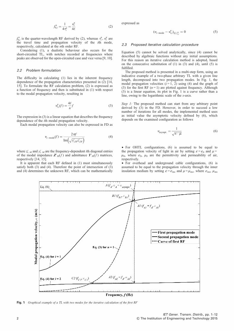
Fig. 1 Graphical example of a TL with two modes for the iterative calculation o

2

expressed as

(yi−mode − ynt,i)@ f nt,i= 0 (5)

2.3 Proposed iterative calculation procedure

Equation (5) cannot be solved analytically, since (4) cannot bedescribed by algebraic functions without any initial assumptions.For this reason an iterative calculation method is adopted, basedon the consecutive substitution of (1) in (3) and (4), until (5) isfulfilled.

The proposed method is presented in a multi-step form, using anindicative example of a two-phase arbitrary TL with a given linelength, decomposed into two propagation modes. In Fig. 1, themodal propagation velocities (i = 1, 2) using (4) and the graph of(3) for the first RF (n = 1) are plotted against frequency. Although(3) is a linear equation, its plot in Fig. 1 is a curve rather than aline, owing to the logarithmic scale of the x-axis.

Step 1: Τhe proposed method can start from any arbitrary pointderived by (3) in the FD. However, in order to succeed a lownumber of iterations for all modes, the implemented method usesas initial value the asymptotic velocity defined by (6), whichdepends on the examined configuration as follows

yasympt. =1��1 · m√ (6)

† For OHTL configurations, (6) is assumed to be equal tothe propagation velocity of light in air by setting ε = ε0 and μ =μ0, where ε0, μ0 are the permittivity and permeability of air,respectively.† For overhead and underground cable configurations, (6) isassumed to be equal to the propagation velocity through the innerinsulation medium by setting ε = εins and μ = μins, where εins, μins

f the first RF


Fig. 3 Typical OHTL transposition scheme

are the permittivity and permeability of the inner insulation layer,respectively.

Step 2: The υasympt. curve defines a horizontal line, which intersectsthe RF curve at point A with frequency fA calculated by substituting(6) in (3).Step 3: The frequency fA defines a vertical line, which intersects bothpropagation mode curves at points A1 ( fA1, υA1) and A2 ( fA2, υA2),where fA1 = fA2 = fA. The corresponding modal propagationvelocities are derived using (4), while the pul parameters arecalculated at fA. The modal decomposition in the denominator of(4) is readily performed using the conventional QR method.Step 4: Steps 2 and 3 are repeated for points A1 and A2 individually,using the corresponding modal propagation velocities instead of theasymptotic one of (6). Therefore in one iteration for point A1, that is,execution of both Steps 2 and 3, the algorithm results to B1 and B2.The latter point refers to the other propagation mode as calculatedusing (4) and is thus discarded and not indicated in Fig. 1.Similarly, point A2 moves to C2 with the corresponding C1 beingignored after the diagonalisation procedure.

The algorithm eventually terminates when the difference betweentwo subsequent frequencies for each mode is smaller than theuser-defined tolerance e, typically set to 1 Hz.

2.4 Effect of source and load impedances

The inclusion of the source impedance at the TL sending end (S) ofFig. 2 modifies the virtual TL length, and thus the calculated RFs [5].The proposed method can take into account this effect withoutaltering the previously presented iterative numerical scheme.

Let Z0 be the N × N diagonal matrix, containing the non-zerosource impedances connected to the energised conductors of theexamined TL. The lumped parameter matrix is converted to a puldistributed form in order to be considered as part of the TL. Thisis done by using (7), which associates the DF derived by a lumpedand a distributed electrical circuit [13]. Next, according to (8), thedistributed parameter matrix is added to the pul series impedancematrix of the TL. The result is used in (4) and is included in theiterative process

Z ′0(f ) =

2p

4

( )2

×Z0(f )

ℓ(7)

Z ′tot(f )= Z ′(f )+ Z ′

0(f ) (8)

Moreover, the effect of the load impedance (ZL) connected to the TLreceiving end (R) of Fig. 2 is inherently taken into account byclassifying two distinct cases for RFs, namely the open- andshort-circuit regions [5]. The limit between the two regions isdefined by the matched TL termination, where no reflections occur[10]. For each propagation mode, a termination impedance higherthan the modal characteristic one (Zn

ch,i) leads to a resonancebehaviour of the TL similar to the open-circuited case. Thereforethe spectral peaks and notches are observed at the frequenciesdictated by (9). On the other hand, for loads with values lowerthan the matched one, the TL behaviour is similar to the

Fig. 2 General configuration of an arbitrary N-phase TL


short-circuited case with the resonance extrema given by (10).

f nt,i =1, 3, 5, . . .{ } · f n0,i − peaks2, 4, 6, . . .{ } · f n0,i − notches

{for ZL . Zn

ch,i (9)

f nt,i =1, 3, 5, . . .{ } · f n0,i − notches2, 4, 6, . . .{ } · f n0,i − peaks

for ZL , Znch,i

{(10)

2.5 Integration of transposition and cross-bondingschemes

The OHTL transposition and cable cross-bonding techniques, usedfor balancing purposes, may slightly modify the TL propagationcharacteristics and thus the calculated RFs [18]. The proposedmethod can take into account this effect by adopting thehomogenisation approach of [19] for non-uniform TLs, which isaccurate enough and also guarantees smooth frequency variationof the propagation characteristics [20].

Considering the OHTL configuration of Fig. 3 and assuming equalline section lengths ℓA = ℓB = ℓC = ℓ/3

( ), the average pul series

impedance Z′ave.( f ) and shunt admittance Y′ave.( f ) matrices aregiven by

Z ′ave =

1

3(Z ′

A + Z ′B + Z ′

C)

= 1

3(Z ′

A + P · Z ′A · P−1 + P−1 · Z ′

A · P)(11)

Y ′ave =

1

3(Y ′

A + Y ′B + Y ′

C)

= 1

3(Y ′

A + P · Y ′A · P−1 + P−1 · Y ′

A · P)(12)

The permutation matrix operator P for the given transpositionscheme is defined as

P =0 1 00 0 11 0 0

⎡⎣

⎤⎦ (13)

The preceding matrices are used in (4) for the calculation of themodal propagation velocity, whereas the same procedure can alsobe applied to cross-bonded cables [13, 21].

However, the discontinuities associated with line conductortransposition and cable cross-bonding can also generate forward

3

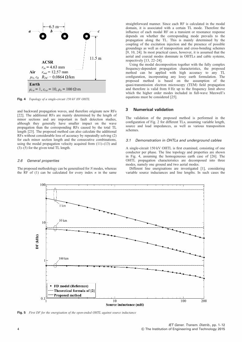
Fig. 4 Topology of a single-circuit 150 kV HV OHTL

and backward propagation waves, and therefore originate new RFs[22]. The additional RFs are mainly determined by the length ofminor sections and are important in fault detection studies,although they generally have smaller impact on the wavepropagation than the corresponding RFs caused by the total TLlength [23]. The proposed method can also calculate the additionalRFs without considerable loss of accuracy by repeatedly solving (2)for each minor section length and the consecutive combinations,using the modal propagation velocity acquired from (11)–(13) and(3)–(5) for the given total TL length.

2.6 General properties

The proposed methodology can be generalised for Nmodes, whereasthe RF of (1) can be calculated for every index n in the same

Fig. 5 First DF for the energisation of the open-ended OHTL against source ind

4

straightforward manner. Since each RF is calculated in the modaldomain, it is associated with a certain TL mode. Therefore theinfluence of each modal RF on a transient or resonance responsedepends on whether the corresponding mode prevails to thepropagation along the TL. This is mainly determined by thecoupling of the excitation injection and the presence of possiblegroundings as well as of transposition and cross-bonding schemes[9, 10, 24]. In most practical cases, however, it is assumed that theaerial and coaxial modes dominate in OHTLs and cable systems,respectively [13, 22–24].

Using the modal decomposition together with the fully complexfrequency-dependent propagation characteristics, the proposedmethod can be applied with high accuracy to any TLconfiguration, incorporating any lossy earth formulation. Theproposed method is based on the assumption of thequasi-transmission electron microscopy (TEM) field propagationand therefore is valid from 0 Hz up to the frequency limit abovewhich the higher order modes included in full-wave Maxwell’sequations must be considered [25].

3 Numerical validation

The validation of the proposed method is performed in theconfiguration of Fig. 2 for different TLs, assuming variable length,source and load impedances, as well as various transpositionschemes.

3.1 Demonstration in OHTLs and underground cables

A single-circuit 150 kV OHTL is first examined, consisting of oneconductor per phase. The line topology and properties are shownin Fig. 4, assuming the homogeneous earth case of [26]. TheOHTL propagation characteristics are decomposed into threemodes, namely one ground and two aerial modes.

Different line energisations are investigated [1], consideringvariable source inductances and line lengths. In such cases the

uctance


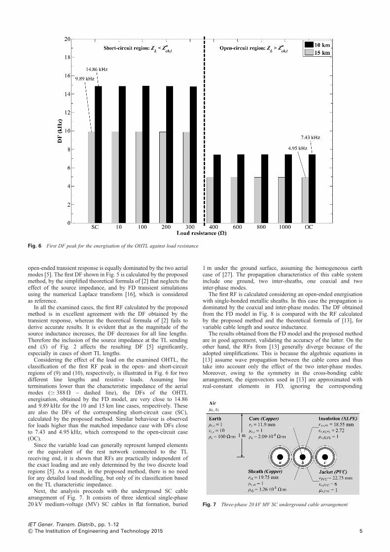
Fig. 6 First DF peak for the energisation of the OHTL against load resistance

Fig. 7 Three-phase 20 kV MV SC underground cable arrangement

open-ended transient response is equally dominated by the two aerialmodes [5]. The first DF shown in Fig. 5 is calculated by the proposedmethod, by the simplified theoretical formula of [2] that neglects theeffect of the source impedance, and by FD transient simulationsusing the numerical Laplace transform [16], which is consideredas reference.

In all the examined cases, the first RF calculated by the proposedmethod is in excellent agreement with the DF obtained by thetransient response, whereas the theoretical formula of [2] fails toderive accurate results. It is evident that as the magnitude of thesource inductance increases, the DF decreases for all line lengths.Therefore the inclusion of the source impedance at the TL sendingend (S) of Fig. 2 affects the resulting DF [5] significantly,especially in cases of short TL lengths.

Considering the effect of the load on the examined OHTL, theclassification of the first RF peak in the open- and short-circuitregions of (9) and (10), respectively, is illustrated in Fig. 6 for twodifferent line lengths and resistive loads. Assuming lineterminations lower than the characteristic impedance of the aerialmodes (≃ 388V – dashed line), the DFs of the OHTLenergisation, obtained by the FD model, are very close to 14.86and 9.89 kHz for the 10 and 15 km line cases, respectively. Theseare also the DFs of the corresponding short-circuit case (SC),calculated by the proposed method. Similar behaviour is observedfor loads higher than the matched impedance case with DFs closeto 7.43 and 4.95 kHz, which correspond to the open-circuit case(OC).

Since the variable load can generally represent lumped elementsor the equivalent of the rest network connected to the TLreceiving end, it is shown that RFs are practically independent ofthe exact loading and are only determined by the two discrete loadregions [5]. As a result, in the proposed method, there is no needfor any detailed load modelling, but only of its classification basedon the TL characteristic impedance.

Next, the analysis proceeds with the underground SC cablearrangement of Fig. 7. It consists of three identical single-phase20 kV medium-voltage (MV) SC cables in flat formation, buried


1 m under the ground surface, assuming the homogeneous earthcase of [27]. The propagation characteristics of this cable systeminclude one ground, two inter-sheaths, one coaxial and twointer-phase modes.

The first RF is calculated considering an open-ended energisationwith single-bonded metallic sheaths. In this case the propagation isdominated by the coaxial and inter-phase modes. The DF obtainedfrom the FD model in Fig. 8 is compared with the RF calculatedby the proposed method and the theoretical formula of [13], forvariable cable length and source inductance.

The results obtained from the FD model and the proposed methodare in good agreement, validating the accuracy of the latter. On theother hand, the RFs from [13] generally diverge because of theadopted simplifications. This is because the algebraic equations in[13] assume wave propagation between the cable cores and thustake into account only the effect of the two inter-phase modes.Moreover, owing to the symmetry in the cross-bonding cablearrangement, the eigenvectors used in [13] are approximated withreal-constant elements in FD, ignoring the corresponding

5

Fig. 8 First DF for the energisation of the open-ended underground cable against cable length

imaginary parts and the inherent frequency-dependent behaviour.These assumptions lead to errors in the calculation of themodal propagation velocities and the consequent RFs in cable

Fig. 9 Response of the energised phase for both OHTL configurations

6

configurations without cross-bonding arrangements, as the one inFig. 7, and especially when the source inductance is small. Incases of high source impedances, the DF is mainly affected by


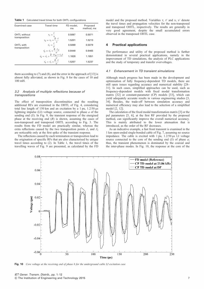
Table 1 Calculated travel times for both OHTL configurations

Examined case Travel time FD model,ms

Proposedmethod, ms

OHTL withouttransposition

t1 = ℓ

y0.5067 0.5071

t2 = t1 +2 · ℓy

1.5201 1.5213

OHTL withtransposition

t′1 = ℓ

y′0.5069 0.5079

t′2 = t′1 +2 · ℓCy′

0.8448 0.8465

t′3 = t′1 +2 · (ℓB + ℓC )

y′1.1828 1.1851

t′4 = t′1 +2 · ℓy′

1.5207 1.5237

them according to (7) and (8), and the error in the approach of [13] isalmost fully alleviated, as shown in Fig. 8 for the cases of 10 and100 mH.

3.2 Analysis of multiple reflections because oftranspositions

The effect of transposition discontinuities and the resultingadditional RFs are examined in the OHTL of Fig. 4, consideringtotal line length of 150 km and an excitation by a 1 pu, 1.2/50 μslightning impulse (LI) voltage source, connected to phase a of thesending end (S). In Fig. 9, the transient response of the energisedphase at the receiving end (R) is shown, assuming the cases ofnon-transposed and transposed OHTL according to Fig. 3. Theresults from the FD model are practically similar, whereas theextra reflections caused by the two transposition points J1 and J2are noticeable only at the first spike of the transient response.

The reflections caused by each termination or transposition lead tothe origination of specific RFs that are also characterised by uniquetravel times according to (2). In Table 1, the travel times of thetravelling waves of Fig. 9 are presented, as calculated by the FD

Fig. 10 Core voltage at the receiving end of phase b for the underground cable


model and the proposed method. Variables t, t′ and υ, υ′ denotethe travel times and propagation velocities for the non-transposedand transposed OHTL, respectively. The results are generally invery good agreement, despite the small accumulated errorsobserved in the transposed OHTL case.

4 Practical applications

The performance and utility of the proposed method is furtherdemonstrated in several practical applications, namely in theimprovement of TD simulations, the analysis of PLC applicationsand the study of temporary and transfer overvoltages.

4.1 Enhancement in TD transient simulations

Although much progress has been made in the development andoptimisation of fully frequency-dependent TD models, there arestill open issues regarding accuracy and numerical stability [28–31]. In such cases, simplified approaches can be used, such asfrequency-dependent models with fixed modal transformationmatrix [32] or constant-parameter (CP) models [33], which canyield adequately accurate results in various engineering studies [3,34]. Besides, the trade-off between simulation accuracy andnumerical efficiency may also lead to the selection of a simplifiedmodel [2, 12].

The calculation of the fixed modal transformation matrix [3] or thepul parameters [5, 6], at the first RF provided by the proposedmethod, can significantly improve the overall numerical accuracy.This is mainly attributed to the lower attenuation that isintroduced, as the order of the RF decreases.

As an indicative example, a fast front transient is examined in the1 km open-ended single-bonded cable of Fig. 7, assuming no sourceimpedance. The cable is excited with 1 pu, 1.2/50 μs LI voltagesource connected to the core of the sending end (S) of phase a;thus, the transient phenomenon is dominated by the coaxial andthe inter-phase modes. In Fig. 10, the response at the core of the

LI excitation case

7

Fig. 11 Experimental setup arrangement of a single-phase 20 kV MV SCcable on the ground surface

receiving end (R) is plotted for phase b, as calculated by the FD andthe CP TD model. The pul parameters for the latter are calculated at23.86 and 44.14 kHz according to the theoretical formula of [13] andthe proposed method, respectively.

The results obtained from the CP TD model, considering 44.14kHz as the DF of the transient response, are in good agreementwith the corresponding derived by the FD model. The frequencyof 23.86 kHz seems to introduce a lower attenuation and a phaseshift, which can be clearly observed after the first 100 μs of thetransient response.

4.2 PLC analysis

The accurate calculation of the frequencies at which the TLresonance extrema occur, using the proposed method, cangenerally enhance the selection of the optimal frequency band forthe transmission of signal in PLC applications [9–11].

Fig. 12 Voltage at the receiving end of the open-ended cable lying on the groun

a Coaxial mode excitationb Ground mode excitation

8

As an application, the laboratory experimental setup of Fig. 11 isconsidered, consisting of 180 m, 20 kV single-phase SC cable on theground surface. The cable electromagnetic and geometric propertiesare properly adjusted to accurately model the cable parameters [35].

Two types of single-phase injection are used for the excitation ofthe two cable propagation modes, based on Fig. 2. For the coaxialmode, the source is connected between the core and the sheath atthe sending end (S) of the cable, whereas for the ground modeboth the core and the sheath are simultaneously excited [10, 24].A sinusoidal signal generator is connected to the sending end (S)and an oscilloscope records the signal waveforms at bothopen-ended cable ends. A frequency scan is performed in therange of 1 kHz–1 MHz, whereas each measurement is repeated512 times and averaged in order to increase the signal-to-noise(SNR) ratio.

In Fig. 12, the recorded signal at the receiving end (R) is shown forthe two source excitations. In both figures the spectral peaks andnotches are denoted and correlated with the corresponding RFs of(1). It is evident that the ground mode excitation exhibits moreresonance extrema. This is because of the lower propagationvelocity compared to the corresponding coaxial mode in theexamined frequency range, which results in a smallerquarter-wavelength RF according to (2). Furthermore, forfrequencies higher than 150 kHz, the spectral peaks of the groundmode excitation exhibit lower values than those of the coaxialmode case, owing to the higher attenuation constant of the groundmode in this frequency range.

The measured RFs indicated in Fig. 12 are first compared inTable 2 with the corresponding RFs calculated using the proposedmethod. Next, the first RF is further investigated in Table 3, wherethe experimental excitation of the coaxial mode is repeated fordifferent lumped inductances and resistances connected to thesending end (S) of the open-ended cable core. For both test cases,the results from the proposed method are in good agreement withthe corresponding from field tests, validating the accuracy of the

d surface


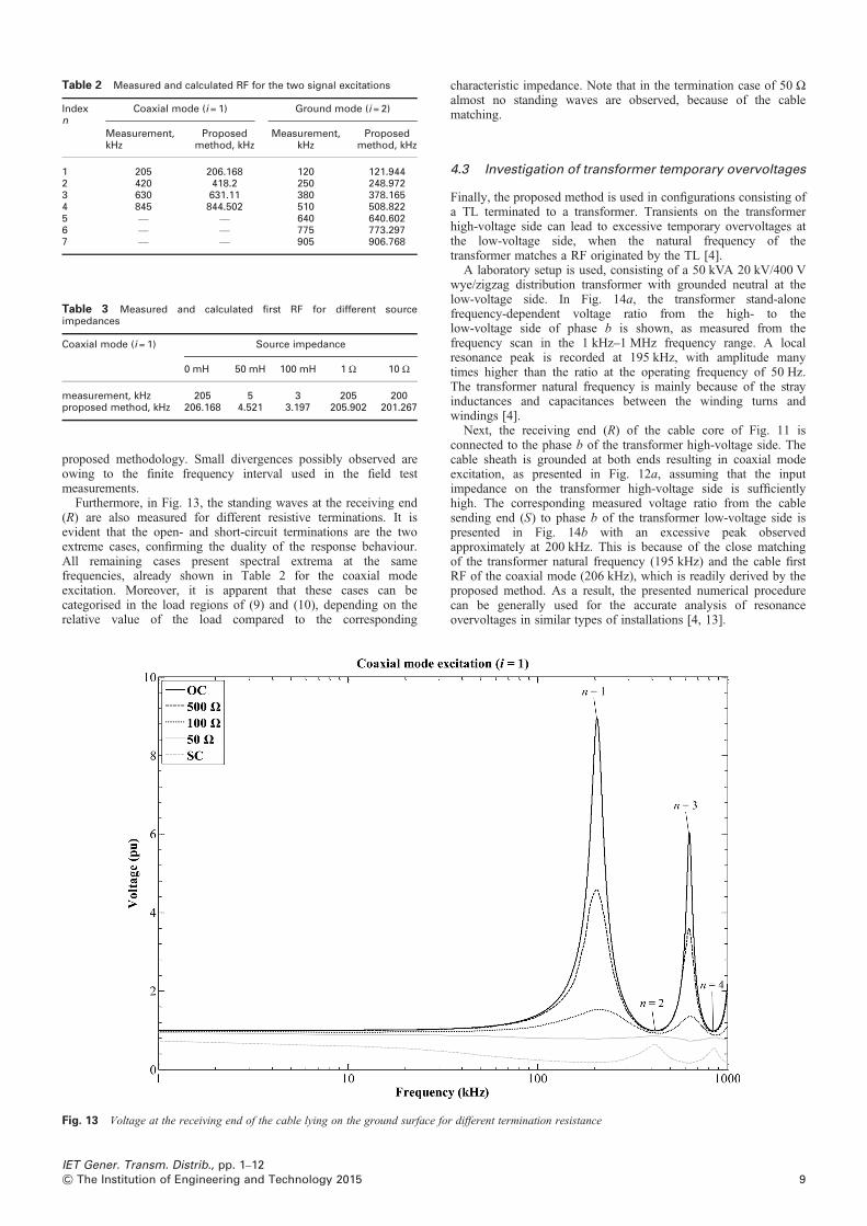
Table 3 Measured and calculated first RF for different sourceimpedances

Coaxial mode (i = 1) Source impedance

0 mH 50 mH 100 mH 1 Ω 10 Ω

measurement, kHz 205 5 3 205 200proposed method, kHz 206.168 4.521 3.197 205.902 201.267

Table 2 Measured and calculated RF for the two signal excitations

Indexn

Coaxial mode (i = 1) Ground mode (i = 2)

Measurement,kHz

Proposedmethod, kHz

Measurement,kHz

Proposedmethod, kHz

1 205 206.168 120 121.9442 420 418.2 250 248.9723 630 631.11 380 378.1654 845 844.502 510 508.8225 — — 640 640.6026 — — 775 773.2977 — — 905 906.768

proposed methodology. Small divergences possibly observed areowing to the finite frequency interval used in the field testmeasurements.

Furthermore, in Fig. 13, the standing waves at the receiving end(R) are also measured for different resistive terminations. It isevident that the open- and short-circuit terminations are the twoextreme cases, confirming the duality of the response behaviour.All remaining cases present spectral extrema at the samefrequencies, already shown in Table 2 for the coaxial modeexcitation. Moreover, it is apparent that these cases can becategorised in the load regions of (9) and (10), depending on therelative value of the load compared to the corresponding

Fig. 13 Voltage at the receiving end of the cable lying on the ground surface fo


characteristic impedance. Note that in the termination case of 50 Ωalmost no standing waves are observed, because of the cablematching.

4.3 Investigation of transformer temporary overvoltages

Finally, the proposed method is used in configurations consisting ofa TL terminated to a transformer. Transients on the transformerhigh-voltage side can lead to excessive temporary overvoltages atthe low-voltage side, when the natural frequency of thetransformer matches a RF originated by the TL [4].

A laboratory setup is used, consisting of a 50 kVA 20 kV/400 Vwye/zigzag distribution transformer with grounded neutral at thelow-voltage side. In Fig. 14a, the transformer stand-alonefrequency-dependent voltage ratio from the high- to thelow-voltage side of phase b is shown, as measured from thefrequency scan in the 1 kHz–1 MHz frequency range. A localresonance peak is recorded at 195 kHz, with amplitude manytimes higher than the ratio at the operating frequency of 50 Hz.The transformer natural frequency is mainly because of the strayinductances and capacitances between the winding turns andwindings [4].

Next, the receiving end (R) of the cable core of Fig. 11 isconnected to the phase b of the transformer high-voltage side. Thecable sheath is grounded at both ends resulting in coaxial modeexcitation, as presented in Fig. 12a, assuming that the inputimpedance on the transformer high-voltage side is sufficientlyhigh. The corresponding measured voltage ratio from the cablesending end (S) to phase b of the transformer low-voltage side ispresented in Fig. 14b with an excessive peak observedapproximately at 200 kHz. This is because of the close matchingof the transformer natural frequency (195 kHz) and the cable firstRF of the coaxial mode (206 kHz), which is readily derived by theproposed method. As a result, the presented numerical procedurecan be generally used for the accurate analysis of resonanceovervoltages in similar types of installations [4, 13].

r different termination resistance

9

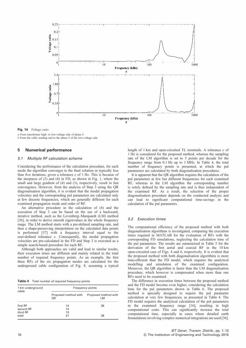
Fig. 14 Voltage ratio

a From transformer high- to low-voltage side of phase bb From the cable sending end to the phase b of the low-voltage side

5 Numerical performance

5.1 Multiple RF calculation scheme

Considering the performance of the calculation procedure, for eachmode the algorithm converges to the final solution in typically lessthan five iterations, given a tolerance e of 1 Hz. This is because ofthe steepness of (3) and (4) in FD, as shown in Fig. 1, where thesmall and large gradient of (4) and (3), respectively, result in fastconvergence. However, from the analysis of Step 3 using the QRdiagonalisation algorithm, it is evident that the modal propagationvelocities and the corresponding pul parameters are calculated onlyat few discrete frequencies, which are generally different for eachexamined propagation mode and order of RF.

An alternative procedure in the calculation of (4) and theexecution of Step 3 can be based on the use of a backward,iterative method, such as the Levenberg–Marquardt (LM) method[36], in order to derive smooth eigenvalues in the whole frequencyrange. The LM method starts with a pre-defined sampling rate, andthen a shape-preserving interpolation on the calculated data pointsis performed [37] with a frequency interval equal to theuser-defined tolerance e. Consequently, the modal propagationvelocities are pre-calculated in the FD and Step 3 is executed as asimple search-based procedure for each RF.

Although both approaches are valid and lead to similar results,their execution times are different and mainly related to the totalnumber of required frequency points. As an example, the firstthree RFs of the six propagation modes are calculated for theunderground cable configuration of Fig. 8, assuming a typical

Table 4 Total number of required frequency points

1 km undergroundcable

Frequency points

Proposed method withQR

Proposed method withLM

first RF 14 36second RF 14third RF 13total 41 36

10

length of 1 km and open-circuited TL terminals. A tolerance e of1 Hz is considered for the proposed method, whereas the samplingrate of the LM algorithm is set to 5 points per decade for thefrequency range from 0.1 Hz up to 1 MHz. In Table 4, the totalnumber of frequency points is presented, at which the pulparameters are calculated by both diagonalisation procedures.

It is apparent that the QR algorithm requires the calculation of thepul parameters at few but different frequencies for each examinedRF, whereas in the LM algorithm the corresponding numberis solely defined by the sampling rate and is thus independent ofthe examined RF. As a result, the selection of the properdiagonalisation procedure depends on the conducted analysis andcan lead to significant computational time-savings in thecalculation of the pul parameters.

5.2 Execution times

The computational efficiency of the proposed method with bothdiagonalisation algorithms is investigated, comparing the executiontimes required in MATLAB for the evaluation of RFs with thecorresponding FD simulations, neglecting the calculation time ofthe pul parameters. The results are summarised in Table 5 for thederivation of the first aerial and coaxial RF in the 10 kmopen-circuited case of Figs. 4 and 6, respectively. It is evident thatthe proposed method with both diagonalisation algorithms is moretime-efficient than the FD model, which requires the analyticalmodelling and simulation of the examined configuration.Moreover, the QR algorithm is faster than the LM diagonalisationprocedure, which however is compensated when more than oneRFs need to be examined.

The difference in execution times between the proposed methodand the FD model become even higher, considering the calculationtime for the pul parameters shown in Table 6. The proposedmethod is specially designed to require the pul parametercalculation at very few frequencies, as presented in Table 4. TheFD model requires the analytical calculation of the pul parametersin the examined frequency range [16], resulting in highcomputational costs. This can significantly increase the totalcomputational time, especially in cases where detailed earthformulations involving complex numerical integrations are used [36].


Table 6 Additional calculation times of pul parameters

Configuration Time, s

Proposedmethod with QRat 14frequencies

Proposedmethod with LMat 36 frequencies

FD model at1000

frequencies

10 km OHTL with[26]

0.01 0.02 0.6

10 kmundergroundcable with [27]

0.04 0.1 2.8

Table 5 Indicative execution times

Configuration Time, s

Proposed methodwith QR

Proposed methodwith LM

FDmodel

10 km OHTL 0.04 1.05 12.4510 km undergroundcable

0.09 2.57 16.36

6 Conclusions

A new methodology is presented for the calculation of RFs inoverhead and underground TLs. The proposed algorithm is basedon a robust and rigorous iterative calculation scheme, using themodal decomposition theory. Contrary to the theoretical formulasof limited accuracy and applicability, the proposed method giveshighly accurate results when compared with the correspondingfrom FD transient simulations and laboratory field tests.

The distinct advantage of the proposed method is its ability tocalculate the RF of any order and propagation mode in astraightforward and fast-converging way, taking fully into accountthe frequency dependence of the TL configuration, the effect ofTL transpositions or cross-bondings, the lumped elementsconnected to the TL terminals and the influence of the imperfectearth. In cases where only one RF calculation is required, the QRdiagonalisation algorithm is selected, enhancing the efficiency ofthe numerical technique and reducing the total computational timefor the pul parameters. On the other hand, in studies where thecalculation of multiple RFs is needed, the LM diagonalisationalgorithm is implemented, leading to a lower total number ofrequired frequency points. Both numerical approaches guarantee astable solution in few iterations and present smaller executiontimes compared to other traditional RF calculation methods,especially in cases involving complex lossy earth representations.

The accurate knowledge of RFs is important in a series of powersystems applications. The use of RFs can enhance the application ofsimplified TD models in TL lightning and switching overvoltagestudies, which are generally faster and less prone to numericalstability issues, allowing also the users to have a better insight inthe overall simulation process. The proposed method can alsocontribute to the comprehensive investigation of the channelcharacteristics of different TL types over a vast frequency range,which is of utmost importance to the design of PLC applications,as well as to the study of TL temporary overvoltages in thepresence of transformers or shunt reactors.

7 Acknowledgments

The authors gratefully acknowledge the contributions of Prof. P.N.Mikropoulos and Lect. G.T. Andreou for their help in conductingthe experimental tests. The work of A.I. Chrysochos is supportedby the Alexander S. Onassis Public Benefit Foundation via a meritscholarship between 2012 and 2015. The work of T.A.


Papadopoulos is supported by the ‘IKY Fellowships of Excellencefor Postgraduate Studies in Greece – Siemens Program’.

8 References

1 CIGRE Working Group 02 (SC33): ‘Guidelines for representation of networkelements when calculating transients’, 1990

2 Ametani, A., Kawamura, T.: ‘Amethod of a lightning surge analysis recommendedin Japan using EMTP’, IEEE Trans. Power Deliv., 2005, 20, (2), pp. 867–875

3 Soloot, A.H., Bahirat, H.J., Høidalen, H.K., Gustavsen, B., Mork, B.A.:‘Investigation of resonant overvoltages in offshore wind farms – Modeling andprotection’. IPST 2013, Vancouver, Canada, 2013

4 Gustavsen, B.: ‘Study of transformer resonant overvoltages caused bycable-transformer high-frequency interaction’, IEEE Trans. Power Deliv., 2010,25, (2), pp. 770–779

5 Kaloudas, Ch.G., Papadopoulos, T.A., Papagiannis, G.K.: ‘Spectrum analysis oftransient responses of overhead transmission lines’. UPEC 2010, Cardiff, Wales,2010

6 Chrysochos, A.I., Papadopoulos, T.A., Papagiannis, G.K.: ‘Improved time-domainmodeling of underground cables’. UPEC 2011, Soest, Germany, 2011

7 Colla, L., Lauria, S., Gatta, F.M.: ‘Temporary overvoltages due to harmonicresonance in long EHV cables’. IPST 2007, Lyon, France, 2007

8 Arrillaga, J., Smith, B.C., Watson, N.R., Wood, A.R.: ‘Power system harmonicanalysis’ (Wiley, 1997)

9 Papadopoulos, T.A., Kaloudas, Ch.G., Chrysochos, A.I., Papagiannis, G.K.:‘Application of narrowband power-line communication in medium-voltage smartdistribution grids’, IEEE Trans. Power Deliv., 2013, 28, (2), pp. 981–988

10 Papadopoulos, T.A., Chrysochos, A.I., Papagiannis, G.K.: ‘Narrowband power linecommunication: medium voltage cable modeling and laboratory experimentalresults’, Int. J. Electr. Power Syst. Res., 2013, 102, pp. 50–60

11 Milioudis, A.N., Andreou, G.T., Labridis, D.P.: ‘Enhanced protection scheme forsmart grids using power line communications techniques – Part I: Detection ofhigh impedance fault occurrence’, IEEE Trans. Smart Grid, 2012, 3, (4),pp. 1621–1630

12 Manitoba HVDC Research Centre: ‘EMTDC user’s guide – Transient analysis forPSCAD power system simulation’ (Manitoba, 2010)

13 Ohno, T., Bak, C.L., Ametani, A., Wiechowski, W., Sørensen, T.K.: ‘Derivationof theoretical formulas of the frequency component contained in theovervoltage related to long EHV cables’, IEEE Trans. Power Deliv., 2012, 27,(2), pp. 866–876

14 Wedepohl, L.M.: ‘Application of matrix methods to the solution of travelling-wavephenomena in polyphase systems’, Proc. Inst. Electr. Eng., 1963, 110, (12),pp. 2200–2212

15 Wedepohl, L.M., Wilcox, D.J.: ‘Transient analysis of underground power-transmission systems: System-model and wave-propagation characteristics’, Proc.Inst. Electr. Eng., 1973, 120, (2), pp. 253–260

16 Moreno, P., Ramirez, A.: ‘Implementation of the numerical Laplace transform: Areview’, IEEE Trans. Power Deliv., 2008, 23, (4), pp. 2599–2609

17 Ametani, A.: ‘A general formulation of impedance and admittance of cables’, IEEETrans. Power Appar. Syst., 1980, PAS-99, (3), pp. 902–910

18 Ametani, A., Nagaoka, N., Baba, Y., Ohno, T.: ‘Power system transients – theoryand applications’ (CRC Press, 2014)

19 Dang, N.D.: ‘Transient performance of crossbonded cable systems’. PhD thesis,UMIST, 1972

20 Brandão Faria, J.A., Guerreiro das Neves, M.V.: ‘Nonuniform three-phase powerlines: resonance effects due to conductor transposition’, Int. J. Electr. PowerEnergy Syst., 2004, 26, pp. 103–110

21 Indulkar, C.S., Kumar, P., Kothari, D.P.: ‘Modal propagation and sensitivity ofmodal quantities in crossbonded cables’, Proc. Inst. Electr. Eng., 1983, 130, (6),pp. 278–284

22 Gudmundsdottir, U.S., Gustavsen, B., Bak, C.L., Wiechowski, W.: ‘Field test andsimulation of a 400-kV cross-bonded cable system’, IEEE Trans. Power Deliv.,2011, 26, (3), pp. 1403–1410

23 Jensen, C.F., Gudmundsdottir, U.S., Bak, C.L., Abur, A.: ‘Field test and theoreticalanalysis of electromagnetic pulse propagation velocity on crossbonded cablesystems’, IEEE Trans. Power Deliv., 2014, 29, (3), pp. 1028–1035

24 Chrysochos, A.I., Papadopoulos, T.A., Papagiannis, G.K.: ‘Analysis of thepropagation characteristics of single-core cables from experimental results usingmodal decomposition’. Int. University Power Engineering Conf., Dublin, Ireland,2013

25 Theethayi, N., Baba, Y., Rachidi, F., Thottappillil, R.: ‘On the choice betweentransmission line equations and full-wave Maxwell’s equations for transientanalysis of buried wires’, IEEE Trans. Electromagn. Compat., 2008, 50, (2),pp. 347–357

26 Wise, W.H.: ‘Potential coefficients for ground return circuits’, Bell Syst. Tech. J.,1948, 27, pp. 365–372

27 Sunde, E.D.: ‘Earth conduction effects in transmission systems’ (Dover, New York,1968)

28 Gustavsen, B., Irwin, G., Mangerlod, R., Brandt, D., Kent, K.: ‘Transmission linemodels for the simulation of interaction phenomena between parallel AC and DCoverhead lines’. Int. Power System Transactions Conf., Budapest, Hungary, 1999

29 Ramirez, A., Iravani, R.: ‘Enhanced fitting to obtain an accurate DC response oftransmission lines in the analysis of electromagnetic transients’, IEEE Trans.Power Deliv., 2014, 29, (6), pp. 2614–2621

30 Kocar, I., Mahseredjian, J., Olivier, G.: ‘Improvement of numerical stability for thecomputation of transients in lines and cables’, IEEE Trans. Power Deliv., 2010, 25,(2), pp. 1104–1111

11

31 Gustavsen, B.: ‘Avoiding numerical instabilities in the universal line model by atwo-segment interpolation scheme’, IEEE Trans. Power Deliv., 2013, 28, (3),pp. 1643–1651

32 Marti, J.R.: ‘Accurate modeling of frequency-dependent transmission lines inelectromagnetic transient simulations’, IEEE Trans. Power Appar. Syst., 1982,PAS-101, (1), pp. 147–157

33 Dommel, H.W., Meyer, W.S.: ‘Computation of electromagnetic transients’. Proc.IEEE, 1974, vol. 62, no. 7

34 Kaloudas, Ch.G., Papadopoulos, T.A., Gouramanis, K.V., Stasinos, K.,Papagiannis, G.K.: ‘Methodology for the selection of long-medium-voltage

12

power cable configurations’, IET Gener. Transm. Distrib., 2013, 7, (5),pp. 526–536

35 Gustavsen, B., Martinez, J.A., Durbak, D.: ‘Parameter determination for modelingsystem transients – Part II: Insulated cables’, IEEE Trans. Power Deliv., 2005, 20,(3), pp. 2045–2050

36 Chrysochos, A.I., Papadopoulos, T.A., Papagiannis, G.K.: ‘Robust calculation offrequency-dependent transmission line transformation matrices using the Levenberg–Marquardt method’, IEEE Trans. Power Deliv., 2014, 29, (4), pp. 1621–1629

37 Fritsch, F.N., Carlson, R.E.: ‘Monotone piecewise cubic interpolation’, SIAMJ. Numer. Anal., 1980, 17, pp. 238–246


Rigorous calculation method for resonance frequencies in ...

Documents

Transcript of Rigorous calculation method for resonance frequencies in ...