Noise levels of superconducting gravimeters at seismic frequencies

Noise levels of superconducting gravimeters at seismic frequencies

Dirk Banka1 andDavid Crossley2

1 British Geological Survey, Kingsley Dunham Centre, Nottingham, NG12 5GG, UK. E-mail: [email protected] Department of Earth andAtmospheric Sciences, Saint LouisUniversity, 3507LacledeAve, St. Louis, MO63103,USA.E-mail: [email protected]

Accepted 1999 May 10. Received 1999 April 30; in original form 1998 May 27

SUMMARYUntil recently superconducting gravimeters (SGs) have been used principally intidal studies (periods 6^24 hr) due to their high sensitivity and low drift rates. Thispaper considers the performance of these instruments as long-period seismometers,particularly in the normal mode band (periods 1^54 min). To judge their suitability inproviding useful information to seismology, it is important to determine their noisecharacteristics compared to other established instruments such as spring gravimeters.

We compare several continuously recording instruments: the SGs in Esashi (Japan),Wuhan (China), Strasbourg (France) and Cantley (Canada) and the spring gravimeterET-19 and seismometer STS-1 at the Black Forest Observatory (BFO, Germany).We also include non-permanent instruments, the SG102 at BFO as well as the ET-18in MetsÌhovi (Finland). The ¢ve quietest days out of the available records are stackedto obtain the power spectral density of the noise in the frequency band 0.05^20 mHz(50 s to 6 hr). Our reference is the New Low Noise Model designed for seismometers.Only at the BFO site were there several instruments that could be compared; even so, inorder to obtain the best individual data for each instrument the records selected werenot simultaneous.

The noise characteristics of the di¡erent instrument^site combinations are com-pared, leading to conclusions about site selection, instrument modi¢cations and therecent potential of SGs to contribute to seismic normal mode studies. We refer to ourprevious work on the seismic noise magnitude, a summary statistic derived from thepower spectral density which has been used to rank the performance of instrument^sitecombinations.

Key words: normal modes, seismic noise, superconducting gravimeter.

INTRODUCTION

Studies of the free oscillations of the Earth are based mainlyon seismometers and classical spring gravimeters, which areconnected in large networks such as IRIS (Smith 1987),GEOSCOPE (Romanowicz et al. 1984), IDA (Agnew et al.1986) and DWWSSN (Peterson & Hutt 1982). Due to theactivity of the Global Geodynamics Project (GGP; Crossley& Hinderer 1995), there is now a network of more than 15superconducting gravimeters (SGs), some of which have beenrecording for more than a decade. Despite the slow growth inSG installations over the last decade, it is unlikely that thisnetwork will reach the density of the established networks dueto limited ¢nancial and technical resources.Several studies have shown that SGs, as acceleration sensors,

can clearly record normal modes, e.g. ZÏrn et al. (1991), Kamal& Mansinha (1992), Richter et al. (1995a,b) and Banka &Crossley (1995). It is therefore worthwhile to investigate their

characteristics in this frequency band in comparison withestablished instruments such as spring gravimeters.Initially the SG was developed for investigations in the

low-frequency (tidal) band (Prothero & Goodkind 1972).The low drift and high sensitivity of their design is due to theextreme stability of the superconducting currents supplyingthe `magnetic' spring, compared to the metal alloy spring of aclassical gravimeter. The idea is now to use this sensitivity alsoto record the seismic normal modes and to contribute data tothe established networks. ZÏrn et al. (1991) and Richter et al.(1995a,b) have claimed that SGs have a higher noise levelthan LaCoste^Romberg spring gravimeters with electrostaticfeedback in this frequency range. In these studies, as well asour own, there are legitimate concerns about whether the noiselevels re£ect di¡erences between sites or di¡erences betweeninstruments. Naturally, our study is limited by having to acceptthe instruments sited where they were installed. Even within aparticular category of instrument (e.g. a single model of SG)

Geophys. J. Int. (1999) 139, 87^97

ß 1999 RAS 87

by guest on October 6, 2016

http://gji.oxfordjournals.org/D

ownloaded from

http://gji.oxfordjournals.org/

there are signi¢cant mechanical and electrical di¡erences thatwill a¡ect the noise levels we are trying to de¢ne.In the present study, the ambient site noise and the New Low

Noise Model (NLNM; Peterson 1993) are used as a referencesignal to give an estimation of the quality of the site^sensorcombination. With a single instrument at a site, it is notpossible to separate site noise from instrument noise; fromonly one site (BFO) did we have several instruments to com-pare. Our procedure was to choose data based on the lowestindividual noise spectra for single days, and it turned out thatthere were no common days when the data from two (or more)instruments were used. At other sites we made no attempt tochoose similar days; nevertheless, we are con¢dent in reachingseveral conclusions about the performance of the instrumentsand the contributions of site noise.Our study is complementary to the other aspects of

SG measurements; for example, it has been demonstratedrepeatedly (e.g. Goodkind et al. 1991; Hinderer et al. 1994) thatSGs have a very stable calibration, they have very small driftcompared to spring gravimeters, and they are very sensitive(high precision). Compared to most other spring gravimeters,except installations such as the ET-19 at BFO, which Richteret al. (1995a) showed to be of very high quality, and certainlycompared to seismometers, SGs yield the most accurate tidalamplitudes and phases. They are clearly the only type ofgravimeter that can compare over intervals of years withabsolute gravimeters (e.g. Lambert et al. 1995).

PROCESSING PROCEDURE

The processing procedure is fully described and evaluated inBanka et al. (1998); here it will be only brie£y summarized.Compared to the older seismic data, gravimeter data are usuallycontinuous, often for many years, and have to be processedto reduce the in£uence of long-period e¡ects (e.g. tides).Seismometers attenuate low frequencies by design, and the recentIRIS broad-band data sets are also much more continuousthan a few years ago. We apply the following processing stepsto the various data sets where possible.

(1) Amplitude calibration with a calibration factor extra-polated from the tidal band, usually obtained by comparisonwith absolute gravimeters or an indirect equivalent absolutemeasure.(2) Subtraction of the tides computed using an elastic

reference earth model.(3) Reduction of the in£uence of the air pressure with an

admittance factor extrapolated from the tidal band.(4) Subtraction of a best-¢tting ninth-degree polynomial to

eliminate the instrument drift and any residual tidal signal.(5) Windowing with a 10 per cent cosine bell window, and

padding by a factor of at least two before taking a fast Fouriertransform (FFT). A correction is made for the data taper,assuming a white noise spectrum, and the power spectraldensities are multiplied by a factor 2 to include the complexFFT at negative frequencies.(6) The amplitude spectrum is then smoothed by an 11-point

Parzen frequency window; this does not change the powerspectral density (PSD) estimates.

These steps provide an objective comparison between thedi¡erent instruments.

DATA ANALYSIS

Collection

At the beginning of 1995 we contacted several groupsinvolved with instruments and requested low-noise data for thecurrent study. One condition was that each data set shouldhave a length of at least 1 day. We requested several days ofdata, with particularly low noise, from the last four years.Details of the data sets can be found in Banka (1997). SGstation information is given in Crossley & Hinderer (1995)and in Wenzel et al. (1991), ZÏrn et al (1991) and Widmeret al. (1992) for the very quiet multipurpose Black ForestObservatory (BFO). All SGs are manufactured by GWRInstruments (San Diego).

Selection

The aim was to select data which have the lowest noise levelfor each instrument, as indicated above. From the databasesupplied by the operators (representing by no means all the SGsites available), those records were chosen with the leastnumber of steps, spikes, gaps, earthquakes and other obviousnoise sources such as atmospheric or oceanic noise.Steps can in principle be removed, but there is no reliable way

to estimate visually the amplitude of a step and it is dangerousto rely on automatic methods to remove steps completely(Crossley et al. 1993). As far as possible records with steps(and spikes) were therefore excluded.For most spectral analyses gaps have to be replaced by

simple mathematical functions or synthetic tides without noise.Because in our study the noise is the main component, it makesno sense to ¢ll a gap with synthetic noise.Earthquakes bring two problems. First, they can saturate the

sensor and this adds arti¢cial noise to the spectrum; second,the frequency content of seismic signals cannot always be dis-tinguished from site or instrument noise. However, as wasnoted in Banka (1997), a small earthquake adds insigni¢cantnoise to an otherwise quiet record.We very quickly established that the winter months are

not suitable for our study due to high atmospheric andoceanic noise. This was one of the reasons we did not ask forspeci¢c records, but for quiet records chosen by the operator. Aquiet time interval at one site can be unacceptable due toatmospheric or oceanic noise at another. Also, small localearthquakes and instrument disturbances have to be avoidedon an individual site or instrument basis.To achieve comparable conditions in terms of padding,

frequency sampling, etc., a ¢xed record length was chosen,which also makes it possible to stack the spectra to smoothindividual records. For convenience a 1 day record length waschosen.To summarize, our selection procedure was based partly on

operator expertise, since we asked for ¢ve quiet days for someof the stations, and partly on an objective measure where wehad access to su¤cient data ourselves. The latter circumstanceenabled us to reject days with obvious visual problems and thento compute the PSD of the remaining records. The ¢ve dayswith the lowest overall PSD were selected for each station(see Table 1), this number (5) being the largest given to us forone of the stations, for the ¢nal stack.

ß 1999 RAS, GJI 139, 87^97

88 D. Banka and D. Crossley



ownloaded from


Processing

Our attempt to treat the data equally failed because thesampling rates were di¡erent; therefore, the number of valuesin each record was di¡erent and thus also the padding. Formost stations we had the tidal record of the instrument, butfor two stations (Strasbourg and Esashi) only the mode out-put was available. This meant that there was an additionalampli¢cation factor with a non-uniform frequency responsethat had to be taken into account when computing andsubtracting the synthetic tides.Ideally, one should correct for the instrument response ¢rst,

before performing the tidal subtraction and the atmosphericcorrection, which most people assume is similar at seismicfrequencies to tidal frequencies. Because the mode outputresponse is somewhat uncertain, we could not correct for itaccurately enough to permit a pressure correction.The STS-1 seismometer has a frequency-dependent transfer

function that should be subtracted before doing any pro-cessing such as tidal subtraction and atmospheric pressuresubtraction.We did not apply this correction before processingand so did not subtract tides or correct for air pressure. Eventhough ZÏrn & Widmer (1995) have noted that air pressurecorrections were not as signi¢cant for the STS-1 as for theET-19 (the same instruments that we were using at BFO), an

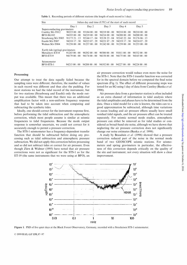
air pressure correction would reduce even more the noise forthe STS-1. Note that the STS-1 transfer function was correctedfor in the spectral domain before we computed the ¢nal noisespectrum (Fig. 1). The e¡ect of di¡erent processing steps wastested for an SG using 1 day of data from Cantley (Banka et al.1998).Air pressure data from a gravimeter station is often included

as an extra channel of information in tidal analysis wherethe tidal amplitudes and phases have to be determined from thedata. Once a tidal model for a site is known, the tides can to agood approximation be subtracted, although time variationsin ocean loading and air pressure e¡ects usually leave smallresidual tidal signals, and the air pressure e¡ect can be treatedseparately. For seismic normal mode studies, atmosphericpressure can either be removed as for tidal studies or con-sidered as broad-band site noise, although we have shown thatneglecting the air pressure correction does not signi¢cantlychange our noise estimates (Banka et al. 1998).A study by Beauduin et al. (1996) showed that a pressure

correction reduced part of the noise in the normal modeband of two GEOSCOPE seismic stations. For seismo-meters and spring gravimeters in particular, the e¡ective-ness of this correction depends critically on the quality ofthe site and instrument; not every situation will show a clearimprovement.

Table 1. Recording periods of di¡erent stations (the length of each record is 1 day).

Site Julian day and time (UTC) of the start of each record

Day 1 Day 2 Day 3 Day 4 Day 5Superconducting gravimetersCantley SG-T012 90223 00 : 00 93184 00 : 00 90219 00 : 00 90218 00 : 00 90210 00 : 00BFO-SG102 94193 00 : 00 94219 00 : 00 94216 00 : 00 94208 00 : 00 94200 00 : 00Strasbourg SG-T005 91173 21 : 13 92144 17 : 04 92138 23 : 04 92142 22 : 04 91176 06 : 13Esashi SG-T007 94218 17 : 30 94223 07 : 29 94221 07 : 29 94219 17 : 30 94224 07 : 29Wuhan SG-T004 91258 00 : 00 91257 00 : 00 91242 00 : 00 91259 00 : 00 91255 00 : 00

Earth tide (spring) gravimetersMetsa« hovi ET18 91243 00 : 00 90292 00 : 00 90300 00 : 00 91011 00 : 00 90332 00 : 00BFO-ET19 94179 00 : 00 94174 00 : 00 94158 00 : 00 94175 00 : 00 94165 00 : 00

SeismometerBFO-STS-1 94215 00 : 00 94208 00 : 00 94192 00 : 00 94227 00 : 00 94224 00 : 00

Figure 1. PSD of ¢ve quiet days at the Black Forest Observatory, Germany, recorded with a Streckeisen STS-1 seismometer.

ß 1999 RAS,GJI 139, 87^97

89Noise levels of superconducting gravimeters



ownloaded from


Calibration

Gravimeter calibration factors were originally determined bycomparisons with either raw data from absolute gravimeters(Hinderer et al. 1991; Bower et al. 1991) or tidal analysis of datafrom relative gravimeters (Sato et al. 1994). The disadvantageof both methods is the dominance of the M2 tide (&12 hrperiod) that determines the single calibration factor.We assume that at seismic frequencies the calibration

factor can be extrapolated from the appropriate ¢lter functionssupplied by the manufacturer (GWR-Manual 1985). Richter(1995) showed that the calibration of spring gravimeterLCR-D009 was within 1 per cent from 200 to 900 s, butno direct extension to tidal frequencies has yet been carriedout for any gravimeter. The transfer functions of the STS-1seismometers are similar, as they are for the SGs, so it isunlikely that assumptions about this extrapolation will a¡ectour conclusions.The additional ampli¢cation of the mode output requires an

adjustment of the calibration factor, and the high-pass ¢lterused in Strasbourg and Esashi means that frequencies lowerthan 0.833 mHz are not reliable.The output of theWielandt STS-1 seismometer is essentially

a velocity, but with a non-constant transfer function, givenin the frequency domain; the output can be converted toacceleration. In this case the calibration was the last step.

Subtraction of synthetic tides

As mentioned, we subtracted synthetic tides for an elasticreference earth model using the program GTIDE (Merriam1992), including the free core nutation correction, using3070 waves, but without local or ocean tides. The residualshad amplitudes of 1^2 ]gal (10^20 nm s{2). For mode data,the synthetic tides were subtracted and reduced by a factor of1/213 to take into account the high-pass mode ¢lter. As indi-cated earlier, for the STS-1, due to the frequency-dependenttransfer function that rolls o¡ the tidal frequencies, we did notsubtract a model synthetic tide; tidal residuals were presentonly at the 1^2 ]gal level.

Air pressure correction

For tidal analysis the air pressure correction is important.Hourly atmospheric pressure typically has a standard deviationof *10 mbar, which leads (see below) to gravity variations of*3 ]gal. These are signi¢cant in high-precision tidal analysiswhen looking for small waves. In gravimetry, pressure is oftenrecorded at a much lower sampling rate than the gravity signaland occasionally it may not be recorded at all (although thisis less and less common). We (see Banka 1997) con¢rm theexperience of other groups (e.g. ZÏrn & Widmer 1995) thatthe air pressure can in£uence noise in the normal mode band.Obviously, this correction will be more important wherethe site and instrument quality are high. Only where the datawere available, the correlation with gravity was high and theadmittance was reasonable did we perform an air pressurecorrection.For Esashi, Sato et al. (1994) gave an admittance of

{0.373 ]gal mbar{1 ({3:73 nm s{2 hPa{1); for Cantley itis {0:322 ]gal mbar{1 (Hinderer et al. 1994), and Richter

et al. (1995a) obtained {0:328 ]gal mbar{1 for the SG102and {0:337 ]gal mbar{1 for the ET-19. Although at BFO theinstruments are at the same site, they seem to have a slightlydi¡erent admittance factor, even though this should notdepend on the type of instrument used. For most data sets anominal admittance of {0:3 ]gal mbar{1 should be suitablefor the air pressure correction in the seismic band.

Residual tides and instrumental drift

A ninth-degree polynomial is used to remove the remaininglow frequencies due to tides and instrument drift. Experimentswere made using lower-degree polynomials, but undesirablelarge amplitudes were left at the beginning and end of theresidual series.With a ninth-degree polynomial four oscillationscan be modelled, which corresponds to an oscillation with a6 hr periodöat the limit of the frequency range for this study.

Spectral analysis

We took the FFTs, as discussed previously, of the ¢ve quietestdays for each station (Table 1). These were than averagedbefore computing the smoothed PSD.

RESULTS

We discuss themean PSD of all the instrument^site combinationsin three period ranges.

Short periods: 2 s^5 min (3.3^500 mHz)

This part of the spectrum includes the two minima of theNLNM, the increasing noise at high frequencies and in somecases the roll-o¡ of the anti-aliasing ¢lter.The NLNM and the spectrum of the STS-1 (Fig. 1) agree

very well; even the small maximum around 8 mHz is visible.At higher frequencies the anti-aliasing ¢lter begins around45 mHz but this is not apparent for either the seismometeror the NLNM as they are compensated by their transferfunctions. The small maximum is also visible in the record ofthe spring gravimeter ET-19 at BFO (Fig. 2).All the other sites are too noisy to show the small maxi-

mum between 5 and 10 mHz and the PSDs are more or less £atin this frequency range. The standard, original GWR tidal ¢lterhas a corner frequency at *12.5 mHz (80 s), so there is noadvantage in recording at a sampling interval shorter than 16 s.The Esashi record (Fig. 3) shows a strong peak at*10 mHz,

and a similar peak can be seen in the Cantley record (Fig. 4).These peaks are undoubtedly the sphere resonance of SGs(ZÏrn et al. 1995), this mode being excited by horizontalarti¢cial disturbances such as helium re¢lls. Nevertheless, wechose to include one of these days for Cantley because its noiselevel is otherwise very low. At Esashi this resonant mode ispresent in all our records and, according to R. Reinemannat GWR (personal communication, 1995), is continuouslyexcited by an interaction between the refrigeration tubes andthe gravimeter.In Cantley only the tide output is sampled, but with a

modi¢ed analogue ¢lter (with a corner period of 6.2 s) topermit full use of the 1 s data sampling. These data are ¢ltered

ß 1999 RAS, GJI 139, 87^97




ownloaded from


Figure 2. PSD of ¢ve quiet days at the Black Forest Observatory, Germany, recorded with the LaCoste^Romberg Earth tide gravimeter ET-19.

Figure 3. PSD of ¢ve quiet days at Esashi, Japan, recorded with SG-T007.

Figure 4. PSD of ¢ve quiet days at Cantley, Canada, recorded with SG-T012.

ß 1999 RAS,GJI 139, 87^97




ownloaded from


with a Chebyshev ¢lter (with a cut-o¡ period of 40 s) anddecimated to 10 s. The e¡ect of the Chebyshev ¢lter with acorner frequency of 25 MHz can be seen in Fig. 4.In Wuhan (Fig. 5) and MetsÌhovi (Fig. 6) di¡erent data

acquisition systems were used. The A/D conversion per-formed an integration directly on the raw analogue data,without any ¢lter. Subsequently, the data were ¢ltered with adigital low-pass ¢lter with a cut-o¡ period of 30 s and stored at20 s samples (Asch 1988). Because there is no analogue anti-aliasing ¢lter, phase shifts are avoided. The feedback system ofthe ET-18 has a time constant of *10 s, so that there are onlyminor problems to be expected. There are, however, a numberof problems with 10 s integration that can be shown tocause aliasing and increased noise levels in our processing. Fordetails we refer to Banka (1997).

Intermediate periods: 5^24 min (0.69^3.3 mHz)

It is obvious that Wuhan, China, is the noisiest site (Fig. 7),which con¢rms the work of Jentzsch &Melzer (1991). The datafor a typical day shows a dramatic di¡erence between the day

and night hours (Banka 1997). At night the noise level is com-parable to the SG record at BFO, whereas during the day largeone-sided spikes dominate the record. This noise is of culturalorigin and is the reason this instrument has now been relocatedto a new site outside the city (Hsu, personal communication,1997).In the records of Esashi, MetsÌhovi and Strasbourg such

clues are not visible and one must assume that these noiselevels (Figs 3, 6 and 8) are due to their locations. For example,in comparing Strasbourg (Fig. 8) with MetsÌhovi (Fig. 6), onecan see that they have similar medium noise levels, but one isan SG and the other a spring gravimeter. It needs to be statedthat the full-sized SG instrument at Strasbourg used in thisstudy has now been replaced by a newer compact SG withmuch improved noise characteristics. A new analysis for thissite should be performed, and we anticipate that Strasbourgwould probably now be included with BFO and Cantley(below) as a low-noise site.The last group, BFO and Cantley, can be called the low

noise sites (Fig. 9). If several instruments are recording atthe same site, one assumes the noise di¡erences are generated

Figure 5. PSD of 5 quiet days at Wuhan, China, recorded with SG-T004.

Figure 6. PSD of ¢ve quiet days at MetsÌhovi, Finland, recorded with Lacoste^Romberg Earth tide gravimeter ET-18.

ß 1999 RAS, GJI 139, 87^97




ownloaded from


by instrumental e¡ects, as should be the case for the SG andspring gravimeters at BFO. The SG102 was added to theinstallation at BFO for only a short time period. This SG has ahalf-sized sensor with a 50 l dewar (the standard instrumentshave 200 l dewars), but without a refrigeration system, andis supposed to meet the same speci¢cations for sensitivity,

stability and drift as the large instruments. This was a proto-type instrument, at that time still under evaluation (Richteret al. 1995a,b), and was manufactured with a smaller sensor ina set of only three (SG101, 102 and 103). The next generationof compact instruments (e.g. designated C024, van Dam &Francis 1998) all have a full-size (original) one inch sphere.

Figure 7. Comparison of mean PSD in various frequency bands from a stack of ¢ve quiet days, all noise levels.

Figure 8. PSD of ¢ve quiet days at Strasbourg, France, recorded by SG-T005.

ß 1999 RAS,GJI 139, 87^97




ownloaded from


Assuming the same NLNM (shown in Figs 1^10) at bothCantley and BFO, one might conclude that the SG at BFOhas a higher instrument noise than that at Cantley, probablydue to the fact that the sensor sizes are di¡erent. If so,this would indicate that the larger sensor is less noisythan SG102. Nevertheless, the Cantley instrument still hasa higher noise level than the spring instruments at BFO, as

can be seen by comparing the stacked spectra shown in Figs 1and 4 (plotted to the same scale). The average PSD levelin the selected band is obviously di¡erent from instrumentto instrument. As an example, comparing the BFO andMetsÌhovi spring gravimeters, small signals, clearly visibleat BFO around 1 mHz, would be below the noise level atMetsÌhovi.

Figure 9. Comparison of mean PSD in various frequency bands from a stack of ¢ve quiet days, low noise levels.

Figure 10. PSD of ¢ve quiet days at the Black Forest Observatory, Germany, recorded with GWR superconducting gravimeter SG-102.

ß 1999 RAS, GJI 139, 87^97




ownloaded from


The spectrum of ET-19 shows peaks at 0.943 and 0.813 mHz(21 and 17 min respectively) that come from one of the ¢veselected days following the deep Bolivian earthquake (6.9 mb).This earthquake occurred 5 days previously (94160, see Table 1).These are the high-Q modes 3S1 and 0S0 respectively that werestrongly excited due to the depth of the event. The other modeshad already decayed into the residual signal, which showsthat the tail of a large deep earthquake does not necessarilycontribute to a high broad-band noise level. This day was stillone of the quietest available by our PSD criterion.

Long periods: 24 min^5.5 hr (0.05^0.69 mHz)

In this frequency band between the tides and the middle ofthe normal mode band, the high-pass ¢lter of the mode outputcomes into e¡ect, so not all stations can be used for a com-parison in this frequency band; in particular, Esashi (Fig. 3)and Strasbourg (Fig. 10) have to be excluded.The NLNM shows an increasing noise level at lower

frequencies, which is true of all stations and is generallyattributed to atmospheric pressure £uctuations (Jensen et al.1995). Naturally, the STS-1 ¢ts the model very well because it isa seismometer, and the NLNM is based on seismometer data.At the other stations the noise levels are lower than the NLNMbecause they are based on gravimeters which perform better inthis frequency range. Furthermore, it is possible to subtract thetides and atmospheric pressure from the gravimeter records,whereas they are included within the NLNM.

Instrument^site noise comparison

For high signal-to-noise ratios in the normal mode band it isobviously important to have quiet sites. The example of Wuhanshows the necessity of locating instruments far from culturalinterference. The SG at Cantley is located 20 km outsideOttawa, the nearest large city, and this distance should be validfor most GGP sites, depending on the main industry (a heavyindustrial area will need a greater distance). Also, a distanceof a few kilometres from major transportation routes (mainhighways, railroads and runways) is necessary.Strasbourg shows the problem of a site located on the sedi-

ments of the Rhine valley, at the boundary of a forest. At tidalperiods the site noise is comparable to Cantley (Hinderer et al.1994), but at high frequencies it is noisier. Clearly, bedrockwould be a better solution. In Esashi there is a strong resonantmode excitation caused by the gravimeter frame, in additionto strong disturbances by local earthquakes and oceanic noise.Of course, it is not possible to avoid all noise sources withoutreducing the coverage of gravimeter sites that have convenientaccess from scienti¢c support institutions. As indicated pre-viously, some of the problems with the Strasbourg noiselevels were undoubtedly due to the instrument, because datafrom the newer SG installed there shows some improvement(see Hinderer et al. 1998).One reason why the SG at BFO was installed only tem-

porarily was the problem of helium re¢lls. Because of the air-lock in the chamber, re¢lls were found to generate disturbancesof the other instruments in the observatory; additionally, theoutgassing helium forces the breathable air out of the mine.Therefore, one should operate the SGs only in chambers whichare large enough, and reduce the time between re¢lls, as is the

case for the more recent designs. One advantage of BFO isthe integration of the SG with other instruments for dataacquisition, including high sample rate pressure data.

The seismic noise magnitude

Elsewhere (Banka 1997; Banka et al. 1998; Crossley &Xu 1998)we have introduced a summary statistic that can be derivedfrom the PSD. This we called the seismic noise magnitude(SNM), a quantity that is based on a narrow window of thenormal mode band between 200 and 600 s. By taking the logof the PSD and normalizing it so the NLNM is zero, weare able to use a single ¢gure that acts as a quality factor forsite^instrument noise.Such a measure clearly contains much less information than

the spectra presented in Figs 1^6, but in some cases it might beuseful in quickly comparing the high-frequency performanceof accelerometers. We refer the reader to the papers quotedabove for more details.

CONCLUSIONS

Stacked spectra of quiet days at di¡erent sites were compared.It can be seen that BFO is a very low-noise site and that thesmall SG (Fig. 10) has a signi¢cantly higher noise level than thespring instruments. Comparing the noise spectra (Figs 1 and 4)of Cantley and BFO demonstrates that the full-size T012 atCantley has a lower noise level than the small sensor prototypeSG102 at BFO.Looking at the noise levels of the other instruments and sites,

it can be seen that at most SG sites the instrument potential isnot fully exploited, because of the following:

(1) problems in the data acquisition systems, e.g. aliasing,insu¤cient resolution;(2) site location, including cultural and tectonic noise

(earthquakes);(3) site noise, e.g. location on sediments rather than

bedrock, or the presence of trees;(4) signal treatment (¢ltering, etc.).

In Strasbourg and Esashi we might speculate that usingthe mode output and its additional ampli¢er is detrimental tothis study. For the ET-18 in MetsÌhovi and especially for theWuhan SG there are clearly doubts about the data acquisitionsystems. According to G. Jentzsch (personal communication,1995) these data acquisition systems have subsequently beenchanged (for the ET-18) and forWuhan with the installation ata new site. We anticipate that with the new installation of theWuhan SG, the cultural noise will disappear.Two further remarks should be made concerning the pro-

cessing. In this study a constant calibration function for all thegravimeters was assumed. Richter et al. (1995c) have shown,by accelerating an SG arti¢cially with di¡erent frequencies inthis band, that the calibration factor decreases towards higherfrequencies, that is, the instrument becomes less sensitive dueto the anti-aliasing ¢lter. Only if we assume that this e¡ect issimilar for all SGs would the results of our intercomparisonremain unchanged.What does the present study say about the performance

of these instruments in the Slichter mode (subseismic) band?Assuming PREM values of the inner core^outer core density

ß 1999 RAS,GJI 139, 87^97




ownloaded from


jump, the Slichter periods should be about 5.4 hr, i.e.*0:04 mHz, as computed by Crossley et al. (1992). As can beseen from the spectra (Figs 1^6), the NLNM increases signi-¢cantly at such periods compared to the normal mode band,and so do the apparent noise levels of seismometers and springgravimeters, due probably to atmospheric pressure e¡ects.Using our restricted data length (1 day) it is not possible todetermine with con¢dence the noise level at such periods;rather, one should use quiet records of several days or weeksöthese are of course di¤cult to ¢nd. Pillet et al. (1994) examinedthe performance of STS-1 seismometers, demonstrating that theycan be used for tidal studies, albeit with some reservations.More recently, Freybourger et al. (1997) concluded that seismo-meters do not perform as well as gravimeters at subseismicperiods because they have poorer temperature regulation.Our study has con¢rmed that of ZÏrn et al. (1991) and shows

that a well-sited and well-maintained seismometer or springgravimeter is still superior to the best SG examined to date inthe long-period seismic normal mode band. Bearing in mindtheir other strengths, however (mentioned in the Introduction),we still claim that the overall performance of SGs at periodsfrom minutes to years is unmatched by any other instrument.

ACKNOWLEDGMENTS

We acknowledge the support of the Canadian SuperconductingGravimeter Installation by the National Science and Engineer-ing Research Council of Canada. DB was supported bythe Government of Canada Awards and by grant JE 107/26-1from the German Research Society (DFG) and DC supportedthrough the NSF.We would like to thank all the operating groups for

making the data available to us: Y. Tamura for the Esashidata, C. Kroner and G. Jentzsch, who also provided helpfulunpublished background information about their sites andinstruments, for the MetsÌhovi andWuhan data (for theWuhandata, we also thank H. Hsu), J. Hinderer for the Strasbourgdata, and for the BFO data, R.Widmer and W. ZÏrn, to whomwe are also grateful for several interesting discussions.Finally, our paper was subject to careful reviews by three

referees, one of whomwe know to beWalter ZÏrn, that enabledus to improve the paper signi¢cantly.

REFERENCES

Agnew, D., Berger, J., Buland, R., Farrell, W. & Gilbert, J.F., 1986.Project IDAöa decade in review, EOS, Trans. Am. geophys. Un.,67, 203^212.

Asch, G., 1988. Registrierung langperiodischer Signale mit geophysi-kalischen Sensoren hoher Dynamik, Berliner GeowissenschaftlicheAbhandlungen, B/15, Berlin.

Banka, D., 1997. Noise levels of superconducting gravimeters atseismic frequencies, PhD thesis, GDMB^InformationgesellschaftmbH, Clausthal, Germany.

Banka, D. & Crossley, D., 1995. SG Record at Cantley, Canada:the short-period part of the spectrum, Bull. Inf. Mar. Terr., 122,9148^9160.

Banka, D., Crossley, D. & Jentzsch, G., 1998. Investigations of super-conducting gravimeter records in the frequency range of the freeoscillations of the Earthöthe noise magnitude, in Proc. 13th Int.Symp. Earth Tides, pp. 641^649, Observatoire Royal de Belgique,Brussels.

Beauduin, R., Lognonne, P., Montagner, J.P., Cacho, S.,Karczewski, J.F. & Morand, M., 1996. The e¡ects of theatmospheric pressure changes on seismic signals or how to improvethe quality of a station, Bull. seism. Soc. Am., 86, 1760^1769.

Bower, D.R., Liard, J., Crossley, D. & Bastien, R., 1991. Preliminarycalibration and drift assessment of the superconducting gravi-meter GWR12 through comparison with absolute gravimeterJILA2, in Proc. ECGS Workshop on `Non-tidal gravity changes:intercomparison between absolute and superconducting gravimeters',Vol. 3, pp. 129^142, Cahiers du Centre Europeen de Geodynamiqueet de Seismologie,Walferdange, Luxembourg.

Crossley, D. & Hinderer, J., 1995. Global Geodynamics ProjectöGGP: status report 1994, in Proc. 2nd Workshop `Non-tidal gravitychanges: intercomparison between absolute and superconductinggravimeters', Vol. 11, pp. 244^274, Cahiers du Centre Europ�een deG�eodynamique et de S�eismologie,Walferdange, Luxembourg.

Crossley, D.J. & Xu, S., 1998. Analysis of superconducting gravi-meter data from Table Mountain, Colorado, Geophys. J. Int., 135,835^844.

Crossley, D.J., Rochester, M. & Peng, Z.R., 1992. Slichter modes andLove numbers, Geophys. Res. Lett., 19, 1679^1682.

Crossley, D.J., Hinderer, J., Jensen, O.J. & Xu, H., 1993. A slew ratedetection criterion applied to SG data processing, Bull. Inf. Mar.Terr., 117, 8675^8704.

Freybourger, M., Hinderer, J. & Trampert, J., 1997. Comparativestudy of superconducting gravimeters and broadband seismometersSTS-1/Z in subseismic frequency bands, Phys. Earth planet. Inter.,101, 203^217.

Goodkind, J.M., Young, C. & Richter, B., 1991. Comparison oftwo superconducting gravimeters and an absolute meter atRichmond, Florida, in Proc. Workshop `Non tidal gravity changes:intercomparison between absolute and superconducting gravimeters,Vol. 3, pp. 91^98, ed Poitevin, C., Cahiers du Centre Europeen deGeodynamique et de Seismologie, Luxembourg.

GWR-Manual, 1985. Superconducting gravity meter, model TT70,cryogenic refrigeration, Operating Manual, GWR Instruments,San Diego.

Hinderer, J., Florsch, N., MÌkinen, J., Legros, H. & Faller, J.E., 1991.On the calibration of a superconducting gravimeter using absolutegravity measurements, Geophys. J. Int., 106, 491^497.

Hinderer, J., Crossley, D. & Xu, H., 1994. A two-year comparisonbetween the French and Canadian superconducting gravimeterdata, Geophys. J. Int., 116, 252^266.

Hinderer, J., Amalvict, M., Francis, O. & MÌkinen, J., 1998. Onthe calibration of superconducting gravimeters with the help ofabsolute gravity measurements, in: Proc. 13th Int. Symp. EarthTides, pp. 557^564, Observatoire Royal de Belgique, Brussels.

Jensen, O., Hinderer, J. & Crossley, D.J., 1995. Noise limitations in thecore-mode band of superconducting gravimeter data, Phys. Earthplanet. Inter., 90, 169^181.

Jentzsch, G. & Melzer, J., 1991. The high frequency signals in high ratetidal data: noise spectra from di¡erent tidal observations, Bull. Inf.Mar. Ter., 110, 7965^7972.

Kamal & Mansinha, L., 1992. A test of a superconducting gravi-meter as a long-period seismometer, Phys. Earth planet. Inter., 71,52^60.

Lambert, A., Courtier, N. & Liard, J., 1995. Combined absoluteand superconducting gravimetry: needs and results, in Proc. 2ndWorkshop: Non-tidal gravity changes: intercomparison betweenabsolute and superconducting gravimeters, pp. 97^107, Cahiers duCentre Europeen de Geodynamique et de Seismologie, Luxembourg.

Merriam, J.B., 1992. An ephemeris for gravity tide predictions at thenanogal level, Geophys. J. Int., 108, 415^422.

Peterson, J., 1993. Observations and modeling of seismic backgroundnoise, USGS Open ¢le Rept, 93^322.

Peterson, J. & Hutt, C.R., 1982. Test and calibration of the digitalworld-wide standardized seismograph, USGS Open ¢le Rept,85-288.

ß 1999 RAS, GJI 139, 87^97




ownloaded from


Pillet, R., Florsch, N., Hinderer, J. & Roland, D., 1994. Performanceof Wieland-Streckeisen STS-1 seismometers in the tidal domain^preliminary results, Phys. Earth planet. Inter., 84, 161^178.

Prothero, W.A. & Goodkind, J.M., 1972. Earth-tide measurementswith the superconducting gravimeter, J. geophys. Res., 77, 926^937.

Richter, B., 1995. Cryogenic gravimeters: status report on calibration,data acquisition and environmental e¡ects, in Proc. 2nd Workshop:Non-tidal gravity changes: intercomparison between absolute andsuperconducting gravimeters, Vol. 11, pp. 125^146, Cahiers duCentre Europeen de Geodynamique et de Seismologie, Luxembourg.

Richter, B., Wolf, P., Otto, H., Wenzel, H.-G. & ZÏrn, W., 1995a.Comparison of a cryogenic and a spring gravimeter between 0.2 and96 cpd at BFO Schiltach, Bull. Inf. Mar. Terr., 122, 9163^9172.

Richter, B., Wenzel, H.-G., ZÏrn, W. & Klopping, F., 1995b. FromChandler wobble to free oscillations: comparison of cryogenicgravimeters and other instruments in a wide period range, Phys.Earth planet. Inter., 91, 131^148.

Richter, B., Wilmes, H., Nowak, I. & Wolf, P., 1995c. Calibration of acryogenic gravimeter (SG TT 60) by arti¢cial accelerations andcomparisons with absolute measurements, XXI General assembly ofthe International Union of Geodesy and Geophysics, Boulder, CO.

Romanowicz, B., Cara, M., Fels, J. & Rouland, D., 1984. GEOSCOPE:a French initiative in long-period three-component global seismicnetworks, EOS, Trans. Am. geophys. Un., 65, 753^754.

Sato, T. et al., 1994. Resonance parameters of the free core nutationmeasured from three superconducting gravimeters in Japan,J. Geomag. Geoelectr., 46, 571^586.

Smith, S.W., 1987. IRIS^A university consortium for seismology, Rev.Geophys., 25, 1203^1207.

van Dam, T. & Francis, O., 1998. Two years of continuous measure-ments of tidal and nontidal variations of gravity in Boulder,Colorado, Geophys. Res. Lett., 25, 393^396.

Wenzel, H.-G., ZÏrn, W. & Baker, T.F., 1991. In situ calibration ofLaCoste-Romberg Earth tide gravity meter ET19 at BFO Schiltach,Bull. Inf. Mar. Terr., 109, 7849^7863.

Widmer, R., ZÏrn, W. & Masters, G., 1992. Observation of low-ordertoroidal modes from the 1989 Macquarie Rise event, Geophys. J.Int., 111, 226^236.

ZÏrn, W. & Widmer, R., 1995. On noise reduction in vertical seismicrecords below 2 mHz using local barometric pressure, Geophys.Res. Lett., 22, 3537^3540.

ZÏrn, W., Wenzel, H.-G. & Laske, G., 1991. High quality datafrom LaCoste-Romberg gravimeters with electrostatic feedback:a challenge for superconducting gravimeters, Bull. Inf. Mar. Terr.,110, 7940^7952.

ZÏrn,W.,Widmer, R., Richter, B. &Wenzel, H.-G., 1995. Comparisonof free oscillation spectra from di¡erent instruments, Bull. Inf. Mar.Terr., 122, 9173^9179.

ß 1999 RAS,GJI 139, 87^97




ownloaded from


Noise levels of superconducting gravimeters at seismic frequencies

Documents

Transcript of Noise levels of superconducting gravimeters at seismic frequencies