Medium Spatial Frequencies, a Strong Predictor of

Salience

Fabrice Urban, Brice Follet, Christel Chamaret, Olivier Le Meur, Thierry

Baccino

To cite this version:

Fabrice Urban, Brice Follet, Christel Chamaret, Olivier Le Meur, Thierry Baccino. MediumSpatial Frequencies, a Strong Predictor of Salience. Cogn Comput, Springer, 2011, 3, pp.37-47.<10.1007/s12559-010-9086-8>. <inria-00628096>

HAL Id: inria-00628096

https://hal.inria.fr/inria-00628096

Submitted on 30 Sep 2011

HAL is a multi-disciplinary open accessarchive for the deposit and dissemination of sci-entific research documents, whether they are pub-lished or not. The documents may come fromteaching and research institutions in France orabroad, or from public or private research centers.

L’archive ouverte pluridisciplinaire HAL, estdestinee au depot et a la diffusion de documentsscientifiques de niveau recherche, publies ou non,emanant des etablissements d’enseignement et derecherche francais ou etrangers, des laboratoirespublics ou prives.

Medium Spatial Frequencies, a Strong Predictor of Salience

Fabrice Urban • Brice Follet • Christel Chamaret •

Olivier Le Meur • Thierry Baccino

Received: 30 April 2010 / Accepted: 8 November 2010 / Published online: 23 November 2010

� Springer Science+Business Media, LLC 2010

Abstract The extent to which so-called low-level fea-

tures are relevant to predict gaze allocation has been

widely studied recently. However, the conclusions are

contradictory. Edges and luminance contrasts seem to be

always involved, but literature is conflicting about contri-

bution of the different spatial scales. It appears that

experiments using man-made scenes lead to the conclusion

that fixation location can be efficiently discriminated using

high-frequency information, whereas mid- or low fre-

quencies are more discriminative for natural scenes. This

paper focuses on the importance of spatial scale to predict

visual attention. We propose a fast attentional model and

study which frequency band predicts the best fixation

locations during free-viewing task. An eye-tracking

experiment has been conducted using different scene cat-

egories defined by their Fourier spectrums (Coast, Open-

Country, Mountain, and Street). We found that medium

frequencies (0.7–1.3 cycles per degree) globally allowed

the best prediction of attention, with variability among

categories. Fixation locations were found to be more pre-

dictable using medium to high frequencies in man-made

street scenes and low to medium frequencies in natural

landscape scenes.

Keywords Attention � Saliency map � Bottom up �Scene category � Computational modeling � Eye tracking

Introduction

Visual attention is one aspect of our visual system used to

deal with the large amount of visual data present in our

visual environment. Focusing only on visually important

areas of our visual field, for a given task or because of their

salience, is a very efficient way to decrease the amount of

data that the brain has to process. This process of con-

centrating our attentional resources on restricted areas aims

at maximizing information sampled from our visual field.

Salience is a prediction of where we look at. Computa-

tional saliency models such as the one by Itti et al. [1] are

known to provide good saliency maps. Such model pro-

vides a saliency map that simulates the computation of

primary visual areas by the integration of different parallel

feature channels at various spatial scales. In order to

understand the role and the respective importance of each

feature, different authors have investigated image feature

characteristics and their impact on ocular behavior.

Reinagel and Zador [2] outlined that fixated regions

have high spatial contrast. Baddeley and Tatler [3] showed

that high-frequency edges allow stronger discrimination of

fixated over non-fixated regions. Meanwhile, Parkhurst

et al. [4] showed that luminance and contrast are more

F. Urban (&) � B. Follet � C. Chamaret

Technicolor Research and Innovation, Video Processing

and Perception Lab, 1 av. de belle Fontaine, CS 17616,

35576 Cesson Sevigne CEDEX, France

e-mail: fabrice.urban@technicolor.com

B. Follet

e-mail: Brice.Follet@technicolor.com

C. Chamaret

e-mail: Christel.Chamaret@technicolor.com

O. Le Meur

Universite de Rennes 1, Campus Univ. de Beaulieu,

35042 RENNES Cedex, France

e-mail: olemeur@irisa.fr

B. Follet � T. Baccino

LUTIN (UMS-CNRS 2809), Cite des sciences et de l’industrie

de la Villette, 30 av. Corentin Cariou, 75930 Paris, France

e-mail: baccino@lutin-userlab.fr

123

Cogn Comput (2011) 3:37–47

DOI 10.1007/s12559-010-9086-8

predictive than orientation. Tatler et al. [5] found that

contrast and edge information were more discriminatory

than luminance and chromaticity. They also showed an

increased predictability at high frequencies.

Although these studies [3, 5] seem to demonstrate a

greater visual attraction to high frequencies, other works

in the literature favor medium frequencies. By comparing

Fourier spectrums of image patches at fixated areas to

those at random positions, Bruce et al. [6] found that

fixated locations had more horizontal and vertical fre-

quency content then random positions. The more notice-

able difference was for medium frequencies. Acik et al.

[7] demonstrated that an increase in luminance contrast in

natural images favors gaze attraction, whereas the inverse

effect appears when decreasing local luminance contrast.

However, this effect has not been reproduced for fractal

images. More interestingly, after low-pass filtering ima-

ges, luminance contrast explained fixation locations better

in the case of natural scenes and slightly worse in the

case of urban scenes. The authors put forward that the

attention system might still consider reasonably low fre-

quencies only, in order to cover the full range of saccade

length.

In natural images, the amplitude frequency spectrum

follows a 1/f law [8]. Low frequencies represent more

energy than other frequency levels and are susceptible to

be processed more quickly [9, 10]. Visual scene can be

automatically categorized by the brain in 150 ms before

eye movement can occur [9]. Without scene scanning,

the scene recognition may involve parafoveal vision

which provides only low-frequency information [11].

Other studies show that low spatial frequency informa-

tion is involved in scene recognition process [12] and

facilitates fast recognition of scenes in a coarse-to-fine

way [12, 13].

The relation between frequency range and visual

importance appears to be not well defined and even con-

flicting in the literature. In addition, conclusions seem to be

related to the images used and suggest a variation of

attentional behavior according to image semantic context.

In the present paper, we investigate the impact of the dif-

ferent frequency bands on the gaze allocation. We will

describe here an experimental framework in order to

investigate the importance of spatial scale in the prediction

of gaze allocation. Our proposed model is used to compute

saliency maps from different early visual features at dif-

ferent scales. An eye-tracking experiment has been con-

ducted to record fixation location on a database of 120

images evenly distributed in 4 semantic categories based

on spectral definitions from the work of Torralba et al. [14].

Methods

Bottom-Up Modeling of the Visual Attention

The computational model of visual attention described in

this paper is based on the plausible neural architecture of

Koch and Ullman [15]. Numerous models based on this

approach have been developed previously [1, 16, 17].

Following this plausible architecture, a simple and com-

putationally efficient bottom-up model has been designed

and is used in this paper. Due to the involved experiments,

the need for controlling different aspects of the software

was strong: the proposed model can output intermediary

feature maps for experimental purpose. An additional

strong constraint for the developed model is to keep the

computational complexity within an acceptable range for

possible future real-time implementation (the execution

time is currently less than 0.2 s to process an 800 9 600

image). We demonstrate (see Results) that the perfor-

mances of the proposed model are similar to or even higher

than state-of-the-art models in terms of prediction.

The visual attention model uses a hierarchical decom-

position of the visual signal. Its synoptic is described in

Fig. 1. The YUV 4:2:0 color space is used. It separates

achromatic (Y) and chromatic (U: green-magenta and V:

orange-cyan) perceptual signals, with chromatic compo-

nents having half the spatial resolution of achromatic

component. The color space has been chosen because it

Y

9 / 7 CDF Wavelet Transform Center-surround

U

V

Frequencies / orientations fusion

YUV components fusion

Fig. 1 Overview of the

proposed visual attention model

38 Cogn Comput (2011) 3:37–47

123

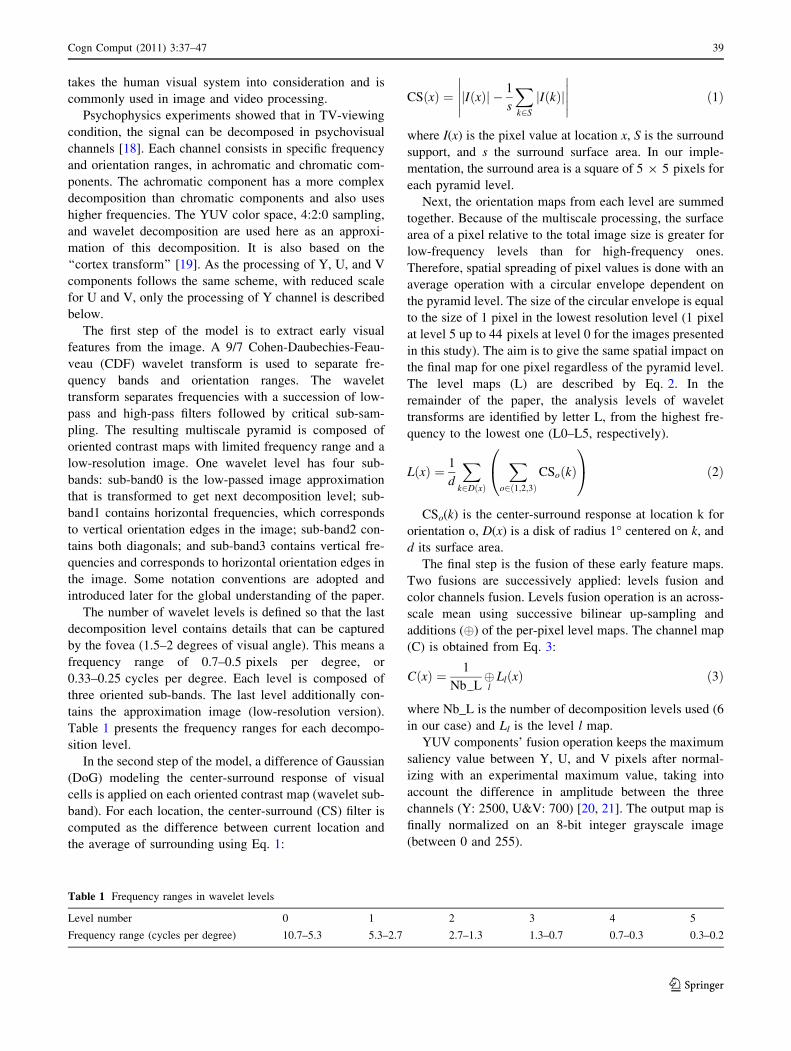
takes the human visual system into consideration and is

commonly used in image and video processing.

Psychophysics experiments showed that in TV-viewing

condition, the signal can be decomposed in psychovisual

channels [18]. Each channel consists in specific frequency

and orientation ranges, in achromatic and chromatic com-

ponents. The achromatic component has a more complex

decomposition than chromatic components and also uses

higher frequencies. The YUV color space, 4:2:0 sampling,

and wavelet decomposition are used here as an approxi-

mation of this decomposition. It is also based on the

‘‘cortex transform’’ [19]. As the processing of Y, U, and V

components follows the same scheme, with reduced scale

for U and V, only the processing of Y channel is described

below.

The first step of the model is to extract early visual

features from the image. A 9/7 Cohen-Daubechies-Feau-

veau (CDF) wavelet transform is used to separate fre-

quency bands and orientation ranges. The wavelet

transform separates frequencies with a succession of low-

pass and high-pass filters followed by critical sub-sam-

pling. The resulting multiscale pyramid is composed of

oriented contrast maps with limited frequency range and a

low-resolution image. One wavelet level has four sub-

bands: sub-band0 is the low-passed image approximation

that is transformed to get next decomposition level; sub-

band1 contains horizontal frequencies, which corresponds

to vertical orientation edges in the image; sub-band2 con-

tains both diagonals; and sub-band3 contains vertical fre-

quencies and corresponds to horizontal orientation edges in

the image. Some notation conventions are adopted and

introduced later for the global understanding of the paper.

The number of wavelet levels is defined so that the last

decomposition level contains details that can be captured

by the fovea (1.5–2 degrees of visual angle). This means a

frequency range of 0.7–0.5 pixels per degree, or

0.33–0.25 cycles per degree. Each level is composed of

three oriented sub-bands. The last level additionally con-

tains the approximation image (low-resolution version).

Table 1 presents the frequency ranges for each decompo-

sition level.

In the second step of the model, a difference of Gaussian

(DoG) modeling the center-surround response of visual

cells is applied on each oriented contrast map (wavelet sub-

band). For each location, the center-surround (CS) filter is

computed as the difference between current location and

the average of surrounding using Eq. 1:

CSðxÞ ¼ IðxÞj j � 1

s

X

k2S

IðkÞj j�����

����� ð1Þ

where I(x) is the pixel value at location x, S is the surround

support, and s the surround surface area. In our imple-

mentation, the surround area is a square of 5 9 5 pixels for

each pyramid level.

Next, the orientation maps from each level are summed

together. Because of the multiscale processing, the surface

area of a pixel relative to the total image size is greater for

low-frequency levels than for high-frequency ones.

Therefore, spatial spreading of pixel values is done with an

average operation with a circular envelope dependent on

the pyramid level. The size of the circular envelope is equal

to the size of 1 pixel in the lowest resolution level (1 pixel

at level 5 up to 44 pixels at level 0 for the images presented

in this study). The aim is to give the same spatial impact on

the final map for one pixel regardless of the pyramid level.

The level maps (L) are described by Eq. 2. In the

remainder of the paper, the analysis levels of wavelet

transforms are identified by letter L, from the highest fre-

quency to the lowest one (L0–L5, respectively).

LðxÞ ¼ 1

d

X

k2DðxÞ

X

o2ð1;2;3ÞCSoðkÞ

0@

1A ð2Þ

CSo(k) is the center-surround response at location k for

orientation o, D(x) is a disk of radius 1� centered on k, and

d its surface area.

The final step is the fusion of these early feature maps.

Two fusions are successively applied: levels fusion and

color channels fusion. Levels fusion operation is an across-

scale mean using successive bilinear up-sampling and

additions (�) of the per-pixel level maps. The channel map

(C) is obtained from Eq. 3:

CðxÞ ¼ 1

Nb L�l

LlðxÞ ð3Þ

where Nb_L is the number of decomposition levels used (6

in our case) and Ll is the level l map.

YUV components’ fusion operation keeps the maximum

saliency value between Y, U, and V pixels after normal-

izing with an experimental maximum value, taking into

account the difference in amplitude between the three

channels (Y: 2500, U&V: 700) [20, 21]. The output map is

finally normalized on an 8-bit integer grayscale image

(between 0 and 255).

Table 1 Frequency ranges in wavelet levels

Level number 0 1 2 3 4 5

Frequency range (cycles per degree) 10.7–5.3 5.3–2.7 2.7–1.3 1.3–0.7 0.7–0.3 0.3–0.2

Cogn Comput (2011) 3:37–47 39

123

Note that for all the different filters and processing at the

border of the image, an infinite extension with mirror is

applied. As a result, the model is not centered biased. This

consideration is of importance because of the known center

bias existing in experimental eye-tracking data [22].

For fair comparison with state-of-the-art models that are

center-biased, a number of pixel rows and column from the

input picture borders are excluded from the computation.

The size of the borders is rescaled in the pyramidal

decomposition to avoid a bias in low-resolution levels, i.e.,

the number of discarded pixels becomes null when a suf-

ficiently high decomposition level is reached.

Experiment Setup

Stimuli and Category

This experiment uses four different sets of images

belonging to four semantic categories. The stimuli are

outdoor color images. These images are grouped into four

different categories: Coast, Mountain, Street, and Open-

Country. Each category contains pictures of our environ-

ment. Using different categories is motivated by the

different conclusions seen in the literature when using

different image types [7, 10].

Reference Predefined Pictures

Stimuli selection process is based on a database proposed

by Torralba and Oliva [14]. This database is composed of

10 categories. In order to limit the total number of stimuli

in our experiment and still obtain representative categories,

only four of them are used here: Coast, Mountain, Street,

and OpenCountry. These categories are interesting because

their Fourier spectrums are significantly different from

each other as illustrated by Fig. 2. This figure shows

average spectral profiles and associated distribution

histograms. Distribution corresponds to the distance d from

the mean magnitude spectrum normalized by the standard

deviation of the category (dðsÞ ¼ 1n�m

Pn;m

sðn;mÞ�j

ASðn;mÞj AS = average spectrum). The spectral profiles,

which reveal invariant global layouts of the categories, are

very distinct from one category to another. Indeed, Coast

spectrum presents vertically stretched diamond showing

horizontally oriented gist [23], and OpenCountry provides

a more proportioned diamond which suggests more

equality (on average) in the proportion between horizontal

and vertical aspects. Mountain spectrum is isotropic and

underlines random aspect of Mountain shapes. Street

spectrum is very stretched especially in horizontal axis and

in vertical axis, which reveals rectilinear elements char-

acterizing scene with artificial surroundings.

The principle of our selection is to choose our stimuli in

order to select images that are close to these Fourier

spectrums. It involves a selection process of our own

database from Fourier magnitude spectrum distribution of

Torralba and Oliva’s categories.

Stimuli Pool Constitution

A first database is composed of 242 color pictures. Each

picture has a resolution of 800 9 600 pixels. Our catego-

ries contain 59 Coast pictures, 44 Street pictures, 61

Mountain, and 78 OpenCountry pictures. Note that these

images were selected to present a virgin landscape with

very few salient or incongruent objects. The goal is to

reduce a bias in gaze allocation due to the presence of locus

strongly attracting the gaze such as a bird in OpenCountry

and the sky or a cottage in Mountain. The only present

objects were constitutive and integrated in surroundings

such as a parked car in Street category for example.

Torralba and Oliva’s Coast, Street, OpenCountry, and

Mountain reference categories contain 360, 292, 410, and

Fig. 2 Representation of the

mean spectrum of the 4 used

reference Torralba and Oliva’s

categories with associated

distribution histogram. (Picture

Database on

http://people.csail.mit.edu/

torralba/code/spatialenvelope/)

40 Cogn Comput (2011) 3:37–47

123

374 images, respectively. Torralba and Oliva’s picture

database has allowed obtaining reference categorical signal

definition (Fourier spectrum central tendencies and mean

variability). These categorical attributes are then used to

proceed with a stimuli selection across our own database,

to obtain a homogeneous and representative database in

terms of Fourier spectrum. The selection consists in

keeping images having spectrums closer than one standard

deviation from the reference category. The distance mea-

sure used is the average Euclidean distance

(dðsÞ ¼ 1n�m

Pn;m

sðn;mÞ � ASðn;mÞj j AS = average spec-

trum). The selection process has rejected 47.5% on the total

of our database of initial stimuli. This selection ensures to

have an intracategorical homogeneity and representative-

ness, based on the selection criteria. The rationale is to use

typical features in order to keep general aspects of the

categories. The categories contain 30–34 remaining ima-

ges. Each of the four final categories is constituted of

exactly 30 pictures to have equal-sized categories.

Protocol

Forty voluntary participants (22 men and 18 women, mean age

= 36.7) of Technicolor Research and Innovation in Cesson-

Sevigne (France) participated in this experiment. All subjects

had a normal or corrected-to-normal vision. The results from 3

participants have been rejected because recording was

incomplete, resulting in a total of 37 observers.

Eye movements were recorded from an infrared reflec-

tion capture to detect pupil’s location using a SMI RED 50

IView X system with a 50-Hz sampling.

Stimuli were presented on a screen resolution of

1,280 9 972 pixels screen at a distance of 60 cm

(35� 9 27� of visual angle). Each subject recording began

with 9 calibration points. All stimuli were presented during

5,500 ms. The presentation order was randomized across

participants, and each stimulus was separated by a mid-

gray screen (30% on normalized scale). The subjects were

instructed to do natural free viewing of stimuli. Participants

were also informed that questions can be asked after the

presentation of a stimulus. The questions were only asked

in order to keep the subject concentrated on the stimuli.

The questions were randomized and were about global

content characteristics such as esthetic, chromatic, quality,

etc. in order to avoid a subject search strategy.

Data Processing

The scanpath composed of less than 5 fixations were

deleted because they reflect either missing recording or too

long fixations associated with visual fatigue. Next, to keep

only cognitively valid fixations corresponding to a

complete treatment and to reduce measure noise [24], the

fixation duration distribution of each scanpath was com-

puted to discard fixations outside the range [average

duration ±2 9 standard deviation]. This removed 5% of

fixations. After the filtering of fixations, each coordinate

was projected with a pixel periphery corresponding to 1.5�of visual angle (according to the experimental situation) to

obtain 4 9 30 eye-tracking fixation distribution maps from

a set of 37 subjects’ ocular fixations. Figure 3 shows two

examples of stimuli with superimposed fixations.

Results

As described in the previous section, an experimental

environment has been set up in order to record eye fixations

for four scene categories. A simple but efficient computa-

tional model of visual attention has also been proposed. In

this section, similarity between eye movements collected

on the image database and computational saliency maps is

investigated. It aims at measuring to what extent one fea-

ture at a given resolution may be more or less predictive of

attention than another.

This section is composed of two main parts. The pro-

posed model is first benchmarked and compared to existing

reference models. Then, attention prediction analysis is

performed using only selected features from the model.

More specifically, the relative impact of low, medium, and

high spatial frequencies on the prediction of attention is

examined. One particular interest of this analysis relies on

the use of four well-defined categories of outdoor visual

scenes.

To conduct this analysis, the degree of similarity

between the predicted saliency maps and the visual scan-

path is computed. Studies have shown that correlation

Fig. 3 Example of stimuli for the Street category (top left) and the

OpenCountry category (bottom left) with ocular fixation localizations

Cogn Comput (2011) 3:37–47 41

123

between fixation locations and signal features decreases in

function of the fixation number [4]. In order to measure

bottom-up attention only, or at least to limit top-down

effects, we use only the first five fixations of visual

scanpaths.

Several metrics can be used to assess the degree of

similarity between ground truth data and predicted sal-

iency. The normalized scanpath salience metric (NSS) [25]

has been chosen for its simplicity and its relevance. It has

the advantage to normalize the salience per scanpath:

scanpaths with different number of fixations have the same

weight. In other words, every observer has the same impact

on salience. Moreover, the NSS gives more weight to areas

more often fixated.

The NSS is the average value of the saliency map at

each fixation normalized per scanpath. First, the saliency

map is normalized to have zero mean and unit standard

deviation. Then, the per-fixation salience value is com-

puted as the average of the saliency map on the projection

of the fixation. A disk with a radius of 1.5� of visual angle

is used to project each fixation. Per-observer NSS is

computed as the average of per-fixation salience value

along the scanpath. The NSS is the average of the per-

observer NSS.

Performance of the Proposed Compared to Existing

Models

The proposed model is compared to four well-known

models of the literature. The first two are very simple non-

biologically plausible models: the centered and the random

model. The former consists of a centered bidimensional

Gaussian. It simply reflects that the center of the screen

attracts our gaze whatever the salience. This model is given

by the following equation, and an example is depicted in

Fig. 4 (fourth column):

SMcentred ¼ e�dðs; s0Þ

rc

where d(s, s0) is the Euclidean distance between s (the

current pixel) and s0 (the pixel at the center of the picture),

rc is the standard deviation of the Gaussian and represents

the spreading of the saliency distribution, and rc is set to

100 (5 times the number of pixels per degree).

The random model consists of splitting a predicted

saliency map into macroblocks of 16 9 16 pixels and

rearranging them randomly and spatially to recreate a

saliency map. An example is provided in Fig. 4 (third

column). Note that the random saliency map and the pre-

dicted saliency map have exactly the same distribution of

salience.

The last two models used in the comparison are the

well-known models of Itti and Koch [1] based on the

biologically plausible architecture of Koch and Ullman

[15], and the one of Bruce and Tsotsos [26] based on ICA

learning and information theory. These models are referred

to as Itti and Bruce, respectively. Note that these two

models are center-biased due to the handling of invalid

filter responses at the borders of images, as explained in

[27]. As a result, the saliency on the border of the image is

erased, as can be seen in Fig. 4. This phenomenon artifi-

cially improves the performance of the models because

experimental eye-tracking data are known to have a center

bias [22]. For a fair comparison, in addition to our pro-

posed model, we used a centered biased version of the

same model by discarding an 8-pixel-width border from the

input image (proposed ? bias). For the sake of comparison,

we also present the results associated with the proposed

model weighted by the same Gaussian as the centered

model (Proposed ? Centered).

Figure 5 gives the degree of similarity between different

models and human scanpaths in terms of NSS values.

Results are consistent with those previously published in

Fig. 4 Saliency maps for all evaluated models. Each row is the

results for a particular category. From top to bottom: Coast, Street,OpenCountry, and Mountain. From left to right, original picture,

human fixation distribution map, random map, centered map,

proposed saliency map, and Itti’s and Bruce’s saliency maps

42 Cogn Comput (2011) 3:37–47

123

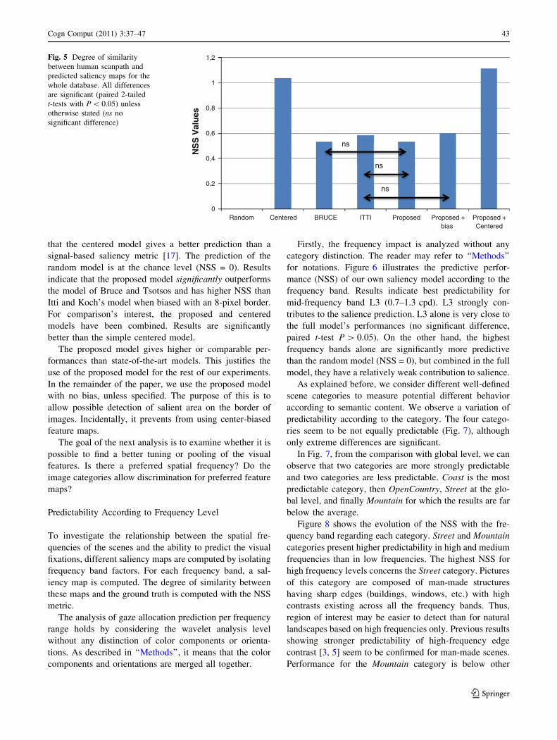
that the centered model gives a better prediction than a

signal-based saliency metric [17]. The prediction of the

random model is at the chance level (NSS = 0). Results

indicate that the proposed model significantly outperforms

the model of Bruce and Tsotsos and has higher NSS than

Itti and Koch’s model when biased with an 8-pixel border.

For comparison’s interest, the proposed and centered

models have been combined. Results are significantly

better than the simple centered model.

The proposed model gives higher or comparable per-

formances than state-of-the-art models. This justifies the

use of the proposed model for the rest of our experiments.

In the remainder of the paper, we use the proposed model

with no bias, unless specified. The purpose of this is to

allow possible detection of salient area on the border of

images. Incidentally, it prevents from using center-biased

feature maps.

The goal of the next analysis is to examine whether it is

possible to find a better tuning or pooling of the visual

features. Is there a preferred spatial frequency? Do the

image categories allow discrimination for preferred feature

maps?

Predictability According to Frequency Level

To investigate the relationship between the spatial fre-

quencies of the scenes and the ability to predict the visual

fixations, different saliency maps are computed by isolating

frequency band factors. For each frequency band, a sal-

iency map is computed. The degree of similarity between

these maps and the ground truth is computed with the NSS

metric.

The analysis of gaze allocation prediction per frequency

range holds by considering the wavelet analysis level

without any distinction of color components or orienta-

tions. As described in ‘‘Methods’’, it means that the color

components and orientations are merged all together.

Firstly, the frequency impact is analyzed without any

category distinction. The reader may refer to ‘‘Methods’’

for notations. Figure 6 illustrates the predictive perfor-

mance (NSS) of our own saliency model according to the

frequency band. Results indicate best predictability for

mid-frequency band L3 (0.7–1.3 cpd). L3 strongly con-

tributes to the salience prediction. L3 alone is very close to

the full model’s performances (no significant difference,

paired t-test P [ 0.05). On the other hand, the highest

frequency bands alone are significantly more predictive

than the random model (NSS = 0), but combined in the full

model, they have a relatively weak contribution to salience.

As explained before, we consider different well-defined

scene categories to measure potential different behavior

according to semantic content. We observe a variation of

predictability according to the category. The four catego-

ries seem to be not equally predictable (Fig. 7), although

only extreme differences are significant.

In Fig. 7, from the comparison with global level, we can

observe that two categories are more strongly predictable

and two categories are less predictable. Coast is the most

predictable category, then OpenCountry, Street at the glo-

bal level, and finally Mountain for which the results are far

below the average.

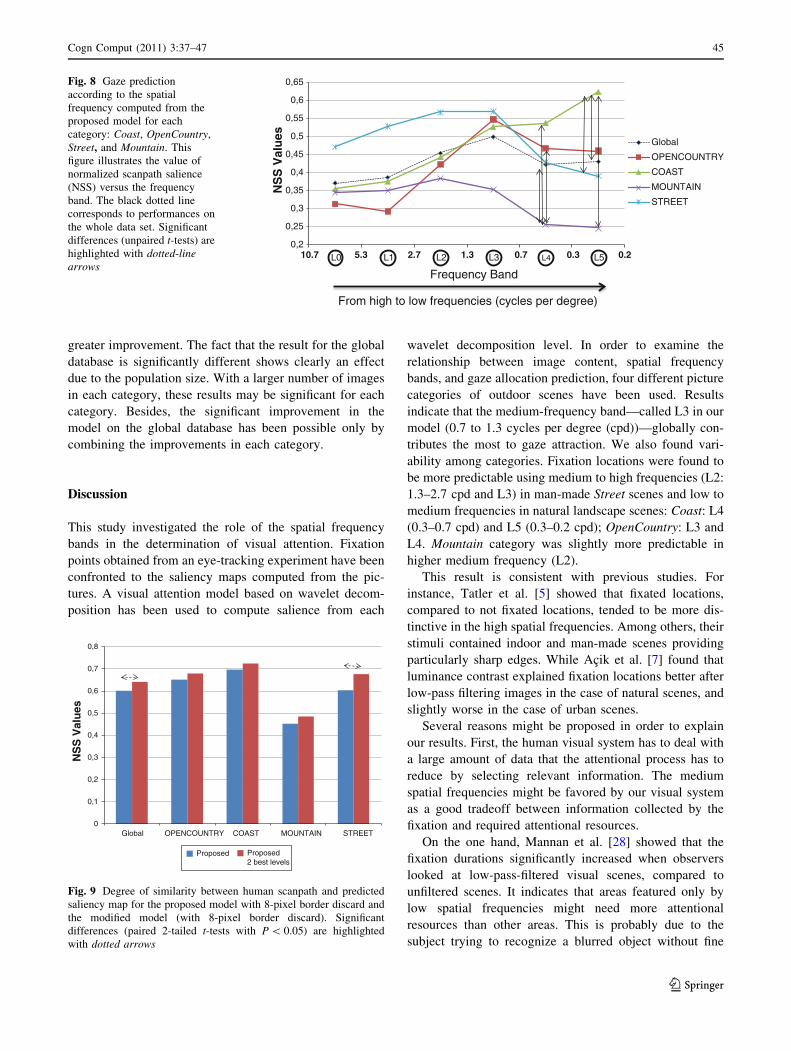
Figure 8 shows the evolution of the NSS with the fre-

quency band regarding each category. Street and Mountain

categories present higher predictability in high and medium

frequencies than in low frequencies. The highest NSS for

high frequency levels concerns the Street category. Pictures

of this category are composed of man-made structures

having sharp edges (buildings, windows, etc.) with high

contrasts existing across all the frequency bands. Thus,

region of interest may be easier to detect than for natural

landscapes based on high frequencies only. Previous results

showing stronger predictability of high-frequency edge

contrast [3, 5] seem to be confirmed for man-made scenes.

Performance for the Mountain category is below other

0

0,2

0,4

0,6

0,8

1

1,2

Random Centered BRUCE ITTI Proposed Proposed + bias

Proposed + Centered

NS

S V

alu

es

ns

ns

ns

Fig. 5 Degree of similarity

between human scanpath and

predicted saliency maps for the

whole database. All differences

are significant (paired 2-tailed

t-tests with P \ 0.05) unless

otherwise stated (ns no

significant difference)

Cogn Comput (2011) 3:37–47 43

123

categories (Fig. 7) and suggests that our model is not able

to reliably predict gaze allocation for this type of scene.

The curve obtained from Coast category shows a

monotonic increase in its NSS values with decreasing

spatial frequency. Low frequencies are thus stronger pre-

dictors of gaze allocation for this category.

The curve for OpenCountry clearly shows more

predictability in middle frequency (L3). Nevertheless, we

note that low-frequency bands (L4 and L5) perform better

than high-frequency bands (L0, L1, and L2). Prediction

performances for the frequency band L3 are almost the

same for three categories and correspond to the average

maximum.

Interestingly, per-frequency band NSS values are on

average better for Street than for OpenCountry, whereas

using the full model OpenCountry leads to the better per-

formance than Street. This could be due to frequency band

pooling that applies the same treatment to all frequency

bands. As natural images have a frequency power spectrum

biased toward low frequencies, more weight is given to

low-frequency features. Furthermore, in the case of Street

category, worse performances are obtained when pooling

all the frequency bands than when considering each fre-

quency band separately.

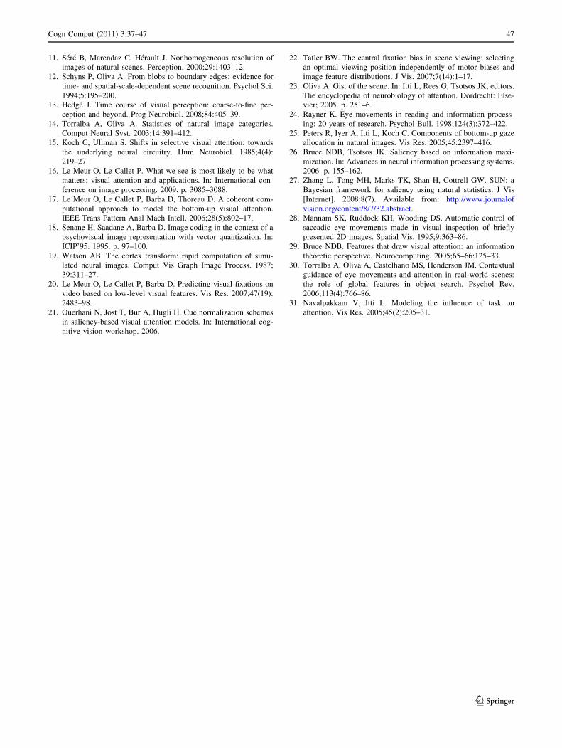
Model Improvement Based on Category Differentiation

Previous results indicate that there is a relationship

between salience, scene, and frequency band. Based on this

first conclusion, it seems possible to adjust the pooling of

the frequency bands in function of the scene type. For each

category, we use only the two best frequency levels (L3

and L4 for OpenCountry, L5 and L4 for Coast, L2 and L1

for Mountain, and L2 and L3 for Street) and the other

levels are discarded. Incidentally, the suppression of the

processing of some levels results in computational sim-

plification, especially at the largest resolution level L0 that

gives on average the worst performances and contains the

largest amount of data to process. Obtained results are

given in Fig. 9.

The modification of the model taking into account cat-

egory specificities improves the prediction performances

globally and for each category. The differences in results

are significant only for the global database and Street cat-

egory. Mountain, Coast, and OpenCountry present a sim-

ilar slight enhancement, but that was not found to be

significant. On the other hand, Street shows a significantly

Frequency Band

From high to low frequencies (cycles per degree)

0,2

0,25

0,3

0,35

0,4

0,45

0,5

0,55

L0 L1 L2 L3 L4 L5

NS

S V

alu

es

Full Proposed model

10.7 5.3 2.7 1.3 0.7 0.3 0.2

Fig. 6 Gaze prediction

according to the spatial

frequency for the whole

database. This figure illustrates

the value of normalized

scanpath salience (NSS) versus

the frequency bands for the

saliency computed from the

proposed model. All significant

paired t-tests (P \ 0.05) are

highlighted with dotted arrows.

Note that because there is a

dyadic resolution reduction

between pyramid levels, the

frequency axis is at a log scale

0

0,1

0,2

0,3

0,4

0,5

0,6

0,7

OPEN COUNTRY COAST MOUNTAIN STREET

Mea

n N

SS

val

ues

Global database average

Fig. 7 Gaze prediction according to the scene category (Mean NSS

per category). This figure illustrates attention prediction performances

according to the category. No difference is significant except

Mountain versus Coast (unpaired t-tests; P \ 0.05)

44 Cogn Comput (2011) 3:37–47

123

greater improvement. The fact that the result for the global

database is significantly different shows clearly an effect

due to the population size. With a larger number of images

in each category, these results may be significant for each

category. Besides, the significant improvement in the

model on the global database has been possible only by

combining the improvements in each category.

Discussion

This study investigated the role of the spatial frequency

bands in the determination of visual attention. Fixation

points obtained from an eye-tracking experiment have been

confronted to the saliency maps computed from the pic-

tures. A visual attention model based on wavelet decom-

position has been used to compute salience from each

wavelet decomposition level. In order to examine the

relationship between image content, spatial frequency

bands, and gaze allocation prediction, four different picture

categories of outdoor scenes have been used. Results

indicate that the medium-frequency band—called L3 in our

model (0.7 to 1.3 cycles per degree (cpd))—globally con-

tributes the most to gaze attraction. We also found vari-

ability among categories. Fixation locations were found to

be more predictable using medium to high frequencies (L2:

1.3–2.7 cpd and L3) in man-made Street scenes and low to

medium frequencies in natural landscape scenes: Coast: L4

(0.3–0.7 cpd) and L5 (0.3–0.2 cpd); OpenCountry: L3 and

L4. Mountain category was slightly more predictable in

higher medium frequency (L2).

This result is consistent with previous studies. For

instance, Tatler et al. [5] showed that fixated locations,

compared to not fixated locations, tended to be more dis-

tinctive in the high spatial frequencies. Among others, their

stimuli contained indoor and man-made scenes providing

particularly sharp edges. While Acik et al. [7] found that

luminance contrast explained fixation locations better after

low-pass filtering images in the case of natural scenes, and

slightly worse in the case of urban scenes.

Several reasons might be proposed in order to explain

our results. First, the human visual system has to deal with

a large amount of data that the attentional process has to

reduce by selecting relevant information. The medium

spatial frequencies might be favored by our visual system

as a good tradeoff between information collected by the

fixation and required attentional resources.

On the one hand, Mannan et al. [28] showed that the

fixation durations significantly increased when observers

looked at low-pass-filtered visual scenes, compared to

unfiltered scenes. It indicates that areas featured only by

low spatial frequencies might need more attentional

resources than other areas. This is probably due to the

subject trying to recognize a blurred object without fine

0,2

0,25

0,3

0,35

0,4

0,45

0,5

0,55

0,6

0,65

L0 L1 L2 L3 L4 L5

NS

S V

alu

es Global

OPENCOUNTRY

COAST

MOUNTAIN

STREET

Frequency Band

From high to low frequencies (cycles per degree)

10.7 5.3 2.7 1.3 0.7 0.3 0.2

Fig. 8 Gaze prediction

according to the spatial

frequency computed from the

proposed model for each

category: Coast, OpenCountry,

Street, and Mountain. This

figure illustrates the value of

normalized scanpath salience

(NSS) versus the frequency

band. The black dotted line

corresponds to performances on

the whole data set. Significant

differences (unpaired t-tests) are

highlighted with dotted-linearrows

0

0,1

0,2

0,3

0,4

0,5

0,6

0,7

0,8

Global OPENCOUNTRY COAST MOUNTAIN STREET

NS

S V

alu

es

Proposed Proposed2 best levels

Fig. 9 Degree of similarity between human scanpath and predicted

saliency map for the proposed model with 8-pixel border discard and

the modified model (with 8-pixel border discard). Significant

differences (paired 2-tailed t-tests with P \ 0.05) are highlighted

with dotted arrows

Cogn Comput (2011) 3:37–47 45

123

details. On the other hand, Fourier power spectrum in

natural scenes tends to fall with spatial frequency accord-

ing to a power law. It means that the scenes are composed

mostly of low and medium spatial frequencies, decreasing

information quality in high frequency. In order to optimize

the tradeoff between attentional resources and quality of

perception, it might be a good strategy to start our exam-

ination by the medium spatial frequencies. It does not mean

that the highest spatial frequencies are not useful. We can

make the assumption that in the case where the area under

inspection is interesting enough, our visual system can

switch toward a more accurate inspection, involving, this

time, a fine extraction based on the highest frequencies.

The second point concerns the task. In order to limit top-

down factors, observers in this study were instructed to

look freely the scene. Therefore, it might be that observers

do not pay attention to details, such as the texture of an

object. It would probably not be the case if a task was

given. For instance, a visual search of a target requires

much more attention than a free-view task, and presum-

ably, the detection scanning leads to a strategy involving

the processing of finest details provided by high frequen-

cies. In a task-viewing situation, the deployment of visual

attention may be more conscious and based on less-

redundant features such as high spatial frequencies in

accordance with the theory of information [29].

Therefore, we can suppose that medium frequencies

are globally more attractive in this study because they

constitute an ecological relevance and compromise

between attentional resources and information needed

when observers are not motivated by challenge of task

performing.

Tatler et al. [5] showed that local saliency of fixation

loci seems to be constant along the scanpath. They put

forward a strategic divergence model: top-down under-

standing may integrate information delivered by bottom-up

driving (saliency) to develop different strategies during

scene scanning to influence gaze driving. Saliency comes

from an integration of different feature channels and spatial

scales. Although saliency keeps its importance over time,

different feature channels and spatial scales may be useful

according to the different developed strategies along the

scanpath [7].

The difference in obtained results between the catego-

ries may thus result from an ecological determination of the

spatial scale to drive gaze allocation. Indeed, the medium-

frequency band L3 gives the best prediction in average.

Street category images are composed of objects such as

buildings, cars, and road signs that contain high-frequency

edges. The high-frequency driving of gaze allocation may

be due to the inspection of these objects. Natural Coast and

OpenCountry scenes have been selected to present very

few objects.

Even if high frequencies are present in Coast and

OpenCountry images, they are more related to landscape

texture such as rocks, forests, or grass constituting back-

ground than to object edges and do not attract the gaze.

Although it represents natural scenes, Mountain category

shows more predictability in high frequencies, but the

performance values are low. The saliency model may be

unable to model factors—or to integrate features—deter-

mining gaze driving in this category either because relevant

low-level features are missing or because top-down factors

may be more determinant for this category.

Finally, the fact that scene categories have distinct fre-

quency spectrums could bias frequency band preponder-

ance, because only available signal can drive fixations.

This could explain that the frequency band attracting most

the gaze varies in function of image category. However,

once integrating category-specific tuning in our saliency

model, the performances significantly improved. It means

that category-specific spectrums cannot explain alone the

role of the spatial frequency bands in the determination of

visual attention. This work can thus be used to improve

saliency models. A promising way to improve future

models would be to combine our approach with other

approaches using global semantic and context such as the

work of Torralba et al. [30]. The integration of top-down

factors, such as local object recognition [31], could also be

combined to our approach to improve saliency models.

References

1. Itti L, Koch C, Niebur E. Model of saliency-based visual attention

for rapid scene analysis. IEEE Trans Pattern Anal Mach Intell.

1998;20(11):1254–9.

2. Reinagel P, Zador AM. Natural scene statistics at the centre of

gaze. Comput Neural Syst. 1999;10:1–10.

3. Baddeley RJ, Tatler BW. High frequency edges (but not contrast)

predict where we fixate: a Bayesian system identification analy-

sis. Vis Res. 2006;46(18):2824–33.

4. Parkhurst D, Law K, Niebur E. Modeling the role of salience in

the allocation of overt visual attention. Vis Res. 2002;42:107–23.

5. Tatler BW, Baddeley RJ, Gilchrist ID. Visual correlates of fixa-

tion selection: effects of scale and time. Vis Res. 2005;45:643–59.

6. Bruce NDB, Loach DP, Tsotsos JK. Visual correlates of fixation

selection: a look at the spatial frequency domain. In: International

conference on image processing. 2007.

7. Acik A, Onat S, Schumann F, Einhauser W, Konig P. Effects of

luminance contrast and its modifications on fixation behavior

during free viewing of images from different categories. Vis Res.

2009;49(12):1541–53.

8. Billock VA. Neural acclimation to 1/f spatial frequency spectra in

natural images transduced by the human visual system. Phys D

Nonlinear Phenom. 2000;137(3–4):379–91.

9. Thorpe S, Fize D, Marlot C. Speed of processing in the human

visual system. Nature. 1996;381:520–2.

10. Mermillod M, Guyader N, Chauvin A. The coarse-to-fine

hypothesis revisited: evidence from neuro-computational mod-

eling. Brain Cogn. 2005;57(2):151–7.

46 Cogn Comput (2011) 3:37–47

123

11. Sere B, Marendaz C, Herault J. Nonhomogeneous resolution of

images of natural scenes. Perception. 2000;29:1403–12.

12. Schyns P, Oliva A. From blobs to boundary edges: evidence for

time- and spatial-scale-dependent scene recognition. Psychol Sci.

1994;5:195–200.

13. Hedge J. Time course of visual perception: coarse-to-fine per-

ception and beyond. Prog Neurobiol. 2008;84:405–39.

14. Torralba A, Oliva A. Statistics of natural image categories.

Comput Neural Syst. 2003;14:391–412.

15. Koch C, Ullman S. Shifts in selective visual attention: towards

the underlying neural circuitry. Hum Neurobiol. 1985;4(4):

219–27.

16. Le Meur O, Le Callet P. What we see is most likely to be what

matters: visual attention and applications. In: International con-

ference on image processing. 2009. p. 3085–3088.

17. Le Meur O, Le Callet P, Barba D, Thoreau D. A coherent com-

putational approach to model the bottom-up visual attention.

IEEE Trans Pattern Anal Mach Intell. 2006;28(5):802–17.

18. Senane H, Saadane A, Barba D. Image coding in the context of a

psychovisual image representation with vector quantization. In:

ICIP’95. 1995. p. 97–100.

19. Watson AB. The cortex transform: rapid computation of simu-

lated neural images. Comput Vis Graph Image Process. 1987;

39:311–27.

20. Le Meur O, Le Callet P, Barba D. Predicting visual fixations on

video based on low-level visual features. Vis Res. 2007;47(19):

2483–98.

21. Ouerhani N, Jost T, Bur A, Hugli H. Cue normalization schemes

in saliency-based visual attention models. In: International cog-

nitive vision workshop. 2006.

22. Tatler BW. The central fixation bias in scene viewing: selecting

an optimal viewing position independently of motor biases and

image feature distributions. J Vis. 2007;7(14):1–17.

23. Oliva A. Gist of the scene. In: Itti L, Rees G, Tsotsos JK, editors.

The encyclopedia of neurobiology of attention. Dordrecht: Else-

vier; 2005. p. 251–6.

24. Rayner K. Eye movements in reading and information process-

ing: 20 years of research. Psychol Bull. 1998;124(3):372–422.

25. Peters R, Iyer A, Itti L, Koch C. Components of bottom-up gaze

allocation in natural images. Vis Res. 2005;45:2397–416.

26. Bruce NDB, Tsotsos JK. Saliency based on information maxi-

mization. In: Advances in neural information processing systems.

2006. p. 155–162.

27. Zhang L, Tong MH, Marks TK, Shan H, Cottrell GW. SUN: a

Bayesian framework for saliency using natural statistics. J Vis

[Internet]. 2008;8(7). Available from: http://www.journalof

vision.org/content/8/7/32.abstract.

28. Mannam SK, Ruddock KH, Wooding DS. Automatic control of

saccadic eye movements made in visual inspection of briefly

presented 2D images. Spatial Vis. 1995;9:363–86.

29. Bruce NDB. Features that draw visual attention: an information

theoretic perspective. Neurocomputing. 2005;65–66:125–33.

30. Torralba A, Oliva A, Castelhano MS, Henderson JM. Contextual

guidance of eye movements and attention in real-world scenes:

the role of global features in object search. Psychol Rev.

2006;113(4):766–86.

31. Navalpakkam V, Itti L. Modeling the influence of task on

attention. Vis Res. 2005;45(2):205–31.

Cogn Comput (2011) 3:37–47 47

123