J.M. Lopez, J. Vega, S. Dormido-Canto, A. Murari, J.M. Ramirez,M. Ruiz, G. de Arcas and JET EFDA contributors

EFDA–JET–PR(12)59

Integration and Validation of a Disruption Predictor

Simulator in JET

“This document is intended for publication in the open literature. It is made available on the understanding that it may not be further circulated and extracts or references may not be published prior to publication of the original when applicable, or without the consent of the Publications Officer, EFDA, Culham Science Centre, Abingdon, Oxon, OX14 3DB, UK.”

“Enquiries about Copyright and reproduction should be addressed to the Publications Officer, EFDA, Culham Science Centre, Abingdon, Oxon, OX14 3DB, UK.”

The contents of this preprint and all other JET EFDA Preprints and Conference Papers are available to view online free at www.iop.org/Jet. This site has full search facilities and e-mail alert options. The diagrams contained within the PDFs on this site are hyperlinked from the year 1996 onwards.

Integration and Validation of a Disruption Predictor

Simulator in JET

J.M. Lopez1, J. Vega2, S. Dormido-Canto3, A. Murari4, J.M. Ramirez3,M. Ruiz1, G. de Arcas1 and JET EFDA contributors*

1CAEND. Universidad Politécnica de Madrid, Spain2Asociación EURATOM CIEMAT para Fusión Madrid, Spain

3Departamento Informática y Automática. UNED. Madrid, Spain4Consorzio RFX-Associazione EURATOM ENEA per la Fusione, Padova, Italy

* See annex of F. Romanelli et al, “Overview of JET Results”,(23rd IAEA Fusion Energy Conference, Daejon, Republic of Korea (2010)).

JET-EFDA, Culham Science Centre, OX14 3DB, Abingdon, UK

Preprint of Paper to be submitted for publication in Proceedings of the 7th Workshop on Fusion Data Processing Validation and Analysis, Frascati, Roma, Italy

26th March 2012 - 28th March 2012

.

1

ABSTRACTDisruptions in tokamak devices are inevitable and can severely damage the device’s wall [1, 2]. For this reason, different protection mechanisms have to be implemented. In Join European Torus (JET), these protection systems are structured in different levels. At the lowest level are those systems that are responsible for protecting the machine’s integrity, which must be highly reliable. More complex systems are located at higher levels; these higher-level systems have been designed to take action before low-level systems. Since the installation of the new metallic wall [3] in JET, new protection systems have been being developed to improve the overall protection of the device. This work focuses on a software application – a disruption predictor – that detects an incoming disruption. This software application simulates the behavior of a real-time implementation. In recent years, efforts have been devoted to developing and optimizing a reliable system that is capable of predicting disruptions. This has been accomplished by the novel combination of machine learning techniques based on supervised learning methods [4]. Disruptions must be predicted early enough so that the protection systems can mitigate the effects of disruptions. This article summarizes the software development of the JET disruption predictor. This software simulates the real-time data acquisition and data processing. It has been an essential software tool to both optimize the disruption prediction model and implement a simulator of the real-time predictor.

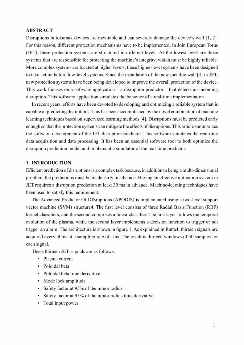
1. INTRODUCTIONEfficient prediction of disruptions is a complex task because, in addition to being a multi-dimensional problem, the predictions must be made early in advance. Having an effective mitigation system in JET requires a disruption prediction at least 30 ms in advance. Machine-learning techniques have been used to satisfy this requirement. The Advanced Predictor Of DISruptions (APODIS) is implemented using a two-level support vector machine (SVM) structure4. The first level consists of three Radial Basis Function (RBF) kernel classifiers, and the second comprises a linear classifier. The first layer follows the temporal evolution of the plasma, while the second layer implements a decision function to trigger or not trigger an alarm. The architecture is shown in figure 1. As explained in Ratta4, thirteen signals are acquired every 30ms at a sampling rate of 1ms. The result is thirteen windows of 30 samples for each signal. These thirteen JET- signals are as follows:

• Plasma current• Poloidal beta• Poloidal beta time derivative• Mode lock amplitude• Safety factor at 95% of the minor radius• Safety factor at 95% of the minor radius time derivative• Total input power

2

• Plasma internal inductance• Plasma internal inductance time derivative• Plasma vertical centroid position• Plasma density• Stored diamagnetic energy time derivative• Net power (total input power minus total radiated power)

A Discrete Fourier Transform (DFT) is performed on the 30 sample windows using a Fast Fourier Transform (FFT) algorithm to obtain a spectrum estimation and build a feature vector (1).

(1)

The vector components are the spectral deviations calculated using

(2)

where S refers to the mean value of the DFT coefficients Si[k] for k=1 to 15. The feature vectors XN are used to calculate the distances D1, D2 and D3 to the respective separating hyper-planes [5] of each first layer classifier using

(3)

in this equation, the αi, veci, γ and Bias are values obtained during the training process of the first layer classifiers. These distances are the inputs to the second layer classifier. This classifier implements a decision function (4).

(4)

the coefficients a and β are obtained during the training process of the decision function. In order to improve the results of the Ratta predictor [4], time domain information was included using the mean value. To allow the predictor to be used in real time, it is necessary to reduce the computational load. To this end, this work has been focused on reducing the number of signals used and optimizing the code execution time. To address this analysis, a trial-and-error procedure has been used to reduce the number of signals used. Three sets of signals, formed by 7, 8, and 12 signals, have produced optimal results. The windows have been resized to 32 points to achieve a shorter FFT computational time resulting from the use of a number of points that is a power of two [6].

XN = {σS0,... σS12}

σSx =|Si[k]|2

15Σ15k=1

DM = ( αi . e–γ||veci – XN ||2) – BiasΣN

i=1

R = (a3 . D3 + a2 . D2 + a1 . D1 + β

3

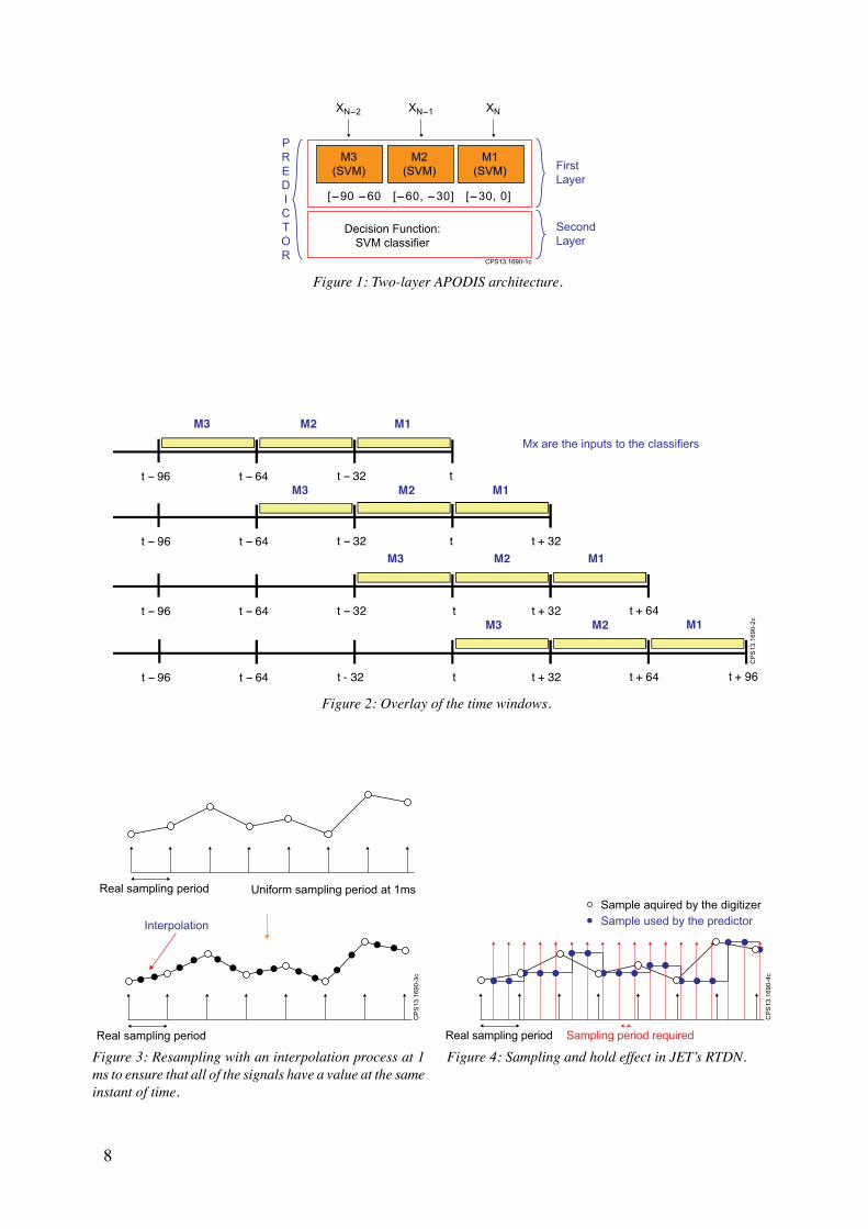
2. PREDICTOR ARCHITECTUREFigure 1 shows the two-layer architecture of APODIS. The input of the M1 classifier is the current feature vector X1 of the current data window from the current time to 32ms prior to the current time (t0 to t-32). The inputs of the M2 and M3 classifiers are the previous feature vectors from time t-32 to t-64 and t-64 to t-96, respectively. The inputs to the secondlayer classifier are the distances calculated in the M1, M2 and M3 classifiers. This classifier decides whether the alarm should be triggered. As shown in figure 2, there is an overlay due to the displacement of feature vectors in time.

3. TRAINING PROCESSThe predictor must be trained before it can be used. The training process is very important because it defines the model of the predictor, coefficients for the classifiers and the signals used. During the training process, two rates must be carefully assessed: the success rate and false alarm rate. Furthermore, the dataset that is chosen to perform the training is very important. A balanced dataset was chosen: 125 unintentional disruptive discharges and 100 non-disruptive ones. These discharges were randomly selected. The training datasets were obtained from JET campaigns C19, C20, C21 and C22. Campaigns C23, C24, C25, C26, C27a and C27b have been used for test purposes. Three sets of features with 14, 16 and 24 components (models A, B and C, respectively) were used as the input into the first layer. Table I shows the signals used. Before starting the training process, the signals have been preprocessed. The aforementioned signals have significantly different sampling period (non-homogeneous sampling period ranging from 10μs to 15ms). Thus, resampling was performed with a linear interpolation at 1ms. Following the resampling, all of the signals exist (have a value) at the same time instant. Figure 3 illustrates this process. Another potential issue is the amplitude difference between the signals, which can differ in several orders of magnitude. Therefore, a normalization process was applied during the training phase. This normalization adjusts the signal values to the interval between 0 and 1, preserving their relative magnitudes.

(5)

4. IMPLEMENTATIONThe initial objective was to implement a program in “C” code to run in JET, showing the results of predictions via an on-line display in the control room for session leader assessment, and to store the alarms and results in the JET database. The application should be based on software code and data structures with an APODIS description. The data structures define the behavior of the program.

Inputsignal – MinMax – MinNormalized signal =

4

The code is unique and changes in the data structures define its behavior. However, deploying an application in JET’s infrastructure is not trivial. The developed application can be used like a real-time behavior simulator and run in the JET Analysis Cluster (JAC). New applications must be developed under the MARTe framework [7]. Having an application that can simulate the real-time behavior of the predictor before a MARTe application is designed is very helpful. An important aspect of this application is executed in the JET Analysis Cluster (JAC), which takes the signals from the JET database simulating the behavior of the JET’s Real-Time Data network (RTDN). When an unavailable sample is requested from the RTDN, the RTDN provides the previous value [8]. This effect must be studied because it was omitted during the training phase and may have modified the predictor’s success rate. Figure 4 illustrates this effect, which can be analyzed by the proposed application. The system architecture is shown in figure 5. The config and SVM model files define the behaviorof the current predictor. The output file shows the results of the discharge analysed, and if the predictor is in debug mode, an execution trace is dumped to debug the files. All of the parameters that modify the behavior of the program are defined in a config file, which allows for the modification of various parameters:

• Plasma current threshold to start the predictor• Sampling period• Window size• Number of signals used• Number of signals to be derived from the raw signals• Number of window models• Path for files: maximums, minimums, and file model description

The signals to be read from the JET database are specified in an external file. The entire path name to the JET database must be used. If the signal to be read is not available in the real-time format, the name must be preceded by an asterisk (*) so that the signal is read for the processed database. Figure 6 shows a sample file, with the signal name for model A. To allow the user changing all of the configuration parameters, the application has been developed using dynamic data structures. Each input signal is loaded into an array of signal structures. Figure 7 shows the data structure used. The structure is self-contained, as it stores all of the information needed to handle the signal according to the program’s requirements. The signals’ raw data are stored in this original form using two dynamic buffer pointers with *pData and *pTime. The predictor’s architecture uses windows to follow the temporal evolution of the signal. These windows are handled by a dynamic array, and only one window is writing at a specific instant with the data sampling at 1ms. These windows are passed to the SVM classifiers using the movement of pointers to reduce the execution time. Note that only the resampling time information for the last window is stored. This information is needed

5

when a disruption is detected and an alarm is triggered. In this situation, the alarm time provided is the time value of the last sample in the time window. The program can be set to several debug modes. In these modes, the application saves internal information to files, allowing the execution of the program to be followed and the time evolution of the partial results of the classifier to be obtained. This information is very useful for tracing the program execution with the results of the training phase.

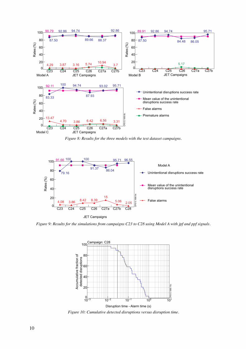
RESULTSFigure 8 shows the results for the three models in each campaign. Four values are represented:

• The unintentional disruption success rate, which is the main objective of the predictor.• The false alarm rate, which indicates that the predictor has triggered an alarm for a

nondisruptive discharge.• The premature alarm rate, in which an alarm is triggered more than one second early.• The mean value of the unintentional disruption success rate.

Table II summarizes the results related to the number of discharges tested. The number of disruptive discharges (unintentional) is 228, and the total number of safe discharges is 3578. In addition to optimizing the success rate, the predictor should minimize the number of false alarms. Model A achieves these objectives and uses the smallest number of signals, which is very important for a real-time implementation because it reduces the computation time. Thus, model A was chosen for further analysis using the simulator to obtain data for its future realtime implementation. Note that these results are with the carbon wall. The new metal wall was introduced into the C28 campaign and the discharges from 80128 to 81051. Some real-time systems were not working; therefore, the signals used in the training phase were not available. This was the case for the system BetaLi, which provides some signals for APODIS. Thus, to avoid the lack of realtime signals in the database, another method was used to employ processed signals and test the simulator with the new wall. Thus, the predictor was tested using three real-time signals and four processed signals: plasma internal inductance, plasma density, stored diamagnetic energy and total input power. With this new approach, a new simulation was performed for campaigns C23 to C27b and tested with the new data in C28 with a metal wall. Figure 9 presents these results. For campaign C28, 678 shots were analyzed from discharges 80128 to 81051: 633 of the discharges were safe, 33 were unintentional and 12 were intentional. Once the success and false alarm rates are within a reasonable range, it is important to know whether the predictions are made sufficiently in advance. Figure 10 presents the accumulative detected disruptions versus disruption time from the discharges analyzed in campaign C28. Using the criteria that 30ms is sufficient to take protective actions in JET, figure 10 shows that 90% of alarms are detected at least 30ms in advance. This result shows that the success rate of the predictor is lower; however, a success rate of 90% is still sufficient for the predictor to be considered viable.

6

CONCLUSIONSExcellent results were obtained by the disruption predictor simulation studied in this work. Three models with different numbers of signals were examined. The model with seven signals (model A) was shown to be the best option. This model has a success rate of 90.79%, which is 1.32% less than that of model C (the optimal model), and a false alarm rate of 5.11%. By using the minimum number of signals, the computation time is reduced. The developed simulator is a valuable tool; it has revealed that the sample and hold effects that appear in the RTDN when a sample is not available do not affect the predictor or degrade the predictor’s success rate. The results obtained with campaign C28 are very important, as they show that the predictor’s architecture is robust and that the success rate does not decrease when using the metal wall, despite the predictor having been trained with a carbon wall.

ACKNOWLEDGMENTSThis work was partially funded by the Spanish Ministry of Science and Innovation under Project Nos. ENE2008-02894/FTN and ENE2009-10280 and was carried out within the framework of the European Fusion Development Agreement. The views and opinions expressed herein do not necessarily reflect those of the European Commission.

REFERENCES[1]. A.H. Boozer, “Theory of tokamak disruptions.” Physics of plasmas, Vol 19, pp. 25, ( 2012).[2]. J. Pamela, G.F. Matthews, V. Philipps, R. Kamendje et al. “An ITER-like wall for JET”.

Journal of Nuclear Materials. Vol 363-365. pp 11. (2007).[3]. G.M. et al “JET ITER-like Wall- Overview and experimental programme”, Proceedings of

the 13th International Workshop on Plasma Facing Materials and Components for Fusion Applications, Rosenheim. Germany. (2011)

[4]. G.A. Ratta, J. Vega, A. Murari, G. Vagliasindi, M.F. Johnson, P.C. Vries et al. “An Advanced Disruption Predictor for JET tested in simulated Real time Environment”. Nuclear Fusion. vol. 50, pp 10. (2010)

[5]. V. Cherkassky and F. Mulier. “Learning from data” New York, Wiley (1998).[6]. M. Ruiz, J. Vega, G. Arcas, G. Ratta, E. Barrera, A. Murari, J.M. Lopez, R. Melendez,

“Realtime plasma disruptions detection in JET implemented with the ITMS platform using FPGA based IDAQ”. IEEE Transactions on Nuclear Science. Vol. 58, Issue: 4, Part:1. pp: 1576-1581. (2011)

[7]. A.C. Neto, F. Sartori, F. Piccolo, R. Vitelli, G. de Tommasi, L. Zabeo et al. “MARTe: a multiplatform real-time framework”. IEEE Transactions on Nuclear Science. vol. 57, n 2, pp. 479-486. (2010).

[8]. R. Felton, K. Blackler, S. Dorling, A. Goodyear, O. Hemming et al. “Real-time plasma control at JET using an ATM network”. Real Time Conference. Santa Fe. 11th IEEE NPSS. Pp 175-181. (1999).

7

Table I: Signals used in models tested. Grey values are calculated from the signals read from the JETs database.

Table II: Results obtained with the 3 models.

8

Figure 2: Overlay of the time windows.

Figure 3: Resampling with an interpolation process at 1 ms to ensure that all of the signals have a value at the sameinstant of time.

Figure 4: Sampling and hold effect in JET’s RTDN.Real sampling period

Interpolation

CP

S13

.169

0-3c

Real sampling period Uniform sampling period at 1ms

Real sampling period

Sample aquired by the digitizerSample used by the predictor

CP

S13

.169

0-4c

Sampling period required

Figure 1: Two-layer APODIS architecture.

Decision Function:SVM classifier

XN-2

[-90 -60 [-60, -30] [-30, 0]

PREDICTOR

M3(SVM)

XN-1 XN

FirstLayer

SecondLayer

CPS13.1690-1c

M2(SVM)

M1(SVM)

tt - 32t - 64t - 96

M1M2M3

t + 32tt - 32t - 64t - 96

M1M2M3

t + 64t + 32tt - 32t - 64t - 96

M1M2M3

t + 96t + 64t + 32tt - 32t - 64t - 96

M1M2M3

Mx are the inputs to the classifiers

CP

S13

.169

0-2c

9

Figure 5: Predictor system architecture. Figure 6: Signal list file.

Figure 7: Structure used to store the signal read from the JET database.

JET Analysis Cluster (JAC)

PREDICTOR

Sig

nal D

ata

Bas

e

ConfigFile

DDBB OutputFile

DebugOutput

SVMModel

CP

S13

.169

0-5c

CP

S13

.169

0-6c

Array Signals

CP

S13

.169

0-7c

10

Figure 10: Cumulative detected disruptions versus disruption time.

Figure 8: Results for the three models with the test dataset campaigns.

Figure 9: Results for the simulations from campaigns C23 to C28 using Model A with jpf and ppf signals.

80

60

40

20

0

100

10-2 10-1 10010-3 101

Acc

umul

ativ

e fra

ctio

n of

dete

cted

dis

rupt

ions

Disruption time - Alarm time (s)

CP

S13

.169

0-10

c

Campaign: C28

80

100

60

40

20

0C23 C24 C25 C26 C27a C27b

Rat

es (%

)

JET CampaignsModel C

CP

S13

.169

0-8c

80

100 90.79

87.50

89.91

87.50

92.86 94.74

84.48 86.05

95.71

5.17

92.86 94.74

89.66 88.37

10.943.75.743.163.87

92.86

60

40

20

0C23

4.29

13.474.70 3.86 6.42 6.56 3.31

83.33

100 94.74

87.93

93.02 95.7192.11

C24 C25 C26 C27a C27b

Rat

es (%

)

JET CampaignsModel A

80

100

60

40

20

0C23 C24 C25 C26 C27a C27b

Rat

es (%

)

JET CampaignsModel B

Unintentional disruptions success rate

Mean value of the unintentionaldisruptions success rate

False alarms

Premature alarms

80

100

60

40

20

0C23 C24 C25 C26 C27a C27b C28

Rat

es (%

)

JET Campaigns

Model A

CP

S13

.169

0-9c

Unintentional disruptions success rate

Mean value of the unintentionaldisruptions success rate

False alarms

91.66

79.16

100 100

91.37

95.71

86.04

96.55

4.08 3.86 8.42 8.3915

5.06 2.05