Interplay between charge, magnetic and superconducting ...

Interplay between charge, magnetic and superconductingproperties in copper-based and iron-based

superconductors

A DISSERTATION

SUBMITTED TO THE FACULTY OF THE GRADUATE SCHOOL

OF THE UNIVERSITY OF MINNESOTA

BY

Xiaoyu Wang

IN PARTIAL FULFILLMENT OF THE REQUIREMENTS

FOR THE DEGREE OF

Doctor of Philosophy

Prof. Rafael M. Fernandes

August, 2017

c© Xiaoyu Wang 2017

ALL RIGHTS RESERVED

Acknowledgements

In 2010, I graduated with a Bachelor’s degree in Electrical Engineering, decided to

follow my interest in theoretical physics, and came to the physics graduate program

in University of Minnesota. Upon completion of this thesis, my years in the graduate

school will come to a happy ending, and I am ready to start a new chapter as a physics

postdoctoral researcher in University of Chicago. Looking back, the seven years were

filled with obstacles and bitterness. However, these make the accomplishments all the

more valuable. I am thankful to all the people who have helped me achieving my goals in

research, as well as giving me the courage and perseverance to carry on amid difficulties.

First and foremost, I am deeply indebted to my adviser Prof. Rafael Fernandes, for

all the efforts he put into preparing me for a career in academia. He is very approachable

as an adviser, offering all the help I ever wanted when I got stuck in the middle of a

project. He is very active in referring me to various workshop opportunities which are of

enormous help to building my career. More importantly, his great passion for physics,

critical thinking, and rigorous attitude towards research all greatly benefitted me as a

person.

I am thankful to Prof. Alex Kamenev, who I worked with during my first three

years in graduate school, and still maintain excellent relationship. Although it is a bit

unfortunate that our collaborations hadn’t resulted in published works, I learned a good

deal from him on the methods of studying nonequilibrium phenomena.

I am also greatly thankful to Dr. Jian Kang, Dr. Yuxuan Wang, Dr. Yoni Schat-

tner, Dr. Michael Schutt, Dr. Peter Orth and Dr. Morten Christensen for valuable

discussions and collaborations in research.

I want to thank my friends for being part of my life during the seven years in

Minnesota, including Qianhui Shi, Tobias Gulden, Yangmu Li, Ruiqi Xing, Tianbai

i

Cui, Jiaming Zheng, Yang Tang, Qi Shao, Han Fu, Michael Albright, Yanqing Sun and

many others. I also want to acknowledge the Twin Cities Go Club and the U of M Go

Club, which kept me (happily) busy on the weekends.

Last but not least, I want to say thank you to my parents, who supported me through

16 years of school in China, and endured my seven years away from home in the United

States with only increasing love and patience.

I also acknowledge financial supports from teaching and research assistantships of-

fered by the School of Physics and Astronomy in University of Minnesota, the Hoff Lu

fellowship granted by Mike and Lester Lu, and the Doctoral Dissertation Fellowship of-

fered by the graduate school in University of Minnesota. In addition, I also acknowledge

funding granted by the Department of Energy.

ii

Dedication

This thesis is dedicated to my beloved parents, Jianjun Wang and Huimin Li.

iii

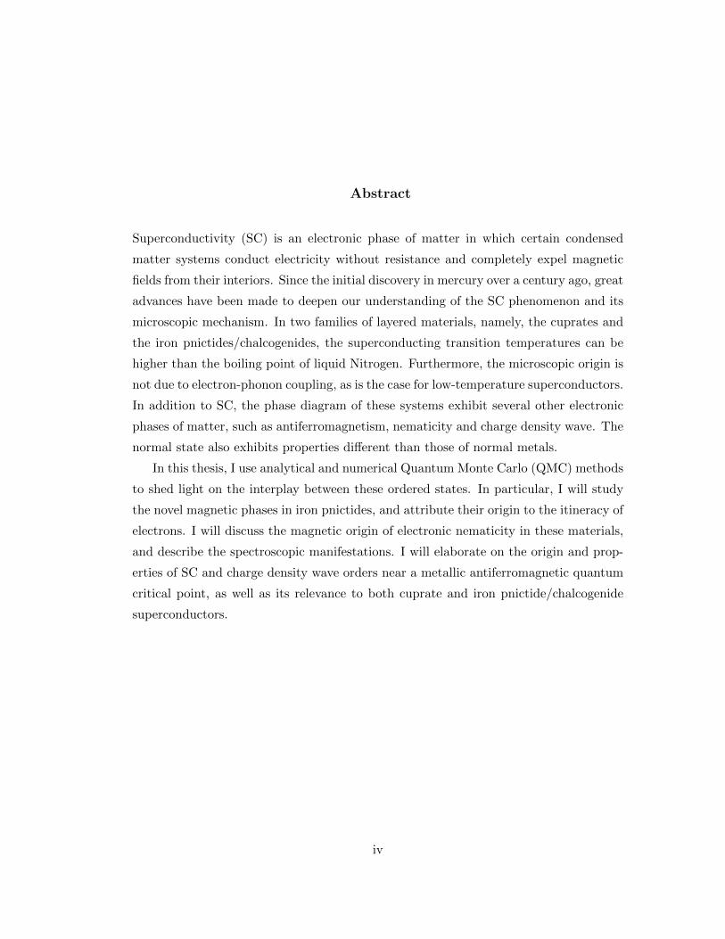
Abstract

Superconductivity (SC) is an electronic phase of matter in which certain condensed

matter systems conduct electricity without resistance and completely expel magnetic

fields from their interiors. Since the initial discovery in mercury over a century ago, great

advances have been made to deepen our understanding of the SC phenomenon and its

microscopic mechanism. In two families of layered materials, namely, the cuprates and

the iron pnictides/chalcogenides, the superconducting transition temperatures can be

higher than the boiling point of liquid Nitrogen. Furthermore, the microscopic origin is

not due to electron-phonon coupling, as is the case for low-temperature superconductors.

In addition to SC, the phase diagram of these systems exhibit several other electronic

phases of matter, such as antiferromagnetism, nematicity and charge density wave. The

normal state also exhibits properties different than those of normal metals.

In this thesis, I use analytical and numerical Quantum Monte Carlo (QMC) methods

to shed light on the interplay between these ordered states. In particular, I will study

the novel magnetic phases in iron pnictides, and attribute their origin to the itineracy of

electrons. I will discuss the magnetic origin of electronic nematicity in these materials,

and describe the spectroscopic manifestations. I will elaborate on the origin and prop-

erties of SC and charge density wave orders near a metallic antiferromagnetic quantum

critical point, as well as its relevance to both cuprate and iron pnictide/chalcogenide

superconductors.

iv

Contents

Acknowledgements i

Dedication iii

Abstract iv

List of Figures viii

1 Introduction 1

1.1 Superconductivity . . . . . . . . . . . . . . . . . . . . . . . . . . . . . . 1

1.2 Structural properties . . . . . . . . . . . . . . . . . . . . . . . . . . . . . 4

1.3 Electronic phase diagram . . . . . . . . . . . . . . . . . . . . . . . . . . 5

1.4 Electronic properties and theoretical modeling . . . . . . . . . . . . . . . 7

1.5 Quantum criticality . . . . . . . . . . . . . . . . . . . . . . . . . . . . . . 9

1.6 Overview . . . . . . . . . . . . . . . . . . . . . . . . . . . . . . . . . . . 10

2 Magnetism in iron-based superconductors 12

2.1 Introduction . . . . . . . . . . . . . . . . . . . . . . . . . . . . . . . . . . 12

2.2 Ginzburg-Landau analysis . . . . . . . . . . . . . . . . . . . . . . . . . . 17

2.3 Microscopic origin for magnetism . . . . . . . . . . . . . . . . . . . . . . 19

2.3.1 Multi-orbital Hubbard model for iron pnictide materials . . . . . 20

2.3.2 Localized J1-J2 Heisenberg model . . . . . . . . . . . . . . . . . 20

2.3.3 Itinerant picture and the three band model . . . . . . . . . . . . 21

2.3.4 Away from perfect nesting . . . . . . . . . . . . . . . . . . . . . . 26

2.3.5 Neel antiferromagnetic fluctuations . . . . . . . . . . . . . . . . . 30

v

2.4 Experimental manifestations of C4 magnetism . . . . . . . . . . . . . . . 33

2.4.1 Fermi surface reconstruction . . . . . . . . . . . . . . . . . . . . 33

2.4.2 Spin wave . . . . . . . . . . . . . . . . . . . . . . . . . . . . . . . 36

2.5 Conclusions . . . . . . . . . . . . . . . . . . . . . . . . . . . . . . . . . . 48

3 Origin of electronic nematicity in iron-based superconductors and man-

ifestations in Scanning Tunneling Spectroscopy 50

3.1 Introduction . . . . . . . . . . . . . . . . . . . . . . . . . . . . . . . . . . 50

3.2 Nematicity as a vestigial order to stripe magnetism . . . . . . . . . . . . 53

3.3 Spectroscopic manifestations of electronic nematic order driven by mag-

netic fluctuations . . . . . . . . . . . . . . . . . . . . . . . . . . . . . . . 56

3.3.1 Experimental results . . . . . . . . . . . . . . . . . . . . . . . . . 58

3.3.2 Theoretical analysis . . . . . . . . . . . . . . . . . . . . . . . . . 60

3.4 Conclusions . . . . . . . . . . . . . . . . . . . . . . . . . . . . . . . . . . 67

4 Antiferromagnetic quantum criticality and numerical solutions of the

spin-fermion model 69

4.1 Introduction . . . . . . . . . . . . . . . . . . . . . . . . . . . . . . . . . . 69

4.2 The spin-fermion model . . . . . . . . . . . . . . . . . . . . . . . . . . . 71

4.2.1 Eliashberg approach and superconductivity . . . . . . . . . . . . 73

4.2.2 Weak coupling and away from magnetic QCP . . . . . . . . . . . 75

4.2.3 Near the magnetic QCP: the importance of hot spots . . . . . . 76

4.2.4 Charge density wave and SU(2) symmetry . . . . . . . . . . . . . 82

4.2.5 Summary of results . . . . . . . . . . . . . . . . . . . . . . . . . . 83

4.3 Determinantal Quantum Monte Carlo and applications to the spin-fermion

model . . . . . . . . . . . . . . . . . . . . . . . . . . . . . . . . . . . . . 84

4.3.1 Introduction . . . . . . . . . . . . . . . . . . . . . . . . . . . . . 84

4.3.2 DQMC procedure for the two-band spin-fermion model . . . . . 85

4.3.3 Summary . . . . . . . . . . . . . . . . . . . . . . . . . . . . . . . 86

4.4 Superconductivity mediated by quantum critical antiferromagnetic fluc-

tuations: the rise and fall of hot spots . . . . . . . . . . . . . . . . . . . 87

4.4.1 Introduction . . . . . . . . . . . . . . . . . . . . . . . . . . . . . 87

4.4.2 Electronic band dispersion . . . . . . . . . . . . . . . . . . . . . . 87

vi

4.4.3 DQMC procedure . . . . . . . . . . . . . . . . . . . . . . . . . . 89

4.4.4 Tc dependence on hot spot properties . . . . . . . . . . . . . . . 93

4.4.5 Beyond hot spot: Tc at larger spin-fermion coupling . . . . . . . 96

4.4.6 Analysis and conclusion . . . . . . . . . . . . . . . . . . . . . . . 98

4.5 Interplay between superconductivity and charge density wave physics

near an antiferromagnetic quantum phase transition . . . . . . . . . . . 100

4.5.1 Introduction . . . . . . . . . . . . . . . . . . . . . . . . . . . . . 100

4.5.2 One-dimensional band dispersion . . . . . . . . . . . . . . . . . . 102

4.5.3 Half filling and exact SU(2) symmetry . . . . . . . . . . . . . . . 102

4.5.4 Main results from DQMC . . . . . . . . . . . . . . . . . . . . . . 106

4.5.5 Analysis and conclusion . . . . . . . . . . . . . . . . . . . . . . . 111

4.6 Conclusions . . . . . . . . . . . . . . . . . . . . . . . . . . . . . . . . . . 112

5 Conclusion 114

Appendix A. Determinantal Quantum Monte Carlo and Application to

two band spin-fermion model 116

A.1 Monte Carlo basics . . . . . . . . . . . . . . . . . . . . . . . . . . . . . . 116

A.2 Applications to coupled boson-fermion system . . . . . . . . . . . . . . . 118

A.3 Computing fermionic Green’s function . . . . . . . . . . . . . . . . . . . 119

A.4 Monte Carlo procedure . . . . . . . . . . . . . . . . . . . . . . . . . . . . 120

A.5 Fermion sign problem . . . . . . . . . . . . . . . . . . . . . . . . . . . . 122

A.6 Sign-problem free DQMC for two-band spin-fermion model . . . . . . . 123

A.7 XY spin and simplification of the fermionic Hamiltonian . . . . . . . . . 124

A.8 Reducing finite size effects using a magnetic flux . . . . . . . . . . . . . 125

References 128

vii

List of Figures

1.1 Superconductors discovered over the years . . . . . . . . . . . . . . . . . 2

1.2 Crystal structure of cuprate materials . . . . . . . . . . . . . . . . . . . 3

1.3 Crystal structure of iron pnictide and chalcogenide materials . . . . . . 4

1.4 Electronic phase diagram of cuprate materials . . . . . . . . . . . . . . . 5

1.5 Electronic phase diagram of iron pnictide and chalcogenide materials . . 7

1.6 Schematic phase diagram near a quantum critical point . . . . . . . . . 10

2.1 Tetragonal magnetic phase in iron pnictide materials . . . . . . . . . . . 13

2.2 Inelastic neutron scattering results on Ba(Fe1−xCox)2As2 . . . . . . . . 14

2.3 Three types of magnetic orders in iron pnictide materials . . . . . . . . 15

2.4 Mean field phase diagram of the Ginzburg-Landau free energy . . . . . . 19

2.5 Fermi surface of iron pnictide materials and an effective three-band de-

scription . . . . . . . . . . . . . . . . . . . . . . . . . . . . . . . . . . . . 22

2.6 Doping dependence of the quartic Ginzburg-Landau coefficients u and g 27

2.7 Feynman diagrams containing the leading-order corrections to the free

energy arising from the residual U7 interaction . . . . . . . . . . . . . . 28

2.8 Magnetic phase diagram of Ba(Fe1−xMnx)2As2 and measurements from

inelastic neutron scattering . . . . . . . . . . . . . . . . . . . . . . . . . 31

2.9 Feynman diagrams associated with the coupling between the Neel anti-

ferromagnetic fluctuations and the magnetic order parameters . . . . . . 32

2.10 Fermi surface reconstruction due to stripe and CSDW magnetic orders . 35

2.11 Magnetic unit cell of stripe and SVC magnetic orders . . . . . . . . . . 37

2.12 Spin wave dispersions in the stripe magnetic state . . . . . . . . . . . . 40

2.13 Spin wave dispersions in the SVC state . . . . . . . . . . . . . . . . . . . 43

2.14 Spin-spin structure factor calculated for the stripe magnetic order . . . 45

viii

2.15 Spin-spin structure factor calculated for the SVC order . . . . . . . . . . 47

3.1 Schematic phase diagram of iron pnictide superconductors . . . . . . . . 51

3.2 Magnetic scenario for nematicity in the iron pnictide materials . . . . . 52

3.3 Nature of the nematic phase transition in the magnetic scenario . . . . . 56

3.4 Phase diagram of NaFe1−xCoxAs . . . . . . . . . . . . . . . . . . . . . . 58

3.5 LDOS and QPI patterns in the stripe magnetic phase . . . . . . . . . . 59

3.6 LDOS and QPI patterns in the nematic phase . . . . . . . . . . . . . . . 60

3.7 Temperature evolution of the anisotropy parameter . . . . . . . . . . . . 61

3.8 Fermi surface of our effective four band model . . . . . . . . . . . . . . . 63

3.9 Theoretically calculated QPI in the normal state, nematic and magnetic

phase . . . . . . . . . . . . . . . . . . . . . . . . . . . . . . . . . . . . . 66

4.1 Schematic band dispersion and Fermi surface based ARPES measure-

ments of optimally doped Bi2Sr2CuO6+x . . . . . . . . . . . . . . . . . . 72

4.2 Feynman diagrams considered in the Eliashberg approach . . . . . . . . 74

4.3 Fermi surface and hot spot pairs . . . . . . . . . . . . . . . . . . . . . . 76

4.4 Fermi surfaces corresponding to the two bands in the first Brillouin zone,

for different values of δ/t . . . . . . . . . . . . . . . . . . . . . . . . . . . 89

4.5 Binder cumulant B and static spin susceptibility χM as a function of r

for various temperatures . . . . . . . . . . . . . . . . . . . . . . . . . . . 90

4.6 Frequency and momentum dependence of the magnetic propagator ex-

tracted from QMC . . . . . . . . . . . . . . . . . . . . . . . . . . . . . . 91

4.7 Static pairing susceptibility χpair in the sign-changing gap channel and

in the in the sign-preserving gap channel as function of the distance to

the QCP at r = rc . . . . . . . . . . . . . . . . . . . . . . . . . . . . . . 93

4.8 Superfluid density ρs(L, T ) as function of temperature T for the band

dispersion δ/t = 0.6 and coupling constant λ2 = 8t for various system

sizes L . . . . . . . . . . . . . . . . . . . . . . . . . . . . . . . . . . . . . 94

4.9 The QMC extracted Tc (L) as function of the inverse system size 1/L for

all band dispersion parameters δ/t . . . . . . . . . . . . . . . . . . . . . 95

4.10 The superconducting transition temperature Tc at the QCP for different

band dispersion parameters . . . . . . . . . . . . . . . . . . . . . . . . . 96

ix

4.11 Universal temperature dependence of the pairing susceptibility χpair at

the QCP . . . . . . . . . . . . . . . . . . . . . . . . . . . . . . . . . . . . 97

4.12 Dependence of the superconducting transition temperature on the inter-

action strength . . . . . . . . . . . . . . . . . . . . . . . . . . . . . . . . 98

4.13 Purely one dimensional Fermi surface used in our studies . . . . . . . . 103

4.14 Non-interacting charge susceptibility in the Brillouin zone . . . . . . . . 104

4.15 Charge and superconducting susceptibilities in the momentum space at

the magnetic QCP . . . . . . . . . . . . . . . . . . . . . . . . . . . . . . 107

4.16 d-wave charge (left) and superconducting (right) susceptibilities plotted

versus distance to magnetic QCP for temperatures β = 6, 10, 16. . . . . 108

4.17 Superfluid density versus temperature for L = 8, 10, 12, and the extracted

BKT transition temperature Tc(L) . . . . . . . . . . . . . . . . . . . . . 109

4.18 Charge susceptibilities in the momentum space for period-125 , period-3,

period-4 and period-6 charge density wave orders. All results are obtained

at the magnetic QCP. β = 12. . . . . . . . . . . . . . . . . . . . . . . . . 109

4.19 Charge and superconducting susceptibilities of various band dispersions

for a inverse fixed temperature β = 12 . . . . . . . . . . . . . . . . . . . 110

4.20 Inverse charge and superconducting susceptibilities versus temperature

at the magnetic QCP. . . . . . . . . . . . . . . . . . . . . . . . . . . . . 111

4.21 Charge susceptibilities in the magnetically ordered phase versus at the

magnetic quantum critical point . . . . . . . . . . . . . . . . . . . . . . 111

A.1 Finite size effects on the compressibility of the non-interacting electronic

system, calculated from the density-density correlation function . . . . . 126

x

Chapter 1

Introduction

1.1 Superconductivity

In condensed matter systems, one of the most fascinating phenomena is the emergence of

various electronic phases of matter due to the interactions between individual electrons.

Such phases of matter exhibit collective properties, with collective excitations different

than that of a single electron. Among the many electronic phases is superconductiv-

ity, where the system conducts electricity without resistance, and expels magnetic field

completely from its interior. Such electric and magnetic properties make superconduc-

tors useful for many applications, such as dissipationless power transmission, magnetic

sensing, and quantum computation.

Superconductivity was first discovered in 1911 in mercury below a critical tem-

perature of 4.2K. The past century saw great advances in our understanding of the

phenomenon, as well as the discovery and synthesis of new superconducting materi-

als. Fig. 1.1 is a summary of the families of superconducting materials as well as their

transition temperatures. There are metallic elements such as mercury and lead, metal-

lic alloys such as niobium nitride and magnetism diboride, heavy fermion compounds

such as UPt3, fullerene compounds such as Cs3C60, and organic compounds such as

carbon nanotubes. In addition, there are the copper-oxide (cuprate) and the iron-

pnictide/chalcogenide superconductors discovered in 1986 and 2008 respectively. They

are also called high Tc superconductors and unconventional superconductors, because

the transition temperature surpasses the boiling point of liquid nitrogen (77K), and the

1

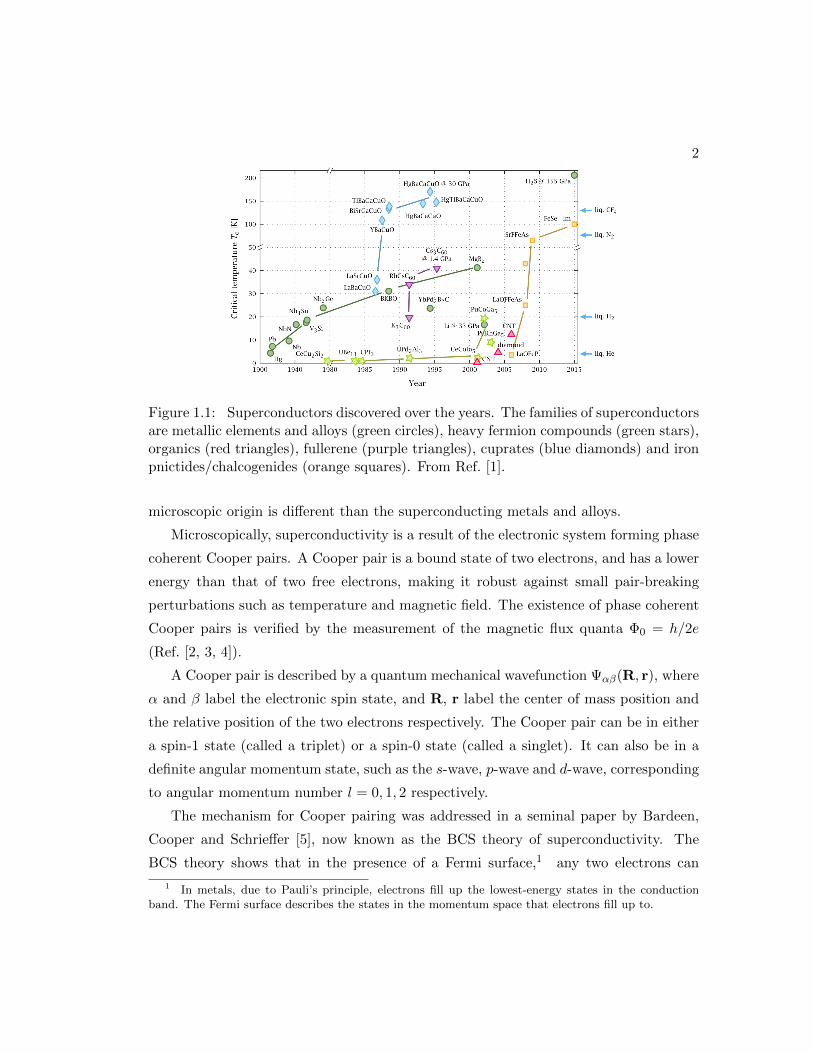
2

Figure 1.1: Superconductors discovered over the years. The families of superconductorsare metallic elements and alloys (green circles), heavy fermion compounds (green stars),organics (red triangles), fullerene (purple triangles), cuprates (blue diamonds) and ironpnictides/chalcogenides (orange squares). From Ref. [1].

microscopic origin is different than the superconducting metals and alloys.

Microscopically, superconductivity is a result of the electronic system forming phase

coherent Cooper pairs. A Cooper pair is a bound state of two electrons, and has a lower

energy than that of two free electrons, making it robust against small pair-breaking

perturbations such as temperature and magnetic field. The existence of phase coherent

Cooper pairs is verified by the measurement of the magnetic flux quanta Φ0 = h/2e

(Ref. [2, 3, 4]).

A Cooper pair is described by a quantum mechanical wavefunction Ψαβ(R, r), where

α and β label the electronic spin state, and R, r label the center of mass position and

the relative position of the two electrons respectively. The Cooper pair can be in either

a spin-1 state (called a triplet) or a spin-0 state (called a singlet). It can also be in a

definite angular momentum state, such as the s-wave, p-wave and d-wave, corresponding

to angular momentum number l = 0, 1, 2 respectively.

The mechanism for Cooper pairing was addressed in a seminal paper by Bardeen,

Cooper and Schrieffer [5], now known as the BCS theory of superconductivity. The

BCS theory shows that in the presence of a Fermi surface,1 any two electrons can

1 In metals, due to Pauli’s principle, electrons fill up the lowest-energy states in the conductionband. The Fermi surface describes the states in the momentum space that electrons fill up to.

3

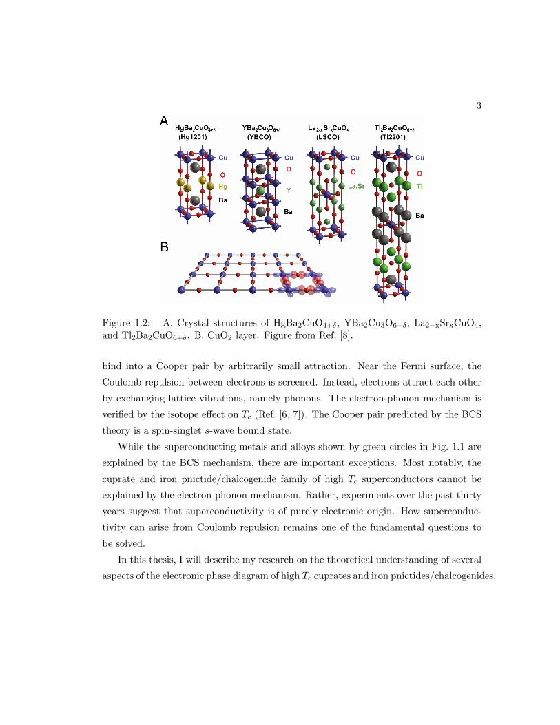
Figure 1.2: A. Crystal structures of HgBa2CuO4+δ, YBa2Cu3O6+δ, La2−xSrxCuO4,and Tl2Ba2CuO6+δ. B. CuO2 layer. Figure from Ref. [8].

bind into a Cooper pair by arbitrarily small attraction. Near the Fermi surface, the

Coulomb repulsion between electrons is screened. Instead, electrons attract each other

by exchanging lattice vibrations, namely phonons. The electron-phonon mechanism is

verified by the isotope effect on Tc (Ref. [6, 7]). The Cooper pair predicted by the BCS

theory is a spin-singlet s-wave bound state.

While the superconducting metals and alloys shown by green circles in Fig. 1.1 are

explained by the BCS mechanism, there are important exceptions. Most notably, the

cuprate and iron pnictide/chalcogenide family of high Tc superconductors cannot be

explained by the electron-phonon mechanism. Rather, experiments over the past thirty

years suggest that superconductivity is of purely electronic origin. How superconduc-

tivity can arise from Coulomb repulsion remains one of the fundamental questions to

be solved.

In this thesis, I will describe my research on the theoretical understanding of several

aspects of the electronic phase diagram of high Tc cuprates and iron pnictides/chalcogenides.

4

NATURE PHYSICS DOI: 10.1038/NPHYS1759 REVIEW ARTICLE

Box 1 |The iron-based superconductor family.

Iron, one of the most common metals on earth, has been knownas a useful element since the aptly named Iron Age. However,it was not until recently that, when combined with elementsfrom the group 15 and 16 columns of the periodic table (named,respectively, the pnictogens, after the Greek verb for choking,and chalcogens, meaning ‘ore formers’), iron-based metals wereshown to readily harbour a new form of high-temperature su-perconductivity. This general family of materials has quicklygrown to be large in size, with well over 50 different compoundsidentified that show a superconducting transition that occursat temperatures approaching 60K, and includes a plethora ofdifferent variations of iron- and nickel-based systems. So far, fiveunique crystallographic structures have been shown to supportsuperconductivity. As shown in Fig. B1a, these structures allpossess tetragonal symmetry at room temperature and rangefrom the simplest ↵-PbO-type binary element structure to morecomplicated quinternary structures composed of elements thatspan the entire periodic table.

The key ingredient is a quasi-two-dimensional layer consistingof a square lattice of iron atoms with tetrahedrally coordinatedbonds to either phosphorus, arsenic, selenium or tellurium anionsthat are staggered above and below the iron lattice to form achequerboard pattern that doubles the unit-cell size, as shownin Fig. B1b. These slabs are either simply stacked together, as inFeSe, or are separated by spacer layers using alkali (for example,Li), alkaline-earth (for example, Ba), rare-earth oxide/fluoride(for example, LaO or SrF) or more complicated perovskite-typecombinations (for example, Sr3Sc2O5). These so-called blockinglayers provide a quasi-two-dimensional character to the crystal

because they form atomic bonds of more ionic character with theFeAs layer, whereas the FeAs-type layer itself is held together bya combination of covalent (that is, Fe–As) and metallic (that is,Fe–Fe) bonding.

In the iron-basedmaterials, the commonFeAs building block isconsidered a critical component to stabilizing superconductivity.Because of the combination of strong bonding between Fe–Feand Fe–As sites (and even interlayer As–As in the 122-typesystems), the geometry of the FeAs4 tetrahedra plays a crucial rolein determining the electronic and magnetic properties of thesesystems. For instance, the two As–Fe–As tetrahedral bond anglesseem to play a crucial role in optimizing the superconductingtransition temperature (see the main text), with the highest Tcvalues found only when this geometry is closest to the ideal valueof 109.47.

Long-range magnetic order also shares a similar patternin all of the FeAs-based superconducting systems. As shownin the projection of the square lattice in Fig. B1b, the ironsublattice undergoes magnetic ordering with an arrangementconsisting of spins ferromagnetically arranged along onechain of nearest neighbours within the iron lattice plane,and antiferromagnetically arranged along the other direc-tion. This is shown on a tetragonal lattice in the figure,but actually only occurs after these systems undergo anorthorhombic distortion as explained in the main text. Inthe orthorhombic state, the distance between iron atoms withferromagnetically aligned nearest-neighbour spins (highlightedin Fig. B1b) shortens by approximately 1% as compared with theperpendicular direction.

FeSe

LiFeAsSrFe2As2

Sr3Sc2O5Fe2As2

LaFeAsO/SrFeAsF

a b

Figure B1 | Crystallographic and magnetic structures of the iron-based superconductors. a, The five tetragonal structures known to supportsuperconductivity. b, The active planar iron layer common to all superconducting compounds, with iron ions shown in red and pnictogen/chalcogenanions shown in gold. The dashed line indicates the size of the unit cell of the FeAs-type slab, which includes two iron atoms owing to the staggeredanion positions, and the ordered spin arrangement for FeAs-based materials is indicated by arrows (that is, not shown for FeTe).

of structural parameters, disorder location, chemical bonding anddensity. This is one of the key properties that has led to arapid but in-depth understanding of these materials. In due time,controlled experimental comparisons — for instance of Hall effect

(carrier density) under pressure versus doping, of different chemicalsubstitution series and further understanding of the local nature ofchemical substitution — will help pinpoint the important tuningparameters for these systems.

NATURE PHYSICS | VOL 6 | SEPTEMBER 2010 | www.nature.com/naturephysics 647

Figure 1.3: Crystal structures of FeSe, LiFeAs, BaFe2As2, and LaOFeAs. Fe atomsare colored red, and pnictogen/chalcogen atoms green. Taken from Ref. [9].

1.2 Structural properties

All cuprate high Tc superconductors have a layered structure as depicted in Fig. 1.2.

Some of the most studied materials include HgBa2CuO4+δ and YBa2Cu3O6+δ. All

cuprates have a stoichiometric CuO2 layer, where the copper atoms form a two dimen-

sional square lattice, with oxygen atoms residing on the centers of the bonds. The

CuO2 layer is believed to be responsible for the various low energy electronic proper-

ties. Additionally, there are spacer layers made of oxides (e.g., HgO) and cations (e.g.,

Y3+). Different families of cuprates have different numbers and contents of spacer layers.

These differences are responsible for the variations in the electronic phase diagram.

Like the cuprates, the iron pnictides/chalcogenides also have layered crystal struc-

tures, with a common layer made of iron pnictogen (e.g., FeAs) or iron chalcogen (e.g.,

FeSe). The Fe atoms form a square lattice. However, the pnictogens/chalcogens pro-

trude out of the two dimensional plane, forming a “puckering” pattern. The most stud-

ied families of compounds are the 11 family (e.g. FeSe/Te), the 111 family (NaFeAs),

the 1111 family (LaOFeAs), and the 122 family (BaFe2As2). Fig. 1.3 shows their crystal

structures.

5

x ¼ 0, CeCoIn5 becomes superconducting at temperaturesbelow approximately 2.3 K. Then as the Cd concentrationincreases, one enters a region where the system first becomesantiferromagnetic and then below the superconducting Tc

there is a coexistence regime. Finally, for Cd concentrationx * 0:15, superconductivity is absent and the Neel tempera-ture TN continues to increase. A similar phase diagram for thecase in which Co is replaced by Ir is shown in Fig. 6(b). In thiscase, while the Neel temperatures are comparable to thoseof the Co material, the superconducting Tc is significantlysmaller.

Figure 7 shows the phase diagrams of La2"xSrxCuO4 andNd2"xCexCuO4 (Armitage, Fournier, and Green, 2010).Undoped La2CuO4 and Nd2CuO4 are charge-transfer insula-tors which undergo antiferromagnetic Neel transitions as thetemperature drops below 300 K. Replacing a small amount ofLa with Sr leads to a hole doping of the CuO2 layer, whilereplacing Nd with Ce leads to an electron-doped CuO2 layer.

As the hole doping x increases, the Neel temperature issuppressed and at low temperatures the system passes througha spin glass phase in which local charge and spin orderedregions may be pinned. In the hole-doped case, the doping foroptimal superconductivity is well separated from the onset ofantiferromagnetism. The antiferromagnetic order extendsmuch farther out for the electron-doped system and appearsadjacent to the superconducting phase.

The phase diagram for one of the Fe-based superconduc-tors (Fernandes et al., 2010) BaðFe1"xCoxÞAs2 is shown inFig. 8. The parent compound BaFe2As2 is metallic and under-goes a structural tetragonal to orthorhombic transition and atthe same temperature an antiferromagnetic SDW transition.In the SDW phase the moments are oriented antiferro-magnetically along the longer a0 axis of the orthorhombic2Fe/cell and ferromagnetically along the b0 axis giving astripelike structure. As Co is added, the system is electrondoped and the structural and SDW transitions are suppressed.The structural transition is found to occur at temperaturesslightly above the SDW transition. For dopings x * 0:07, thestructural and SDW transitions are completely suppressedand the system goes into a superconducting state below Tc.However, for a range of smaller dopings 0:03 & x & 0:06 thesystem enters a region in which there is microscopic coex-istence of superconductivity, SDW, and orthorhombic order.As will be discussed, evidence for this is seen in the tem-perature dependence of the SDW Bragg peak intensity andthe orthorhombic distortion. It is also possible to hole dopethis compound (Rotter et al., 2008) by substituting K for Ba,Ba1"xKxFe2As2. Here again, as x increases the structural andSDW transition are suppressed and superconductivity onsets(Paglione and Greene, 2010).

C. Coexistence and interplay of antiferromagnetism andsuperconductivity

NMR as well as neutron scattering measurements hasprovided evidence that the observed coexistence regions insome systems represent microscopic coexistence in whichthe same electrons are involved with both the superconduc-tivity and the antiferromagnetism. For example, elasticneutron scattering measurements (Pham et al., 2006) onCeCoðIn0:9Cd0:1Þ5 find the integrated magnetic intensity atthe antiferromagnetic wave vector QAF versus temperatureshown in Fig. 9(a). This intensity is a measure of the square ofthe ordered magnetic moment and onsets at the Neel tem-perature TN . As seen in Fig. 9(a),M2ðTÞ initially increases asT decreases below TN , but then as T drops below the super-conducting transition temperature Tc, it saturates. Similardata for BaðFe1"xCoxÞAs2 at three different dopings areshown in Fig. 9(b). In this case, below Tc the ordered momentis reduced as the superconducting order increases. Both theseexamples reflect the competition of superconductivity andantiferromagnetism (Vorontsov, Vavilov, and Chubukov,2009; Fernandes et al., 2010). This competition is alsobelieved to be responsible for the anomalous suppression ofthe orthorhombic distortion in BaðFe1"xCoxÞAs2 as thetemperature decreases below Tc (Nandi et al., 2010).Evidence for atomic scale coexistence of superconductivityand antiferromagnetism for BaðFe1"xCoxÞ2As2 with x ¼ 0:06

FIG. 8 (color online). The phase diagram for BaðFe1"xCoxÞAs2.There appears a coexistence region similar to CeCoðIn1"xCdxÞ5shown in Fig. 6. From Fernandes et al., 2010.

FIG. 7 (color online). Schematic phase diagrams for hole-dopedLa2"xSrxCuO4 and electron-doped RE2"xCexCuO4 (RE ¼ La, Pr,Nd) cuprates (adapted from R. L. Greene and Kui Jin). In theelectron-doped case, the AF region extends to the superconductingregion, while in the hole-doped case a pseudogap region intervenes.

D. J. Scalapino: A common thread: The pairing interaction for . . . 1387

Rev. Mod. Phys., Vol. 84, No. 4, October–December 2012

Figure 1.4: Electronic phase diagram of both hole (right panel) and electron (left panel)doped cuprate superconductors. Taken from Ref. [10]. The parent compound is an an-tiferromagnetic Mott insulator. Superconductivity is achieved by electron/hole doping.In the hole-doped materials, there is a “pseudogap” phenomenon in the intermediatetemperature and doping ranges, characterized by suppressed electronic spectral weightat the Fermi surface. Near optimal doping, the disordered phase behaves like “strange”metal characterized by linear resistivity ρ ∝ T . The overdoped side is characterizedby standard Fermi liquid behavior. In recent years, various symmetry breakings havebeen observed inside the pseudogap region, including time reversal symmetry breaking,rotational symmetry breaking, and translational symmetry breaking.

1.3 Electronic phase diagram

Fig. 1.4 shows a typical electronic phase diagram of cuprates as a function of tempera-

ture and doping. The stoichiometric compounds are Mott insulators,2 which develop

antiferromagnetic order below a critical temperature. The antiferromagnetic order is

the Neel order, where the electronic spins on neighboring Cu atoms are antiparallel to

each other.

Superconductivity is achieved by doping charge carriers (electrons or holes) into the

CuO2 plane. This is done either by substituting the spacer layer cations by elements

in other columns of the periodic table, such as La2−xSrxCuO4, or by oxygen vacancies,

such as YBa2Cu3O6+δ. The antiferromagnetic order is suppressed as doping increases.

In addition to antiferromagnetism and superconductivity, the materials also exhibit

2 Mott insulators are metallic systems driven to an insulating phase due to strong electronicinteractions.

6

a ”pseudogap” region at intermediate temperature and doping ranges, characterized by

a loss of electronic spectral weight at the Fermi level.3 The pseudogap shows up in vari-

ous measures, including angle resolved photo-emission spectroscopy (ARPES), scanning

tunneling spectroscopy (STS), unform spin susceptibility, nuclear magnetic resonance

(NMR) and so on. It is unclear if the pseudogap temperature (T ∗) marks a true phase

transition or a crossover. Nonetheless, there have been reports on various symmetry

breaking phases occurring in the pseudogap region. Most notably, in recent years, static

charge density wave orders have been discovered in various cuprate materials, although

short-ranged in many cases[11, 12].

Another very interesting feature observed in both electron and hole-doped cuprates

is that near optimal doping (i.e., where superconducting Tc is highest), the normal

state exhibits strange metallic behaviors. Normal metals are described by the Landau

Fermi liquid theory, with electrical resistivity ρ ∝ T 2 due to quasiparticle scattering

from Coulomb interaction. However, the strange metallic phase is characterized by a

linear resistivity: ρ ∝ T . There are many proposals for the linear resistivity behavior,

including proximity to a quantum critical point[13, 14, 15], percolative transport[16]

etc. I will discuss quantum critical behaviors later in detail.

Fig. 1.5 shows the phase diagram of the iron pnictide material Ba(Fe1−xCox)2As2

and the iron chalcogenide material FeSe1−xSx. Both parent compounds (x = 0) are

metallic rather than insulating. In Ba(Fe1−xCox)2As2, the parent compound develops

a stripe-type magnetic order at low temperatures, where the spins in the Fe plane are

antiferromagnetically aligned along one Fe-Fe bond direction, and ferromagnetically

aligned along the other. The stripe magnetic order is preempted by a structural phase

transition, where the square lattice symmetry is broken down to orthorhombic. Such a

structural phase transition is also called a nematic phase transition. Superconductivity

is induced by doping, when both structural and magnetic phase transitions are sup-

pressed. In some iron pnictide materials, the normal state above optimal doping also

exhibits strange metal behavior[19].

In FeSe1−xSx, Se is substituted by S, of the same group in the periodic table. There-

fore, instead of doping charge carriers into the system, it is believed that the main effect

is to change the “chemical pressure”. The parent compound has a structural phase

3 Whether pseudogap phenomenon occurs in electron-doped materials is controversial.

7

x ¼ 0, CeCoIn5 becomes superconducting at temperaturesbelow approximately 2.3 K. Then as the Cd concentrationincreases, one enters a region where the system first becomesantiferromagnetic and then below the superconducting Tc

there is a coexistence regime. Finally, for Cd concentrationx * 0:15, superconductivity is absent and the Neel tempera-ture TN continues to increase. A similar phase diagram for thecase in which Co is replaced by Ir is shown in Fig. 6(b). In thiscase, while the Neel temperatures are comparable to thoseof the Co material, the superconducting Tc is significantlysmaller.

Figure 7 shows the phase diagrams of La2"xSrxCuO4 andNd2"xCexCuO4 (Armitage, Fournier, and Green, 2010).Undoped La2CuO4 and Nd2CuO4 are charge-transfer insula-tors which undergo antiferromagnetic Neel transitions as thetemperature drops below 300 K. Replacing a small amount ofLa with Sr leads to a hole doping of the CuO2 layer, whilereplacing Nd with Ce leads to an electron-doped CuO2 layer.

As the hole doping x increases, the Neel temperature issuppressed and at low temperatures the system passes througha spin glass phase in which local charge and spin orderedregions may be pinned. In the hole-doped case, the doping foroptimal superconductivity is well separated from the onset ofantiferromagnetism. The antiferromagnetic order extendsmuch farther out for the electron-doped system and appearsadjacent to the superconducting phase.

The phase diagram for one of the Fe-based superconduc-tors (Fernandes et al., 2010) BaðFe1"xCoxÞAs2 is shown inFig. 8. The parent compound BaFe2As2 is metallic and under-goes a structural tetragonal to orthorhombic transition and atthe same temperature an antiferromagnetic SDW transition.In the SDW phase the moments are oriented antiferro-magnetically along the longer a0 axis of the orthorhombic2Fe/cell and ferromagnetically along the b0 axis giving astripelike structure. As Co is added, the system is electrondoped and the structural and SDW transitions are suppressed.The structural transition is found to occur at temperaturesslightly above the SDW transition. For dopings x * 0:07, thestructural and SDW transitions are completely suppressedand the system goes into a superconducting state below Tc.However, for a range of smaller dopings 0:03 & x & 0:06 thesystem enters a region in which there is microscopic coex-istence of superconductivity, SDW, and orthorhombic order.As will be discussed, evidence for this is seen in the tem-perature dependence of the SDW Bragg peak intensity andthe orthorhombic distortion. It is also possible to hole dopethis compound (Rotter et al., 2008) by substituting K for Ba,Ba1"xKxFe2As2. Here again, as x increases the structural andSDW transition are suppressed and superconductivity onsets(Paglione and Greene, 2010).

C. Coexistence and interplay of antiferromagnetism andsuperconductivity

NMR as well as neutron scattering measurements hasprovided evidence that the observed coexistence regions insome systems represent microscopic coexistence in whichthe same electrons are involved with both the superconduc-tivity and the antiferromagnetism. For example, elasticneutron scattering measurements (Pham et al., 2006) onCeCoðIn0:9Cd0:1Þ5 find the integrated magnetic intensity atthe antiferromagnetic wave vector QAF versus temperatureshown in Fig. 9(a). This intensity is a measure of the square ofthe ordered magnetic moment and onsets at the Neel tem-perature TN . As seen in Fig. 9(a),M2ðTÞ initially increases asT decreases below TN , but then as T drops below the super-conducting transition temperature Tc, it saturates. Similardata for BaðFe1"xCoxÞAs2 at three different dopings areshown in Fig. 9(b). In this case, below Tc the ordered momentis reduced as the superconducting order increases. Both theseexamples reflect the competition of superconductivity andantiferromagnetism (Vorontsov, Vavilov, and Chubukov,2009; Fernandes et al., 2010). This competition is alsobelieved to be responsible for the anomalous suppression ofthe orthorhombic distortion in BaðFe1"xCoxÞAs2 as thetemperature decreases below Tc (Nandi et al., 2010).Evidence for atomic scale coexistence of superconductivityand antiferromagnetism for BaðFe1"xCoxÞ2As2 with x ¼ 0:06

FIG. 8 (color online). The phase diagram for BaðFe1"xCoxÞAs2.There appears a coexistence region similar to CeCoðIn1"xCdxÞ5shown in Fig. 6. From Fernandes et al., 2010.

FIG. 7 (color online). Schematic phase diagrams for hole-dopedLa2"xSrxCuO4 and electron-doped RE2"xCexCuO4 (RE ¼ La, Pr,Nd) cuprates (adapted from R. L. Greene and Kui Jin). In theelectron-doped case, the AF region extends to the superconductingregion, while in the hole-doped case a pseudogap region intervenes.

D. J. Scalapino: A common thread: The pairing interaction for . . . 1387

Rev. Mod. Phys., Vol. 84, No. 4, October–December 2012Figure 1.5: Electronic phase diagram of Ba(Fe1−xCox)2As2 (left panel) and FeSe1−xSx

(right panel), taken from Ref. [17] and Ref. [18] respectively. In Ba(Fe1−xCox)2As2, theparent compound is metallic, and develops a stripe-type antiferromagnetic magnetic or-der (AFM) at low temperatures. The stripe magnetic order is preempted by a structuralphase transition, where the square lattice symmetry is broken down to orthorhombic(Ort). Superconductivity (SC) is induced by doping, upon suppression of both struc-tural and magnetic phase transitions. In FeSe1−xSx, superconductivity exists even inthe parent compound, and persists when Se is substituted by S of the same group inthe periodic table. A structural phase transition (OO) occurs at a higher temperature.Unlike Ba(Fe1−xCox)2As2, there is no long range magnetic order.

transition (labeled by OO) occurring at about 90K. Unlike Ba(Fe1−xCox)2As2, there is

no long range magnetic order.4 In addition, the parent compound also exhibits a finite

superconducting transition temperature. Upon doping, the structural phase transition

is suppressed, and goes away near 15% of S substitution.

1.4 Electronic properties and theoretical modeling

The low energy electronic properties of both cuprates and iron pnictides/chalcogenides

are governed by the 3d electronic orbitals. There are five d electronic orbitals: dz2

(lz = 0), dxz/yz (lz = ±1), and dxy/x2−y2 (lz = ±2). The copper ion is in the Cu2+

valence state, with 3d9 electronic configuration. The iron ion is also in the 2+ valence

state, however with 3d6 electronic configuration.

In a free space, the five 3d orbitals have the same energy. The energy levels are split

4 Despite no long range magnetic order, there is experimental evidence for enhanced magneticfluctuations upon lowering temperature[20].

8

in a crystalline environment. In particular, in the cuprate materials, Cu2+ sits at the

center of a square of oxygen atoms.5 Crystal field splits the orbital degeneracy, with

dx2−y2 orbital having the highest energy. As a result, at low temperatures, four of the

five d orbitals are filled, while dx2−y2 orbital has only one electron, and is half filled.

On the other hand, in iron pnictide/chalcogenide materials, due to the “puckering” of

the pnictogen/chalcogen atoms, the crystal environment for an iron atom is between a

square and a tetrahedron. While a square environment makes the iron dz2/x2−y2 orbitals

(also called the eg orbitals) more energetic, a tetrahedron environment raises the energy

of the dxz/yz/xy (t2g) orbitals. The net result is that the crystal field splitting is much

smaller compared to that in the cuprates. Therefore, a low-energy description should

incorporate all five electronic orbitals[21].

Theoretically, one of the most studied microscopic models to describe these systems

is the Hubbard model. Hubbard models consist of two terms: a kinetic energy term

describing the electron hopping between sites, and a potential energy term describing

the screened Coulomb interactions, assumed to be onsite. The hopping amplitudes are

usually determined by tight-binding fits to density functional theory calculations.

A minimal model for the cuprates is the one-band Hubbard model, described as:

H =∑

ij,σ

(tij − µδij)c†iσcjσ + U∑

i

ni↑ni↓ (1.1)

where c†iσ creates an electron on site i with spin σ, t is the hopping amplitude be-

tween sites i and j, and U is the onsite Coulomb interaction. For the iron pnic-

tides/chalcogenides, one needs to study a multi-orbital Hubbard model [21], the details

of which will be presented later in Ch. 2.

The Hubbard models are microscopic models, and are usually very complicated to

solve beyond mean field approximation.6 Another theoretical approach to understand-

ing the electronic phase diagram is to construct low-energy effective field-theoretical

models. These models can usually be solved using well established methods, and can

offer great insights into the microscopic origin of various electronic phases.

5 Some cuprate compounds have apical oxygens as well, and the crystal field is of either elongatedoctahedral or square pyramidal type. dx2−y2 orbital still has the highest energy.

6 For a review of various analytical and numerical methods in solving Hubbard models, as wellas the various electronic phases emergent when electron density and Coulomb interaction strength aretuned, see Ref. [10].

9

1.5 Quantum criticality

In the cuprate phase diagram shown in Fig. 1.4, the transition temperature of the

antiferromagnetic order extrapolates to zero when doping is increased, suggesting a

“putative” antiferromagnetic quantum critical point (QCP).

A QCP marks a zero temperature continuous phase transition tuned by an exter-

nal parameter, such as doping, pressure, and disorder. In the cuprate and iron pnic-

tide/chalcogenide phase diagrams, various experiments have suggested the existence of

one or multiple “putative” QCPs, such as the antiferromagnetic QCP, the nematic QCP,

and the metal-insulator QCP. Interestingly, the optimal doping and the exotic normal

state properties are both achieved near one or more QCPs. This has motivated the

study of various low energy effective models describing electrons coupled to quantum

critical order parameter fluctuations[22, 23, 13, 14].

Similar to a continuous thermal phase transition, a QCP is characterized by a di-

vergent correlation length ξ → ∞ for the order parameter fluctuations. However, the

order parameter fluctuations near a QCP are different than near a thermal critical point,

in that its temporal fluctuations cannot be neglected. In particular, near a QCP, the

correlation time ξτ ∝ ξz also diverges, where z is called the dynamical critical exponent.

The quantum critical behavior of order parameter fluctuations extends to finite

temperatures, as shown in Fig. 1.6. This can be seen by comparing the timescales

associated with quantum decoherence7 τq and thermal equilibration τeq. The thermal

equilibration time is governed by temperature: τeq ∼ ~/kBT . The quantum decoherence

time diverges at QCP: τq ≡ ~/∆ ∼ ξτ , where ∆ is the corresponding energy scale. If τq >

τeq or ∆ < kBT , the thermal equilibration is faster than the quantum decoherence. As a

result, the order parameter fluctuations have slow dynamics, and temporal fluctuations

are important. On the other hand, if τq < τeq or ∆ > kBT , the quantum decoherence

happens faster than thermal equilibration. As a result, the order parameter fluctuations

can be treated thermally. As shown by Fig. 1.6, the crossover between quantum critical

fluctuations and thermal fluctuations is marked by a “fan” above the QCP.

In the studies using QCP as an organizing principle[22, 23, 13, 14], it is argued that

the coupling between quantum critical fluctuations and low energy electrons is key to

7 Quantum decoherence time is the timescale at which order parameter fluctuations are uncorrelated.See Ch.1 of Ref. [24]

10Quantum phase transitions 2075

r

T

rc0

thermallydisordered

quantumdisordered

quantum critical

ordered (at T = 0)

QCPrc

0

thermallydisordered

quantumdisordered

quantum critical

QCP

r

T

classicalcritical

ordered

(a) (b)non-universal non-universal

Figure 1. Schematic phase diagrams in the vicinity of a QCP. The horizontal axis representsthe control parameter r used to tune the system through the quantum phase transition, and thevertical axis is the temperature, T . (a) Order is only present at zero temperature. The dashedlines indicate the boundaries of the quantum critical region where the leading critical singularitiescan be observed; these crossover lines are given by kBT ∝ |r − rc|νz. (b) Order can also exist atfinite temperature. The solid line marks the finite-temperature boundary between the ordered anddisordered phases. Close to this line, the critical behaviour is classical.

fluctuations are important. It is located near the critical parameter value r = rc at comparativelyhigh (!) temperatures. Its boundaries are determined by the condition kBT > hωc ∝ |r −rc|νz:the system ‘looks critical’ with respect to the tuning parameter r , but is driven away fromcriticality by thermal fluctuations. Thus, the physics in the quantum critical region is controlledby the thermal excitations of the quantum critical ground state, whose main characteristic is theabsence of conventional quasiparticle-like excitations. This causes unusual finite-temperatureproperties in the quantum critical region, such as unconventional power laws, non-Fermiliquid behaviour, etc. Universal behaviour is only observable in the vicinity of the QCP, i.e.when the correlation length is much larger than microscopic length scales. Quantum criticalbehaviour is thus cut off at high temperatures when kBT exceeds characteristic microscopicenergy scales of the problem—in magnets this cutoff is, e.g., set by the typical exchangeenergy.

If order also exists at finite temperatures (figure 1(b)) the phase diagram is even richer.Here, a real phase transition is encountered upon variation of r at low T ; the QCP can beviewed as the endpoint of a line of finite-temperature transitions. As discussed earlier, classicalfluctuations will dominate in the vicinity of the finite-T phase boundary, but this region becomesnarrower with decreasing temperature, such that it might even be unobservable in a low-Texperiment. The fascinating quantum critical region is again at finite temperatures abovethe QCP.

A QCP can be generically approached in two different ways: r → rc at T = 0 or T → 0at r = rc. The power-law behaviour of physical observables in both cases can often be related.Let us discuss this idea by looking at the entropy, S. It goes to zero at the QCP (exceptions areimpurity transitions discussed in section 4), but its derivatives are singular. The specific heatC = T ∂S/∂T is expected to show power-law behaviour, as does the quantity B = ∂S/∂r .Using scaling arguments (see later), one can now analyse the ratio of the singular parts of B

and C: the scaling dimensions of T and S cancel, and therefore B/C scales as the inverse ofthe tuning parameter r . Thus, one obtains a universal divergence in the low-temperature limit,B/C ∝ |r − rc|−1; similarly, B/C ∝ T −1/νz at r = rc [17]. Note that B/C does not diverge ata finite-temperature phase transition. At a pressure-tuned phase transition r ≡ p, B measuresthe thermal expansion, and B/C is the so-called Gruneisen parameter. As will be discussedin section 2.6, the scaling argument presented here can be invalid above the upper-criticaldimension.

> kBT < kBT > kBT

Figure 1.6: Schematic phase diagram near a QCP, adapted from Ref. [25]. r is sometunable parameter. At zero temperature, the ordered and disordered state are separatedby a QCP, marked by rc. At finite temperatures, there could be two scenarios: (a) nothermal phase transition and (b) a thermal phase transition into the ordered state. Thetwo energy scales, kBT and ∆, are associated with the time to thermal equilibrationand quantum decoherence respectively. The order parameter fluctuations are quantumcritical when ∆ < kBT , marked by a fan above the QCP. The dashed lines mark thecrossover from quantum critical to thermal fluctuations.

the various electronic phases and exotic normal state properties. Various studies have

suggested that many of the high Tc phase diagram are indeed captured by proximity to

a metallic QCP. In later chapters, I will discuss our contributions to this topic, namely,

superconductivity in proximity to a metallic antiferromagnetic quantum critical point.

1.6 Overview

In this thesis, I will discuss several questions related to the electronic phase diagram of

both cuprate and iron pnictide high-Tc superconductors.

In Ch. 2, I will discuss the nature and origin of the magnetic order in iron pnictide

materials. I will first discuss the recent experimental observations of magnetic orders

which preserve the square lattice symmetry. Based on a Ginzburg-Landau analysis, I

show what these magnetic orders are, and how they can be stabilized in favor of the

stripe magnetic order shown in Fig. 1.5. I will then discuss their microscopic origin in

a effective three band model, and show how they emerge as Fermi surface instabilities.

11

Due to the lack of definitive experimental evidence for the tetragonal magnetic orders,

I look at their manifestations in both the electronic (Fermi surface reconstruction) and

magnetic properties (collective spin wave excitations), and discuss the features which

can be used to uniquely determine the magnetic orders.

In Ch. 3, I will discuss the magnetic origin of the nematic order in iron pnictide

materials, i.e., nematicity driven by strong magnetic fluctuations. At a mean field level,

the nematic and magnetic phase transitions occur simultaneously. I will discuss how

the nematic phase transition can be split from the magnetic phase transition when

fluctuation effects are considered. I will then discuss how electronic nematicity can be

measured experimentally. In particular, I will study the electronic interference patterns

near a non-magnetic impurity in the nematic phase, which can be measured using

spatially-resolved probes such as scanning tunneling spectroscopy.

In Ch. 4, I will switch gears and discuss the physics of superconductivity (SC)

and charge density wave (CDW) near an antiferromagnetic quantum critical point. In

particular, I will present our results on the so-called spin-fermion model, which is an

effective model describing quantum critical spin fluctuations coupled to electrons near

the Fermi surface. By a combined theoretical and numerical Quantum Monte Carlo

study, I show that the microscopic system parameters governing SC and CDW are

related to the special points on the Fermi surface connected by the antiferromagnetic

ordering wavevector, called hot spots.

Chapter 2

Magnetism in iron-based

superconductors

2.1 Introduction

In most iron pnictide/chalcogenide superconductors, superconductivity and magnetism

are found near each other in the phase diagram. While some materials, such as FeSe, do

not exhibit long range magnetic order, significant magnetic fluctuations are observed[20].

Understanding the nature and origin of magnetism is essential for understanding why

these materials become superconducting at low temperatures. While earlier studies

showed that most iron pnictide materials display stripe magnetic order accompanied by

lattice tetragonal to orthorhombic transition (see Ch. 1), recent experiments[26, 27, 28,

29] on the 122 family suggest that magnetic orders without tetragonal symmetry break-

ing are also possible. In particular, such magnetic orders have been found in the phase

diagram of Ba1−xNaxFe2As2, Ca1−xNaxFe2As2, Sr1−xNaxFe2As2, Ba1−xKxFe2As2, and

Ba(Fe1−xMnx)2As2[30]. While the first four compounds also exhibit superconductivity

with doping, the last one does not. Fig. 2.1 shows a combined phase diagram of the

Na-doped compounds[26].

Unlike cuprate materials, where the Neel antiferromagnetic order has long been

established, both the nature and origin of magnetism in the iron pnictide/chalcogenide

materials are active topics of current research.

What is the nature of the magnetic order observed in the iron pnictide materials?

12

13K. M. TADDEI et al. PHYSICAL REVIEW B 95, 064508 (2017)

50

100

150

200

Ca1-xNaxFe2As2

Sr1-xNaxFe2As2

Ba1-xNaxFe2As2

108.0

109.5

111.0

Ba1-xNaxFe2As2

0.0 0.1 0.2 0.3 0.4 0.5 0.6108.0

109.5

111.0

108.0

109.5

111.0

1,(d

eg)

T(K

)

(a)

(b)

(c)

(d)

Sr1-xNaxFe2As2

Ca1-xNaxFe2As2

xFIG. 6. (a) Phase diagrams of the three Na+-doped 122 systems

overlaid. The solid, dashed, and short-dashed lines correspond tothe Ba1-xNaxFe2As2, Sr1-xNaxFe2As2, and Ca1-xNaxFe2As2 phaseboundaries, respectively. The blue, red, and green shaded regionscorrespond to the AFM C2, AFM C4, and SC phases, respectively. Thecomposition dependence of the FeAs layer tetrahedral angles at 10 Kfor (b) Ba1-xNaxFe2As2, (c) Sr1-xNaxFe2As2, and (d) Ca1-xNaxFe2As2.Values for the angles of Ba1-xNaxFe2As2 and Sr1-xNaxFe2As2 weretaken from Refs. [30] and [20], respectively.

Tr2 ! Tc—consistent with recent reports which have suggestedthe C4 phase’s doubly gapped Fermi surface competes morestrongly with superconductivity than the singly gapped C2phase [15,16].

D. Comparison of hole-doped 122’s

1. Phase diagrams and extent of the C4 phase

Figure 6(a) plots the phase diagrams of Ba1-xNaxFe2As2,Sr1-xNaxFe2As2, and Ca1-xNaxFe2As2 on shared axes (theformer two compounds’ phase diagrams are generated fromdata we reported in Refs. [12] and [20], respectively). As notedin Ref. [39], the TN of the parent compounds is nonmonotonicgoing up the alkali-earth metal group from Ba to Sr to Ca with

TN of 140, 210, and 170 K, respectively [30,38,40]. Settingaside the composition dependence, it is somewhat unsurprisingthat the maximum Tr for each system appears to scale with TN

going from 45 to 65 to 52 K for Ba, Sr, and Ca [20,30,41].Naively, the scaling of the TN of the parent compound with

Tr seems reasonable, assuming a higher magnetic orderingtemperature would require a larger amount of charge dopingto disrupt. This would then extend the C2 dome out to highercompositions and, consequently, allow for a more fully formedC4 dome. However, several features of this comparison disputethis explanation. Unexpectedly, though TN of the parentdecreases between Sr and Ca, the extent of the C2 dome isnearly the same (with a shared critical composition of x ∼47%). Furthermore, despite this and the higher TN of SrFe2As2,Ca1-xNaxFe2As2 does not exhibit C4 reentrant behavior un-til significantly higher dopant concentrations (x ∼ 0.29 forSr1-xNaxFe2As2 compared to x ∼ 0.40 for Ca1-xNaxFe2As2),indicating a more complex relationship between the parentcompound’s TN and the effect of Na+ doping.

As discussed in Ref. [39], the nonmonotonic behavior of theTN between the three parent compounds as well as the itinerantelectronic behavior indicates that the changes in the magneticand electronic behavior must be due to structural changes in thematerial. Such considerations can be extended to these threecharge doped systems due to the direct correspondence at anygiven dopant concentration to a similar charge doping in allsystems. The significant difference between the three systemsfor a given Na+ concentration is the average size of the A-siteion, which will impact the overall structure of the unit cell aswell as the important internal bonding parameters and affectthe differences seen in Figs. 6(b)–6(d). These effects will bethe focus of Sec. III D 3.

2. Structure and magnetism

The observation of the C4 phase in Ca1-xNaxFe2As2 makesit the fourth member of the hole-doped 122 family to exhibitthis phase, demonstrating that it is an intrinsic (rather thancoincidental) feature of these materials. Considering the threeNa+-doped compounds (Ba1-xNaxFe2As2, Sr1-xNaxFe2As2,and Ca1-xNaxFe2As2) allows for the influence of structuralchanges on the formation of the C4 phase to be isolated fromthe effects of charge doping.

The ionic radius of the A site in AFe2As2 decreasesfrom 1.42 to 1.26 to 1.12 A as the A-site ion goes up thealkaline-earth metals from Ba to Sr to Ca, respectively [42].This decrease should be expected to cause a contraction ofthe unit-cell volume, which in turn will tune the magneticproperties by changing the Fe-Fe distances as well as theFe2As2 interlayer spacings. Figure 7(a) shows the unit-cellvolume (V) of the three Na+-doped compounds. As expected,V decreases from BaFe2As2 to SrFe2As2 to CaFe2As2 in nearlyequal steps of approximately −6.5% and −7.0%, respectively.

However, this contraction is anisotropic. Figures 7(b) and7(c) show the atet and c lattice parameters. While both contractas the A-site ion is moved up the group, the c axis issignificantly more sensitive, changing by −5% for each stepup compared to approximately −1% for the atet direction.This is quantitatively measured with the anisotropy ratio c/a[Fig. 7(d)], which steadily decreases from Ba to Ca. This

064508-6

x

Figure 2.1: Phase diagrams of Ba1−xNaxFe2As2, Ca1−xNaxFe2As2, Sr1−xNaxFe2As2.Taken from Ref. [26]. Green region is superconducting phase, blue corresponds to stripemagnetic phase, and pink region is the tetragonal magnetic phase.

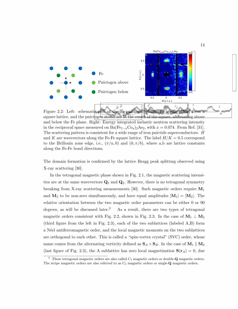
Inelastic neutron scattering measurements present an excellent characterization of the

magnetic structure in these materials. Fig. 2.2 shows energy-integrated inelastic neutron

scattering in Ba(Fe1−xCox)2As2 in the Brillouin zone of the one-Fe unit cell.1 Dif-

ferent families of iron pncitide/chalcogenides exhibit similar structures. The scattering

intensities are peaked at wavevectors Q1 = (π, 0) and Q2 = (0, π), commensurate with

the underlying lattice. We can therefore introduce two magnetic order parameters M1

and M2 associated with the two wavevectors, and write the real space magnetization

as:

S(r) = M1 cos(Q1 · r) + M2 cos(Q2 · r) (2.1)

Since Qi are commensurate with the underlying lattice, due to inversion symmetry,

Mi are real three-component vector fields.

In most of the iron pnictide materials such as Ba(Fe1−xCox)2As2, the magnetic

order is the stripe order, with either M1 or M2 being non-zero, therefore breaking

lattice rotation symmetry from tetragonal (C4) down to orthorhombic (C2). There are

two types of stripe magnetic orders, as shown in Fig. 2.3, where one has parallel spins

along the x-direction, and the other along the y-direction. The magnetic scattering

intensities at both M1 and M2, as shown in Fig. 2.2, are due to formation of domains.

1 The actual unit cell contains two Fe atoms, due to the puckering of the pnictogen/chalcogen atoms.Both one-Fe and two-Fe unit cells have been used in the literature.

14

Fe

Pnictogen above

Pnictogen below

2

s10

s11

v01

v02

min

max

0.5

0

-0.5

-0.5 0 0.5 -0.5 0 0.5

-0.5 0 0.5 -0.5 0 0.5

4

2

0

2

1

0

K(r

.l.u

.)

H (r.l.u.) H (r.l.u.)

K in 12 K, 1

2 K (r.l.u.) K in 12 K, 1

2 K (r.l.u.)Inte

nsity

(arb

.units)

Inte

nsity

(arb

.units)

Ba(Fe0.925Mn0.075)2As2 Ba(Fe0.926Co0.074)2As2

ı

ȷ

Qstripe

Q Neel

T=6 K E =10 5meV

a

b

c

d

FIG. 1. (a) Spin excitations in Ba(Fe0.925Mn0.075)2As2 as mea-sured on SEQUOIA with incident energy Ei = 74.8meV and thecrystallographic c-axis parallel to the incident beam. Data are dis-played in the (H + K, H − K) plane and averaged over an energytransfer of E = 5–15 meV. Because of the fixed crystal orienta-tion with incident beam, the L component of the wavevector variesslightly with the in-plane wavevector and energy transfer. The in-dicated vectors are Qstripe = ( 1

2, 12, L≈ 1) [H= 1

2,K=0], QNeel =

(1, 0, L≈1) [H= 12,K= 1

2] in the coordinate system of the I4/mmm

tetragonal lattice. (b) A cut of the Mn-doped data (black sym-bols) and estimated phonon background (shaded symbols) alongthe [K, −K]-direction through

!12, 12

", as indicated by the dashed

line in (a). (c) Spin excitations in Ba(Fe0.926Co0.074)2As2 aver-aged over an energy transfer range of 5–15 meV as measured onthe ARCS spectrometer with Ei = 49.8meV and the c-axis paral-lel to the incident beam. (d) A cut of the Co-doped data (blacksymbols) and background (shaded symbols) along the [K, −K]-direction through

!12, 12

". In (a) and (c), an estimate of the in-

strumental background has been subtracted.

QUOIA, HB1A, and HB3 neutron spectrometers at theOak Ridge National Laboratory. The neutron scatteringdata are described in the tetragonal I4/mmm coordi-nate system with Q = 2π

a (H + K) ı + 2πa (H − K) ȷ +

2πc Lk = (H + K, H − K, L) where a = 3.97 A and

c = 12.80 A at T = 15K. In tetragonal I4/mmm no-tation, Qstripe =

!12 , 1

2 , 1"

[H= 12 , K=0] and QNeel =

(1, 0, 1) [H= 12 , K= 1

2 ]. H and K are defined to con-veniently describe diagonal cuts in the I4/mmm basalplane as varying H (K) corresponds to a longitudinal[H, H ] scan (transverse [K, −K] scan) through Qstripe.It can be shown that H and K are the reciprocal lat-tice units of the Fe square lattice discussed above since

Q = 2πaFe

#H 1√

2(ı + ȷ) + K 1√

2(ı − ȷ)

$= (H, K), where

aFe = a√2

is the nearest-neighbor Fe-Fe distance. Thus,

Qstripe = (12 , 0) and QNeel = (1

2 , 12 ) in Fe square lattice

notation.

Figure 1(a) shows background subtracted data in thestripe AFM ordered phase at T = 6K and an energytransfer E = 10 meV. Sharply defined peaks are ob-served near Qstripe = (1

2 , 12 , 1) and symmetry related

wavevectors corresponding to spin waves in the stripeAFM state .Broad inelastic scattering is also observedat QNeel = (1, 0, 1) and symmetry related wavevec-tors .A transverse cut along the [K, −K]-direction inFig. 1(b) highlights the strong inelastic scattering at bothQstripe and QNeel. Previously published data on Co-doped Ba(Fe0.926Co0.074)2As2 find no such excitationsat QNeel.[14] At this comparable doping level, the Co-doped sample is paramagnetic and superconducting, andFigs. 1(c) and 1(d) show only a broad peak at Qstripe

originating from stripe spin fluctuations common to alliron-based superconductors.[14]

It is at first unclear whether the inelastic scatteringintensity observed in the Mn-doped sample at QNeel ismagnetic or nuclear in origin, since (1, 0, 1) is a nuclearBragg peak in the I4/mmm space group. The absenceof any inelastic peak in Co-doped materials near QNeel

suggests that it does not arise from phonons in the vicin-ity of the (1, 0, 1) nuclear peak. Perhaps the strongestevidence for the magnetic origin of this feature comesfrom measurements along the (1, 0, L) direction using theHB1A triple-axis spectrometer, shown in Fig. 2(a). AtT = 10K and E = 3 meV, the intensity manifests a sinu-soidal modulation peaked at odd values of L, as expectedfor antiferromagnetic spin correlations between the lay-ers. The decay of the signal at large L follows the Fe2+

magnetic form factor, thereby confirming their magneticnature.

Fig. 2(b) shows that the magnetic spectrum at Qstripe

consists of steep spin waves associated with the long-range stripe AFM order whereas, at QNeel, figs. 2(b) and(c) indicate that the spectrum has a quasielastic or re-laxational form. Therefore, Mn-doping introduces short-ranged checkerboard-like spin correlations with wavevec-tor QNeel that are purely dynamic and coexist with thelong-range stripe AFM order.

To clarify the relationship between magnetism at QNeel

and Qstripe, we studied the temperature dependence ofthe spin fluctuations, as illustrated in Fig. 3(a)-(e). Mag-netic fluctuations at QNeel are weakly temperature de-pendent and persist up to at least 300K. As expected,the excitations at Qstripe become broader above TN =80K and paramagnetic stripe spin fluctuations becomenearly washed out at 300K. This broadening occursmore strongly along the [K, −K]-direction transverse toQstripe, signaling a significant temperature dependenceof the in-plane anisotropy of the stripe spin fluctuations.

The temperature dependence of the imaginary part ofthe dynamic magnetic susceptibility χ′′(QNeel, E) andχ′′(Qstripe, E) is shown in Figs. 4(a) and 4(b), respec-tively. The susceptibility is obtained from neutron scat-tering data according to the formula

S(Q, E) ∝ f2(Q)χ′′(Q, E)(1 − e−E/kT )−1 (1)

where S(Q, E) = I(Q, E) − B(Q, E) is the magnetic in-tensity, I(Q, E) is the measured intensity, B(Q, E) is

2

s10

s11

v01

v02

min

max

0.5

0

-0.5

-0.5 0 0.5 -0.5 0 0.5

-0.5 0 0.5 -0.5 0 0.5

4

2

0

2

1

0

K(r

.l.u

.)

H (r.l.u.) H (r.l.u.)

K in 12 K, 1

2 K (r.l.u.) K in 12 K, 1

2 K (r.l.u.)Inte

nsity

(arb

.units)

Inte

nsity

(arb

.units)


ı

ȷ

Qstripe

Q Neel

T=6 K E =10 5meV

a

b

c

d


2, 12, L≈ 1) [H= 1

2,K=0], QNeel =

(1, 0, L≈1) [H= 12,K= 1



!12, 12



!12, 12




a (H + K) ı + 2πa (H − K) ȷ +



!12 , 1

2 , 1"


(1, 0, 1) [H= 12 , K= 1


Q = 2πaFe

#H 1√

2(ı + ȷ) + K 1√

2(ı − ȷ)

$= (H, K), where

aFe = a√2




notation.













S(Q, E) ∝ f2(Q)χ′′(Q, E)(1 − e−E/kT )−1 (1)


2

s10

s11

v01

v02

min

max

0.5

0

-0.5

-0.5 0 0.5 -0.5 0 0.5

-0.5 0 0.5 -0.5 0 0.5

4

2

0

2

1

0

K(r

.l.u

.)

H (r.l.u.) H (r.l.u.)

K in 12 K, 1

2 K (r.l.u.) K in 12 K, 1

2 K (r.l.u.)Inte

nsity

(arb

.units)

Inte

nsity

(arb

.units)


ı

ȷ

Qstripe

Q Neel

T=6 K E =10 5meV

a

b

c

d


2, 12, L≈ 1) [H= 1

2,K=0], QNeel =

(1, 0, L≈1) [H= 12,K= 1



!12, 12



!12, 12




a (H + K) ı + 2πa (H − K) ȷ +



!12 , 1

2 , 1"


(1, 0, 1) [H= 12 , K= 1


Q = 2πaFe

#H 1√

2(ı + ȷ) + K 1√

2(ı − ȷ)

$= (H, K), where

aFe = a√2




notation.













S(Q, E) ∝ f2(Q)χ′′(Q, E)(1 − e−E/kT )−1 (1)


Figure 2.2: Left: schematic plot of the Fe-pnictogen plane. Fe atoms (blue) form asquare lattice, and the pnictogen atoms are at the center of the square, alternating aboveand below the Fe plane. Right: Energy integrated inelastic neutron scattering intensityin the reciprocal space measured on Ba(Fe1−xCox)2As2, with x = 0.074. From Ref. [31].The scattering pattern is consistent for a wide range of iron pnictide superconductors. Hand K are wavevectors along the Fe-Fe square lattice. The label H/K = 0.5 correspondto the Brillouin zone edge, i.e., (π/a, 0) and (0, π/b), where a,b are lattice constantsalong the Fe-Fe bond directions.

The domain formation is confirmed by the lattice Bragg peak splitting observed using

X-ray scattering [30].

In the tetragonal magnetic phase shown in Fig. 2.1, the magnetic scattering intensi-

ties are at the same wavevectors Q1 and Q2. However, there is no tetragonal symmetry

breaking from X-ray scattering measurements [30]. Such magnetic orders require M1

and M2 to be non-zero simultaneously, and have equal amplitudes |M1| = |M2|. The

relative orientation between the two magnetic order parameters can be either 0 or 90

degrees, as will be discussed later.2 As a result, there are two types of tetragonal

magnetic orders consistent with Fig. 2.2, shown in Fig. 2.3. In the case of M1 ⊥ M2

(third figure from the left in Fig. 2.3), each of the two sublattices (labeled A,B) form

a Neel antiferromagnetic order, and the local magnetic moments on the two sublattices

are orthogonal to each other. This is called a “spin-vortex crystal” (SVC) order, whose

name comes from the alternating vorticity defined as SA×SB. In the case of M1 ‖M2

(last figure of Fig. 2.3), the A sublattice has zero local magnetization S(rA) = 0, due

2 These tetragonal magnetic orders are also called C4 magnetic orders or double-Q magnetic orders.The stripe magnetic orders are also referred to as C2 magnetic orders or single-Q magnetic orders.

15

A

B

A

B

Figure 2.3: Four types of magnetic orders consistent with the inelastic neutron scatteringexperiment shown in Fig. 2.2. From left to right: stripe magnetic orders with ferromag-netic alignments along y and x directions, spin-vortex crystal (SVC) and charge-spindensity wave (CSDW) orders that preserve lattice tetragonal symmetry. A and B labelthe two sublattices that exhibit Neel antiferromagnetic order.

to the cancellation between M1 and M2. The B sublattice forms a Neel antiferromag-

netic order, where the local magnetization are twice as big. As will be shown later, this

magnetic order also induces a charge density wave order with wavevector (π, π). It is

therefore termed “charge-spin density wave” (CSDW). The tetragonal magnetic orders

have been proposed and studied in Ref. [32, 33, 34, 28, 35, 36, 37, 38].

One of the main difficulties in experiments is to disentangle features coming from

domains of C2 order and true C4 magnetic orders. The present experimental results

rely on the indirect measurement of lattice Bragg peak splitting. One objective of this

chapter is to find direct ways to distinguish between C2 and C4 magnetic orders, as well

as between the two C4 magnetic phases.

Having explained the possible types of magnetic orders in iron pnictide materials,

here I briefly describe the microscopic origin responsible for them. In Sec. 2.3 I will

present a detailed analysis of how each magnetic order can become the ground state.

Generally speaking, magnetism emerges as collective quantum mechanical behavior

of electrons, driven by electronic interactions, i.e., screened Coulomb interaction. De-

pending on whether the electronic system is metallic or insulating, there are two ways

how magnetic order can emerge.

In metallic systems, electrons are delocalized, and described by Bloch wavefunctions.

The itinerant electrons form a conduction band, and occupy states with the lowest ki-

netic energies. Electrons fill the band up to the Fermi energy, which is characterized

16

by a Fermi surface in the momentum space. In the presence of electron-electron inter-

actions, magnetism can emerge as a Fermi surface instability. This is the well-known

“Stoner criterion”. Magnetic orders due to a Fermi surface instability are itinerant in

nature, and are also called spin density wave (SDW) orders. Mathematically, the Stoner

criterion can be seen by writing down the spin susceptibility χmag using the “random

phase approximation” (RPA) of the Hubbard model discussed in Eq. 1.1:

χmag(q, T ) =χ0(q, T )

1− Uχ0(q, T )(2.2)

Here U is the onsite Hubbard repulsion (screened Coulomb repulsion), T is the tem-

perature, q the wavevector, and χ0 the non-interacting spin susceptibility due to the

Fermi surface. In the simplest case of an isotropic Fermi liquid, χ0(q, T → 0) ≈Nf [1− 1

3(q/kf )2], where kf is Fermi wavevector, and Nf the electronic density of states

at the Fermi level. The spin susceptibility becomes divergent at q = 0 at a critical inter-

action strength 1 = UcNf , signaling the onset of ferromagnetic order. SDW orders with

a finite ordering wavevector Q are possible, if the Fermi surface has special “nesting”

properties, i.e., εk = −εk+Q, where εk is the energy dispersion of the itinerant electrons.

In this case, χ0(q, T ) ≈ Nf [ln(Λc/T )− (q−Q)2], where Λc is some upper energy cutoff.

The onset temperature of SDW order is determined by 1 = NfU ln(Λc/TSDW). Due to

nesting, there is a finite transition temperature for arbitrarily weak interactions.

In the other scenario, magnetism can emerge from a Mott insulating phase. A Mott

insulator is driven due to strong electronic interactions. For a half-filled band, since

there is an odd number of electrons per unit cell, the electrons should be delocalized

as there is no Pauli’s principle preventing it. However, strong electronic interactions

prevent one electron to hop from site to site, leaving a vacancy on the original site and

a double-occupancy on the other. In a Mott insulator, mobile charge degrees of freedom

are frozen, however, localized electronic spins can interact with each other from “virtual

hopping” [39], and the electronic model is mapped onto a spin-Heisenberg model:

H = J∑

〈ij〉Si · Sj (2.3)

where S ≡ 12c†~σc is the spin operator, and J > 0 is the antiferromagnetic spin-spin

interaction. Starting from the t-U Hubbard model, J ∝ t2/U [39].

17

The different origins for magnetism are due to a difference in the electronic inter-

action strength. For a weakly interacting system, electrons delocalize to form a metal,

whereas for a strongly interacting system, electrons localize to become a Mott insula-

tor. In the itinerant picture, the SDW order is driven by a gain in the Coulomb energy,

while in the localized picture, magnetism is driven by a gain in the kinetic energy, i.e.,

tendency toward delocalization.

Which of these two pictures is more suitable for describing magnetism in iron pnictide

superconductors? Combined experimental and theoretical results show that electronic

interactions in these materials are in the intermediate range. On the one hand, the

disordered state from which magnetism emerges is metallic. Quantum oscillations on

the parent compounds of iron pnictide materials show well-defined Fermi surfaces at

low temperatures[40]. On the other hand, optical conductivity measurements Ref. [41]

suggest that the electronic kinetic energy in LaFeAsOP is suppressed by a factor of

2. Ref. [42] also show significant electronic mass renormalization from density function

theory calculation.

In the rest of the chapter, I will address both the nature and the origin of magnetism

by carefully comparing predictions of localized versus itinerant model with experimental

results, and in particular, which picture is more suitable for the study of tetragonal

magnetic orders. Additionally, I will propose additional experimental signatures which

can be used to uniquely identify the magnetic order in iron pnictide superconductors.

This chapter closely follows our published works in Ref. [35, 36, 37].

2.2 Ginzburg-Landau analysis

The discussion in this section is based on my paper Ref. [35, 36].

To see how the single-Q and double-Q magnetic orders emerge, we write down the

Ginzburg-Landau free energy for the order parameters (M1,M2) defined previously,

constrained by O(3) spin rotation and inversion symmetry and C4 lattice rotation sym-

metry:

F =∑

i=1,2

(r

2M2

i +β

4M4

i

)+α

2M2

1M22 + w(M1 ·M2)2 (2.4)

18

Here we introduced the notation: M4i ≡ (M2

i )2, and M2

i ≡Mi ·Mi. Mi=1,2 is a three-

component vector order parameter. r ∝ T − TN measures the distance to a mean-field

magnetic phase transition. The coupling between M1 and M2 starts at quartic order,

as the bilinear term (M1 ·M2) has a finite momentum. The free energy can be rewritten

as:

F =r

2(M2

1 + M22) +

u

4(M2

1 + M22)2 − g

4(M2

1 −M22)2 + w(M1 ·M2)2 (2.5)

where u ≡ (α + β)/2, and g ≡ (α − β)/2. This form is used in Ref. [35, 36] to analyze

the possible magnetic states.

The first two terms depend only on the combination M21 + M2

2, effectively enlarging

the symmetry of the system to O(6), and resulting in a huge degeneracy of the magnetic

ground state [33, 43]. The last two terms are responsible for lifting this degeneracy,

selecting both the relative amplitudes (either M21/M

22 = 0 or M2

1/M22 = 1) and the

relative orientations of the two order parameters (either M1 ‖ M2 or M1 ⊥ M2).

Fig. 2.4 displays the phase diagram and the resulting ground states as function of g and

w at the mean-field level. For g > max 0,−w, we find a stripe state, characterized

by M1 6= 0 and M2 = 0 (or vice-versa), which breaks the tetragonal symmetry of the

system. This is the state most commonly observed in the iron pnictides and has a

residual Z2 (Ising) symmetry, related to choosing either M1 6= 0 or M2 6= 0, which

can be broken even before the magnetic transition takes place [44]. This residual order,

called the spin-nematic order, will be the main topic of interest in Ch. 3.

For g < max 0,−w, minimization of the free energy leads to a tetragonal magnetic

state characterized by simultaneously non-vanishing M21 = M2

2. Two different configu-

rations are possible: for w > 0, we obtain the SVC state M1 ⊥ M2, see Fig. 2.4 and

also Refs. [32, 33]. For w < 0, the ground state is given by M1 ‖ M2, corresponding

to a CSDW state. This state induces a charge density-wave (CDW) with modulation

Q1 + Q2 = QN , where the odd (non-magnetic) sites have different local charge than

the even (magnetic) sites. This can be seen from Eq. 2.5 by including the Ginzburg-

Landau term ζ ρQN(M1 ·M2) [45], which leads to a non-zero CDW order parameter

ρQN= χCDWζ (M1 ·M2), whose amplitude depends on both the coupling constant ζ

and the bare CDW susceptibility χCDW.

While the vast majority of iron pnictides display a stripe ground state, g > max 0,−w,

19

g

w

SV C

CSDW

Stripe

Figure 2.4: Mean field phase diagram of the Ginzburg-Landau free energy, displayingthe stripe state for g > max 0,−w, as well as the spin-vortex crystal and charge-spindensity wave states for g < max 0,−w. Adapted from our work Ref. [35]. See alsoRef. [32, 33].

the observations of a tetragonal magnetic state [26, 27, 28, 29] indicate that a change

in the microscopic system parameters can change the Ginzburg-Landau coefficients and

bring the system to the regime of the double-Q magnetic states.

2.3 Microscopic origin for magnetism

As was briefly discussed in the introduction, depending on the electronic interaction

strength, the microscopic origin for magnetism is different. In the localized picture,

magnetism emerges due to spin-spin exchange interactions. In the itinerant picture,

magnetism is a Fermi surface instability. Here I will elaborate both scenarios, and

show how the three types of magnetic orders can/cannot emerge from each scenario.

In particular, as I will show later, neither of the two C4 magnetic orders (CSDW and

SVC) can be obtained from a localized J1-J2 Heisenberg model, whereas in an itinerant

picture, they appear naturally due to the low-energy electronic properties.

20

2.3.1 Multi-orbital Hubbard model for iron pnictide materials

As has been discussed in Ch. 1, due to the crystal environment and the 3d6 electronic

configuration of Fe2+, a low-energy description of the iron pnictide materials should

include all five d orbitals. A microscopic model is the multi-orbital Hubbard model,

discussed in Ref. [21]. The kinetic Hamiltonian is described as:

H0 =∑

ij,µν

∑

σ

tµi,νjd†µ,iσdν,jσ (2.6)

where d†µ,iσ creates an electron at site i and orbital µ = 1...5 with spin state σ. tµi,νj

are hopping amplitudes. The diagonal terms describe the band dispersions of electrons

from separate orbitals, while the off-diagonal terms describe the hybridization. Due to

the multi-orbital nature, there are at least four onsite interaction terms:

Hint = U∑

i,µ

nµ,i↑nµ,i↓ + J∑

i,µ<ν

∑

σ,σ′d†µ,iσd

†ν,iσ′dµ,iσ′dν,iσ

+ U ′∑

i,µ<ν

nµ,inν,i + J ′∑

i,µ 6=νd†µ,i↑d

†µ,i↓dν,i↓dν,i↑

(2.7)

Here U is the usual Hubbard repulsion between electrons on the same orbitals, U ′ is the

onsite repulsion between electrons on different orbitals, J is the Hund’s exchange that

tends to align spins at different orbitals, and J ′ is another exchange term, often called

the pair-hopping term.

Eq. 2.6 and 2.7 defines the five-orbital Hubbard model. This is a very complicated

model to solve beyond self-consistent mean field theory, in particular, if the kinetic term

and the interaction term are comparable. In the following sections, I describe the two

limits where we can have tractable analytical solutions in regards to magnetism, namely,

the strong coupling limit and the weak coupling limit.

2.3.2 Localized J1-J2 Heisenberg model

If the electronic interactions are strong, we can project out the charge degrees of free-

dom, to arrive at some form of spin-Heisenberg model. However, due to the multi-orbital

nature, the projection is quite complicated[46, 47]. Instead, a Heisenberg model with

both nearest-neighbor (J1) and next-nearest-neighbor (J2) antiferromagnetic interac-

tions has been proposed as a phenomenological model. The Heisenberg Hamiltonian is

21

defined as:

H = J1

∑

〈ij〉Si · Sj + J2

∑

〈〈ij〉〉Si · Sj (2.8)

where 〈· · · 〉 and 〈〈· · · 〉〉 label nearest neighbor and next-nearest-neighbor respectively.

Depending on the ratio of J1/J2, different magnetic orders are stabilized.

Classically, when J1/J2 > 2, the ground state is the Neel antiferromagnetic order,

with nearest-neighbor spins antiparallel to each other. When J1/J2 < 2, the next-

nearest-neighbor interaction is dominant, and the lattice splits into two sublattices of

Neel order along the diagonal directions, see Fig. 2.3. At a classical level, the relative

angle θ between spin orientations on the two sublattices is not fixed by J1 6= 0. This

is because any given spin on one sublattice is surrounded by four neighboring spins

on a different sublattice, and due to the Neel configuration, the average interaction is

zero. Quantum and thermal fluctuations can break this classical degeneracy, and favor

θ = 0 or π, corresponding to either of the two stripe configurations described in Fig. 2.3.

This is the so-called ”order-from-disorder” effect studied in Ref. [48]. Microscopically,

the effect of quantum and thermal fluctuations can be incorporated into a biquadratic

interaction between nearest-neighbors:

H = J1

∑

〈ij〉Si · Sj + J2

∑

〈〈ij〉〉Si · Sj −K

∑

〈ij〉(Si · Sj)2 (2.9)

where K > 0 favors the stripe state at classical level. For K < 0, the ground state

has θ = π/2, corresponding to the SVC order shown in Fig. 2.3. However, I emphasize

that K < 0 cannot be achieved by the order from disorder phenomenon of the J1-J2

Heisenberg model.

It is obvious to see that the CSDW phase cannot be achieved in the J1-J2-K Heisen-

berg model, which always has a finite (fixed) magnetization at every Fe site. The absence

of either of the C4 magnetic orders (SVC and CSDW) is a main result from the study

of this simple localized spin-Heisenberg Hamiltonian.

2.3.3 Itinerant picture and the three band model

This section is written based on my work Ref. [35, 36].

In the weak coupling scenario, the electronic interactions in Eq. 2.7 are small com-

pared to the bandwidth, and electrons are delocalized to form a conduction band. In

22

4

! X M !

"2

"1

0

1

2

3

0 Π

kx!a

0

Π

k y!a

Α1 Α2 Β1

Β2

dxzdyzdxz"dyzdx2"y2

dxyd3&z2"r2

"a#

"b#

FIG. 5: (Color online) (a) The backfolded band structure for the 5band model with Γ, X, and M denoting the symmetry points in thereal Brillouin zone corresponding to the 2 Fe unit cell. The mainorbital contributions are shown by the following colors: dxz (red),dyz (green), dxy (yellow), dx2−y2 (blue), d3z2−r2 (magenta), anda strongly hybridized dxz-dyz band (brown). The gray lines showthe correct DFT band structure calculated by Cao et al. (b) The FSsheets of the 5 band model for the undoped compound (x = 0).

function

(χ1)st (q, iω) =

1

3

! β

0

dτ eiωτ"Tτ Ss(q, τ)St(−q, 0)

#(8)

with τ the imaginary time andω aMatsubara frequency. In thesame way we can define the Fourier component of the chargedensity for the orbital s as

ns(q) =$

k,αβ

d†sα(k + q)dsβ(k)δαβ (9)

and we can calculate the charge susceptibility from

(χ0)st (q, iω) =

! β

0

dτ eiωτ ⟨Tτns(q, τ)nt(−q, 0)⟩ (10)

In a more general formulation the susceptibilities are func-tions of four orbital indices. For the non-interacting case

FIG. 6: (Color online) The orbital weights as a function of the wind-ing angle φ on the different Fermi surface sheets. The different colorsrefer to dxz (red), dyz (green), dxy (yellow), dx2−y2 (blue), d3z2−r2

(magenta).

(χ0)pqst and (χ1)

pqst are equivalent and can be written

χpqst (q, iω) =

! β

0

dτ eiωτ$

kk′

$

αβ

⟨Tτd†pα(k, τ) (11)

dqα(k + q, τ)d†sβ(k′, 0)dtβ(k′ − q, 0)⟩

Now we can derive an explicit expression for the non-interacting susceptibilities from

χpqst (q, iω) = − 1

Nβ

$

k,iωn

Gsp(k, iωn)Gqt(k + q, iωn + iω)

(12)where N is the number of Fe lattice sites, β = 1/T , and thespectral representation of the Green’s function is given as

Gsp(k, iωn) =$

µ

asµ(k)ap∗

µ (k)

iωn − Eµ(k)(13)

Here the matrix elements asµ(k) = ⟨s|µk⟩ connect the orbital

and the band space and are the components of the eigenvectorsresulting from the diagonalization of the initial Hamiltonian.Performing the Matsubara frequency summation and settingiωn → ω + i0+ we find the retarded susceptibility

χpqst (q,ω) = − 1

N

$

k,µν

asµ(k)ap∗

µ (k)aqν(k + q)at∗

ν (k + q)

ω + Eν(k + q) − Eµ(k) + i0+

× [f(Eν(k + q)) − f(Eµ(k))] (14)

X

Y

M1

M2

Figure 2.5: Left: Fermi surface obtained from tight-binding fit to LDA calculations ofiron pnictide band structure. Taken from Ref. [49]. Right: Simplified three band modeldescribing itinerant magnetism.

the itinerant picture, magnetism comes from Fermi surface instability. Below I will

first discuss how the Ginzburg-Landau free energy can be obtained from the itinerant

picture, following the Hertz-Millis approach[22, 23]. Then I will discuss the microscopic

origins of how various magnetic orders can be stabilized.

The outer shell of the Fe2+ ion has 3d6 configuration. LDA calculation shows that all

five Fe 3d orbitals are located near the Fermi level[50]. Fig. 2.5 shows a tight binding fit

of the Fermi surface to the LDA calculation [49]. There are two hole-like Fermi pockets

centered at the Γ point (zone center), and two electron-like Fermi pockets centered at

X and Y (zone boundary).

The outer hole pocket and the electron pockets are of similar sizes, and are quasi-

nested (εh,k ≈ −εei,k+Qi) with wavevector Qi. As a result, the charge/spin fluctuations

with Qi are strongly enhanced by the nesting of the Fermi surface. To study magnetism

in the itinerant picture, it is convenient to neglect the orbital character of the Fermi

surface, and work in the band basis. The small internal hole pocket can also be neglected

because it is less nested with other Fermi surfaces. As a result, we can construct a low-

energy effective three-band model as depicted in Fig. 2.5. The band dispersions of the

23

hole and electron pockets can be approximated as[33]:

εh,k = ε0 −k2

2m− µ

εe1,k+Q1 = −ε0 +k2x

2mx+

k2y

2my− µ

εe2,k+Q2 = −ε0 +k2x

2my+

k2y

2mx− µ

(2.10)

where µ is the chemical potential, ε0 an energy shift, and mx 6= my defines the ellipticity

of the electron pockets. Close to particle-hole symmetry (perfect nesting), we can rewrite

the band dispersions in a more convenient form:

εh,k = −εkεe1,k+Q1 = εk − (δµ + δm cos 2θ)

εe2,k+Q2 = εk − (δµ − δm cos 2θ)

(2.11)

where θ is the angle around the Fermi surface. The parameter δµ is related to the

occupation number (doping) and δm to the ellipticity of the electron pockets:

δµ = 2µ+ εF

[1− m

2

(mx +my

mxmy

)]

δm =εFm

2

(mx −my

mxmy

) (2.12)

The non-interacting Hamiltonian is given by H0 =∑

k,a εk,ac†a,kαca,kα, with band index

a and spin index α.

Following Ref. [51, 52], there are eight types of purely electronic interactions con-

necting the three Fermi pockets which preserves the spin rotation symmetry. They are

the density-density (U1, U4, U5, U6), spin-exchange (U2, U7) and pair-hopping (U3, U8)

interactions respectively. The interaction Hamiltonian is:

Hint = U1

∑c†hαc

†eiβceiβchα + U2

∑c†hαc

†eiβchβceiα

+U3

2

∑(c†hαc

†hβceiβceiα + h.c.)

+U4

2

∑c†eiαc

†eiβceiβceiα +

U5

2

∑c†hαc

†hβchβchα

+ U6

∑c†e1αc

†e2βce2βce1α + U7

∑c†e1αc

†e2βce1βce2α

+U8

2

∑(c†e1αc

†e1βce2βce2α + h.c.)

(2.13)

24

For simplicity of notation, the momentum indices are all suppressed with the im-

plicit constraint of momentum conservation. Note that such eight types of interactions

can be derived from a microscopic Hamiltonian, e.g., the multi-orbital Hubbard model

described in Eq. 2.6.

To study the instability towards magnetic order, we project all the interactions in

the spin-density wave (SDW) channel – which is the leading one according to RG and

fRG calculations [52, 53]. The only interactions that contribute directly to the SDW

instability are U1 and U3. The partition function, restricted to this channel only, can

then be written in the functional field form:

Z =

∫Dc†Dc exp(−S) (2.14)

with the action:

S =

∫ β

0dτ

∑

ikσ

c†ikσ∂τ cikσ +H0 +HSDW (2.15)

and the SDW-decoupled interaction:

HSDW = −I∑

ikk′q

(c†hkασαβceik+qβ

)·(c†eik′γσγδchk′−qδ

)(2.16)

where I = U1 + U3. We now introduce the Hubbard-Stratonovich field Mi, whose

mean value is proportional to the staggered magnetization with ordering vector Qi, i.e.

〈Mi〉 = I∑

k

⟨c†hkασαβceik+qβ

⟩, via exp (−HSDW) ∝

∫DMi exp (−SSDW [Mi]) with:

SSDW [Mi] =∑

iq

Miq ·Mi−qI

−∑

iqk

(Miq · c†eikγσγδchk−qδ + h.c.

)(2.17)

Following Ref. [44], we then integrate out the electronic degrees of freedom, obtaining

an effective action for the magnetic degrees of freedom:

Z =

∫Dc†DcDMi exp

(−S

[c†,Mi

])

=

∫DMi exp (−Seff [Mi]) (2.18)

For a finite-temperature magnetic transition, Seff [Mi] = F [Mi] /T , where F [Mi] is

the free energy. Near the magnetic transition, we can expand the action in powers of

the magnetic order parameters, deriving the Ginzburg-Landau expansion:

Seff [Mi] =r

2(M2

1 + M22) +

u

4(M2

1 + M22)2 − g

4(M2

1 −M22)2 + w(M1 ·M2)2 (2.19)

25

This is identical to the phenomenological Ginzburg-Landau free energy presented

in Eq. 2.5, but now the coefficients are given microscopically. In the vicinity of the

magnetic transition, r ≈ Nf (T − TN ), where Nf is the density of states at the Fermi

surface. The coefficients u, g, and w are given by [44]:

u = A+B; g = B −A; w = 0 (2.20)

with:

A =

∫

kG2h,kG

2e1,k+Q1

=

∫

k

(1

iωn + εk

)2( 1

iωn − εk + δµ + δm cos 2θ

)2

B =

∫

kG2h,kGe1,k+Q1Ge2,k+Q2

=

∫

k

(1

iωn + εk

)2 1

iωn − εk + δµ + δm cos 2θ

1

iωn − εk + δµ − δm cos 2θ

(2.21)

Here, Ga,k is the non-interacting fermionic Green’s function for pocket a, G−1a,k =

iωn − εa,k, and∫k → T

∑n

∫dk

(2π)d, with Matsubara frequency ωn = (2n+ 1)πT . After

integrating out the momentum, we obtain:

A = NfTπ∞∑

n=0

Im

∫

θ

1(iωn +

δµ2 + δm

2 cos 2θ)3

B = NfTπ

∞∑

n=0

Im

∫

θ

iωn +δµ2((

iωn +δµ2

)2−(δm2 cos 2θ

)2)2 (2.22)

with∫θ =

∫ 2π0

dθ2π .

In the limit of perfect nesting (i.e. δµ = δm = 0) one obtains g = w = 0, implying

that the system has an enlarged O(6) symmetry and a huge ground-state degeneracy.

Expanding near perfect nesting yields w = 0 and:

u =

∫

kG2h,k (Ge1,k +Ge1,k)

2 ≈ 7ζ(3)NF

2π2T 2(2.23)

g =

∫

kG2h,k (Ge2,k −Ge2,k)2 ≈ 31ζ(5)NF

32π4T 2

(δmT

)2

> 0 (2.24)

26

This places the system in the regime of a stripe magnetic state (see Fig. 2.4). Similar

free energy calculations considering other types of band dispersions also find that the

stripe state is favored for a wide range of parameters, consistent with the observations

that most iron pnictides display this magnetic ordered state [32, 34, 54, 55].

How can C4 magnetic phases be favored in this itinerant model? Below I discuss two

effects that can drive a phase transition from the C2 magnetic phase to the C4 magnetic

phases, namely, moving away from perfect nesting, based on my paper Ref. [36], and

the effect of Neel antiferromagnetic fluctuations based on my paper Ref. [35].

2.3.4 Away from perfect nesting

This section is written based on my paper Ref. [36].

In the previous section, we showed that within the microscopic three-band model,

small deviations from perfect-nesting lead to a stripe magnetic order. In this section,

we show that strong deviations from particle-hole symmetry (perfect nesting) favor a

tetragonal magnetic state over the stripe state. Interestingly, the SVC state is selected

by a residual electronic interaction that does not participate explicitly in the formation

of the magnetic state (Ref. [33]). These theoretical results are complementary to those

reported in Ref. [28, 29, 26], which found that deep inside the stripe ordered state a

second instability towards a tetragonal magnetic state emerges.

The previous analysis of the Ginzburg-Landau coefficients (2.22) in Ref. [44] focused

on the regime near perfect nesting, where δµ, δm T . In this case, g ∝ δ2m > 0 and

the ground state is the stripe magnetic one. Here, we extend the analysis beyond small

deviations from perfect nesting by numerically computing Eqs. 2.22 for arbitrary δµ/T ,

δm/T .3

The effect of doping is mimicked by changing the parameter δµ (proportional to

the carrier concentration) for a fixed value of the ellipticity δm. Note that Eq. 2.22

implies that the behavior of u and g depend only on |δµ|. Fig 2.6 shows the results for

δm/T = 0.8π and δm/T = 2π. For small values of |δµ|, both u and g are positive, and the

stripe magnetic state is favored. However, as |δµ| becomes larger, regardless of the value

3 Here T ≈ TN . The constraint δm ≥ δµ is imposed to ensure that hot spots are present, as seenexperimentally. Hot spots are locations on the electron/hole Fermi surfaces that are connected by theSDW wavevector Qi=1,2.

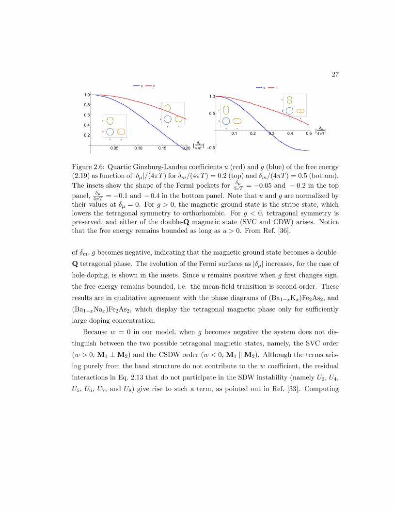
27

g u

0.05 0.10 0.15 0.20|

δμ

4πT|

0.2

0.4

0.6

0.8

1.0

0 π

0

π

0 π

0

π

g u

0.1 0.2 0.3 0.4 0.5|

δμ

4πT|

-0.5

0.5

1.0

0 π

0

π

0 π

0

π

Figure 2.6: Quartic Ginzburg-Landau coefficients u (red) and g (blue) of the free energy(2.19) as function of |δµ|/(4πT ) for δm/(4πT ) = 0.2 (top) and δm/(4πT ) = 0.5 (bottom).

The insets show the shape of the Fermi pockets forδµ

4πT = −0.05 and − 0.2 in the top

panel,δµ

4πT = −0.1 and −0.4 in the bottom panel. Note that u and g are normalized bytheir values at δµ = 0. For g > 0, the magnetic ground state is the stripe state, whichlowers the tetragonal symmetry to orthorhombic. For g < 0, tetragonal symmetry ispreserved, and either of the double-Q magnetic state (SVC and CDW) arises. Noticethat the free energy remains bounded as long as u > 0. From Ref. [36].

of δm, g becomes negative, indicating that the magnetic ground state becomes a double-

Q tetragonal phase. The evolution of the Fermi surfaces as |δµ| increases, for the case of

hole-doping, is shown in the insets. Since u remains positive when g first changes sign,

the free energy remains bounded, i.e. the mean-field transition is second-order. These

results are in qualitative agreement with the phase diagrams of (Ba1−xKx)Fe2As2, and

(Ba1−xNax)Fe2As2, which display the tetragonal magnetic phase only for sufficiently

large doping concentration.

Because w = 0 in our model, when g becomes negative the system does not dis-

tinguish between the two possible tetragonal magnetic states, namely, the SVC order

(w > 0, M1 ⊥M2) and the CSDW order (w < 0, M1 ‖M2). Although the terms aris-

ing purely from the band structure do not contribute to the w coefficient, the residual

interactions in Eq. 2.13 that do not participate in the SDW instability (namely U2, U4,

U5, U6, U7, and U8) give rise to such a term, as pointed out in Ref. [33]. Computing

28

h, µ

ei, ν

Miσµν

e2, αe1, α

h, µ

e1, β e2, β

h, ν

M1 M2

M1 M2

e2, αe1, α

h, µ

e1, β e2, β

h, ν

M1 M2

M1 M2

Figure 2.7: Top panel: The vertex that couples the magnetic order parameter to thelow-energy fermionic states, which has a Mi · σ structure. Solid lines refer to thenon-interacting electronic Green’s functions. Bottom panel: the Feynman diagramscontaining the leading-order corrections to the free energy arising from the residual U7

interaction, denoted by the dashed line. From Ref. [36].

the contributions of the residual interactions to the action, we obtain:

S [Mi] =1

4(−u2 + u4 + u5 + u6 − u7 + u8)

(M2

1 + M22

)2

− 1

4(−g4 + g6 − g7 + g8)

(M2

1 −M22

)2

+ w7 (M1 ·M2)2 (2.25)

The Ginzburg-Landau coefficients can be obtained in a straightforward way using

diagrammatics. In Fig. 2.7 we show the two diagrams arising from the U7 interaction,

which contribute to u7, g7, and w7. Additional computational details are discussed in

29

the appendix to Ref. [36]. The coefficients of the quartic symmetric term are given by:

u2 = 8U2

(∫

kGh,kG

2e1,k+Q1

)(∫

kG2h,kGe1,k+Q1

)

u4 = 2U4

(∫

kGh,kG

2e1,k+Q1

)2

u5 = 4U5

(∫

kG2h,kGe1,k+Q1

)2

u6 = 2U6

[2

(∫

kGh,kG

2e1,k+Q1

)2

−(∫

kGh,kGe1,k+Q1Ge2,k+Q2

)2]

u7 = 2U7

(∫

kGh,kG

2e1,k+Q1

)2

u8 = 2U8

(∫


)2

(2.26)

whereas the coefficients of the quartic anti-symmetric term read:

g4 = 2U4

(∫

kGh,kG

2e1,k+Q1

)2

g6 = 2U6

[2

(∫

kGh,kG

2e1,k+Q1

)2

−(∫


)2]

g7 = 2U7

(∫

kGh,kG

2e1,k+Q1

)2

g8 = 2U8

(∫


)2

(2.27)

and the coefficient of the quartic scalar-product term yields:

w7 = 4U7

(∫


)2

(2.28)

At perfect nesting, an overall factor proportional to the Green’s functions product(∫kG

2h,kGe1,k+Q1

)2appears in all terms. In this limit, our results become identical

to those found in Ref. [33], which computed the corrections to the magnetic ground

state energy in the ordered state using a sequence of Bogoliubov transformations. In

the paramagnetic state, however, which is our case of interest, this Green’s functions

product vanishes – as also pointed out in Ref. [33]. The corrections due to the residual

interactions naturally become non-zero – and in fact positive – once one considers small

30

deviations from perfect nesting. For w7, we find:

w7 ≈ 4U7

(7ζ(3)Nfδµ

8π2T 2

)2

(2.29)

Because the band dispersions do not contribute to the term (M1 ·M2)2, the fact that

w7 > 0 is very important, as it implies that the residual interaction U7 selects the SVC

state over the CSDW state (assuming that U7 > 0, as one would expect). Therefore,

when geff = g + g changes sign, the system tends to form the SVC state shown in

Fig. 2.3 and Fig. 2.4. Dimensional analysis of the relevant Feynman diagrams reveals

that g/g ∝ UiNf , where Ui is the appropriate combination of residual interactions.

Therefore, in our weak-coupling approach, because UiNf 1, it follows that g g

– unless g itself is close to zero. As a result, although the contribution from g may

change slightly the value of δµ for which geff = g + g vanishes, it cannot preclude

the sign-changing found in Fig. 2.6 from taking place. The case of weff = w + w is

fundamentally different, since w = 0, making w the leading non-vanishing term.

To conclude, although small deviations from perfect nesting (δµ/T 1 and δm/T 1) favor a stripe magnetic order, the tetragonal magnetic orders (SVC and CSDW) can

be favored for large doping levels. The residue electronic interaction U7, which is a spin-

exchange interaction between the two electron pockets centered at X and Y , favors the

SVC order over the CSDW order.

2.3.5 Neel antiferromagnetic fluctuations

This section is written based on our paper Ref. [35].

One of the first observations of C4 magnetism was in Ba(Fe1−xMnx)2As2 [30, 31].

Fig. 2.8 shows the phase diagram as a function of Mn concentration, taken from Ref. [30].

At about 10% Mn doping, the material goes from a stripe magnetic order with mea-

surable orthorhombic distortion to a magnetic order where the tetragonal symmetry is

restored. Additionally, unlike the Ba(Fe1−xCox)2As2 compounds, there is no sign of su-

perconductivity in the Mn-doped compound. A key observation from inelastic neutron

scattering experiments is that upon Mn doping, in addition to the intensities at Q1 and

Q2, there is also significant Neel fluctuations at QNeel ≡ (π, π). This is presented in

Fig. 2.8. The Neel fluctuations are most likely due to Mn dopants acting like local mag-

netic moments, evidenced by the fact that the compound BaMn2As2 is an insulating

31

temperature evolution of the AFM order is quite differentfrom what is observed for x=0.074. For x!0.118, a distinctbroadening of the magnetic peak beyond the resolution ofour measurement is observed for temperatures above T!, asdefined below and in the insets of Figs. 3!b" and 3!c".

In Fig. 4!a" we have used the neutron, x-ray and resis-tance data to construct a phase diagram in the low Mn-doping regime for Ba!Fe1−xMnx"2As2. The phase line be-tween the paramagnetic/tetragonal and AFM/orthorhombicphase for x"0.074 was easily determined from the well-defined onset of the distortion and the appearance of a reso-lution limited magnetic Bragg peak at ! 1

212 3". For x

!0.102, however, the onset of long-range magnetic order ismore difficult to identify. Therefore, we have defined a char-acteristic temperature, T!, which denotes the temperature be-low which the width of the magnetic peak is limited by ourinstrumental resolution !approximately 0.3° FWHM". Wenote that the values of T! follow the same trend seen for themaxima in dR

dT in Fig. 1. The gray band in the phase diagramrepresents the temperature range, above T!, where magneticscattering at ! 1

212 3" persists #See Figs. 3!b" and 3!c"$.

In Fig. 4!b" we plot the measured structural distortion andthe magnetic moment per Fe/Mn site, extrapolated to T=0 asdescribed in our previous work,11 as a function of dopingconcentration. Several interesting comparisons can be madebetween these results and previous x-ray and neutron scatter-ing studies of Ba!Fe1−xCox"2As2.7,9–12 First, we note that ourdata for Ba!Fe1−xMnx"2As2 for x"0.074 unambiguouslyshow that the structural and magnetic transitions remainlocked together, unlike the separation of the structural and

AFM transitions found for Co-doping. Furthermore, at x=0.102, we find a broadened magnetic peak at ! 1

212 3"

above the structural transition and, for x!0.118, we observethe magnetic Bragg peak at ! 1

212 3" in the absence of an

orthorhombic distortion, a surprising observation that will bediscussed below. Finally we note that the magnetic momentper Fe/Mn site as well as the magnitude of the structuraldistortion vary only weakly with composition for x"0.102whereas, for Co substitution, the suppression of the magneticmoment and structural distortion with doping is much moresevere.

It is also useful to compare these results to what has re-cently been found for Ba!Fe1−xCrx"2As2.24 At much higher Crconcentrations, x!0.30, Ref. 24 reports that the stripelikemagnetic structure is replaced by G-type, “checkerboard,”magnetic order as shown by polarized and unpolarized neu-tron diffraction measurements of the integrated intensity ofthe !1 0 1" Bragg peak !Fig. 3 in Ref. 24". G-type AFM orderhas been proposed for the parent BaCr2As2 compound,26 andmeasured for BaMn2As2,25 so it is not unreasonable to expectthis change in magnetic structure at high enough Cr, or Mn,doping. However, our unpolarized neutron diffraction mea-surements of the !1 0 1" peaks for the highest Mn concentra-tions, x=0.147 and 0.176, find no evidence of G-type order-ing below T=300 K. More specifically, we find nosignificant change in the !1 0 1" peak between 12 and 300 K.We cannot exclude G-type ordering that develops well aboveroom temperature given the high ordering temperature of theparent compound25 but view this as unlikely in light of thesubstantial dilution of Mn in our samples. For both Cr-andMn-doping, the moment per Fe-site remains constant !Cr", ordecreases only weakly !Mn" with increasing concentrationup to x%0.20. Indeed, as the dashed line in Fig. 4!b" shows,the decrease in the measured moment is consistent with thedecreasing Fe concentration implying that the Mn momentdoes not contribute to the magnetic AFM order characterizedby the ! 1

212 1" propagation vector. Furthermore, for Mn

doping we find an increase in the characteristic temperature!T!" associated with magnetic ordering with this propagationvector for x#0.102 whereas for Cr-doping, the orderingtemperature for this propagation vector continues to decreaseuntil the transition is completely suppressed at x=0.335,where the G-type AFM structure is observed.24 All of thispoints to interesting differences in the phase diagrams be-tween Ba!Fe1−xMnx"2As2 and Ba!Fe1−xCrx"2As2.

The observation of a magnetic structure characterized bya propagation vector of ! 1

212 1" in the absence of an ortho-

rhombic distortion !for x#0.102" is very surprising andunique to Ba!Fe1−xMnx"2As2 among the iron arsenides; mod-els for stripe-like AFM order in the iron arsenides anticipatean attendant orthorhombic distortion due to magnetoelasticeffects.12–14 Furthermore, this observation is difficult to rec-oncile with current theories that promote orbital ordering27,28

as the driving force for the stripelike magnetic phase and theorthorhombic distortion. A second key result of this study isthe qualitative change in the temperature dependence of themagnetic ordering for compositions in excess of x=0.102and the distinct broadening of the magnetic peak for T#T!.At this point it is not clear whether the scattering above T!

FIG. 4. !Color online" !a" The compositional phase diagram forBa!Fe1−xMnx"2As2 determined from neutron and x-ray diffractionmeasurements. Closed circles denote TN and open circles representT! as described in the text. Crosses denote the temperature corre-sponding to minima of dR

dT found in Fig. 1. The shaded region de-notes the extent of the magnetic scattering above T!. The verticaldashed line marks the approximate composition for the change froman orthorhombic to tetragonal structure. !b" The magnetic momentand structural distortion as a function of Mn-doping. The dashedline represents the value of the magnetic moment per Fe atom ratherthan Fe/Mn site as a function of Mn doping.

ANTIFERROMAGNETIC ORDERING IN THE ABSENCE OF… PHYSICAL REVIEW B 82, 220503!R" !2010"

RAPID COMMUNICATIONS

220503-3

temperature evolution of the AFM order is quite differentfrom what is observed for x=0.074. For x!0.118, a distinctbroadening of the magnetic peak beyond the resolution ofour measurement is observed for temperatures above T!, asdefined below and in the insets of Figs. 3!b" and 3!c".

In Fig. 4!a" we have used the neutron, x-ray and resis-tance data to construct a phase diagram in the low Mn-doping regime for Ba!Fe1−xMnx"2As2. The phase line be-tween the paramagnetic/tetragonal and AFM/orthorhombicphase for x"0.074 was easily determined from the well-defined onset of the distortion and the appearance of a reso-lution limited magnetic Bragg peak at ! 1

212 3". For x

!0.102, however, the onset of long-range magnetic order ismore difficult to identify. Therefore, we have defined a char-acteristic temperature, T!, which denotes the temperature be-low which the width of the magnetic peak is limited by ourinstrumental resolution !approximately 0.3° FWHM". Wenote that the values of T! follow the same trend seen for themaxima in dR

dT in Fig. 1. The gray band in the phase diagramrepresents the temperature range, above T!, where magneticscattering at ! 1

212 3" persists #See Figs. 3!b" and 3!c"$.

In Fig. 4!b" we plot the measured structural distortion andthe magnetic moment per Fe/Mn site, extrapolated to T=0 asdescribed in our previous work,11 as a function of dopingconcentration. Several interesting comparisons can be madebetween these results and previous x-ray and neutron scatter-ing studies of Ba!Fe1−xCox"2As2.7,9–12 First, we note that ourdata for Ba!Fe1−xMnx"2As2 for x"0.074 unambiguouslyshow that the structural and magnetic transitions remainlocked together, unlike the separation of the structural and

AFM transitions found for Co-doping. Furthermore, at x=0.102, we find a broadened magnetic peak at ! 1

212 3"

above the structural transition and, for x!0.118, we observethe magnetic Bragg peak at ! 1

212 3" in the absence of an

orthorhombic distortion, a surprising observation that will bediscussed below. Finally we note that the magnetic momentper Fe/Mn site as well as the magnitude of the structuraldistortion vary only weakly with composition for x"0.102whereas, for Co substitution, the suppression of the magneticmoment and structural distortion with doping is much moresevere.

It is also useful to compare these results to what has re-cently been found for Ba!Fe1−xCrx"2As2.24 At much higher Crconcentrations, x!0.30, Ref. 24 reports that the stripelikemagnetic structure is replaced by G-type, “checkerboard,”magnetic order as shown by polarized and unpolarized neu-tron diffraction measurements of the integrated intensity ofthe !1 0 1" Bragg peak !Fig. 3 in Ref. 24". G-type AFM orderhas been proposed for the parent BaCr2As2 compound,26 andmeasured for BaMn2As2,25 so it is not unreasonable to expectthis change in magnetic structure at high enough Cr, or Mn,doping. However, our unpolarized neutron diffraction mea-surements of the !1 0 1" peaks for the highest Mn concentra-tions, x=0.147 and 0.176, find no evidence of G-type order-ing below T=300 K. More specifically, we find nosignificant change in the !1 0 1" peak between 12 and 300 K.We cannot exclude G-type ordering that develops well aboveroom temperature given the high ordering temperature of theparent compound25 but view this as unlikely in light of thesubstantial dilution of Mn in our samples. For both Cr-andMn-doping, the moment per Fe-site remains constant !Cr", ordecreases only weakly !Mn" with increasing concentrationup to x%0.20. Indeed, as the dashed line in Fig. 4!b" shows,the decrease in the measured moment is consistent with thedecreasing Fe concentration implying that the Mn momentdoes not contribute to the magnetic AFM order characterizedby the ! 1

212 1" propagation vector. Furthermore, for Mn

doping we find an increase in the characteristic temperature!T!" associated with magnetic ordering with this propagationvector for x#0.102 whereas for Cr-doping, the orderingtemperature for this propagation vector continues to decreaseuntil the transition is completely suppressed at x=0.335,where the G-type AFM structure is observed.24 All of thispoints to interesting differences in the phase diagrams be-tween Ba!Fe1−xMnx"2As2 and Ba!Fe1−xCrx"2As2.

The observation of a magnetic structure characterized bya propagation vector of ! 1

212 1" in the absence of an ortho-

rhombic distortion !for x#0.102" is very surprising andunique to Ba!Fe1−xMnx"2As2 among the iron arsenides; mod-els for stripe-like AFM order in the iron arsenides anticipatean attendant orthorhombic distortion due to magnetoelasticeffects.12–14 Furthermore, this observation is difficult to rec-oncile with current theories that promote orbital ordering27,28

as the driving force for the stripelike magnetic phase and theorthorhombic distortion. A second key result of this study isthe qualitative change in the temperature dependence of themagnetic ordering for compositions in excess of x=0.102and the distinct broadening of the magnetic peak for T#T!.At this point it is not clear whether the scattering above T!

FIG. 4. !Color online" !a" The compositional phase diagram forBa!Fe1−xMnx"2As2 determined from neutron and x-ray diffractionmeasurements. Closed circles denote TN and open circles representT! as described in the text. Crosses denote the temperature corre-sponding to minima of dR

dT found in Fig. 1. The shaded region de-notes the extent of the magnetic scattering above T!. The verticaldashed line marks the approximate composition for the change froman orthorhombic to tetragonal structure. !b" The magnetic momentand structural distortion as a function of Mn-doping. The dashedline represents the value of the magnetic moment per Fe atom ratherthan Fe/Mn site as a function of Mn doping.

ANTIFERROMAGNETIC ORDERING IN THE ABSENCE OF… PHYSICAL REVIEW B 82, 220503!R" !2010"

RAPID COMMUNICATIONS

220503-3

2

s10

s11

v01

v02

min

max

0.5

0

-0.5

-0.5 0 0.5 -0.5 0 0.5

-0.5 0 0.5 -0.5 0 0.5

4

2

0

2

1

0

K(r

.l.u

.)

H (r.l.u.) H (r.l.u.)

K in 12 K, 1

2 K (r.l.u.) K in 12 K, 1

2 K (r.l.u.)Inte

nsity

(arb

.units)

Inte

nsity

(arb

.units)


ı

ȷ

Qstripe

Q Neel

T=6 K E =10 5meV

a

b

c

d


2, 12, L≈ 1) [H= 1

2,K=0], QNeel =

(1, 0, L≈1) [H= 12,K= 1



!12, 12



!12, 12




a (H + K) ı + 2πa (H − K) ȷ +



!12 , 1

2 , 1"


(1, 0, 1) [H= 12 , K= 1


Q = 2πaFe

#H 1√

2(ı + ȷ) + K 1√

2(ı − ȷ)

$= (H, K), where

aFe = a√2




notation.













S(Q, E) ∝ f2(Q)χ′′(Q, E)(1 − e−E/kT )−1 (1)


2

s10

s11

v01

v02

min

max

0.5

0

-0.5

-0.5 0 0.5 -0.5 0 0.5

-0.5 0 0.5 -0.5 0 0.5

4

2

0

2

1

0

K(r

.l.u

.)

H (r.l.u.) H (r.l.u.)

K in 12 K, 1

2 K (r.l.u.) K in 12 K, 1

2 K (r.l.u.)Inte

nsity

(arb

.units)

Inte

nsity

(arb

.units)


ı

ȷ

Qstripe

Q Neel

T=6 K E =10 5meV

a

b

c

d


2, 12, L≈ 1) [H= 1

2,K=0], QNeel =

(1, 0, L≈1) [H= 12,K= 1



!12, 12



!12, 12




a (H + K) ı + 2πa (H − K) ȷ +



!12 , 1

2 , 1"


(1, 0, 1) [H= 12 , K= 1


Q = 2πaFe

#H 1√

2(ı + ȷ) + K 1√

2(ı − ȷ)

$= (H, K), where

aFe = a√2




notation.













S(Q, E) ∝ f2(Q)χ′′(Q, E)(1 − e−E/kT )−1 (1)


Figure 2.8: Left panel: Phase diagram of Ba(Fe1−xMnx)2As2 as a function of Mnconcentration x, from Ref. [30]. At x < 0.12, the magnetic order is stripe type, evi-denced by the splitting of Bragg peaks observed in X-ray scattering. At x > 0.12, thepeak splitting abruptly goes to zero, while magnetism of a similar wavevector persists.Right panel: energy-integrated inelastic neutron scattering intensity, from Ref. [31]. Inaddition to the wavevectors Qi=1,2, there is a diffusive peak at QNeel, suggesting Neelantiferromagnetic fluctuations due to local moments on Mn dopants.

Neel antiferromagnet[56, 57].

To make contact with the Ba(Fe1−xMnx)2As2 compounds, we include the coupling

between the conduction electrons and the Neel fluctuations induced by the local mo-

ments. We denote by N the collective field associated with these Neel fluctuations, and

by χN (q) the corresponding momentum-dependent susceptibility. They couple to the

itinerant electrons within the three band model (Eq. 2.11) according to [58]:

HN =∑

k

N ·(c†e1,k+Q1α

σαβce2,k+Q2β

)(2.30)

where, for simplicity, the coupling constant was incorporated to N. To determine how

the magnetic instability is affected by short-range Neel fluctuations, we derive the co-

efficients of the free energy (Eq. 2.5) from the Hamiltonian H0 + HSDW + HN . The

leading corrections are quadratic in N, and:

δF =α

2N2(M2

1 + M22

)− 4λ12 [(M1 ×M2) ·N]2

+

(4λ11 + 8λ12

4

)N2(M2

1 + M22

)2

−(−4λ11 + 8λ12

4

)N2(M2

1 −M22

)2(2.31)

32

e1

he1

e2e1

h

λ11

e1

e2

h

e1e2

h

M1

NM2

λ12

(a)

0.1 0.2ΞN-1

0.01

0.02

0.03

XN2\

(b)

Figure 2.9: (a) Feynman diagrams λij associated with the coupling between the Neelcollective field N (dashed lines) and the magnetic order parameters M1 and M2 (wavylines). The solid (black) lines are the Green’s functions of the corresponding bands.(b) Behavior of the Gaussian Neel fluctuations

⟨N2⟩

as function of the inverse Neelcorrelation length ξ−1

N . The Neel critical point is at ξ−1N = 0 . From Ref. [35].

with the coefficients:

α = 4

∫

kGh,kG

2e1,kGe2,k

λij =

∫

kG2h,kGe1,kGe2,kGei,kGej ,k

The coefficients λij are represented diagrammatically in Fig. 2.9(a).

Near perfect nesting, α > 0, reflecting the competition between the Neel and stripe

states. To study the corrections to the quartic terms of the Ginzburg-Landau free energy

Eq. 2.5, we consider Gaussian isotropic Neel fluctuations (i.e., 〈NiNj〉 = 〈N2〉3 δij). We

obtain u = u + uN⟨N2⟩, g = g + gN

⟨N2⟩, and w = w + wN

⟨N2⟩. Evaluating them

near perfect nesting then gives uu ≈ 1− 0.13

〈N2〉T 2N

as well as:

g

u≈ 0.024

(δ2m

T 2N

− 4⟨N2⟩

3T 2N

);w

u≈ −0.016

⟨N2⟩

T 2N

(2.32)

where TN is the bare magnetic transition temperature. Thus, when Neel fluctuations

are strong enough compared to the energy scale of the ellipticity of the electron pock-

ets,⟨N2⟩> δ2

m/2, the leading instability of the system is towards the CSDW state

(0 < g < −w), which preserves the tetragonal symmetry of the system and induces a

33

simultaneous checkerboard charge order. Notice that, in the Gaussian approximation,⟨N2⟩∝∫q χN (q) does not diverge at the Neel critical point (see Fig. 2.9(b)), so the

CSDW order is not guaranteed to appear.

In summary, we have shown that the CSDW order can be realized in the Mn-

doped BaFe2As2 as a result of the interplay between itinerant magnetism promoted by

the nesting features of the Fermi surface and Neel-type fluctuations promoted by local

moments.

2.4 Experimental manifestations of C4 magnetism

In previous sections, we showed that tetragonal magnetic orders do not naturally emerge

from the localized J1-J2 Heisenberg model. On the other hand, the itinerant model gives

a good account of the present experimental results. Therefore, establishing the existence

of C4 magnetic orders is crucial for establishing the proper theoretical framework to

study magnetism and superconductivity.

Past experimental works relied on the presence/absence of lattice tetragonal to or-

thorhombic distortion to identify the magnetic phase. This is an indirect probe depen-

dent on magnetoelastic coupling, i.e., the coupling between electronic and lattice degrees

of freedom. Different magnetic orders give different Fermi surface reconstructions, as

well as different low-energy spin wave excitations. Below I elaborate on how these two

properties can be used as direct probes of various magnetic phases. This section is

written based on our results obtained in Ref. [35, 36].

2.4.1 Fermi surface reconstruction


An immediate difference between the C2 magnetic order and the C4 magnetic orders

is the number of Fe atoms per magnetic unit cell. As shown in Fig. 2.3, the magnetic

unit cell for the stripe orders contains two Fe atoms, whereas it is 4 for the CSDW and

SVC orders. This leads to different Brillouin zone foldings, and different features of the

reconstructed Fermi surfaces.

To study how the Fermi surface reconstruction can be different between C2 and C4

magnetic orders, we start with the five-orbital tight-binding model of Ref. [49], with the

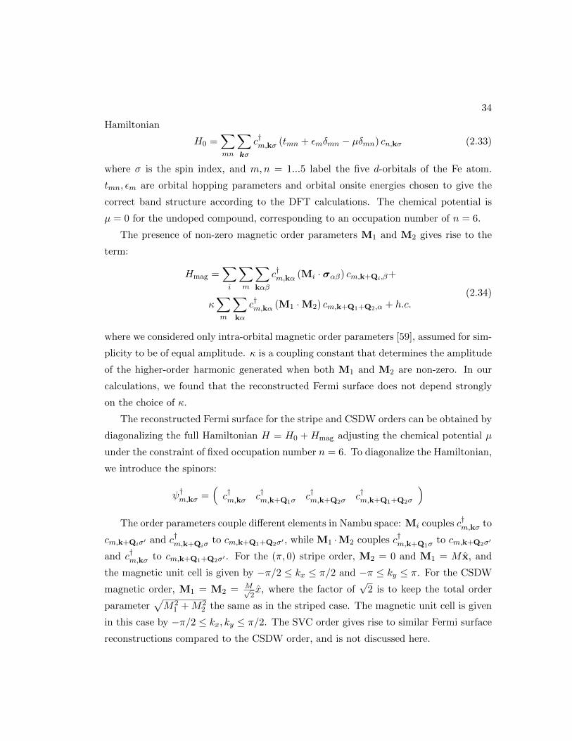
34

Hamiltonian

H0 =∑

mn

∑

kσ

c†m,kσ (tmn + εmδmn − µδmn) cn,kσ (2.33)

where σ is the spin index, and m,n = 1...5 label the five d-orbitals of the Fe atom.

tmn, εm are orbital hopping parameters and orbital onsite energies chosen to give the

correct band structure according to the DFT calculations. The chemical potential is

µ = 0 for the undoped compound, corresponding to an occupation number of n = 6.

The presence of non-zero magnetic order parameters M1 and M2 gives rise to the

term:

Hmag =∑

i

∑

m

∑

kαβ

c†m,kα (Mi · σαβ) cm,k+Qi,β+

κ∑

m

∑

kα

c†m,kα (M1 ·M2) cm,k+Q1+Q2,α + h.c.(2.34)

where we considered only intra-orbital magnetic order parameters [59], assumed for sim-

plicity to be of equal amplitude. κ is a coupling constant that determines the amplitude

of the higher-order harmonic generated when both M1 and M2 are non-zero. In our

calculations, we found that the reconstructed Fermi surface does not depend strongly

on the choice of κ.

The reconstructed Fermi surface for the stripe and CSDW orders can be obtained by

diagonalizing the full Hamiltonian H = H0 + Hmag adjusting the chemical potential µ

under the constraint of fixed occupation number n = 6. To diagonalize the Hamiltonian,

we introduce the spinors:

ψ†m,kσ =(c†m,kσ c†m,k+Q1σ

c†m,k+Q2σc†m,k+Q1+Q2σ

)

The order parameters couple different elements in Nambu space: Mi couples c†m,kσ to

cm,k+Qiσ′ and c†m,k+Qiσto cm,k+Q1+Q2σ′ , while M1 ·M2 couples c†m,k+Q1σ

to cm,k+Q2σ′

and c†m,kσ to cm,k+Q1+Q2σ′ . For the (π, 0) stripe order, M2 = 0 and M1 = M x, and

the magnetic unit cell is given by −π/2 ≤ kx ≤ π/2 and −π ≤ ky ≤ π. For the CSDW

magnetic order, M1 = M2 = M√2x, where the factor of

√2 is to keep the total order

parameter√M2

1 +M22 the same as in the striped case. The magnetic unit cell is given

in this case by −π/2 ≤ kx, ky ≤ π/2. The SVC order gives rise to similar Fermi surface

reconstructions compared to the CSDW order, and is not discussed here.

35

-π

0

π

-π 0 π

(a)

M1

M2

-π/2

0

π/2

-π/2 0 π/2

(b)

-π/2

0

π/2

-π/2 0 π/2

(c)

Figure 2.10: Reconstructed Fermi surfaces near the center of the Brillouin zone inthe presence of Q1 = (π, 0) stripe magnetic order (b) and CSDW magnetic order (c).The Fermi surface in the paramagnetic state is shown in (a), with the tight-bindingparameters of Ref. [49]. From Ref. [35].

In Fig. 2.10, we present the reconstructed Fermi surface around the center of the

magnetic Brillouin zone for both magnetic ground states. In the paramagnetic phase,

the Fermi surface consists of two concentric hole pockets at the center of the Brillouin

zone and two elliptical pockets centered at the momenta Q1 = (π, 0) and Q2 = (0, π).

In the striped state, we find that for reasonable values of the magnetic order parameter

(M ≈ 60 meV), one of the hole pockets remains unhybridized while the other hole

pocket hybridizes with the folded electron pocket, giving rise to ”Dirac cones” – the

small reconstructed pockets along the stripe modulation direction. This is in general

agreement with previous theoretical and experimental results [60, 61, 59]. On the other

hand, for the CSDW state, each of the two hole pockets hybridize with one of the

two electron pockets. As a result, there remains only small reconstructed pockets [62].

Unlike the small pockets that appear in the stripe state case, four of these pockets appear

along the Q1 + Q2 = (π, π) direction. We found that a non-zero CDW order parameter

ρQNdoes not lead to qualitative differences in the reconstructed Fermi surface.

36

2.4.2 Spin wave


A main difference between the SVC and the stripe phase is the absence of collinear

spins (see Fig. 2.3). As has been shown in Ref. [63], the number of Goldstone modes

(acousticspin waves) for collinear and non-collinear magnetic phases are different, due

to different number of broken rotational symmetry generators in the spin space. In this

section, we study in details the spin-wave spectrum of the SVC magnetic phase, and

compare it to the stripe phase.

As we are interested in the low-energy behavior, there are two alternative approaches

to compute the spin-wave spectrum: the first is by evaluating self-consistently the poles

of the spin-spin correlation function deep inside the magnetically ordered state within

the itinerant approach described in the previous section [64]. The second alternative

is to build a phenomenological localized-spin model that gives the same ground states

as the itinerant model, and then use Holstein-Primakoff (HP) bosons to compute the

spin-wave dispersion.[65, 66]. 4 Given the simplicity of the latter, we here consider

a Heisenberg model on a two-dimensional square lattice, with nearest-neighbor and

next-nearest neighbor interactions:

H = J1

∑

〈i,j〉Si · Sj + J2

∑

〈〈i,j〉〉Si · Sj −

K

S2

∑

〈i,j〉(Si · Sj)2 (2.35)

where 〈...〉 and 〈〈...〉〉 denote nearest-neighbors and next-nearest neighbors, and J1 > 0,

J2 > J1/2 are the respective antiferromagnetic exchange interactions. The biquadratic

term K selects between the stripe phase (K > 0) and the SVC phase (K < 0) in the

classical regime. We emphasize that this is a phenomenological model constructed to

describe the ground states obtained in Section II. Indeed, as discussed previously, if it

was the classical J1-J2 model, K would be restricted to small positive values only [48].

Instead, here K should be understood as a phenomenological parameter, analogous

to the parameter g calculated in Eq. (2.19). In fact, a Ginzburg-Landau expansion

of this toy Heisenberg model would result in a free energy equivalent to that of Eq.

(2.19), evidencing the fact that both models share the same low-energy properties [68].

4 To study spin-wave spectrum of the CSDW phase, we need to work with the itinerant modelrather than the J1-J2 spin Heisenberg model. This is not done here. For a more thorough investigationof magnetic excitations of the CSDW order, refer to Ref. [67].

37

A

B

A

B

A

B

A

B

zx

1 2 1 2

3 4

Figure 2.11: Magnetic unit cell for the stripe magnetic order with wavevector Q1, andSVC order with wavevectors Q1 and Q2. In the text for introducing Holstein-Primakovbosons, we used a local spin coordinate system, where the z axis is parallel to the localspin alignment. The global spin coordinate system is chosen to be that for site 1.

Therefore, the use of this localized-spin model should be understood simply as a tool

to evaluate the spin-wave spectrum, and not an implication that local moments are

necessarily present in the system. Incidentally, we note that other Heisenberg models

with ring exchange interactions can also display the SVC order [69].

We emphasize that a strict two-dimensional model does not have long-range Heisen-

berg magnetic order, according to Mermin-Wagner theorem. As a result, we assume here

that the system is formed by weakly-coupled layers. Such a small inter-layer coupling

can nevertheless be neglected in what regards the main properties of the spin-wave dis-

persions. To obtain the spin-wave spectrum of the Hamiltonian (2.35), we follow Refs.

[70, 71] and introduce locally Holstein-Primakoff (HP) bosons for each of the r spins in

a single magnetic unit cell:

S(r)z = S − a(r)†a(r)

S(r)+ =

√2S − a(r)†a(r) a(r) (2.36)

S(r)− = a(r)†

√2S − a(r)†a(r)

Here a annihilates a HP boson. Note that the spin coordinate system is defined locally,

such that the local spin is always parallel to the local +z axis, see Fig. 2.11. For

convenience, the two-dimensional lattice plane xy is chosen to be the xz spin-plane.

38

Since different types of spins within a magnetic unit cell have their own degree of

freedom, the number of HP bosons (labeled by r) is equal to the number of spins within

a magnetic unit cell. Thus, the stripe state has r = 1, 2 whereas the SVC state has

r = 1, 2, 3, 4. The Fourier transform of the HP bosons is defined as

a(r)k =

∑

i∈ra

(r)i e−ik·x

(r)i (2.37)

where i labels different magnetic unit cells, and x(r)i is the position of the r-th spin in

the i-th magnetic unit cell. For convenience, we define:

Ψ†k ≡(a

(1)†k , a

(1)−k, a

(2)†k , a

(2)−k, ...

)(2.38)

Because we are interested in the classical limit, we perform a large S expansion and

keep only terms that are quadratic in the bosonic operators. In this case, the Heisenberg

Hamiltonian can be re-expressed as:

H = H0 +1

2

∑

k

Ψ†kHkΨk (2.39)

where H0 is the classical ground state energy for a given spin configuration. The spin-

wave modes can be obtained by a generalized Bogoliubov transformation, Ψk = UkΦk.

To ensure that the transformed operators satisfy the correct bosonic commutation re-

lations, it is convenient to introduce the Bogoliubov metric:

η = diag(1,−1, 1,−1, ...) (2.40)

Then, the generalized Bogoliubov transformation satisfies:

U†k η Uk = η

U−1k

(η Hk

)Uk =

(η Hk

)diag(2.41)

The spin-wave modes are therefore the eigenvalues of η Hk.

Spin wave excitations in the stripe magnetic phase

As discussed above, the stripe phase is the ground state of the model (Eq. 2.35) for

K > 0. The spin-wave dispersion of the stripe phase was obtained previously in Refs. [72,

39

73, 74] and here we rederive the results to compare them later with the SVC case. For

concreteness, we first consider the stripe phase with ordering vector Q1 = (π, 0). As

shown in Fig. 2.11, there are two spins per magnetic unit cell, whose HP operators we

denote by a(1)k and a

(2)k . Note that, with respect to the spin coordinate system defined

on site 1, the spin on site 2 is rotated by 180, yielding:

S(2) =(−S(2)

x , S(2)y ,−S(2)

z

)(1)

(2.42)

Using the Holstein-Primakoff transformation defined in Eq. 2.38, we find that the

large-S Hamiltonian is given by:

Hk =

εk 0 0 ∆k

0 εk ∆k 0

0 ∆k εk 0

∆k 0 0 εk

(2.43)

with:

εk = 2S [(J1 − 2K) cos ky + 2J2 + 4K]

∆k = −2S (J1 + 2K + 2J2 cos ky) cos kx (2.44)

The Hamiltonian is diagonalized via the Bogoliubov transformation

Uk =

uk 0 0 vk

0 uk vk 0

0 vk uk 0

vk 0 0 uk

(2.45)

with:

u2k =

1

2

(1 +

εkωk

); v2

k =1

2

(−1 +

εkωk

); ukvk = −1

2

∆k

ωk(2.46)

yielding the doubly-degenerate eigenmode (i.e. spin-wave mode) of the bosonic system:

ωk =√ε2k −∆2

k (2.47)

The fact that there are two degenerate spin-wave modes for the stripe state is a

consequence of the fact that ωk+Q1 = ωk and also of the collinear configuration of the

40

Figure 2.12: Spin-wave dispersions for the stripe phase with ordering vector Q1 = (π, 0)(a) and Q2 = (0, π) (b). Both are doubly degenerate modes. The energies are in unitsof 4J2S and the parameters used are J1 = 0.8J2 and K = 0.1J2. From Ref. [36].

spins. The spin-wave dispersion of the stripe phase with ordering vector Q2 = (0, π)

can be calculated in the same way, yielding ωQ2 (kx, ky) = ωQ1 (ky,−kx), as expected.

In Fig. 2.12, we show the dispersion of the spin waves (Eq. 2.47) for the two types of

stripe orders in their respective magnetic Brillouin zones. The results obtained here are

in agreement with those obtained previously elsewhere [74].

Spin wave excitations in the SVC phase

The SVC phase becomes the ground state of Eq. 2.35 for K < 0. As shown in Fig. 2.11,

there are four spins per magnetic unit cell, giving rise to the HP operators a(1)k , a

(2)k ,

a(3)k , and a

(4)k . Because the spins on sites 2, 3, 4 correspond respectively to rotations of

90, 180, and 270 relative to the spin on site 1, we define the local spin coordinate

systems:

S(2) = (S(2)z , S(2)

y ,−S(2)x )(1)

S(3) = (−S(3)z , S(3)

y , S(3)x )(1)

S(4) = (−S(4)x , S(4)

y ,−S(4)z )(1) (2.48)

Introducing Ψ†k as defined in Eq. 2.38 and substituting in the Hamiltonian, we obtain

in the large-S limit:

Hk =

Ak Bk Ck Dk

Bk Ak Dk Ck

Ck Dk Ak Bk

Dk Ck Bk Ak

(2.49)

41

where we defined four 2× 2 matrices, Ak, Bk, Ck, and Dk of the form:

Ok =

(O1,k O2,k

O2,k O1,k

)(2.50)

with the matrix elements:

A1,k = 4S (J2 −K) , A2,k = −4SK

B1,k = S (J1 + 2K) cos kx, B2,k = −S (J1 − 2K) cos kx

C1,k = S (J1 + 2K) cos ky, C2,k = −S (J1 − 2K) cos ky

D1,k = 0, D2,k = −4SJ2 cos kx cos ky (2.51)

The generalized Bogoliubov transformation is given by:

Uk =

Xk Yk Zk Wk

Xk −Yk Zk −Wk

Xk Yk −Zk −Wk

Xk −Yk −Zk Wk

(2.52)

where the four 2× 2 matrices, Xk, Yk, Zk, and Wk are also of the form (2.50). For Xk,

the matrix elements are given by:

X21,k =

1

8

(1 +

εkωk

)

X22,k =

1

8

(−1 +

εkωk

)

X1,kX2,k = −1

8

∆k

ωk(2.53)

with:

εk = A1,k +B1,k + C1,k +D1,k

∆k = A2,k +B2,k + C2,k +D2,k (2.54)

and the spin-wave dispersions:

ωk =√ε2k −∆2

k (2.55)

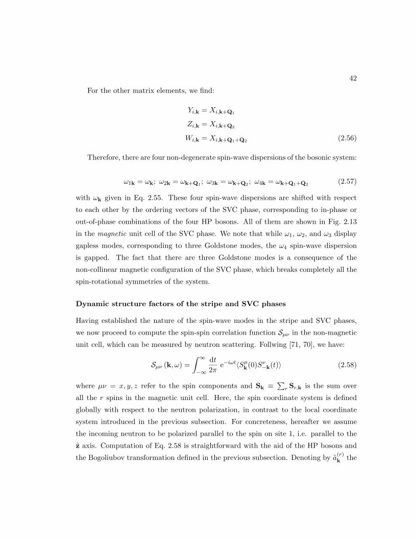
42

For the other matrix elements, we find:

Yi,k = Xi,k+Q1

Zi,k = Xi,k+Q2

Wi,k = Xi,k+Q1+Q2 (2.56)

Therefore, there are four non-degenerate spin-wave dispersions of the bosonic system:

ω1k = ωk; ω2k = ωk+Q1 ; ω3k = ωk+Q2 ; ω4k = ωk+Q1+Q2 (2.57)

with ωk given in Eq. 2.55. These four spin-wave dispersions are shifted with respect

to each other by the ordering vectors of the SVC phase, corresponding to in-phase or

out-of-phase combinations of the four HP bosons. All of them are shown in Fig. 2.13

in the magnetic unit cell of the SVC phase. We note that while ω1, ω2, and ω3 display

gapless modes, corresponding to three Goldstone modes, the ω4 spin-wave dispersion

is gapped. The fact that there are three Goldstone modes is a consequence of the

non-collinear magnetic configuration of the SVC phase, which breaks completely all the

spin-rotational symmetries of the system.

Dynamic structure factors of the stripe and SVC phases

Having established the nature of the spin-wave modes in the stripe and SVC phases,

we now proceed to compute the spin-spin correlation function Sµν in the non-magnetic

unit cell, which can be measured by neutron scattering. Follwing [71, 70], we have:

Sµν (k, ω) =

∫ ∞

−∞

dt

2πe−iωt〈Sµk(0)Sν−k(t)〉 (2.58)

where µν = x, y, z refer to the spin components and Sk ≡∑

r Sr,k is the sum over

all the r spins in the magnetic unit cell. Here, the spin coordinate system is defined

globally with respect to the neutron polarization, in contrast to the local coordinate

system introduced in the previous subsection. For concreteness, hereafter we assume

the incoming neutron to be polarized parallel to the spin on site 1, i.e. parallel to the

z axis. Computation of Eq. 2.58 is straightforward with the aid of the HP bosons and

the Bogoliubov transformation defined in the previous subsection. Denoting by a(r)k the

43

Figure 2.13: The spin-wave dispersions of the SVC order in the magnetic Brillouin zone.The four dispersions are linked by a shift of the momentum coordinate system by theSVC ordering vectors. Here, the energies are in units of 4J2S and the parameters areJ1 = 0.8J2 and K = −0.1J2. From Ref. [36].

Bogoliubov-transformed bosonic operators, the only non-zero terms, at T = 0, are those

of the form: ∫ ∞

−∞

dt

2πe−iωt

⟨a

(r)k (0) a

†(r)k (t)

⟩= δ (ω − ωr,k) (2.59)

We first consider the stripe phase with the two possible ordering vectors Q1 = (π, 0)

and Q2 = (0, π). We find that only the transverse components Sxx = Syy are non-

zero, i.e. the longitudinal component Szz and the off-diagonal components Si 6=j do not

acquire spin-wave contributions. We obtain:

SQixx (k, ω) = 2S (uk − vk)2 δ

(ω − ωQi

k

)(2.60)

where uk, vk are given by Eq. (2.46) and ωQ2

(kx,ky) = ωQ1

(−ky ,kx), with ωQ1

k given by

Eq. (2.47). The total spin-spin correlation function, S =∑

i Sii is then simply

S (k, ω) = 2Sxx (k, ω). In Fig. 2.14, we plot S(k, ω) for both the Q1 and Q2 stripe

44

phases separately, as well as for a system containing equal domains of Q1 and Q2:

Sdomain (k, ω) =1

2SQ1 (k, ω) +

1

2SQ2 (k, ω) (2.61)

The latter is the case relevant for the real systems, since twin domains are al-

ways formed in the iron pnictides. In all the plots, the delta function is replaced by

a Lorentzian with width γ = 0.05 in units of 2J2S. From the figure, we see that the

system with twin domains display anisotropic spin-wave branches emerging from the

ordering vectors Q1 = (π, 0) and Q2 = (0, π), as expected. In all cases, the structure

factor vanishes at center of the Brillouin zone, but diverges at the ordering vectors Qi.

Therefore, expanding the spin-wave dispersion around the ordering vector Qi yields (θ

denote the polar angle between k and kx):

ωk+Qi≈ 4S |k|

√(J2 +K +

J1

2

)(J2 +K ± J1

2cos 2θ

)(2.62)

which is anisotropic along the kx and ky axis, as expected. In the previous expression,

the upper (lower) sign refers to Q1 (Q2).

For the SVC phase, we find that all diagonal components Sii acquire spin-wave

contributions. This is expected since the magnetic configuration is non-collinear (see

Fig. 2.3), implying that all directions are “transverse” with respect to the sublattice 1, 3

and/or the sublattice 2, 4. In particular, we find:

Sxx (k, ω) = Szz (k, ω) = 4S (Y1,k + Y2,k)2 δ (ω − ω2,k)

+ 4S (Z1,k + Z2,k)2 δ (ω − ω3,k)

Syy (k, ω) = 16S (X1,k −X2,k)2 δ (ω − ω1,k) (2.63)

with the Bogoliubov transformation parameters and spin-wave modes defined in Eqs. 2.53

and 2.57. In Fig. 2.15, we plot these diagonal components as well as the total structure

factor S =∑

i Sii. In the latter, we observe two spin-wave branches emerging from

the ordering vectors Q1 = (π, 0) and Q2 = (0, π), in sharp contrast to the case of do-

mains of stripes, where only one spin-wave branch emerges from each ordering vector

(see Fig. 2.14). We note that, once again, the structure factor vanishes at the center

of the Brillouin zone and diverges at the magnetic ordering vectors Q1 = (π, 0) and

45

Figure 2.14: The total spin-spin structure factor S =∑

i Sii = 2Sxx for the Q1 (toppanel) and Q2 (mid panel) stripe phases. Bottom panel is the structure factor assumingequal domains of Q1 and Q2 stripes. The vertical axis is the energy measured inunits of 4J2S, whereas the horizontal axis displays momentum cuts in the Fe-square-lattice Brillouin zone. The intensity is highest at the ordering vectors Q1 and Q2. Theparameters used here are J1 = 0.8J2 and K = 0.1J2. From Ref. [36].

Q2 = (0, π). Expanding the dispersions near them, we find (recall that K < 0):

ω1,k+Q1 ≈ 4S |k|√

(J2 −K)

(J2 +

J1

2cos 2θ

)

ω2,k+Q1 ≈ 4S |k|√

(J2 −K)

(J2 +

J1

2

)

ω3,k+Q1 ≈ 8S√

(2J2 − J1) (−K) (2.64)

46

as well as:

ω1,k+Q2 ≈ 4S |k|√

(J2 −K)

(J2 −

J1

2cos 2θ

)

ω2,k+Q2 ≈ 8S√

(2J2 − J1) (−K)

ω3,k+Q2 ≈ 4S |k|√

(J2 −K)

(J2 +

J1

2

)(2.65)

Therefore, we obtain two gapless spin-wave branches emerging from each ordering

vector, as shown in Fig. 2.15, as well as one gapped spin-wave dispersion. As expected,

tetragonal symmetry is preserved by these dispersions. Interestingly, along the direction

parallel to the Qi vector, the two spin-wave velocities are equal, whereas along the

direction perpendicular to the Qi vector, they are different. In the latter case, their

ratio is given by:

c1,⊥c2,⊥

=

√2J2 + J1

2J2 − J1(2.66)

where the ⊥ sign indicates that the spin-wave velocity is measured relative to the di-

rection perpendicular to the ordering vector Qi. Interestingly, this ratio does not de-

pend on the biquadratic coupling K. These qualitative features, in principle, allow one

to experimentally distinguish, in an unambiguous way, whether the magnetic ground

state is stripe or SVC. Note that, in the SVC phase, no spin-wave modes emerge from

Q1 + Q2 = (π, π).

Continuing the investigation of the SVC phase, we find that the spin-waves also

contribute to the off-diagonal component:

Sxz (k, ω) = 4S (Y1,k + Y2,k)2 δ (ω − ω2,k)

− 4S (Z1,k + Z2,k)2 δ (ω − ω3,k) (2.67)

providing another criterion to distinguish experimentally the SVC and stripe phases via

polarized neutron scattering.

In principle, the structure factor tensor of the SVC phase can be brought in a

diagonal form if the neutron is polarized along z = (x + z) /√

2, instead of parallel to

the spin on site 1. In this new coordinate system, each of the three gapless spin-wave

47

Figure 2.15: The structure factors Sxx = Szz (top panel), Syy (mid panel) and S =∑i Sii (bottom panel) for the SVC phase. The vertical axis is the energy measured in

units of 4J2S, whereas the horizontal axis displays momentum cuts in the Fe-square-lattice Brillouin zone. The parameters used here are J1 = 0.8J2 and K = −0.1J2.Two gapless spin-wave branches emerge from the ordering vectors Q1 = (π, 0) andQ2 = (0, π), in sharp contrast to the case of domains of stripes shown in Fig. 2.14.From Ref. [36].

dispersions contribute only to one of the diagonal components, and we find:

Szz (k, ω) = 8S (Y1,k + Y2,k)2 δ (ω − ω2,k)

Sxx (k, ω) = 8S (Z1,k + Z2,k)2 δ (ω − ω3,k) (2.68)

as well as Syy = Syy.

Summary

In summary, based on the J1-J2-K spin-Heisenberg model we calculated the low-energy

spin wave excitations of both the stripe and the spin-vortex crystal phase. We showed

that due to the noncollinear magnetic structure of the SVC phase, the number of Gold-

stone modes is 3, compared to 2 in the collinear case. The results are consistent with the

results obtained in Ref. [63]. The counting of Goldstone modes can be used to uniquely

48

differentiate between collinear versus non-collinear magnetic orders. Additionally, by a

detailed calculation of the spin-spin correlation function, we showed that in the stripe

phase, there is one Goldstone mode located at the magnetic ordering wavevector Q1,

and two for the SVC case.

2.5 Conclusions

In this chapter, we investigated the nature and origin of magnetic orders in iron pnictide

materials, and proposed direct measurements of various magnetic orders based on Fermi

surface reconstruction and collective spin wave excitations.

The significance of C4 magnetic orders is two-fold. First, C4 magnetic orders can be

realized from an itinerant picture, but not from a localized J1-J2 spin-Heisenberg model.

This suggests that magnetism in iron pnictide materials are of itinerant nature, and a

result of Fermi surface instability. This is different than that in cuprate superconduc-

tors. Second, C4 magnetism competes more strongly with superconductivity than C2

magnetism. In a collaborative work [37], we showed theoretically that superconducting

transition temperature is reduced in the coexisting phase of superconductivity and C4

magnetism. This was also observed experimentally in Ba1−xKxFe2As2 [29].

We also proposed experimental signatures based on Fermi surface reconstruction

and collective spin wave excitations. These properties are direct manifestations of the

electronic order, rather than relying on magnetoelastic coupling, therefore, they can be

used to uniquely determine the nature of the magnetic orders, being stripe, SVC or

CSDW magnetism.

Since in iron pnictide materials, both superconductivity and magnetism emerge due

to Fermi surface instability, their interplay needs to be placed on an equivalent footing,

contrasted to the spin-fermion model described in Ch. 4 Sec. 4.2, where magnetism is

assumed to come from physics beyond the Fermi surface. A purely electronic model

which captures both physics is described by the Hamiltonian:

H =∑

i=c,d;σ

(εk − µ)ψ†ikσψikσ − U∑

r

(ψ†cα~σαβψ

†dβ + h.c.

)2(2.69)

where c and d are electronic annihilation operators for two electronic bands (see Ch. 4

Sec. 4.2 for details). This model can be studied using the sign-problem-free Quantum

49

Monte Carlo method discussed in appendix A, with preliminary results suggesting that

both superconductivity and magnetic order can be found by in the T,U parameter

space.

Chapter 3

Origin of electronic nematicity in

iron-based superconductors and

manifestations in Scanning

Tunneling Spectroscopy

3.1 Introduction

As was discussed in Ch. 1 and Ch. 2, in most iron pnictide superconductors, there is

a structural phase transition at TS where the square lattice symmetry (C4) is broken

down to orthorhombic (C2), followed by a magnetic phase transition at TN into a stripe

magnetic phase, where the spins are ferromagnetically aligned along one of the Fe-

Fe bond directions, and antiferromagnetically aligned along the other. Fig. 3.1 is a

schematic phase diagram of the iron pnictide materials[21]. While in some materials

such as (Ba1−xKx)Fe2As2, the two transition temperatures coincide [9], other materials

such as Ba(Fe1−xCox)2As2 exhibit an intermediate nematic phase, where the square

lattice symmetry is broken while long range magnetic order is absent[17]. The two

transition temperatures follow each other closely even in the doped materials, suggesting

the intimate relationips between the nematic and magnetic phases.

Although the nematic order manifests itself in both lattice and electronic degrees of

50

51 Report on Progress

2

features shown in figure 1 (for reviews, see [3–6]). Specifically, the parent compounds of most (but not all) FeSC are magnetically ordered metals. In most cases, the magnetic order is of a stripe type—i.e. spins are ferromagnetically aligned in one direction in the Fe plane and antiferromagn etically aligned in the other. This is usually known as the 0, , 0( )/( )π π spin-density wave (SDW) state. Upon hole or electron doping, or upon substitution of one pnictide atom by another, magnetic order goes away and a dome of superconductivity emerges. In addition, there is a region on the phase diagram where the system displays nematic order, in which the C4 lattice rotation symmetry is spontaneously broken (C4 is the point group symmetry associated with a square, whereas C2 is the point group symmetry associated with a rec-tangle). The nematic order naturally coexists with the stripe magnetic order and in some systems also coexists with super-conductivity [7].

Despite the similarities in their phase diagrams, there are important differences between the cuprates and FeSC. The most pronounced difference is that the low-energy electronic states of the cuprates arise from Cu2+ , which is in a 3d 9 elec-tronic configuration, while in the FeSC the low-energy states arise from Fe2+ , which is in a 3d 6 configuration. One imme-diate consequence of this difference is that parent compounds of the cuprates are Mott insulators, while parent compounds of FeSC are metals. The relevance of metallicity of FeSC has been discussed in earlier reviews and we will not dwell on this [8–10]. In this review we focus on another immediate conse-quence of the difference between 3d 9 and 3d 6 electronic con-figurations, namely the fact that the 3d 6 configuration involves five 3d orbitals – dxz, dyz, dxy, dx y2 2− , and d z r3 2 2− , while 3d9 configuration contains a single dx y2 2− orbital. This brings important consequences for microscopic models constructed to describe 3d 9 and 3d 6 systems.

In a free space, the five 3d orbitals are all degenerate. In a crystalline environment the degeneracy is lifted, and the energy levels are split into two subsets, t2g and eg, with three and two orbitals, respectively: dxz, dyz, and dxy for t2g and dx y2 2− and d z r3 2 2− for eg (the subscript g implies that the states are sym-metric under inversion). In some multi-orbital systems, such as the manganites (3d 5) and the cobaltates (3d 7), the crystal-field splitting is large, and this allows one to focus on only one subset. In FeSC the situation is more subtle because the As/Se positions alternate between the ones above and below the center of the Fe plaquettes, as shown in figure 2. As pointed

out in [11], because of such puckering of the As/Se atoms, the crystalline environ ment experienced by Fe atoms is somewhat in between a tetrahedral one, in which the energy of the t2g orbitals is higher than that of the eg orbitals, and a tetrago-nal one, in which the energy of the t2g orbitals is lower (see figure 2 and [11]). As a result, the crystal splitting between the orbitals is weakened in FeSC and, consequently, all five d-orbitals must be kept in the kinetic energy Hamiltonian:

t d d .ij

i j i j0,

, , ,∑ ∑=µν σ

µ ν µ σ ν σH † (1)

Here d i,†µ σ creates an electron at site i and orbital µ

( 1, ..., 5µ = ) with spin σ, and t i j,µ ν are hopping amplitudes. The diagonal terms describe the dispersions of electrons from separate orbitals, whereas the non-diagonal terms account for the hopping from one orbital to the other. The latter give rise to hybridization of the eigenstates from different orbitals. The

stripeSDW

nematic

temperature

1-x x 2 2

SCSC

1-x x 2 2

Figure 1. Schematic phase diagram of electron-doped (Co-doped) and hole-doped (K-doped) BaFe2As2, displaying stripe spin-density wave (SDW) order, nematic order, and superconductivity (SC).

Figure 2. (upper panel) Schematic crystal structure of an FeAs or FeSe plane, displaying the puckering of the As/Se atoms above and below the square Fe plane. (lower panel) The crystal field splittings of the 3d eg (red) and t2g (blue) orbitals from a tetragonal and a tetrahedral environment (a similar figure was published in [11]).

Rep. Prog. Phys. 80 (2017) 014503

Figure 3.1: Schematic phase diagram of electron-doped (Co-doped) and hole-doped (K-doped) BaFe2As2, displaying stripe spin-density wave (SDW) order, nematic order, andsuperconductivity (SC). Taken from Ref. [21].

freedom, various experiments have shown that the nematic order is driven by electronic

correlations[75, 76]. For example, in the Ba(Fe1−xCox)2As2 compound, the observed

anisotropy is much more pronounced in the electrical resisitivity than in the orthorhom-

bic distortion of the lattice[75, 30]. A more definitive evidence is given by Ref. [76], which

showed that TS marks a divergence of the electronic nematic susceptibility.

There are two main scenarios where electronic nematicity can emerge in the iron

pnictide materials, namely, the orbital scenario [77] and the magnetic scenario [74, 44].

In the orbital scenario, the nematic order is due to the electronic system developing

an “orbital order” at TS , where the occupation number of the Fe dxz and dyz orbitals

becomes different. The electronic nematic order can be defined by the charge imbalance

between the dxz and dyz orbitals: φ ∝ 〈nxz − nyz〉, where nxz/yz is the occupation

number in the corresponding electronic orbital, and 〈· · · 〉 denotes thermal averaging.

In this scenario, electronic nematicity and stripe magnetism do not necessarily come

together. This has been used to explain the absence of long range magnetic order in

the iron chalcogenide compound FeSe, see Fig. 1.5.

In the magnetic scenario, the nematic order is driven by strong magnetic fluctuations.

Following the discussion in Ch. 2, the magnetic order in most iron pnictide materials

can be described by two magnetic order parameters M1 and M2, with wavevectors

52

TS

hM1i = hM2i = 0

hM21 M2

2i 6= 0

hM1i = hM2i = 0

hM21i = hM2

2ihM1i 6= 0

orhM2i 6= 0

TN

Figure 3.2: Magnetic scenario. The melting of long range stripe magnetic order goesin two steps. First, spin rotational symmetry is restored at TN . Then, the tetragonalsymmetry is restored at TS .

Q1 = (π, 0) and Q2 = (0, π) respectively. In the stripe magnetic phase, either M1 or M2

becomes non-zero, which simultaneously breaks the square lattice symmetry (C4) down

to orthorhombic (C2). If magnetic fluctuations are taken into account, upon raising

temperature, the “melting” of the stripe magnetic order can occur in two steps (Here I

use the stripe order with M1 6= 0 to illustrate the idea): At a temperature TN , the spin

rotational symmetry is restored, and the long range magnetic order is lost. However, the

magnetic fluctuations at Q1 and Q2 can still be inequivalent, 〈M21〉 6= 〈M2

2〉. Therefore,

the nematic order parameter φ ∝ 〈M21 −M2

2〉 remains non-zero. Only at a higher

temperature TS does the system recover the C4 symmetry. Fig. 3.2 shows schematically

the magnetic scenario. This scenario is very successful at explaining why the nematic

phase transition temperature follows the magnetic transition temperature, observed in

most iron pnictide materials.

It is important to understand the origin of the electronic nematicity. Not only

does it encode the dominant low-energy electronic correlations, but it also constrains

the appropriate low-energy effective descriptions of the electronic phase diagram of iron

pnictide superconductors. This is a difficult question to answer, because the orbital order

and the spin-nematic order breaks the same square lattice symmetry, and therefore will

always appear together[78]. On the other hand, the orbital order scenario and the spin-

nematic scenario can have quite different experimental manifestations. In particular, the

53

feedback of nematicity on the electronic and magnetic spectrum can be quite different

for these two scenarios [78]. In addition, recent theoretical studies have shown that the

two scenarios have opposite effects on the electrical resistivity anisotropy[79].

In this chapter, I will focus on the magnetic scenario. I will first discuss how the

electronic nematic order can emerge due to strong magnetic fluctuations. Motivated by

recent results on the spectroscopic manifestations of the electronic nematic order [80], I

studied the effects of strong stripe antiferromagnetic fluctuations on the local electronic

density of states near an impurity. I will show that the spectroscopic results are fully

consistent with the predictions from the magnetic scenario.

3.2 Nematicity as a vestigial order to stripe magnetism

This section reproduces previous results published in Ref. [44].

As shown in Ch. 2, the onset of magnetic order in the iron pnictide materials can

be described using a Ginzburg-Landau free energy which preserves the spin rotational

symmetry and the square lattice symmetry (see also Eq. 2.5):

F =r0

2(M2

1 + M22) +

u

4(M2

1 + M22)2 − g

4(M2

1 −M22)2 + w(M1 ·M2)2 (3.1)

The mean-field phase diagram, obtained by minimizing the free energy, has been pre-

sented in Fig. 2.4. In particular, the stripe magnetic order becomes the ground state

if g > min0,−w. As was shown in Ch. 2, w can become non-zero when residual

electronic interactions or Neel-type antiferromagnetic fluctuations are considered. For

simplicity we set w = 0. As a result, the criterion for stripe magnetic order becomes

g > 0.

In the mean-field approximation, both the square lattice symmetry and the spin

rotational symmetry are broken at the same temperature, therefore TS = TN . While

this is true for some iron pnictide materials such as Ba1−xKxFe2As2, in many other

systems they appear as split phase transitions. Theoretically, to see how split nematic

and magnetic phase transitions occur, one needs to consider the effects of magnetic

fluctuations [44]. We can write down the effective bosonic action for the magnetic order

54

parameters M1,M2:

Seff =1

2

∫

qχ−1q (M1q ·M1−q + M2q ·M2−q) +

1

4

∫

x

[u(M2

1 + M22

)2 − g(M2

1 −M22

)2]

(3.2)

Here q ≡ (q, iωn), and x ≡ (x, τ). We used the notation:∫q ≡

∑n

∫q, and

∫x ≡∫ 1/T

0 dτ∫x.

The non-interacting magnetic fluctuations are characterized by the propagator (for

small momentum and frequency):

χ−1q ≈ r0 + q2 + γ|ωn| (3.3)

where r0 ∝ T−T (0)N , and T

(0)N is the mean-field magnetic transition temperature. γ is the

Landau damping parameter, describing the decay of low-energy magnetic fluctuations

into electron-hole pairs near the Fermi surface. The Landau damping parameter can be

obtained from microscopic electronic models (e.g., Ref. [33, 35]) following the standard

Hertz-Millis approach[22, 23, 44]. See also Sec. 4.2.

The partition function is given by Z =∫D[M1,M2] exp(−Seff). To study the effects

of magnetic fluctuations, we introduce two Hubbard-Stratonovich fields ψ and φ to

decouple the quartic interactions:1

exp(−Seff) =

∫D[ψ, φ] exp

ψ2

4uT− φ2

4gT− 1

2

∫

x

[ψ(M2

1 + M22

)+ φ

(M2

1 −M22

)]

(3.4)

Variation with respect to ψ, φ gives:

ψ = u〈M21 + M2

2〉; φ = g〈M21 −M2

2〉 (3.5)

As a result, ψ and φ describe the Gaussian magnetic fluctuations and the nematic order

parameter respectively. In the absence of long-range magnetic order, 〈Mi〉 = 0, and

the Gaussian magnetic fluctuations can be integrated out to give an effective action for

ψ, φ :

S = −(r − r0)2

4uT+

φ2

4gT+N

2

∫

qln[(r + q2 + γ|ωn|)2 − φ2

](3.6)

1 Here we work in the normal state before magnetic order condenses. For a treatment of the stripemagnetic phase, see Ref. [44].

55

where N is the number of spin components, and r ≡ r0 + ψ. We treat 1/N as a small

parameter, and in the large-N limit, the action can be solved using the saddle point

approximation:

r − r0

2u=

∫

q

r + q2 + γ|ωn|(r + q2 + γ|ωn|)2 − φ2

φ

2g=

∫

q

φ

(r + q2 + γ|ωn|)2 − φ2

(3.7)

where x denotes x·(TN). We can also define the magnetic correlation lengths associated

with the magnetic order parameters Mi=1,2: ξ2i ≡ (r ± φ)−1. In the nematic phase,

φ 6= 0, and the magnetic fluctuations become inequivalent ξ1 6= ξ2. The magnetic phase

transition temperature is determined by the criterion rc = |φ|.The nature of the nematic and magnetic phase transitions can be determined by

solving the coupled saddle point equations Eq. 3.7. To see this, we show one example,

where we consider a two-dimensional system at temperatures such that Tγ >> Λ2,

where Λ is the upper momentum cutoff. In this limit, only the lowest Matsubara

frequency term is relevant, and Eq. 3.7 can be simplified to be [44]:

r0 = r +u

4πln(r2 − φ2)

φ =g

4πlnr + φ

r − φr0 ≡ r0 +

u

2πln Λ

(3.8)

The second equation gives r = φ coth(2πφ/g). Substituting into the first equation:

r0 = φ coth2πφ

g+

u

2πln

(φ/ sinh

2πφ

g

)(3.9)

By rescaling the fields: φ∗ ≡ 2πφ/g, ¯r0 ≡ 2πr0/g, and defining a dimensionless ratio

α ≡ u/g, we obtain:

¯r0 = φ∗ cothφ∗ + α ln

(φ∗

sinhφ∗

)(3.10)

Fig. 3.3 shows the temperature evolution (¯r0) of the nematic order parameter for α = 1.5

and α = 2.5 respectively[44]. For α > 2, the nematic phase transition is second order,

where upon decreasing temperature (¯r0), the first solution is φ∗ = 0+. For α < 2,

the nematic phase transition becomes first order, marked by a finite jump of the order

parameter, i.e., the first solution is at φ∗ = φ∗0 6= 0.

56FERNANDES, CHUBUKOV, KNOLLE, EREMIN, AND SCHMALIAN PHYSICAL REVIEW B 85, 024534 (2012)

2.5=

*

0

r0

2 4 6

1.0

0.5

8

1.5

-0.5

-1.01.5=

FIG. 3. (Color online) ¯r0 as the function of the Ising-nematicorder parameter φ∗ = 2φ/g for two representative values 1 < α < 2(blue/dark line) and α > 2 (orange/light line). The value of φ∗ atwhich the solution first appears upon decreasing ¯r0 sets the type ofthe nematic transition. For α > 2, the solution first emerges at φ∗ = 0,and the transition is second order. For 1 < α < 2, ¯r0 is nonmonotonicfunction of φ∗ and the solution first emerges at a nonzero φ∗. Thenematic transition then becomes first order.

where φ∗ = 2φ/g, ¯r0 = 2r0/g − α ln(g/2), and α = u/g [seeEq. (21)].

Recall that the original model is constrained to u > g, i.e.,α > 1. The variable ¯r0 decreases with decreasing T , since itonly differs by a constant and by an overall factor from r0.The leading instability of the system upon decreasing T isinto a state with φ∗ corresponding to the maximum of theleft-hand side of Eq. (23). A simple analysis shows that themaximum is at φ∗ = 0 for α ! 2 and at a finite φ∗ for 1 < α <2 (see Fig. 3). The implication is that, for α ! 2, the systemundergoes a second-order Ising-nematic transition at ¯rcr

0 = 1(r = g/2), while for 1 < α < 2, the Ising-nematic transitionbecomes first order and the solution for φ∗ first appears at alarger ¯r0 = ¯rmax

0 (see Figs. 3 and 4). The value φ∗cr at which the

left-hand side of Eq. (23) has a maximum gradually increasesas α decreases, approaching infinity as α → 1.

0φ

S (φ )

1 2 3 4 51.2

1.6

2.0

2.4

eff

*

*

=1.21

=1.0

FIG. 4. (Color online) The effective action Seff [α,φ∗, ¯r0] fromEq. (25) as a function of φ∗ for α = 1.5 and several ¯r0. Theevolution of Seff is typical of a first-order phase transition. Atlarge ¯r0, Seff [1.5,φ∗, ¯r0] monotonically increases with increasingφ∗. At ¯rmax

0 = 1.21, the effective action develops an inflection point(black/dark solid curve), which at smaller ¯r0 splits into a maximumand a minimum. At ¯rcr

0 = 1.15, the values of Seff at φ∗ = 0 and at thelocal minimum at finite φ∗ become equal (black dotted curve), andthe system undergoes a first-order Ising-nematic transition. The localminimum in Seff at φ∗ = 0 survives down to ¯rmin

0 = 1 (blue/light graydotted curve).

The actual ¯rcr0 at which the first-order Ising-nematic

transition occurs is somewhat smaller than ¯rmax0 because at

¯rmax0 the effective action Seff only develops a local minimum

at a nonzero φ∗cr. The actual transition occurs when the value

of the effective action at the local minimum becomes equalto Seff(φ∗ = 0). To obtain ¯rcr

0 , we then need to evaluate theeffective action at both minima φ∗ = 0 and φ∗ = 0, and find¯rcr

0 at which the two terms become equal. For better clarity, wecompute Seff not only at the extrema [when the self-consistentequations (22) are valid], but for arbitrary φ∗ at a given ¯r0.To do this, we solve the equation ∂Seff/∂ψ = 0 to obtainr(α,φ∗, ¯r0), substitute it back into the effective action andobtain Seff[α,φ∗, ¯r0]. Carrying out the calculations, we obtain,neglecting a constant term,

Seff[α,φ∗, ¯r0] = g

8Seff[α,φ∗, ¯r0], (24)

where

Seff[α,φ∗, ¯r0] = (φ∗)2 + r∗2 − ln[(r∗)2 − (φ∗)2]

− α

4ln2[(r∗)2 − (φ∗)2] − φ∗ ln

!r∗ + φ∗

r∗ − φ∗

"

(25)

and r∗ = r∗(φ∗,α, ¯r0) is the solution of the equation

r∗ + α

2ln[(r∗)2 − (φ∗)2] = ¯r0. (26)

In Fig. 4, we plot Seff[α,φ∗, ¯r0] for α = 1.5 as a function ofφ∗ for several values of ¯r0. We see that for ¯r0 > 1.21, Seff hasa minimum only at φ∗ = 0, and Seff[1.5,φ∗, ¯r0] monotonicallyincreases with increasing φ∗. However, once ¯r0 becomessmaller than ¯rmax

0 , which for this value of α is ¯rmax0 = 1.21,

the function Seff[1.5,φ∗, ¯r0] develops an inflection point atφ∗

cr ≈ 2.72. At smaller ¯r0, this inflection point gradually splitsinto a maximum at φ < φ∗

cr and a minimum at φ > φ∗cr. At

¯rcr0 = 1.15, the values of Seff at φ∗ = 0 and at the local

minimum φ∗ = 0 become equal, and the system undergoes afirst-order Ising-nematic transition. The local minimum of Seffat φ∗ = 0 survives down to ¯rmin

0 = 1. Below this temperature,the effective action has only one minimum at a finite φ∗.

The jump in φ at the first-order transition affects the suscep-tibilities associated with the two magnetic order parameters%X and %Y , which become nonequivalent once φ becomesfinite, see Eq. (20). This implies that the static susceptibilityand the magnetic correlation length change discontinuously atthe first-order Ising transition, even though there is no magneticinstability [the value to which φ jumps is always smaller thanr , see the second equation in Eq. (22)]. Actually, as we alreadymentioned, magnetic order never emerges for d = 2 at a finitetemperature, so Z2 is the only symmetry that gets broken.

To obtain the phase diagram in the (α, ¯r0) plane, we need toanalyze the behavior of the system once the Ising order sets in.We found that the Ising-nematic order parameter continuouslyincreases with decreasing ¯r0 for all α > 1, implying that thereis no other first-order transition line in the phase diagrambesides the one at which the Ising-nematic order develops.The phase diagram is presented in Fig. 5. The upper spinodalin this figure corresponds to rmax

0 where a local minimum of Seffappears at φ∗ = 0, and the lower spinodal refers to rmin

0 whereφ∗ = 0 ceases to be a local minimum of Seff . A first-order

024534-8

Figure 3.3: Temperature evolution of the nematic order parameter for u/g = 2.5(orange) and u/g = 1.5 (blue) respectively. The nematic phase transition is secondorder for u/g = 2.5, and first order for u/g = 1.5. The first order transition is markedby a finite jump of the nematic order parameter at the transition temperature. Takenfrom Ref. [44].

Note that in two space dimensions, there is no magnetic phase transition at a finite

temperature. This is due to the Mermin-Wagner theorem, which states that there is

no continuous symmetry breaking in two dimensions. This can easily be seen from the

saddle point equations, in that r = φ (meaning a divergent magnetic correlation length

ξ2 = 1/(r − φ)) can never be satisfied.

3.3 Spectroscopic manifestations of electronic nematic or-

der driven by magnetic fluctuations

Having understood how electronic nematic order can emerge in the magnetic scenario,

we proceed to look at its experimental manifestations. In particular, we want to under-

stand the differences between the magnetic and the orbital scenario.

As discussed previously, in these two scenarios, the effects of electronic nematic order

on the low-energy electronic spectrum are quite different[21]. For the magnetic scenario,

the nematic order is accompanied by large stripe-like antiferromagnetic fluctuations,

which may even open a “pseudogap” near the Fermi level. In the orbital scenario,

the key effect is a Pomeranchuk distortion of the Fermi surface induced by orbital

57

polarization[77].

Experimentally, scanning tunneling microscopy (STM) provides a direct visualiza-

tion of the low-energy electronic properties. The key quantity measured in STM is the

local tunneling conductance at a given voltage bias eV . It can be shown that the tun-

neling conductance is proportional to the local electronic density of states n(r, ω = eV )

(LDOS), given by the imaginary part of the momentum-integrated one-particle Green’s

function:

n(r, ω) = − 1

πV

∫

k1,k2

exp[i(k1 − k2) · r]ImG

(k1 + k2

2,k1 − k2;ω + iδ

)(3.11)

Here δ is the quasiparticle decay rate, and V is the volume.

For translationally invariant systems, the electronic Green’s function depends only

on the center of mass momentum: k1 = k2, and the LDOS is spatially homogeneous.

In the presence of an impurity, the translational symmetry is broken, and interference

patterns appear. In particular, for a weak non-magnetic point-like impurity potential

described as V (r) = −αδ(r), the LDOS can be calculated using the Born approximation:

n(r, ω) = n0(ω) + δn(r, ω)

δn(r, ω) = αImχ(r, ω)(3.12)

Here χ(r, ω) ∝∫k1,k2

exp[i(k1−k2) ·r]G0(ω+ iδ,k1)G0(ω+ iδ,k2), where G0 is the elec-

tronic Green’s function unrenormalized by impurity scattering.2 As a result, the LDOS

near an impurity is sensitive to various electronic correlations, encoded in the electronic

Green’s functions. The quasiparticle interference patterns |δn(q, ω)| (QPI), defined as

the absolute Fourier transform of the LDOS, are intimately related to properties of the

Fermi surface.

The spectroscopic patterns (both LDOS and QPI) as measured by STM are great

tools to study electronic nematicity. In particular, by comparing the patterns in the

nematic phase and in the stripe magnetic phase, we can infer the origin of nematic order

in iron pnictide compounds.

In this section, I will discuss a collaborative work on the scanning tunneling spec-

troscopy measurements of a typical iron pnictide compound NaFeAs. This work has

2 A more rigorous analysis of the LDOS near a non-magnetic impurity is done later.

58

4

still open question. In the present system, breakdownof the linear dependent susceptibility in the overdopedregion coinciding with disappearance of superconductiv-ity seems to suggest the association between temperaturelinear dependence of the susceptibility and superconduc-tivity.

FIG. 5: Phase diagram of NaFe1−xCoxAs. Ts, TSDW and Tc

are determined from the resistivity in Fig. 2 and its inset.susceptibility in Fig. 3 and Fig. 4 give almost the same valuefor Ts, TSDW and Tc.

Based on TS, TSDW and Tc inferred from the resis-tivity and magnetic susceptibility, the phase diagram ofNaFe1−xCoxAs system is established from the measure-ments on single crystals, as shown in Fig. 5. The grad-ual destruction of magnetism and enhancement of su-perconductivity (rise of Tc and superconductive shieldingfraction) were observed with increasing Co doping level.A dome-shaped Tc vs. x relationship can be observed.Optimal Tc was obtained around x = 0.028 and furtherCo doping suppressed superconductivity. Tc goes to zeroaround x = 0.109. This phase diagram is quite similar tothose of 122 and 1111 systems except for that the startingcompound of the present system is superconducting. Inaddition, the optimal Tc can be achieved by about 2.8%Co doping in NaFe1−xCoxAs, much less than ∼7% Co inBa(Fe1−xCox)2As2 system.29,30 From this point of view,the phase diagram of NaFe1−xCoxAs is more similar tothat of Ba(Fe1−xNix)2As2 system,31 in which the opti-mal doping is reached at 4.6%, far from that of ∼7% inBa(Fe1−xCox)2As2.

Figure 6 displays the temperature dependence of thelow-temperature specific heat (plotted as Cp/T ) for theunderdoped and heavily overdoped crystals. The specificheat for the undoped samples shown in Fig. 6(a) ex-hibit two anomalies corresponding to the structural andSDW transitions, respectively. The TS and TSDW arewell consistent with those determined from resistivity inthe inset of Fig. 2. No anomaly corresponding to thesuperconducting transition can be observed in the spe-cific heat for the undoped sample, which could be due to

FIG. 6: (a): Temperature dependence of low-temperaturespecific heat (Cp/T ) for underdoped and heavily overdopedNaFe1−xCoxAs crystals. The arrows points to the anomaliesin the specific heat. (b): The inset shows the derivative ofspecific heat for the crystal with x = 0.014, where structural,SDW and superconducting transitions can be clearly recog-nized from the dips. (c): Specific heat as a function of temper-ature for the optimally-doped and overdoped superconduct-ing NaFe1−xCoxAs crystals. The blue line is the fitting of thespecific heat between 20 - 40 K by using Cp = Cen+Clattice.(d): Electronic specific heat Ce/T (by subtracting the lat-tice contribution from Cp/T ) as function of temperature forthe optimally doped crystal, where the dashed line representsthe normal-state electronic contribution, γn = 10.1 mJ mol−1

K−2.

Figure 3.4: Phase diagram of NaFe1−xCoxAs. The colors refer to the nematic phase(green), the stripe magnetic phase (cyan, also labeled as SDW), and the superconductingphase (yellow). From Ref. [82].

been submitted, and is listed in Ref. [81]. The experimental part of the work is led by

Prof. Abhay Pasupathy’s group from Columbia University, while I led the theoretical

part.

3.3.1 Experimental results

NaFeAs is a typical material of the 111 family of iron pnictide superconductors. The

parent compound has two known phase transitions: a structural phase transition at

TS = 52K which breaks the lattice tetragonal symmetry (C4) down to orthorhombic

(C2), and a magnetic phase transition at TN = 41K into the stripe magnetic phase.

Superconductivity is achieved by Cobalt doping, i.e., NaFe1−xCoxAs, with a maximum

Tc = 20K at x ≈ 0.028. Fig. 3.4 shows the phase diagram obtained from resistivity and

susceptibility measurements[82].

Ref. [81] performed spectroscopic studies of NaFe1−xCoxAs for a variety of temper-

atures and dopings. Here I describe the two main results.

59

a

b

a

b

-200VLow High Low High Low High Low High

+200V

a

b

c

d

e

f

g

h


+200V

a

b

c

d

e

f

g

h

(a) (b)

(c) (d)

FigureS2:a,~100nmrealspacespectroscopicimagetakeat10meVandat26K.Inset8.3nmimageshowingtheaverageofallthedefects in imagea.b, Fourier transformof real space imagea from–π/2a0 toπ/2a0with inset showing the resultingdifferenceplot.c,Fouriertransformofaveragedefectimageininsetafrom–π/2a0toπ/2a0withinsetshowingtheresultingdifferenceplot.ThetheoryforQPIthatwe(andothers)usereferstothescatteringpatternink-space(orrealspace) generatedby a single impurity, and thus the true comparison shouldbemade to theaveragedefectFT.Indeed,thelowtemperatureQPIfromtheory(Fig.S3a)matchesquitewellwiththesingle-defectexperimentalQPIpattern(Fig.S3b).Thetheorycalculationisperformedfor amodel asdescribedabovewithparameters!!! = 0 and!!"# = 0.1. Thebrightpointsalongtheqydirections(greenarrowsinFig.S3a-b)aswellastheouterfeaturesthatrunparallelto the center bright points (purple arrow in Fig. S3a-b) are both reproduced in theory. Thecenter bright points along the qy direction (green arrow Fig. S3a-b) have a slightly differentscatteringvectorslengthswiththeexperimenthavingasmallervectorlengthwhencomparedto theory, fallingwithina .03π/a0 rangeof eachother. Theouter features (purplearrowFig.S3a-b)arefatherfromthecenterinqxthenwhatisseeninexperiment,fallingwithina.1π/a0range.Whiletheorydoesn’tcaptureallthedetailsseeninexperimentalQPI,itindeedcapturesthe import scattering vectors from the band structure near the Fermi level as discussed ingreaterdetailinref.[1].

(a) (b)a

b

Figure 3.5: LDOS and QPI in the stripe magnetic phase, obtained at 26K. (a) LDOS ina 100nm×100nm real space image at bias voltage 10meV. Inset is the extracted LDOSnear a single impurity. (b) QPI plotted for kx, ky ∈ (−π/2, π/2). Inset is the QPI inthe normal state. The Fe-Fe bond directions are labeled by a and b, where a denotesthe stripe magnetic ordering direction. The figure is adapted from Ref. [81].

LDOS and QPI in the stripe magnetic phase

Fig. 3.5(a) shows the LDOS in the stripe magnetic phase (T = 26K). In the LDOS

map, the square lattice symmetry is broken down to orthorhombic. The patterns near

a single impurity are extracted and shown in the inset. It displays two bright lobes

along the magnetic ordering wavevector direction, with a separation of about 10 lattice

constants. Fig. 3.5(b) shows the QPI, defined as the absolute Fourier transformation of

the LDOS near a single impurity. Notably, the patterns exhibit a three-stripe structure

along the magnetic ordering wavevector. This is to be contrasted with the normal state,

which shows an isotropic “blob”, as depicted in the inset.

LDOS and QPI in the nematic phase

Fig. 3.6 shows the LDOS and QPI in the nematic phase. The results are obtained in

the normal state (T = 54K) by applying a uniaxial strain. Both the LDOS and QPI

patterns are quite similar to the stripe magnetic phase.

60-200V

Low High Low High Low High Low High

+200V

a

b

c

d

e

f

g

h


+200V

a

b

c

d

e

f

g

h(a) (b)

ab

a

b

Figure 3.6: LDOS and QPI in the nematic phase, obtained from the normal state(54K) subject to an uniaxial strain. The Fe-Fe bond directions are labeled by a and b,where a denotes the stripe magnetic ordering direction. Different than the 26K datapresented in Fig. 3.5, the LDOS near a single impurity is difficult to extract. As a result,the QPI is obtained by Fourier transforming the entire LDOS image. The differencecompared to Fig. 3.5 is the presence of a bright peak at Brillouin zone center. This isdue to averaging of impurities, and not a feature of the electronic properties. The figureis adapted from Ref. [81].

Temperature evolution of electronic anisotropy

The degree of electronic anisotropy can be quantified by an anisotropy parameter η,

defined as the ratio between the absolute difference in the LDOS near a single impurity

over the absolute LDOS intensity:

η ≡∑

r |n(r, eV )− n(r, eV )|∑r |n(r, eV )| (3.13)

Here r ≡ (y,−x) is the 90-degree rotation with respect to r. Fig. 3.7 shows the

temperature evolution of the anisotropy parameter (red dots). The sharp increase of

the electronic anisotropy coincides with the onset of long range stripe magnetic order.

3.3.2 Theoretical analysis

This subsection is written based on the supplementary material to Ref. [81].

In the earlier section, I presented the spectroscopic results of NaFeAs, focusing on

the measurement of the electronic anisotropy in the nematic and magnetic phases. Can

these results be explained by a magnetic origin of the electronic nematicity?

61

10 20 30 40 50 60 70

.2

.4

.6

.8

1

Aniso

tropy

Par

amet

er

Temperature (K)

34K 38K 42K

48K 52K

28K

80

no coh fac

with coh fac

experiment

only coh fac

ba c d

e g

TSDW

TS

TN

Figure 3.7: Temperature evolution of the anisotropy parameter. The nematic andmagnetic phase transitions are labeled by TS and TN respectively. Blue, orange andgreen lines are theoretical calculations. The orange line is obtained by neglecting theeffect of coherence factors due to Brillouin zone folding, but the effects of Fermi surface(FS) reconstruction (namely, poles of electronic Green’s function) are included. Thegreen line neglects FS reconstruction, but considers coherence factor effects. Blue lineincludes both. Figure is adapted from Ref. [81].

As discussed in the beginning of this section, the spectroscopic images encode the

low-energy electronic properties. In the stripe magnetic phase, an energy gap opens near

the Fermi surface. The three-stripe structure observed in the QPI (Fig. 3.5) should

be manifestations of the Fermi surface (FS) reconstruction. On the other hand, the

nematic phase does not have long range magnetic order, and therefore there is no FS

reconstruction. However, in the magnetic scenario, the nematic phase is accompanied

by large-amplitude stripe antiferromagnetic fluctuations [21]. The magnetic fluctuations

strongly renormalize the electronic Green’s function, which can be incorporated as a

self-energy effect. This can open a “pseudogap” near the Fermi surface, and act as a

“precursor” to the FS reconstruction.

To put the above qualitative arguments in more concrete form, I studied a low-energy

effective model based on the magnetic scenario, and calculated the LDOS and QPI in

the nematic and magnetic phases theoretically [81]. The calculation follows an earlier

publication Ref. [80]. Below I first describe the model, and then make comparisons to

the experimental results.

62

Model

The low-energy electronic band dispersions of NaFeAs were measured using angle-

resolved photoemission spectroscopy (ARPES), which revealed two hole-like bands at

the center of the one-Fe Brillouin zone (labeled by Γ), and two electron-like bands at

the zone boundaries (π, 0)/(0, π) (labeled by X and Y)[83]. To reconstruct the ARPES

measurements, I use a four-band model with band dispersions described as follows. The

band dispersions of the two hole pockets are given in terms of a function

h(α) = −µγ + b

[2α(1− cos kx) +

2

α(1− cos ky)

]

as:

εγ1k =1

2

[h(αγ) + h(

1

αγ)

]+

1

2

√[h(αγ)− h(

1

αγ)

]2

+W 2

εγ2k =1

2

[h(αγ) + h(

1

αγ)

]− 1

2

√[h(αγ)− h(

1

αγ)

]2

+W 2

(3.14)

while the band dispersions of the electron pockets are:

εXk+Q1 = −µe + b

[2αe(1− cos kx) +

2

αe(1− cos ky)

]

εY k+Q2 = −µe + b

[2αe(1− cos ky) +

2

αe(1− cos kx)

] (3.15)

The parameters are: b = 4, µγ = −0.17, αγ = −2, W = 0.12, µe = 0.32, and αe = 0.4.

Here, all energy scales are measured in units of ε0 ≈ 300meV , such that the bottom

of the electron band is about 100meV below the Fermi level, consistent with ARPES

measurements [83]. Fig. 3.8 shows the Fermi surface of the four electron bands.

Effects of stripe magnetic order and magnetic fluctuations on the low-energy

electronic properties

For definiteness we choose the magnetic ordering wavevector to be Q1 = (π, 0).

In the magnetic phase, 〈M1〉 6= 0. We use ∆SDW to denote the amplitude of the order

parameter. A non-zero ∆SDW couples the wavevector k to k + Q1, in particular mixing

the X electron band to the two hole bands (For simplicity, we include only the coupling

to the band γ1 with the larger Fermi surface) and opening a gap, thereby changing

63

kx

ky

Figure 3.8: Fermi surface of our effective four band model, constructed from the ARPESmeasurements [83]. Figure taken from Ref. [81].

the dispersion. In the nematic phase, long range magnetic order is destroyed by phase

fluctuations, 〈M1〉 → 0, so that there is no coherent coupling between k and k + Q1.

However, the amplitude fluctuations 〈M21〉 − 〈M1〉2 ≡ ∆2

LRA remain non-vanishing, so

that a “pseudogap” is opened.

We represent the above discussions mathematically via an 8 × 8 matrix electronic

Green’s function Gσ including both k and k + Q1 terms as:

Gσ =

gγ1 0 0 0 0 σf 0 0

0 gγ1 0 0 σf 0 0 0

0 0 gγ2 0 0 0 0 0

0 0 0 gγ2 0 0 0 0

0 σf 0 0 gX 0 0 0

σf 0 0 0 0 gX 0 0

0 0 0 0 0 0 gY 0

0 0 0 0 0 0 0 gY

(3.16)

64

where the normal (g) and anomalous (f) parts of Gσ are:

gγ1(k, ω) =

(ω − εγ1k −

〈M21〉

ω − εXk + iξ−1

)−1

gX(k, ω) =

(ω − εXk −

〈M21〉

ω − εγ1k + iξ−1

)−1

gY (k, ω) = (ω − εY k)−1

gγ2(k, ω) = (ω − εγ2k)−1

f(k, ω) =∆SDW

(ω − εγ1k)(ω − εXk)− 〈M21〉

(3.17)

σ denotes the electron spin and a tilde denotes the same function evaluated at k + Q1.

Following Ref. [80], we have also included a phenomenological broadening parameter ξ

measured in units of the lattice spacing a and related to the correlation length of the

magnetic phase fluctuations.

The extra terms in gX,γ1 are proportional to 〈M21〉 ≡ ∆2

SDW +∆LRA, and express the

effect of coherent and incoherent magnetic fluctuations in opening a gap. This form of

the self-energy has also been used by Lee-Rice-Anderson in Ref. [84] to describe the fluc-

tuation effects at a Peierls transition. f expresses the effect of coherent backscattering

associated with long ranged order.

We distinguish the normal state (∆SDW = ∆LRA = 0), the nematic phase (∆SDW =

0, ∆LRA 6= 0) and the stripe magnetic phase (∆SDW 6= 0, ∆LRA 6= 0).

Calculating the LDOS and QPI

We now use standard formulas to compute the change in density of states, δn(r, ω), due

to a non-magnetic impurity located at the origin r = 0. In the first Born approximation,

we have

δn(r, ω) = − 1

πImTr

[MGσ(r, ω + iδ)V Gσ(−r, ω + iδ)

](3.18)

where Gσ(r, ω + iδ) is the Fourier transform of the Gσ defined above, M the square

of the matrix element linking the STM tip to the band states, and V the impurity

scattering. We make the simplifying assumptions that the impurity scattering potential

and STM matrix elements are momentum and band independent (i.e., connecting all

momenta to all momenta and all bands to all bands, with equal amplitudes). δ =

65

0.03 is a phenomenological broadening parameter corresponding to STM measurement

resolution. Carrying out the sum one finds:

δn(r, ω) = −VMπ

Im∑

σ

∑

ij

Gij(r, ω + iδ)

[∑

kl

Gkl(−r, ω + iδ)

](3.19)

where the Roman indices denote elements of the G matrix defined above. Carrying out

the sum over elements and spin degrees of freedom we find (the 2 is from the spin sum):

δn(r, ω) = −2VM

π[δn1(r, ω) + δn2(r, ω)]

δn1(r, ω) = Im∑

ij

(gi(r, ω + iδ) + gi(r, ω + iδ)eiQ1·r) (gj(−r, ω + iδ) + gj(−r, ω + iδ)e−iQ1·r)

δn2(r, ω) = 2(1 + cos(Q1 · r))[f(r, ω + iδ) + f(r, ω + iδ)

] [f(−r, ω + iδ) + f(−r, ω + iδ)

]

(3.20)

δn(r, ω) defined in this way may be directly compared to the experimentally deter-

mined LDOS associated with a single impurity. To achieve consistency with experimen-

tal results, rather than directly computing the QPI in momentum space, we compute it

by Fourier transforming the LDOS on a square image of 24 × 24 lattice constants and

taking the absolute value.

QPI in the normal state, nematic and magnetic phase

Fig. 3.9 shows a sequence of calculated QPIs in the normal state, nematic, and magnetic

phase.

Let us first look at the QPI in the magnetic phase shown in Fig. 3.9(e), calculated

with ∆LRA = 0.052, ∆SDW = 0.1, and the broadening parameter ξ−1 = 0. Compared to

the normal state (Fig. 3.9(a)), we observe that the spectral weights along the magnetic

ordering wavevector direction are reduced. This is because the segments of the Fermi

surfaces along this direction are gapped out due to the magnetic order. The calculated

QPI is quite similar compared to the experimental result shown in Fig. 3.9(f) and

Fig. 3.5. This offers strong evidence of QPI induced by FS reconstruction.

Next, let us look at the QPI in the nematic phase, shown in Fig. 3.9(b-d) for different

fluctuation amplitudes ∆LRA and correlation lengths ξ. We see that the QPIs are similar

66

kxky

(a) (b) (c)

(d) (e) (f)

Figure 3.9: QPI calculated in the normal state (a), nematic (b-d) and magnetic phase(e), plotted for kx, ky ∈ (−π/2, π/2). (f) is the experimental QPI at T = 26K, alsoshown in Fig. 3.5. The parameters used for the nematic phase are: (b) ∆LRA = 0.05and ξ−1 = 0.05, (c) ∆LRA = 0.1 and ξ−1 = 0.05, and (d) ∆LRA = 0.1 and ξ−1 = 0. Theparameters used for the magnetic phase are ∆LRA = 0.052, ∆SDW = 0.1, and ξ−1 = 0.Figure adapted from Ref. [81].

to the magnetic phase when the fluctuation amplitude becomes comparable to the long

ranged order.

To understand the similarities of the QPIs in the nematic and magnetic phase, we

note that in our model calculations, the difference lies in the anomalous Green’s function

f defined in Eq. 3.16. The presence of f introduces coherent backscattering, namely,

the momentum states outside of the magnetic Brillouin zone can be coherently scattered

back via k + Q1 → k. The similarities between the QPIs calculated in the nematic and

magnetic phase show that the dominant features come from gap opening rather than

coherent backscattering.

To further illustrate this, in Fig. 3.7 I present three calculations of the anisotropy

parameter in the magnetic phase, by considering only coherent backscattering (green

67

line), only gap opening (orange line), and taking both into account (blue line). Here to

fit the experimental results, I used a mean-field like ansatz for the magnetic correlation

length ξ and the order parameter ∆SDW:

ξ−1 = ξ−10

√T − TNTS − TN

; ∆SDW = ∆0

√1− T

TN(3.21)

with TN = 40K, TS = 52K, ∆0 = 0.14, and ∆LRA = 0.052. It is clear that the

presence of coherent backscattering only introduces a minimal electronic anisotropy

when compared to gap opening.

Summary

In summary, I presented a theoretical calculation of the spectroscopic patterns using

a low-energy four-band model fitted to the ARPES measurements. I showed that in

the magnetic scenario, the QPI patterns due to a non-magnetic point-like impurity

can be understood as due to gap opening near the Fermi surface. The similarities

between QPIs in the nematic and magnetic phases can be explained by large-amplitude

magnetic fluctuations in the nematic phase opening a “pseudogap” in the electronic

spectrum. The dominant electronic anisotropy also comes from the gap opening, rather

than coherent backscattering due to the onset of long range magnetic order.

3.4 Conclusions

In this chapter, I first discussed two scenarios where electronic nematic order can emerge

in the iron pnictide materials, namely, the orbital scenario, where nematicity is due to

spontaneous symmetry breaking between Fe dxz and dyz orbitals, and the magnetic

scenario, where it is a “vestigial” order due to partial melting of the long range stripe

magnetic order.

Focusing on the magnetic scenario, I discussed in detail how nematic order can

emerge due to strong magnetic fluctuations. By studying an effective bosonic action

describing the magnetic fluctuations, I discussed the nature of the nematic phase tran-

sition and how it is related to the quartic terms describing the interactions between

magnetic fluctuations.

68

I proceeded to discuss the experimental manifestations of electronic nematic order,

focusing on the differences between the orbital scenario and the magnetic scenario.

In particular, I studied the feedback effects of nematicity on the electronic spectrum

near the Fermi level, and discussed the spectroscopic manifestations. I argued that the

experimental results can be fully understood within the magnetic scenario. In addition,

I showed that the dominant source of electronic anisotropy comes from gap opening,

rather than coherent backscattering due to the translational symmetry breaking inside

the magnetic phase.

Chapter 4

Antiferromagnetic quantum

criticality and numerical solutions

of the spin-fermion model

4.1 Introduction

As was discussed in Ch. 1, in the electronic phase diagram of most cuprate and iron

pnictide materials, superconductivity is found in proximity to some form of antiferro-

magnetic order. Most interestingly, superconductivity is induced by suppressing the

magnetic order via doping or pressure, and the maximum superconducting transition

temperature is close to a “putative” magnetic quantum phase transition. In addition,

the normal state electronic properties also deviate from Landau Fermi liquid descrip-

tion. This is particularly true for cuprates with electron doping (Fig. 1.4) and iron

pnictides (Fig. 1.5) with either electron or hole doping.1 Multiple experiments have

hinted that the quantum phase transition is second order, and marked by a quantum

critical point (QCP)[85, 86, 87, 88]. However, the definitive evidence of a magnetic QCP

is lacking. Moreover, some theoretical calculations for iron pnictide materials suggest

that the magnetic quantum phase transition can be first order [44]. Nonetheless, it is

1 For hole-doped cuprates, the antiferromagnetic order is totally suppressed before the onset ofsuperconductivity. However, the maximum Tc appears to be located where the pseudogap temperatureextrapolates to zero.

69

70

important to see if the presence of a magnetic QCP is responsible for the enhanced Tc

and exotic electronic properties.

So far, despite intense theoretical efforts in this frontier[13, 89, 14, 15, 23, 90], the

relevance of magnetic QCP remains to be fully addressed. This is partially due to the

difficulties to find a magnetic QCP in microscopic models, such as the Hubbard model.

On the other hand, low energy effective models can be constructed, taking quantum

critical magnetic fluctuations and low energy electrons as inputs rather than outputs.

Such models have the advantage of working directly with QCP, albeit it remains a

challenging task to show how they can be derived from microscopic models.

One of the simplest and most studied low energy models is the spin-fermion model.

Over the past twenty years, many analytical works have been done analyzing its prop-

erties, producing fruitful results. In particular, both superconductivity and charge den-

sity wave are enhanced near a magnetic QCP. The non-Fermi liquid properties are also

captured. Nonetheless, there are fundamental issues associated with the various ap-

proximations schemes used to solve the spin-fermion model, making the conclusions

unreliable.

In recent years, a sign-problem-free Monte Carlo technique has been proposed [91]

for the spin-fermion model, offering for the first time unbiased solutions. In particular,

Ref. [92, 93] presented a thorough characterization of both the phase diagram and the

low energy electronic/magnetic properties.

In this chapter, I will present our contributions to the understanding of the spin-

fermion model. In particular, we combined both analytical and numerical methods

to address the microscopic origin and system parameters controlling the low energy

physics. A big part of the work presented here has been published in Ref. [94]. A later

discussion on the charge density wave physics is based on an unpublished work.

The chapter is organized as follows: In Sec. 4.2, I will present the spin-fermion model,

and the Eliashberg approximation used to obtain superconducting and charge density

wave properties. In Sec. 4.3, I will briefly describe the Determinantal Quantum Monte

Carlo (DQMC) technique and its application to the study of the spin-fermion model. I

will then present two main works, one on the validity of the Eliashberg approach and mi-

croscopic parameters governing the superconducting transition temperature (Sec. 4.4),

the other on the charge density wave physics near magnetic QCP, and its interplay with

71

superconductivity (Sec. 4.5).

4.2 The spin-fermion model

The spin-fermion model describes quantum critical spin fluctuations coupled to low-

energy electrons. One of the earliest proposals to address the properties in cuprate

materials is in Ref. [95]. Below I give a quantitative definition of the model. The

discussion reproduces some of the results presented in Ref. [13, 14].

The spin-fermion model assumes long range magnetic order coming from high energy

states away from the Fermi surface. The spin fluctuations2 are described by a Orstein-

Zenike type propagator:

χ(0)ij (q, iΩn) =

δijr0 + (q−Q)2 + Ω2

n/v2s

(4.1)

where i, j = x, y, z represents the spin components, vs the spin fluctuation velocity, and

Ωn = 2πnT is the bosonic Matsubara frequency. r0 = ξ−2, where ξ is the magnetic

correlation length. At a magnetic QCP, the correlation length diverges and r0 → 0.

At finite temperatures, the quantum critical fluctuations gain a finite mass which is

some function of temperature. Spin fluctuations are strongly momentum dependent,

and peaked at the magnetic ordering wavevector. In the case of cuprates, the magnetic

order is the Neel order with wavevector Q ≡ (π/a, π/a), where a is the lattice constant

corresponding to the Cu-Cu distance on the square lattice (see Fig. 1.2 for the crystal

structure).

The low-energy electronic properties are described by the Hamiltonian:

H =∑

kα

c†kα(εk − µ)ckα (4.2)

where ckα annihilates one electron with momentum k and spin state α. εk describes

the energy dispersion, and µ is the chemical potential. As an example, in Fig. 4.1, we

show the band dispersion constructed based on ARPES measurements of overdoped

cuprates, adapted from Ref. [96]. There are special points on the Fermi surface called

the hot spots. A pair of hot spots is connected by the magnetic ordering wavevector.

In later sections I will show how the properties of the hot spots uniquely determine the

superconducting properties.

2 I will use spin fluctuations and magnetic fluctuations interchangeably.

72

Figure 4.1: Band dispersion (left panel) and Fermi surface (right panel) based on ARPESmeasurements of optimally doped Bi2Sr2CuO6+x[96]. Red points on the Fermi surfacelabel hot spots. Q = (π/a, π/a) is the magnetic ordering wavevector.

The simplest form of spin-fermion coupling is local in space time coordinates:

Hλ = λ∑

kq;αβ

~φq · c†k+qα~σαβckβ (4.3)

where ~φ = (φx, φy, φz) is the bosonic field describing spin fluctuations (Eq. 4.1).

Eqs. 4.1, 4.2, and 4.3 define the spin-fermion model.

The low energy properties of the spin-fermion model have been studied following

field theoretical renormalization group approach [14]. Ref. [97, 14] pointed out that

in two space dimensions, the spin-fermion coupling cannot be treated perturbatively.

Other forms of perturbative schemes based on artificially small parameters have been

used, such as large-N approximation [13] where N is the number of electron flavors,

dimensional regularization (ε ≡ 3 − d)[98] and so on. However, analytical difficulties

exist even within these approximation schemes [97, 14].

One of the well-established frameworks to study various electronic orders is the

Eliashberg approach. It is a self-consistent treatment of the electronic self-energy due

to the coupling to a boson. It is a powerful technique to obtain quantitative values of

the transition temperatures of various electronic orders, as well as the corresponding

susceptibilities in the disordered phase.

The validity of the Eliashberg approach relies on the Migdal’s theorem, i.e., the set

73

of Feynman diagrams corresponding to corrections of the electron-boson coupling (so-

called “vertex correction”) can be neglected. The Eliashberg approach is justified for

the strong-coupling electron-phonon problem, because the vertex corrections are small

in the ratio between the Debye frequency and the Fermi energy, i.e., δV ∼ ωD/EF 1.

In the spin-fermion model, because the spin fluctuations are electronic in nature, such

an energy scale separation is by no means obvious. Nonetheless, it is important to see

what the Eliashberg predictions are.

4.2.1 Eliashberg approach and superconductivity

To see how Eliashberg approach is applied to study the superconducting instability, we

define a Nambu spinor for the low energy electrons, i.e.:

ψ†kσ ≡(c†kσ, c−kσ

)(4.4)

Here σ =↑, ↓ labels electron spin state, and σ is the opposite spin state of σ. The

electronic Green’s function is a matrix in the Nambu space, defined as:

G(k, iωn) ≡ 〈ψψ†〉 =

(〈cc†〉〈cc〉〈c†c†〉〈c†c〉

)(4.5)

For simplicity of writing, the spin and momentum indices are omitted. The off-diagonal

entry is called the anomalous Green’s function. It is directly proportional to the su-

perconducting order parameter, and becomes non-zero in the superconducting phase.

The diagonal entries are regular Green’s functions for electrons/holes respectively. The

effect of the bosonic coupling is incorporated in the electronic self-energy Σ via Dyson’s

equation, and the self-energy is calculated by the product of the full bosonic propagator

and the full Green’s function:

G−1(k, iωn) = G−10 (k, iωn)− Σ(k, iωn)

Σ(k, iωn) =nbλ

2

βV

∑

p,iωm

χ(k− p, iωn − iωm)G(p, iωm)(4.6)

where nb = 3 is the number of spin components, β the inverse temperature, and V the

volume. The above equations are represented diagrammatically in Fig. 4.2.

To proceed, we parametrize the self-energy in the following form:

Σk = (1− Zk)iωnτ0 + ζkτ3 + φkτ1 (4.7)

74

Figure 4.2: Feynman diagrams considered in the Eliashberg approach. Double curvylines represent the full boson propagator dressed by electronic interactions, and doublestraight lines with one arrow/two arrows represent regular and anomalous part of thefull electronic Green’s function

where τi are Pauli matrices in the Nambu space, and k ≡ (k, iωn) is the four-momentum

representation. We introduced three parameters Zk, ζk, and φk to represent the renor-

malizations to quasiparticle weight, energy dispersion, and superconducting gap respec-

tively. From Dyson’s equation Eq. 4.6, we obtain the full Green’s function:

Gk = −Zkiωn + εkτ3 + φkτ1

Z2kω

2n + ε2

k + φ2k

(4.8)

with renormalized band dispersion εk → εk + ζk.

Substituting back into Eq. 4.6 and linearizing in φk, we find the self-consistent

equations:

(1− Zk)iωn = −nbλ2

βV

∑

p

χ(k − p) ZpiωmZ2pω

2m + ε2

p

(4.9)

φk = −nbλ2

βV

∑

p

χ(k − p) φpZ2pω

2m + ε2

p

(4.10)

Eq. 4.9 defines the coupled linearized Eliashberg equations for the spin-fermion

model. By solving these equations, the quasiparticle renormalization, the supercon-

ducting gap structure, as well as the superconducting transition temperature can be

obtained. While these equations are difficult to solve, in limiting cases, analytical solu-

tions do exist based on physical assumptions. Below I look at two special cases where

they can be solved analytically.

75

4.2.2 Weak coupling and away from magnetic QCP

We consider weak coupling (λ 1) and away from quantum criticality (r0 0). In

this case, the dynamics of the spin fluctuations is negligible, and the renormalizations

to the quasiparticle weight can be neglected. The ”retardation effect”, namely the

frequency dependence of the gap function, can also be neglected. The problem reduces

to superconductivity as a Fermi liquid instability in the presence of spin fluctuations.

Unlike the electron-phonon problem, the interaction mediated by spin fluctuations

is repulsive. This is evidenced by the minus sign in Eq. 4.9. If the momentum de-

pendence of the spin fluctuations was neglected, there is no solution to the Eliashberg

equation, meaning that there is no superconductivity. This is in line with the BCS

theory, where only attractive interaction (e.g., due to electron-phonon mechanism) can

induce superconductivity.

However, the spin fluctuation is strongly momentum dependent, and peaked at the

magnetic ordering wavevector Q. As a result, only electronic states near a pair of hot

spots are strongly coupled. By expanding near a pair of hot spots, we obtain:

φ1,k ≈ −nbλ

2

βV

∑

p,iωm

1

r0 + (k− p)2

φ2,p

ω2m + (v2 · p)2

(4.11)

where we have defined φk ≡ φ1,k, φk+Q ≡ φ2,k, and k ≡ k − kh.s.. vi is the Fermi

velocity at the ith hot spot. The equation can be solved by φ1,k = −φ2,k ≡ φ0, and:

1 ≈ nbλ2

β

∑

iωm

∫dp‖dp⊥(2π)2

1

r0 + p2‖ + p2

⊥

1

ω2m + v2

F p2⊥

(4.12)

The dependence of p⊥ in the boson propagator can be neglected compared to that in

the fermion sector, provided that r0 ωm/v2. As a result, the equation is satisfied

below a critical temperature:

Tc ∼ Λc exp

[−1/

(αnbλ

2

vF√r0

)](4.13)

where Λc is some upper energy cutoff associated with spin fluctuations, and α some

numerical constant.

A naive extrapolation of the result to the magnetic QCP r0 → 0 gives Tc → Λc,

i.e., the critical temeperature is enhanced to Λc due to the presence of the magnetic

76

behavior at the hot spot is specified in Eq. !3.23". Movingaway from the hot spot, we have the Fermi liquid form in Eq.!3.24", with the Fermi velocity and quasiparticle residuegiven by Eq. !3.25".

In Sec. IV, we describe the structure of the field theory athigher loop order. Similar to the effects pointed out recentlyby Lee15 for the problem of a Fermi surface coupled to agauge field, we find that there are infrared singularitieswhich lead to a breakdown in the naive counting of powersof 1 /N. However, unlike in the problem of a gauge fieldcoupled to a single patch of the Fermi surface,15 we find thatthe higher-order diagrams cannot be organized into an ex-pansion in terms of the genus of a surface associated with thegraph. Rather, diagrams that scale as increasingly higherpowers of N are generated upon increasing the number ofloops.

In Sec. V, we consider the onset of pairing near the SDWtransition, a question examined previously by Abanov etal.12–14 Like them, we find that the corrections to the d-wavepairing vertex are enhanced relative to the naive counting ofpowers of 1 /N. However, we also find an enhancement fac-tor which scales as the logarithm squared of the energy scale:this is the result in Eq. !5.6". We will discuss the interpreta-tion of this log-squared term in Sec. V.

In Sec. VI we show that a similar log-squared enhance-ment is present for the vertex of a bond order which is lo-cally an Ising-nematic order; this order parameter is illus-trated in Figs. 22 and 23. The unexpected similarity betweenthis order, and the pairing vertex, is a consequence of emer-gent SU!2" pseudospin symmetries of the continuum theoryof the SDW transition, with independent pseudospin rota-tions on different pairs of hot spots. One of the pseudospinrotations is the particle-hole transformation, and the otherpseudospin symmetries will be described more completely inSec. II.

II. LOW-ENERGY FIELD THEORY

We will study the generic phase transition between aFermi liquid and a SDW state in two spatial dimensions, andour discussion also easily generalizes to charge density waveorder. The wave vector of the density wave order is Q! , andwe assume that there exist points on the Fermi surface con-nected by Q! ; these points are known as hot spots. We assumefurther that the Fermi velocities at a pair of hot spots con-nected by Q! are not parallel to each other; this avoids thecase of “nested Fermi surfaces,” which we will not treat here.

A particular realization of the above situation is providedby the case of SDW ordering on the square lattice at wavevector Q! = !! ,!". We also take a Fermi surface appropriatefor the cuprates, generated by a tight-binding model withfirst and second neighbor hopping. We will restrict all oursubsequent discussion to this case for simplicity.

At wave vector Q! = !! ,!" the SDW ordering is collinear,and so is described by a three component real field "a, a=x ,y ,z. There are n=4 pairs of hot spots, as shown in Fig. 1.

We introduce fermion fields !#1$! ,#2$

! ", !=1, . . . ,n, $= ↑↓ for each pair of hot spots. Lattice rotations map the

pairs of hot spots into each other, acting cyclically on theindex !. Moreover, the two hot spots within each pair arerelated by a reflection across a lattice diagonal. It will beuseful to promote each field # to have N flavors with an eyeto performing a 1 /N expansion. !Note that in Ref. 14, thetotal number of hot spots 2nN is denoted as N." The flavorindex is suppressed in all the expressions. The low-energyeffective theory is given by the Lagrangian

L =N

2c2 !!%"! "2 +N

2!""! "2 +

Nr

2"! 2 +

Nu

4!"! 2"2

+ #1†!!!% − iv!1

! · ""#1! + #2

†!!!% − iv!2! · ""#2

!

+ &"a!#1$†!%$$!

a #2$!! + #2$

†!%$$!a #1$!

! " !2.1"

The first line in Eq. !2.1" is the usual O!3" model for theSDW order parameter, the second line is the fermion kineticenergy, and the third line is the interaction between the SDWorder parameter and the fermions at the hot spots. Here, wehave linearized the fermion dispersion near the hot spots andv!! are the corresponding Fermi velocities. It is convenient tochoose coordinate axes along directions x= 1

#2 !1,1" and y= 1

#2 !−1,1" so that

v!1!=1 = !vx,vy", v!2

!=1 = !− vx,vy" . !2.2"

These Fermi velocities are indicated in Fig. 2. The otherFermi velocities are related by rotations, v!!= !R!/2"!−1v!!=1.The modifications of the Fermi surfaces in the phase withSDW order are shown in Fig. 3.

We choose the coefficient & of the fermion-SDW interac-tion to be of O!1" in N. As a result, the coefficients in thefirst line of Eq. !2.1" are all scaled by N as this factor willautomatically appear upon integrating out the high-momentum/frequency modes of the fermion fields.

Before proceeding with the analysis of the theory !2.1",let us note its symmetries. Besides the microscopic transla-tion, point-group, spin-rotation, and time-reversal symme-tries, the low-energy theory possesses a set of four emergent

FIG. 1. Square lattice Brillouin zone showing the Fermi surfaceappropriate to the cuprates. The filled circles are the hot spots con-nected by the SDW wave vector Q! = !! ,!". The locations of thecontinuum fermion fields #1

! and #2! are indicated.

MAX A. METLITSKI AND SUBIR SACHDEV PHYSICAL REVIEW B 82, 075128 !2010"

075128-2

SU!2" pseudospin symmetries associated with particle-holetransformations. Let us introduce a four-component spinor,

!i! = # "i

!

i#2"i†! $ . !2.3"

We will denote the particle-hole indices in the four-component spinor by $ ,%. The spinor !2.3" satisfies the Her-miticity condition,

i#2#0 − 1

1 0$!i

! = !i*!. !2.4"

Then, the fermion part of Lagrangian !2.1" can be rewrittenas

L" =12

!1†!!!# − iv!1

! · ""!1! +

12

!2†!!!# − iv!2

! · ""!2!

+12

&'! · !!1†!#!!2

! + !2†!#!!1

!" . !2.5"

Now Lagrangian !2.5" and condition !2.4" are manifestly in-variant under

SU!2"!: !i! → U!!i

!, !2.6"

with U!−SU!2" matrices. We note that the diagonal sub-group of Eq. !2.6" is associated with independent conserva-tion of the fermion number at each hot spot pair. Symmetry!2.6" is a consequence of linearization of the fermion spec-trum near the hot spots and is broken by higher order termsin the dispersion. The diagonal subgroup noted above is pre-served by higher order terms in the dispersion but is brokenby four-fermi interactions, which map fermion pairs fromopposite hot spots into each other. Both symmetry breakingeffects are irrelevant in the scaling limit discussed below.

The pseudospin symmetry !2.6" constrains the form of thefermion Green’s function to be

− %!i$(! ! j%(!

m† & = )!m)ij)$%)((!Gi!!x − x!" , !2.7"

which implies

Gi!!x − x!" = − Gi

!!x! − x" . !2.8"

The corresponding expression in momentum space, Gi!!k"

=−Gi!!−k", implies that the location of hot spots in the Bril-

louin zone is not renormalized by the spin wave fluctuationsin the low-energy theory.

Another important manifestation of the particle-hole sym-metry is the equality of any Feynman graphs, which are re-lated by a reversal of a fermion loop direction.

A. Hertz action

The Hertz action is derived by working in the metallicphase, and integrating out the fermions in Eq. !2.1", leavingan effective theory for ' alone. In particular, the one-loopself-energy of the field ' is evaluated in Appendix A 1 and isgiven by

*0!+,q!" = *0!+ = 0,q! = 0" + N,'+' + ¯ , , =n&2

2-vxvy.

!2.9"

The presence of the nonanalytic term '+' is due to the factthat the density of particle-hole pairs with momentum Q! andenergy + scales as +. As usual, the constant piece *0!q=0" is eliminated by tuning the coefficient r. The ellipses inEq. !2.9" denote terms analytic in + and q! , starting with +2

and q!2. These terms formally disappear when we take thecutoff of the effective theory !2.1" to infinity. Thus, the qua-dratic part of the effective action for the field ' reads

S2 =N

2( d+d2k

!2-"3 'a!− k!,− +"#,'+' +1c2+2 + k!2 + r$'a!k!,+" .

!2.10"

At sufficiently low energies, the analytic term +2 in the bo-son self-energy coming from the bare action, Eq. !2.1", canbe neglected compared to the dynamically generated '+'term. Thus, at low energies the propagation of collective spinexcitations becomes diffusive due to the damping by the fer-mions at the hot spots.

Hertz6 proceeds by neglecting all the quartic and higherorder self-interactions of the field ', which are generated

FIG. 2. Configuration of the !=1 pair of hot spots, with themomenta of the fermion fields measured from the common hot spotat k! =0, indicated by the filled circle. The Fermi velocities v!1,2 ofthe "1,2 fermions are indicated.

FIG. 3. Modification of the Fermi surfaces in Fig. 2 by SDWorder with %'&#0. The full lines are the Fermi surfaces, and thewhite, light shaded, and dark shaded regions denote momentawhere 0, 1, and 2 of the bands are occupied. The upper and lowerlines are boundaries of hole and electron pockets respectively.

QUANTUM PHASE… . II. SPIN DENSITY WAVE… PHYSICAL REVIEW B 82, 075128 !2010"

075128-3

hs

Figure 4.3: Left panel: Fermi surface and hot spot pairs. Right panel: properties of apair of hot spots. Figures from Ref. [14].

QCP. As I will show in the next section, this is an overestimate of Tc, due to neglecting

the renormalizations of the bosonic propagator and the quasiparticle weight, as well as

omitting the frequency dependence of the superconducting gap function.

4.2.3 Near the magnetic QCP: the importance of hot spots

This section is written based on the appendix to my paper Ref. [94].

Based on the weak coupling analysis described above, the strong momentum de-

pendence of the spin fluctuation propagator is necessary to obtain a finite Tc. This is

also true for near the QCP, as the general structure of the Eliashberg equations remain

unchanged. Therefore, we still work with the hot spot approximation. In this approxi-

mation, the electronic band dispersions are linearized in the vicinities of the hot spots,

εik ≈ vi · (k − khs). A pair of hot spots are characterized by their respective Fermi

velocities vi and the relative angle θhs. This is illustrated in Fig. 4.3. Note that the

angle is always defined such that sin θhs > 0.

The renormalized spin fluctuation propagator is computed within one-loop approx-

imation:

χ−1(q, iΩn) = r0 + q2 +Ω2n

v2s

+|Ωn|γ

(4.14)

The Landau damping coefficient is given by:

γ =πv2

F sin θhs

λ2N(4.15)

77

Here, λ is the Yukawa coupling constant described in Eq. 4.3, and N is the number

of hot spots pairs. At low energies, the spin fluctuation dynamics will be governed by

Landau damping, rather than the original ballistic dynamics. For simplicity, we will

neglect the ballistic dynamics in later calculations.

To proceed, we ignore the momentum dependence of the quasiparticle weight Z and

of the gap φ. However, the frequency dependence needs to be included. Following the

arguments given in the previous section, we only include the variation of the bosonic

propagator with respect to the momentum parallel to the Fermi surface, χ(q, iΩn) ≈χ(q‖, iΩn). Using these approximations, one can then perform the integration over

momentum in the previous expressions by changing coordinates to(p‖, p⊥

), to obtain:

Z(ωn) = 1 +nbλ

2T

4vF

∑

ωm

Vpair (ωn − ωm)sign(ωm)

ωn(4.16)

φ(ωn) =nbλ

2T

4vF

∑

ωm

Vpair (ωn − ωm)φ(ωm)

Z(ωm)|ωm|(4.17)

To write these expressions, we note that Z1 = Z2, since the Fermi velocities are the

same at both points of the hot-spot pair, and φ1 = −φ2 is the only possible solution to

the gap equations. The pairing interaction is given by:

Vpair (Ωn) =

∫ p02

− p02

dp‖π

1

r0 + p2‖ + |Ωn|/γ

(4.18)

where p0 ∼ O(1) is an upper momentum cutoff related to the size of the Fermi surface in

the Brillouin zone. This momentum scale is to be compared to the typical “momentum

width” of the hot spots, δphs =√

2πTc/γ, determined by comparing the frequency and

momentum dependent terms in Eq. 4.14 for the energy scale Ω1 = 2πTc.

In the hot-spots Eliashberg approximation, p0 δphs, and we can replace p0 →∞in the previous expression, yielding:

Vpair (Ωn) =

√1

r0 + |Ωn|/γ(4.19)

78

Therefore, the Eliashberg equations become:

Z(ωn) = 1 +1

2π

√ΛQCP

T

∑

ωm

1√|n−m|+ r0γ

2πT

sign(ωm)

n+ 12

(4.20)

φ(ωn) =1

2π

√ΛQCP

T

∑

ωm

1√|n−m|+ r0γ

2πT

φ(ωm)

Z(ωm)|m+ 12 |

(4.21)

where we introduced the energy scale:

ΛQCP ≡(nbλ

2

4vF

)2γ

2π=n2bλ

2 sin θhs

32N(4.22)

The key point is that at the QCP, r0 = 0, and the only energy scale in the problem

is given by ΛQCP (a similar behavior is found slightly away from the QCP, as long as

r0 2πTc/γ). Therefore, the superconducting transition temperature at the QCP is

set by the only energy scale in the problem, i.e.,

Tc = αΛQCP =αn2

b

32Nλ2 sin θhs (4.23)

where α is a constant number. Notice that the upper energy cutoff Λc introduced in

Eq. 4.13 does not appear in this equation, unlike the weak coupling scenario discussed

previously. This is because the large frequency spin fluctuations are strongly damped,

and therefore Tc is not linearly dependent on Λc.

According to our numerical solution of the Eliashberg equations, we find α ≈ 0.56.

Note that, when r0 = 0, the term m = n in the sum that appears in the determina-

tion of Z (ωn) is exactly canceled by the term m = n in the sum that appears in the

determination of φ (ωn). This is easily seen by defining the pairing gap ∆ ≡ φ/Z, and

separating out the m = n term from Eq. 4.16:

[Z(ωn)− 1

2π

√ΛQCP

T

√2πT

r0γ

1

|n+ 12 |

]= 1 +

1

2π

√ΛQCP

T

∑

ωm 6=ωn

1√|n−m|+ r0γ

2πT

sign(ωm)

n+ 12

(4.24)

∆(ωn)

[Z(ωn)− 1

2π

√ΛQCP

T

√2πT

r0γ

1

|n+ 12 |

]=

1

2π

√ΛQCP

T

∑

ωm 6=ωn

1√|n−m|+ r0γ

2πT

∆(ωm)

|m+ 12 |

(4.25)

79

Therefore the m = n term does not enter into the linearized gap equation, and there is

a finite superconducting transition temperature in the limit r0 → 0.

Eq. 4.23 gives the functional dependence of the superconducting transition tem-

perature at a magnetic QCP based on the hot spot Eliashberg approximation. It is

proportional to the square of the spin-fermion coupling vertex λ, and inversely propor-

tional to the number of hot spot pairs. More interestingly, Tc does not depend on the

Fermi velocity at the hot spots, but has a strong dependence on the relative angle θhs.

A qualitative argument is presented as follows: for θhs → 0, the Fermi surfaces at a

pair of hot spots are nested. As a result, the spin fluctuations are maximally Landau

damped, as shown in Eq. 4.15. The damped spin fluctuations are less efficient to drive

a superconducting instability.

Failure of hot spots approximation

In the text before Eq. 4.19, we give a criterion for the failure of the hot spot approxima-

tion, namely, when the size of a hot spot extends to the size of the Fermi surface. It is

nonetheless useful to still work with the hot spot approximation, to see how Tc evolves.

This brief note will become useful later when I discuss the numerical results.

In this limit, the pairing interaction becomes:

Vpair (Ωn) =p0/π

r0 + |Ωn|/γ(4.26)

At the QCP, r0 = 0, there is still only one energy scale in the Eliashberg equations,

now set by:

ΛQCP ≡p0

π

(nbλ

2

4vF

)γ

2π=nbp0vF sin θhs

8πN(4.27)

The Eliashberg equations become:

Z(ωn) = 1 +1

2π

(ΛQCP

T

)∑

ωm

1

|n−m|+ r0γ2πT

sign(ωm)

n+ 12

(4.28)

φ(ωn) =1

2π

(ΛQCP

T

)∑

ωm

1

|n−m|+ r0γ2πT

φ(ωm)

Z(ωm)|m+ 12 |

(4.29)

The superconducting transition temperature Tc becomes:

Tc = αΛQCP =αnbp0vF

8πNsin θhs (4.30)

80

Tc becomes independent of the Yukawa coupling, and may depend on additional prop-

erties of the Fermi surface, as indicated by the presence of the momentum scale p0 in

ΛQCP. Note that due to similar arguments described in Eq. 4.24, the n = m term does

not appear in the linearized gap equation.

I should re-emphasize that Tc obtained in Eq. 4.24 is still based on the hot spot

Eliashberg approximation. This is not the correct form for the full Fermi surface consid-

ered in Fig. 4.3. For a detailed discussion on momentum-resolved Eliashberg approach,

see Ref. [99].

Calculation of the pairing susceptibility

Here I show how the pairing susceptibility can be calculated in the hot spot Eliashberg

approximation.

Focusing on a single pair of hot spots, depicted in Fig. 4.3. To compute the static

pairing susceptibility in the sign-changing gap channel, we first introduce in the Hamil-

tonian the pairing field ∆:

δH = −2∆∑

k

(ψ1k↑ψ1−k↓ − ψ2k↑ψ2−k↓ + h.c.) (4.31)

where ψi=1,2 annihilates an electron at the hot spot i. Note that earlier in defining the

spin-fermion model Eq. 4.2, I used c for electron annihilation. In Dyson’s equation, this

term can be incorporated in the self-energy, Σi → Σi− 2∆τ1. Repeating the same steps

as above, the only modification is in the gap equation:

φ(ωn) =nbλ

2T

4vF

∑

ωm

Vpair (ωn − ωm)φ(ωm)

Z(ωm)|ωm|+ 2∆ (4.32)

We considered the linearized equation because we are interested only in the suscep-

tibility of the disordered state, where φ = 0. Defining η(ωn) ≡ ∂φ(ωn)/∂∆, we obtain

a self-consistent equation for η (ωn):

η(ωn) =nbλ

2T

4vF

∑

ωm

Vpair (ωn − ωm)η(ωm)

Z(ωm)|ωm|+ 2 (4.33)

η(ωn) =1

2π

√ΛQCP

T

∑

ωm

1√|n−m|

η(ωm)

Z(ωm)|m+ 12 |

+ 2 (4.34)

81

Now, the static pairing susceptibility is given by:

χpair ≡ χ(q→ 0, iΩn → 0) = ∂∆

∑

k

2〈ψ1k↑ψ1−k↓ − ψ2k↑ψ2−k↓〉 (4.35)

where k = (ωn,k) and∑

k = T∑

n

∫d2k

(2π)2. Because the mean value is precisely minus

the anomalous part of the Green’s function, φi,k, given by Eq. 4.16, we obtain:

χpair = 4T∑

ωn

∫d2k

(2π)2

η(ωn)

Z(ωn)2ω2n + ε2

k

(4.36)

Note that, for λ = 0 (non-interacting electrons), we have Z (ωn) = 1, η (ωn) = 2,

and the equation above reduces to the well-known BCS expression

χpair = 8T∑

ωn,k

1

ω2n + ε2

k

= 4∑

i,k

G(0)i (k)G

(0)i (−k) = 2Nf ln

Λ

T(4.37)

where Nf = 4∫

d2k(2π)2

δ(εk) is the total density of states at the Fermi level. The factor

of 4 arises due to band and spin degeneracies.

For λ 6= 0, it is convenient once again to integrate along directions parallel and

perpendicular to the Fermi surface, yielding:

χpair =p0

2π2vF

∑

ωn

η(ωn)

Z(ωn)∣∣n+ 1

2

∣∣ (4.38)

where p0 is the same quantity as defined in the previous section. Because the equations

for η (ωn) and Z (ωn), Eqs. 4.33 and 4.20, depend only on T/ΛQCP ∝ T/Tc, it follows

that the susceptibility is of the form χpair (T ) = Apairfpair

(TTc

), where Apair depends

on the Fermi surface properties (as signaled by p0 above), but fpair

(TTc

)is a universal

function.

In computing χpair numerically, it is important to keep in mind that as higher

temperatures are considered, the effect of the bandwidth becomes more important, as

the bandwidth 8t provides a natural energy cutoff for the Matsubara sum. Note that

this is not an issue for the computation of Tc, since Tc 8t always. Because 8t is a

hard cutoff in real frequency space, to capture its effects in Matsubara frequency space,

we follow Ref. [100] and introduce a soft cutoff:

Υ(ωn) =1

exp [(ωn − 8t)/ω0] + 1(4.39)

82

This function appears not only in the Matsubara sum present in χpair, but also in the

self-consistent equation for ζ (ωn) via:

η(ωn) =1

2π

√ΛQCP

T

∑

ωm

Υ(ωn)Υ(ωm)√|n−m|

η(ωm)

Z(ωm)|m+ 12 |

+ 2Υ(ωn) (4.40)

4.2.4 Charge density wave and SU(2) symmetry

Having understood how superconductivity can be studied using the hot spot Eliash-

berg approximation, here we show how charge density wave (CDW) can emerge in the

spin-fermion model. Following Ref. [14, 101], under the hot spot approximation, the

spin fermion model defined in Eqs. 4.1, 4.2, and 4.3 can be recasted onto an effective

Lagrangian:

L =∑

l=1...N

∑

i=1,2

1

2Ψ†li (∂τ − ivl1 · ∇)σ0τ0Ψl

i +1

2λ~φ · (Ψ†l1 ~στ0Ψl

2 + h.c.)

(4.41)

Here we introduce the four-component vector Ψli to represent the local Hilbert space at

any hot spot, which is labeled by the index l = 1...N for the pairs of hot spots and the

index i = 1, 2 for either of the two hot spots within one pair. The notation is consistent

with Fig. 4.3. The four component vector is defined in the spin×Nambu space:

Ψli ≡

(ψli

iσ2Cψli

)(4.42)

where the charge conjugation operator is: Cψ = ψ†. The direct product matrices σiτj

act on the vector Ψ field, where σ and τ are Pauli matrices acting on the spin and

Nambu spaces respectively.

One immediately observes that the Lagrangian is invariant under the SU(2) trans-

formations in the Nambu space, as the only matrix appearing in the Lagrangian is the

identity matrix τ0. Physically, this SU(2) symmetry is the particle-hole symmetry at

each hot spot. As a result, the spin-singlet Cooper pairing operator maps onto a charge

density wave operator via a particle-hole transformation ψ1 → iσ2ψ†1:

ψ11↑ψ

31↓ − ψ1

1↓ψ31↑ ⇒ ψ1†

1↓ψ31↓ + ψ1†

1↑ψ31↑ (4.43)

As consequence, the particle-hole symmetry means that the charge density wave with

a wavevector Q13 ≡ (Q0, Q0) along the diagonal direction (right hand side of the above

83

equation, see also Fig. 4.3) is degenerate with superconductivity with a zero momentum

(left hand side of the above equation). This gives a possible argument of why in some

cuprate materials, charge density wave order is found near the superconducting phase.

Note that the SU(2) symmetry described above is an approximate symmetry based

on the linearized band dispersion in the vicinity of a hot spot. In realistic materials, both

band curvature and Fermi surface curvature will break this symmetry. The symmetry

breaking always favors superconductivity over charge density wave, as the latter depends

delicately on the details of the whole Fermi surface [101].

Additionally, various experiments [11, 102, 12, 103] have suggested that the charge

density wave order is actually axial, described by a wavevector along the Cu-O-Cu bond

direction, rather than checkerboard like (described by a wavevector along the diagonal

direction). Therefore, the hot spot SU(2) symmetry is not directly applicable to the

explanation in the experiments. Ref. [104] and [101] have given alternative arguments

on how to achieve axial CDW orders.

4.2.5 Summary of results

To summarize, in this section, we discussed the spin-fermion model, and used the hot

spot Eliashberg approximation to analyze the low energy superconducting properties.

The main conclusions are the functional dependence of Tc on the hot spot parameters

presented in Eq. 4.23 and Eq. 4.23.

Following Ref. [14], we showed that in the hot spot approximation, there is an

emergent SU(2) symmetry, corresponding to the particle-hole transformation at each hot

spot. Such a symmetry explains why charge density wave order and superconductivity

can be nearly degenerate with each other. Both band curvature and Fermi surface

curvature will break this symmetry, favoring superconductivity over charge density wave.

The above conclusions are reached based on the Eliashberg approach. As was dis-

cussed briefly at the beginning of this section, it is by no means obvious that the

Eliashberg approach is valid. In the next chapter, I will discuss our work on numerical

solutions of the spin-fermion model, and discuss the results compared to those predicted

by the Eliashberg approximation.

84

4.3 Determinantal Quantum Monte Carlo and applications

to the spin-fermion model

4.3.1 Introduction

Numerically, the spin-fermion model falls in the class of coupled boson-fermion systems,

and can be studied using the Determinantal Quantum Monte Carlo (DQMC) technique

introduced by Ref. [105]. The DQMC technique is an unbiased method to exactly solve

the spin-fermion model, not constrained by the various approximation schemes used

in theoretical calculations. DQMC achieves this goal by generating an ensemble of

field configurations, whose probability distribution mimics that of the thermodynamic

ensemble. The technique follows the Metropolis algorithm, which defines a transition

probability for the successive generations of new field configurations in the ensemble.

The transition probability is determined by the detailed balance principle, which says

that in thermodynamic equilibrium, each elementary process is equilibrated with its

reverse process. The details of the DQMC procedure are included in appendix A.

Although the DQMC technique is exact by nature, the accuracy of the numerical

solutions will be limited by a number of factors, such as the truncation of the system size,

discretization errors, and insufficient sampling (i.e., situations where the number of field

configurations in the ensemble is sub-optimal). As described briefly in the appendix A,

all of these can be alleviated to some extent. However, there is a more severe problem

associated with DQMC simulations of the spin-fermion model, i.e., the fermion sign

problem.

The sign problem describes the fact that in simulating fermionic systems using Monte

Carlo method, due to the anti-commuting nature of fermionic wavefunctions, the tran-

sition probability is not necessarily positive. Therefore, in simulating the fermionic

systems, one needs to keep track of the signs of the transition probability. While the

sign problem is less severe at high temperatures, where electrons can be treated as semi-

classical objects, it becomes important at low temperatures, where various electronic

phases (such as superconductivity) appear. The computational error due to the sign

problem scales exponentially as temperature goes down [106].

Although the sign problem is a generic problem in simulating fermionic systems, it

is absent for certain class of models, in particular, Hamiltonians possessing Kramer’s

85

symmetry[107]. The Kramers symmetry is an antiunitary symmetry A of the fermionic

Hamiltonian H, such that A2 = −1, AHA−1 = H. Some examples of such Hamiltonians

include the negative-U Hubbard model and the positive-U Hubbard model on a bipartite

lattice (i.e., half-filling).

The one-band spin-fermion model described in last section does not possess such

a symmetry. However, a two-band variant where the spin fluctuation only couples

electrons between different bands have such a symmetry, and therefore can be studied

using the Monte Carlo procedure described above, free of the fermion sign problem. The

proof is presented in appendix A. Below I will briefly describe the two-band spin-fermion

model and the relevant system parameters for later numerical studies.

4.3.2 DQMC procedure for the two-band spin-fermion model

In DQMC, the two-band spin-fermion model is written in terms of an action:

S[ψ, ψ; ~φ] = Sb + Sf + Sλ (4.44)

Sb =1

2

∫

τ,x

[1

v2s

(∂τ ~φ

)2+(∇~φ)2

+ r~φ2 +u

2

(~φ2)2]

(4.45)

Sf =

∫

τ,k

∑

i=c,d

∑

α=↑↓ψikα (∂τ + εik − µ)ψikα (4.46)

Sλ = λ

∫

τ,x

∑

αβ

~φ ·(ψcα~σαβψdβ + h.c.

)(4.47)

Here the spin fluctuation ~φ is described by the standard φ4 action. r is the bare mass of

spin fluctuations, and is a tunable parameter to probe magnetic quantum critical point.

ψi=c,d and ψi=c,d are Grassmann variables representing the two types of electron. ~σ are

Pauli matrices in spin space.

In the DQMC procedure, the fermionic and bosonic degrees of freedom are placed

on a 2+1 dimensional lattice, with L× L sites along the space directions, and Nτ sites

along the imaginary time direction.

The fermionic degrees of freedom are integrated out (Gaussian) to achieve a purely

bosonic partition function:

Z ≡∫D[ψ, ψ; ~φ] exp(−S) =

∫D[~φ] det ~φ exp(−Sb) (4.48)

86

The ensemble of ~φ(x, τ) is generated following the standard Monte Carlo procedure

described in appendix A, with probability density proportional to det ~φ exp(−Sb). The

low energy properties are determined from various correlation functions, the calculations

of which are also presented in appendix A.

To reduce the computation time, we used XY spins (i.e., ~φ ≡ (φx, φy)) rather than

Heisenberg spins (i.e., ~φ ≡ (φx, φy, φz)). While this affects the quantitative results, the

electronic properties remain qualitatively unchanged. Additionally, to minimize finite

size effects, we follow Ref. [108, 92] to thread a magnetic flux quanta through the two

dimensional plaquette. Such a flux quanta is small enough for the system sizes we have

studied, and the physics remains unchanged. The details are presented in appendix A.

The system parameters include vs, r, u in the bosonic sector, and the spin-fermion

interaction parameter λ. The fermionic sector is determined by the band dispersions.

Additionally, there are also the inverse temperature β, and lattice parameters L, Nτ .

In later sections, unless specified otherwise, we use vs = 2, u = 1, and vary r to

locate the magnetic QCP. The time discretization is fixed at δτ ≡ β/Nτ = 0.1.

4.3.3 Summary

The two band spin-fermion model was first proposed and studied by Ref. [91], and later

by Ref. [109, 110, 92, 93]. In particular, Ref. [92, 93] give a thorough characterization

of the phase diagram and the normal state electronic and magnetic properties.

In generalizing from one band to two band spin-fermion model, it is assumed that

hot spots, rather than the whole Fermi surface, determines the low energy physics.

Therefore, a pair of hot spots is split onto different electron bands. The hot spot

properties are preserved while the rest of the Fermi surface is distorted freely. This

generalization is motivated by the fact that spin fluctuations are strongly momentum-

dependent, and couples much more strongly with hot spots than the rest of the Fermi

surface. However, despite intense research activity in this front, the extent to which hot

spot properties govern the low energy physics remains a hotly debated issue [97, 14, 98,

111].

In later sections, I will present two of our numerical investigations of the two-band

spin-fermion model, in regards to superconductivity and charge density wave physics in

proximity to a magnetic quantum critical point.

87

By comparing our numerical results with insights from the hot spot Eliashberg

approach, I will address several questions relevant to the low energy physics in proximity

to the magnetic QCP. In particular, what is the low-energy electronic phase diagram

from the numerical solutions of the two-band spin-fermion model? Is the hot spot

approximation justified? Is Eliashberg approach valid? How does the approximate

SU(2) symmetry affect the interplay between superconductivity and charge density wave

physics? What does Tc depend upon?

4.4 Superconductivity mediated by quantum critical an-

tiferromagnetic fluctuations: the rise and fall of hot

spots


4.4.1 Introduction

In the hot spot Eliashberg approach, the superconducting transition temperature de-

rived in Eq. 4.23 is:

Tc =αn2

b

32Nλ2 sin θhs; α = 0.56 (4.49)

The static pairing susceptibility in the disordered phase is also shown to possess a

functional form:

χpair = Apairfpair(T

Tc) (4.50)

The functional dependence on the relative angle between Fermi velocities at a pair of

hot spots is unique and quite interesting. If this functional dependence is also shown

in the numerical solutions to the two-band spin-fermion model, it will be a convincing

evidence for the validity of the hot spot Eliashberg approach.

4.4.2 Electronic band dispersion

To achieve this goal, we study a family of band dispersions that interpolate between

closed nearly-nested Fermi pockets to open Fermi surfaces, passing through a van Hove

singularity, where the density of states is strongly peaked. This non-trivial dependence

88

of the density of states on the band dispersion allows us to separate phenomena associ-

ated with the Fermi surface as a whole and with the hot spots only.

The fermionic Hamiltonian is:

H0 =∑

kα

εc,kc†kαckα +

∑

k,α

εd,kd†kαdkα . (4.51)

Here, the operator c†kα creates an electron with momentum k and spin α at band c.

The centers of the two bands are displaced from each other by the AFM ordering vector

Q = (π, π), and the dispersions are given by

εc,k = µ− 2(t+ δ) cos kx − 2(t− δ) cos ky

εd,k+Q = −µ+ 2(t− δ) cos kx + 2(t+ δ) cos ky , (4.52)

where t is the hopping parameter, µ is the chemical potential, and momentum is mea-

sured in units of inverse lattice constant 1/a. Hereafter, we set µ = t. By changing the

parameter δ, the band dispersions interpolate between two closed nearly-nested Fermi

pockets (δ < t/4) and two open Fermi surfaces (δ > t/4), see Fig. 4.4. For δ = t/4, the

band dispersion has a saddle point at the Fermi level, implying the existence of a van

Hove singularity, which is characterized by a diverging density of states, Nf .

For the specific band dispersions of our model, because the hot spots are always

along the diagonal |kx| = |ky|, we have |vF,i| = vF for all hot spots, with:

vF = 2t

√√√√2

[1−

( µ4t

)2][(

δ

t

)2

+ 1

](4.53)

The relative angle θhs between the Fermi velocities of a pair of hot spots is calculated

to be:

sin θhs =2 (δ/t)

1 + (δ/t)2 (4.54)

Below I describe our DQMC procedure in determining the magnetic QCP, as well

as measurement of superconducting properties. The results are presented for L = 12,

λ2 = 8t, and δ = 0.6t. However, the statements do not depend on the specific system

parameters. Later I will present our numerical results and comparisons with hot spot

Eliashberg calculations.

89

-π 0 π-π

0

π-π 0 π

-π

0

π

δ/t=0.2

-π 0 π-π

0

π-π 0 π

-π

0

π

δ/t=0.3

-π 0 π-π

0

π-π 0 π

-π

0

π

δ/t=0.5

-π 0 π-π

0

π-π 0 π

-π

0

π

δ/t=0.8

θhs

-π 0 π-π

0

π-π 0 π

-π

0

π

δ/t=0.2

-π 0 π-π

0

π-π 0 π

-π

0

π

δ/t=0.3

-π 0 π-π

0

π-π 0 π

-π

0

π

δ/t=0.5

-π 0 π-π

0

π-π 0 π

-π

0

π

δ/t=0.8

θhs

Figure 4.4: Fermi surfaces corresponding to the two bands (red and blue curves) in thefirst Brillouin zone, for different values of δ/t. One of the bands (blue) is displaced bythe AFM wave-vector Q = (π, π), which makes both Fermi surfaces appear concentric.In this representation, a pair of hot spots, defined by εc,khs

= εd,khs+Q = 0, correspondto the points at which the two Fermi surfaces overlap. For the system parameters usedhere, the hot spots are always along the diagonals of the Brillouin zone. By changingthe parameter δ/t, the system interpolates between closed nearly-nested Fermi surfaces(δ/t < 1/4) and open Fermi surfaces (δ/t > 1/4), crossing a van Hove singularity atδ/t = 1/4. The angle θhs between the Fermi velocities of a pair of hot spots (red andblue arrows) increases as function of δ/t (note that one of the Fermi velocities has beenmultiplied by −1 for clarity purposes). From Ref. [94].

4.4.3 DQMC procedure

Locating the magnetic QCP

For a finite temperature 1/β, we tune the bare boson mass r to locate the magnetic

phase transition rc(β). We then extrapolate to zero temperature β → ∞ to locate the

magnetic QCP.

We first define the uniform magnetization for a given field configuration ~φ(x, τ):

M ≡ 1

βL2

∫ β

0dτ∑

x

~φ(x, τ) (4.55)

To obtain a good estimate of rc, we extract from the QMC simulations both the

Binder cumulant,

B = 1− 〈(M2)2〉

2〈M2〉2 (4.56)

and the static spin susceptibility,

χM ≡1

βL2〈∑

x,τ

∑

x′,τ ′

~φ(x, τ) · ~φ(x′, τ ′)〉 = βL2〈M2〉 (4.57)

90

0 2 4 6 8 10

r

0.0

0.1

0.2

0.3

0.4

0.5B

(a)

0 2 4 6 8 10

r

0

1

2

3

4

5

6

χM/βL

2

(b)βt = 2

βt = 4

βt = 6

βt = 8

βt = 10

Figure 4.5: Binder cumulant B (left) and static spin susceptibility χM (right) as afunction of r for various temperatures. The inverse temperature β is in units of 1/t.From Ref. [94].

Here, 〈· · · 〉 denotes thermal averaging. For XY spins on a two dimensional lattice,

the magnetic phase transition is of Berezinskii-Kosterlitz-Thoughless (BKT) type. Deep

in the ordered phase, B = 12 , and B = 0 in the disordered phase. Similarly, in the

ordered phase, χM scales with βL2−η, where η changes continuously as function of r

and T , approaching η = 0 in the ordered phase at zero temperature. Therefore, at any

finite temperature, a rough estimate for the AFM transition is given by the value of r

in which χM/(βL2

)shows a kink and B changes sharply from 0 to 1/2. In Fig. 4.5,

we show the behavior of these two quantities. On the scale shown in this figure, both

B and χM/(βL2

)are nearly temperature independent at low temperatures (but still

above Tc), therefore providing an estimate for rc.

Next, to improve our estimate of rc, we compute the r dependence of the mass

of the bosonic propagator at low temperatures, r ≡ χ−1M (q = 0, iΩn = 0), as shown in

Fig. 4.6(a). The estimated rc corresponds to the r value that has the smallest r, before

however it reaches zero, since we want to study the system in the non-magnetically

ordered state.

In the same figure we also present the frequency and momentum dependencies of

χ−1M (q, iΩn). χ−1

M (q = 0, iΩn) shows a rather linear dependence on the Matsubara

frequency, indicating the presence of Landau damping, which in turn plays a key role

in the hot-spots Eliashberg approximation, see Eq. 4.14. Similarly, χ−1M (q, iΩn = 0) is

91

−2 −1 0 1 2

r − rc0

1

2

r

(a)βt = 5

βt = 6

βt = 7

0.0 0.2 0.4 0.6 0.8 1.0

Ωn/8t

0

2

4

6

8

10

12

χ−

1(0,i

Ωn)

(b)

0.0 0.5 1.0 1.5 2.0 2.5 3.0 3.5 4.0

q2

0

1

2

3

4

5

χ−

1(q,0

)

(c)

Figure 4.6: Panel (a) shows the renormalized mass term of the magnetic propagator, r,as function of rc. The set of parameters used here is

(δ/t, L, λ2/t

)= (0.6, 12, 8). The

inverse renormalized magnetic propagator χ−1(q, iΩn) at r = rc is plotted as functionof Ωn for q = 0 (b) and as function of q for Ωn = 0 (c). In (b) and (c), the inversetemperature is β = 7/t. From Ref. [94].

consistent with a q2 behavior for small momentum.

Pairing susceptibility and superfluid density

The static pairing susceptibility is defined as:

χ(a)pair ≡

1

βL2

∑

r,r′

∫

τ,τ ′〈Γa(r, τ)Γ†a(r

′, τ ′)〉 (4.58)

where

Γa(r, τ) ≡ iσyαβ [cα(r, τ)cβ(r, τ) + (−1)adα(r, τ)dβ(r, τ)] (4.59)

is the pairing field associated with the sign-changing gap function (a = 1) or to the

sign-preserving gap function (a = 2). σy is the Pauli matrix in spin space. In Fig. 4.7,

we plot both pairing susceptibilities, in units of the non-interacting susceptibility χpair,0,

as function of r and as function of temperature. Compared with Fig. 4.5, it is clear that

while χ(1)pair/χpair,0 is strongly peaked at r = rc, χ

(2)pair/χpair,0 is always smaller than 1,

implying that there is no enhancement in the sign-preserving channel.

Because the system is two-dimensional, the superconducting phase transition is also

of the BKT type. Therefore, to determine Tc, we search for the temperature where the

92

BKT condition is satisfied:

ρs(Tc) =2

πTc

where ρs is the superfluid density.

As explained in Ref. [92], the latter can be extracted from our QMC simulations via

the current-current correlation function Λij according to ρs ≡ limL→∞ ρs (L), with:

ρs (L) =1

8〈Λxx(qx =

2π

L, qy = 0, iΩn = 0) + Λyy(qx = 0, qy =

2π

L, iΩn = 0)〉 (4.60)

− 1

8〈Λxx(qx = 0, qy =

2π

L, iΩn = 0) + Λyy(qx =

2π

L, qy = 0, iΩn = 0)〉 (4.61)

where

Λij(r, τ) ≡ 1

βL2〈∫dτ1

∑

r1

ji(r + r1, τ + τ1)jj(r1, τ1)〉 (4.62)

and ji is the standard current operator. Note that the model studied here is symmetric

under the combination of a π/2 rotation, a particle-hole transformation, and the ex-

change of the two bands, implying Λxx(r, τ) = Λyy(r, τ), where r and r are related by a

π/2 rotation. Fig. 4.8 shows ρs for various system sizes for the band dispersion δ/t = 0.6

and the interaction parameter λ2 = 8t. The estimated transition temperature Tc(L) for

each system of size L is determined as the intersection between the interpolated curve

of ρs(L, T ) and 2πT . The error bars in ρs arising from the QMC sampling are used

to estimate the error bars of Tc in the following way: besides the interpolation curve

passing through the average values of ρs, we also determine two additional interpolation

curves passing through the top and the bottom of each error bar related to ρs. The

error bars in Tc are estimated by determining when these two additional curves cross2πT .

Thermodynamic limit of the BKT transition temperature

To estimate the thermodynamic value of the BKT transition, we first plot the extracted

Tc (L) as function of 1/L in Fig. 4.9a. For most of the values of δ/t that we studied

specifically, δ/t = 0.2, 0.3, 0.4, 0.5, 0.7 we found a near saturation of Tc(L) for the two

largest system sizes studied, i.e. L = 12 and L = 14 for 0.4 ≤ δ/t ≤ 0.8, and L = 10

and L = 12 for 0.2 ≤ δ/t ≤ 0.3. We verified that the reason for this behavior is that

the superfluid density curves for the two largest system sizes agree within statistical

93

−6 −4 −2 0 2 4 6r − rc

0

5

10

15

20

25

30χ

(1)

pai

r/χ

pai

r,0

(a)βt = 2

βt = 4

βt = 6

βt = 8

βt = 10

−6 −4 −2 0 2 4 6r − rc

0.0

0.2

0.4

0.6

0.8

1.0

χ(2

)p

air/χ

pai

r,0

(b)

Figure 4.7: Static pairing susceptibility χ(a)pair in the sign-changing gap channel (a = 1,

panel a) and in the in the sign-preserving gap channel (a = 2, panel b) as function ofthe distance to the QCP at r = rc. The inverse temperature β is in units of 1/t and thesusceptibilities are normalized by the non-interacting susceptibility χpair,0 obtained bysetting λ = 0. From Ref. [94].

error bars near the BKT transition. We illustrate this behavior for the case δ/t = 0.4 in

Fig. 4.9b. Therefore, for these band dispersions, we estimate the thermodynamic value

for the transition temperature to be given by Tc (Lmax).

For the band dispersion with δ/t = 0.6, even though Tc nearly saturates for the two

largest system sizes, the corresponding superfluid density curves are not on top of each

other within the QMC statistical error bars. This is also the case for the band dispersion

with δ/t = 0.8, as shown in Fig. 4.9c. Moreover, for this band dispersion, Tc does not

really seem to saturate for the two largest system sizes, as shown in Fig. 4.9a. For these

two systems, Tc (Lmax) should therefore be understood as an upper bound value for the

thermodynamic value of Tc. In these cases, we can also estimate the lower bound value

by the condition that the ρs(T, Lmax) curve becomes larger than ρs(T, L) for one of the

smaller system sizes studied (in our case, L = 12). Such a criterion is based on the

fact that, in the disordered phase, finite-size effects generally make ρs(T, L) larger for

smaller system sizes.

4.4.4 Tc dependence on hot spot properties

In Fig. 4.10, we show the behavior of Tc (L) at the AFM-QCP as function of the param-

eter δ/t introduced in Eq. 4.52 for a moderately strong interaction parameter λ2 = 8t.

94

0.0 0.1 0.2 0.3 0.4 0.5

T/t

0.00

0.04

0.08

0.12

ρs

L = 8

L = 10

L = 12

L = 14

Figure 4.8: Superfluid density ρs(L, T ) as function of temperature T for the band disper-sion δ/t = 0.6 and coupling constant λ2 = 8t for various system sizes L. The BKT tran-sition temperature for each system size is determined by the condition ρs(L, Tc) = 2

πTc.From Ref. [94].

Fig. 4.10 reveals that Tc is not sensitive to the non-interacting density of statesNf , which

diverges at the van Hove singularity at δ/t = 0.25, as shown in the same figure.Instead,

we find that Tc increases linearly with sin θhs, where θhs is the angle between the non-

interacting Fermi velocities of a hot-spot pair (see Fig. 4.4). This is consistent with the

qualitative predictions from the hot spot Eliashberg approach. If we plug in the bare

value of the interaction parameter into Eq. 4.49, we obtain T(hs)c /t = 0.14 sin θhs, which

is very close to the linear fitting in Fig. 4.10, T(hs)c /t = 0.13 sin θhs. However, in com-

paring T(hs)c with our QMC results, it is important to recognize that the BKT physics is

absent in the hot-spots Eliashberg approximation. Of course, if the phase fluctuations

responsible for the suppression of T(hs)c are only weakly sensitive on the band structure

parameters [112], then the Eliashberg transition temperature T(hs)c and the BKT tran-

sition temperature Tc should be simply related by a constant α, Tc = αT(hs)c . The fact

that Tc scales linearly with sin θhs in our QMC simulations suggests that this is indeed

the case.

To further investigate the SC properties of the system, in Fig. 4.11 we plot the

temperature-dependent inverse pairing susceptibility χ−1pair (T ) for all band dispersions

at their respective QCPs. We find that, for a rather wide temperature range, the

95

0.00 0.04 0.08 0.12

1/L

0.00

0.05

0.10

0.15

Tc/t

(a)δ/t = 0.2

δ/t = 0.3

δ/t = 0.4

δ/t = 0.5

δ/t = 0.6

δ/t = 0.7

δ/t = 0.8

0.08 0.10 0.12 0.14

T/t

0.00

0.02

0.04

0.06

ρs

(b)L = 8

L = 10

L = 12

L = 14

0.06 0.10 0.14 0.20

T/t

0.00

0.04

0.08

0.12

ρs

(c)L = 8

L = 10

L = 12

L = 14

Figure 4.9: (a) The QMC extracted Tc (L) as function of the inverse system size 1/Lfor all band dispersion parameters δ/t. Interpolated ρS(T ) curve for δ/t = 0.4 (b) andfor δ/t = 0.8 (c). From Ref. [94].

normalized susceptibilities χ−1pair (T ) /χ−1

pair (3Tc) plotted as function of T/Tc collapse onto

a single curve, for all values of δ/t and of L. As a result, it follows that the pairing

susceptibility must be of the form presented earlier in Eq. 4.50.

While the constant Apair, which determines the overall amplitude of the SC fluctua-

tions, depends weakly on δ/t (see Fig. 4.11), the function fpair (T/Tc), which determines

the temperature dependence of the SC fluctuations, is universal and independent on the

band dispersion. Therefore, these results imply that for a wide range of temperatures,

the SC fluctuation spectrum is determined by the same energy scale that determines Tc

which, according to the analysis in Fig. 4.10, is related to the hot-spots properties.

We can also compute the pairing susceptibility χ(hs)pair (T ) within the hot-spots Eliash-

berg approximation. The detailed calculation was presented in the previous sections.

At the QCP, we obtain an expression of the form of Eq. 4.50, with the universal function

f(hs)pair (T/Tc) plotted together with the collapsed QMC points in Fig. 4.11. The overall

agreement between the two curves is evident and, surprisingly, holds over a rather wide

temperature range. This confirms our previous conclusion that fpair(x) arises from hot-

spots properties. The fact that the analytical function f(hs)pair (T/Tc), which is insensitive

to BKT physics, captures well the behavior of the QMC-derived function fpair(T/Tc),

suggests that vortex-antivortex fluctuations characteristic of the BKT transition do not

play a major role in our QMC simulations. Indeed, for all system sizes studied, χpair (T )

does not show any indication of an exponential temperature dependence near Tc.

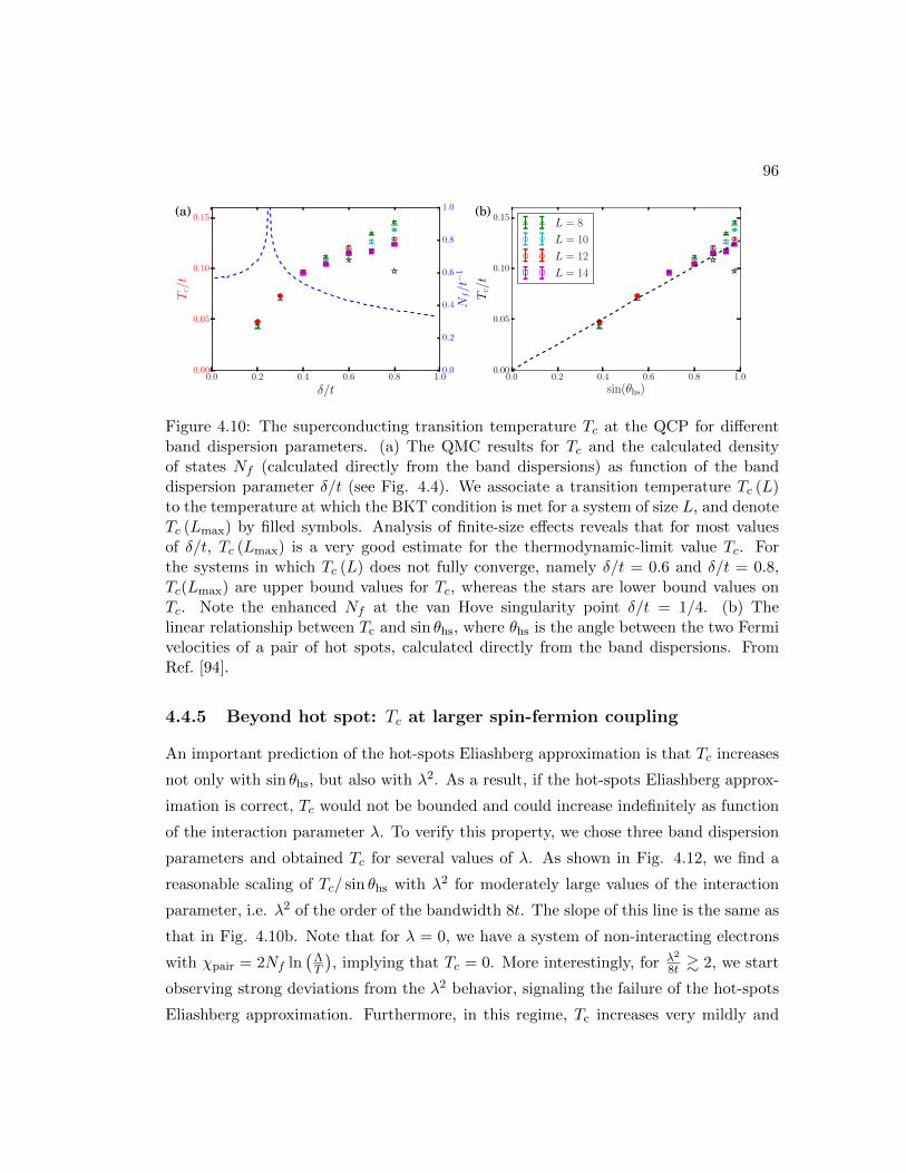
96

0.0 0.2 0.4 0.6 0.8 1.0

δ/t

0.00

0.05

0.10

0.15

Tc/t

(a)

0.0

0.2

0.4

0.6

0.8

1.0

Nf/t−

1

0.0 0.2 0.4 0.6 0.8 1.0

sin(θhs)

0.00

0.05

0.10

0.15

Tc/t

(b)L = 8

L = 10

L = 12

L = 14

Figure 4.10: The superconducting transition temperature Tc at the QCP for differentband dispersion parameters. (a) The QMC results for Tc and the calculated densityof states Nf (calculated directly from the band dispersions) as function of the banddispersion parameter δ/t (see Fig. 4.4). We associate a transition temperature Tc (L)to the temperature at which the BKT condition is met for a system of size L, and denoteTc (Lmax) by filled symbols. Analysis of finite-size effects reveals that for most valuesof δ/t, Tc (Lmax) is a very good estimate for the thermodynamic-limit value Tc. Forthe systems in which Tc (L) does not fully converge, namely δ/t = 0.6 and δ/t = 0.8,Tc(Lmax) are upper bound values for Tc, whereas the stars are lower bound values onTc. Note the enhanced Nf at the van Hove singularity point δ/t = 1/4. (b) Thelinear relationship between Tc and sin θhs, where θhs is the angle between the two Fermivelocities of a pair of hot spots, calculated directly from the band dispersions. FromRef. [94].

4.4.5 Beyond hot spot: Tc at larger spin-fermion coupling

An important prediction of the hot-spots Eliashberg approximation is that Tc increases

not only with sin θhs, but also with λ2. As a result, if the hot-spots Eliashberg approx-

imation is correct, Tc would not be bounded and could increase indefinitely as function

of the interaction parameter λ. To verify this property, we chose three band dispersion

parameters and obtained Tc for several values of λ. As shown in Fig. 4.12, we find a

reasonable scaling of Tc/ sin θhs with λ2 for moderately large values of the interaction

parameter, i.e. λ2 of the order of the bandwidth 8t. The slope of this line is the same as

that in Fig. 4.10b. Note that for λ = 0, we have a system of non-interacting electrons

with χpair = 2Nf ln(

ΛT

), implying that Tc = 0. More interestingly, for λ2

8t & 2, we start

observing strong deviations from the λ2 behavior, signaling the failure of the hot-spots

Eliashberg approximation. Furthermore, in this regime, Tc increases very mildly and

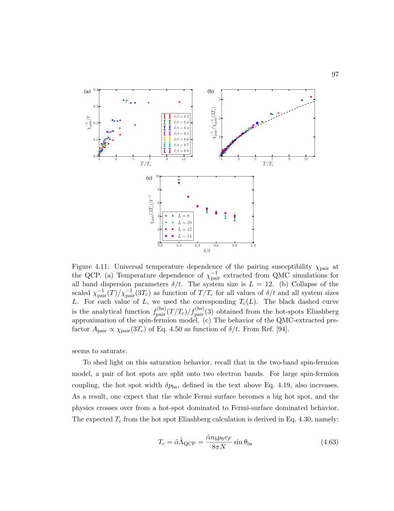
97

1 3 5 7 9 11

T/Tc

0.0

0.1

0.2

0.3

0.4χ−

1p

air/t

(a)

δ/t = 0.2

δ/t = 0.3

δ/t = 0.4

δ/t = 0.5

δ/t = 0.6

δ/t = 0.7

δ/t = 0.8

1 3 5 7 9 11

T/Tc

0

1

2

3

χ−

1p

air/χ−

1p

air(

3Tc)

(b)

0.0 0.2 0.4 0.6 0.8 1.0

δ/t

0

2

4

6

8

10

χp

air(

3Tc)/t−

1

(c)

L = 8

L = 10

L = 12

L = 14

Figure 4.11: Universal temperature dependence of the pairing susceptibility χpair atthe QCP. (a) Temperature dependence of χ−1

pair extracted from QMC simulations forall band dispersion parameters δ/t. The system size is L = 12. (b) Collapse of thescaled χ−1

pair(T )/χ−1pair(3Tc) as function of T/Tc for all values of δ/t and all system sizes

L. For each value of L, we used the corresponding Tc(L). The black dashed curve

is the analytical function f(hs)pair (T/Tc)/f

(hs)pair (3) obtained from the hot-spots Eliashberg

approximation of the spin-fermion model. (c) The behavior of the QMC-extracted pre-factor Apair ∝ χpair(3Tc) of Eq. 4.50 as function of δ/t. From Ref. [94].

seems to saturate.

To shed light on this saturation behavior, recall that in the two-band spin-fermion

model, a pair of hot spots are split onto two electron bands. For large spin-fermion

coupling, the hot spot width δphs, defined in the text above Eq. 4.19, also increases.

As a result, one expect that the whole Fermi surface becomes a big hot spot, and the

physics crosses over from a hot-spot dominated to Fermi-surface dominated behavior.

The expected Tc from the hot spot Eliashberg calculation is derived in Eq. 4.30, namely:

Tc = αΛQCP =αnbp0vF

8πNsin θhs (4.63)

98

0 1 2 3 4 5

λ2/8t

0.0

0.1

0.2

0.3

Tc/t

sin

(θh

s)

δ/t = 0.4

δ/t = 0.6

δ/t = 0.8

Figure 4.12: Dependence of the superconducting transition temperature on the interac-tion strength. For three values of the band dispersion parameter δ/t, we show the QMCresults for Tc, in units of the hopping parameter t and normalized by the correspondingvalue of sin θhs, as function of the squared coupling constant λ2 (in units of 8t) describ-ing how strong the electrons interact with AFM fluctuations. The system size is L = 12.The dashed line, which denotes a λ2 dependence, has the same slope as in Fig. 4.10b,and is expected from the analytical hot-spots Eliashberg solution of the spin-fermionmodel. The absence of the data point corresponding to δ/t = 0.8 and λ2 = 4.5t isbecause Tc did not converge as function of the system size for these parameters. FromRef. [94].

It is clear that Tc becomes independent on the spin-fermion interaction strength as it

becomes larger, consistent with the our QMC results.

4.4.6 Analysis and conclusion

In summary, we showed that within the spin-fermion model the SC properties near

an AFM quantum critical point, including both the transition temperature Tc and the

temperature-dependent pairing susceptibility χpair, are dominated by the properties of

the hot spots, while being rather insensitive to the global properties of the Fermi surface.

More specifically, the functional dependences of Tc and χpair inferred from our QMC

results, given by Eqs. 4.49 and 4.50, are very well captured by an approximate analytical

solution of the spin-fermion model that focuses on the impact of the Landau damping on

the pairing interaction. In other words, the hot-spots Eliashberg approach provides an

99

excellent approximate solution to the spin-fermion model, which presumably should hold

also for systems with different types of band dispersions beyond the rather artifical two-

band case. It is surprising that such an approximation works well even for moderately

large values of the interaction λ2 between the AFM fluctuations and the low-energy

electronic states. However, our combined QMC-analytical analysis also reveals that

when λ2 becomes larger than the electronic bandwidth, the hot-spots approximation

fails. Interestingly, at this crossover from hot-spots dominated pairing to Fermi-surface

dominated pairing, Tc seems to start saturating, signaling that the maximum possible

Tc value for this model has been achieved.

Our results have important implications to the understanding of quantum critical

pairing in general. On the one hand, by establishing that the properties of the hot spots

govern the SC properties of the low-energy spin-fermion model, it offers important in-

sights into which of the many system parameters should be changed to optimize Tc in

an ideal system. For instance, it becomes clear that systems with nearly-nested Fermi

surfaces, where sin θhs is small, despite having an abundance of low-energy magnetic

fluctuations, have a much smaller transition temperature than systems with non-nested

Fermi surfaces, where sin θhs is larger. Conversely, our results establish robust and

well-defined benchmarks that allow one to assess whether the SC state obtained in

other microscopic models or even the superconducting state observed in actual materi-

als falls within the “universality class” of the low-energy spin-fermion model. Two such

benchmarks, for instance, are the linear dependence of Tc on sin θhs and the saturation

of Tc for large interactions. Large-cluster DMFT simulations of the Hubbard model

[113, 114, 115] may be able to test these benchmarks and elucidate whether the super-

conducting properties of the Hubbard model are determined by hot-spots properties or

whether they depend on physics beyond the spin-fermion model. On the experimental

front, the most promising material candidates that show signatures of AFM quantum

criticality near optimal doping are electron-doped cuprates and isovalent-doped pnic-

tides. As for hole-doped cuprates, although they do have a putative AFM quantum

critical point, they also display phenomena that have yet to be observed in QMC sim-

ulations of the spin-fermion model, such as additional intertwined ordered phases [116]

and a transition from small to large Fermi surface without an obvious accompanying

order [117]. One interesting possibility is to investigate how pressure affects Tc in these

100

compounds, and correlate these changes with the pressure-induced modifications of the

hot-spots properties.

4.5 Interplay between superconductivity and charge den-

sity wave physics near an antiferromagnetic quantum

phase transition

4.5.1 Introduction

Charge density wave (CDW) is an electronic order where the electron density exhibits

periodic modulation in real space, namely ρ(r) = ρ0 + ∆CDW exp(iQCDW · r) + h.c..

Here ρ0 is the uniform electron density, and ∆CDW is the CDW order parameter, with

wavevector QCDW. CDW has long been observed and studied. For example, one-

dimensional metals with one electron per unit cell are unstable towards the formation

of a CDW ground state. This is known as the Peierl’s transition[118].

In recent years, short-range CDW order has been detected inside the pseudogap re-

gion in various cuprate materials, such as Ba2Sr2CaCu2O8+x[11, 102], YBa2Cu3O6+x[12],

and HgBa2CuO4+x [103]. The occurrence of CDW is close to the superconducting phase,

and both occur when long-range antiferromagnetic order is suppressed.

The CDW wavevector is along either of the Cu-Cu directions in the CuO2 plane, i.e.,

it is axial. This is shown by scanning tunneling microscopy studies on Ba2Sr2CaCu2O8+x,

as well as resonant X-ray scattering studies on YBa2Cu3O6+x and HgBa2CuO4+x. In

HgBa2CuO4+x, quantum oscillations suggest that the CDW phase is a double-Q state,

where axial CDW with wavevector along both of the Cu-Cu directions coexist micro-

scopically.

The CDW order seems to be a low-energy electronic instability. This is hinted from

the fact that the wavevector is incommensurate with the underlying lattice, and seem-

ingly follows the wavevector connecting the nesting portions of the Fermi surface[103].

If the CDW order is indeed a low energy phenomenon, similar to superconductivity,

then the onset of one order is expected to suppress the other, since both compete for the

same low-energy electrons. This view seems to be consistent with results from X-ray

experiments in hole-doped YBa2Cu3O6+x, that the charge fluctuations are suppressed at

101

the onset of superconductivity, and that by suppressing superconductivity with magnetic

field, charge fluctuations are enhanced. On the other hand, the results on electron-doped

Nd1−xCexCuO4 [119] are a bit confusing, with enhanced charge susceptibility at very

high temperatures, and seemingly uncorrelated with superconductivity.

It remains an open question as to the origin of the charge density wave order. One

view, as presented in earlier sections of this chapter, is that both CDW and supercon-

ductivity are emergent due to spin fluctuations [101, 14]. In particular, in the hot-spot

approximation to the spin-fermion model, there is an emergent particle-hole symmetry

at each hot spot, which maps a Cooper pairing operator onto a charge density wave op-

erator. However, such a CDW operator has a wavevector along the diagonal direction

(called checkerboard CDW) rather than the bond directions of Cu-O-Cu, inconsistent

with the experimental observations of singe-Q/double-Q axial states described above.

Ref. [101] took one step further to show that non-hot-spot properties, in particular, the

nesting properties near the anti-nodal regions on the Fermi surface3 will favor the

axial orders, which can emerge if the spin fluctuations become strong enough (i.e., near

magnetic quantum critical point).

CDW physics in proximity to an antiferromagnetic QCP has been studied in two sep-

arate papers [92, 110] using the Monte Carlo technique described previously. While the

presence of a magnetic QCP does enhance both axial and checkerboard charge fluctua-

tions, the enhancement is found to less than 5% at all temperatures, despite a significant

boost of superconductivity. These results are in contradiction to the theoretical work

presented in Ref. [14], which predicted a near-degeneracy between checkerboard CDW

and superconductivity based on the hot spot approximation.

One possible reason for such a discrepancy is that CDW is a delicate phase that

depends on the fine tuning of the electronic band structure beyond the hot spots. In

particular, the nesting features of the Fermi surface may be crucial to observing any sort

of enhanced CDW correlations. In this section, I present a detailed numerical study of

the two-band spin-fermion model, focusing on purely one-dimensional band dispersions.

Unlike two-dimensional band dispersions, the non-interacting charge susceptibility is

logarithmically divergent at low temperatures, and any small attractions in the charge

sector can induce long-range CDW order.

3 See Fig. 4.1. Antinodal regions correspond to (π, 0) and (0, π) in the Brillouin zone.

102

This section is organized as follows: I will first describe the choice of purely one-

dimensional dispersions, and point out an exact particle-hole symmetry of the spin-

fermion model at half-filling. I will show that in this case, both CDW and supercon-

ductivity are equally enhanced by spin fluctuations, and present the numerical results

to support it. By going away from half-filling, the exact particle-hole symmetry is bro-

ken. However, there is still the approximate particle-hole symmetry coming from the

linearized hot spot approximation. I will show that this approximate symmetry in the

electronic properties is insufficient in supporting a nearly-degenerate superconducting

and CDW order.

4.5.2 One-dimensional band dispersion

We study a series of one-dimensional electronic band dispersions described by the fol-

lowing:

εck = −µ− 2t cos kx

εdk = −µ− 2t cos ky(4.64)

The two electron bands are related by a 90-degree rotation. By tuning the ratio of µ/t,

the wavevector Q0 connecting parallel lines of the Fermi surface change as:

Q0 = 2 arccos−µ2t

(4.65)

In particular, at half-filling µ = 0, the charge density wave wavevector is Q0 = π.

Fig. 4.13 shows the two electronic Fermi surfaces for µ/t = −√

2. Hot spots on each

Fermi surface are marked by purple dots. The momentum dependence and the log-

arithmic behavior of the non-interacting static charge susceptibility are presented in

Fig. 4.14.

4.5.3 Half filling and exact SU(2) symmetry

At half-filling µ = 0, the two-band spin-fermion model has an exact SU(2) symmetry

associated with a bipartite particle-hole transformation P, defined as:

Pψa(r) ≡ iσ2(−1)ix+iyψ∗a(r); ψa ≡ (a↑, a↓)T (4.66)

103

-π π-π

π-π π

-π

π

Figure 4.13: Purely one dimensional Fermi surface used in our studies. Here µ/t = −√

2.Purple points mark the location of the hot spots. Gray dashed line marks the antiferro-magnetic Brillouin zone boundary, and the gray dashed arrow is the antiferromagneticordering wavevector Q = (π, π). The orange arrow Q0 = π/2 connects parallel lines ofthe Fermi surface. This is the CDW wavevector favored by the Fermi surface.

where a = c, d labels the two electron bands. r ≡ (ix, iy) is the lattice coordinate of the

fermion field. ψ∗a ≡ (a†↑, a†↓)T , i.e., without transposing the column vector.

To see this, let’s first write down the full fermion Hamiltonian on a 2D square lattice:

H = −t∑

r

(c†rαcr+xα + d†rαdr+yα

)+ λ

∑

r

~φr · (c†rα~σαβdrβ + h.c.)

= −t∑

r

(ψ†crσ0ψcr+x + ψ†drσ0ψdr+y

)+ λ

∑

r

~φr · (ψ†cr~σψdr + h.c.)

≡ T + V

(4.67)

In the absence of the spin-fermion coupling, the nearest-neighbor hopping gives the

energy dispersion described in Eq. 4.64. The second line is the matrix form in spin

space, with (σ0, ~σ) the Pauli matrices. T and V are short-hand notations for the kinetic

term and the interaction term respectively.

Under the bipartite particle-hole transformation P, the kinetic term (T ) becomes:

TP−→ −t(−1)

∑

r

∑

i=c,d

(iσ2ψ∗i )†σ0(iσ2ψ

∗i )

= −t(−1)∑

r

∑

i=c,d

ψTi (−iσ2)σ0(iσ2)ψ∗i = T(4.68)

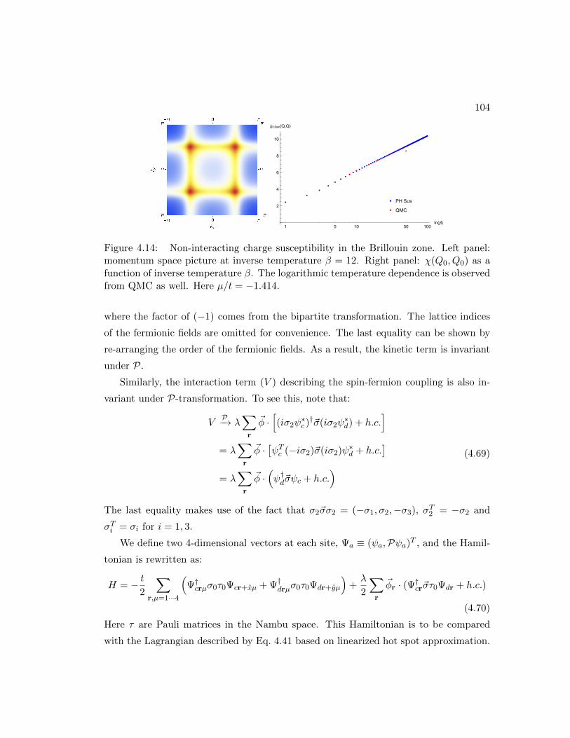
104

PH Sus

QMC

1 5 10 50 100ln(β)

2

4

6

8

10

χCDW(Q,Q)

Figure 4.14: Non-interacting charge susceptibility in the Brillouin zone. Left panel:momentum space picture at inverse temperature β = 12. Right panel: χ(Q0, Q0) as afunction of inverse temperature β. The logarithmic temperature dependence is observedfrom QMC as well. Here µ/t = −1.414.

where the factor of (−1) comes from the bipartite transformation. The lattice indices

of the fermionic fields are omitted for convenience. The last equality can be shown by

re-arranging the order of the fermionic fields. As a result, the kinetic term is invariant

under P.

Similarly, the interaction term (V ) describing the spin-fermion coupling is also in-

variant under P-transformation. To see this, note that:

VP−→ λ

∑

r

~φ ·[(iσ2ψ

∗c )†~σ(iσ2ψ

∗d) + h.c.

]

= λ∑

r

~φ ·[ψTc (−iσ2)~σ(iσ2)ψ∗d + h.c.

]

= λ∑

r

~φ ·(ψ†d~σψc + h.c.

)(4.69)

The last equality makes use of the fact that σ2~σσ2 = (−σ1, σ2,−σ3), σT2 = −σ2 and

σTi = σi for i = 1, 3.

We define two 4-dimensional vectors at each site, Ψa ≡ (ψa,Pψa)T , and the Hamil-

tonian is rewritten as:

H = − t2

∑

r,µ=1···4

(Ψ†crµσ0τ0Ψcr+xµ + Ψ†drµσ0τ0Ψdr+yµ

)+λ

2

∑

r

~φr · (Ψ†cr~στ0Ψdr + h.c.)

(4.70)

Here τ are Pauli matrices in the Nambu space. This Hamiltonian is to be compared

with the Lagrangian described by Eq. 4.41 based on linearized hot spot approximation.

105

The Hamiltonian is invariant under the SU(2) transformations in the Nambu space (τ),

as the only matrix appearing in the Hamiltonian is the identity matrix τ0. Below I

show the implications of such a symmetry to superconductivity and CDW. Unlike the

hot spot SU(2) discussed previously in Sec. 4.2, where the Cooper pairing and CDW

operators are mapped onto each other, here the bipartite SU(2) does not lead to such

a mapping. As I show below, the susceptibilities do map onto each other in the high-T

disordered phase.

Note that the sign-changing superconducting and CDW vertices are:

ΓSC(r, τ) = ∆iσ2αβ (cαcβ − dαdβ) (4.71)

ΓCDW(r, τ) = ρσ0αβ

(c†αcβ − d†αdβ

)(4.72)

where ∆ and ρ are the superconducting and CDW order parameters respectively. The

corresponding susceptibilities:

χi(r, τ) = 〈Γi(r, τ)Γ†i (0, 0)〉 (4.73)

Here we show how the s± superconducting and (π, π) CDW are degenerate due to this

symmetry. Starting from the pairing susceptibility, we have:

χSC = (iσ2,αβ)(−iσ∗2,γδ)〈(crαcrβ − drαdrβ)(c†0δc

†0γ − d†0δd

†0γ

)〉 (4.74)

where for simplicity we neglected the imaginary time indices. There are four terms after

expanding out the parenthesis, all in the form of:

χijSC = (iσ2,αβ)(iσ2,γδ)〈ψi,rαψi,rβψ†j,0δψ†j,0γ〉

= (iσ2,αβ)(iσ2,γδ) (−〈13〉〈24〉+ 〈14〉〈23〉)= −2(iσ2,αβ)(iσ2,γδ)〈13〉〈24〉

(4.75)

where i, j = c, d, and 1 · · · 4 label the fermionic creation/annihilation operators by their

respective positions in the expression. The last equality can be shown straightforwardly.

Now I show that this can be transformed into the CDW susceptibility. To see this, note

that under P transformation:

χijSC = −2(iσ2,αβ)(iσ2,γδ)〈ψi,rαψ†j,0δ〉〈ψi,rβψ†j,0γ〉

= −2(−1)ix+iy(iσ2,αβ)(iσ2,γδ)(iσ2αm)(iσ2δn)〈ψ†i,rmψj,0n〉〈ψi,rβψ†j,0γ〉

= 2(−1)ix+iy (σ2mασ2,αβσ2,γδσ2δn) 〈ψ†i,rmψj,0n〉〈ψi,rβψ†j,0γ〉

= 2(−1)ix+iyσ0,mβσ0,nγ〈ψ†i,rmψj,0n〉〈ψi,rβψ†j,0γ〉

(4.76)

106

This is equal to twice the corresponding term in the CDW susceptibility:

χijCDW ≡ σ0,αβσ0,δγ〈ψ†i,rαψi,rβψ†j,0γψj,0δ〉

= σ0,αβσ0,δγ〈ψ†i,rαψj,0δ〉〈ψi,rβψ†j,0γ〉

(4.77)

The sign factor of (−1)ix+iy means superconducting susceptibility at q = 0 is equal to

CDW susceptibility at q = (π, π). Unlike the approximate SU(2) symmetry from hot

spot approximation, here the symmetry is exact due to half filling. Away from half

filling, µ 6= 0, the bipartite particle-hole symmetry is broken.

4.5.4 Main results from DQMC

We studied a series of purely one-dimensional band dispersions using DQMC, using µ/t

as a tuning parameter. We studied system sizes L = 8, 10, 12. Unless finite size effects

are significant, I will focus on the results obtained for only L = 12. Additionally, we

choose t = 1, and measure all other energies in units of t.

Below we will only look at charge and superconducting instabilities where there is

a sign-change between the two electron bands.

Half-filling

Fig. 4.15 shows the static charge and superconducting susceptibilities at a fixed tem-

perature β = 12 at the magnetic QCP. The maximum of the charge susceptibility is

at (π, π), as expected. There is no apparent enhancement for the stripe CDW with

wavevectors (π, 0) or (0, π). The maximum of SC susceptibility is at (0, 0), suggesting

the absence of pair density wave order.

Fig. 4.16 shows the charge and pair susceptibilities divided over the non-interacting

value for various temperatures and distance to magnetic QCP. Both susceptibilities are

enhanced in proximity to the magnetic QCP. More interestingly, the two susceptibilities

lie within errorbars of each other at the same temperatures, suggesting that the particle-

hole symmetry described above is observed from numerics.

Next we look at the superconducting transition temperature. Theoretically, since

there is an exact SU(2) symmetry, in two dimensions there is no long range order with a

finite transition temperature. Nonetheless, the correlation length grows as temperature

goes down, suggesting a zero-T symmetry breaking. Numerically, only finite system sizes

107

-π π-π

π-π π

-π

π

-π π-π

π-π π

-π

π

Figure 4.15: Charge (left) and superconducting (right) susceptibilities in the momen-tum space at the magnetic QCP. Half-filling at µ = 0, β = 12. The maximum of theCDW susceptibility is at (π, π), consistent with expectations. The maximum of SCsusceptibility is at (0, 0), suggesting the absence of pair density wave order.

can be simulated. When the correlation length grows bigger than the linear dimension, it

will resemble a transition into an ordered phase, as averaging over the space-time gives a

finite order parameter. However, the transition temperature should exhibit strong finite

size effects, and extrapolate to zero in the thermodynamic limit. In Fig. 4.17 I show

the behavior of superfluid density ρs as well as the superconducting Tc defined by the

Berezinskii-Kosterlitz-Thouless criterion. Both the superfluid density and the transition

temperature Tc(L) exhibit strong finite size effects for the three system sizes L = 8, 10, 12

we have studied. Although inconclusive, the strong size dependence suggests the absence

of true long range order at finite temperatures.4

Away from half-filling

Away from half-filling, the particle-hole symmetry is absent. Nonetheless, CDW can still

emerge due to spin fluctuations[101]. We studied four different band dispersions, with

Q0 = πi/6, where i = 2, 3, 4, 5, corresponding to period-6, period-4, period-3 and period-125 charge density wave orders. These are achieved by µ/t = −

√3,−√

2,−1,−12 arccos 5

12

4 The computation time scales exponentially with the lattice dimension L, due to calculation ofthe fermion determinant, see appendix A. Therefore, L = 12 is the maximum system size we haveinvestigated.

108

β=

β=

β=

χ/χ

χ/χ

Figure 4.16: d-wave charge (left) and superconducting (right) susceptibilities plottedversus distance to magnetic QCP for temperatures β = 6, 10, 16.

respectively. The choice of the periods are because these are the exact wavevectors that

can be probed in DQMC for L = 12.

Fig. 4.18 shows the static charge susceptibility in momentum space at the magnetic

QCP. All results are presented for β = 12. The location of the maximum charge

susceptibility is consistent with the wavevectors favored by the respective Fermi surfaces.

In Fig. 4.19, we show the dependence of the superconducting and CDW suscepti-

bilities on the distance to magnetic QCP for the four band dispersions. Although both

SC and CDW are enhanced by the presence of quantum critical spin fluctuations, SC is

enhanced much stronger compared to CDW. The lifting of the CDW-SC degeneracy is

already quite apparent at Q0 = 5π/6, i.e. a small deviation from half-filling, suggesting

the extreme sensitivity of charge order to the exact particle-hole symmetry.

To illustrate the competition between CDW and superconductivity, in Fig. 4.20 we

plot the temperature evolution of superconducting and charge susceptibilities at the

magnetic QCP for the electronic band dispersion corresponding to period-4 CDW. At

high temperatures, both susceptibilities increase as temperature goes down, suggesting

the tendency towards long range order. However, near the onset of the superconducting

phase via a BKT transition, the charge susceptibility decreases with decreasing tem-

perature, suggesting that the presence of long-range superconducting order suppresses

109

=

=

=

ρ

/

Figure 4.17: Left: superfluid density versus temperature for L = 8, 10, 12. Right:extracted BKT transition temperature Tc(L). Finite size effects are significant in theseproperties.

-π π-π

π-π π

-π

π

-π π-π

π-π π

-π

π

-π π-π

π-π π

-π

π

-π π-π

π-π π

-π

π

Figure 4.18: Charge susceptibilities in the momentum space for period-125 , period-3,

period-4 and period-6 charge density wave orders. All results are obtained at the mag-netic QCP. β = 12.

CDW. This is consistent with X-ray measurements on YBa2Cu3O6+x [12], as well as

other theoretical calculations [120].

Can stripe CDW fluctuations be favored over the checkerboard CDW fluc-

tuations?

As has been discussed above, at the magnetic QCP, the maximum charge susceptibility

is always located along the diagonal direction. While this is expected based on the hot

spot approximation to the spin-fermion model, it is not consistent with experimental

results.

In Fig. 4.21 we show the comparison of the charge susceptibility in the magnetically

ordered phase and at the magnetic QCP. The results are obtained for the electronic

band dispersion favoring a period-4 CDW. It is obvious that in the magnetically ordered

110

χ/χ

χ/χ

χ/χ

χ/χ

χ/χ

Figure 4.19: Charge and superconducting susceptibilities for a inverse fixed tempera-ture β = 12. The band dispersions correspond to half-filling (top), period-12

5 (middleleft), period-3 (middle right), period-4 (bottom left) and period-6 (bottom right) CDW.

phase, the maximum of the charge susceptibility is along the Cu-O-Cu bond directions.

In the right panel of Fig. 4.21, we quantify the checkerboard to axial CDW evolution

by defining the ratio of the maximum charge susceptibility along diagonal and bond

directions: χ(Q0, Q0)/χ(Q, 0).5 This ratio has a sharp change at the magnetic QCP,

suggesting that axial CDW correlations are favored when the Fermi surface undergoes

a reconstruction due to the onset of long range magnetic order. A qualitative argument

has been given based on nodal/antinodal asymmetry of the Fermi surface due to the

5 Due to Fermi surface reconstruction in SDW phase, the maximum charge susceptibility may notsit exactly at Q0.

111

χ-

TBKT

Figure 4.20: Inverse charge and superconducting susceptibilities versus temperature atthe magnetic QCP.

-π π-π

π-π π

-π

π

-π π-π

π-π π

-π

π

χ ( )

χ ( )

Figure 4.21: Charge susceptibilities in the magnetically ordered phase (left) versusat the magnetic quantum critical point (middle). Results obtained based on the banddispersion favoring period-4 CDW. The ratio between the maximum charge susceptibil-ities along the Cu-O-Cu bond direction and the diagonal direction is shown in the rightfigure. The arrow marks the location of the magnetic QCP.

opening of an enegy gap at the hot spots [101].

4.5.5 Analysis and conclusion

By considering purely one dimensional band dispersions, we find signatures of charge

density wave order numerically within the two-band spin-fermion model. Through

Fig. 4.16 and 4.19, we see that charge susceptibility is enhanced in proximity to an

antiferromagnetic QCP, suggesting the possibility of CDW induced by quantum spin

fluctuations.

By contrasting the results for band dispersions at and away from half-filling, we

112

see that the CDW is very delicate, requiring Fermi surface fine tuning, and loses to

superconductivity very quickly when the exact particle-hole symmetry is broken. The

competition between SC and CDW is evident from the numerical results, in particular,

from Fig. 4.20. The degeneracy lifting is already apparent at temperatures above the

superconducting phase. One method to understand it is through the negative feedback

of superconducting fluctuations on charge density wave fluctuations.

We also analyzed the checkerboard versus axial CDW correlations. As is shown in

Fig. 4.21, the axial CDW correlations can only be favored in the magnetically ordered

phase, when the Fermi surface develops an energy gap at the hot spots.

4.6 Conclusions

In this chapter, we discussed several aspects of the low-energy electronic phase diagram

of cuprate high temperature superconductors, focusing on the proximity to an antifer-

romagnetic quantum critical point. We investigated the so-called spin-fermion model,

which is a low-energy effective model describing quantum critical spin fluctuations cou-

pled to electrons near the Fermi surface. By combined analytical and numerical work, we

revealed the low energy physics of the model, and how microscopic system parameters

govern the superconducting and charge density wave properties.

In Sec. 4.2, following past works [13, 14, 101], we presented an analytical solution of

the spin-fermion model. In particular, based on the Eliashberg approach, we discussed

the importance of special points on the Fermi surface called hot spots, and how their

properties uniquely determine the superconducting properties. We also pointed out

a special particle-hole symmetry due to the linearized hot spot approximation, which

gives rise to an emergent symmetry between superconductivity and charge density wave.

This gives a qualitative argument why in many cuprate materials, superconductivity and

charge density wave order are found near each other in the phase diagram.

In Sec. 4.4, we presented a numerical solution of the spin-fermion model using a

Determinantal Quantum Monte Carlo technique, focusing on the superconducting prop-

erties in proximity to an antiferromagnetic quantum critical point. By carefully tuning

the low-energy electronic properties, in particular those relevant to the hot spots, we

113

discovered a functional dependence of superconducting transition temperature and sus-

ceptibility on the hot spot properties (Eq. 4.49 and 4.50). We find a remarkable agree-

ment between the numerical solutions and those predicted by the hot spot Eliashberg

approach. We also studied the failure of the hot spot approximation by going to large

spin-fermion interactions, and concluded that the saturation of Tc is due to the whole

Fermi surface acting like one big hot spot.

In Sec. 4.5, we studied the possibility of a charge density wave order in the spin-

fermion model, and discussed its interplay with superconductivity. We studied a series

of purely one-dimensional electronic band dispersions at and away from half-filling. We

find that the while both superconductivity and charge density wave order are enhanced

due to the presence of quantum critical spin fluctuations, charge density wave is a rather

delicate order extremely sensitive to the fine-tuning of the electronic band dispersion

beyond the hot spot properties. In particular, charge density wave is quickly suppressed

away from half-filling, where an exact particle-hole symmetry guarantees the degeneracy

between charge density wave and superconductivity.

Chapter 5

Conclusion

In this thesis, I discussed several aspects of the phase diagram of high-Tc cuprate and

iron pnictide/chalcogenide superconductors, and addressed several important questions

pertaining to the research community.

In Ch. 2, I investigated the nature and origin of the magnetic phases in the iron

pnictide materials. Comparing the magnetic phase diagrams arising from a localized

J1-J2 spin-Heisenberg model, and from an itinerant model describing weakly interacting

electrons near the Fermi surface, I showed that the magnetic orders which preserve

square lattice symmetry naturally occurs only in the itinerant model. I showed how these

magnetic orders can become the ground state due to imperfect Fermi surface nesting

(induced by doping, pressure etc.), the residual electronic interactions (i.e., interactions

which do not contribute directly to the magnetic instabilities), and the effect of Neel

antiferromagnetic fluctuations (induced by doping local magnetic moments). Since the

existence of tetragonal magnetic orders is crucial in identifying the microscopic origin

of magnetism, I proposed unique experimental manifestations of these orders in the

electronic properties and collective spin excitations.

In Ch. 3, I investigated the origin of electronic nematic order in the iron pnictide

materials. In particular, I discussed in detail the magnetic scenario, where nematic

order is driven by strong magnetic fluctuations. I showed that while at a mean-field

level, the nematic order and the magnetic order occur simultaneously, once fluctua-

tions are accounted for, the two transitions can be split. I proceeded to discuss the

114

115

experimental manifestations of electronic nematicity, focusing on its effect on the lo-

cal density of states near an impurity, which can be visualized by atomically-resolved

spectroscopy. Through the successful modeling of the results obtained by scanning tun-

neling spectroscopy, I demonstrated the intimate relationship between nematicity and

large amplitude magnetic fluctuations in iron pnictide materials.

In Ch. 4, I investigated the physics of superconductivity (SC) and charge density

wave (CDW) near a metallic antiferromagnetic quantum critical point (QCP). By nu-

merically solving the spin-fermion model via a sign-problem-free Quantum Monte Carlo

technique, I showed the significance of hot spot properties in uniquely determining

the superconducting transition temperature and the superconducting fluctuations in

proximity to the antiferromagnetic QCP. The numerical results on SC have remarkable

quantitative agreement with those calculated by an approximate field-theoretic method,

reminiscent of the Eliashberg approach used in the electron-phonon problem. This result

is somewhat surprising, and requires further investigations. I also discussed the CDW

physics in the spin-fermion model, and studied its interplay with SC. The numerical

results reveal the competition between SC and CDW, consistent with other theoretical

calculations and experimental results. By studying a series of electronic band disper-

sions, I showed that the CDW is a delicate phase, sensitive to the fine tuning of the

band properties beyond the hot spots.

Appendix A

Determinantal Quantum Monte

Carlo and Application to two

band spin-fermion model

A.1 Monte Carlo basics

Statistical systems are composed of macroscopic number of particles. At thermal equi-

librium they are characterized by their phase space Ω and probability distribution ρ,

with the condition∫

Ω ρ = 1. ln ρ is an additive quantity of the system, and therefore can

be represented by integrals of motion, i.e., ln ρ = −βE+(...), where E is the total energy

of the system, β the inverse temperature. (...) are other integrals of motion (linear and

angular momentum, particle number etc.). Thermodynamic observables are averaged

quantities 〈O〉 ≡∫

ΩOρ. For example, the phase space of a classical N -particle system

is the set of position and momentum of each individual particle: dΩ = ΠNi=1dqidpi, and

ρ ∝ exp(−βE) the probability density. For quantum systems, the phase space consists

of many-body quantum states Σi, and ρ ∝ 〈Σi| exp(−βH)|Σi〉. For quantum field

theories, the phase space consists of paths in field configurations φ(r, τ), and the

probability ρ ∝ exp(−Sφ(r, τ)), where S =∫r,τ L is the action.

With the knowledge of Ω, ρ, we can compute all thermodynamic properties of the

system. In reality, due to the interactions between constituents, seldomly do we have

116

117

analytical solutions. On the other hand, it is precisely the interactions that drive various

phases of matter, such as superconductivity and magnetism.

Monte Carlo (MC) is a powerful numerical method for understanding the properties

of interacting systems. The basic idea is to generate a finite ensemble M of configura-

tions Ω, where the probability of finding a certain configuration Σi ∈ Ω is

P (Σi) =ρ(Σj)∑Mj=1 ρ(Σj)

(A.1)

While the physical observable is:

〈O〉Ω ≡1

M

M∑

i=1

O(Σi) (A.2)

In the limit of M → ∞, the expectation value of physical observables converge to the

thermodynamic properties.

The Monte Carlo method is based on the detailed balance principle, which states that

for statistical system at thermal equilibrium, each elementary process is equilibrated

with its reverse process. Take two states of the system i and j. Detailed balance

principle requires that

ρiWi→j = ρjWj→i (A.3)

where ρi is the thermal equilibrium probability density, and Wi→j the transition prob-

ability from i to j.

Based on the detailed balance principle, the MC ensemble can be constructed fol-

lowing a Markov process described as follows:

(1) Start from a initial configuration Σ0, compute the thermal probability density

ρ0 ≡ 〈exp(−βH)〉0. Generate new configurations successively based on the Markov

transition probability Wi→i+1.

(2) For the (i + 1)th iteration, construct a trial configuration Σi+1, and compute

ρi+1. Accept the trial configuration with probability Wi→i+1. If ρi+1 > ρi, Wi→i+1 = 1;

If ρi+1/ρi < 1, Wi→i+1 = ρi+1/ρi.

The definition of the transition probability is consistent with the detailed balance

principle. Therefore, as the number of iterations goes to infinity, the thermodynamic

limit is reached.

118

A.2 Applications to coupled boson-fermion system

This section reproduces the results previously published in Ref. [105].

In the path-integral formulation, the coupled boson-fermion system we are interested

in is described by a space-time local action:

S = Sφ +

∫dτddx ψ(x, τ) (∂τ +H)ψ(x, τ) (A.4)

where τ ∈ (0, β) is the imaginary time going from 0 to inverse temperature β. Sφ denotes

the bosonic action. φ describes a generic boson field, and ψ ψ are anticommuting

Grassmann variables describing fermionic fields. Note that both φ and ψ can have

multiple components. H ≡ T +V is the fermion Hamiltonian density, with T the kinetic

energy and V the boson-fermion interaction. The partition function: Z =∫

Ω exp(−S),

and the phase space Ω consists of bosonic and fermionic paths in space-time.

In doing Monte Carlo study, both imaginary time and space are discretized to form

a d + 1 dimensional lattice. Since the imaginary time axis is finite, it is discretized to

N steps, with ∆τ ≡ β/N . The discretization error is O(∆τ ). The space is discretized

into Ld lattice points, with linear dimension L. Note that the space is truncated to a

volume of Ld with a certain boundary condition. This inevitably introduces finite size

effects, which I will describe later.

Since Grassmann variables are not c-numbers, and cannot be directly sampled, the

logic is to integrate out the fermionic degrees of freedom, which are described by Gaus-

sian fluctuations, to obtain an effective probability density for the boson fields:

ρ ∝ exp(−Seff) ≡ exp(−Sφ) detτ,x∂τ +H (A.5)

where the fermion determinant is formally defined as detx,τ∂τ +H. While the bosonic

action is local in space and time, the fermion determinant is inherently non local. The

size of the matrix is nNLd × nNLd, where n is the local Hilbert space of fermions. As

a result, the computation complexity of the fermion determinant is then O((nNLd)3)

(e.g., using LU factorization). This is a daunting task, and strongly limits the lattice

size that can be studied using Monte Carlo method.

However, it is easy to see that the fermion determinant is sparse along the τ axis,

in that it connects between adjacent time only. The fermionic action can be written

119

explicitly as (neglecting spatial index):

∫dτψ (∂τ +H)ψ ≡

N∑

i=1

ψiψi + ψi (−1 + ∆τHi−1)ψi−1 (A.6)

where ψ ≡ (ψ1 · · ·ψnLd) is a vector in space, and H is a nLd × nLd matrix. Casted in

a matrix form (ψN = −ψ0):

(ψ0 ψ1 · · · ψN−1

)

1 0 · · · 0 (1−∆τHN−1)

−(1−∆τH0) 1 · · · 0 0...

.... . .

......

0 0 · · · 1 0

0 0 · · · −(1−∆τHN−2) 1

ψ0

ψ1

...

ψN−1

(A.7)

As a result, the fermion determinant shown in Eq. A.5 becomes:

detτ,x = detx I +BN−1 · · ·B1B0 (A.8)

where Bi ≡ 1−∆τHi ≈ exp(−∆τHi). The exponential form is used to reduce discretiza-

tion error. The complexity of evaluating the fermion determinant is O(N(nLd)3), much

reduced compared to taking the full determinant.

A.3 Computing fermionic Green’s function

The calculation of one-particle fermionic Green’s function is shown as follows:

G(x, τ ; x′, τ ′) ≡ 〈T[ψ(x, τ)ψ†(x′, τ ′)

]〉

=1

Z

∫exp(−SB) detx,τ∂τ +HG(x, τ ; x′, τ ′)

(A.9)

where

G(x, τ ; x′, τ ′) ≡ 1

detx,τ∂τ +H

∫exp(−SF )T

[ψ(x, τ)ψ†(x′, τ ′)

](A.10)

is the Green’s function for a fixed bosonic configuration. Again, the calculation of G can

be simplified by utilizing the specific time dependence of the fermionic Hamiltonian. By

defining G(x, τ ; x′, τ ′) ≡ 〈x|G(τ, τ ′)|x′〉, we have:

G(τ, τ ′) = U(τ, τ ′)J−1(τ ′) if β > τ > τ ′

= −U(τ, 0)U(β, τ ′)J−1(τ ′) if β > τ ′ > τ(A.11)

120

where U(τ, τ ′) ≡ T exp(−∫ τ ′τ H), and J(τ) ≡ I+U(τ, 0)U(β, τ). We can show that the

above definition satisfies

(∂τ +H)G(τ, τ ′) = δ(τ − τ ′)I (A.12)

for τ 6= τ ′. The τ = τ ′ criterion is satisfied with:

limε→0+

G(τ ′ + ε, τ ′)− G(τ ′ − ε, τ ′) = I (A.13)

In the discretized time scheme, we have for (i+1)∆τ > τ > i∆τ , (j+1)∆τ ′ > τ ′ > j∆τ ′ ,

and i ≥ j:

G(τ, τ ′) = Bi−1Bi−2 · · ·Bj+1Bj (I +Bj−1 · · ·B0BN−1 · · ·Bj)−1 (A.14)

The equal time Green’s function G(τ, τ − 0+), which is particularly useful in devising

the Monte Carlo algorithm, is:

G(τ, τ − 0+) ≡ Gi = (I +Bi−1 · · ·B0BN−1 · · ·Bi)−1 (A.15)

To move forward along the imaginary time axis (i.e., going from the time slot (i+1)∆τ >

τ > i∆τ to (i+ 2)∆τ > τ > (i+ 1)∆τ ):

Gi+1 = BiGiB−1i (A.16)

The occupation number at a given time slice is given by:

ni ≡ 〈ψ†(τ)ψ(τ − 0+)〉 = I − Gi (A.17)

A.4 Monte Carlo procedure

This section reproduces the results previously published in Ref. [91, 92].

From the above analysis, the coupled boson-fermion system is reduced to an ef-

fective bosonic problem, with probability density given by Eq. A.5. The Monte Carlo

procedure for solving the coupled boson-fermion system, which goes under the name of

Determinantal Quantum Monte Carlo (DQMC), is described as follows:

The procedure starts by specifying an initial bosonic configuration on the discretized

space-time lattice, and constructing the initial fermionic equal-time Green’s function at

121

τ = 0. The Markov chain proceeds by proposing a space-time local change to the

bosonic configuration, and computing the change in the fermion determinant as well

as the bosonic action. The criterion for accepting/rejecting the change is based on the

detailed balance principle, and discussed in Sec. A.1. When all the space in a time slice

has been scanned, proceed to the next time slice. One iteration is completed after the

field configuration on the entire lattice has been updated.

The most time consuming procedure per DQMC iteration is computing the change

in the fermion determinant as well as updating the Green’s function once the proposed

change is accepted. Below I show how they are computed.

At a given time slice (m+ 1)∆τ > τ > m∆τ , let us propose a change in the field at

x0. The ratio of the fermion determinant before and after the change is

R =detxI +Bm−1 · · ·B0BN−1 · · ·B′mdetxI +Bm−1 · · ·B0BN−1 · · ·Bm

(A.18)

where Bi ≡ exp(−∆τHm) ≈ exp(−∆τT ) exp(−∆τVm). The change in the field gives

rise to

B′m ≈ exp(−∆τT ) exp(−∆τV′m) = Bm exp(−∆τ (V ′m − Vm)) ≡ Bm(I +N) (A.19)

where N ≡ exp(−∆τ (V ′m − Vm))− I is a matrix which is non-zero only at (x0,x0). As

a result,

R =detxI +Bm−1 · · ·B0BN−1 · · ·Bm(I +N)

detxI +Bm−1 · · ·B0BN−1 · · ·Bm

=detxG−1

m + (G−1m − I)N

detx G−1m

= detxI + (I − Gm)N= detx0I + (I − Gm)N

(A.20)

where detx0 denotes the local fermionic Hilbert space (spin, orbital etc.) at site x0. As

a result, with the knowledge of the equal-time Green’s function Gm, the time cost of

computing the determinant ratio is O(n3), and it does not scale with lattice size.

Once the proposed change in the bosonic field is accepted, the new equal-time

122

Green’s function needs to be calculated. The updated Green’s function is:

G′m =(I +Bm−1 · · ·B0BN−1 · · ·B′m

)−1

=[G−1m + (G−1

m − I)N]−1

= [I + (I − Gm)N ]−1 Gm

(A.21)

The computation of the matrix inverse go as follows. N is a sparse matrix whose only

nonzero entry resides in a n×N block at (x0,x0). Therefore, only n columns of I −Gmmultiplies N . We can define u v as N × n matrices, with u the n columns of I − Gm,

and v the n rows of N . As a result,

G′m =(I + uv†

)−1Gm = Gm − u

(1 + v†u

)−1v†Gm (A.22)

The last step utilizes the Shermann-Morrison formula : (1+uv†)−1 = 1−u(1+v†u)−1v†.

Therefore, the matrix inverse is on a n× n matrix rather than nLd × nLd matrix. The

total computation complexity is O(L2d), rather than O(L3d) if computed directly.

A.5 Fermion sign problem

A basic assumption for applying the DQMC method is to have a positive transition

probability Wi→i+1. From Eq. A.5, the sampling probability density is proportional to

the fermion determinant. The determinant detxI + BN−1 · · ·B0 is not necessarily

positive definite, and can even become complex, due to the time-ordering of the B

matrices. As a result, the transition probability used in the Markov process is ill-

defined. The sign problem is less of an issue at high temperatures, where the variation

of fields is slow in time, and BN−1 · · ·B0 ≈ exp(−βH) is Hermitian. It becomes rather

severe at low temperatures, where the most interesting physics of phases of matter and

phase transitions occur.

Despite no general way around the sign problem, there are certain classes of Hamil-

tonians where such a sign problem is absent. Ref. [107] presents a sufficient criterion for

sign-problem-free DQMC calculations: if the fermionic Hamiltonian is invariant under

an anti-unitary transformation, then the fermion determinant is positive definite. Such

an anti-unitary transformation A satisfies the following conditions:

A2 = −1; AHA−1 = H (A.23)

123

In the presence of such a symmetry, the Hamiltonian possesses a Kramers doublet. As

a result, all eigenvalues have a corresponding complex conjugate pair. Models which fall

in this category include the negative-U Hubbard model, positive-U Hubbard model at

half-filling, etc.. Generic spin-fermion models do not possess such a symmetry. However,

as I will show below, a two-band generalization can be constructed for DQMC studies.

A.6 Sign-problem free DQMC for two-band spin-fermion

model

The spin fermion model describes the coupling between a vector boson ~φ with the spin

of itinerant electrons. The coupling is assumed to be Yukawa-type, i.e.,

V = λ∑

i

~φi · ψ†iα~σαβψiβ (A.24)

where λ is the Yukawa coupling strength, i is the lattice label, and ~σ are Pauli matrices

in spin space. The kinetic energy of the electrons can also be written on a lattice, with

T =∑

ij;α

(−tij − µδij)ψ†iαψiα (A.25)

where tij is the hopping amplitude between site i and j, and µ the chemical potential

(working with canonical ensemble).

The one-band spin-fermion model does not possess such an anti-unitary symmetry

described previously, therefore suffers from sign problem when performing DQMC. How-

ever, the sign problem is absent for a two-band spin-fermion model, where the vector

boson scatters electrons between different flavors:

V ′ = λ∑

i

~φi ·(c†iα~σαβdiβ + h.c.

)(A.26)

where c and d are annihilation operators for two electron flavors. Written in a matrix

form:

V ′ = λ∑

i

~φi ·(c†↑ c†↓ d†↑ d†↓

)(0 ~σ

~σ 0

)

c↑

c↓

d↑

d↓

≡ λ

∑

i

~φi ·Ψ†~σ ⊗ τ1Ψ (A.27)

124

where ~τ are Pauli matrices in the flavor basis, and ⊗ means the direct product of two

matrices. It is easy to verify that A ≡ iσ2 ⊗ τ3C is the anti-unitary symmetry of the

Hamiltonian, where C is the complex conjugation operator. To see this, note that:

A−1(~σ ⊗ τ1)A = −iσ2 ⊗ τ3(~σ∗ ⊗ τ1)iσ2 ⊗ τ3 = −(−iσ2~σ∗iσ2)⊗ (τ3τ1τ3) (A.28)

The last equation is equal to ~σ ⊗ τ1 following the anticommuting algebra of the Pauli

matrices.

A.7 XY spin and simplification of the fermionic Hamilto-

nian

In the DQMC technique, the most time consuming procedure is the computation of the

fermion determinant, defined in Eq. A.8. This strongly limits the system sizes we can

study. In this section, I will show that if the vector boson has two components (i.e.,

XY spin) rather than three (i.e., Heisenberg spin), there is a spectral symmetry that

reduces the local fermionic Hilbert space from 4 (i.e., spin×band) to 2. Note that going

from Heisenberg to XY spins do not alter the low-energy electronic phase diagram at a

qualitative level.

To see this, let us consider ~φ = (φx, φy). As a result, the vector boson flips of the

spin of the electron when it is scattered from one band to to other. We can define two

spinors as:

ψ1 ≡ (c↑, d↓)T ; ψ2 ≡ (c↓, d↑)

T (A.29)

The spin-fermion interaction Hamiltonian Eq. A.27 can be rewritten to be:

V ′ = λ∑

i

(ψ†1i~φ · ~σψ1i + ψ†2i~φ · ~σ∗ψ2i

)(A.30)

It is easy to see that the fermion Hamiltonian can be written as a direct sum of two

2× 2 blocks:

H = H1 ⊕H2 (A.31)

where the H1 = H∗2 . As a result, the fermion determinant defined in Eq. A.8 can be

recast as:

∑

a=1,2

det x

I(a) +B

(a)N−1 · · ·B

(a)0

⇒∣∣∣det x

I(1) +B

(1)N−1 · · ·B

(1)0

∣∣∣2

(A.32)

125

Such a reduction of dimensionality comes from the fact that spin rotation symmetry

for XY spins has a one-dimension faithful representation, in the form of (φx, φy) ⇔|φ| exp(iθ). For Heisenberg spins, such a reduction does not exist.

A.8 Reducing finite size effects using a magnetic flux

One common issue associated with Monte Carlo simulations is finite size effects. In

our DQMC procedure, the system is placed on a L × L square lattice. To extrapolate

to the thermodynamic limit, large system sizes needs to be studied. However, due to

limitations in the computing resources, the maximum linear dimension we can study

is on the order of 10. Finite size effects are severe when extracting various critical

temperatures for the onset of long range order, such as superconductivity and charge

density wave.

There is an even bigger problem associated with simulations on a finite lattice, due to

insufficient sampling of the electronic states. To illustrate this problem, we consider the

example of applying periodic boundary conditions to the fermionic degrees of freedom,

namely:

cr = cr+Lx = cr+Ly = cr+Lx+Ly (A.33)

where x/y are unit vectors along the x y directions. As a result, in the Brillouin zone,

only states with wavevectors k = 2πL (lx, ly); lx/y = 1...L are included in the calculations.

On the other hand, at low temperatures, the physics is determined by electronic

states near the Fermi surface, which is a one-dimensional submanifold of the two-

dimensional Brillouin zone. As a result, out of the L2 momentum states, only O(L)

states are responsible for the physics of various electronic orders. Finite size effects

become extremely severe in computing low-energy electronic properties. In Fig. A.1, I

show how the finite system size affects the compressibility of the non-interacting system.

To reduce the finite size effects, we follow Ref. [108, 92] to thread a magnetic flux

quanta Φz = h/e through the two-dimensional square lattice. Qualitatively, the re-

duction of finite size effects due to a magnetic flux can be understood as follows: The

presence of a boundary has a stronger effect on delocalized electrons (e.g., in a metal)

than localized electrons (e.g., in an insulator). The presence of a magnetic flux can

localize electronic states, therefore reducing the effects caused by having a boundary.

126

Figure A.1: Compressibility of the non-interacting electronic system, calculated fromdensity-density correlation function. β is the inverse temperature. Blue points are cal-culated with periodic boundary conditions, and green points are calculated by threadinga magnetic flux quanta described in the main text. Here the electronic band parametersare taken from Ref. [92]. Figure is a courtesy from Yoni Schattner.

Since only one flux quanta is applied through the entire square lattice, the magnetic

field is Bz = Φz/L2, and is a small perturbation O(L−2). Such a flux does not alter

the electronic properties in the thermodynamic limit. To preserve the anti-unitary

symmetry of the Hamiltonian, the applied flux quanta is band and spin dependent. In

practice, we used the following ansatz:

Φc↑ = −Φc↓; Φcα = −Φdα (A.34)

where α =↑↓ labels electronic spin. Fig. A.1 shows the reduction of the finite size

effects by threading a flux quanta. In particular, at low temperatures T ≈ 0.5% of

the electronic bandwidth (figure to the right), the thermodynamic compressibility is

achieved for a system size of L ≈ 10.

One tradeoff with threading a magnetic flux is that the periodic boundary conditions

are destroyed, and we can no longer probe the momentum space properties for the one-

particle Green’s functions. However, some four-point correlation functions, such as

Cooper pairing correlation and density-density correlation, still preserve the periodic

boundary conditions, and the momentum states are still good quantum numbers. To

see this, we look at the example of a pairing correlator, defined as:

χ(r1, τ1; r2, τ2) ≡ 〈cr1↑(τ1)cr1↓(τ1)c†r2↓(τ2)c†r2↑(τ2)〉 (A.35)

127

Following the ansatz defined in Eq. A.34, for c electrons, opposite spins feel a magnetic

field in the opposite directions. As a result, translation of Lx or Ly leaves the correlator

unchanged.

References

[1] Pia Jensen Ray. Structural investigation of La2−xSrxCuO4+y - Following staging

as a function of temperature. Master’s thesis, Niels Bohr Institute, Faculty of

Science, University of Copenhagen. Copenhagen, Denmark, November 2015.

[2] R. Doll and M. Nabauer. Experimental Proof of Magnetic Flux Quantization in

a Superconducting Ring. Phys. Rev. Lett., 7:51–52, Jul 1961.

[3] Bascom S. Deaver and William M. Fairbank. Experimental Evidence for Quan-

tized Flux in Superconducting Cylinders. Phys. Rev. Lett., 7:43–46, Jul 1961.

[4] W. A. Little and R. D. Parks. Observation of Quantum Periodicity in the Tran-

sition Temperature of a Superconducting Cylinder. Phys. Rev. Lett., 9:9–12, Jul

1962.

[5] J. Bardeen, L. N. Cooper, and J. R. Schrieffer. Theory of Superconductivity.

Phys. Rev., 108:1175–1204, Dec 1957.

[6] Emanuel Maxwell. Isotope Effect in the Superconductivity of Mercury. Phys.

Rev., 78:477–477, May 1950.

[7] C. A. Reynolds, B. Serin, W. H. Wright, and L. B. Nesbitt. Superconductivity of

Isotopes of Mercury. Phys. Rev., 78:487–487, May 1950.

[8] Neven Barisic, Mun K. Chan, Yuan Li, Guichuan Yu, Xudong Zhao, Martin

Dressel, Ana Smontara, and Martin Greven. Universal sheet resistance and revised

phase diagram of the cuprate high-temperature superconductors. Proceedings of

the National Academy of Sciences, 110(30):12235–12240, 07 2013.

128

129

[9] Johnpierre Paglione and Richard L. Greene. High-temperature superconductivity

in iron-based materials. Nat Phys, 6(9):645–658, 09 2010.

[10] D. J. Scalapino. A common thread: The pairing interaction for unconventional

superconductors. Rev. Mod. Phys., 84:1383–1417, Oct 2012.

[11] Andrej Mesaros, Kazuhiro Fujita, Stephen D. Edkins, Mohammad H. Hamidian,

Hiroshi Eisaki, Shin-ichi Uchida, J. C. Seamus Davis, Michael J. Lawler, and

Eun-Ah Kim. Commensurate 4a0-period charge density modulations throughout

the Bi2Sr2CaCu2O8+x pseudogap regime. Proceedings of the National Academy of

Sciences, 113(45):12661–12666, 2016.

[12] J. Chang, E. Blackburn, A. T. Holmes, N. B. Christensen, J. Larsen, J. Mesot,

Ruixing Liang, D. A. Bonn, W. N. Hardy, A. Watenphul, M. v. Zimmermann,

E. M. Forgan, and S. M. Hayden. Direct observation of competition between

superconductivity and charge density wave order in YBa2Cu3O6.67. Nat Phys,

8(12):871–876, 12 2012.

[13] Ar. Abanov, Andrey V. Chubukov, and J. Schmalian. Quantum-critical theory

of the spin-fermion model and its application to cuprates: Normal state analysis.

Advances in Physics, 52(3):119–218, 2003.

[14] Max A. Metlitski and Subir Sachdev. Quantum phase transitions of metals in two

spatial dimensions. II. Spin density wave order. Phys. Rev. B, 82:075128, Aug

2010.

[15] K. B. Efetov, H. Meier, and C. Pepin. Pseudogap state near a quantum critical

point. Nat Phys, 9(7):442–446, 07 2013.

[16] N. Barisic, M. K. Chan, M. J. Veit, C. J. Dorow, Y. Ge, Y. Tang, W. Tabis,

G. Yu, X. Zhao, and M. Greven. Hidden Fermi-liquid behavior throughout the

phase diagram of the cuprates. arXiv:1507.07885, 2015.

[17] Rafael M. Fernandes, Daniel K. Pratt, Wei Tian, Jerel Zarestky, Andreas Kreyssig,

Shibabrata Nandi, Min Gyu Kim, Alex Thaler, Ni Ni, Paul C. Canfield, Robert J.

McQueeney, Jorg Schmalian, and Alan I. Goldman. Unconventional pairing in

the iron arsenide superconductors. Phys. Rev. B, 81:140501, Apr 2010.

130

[18] M. D. Watson, T. K. Kim, A. A. Haghighirad, S. F. Blake, N. R. Davies,

M. Hoesch, T. Wolf, and A. I. Coldea. Suppression of orbital ordering by chemical

pressure in FeSe1−xSx. Phys. Rev. B, 92:121108, Sep 2015.

[19] T. Shibauchi, A. Carrington, and Y. Matsuda. A Quantum Critical Point Lying

Beneath the Superconducting Dome in Iron Pnictides. Annual Review of Con-

densed Matter Physics, 5(1):113–135, 2014.

[20] Qisi Wang, Yao Shen, Bingying Pan, Xiaowen Zhang, K. Ikeuchi, K. Iida, A. D.

Christianson, H. C. Walker, D. T. Adroja, M. Abdel-Hafiez, Xiaojia Chen, D. A.

Chareev, A. N. Vasiliev, and Jun Zhao. Magnetic ground state of FeSe. Nature

Communications, 7:12182 EP –, 07 2016.

[21] Rafael M Fernandes and Andrey V Chubukov. Low-energy microscopic mod-

els for iron-based superconductors: a review. Reports on Progress in Physics,

80(1):014503, 2017.

[22] John A. Hertz. Quantum critical phenomena. Physical Review B, 14(3):1165–1184,

1976.

[23] A. J. Millis. Effect of a nonzero temperature on quantum critical points in itinerant

fermion systems. Physical Review B, 48(10):7183–7196, 1993.

[24] Subir Sachdev. Quantum Phase Transitions. Cambridge University Press, second

edition edition, 2011.

[25] Matthias Vojta. Quantum phase transitions. Reports on Progress in Physics,

66(12):2069, 2003.

[26] K. M. Taddei, J. M. Allred, D. E. Bugaris, S. H. Lapidus, M. J. Krogstad, H. Claus,

D. Y. Chung, M. G. Kanatzidis, R. Osborn, S. Rosenkranz, and O. Chmaissem.

Observation of the magnetic C4 phase in Ca1−xNaxFe2As2 and its universality in

the hole-doped 122 superconductors. Physical Review B - Condensed Matter and

Materials Physics, 95(6), 2 2017.

[27] D. D. Khalyavin, S. W. Lovesey, P. Manuel, F. Kruger, S. Rosenkranz, J. M.

Allred, O. Chmaissem, and R. Osborn. Symmetry of reentrant tetragonal phase

131

in Ba1−xNaxFe2As2: Magnetic versus orbital ordering mechanism. Phys. Rev. B,

90:174511, Nov 2014.

[28] S. Avci, O. Chmaissem, J. M. Allred, S. Rosenkranz, I. Eremin, A. V. Chubukov,

D. E. Bugaris, D. Y. Chung, M. G. Kanatzidis, J. P Castellan, J. A. Schlueter,

H. Claus, D. D. Khalyavin, P. Manuel, A. Daoud-Aladine, and R. Osborn. Mag-

netically driven suppression of nematic order in an iron-based superconductor.

Nature Communications, 5:3845 EP –, 05 2014.

[29] A. E. Bohmer, F. Hardy, L. Wang, T. Wolf, P. Schweiss, and C. Mein-

gast. Superconductivity-induced re-entrance of the orthorhombic distortion in

Ba1xKxFe2As2. Nature Communications, 6:7911 EP –, 07 2015.

[30] M. G. Kim, A. Kreyssig, A. Thaler, D. K. Pratt, W. Tian, J. L. Zarestky, M. A.

Green, S. L. Bud’ko, P. C. Canfield, R. J. McQueeney, and A. I. Goldman. Antifer-

romagnetic ordering in the absence of structural distortion in Ba(Fe1−xMnx)2As2.

Phys. Rev. B, 82:220503, Dec 2010.

[31] G. S. Tucker, D. K. Pratt, M. G. Kim, S. Ran, A. Thaler, G. E. Granroth,

K. Marty, W. Tian, J. L. Zarestky, M. D. Lumsden, S. L. Bud’ko, P. C. Canfield,

A. Kreyssig, A. I. Goldman, and R. J. McQueeney. Competition between stripe

and checkerboard magnetic instabilities in Mn-doped BaFe2As2. Phys. Rev. B,

86:020503, Jul 2012.

[32] J. Lorenzana, G. Seibold, C. Ortix, and M. Grilli. Competing Orders in FeAs

Layers. Phys. Rev. Lett., 101:186402, Oct 2008.

[33] I. Eremin and A. V. Chubukov. Magnetic degeneracy and hidden metallicity of

the spin-density-wave state in ferropnictides. Phys. Rev. B, 81:024511, Jan 2010.

[34] P. M. R. Brydon, Jacob Schmiedt, and Carsten Timm. Microscopically derived

Ginzburg-Landau theory for magnetic order in the iron pnictides. Phys. Rev. B,

84:214510, Dec 2011.

[35] Xiaoyu Wang and Rafael M. Fernandes. Impact of local-moment fluctuations

on the magnetic degeneracy of iron arsenide superconductors. Phys. Rev. B,

89:144502, Apr 2014.

132

[36] Xiaoyu Wang, Jian Kang, and Rafael M. Fernandes. Magnetic order with-

out tetragonal-symmetry-breaking in iron arsenides: Microscopic mechanism and

spin-wave spectrum. Phys. Rev. B, 91:024401, Jan 2015.

[37] Jian Kang, Xiaoyu Wang, Andrey V. Chubukov, and Rafael M. Fernandes. Inter-

play between tetragonal magnetic order, stripe magnetism, and superconductivity

in iron-based materials. Phys. Rev. B, 91:121104, Mar 2015.

[38] R. M. Fernandes, S. A. Kivelson, and E. Berg. Vestigial chiral and charge orders

from bidirectional spin-density waves: Application to the iron-based superconduc-

tors. Phys. Rev. B, 93:014511, Jan 2016.

[39] Alexander Altland and Benjamin Simons. Condensed Matter Field Theory. Cam-

bridge University Press, 2nd edition, 2010.

[40] Suchitra E Sebastian, J Gillett, N Harrison, P H C Lau, D J Singh, C H Mielke,

and G G Lonzarich. Quantum oscillations in the parent magnetic phase of an

iron arsenide high temperature superconductor. Journal of Physics: Condensed

Matter, 20(42):422203, 2008.

[41] M. M. Qazilbash, J. J. Hamlin, R. E. Baumbach, Lijun Zhang, D. J. Singh, M. B.

Maple, and D. N. Basov. Electronic correlations in the iron pnictides. Nat Phys,

5(9):647–650, 09 2009.

[42] Z. P. Yin, K. Haule, and G. Kotliar. Kinetic frustration and the nature of the

magnetic and paramagnetic states in iron pnictides and iron chalcogenides. Nat

Mater, 10(12):932–935, 12 2011.

[43] Jian Kang and Zlatko Tesanovic. Theory of the valley-density wave and hidden

order in iron pnictides. Phys. Rev. B, 83:020505, Jan 2011.

[44] R. M. Fernandes, A. V. Chubukov, J. Knolle, I. Eremin, and J. Schmalian. Pre-

emptive nematic order, pseudogap, and orbital order in the iron pnictides. Phys.

Rev. B, 85:024534, Jan 2012.

133

[45] A. V. Balatsky, D. N. Basov, and Jian-Xin Zhu. Induction of charge density waves

by spin density waves in iron-based superconductors. Phys. Rev. B, 82:144522,

Oct 2010.

[46] Qimiao Si and Elihu Abrahams. Strong Correlations and Magnetic Frustration in

the High Tc Iron Pnictides. Phys. Rev. Lett., 101:076401, Aug 2008.

[47] Frank Kruger, Sanjeev Kumar, Jan Zaanen, and Jeroen van den Brink. Spin-

orbital frustrations and anomalous metallic state in iron-pnictide superconductors.

Phys. Rev. B, 79:054504, Feb 2009.

[48] P. Chandra, P. Coleman, and A. I. Larkin. Ising transition in frustrated Heisenberg

models. Phys. Rev. Lett., 64:88–91, Jan 1990.

[49] S Graser, T A Maier, P J Hirschfeld, and D J Scalapino. Near-degeneracy of

several pairing channels in multiorbital models for the Fe pnictides. New Journal

of Physics, 11(2):025016, 2009.

[50] D. J. Singh and M.-H. Du. Density Functional Study of LaFeAsO1−xFx: A Low

Carrier Density Superconductor Near Itinerant Magnetism. Phys. Rev. Lett.,

100:237003, Jun 2008.

[51] A. V. Chubukov, D. V. Efremov, and I. Eremin. Magnetism, superconductivity,

and pairing symmetry in iron-based superconductors. Phys. Rev. B, 78:134512,

Oct 2008.

[52] Saurabh Maiti and Andrey V. Chubukov. Renormalization group flow, competing

phases, and the structure of superconducting gap in multiband models of iron-

based superconductors. Phys. Rev. B, 82:214515, Dec 2010.

[53] Ronny Thomale, Christian Platt, Jiangping Hu, Carsten Honerkamp, and B. An-

drei Bernevig. Functional renormalization-group study of the doping depen-

dence of pairing symmetry in the iron pnictide superconductors. Phys. Rev. B,

80:180505, Nov 2009.

134

[54] M. J. Calderon, G. Leon, B. Valenzuela, and E. Bascones. Magnetic interactions

in iron superconductors studied with a five-orbital model within the Hartree-Fock

and Heisenberg approximations. Phys. Rev. B, 86:104514, Sep 2012.

[55] Qinlong Luo and Elbio Dagotto. Magnetic phase diagram of a five-orbital Hubbard

model in the real-space Hartree-Fock approximation varying the electronic density.

Phys. Rev. B, 89:045115, Jan 2014.

[56] D. C. Johnston, R. J. McQueeney, B. Lake, A. Honecker, M. E. Zhitomirsky,

R. Nath, Y. Furukawa, V. P. Antropov, and Yogesh Singh. Magnetic exchange

interactions in BaMn2As2: A case study of the J1-J2-Jc Heisenberg model. Phys.

Rev. B, 84:094445, Sep 2011.

[57] Jiming An, A. S. Sefat, D. J. Singh, and Mao-Hua Du. Electronic structure and

magnetism in BaMn2As2 and BaMn2Sb2. Phys. Rev. B, 79:075120, Feb 2009.

[58] Rafael M. Fernandes and Andrew J. Millis. Suppression of Superconductivity

by Neel-Type Magnetic Fluctuations in the Iron Pnictides. Phys. Rev. Lett.,

110:117004, Mar 2013.

[59] N. Plonka, A. F. Kemper, S. Graser, A. P. Kampf, and T. P. Devereaux. Tunnel-

ing spectroscopy for probing orbital anisotropy in iron pnictides. Phys. Rev. B,

88:174518, Nov 2013.

[60] Ying Ran, Fa Wang, Hui Zhai, Ashvin Vishwanath, and Dung-Hai Lee. Nodal

spin density wave and band topology of the FeAs-based materials. Phys. Rev. B,

79:014505, Jan 2009.

[61] J. Knolle, I. Eremin, and R. Moessner. Multiorbital spin susceptibility in a mag-

netically ordered state: Orbital versus excitonic spin density wave scenario. Phys.

Rev. B, 83:224503, Jun 2011.

[62] Vladimir Cvetkovic and Oskar Vafek. Space group symmetry, spin-orbit coupling,

and the low-energy effective Hamiltonian for iron-based superconductors. Phys.

Rev. B, 88:134510, Oct 2013.

135

[63] Haruki Watanabe and Hitoshi Murayama. Unified Description of Nambu-

Goldstone Bosons without Lorentz Invariance. Phys. Rev. Lett., 108:251602, Jun

2012.

[64] M W Long and W Yueung. Multiple spin density waves of an itinerant antiferro-

magnet. Journal of Physics F: Metal Physics, 16(6):769, 1986.

[65] Jun Zhao, D. T. Adroja, Dao-Xin Yao, R. Bewley, Shiliang Li, X. F. Wang,

G. Wu, X. H. Chen, Jiangping Hu, and Pengcheng Dai. Spin waves and magnetic

exchange interactions in CaFe2As2. Nat Phys, 5(8):555–560, 08 2009.

[66] L. W. Harriger, H. Q. Luo, M. S. Liu, C. Frost, J. P. Hu, M. R. Norman, and

Pengcheng Dai. Nematic spin fluid in the tetragonal phase of BaFe2As2. Phys.

Rev. B, 84:054544, Aug 2011.

[67] Daniel D. Scherer, Ilya Eremin, and Brian M. Andersen. Collective magnetic

excitations of C4-symmetric magnetic states in iron-based superconductors. Phys.

Rev. B, 94:180405, Nov 2016.

[68] Y. Kamiya, N. Kawashima, and C. D. Batista. Dimensional crossover in the

quasi-two-dimensional Ising-O(3) model. Phys. Rev. B, 84:214429, Dec 2011.

[69] Andrey Chubukov, Eduardo Gagliano, and Carlos Balseiro. Phase diagram of the

frustrated spin-1/2 Heisenberg antiferromagnet with cyclic-exchange interaction.

Phys. Rev. B, 45:7889–7898, Apr 1992.

[70] E. W. Carlson, D. X. Yao, and D. K. Campbell. Spin waves in striped phases.

Phys. Rev. B, 70:064505, Aug 2004.

[71] J T Haraldsen and R S Fishman. Spin rotation technique for non-collinear mag-

netic systems: application to the generalized Villain model. Journal of Physics:

Condensed Matter, 21(21):216001, 2009.

[72] Marianne Rotter, Marcus Tegel, Dirk Johrendt, Inga Schellenberg, Wilfried Her-

mes, and Rainer Pottgen. Spin-density-wave anomaly at 140 K in the ternary iron

arsenide BaFe2As2. Phys. Rev. B, 78:020503, Jul 2008.

136

[73] R. Applegate, J. Oitmaa, and R. R. P. Singh. Spin waves in J1a−J1b−J2 or-

thorhombic square-lattice Heisenberg models: Application to iron pnictide mate-

rials. Phys. Rev. B, 81:024505, Jan 2010.

[74] Chen Fang, Hong Yao, Wei-Feng Tsai, JiangPing Hu, and Steven A. Kivelson.

Theory of electron nematic order in LaFeAsO. Phys. Rev. B, 77:224509, Jun

2008.

[75] Jiun-Haw Chu, James G. Analytis, Kristiaan De Greve, Peter L. McMahon,

Zahirul Islam, Yoshihisa Yamamoto, and Ian R. Fisher. In-Plane Resistiv-

ity Anisotropy in an Underdoped Iron Arsenide Superconductor. Science,

329(5993):824–826, 2010.

[76] Jiun-Haw Chu, Hsueh-Hui Kuo, James G. Analytis, and Ian R. Fisher. Di-

vergent Nematic Susceptibility in an Iron Arsenide Superconductor. Science,

337(6095):710–712, 2012.

[77] Weicheng Lv, Jiansheng Wu, and Philip Phillips. Orbital ordering induces struc-

tural phase transition and the resistivity anomaly in iron pnictides. Phys. Rev. B,

80:224506, Dec 2009.

[78] R. M. Fernandes, A. V. Chubukov, and J. Schmalian. What drives nematic order

in iron-based superconductors? Nat Phys, 10(2):97–104, 02 2014.

[79] Michael Schutt, Jorg Schmalian, and Rafael M. Fernandes. Origin of DC and

AC conductivity anisotropy in iron-based superconductors: Scattering rate versus

spectral weight effects. Phys. Rev. B, 94:075111, Aug 2016.

[80] E. P. Rosenthal, E. F. Andrade, C. J. Arguello, R. M. Fernandes, L. Y. Xing,

X. C. Wang, C. Q. Jin, A. J. Millis, and A. N. Pasupathy. Visualization of elec-

tron nematicity and unidirectional antiferroic fluctuations at high temperatures

in NaFeAs. Nat Phys, 10(3):225–232, 03 2014.

[81] Erick F. Andrade, Ayelet D. Notis, Ethan P. Rosenthal, Xiaoyu Wang, Lingyi

Xing, Xiancheng Wang, Changqing Jin, Rafael M. Fernandes, Andrew J. Millis,

and Abhay N. Pasupathy. Elasto-Scanning Tunneling Microscopy – an Atomic-

Resolution Probe of Electronic Anisotropy. Submitted, 2017.

137

[82] A. F. Wang, X. G. Luo, Y. J. Yan, J. J. Ying, Z. J. Xiang, G. J. Ye, P. Cheng,

Z. Y. Li, W. J. Hu, and X. H. Chen. Phase diagram and calorimetric properties

of NaFe1−xCoxAs. Phys. Rev. B, 85:224521, Jun 2012.

[83] M Yi, D H Lu, R G Moore, K Kihou, C-H Lee, A Iyo, H Eisaki, T Yoshida,

A Fujimori, and Z-X Shen. Electronic reconstruction through the structural and

magnetic transitions in detwinned NaFeAs. New Journal of Physics, 14(7):073019,

2012.

[84] P. A. Lee, T. M. Rice, and P. W. Anderson. Fluctuation Effects at a Peierls

Transition. Phys. Rev. Lett., 31:462–465, Aug 1973.

[85] Y. Dagan, M. M. Qazilbash, C. P. Hill, V. N. Kulkarni, and R. L. Greene. Evidence

for a Quantum Phase Transition in Pr2−xCexCuO4−δ from Transport Measure-

ments. Phys. Rev. Lett., 92:167001, Apr 2004.

[86] Louis Taillefer. Scattering and Pairing in Cuprate Superconductors. Annual Re-

view of Condensed Matter Physics, 1(1):51–70, 2010.

[87] E. M. Motoyama, G. Yu, I. M. Vishik, O. P. Vajk, P. K. Mang, and M. Greven.

Spin correlations in the electron-doped high-transition-temperature superconduc-

tor Nd2−xCexCuO4. Nature, 445(7124):186–189, 01 2007.

[88] T. Shibauchi, A. Carrington, and Y. Matsuda. A Quantum Critical Point Lying

Beneath the Superconducting Dome in Iron Pnictides. Annual Review of Con-

densed Matter Physics, 5(1):113–135, 2014.

[89] Bumsoo Kyung, Jean-Sebastien Landry, and A.-M. S. Tremblay. Antiferro-

magnetic fluctuations and d-wave superconductivity in electron-doped high-

temperature superconductors. Phys. Rev. B, 68:174502, Nov 2003.

[90] Yuxuan Wang, Artem Abanov, Boris L. Altshuler, Emil A. Yuzbashyan, and

Andrey V. Chubukov. Superconductivity near a Quantum-Critical Point: The

Special Role of the First Matsubara Frequency. Phys. Rev. Lett., 117:157001, Oct

2016.

138

[91] Erez Berg, Max A. Metlitski, and Subir Sachdev. Sign-Problem–Free Quan-

tum Monte Carlo of the Onset of Antiferromagnetism in Metals. Science,

338(6114):1606–1609, 2012.

[92] Yoni Schattner, Max H. Gerlach, Simon Trebst, and Erez Berg. Competing Orders

in a Nearly Antiferromagnetic Metal. Phys. Rev. Lett., 117:097002, Aug 2016.

[93] Max H. Gerlach, Yoni Schattner, Erez Berg, and Simon Trebst. Quantum critical

properties of a metallic spin-density-wave transition. Phys. Rev. B, 95:035124,

Jan 2017.

[94] Xiaoyu Wang, Yoni Schattner, Erez Berg, and Rafael M. Fernandes. Supercon-

ductivity mediated by quantum critical antiferromagnetic fluctuations: the rise

and fall of hot spots. arXiv:1609.09568, 09 2016.

[95] Ar. Abanov and Andrey V. Chubukov. Spin-Fermion Model near the Quantum

Critical Point: One-Loop Renormalization Group Results. Physical Review Let-

ters, 84(24):5608–5611, 2000.

[96] Rui-Hua He, M. Hashimoto, H. Karapetyan, J.D. Koralek, J.P. Hinton, J.P. Tes-

taud, V. Nathan, Y. Yoshida, Hong Yao, K. Tanaka, W. Meevasana, R.G. Moore,

D.H. Lu, S.-K. Mo, M. Ishikado, H. Eisaki, Z. Hussain, T.P. Devereaux, S.A.

Kivelson, J. Orenstein, A. Kapitulnik, and Z.-X. Shen. From a Single-Band Metal

to a High-Temperature Superconductor via Two Thermal Phase Transitions. Sci-

ence, 331(6024):1579–1583, 2011.

[97] Sung-Sik Lee. Low-energy effective theory of Fermi surface coupled with U(1)

gauge field in 2 + 1 dimensions. Phys. Rev. B, 80:165102, Oct 2009.

[98] David F. Mross, John McGreevy, Hong Liu, and T. Senthil. Controlled expansion

for certain non-Fermi-liquid metals. Phys. Rev. B, 82:045121, Jul 2010.

[99] Ar. Abanov, A. V. Chubukov, and M. R. Norman. Gap anisotropy and universal

pairing scale in a spin-fluctuation model of cuprate superconductors. Phys. Rev.

B, 78:220507, Dec 2008.

139

[100] Jian Kang and Rafael M. Fernandes. Robustness of quantum critical pairing

against disorder. Phys. Rev. B, 93:224514, Jun 2016.

[101] Yuxuan Wang and Andrey Chubukov. Charge-density-wave order with momen-

tum (2Q, 0) and (0, 2Q) within the spin-fermion model: Continuous and discrete

symmetry breaking, preemptive composite order, and relation to pseudogap in

hole-doped cuprates. Phys. Rev. B, 90:035149, Jul 2014.

[102] Eduardo H. da Silva Neto, Pegor Aynajian, Alex Frano, Riccardo Comin, Enrico

Schierle, Eugen Weschke, Andras Gyenis, Jinsheng Wen, John Schneeloch, Zhijun

Xu, Shimpei Ono, Genda Gu, Mathieu Le Tacon, and Ali Yazdani. Ubiquitous

Interplay Between Charge Ordering and High-Temperature Superconductivity in

Cuprates. Science, 343(6169):393–396, 2014.

[103] W. Tabis, Y. Li, M. Le Tacon, L. Braicovich, A. Kreyssig, M. Minola, G. Dellea,

E. Weschke, M. J. Veit, M. Ramazanoglu, A. I. Goldman, T. Schmitt, G. Ghir-

inghelli, N. Barisic, M. K. Chan, C. J. Dorow, G. Yu, X. Zhao, B. Keimer, and

M. Greven. Charge order and its connection with Fermi-liquid charge transport

in a pristine high-Tc cuprate. Nature Communications, 5:5875 EP –, 12 2014.

[104] Debanjan Chowdhury and Subir Sachdev. The enigma of the pseudogap phase of

the cuprate superconductors. arXiv:1501.00002, 01 2015.

[105] R. Blankenbecler, D. J. Scalapino, and R. L. Sugar. Monte Carlo calculations of

coupled boson-fermion systems. I. Physical Review D, 24(8):2278–2286, 1981.

[106] D. J. Scalapino. Numerical Studies of the 2D Hubbard Model. arXiv:cond-

mat/0610710, 2006.

[107] Congjun Wu and Shoucheng Zhang. Sufficient condition for absence of the sign

problem in the fermionic quantum Monte Carlo algorithm. Physical Review B,

71(15), 2005.

[108] F. F. Assaad. Depleted Kondo lattices: Quantum Monte Carlo and mean-field

calculations. Phys. Rev. B, 65:115104, Feb 2002.

140

[109] Zi-Xiang Li, Fa Wang, Hong Yao, and Dung-Hai Lee. What makes the Tc of

monolayer FeSe on SrTiO3 so high: a sign-problem-free quantum Monte Carlo

study. Science Bulletin, 61(12):925 – 930, 2016.

[110] Zi-Xiang Li, Fa Wang, Hong Yao, and Dung-Hai Lee. The nature of effective

interaction in cuprate superconductors: a sign-problem-free quantum Monte-Carlo

study. arXiv:1512.04541, 12 2015.

[111] S. Raghu, Gonzalo Torroba, and Huajia Wang. Metallic quantum critical points

with finite BCS couplings. Phys. Rev. B, 92:205104, Nov 2015.

[112] Andrey V. Chubukov and Jorg Schmalian. Superconductivity due to massless

boson exchange in the strong-coupling limit. Phys. Rev. B, 72:174520, Nov 2005.

[113] T. A. Maier, M. Jarrell, T. C. Schulthess, P. R. C. Kent, and J. B. White. Sys-

tematic Study of d-Wave Superconductivity in the 2D Repulsive Hubbard Model.

Phys. Rev. Lett., 95:237001, Nov 2005.

[114] Kristjan Haule and Gabriel Kotliar. Strongly correlated superconductivity: A

plaquette dynamical mean-field theory study. Phys. Rev. B, 76:104509, Sep 2007.

[115] Emanuel Gull, Olivier Parcollet, and Andrew J. Millis. Superconductivity and the

Pseudogap in the Two-Dimensional Hubbard Model. Phys. Rev. Lett., 110:216405,

May 2013.

[116] Eduardo Fradkin, Steven A. Kivelson, and John M. Tranquada. Colloquium:

Theory of intertwined orders in high temperature superconductors. Rev. Mod.

Phys., 87:457–482, May 2015.

[117] S. Badoux, W. Tabis, F. Laliberte, G. Grissonnanche, B. Vignolle, D. Vignolles,

J. Beard, D. A. Bonn, W. N. Hardy, R. Liang, N. Doiron-Leyraud, Louis Taillefer,

and Cyril Proust. Change of carrier density at the pseudogap critical point of a

cuprate superconductor. Nature, 531(7593):210–214, 03 2016.

[118] Rudolf Peierls. More Surprises in Theoretical Physics. Princeton Series in Physics,

1991.

141

[119] Eduardo H. da Silva Neto, Riccardo Comin, Feizhou He, Ronny Sutarto,

Yeping Jiang, Richard L. Greene, George A. Sawatzky, and Andrea Damascelli.

Charge ordering in the electron-doped superconductor Nd2−xCexCuO4. Science,

347(6219):282, 01 2015.

[120] Lauren E. Hayward, David G. Hawthorn, Roger G. Melko, and Subir Sachdev.

Angular Fluctuations of a Multicomponent Order Describe the Pseudogap of

YBa2Cu3O6+x. Science, 343(6177):1336, 03 2014.

Interplay between charge, magnetic and superconducting ...

Documents

Transcript of Interplay between charge, magnetic and superconducting ...