arX

iv:0

909.

1577

v1 [

quan

t-ph

] 8

Sep

200

9

Multi-frequency control pulses for multi-level superconducting quantum circuits

Anne M. ForneyGettysburg College, Gettysburg, Pennsylvania 17325, USA

Steven R. Jackson and Frederick W. Strauch∗

Williams College, Williamstown, Massachusetts 01267, USA

(Dated: September 8, 2009)

Superconducting quantum circuits, such as the superconducting phase qubit, have multiple quan-tum states that can interfere with ideal qubit operation. The use of multiple frequency controlpulses, resonant with the energy differences of the multi-state system, is theoretically explored. Ananalytical method to design such control pulses is developed, using a generalization of the Floquetmethod to multiple frequency controls. This method is applicable to optimizing the control of bothsuperconducting qubits and qudits, and is found to be in excellent agreement with time-dependentnumerical simulations.

PACS numbers: 03.67.Lx, 03.65.Pm, 05.40.Fb

Keywords: Qubit, quantum computing, superconductivity, Josephson junction.

I. INTRODUCTION

Superconducting circuits are a promising approachto building a large-scale quantum information proces-sor. Over the past ten years, quantum coherence timeshave improved by two orders magnitude, from ns to µstimescales [1, 2, 3, 4, 5, 6]. With this improvement hascome increased attention to the fundamental quantumprocesses that arise when these circuits are controlledby microwave fields. A recurring theme in recent ex-periments has been to characterize the multiple quan-tum levels that can be excited, in either the frequencyor time domain. On the one hand, these extra levels caninterfere with ideal qubit operation. There have beenmany theoretical studies of the imperfections that arisedue to higher energy levels, a phenomenon called “leak-age” [7]. On the other hand these higher levels can alsobe used advantageously, either to mediate quantum inter-actions between qubits [8] or to process quantum infor-mation with higher dimensional quantum systems calledqudits [9]. Recently, multiple levels of a superconductingphase qubit have been addressed by multi-frequency con-trol fields to emulate a quantum spin (with spin > 1/2)[10]. From either perspective, it is an important task todevelop theoretical tools to model these quantum pro-cesses simply and accurately.

Most theoretical work has focused on the deviationsfrom ideal qubit behavior during Rabi oscillations, andhow these can be mitigated by pulse shaping techniques[11, 12]. Optimal control theory has also been appliedto this problem [13, 14, 15], and recent work has indi-cated that arbitrarily fast control is possible using cer-tain choices of pulses [16]. The presence of higher levelsis also problematic for coupled qubit operation. Thesearose in the study of coupled phase qubits: the spec-

∗Electronic address: Frederick.W.Strauch@williams.edu

troscopic signatures were analyzed in [17], while a non-adiabatic controlled phase gate using the higher levelswas first proposed in [8].

Experimentally, the effect of the higher levels in a su-perconducting circuit has been demonstrated in trans-mon circuits [18], both in single-qubit operations [19] andrecently in a two-qubit controlled-phase gate [20] similarthe phase qubit gate described above. For phase qubits,multilevel Rabi oscillations [21, 22] and multi-photonRabi oscillations [23] have been analyzed in some detail,while a sensitive characterization of leakage was demon-strated by a Ramsey filter method [24]. Recently, inter-ference effects due to multiple frequency controls weredemonstrated [25], realizing effects related analogous toelectromagnetically-induced transparency [26, 27].

In this paper we develop a simple theoretical frame-work to describe the control of multiple levels in a su-perconducting phase qubit using multi-frequency controlfields. We start from an early proposal to reduce leakageduring qubit manipulation by resonantly cancelling off-resonant transitions to the higher energy levels [28]. Nu-merical simulations are used to demonstrate that this ap-proach can optimize a quantum transition on the multi-level qubit. These results are explained using the many-mode generalization [29] of the Floquet formalism [30]for a Hamiltonian that is periodic in time. We showthat multi-frequency control fields can produce a uniquequantum interference to optimize the desired transition,without complex pulse shaping. We further show how theFloquet formalism can describe other interference effectswhen driving multiple transitions.

This paper is organized as follows. In Section II wedescribe the basic model of a phase qubit. In SectionIII, we introduce the Floquet formalism for a single fre-quency control pulse, reproducing the effects that occurin three-level Rabi oscillations. This formalism gener-alizes the rotating wave approximation, taking a time-dependent problem to a time-independent problem (witha much larger state space). In Section IV we extend the

2

Floquet formalism to include control fields with multi-ple frequencies. This analytical approach is used to opti-mize a transition between the first two levels of the phasequbit. These ideas are confirmed in Section V throughnumerical optimizations of square and Gaussian controlpulses. We return to the Floquet formalism in Section VIto predict beating effects relevant to the recent spin emu-lation experiment [10]. Finally, we conclude our study inSection VII, while certain theoretical results are detailedin the Appendix.

II. PHASE QUBIT HAMILTONIAN

The phase qubit is generally based on a variation of thecurrent-biased Josephson junction [1]. This is describedby the following Hamiltonian

H = 4Ec~−2p2

γ − EJ (cos γ + (I/Ic)γ) . (1)

The dynamical variables are γ, the gauge-invariant phasedifference, and pγ , its conjugate momentum, subject tothe commutation relation [γ, pγ ] = i~. The other pa-rameters are the junction’s bias and critical currentsI = Idc and Ic, the capacitance C, and the energy scalesEJ = ~Ic/2e and Ec = e2/2C.

To describe Rabi oscillations, we will let the bias cur-rent be time-dependent, of the form I = Idc − Iac(t), andrestrict the Hamiltonian to the lowest four energy levelsto find

H = H0 + f(t)X, (2)

where we have divided the Hamiltonian into its unper-turbed, time-independent form

H0 =

E0 0 0 00 E1 0 00 0 E2 00 0 0 E3

, (3)

and a set of dimensionless matrix elements

X =

x00 x01 x02 x03

x01 x11 x12 x13

x02 x12 x22 x23

x03 x13 x23 x33

. (4)

The energy levels En and the matrix elements xnm canbe calculated by either diagonalizing the washboard po-tential directly, or by some approximation scheme. Thelatter can be efficiently performed by first approximatingthe washboard potential as a cubic oscillator, of the form

H = ~ω0

(

1

2p2 +

1

2x2 − λx3

)

, (5)

where ~ω0 =√

8EcEJ

(

1 − (Idc/Ic)2)1/4

and λ =

1/√

54Ns with Ns given by

Ns =∆U

~ω0≈ 23/4

3

(

EJ

Ec

)1/2 (

1 − Idc

Ic

)5/4

. (6)

The resulting energies and matrix elements, calculatedusing perturbation theory, are found in the Appendix.Finally, the driving field has the explicit form

f(t) =Iac(t)

IcEJ

(

8Ec

~ω0

)1/2

≈ −~dω0

dI

Iac(t)

3λ. (7)

III. SINGLE-MODE FLOQUET THEORY:

THREE-LEVEL RABI OSCILLATIONS

For Rabi oscillations in the presence of strong driv-ing, there are deviations from two-level behavior that canbe analyzed using a three-level model. Previous studies[11, 12, 31, 32], using the rotating wave approximation,have identified three main features. First, the coherentoscillations between the ground and first excited state areaccompanied by oscillations to the second excited state.Second, there is a reduction in a Rabi frequency. Finally,there is a Stark shift of the optimal resonance condi-tion. All of these effects have been seen experimentally[23, 24, 32]. In this section we theoretically derive theseeffects by introducting the Floquet formalism [30].

First, we let the driving field be given by f(t) =A cosωt. Then, we expand the wavefunction as a Fourierseries

|Ψ(t)〉 =

∞∑

n=−∞

|ψn(t)〉einωt. (8)

Finally, substituting this series into the Schrodingerequation i~d|Ψ〉/dt = H |Ψ〉, with H = H0 + AX cosωt,we match terms proportional to einωt on each side. Theresulting equations to be solved are

i~d|ψn〉dt

= (H0+n~ω)|ψn〉+1

2AX(|ψn−1〉+|ψn+1〉). (9)

Letting |ψn(t)〉 = e−iEt/~|ψn(0)〉, we find that thesecoupled equations are equivalent to a time-independentSchrodinger equation HF |Ψ〉 = E|Ψ〉 for the infinite state|Ψ〉 =

∑∞n=−∞ |ψn〉 ⊗ |n〉 with the Floquet Hamiltonian

matrix

(HF )n,m = (H0 + n~ω)δn,m +1

2AX(δn,m−1 + δn,m+1).

(10)The labels n andm can be interpreted as photon numbersfor the driving field, and the overall state as that of thecombined system and field.

In general, this approach has replaced a finite-dimensional time-dependent problem with an infinite-dimensional time-independent problem. To solve the lat-ter, we can approximate the infinite matrix by one ofits sub-blocks. For the problem at hand, the lowest-order approximation is to include only three states: |0, 0〉,|1,−1〉, and |2,−2〉, where we are using the notation ofthe form |s, n〉 to indicate the system in state s = 0, 1, 2with n = 0, −1, and −2 photons, respectively. Negative

3

photon numbers are allowed here, as these are differencesfrom the average photon number in a semi-classical state[30]. After removing an overall constant energy E0, theresulting Floquet matrix takes the form

HF = ~

0 Ω01/2 0Ω01/2 ω01 − ω Ω12/2

0 Ω12/2 ω02 − 2ω

, (11)

where ~Ω01 = Ax01, ~ω01 = E1−E0, and ~ω02 = E2−E0.For convenience, we also define ~ω12 = E2−E1; note thatω02 = ω12+ω01. Note also that this approach reproducesthe rotating wave approximation exactly, while includ-ing more states allows for systematic corrections due tostrong multiphoton processes, such as the Bloch-Siegertshift [30]. The resulting dynamics can be found by di-agonalizing the Floquet matrix. For this Hamiltonianexact results are available [12, 32]; here we will adopt aperturbative approach.

To simplify the following, we consider the case of nearresonance with δ = ω − ω01 ≪ Ω01, and approximateΩ12 ≈

√2Ω01. For weak driving, the largest scale in the

problem is ∆ = 2ω−ω02 ≈ ω01−ω12 ≈ 5ω0/(36Ns). Thiscorresponds to the anharmonicity of the system, beinginversely proportional to Ns. For Rabi frequencies nearthis value, three-level effects become important [12, 32].Therefore, to see deviations from two-level behavior, weuse perturbation theory in the small parameters δ/Ω01

and Ω01/∆, starting from the zeroth order eigenstates

(|0, 0〉 ± |1,−1〉)/√

2 and |2,−2〉. Using standard meth-ods of perturbation theory, we compute the (normalized)eigenstates |vℓ〉 and eigenvalues Eℓ, from which we cal-culate the time-dependent amplitudes

as(t) =2∑

ℓ=0

e−iEℓt/~〈s,−s|vℓ〉〈vℓ|ψ(0)〉, (12)

where we assume that ψ(0)〉 = |0, 0〉. This calculationis best done using a computer, as the required order ofperturbation theory is second order for the wavefunctionand fourth order for the energy. Alternatively, one canexpand the exact eigenvalues using the roots of a cubicpolynomial. In either case, we find that the amplitudessatisfy

a0(t) ≈ cos(Ωt/2) − i sin(Ωt/2)

(

δ

Ω01− Ω01

2∆

)

, (13)

a1(t) ≈ −i sin(Ωt/2)

[

1 − Ω201

4∆2− 1

2

(

δ

Ω01− Ω01

2∆

)2]

,

(14)and

a2(t) ≈ −i√

2Ω01

2∆sin(Ωt/2), (15)

where the Rabi frequency Ω is given by

Ω = Ω01

(

1 − Ω201

4∆2

)

+Ω01

2

(

δ

Ω01− Ω01

2∆

)2

. (16)

There are many things to note about this solution.First, we observe that both a1(t) and a2(t) are propor-tional to sin(Ωt/2). Thus, transitions from the groundto the first excited state leak out to the second excitedstate, with probability

p2(t) = |a2(t)|2 ≈ Ω201

2∆2sin2(Ωt/2). (17)

Avoiding this leakage through pulse shapes has been thesubject of much investigation [11, 12, 13, 16]. In additionto this error, however, is the reduction of p1(t) = |a1(t)|2by the factor depending on δ/Ω01. This is due to thefact that, when coupled to the second excited state, the0 → 1 transition is no longer located at δ = ω−ω01 = 0,but rather at δ = Ω2

01/(2∆), i.e.

ω ≈ ω01 +Ω2

01

2(ω01 − ω12). (18)

This is the effective ac Stark shift measured in exper-iments [23, 32]. As shown below, it must be compen-sated for high-fidelity qubit rotations. Finally, the on-resonance Rabi frequency is given by

ΩR ≈ Ω01

(

1 − Ω201

4(ω01 − ω12)2

)

. (19)

Its reduction is due to the dressed eigenstates of thesystem, and has also been measured experimentally[21, 22, 23, 32]

IV. TWO-MODE FLOQUET THEORY:

OPTIMIZED RABI OSCILLATION

In the presence of a control field of the form

f(t) = A1 cosω1t+A2 cos(ω2t+ φ), (20)

the Floquet method can be generalized [29] to include twosets of photon states for the two oscillatory componentsof the field. That is, by performing the double Fourierexpansion

|Ψ(t)〉 =

∞∑

n1,n2=−∞

|ψn1,n2(t)〉ein1ω1tein2ω2t, (21)

the Schrodinger equation leads to the set of coupled equa-tions

i~d|ψn1,n2

〉dt

= (H0 + n1~ω1 + n2~ω2)|ψn1,n2〉 (22)

+1

2A1X(|ψn1−1,n2

〉 + |ψn1+1,n2〉)

+1

2A2X(eiφ|ψn1,n2−1〉 + e−iφ|ψn1,n2+1〉).

This is equivalent to a time-independent Schrodingerequation for the infinite state |Ψ〉 =

∑

n1,n2|ψn1,n2

〉 ⊗

4

FIG. 1: Three-level Rabi Oscillation. The probability p1(t) =|a1(t)|

2 to be in state 1 is shown as a function of time. Thesolid curve is a numerical simulation using an optimized con-trol field with A1 = 0.02~ω0, A2 = 0.0035~ω0, and φ = 11.44rad, while the dots are calculations using the two-mode Flo-quet formalism. The dashed curve is a numerical simulationwith A2 = 0. Here, the system parameters were chosen tobe ω0/(2π) = 6 GHz and Ns = 4. Other relevant parametersare Ω1/(2π) = 86 MHz, Ω2/(2π) = 15 MHz, ω1/(2π) = 5.785GHz, ω01/(2π) = 5.77 GHz, and ω2/(2π) = ω12/(2π) = 5.5GHz.

|n1〉 ⊗ |n2〉 with the Floquet Hamiltonian matrix

(HF )n,m = (H0 + n1~ω1 + n2~ω2)δn,m

+ 12A1X(δn,m−e1

+ δn,m+e1)

+ 12A2X(eiφδn,m−e2

+ e−iφδn,m+e2),(23)

where n = n1, n2, m = m1,m2, e1 = 1, 0, ande2 = 0, 1. To obtain the state amplitudes, one sumsover the intermediate photon states

as(t) =∑

n1,n2

ei(n1ω1+n2ω2)t〈s, n1, n2| exp

(

−iHF t

~

)

|ψ(0)〉,

(24)

where in the following we will assume that |ψ(0)〉 =|0, 0, 0〉. The structure of these equations is well de-scribed elsewhere [29]. Here we make the following obser-vations. First, to obtain accurate numerical results, onemust include several photon states in the sum—includingtoo few results in a loss of both accuracy and unitarity.Second, one can still use perturbation theory to obtainuseful analytical results, provided one identifies the ap-propriate states of the combined system.

To illustrate this method, we consider a particular ex-ample. Fig. 1 shows the result of a numerical simula-tion of the time-dependent Schrodinger equation for aphase qubit with ω0/(2π) = 6 GHz and Ns = 4 subjectto a control field with A1 = 0.02~ω0, A2 = 0.0035~ω0,φ = 11.44, ω1 = ω01 + Ω2

01/(2(ω01 −ω12)), and ω2 = ω12.The values of A2 and φ were found by a numerical searchto optimize the 0 → 1 transition, providing a significantimprovement over the A2 = 0 dynamics. This search wasinspired by the general arguments given in Ref. [28], anddemonstrates that the use of two frequencies can improvethe control of this quantum system.

Also shown in Fig. 1 is the result of a Floquet cal-culation performed by numerically diagonalizing HF ina basis of 22 states, including up to three photons foreach frequency. Here we provide an analytical approx-imation to explain this improved transition. Simula-tions suggest that a minimal model for this transitioninvolves the states |0, 0, 0〉, |1,−1, 0〉, |1, 0,−1〉, |2,−2, 0〉,and |2,−1,−1〉. The Floquet Hamiltonian, in this basis,reads

HF = ~

0 Ω1/2 Ω2eiφ/2 0 0

Ω1/2 −δ 0 Ω1/√

2 Ω2eiφ/

√2

Ω2e−iφ/2 0 ∆ 0 Ω1/

√2

0 Ω1/√

2 0 −∆2 0

0 Ω2e−iφ/

√2 Ω1/

√2 0 −δ

, (25)

where ~Ω1 = A1x01, ~Ω2 = A2x01, δ = ω1 − ω01, ∆ =ω01 −ω2, ∆2 = 2ω1 − ω02, and we have let x12 =

√2x01.

By carefully normalizing and expanding out the terms

found through perturbation theory, we find

a0(t) ≈ cos(Ω1t/2)

(

1 − Ω22

Ω21

(1 + cos(2φ))

)

+ 2Ω2

2

Ω21

ei2δt,

(26)

5

a1(t) ≈ −i sin(Ω1t/2)

(

1 − Ω21

4∆2− Ω2

2

Ω21

cos(2φ)

)

+Ω2

2∆e−iφ

(

1 + 2ei(∆+3δ)t − 3ei(∆+δ)t)

,(27)

and

a2(t) ≈ −i sin(Ω1t/2)

√2Ω1

2∆

(

1 − 5Ω2

2Ω1e−iφei(∆+δ)t

)

− cos(Ω1t/2)

(

3Ω21

4√

2∆2−

√2Ω2

Ω1e−iφei(∆+δ)t

)

−√

2Ω2

Ω1e−iφei(∆+3δ)t +

Ω21

2√

2∆ei(∆+3δ)t. (28)

We see that, in addition to the Rabi oscillation termsseen previously, there are terms that oscillate at the fre-quencies δ = ω1 − ω01 = Ω2

1/(2∆) and ∆ = ω01 − ω12.The former oscillations are slow, and can typically be ig-nored, but the latter oscillations become important nearthe peaks of the Rabi oscillations. One can, in fact, usethis to optimize the transition.

At time T = π/Ω1, many terms drop out of these am-plitudes, and by looking at the leading order terms of a2,one finds that it will vanish provided

Ω2e−iφ =

Ω21

2∆e−iπ/2e−i(∆+3δ)T . (29)

This condition, in turn, specifies the optimal amplitudeand the phase of the second microwave drive. Thus, wehave identified a procedure to optimize the 0 → 1 tran-sition by a controlled interference through the Floquetstate dynamics. Using this value for φ and Ω2, we findthat the residual error scales as Ω4

1/∆4, much better than

the Ω21/∆

2 scaling found for a single frequency transition.

V. NUMERICAL OPTIMIZATION

The analysis of the preceding section was motivatedby optimizing numerically the amplitude and phase ofthe second frequency for the 0 → 1 transition. As shownabove, it was found that by choosing the amplitude andphase appropriately, one can obtain significant improve-ment in the transition probability using control fieldswith constant amplitude, called square pulses. Here wecompare the analytical results with the numerically op-timized parameters, and show how this approach can beused to generate optimized Gaussian pulses [11].

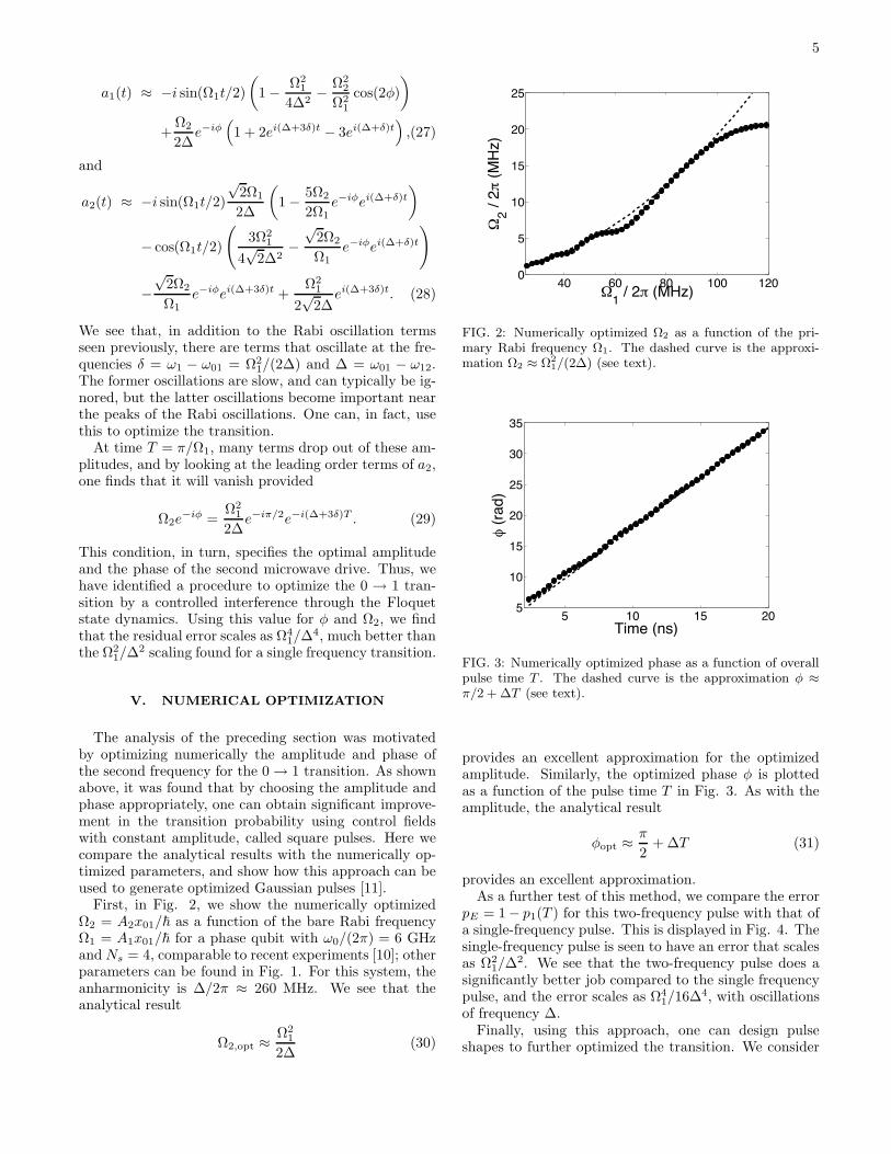
First, in Fig. 2, we show the numerically optimizedΩ2 = A2x01/~ as a function of the bare Rabi frequencyΩ1 = A1x01/~ for a phase qubit with ω0/(2π) = 6 GHzandNs = 4, comparable to recent experiments [10]; otherparameters can be found in Fig. 1. For this system, theanharmonicity is ∆/2π ≈ 260 MHz. We see that theanalytical result

Ω2,opt ≈Ω2

1

2∆(30)

FIG. 2: Numerically optimized Ω2 as a function of the pri-mary Rabi frequency Ω1. The dashed curve is the approxi-mation Ω2 ≈ Ω2

1/(2∆) (see text).

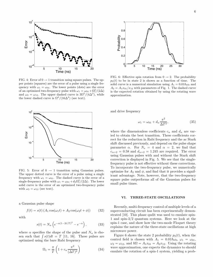
FIG. 3: Numerically optimized phase as a function of overallpulse time T . The dashed curve is the approximation φ ≈π/2 + ∆T (see text).

provides an excellent approximation for the optimizedamplitude. Similarly, the optimized phase φ is plottedas a function of the pulse time T in Fig. 3. As with theamplitude, the analytical result

φopt ≈π

2+ ∆T (31)

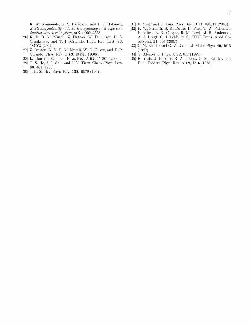
provides an excellent approximation.As a further test of this method, we compare the error

pE = 1− p1(T ) for this two-frequency pulse with that ofa single-frequency pulse. This is displayed in Fig. 4. Thesingle-frequency pulse is seen to have an error that scalesas Ω2

1/∆2. We see that the two-frequency pulse does a

significantly better job compared to the single frequencypulse, and the error scales as Ω4

1/16∆4, with oscillationsof frequency ∆.

Finally, using this approach, one can design pulseshapes to further optimized the transition. We consider

6

FIG. 4: Error of 0 → 1 transition using square pulses. The up-per points (squares) are the error of a pulse using a single fre-quency with ω1 = ω01. The lower points (dots) are the errorof an optimized two-frequency pulse with ω1 = ω01+Ω2

1/(2∆)and ω2 = ω12. The upper dashed curve is 3Ω2/(4∆2), whilethe lower dashed curve is Ω4/(16∆4) (see text).

FIG. 5: Error of 0 → 1 transition using Gaussian pulses.The upper dotted curve is the error of a pulse using a singlefrequency with ω1 = ω01. The dashed curve is the error of asingle-frequency pulse with ω1 = ω01 +d2Ω

2

1/(2∆). The lowersolid curve is the error of an optimized two-frequency pulsewith ω2 = ω12 (see text).

a Gaussian pulse shape

f(t) = s(t) (A1 cos(ω1t) +A2 cos(ω2t+ φ)) (32)

with

s(t) = Nα

(

e−α(1−2t/T )2 − e−α)

, (33)

where α specifies the shape of the pulse and Nα is cho-sen such that

∫

s(t)dt = T [11, 16]. These pulses areoptimized using the bare Rabi frequency

Ω1 =π

T

(

1 + cαπ2

(∆T )2

)

(34)

FIG. 6: Effective spin rotation from 0 → 2. The probabilityp2(t) to be in state 2 is shown as a function of time. Thesolid curve is a numerical simulation using A1 = 0.01~ω0 andA2 = A1x01/x12 with parameters of Fig. 1. The dashed curveis the expected rotation obtained by using the rotating waveapproximation.

and drive frequency

ω1 = ω01 + dαπ2

∆T 2, (35)

where the dimensionless coefficients cα and dα are var-ied to obtain the best transition. These coefficients cor-rect for the reduction in Rabi frequency and the ac Starkshift discussed previously, and depend on the pulse shapeparameter α. For Ns = 4 and α = 2, we find thatcα=2 = 0.58 and dα=2 = 1.245 are required. The errorusing Gaussian pulses with and without the Stark shiftcorrection is displayed in Fig. 5. We see that the single-frequency pulse is not effective without these corrections.To incorporate the two-frequency pulse, we numericallyoptimize for A2 and φ, and find that it provides a signif-icant advantage. Note, however, that the two-frequencysquare pulse outperforms all of the Gaussian pulses forsmall pulse times.

VI. THREE-STATE OSCILLATIONS

Recently, multi-frequency control of multiple levels of asuperconducting circuit has been experimentally demon-strated [10]. This phase qudit was used to emulate spin-1 and spin-3/2 quantum systems. Here we look at thespin-1 case, and show how the two-mode Floquet theoryexplains the nature of the three-state oscillations at highmicrowave power.

Figure 6 shows the state 2 probability p2(t), when thecontrol field is chosen with A1 = 0.01~ω0, ω1 = ω01,ω2 = ω12, and ~Ω = A1x01 = A2x12. Using the rotatingwave approximation, one expects the dynamics to shouldemulate the rotation of a spin-1 system, yielding a prob-

7

ability to be in state 2 of

p2(t) = sin4

(

Ωt

2√

2

)

. (36)

While it is expected that there may be Stark shifts, cor-rections to the Rabi frequencies, and off-resonant transi-tions for this square pulse, a qualitatively new effect isseen in the numerical simulation. This is a beating at the

frequency ∆ = ω1 − ω2.

Using the Floquet formalism, one finds that thedominant effect is a coupling between three photonblocks of the three-level system, or a total of ninestates: |0,−1, 1〉, |1,−2, 1〉, |2,−2, 0〉, |0, 0, 0〉, |1,−1, 0〉,|2,−1,−1〉, |0, 1,−1〉, |1, 0,−1〉, and |2, 0,−2〉. In thisbasis, the effective Hamiltonian is

HF = ~

−∆ Ω/2 0 0 12Ω/

√2 0 0 0 0

Ω/2 −∆ Ω/2 0 0 0 0 0 0

0 Ω/2 −∆ 0 Ω/√

2 0 0 0 0

0 0 0 0 Ω/2 0 0 12Ω/

√2 0

12Ω/

√2 0 Ω/

√2 Ω/2 0 Ω/2 0 0 0

0 0 0 0 Ω/2 0 0 Ω/√

2 00 0 0 0 0 0 ∆ Ω/2 0

0 0 0 12Ω/

√2 0 Ω/

√2 Ω/2 ∆ Ω/2

0 0 0 0 0 0 0 Ω/2 ∆

. (37)

Note that one 3-level block is isomorphic to a spin oper-ator for a spin-1 system.

By performing the lowest order of perturbation theoryfor the coupling between blocks of HF , one finds that therelevant transition amplitude is

a2(t) ≈ − sin2

(

Ωt

2√

2

)

− iΩ

4∆sin

(

Ωt√2

)

(1 + 2e−i∆t).

(38)This provides an excellent approximation to the beatingobserved in Fig. 6. Note that the perturbation, which isproportional to Ω/∆, happens to vanish precisely whenthe unperturbed oscillation reaches its maximum (t =√

2π/Ω.) Thus, it is likely that additional effects limitthis approach to a 0 → 2 transition. By extending thematrix to 15 states and higher orders in perturbationtheory, one finds a state 3 population proportional toΩ2/∆2.

VII. CONCLUSION

In this paper we have analyzed a set of multi-level ef-fects found in superconducting circuits such as the phaseor transmon qubit when controlled by pulses with twomicrowave frequencies. These involve a combination ofresonant, off-resonant, and interference effects that areof importance for future qubit (or qudit) superconduct-ing implementations of quantum information processors.Indeed, we have demonstrated that the many-mode Flo-quet formalism for multiple frequencies is a useful gener-alization of the standard rotating wave approximation.

First, we used the single-mode formalisim to recover

compact analytical results for corrections to Rabi oscil-lations in a three-level system, finding corrections to boththe resonance condition and the oscillation frequency ofrelative order Ω2/∆2. These are the ac Stark shift andreduction in Rabi frequency seen in existing experimentsand predicted previously.

Second, we have shown that simultaneously controllingthe qubit with two frequencies, one resonant with the 0 →1 transition (after compensating for the ac Stark shift)and the other resonant with the 1 → 2 transition leadsto a useful interference effect. This insight was inspiredby numerical results on square pulses, and found to be inexcellent agreement. This approach was further extendednumerically to show that two-frequency Gaussian pulsescan be developed for the 0 → 1 transition with significantimprovements over single-frequency pulses.

Finally, we have used the Floquet method to explainoff-resonant couplings that emerge when using the phasequdit to emulate a spin system. Here we have found andexplained a beating that is proportional to Ω/∆, andshould be observable in recent experiments, provided itis not masked by effects of decoherence.

In order for these effects to be genuinely useful, onewould like to extend the optimization of a transition be-tween two (or more) states to the optimization of a uni-tary operation acting an a superposition of these states.Here, however, an interesting difficulty emerges. For thesingle-frequency pulse, with square or Gaussian shapes,this is immediate: this control pulse is symmetric undertime-reversal: f(−t) = f(t). Consequently, the transi-tion from 0 → 1 and its time reverse from 1 → 0 areboth optimized for a single f(t). For the two-frequencypulse, however, f(−t) 6= f(t), and in fact the optimiza-

8

tion developed in Sec. III does not perform as well for the1 → 0 transition. Note that this observation sheds somelight on the two-quadrature approach of Ref. [16]: theclass of control pulses advocated there is time-reversalsymmetric. We expect that combining multiple quadra-tures and multiple frequencies will significantly expandthe control techniques for future experiments. Develop-ing simple, accurate, control pulses for multi-level quan-tum systems remains a challenging problem for theoryand experiment.

APPENDIX

In this appendix we summarize the perturbative resultsfor the cubic oscillator

H = ~ω0

(

1

2p2 +

1

2x2 − λx3

)

. (A.1)

Here we summarize the Rayleigh-Schrodinger perturba-tion expansion for the Hamiltonian H = H0 +λV . First,one expresses the n-th energy eigenstate, |Ψn〉, in powersof λ

|Ψn〉 =

∞∑

k=0

λk|n, k〉. (A.2)

In this expansion, |n, 0〉 is the n-th energy eigenstate ofH0, and |n, k〉 are the k-th order perturbative corrections.We also expand the energy eigenvalue in powers of λ,

En =∞∑

k=0

λkEn,k, (A.3)

where H0|n, 0〉 = En,0|n, 0〉. Substituting (A.2) and(A.3) in the eigenvalue equation

(H0 + λV )|Ψn〉 = En|Ψn〉, (A.4)

equating like powers of λk, and projecting onto 〈m, 0|allows one to solve for the energies and eigenfunctions:

En,k = 〈n, 0|V |n, k − 1〉 (A.5)

and

|n, k〉 =∑

m 6=n

〈m, 0|V |n, k − 1〉 −∑k−1j=1 En,j〈m, 0|n, k − j〉

En,0 − Em,0|m, 0〉. (A.6)

Extending this calculation to λ8 one finds

En/~ω0 = (n+ 1/2)− 1

8λ2(30n2 + 30n+ 11)− 15

32λ4(94n3 + 141n2 + 109n+ 31)

− 1

128λ6(115755n4 + 231510n3 + 278160n2 + 162405n+ 39709)

− 21

2048λ8(2282682n5 + 5706706n4 + 9387690n3 + 8374830n2 + 4244573n+ 916705). (A.7)

This procedure was implemented in Mathematica tocalculate the eigenvalues up to λ6; the λ8 expression(A.7) was found using a more efficient recursion-relationmethod [33], and agrees with [34] (provided one lets4N → 42N). These results, when compared with nu-

merical results found by complex scaling [35], are foundto be accurate for states n = 0 → 3 when Ns > 3.

In addition to the energy levels, perturbation theoryalso provides expressions for the wavefunctions. For ref-erence we list the third-order expression:

|Ψn〉 = |n〉 + λ

+3∑

k=−3

ak(n)|n+ k〉 + λ2+6∑

k=−6

bk(n)|n+ k〉 + λ3+9∑

k=−9

ck(n)|n+ k〉 (A.8)

9

where |n〉 = |n, 0〉 are the eigenstates of the purely harmonic oscillator Hamiltonian, and the nonzero expansioncoefficients are

a−3(n) = − 1

6√

2(n(n− 1)(n− 2))1/2 (A.9)

a−1(n) = − 3

2√

2n3/2 (A.10)

a+1(n) = − 3

2√

2(n+ 1)3/2 (A.11)

a+3(n) =1

6√

2((n+ 1)(n+ 2)(n+ 3))

1/2, (A.12)

b−6(n) =1

144(n(n− 1)(n− 2)(n− 3)(n− 4)(n− 5))

1/2(A.13)

b−4(n) =1

32(n(n− 1)(n− 2)(n− 3))

1/2(4n− 3) (A.14)

b−2(n) =1

16(n(n− 1))1/2 (7n2 − 19n+ 1) (A.15)

b+2(n) =1

16((n+ 1)(n+ 2))

1/2(7n2 + 33n+ 27) (A.16)

b+4(n) =1

32((n+ 1)(n+ 2)(n+ 3)(n+ 4))

1/2(4n+ 7) (A.17)

b+6(n) =1

144((n+ 1)(n+ 2)(n+ 3)(n+ 4)(n+ 5)(n+ 6))

1/2, (A.18)

and

c−9(n) = − 1

2592√

2(n(n− 1)(n− 2)(n− 3)(n− 4)(n− 5)(n− 6)(n− 7)(n− 8))

1/2(A.19)

c−7(n) = − 1

192√

2(n(n− 1)(n− 2)(n− 3)(n− 4)(n− 5)(n− 6))

1/2(2n− 3) (A.20)

c−5(n) = − 1

960√

2(n(n− 1)(n− 2)(n− 3)(n− 4))

1/2(80n2 − 305n+ 164) (A.21)

c−3(n) = − 1

1728√

2(n(n− 1)(n− 2))

1/2(488n3 − 2175n2 + 4018n− 825) (A.22)

c−1(n) = − 3

64√

2n1/2(20n4 + 81n3 + 326n2 + 81n+ 44) (A.23)

c+1(n) =3

64√

2(n+ 1)1/2(20n4 − n3 + 203n2 + 408n+ 228) (A.24)

c+3(n) =1

1728√

2((n+ 1)(n+ 2)(n+ 3))

1/2(488n3 + 3639n2 + 9832n+ 7506) (A.25)

c+5(n) =1

960√

2((n+ 1)(n+ 2)(n+ 3)(n+ 4)(n+ 5))

1/2(80n2 + 465n+ 549) (A.26)

c+7(n) =1

192√

2((n+ 1)(n+ 2)(n+ 3)(n+ 4)(n+ 5)(n+ 6)(n+ 7))1/2 (2n+ 5) (A.27)

c+9(n) =1

2592√

2((n+ 1)(n+ 2)(n+ 3)(n+ 4)(n+ 5)(n+ 6)(n+ 7)(n+ 8)(n+ 9))1/2 . (A.28)

One application of these expressions is to calculate the(properly normalized) matrix elements of the position op-

erator

xn,m =〈Ψn|x|Ψm〉

(〈Ψn|Ψn〉〈Ψm|Ψm〉)1/2. (A.29)

10

Using the wavefunctions (A.8) and matrix elements ofthe previous section, we find

x0,0 =3

2λ+

33

2λ3 (A.30)

x0,1 =

√2

2+

11√

2

8λ2 (A.31)

x0,2 = −√

2

2λ− 243

√2

16λ3 (A.32)

x0,3 =3√

3

8λ2 (A.33)

x1,1 =9

2λ+

213

2λ3 (A.34)

x1,2 = 1 +11

2λ2 (A.35)

x1,3 = −√

6

2λ− 405

√6

16λ3 (A.36)

x2,2 =15

2λ+

573

2λ3 (A.37)

x2,3 =

√6

2+

33√

6

8λ2 (A.38)

x3,3 =21

2λ+

1113

2λ3 (A.39)

with corrections of order λ4.

[1] J. M. Martinis, S. Nam, J. Aumentado, and C. Urbina,Phys. Rev. Lett. 89, 117901 (2002).

[2] J. M. Martinis, K. B. Cooper, R. McDermott, M. Stef-fen, M. Ansmann, K. D. Osborn, K. Cicak, S. Oh, D. P.Pappas, R. W. Simmonds, et al., Phys. Rev. Lett. 95,210503 (2005).

[3] I. Siddiqi, R. Vijay, M. Metcalfe, E. Boaknin, L. Frunzio,R. J. Schoelkopf, and M. H. Devoret, Phys. Rev. B 73,054510 (2006).

[4] F. Yoshihara, K. Harrabi, A. O. Niskanen, Y. Nakamura,and J. S. Tsai, Phys. Rev. Lett. 97, 167001 (2006).

[5] J. A. Schreier, A. A. Houck, J. Koch, D. I. Schuster,B. R. Johnson, J. M. Chow, J. M. Gambetta, J. Ma-jer, L. Frunzio, M. H. Devoret, et al., Phys. Rev. B 77,180502(R) (2008).

[6] A. A. Houck, J. A. Schreier, B. R. Johnson, J. M. Chow,J. Koch, J. M. Gambetta, D. I. Schuster, L. Frunzio,M. H. Devoret, S. M. Girvin, et al., Phys. Rev. Lett.101, 080502 (2008).

[7] R. Fazio, G. M. Palma, and J. Siewert, Phys. Rev. Lett.83, 5385 (1999).

[8] F. W. Strauch, P. R. Johnson, A. J. Dragt, C. J. Lobb,J. R. Anderson, and F. C. Wellstood, Phys. Rev. Lett.91, 167005 (2003).

[9] G. K. Brennen, D. P. O’Leary, and S. S. Bullock, Phys.Rev. A 71, 052318 (2005).

[10] M. Neeley, M. Ansmann, R. C. Bialczak, M. Hofheinz,E. Lucero, A. D. O’Connell, D. Sank, H. Wang, J. Wen-ner, A. N. Cleland, et al., Science 325, 722 (2009).

[11] M. Steffen, J. M. Martinis, and I. L. Chuang, Phys. Rev.B 89, 224518 (2003).

[12] M. H. S. Amin, Low Temp. Phys. 32, 198 (2006).[13] P. Rebentrost and F. K. Wilhelm, Phys. Rev. B 79,

060507(R) (2009).[14] S. Safaei, S. Montangero, F. Taddei, and R. Fazio, Phys.

Rev. B 79, 064524 (2009).[15] H. Jirari, F. W. J. Hekking, and O. Buisson, Europhys.

Lett. 87, 28004 (2009).[16] F. Motzoi, J. M. Gambetta, P. Rebentrost, and F. K.

Wilhelm, Phys. Rev. Lett. 103, 110501 (2009).[17] P. R. Johnson, F. W. Strauch, A. J. Dragt, R. C. Ramos,

C. J. Lobb, J. R. Anderson, and F. C. Wellstood, Phys.Rev. B 67, 020509 (2003).

[18] J. Koch, T. M. Yu, J. Gambetta, A. A. Houck, D. I.Schuster, J. Majer, A. Blais, M. H. Devoret, S. M. Girvin,and R. J. Schoelkopf, Phys. Rev. A 76, 042319 (2007).

[19] J. M. Chow, J. M. Gambetta, L. Tornberg, J. Koch,L. S. Bishop, A. A. Houck, B. R. Johnson, L. Frunzio,S. M. Girvin, and R. J. Schoelkopf, Phys. Rev. Lett. 102,090502 (2009).

[20] L. DiCarlo, J. M. Chow, J. M. Gambetta, L. S. Bishop,B. R. Johnson, D. I. Schuster, J. Majer, A. Blais, L. Frun-zio, S. M. Girvin, et al., Nature 460, 240 (2009).

[21] J. Claudon, F. Balestro, F. W. J. Hekking, and O. Buis-son, Phys. Rev. Lett. 93, 187003 (2004).

[22] J. Claudon, A. Zazunov, F. W. J. Hekking, and O. Buis-son, Phys. Rev. B 78, 184503 (2008).

[23] S. K. Dutta, F. W. Strauch, R. M. Lewis, K. Mitra,H. Paik, T. A. Palomaki, E. Tiesinga, J. R. Anderson,A. J. Dragt, C. J. Lobb, et al., Phys. Rev. B 78, 104510(2008).

[24] E. Lucero, M. Hofheinz, M. Ansmann, R. C. Bialczak,N. Katz, M. Neeley, A. O’Connell, H. Wang, A. N. Cle-land, and J. M. Martinis, Phys. Rev. Lett. 100, 247001(2008).

[25] M. A. Silanpaa, J. Li, K. Cicak, F. Altomare, J. I. Park,

11

R. W. Simmonds, G. S. Paraoanu, and P. J. Hakonen,Electromagnetically induced transparency in a supercon-

ducting three-level system, arXiv:0904.2553.[26] K. V. R. M. Murali, Z. Dutton, W. D. Oliver, D. S.

Crankshaw, and T. P. Orlando, Phys. Rev. Lett. 93,087003 (2004).

[27] Z. Dutton, K. V. R. M. Murali, W. D. Oliver, and T. P.Orlando, Phys. Rev. B 73, 104516 (2006).

[28] L. Tian and S. Lloyd, Phys. Rev. A 62, 050301 (2000).[29] T. S. Ho, S. I. Chu, and J. V. Tietz, Chem. Phys. Lett.

96, 464 (1983).[30] J. H. Shirley, Phys. Rev. 138, B979 (1965).

[31] F. Meier and D. Loss, Phys. Rev. B 71, 094519 (2005).[32] F. W. Strauch, S. K. Dutta, H. Paik, T. A. Palomaki,

K. Mitra, B. K. Cooper, R. M. Lewis, J. R. Anderson,A. J. Dragt, C. J. Lobb, et al., IEEE Trans. Appl. Su-percond. 17, 105 (2007).

[33] C. M. Bender and G. V. Dunne, J. Math. Phys. 40, 4616(1999).

[34] G. Alvarez, J. Phys. A 22, 617 (1989).[35] R. Yaris, J. Bendler, R. A. Lovett, C. M. Bender, and

P. A. Fedders, Phys. Rev. A 18, 1816 (1978).