Ultrasonics 42 (2004) 813–818

www.elsevier.com/locate/ultras

On estimating the center frequency of ultrasonic pulses

L. Vergara a,*, J. Gos�albez a, R. Miralles a, I. Bosch a

a ETSI Telecomunicaci�on, Univesidad Polit�ecnica de Valencia, Camino de Vera s/n, Valencia 46022, Spain

Abstract

In this paper we propose a new technique for estimating the center frequency of the ultrasound pulse from records of back-

scattering noise. We start by considering that the conventional maximum frequency method can be seen as a filtering (differentiator)

of the pulse spectrum magnitude followed by a searching for the zero-crossing value. The new approach replaces the differentiator by

a Hilbert transformer. We show in the paper that the proposed method has less variance than the maximum frequency method. In

particular, we analyse the performance assuming that the real cepstrum method is used for extracting pulse spectrum magnitude. We

give an upper bound for the variance reduction when practical criteria are applied for fitting the cepstrum cut-off frequency. The

analytical work is verified by real and simulated data.

� 2004 Elsevier B.V. All rights reserved.

Keywords: Backscattering noise; Real cepstrum; Center frequency; Variance

1. Introduction

Tracking of the center frequency of the ultrasound

pulse is required in different applications of nonde-

structive evaluation of materials and tissues by ultra-

sonic backscattering noise analysis. If the attenuation

may be considered to be linearly dependent on fre-quency, the center frequency estimates are used for

estimating the attenuation coefficient [1–4]. In other

cases the center frequency estimates are correlated with

properties of material [5–7], or for flaw detection [8].

There are different alternatives for computing the

center frequency. Zero-crossing counting [1,2] is a time

domain technique. It is attractive from the point of view

of simplicity, but it is not adequate for short records(low-resolution) and/or low signal-to-noise ratio condi-

tions. Frequency domain methods are based in a pre-

vious spectral analysis for pulse spectrum magnitude

(PSM) extraction [4,9–13]. Once we have the PSM, the

centroid frequency may be computed and then consid-

ered to be a center frequency estimate but some bias is

unavoidable due to integration band.

The problem of bias is not present if the center fre-quency is estimated by means of the maximum [4,7,8] of

*Corresponding author. Tel.: +34-96-3877308; fax: +34-96-

38773919.

E-mail address: lvergara@dcom.upv.es (L. Vergara).

0041-624X/$ - see front matter � 2004 Elsevier B.V. All rights reserved.

doi:10.1016/j.ultras.2004.01.057

the PSM, because no integration band is required.

Additionally the background noise problem is less

important, as the maximum is located at the highest

signal to noise ratio band of the spectrum.

In Section 2 of this paper, we present a filtering ap-

proach to compute the maximum frequency and its

variance. In Section 3, a new method is proposed, wherefurther variance reduction is possible. It is based on

using a Hilbert transformer. In Section 4 we consider the

case of using the real cepstrum method. We arrive to an

upper bound for the variance reduction that could be

obtained. Finally, in Section 5 we present simulated and

real data analysis to verify the usefulness and limitations

of new method.

2. A filtering approach to compute the maximum

frequency

Let us consider the analytic representation of the

ultrasonic pulse

uðtÞ ¼ qðtÞejxct ð1Þwhere qðtÞ is the envelope and xc ¼ 2pfc the centerpulsation. Fourier transform of uðtÞ is (2)UðxÞ ¼ Qðx � xcÞ ð2ÞThe problem is that of building estimates of xc from

estimates of jUðxÞj. Different techniques have been

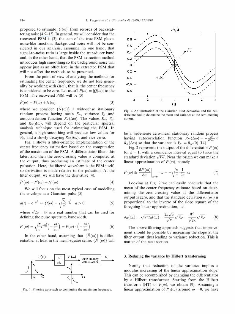
Fig. 2. An illustration of the Gaussian PSM derivative and the heu-

ristic method to determine the mean and variance at the zero-crossing

output.

814 L. Vergara et al. / Ultrasonics 42 (2004) 813–818

proposed to estimate jUðxÞj from records of backscat-

tering noise [4,9–13]. In general, we will consider that the

recovered PSM is (3), the sum of the true PSM plus a

noise-like function. Background noise will not be con-

sidered in our analysis, assuming, in one hand, thatsignal-to-noise ratio is large inside the transducer band

and, in the other hand, that the PSM extraction method

introduces high smoothing so the background noise will

appear just as an offset level in the extracted PSM that

will not affect the methods to be presented.

From the point of view of analysing the methods for

estimating the center frequency, we do not lose gener-

ality by working with QðxÞ, that is, the center frequencyis considered to be zero. Let us call P ðxÞ ¼ jQðxÞj to thePSM. The recovered PSM will be (3)

P̂ ðxÞ ¼ PðxÞ þ NðxÞ ð3Þwhere we consider feN ðxÞg a wide-sense stationary

random process having mean EN , variance VN and

autocorrelation function RNðDxÞ. The values EN , VN ,and RN ðDxÞ, will depend on the particular spectral

analysis technique used for estimating the PSM. In

general, a high smoothing will produce low values for

VN , and a slowly decaying RN ðDxÞ, and vice versa.Fig. 1 shows a filter-oriented implementation of the

center frequency estimation based on the computation

of the maximum of the PSM. A differentiator filters this

later, and then the zero-crossing value is computed atthe output, thus producing an estimate of the center

pulsation. Here, the filtered waveform is the PSM itself,

so derivation is made relative to the pulsation. At the

filter output, we will have the derivative (4).

P̂ 0ðxÞ ¼ P 0ðxÞ þ N 0ðxÞ ð4ÞWe will focus on the most typical case of modelling

the envelope as a Gaussian pulse (5)

qðtÞ ¼ e�at2 $ QðxÞ ¼ffiffiffipa

re�

x24a a > 0 ð5Þ

whereffiffiffiffiffi2a

p¼ W is a real number that can be used for

defining the pulse spectrum bandwidth.

P 0ðxÞ ¼ffiffiffipa

re�

x24a

�� x2a

�¼ P ðxÞ �

�� x2a

�ð6Þ

In the other hand, assuming that feN ðxÞg is differ-entiable, at least in the mean-square sense, feN 0ðxÞg will

Fig. 1. Filtering approach to computing the maximum frequency.

be a wide-sense zero-mean stationary random process

having autocorrelation function RN 0 ðDxÞ ¼ � d2

dDx2 RN ðDxÞ so that the variance is VN 0 ¼ RN 0 ð0Þ [14].Fig. 2 represents the output of the differentiator P 0ðxÞ

for a ¼ 1, with a confidence interval equal to twice the

standard deviationffiffiffiffiffiffiffiVN 0

p. Near the origin we can make a

linear approximation of P 0ðxÞ, namely

P 0ðxÞ ffi dP 0ðxÞdx

����x¼0

� x ¼ �ffiffiffipa

r� 12a

� x ð7Þ

Looking at Fig. 2 we can easily conclude that the

mean of the center frequency estimate based on deter-

mining the zero-crossing value at the differentiatoroutput is zero, and that the standard deviation rDðx̂cÞ isproportional to the inverse of the slope square of the

foregoing linear approximation, i.e.,

rDðx̂cÞ ¼ffiffiffiffiffiffiffiffiffiffiffiffiffiffiffiffiffiffivarDðx̂cÞ

p¼ 2a

ffiffiffia

pffiffiffip

pffiffiffiffiffiffiVN 0

p¼ W 3ffiffiffiffiffiffi

2pp

ffiffiffiffiffiffiVN 0

pð8Þ

The above filtering approach suggests that improve-

ment should be possible by increasing the slope at the

filter output, thus leading to variance reduction. This is

matter of the next section.

3. Reducing the variance by Hilbert transforming

Noting that reduction of the variance implies a

modulus increasing of the linear approximation slope.

This can be accomplished by changing the differentiator

by a Hilbert transformer. Starting from the Hilbert

transform (HT) of PðxÞ, we obtain (9). Assuming alinear approximation of PHðxÞ around x ¼ 0, we have

L. Vergara et al. / Ultrasonics 42 (2004) 813–818 815

to compute the derivative. For the Gaussian envelope

pulse, this leads to Eq. (10).

PHðxÞ ¼ HT½P ðxÞ� ¼ 2

Z 1

0

Re½pðtÞ� sinðxtÞdt

¼ P ðxÞerf x2

ffiffiffia

p

ð9Þ

P 0HðxÞ

��x¼0 ¼ 2

Z 1

0

Re½pðtÞ�t cosðxtÞdt����x¼0

¼ 1

að10Þ

This value indicates that, by using a Hilbert trans-

former, the variance of the center frequency estimatebased on computing the zero-crossing point at the out-

put of the filter, will be proportional to a2 instead of toa3 as in (8).Making a similar analysis to the one made in Section

2 we obtain (11). Let us call P̂HðxÞ to the extracted PSMfiltered by the Hilbert transformer, so that

P̂HðxÞ ¼ PHðxÞ þ NHðxÞ ð11Þwhere P̂HðxÞ is the extracted PSM filtered by the Hilbert

transformer. PHðxÞ and NHðxÞ are, respectively the re-sponses of the Hilbert transformer to the true PSM and

to the distortion noise-like contribution. Relative to

NHðxÞ, it will be a wide-sense stationary random pro-

cess. The Hilbert transformer impulse respond is odd, so

the mean value of NHðxÞ will be zero. The magnitude ofits frequency response equals one, so that VNH ¼ VN .In Fig. 3 we have represented together �PHðxÞ and

P 0ðxÞ (we change the sign for a better comparison). Theslope is increased by means of using the Hilbert trans-

form filter.

Now, following a similar heuristic approach to the

one used for finding (8) and using Eq. (10), we can

determine the standard deviation rHðx̂cÞ of the center

Fig. 3. Comparison of the Gaussian PSM derivative and the Gaussian

PSM Hilbert transform for a ¼ 4.

pulsation estimate at the output of the Hilbert trans-

former by means of

rHðx̂cÞ ¼ffiffiffiffiffiffiffiffiffiffiffiffiffiffiffiffiffiffiffivarHðx̂cÞ

p¼ a

ffiffiffiffiffiffiffiVNH

p¼ a

ffiffiffiffiffiffiVN

p¼ W 2

2

ffiffiffiffiffiffiVN

pð12Þ

With the aim of comparing both estimators we may

define the improvement ratio (13).

r ¼ rDðx̂cÞrHðx̂cÞ

¼ffiffiffi2

p

rW

ffiffiffiffiffiffiVN 0

VN

rð13Þ

The variance quotient VN 0=VN will depend on the

particular method applied for the PSM extraction. In

the next section we present an approximate expression

for r for the particular, but very usual, case of applyingthe real cepstrum method for extracting the PSM.

4. Application to the real cepstrum method

Real cepstrum method [9,12] may be summarised in

Eq. (14).

P̂ ðxÞ ¼ expðILPLhlnðjX ðxÞjÞiÞ ð14Þ

where X ðxÞ is the Fourier transform of the grain noise

record under analysis. ILPL indicates ideal low-pass

liftering which allows separation of the PSM logarithm.

We have deduced an approximate expression for r,under the two following assumptions:

• X ðxÞ ¼ PðxÞW ðxÞ, where f eW ðxÞg, the multiplica-tive noise due to the reflectivity is an independent

wide-sense stationary stochastic process.

• The cut-off quefrency of the ILPL is high enough to

allow the PSM not to be perturbed.

The approximation is (15)

r ffiffiffiffiffiffiffi2

3p

rW � c ð15Þ

where c is the cut-off quefrency used for implementingthe ILPL. The Eq. (15) indicates that the improving

factor linearly depends on the time-bandwidth product

W � c. Actually, W and c will not be independent valuesin practice. Noting that increasing c implies increasingboth VN and VN 0 , and so increasing the center frequency

variance of both methods, we should use the minimum

value of c compatible with the hypothesis of the PSMnot being affected by the ILPL. We consider c mustequal the inverse of the separation bandwidth between

the two frequencies where the pulse spectrum log-mag-

nitude reaches respectively the 10% and the 90% of the

maximum value [9]. For the Gaussian pulse case, this

implies (16). From Eq. (15) and for those cases where

this practical criterium is used, we obtain (17)

816 L. Vergara et al. / Ultrasonics 42 (2004) 813–818

� f 20:12 W

2p

� �2 ¼ 0:1 � f 20:92 W

2p

� �2 ¼ 0:9

) c ¼ 1

f0:1 � f0:9¼ 1:118

2pW

ð16Þ

r ffi 1:118 �ffiffiffiffiffiffi8p3

r¼ 3:236 ð17Þ

In the next section we will verify by simulated and

real data analysis the validity of Eq. (17) and some

limitations that may appear due to the discrete-time

processing.

5. Data analysis

In this section we present the results corresponding to

estimation of the center frequency by using the two

methods considered. We start by considering some real

data analysis corresponding to backscattering ultrasonic

noise recorded in a cement paste probe. The probe is aprism of a size 16 · 4 · 4 (cm3), water-cement ratio was

40%. Other data are

• Pulser-receiver: IPR-100, Physical acoustics

• Transducers: KBA-10 MHz, KBA-5 MHz

• Digitalisation: Tektronix TDS-3012

• Sampling frequency: 250 MHz

• Number of records: 20 at different locations

First of all, we must take into account that the deri-

vations of the foregoing sections have been made in

continuous-time domain, while here we are going to

make a digital processing of the data. Another impor-

tant aspect is having enough resolution in the frequency

domain, because we are going to filter the extracted

PSM as actual waveforms.The pulse time-duration is proportional to the inverse

of the bandwidth W and the sampling period in the

pulsation domain is ð2p=LÞfs, where L is the FFT-size

used for computing the Fourier transforms in (14) and fsis the sampling frequency in time domain. So we obtain

(18)

L2p � fs

P 2 � K � 1W

) LP 2 � K 1

W =ð2pfsÞð18Þ

Table 1

Center frequency estimates for both methods and improvement factors, usin

Record length ftransducer ¼ 5 MHz

Westimated ¼ 1:8 MHz, fs ¼ 31:25 MHz

f̂D � r̂D (MHz) f̂H � r̂H (MHz) r

256 5.83± 0.94 5.60± 0.61 1.54

512

where K is a constant greater than 1, large enough to

make it possible neglecting overlapping effects. We

should obtain a normalised bandwidth as large as pos-

sible. For the 5 MHz cement paste data we have deci-

mated the original 250 MHz sampled records by a factorof 8, so we have fs ¼ 31:25 MHz. Similarly, for the 10MHz cement paste data we have decimated the original

records by a factor of 4, so we have fs ¼ 62:5 MHz.Both values seem to be adequate trade-offs. In both

cases we started from a data interval of 2048 samples

ranging from an approximate depth of 0.2 cm to a depth

of 1.53 cm, into the material. This interval defines a

practical range between too near data where transientresponse of the transmitter is present, and too far data

where backscattering noise is under the background

noise level.

Before applying the methods we need a raw estimate

of W , so we can define the cepstrum cut-off c. It havebeen calculated that the raw estimates for W are

2p 1:8 106 rad s�1 for the 5 MHz case and 2p 1:25 106 rad s�1 for the 10 MHz case. With that valuesand using Eq. (16) we obtain (19). Nc5MHz and Nc10MHzare the cepstrum cut-off frequencies used in the discrete-

time implementation of the real cepstrum domain

method for pulse extraction.

Nc5MHz ¼c5MHz

Tsffi 19 ð19aÞ

Nc10MHz ¼c10MHz

Tsffi 56 ð19bÞ

In Table 1 we show the results obtained with the real

data analysis. The indicated values are the mean and the

standard deviation for the 20 center frequency estimates

computed with each method. Looking at Fig. 4a, we see

that the center of the bandwidth is above 5 MHz, so we

can hardly say that this is a 5 MHz transducer. Fig. 4b

corresponds to 10 MHz transducer example. In any

case, a significant improvement is obtained with HilbertTransformer case. For 5 MHz transducer, a variance

reduction by a factor of r2 ¼ 2:38 is obtained, and forthe 10 MHz case the reduction is by a r2 ¼ 2:04 factor.To overcome the maximum available record length

constraint, we have made some simulations, using the

same values to those corresponding to the real data case.

The backscattering noise was simulated by convolution

of a Gaussian envelope pulse with a random Gaussian

g real data

ftransducer ¼ 10 MHz

Westimated ¼ 1:25 MHz, fs ¼ 62:5 MHz

f̂D � r̂D (MHz) f̂H � r̂H (MHz) r

10.16± 0.61 10.03± 0.43 1.43

Fig. 4. Real data mean spectra used for estimating the bandwidth W : (a) 5 MHz case and (b) 10 MHz case.

Table 2

Center frequency estimates for both methods and improvement factors, using simulated data

Record length ftransducer ¼ 5 MHz ftransducer ¼ 10 MHz

Westimated ¼ 1:8 MHz, fs ¼ 31:25 MHz Westimated ¼ 1:25 MHz, fs ¼ 62:5 MHz

f̂D � r̂D (MHz) f̂H � r̂H (MHz) r f̂D � r̂D (MHz) f̂H � r̂H (MHz) r

256 5.78± 0.74 5.75± 0.49 1.51 10.00±0.623 10.01± 0.45 1.396

512 5.69± 0.59 5.74± 0.31 1.893 9.97±0.512 9.99± 0.34 1.497

2048 5.739± 0.424 5.71± 0.15 2.79 10.03±0.363 10.01± 0.18 2.0166

8192 5.73± 0.25 5.71± 0.08 2.928 9.98±0.248 9.99± 0.09 2.725

16384 5.69± 0.19 5.71± 0.06 3.113 10.00±0.19 10.00± 0.07 2.785

L. Vergara et al. / Ultrasonics 42 (2004) 813–818 817

and independent reflectivity sequence. The number of

runs was 200 to have enough reliability. The main re-

sults are summarised in Table 2 and following signifi-

cant conclusions are derived:

• The center frequency estimates are unbiased in both

methods

• We obtain less variance in the Hilbert transformermethod (r > 1) in all the cases

• Values of r are similar to the real data when the re-cord lengths were similar

• Improvement factor r converges towards theoreticallimit 3.236 as record length grows

All the above conclusions verify that the assumed

hypothesis and approximations are reasonable andvalidate the analytical results derived in the previous

sections.

6. Conclusions

We have proposed a new method to estimate ultra-

sound center frequency that is able to reduce the vari-ance. It is based on using a Hilbert transformer instead

of a differentiator to filter the PSM extracted from the

backscattering noise records.

We have presented analytical work showing the terms

affecting the variance (8) and (12), where the bandwidth

has an important influence. However the actual variance

reduction is also dependent on the particular method

applied for PSM extraction. Thus we have concentrated

on the widely used real cepstrum method. For that case,

we have deduced that the actual improvement is

dependent on the time-bandwidth product, where timemeans the cut-off frequency used in the cepstrum do-

main. Applying the practical method of Eq. (16) for

fitting the cut-off frequency, we found an approximate

upper bound for the improvement factor, which implies

that a variance reduction of (3.236)2 ¼ 10.47 could be

obtained.

To reach the above reduction we must have long

enough records. In any case we have shown by real andsimulated data analysis that significant variance reduc-

tion may be obtained even working with records much

shorter than those ones necessary to reach the upper

bound.

Acknowledgements

This work has been supported by Spanish Adminis-

tration under grant TIC 2002/04643.

818 L. Vergara et al. / Ultrasonics 42 (2004) 813–818

References

[1] R. Kuc, Processing of diagnostic ultrasound signals, IEEE Acous.

Speech Signal Process. Mag. (1984) 19–26.

[2] R. Kuc, Estimating acoustic attenuation from reflected ultrasound

signals: comparison of spectral-shift and spectral––difference

approaches, IEEE Trans. Acous. Speech Signal Process. 32

(1984) 1–6.

[3] T. Baldeweck, A. Laugier, A. Herment, G. Berger, Application of

autoregressive spectral analysis for ultrasound attenuation esti-

mation: interest in highly attenuating medium, IEEE Trans.

Ultrason. Ferroelect. Freq. Control 42 (1995) 99–109.

[4] J.M. Girault, F. Ossant, A. Ouahabi, D. Kouam�e, F. Patat, Time-

varying autoregressive spectral estimation for ultrasound attenu-

ation in tissue characterisation, IEEE Trans. Ultrason. Ferroelect.

Freq. Control 45 (1998) 650–659.

[5] J. Saniie, N.M. Bilgutay, T. Wang, Signal processing of ultrasonic

backscattered echoes for evaluating the microstructure of mate-

rials, in: C.H. Chen (Ed.), Signal Processing and Pattern Recog-

nition in Nondestructive Evaluation of Materials, Springer-

Verlag, Berlin, 1988, pp. 87–100.

[6] J. Saniie, T. Wang, N.M. Bilgutay, Analysis of homomorfic

processing for ultrasonic grain signals, IEEE Trans. Ultrason.

Ferroelect. Freq. Control 36 (1989) 365–375.

[7] T. Wang, J. Saniie, Analysis of low-order autoregressive mod-

els for ultrasonic grain noise characterization, IEEE Trans.

Ultrason. Ferroelect. Freq. Control 38 (1991) 116–124.

[8] J. Saniie, X.M. Jin, Spectral analysis for ultrasonic nondestructive

evaluation applications using autoregressive, Prony, and multiple

signal classification methods, J. Acoust. Soc. Am. 100 (1996)

3165–3171.

[9] J.A. Jensen, Estimation of pulses in ultrasound B-scan images,

IEEE Trans. Med. Imaging 10 (1991) 164–172.

[10] K.B. Rasmussen, Maximum likelihood estimation of the attenu-

ated ultrasound pulse, IEEE Trans. Signal Process. 42 (1994) 220–

222.

[11] J.A. Jensen, Nonparametric estimation of ultrasound pulses,

IEEE Trans. Biomed. Eng. 10 (1994) 929–936.

[12] T. Taxt, Comparison of cepstrum-based methods for radial blind

deconvolution of ultrasound images, IEEE Trans. Ultrason.

Ferroelect. Freq. Control 44 (1997) 666–674.

[13] U.R. Abeyratne, A.P. Petropulu, J.M. Reid, Higher order

spectra based deconvolution of ultrasound images, IEEE

Trans. Ultrason. Ferroelect. Freq. Control 42 (1995) 1063–

1075.

[14] A. Le�on-Garc�ıa, Probability and Random Processes for Electrical

Engineering, Addison-Wesley, Reading, MA, 1994.