Rigorous asymptotic expansions for Lagerstrom’s model

equation—a geometric approach

Nikola Popovic∗ Peter Szmolyan∗

July 17, 2004

Abstract

The present work is a continuation of the geometric singular perturbation anal-ysis of the Lagerstrom model problem which was commenced in [PS04]. Weestablish the same framework here, reinterpreting Lagerstrom’s equation as adynamical system which is subsequently analyzed by means of methods fromdynamical systems theory as well as of the blow-up technique. We show howrigorous asymptotic expansions for the Lagerstrom problem can be obtainedusing geometric methods, thereby establishing a connection to the method ofmatched asymptotic expansions. We explain the structure of these expansionsand demonstrate that the occurrence of the well-known logarithmic (switchback)terms therein is caused by a resonance phenomenon.

1 Introduction

Singular perturbation problems in general and singularly perturbed differential equa-tions in particular are characterized by the presence of at least two fundamentallydifferent scales. The existence of these independent scales gives one a small para-meter and thus permits one to use perturbation methods. The aim of these methodsis to obtain uniformly valid approximations. It is, however, the essence of a singu-lar perturbation problem that a straightforward perturbation fails to be uniformlyvalid. Indeed, it is typical of singular perturbation techniques that one works withapproximations which are valid in restricted domains only.

Traditionally, this type of problems has been treated using the method of matchedasymptotic expansions: one proceeds by constructing two (or more) asymptotic ex-pansions which together cover the entire domain, although neither is uniformly validthere. To obtain a uniformly valid approximation on the entire domain, these indi-vidual expansions have to be matched; the essence of matching lies in comparing twoexpansions on a suitable domain of overlap. An excellent account of the fundamentalnotions and concepts in perturbation theory is given in [LC72].

∗Institute for Analysis and Scientific Computing, Vienna University of Technology, WiednerHauptstraße 8-10, A-1040 Vienna, Austria, EU.

1

More recently, an alternative approach to such problems, known as geometricsingular perturbation theory, has emerged (see [Fen79] or [Jon95] for details and ref-erences). This approach, which in general requires certain hyperbolicity assumptions,is based on methods from the theory of dynamical systems, in particular on invariantmanifold theory.

A classical singular perturbation problem from fluid dynamics occurs in theasymptotic treatment of viscous flow past a solid at low Reynolds number, see e.g.[vD75]. Though first attempts at clarification date back to [Sto51], it was not untila century later that the conceptual structure of the problem was at last resolved in[Kap57], [KL57], and [PP57]. To illustrate the mathematical ideas and techniquesused by Kaplun in his asymptotic treatment of low Reynolds number flow, [Lag66]proposed an analytically rather simple model problem which was subsequently ana-lyzed by Lagerstrom himself as well as by numerous other workers, see [Lag88] andthe references therein.

Much of the interest in Lagerstrom’s model problem has been directed at thedevelopment of matched asymptotic expansions to describe its solutions, see e.g.[KC81], [Lag88], or [HTB90]. Our goal is to show how such expansions can beobtained using geometric methods, thereby establishing a connection between thetwo approaches. As observed already by [Fen79], for layer-type problems findingouter solutions is equivalent to computing expansions of slow manifolds. However,the well-developed geometric theory is not applicable at points where hyperbolicityis lost. In several instances it has been possible to extend the geometric approachpast such points using the blow-up technique. Blow-up is essentially a sophisticatedrescaling which allows one to analyze the dynamics near a singularity; details can befound in [DR96]. In particular, blow-up has been employed by [KS01] and [vGKS] togive a detailed geometric analysis of the singularly perturbed planar fold. Apart fromderiving asymptotic expansions of slow manifolds continued beyond the fold point,they also explained the structure of these expansions and gave an algorithm for thecomputation of its coefficients. Our line of attack is very similar to theirs.

A distinctive feature of asymptotic expansions for the singularly perturbed planarfold as well as for Lagerstrom’s model is the occurrence of logarithmic terms. Thenature of the expansions in these and similar problems is both complicated and un-expected, as the governing equations typically give no immediate hint of the presenceof such terms; indeed, this is why they are often so tricky to obtain. Traditionally,logarithmic terms have been accounted for under the notions of switchback and in-tegrated effects. We show that the occurrence of logarithms in the expansions forLagerstrom’s model equation is caused by a resonance phenomenon. At this pointwe conjecture that similar resonance phenomena are responsible for the occurrenceof logarithmic terms in many other singular perturbation problems, at least afterreinterpretation in a dynamical systems framework.

This article is organized as follows: Section 2 contains some background informa-tion on the Lagerstrom model problem as well as on the blow-up transformation usedin our analysis; in Section 3 we derive asymptotic expansions for Lagerstrom’s model,

2

whereas Section 4 briefly indicates how these expansions are related to the classicalones known from the literature. This work should be regarded as a continuation of[PS04].

2 Background information

2.1 Lagerstrom’s model equation

In its simplest form, Lagerstrom’s model equation is given by the non-autonomoussecond-order boundary value problem

u +n − 1

xu + uu = 0 (2.1a)

u(ε) = 0, u(∞) = 1 (2.1b)

with n ∈ N, 0 < ε ≤ x ≤ ∞, and the overdot denoting differentiation with respectto x. Equivalently, by introducing the rescaling

ξ =x

ε, (2.2)

one can write (2.1) as

u′′ +n − 1

ξu′ + εuu′ = 0 (2.3a)

u(1) = 0, u(∞) = 1 (2.3b)

with 1 ≤ ξ ≤ ∞ and the prime denoting differentiation with respect to ξ.Originally, (2.1) and (2.3) are the versions of the model which was first intro-

duced in [Lag66] and [KL57] to elucidate certain basic ideas used in the asymptotictreatment of viscous flow past a solid at low Reynolds number. In the followingwe will only consider the cases n = 2 and n = 3, which represent the physicallyrelevant settings of flow in two and three dimensions, respectively. For more back-ground information and further references on Lagerstrom’s model equation we referto [PS04].

As in [PS04], replacing ξ ∈ [1,∞) by η := ξ−1 ∈ (0, 1], appending the (trivial)equation ε′ = 0, and setting u′ = v yields

u′ = v

v′ = −(n − 1)ηv − εuv

η′ = −η2

ε′ = 0

(2.4)

in extended phase space, with boundary conditions given by

u(1) = 0, η(1) = 1, u(∞) = 1; (2.5)

3

Wssε

Wcε

u

η

v

Vε

Q

Wsε

vε

Mε

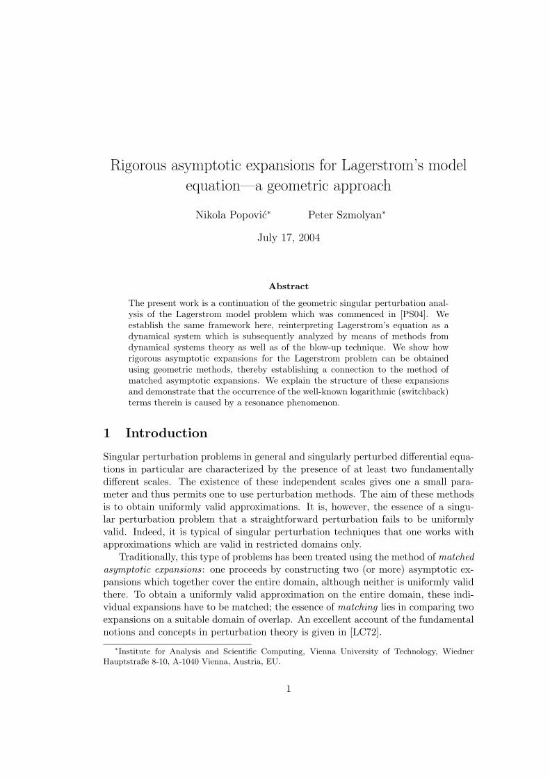
Figure 1: Geometry of system (2.4) for ε > 0 fixed.

obviously, (2.5) means that v(∞) = 0 for the solution to (2.4), whereas v(1) still isto be determined.

For ε > 0 fixed, let Vε be defined by

Vε := {(0, v, 1)| v ∈ [v, v]}, (2.6)

where 0 ≤ v < v < ∞, and let the point Q be given by Q := (1, 0, 0) (see again[PS04]). Note that Vε and Q correspond to the inner and outer boundary conditionsin (2.3b), respectively. The saturation of Vε under the flow induced by (2.4) we denoteby Mε. Correspondingly, the manifolds V and M in extended phase space are definedby V :=

⋃

ε∈[0,ε0] Vε × {ε} and M :=⋃

ε∈[0,ε0] Mε × {ε}; here the parameter ε is notfixed, but is allowed to vary in some interval [0, ε0] with ε0 > 0 small.

The equilibria of (2.4) are located on the line l := {(u, v, η, ε)| u ∈ R+, v = η =

ε = 0}; obviously, Q ∈ l. For ε > 0, the one-dimensional strongly stable manifoldof Q, which we call Wss

ε , can be computed explicitly due to the simple structure of(2.4) for η = 0, whence e.g.

v(u) =ε

2

(

1 − u2)

; (2.7)

here we have used v(1) = 0. The following result can be found in [PS04]:

Proposition 2.1 ([PS04]). Let k ∈ N be arbitrary, and let ε > 0.

4

1. There exists an attracting two-dimensional center manifold W cε of (2.4) which

is given by {v = 0}.

2. For |u − 1|, v, and η sufficiently small, there is a stable invariant Ck-smoothfoliation Fs

ε with base Wcε and one-dimensional Ck-smooth fibers.

Given Proposition 2.1, one can define the stable manifold Wsε of Q as

Wsε :=

⋃

P∈Υ

F sε (P ), (2.8)

where Υ := {(1, 0, η)| 0 ≤ η � 1}, i.e., as a union of fibers F sε ∈ Fs

ε with base pointsin the weakly stable orbit Υ. The situation is illustrated in Figure 1.

The main result in [PS04] is the following theorem on the existence and (local)uniqueness of solutions to (2.4) (and, consequently, to (2.1)):

Theorem 2.1 ([PS04]). For ε ∈ (0, ε0] with ε0 > 0 sufficiently small and n = 2, 3,there exists a locally unique solution to (2.4),(2.5).

The proof is constructive, and is performed by tracking Mε through phase spaceand showing that its intersection with Ws

ε is transverse under the resulting flow.As we are only interested in small values of ε, we took a perturbational approach:given transversality for ε = 0, we concluded that the intersection remained transversefor ε > 0 small. On a technical level, the tracking was done along singular orbitsof (2.4) connecting V0 to Q. These orbits, which we denoted by Γ, were used astemplates for orbits of the full problem obtained for ε > 0. However, due to thenon-hyperbolic character of the problem for ε = 0, we could not deduce the existenceof a stable manifold Ws

0 from standard invariant manifold theory. It was shown in[PS04], however, that Wss and Ws can still be smoothly defined down to ε = 0 byusing blow-up techniques.

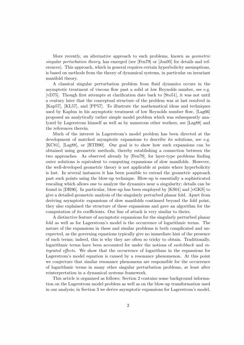
2.2 The blow-up transformation

The (polar) blow-up transformation Φ introduced in [PS04] to analyze the dynamicsof (2.4) near l is given by

Φ :

{

R × B → R4

(u, v, η, ε, r) 7→ (u, rv, rη, rε),(2.9)

where B := S2 × R and S

2 denotes the two-sphere in R3, i.e., S

2 ={

(v, η, ε)∣

∣ v2 +η2 + ε2 = 1

}

. Note that obviously Φ−1(l) = R × S2 × {0}, which is the blown-up

locus obtained by setting r = 0. Moreover, for r 6= 0, i.e., away from Φ−1(l), Φ is aC∞-diffeomorphism. We will only be interested in r ∈ [0, r0] with r0 > 0 small.

The reason for introducing (2.9) is that degenerate equilibria, such as those in l,are often amenable to analysis by means of blow-up techniques. The blow-up is a(singular) coordinate transformation whereby the degenerate equilibrium is blown up

5

K1

K2

ε

Φ−1

u, v

ε

u, v

ηη

Φ

Figure 2: The blow-up transformation Φ.

to some n-sphere. Transverse to the sphere and even on the sphere itself one oftengains enough hyperbolicity to allow a complete analysis by standard techniques. For ageneral discussion of blow-up we refer to [DR91] and to [Dum93], whereas applicationsto singular perturbation problems can be found in [DS95] and [DR96] as well as in[KS01] and [vGKS].

The vector field on R × B, which is induced by the vector field corresponding to(2.4), is most conveniently studied by introducing different charts for the manifoldR × B. In the following, we will be concerned only with two charts K1 and K2

corresponding to η > 0 and ε > 0 in (2.9), respectively, see Figure 2. The reasonis that these two charts correspond precisely to the inner and outer regions in theclassical approach, see [PS04].

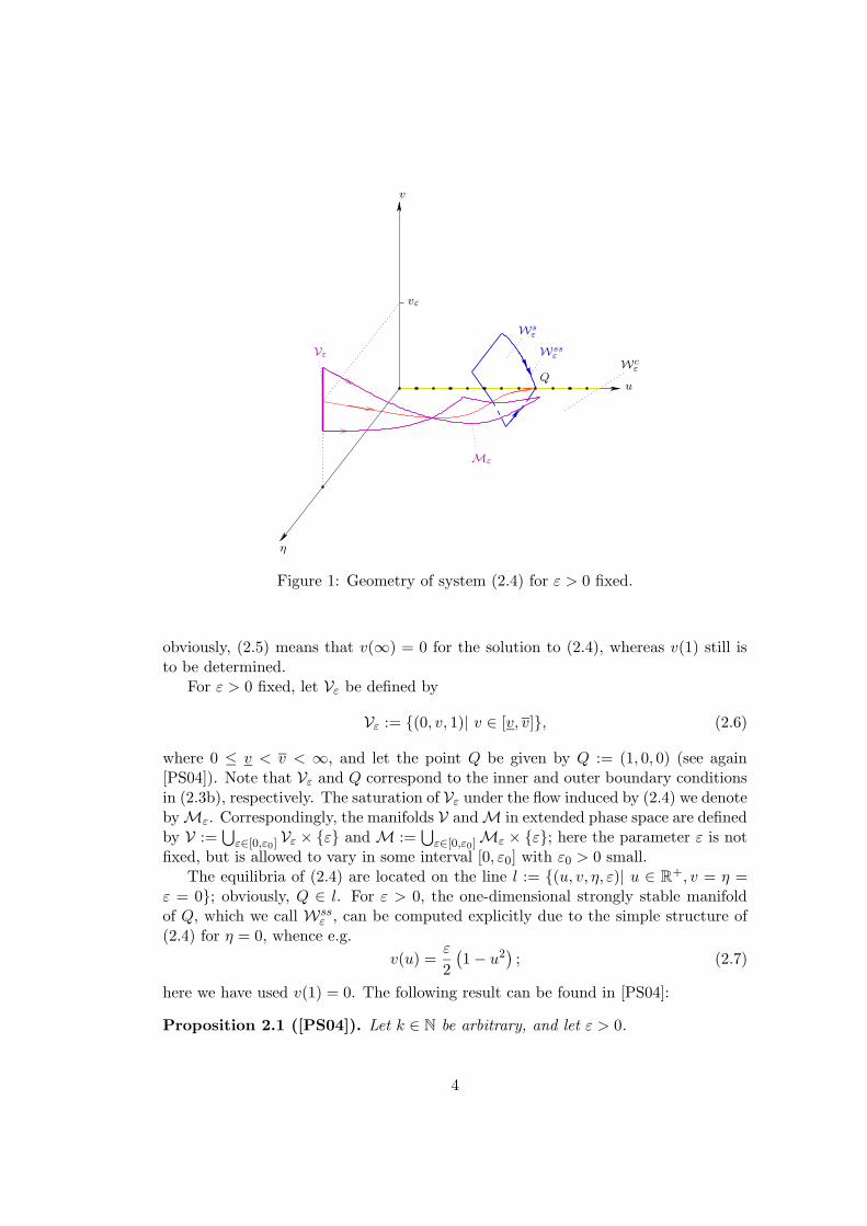
The directional blow-up in the direction of positive η (i.e., in K1) is given by

Φ1 :

{

R4 → R

4

(u1, v1, r1, ε1) 7→ (u1, r1v1, r1, r1ε1),(2.10)

whenceu = u1, v = r1v1, η = r1, ε = r1ε1. (2.11)

After transformation to K1 and desingularization, the equations in (2.4) have thefollowing form:

u′1 = v1

v′1 = (2 − n)v1 − ε1u1v1

r′1 = −r1

ε′1 = ε1.

(2.12)

6

The desingularization, which is necessary to obtain a non-trivial flow for r1 = 0,is performed by dividing out the common factor r1 on both sides of the equations;it corresponds to a rescaling of time, leaving the phase portrait unchanged. Theequilibria of (2.12) are easily seen to lie in l1 := {(u1, v1, r1, ε1)| u1 ∈ R

+, v1 =r1 = ε1 = 0}. A simple computation shows that the corresponding eigenvalues aregiven by −1, 0, and 1 both for n = 3 and for n = 2; these eigenvalues obviouslyare in resonance. In fact, it is these resonances in K1 which are responsible for theoccurrence of logarithmic switchback terms in the Lagerstrom model, as will becomeclear later on.

Similarly, in chart K2, (2.9) is given by

Φ2 :

{

R4 → R

4

(u2, v2, η2, r2) 7→ (u2, r2v2, r2η2, r2)(2.13)

respectivelyu = u2, v = r2v2, η = r2η2, ε = r2, (2.14)

which is simply an ε-dependent rescaling of the original variables, since r2 = ε.Desingularizing once again, we obtain for the blown-up vector field in K2

u′2 = v2

v′2 = (1 − n)η2v2 − u2v2

η′2 = −η22

r′2 = 0;

(2.15)

these equations are simple insofar as r2 occurs only as a parameter. The equilibriaof (2.15) are given by l2 := {(u2, v2, η2, r2)| u2 ∈ R

+, v2 = η2 = 0, r2 ∈ [0, r0]}.The following observation, which is valid in both cases alike, is the starting point

of our analysis:

Proposition 2.2 ([PS04]). Let k ∈ N be arbitrary.

1. There exists an attracting three-dimensional center manifold W c2 of (2.4) which

is given by {v2 = 0}.

2. For |u2−1|, v2, η2, and r2 sufficiently small, there is a stable invariant Ck-smoothfoliation Fs

2 with base Wc2 and one-dimensional Ck-smooth fibers.

Let Wss2 denote the fiber F s

2 (Q2) ∈ Fs2 with base point Q2 := (1, 0, 0, 0); note

that for any r2 = ε ∈ [0, ε0] fixed, Q2 and Wss2 correspond to the original Q and its

stable fiber Wssε , respectively.

Remark 2.1. Just as was the case with Wssε , Wss

2 also is known explicitly: givenv2(1) = 0, one obtains from (2.15) with η2 = 0 that

v2(u2) =1

2

(

1 − u22

)

; (2.16)

hence Wss2 is independent of both ε and n.

7

As in [PS04], let the orbit γ2 be defined by

γ2(ξ2) :={(

1, 0, ξ−12 , 0

)∣

∣ ξ2 ∈ (0,∞)}

, (2.17)

and let Γ2 := γ2 ∪ {Q2}; note that γ2(ξ2) → Q2 as ξ2 → ∞. With Proposition 2.2 itthen follows:

Proposition 2.3 ([PS04]). The manifold Ws2 defined by

Ws2 :=

⋃

P2∈Γ2

F s2 (P2) (2.18)

is an invariant, Ck-smooth manifold, namely the stable manifold of Q2.

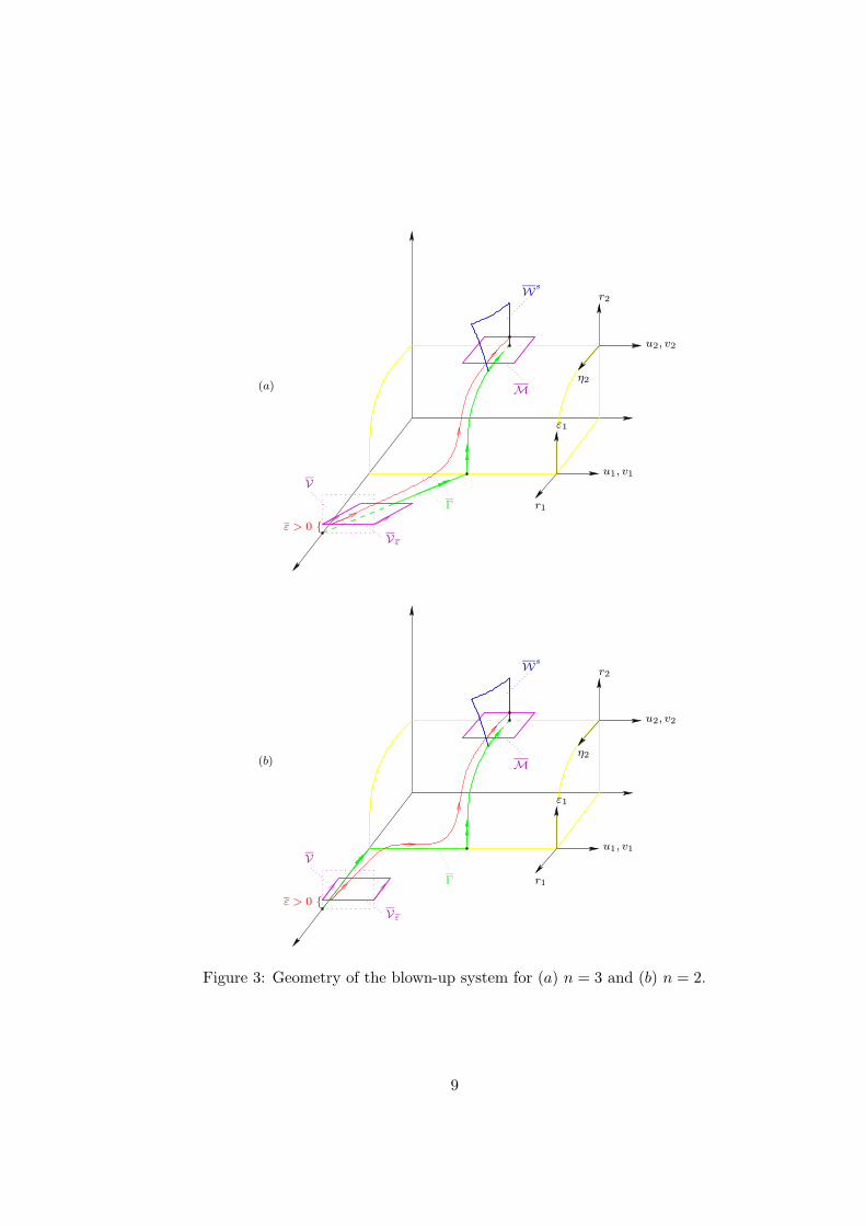
Tracking the manifold Ws2 along the singular orbit Γ to the inner boundary in K1

defines a global manifold Ws

which determines the solution to (2.4),(2.5) as given byTheorem 2.1, see Figure 3.

The relation between charts K1 and K2 on their overlap domain can be describedas follows:

Lemma 2.1 ([PS04]). Let κ12 denote the change of coordinates from K1 to K2, andlet κ21 = κ−1

12 be its inverse. Then κ12 is given by

u2 = u1, v2 = v1ε−11 , η2 = ε−1

1 , r2 = r1ε1 (2.19)

and κ21 is given by

u1 = u2, v1 = v2η−12 , r1 = r2η2, ε1 = η−1

2 . (2.20)

Remark 2.2 (Notation). Let us introduce the following notation: for any object � inthe original setting, let � denote the corresponding object in the blow-up; in chartsKi, i = 1, 2, the same object will appear as �i when necessary.

Moreover, as in [PS04] we define the sections Σin1 , Σout

1 , and Σin2 , where

Σin1 := {(u1, v1, r1, ε1)| u1 ≥ 0, v1 ≥ 0, ε1 ≥ 0, r1 = ρ} (2.21a)

Σout1 := {(u1, v1, r1, ε1)| u1 ≥ 0, v1 ≥ 0, r1 ≥ 0, ε1 = δ} (2.21b)

Σin2 :=

{

(u2, v2, η2, r2)∣

∣ u2 ≥ 0, v2 ≥ 0, r2 ≥ 0, η2 = δ−1}

(2.21c)

with 0 < ρ, δ � 1 arbitrary, but fixed; obviously κ12

(

Σout1

)

= Σin2 .

3 Rigorous asymptotic expansions

We now set out to derive asymptotic expansions for the function v1ε:= v1

∣

∣

ξ=1as

defined by the unique solution to (2.4),(2.5) given in Theorem 2.1, see Figure 4. Itis well-known that to leading order, the method of matched asymptotic expansionsgives

v1ε= 1 − ε ln ε − (γ + 1)ε + O

(

ε2)

(3.1)

8

(a)

(b)

u1, v1

r1

ε1

η2

r2

u2, v2

u1, v1

r1

ε1

η2

r2

u2, v2

ε > 0 {Vε

ε > 0 {Vε

Γ

Γ

Ws

Ws

V

V

M

M

Figure 3: Geometry of the blown-up system for (a) n = 3 and (b) n = 2.

9

ε1

V1 V1

P1P1

(a) (b)

v1εv1ε

r1

v1v1

ε1

r1

Figure 4: v1εfor (a) n = 3 and (b) n = 2.

for n = 3 and

v1ε= −

1

ln ε+

γ

(ln ε)2+ O

(

1

(ln ε)3

)

(3.2)

for n = 2, respectively, see e.g. [Lag88]. Classically, the somewhat surprising oc-currence of logarithmic terms in these expansions has been accounted for under thenotion of switchback; we will show that these terms are in fact due to a resonancephenomenon. Incidentally, note that v1ε

equals dudξ

∣

∣

ξ=1, the analogue of the drag on

the solid, which is a quantity of considerable interest in the original fluid dynamicalproblem.

Our approach is rigorous in the sense that the expansions we compute are approx-imations to a well-defined geometric object, namely, to the invariant manifold W

s

introduced in the previous section. Roughly speaking, our strategy is the following:we begin by computing expansions for Ws

2 in K2; these expansions, when translatedto K1 and evaluated at the inner boundary there, will provide us with expansionsfor v1ε

. We again distinguish between n = 3 and n = 2 here, the case n = 3 beingconsiderably simpler.

Remark 3.1. This strategy, which is slightly different from the strategy applied in[PS04], is somewhat more efficient as far as computing expansions for v1ε

is concerned.Later on we will indicate how asymptotic solution expansions for (2.4),(2.5) can beobtained.

The complicated structure of the expansions in K1 arises as Ws

passes nearthe line of equilibria l1 in K1. As indicated above, the logarithmic terms in (3.1)respectively (3.2) are due to the resonant eigenvalues −1, 0, and 1 which occur inK1, see [PS04]. We now present a simple argument to substantiate our claim: forn = 3, consider the equations in K1 given by (2.12). After introducing the new

10

variable v1 = eξ1v1, one obtains for the first two equations in (2.12)

u′1 = e−ξ1 v1

v′1 = −ε1u1v1.(3.3)

Integration of (3.3) yields1

u1(ξ1) = u10+

∫ ξ1

0e−ξ′ v1(ξ

′) dξ′

v1(ξ1) = v10− ε10

∫ ξ1

0eξ′u1(ξ

′)v1(ξ′) dξ′,

(3.4)

where we have used ε1 = ε10eξ1 and u10

, v10, and ε10

are constants. Note that near l1,v1 and ε1 are small, which implies v1 = O(1) there. Hence a Picard iteration scheme

can be applied to (3.4), with the starting point given by(

u(0)1 , v

(0)1

)

= (u10, v10

).In fact, one easily sees that (3.4) defines a contraction operator for u1 and v1 inL∞[

0, ln ε1

ε10

]

, which ensures convergence of the scheme.2 A straightforward compu-

tation gives

u(1)1 = u10

+ v10

(

1 − e−ξ1)

(3.5a)

v(1)1 = v10

+ ε10u10

v10

(

1 − eξ1)

(3.5b)

u(2)1 = u

(1)1 + ε10

u10v10

(

1 − ξ1 − e−ξ1)

(3.5c)

v(2)1 = v

(1)1 + ε10

v210

(

1 + ξ1 − eξ1)

+1

2ε10

u210

v10

(

1 − 2eξ1 + e2ξ1)

+

+1

2ε10

u10v210

(

3 + 2ξ1 − 4eξ1 + e2ξ1)

(3.5d)

for the first two iterates in (3.4). As ξ1 = ln ε1

ε10

, this then generates a logarithmic

term in ε1 after rewriting (3.5c) as a function of ε1. Similarly, the products of powersof ξ1 and eξ1 which occur for higher iterates in (3.4) will give rise to products ofpowers of ln ε1 and ε1 after those iterates have been rewritten in terms of ε1.

In fact, it is thus possible to obtain successive approximations to the transitionmap Π from Σin

1 to Σout1 for (2.12), see [KS01]; the above computation gives the

leading order behaviour of Π. Note that it is precisely the resonant terms in (2.12)which cannot be eliminated by a normal form transformation and which preclude theexistence of a linearizing transformation for (2.12) proper, see e.g. [CLW94].

1Without loss of generality, we set ξ10= 0 here.

2Incidentally, the introduction of v1 in (2.12) is required for the proof of contractivity of (3.4).

11

3.1 The case n = 3

3.1.1 Expansions in chart K2

As the equations in K2 are completely independent of r2, we can simply omit thelast equation in (2.15), which leaves us with the essentially three-dimensional system

u′2 = v2

v′2 = −2η2v2 − u2v2

η′2 = −η22.

(3.6)

Remark 3.2. In contrast to what is usually done in the literature, we do not intendto derive asymptotic expansions for the solutions to (2.4) here, but rather for themanifold Ws as defined in Section 2. As the solutions to (2.4),(2.5) clearly do dependon ε, however, any ansatz aimed at obtaining solution expansions would of coursehave to take into account this dependence on ε. Note that in our approach, ε entersonly in chart K1, see below.

Given Proposition 2.2, we can make an ansatz for the expansion of W s2 of the

form

v2(u2, η2) =∞∑

j=0

Cj(η2)(u2 − 1)j , (3.7)

where

Cj(η2) :=1

j!

∂j

∂uj2

v2(u2, η2)∣

∣

∣

u2=1, (3.8)

see [vGKS]. Hence

∣

∣

∣

∣

∣

∣

v2(u2, η2) −N∑

j=0

Cj(η2)(u2 − 1)j

∣

∣

∣

∣

∣

∣

= O(

(u2 − 1)N+1)

(3.9)

for any N ∈ N, and the above estimate is uniform for η2 bounded.

Remark 3.3. An equally valid ansatz would be to set

u2(v2, η2) =∞∑

j=0

Dj(η2)vj2, (3.10)

with

Dj(η2) :=1

j!

∂j

∂vj2

u2(v2, η2)∣

∣

∣

v2=0. (3.11)

However, the reason for considering (3.7) and not (3.10) is that ultimately we areinterested in deriving an expansion for v1ε

. Given Lemma 2.1, it is therefore theansatz in (3.7) we have to use.

12

Rewriting (3.6) with η2 as the independent variable and omitting the subscript2, we obtain

du

dη= −

v

η2(3.12a)

dv

dη=

2

ηv +

u − 1

η2v +

v

η2; (3.12b)

inserting (3.7) into (3.12b) yields

∞∑

j=0

[

dCj

dη(u − 1)j − Cjj(u − 1)j−1

(

1

η2

∞∑

k=0

Ck(u − 1)k

)]

=

=2

η

∞∑

j=0

Cj(u − 1)j +1

η2

∞∑

j=0

Cj(u − 1)j+1 +1

η2

∞∑

j=0

Cj(u − 1)j ,

(3.13)

where we have used (3.12a). Collecting powers of u − 1 in (3.13) gives a recursivesequence of differential equations for the coefficient functions in (3.7),

C ′1 −

C1

η

(

C1

η+

1

η+ 2

)

= 0 (3.14a)

C ′j −

Cj

η

(

2 +1

η

)

−j + 1

η2C1Cj =

1

η2Cj−1 +

1

η2

∑

k+l=j+1k,l≥2

kCkCl, j ≥ 2, (3.14b)

with initial conditions

C1(0) = −1, C2(0) = −1

2, Cj(0) = 0, j ≥ 3; (3.15)

note that C0 ≡ 0 due to v(1) = 0. (3.15) is obtained from Remark 2.1, as W ss isgiven by

v(u, 0) = −(u − 1) −1

2(u − 1)2. (3.16)

We will first explicitly solve these equations for j = 1 and afterwards derive thegeneral form of the solution for j arbitrary.

Remark 3.4. Most of the following computations have been performed with the helpof the computer algebra package Maple, see e.g. [Cor02].

From (3.14a) it follows that

C1(η) = −η2

η − eη−1

E1 (η−1) − γ1eη−1, (3.17)

where Ek is in general defined by3

Ek(z) :=

∫ ∞

1e−zττ−k dτ, z ∈ C, <(z) > 0, k ∈ N, (3.18)

3Here <(z) denotes the real part of z.

13

see e.g. [AS64], and γ1 ∈ R is some constant to be determined. With (3.15) and del’Hospital’s rule we obtain limη→0 C1(η) = −1 for γ1 = 0; hence indeed γ1 = 0. Dueto

E2

(

η−1)

= e−η−1

− η−1E1

(

η−1)

(3.19)

we can write

C1(η) = −ηe−η−1

E2 (η−1). (3.20)

As we are interested in (3.7) for η → ∞ (which corresponds to the overlap domain

between the two charts K1 and K2), we expand E2

(

η−1)−1

about η = ∞ to obtainan indication as to what the Cjs might look like in general:

E2

(

η−1)−1

= 1 + (1 − γ)η−1 + η−1 ln η +

(

γ2 − 2γ +3

2

)

η−2+

+ 2γη−2 ln η + η−2(ln η)2 + O(

η−3)

,

(3.21)

which implies

C1(η) = ηe−η−1

∞∑

k,l=0

γ1klη

−k(ln η)l. (3.22)

We will show that Cj can in fact be expanded as in (3.22) for any j ∈ N. To thatend, note that e.g. for j = 2, equation (3.14b) becomes

C ′2 −

C2

η

(

2 +1

η

)

+3e−η−1

ηE2 (η−1)C2 = −

e−η−1

ηE2 (η−1), (3.23)

which has the solution

C2(η) =

(

−

∫

e3

∫

e−η′−1

η′−1E2

(

η′−1)−1

dη′

η−3E2

(

η−1)−1

dη + γ2

)

×

×η2e−η−1

e−3

∫

e−η−1

η−1E2

(

η−1)−1

dη;

(3.24)

here we have used (3.20). (3.24) obviously cannot be integrated in closed form. Still,one can derive the following result concerning the structure not only of C2, but ofany Cj with j ≥ 2:

Proposition 3.1. For j ≥ 1, the solution Cj(η) to (3.14),(3.15) can be written as

Cj(η) = ηe−η−1

∞∑

k,l=0

γjklη

−k(ln η)l. (3.25)

Here γjkl ∈ R are constants to be determined from (3.15).

14

Proof. The proof is by an induction argument: for i = 1, the assertion is obviouslyvalid, see (3.22); let us assume that it holds for i = 1, . . . , j−1. For the homogeneoussolution to (3.14b) one finds

Chomj (η) = γjη

2e−η−1

e−(j + 1)

∫

e−η−1

η−1E2

(

η−1)−1

dη; (3.26)

the integrand in (3.26) can be expanded as

−e−η−1

ηE2 (η−1)= −η−1 + γη−2 − η−2 ln η + O

(

η−3)

, (3.27)

whence

e(j + 1)

∫

[

−η−1 + γη−2 − η−2 ln η + O(

η−3)]

dη= O

(

η−j−1)

, j ≥ 2. (3.28)

For (3.26) the claim now follows from (3.21), (3.28), and the following lemma:

Lemma 3.1. For any α, β ∈ Z,

∫

zα(ln z)β dz =

zα+1(ln z)β

α + 1−

β

α + 1

∫

zα(ln z)β−1 dz, α 6= −1

(ln z)β+1

β + 1, α = −1.

(3.29)

For the particular solution, note first that by the induction hypothesis, the right-hand side of (3.14b) can be written as

1

η2Cj−1 +

1

η2

∑

k+l=j+1k,l≥2

kCkCl = e−η−1

∞∑

m,n=0

γjmnη−m(ln η)n. (3.30)

A particular solution to

C ′j −

Cj

η

(

2 +1

η

)

+ (j + 1)e−η−1

ηE2 (η−1)Cj = e−η−1

η−m(ln η)n (3.31)

is given by

Cpartj (η) =

∫

η−m−2(ln η)ne(j + 1)

∫

e−η′−1

η′−1E2

(

η′−1)−1

dη′

dη×

× η2e−η−1

e−(j + 1)

∫

e−η−1

η−1E2

(

η−1)−1

dη;

(3.32)

With (3.21), (3.28), and Lemma 3.1, this concludes the proof, as m, n ≥ 0 andj ≥ 2.

15

We can even obtain a somewhat more precise result on the structure of Cj , j ≥ 1.Let (k, l) denote the index of a term η−k(ln η)l in (3.25); given this notation, we havethe following

Proposition 3.2. A term with index (k, l) can occur in (3.25) only if l ≤ k.

Proof. The proof is again by induction: for i = 1, the assertion is obvious from (3.20)and (3.21). Given the assertion for i = 1, . . . j − 1, it follows immediately from (3.28)and Lemma 3.1 that it holds for the homogeneous part (3.26) of Cj , as well. To provethe assertion for (3.32), we proceed as follows: as in [vGKS] we define a map, say,ι(m, n), which assigns to the index of a term in (3.30) the set of indices of the termsit generates in (3.32). By (3.28) and the proof of Proposition 3.1 one then easily seesthat with Lemma 3.1,

ι(m, n) =

{

{(m + m′, n + n′), (m + m′, n + n′ − 1), . . . , (m + m′, 0)}, m 6= j

{(j + m′ + 1, n + n′ + 1)}, m = j;

(3.33)here m′, n′ ∈ N with n′ ≤ m′. This completes the proof, as n ≤ m by assumption.

3.1.2 Expansions in chart K1

Given Proposition 3.1, we are able to derive asymptotic expansions for W s2 in K2 for

η2 → ∞. To get the desired expansion for v1ε, however, we need to know what these

expansions correspond to in K1. First, note that with Lemma 2.1, (3.7) becomes

ε−11 v1(u1, ε1) =

∞∑

j=0

Aj(ε1)(u1 − 1)j , (3.34)

where

Aj(ε1) =e−ε1

ε1

∞∑

k,l=0l≤k

αjklε

k1(ln ε1)

l; (3.35)

here αjkl = (−1)lγ

jkl. It remains to show that (3.35) does indeed make sense for ε1 → 0

(which is equivalent to η2 → ∞ in K2). To that end, we assume that a curve of initialconditions in Σout

1 of the form

(u1, v1, ε1) =(

uout1 , vout

1

(

uout1

)

, δ)

, vout1 (1) = 0 (3.36)

is given, and we investigate the corresponding invariant manifold consisting of seg-ments of solutions of (2.12). By variation of constants integrating backwards from

16

Σout1 , this manifold can be represented as follows:

u1

(

ξ1, uout1

)

= uout1 −

∫ Ξ

ξ1

v1

(

ξ′, uout1

)

dξ′ (3.37a)

v1

(

ξ1, uout1

)

=δ

εvout1

(

uout1

)

e−ξ1 + e−ξ1

∫ Ξ

ξ1

eξ′ε1(ξ′)u1

(

ξ′, uout1

)

v1

(

ξ′, uout1

)

dξ′

(3.37b)

ε1(ξ1) = εeξ1 , (3.37c)

where Ξ = ln δε. We have the following result:

Proposition 3.3. Let vout1

(

uout1

)

be Ck-smooth for some k ∈ N. Then, for j =

0, . . . , k, ∂j

∂uj1

v1(u1, ε1) exists and is continuous for ε1 ∈ [0, δ] and |u1 − 1| ≤ β with

β > 0 sufficiently small.

Proof. Changing the integration variable to ε1 in (3.37), we obtain

u1(ε1) = uout1 −

∫ δ

ε1

v1(u1(ε′), ε′)

dε′

ε′(3.38a)

v1(u1, ε1) =δ

ε1vout1 +

1

ε1

∫ δ

ε1

ε′u1(ε′)v1(u1(ε

′), ε′) dε′; (3.38b)

here ε′ = εeξ′ . Then (3.38) together with

u1(ε′) ∼ uout

1 + vout1

(

1 −δ

ε′

)

, v1(u1(ε′), ε′) ∼

δ

ε′vout1 (3.39)

implies that v1 remains continuous in (u1, ε1) for ε1 → 0. Differentiating (3.38)formally with respect to u1 yields

1 =duout

1

du1−

∫ δ

ε1

∂v1(u1(ε′), ε′)

∂u1dε′ (3.40a)

∂v1(u1, ε1)

∂u1=

δ

ε1

dvout1

du1+

1

ε1

∫ δ

ε1

ε′[

du1(ε′)

du1v1(u1(ε

′), ε′) + u1(ε′)

∂v1(u1(ε′), ε′)

∂u1

]

dε′;

(3.40b)

as we have dε′

dε1= ε′

ε1, it follows that

du1(ε′)

du1=

v1(u1(ε′), ε′)

v1(u1(ε1), ε1), (3.41)

whence∂v1(u1(ε

′), ε′)

∂u1=

∂v1(u1(ε′), ε′)

∂u1(ε′)

v1(u1(ε′), ε′)

v1(u1(ε1), ε1). (3.42)

17

Q1

v1ε= v1(0, ε) =

∞∑

i,j=0

j≤i

aij(0)εi(ln ε)j

v1(u1, ε1) =

∞∑

i,j=0

j≤i

aij(u1)εi1(ln ε1)j

ε−1

1v1(u1, ε1) =

∞∑

j=0

Aj(ε1)(u1 − 1)j

ε1

Γ1

P out1

u1

v1

P in1

P1

Σout1

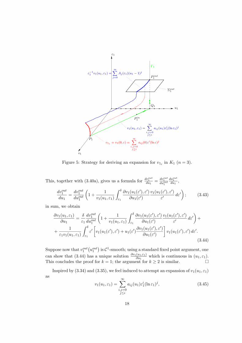
Figure 5: Strategy for deriving an expansion for v1εin K1 (n = 3).

This, together with (3.40a), gives us a formula fordvout

1

du1=

dvout1

duout1

duout1

du1,

dvout1

du1=

dvout1

duout1

(

1 +1

v1(u1, ε1)

∫ δ

ε1

∂v1(u1(ε′), ε′)

∂u1(ε′)

v1(u1(ε′), ε′)

ε′dε′)

; (3.43)

in sum, we obtain

∂v1(u1, ε1)

∂u1=

δ

ε1

dvout1

duout1

(

1 +1

v1(u1, ε1)

∫ δ

ε1

∂v1(u1(ε′), ε′)

∂u1(ε′)

v1(u1(ε′), ε′)

ε′dε′)

+

+1

ε1v1(u1, ε1)

∫ δ

ε1

ε′[

v1(u1(ε′), ε′) + u1(ε

′)∂v1(u1(ε

′), ε′)

∂u1(ε′)

]

v1(u1(ε′), ε′) dε′.

(3.44)

Suppose now that vout1

(

uout1

)

is C1-smooth; using a standard fixed point argument, one

can show that (3.44) has a unique solution ∂v1(u1,ε1)∂u1

which is continuous in (u1, ε1).This concludes the proof for k = 1; the argument for k ≥ 2 is similar.

Inspired by (3.34) and (3.35), we feel induced to attempt an expansion of v1(u1, ε1)as

v1(u1, ε1) =∞∑

i,j=0j≤i

aij(u1)εi1(ln ε1)

j , (3.45)

18

see Figure 5; the requirement that j ≤ i in the summation in (3.45) is a consequenceof Proposition 3.2. The coefficient functions aij , 0 ≤ j ≤ i, will be determineduniquely by the demand for smoothness in u1 and by the requirement that, seen asa double expansion, (3.45) should agree with (3.34). To that end, let us introduce u1

as the independent variable in (2.12), whence4

dv

du= −1 − εu

dε

du=

ε

v.

(3.46)

Remark 3.5. With (3.10) instead of (3.7) in K2, we would now have

u(v, ε) =∞∑

i,j=0j≤i

bij(v)εi(ln ε)j (3.47)

instead of (3.45). One can easily check that the following considerations would thengo through just the same, with only a few minor adjustments required.

By proceeding just as in K2 and multiplying the resulting equations with v, weobtain

∞∑

i,j=0j≤i

a′ijεi(ln ε)j

∞∑

k,l=0l≤k

aklεk(ln ε)l

+ aijεi(ln ε)j−1(i ln ε + j)

=

= (−1 − εu)

∞∑

i,j=0j≤i

aijεi(ln ε)j ,

(3.48)

where ′ = ddu

now. We do not bother to look for the general solution to (3.48) rightnow, but will for the moment only consider the first few terms in (3.45); hence e.g.for 0 ≤ j ≤ i ≤ 2,

a′00a00 = −a00 (3.49a)

a′11a00 + a′00a11 + a11 = −a11 (3.49b)

a′10a00 + a′00a10 + a10 + a11 = −a10 − ua00 (3.49c)

a′22a00 + a′11a11 + a′00a22 + 2a22 = −a22 (3.49d)

a′21a00 + a′11a10 + a′10a11 + a′00a21 + 2a21 + 2a22 = −a21 − ua11 (3.49e)

a′20a00 + a′10a10 + a′00a20 + 2a20 + a21 = −a20 − ua10. (3.49f)

Note that these equations can be solved recursively: (3.49a) yields either a00 ≡ 0 ora′00 = −1; however, for (3.34) and (3.45) to agree when seen as double expansions,we have to take the latter, see (3.20), whence

a00 = −u + α00. (3.50)

19

ε1

P in1

P out1

Σout1

Σin1

v1

Γ1

u1

Q1

Figure 6: Overlap domain (shaded) of expansions (3.34) and (3.45).

Here α00 is a constant which is to be determined from (3.34); indeed, it followsfrom (3.20) and (3.21) that an expansion for v is given by

v(u, ε) =[

−1 + γε + ε ln ε + O(

ε2)]

(u − 1) + O(

(u − 1)2)

. (3.51)

To obtain agreement to lowest order between (3.34) and (3.45), we hence have totake α00 = 1.

By plugging (3.50) into (3.49b) and solving the resulting equation

−a′11(u − 1) + a11 = 0, (3.52)

one then hasa11 = α11(u − 1). (3.53)

Similarly, (3.50) and (3.53) together with (3.49c) give

−a′10(u − 1) + a10 = (u − α11)(u − 1), (3.54)

which has the solution

a10 = −(u − 1)2 − (1 − α10)(u − 1) − (1 − α11)(u − 1) ln (u − 1); (3.55)

for (3.55) to be smooth, α11 has to be chosen such that the ln (u − 1)-terms in (3.56)vanish, which implies α11 = 1. The requirement that (3.34) and (3.45) should agreethen gives α10 = 1 + γ, see (3.51):

a10 = −(u − 1)2 + γ(u − 1). (3.56)

4Again the subscript 1 will be omitted.

20

For (3.49d), (3.49e), and (3.49f), one obtains by the same procedure

a22 = (u − 1)2 − (u − 1) (3.57a)

a21 = (2γ + 1)(u − 1)2 − (2γ − 1)(u − 1) (3.57b)

a20 = (u − 1)3 + (1 + α20)(u − 1)2 − (γ2 − γ + 1)(u − 1), (3.57c)

where α22 = 1 and α21 = 2γ + 1 have again been chosen such that the ln (u − 1)-terms in (3.57b) and (3.57c) cancel and α20 has to be determined by comparing theleading-order terms in (3.34) and (3.45).

Remark 3.6. The above procedure is in fact closely related to the approach one wouldclassically take when matching (3.34) and (3.45). As these two expansions have toagree on the overlap domain between the two charts K1 and K2, it is there onewould have to define an intermediate variable. Note that in [HTB90], say, logarith-mic switchback is handled using a modified version of the block matching principleintroduced by [vD75]: terms are matched in blocks according to the powers of ε

they contain, with no distinction being made for any additional logarithmic factors.Our approach seems to justify this principle, as the logarithmic factors in (3.45) aredetermined simply by the requirement that aij be smooth.

One expects, of course, that the above procedure can be carried out to any order ini and j in (3.48), where for i fixed one starts with j = i and then proceeds recursivelydown to j = 0. That this is indeed possible is contained in the following result:

Proposition 3.4. There exist unique smooth functions aij(u1) such that (3.34) and(3.45), seen as double expansions, are the same.

Proof. We proceed just as in computing the first few coefficients of (3.45) above: forfixed i we successively solve (3.48), starting with j = i. By induction we will establish

aij =i∑

k=1

αijk (u − 1)k, 1 ≤ j ≤ i, (3.58a)

ai0 =i+1∑

k=1

αi0k (u − 1)k, j = 0 (3.58b)

for any i ≥ 1 and 0 ≤ j ≤ i, with some constants αijk ∈ R to be chosen appropriately.

Indeed, for i = 1 the claim follows from (3.53) and (3.56) by inspection. Let usassume that (3.58) is valid for akl, where k = 1, . . . , i − 1 and l ≤ k. By plugging(3.50) into (3.48) and collecting powers of ε ln ε, one obtains

−a′ij(u − 1) + iaij = −(j + 1)ai,j+1 − uai−1,j −∑

k+m=il+n=j

l≤k≤i−1, n≤m≤i−1

a′klamn; (3.59)

21

here we have used a′00 = −1. The homogeneous solution to (3.59) is given by

αij(u − 1)i, 0 ≤ j ≤ i (3.60)

with some constant αij ; to complete the proof, we have to consider the followingcases:

• for j = i, equation (3.59) becomes

−a′ii(u − 1) + iaii = −∑

k+m=ik,m≥1

a′kkamm, (3.61)

which has the solution

aii = αii(u − 1)i +i−1∑

k=1

αiik (u − 1)k, (3.62)

as by (3.58)

−∑

k+m=ik,m≥1

a′kkamm = −

i−1∑

k=1

αiik (u − 1)k (3.63)

and a term −αiik (u − 1)k gives a particular solution of the form

−αii

k

i − k(u − 1)k, 1 ≤ k ≤ i − 1; (3.64)

the constant αii remains to be determined in one of the next steps.

• for j = i − 1 (which is indeed representative of all further cases), one obtains

−a′i,i−1(u − 1) + iai,i−1 = −iaii − uai−1,i−1−

−∑

k+m=ik,m≥1

[

a′kkam,m−1 + akka′m,m−1

]

, (3.65)

where the homogeneous solution is again given by (3.60). As for the inhomo-geneity, note that terms of the form −iαii

k (u − 1)k in −iaii generate particularsolutions of the form

iαii(u − 1)i ln (u − 1), k = i, (3.66a)

−iαii

k

i − k(u − 1)k, 1 ≤ k ≤ i − 1. (3.66b)

Similarly, for the terms −αi−1,i−1k u(u − 1)k in −uai−1,i−1 one obtains

αi−1,i−1i−1 (u − 1)i−1((u − 1) ln (u − 1) − 1), k = i − 1, (3.67a)

−α

i−1,i−1i−2

(i − k)(i − k − 1)(u − 1)k(−1 + (i − k)u), 1 ≤ k ≤ i − 2. (3.67b)

22

By the induction hypothesis, for the remaining terms one has

−∑

k+m=ik,m≥1

[

a′kkam,m−1 + akka′m,m−1

]

= −i∑

k=0

αi,i−1k (u − 1)k (3.68)

for some constants αi,i−1k ∈ R. Just as above, the terms −α

i,i−1k (u − 1)k give

rise to terms of the form

αi,i−1i (u − 1)i ln (u − 1), k = i, (3.69a)

−α

i,i−1k

i − k(u − 1)k, 1 ≤ k ≤ i − 1. (3.69b)

In sum, one thus has

ai,i−1 = αi,i−1(u − 1)i +i−1∑

k=1

αi,i−1k (u − 1)k+

+(

iαii + αi−1,i−1i−1 + α

i,i−1i

)

ln (u − 1)(u − 1)i,

(3.70)

where αii is now chosen such that (3.70) is smooth, i.e., such that the ln (u − 1)-terms cancel, and αi,i−1 still is at our disposal.

• for 1 ≤ j ≤ i − 2 in general, one repeats the same procedure, i.e., one solves(3.59) and subsequently fixes αi,j+1 appropriately so as to eliminate any ln (u − 1)-terms in aij , guaranteeing the smoothness of aij .

• in the final step, for j = 0, additional terms of O(

(u − 1)i+1)

are generated as

claimed due to the terms −αi−1,0i u(u−1)i and −αi0

i (u−1)i+1 in the right-handside of (3.59) giving

αi−1,0i (u + ln (u − 1)) (u − 1)i (3.71)

andαi0

i u(u − 1)i (3.72)

in ai0, respectively. One is then left with αi1 and αi0, which one chooses suchas to make sure that ai0 is smooth and that (3.34) and (3.45) agree if both areseen as double expansions, which concludes the proof.

We are now ready to formulate the main result of this section, namely, to give anexpansion of v1ε

for n = 3:

Proposition 3.5. For ε ∈ (0, ε0] with ε0 > 0 sufficiently small, v1ε= v1(0, ε) can be

expanded as

v1ε= 1 − ε ln ε − (γ + 1)ε + 2ε2(ln ε)2 + 4γε2 ln ε + O

(

ε3)

. (3.73)

23

Proof. By plugging (3.50), (3.53), (3.56), (3.57a), and (3.57b) into (3.45), one obtainsthe following expansion for v1:

v1(u1, ε1) = −(u1 − 1) + (u1 − 1)ε1 ln ε1 +[

−(u1 − 1)2 + γ(u1 − 1)]

ε1+

+[

(u1 − 1)2 − (u1 − 1)]

ε21(ln ε1)

2+

+[

(2γ + 1)(u1 − 1)2 − (2γ − 1)(u1 − 1)]

ε21 ln ε1 + O

(

ε31

)

.

(3.74)

The assertion now follows with u1 = 0 and ε1 = ε in (3.74).

Remark 3.7. Note that the expansion in (3.73) is equally valid in the original settingof (2.4), i.e., vε = v1ε

, as is easily seen by performing the appropriate blow-downtransformation, which is trivial here. Analogous results have been obtained in theliterature, see e.g. [Lag88].

3.2 The case n = 2

Although the case n = 2 is potentially more difficult, we can use the same strategyas before to compute expansions for v1ε

. Not surprisingly, however, computationallythe analysis is more involved now, due to the extensive switchback which arises inthe matching process for n = 2.

3.2.1 Expansions in chart K2

As the situation in K2 is very similar to that for n = 3, we will not go into too manydetails: given the ansatz

v2(u2, η2) =∞∑

j=0

Cj(η2)(u2 − 1)j , (3.75)

which we plug into (3.6) rewritten with η2 as the independent variable,

du

dη= −

v

η2(3.76a)

dv

dη=

v

η+

u − 1

η2v +

v

η2, (3.76b)

we obtain a recursive sequence of equations for Cj , j ≥ 1, by comparing powers ofu − 1:

C ′1 −

C1

η

(

C1

η+

1

η+ 1

)

= 0 (3.77a)

C ′j −

Cj

η

(

1 +1

η

)

−j + 1

η2C1Cj =

1

η2Cj−1 +

1

η2

∑

k+l=j+1k,l≥2

kCkCl, j ≥ 2. (3.77b)

24

The initial conditions are again given by

C1(0) = −1, C2(0) = −1

2, Cj(0) = 0, j ≥ 3; (3.78)

moreover, C0 ≡ 0 just as for n = 3. From (3.77a) we have

C1(η) = −ηe−η−1

E1 (η−1) + γ1

; (3.79)

as limη→0 C1(η) = −1 for γ1 = 0, we conclude that γ1 = 0 again. The expansion of

E1

(

η−1)−1

about η = ∞ is given by

E1

(

η−1)−1

= (ln η − γ)−1 − η−1(ln η − γ)−2 +1

4η−2(ln η − γ)−2+

+ η−2(ln η − γ)−3 + O(

η−3)

,

(3.80)

whence

C1(η) = ηe−η−1

∞∑

k,l=0

γ1klη

−k(ln η − γ)−l; (3.81)

here γ is Euler’s constant, as before. For j = 2, (3.77b) gives

C ′2 −

C2

η

(

1 +1

η

)

+3e−η−1

ηE1 (η−1)C2 = −

e−η−1

ηE1 (η−1), (3.82)

which has the solution

C2(η) =

(

−

∫

η−2E1

(

η−1)2

dη + γ2

)

ηe−η−1

E1

(

η−1)−3

. (3.83)

Although (3.83) cannot be integrated in closed form, we still have the following result,which is similar to the one derived for n = 3:

Proposition 3.6. For j ≥ 1, the solution Cj(η) to (3.77),(3.78) can be written as

Cj(η) = ηe−η−1

∞∑

k,l=0

γjklη

−k(ln η − γ)−l. (3.84)

Here γjkl ∈ R are constants to be determined from (3.15).

Proof. The proof is very similar to that of Proposition 3.1: for i = 1, the assertionholds by (3.79); let it be valid for i = 1, . . . , j − 1. The homogeneous solution to(3.77b) is given by

Chomj (η) = γj

ηe−η−1

E1 (η−1)j+1, (3.85)

25

where E1

(

η−1)−j−1

can be expanded as

E1

(

η−1)−j−1

= (ln η − γ)−j−1 − (j + 1)η−1(ln η − γ)−j−2+

+1

4(j + 1)η−2(ln η − γ)−j−2 +

1

2(j + 1)(j + 2)η−2(ln η − γ)−j−3 + O

(

η−3)

.

(3.86)

Given the induction hypothesis, the right-hand side of (3.77b) has the following form:

1

η2Cj−1 +

1

η2

∑

k+l=j+1k,l≥1

kCkCl = e−η−1

∞∑

m,n=0

γjmnη−m(ln η − γ)−n; (3.87)

a particular solution of (3.77b) corresponding to a term e−η−1

η−m(ln η−γ)−n is givenby

Cpartj (η) =

∫

η−m−1(ln η − γ)−nE1

(

η−1)j+1

dη · ηe−η−1

E1

(

η−1)−j−1

. (3.88)

With the substitution η′ = ηγ

and (3.86), the integrand in (3.88) can be written as

∞∑

m′=m+1n′=n−j−1

γmnm′n′η′−m′

(ln η′)−n′

; (3.89)

the claim now follows from Lemma 3.1 with η′ again replaced by η.

Note, however, that we can state no analogue to Proposition 3.2 here; in fact, itseems that any index pair (k, l) can occur in (3.45) now.

3.2.2 Expansions in chart K1

As in the case n = 3, in order to obtain an expansion for v1ε, it now remains to

translate (3.7) to K1. Lemma 2.1 again gives

ε−11 v1(u1, ε1) =

∞∑

j=0

Aj(ε1)(u1 − 1)j , (3.90)

see (3.34), where

Aj(ε1) =e−ε1

ε1

∞∑

k,l=0

αjkl

εk1

(ln ε1 + γ)l(3.91)

with αjkl = (−1)lγ

jkl.

26

Remark 3.8 (Transcendentally small terms). Terms in powers of ε1, as well as termsin powers of ε1 multiplied by powers of (ln ε1 + γ)−1, are smaller than all positivepowers of (ln ε1 + γ)−1: they are said to be beyond all orders of (ln ε1 + γ)−1, orto be transcendentally small terms. In the original setting of flow around a circularcylinder, [Ski75] showed how to calculate a few of these terms. He pointed out,however, that they are in fact negligible: it is the only very slight asymmetry in theflow field which indicates the relative insignificance of these inertial terms for lowReynolds numbers, see [Ski75] for a detailed analysis.

As for n = 3, using variation of constants we can again write

u1

(

ξ1, uout1

)

= uout1 −

∫ Ξ

ξ1

v1

(

ξ′, uout1

)

dξ′ (3.92a)

v1

(

ξ1, uout1

)

= vout1

(

uout1

)

+

∫ Ξ

ξ1

ε1(ξ′)u1

(

ξ′, uout1

)

v1

(

ξ′, uout1

)

dξ′ (3.92b)

ε1(ξ1) = εeξ1 (3.92c)

for the manifold consisting of segments of solutions to (2.12) given the initial curve(3.36). In analogy to Proposition 3.3 we now have

Proposition 3.7. Let vout1

(

uout1

)

be Ck-smooth for some k ∈ N. Then, for j =

0, . . . , k, ∂j

∂uj1

v1(u1, ε1) exists and is continuous for ε1 ∈ [0, δ] and |u1 − 1| ≤ β with

β > 0 sufficiently small.

Proof. The proof is the same as for n = 3, with the relevant relations given by

u1(ε1) = uout1 −

∫ δ

ε1

v1(u1(ε′), ε′)

dε′

ε′(3.93a)

v1(u1, ε1) =δ

ε1vout1 +

1

ε1

∫ δ

ε1

u1(ε′)v1(u1(ε

′), ε′) dε′ (3.93b)

and

∂v1(u1, ε1)

∂u1=

dvout1

duout1

(

1 +1

v1(u1, ε1)

∫ δ

ε1

∂v1(u1(ε′), ε′)

∂u1(ε′)

v1(u1(ε′), ε′)

ε′dε′)

+

+1

v1(u1, ε1)

∫ δ

ε1

[

v1(u1(ε′), ε′) + u1(ε

′)∂v1(u1(ε

′), ε′)

∂u1(ε′)

]

v1(u1(ε′), ε′) dε′

(3.94)

now, respectively.

To derive an expansion for v1(u1, ε1) of the form

v1(u1, ε1) =∞∑

i,j=0

aij(u1)εi1

(ln ε1 + γ)j, (3.95)

27

P1

P out1

Γ1

P in1

Q1

v1(u1, ε1) =

∞∑

i,j=0

aij(u1)εi1

(ln ε1 + γ)j

v1ε= v1(0, ε) =

∞∑

i,j=0

aij(0)εi

(ln ε + γ)j

ε−1

1v1(u1, ε1) =

∞∑

j=0

Aj(ε1)(u1 − 1)j

ε1

v1

u1

Σout1

Figure 7: Strategy for deriving an expansion for v1εin K1 (n = 2).

we have to consider

dv

du= −εu

dε

du=

ε

v,

(3.96)

which yields

∞∑

i,j=0

a′ijεi

(ln ε + γ)j

∞∑

k,l=0

aklεk

(ln ε + γ)l

+ aijεi

(ln ε + γ)j

(

i −j

ln ε + γ

)

=

= −εu

∞∑

i,j=0

aijεi

(ln ε + γ)j.

(3.97)

Collecting powers of ε(ln ε + γ)−1 in (3.97), we obtain the following sequence of

28

equations for aij with 0 ≤ i + j ≤ 3:

a′00a00 = 0 (3.98a)

a′01a00 + a′00a01 = 0 (3.98b)

a′10a00 + a′00a10 + a10 = −ua00 (3.98c)

a′02a00 + a′00a02 + a′01a01 − a01 = 0 (3.98d)

a′11a00 + a′00a11 + a′10a01 + a′01a10 + a11 = −ua01 (3.98e)

a′20a00 + a′00a20 + a′10a10 + 2a20 = −ua10 (3.98f)

a′03a00 + a′00a03 + a′02a01 + a′01a02 − 2a02 = 0 (3.98g)

a′12a00 + a′00a12 + a′11a01 + a′01a11 + a′10a02 + a′02a10 + a12 − a11 = −ua02 (3.98h)

a′21a00 + a′00a21 + a′20a01 + a′01a20 + a′11a10 + a′10a11 + 2a21 = −ua11 (3.98i)

a′30a00 + a′00a30 + a′20a10 + a′10a20 + 3a30 = −ua20. (3.98j)

Here we have proceeded by diagonalization: as we do not have such precise infor-mation on the structure of (3.84) as we had for n = 3, a simple recursion will notwork. We thus have to take a different approach, comparing coefficients in (3.97) fori + j = p constant.

Let us illustrate the procedure by explicitly solving the first few equations in(3.98): from (3.98a) we have a00 ≡ 0 or a′00 = 0; however, for (3.90) and (3.95) toagree, we have to take the former, which substantially simplifies all further arguments.Equation (3.98b) is vacuous, as indeed 0 = 0, whereas (3.98c) then immediatelyyields a10 ≡ 0. Given a00 ≡ 0, (3.98d) implies either a01 ≡ 0 or a′01 = 1. Here therequirement that (3.90) and (3.95) agree to lowest order fixes a′

01 = 1, whence

a01 = u + α01 (3.99)

for some α01 ∈ R. In fact, with (3.79) and (3.80) one finds

v(u, ε) =

[

1

ln ε + γ−

ε

ln ε + γ+

ε

(ln ε + γ)2+

1

2

ε2

ln ε + γ−

5

4

ε2

(ln ε + γ)2+

+ε2

(ln ε + γ)3+ O

(

ε3)

]

(u − 1) + O(

(u − 1)2)

,

(3.100)

which implies α01 = −1. Plugging (3.99) into (3.98e) then gives

a11 = −(u − 1)2 − (u − 1); (3.101)

moreover, it follows from (3.98f) that a20 ≡ 0, as well. Again with (3.99), equation(3.98g) becomes

a′02(u − 1) − a02 = 0, (3.102)

which has the solutiona02 = α02(u − 1) (3.103)

29

for some constant α02. With reference to (3.100) one can fix α02, whence α02 = 0.As for a12 and a21, one easily obtains from (3.98h) and (3.98i) that

a12 = 2(u − 1)2 + u − 1 (3.104)

and

a21 =1

2(u − 1)3 + (u − 1)2 +

1

2(u − 1), (3.105)

respectively, whereas a30 ≡ 0. As for n = 3, we can now prove the following generalresult:

Proposition 3.8. There exist unique smooth functions aij(u1) such that (3.90) and(3.95), seen as double expansions, are the same.

Proof. The proof differs significantly from the one we gave for n = 3, although it isagain by induction, now on the sum i + j instead of on i alone, however. We willshow

aij =

i+j∑

k=1

αijk (u − 1)k, i, j ≥ 1, (3.106a)

a0j =

j−1∑

k=1

α0jk (u − 1)k, j ≥ 2, (3.106b)

ai0 ≡ 0, i ≥ 2; (3.106c)

indeed, for i + j = 2, the assertion is obvious from (3.101) and (3.103). Let (3.106)be valid for i+ j = 2, . . . , p− 1; we have to show that it is valid for i+ j = p, as well.Collecting powers of ε(ln ε + γ)−1 in (3.97), we obtain

∑

k+m=il+n=j

[

a′klamn + a′mnakl

]

+ iaij − (j − 1)ai,j−1 = −uai−1,j . (3.107)

Plugging a00 ≡ 0 and (3.99) into (3.107) gives the following equation for a0p:

a′0p(u − 1) − (p − 1)a0p = −∑

k+l=p+1k,l≥2

[a′0ka0l + a′0la0k]; (3.108)

by the induction hypothesis, the above sum can be written as

−

p−2∑

k=1

α0pk (u − 1)k. (3.109)

As terms of the form −α0pk (u − 1)k generate particular solutions of the form

−α

0pk

k − p + 1(u − 1)k, 1 ≤ k ≤ p − 2 (3.110)

30

in (3.108) and the homogeneous solution is given by

α0p(u − 1)p−1, (3.111)

for a0p the claim follows. Note that the constant α0p has to be chosen such that (3.90)and (3.95) agree when seen as double expansions; the smoothness of a0p is grantedirrespective of the choice of α0p. For aij with i + j = p and i ≥ 1, (3.107) yields

iaij = jai,j−1 − uai−1,j −∑

k+m=il+n=j

[a′klamn + a′mnakl]; (3.112)

due to the fact that a00 ≡ 0, this completely determines aij . Moreover, it follows fromthe induction hypothesis that aij is of the desired form and that ap0 ≡ 0, respectively,which concludes the proof.

Remark 3.9. The above proof shows that once the leading-order behaviour in (3.95)is determined, the transcendentally small terms in (3.95) are given as solutions notof differential, but of algebraic equations. Our approach thus immediately providesus with these terms, whereas in the classical approach, quite cumbersome computa-tions are required for their determination, as matching is typically done only up totranscendentally small quantities there.

We can now give an expansion of v1εfor n = 2:

Proposition 3.9. For ε ∈ (0, ε0] with ε0 > 0 sufficiently small, v1ε= v1(0, ε) can be

expanded as

v1ε= −

1

ln ε + γ+ O

(

1

(ln ε + γ)2

)

. (3.113)

Proof. As for n = 3, (3.95) gives

v1(u1, ε1) = (u1 − 1)1

ln ε1 + γ+[

−(u1 − 1)2 − (u1 − 1)] ε1

ln ε1 + γ+

+

[

1

2(u1 − 1)3 + (u1 − 1)2 +

1

2(u1 − 1)

]

ε21

ln ε1 + γ+ O

(

1

(ln ε1 + γ)2

)

,

(3.114)

whence we obtain the assertion with u1 = 0.

Remark 3.10. As −(ln ε + γ)−1 can be expanded as

−1

ln ε + γ= −

1

ln ε

∞∑

j=0

(

−γ

ln ε

)j

(3.115)

for 0 < ε < ε0 sufficiently small, v1εcan be written as

v1ε= −

1

ln ε+

γ

(ln ε)2+ O

(

1

(ln ε)3

)

, (3.116)

31

which agrees with the expansion found e.g. in [HTB90]. In fact, as was pointed outby [LC72], the expansion is more compact if it is telescoped, i.e., arranged in powersof (ln ε + γ)−1. However, this arrangement is not helpful numerically, as (3.113)becomes undefined for ε = 0.5614 . . . , whereas (3.116) allows for values of ε up to1.

4 Asymptotic solution expansions

4.1 Expansions in chart K1.

Given the expansion for v1εfrom Proposition 3.5, which we can write as

v1ε=

∞∑

i,j=0j≤i

βijεi(ln ε)j (4.1)

with constants βij ∈ R, it makes sense to set up expansions

u1(r1, ε1) =∞∑

i,j=0j≤i

aij(r1)εi1(ln ε1)

j , v1(r1, ε1) =∞∑

i,j=0j≤i

bij(r1)εi1(ln ε1)

j , (4.2)

where we regard both u1 and v1 as functions of (r1, ε1) now. The ansatz in (4.2) iscloser to the classical approach than what was done in the previous sections; however,as the techniques we apply are very similar to the ones used before, we only sketchthe procedure here, leaving out most of the details. Rewriting (2.12) with r1 as theindependent variable now and omitting the subscript 1 again, we obtain

du

dr= −

v

rdv

dr=

v

r+

εuv

rdε

dr= −

ε

r.

(4.3)

With (4.3) we get

∞∑

i,j=0j≤i

[

a′ijεi(ln ε)j −

aij

rεi(ln ε)j−1(i ln ε + j)

]

= −1

r

∞∑

i,j=0j≤i

bijεi(ln ε)j (4.4a)

∞∑

i,j=0j≤i

[

b′ijεi(ln ε)j −

bij

rεi(ln ε)j−1(i ln ε + j)

]

=1

r

∞∑

i,j=0j≤i

bijεi(ln ε)j+

+1

r

∞∑

i,j=0j≤i

aijεi(ln ε)j

·

∞∑

k,l=0l≤k

bklεk(ln ε)l

;

(4.4b)

32

comparing powers of ε ln ε yields the following recursive sequence of differential equa-tions,

ra′ij − iaij − (j + 1)ai,j+1 = −bij (4.5a)

rb′ij − ibij − (j + 1)bi,j+1 = bij +∑

k+m=i−1l+n=j

l≤k, n≤m

aklbmn, (4.5b)

with the initial conditions given by

aij(1) = 0, bij(1) = βij , 0 ≤ j ≤ i. (4.6)

Remark 4.1. For v1, it follows directly from (4.1) that the ansatz in (4.2) is plausible,whereas for u1, it can be justified a posteriori using (4.5a).

For the first few coefficients in (4.2) we thus have

ra′00 = −b00 (4.7a)

rb′00 = b00 (4.7b)

ra′11 − a11 = −b11 (4.7c)

rb′11 − b11 = b11 (4.7d)

ra′10 − a10 − a11 = −b10 (4.7e)

rb′10 − b10 − b11 = b10 + a00b00; (4.7f)

with Proposition 3.5, the solutions to (4.7) are easily found to be given by

a00 = 1 − r, b00 = r (4.8a)

a11 = −r(1 − r), b11 = −r2 (4.8b)

a10 = (1 − γ)r(1 − r) + 2r2 ln r, b10 = −r(1 + γr) − 2r2 ln r, (4.8c)

which allows us to state the following result:

Proposition 4.1. For n = 3, the solution to (2.1) can be expanded as

u(ξ, ε) = 1 −1

ξ+ ε(1 − γ − ln ε)

(

1 −1

ξ

)

− ε

(

1 +1

ξ

)

ln ξ + O(

ε2)

(4.9)

( inner expansion); here ξ is as defined in (2.2).

Proof. The result is immediate from (4.2) and (4.8) after one has applied the appro-priate blow-down transformations r1 = ξ−1 and ε1 = εξ, as

u1(r1, ε1) = 1 − r1 − r1(1 − r1)ε1 ln ε1 + (1 − γ)r1(1 − r1)ε1+

+ 2r21 ln r1ε1 + O

(

ε21

)

.(4.10)

33

Similarly, for n = 2 the equations

du

dr= −

v

rdv

dr=

εuv

rdε

dr= −

ε

r

(4.11)

in combination with an ansatz of the form

u1(r1, ε1) =∞∑

i,j=0

aij(r1)εi1

(ln ε1 + γ)j, v1(r1, ε1) =

∞∑

i,j=0

bij(r1)εi1

(ln ε1 + γ)j(4.12)

lead to the recursive sequence of equations

ra′ij − iaij + (j − 1)ai,j−1 = −bij (4.13a)

rb′ij − ibij + (j − 1)bi,j−1 =∑

k+m=i−1l+n=j

aklbmn; (4.13b)

the initial conditions are again given by

aij(1) = 0, bij(1) = βij , i, j ≥ 0 (4.14)

for some βij ∈ R. To leading order one finds

a01 = ln r, b01 = −1, (4.15)

whence one obtains the following

Proposition 4.2. For n = 2, the inner expansion of the solution to (2.1) is given by

u(ξ, ε) = −ln ξ

ln εξ + γ+ O

(

1

(ln εξ + γ)2

)

. (4.16)

Proof. The proof is analogous to that for n = 3.

Remark 4.2. By expanding (ln εξ + γ)−1 for 0 < ε < ε0 small, one can write

u(ξ, ε) = −ln ξ

ln ε + γ+ O

(

1

(ln ε + γ)2

)

(4.17)

or

u(ξ, ε) = −ln ξ

ln ε+

γ ln ξ

(ln ε)2+

(ln ξ)2

(ln ε)2+ O

(

1

(ln ε)3

)

, (4.18)

which are the expansions usually found in the literature, see e.g. [LC72] or [HTB90].

34

4.2 Expansions in chart K2

To derive solution expansions in K2, we would have to proceed as above, i.e., wewould set out by determining the structure of the coefficients in (4.2) respectively(4.12) in general, which we would then use to rearrange (4.2) and (4.12) with respectto a new basis. It is these expansions which would provide us with the proper ansatzfor the corresponding expansions in K2. In sum, we expect to obtain the followingresult, which we cite for reference only, see [LC72]:

Proposition 4.3. The outer solution expansion for (2.1) is given by

u(x, ε) = 1 − εE2(x) + O(ε2) (4.19)

for n = 3 and by

u(x, ε) = 1 +1

ln ε + γE1(x) + O

(

1

(ln ε + γ)2

)

(4.20)

for n = 2, respectively; here Ek is defined by

Ek(z) :=

∫ ∞

z

e−tt−k dt, z ∈ C, <(z) > 0, k ∈ N. (4.21)

Acknowledgements. The authors thank Astrid Huber, Martin Krupa, andMartin Wechselberger for numerous helpful discussions. This work has been sup-ported by the Austrian Science Foundation under grant Y 42-MAT.

References

[AS64] M. Abramowitz and I.A. Stegun, editors. Handbook of Mathematical Func-tions with Formulas, Graphs and Mathematical Tables. Number 55 in Na-tional Bureau of Standards Applied Mathematical Series. United StatesDepartment of Commerce, Washington, 1964.

[CLW94] S.N. Chow, C. Li, and D. Wang. Normal Forms and Bifurcation of PlanarVector Fields. Cambridge University Press, Cambridge, 1994.

[Cor02] R.M. Corless. Essential Maple 7: an introduction for scientific program-mers. Springer-Verlag, New York, 2002.

[DR91] Z. Denkowska and R. Roussarie. A method of desingularization for analytictwo-dimensional vector field families. Bol. Soc. Bras. Mat., 22(1):93–126,1991.

[DR96] F. Dumortier and R. Roussarie. Canard cycles and center manifolds. Mem.Amer. Math. Soc., 121(577), 1996.

35

[DS95] F. Dumortier and B. Smits. Transition time analysis in singularly perturbedboundary value problems. Trans. Amer. Math. Soc., 347(10):4129–4145,1995.

[Dum93] F. Dumortier. Techniques in the Theory of Local Bifurcations: Blow-Up, Normal Forms, Nilpotent Bifurcations, Singular Perturbations. InD. Schlomiuk, editor, Bifurcations and Periodic Orbits of Vector Fields,number 408 in NATO ASI Series C, Mathematical and Physical Sciences,Dordrecht, 1993. Kluwer Academic Publishers.

[Fen79] N. Fenichel. Geometric Singular Perturbation Theory for Ordinary Differ-ential Equations. J. Diff. Eqs., 31:53–98, 1979.

[HTB90] C. Hunter, M. Tajdari, and S.D. Boyer. On Lagerstrom’s model of slowincompressible viscous flow. SIAM J. Appl. Math., 50(1):48–63, 1990.

[Jon95] C.K.R.T. Jones. Geometric Singular Perturbation Theory. In DynamicalSystems, volume 1609 of Springer Lecture Notes in Mathematics, New York,1995. Springer-Verlag.

[Kap57] S. Kaplun. Low Reynolds number flow past a circular cylinder. J. Math.Mech., 6:595–603, 1957.

[KC81] J. Kervorkian and J.D. Cole. Perturbation Methods in Applied Mathemat-ics, volume 34 of Applied Mathematical Sciences. Springer-Verlag, NewYork, 1981.

[KL57] S. Kaplun and P.A. Lagerstrom. Asymptotic expansions of Navier-Stokessolutions for small Reynolds numbers. J. Math. Mech., 6:585–593, 1957.

[KS01] M. Krupa and P. Szmolyan. Extending geometric singular perturbationtheory to non-hyperbolic points—fold and canard points in two dimensions.SIAM J. Math. Anal., 33(2):286–314, 2001.

[Lag66] P.A. Lagerstrom. A course on perturbation methods. Lecture Notes by M.Mortell, National University of Ireland, Cork, 1966.

[Lag88] P.A. Lagerstrom. Matched asymptotic expansions: ideas and techniques,volume 76 of Applied Mathematical Sciences. Springer-Verlag, New York,1988.

[LC72] P.A. Lagerstrom and R.G. Casten. Basic concepts underlying singular per-turbation techniques. SIAM Rev., 14(1):63–120, 1972.

[PP57] I. Proudman and J.R.A. Pearson. Expansions at small Reynolds numbersfor the flow past a sphere and a circular cylinder. J. Fluid Mech., 2:237–262,1957.

36

[PS04] N. Popovic and P. Szmolyan. A geometric analysis of the Lagerstrom modelproblem. J. Diff. Eqs., 199(2):290–325, 2004.

[Ski75] L.A. Skinner. Generalized expansions for slow flow past a cylinder. Quart.J. Mech. Appl. Math., 28:333–340, 1975.

[Sto51] G.G. Stokes. On the effect of the internal friction of fluids on the motionof pendulums. Trans. Camb. Phil. Soc., 9:8–106, 1851. Part II.

[vD75] M. van Dyke. Perturbation methods in fluid mechanics. Parabolic Press,Stanford, 1975.

[vGKS] S. van Gils, M. Krupa, and P. Szmolyan. Asymptotic expansions usingblow-up. To appear in ZAMP.

37