GEOPHYSICS, VOL. 69, NO. 6 (NOVEMBER-DECEMBER 2004); P. 1394–1404, 7 FIGS., 1 TABLE.10.1190/1.1836814

Ridge-regression algorithm for gravity inversion of fault structureswith variable density

Vishnubhotla Chakravarthi1 and Narasimman Sundararajan2

ABSTRACT

We derive an analytical expression for gravity anoma-lies of an inclined fault with density contrast decreas-ing parabolically with depth. The effect of the regionalbackground, particularly the interference from neigh-boring sources of a fault structure, is ascribed by a poly-nomial equation. We have developed an inversion tech-nique employing the ridge-regression iterative algorithmto infer the shape parameters of the fault structure, in ad-dition to the effect of regional background. We demon-strate the validity of the proposed technique by invertinga gravity anomaly of a theoretical model, both with andwithout adding a regional background. The techniqueis insensitive to the effect of regional background. Twodensity-depth models of the Godavari subbasin in Indiaare used in our interpretation of the gravity anomalies ofthe Ahiri-Cherla master fault. The interpreted results ofa parabolic density model are found to be more geologi-cally reasonable in comparison with the constant densitymodel. The variations of the misfit function of the the-oretical and observed gravity anomalies, the dampingfactor, and the shape parameters of the fault against theiteration number indicate the reliability of the interpre-tation.

INTRODUCTION

One of the important geological applications of the gravitymethod is to trace the boundaries of structures across whichthe density contrast differs significantly. However, the inter-pretation of gravity anomalies is nonunique in the sense thatthe gravity anomalies on the plane of observation can be ex-plained by a variety of density distributions. One way to tacklethe ambiguity is to assign an approximate mathematical ge-ometry to the anomalous body with a known density contrastand then invert the gravity anomalies for the parameters of

Published on Geophysics Online July 22, 2004. Manuscript received by the Editor November 11, 2002; revised manuscript received June 21, 2004.1National Geophysical Research Institute, Uppal Road, Hyderabad 500 007, India. E-mail: varthi vc@yahoo.com.2Osmania University, Center of Exploration Geophysics, Hyderabad 500 007, India. E-mail: sundararajan n@yahoo.com.

c© 2004 Society of Exploration Geophysicists. All rights reserved.

the model. In regional geophysical surveys, anomalies with asteplike appearance are often attributed to the fault model.From a Bouguer anomaly map, the orientation and dispositionof fault patterns can be studied from the flexures and disloca-tions of contours. Elongated and dense contours between twowidely spaced regions of a high and a low can be considered torepresent a fault in the basement. The parameters to be deter-mined from a gravity profile are the depths to the top and bot-tom of the fault structure, origin, and angle of the fault plane;therefore, there is a need for an algorithm for fault inversionwith four parameters. Paul et al. (1966), Sundararajan et al.(1983), and Murthy and Krishnamacharyulu (1990) have de-veloped interpretational techniques in the space domain, andSharma and Geldart (1968) and Murthy and Rao (1980) havedevised schemes in the frequency domain to interpret the grav-ity anomalies of fault structures. In all these methods, the den-sity contrast was assumed to be constant.

However, it is well known that the density of sedimentaryrocks increases with depth (Nettleton, 1976; Maxant, 1980;Sclater and Christie, 1980; Hinze, 2003); hence, it is possibleto simulate the variation of density with depth by simple math-ematical functions, which may pave the way for more reliableresults. The delineation of boundary faults and the geometriesof the basement under half-graben structures are often im-portant in regional and hydrocarbon explorations. Peirce andLipkov (1988) used several density-depth curves in their in-terpretation of the gravity anomalies of the Rukwa rift, Tan-zania, to test the range of possible solutions in the absenceof any direct knowledge of the density profile with depth.A simultaneous inversion of gravity and aeromagnetic datawas implemented by Serpa and Cook (1984) in a geothermalstudy.

Athy (1930) reported that the density of sedimentary rocksvaries exponentially with depth, while Cordell (1973) andSclater and Christie (1980) demonstrated that the variationof density of sedimentary rocks with depth can be explainedby an exponential density function. However, no closed-formanalytical gravity expressions could be derived in the spacedomain, which incorporates an exponential density function.

1394

Gravity Inversion of Fault Structures 1395

Rao and Murthy (1989) presented algorithms in the spacedomain to interpret gravity anomalies of 2D and 2.5D bodiesof arbitrary shape with exponential and linear density func-tions, wherein, for exponential density variation, each side ofa polygon is subdivided into a number of small segments andthe density contrast along each segment is assumed to varylinearly with depth. Chai and Hinze (1988) derived closed-form analytical gravity expressions for 2D and 3D prismaticmodels in the frequency domain with an exponential densityfunction and developed algorithms to interpret gravity anoma-lies. Litinsky (1989) analyzed the gravity anomalies caused byinfinite slab with effective hyperbolic density contrast for cal-culating the thickness of sedimentary basins. However, thismethod incurs considerable error, which is inversely propor-tional to the width of the basin. Garcia-Abdeslem (1992) andRuotoistenmaki (1992) also developed methods with vari-able density contrast. Later, Chakravarthi and Rao (1993)introduced the concept of the parabolic density function tointerpret the gravity anomalies of outcropping sedimentarybasins, and Chakravarthi (1994) analyzed gravity anomaliesof nonoutcropping sedimentary basins.

Although few methods are reported in the literature tointerpret gravity anomalies of fault structures with verticalvariation of density, this approach is commonly used in com-mercially available forward gravity–modeling software (e.g.,Fugro-LCT’s 2MODTM and 3MODTM and Northwest Geo-physical’s GMSYS). However, the inversion techniques cur-

rently in vogue do not consider the regional background in-variably associated with the residual-gravity anomalies.

In this paper, we demonstrate a gravity-inversion schemeemploying the ridge-regression algorithm to infer the param-eters of fault structures where the density contrast along thefault varies parabolically with depth. Because, in practice, theanomaly caused by a single fault can never be perfectly isolatedfrom regional background or from the neighboring source, aninterference term ascribed by a polynomial (Nth degree) isadded to the gravity expression to study the effect of the re-gional background. The inversion technique infers the param-eters of the fault structure, in addition to the regional back-ground. The applicability of the method is illustrated using thederived density-depth model of the Godavari subbasin to in-terpret the gravity anomalies of the Ahiri-Cherla master fault.

GRAVITY EXPRESSION OF A FAULT MODELWITH PARABOLIC-DENSITY CONTRAST

Assume that the fault is 2D in shape and striking infinitelyalong the y-axis. Let the z-axis be positive downwards and thex-axis be transverse to the strike of the fault. Further, let z1

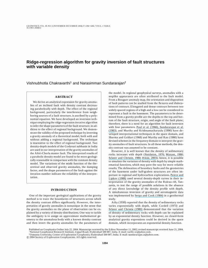
and z2 be the depths to the top and bottom of the fault, re-spectively, and the angle, i , be the angle subtended by the faultplane and the horizontal vector, extending in the direction ofthe downthrown block, as defined in Figure 1. Assume the ori-gin to be vertically above the inclined face of the fault plane.

Figure 1. Geometry of the fault model. Note that the fault angle, i , is defined with respect tothe horizontal vector extending in the direction of the downthrown block.

1396 Chakravarthi and Sundararajan

The analytical expression of gravity anomaly of such a faultstructure at any point, P (xk, 0), with density varying parabol-ically with depth, can be derived as

g(xk) = 2G∫ z2

u=z1

∫ ∞v=−(u−z1 cot i )

1ρ(u)udvdu

u2 + (v − x)2, (1)

where G is the universal gravitational constant, v, u are the co-ordinates of an elementary line mass having a cross-sectionalarea dvdu, and1ρ(u) is the density contrast of a section of thesedimentary sequence represented by the parabolic-densityfunction at a given depth, z= u, as described by Chakravarthiand Rao (1993) and Chakravarthi (1994):

1ρ(u) = 1ρ30

(1ρ0 − αu)2, (2)

where 1ρ0 is the density contrast extrapolated to the groundsurface, and α is a constant that can be obtained by fitting equa-tion 2 to the known density contrast-depth data of sedimentaryrocks. Using equation 2 in equation 1, the expression for gravityanomaly can be rewritten as

g(xk) = 2G1ρ30

∫ z2

u=z1

∫ ∞v=−(u−z1 cot i )

1(1ρ0 − αu)2

×[

udvdu

u2 + (v − x)2

]. (3)

On integration, equation 3 is simplified as

g(xk) = 2G1ρ30

Q

[(s1 + s2 + s3)

s6φ2 − (s1 + s4 + s5)

s7φ1

+ ssin(i ) lnr2s7

r1s6

], (4)

where

Q = 1ρ20 + 2s1ρ0 α cos(i )+ α2s2,

s = xk sin(i )− z1 cos(i ),

s1 = 1ρ0 scos(i ),

s2 = αs[s+ z2 cos(i )],

s3 = αz2,

s4 = αs[s+ z1 cos(i )],

s5 = αz1,

s6 = 1ρ0 − αz2,

s7 = 1ρ0 − αz1,

r1 =(xk + z2

1

)1/2,

r2 =([xk + (z2 − z1) cot(i )]2 + z2

2

)1/2,

φ1 = π/2+ tan−1(xk/z1), and

φ2 = π/2+ tan−1[(xk + (z2 − z1) cot(i )]/z2).

Here, φ1 and φ2 are the angles subtended by the radial vectorsr1 and r2 at the point of observation, P(xk, 0), as explained inFigure 1. The origin of the fault plane coincides with the originof the Cartesian coordinate system.

In practice, the gravity effect of a single fault structure sel-dom is isolated perfectly from its regional background of neigh-boring sources. In this paper, a polynomial (Nth degree) is usedto ascribe such interference. Therefore, in the presence of a re-gional background, equation 4 takes the form

g(xk) = 2G1ρ30

Q

[(s1 + s2 + s3)

s6φ2 − (s1 + s4 + s5)

s7φ1

+ ssin(i ) lnr2s7

r1s6

]+

N∑n=0

anxnk , (5)

where, an, are the coefficients of the polynomial. When thepoint of observation lies at the intersection of the extension ofthe fault plane and the x-axis, i.e., at xk= z1 cot(i ), equation 5reduces to

g(xk) = 2G1ρ30 (π − i )(z2 − z1)

s6s7+

N∑n=0

an[z1 cot(i )]n.

(6)Further, in the case of a concealed fault, the origin of the fault

plane, D, becomes an unknown parameter, in addition to z1,z2, and i . Paul et al. (1966) suggested an upward-continuationprocedure to locate the origin of the fault plane. In the caseunder discussion, the shape parameters (z1, z2, D, and i ) ofthe fault model are fixed with respect to an arbitrary referencepoint, R, (Figure 1) along the profile, and this could be realizedby replacing the terms containing xk by (X̂k− D) in equations 5and 6, where X̂k is the distance to the point of observation, P,from an arbitrary reference point, R, and D is the distance ofthe fault plane from R (Figure 1). Equations 5 and 6 are usedto compute the gravity anomalies, gmod(X̂k), of the theoreticalmodel. For α= 0, the parabolic-density function becomes con-stant. Hence, equations 5 and 6 can also be used to computethe gravity anomalies of a theoretical model with a constantdensity profile.

GRAVITY INVERSION OF FAULT MODELS

Gravity inversion of fault models is implicitly a mathemat-ical exercise that attempts to fit theoretical gravity anomaliesto the observed gravity anomalies employing the principles ofthe least-squares approach. For optimal values of parametersof the fault, the theoretical gravity anomaly mimics the ob-served anomalies based on the principles of inversion givenby Al-chalabi (1972). The process of inversion begins withcomputation of the theoretical gravity response of the initialmodel, defined by approximate values of model parameters.The values of initial parameters can be obtained either fromthe knowledge of known geology or from characteristic curves(Grant and West, 1965; Rao and Murthy, 1978). The differ-ences between observed and computed gravity anomalies arethen used to improve the model parameters in an iterativeapproach by adopting one of several optimization techniques(Box et al., 1969). The theoretical gravity anomalies gmod(X̂k)are computed using equations 5 and 6, for X̂k 6= z1 cot(i ) andX̂k= z1 cot(i ), respectively. The deviation of the observed grav-ity anomalies, gobs(X̂k), from the theoretical ones, gmod(X̂k), canbe expressed in a truncated Taylor’s series expansion involvingpartial derivatives of the anomaly; four increments of the shapeparameters, namely, dz1, dz2, d D and di ; and N increments of

Gravity Inversion of Fault Structures 1397

the coefficients of the regional background. It is given as

gobs(X̂k)− gmod(X̂k) = ∂g(X̂k)∂z1

dz1 + ∂g(X̂k)∂z2

dz2

+ ∂g(X̂k)∂D

d D+ ∂g(X̂k)∂ i

di +N∑

n=0

∂g(X̂k)∂an

dan. (7)

Analytical expressions of the partial derivatives in equation 7are given in Appendix A.

Linear equations similar to equation 7 are constructed foreach point of observation, X̂k, on the anomaly and (4+ N) nor-mal equations corresponding to four shape parameters of thefault structure, and N coefficients of the regional backgroundare framed and subsequently solved for the respective incre-ments by minimizing the quantum of misfit function defined by

J =Nobs∑k=1

[gobs(X̂k)− gmod(X̂k)]2, (8)

using the ridge-regression iterative algorithm (Marquardt,1963). Here, Nobs is the number of observations on the profileand (4+ N)≤ Nobs.

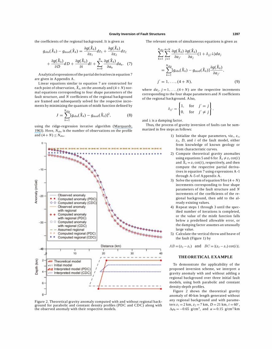
Figure 2. Theoretical gravity anomaly computed with and without regional back-ground for parabolic and constant density profiles (PDC and CDC) along withthe observed anomaly with their respective models.

The relevant system of simultaneous equations is given as

Nobs∑k=1

4+N∑j=1

∂g(X̂k)∂aj ′

∂g(X̂k)∂aj

(1+ δ j j ′λ)daj

=Nobs∑k=1

[gobs(X̂k)− gmod(X̂k)]∂g(X̂k)∂aj ′

,

j ′ = 1, . . . , (4+ N), (9)

where daj , j = 1, . . . , (4+ N) are the respective incrementscorresponding to the four shape parameters and N coefficientsof the regional background. Also,

δ j j ′ =1, for j ′ = j

0, for j ′ 6= j

,and λ is a damping factor.

Thus, the process of gravity inversion of faults can be sum-marized in five steps as follows:

1) Initialize the shape parameters, viz., z1,z2, D, and i of the fault model, eitherfrom knowledge of known geology orfrom characteristic curves.

2) Compute theoretical gravity anomaliesusing equations 5 and 6 for X̂k 6= z1 cot(i )and X̂k= z1 cot(i ), respectively, and thencompute the respective partial deriva-tives in equation 7 using expressions A-1through A-5 of Appendix A.

3) Solve the system of equation 9 for (4+ N)increments corresponding to four shapeparameters of the fault structure and Nincrements of the coefficients of the re-gional background, then add to the al-ready existing values.

4) Repeat steps 1 through 3 until the spec-ified number of iterations is completed,or the value of the misfit function fallsbelow a predefined allowable error, orthe damping factor assumes an unusuallylarge value.

5) Calculate the vertical throw and heave ofthe fault (Figure 1) by

AB = (z2− z1) and BC = |(z2− z1) cot(i )|.

THEORETICAL EXAMPLE

To demonstrate the applicability of theproposed inversion scheme, we interpret agravity anomaly with and without adding aregional background over three initial faultmodels, using both parabolic and constantdensity-depth profiles.

Figure 2 shows the theoretical gravityanomaly of 40-km length generated withoutany regional background and with parame-ters z1= 2 km, z2= 7 km, D= 21 km, i = 60◦,1ρ0=−0.65 g/cm3, and α= 0.15 g/cm3/km

1398 Chakravarthi and Sundararajan

Tabl

e1.

Ana

lysi

sof

grav

ity

anom

alie

sfo

rdi

ffer

entm

odel

sus

edin

the

inte

rpre

tati

onof

theo

reti

cala

ndfie

ldex

ampl

es.

Inte

rpre

ted

para

met

ers

wit

hP

DC

The

oret

ical

exam

ple

Inte

rpre

ted

para

met

ers

wit

hC

DC

Mis

fitM

isfit

func

tion

func

tion

(PD

C)

(CD

C)

Init

ialp

aram

eter

s

z 1z 2

Di

z 1z 2

Di

Num

ber

ofz 1

z 2D

iN

umbe

rof

Mod

el(k

m)

(km

)(k

m)

(deg

.)(k

m)

(km

)(k

m)

(deg

.)it

erat

ions

Init

ial

Fina

l(k

m)

(km

)(k

m)

(deg

.)it

erat

ions

Init

ial

Fina

l

∗ I1.

56.

519

.050

2.0

7.0

21.0

6018

1255

0.0

2.8

4.1

21.5

2440

1937

230.

1II

1.0

5.0

17.0

502.

07.

021

.060

1828

250.

02.

84.

121

.524

3012

6114

0.1

III

0.5

3.0

16.0

202.

07.

021

.060

2631

110.

02.

84.

121

.524

2741

489

0.1

The

oret

ical

exam

ple

(wit

hre

gion

alba

ckgr

ound

)∗ I

1.5

6.5

19.0

502.

07.

021

.060

1663

40.

02.

84.

121

.524

4018

3697

0.1

(−2.

12)

(37E−5

)(1

E−6

)(−

3.59

)(−

0.03

8)(6

5E−5

)II

1.0

5.0

17.0

502.

07.

021

.060

1919

250.

02.

84.

121

.524

2811

8032

0.1

(−2.

12)

(37E−5

)(1

E−6

)(−

1.48

)(3

9E−3

)(7

E−4

)II

I0.

53.

016

.020

2.0

7.0

21.0

6024

2265

0.0

2.8

4.1

21.5

2429

3686

70.

1(−

2.12

)(3

7E−5

)(1

E−6

)(−

1.48

)(3

9E−3

)(7

E−4

)

Fiel

dex

ampl

e∗ I

1E-4

3.0

16.5

800.

014.

0816

.26

110

9331

40.

170.

191.

8416

.01

127

2530

060.

2(−

2.28

)(−

0.20

38)

(0.0

024)

(−3.

56)

(−0.

29)

(−.0

07)

II1E

-33.

516

.590

0.01

4.15

16.2

710

8.2

9317

40.

10.

191.

8416

.01

127

1855

700.

2(−

1.71

)(−

0.13

)(0

.000

5)(−

3.56

)(−

0.29

)(−

.007

)II

I0.

013.

016

.570

0.02

4.15

16.2

511

193

295

0.3

0.19

1.84

16.0

112

740

3348

0.2

(−1.

86)

(−0.

17)

(0.0

07)

(−3.

56)

(−0.

29)

(−.0

07)

∗ Sho

wn

grap

hica

llyin

Figu

res

2,3,

4,6,

and

7.Fi

gure

sin

pare

nthe

ses

are

valu

esof

the

coef

ficie

nts

ofth

ere

gion

alba

ckgr

ound

.

Gravity Inversion of Fault Structures 1399

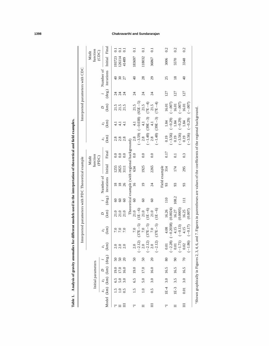
for both parabolic and constant density profiles at an interval of1 km. To invert the profile, the values of1ρ0 and α are derivedbased on density-depth information, and the values of otherinitial parameters, i.e., z1= 1.5 km, z2= 6.5 km, and i = 50◦

(model I of Table 1) are obtained from characteristic curvesof Rao and Murthy (1978). The value of the fourth parameter,D, is taken near the inflection point of the gravity profile, i.e.,at 19 km (Figure 2). The anomaly is subjected to inversion us-ing the strategy outlined with a predefined allowable error of0.0 mGal. Forward modeling is realized through equations 5and 6, where the regional background is ascribed by a secondorder polynomial a0+a1x+a2x2 (considering N= 2 in equa-tions 5 and 6). The regional gravity field with broad wavelengthcan be approximated by a second-order polynomial; hence, thechoice of such an interference term is justified.

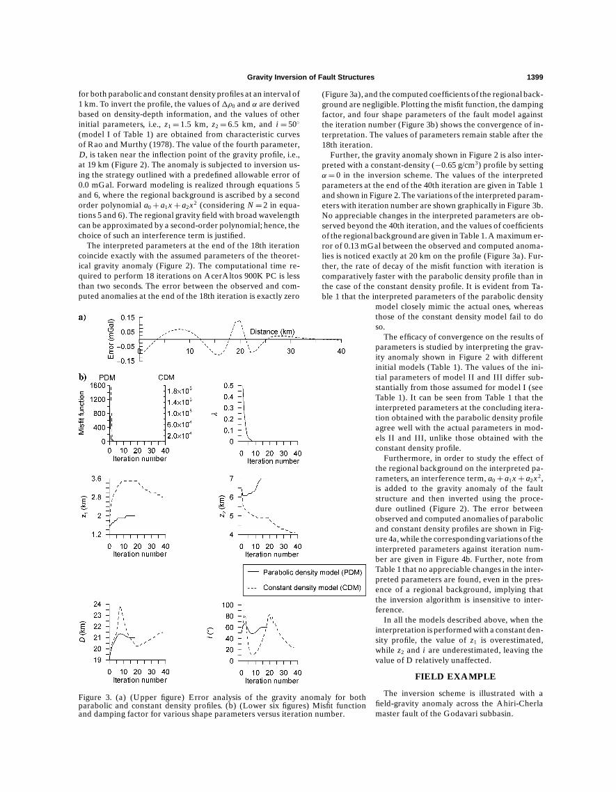
The interpreted parameters at the end of the 18th iterationcoincide exactly with the assumed parameters of the theoret-ical gravity anomaly (Figure 2). The computational time re-quired to perform 18 iterations on AcerAltos 900K PC is lessthan two seconds. The error between the observed and com-puted anomalies at the end of the 18th iteration is exactly zero

Figure 3. (a) (Upper figure) Error analysis of the gravity anomaly for bothparabolic and constant density profiles. (b) (Lower six figures) Misfit functionand damping factor for various shape parameters versus iteration number.

(Figure 3a), and the computed coefficients of the regional back-ground are negligible. Plotting the misfit function, the dampingfactor, and four shape parameters of the fault model againstthe iteration number (Figure 3b) shows the convergence of in-terpretation. The values of parameters remain stable after the18th iteration.

Further, the gravity anomaly shown in Figure 2 is also inter-preted with a constant-density (−0.65 g/cm3) profile by settingα= 0 in the inversion scheme. The values of the interpretedparameters at the end of the 40th iteration are given in Table 1and shown in Figure 2. The variations of the interpreted param-eters with iteration number are shown graphically in Figure 3b.No appreciable changes in the interpreted parameters are ob-served beyond the 40th iteration, and the values of coefficientsof the regional background are given in Table 1. A maximum er-ror of 0.13 mGal between the observed and computed anoma-lies is noticed exactly at 20 km on the profile (Figure 3a). Fur-ther, the rate of decay of the misfit function with iteration iscomparatively faster with the parabolic density profile than inthe case of the constant density profile. It is evident from Ta-ble 1 that the interpreted parameters of the parabolic density

model closely mimic the actual ones, whereasthose of the constant density model fail to doso.

The efficacy of convergence on the results ofparameters is studied by interpreting the grav-ity anomaly shown in Figure 2 with differentinitial models (Table 1). The values of the ini-tial parameters of model II and III differ sub-stantially from those assumed for model I (seeTable 1). It can be seen from Table 1 that theinterpreted parameters at the concluding itera-tion obtained with the parabolic density profileagree well with the actual parameters in mod-els II and III, unlike those obtained with theconstant density profile.

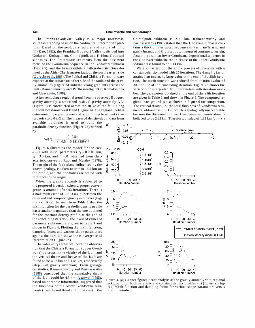
Furthermore, in order to study the effect ofthe regional background on the interpreted pa-rameters, an interference term, a0+a1x+a2x2,is added to the gravity anomaly of the faultstructure and then inverted using the proce-dure outlined (Figure 2). The error betweenobserved and computed anomalies of parabolicand constant density profiles are shown in Fig-ure 4a, while the corresponding variations of theinterpreted parameters against iteration num-ber are given in Figure 4b. Further, note fromTable 1 that no appreciable changes in the inter-preted parameters are found, even in the pres-ence of a regional background, implying thatthe inversion algorithm is insensitive to inter-ference.

In all the models described above, when theinterpretation is performed with a constant den-sity profile, the value of z1 is overestimated,while z2 and i are underestimated, leaving thevalue of D relatively unaffected.

FIELD EXAMPLE

The inversion scheme is illustrated with afield-gravity anomaly across the Ahiri-Cherlamaster fault of the Godavari subbasin.

1400 Chakravarthi and Sundararajan

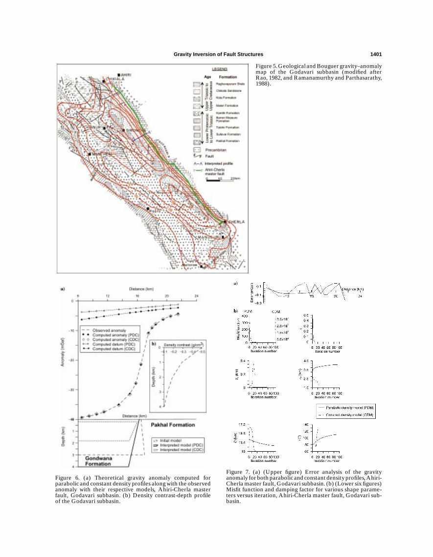
The Pranhita-Godavari Valley is a major northwest-southeast trending basin on the continental Precambrian plat-form. Based on the geology, structure, and nature of lithicfill (Rao, 1982), the Pranhita-Godavari Valley is divided intoGodavari, Kothagudem, Chintalpudi, and Krishna-Godavarisubbasins. The Proterozoic sediments form the basementrocks of the Gondwana sequence in the Godavari subbasin(Figure 5), and the basin exhibits a half-graben structure de-fined by the Ahiri-Cherla master fault on the northeastern side(Qureshy et al., 1968). The Pakhal and Chikiala Formations areexposed at the surface on either side of the fault, and the grav-ity anomalies (Figure 5) indicate strong gradients across thefault (Ramanamurthy and Parthasarathy, 1988; Ramakrishnaand Chayanulu, 1988).

After removing a regional trend from the observed Bouguergravity anomaly, a smoothed residual-gravity anomaly AA′

(Figure 5) is constructed across the strike of the fault alongthe southwest-northeast trend (Figure 6). The regional field isdetermined by equating areas of outcropping basement (Pro-terozoic) to 0.0 mGal. The measured density-depth data fromavailable boreholes is used to build theparabolic density function (Figure 6b) definedby

1ρ(z) = (−0.5)3

(−0.5− 0.1518259z)2.

Figure 6 illustrates the model for the caseα= 0 with initial parameters z1= 0.0001 km,z2= 3.0 km, and i = 80◦ obtained from char-acteristic curves of Rao and Murthy (1978).The origin of the fault plane, influenced by theknown geology, is taken nearer to 16.5 km onthe profile, and the anomalies are scaled withreference to the origin.

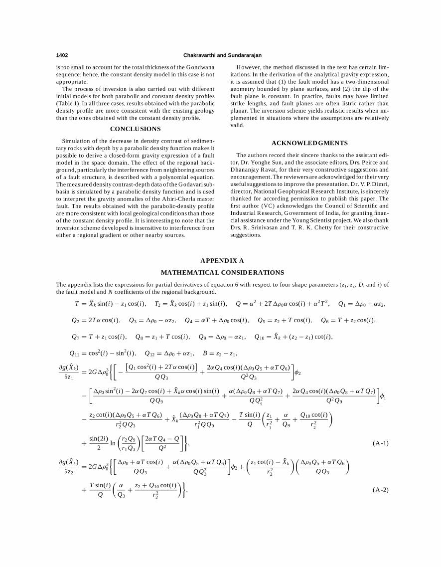
When the gravity anomaly is subjected tothe proposed inversion scheme, proper conver-gence is attained after 93 iterations. There isa maximum error of −0.23 mGal between theobserved and computed gravity anomalies (Fig-ure 7a). It can be seen from Table 1 that themisfit function for the parabolic-density profilehas a smaller magnitude than the one obtainedfor the constant density profile at the end ofthe concluding iteration. The inverted values ofparameters obtained are given in Table 1 andshown in Figure 6. Plotting the misfit function,damping factor, and various shape parametersagainst the iteration shows the convergence ofinterpretation (Figure 7b).

The value of z1 agrees well with the observa-tion that the Chikiala Formation (upper Gond-wana) outcrops in the vicinity of the fault, andthe vertical throw and heave of the fault arefound to be 4.07 km and 1.48 km, respectively(step 5 of gravity inversion). From geologi-cal studies, Ramanamurthy and Parthasarathy(1988) concluded that the cumulative throwof the fault could be 4.5 km. Agarwal (1995),based on borehole information, suggested thatthe thickness of the lower Gondwana sedi-ments (Kamthi and Barakar Formations) in the

Chintalpudi subbasin is 2.93 km. Ramanamurthy andParthasarathy (1988) stated that the Godavari subbasin con-tains a thick uninterrupted sequence of Permian-Triassic andpartly Jurassic and Cretaceous sediments of continental origin.Assuming a similar lower Gondwana depositional sequence inthe Godavari subbasin, the thickness of the upper Gondwanasediments is found to be 1.14 km.

We also carried out the entire process of inversion with aconstant-density model with 25 iterations. The damping factorattained an unusually large value at the end of the 25th itera-tion. The misfit function was reduced from its initial value of3006 to 0.2 at the concluding iteration. Figure 7b shows thevariation of interpreted fault parameters with iteration num-ber. The parameters obtained at the end of the 25th iterationare given in Table 1 and shown in Figure 6. The computed re-gional background is also shown in Figure 6 for comparison.The vertical throw (i.e., the total thickness of Gondwana sedi-ments) obtained is 1.65 km, which is geologically unacceptablebecause the thickness of lower Gondwana sediments alone isbelieved to be 2.93 km. Therefore, a value of 1.65 km (z2− z1)

Figure 4. (a) (Upper figure) Error analysis of the gravity anomaly with regionalbackground for both parabolic and constant density profiles. (b) (Lower six fig-ures) Misfit function and damping factor for various shape parameters versusiteration number.

Gravity Inversion of Fault Structures 1401

Figure 5. Geological and Bouguer gravity–anomalymap of the Godavari subbasin (modified afterRao, 1982, and Ramanamurthy and Parthasarathy,1988).

Figure 6. (a) Theoretical gravity anomaly computed forparabolic and constant density profiles along with the observedanomaly with their respective models, Ahiri-Cherla masterfault, Godavari subbasin. (b) Density contrast-depth profileof the Godavari subbasin.

Figure 7. (a) (Upper figure) Error analysis of the gravityanomaly for both parabolic and constant density profiles, Ahiri-Cherla master fault, Godavari subbasin. (b) (Lower six figures)Misfit function and damping factor for various shape parame-ters versus iteration, Ahiri-Cherla master fault, Godavari sub-basin.

1402 Chakravarthi and Sundararajan

is too small to account for the total thickness of the Gondwanasequence; hence, the constant density model in this case is notappropriate.

The process of inversion is also carried out with differentinitial models for both parabolic and constant density profiles(Table 1). In all three cases, results obtained with the parabolicdensity profile are more consistent with the existing geologythan the ones obtained with the constant density profile.

CONCLUSIONS

Simulation of the decrease in density contrast of sedimen-tary rocks with depth by a parabolic density function makes itpossible to derive a closed-form gravity expression of a faultmodel in the space domain. The effect of the regional back-ground, particularly the interference from neighboring sourcesof a fault structure, is described with a polynomial equation.The measured density contrast-depth data of the Godavari sub-basin is simulated by a parabolic density function and is usedto interpret the gravity anomalies of the Ahiri-Cherla masterfault. The results obtained with the parabolic-density profileare more consistent with local geological conditions than thoseof the constant density profile. It is interesting to note that theinversion scheme developed is insensitive to interference fromeither a regional gradient or other nearby sources.

APPENDIX A

MATHEMATICAL CONSIDERATIONS

The appendix lists the expressions for partial derivatives of equation 6 with respect to four shape parameters (z1, z2, D, and i ) ofthe fault model and N coefficients of the regional background.

T = X̂k sin(i )− z1 cos(i ), T2 = X̂k cos(i )+ z1 sin(i ), Q = α2 + 2T1ρ0α cos(i )+ α2T2, Q1 = 1ρ0 + αz2,

Q2 = 2Tα cos(i ), Q3 = 1ρ0 − αz2, Q4 = αT +1ρ0 cos(i ), Q5 = z2 + T cos(i ), Q6 = T + z2 cos(i ),

Q7 = T + z1 cos(i ), Q8 = z1 + T cos(i ), Q9 = 1ρ0 − αz1, Q10 = X̂k + (z2 − z1) cot(i ),

Q11 = cos2(i )− sin2(i ), Q12 = 1ρ0 + αz1, B = z2 − z1,

∂g(X̂k)∂z1

= 2G1ρ30

{[−[Q1 cos2(i )+ 2Tα cos(i )

]QQ3

+ 2αQ4 cos(i )(1ρ0 Q5 + αT Q6)Q2 Q3

]φ2

−[1ρ0 sin2(i )− 2αQ7 cos(i )+ X̂kα cos(i ) sin(i )

QQ9+ α(1ρ0 Q8 + αT Q7)

QQ29

+ 2αQ4 cos(i )(1ρ0 Q8 + αT Q7)Q2 Q9

]φ1

− z2 cot(i )(1ρ0 Q5 + αT Q6)r 2

2 QQ3+ X̂k

(1ρ0 Q8 + αT Q7)r 2

1 QQ9− T sin(i )

Q

(z1

r 21

+ α

Q9+ Q10 cot(i )

r 22

)

+ sin(2i )2

ln(

r2 Q9

r1 Q3

)[2αT Q4 − Q

Q2

]}, (A-1)

∂g(X̂k)∂z2

= 2G1ρ30

{[1ρ0 + αT cos(i )

QQ3+ α(1ρ0 Q5 + αT Q6)

QQ23

]φ2 +

(z1 cot(i )− X̂k

r 22

)(1ρ0 Q5 + αT Q6

QQ3

)

+ T sin(i )Q

(α

Q3+ z2 + Q10 cot(i )

r 22

)}, (A-2)

However, the method discussed in the text has certain lim-itations. In the derivation of the analytical gravity expression,it is assumed that (1) the fault model has a two-dimensionalgeometry bounded by plane surfaces, and (2) the dip of thefault plane is constant. In practice, faults may have limitedstrike lengths, and fault planes are often listric rather thanplanar. The inversion scheme yields realistic results when im-plemented in situations where the assumptions are relativelyvalid.

ACKNOWLEDGMENTS

The authors record their sincere thanks to the assistant edi-tor, Dr. Yonghe Sun, and the associate editors, Drs. Peirce andDhananjay Ravat, for their very constructive suggestions andencouragement. The reviewers are acknowledged for their veryuseful suggestions to improve the presentation. Dr. V. P. Dimri,director, National Geophysical Research Institute, is sincerelythanked for according permission to publish this paper. Thefirst author (VC) acknowledges the Council of Scientific andIndustrial Research, Government of India, for granting finan-cial assistance under the Young Scientist project. We also thankDrs. R. Srinivasan and T. R. K. Chetty for their constructivesuggestions.

Gravity Inversion of Fault Structures 1403

∂g(X̂k)∂ i

= 2G1ρ30

{[X̂k Q1 Q11 + z1 Q1 sin(2i )+ 2αT T2

QQ3

− (1ρ0 Q5 + αT Q6)(2X̂k1ρ0αQ11 + 21ρ0αz1 sin(2i )+ 2α2T T2)Q2 Q3

]φ2 −

[X̂k Q11 Q12 + z1 Q12 sin(2i )+ 2αT T2

QQ9

− (1ρ0 Q8 + αT Q7)(2X̂k1ρ0αQ11 + 21ρ0αz1 sin(2i )+ 2α2T T2)Q2 Q9

]φ1 − (1ρ0 Q5 + αT Q6)

QQ3

Bz2 cos ec2(i )r 2

2

− T BQ10

Qr22 sin(i )

+[

X̂k sin(2i )− z1 Q11

Q− (2X̂k1ρ0αQ11 + 21ρ0αz1 sin(2i )+ 2α2T T2)T sin(i )

Q2

]ln

r2 Q9

r1 Q3

},

(A-3)

∂g(X̂k)∂D

= 2G1ρ30

{[−Q1 cos(i ) sin(i )− 2αT sin(i )QQ3

− (1ρ0 Q5 + αT Q6)[− α1ρ0 sin(2i )− 2α2T sin(i )

]QQ9

]φ2

−[−Q12 cos(i ) sin(i )− 2αT sin(i )

QQ9− (1ρ0 Q8 + αT Q7)

[− α1ρ0 sin(2i )− 2α2T sin(i )]

Q2 Q9

]φ1

− z2

r 22

(1ρ0 Q5 + αT Q6)QQ3

+ z1

r 21

(1ρ0 Q8 + αT Q7)QQ9

+ T sin(i )Q

[X̂k

r 21

− Q10

r 22

]

− ln(

r2 Q9

r1 Q3

)[Q sin2(i )+ T sin(i )

[α1ρ0 sin(2i )− 2α2T sin(i )

]Q2

]}(A-4)

N∑n=0

∂g(X̂k)∂an

=N∑

n=0

(X̂k)n. (A-5)

REFERENCES

Agarwal, B. P., 1995, Hydrocarbon prospects of the Pranhita-Godavarigraben, India: Proceedings of Petrotech, 95, 115–121.

Al-chalabi, M., 1972, Interpretation of gravity anomalies by non-linearoptimization: Geophysical Prospecting, 10, 1–15.

Athy, L. F., 1930, Density, porosity and compaction of sedimentaryrocks: Bulletin of the American Association of Petroleum Geology,14, 1–24.

Box, M. J., D. Davies, and N. H. Swann, 1969, Non-linear optimizationtechniques: Oliver and Bayd Publishers.

Chai, Y., and W. J. Hinze, 1988, Gravity inversion of an interface abovewhich the density contrast varies exponentially with depth: Geo-physics, 53, 837–845.

Chakravarthi, V., 1994, Gravity interpretation of non-outcropping sed-imentary basins in which the density contrast decreases parabolicallywith depth: Pure and Applied Geophysics, 145, 327–335.

Chakravarthi, V., and C. V. Rao, 1993, Parabolic density function insedimentary basin modeling: 18th Annual Convention and Seminaron Exploration Geophysics, Expanded Abstracts, A16.

Cordell, L., 1973, Gravity anomalies using an exponential density-depth function—San Jacinto Graben, California: Geophysics, 38,684–690.

Garcia-Abdeslem, J., 1992, Gravitational attraction of a rectangularprism with depth-dependent density: Geophysics, 57, 470–473.

Grant, F. S., and G. F. West, 1965, Interpretation theory in appliedGeophysics: McGraw-Hill, Inc.

Hinze, W. J., 2003, Bouguer reduction density. Why 2.67?: Geophysics,68, 1559–1560.

Litinsky, V. A., 1989, Concept of effective density: Key to grav-ity depth determinations for sedimentary basins: Geophysics, 54,1474–1482.

Marquardt, D. W., 1963, An algorithm for least squares estimationof nonlinear parameters: Journal of the Society of Industrial andApplied Mathematics, 11, 431–441.

Maxant, J., 1980, Variation of density with rock type, depth, and for-mation in the Western Canada basin from density logs: Geophysics,45, 1061–1076.

Murthy, I. V. R., and D. B. Rao, 1980, Interpretation of gravity anoma-lies over faults and dykes by Fourier transforms, employing end cor-rection: Geophysical Research Bulletin, 18, 95–110.

Murthy, I. V. R., and S. K. G. Krishnamacharyulu, 1990, Automaticinversion of gravity anomalies of faults: Computers and Geoscience,4, 539–548.

Nettleton, L. L., 1976, Gravity and magnetics in oil prospecting:McGraw-Hill, Inc.

Paul, M. K., S. Dutta, and B. Banerjee, 1966, Direct interpretation oftwo dimensional structural faults from gravity data: Geophysics, 31,940–948.

Peirce, J. W., and L. Lipkov, 1988, Structural interpretation of theRukwa Rift, Tanzania: Geophysics, 53, 824–836.

Qureshy, M. N., N. Krishna Brahmam, S. C. Garde, and B. K. Mathur,1968, Gravity anomalies and the Godavari rift, India: GeologicalSociety of America, 79, 1221–1230.

Ramakrishna, T. S., and A. Y. S. R. Chayanulu, 1988, A geophysicalappraisal of the Purana basins of India: Journal of the GeologicalSociety of India, 32, 48–60.

Ramanamurthy, B. V., and E. V. R. Parthasarathy, 1988, On the evo-lution of the Godavari Gondwana Graben, based on LANDSATImagery interpretation: Journal of the Geological Society of India,32, 417–425.

Rao, C. S. R., 1982, Coal resources of Tamilnadu, Andhra Pradesh,Orissa and Maharashtra: Bulletin of the Geological Survey of India,2, 1–103.

Rao, B. S. R., and I. V. R. Murthy, 1978, Gravity and magneticmethods of prospecting: Arnold-Heinemann (India) PublishersInc.

Rao, P. R., and I. V. R. Murthy, 1989, Two Fortran 77 function subpro-grams to calculate gravity anomalies of bodies of finite and infinitestrike length with the density contrast differing with depth: Comput-ers and Geoscience, 8, 1265–1277.

Ruotoistenmaki, T., 1992, The gravity anomalies of two-dimensionalsources with continuous density distribution bounded by continuoussurfaces: Geophysics, 57, 623–628.

Sclater, J. G., and P. A. F. Christie, 1980, Continental stretching:An explanation of the post mid-Cretaceous subsidence of the

1404 Chakravarthi and Sundararajan

Central North Sea Basin: Journal of Geophysical Research, 85,3711–3739.

Serpa, L. F., and K. L. Cook, 1984, Simultaneous inversion of grav-ity and aeromagnetic data applied to a geothermal study in Utah:Geophysics, 49, 1327–1337.

Sharma, B., and L. P. Geldart, 1968, Analysis of gravity anomalies usingFourier transforms: Geophysical Prospecting, 16, 77–93.

Sundararajan, N., N. L. Mohan, and S. V. S. Rao, 1983, Gravity inter-pretation of 2D fault structures using Hilbert transforms: Journal ofGeophysics, 53, 34–41.