INFO - Oak Ridge National Laboratory
204
-
Upload
khangminh22 -
Category
Documents
-
view
0 -
download
0
Transcript of INFO - Oak Ridge National Laboratory


Printed in the United States of America. Available from National Technical Information Service
U.S. Department of Commerce 5285 Port Royal Road, Springfield, Virginia 22161
NTIS price codes-Printed Copy: ,410 Microfiche ,401
This report was prepared as an account of work sponsored by an agency of the UnitedStatesGovernment. NeithertheUnitedStatesGovernment noranyagency thereof, nor any of their employees, makes any warranty, express or implied, or assumes any legal liability or responsibility for the accuracy, completeness, or usefulness of any information, apparatus, product, or process disclosed, or represents that its usewould not infringe privately owned rights. Reference herein to any specific commercial product, process, or service by trade name, trademark, manufacturer, or otherwise, does not necessarily constitute or imply its endorsement, recommendation, or favoring by the United StatesGovernment or any agency thereof. The views and opinions of authors expressed herein do not necessarily state or reflect those of the United StatesGovernment or any agency thereof.

ORNL/CON-80/Rl
Contract No. W-7405-eng-26
Energy Division
'/ i
The Oak Ridge Heat Pump Models: I. A Steady-State Computer Design Model for Air-to-Air Heat Pumps
S. K. Fischer C. K. Rice
: DEPARTMENT OF ENERGY
Division of Building Equipment
, Date Published: Auqust 1983
OAK RIDGE NATIONAL LABORATORY Oak Ridge, Tennessee 37830
operated by UNION CARBIDE CORPORATION
for the DEPARTMENT OF ENERGY

. -

r TABLE OF CONTENTS
LIST OF FIGURES ................................................
LIST OF TABLES .................................................
ABSTRACT .......................................................
1. INTRODUCTION AND BACKGROUND ...............................
2. UTILIZATION ...............................................
3. CALCULATIONAL PROCEDURE AND ORGANIZATION .................. 3.1 Modeling Procedure for the Vapor Compression Cycle ... 3.2 Organization of the Computer Program ................. 3.3 Input and Output Description .........................
4. COMPRESSOR MODELS ......................................... 4.1 Introduction ......................................... 4.2 General Calculational Scheme ......................... 4.3 Map-Based Compressor Model ........................... 4.4 Loss and Efficiency-Based Compressor Model ...........
5. FLOW CONTROL DEVICES ...................................... 5.1 Introduction ......................................... 5.2 Capillary Tube Model ................................. 5.3 Thermostatic Expansion Valve Model ................... 5.4 Short Tube Orifice Model .............................
6. CONDENSER AND EVAPORATOR MODELS ........................... 6.1 Introduction ......................................... 6.2 Single-Phase Heat Transfer Coefficients in Heat
Exchanger Tubes ...................................... 6.3 Two-Phase Heat Transfer Coefficients in Heat Exchanger
Tubes ................................................ 6.4 Air-Side Heat Transfer Coefficients .................. 6.5 Heat Exchanger Performance ........................... 6.6 Fan Motor and Compressor Shell Heat Losses ...........
7. AIR-SIDE PRESSURE DROPS AND FAN POWERS ....................
8. PRESSURE AND ENTHALPY CHANGES IN REFRIGERANT LINES ........
vii
ix
1
3
7 *I
9
1: 16
37 37
z; 44
47 47
50
51 55
2:
65
Page
iii

Page
9. MODEL VALIDATION .......................................... 9.1 Introduction ........................................ 9.2 Compressor Modeling ................................. 9.3 Heat Exchanger Calibration .......................... 9.4 Heat Pump Validation at 5.4"C (41.7OF) Ambient 9.5 Heat Pump Validation at 10.6"C (51.0°F) Ambient'::::: 9.6 Cooling Mode Results ................................
10. RECOMMENDATIONS . . . . . . . . . . . . . ..*..........................
REFERENCES . . . . . . . . . . . . . . . . . . . . . . . . . . . . . . . . . . . . . . . . . . . . . . . . . . . . 85
APPENDIX A. DEFINITIONS OF INPUT DATA . . . . . . . . . . . . . . . . . . . . . . . .
APPENDIX B. SAMPLE INPUT AND OUTPUT DATA . . . . . . . . . . . . . . . . . . . . .
APPENDIX C. DEFINITIONS OF CONSTANTS ASSIGNED IN BLOCK DATA SUBROUTINE . . . . . . . . . . . . . . . . . . . . . . . . . . . . . . . . . . . . . . .
APPENDIX D. DEFINITIONS OF VARIABLES IN COMMON BLOCKS . . . . . . . .
APPENDIX E. CROSS-REFERENCE OF COMMON BLOCKS . . . . . . . . . . . . . . . . .
APPENDIX F. SUBROUTINE DESCRIPTIONS AND CROSS-REFERENCE OF SUBROUTINE CALLS . . . . . . . . . . . . . . . . . . . . . . . . . . . . . . . . .
APPENDIX G. ALGEBRAIC NOTATION . . . . . . . . . . . . . . . . . . . . . . . . . . . . . . .
APPENDIX H. DERIVATION OF DEHUMIDIFICATION SOLUTION . . . . . . . . . . H.l Introduction . . . . . . . . . . . . . . . . . . . . . . . . . . . . . . . . . . . . . . . . H.2 Heat Transfer Equations - Air to Wall . . . . . . . . . . . . . . . H.3 Heat Transfer Equations - Air to Mean Surface
Conditions . . . . . . . . . . . . . . . . . . . . . . . . . . . . . . . . . . . . . . . . . . H.4 Heat Transfer Equations - Mean Surface to Refrigerant
Conditions . . . . . . . . . . . . . . . . . . . . . . . . . . . . . . . . . . . . . . . . . . H.5 Derivation of Coil Characteristic and Total Heat Flow
Equation . . . . . . . . . . . . . . . . . . . . . . . . . . . . . . . . . . . . . . . . . . . . H.6 Derivation of the Solution for the Exit Effective
Surface Temperature, Tf, ,(x0) . . . . . . . . . . . . . . . . . . . . . . H.7 Derivation of the Soluti6n for the Exit Air Dry Bulb
Temperature T (x ) References for App%aixOH
. . . . . . . . . . . . . . . . . . . . . . . . . . . . . . . . . . . . . . . . . . . . . . . . . . . . . . . . . . . . . . .
APPENDIX I. DESCRIPTION OF THE DEHUMIDIFICATION ALGORITHM . . . . References for Appendix I . . . . . . . . . . . . . . . . . . . . . . . . . . . . . . .
APPENDIX J. RATIOS OF GEOMETRIC PARAMETERS USED IN HEAT EXCHANGER CALCULATIONS . . . . . . . . . . . . . . . . . . . . . . . . . . . .
73 73 73 74
:: 81
83
89
95
101
105
131
133
139
147 147 147
149
150
151
153
156 161
163 170
171
.
.
.
iv

Page .
APPENDIX K.
. APPENDIX L.
APPENDIX M.
.
.
APPENDIX N. LISTING OF THE MAP FITTING PROGRAM . . . . . . . . . . . . . . . 185
APPENDIX 0. SAMPLE COMPRESSOR MAP DATA . . . . . . . . . . . . . . . . . . . . . . . 185
APPENDIX P. LISTING OF THE INTERACTIVE SUBROUTINES . . . . . . . . . . . 185
APPENDIX Q. LISTING OF THE INTERACTIVE PREPROCESSOR . . . . . . . . . . 185
AVAILABILITY AND DISTRIBUTION OF THE HEAT PUMP MODEL . . . . . . . . . . . . . . . . . . . . . . . . . . . . . . . . . . . . . . . . . . . . 179
LISTING OF COMPUTER MODEL ........................ 185
SAMPLE INPUT DATA ................................ 185
V

.

LIST OF FIGURES
c Fig. 3.1
Fig. 3.2
Fig. 4.1
Fig. 4.2
Fig. 4.3
Fig. 6.1
Fig. 6.2
Fig. 6.3
Fig. 6.4
Fig. I.1
Fig. J-1
Pressure vs. Enthalpy Diagram for the Heat Pump Cycle . . . . . . . . . . . . . . . . . . . . . . . . . . . . . . . . . . . . .
Block Diagram of Iterative Loops in the Main Program . . . . . . . . . . . . . . . . . . . . . . . . . . . . . . . . . . . . . . .
Computational Sequence in the Compressor Models
Components of Compressor Energy Balance . . . . . . . .
Iteration on Internal Energy Balance for the Loss and Efficiency-Based Compressor Model . . . . .
General Structure of the Condenser Model . . . . . . .
General Structure of the Evaporator Model . . . . . .
Computational Sequence in the Condenser Model . .
Computational Sequence in the Evaporator Model . . . . . . . . . . . . . . . . . . . . . . . . . . . . . . . . . . . . . . . . . .
Block Diagram of the Dehumidification Algorithm
Sample Tube-and-Fin Heat Exchanger . . . . . . . . . . . . .
Page
10
15
21
27
31
48
49
57
58
164
172
vii

.
*
.
.
.

LIST OF TABLES
P
c Page .
c Table 9.1 Comparison of Experimental Data with Predictions of Compressor Map Model . . . . . . . . . . . . 75
Table 9.2 Heat Pump Model Validation at 5.4'C (41.7"F) Ambient . . . . . . . . . . . . . . . . . . . . . . . . . . . . . . . . . . . . . . . . 77
Table 9.3
Table 9.4
Table E-1
Table F-1
Heat Pump Model Validation at 5.4"C (41.7OF) Ambient Without Corrections to Compressor Map . . 79
Heat Pump Validation at 10.6OC (51°F) Ambient . . 80
Cross-Reference of Common Blocks . . . . . . . . . . . . . . . 132
Cross-Reference of Subroutine Calls . . . . . . . . . . . . 137
Table K-1 Sample Pages of Input Data for Interactive Version of Heat Pump Model . . . . . . . . . . . . . . . . . . ...183-184


.
The Oak Ridge Heat Pump Models: I. A Steady-State Computer Design Model for Air-to-Air Heat Pumps*
S. K. Fischer C. K. Rice
Energy Division Oak Ridge National Laboratory
Oak Ridge, Tennessee 37830
ABSTRACT
The ORNL Heat Pump Design Model+ is a FORTRAN-IV computer program to predict the steady-state performance of conventional, vapor compression, electrically-driven, air-to-air heat pumps in both heating and cooling modes. This model is intended to serve as an analytical design tool for use by heat pump manufacturers, consulting engineers, research institu- tions, and universities in studies directed toward the improvement of heat pump specify:
0
l
0
0
l
l
The model
performance. The Heat Pump Design Model allows-the user to
system operating conditions,
compressor characteristics,
refrigerant flow control devices,
fin-and-tube heat exchanger parameters,
fan and indoor duct characteristics, and
any of ten refrigerants.
will compute:
system capacity and COP (or EER),
compressor and fan motor power consumptions,
coil outlet air dry- and wet-bulb temperatures,
air- and refrigerant-side pressure drops,
a summary of the refrigerant-side states throughout the cycle, and
overall compressor efficiencies and heat exchanger effectiveness.
This report provides thorough documentation of how to use and/or modify the model. This is a revision of an earlier report containing miscellaneous corrections and information on availability and distribution of the model - including an interactive version.
*Research sponsored by the Office of Buildings and Community Systems, U.S. Department of Energy under contract W-7405-eng-26 with the Union Carbide Corporation.
'The ORNL Heat Pump Design Model was developed at Oak Ridge National Laboratory.
1

.
3
1. INTRODUCTION AND BACKGROUND
The ORNL Heat Pump Design Model is a Fortran-IV computer program
developed to predict the steady-state performance of conventional, vapor
compression, electrically-driven, air-to-air heat pumps in both heating
and cooling modes. The purpose for the development of this model is to
provide an analytical design tool for use by heat pump manufacturers,
consulting engineers , research institutions, and universities in studies
directed toward the improvement of heat pump efficiency.
The current model has evolved from programs written at ORNL [l,Z]
and at the Massachusettes Institute of Technology [3] and also makes use
of selected routines by Kartsounes and Erth [4], Flower [5], and Kusuda
[6]. The MIT model served as the starting point for heat pump modeling
at ORNL, where in 1978, the original program was modified and documented
in Ref. 1 as a preliminary version of the ORNL Heat Pump Model. An
improved version of this code was made available in 1979 with limited,
informal documentation. These two versions have been distributed to a
number of manufacturing ,and research institutions.
Our own use of the previous programs [7,8] as well as the experiences
of other users indicated the need for additional capabilities in the
model. Many of these needs were incorporated between 1979 and 1981.
This report is a revision of an earlier version with miscellaneous cor-
rections and additions. The places where corrections or additions have
been made are identified by vertical bars in the left margin. The philosophy of the model development has been to base the pro-
gram on underlying physical principles and generalized correlations to
the greatest extent possible, so as to avoid the limitations of empirical
correlations derived from manufacturers' literature. The correlations
and algorithms used in the previous releases of the model have been
critically reviewed and improved or replaced to include more recent or
appropriate correlations and more accurate and efficient algorithms.
The model has thus been significantly improved and expanded from the
earlier versions from an engineering standpoint. Furthermore, it has
been reorganized into a more modular format so that reseachers will
be able to readily adapt it to their specific needs.

4
The ORNL Heat Pump Design Model allows the user to specify:
e . System Operating Conditions II
0
0
0
0
l
1. the desired indoor and outdoor air temperatures and relative humidities, *
2 . . the arrangement of the compressor and fans in the air flow stream, i.e., up or downstream of the heat exchangers;
Compressor Characteristics
1. either a map-based model for designs with available equipment,
2. or an efficiency and loss model for advanced reciprocating compressors;
Refrigerant Flow Control Devices
1. a capillary tube, thermostatic expansion valve (TXV), or a short-tube orifice, or
2. a specified value of refrigerant subcooling (or quality) at the condenser exit (in this case the program calculates the equivalent capillary tube, TXV, and short-tube orifice parameters);
Fin-and-Tube Heat Exchanger Parameters
1. tube size, spacing, and number of rows, and number of parallel circuits,
2. fin pitch, thickness, and thermal conductivity; type of fins (smooth, wavy, or louvered),
3. air flow rates;
Fan and Indoor Duct Characteristics
1. overall fan efficiency values for indoor and outdoor fans, or
2. a specified fan efficiency curve for the outdoor fan,
3. the diameter of one of six equivalent ducts;
Refrigerants
1. either R12, R22, R114, or R502 as a standard option,
2. one of six additional refrigerants (Rll, R13, R21, R23, R113, and C318) by adding the appropriate thermodynamic constants given by Downing [9];

0 Refrigerant Lines
5
1. lengths and diameters of interconnecting pipes,
2. pipe specifications independent of heating or cooling mode,
3. heat losses from suction, discharge, and liquid lines.
The user cannot specify the system refrigerant charge; instead, it
is implicity assumed that the system is charged with the proper amount
of refrigerant for the specified operating conditions. This is a
satisfactory model for heat pump systems having a suction line accumulator
(charge-insensitive systems) which can store excess refrigerant and
maintain a low level of evaporator superheat.
For charge-sensitive systems, the performance with a given refrigerant
charge over a range of ambient temperatures cannot be accurately modeled
unless the level of evaporator superheat at each ambient temperature is
known. For such systems, however, single design point studies can still
be made.
The input and output of the program are-in English units. (The
model has evolved from computer codes that were based on the British
system of measurement and it would have been a major effort to convert
them to SI units). The specific units used for each input and output
parameter are given in Appendices A and B. Four output options allow
the user to control the amount of printed output. The basic program
output includes (as appropriate):
0 Capacity and COP
l
Compressor and fan motor power consumption
Sensible to total heat transfer ratio
Outlet dry- and wet-bulb temperatures
Air- and refrigerant-side pressure drops
Overall isentropic and volumetric compressor efficiencies
Heat exchanger effectiveness and UA values
Equivalent capillary tube, TXV, and short-tube orifice parameters
Summary of the refrigerant-side states throughout the cycle
Other levels of program output are discussed in Section 3.2 and
Appendix A.

6
This second generation heat pump model contains significant changes
from its predecessors and many additional capabilities. This report is
intended:
e to serve as a rigorous documentation (where appropriate) of the assumptions, correlations, and algorithms that are used by the program,
to provide a complete list of references from which data and equations were obtained, and
e to serve as a user's manual for those who will use the code intact and to aid those who will need to add new capabilities.
A basic understanding of vapor-compression air-to-air heat pumps has
been presumed for this report.

7
2. UTILIZATION
The physical specification of the heat pump and the indoor and
outdoor operating conditions are read from a single data file, as
described in Appendix A; tape drives and other peripherals are not
required. The program requires 56 K words of memory and typically
executes in less than 5 seconds on the IBM 3033 computer at ORNL. A
complete listing of the program is provided in Appendix K.
Although the Heat Pump Design Model is generally run as a stand-
alone program, it has been used in conjunction with other computer
software. An earlier version of the model has been used at ORNL with
numerical analysis and graphical display programs in heat pump design
optimization and parametric studies [7,8].

P
3. CALCULATIONAL PROCEDURE AND ORGANIZATION
3.1 Modeling Procedure for the Vapor Compression Cycle
The heat pump model is organized functionally into two major
sections. The first section combines the compressor, condenser, and
flow control device routines into an interrelated high-side unit. The
second section, the low-side unit, contains the evaporator model.
Calculations proceed iteratively between these two sections until the
desired overall balance is obtained. The calculational scheme is
independent of whether the unit is operating in the heating or cooling
mode.
Figure 3.1 represents the basic vapor compression cycle, shown on
an exaggerated pressure-enthalpy diagram, that is modeled by the program.
The user is required to specify:
l the level of evaporator exit superheat (or quality),
l design parameters for a flow-control device or the level of condenser exit subcooling (or quality),
l condenser and evaporator inlet air temperatures,
l dimensions of components and interconnecting pipes, and
l heat losses from interconnecting pipes.
The user must also provide estimates for:
e the refrigerant saturation temperature at the evaporator exit,
l the refrigerant saturation temperature at the condenser inlet, and
e the refrigerant mass flow rate.
These three estimates are used as starting points for iterations. The
final results of the model do not depend on how well or how poorly these
values are chosen; however, better guesses will yield-shorter running
times.
High-Side Computations
The computations for the high-side system balance begin with the
refrigerant state at the exit of the evaporator (point a in Fig. 3.1),
which is defined by the specified superheat and the estimate of the

10
I(
.
a b C
d e f g
ORNL- DWG 81-4749
ENTHALPY
EVAPORATOR EXIT COMPRESSOR SHELL INLET COMPRESSOR SHELL OUTLET
CONDENSER INLET CONDENSER OUTLET
INLET TO EXPANSION DEVICE EVAPORATOR INLET
Fig. 3.1 Pressure vs. Enthalpy Diagram for the Heat Pump Cycle

11
saturation temperature. This point remains fixed for one iteration of
the compressor, condenser, expansion device, and evaporator calculations.
The compressor model uses state point a along with:
l the estimates of the refrigerant mass fl temperature at the condenser inlet, and
ow rate and saturation
l the specification of the dimensions and suction and discharge lines
heat losses for the
to calculate the state at the shell inlet, b, she1 1 outlet, c, and the
condenser inlet, d, as well as a new estimate of the mass flow rate.
Fixed Condenser Subcooling
The remainder of the high-side calculations depend on whether a
flow control device has been chosen or if a desired value of condenser
exit subcooling (or quality) has been specified. The latter case is
described first since it is simpler. The condenser submodel uses:
l the physical description of the heat exchanger,
l the calculated refrigerant mass flow rate,
0 the condenser inlet air temperature and relative humidity, and
l the refrigerant state at the condenser inlet, point d,
to evaluate the refrigerant state at the condenser outlet, e. The level
of condenser subcooling is computed from knowledge of state e, and
compared to the specified value. If the two values do not agree within
a fixed tolerance (see Appendix C), the saturation temperature at point
d, is changed (in effect specifying a new condenser entrance pressure),
and the compressor and condenser calculations are repeated.
Each time the condenser saturation temperature is changed, the
compressor model calculates a new refrigerant mass flow rate and new
states b, c, and d and the condenser model updates state e. Once the
desired condenser subcooling is achieved, the state at the flow control
device, f, is computed using:
l the state at the condenser exit, e, l the dimensions and heat loss for the liquid line, and
l the most recent calculation of the refrigerant mass flow rate.

Refrigerant state f and the mass flow rate are then used to calculate
the equivalent capillary tube, TXV, and short-tube orifice parameters
that would produce the specified subcooling.
Specified Flow Control Device
When condenser subcooling is specified, the system acts as if it
has a flow control device with an infinitely variable opening, that is,
the high-side system pressure is completely determined by the balance
between the heat rejection capability of the condenser (constrained by
the exit subcooling), and the refrigerant pumping capability of the
compressor. When a flow control device is specified, the high-side
pressure is controlled by the pressure drop characteristics of the
expansion device, so the flow control model must be coupled with the
compressor and condenser routines to achieve the proper high-side
balance. This balance must be found iteratively since the mass flow
rate characteristic of the flow-control device is dependent on the
refrigerant state at the entrance to flow control device which, in
turn, is found from the condenser model using the refrigerant mass
flow rate obtained from the compressor model.
The calculations to achieve a high-side balance with a specified
flow control device are similar to the case where condenser subcooling
is fixed. The states at the compressor shell outlet and condenser
inlet and outlet, states e, d, and e, are computed for the estimate of
the saturation temperature at the condenser inlet. Since the condenser
subcooling has not been specified, the calculations proceed to the
flow control device entrance where state f is evaluated using:
e the state at the condenser exit, e,
0 liquid line dimensions and heat loss, and
0 the computed compressor mass flow rate.
The refrigerant mass flow rate which the flow control device will pass
based on its entrance conditions is calculated using state f and, in
the case of a thermostatic expansion valve or short-tube orifice, the
low-side pressure at the evaporator entrance, point g. If the latter
is required, the pressure at point g is initially assumed to be equal

13
to that at point a (i.e., no pressure drop in the evaporator), and
then later calculations in the evaporator model are used to improve
the estimate. If the refrigerant mass flow rates of the compressor
and flow control device do not agree within a specified tolerance the
compressor, condenser, and expansion device calculations are repeated
with a new estimate of the saturation temperature at the condenser
entrance. Once the two mass flow rates are in agreement, a high-side
balance has been obtained. One cycle analysis can now be completed by
computing the evaporator performance.
Low-Side Computations
The evaporator, or low-side, computations are based on:
l the refrigerant condition at the evaporator exit, state a,
l the refrigerant enthalpy at the evaporator inlet, point g, and
l the refrigerant mass flow rate.
These values have all been computed based on the estimated saturation
temperature and specified superheat (or quality) at the evaporator
exit. The saturation pressure at the evaporator inlet, point g, and
the inlet air temperature which would yield the specified superheat at
the assumed exit saturation temperature are still unknown. The evaporator
model is executed iteratively, varying the inlet air temperature from
one execution to the next, to calculate a value of superheat at the
evaporator exit and a pressure drop across the heat exchanger (and
hence a saturation pressure at the inlet since the exit conditions are
fixed).
A system solution has been completed for some evaporator inlet
air temperature, though not necessarily the desired one, when the
calculated exit superheat agrees with the specified value within a
given tolerance. (The high- and low-side loops are repeated once if a
thermostatic expansion valve or a short-tube orifice is specified as
the flow control device to ensure that an accurate evaporator inlet
pressure is used during the high-side calculations.) The system
solution is found for the desired evaporator inlet air temperature by
changing the saturation temperature at the evaporator exit, point a,
14
and repeating the entire calculational process. This iteration on
state point a continues until the computed inlet air temperature
agrees with the desired value within a specified tolerance. The
sequence of calculations is summarized in Fig. 3.2. The evaporator
inlet air temperature is nearly a linear function of the exit refrigerant
saturation temperature so that usually only one or two iterations over
the outermost loop in Fig. 3.2 are required.
3.2 Organization of the Computer Program
Just as the calculations shown in Fig. 3.2 are divided into
distinct sections, subroutines to perform these computations are divided
into distinct modules. The calculation of the system high-side balance,
for example, requires computing the performance of the compressor,
condenser, and (optionally) the flow control device and then balancing
the output of these components and the interconnecting pipes with each
other. This is accomplished in the heat pump model using individual
subroutines, one for each task:
l modeling the compressor
l modeling the condenser
l modeling the flow control device
* iterating on condenser saturation temperature
In addition each of these subroutines calls other service routines to
perform inner iterations and calculate thermodynamic and thermophysical
properties, pressure drops , and heat transfer coefficients, etc.
(Appendix F contains a cross-reference of all subroutines called from
each subroutine.)
The advantages to this program structure are that:
0 separate and identifiable tasks are performed by each subroutine,
0 modules can be easily modified to make improvements, replaced to use models for a different component type, or added to increase system analysis capability
l familiarization with the code can be done at different levels, depending upon the needs of a specific user.

‘ r x I
ORNL-DWG 81-4741
READ INDOOR AND OUTDOOR AMBIENT TEMPERATURES AND ESTIMATES OF THE CONDENSING AND EVAPORATING
TEMPERATURES
TXV, CAP-TUBE ,OR ORFICE SPECIFIED SUBCOOLING
FIND THE CONDENSING TEMPERATURE T sti,o, WHICH BALANCES THE COMPRESSOR AND EXPANSION DEVICE MASS FLOW RATES
FIND THE CONDENSING TEMPERATURE T so+,e, WHICH GIVES THE SPECIFIED
SUBCOOLING
IENT TEMPERATURE
Fig. 3.2 Block Diagram of Iterative Loops in the Main Program

16
One consequence of this modular approach, however, is that a single
large program becomes many short subprograms with a large number of
variables passed between them through common blocks. Appendices D and
E are included as aides to identify variables used in common blocks
and to identify which common blocks are used to pass data between
which subroutines.
3.3 Input and Output Description
As part of the modularization of the program, almost all of the
data input and output are done by two subroutines. Appendix A contains
definitions of the input data and Appendix B contains sample input and
output. There are, however, other constants used by the model which
are not read as input data, and there are other levels of printed
output than that shown in Appendix B.
Parameters and physical constants (e.g., tolerance parameters,
refrigerant number, atmospheric pressure) which are unlikely to be
changed frequently from one use of the program to another are assigned
values in a single subroutine (BLOCK DATA) in order to reduce the
amount of data that the user must specify for each run. These parameters
are described in Appendix C so that the user can change them as necessary.
The printed output shown in Appendix B is a system summary and
contains results computed after the outermost loop in Fig. 3.2 has
converged. The program has three other output options, as defined in
Appendix A. The first option limits the output to only one page of
computed results which gives the COP and capacity of the heat pump and
a brief energy summary. The other two options are for diagnostic pur-
poses in cases where an iterative loop fails to converge or for use in
checking out the proper operation of the program after changes have
been made. Intermediate results in the computations are printed out
with either of these two options. An input variable, as defined in
Appendix A, is used to specify whether to print the abbreviated output,
the standard output summary as in Appendix B, a summary after completion
of each major iteration in Fig. 3.2, or continuous output throughout
the entire sequence of computations. Further, the output statements

17
in most of the subroutines are arranged so that detailed, diagnostic output
from a particular subroutine can be obtained by removing one or two
print control statements in that routine.


19
4. COMPRESSOR MODELS
4.1 Introduction
Since the compressor is the heart of a heat pump system and the
primary user of electrical power, accurate compressor modeling is important
to good system performance prediction. This criterion, however, must
be tempered by consideration of the type of information available to
most potential users of the program and of the different types of heat
pump studies in which the program may be used. For these reasons the
ORNL Heat Pump Design Model does not incorporate a subroutine which
rigorously models compressor performance using detailed hardware
design parameters. Instead, users can choose between two simpler
models depending upon their specific needs.
The first compressor model is based on the use of compressor
manufacturers' data (compressor maps) for a specific compressor or
compressor type; the model has built-in corrections to adjust for
levels of refrigerant superheat in reciprocating compressors which are
different from those for which the maps were generated. Although this
model was written for reciprocating compressors, it should be easy to
modify for use with rotary, screw, or centrifugal compressors.
Accurate simulation of existing compressors is possible with this
model.
The second model, a loss and efficiency-based compressor model,
is intended for use in heat pump design studies, e.g., to predict how
changes in compressor loss and efficiency terms affect system performance.
It can also be used to model compressor performance with a new refriger-
ant. This more general routine models the internal energy balances in
a reciprocating compressor using user-supplied heat loss and internal
efficiency values. This model cannot predict compressor performance
as accurately over the same range of operating conditions as the map-
based model without local adjustment of some of the input efficiency
and loss values. It is well suited, however, for studying internal
compressor improvements and interactions and their effect on system
performance about a particular design point.

20
4.2 General Calculational Scheme
Both compressor models have a number of calculations in common
and interact with the rest of the system model in the same way. The
general calculational scheme is discussed first, followed by descrip-
tions of those sections of the two routines which are different.
Both models are functionally dependent on the refrigerant saturation
temperature at the condenser entrance and the evaporator exit and on
the refrigerant superheat at the evaporator exit. Figure 4.1 shows
the sequence of calculations for either method of compressor simulation.
The current estimates of the condenser inlet and evaporator outlet re-
frigerant saturation temperatures are used to calculate the corresponding
refrigerant pressures at the evaporator exit and the condenser entrance.
The refrigerant state at the evaporator exit is identified using the
specified degree of evaporator superheat or quality and the calculated
evaporator exit pressure (from the estimated refrigerant saturation
temperature), from which the refrigerant temperature, enthalpy, entropy,
and specific volume are computed.
The pressure drops in the suction and discharge lines are computed
as described in Section 8 using the current estimates for the refrigerant
mass flow rate and average refrigerant temperatures in the lines. The
refrigerant state at the‘compressor shell inlet is then identified
using the calculated suction line pressure drop and the specified
(input) value of heat gain in the suction line.
From this point, each of the compressor models use different
procedures to calculate:
0 the refrigerant mass flow rate,
0 the compressor motor input power,
0 the compressor shell heat loss (optional), and
0 the refrigerant state at the compressor shell exit.
Finally the refrigerant state at condenser entrance is computed using
the previously calculated discharge line pressure drop and the specified
(input) value of discharge line heat loss.

21
ORNL-DWG Sb4745R
( COMP OR CMPMAP J
CALCULATE THE PRESSURES AT THE CONDENSER INLET AND THE EVAPORATOR OUTLET
c /
r 1
3 CALCULATE REFRIGERANT PROPERTIES AT THE EVAPORATOR EXIT
\ _I
r 1 , CALCULATE b P IN
. THE DISCHARGE LINE
AND TqcmpAND Pcut,cmp J
t 7
CALCULATE AP IN THE SUCTION LINE AND
Tin,cmp AND Pin,cmp
+
CALCULATE REFRIGERANT CONDITIONS AT THE SHELL INLET
I
LOSS AND EFFICIENCY-BASED MAP -BASED
6 t , . SUCTION GAS ENTHALPY ITERATION
CALCULATE AND CORRECT POWER AND MASS-FLOW
FROM FIG. 4.3 RATE FROM CURVE FITS
ti AND SHELL HEAT LOSS
CALCULATE THE REFRIGERANT STATE I AT THE SHELL OUTLET CALCULATE THE
i
1
REFRIGERANT STATE AT THE SHELL OUTLET
f .
I I CALCULATE THE REFRIGERANT STATE AT THE CONDENSER INLET
r CALCULATE NEW AVERAG TEMPERATURES AND
t- SPECIFIC VOLUMES IN THE COMPRESSOR LINES
CALCULATE OVERALL VOLUMETRIC, ISENTROPIC,AND SUCTION GAS HEATING EFFICIENCIES
\
i
END
Fig. 4.1 Computational Sequence in the Compressor Models

22
Upon completion of these calculations, new average temperatures
and specific volumes in the suction and discharge lines are computed.
These are used with the latest calculation of the refrigerant mass
flow rate to recalculate the suction and discharge line pressure
drops. The entire process is repeated, as shown in Fig. 4.1, until
the pressure drops agree within tolerances from one iteration to the
next.
After completion of the pressure drop iteration, compressor ef-
ficiency indices are computed. In both compressor models, two basic
efficiency indices are calculated - the overall isentropic compression
efficiency and the overall volumetric efficiency. The term "overall"
is used to refer to a value based on compressor shell inlet and (when
appropriate) shell outlet conditions.
The overall isentropic compression efficiency, nCm is given by
the equation
Q lil (h n "k
cm,ideal = r,actual outlet,isen -h ) inlet R (4.1)
cm cm,actual cm,actual
where i cm and mr represent compressor motor power and refrigerant mass
flow rate and h represents specific enthalpy. The term houtlet isen
represents the outlet specific enthalpy that would be obtained irom an
(ideal) isentropic compression process based on the refrigerant entropy
at compressor shell inlet and the refrigerant pressure at shell outlet.
Thus T-I cm represents the ratio of the minimum power required (to compress
a given refrigerant mass per unit time) to the actual required power.
It should be emphasized that the actual refrigerant enthalpy at shell
outlet, houtlets is not used in Eq. 4.1; were this the case, any
completely insulated compressor would have an ncm value of 1.0.
The overall volumetric efficiency, nvol, is given by
i til %ol = fi
r,actual _ r,actual 'inlet
r,ideal DS
(4.2)

23
where v inlet is the refrigerant specific volume at compressor shell
inlet, D is the total compressor displacement, and S is either the
rated compressor motor speed for the map-based model (e.g., 3450 or
3500 rpm) or the actual motor speed for the loss and efficiency model.
These two efficiency indices, ncm and nVol should not be confused
with similarly defined internal compressor efficiencies for the loss
and efficiency compressor model based on suction and discharge port
conditions as discussed in Section 4.4.
The next two sections describe the differences between the two
compressor models - differences in input requirements, calculational
methods, and resulting output.
4.3 Map-Based Compressor Model
The map-based compressor model uses empirical performance curves
for reciprocating compressors obtained from compressor calorimeter
measurements performed by the manufacturers. These performance curves
provide compressor motor power input, refrigerant mass flow rate
and/or refrigerating capacity as functions of "evaporator" saturation
temperature (i.e., at compressor shell inlet) for four to six "condenser"
saturation temperatures (i.e., at the compressor shell outlet).
Usually each performance map is generated for fixed values of
condenser exit subcooling and compressor inlet superheat. For some
maps, however, the superheat is allowed to vary with changes in
"evaporator" saturation temperature while the suction gas temperature
at compressor shell inlet is held constant. Given the condenser exit
subcooling and compressor inlet superheat or fixed suction gas temperature,
refrigerant mass flow rate values can be derived from refrigerating ,,
capacity data. A routine for performing these calculations is given
1 in Appendix N.
The map-based routine uses curve fits to the compressor motor
power input (kW) and the refrigerant mass flow rate (lbm/h) as functions
of compressor shell inlet and outlet saturation temperatures to model
the published performance data. The user must provide sets of coefficients;
Cl' c,, **a, for bi-quadratic functions of the form given by Eq. 4.3

24
for the power input and mass flow rate as functions of the inlet and
outlet saturation temperatures,
.
f(T outlet' T inlet) = '1 Tiutlet + '2 Toutlet + '3 TLet +
'4 TinIet + '5 Toutlet Tinlet ' '6 (4.3)
A short computer program which uses a least squares algorithm to
I compute these coefficients is listed in Appendix N. Except as noted
below, these coefficients will apply for only one particular compressor.
The user must also specify the total actual compressor displacement,
the rated compressor motor speed, and the fixed refrigerant superheat
or temperature at the compressor shell inlet (upon which the map is
based) for the compressor which is being modeled. The desired compressor
displacement is also an input parameter; this value is used by the
map-based model to scale the compressor performance curves linearly to
represent a compressor with the same general performance characteristics
as the original compressor but of a different capacity.
As noted earlier, the compressor maps and the biquadiatic
fits to them are strictly applicable only for the superheat level or
suction gas temperature for which they were generated. The map-based
model applies correction factors to the empirical curve fits to model
the compressor at actual operating conditions.
Dabiri and Rice [lo] presented a technique for correcting the
compressor motor power input, i
rate, m cm,map'
and the refrigerant mass flow
r,map for values of superheat or suction gas temperature other
than those for which the maps were generated. Equations 4.4 and 4.5
give their correction factors to account for non-standard superheat
values,
ril r,actual
= [l t F (Vmap v v
- 1)-J lil actual r ,maP (4.4)
25
and
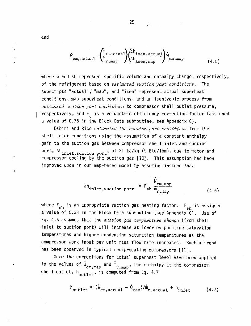
(4.5)
where v and Ah represent specific volume and enthalpy change, respectively,
of the refrigerant based on estimated suction port conditions. The
subscripts "actual", "map", and "isen" represent actual superheat
conditions, map superheat conditions, and an isentropic process from
estimated suction port conditCons to compressor shell outlet pressure,
1 respectively, and Fv is a volumetric efficiency correction factor (assigned
a value of 0.75 in the Block Data subroutine, see Appendix C).
Dabiri and Rice estimated the suction port conditions from the
shell inlet conditions using the assumption of a constant enthalpy
gain to the suction gas between compressor shell inlet and suction
port, Ah inlet,suction port , of 21 kJ/kg (9 Btu/lbm), due to motor and
compressor cooling by the suction gas [lo]. This assumption has been
improved upon in our map-based model by assuming instead that
.
Ah = inlet,suction port
Fs, +
r4w
where Fs, is an appropriate suction gas heating factor. Fsh is assigned
a value of 0.33 in the Block Data subroutine (see Appendix C). Use of
Eq. 4.6 assumes that the suction gas temperature change (from shell
inlet to suction port) will increase at lower evaporating saturation
temperatures and higher condensing saturation temperatures as the
compressor work input per unit mass flow rate increases. Such a trend
has been observed in typical reciprocating compressors [ll].
Once the corrections for actual superheat level have been applied
to the values of icm map and m r map, the enthalpy at the compressor
shell outlet, h outlei, is compuied from Eq. 4.7
h outlet
= (A cm,actual - 'can"'r actual + hinlet , (4.7)
26
where i,, is the heat loss rate from the compressor shell. i,, is
specified by the user as either a fixed input value or as a specified
fraction of actual compressor power, icrn actual. (Values of (j
are not usually provided by the compress& manufacturers.) can
The state at the compressor exit has been identified at this
point in the calculations and all the relevant thermodynamic properties
at the shell exit and condenser entrance are computed next. The
calculations then proceed to the outer pressure drop convergence loop
as described in Section 4.2.
4.4 Loss and Efficiency-Based Compressor Model
The loss and efficiency-based compressor routine models the
internal energy balances in a reciprocating compressor from user-
supplied design , internal efficiency, and heat-loss values. A conceptual
representation of the loss and efficiency-based compressor model is
shown in Fig. 4-2. The user is required to specify the following
values:
D -
c -
S input -
i s,fl -
n mot,max- n mech - n. - lsen
total compressor displacement,
actual clearance volume ratio,
synchronous or actual compressor motor speed (as appropriate),
compressor motor full load shaft power (optional),
maximum compressor motor efficiency,
compressor mechanical efficiency, and
isentropic compression efficiency from suction to discharge port.
The interna heat loss from the compressor discharge tube to the
low-side refrigerant gas, i hilo, and the compressor shell heat loss,
6 can, are also specified by the user according to the choices in Eqs.
4.8 and 4.9.
specified directly,
4 .
hilo = Qhilo 'cm,actual' or (see Appendix A) (4.8)
0.03 i cm,actual

27
ORNL-DWG 77-19443R
1
SUCTION - TUBE
my hsuction port
I I I I I -DISCHARGE
TUBE
hr houtlet
. mr hdischorge port
Fig. 4.2 Components of Compressor Energ.y Balance

28
I specified directly,
' = 'can 'cm,actual' Or (see Appendix A) (4.9)
can .
Oeg (lso - rlmotor 'mech) 'cm actual ,
The explicit losses, i, or fractions, ~1, are part of the input data to
' the program as described in Appendix A.
The unknowns which need to be calculated are:
i- refrigerant mass flow rate
h suction port enthalpy at the suction port
h discharge port
enthalpy at the discharge port
h outlet
enthalpy at the shell outlet
cl work done on the refrigerant r
ii work done on the shaft S
ii cm
work input to the compressor
4 cooling rate of heat loss due to cooling of compressor and motor
and if they are not specified explicitly, the:
6 can
'hilo
rate of compressor shell heat loss, and
rate of heat transfer from the discharge gas to the suction gas
These ten unknowns are calculated from the three energy bahace equations
in Eqs. 4.10 - 4.12,
(. (h suction port -h inlet) '= 'hilo + 'cooling -'can ' (4'10)
ir (h discharge port -h suction port )=c$ 3 (4.11)

29
and
'r (h outlet - hdischarge port) = -'hilo ' (4.12)
and the seven defining equations given in Eqs. 4.8 and 4.9 and Eqs. 4.13
through 4.17.
fir = I& (h -h isen,discharge port suction port )/(3413 nisenl 3
s = irhmech ,
B = 's'Tlmotor ' cm
il cooling =(1---l mech'motor"cm '
and
Ii =n S r vol,suction port oper D'u suction port
(4.13)
(4.14)
(4.15)
(4.16)
(4.17)
The combination of Eqs. 4.10 - 4.16 yields Eq. 4.18 for the overall
compressor energy balance,
i cm = ~~r(houtlet - hinlet) + EIcan1/34’3
c
which is identical to Eq. 4.7, the corresponding expression for the
map-based model. Equations 4.8 - 4.15 form a non-linear (through the
refrigerant properties), coupled set of equations where ir and mr are
dependent on hsuction port- The enthalpy at the suction port is
(4.18)

dependent
which can
The
equations
on mr and on theeheat
be dependent of W r’
1 osses, tcooling , thilo, and tcan. al 1 of
iterative calculational scheme used to solve this system of
is shown in Fig. 4.3. In order to begin the calculations,
I
30
h suction port is assumed to be equal to hinlet. Thereafter hsuction port
is calculated from the rearranged form of Eq. 4.10, given by Eq. 4.19.
h = suction port
h inlet + (0 hilo + 'cooling - 'can)"r (4.19)
The refrigerant conditions at the suction port are computed using
the values of h suction port
and the refrigerant pressure at the shell
inlet. Next, the refrigerant enthalpy at the discharge port is computed
using Eq. 4.20 (which combines Eq. 4.11 and 4.13),
h h
discharge port = h + isen,discharge port -h
suction port suction port(4.20) .
n. b. men
where h isen,discharge port
is the enthalpy after an isentropic compression
from the suction port conditions to discharge port pressure (assumed
equal to the shell outlet pressure).
Equation 4.20 contains the assumption that all the inefficiencies
in the compression process result in additional enthalpy gain for the
refrigerant gas. This is, of course, not theoretically correct since
the actual compression process is nonadiabatic (and is more properly
modeled as sequence of polytropic processes). There is heat transfer
from the compressor body to the refrigerant gas inside the compressor
shell. This extra heat loss is handled in a manner similar to that of
Davis and Scott [12], through an artifical increase in the mechanical
efficiency term in Eq. 4.16 above that which might be expected due to
frictional sources.
Once h discharge Dart
has been calculated, the remaining refrigerant
conditions at the discharge port are computed assuming the refrigerant
pressure at the discharge port is equal to that at the shell outlet.

31
ORNL- DWG 81- 4743
v a
.
CALCULATE THE REFRIGERANT CONDITIONS 4 AT THE SUCTION PORT
, I
c COMPUTE THE ENTHALPY AT THE DISCHARGE PORT AFTER ISENTROPIC COMPRESSION
1
J
+
COMPUTE I
SPECIFIED CALCULATED
+ c
CALCULATE THE COMPUTE MASS COMPRESSOR FLOW RATE OF MOTOR SPEED THE REFRIGERANT
4 4 c j \
COMPUTE REFRIG- DETERMINE WORK ERANT MASS Fu)W DONE ON THE RATE AND WORK REFRIGERANT DONE ON THE
< REFRIGERANT L /
r 4
,
4 \ ,
DETERMINE THE CALCULATE THE FRACTION OF FULL- FULL- LOAD MOTOR LOAD MOTOR POWER SHAFT POWER
\ /
0 I
CALCULATE THE COMPRESSOR MOTOR EFFICIENCY 1 \ , I
&r CONVERGENCE .
Fig. 4.3 Iteration on Internal Energy Balance for the Loss and
Efficiency-Based Compressor Model

32
The volumetric efficiency based on suction port conditions is computed
from Eq. 4.21 given by Davis and Scott [12].
n = vol,suction port,actual 'vol,suction port,theoretical -
-b
where
11 vol,suction port,theoretical = 1-c
(4.21)
P discharge port
- refrigerant pressure at discharge port
P suction port
- refrigerant pressure at suction port
Y - specific heat ratio for the specific refrigerant evaluated at suction port conditions
C - actual clearance volume ratio,
and "a" and "b" are empirical constants derived from test data for
compressors of different capacities but of the same series (defined in
Block Data). Davis and Scott [12] note that their equation should be
valid for "basically similar units which differ only in stroke or
clearance volume."
Once the volumetric efficiency has been evaluated, a decision
point is reached in Fig. 4.3. If the compressor-motor full load shaft
power, is fl, has not been specified as input data, the input values
of compreisor motor speed and efficiency are taken to be the actua2
operating values, i.e., S = S oper input and n motpr = 'motor max'
respectively. The refrigerant mass flow rate, m , the work input to
the refrigerant, i , and the required full load iotor power, is fl
are then computed from Eqs. 4.17, 4.13, and 4.14, respectively.' The
computed value for is fl is the rated (full) load that must be imposed
on the compressor motkr to achieve the assumed maximum rated motor
efficiency.

33
Alternatively, if is fl is specified as input data, the motor
speed, S oper' and efficie;cy, nmot , are computed as built-in functions
of fractional rated (full) load, f,,, as defined in Eq. 4.23.
f fl = 'r'(?nech 's,fl)
(4.23)
The operating motor speed, Soper, is assumed to be a linear function
of ffl, i.e.,
S oper = (l-0 + afl ffl) S sync (4.24)
where S sync
is the synchronous motor speed (e.g. 3600 or 1800 rpm) as
specified in the input data, i.e., S
The value of afl sync = S. .
is determined by solvi?::. 4.24 under full-
load conditions (f,, = 1.0) using known values of synchronous and
full-load motor speeds (i.e., afl = 'fl - 'sync). s
Since S is a function of i (tE%Ggh Eqs. 4.24, 4.23, and
4.13), and s%~ G is dependent onrS
not directly solva;rble for S oper (from Eq. 4.17), Eq. 4.24 is
. However,
used with Eqs. 4.13 and 4.1?':0' solve for S Eqs. 4.23 and 4.24 can be
oper algebraically. This results in Eq. 4.25,
S = oper
G&- afl ($)(g5J
where
60~1 vol,suction port D(l728v
suction port > 3
discharge port -h
suction port
(4.25)
(4.27)
34
and
f fl H iJ
= T/(3413 rlmech ws,fJ
r
(4.28) -
and the constants 1728 and 3413 are used to maintain consistent units.
Once 'oper has been evaluated from Eq. 4.25, values for 1; i r' r'
and ffl
are calculated from Eqs. 4.26, 4.27, and 4.28.
After ffl has been computed, the compressor motor efficiency can be
calculated from the,fit of motor efficiency to f,,, given by Eq. 4.29.
rl motor = n motor,max 5 'Imotor,i (ffl.'i (4.29)
i=O
The coefficients nmotor i in Eq. 4.29 are assigned values in the
Block Data subroutine (see Aipendix C). These coefficients were obtained
from a fit to data published by Johnson [13] for a motor with "medium"
slot size and maximum motor efficiency of 86% at a load of 6.8 N-m (80
oz-ft).
The next step in the calculations, after the compressor motor speed
and efficiency have been computed by one of these two methods and a
value has been calculated for i r, is to calculate the compressor power
input from Eq. 4.30.
GJ cm = fir/h mech'motor > (4.30)
The computed value of i is then used to evaluate 4 and
(optionally) ihilo and can cooling
using Eqs. 4.16, 4.8, and 4.9.
A new refrigerant enthalpy at the compressor suction port is cal-
culated using Eq. 4.19 and the sequence shown in Fig. 4.3 is repeated
until the change in the value of h suction port from one iteration to the
next is smaller than a specified tolerance. The refrigerant enthalpy at

35
compressor shell exit, houtlet, is then computed using Eq. 4.31 (a
rearranged form of Eq. 4.12),
d h hilo --
= hdischarge port hr (4.31)
outlet
After the associated refrigerant properties at the compressor shell
outlet and the refrigerant state and properties at condenser inlet have
been computed, the calculations proceed to the outer pressure drop con-
vergence loop described earlier in Section 4.2.
Once all of these iterative loops have converged, the loss and
efficiency-based model calculates a suction gas heating efficiency in
addition to the values of overall isentropic and volumetric efficiency
described in Section 4.2. The suction gas heating efficiency, nsh,
is defined by Shaffer and Lee [14] as
where
Ah isen,inlet
n = sh
F
and
Ah = isen,suction port
Ah isen,inlet
Ah isen,suction port
(4.32)
specific enthalpy change for an isentropic compression from she22 inZet conditions to shell outlet pressure
specific enthalpy change for an isentropic compression from suction port conditions to shell outlet pressure
The overall isentropic compression efficiency, no, is related to
rl sh by Eq. 4.33 [7,14-j.
11 = rl cm sh 'isen 'mech 'motor (4.33)
36
The terms on each side of Eq. 4.33 are thus computed independently. All
five efficiency terms in Eq. 4.33 are printed in the output for the loss
and efficiency-based model. These values serve as an independent check
on the compressor calculations and also to identify the relative
magnitude of the various compressor inefficiencies.
As a final note, the user must exercise caution in selecting
input values for n,,,h, nmOtoTP ihilo (orahilo), and iC, (oracan)
in the loss- and efficiency-based model. This is because certain
combinations of the four parameters can result in suction gas cooling
rather than heating between the compressor shell inlet and suction port.
This is an unrealistic situation and results in termination of the
program with a message "Inconsistent Data Set." Such a situation can
be checked for by the use of Eq. 4.10 and the requirement that the
suction gas enthalpy change be positive or zero, i.e.,
d hilo + 'cooling - 'can 2 '
Using Eq. 4.16 this gives
i hilo + (' - n,,,hn,oto,) w, - km 2 '
or, dividing through by i cm, an alternative expression is
(4.34)
(4.35)
(4.36)
37
5. FLOW CONTROL DEVICES
5.1 Introduction
The ORNL Heat Pump Design Model allows the user to specify a
fixed level of condenser subcooling or design parameters for a particular
expansion device in order to control the refrigerant flow between the
high and low sides of the system. The program contains subroutines
which employ correlations for capillary tubes, thermostatic expansion
valves (TXV), and short-tube orifices so that any of these three
devices can be modeled. In the event that condenser subcooling is
held fixed, each of these three submodels is called in such a way as
to compute the design parameters for an equivalent capillary tube,
TXV, and orifice that would produce the specified subcooling (this
involves using some assumed operating characteristics from BLOCK
DATA). When a flow control device is specified, the corresponding
model is used with the compressor and condenser models in an iterative
loop to obtain a balance between the calculated refrigerant mass flow
rate from the compressor and that through the expansion device as
described in Section 3.1.
5.2 Capillary Tube Model
One of the options in the Heat Pump Model is to simulate the
operation of one, or more, capillary tubes in parallel. The capillary
tube model requires the refrigerant pressure and degree of subcooling
at the inlet of the capillary tube or tubes. The model consists of
empirical fits to curves given in the ASHRAE Equipment Handbook [15]
for a standardized capillary tube flow rate as a function of inlet
pressure and subcooling for R-12 and R-22. The actual mass flow rate
through the capillary tube is given by
in r = +N
cap "k (5.1)

38
where
Ii; - standardized mass flow rate,
N - cap
number of capillary tubes in parallel,
@ - flow factor.
The capillary tube flow factor, 4, must be obtained from the ASHRAE
Equipment Handbook [15] for each particular combination of length and
inside tube diameter. The value of N is also required as input.
The standardized mass flow rate mi isciyven by Eq. 5.2 in terms of
inlet pressure, P, and two functions of the degree of subcooling, m 0
and k.
ii; P k
= m. 1500 ( > The coefficient, m o, and exponent, k, have been fit as functions of
subcooling, AT, as given by Eq. 5.3 and 5.4, such that mC agrees to
within 1.5% of the curves across the range of Fig. 40 in Ref. 15
3.56
m = 356 + 0.641 0
k = 0.4035 + 0.4175 e-0*04AT
(5.2)
(5.3)
(5.4)
In the situation where the Design Model is used with a specified
level of condenser subcooling in lieu of a specific flow control
device, the capillary tube correlations are used in such a way as to
compute the flow factor, 0, which would give the desired subcooling.
The capillary tube model used in the program assumes that the downstream
pressure is at or below critical pressure. However, Smith [16] has
fit additional curves in the ASHRAE Equipment Handbook [15] which could
be added by the user to predict capillary tube performance under non-
critical conditions.

39
The current model cannot handle incomplete condensation at the
capillary tube entrance. For all cases of incomplete condensation,
the subcooling is set to zero and calculations continue assuming that
1 the final conditions will have zero degrees of condenser subcooling.
If error messages are printed concerning "flashing in the liquid
line," the final results should be checked to make sure that the
refrigerant is not in a two-phase state at the capillary tube entrance.
If incomplete condensation is specified as input, the required value
for the flow factor 0 is set to zero.
5.3 Thermostatic Expansion Valve Model
The TXV subroutine contains: ,'
0 a general model of a cross-charged thermostatic expansion valve,
l specific empirical correlations for one size of distributor nozzle and tubes, and
l additional empirical equations to correct for nonstandard liquid line temperatures, tube lengths, and nozzle and tube loadings.
The general model of a cross-charged TXV is a form of the equation
used by Smith [16]:
ii =c r,TXV TXIJtAToper - ATstatic) (p??AplXV)1’2 (5.5)
been added, in keeping with the genera
equation. The remaining parameters in
lil r,TXV - mass flow rate that TXV
where a dependence on the refrigerant liquid line density, p,, has
1 form of the standard orifice
Eq. 5.5 are defined as follows:
will pass,
C TXV
- general orifice flow area coefficient,
AT oper - actual operating superheat,
AT static- static superheat (superheat at which the valve is just
barely open), and
AP TXV
- available pressure drop from TXVinlet to TXVexit.

40
The assumption of a cross-charged TXV valve implies that a given
AT oper'
at a given p, and AP,,,, will provide a certain valve opening
that is independent of evaporator pressure. Most TXV valves used in
the higher efficiency heat pumps are of the type described above since
such valves tend to maintain a relatively constant superheat over a
range of operating conditions.
If the actual operating superheat is greater than the maximum
effective superheat, *Tmax eff, where
ATmax eff = ATstatic + 1*33 (ATrated - ATstatic) , (5.6)
then ATmax eff is used in place of AT
oper in Eq. 5.5.
The flow area coefficient, C,,, and the available pressure drop
across the TXV valve, AP,,,, have to be calculated before Eq. 5.5 can
be used to compute a refrigerant mass flow rate. The value of CT,,
depends on four variables from the input data [17]:
6 rated' the capacity rating of the TXV valve (tons),
AT rated' the rated operating superheat of the valve (at 75% of
the maximum valve opening),
AT static'
defined earlier, and
b fat, the valve bleed factor.
The given capacity rating is used in conjunction with the bleed
factor and standard TXV rating conditions for a specific refrigerant
(specified in the Block Data routine) to calculate the rated refrigerant
mass flow rate:
f2,OOO 0 r-i
rated bfac = r,rated h
evap out,rated -h
liquid line,rated (5.7)
where
the constant 12,000 is used to convert from tons of capacity to
Btu/hr.

41
h evap out,rated is the evaporator outlet refrigerant enthalpy at
rated evaporator pressure and superheat,
and
h liquid line,rated is the refrigerant enthalpy at rated liquid
line temperature.
C TXV is calculated from Eq. 5.8 using mr rated: ,
Ii 'TX, = hT
r,rated --)(
rated static ,p ----TP- )V
r,rated rated (5.8)
where
P = r,rated
refrigerant density at rated liquid line temperature
and
AP = rated
rated pressure drop across expansion device.
The available pressure drop across the TXV valve, AP,,,, is the
remaining unknown in Eq. 5.5. This is computed using the ptfessures at
the TXV inlet and evaporator inlet and the pressure drops in the
distributor nozzle and tubes, i.e.,
aP TXV = P in,TXV -P
in,evap - APnoz - APtube (5.9)
The pressures Pin TXV and P. are computed elsewhere in the heat
pump model and ari input da~~'~~~pthe TXV routine. The nozzle and
tube pressure drops are calculated using specific empirica7Y fits
for one set of distributor nozzle and tube sizes for R-22 fZow and
additiona empirical equations to correct for non-standard liquid line
temperature, tube lengths, and distributor loading for R-22, 22, and
502. A,11 the equations were obtained from fits to published performance
data [18].
Distributor nozzles and tubes are often used with TXV's to equalize
the refrigerant flow in each evaporator circuit and to assure proper

42
TXV operation. At standard rating conditions the distributor nozzle will
have a pressure drop of 172 kPa (25 psi) for R-22 and R502 [103 kPa
(15 psi) for R-121 and the distributor tubes will each have
69 kPa (10 psi) drop. An input option has been provided which allows
the user to omit the nozzle and distributor tube computations for
specific applications to systems which do not have these components.
The first step in the evaluation of nPnoz and nPtube is the cal-
culation of the actual capacity of the nozzle, ~,,,, and of each tube
tj i.e., tube'
i no2 = r;lr(h
evap out,rated -h
liquid line,actual > (5.10)
0 tube = qnoz'Ncircuits (5.11)
where ", is the mass flow rate calculated by the compressor model and
N circuits is the number of circuits in the evaporator.
Next, the capacities are computed which yield the rated pressure
drops across the nozzles and tubes, i.e.,
cj,, rated = (3)12000 acor 10 (T
sat,evap - 40)/201.0
(5.12) ,
and
4 (T - 40)/177.64 tube,rated = (1.1)12000 aCOr .sor 10 sat*evaP (5.13)
where
the constants 3 and 1.1 are tonnage ratings from the equipment
specifications [18],
acor = correction factor for liquid line temperature other than lOO"F, i.e.,

43
a = lo(‘OO - Tin ,)/155.18
car I 10
(100 -Tin:,,,),140.19
T in,TXV '.'O" (5 ,4J
T in,TXV
,100 .
and
B = car
correction factor for tube lengths other than 30 inches, i.e.,
I3 car = (30/&be)1’3 (5.15)
Equations 5.12 and 5.13, respectively, represent the R-22 capacity of
a Sporlan [ll] nozzle No. 2.5 and l/4 inch OD copper tubes. FOP any
other nozzZe or tube, or refrigerant, Eqs. 5.22 and 5.13 must be
replaced (the correction terms acor and BcOr, Eq. 5.14 and 5.15,
do not need to be replaced).
Given the actual nozzle and tube capacities from Eqs. 5.10 and
5.11 and the rated capacities from Eqs. 5.12 and 5.13, the nozzle and
tube loadings
0 tube"
Lnoz and Ltube, defined as ~,,,/~,,, rated and
tube,rated respectively, and the nozzle and'tube pressure
drops, AP noz and aPtube, can be found.
For R-22 or R-502
I 25.0 (L )1.838
AP = noZ 0.9547 no2 29.4 (Lnoz)
L Il.2 no2
L > 1.2 (5.16) no2
AP tube
= 10.0(Ltube)'.8'22
For R-22 . AP = I 15.0(Lno2)'*8'7
noz 15.8l(L noz
)I.265 L noz
5 1.1
L > 1.1 (5.18)
noz

44
A!' = I
lo.o(Ltube)'.772 L tube ' l-6 (5.19)
tube 12.265(Ltube)1'3377 L tube >lS6
Equation 5.9 is then used to obtain AP, which, in turn, is used in
Eq. 5.5 to evaluated mr TXV.
In a case where a +ixed level of condenser subcooling is specified,
the subroutine calculates the required rated capacity of the TXV valve
from the equations
ii C TXV =
(AT - AT oper sta:ic)(","PTXV'1'2
(5.20)
ri r,rated = CTXV(ATrated - ATstatic)(Pr,ratedAPrated'1'2 (5*21)
6 = il r,rated(hevap out,rated - hliquid line,rated)
rated 12000 bfac (5 22) .
where AT oper
is replaced by ATmax eff from Eq. 5.6 if AToper > ATmax,eff
Or by ATrated if AToper 5 aT,t,ti~* The option to omit the nozzle and
tube pressure drop computations is also available when condenser sub-
cooling is specified.
The current model is not intended to handle incomplete condensation
at the TXV entrance. In such cases, the subcooling is set to zero and
calculations continue as described in the capillary tube case. If
incomplete condensation is specified, the program will set the TXV
rating values to zero.
5.4 Short Tube Orifice Model
The short-tube orifice subroutine which is included in the ORNL
Heat Pump Design Model uses correlations developed by Mei [19]. He
obtained data for five 0.127 m (0.5 in.) long Carrier Accurators
with diameters from 1.067 to 1.694 mm (0.0420 to 0.0667 inches) (L/D
ratios from 7.5 to 11.9) using R-22. He observed pressure drops

45
between 620 and 1515 kPa (90 and 220 psi) across the restrictor and
levels of subcooling from 0 to 28 Co (0 to 50 F") at the inlet. The
observed refrigerant mass flow rates ranged from 68.0 to 213 kg/h (150 to
470 lbm/h). The standard orifice relation in Eq. 5.23,
G r = $/Aorifice = c(2g PAP)"~ C
, (5.23)
was solved for the orifice coefficient C which was then correlated
with both the pressure drop across the short tube orifice, AP, and the
level of subcooling at the inlet, AT. Equation 5.24,
r;l = r
IID2 4
i
l-ID2 4
0.63683 - 0.019337 (P -P in in,evap q/2 + 0.006aT
I
x 2Prgc(Pin - 'in , for AT < 40
I[ 1 l/2 - 0.00325AT
2Prgc(Pin - 'in,sat)
for AT > 40 , (5.24)
was found to correlate the data to within 7.5% (with the maximum
difference occuring at low subcooling levels), where P in' P in,evap'
and P in,sat
are the pressures at the inlet to the orifice, the inlet
to the evaporator, and the saturation pressure at the inlet to the
orifice, respectively.
If the user has specified a fixed level of condenser subcooling
rather than selecting a particular flow control device Eq. 5.24 is
solved for the orifice diameter that would provide that subcooling.
As in the case of the other two models, if incomplete condensation is
specified, the corresponding orifice diameter is set to zero.

46
The user should always check that the computed refrigerant quality
at the flow control device entrance is equal to zero when using any of
the three flow control device models. If it is not, the calculated
results should not be used because the flow control models have been
extended beyond their intended range.
47
6. CONDENSER AND EVAPORATOR MODELS
6.1 Introduction
The ORNL Heat Pump Design Model calculates the performance of
air-to-refrigerant condensers and evaporators by using:
0 effectiveness vs. NtU correlations for heat transfer for a dry coil,
0 a modified version of the effective surface temperature approach when there is dehumidification,
0 the Thorn correlation for two-phase refrigerant pressure drops and the Moody friction factor chart plus momentum terms for the single- phase refrigerant pressure drop, and
0 friction factor equations for the air-side pressure drop for dry, partially wetted, or fully wetted coils.
Although the models for the condenser and evaporator are not identical,
the principal differences center around the dehumidification algorithm.
Since there are many similarities, the condenser and evaporator are
discussed together and the differences are pointed out where they
occur. The calculational methods which have been used assume that the
heat exchangers consist of equivalent, parallel refrigerant circuits
with unmixed flow on both the air and refrigerant sides [3]. The
refrigerant-side calculations are separated into computations for the
superheated and two-phase regions for the evaporator and for the
superheated, two-phase , and subcooled regions for the condenser.
Figure 6.1 is a general block diagram, or flow chart, outlining
the organization and iterative loops for the condenser model. Figure
6.2 is a similar diagram for the evaporator calculations.
The air-side mass flow rate for each heat exchanger is calculated
from the volumetric air flow rate specified in the input data and the
air density calculated from the ideal gas equation using atmospheric
pressure, the Universal gas constant for air (given in BLOCK DATA), and
the inlet air temperature. Since the heat exchangers are modeled as
several equivalent parallel refrigerant circuits (the actual number
being specified with the input data), the air-side mass flow rate and
the estimated refrigerant mass flow rate from the compressor model are
divided by the number of circuits to obtain values for each circuit.

48
ORNL-DWQ Sb4750R
.
CALCULATE AIR-AND REFRIGERANT- SIOE MASS FLOW k4TE PER CIRCUIT AND QEOMttRlC PARAMETERS
DETERMINE SUBCOOLED AND SUPERHEAlEO REFRlGERANt PROPERTIES AND REFRIQERANT- * SIDE HEAT TRANSFER COEFFICIENTS
4
DETEf3MI~E REFRIGERANT PROPER- TIES At@ HEAT TRANSFER ,3%F&IENT FOR TWO-PHASE
4 k
’ AOJUST THE TWO-PHASE HEAT TRANSER COEFFlCkNT FOR THE REQION WHERE THE BULK TEMPERATURE EXCEEDS THE SATURATION TEMPERATURE
COMPUTE AIR-SIDE PROPERTIES AND PRESSURE DROPS, OPTIONALLY ADD FAN AND/OR COMPRESSOR HEAT LOSS TO INCOMING AIR .AND COMPUTE AIR- SIDE HEAT TRANSFER COEFFICIENT
RETURN CODE
1'
Fig. 6.1
t v 1
COMPUTE REFRIGERANT- SIDE PRESSURE DROP FOR SUPERHEATED ,TWO-PHASE, AND SUGCOOLEO REGION
I
QPTIONALLY ADD FAN AND/OR COMPRESSOR HEAT LOSS TO OUTLET AIR AN0 COMPUTE UA VALUES
. General Structure of the Condenser Model

ORNL- DWG 864751
. f INITIALIZE ITERATION I
. I PARAMETERS 1 c f
CALCULATE AIR- AND REFRIGERANT- SIDE MASS FLOW RATE PER CIRCUIT AND GEOMETRIC PARAMETERS
DETERMINE SUPERHEATED REFRIGERANT PROPERTIES AND SUPERHEATED VAPOR * HEAT TRANSFER COEFFICIENT
t DETERMINE ENTERING QUALITY AND AVAILABLE HEAT TRANSFER IN THE TWO-PHASE REGION
*
DETERMINE REFRIGERANT PROPERTIES AND HEAT TRANSFER COEFFICIENT FOR THE TWO-PHASE REGION
L
CALCULATE AIR-SIDE PROPERTIES AND PRESSURE DROPS, OPTIONALLY ADD FAN AND/OR COMPRESSOR HEAT LOSS TO INCOMING AIR,AND COMPUTE
AIR-SIDE HEAT TRANSFER COEFFICIENT
COMPUTE REFRIGERANT-SIDE PRESSURE DROP FOR SINGLE AND TWO-PHASE REGION
A I
COMPUTE NEW AVERAGE + EVAPORATING
TEMPERATURE
OPTIONALLY ADD FAN AND/OR COMPRESSOR HEAT LOSS TO OUTLET AIR AND COMPUTE U A VALUES
Fig. 6.2 General Structure of the Evaporator Model

50
The average densities of the refrigerant liquid and vapor in the
two-phase region of each coil and the latent heat of vaporization are
calculated from the current estimates of the average saturation tem-
peratures in the heat exchangers. The thermophysical properties for
the single-phase refrigerant (subcooled and superheated for the condenser
and superheated for the evaporator), i.e., the viscosity, thermal
conductivity, and liquid specific heat, are calculated according to a
routine written by Flower [5]. The specific heat for the vapor region,
C p V, is determined by a routine developed by Kartsounes and Erth [4]
which computes the local value of ah at p = cp,vm
6.2 Single-Phase Heat Transfer Coefficients in Heat Exchanger Tubes
The refrigerant heat transfer coefficient for the superheated
region in the condenser is calculated (as reported in the MIT Model [3])
by Eq. 6.1.for gas flow from an abrupt contraction entrance [ZO] (h is used
throughout this report for heat transfer coefficients and h for enthalpy
variables).
h = C G c 1 r p,v *I+
-2/3 N '2 Re
(6.1)
where N, = GrD/p and,
1.10647 for 3500
c, -7
NRe <
= I 3.5194 x 10 for 3500 5 NRe < 6000 (6.2)
0.01080 for NRe 2 6000
-0.78992 for NRe < 3500
c, = 1.03804 for 3500 5 N Re < 6000 (6.3)
-0.13750 for NRe 2 6000

51
The constants used to define the step functions C1 and C2 defined in
Eqs. 6.2 and 6.3 are assigned in the BLOCK DATA subroutine (see
Appendix C).
The heat transfer coefficients for the subcooled region of the
condenser and the superheated region in the evaporator are computed
using the Dittus-Boelter correlation for fully developed flow [Zl]:
(6.4)
where "C" is 0.3 when the refrigerant is being cooling and 0.4
when being heated.
6.3 Two-Phase Refrigerant Heat Transfer Coefficients in Heat Exchanger Tubes
The two-phase heat transfer coefficients for the condenser and
the evaporator are average values obtained by effectively integrating
local values over the length of the two-phase region. The actual
integration is performed over the range of refrigerant quality [3]
where a length of tube dz is related to a change in quality of dx by
and AT is the change in temperature between the refrigerant and the
tube wall. Assuming that AT remains practically constant (as opposed
to assuming a constant heat flux) [3,22], the average heat transfer
coefficient, have, is given by
Z 0
s
X
h(x)dz x Odx
h = lz = i
ave
J
,
Z ' dz
i

which reduced to
The local heat transfer coefficient, h(x), for the condenser is
calculated as a function of the quality according to a correlation by
Travis [22].
I 0 9 F(Xtt) kl *Pr *Re ’ DF2
h(x) = 4
kL *Pr *Re
o g F(Xtt)1*15
’ DF2
where
F(Xtt) < 1.0
(6.5)
1.0 < F(Xtt) < 15
N = Gr D (1 -xJ
Re Yl ,
F(xtt) = 0.15 + 2.85Xtt-o'476 >
, and
(6.6)
(6.7)
(6.8)
F2 = F2 = 5.0 Npr 5.0 Npr + 5.0 lntl.0 + Npr(0.09636 NReo'585 -l.O)] + 5.0 lntl.0 + Npr(0.09636 NReo'585 - l.O)l
50 < N 50 < N < 1125 Re Re
< 1125
5.0 Npr 5.0 Npr + + 5.0 LnCl.0 +'5.0 NPr] + 2.5 1nC0.00313 NRe0s8121 5.0 Ln[l.O +'5.0 NPr] + 2.5 1nC0.00313 NRe0S812]
N N Re > 1125 (6.9) Re > 1125 (6.9) i
0.707 0.707 Npr NReoe5 Npr NReoe5 N N Re Re
c: 50 c: 50

53
The integration is carried out by a summation over steps of a constant
Ax and has been changed slightly from that in the Hiller and Glicksman
MIT Model [3]. The modifications pertain to the manner of extrapolating
to liquid and vapor heat transfer coefficients at the end points of the
integration. The average two-phase heat transfer coefficient is
adjusted using a correlation given by Rohsenow [23] for the region
where condensation (desuperheating) is occurring at the wall but the
bulk refrigerant temperature exceeds the saturation temperature. The
equation is
l/4 T
h = h v,ds -T
sat,in tP > (6.10)
P9v h fg
The bulk refrigerant temperature, TV ds, where refrigerant condensation
begins at the tube wall is calculated from Eqs. 6.11 and 6.12 where
v’T tp,in
-T T = a,in
v,ds r-l (6.11)
and
(6.12)
T tp,in and Ta in are the refrigerant temperature entering the two-
phase region And the inlet air temperature, respectively.
The average heat-transfer coefficient for the two-phase region of
the evaporator is derived from a correlation developed by Chaddock and
Noerager [24] for evaporation of refrigerant 12 in horizontal tubes
and from the general observations of Sthapak [25] for the dry-out
region. Equation 6.13 expresses the heat transfer coefficient in
terms of the local heat transfer coefficients as functions of refrigerant

54
quality from the inlet to the dry-out point, $(x) from xi to xdo,
and from dry-out to exit quality, h2(x) between xdo and x . 0
.
s 'do dx
X o dx
hlTx) + Xdo h2(x) h
1 - xi s
tP
s xxodx i
Examining the two integrals separately, hi(x) is given by Eq. 6.14
h&x) = 3*OhQ(Xtt 1 )2/3
. .
(6.13)
(6.14)
where Xtt is as defined in Eq. 6.6 and hL is the heat transfer coefficient
for liquid refrigerant obtained from Eq. 6.4. Thus
hi(X) = 3.0$(;;-) $1 'R l/3 'v 0.0667(; x x)O.6
V
and
J 'do
X i
k Xdo
J
(1 - x)06 dx xO.6
X i
(6.15)
where
Pt
3*0ht 0 -7
l/3 lJ 0 5
0.0667 V
C =
Equation 6.15 can be expanded, truncated, and integrated term by term to
yield

55
The second integral in the numerator of Eq. 6.13 is based on a
nonlinear interpolation of the heat transfer coefficient from the two-
phase value at the dry-out point, hl(xdo), from Eq. 6.14 to value of
pure vapor, h V'
from Eq. 6.4, i.e.,
h’ltxdo) - “VI (6.17)
where x do and x0 are refrigerant qualities at the dry-out point and the
outlet of the evaporator or the two-phase region (whichever comes first).
The second integral in Eq. 6.13 can be evaluated in closed form using
Eq. 6.17, i.e.,
/
X 0
+j-= (h, (Xdo)Ch (Xdo) - hvlF
2(xo - 'do) X
'do
{ hl(Xdo) Ch,fXdo) - h,])
{ h&xdo) b'l(xdo) - hvl}
(6.18)
A value of 0.65 is assumed for xdo in the model [25].
6.4 Air-Side Heat Transfer Coefficients
The air-side heat transfer coefficients are based on the work of
McQuiston [26,27], Yoshii [28], and Senshu [29] and are calculated by
the correlation given by Eq. 6.19.
C G c N _ -2'3 j 1
h = - 1280 N, NRe-lm2
a 0 a pa Pr 1 - 5120 NRe-ls2 1 (6.19)
where
j = 0.0014 + 0.2618 (, 1 FJ-o*15 (y ) -OB4 ,
N GawT Re= - I
lJ
and
C 0
= 1.0, 1.45, or 1.75 depending on whether the fins are smooth, wavy, or louvered (see Appendix G for parameter definitions).

/ 56
Equation 6.19 was obtained from extensive test data on smooth fins
over the Reynolds number range of 3,000 2 NRe 5 15,000. The heat
transfer coefficients for wavy and louvered fins are assumed to be
predicted approximately by the use of the smooth fin equation increased
by the multiplicative constant C . Data to verify this assumption
for a number of fin-and-tube geoietries, however, are not available.
The heat transfer coefficients so calculated for wavy and louvered fin
surfaces are assumed to be referenced to smooth-fin surface area; thus
the Co values for wavy and louvered fins are intended to account for
n
are
increases in both heat transfer coefficient and surface area from
smooth fin values. Equation 6.19 includes terms to adjust for a
number of geometric effects such as the number of tube rows, the f i
spacing, and the transverse tube spacing. The air-side properties
calculated using a modified version of a subroutine by Flower [5]
which is based on correlations published by the American Society o
Heating, Refrigeration, and Air Conditioning Engineers [30].
The air-side heat transfer coefficient for the portion of the
f
evaporator which is wetted due to dehumidification is calculated from
the dry coefficient, h a, by Eq. 6.20 from Myers [31].
h a,w = 0.626 ($)“.lolha (6.20)
The fin efficiency and overall surface effectiveness for.the con-
denser and for the dry region of the evaporator are calculated based
on the work of Schmidt [32] as reported by McQuiston and Tree [33] for
a tube surrounded by a hexagonal fin segment of a sheet fin (the
representative fin shape surrounding each tube in a staggered tube
arrangement). This work has been generalized to properly handle
orientation changes that occur as the longitudinal and transverse
tube spacings are varied.
6.5 Heat Exchanger Performance
Figures 6.3 and 6.4 are block diagrams for the subroutines which
calculate the performance of the condenser and evaporator, respectively.

57
ORNL-DWG El-4742R
CALCULATE THE REFRIGERANT
TEMPERATURE AT THE STARTOF THE DESUPERHEATING REGION
f COMPUTE THE EFFECTIVE 1 DRIVING ENTHALPY DIFFERENCE
FOR TWO-PHASE REGION
ITERATE TO FIND FRACTION OF COIL
IN VAPOR REGION
\\
f
f ”
COMPUTER FRACTION OF COIL IN TWO-PHASE REGION
f
> I tp SET ftp= 1 - f,
AND CALCULATE NO
THE EXIT QUALITY
1
SETf =f-(f tf,,
AND C&PUTE?,q AND
u& FOR SUBCOOLED
REGION 1
1
‘COMPUTE C, FROM ESTIMATED cp
FOR THE SUBCOOLED REGION
I t ,
CALCULATE EFFECTIVENESS AND NTU FOR SUBCOOLED REGION AND A NEW EXIT STATE
,
r \ CALCULATE A NEW
ESTIMATE OF cP
FOR THE SUECOOLED CONVERGENCE ON REGION
/
, CALCULATE HEAT TRANSFER
2. RATES AND EXIT AIR TEMPERATURE FOR EACH
\ FLOW REGION
Fig. 6.3 Computational Sequence in the Condenser Model

ORNL-DWG 81-4744R
CALCULATE PROPERTIES
OF MOIST AIR AND SUkFACE
EFFECTIVENESS AND THERMAL
RESISTANCE OF DRY COIL
COMPUTE AIR TEMPERATURE
WHEN DEHUMIDIFICATION
BEGINS, Toid
I
\ CALCULATE NTU AND
EFFECTIVENESS FOR
TWO-PHASE REGION
ASSUMING NO MOISTURE
REMOVAL OCCURS
COMPUTE EXIT AIR
TEMPERATURE FROM TWO-
PHASE REGION ASSUMING
NO MOISTURE REMOVED,
/ CALCULATE HEAT TRANS-
FER RATE AND THE YES MOISTURE
FRACTION OF THE COIL . REMOVAL OCCURS
SEE FIG.5.1
\ IN TWO-PHASE FLOW,f+P
I
ESTIMATE OF
AND COMPUTE
FOR THE VAPOR REGION
YES \ I
CALCULATE EXIT AIR IF “Jex,sat <Hi” THEN
CONDITIONS AND RATIO APPROXIMATE LATENT
c OF SENSIBLE TO TOTAL - HEAT REMOVED ASSUMING
HEAT TRANSFER < / , THATwo”t , = %x sat
Fig. 6.4 Computational Sequence in the Evaporator Model

In each case, the heat transfer for the liquid, vapor, and two-phase
refrigerant regions of the heat exchanger are computed using effective-
ness vs. NtU correlations, except for the two-phase refrigerant region
of an evaporator with dehumidification. If there is dehumidification
along the two-phase region of the evaporator, an effective surface
temperature approach is used as described in Appendices H and I.
Except for this case, the number of heat transfer units for the two-
phase region (condenser or evaporator) is given by Eq. 6.21,
(6.21)
where c is corrected for moist air conditions (i.e., c =c +
0.444*WPihere W is the air humidity ratio), and the effeFTiven& is
given by Eq. 6.22,
EtP = 1 - emN,u (6.22)
The numerator in Eq. 6.21, A , is the refrigerant-side heat transfer
area per unit of air mass flgw rate (see Appendix J).
When there is moisture removal on the evaporator, it is assumed
to occur only on the two-phase region of the coil. There is a check,
however, to ensure that the air leaving the superheated region of the
evaporator is not super-saturated. If this situation were to occur,
the humidity ratio and related values are changed to the appropriate
saturation values. Heat transfer in the case of dehumidification is
calculated using algorithms as described in Appendices H and I.
The air temperature for which dehumidification would occur at the
finned tube surface, Taid, is computed from the dew-point and saturation
temperatures, T dp
and Tsats using Eq. 6.23,
T = Tdp rl - Tsat
aid 5 -1 , (6.23)

60
where rl is given by Eq. 6.24
hA l-+22-
? = qd h A ' tp r
(6.24) .
T aid is used to determine whether or not dehumidification will occur as
is shown in Fig. 6.4.
The fraction of each coil with two-phase, superheated, and sub-
cooled refrigerant is needed to calculate the pressure drop and heat
transfer rate for each region. The computation of the fraction of the
condenser or evaporator containing two-phase refrigerant is based on
the heat transfer rate necessary to condense or evaporate all of the
refrigerant, which is given by Eq.6.25,
itp = I m h' r fg
r;lh r fg
for the condenser
for the evaporator (6.25)
where
h fg =
h tp,out
-h tp,in'
The driving enthalpy difference, hkg, for the condenser calculations
in Eq. 6.25 is given by Eq. 6.26,
h' fg
= h f g
tc p,V (TV,ds - Ttp,in)
(6.26)
where the bulk refrigerant temperature at which refrigerant condensation
begins at the tube wall [3],Tv dS,is computed from Eq. 6.11. The mass flow
rate of air necessary to achieie CjtP is then given by Eq. 6.27
il ‘tp a'tp = mip,S\.g -TEi,in /
(6.27)

61
and the fraction of the coil with two-phase refrigerant by Eq. 6.28
f = ma tp/“ia tP ,
(6.28)
If f for the evaporator is greater than 1, the entire coil contains
two-$ase refrigerant. If f tP
+ fv is greater than 1 for the condenser,
where fv is the fraction of the coil which is superheated (as described
later), then ftp is set equal to 1 - f .
The effectiveness of the superheaTed and subcooled regions is
calculated for a cross-flow heat exchanger with both fluids unmixed.
Since the exact solution is not in closed form, an approximate solution
developed by Hiller [3] is used.
The approximate solution uses equations for a counterflow heat
exchanger, i.e., Eq. 6.29,
1 - ewNtu(' - Cmin'Cmax) emNtutl - Cmin'Cmax) E = --
cf
C min < c max
C min = c max
(6.29)
in conjunction with Eq. 6.30 to correct for a cross-flow orientation.
E =E 1
V cf - C (1 + 0.047 p)(Ntu)0.036 Cmin'Cmax
(6.30)
max
The parameters C min and 'max are the minimum and maximum capacity rates
(mcp), respectively. The number of transfer units for the superheated
region is given by Eq. 6.31
N 1 =-
tu RCmin (6.31)
where the thermal resistance, R, is given by Eq. 6.32

62
where
R= f$ +2--
V rh V
(6.32)
The fraction of the evaporator in the superheated region is
simply whatever is not in two-phase, i.e.,
fv=l-f tP (6.33)
However, the average specific heat of the vapor, and thus the capacity
rate of the refrigerant vapor, C,, depends on the unknown exit refrigerant
temperature. Thus, the effectiveness and fraction of the coil in the
vapor region of the evaporator must be found as the result of an
iteration on the exit state.
The fraction of the coil in the superheated region of the condenser
requires one further iteration. Since all three refrigerant regions
can
and
by
occur
6.33.
iterati
in the condenser, fv cannot be calculated from Eqs. 6.28
The fraction of the condenser which is superheated is found
w on fv, and thus Cmax/Cmin, until Eq. 6.34 is satisfied, i.e.,
(6.34)
where
c l = m c f = c a a pm v min Or 'max ' (6.35)
The single-phase effectiveness vs. NtU relations, Eqs. 6.29-
6.32, are also used to calculate the effectiveness of the subcooled
fraction of the condenser, Ed, (fa. is necessarily used in place of

63
.
F
I
fv) * If there is liquid refrigerant at the condenser exit, f1 can be
calculated from the previously determined values of fv and f tP using
Eq. 6.36
I
f,=l-f -f tP v
(6.36)
.
and Ca calculated as in Eq. 6.35 with fV replaced by fg.
The refrigerant capacity rate, C ) depends on the average specific
heat for the subcooled region and henie on the unknown exit temperature.
Thus, the effectiveness and heat transfer rate for the subcooled
region are found by iterating on the exit temperature and average
specific heat for the liquid refrigerant.
The heat transfer rate for the entire coil is calculated as the
sum of the rates for the two-phase, subcooled, and superheated regions.
The heat transfer rate for the two-phase region is calculated according
to Eq. 6.25 while those for the single-phase regions are computed
using Eq. 6.37,
C tj=ri CAT .
r P r (6.37)
The air-side temperature change for each of the three regions is
determined using Eq. 6.38,
(6.38)
where 4 is sensible heat transfer only and both 6 and Ca pertain to
the particular region of the coil. The outlet air temperature from
either heat exchanger is calculated by Eq. 6.39,
T C'i
=T 4-y a,out a,in m c a Pm

64
where the summation is over the two or three refrigerant regions of
evaporator or condenser, respectively.
6.6 Fan Motor and Compressor Shell Heat Losses
Section 7 contains a discussion of the air-side pressure drops
and fan motor power consumption. The Heat Pump Design Model has an
option (specified with the input data) which allows the user to determine
whether or not fan motor or compressor-shell heat losses are added to
the incoming or exiting air for each heat exchanger. For blow-through
units, the fan heat is added to the air before it crosses the coil,
and hence before coil performance is computed. Alternatively, the fan
heat can be added after the air has crossed the coil for draw-through
units so that only the exit air temperature is affected. The compressor
placement in the air stream, i.e., before or after the heat exchanger,
can also be specified. If desired, the compressor shell and/or fan
heat losses can be omitted from the air temperature calculations.

65
7. AIR-SIDE PRESSURE DROPS AND FAN POWERS
The air-side pressure drop for the indoor unit is calculated as
the sum of pressure drops due to the ducts, filter, supplemental
heaters, and the coil and cabinet:
AP indoor
= AP ducts
+ A!' filter
+ AP heaters
+ AP coil and cabinet
The first three components are computed using the correlations given
in Eqs. 7.1 - 7.3 [34,35,36],
AP ducts
= 2.035 x 10 -8(o.a3613)$Y!! ducts
' AP filter = 6.75 x 10
AP -7
heaters = 1.027 x 10
where
(0.03613
'5 - the volumetric air-flow rate
(7.1)
(7.2)
2
(7.3)
A filter - the frontal area of the filter, and
A heater - the cross-sectional area of the resistance heater
section.
The constant aracks depends on the number of racks of heater elements
and is 1.0 for one or two racks, 2.0 for three racks, and 2.4 for four
racks.
The correlation [34] for the pressure drop across dry, wavy- or
louvered-fin coils depends on the fin type, the number of tube rows, N,,
.

66
the fin pitch, F P'
and the air face velocity, represented as the ratio
of the volumetric air flow rate to the frontal area, a/A, i.e.,
AP = coil & cabinet,dry
l.lO(O.03613) x lO-6 > 'a7 x
01
[
- 1.7 0.235 + 0.0638F g Xl P A
. (7.4)
The value of AP given from Eq. 7.4 is increased by 10% for louvered
fins as reported by Hosoda [37]. The pressure drop across the fraction
of the coil which is wet due to dehumidification is increased by a
factor w which is correlated to the gap (in mm) between fins [37], i.e.,
[l/F P
- 6-j.
w = 1.2 + 1.359 (l/Fp - 6)-o.5786
Thus
AP coil & cabinet
= AP coil & cabinet,dry l [(’ - Fw) + F,“l
where
(7.5) :
d
F = F f W w,tp tP
FW is the fraction of the evaporator air-side area wetted by dehumidi-
fication and F w,tP
is the fraction of the coil depth in the two-phase
region that is wetted.
The coil pressure drop for smooth fins is based on Fanning friction
factors for the dry and wet regions and correlating parameters FP and
F(s) defined by McQuiston [26,27]:
f dry = 0.004904 + 1.382 (FP)2
f wet
= 0.004904 + 1.382 [F(s) FP12,

67
. F(s) = (1 + N,-"*4)(~+)1.s, P
D GD
R* = 2(1 - F a
)LTS t
- Da)yp+lJ ' Andrea =2?&.
1-i a
Using the above correlations, the value Of APcoil & cabinet for smooth
dry or wet fins is given by Eq. 7.6,
1.10 f 62 AP
tot Amin a coil & cabinet = 2~~(32.174)(3600)~ (144)
where ftot is a weighted sum of the wet and dry Fanning
factors given by
f tot = fdry(l - Fw) + fwet Fw
, (7.6)
friction
(7.7)
The parameter Amin in Eq. 7.5 is the ratio of total air-side area to
minimum free-flow area. Note that the effect of the number of tube rows
is implicitly included in A min'
The 1.1 factor in Eqs. 7.4 and 7.6 is
to account for cabinet pressure drop. The air-side pressure drop for the outdoor unit contains only
components for losses due to the coil and cabinet. Equation 7.5 is
used to compute APoutdoor for a coil with smooth fins and Eq. 7.4 for
a coil with either wavy or louvered fins.
The fan motor power consumption, ifan,
Eq. 7.8,
.
is computed according to
(7.8) i ' APair fan
= 11.1 'fan,motor
where the constant is to convert to consistent units. The combined l fan and fan-motor efficiency, nfan motor, is a constant for the indoor
unit and can be held constant or ailowed to vary with the fan specific
speed for the outdoor unit. If the built-in outdoor fan curve is

68
selected (see Appendix A), the static efficiency of the fan is computed
according to Eqs. 7.9 and 7.10 as a function of the specific speed, S . S
S 17 =
static -3.993 + 4.266 log (lo;0 -) - 1.024 [log 2
10
where
S = S
Sfan(i)o’5 (ApH20)-o*75
(7.W
(7.10)
Equation 7.9 is for a representative propeller fan. The coefficients in
Eq. 7.9 are assigned in BLOCK DATA (see Appendix C) as well as a
representative fan speed of 825 rpm and fan motor efficiency of 55%.
The combined fan and fan-motor efficiency is given by Eq. 7.11,
'Ifan,moto7! .= 0.55 q
static (7.11)
An outdoor fan efficiency curve is provided as an option for the
outdoor coil because the outdoor coil and fan characteristics are
closely coupled. The indoor fan is less affected by the indoor coil
air-side pressure drop than by the rest of the indoor duct system.
Therefore, an after-the-fact selection of an indoor fan will not be
likely to result in any compatibility problems. Such a problem might
occur, however, in the outdoor coil , i.e., fan requirements may not be
easily met with current fans [8].
The various correlations for coil air-side pressure drops given
here are not widely verified nor well correlated (e.g., f 35% for
smooth fins). The smooth-fin correlation (for a dry condition) predicts
pressure drops some 20% higher than the wavy-fin equation. This is a
contradiction of the results of Yoshii [28] and of general expectations
regarding wavy fins vs. smooth fins. The wavy fin equations given by
Kirshbaum and Veyo [34], however, agree well with the results given by
Hosoda [37]. The user shouZd be aware of these inconsistencies and
should rely on experimental data specific to the application at hand
whenever possible.
69
8. PRESSURE AND ENTHALPY CHANGES IN REFRIGERANT LINES
All of the refrigerant-side pressure losses are computed on the
basis of equivalent lengths. The equivalent length and inside diameter
of each section of refrigerant piping, denoted by L, and D, respectively,
are specified as part of the input data (see Appendix A) for:
0 the liquid line from the condenser to the flow control device,
l the line from the outdoor coil to the reversing valve,
0 the line from the indoor coil to the reversing valve, and
0 the suction and discharge lines from the compressor shell inlet and outlet to the reversing valve.
and G
The rates of heat loss in the discharge and liquid lines, idis
liquid line , and the heat gain in the suction line, tsuction line,
can also be specified in order to allow enthalpy changes in the piping,
i.e.,
The line specifications are independent of operating mode.
Pressure and enthalpy changes in the suction and discharge lines and
lines from coils to reversing valve are calculated in the compressor
subroutines, COMP and CMPMAP, while the liquid line is modeled in
subroutine FLOBAL.
The Darcy incompressible flow relation, as given by Eq. 8.1, is
used to compute the pressure drop of the refrigerant in both the
compressor suction and discharge lines:
AP = 2f(L/‘J)G2 P ave
(8.1)
where f is the Moody friction factor. Thus, it has been assumed that
there are no significant density or momentum changes in these lines.

70
If there is two-phase flow in the suction line the pressure drop is
approximated by 190% of the pure vapor value, rather than iterating to
find the lengths of pipe having single-phase and two-phase flow. The
Moody friction factor, f, in Eq. 8.1 is computed using a subroutine
written by Hiller and Glicksman [3] and takes into account the surface
roughness of the tubes (see Appendix C).
The refrigerant-side pressure drops for the evaporator and con-
denser are calculated separately for the superheated, two-phase, and
subcooled regions of each coil. The pressure drop in the vapor region
is computed as the sum of changes due to momentum and friction effects
and due to losses in the return bends. The momentum component of the
pressure drop is given by Eq. 8.2,
AP =f G2 ( v. - vi,
v,mom (32.174)(3600)2 (144) (8.2)
where the plus sign is used for the evaporator and the minus sign for
the condenser. The Moody friction factor, f, and the equivalent
length of tubing in the vapor region, L/D, are used to compute the
pressure drop due to friction from Eq. 8.3.
G2 f(W) 2v AP
ave v,frict = (32.174)(3600)' (144)
(8.3)
where vave = (v + vi)/2. Finally, the pressure drop in the return
bends is computzd using Eq. 8.4 from Ito [38] where S, is the spacing
between tube passes and Nrb is the number of return bends in the vapor
region of the coil.
AP = v,rb 0.4338 [ 1 + 116 (& 'T -4.52, +)0.84
D
N -0.17
Re G* Nrb v ave --
(32.174)(3600)2 (144) (8.4)

71
It has been assumed that the density changes in the subcooled region
of the condenser are insignificant, so the pressure drop in the liquid
region only has friction and return bend components. These factors
are computed using Eqs. 8.3 and 8.4 with the properties and parameters
referring to the liquid refrigerant region rather than the vapor
region.
The pressure drop in the two-phase region of each heat exchanger
is calculated as the sum of momentum, friction, and return bend com-
ponents integrated over the two-phase region. The momentum and friction
terms are computed using equations from Thorn [39] as discussed by
Goldstein [40], that is,
AP = GL tp ,mom -- Cr,b,)
COpR - r,b,!l
and
AP tp ,frict = C2Cxor,ho) - Xir-j(xi)l
(8.5)
(8.6)
where
C 0
= (32.174)(3600)' (144),
c 1
= (x -x )/L 0 i tp'
0.184 NRe-'** G2 n
c, = 2Co&
,
r2(x) = acceleration multiplier tabulated by Thorn as a function of quality and steam pressure,
and
r&4 = frictional multiplier tabulated by Thorn as a function of quality and steam pressure.
The values of steam pressure in Thorn's tables [39] have been converted
to equivalent property index values where the property index is given
by Goldstein [40] as pi/p,. Double-quadratic interpolations are used
to obtain values of r2 and r3 as a function of quality and property index.
72
The total pressure drop in the return bends with two-phase flow
is computed using Eq. 8.7 an equation due to Geary [41].
5 . 58 10-6(N~ esat)
112xm(l.5708)($ G 2 e -0.215(ST/D) N
AP tp,rb =
rbytp (8.7) :. .-. -___ 2p, (32.174)(3600)2
where
x = m
(x2.25 -x2.25 0
i )/C2.Wxo - xi)1 (8.8)
73
9. MODEL VALIDATION
c
9.1 Introduction
Earlier versions of the ORNL heat pump model have been tested
[1,2,7] against data taken in our laboratory [42] to assess the accuracy
of the calculations. Since a number of air and refrigerant-side cor-
relations have been improved from the previous versions, a new validation
is needed. The present version has been validated against the same
data base [42] as previously used except for an important correction
to the experimental data. It was recently found by Miller [43] that
the rotameter used in the original experiment gave results which
underestimated the refrigerant mass flow rate by 5 to 20% (with the
larger errors occurring at lower mass flow rates) when compared to a
more accurate turbine flow meter. This finding is consistent with the
observations that
0 the air-side heating capacities in the original experiment were generally 5 to 15% higher than the refrigerant-side values,
0 the agreement between air and refrigerant-side values in Miller's experiment [43] using the turbine meter was within 4%, and
0 the refrigerant mass flow rates measured in Miller's experiment are within + 1% of the compressor map. value [lo].
Thus, in previous validations where the compressor model was "calibrated"
with experimental data, values of refrigerant mass flow rate that were
too low were used in the heat exchanger calculations. The geometry of
the low-bid test unit as described by Domingorena [42] and given in
the sample input in Appendix B is used for all validation runs discussed
here.
9.2 Compressor Modeling
Previous validations have been made using a "calibrated" loss and
efficiency-based compressor model. The loss and efficiency-based com-
pressor model, as discussed in Section 4, cannot model existing compressors
over a range of operating conditions as accurately as can the map-based

74
model. For this reason, the curves of a compressor map for the Tecumseh AH5540E compressor used in the laboratory unit were fit over the
operating conditions of interest (using the program in Appendix M) to
obtain coefficients for a biquadratic fit of compressor power and
refrigerant mass flow rate as functions of condensing and evaporating
saturation temperatures.
The predictions of the compressor map model, as reported by
Dabiri and Rice [lo], are shown in Table 9.1 and compared with the
"corrected" experimental data at the validation points to be considered
here. These tabulations show that the compressor map model slightly
overpredicts refrigerant mass flow rate and more significantly under-
predicts the required compressor input power.
Experimental data with which to compare the compressor map model
may not be available to many users of the heat pump model. For such
users, the errors of the magnitude shown in Table 9.1 and Ref. 10 must
be expected. However, if experimental data are available, the com-
pressor map equations can be refined to predict the performance of a
specific compressor more accurately by the use of multiplicative
correction constants.
9.3 Heat Exchanger Calibration
Such corrections to the compressor map equations were performed
for validation runs at ambient temperatures of 5.4"C (41.7OF) and
10.6"C (5l.OOF). By making such corrections, the accuracy of the heat
exchanger predictions can be examined independently of the accuracy of
the compressor model for the purpose of heat exchanger model calibration.
The heat exchangers on both the indoor and outdoor coil of the
laboratory test unit have wavy fin surfaces; however, the only general
air-side heat transfer correlations that are available [26,27] are for
smooth fins. Thus it was decided to adjust the air-side heat transfer
coefficient for smooth fins by a multiplicat
agreement in heating capacity (based on refr
was reached between model and experiment.
ive factor until good
igerant-side calculations 1
r

75
.
r
Table 9.1
Comparison of Experimental Data with Predictions of Compressor Map Model
Ambient Temperature
Calculated Observed % Difference
'C (OF) Value Value Calculated/Observed
Comparison of refrigerant mass flow rates
5.4 (41.7) 0.045 (359) 0.044 (351) 2.3 10.6 (51.0) 0.048 (379) 0.047 (371) 2.2
Compressor Power Input (watts)
5.4 (41.7) 3779 4090 -7.6 10.6 (51.0) 4011 4170 -3.8

76
9.4 Heat Pump Validation at a 5.4"C (41.7"F) Ambient
This procedure was carried out for the 5.4"C (41.7OF) ambient,
heating-mode case. Table 9.2 gives the results of the final validation
run with a multiplicative factor of 1.45 applied to the smooth-fin,
air-side heat transfer coefficient. This validation run and the
limited experimental results of Yoshii [28] form the basis for our
choice of a 1.45 factor for wavy fin geometry as discussed in Section
6. The model values for indoor and outdoor fan power consumptions
were set equal to the experimental values because the unit was tested
in atypical duct loops. Experimental values for the compressor shell
heat loss as a fraction of the compressor input power and the suction,
discharge, and liquid line heat transfer rates were also specified as
input data for the model. Thus, Table 9.2 is primarily a test of the
accuracy of heat exchanger models and the capillary tube model. Since
the air-side heat transfer coefficient was uniformly adjusted until
the calculated heating capacity was in reasonably good agreement with
the measured capacity, the validation check points are the refrigerant
pressures and temperatures throughout the cycle and the evaporator
capacity, refrigerant mass flow rate, compressor power input, and the
COP (the latter four because they are functionally dependent on the
condenser and evaporator saturation temperatures obtained from the
heat exchanger energy balances). The calculated value of capillary
tube flow factor can also be compared with the actual value.
Comparison of the calculated and observed values of refrigerant
pressures and temperatures shows excellent agreement (i.e., within 0.6 Co
(1.0 F"); 1.5 kpa (0.2 psi) on the low-side and 24 kpa (3.7 psi) on the
high side) except for the refrigerant temperature at the evaporator
inlet. At this location the measured value is 4.9 Co (8.8 F") higher
than the calculated value. However, the experimental value was measured
upstream of the evaporator inlet header, and the inlet header pressure
drop (which would have the largest pressure drop since the refrigerant
is in a two-phase state) is not accounted for in the model. The
computed evaporator capacity, refrigerant mass flow rate, compressor
power input and COP are each within 1% of the experimental values.

77
Table 9.2
c
Heat Pump Model Validation at 5.4"C (41.7"F) Ambient
Compressor Performance
Refrigerant mass flow rate, kg/h (lbm/h) Compressor-motor power input, kW Compressor shell heat loss, kW (Btu/h) Overall isentropic efficiency, %
Refrigerant-Side Conditions
Temperatures, "C (OF) Compressor shell inlet
shell outlet Condenser inlet
outlet subcooling, Co (FO)
Capillary tube inlet Evaporator inlet
outlet superheat, Co (F")
Pressures, kPa (psia) Compressor shell inlet Capillary tube inlet
Air-Side Temperatures, "C (OF)
Outdoor unit entrance Evaporator entrance
exit Condenser entrance
exit Indoor unit exit
Capillary Tube Flow Factor
Evaporator Capacity, kW (Btu/h)
Heating Capacity, kW (Btu/h)
COPd
Observed
15: 04351)
1.4;; i5109) .
6.00 (42.8) 107 (224.0) 94.3 (201.7) 26.6 (79.8) 24.6 (44.2)a 24.3 (75.7)
429 (62.2) 1891 (274.2
5.4 (41.7) --
0.83 (33.5) 22.5 (72.5)
38.4 (101.2)
2.2
7.961 (27171)
10.62 (36258)
2.039
Calculated
16; ,1(353)
1.503 (5130) 45.4
5.8 (42.5) 107 (224.2) 94.4 (201.9) 27.1 24.6 (80.8)b (44.2) 24.8 (76.7)
427 (62.0) 1914 (277.8)
5.4 (41.7)b 6.8 (44.3) 7.7 (34.0j 22.5 (72.5)' 36.8 (98.3j 37.7 (99.9)
2.20
7.963 (27178)
10.63 (36297)
2.035
aEstimated values (saturation temperatures not known exactly) b Convergence check points (required to agree with observation)
'Fixed input value d
COP includes fan power of 511 W for outdoor fan, 608 W for indoor fan

78
The value of capillary flow factor calculated by the program agrees
with the value obtained from the curves in the ASHRAE Equipment
Handbook [15], to the accuracy with which the published graph can be
read. The agreement of exit air temperatures is not particularly
useful for validation purposes, except to show consistency in calculated
values, i.e., the predicted indoor unit exit air temperature should be
lower than the measured value because the measured air-side heating
capacity was slightly greater than the refrigerant-side capacity plus
the indoor fan power.
The adjustments that were made to the compress 0
models did not force agreement on all the system po i
eliminated known model inadequacies and allowed the
routines to be tested in a fair manner.
Table 9.3 gives results for the 5.4"C (41.7"F)
r and heat exchanger
nts but rather
heat exchanger
ambient case with
no corrections applied to the compressor map. The system COP is over-
predicted by 5.8% and the heating capacity is underpredicted by 0.9%.
.
9.5 Heat Pump Validation at 10.6"C (5l.OOF) Ambient
Another heating mode validation run was made for the 10.6"C
(5l.O"F)'ambient test condition as reported by Domingorena [42] using
the compressor correction factors given in Table 9.1. The calculations
are compared to the experimental data in Table 9.4. Comparison of the
calculated and observed values of refrigerant pressures and temperatures
again shows good agreement except for the evaporator inlet temperature.
The computed heating capacity, refrigerant mass flow rate, compressor
power input, and COP are within 2.5, 3.0, 0.7, and 2.0%, respectively.
The calculated capillary flow factor is again within the "accuracy" of
the ASHRAE figure.
Both of the heating mode tests which were used for validation had
low values of ambient relative humidity and thus no dehumidification
occurred on the outdoor coil. The dehumidification routines have not
been validated in either the heating or cooling modes due to a lack of
experimental air-to-refrigerant heat exchanger data for simple coil
geometries with a fin surface type which the program is equipped to
handle.

79
Table 9.3
Heat Pump Model Validation at 5.4oC (41.7"F) Ambient Without Corrections to Compressor Map
Compressor Performance Observed
Refrigerant mass flow rate, kg/h (lbm/h) 159 (351) Compressor-motor power input, kW 4.09 Compressor shell heat loss, kW (Btu/h) 1.497 (5109) Overall isentropic efficiency, % 44.8
Refrigerant-Side Conditions
Temperatures, "C (OF) Compressor shell inlet
shell outlet Condenser inlet
outlet subcooling, Co (F")
Capillary tube inlet Evaporator inlet
outlet superheat, Co (FO)
Pressures, kPa (psia) Compressor shell inlet Capillary tube inlet
Air-Side Temperatures, "C (OF)
Outdoor unit entrance Evaporator entrance
exit Condenser entrance
exit Indoor unit exit
Capillary Tube Flow Factor
Evaporator Capacity, kW (Btu/h)
Heating Capacity, kW (Btu/h)
COPd
6.0 (42.8) 107 (224.0) 94.3 (201.7) 26.6 (79.8) 24.6 (44.2)a
3.7 (38.7) 8.1 (14.5)a
429 (62.2) 1891 (274.2)
5.4 (41.7)
oX(33.5) 22.5 (72.5)
38.4 (GY.2)
2.2
7.961 (27171)
10.62 (36258)
2.039
Calculated
162 (357) 3.76
1.377 (4701) 50.2
5.6 (42.1) 100.2 (212.4)
88.1 (190.6) 27.0 24.6
(80.6)b (44.2)
24.7 (76.5) -1.9 (28.5)
3.4 8.1 (38.2)b (14.5)
424 (61.5) 1907 (276.8)
5.4 (41.7)b 6.8 (44.2) 0.94 (33.7j 22.5 (72.5)' 36.7 (98.1) 37.6 (99.6)
2.23
8.070 (27544)
10.52 (35921)
2.156 .
aEstimated values (saturation temperatures not known exactly)
bConvergence check points (required to agree with observation)
'Fixed input value d
COP includes fan power of 511 W for outdoor fan, 608 W for indoor fan

80
Table 9.4
Heat Pump Validation at 10.6"C (51°F) Ambient
Compressor Performance Observed
Refrigerant mass flow rate, kg/h (lbm/h) Compressor-motor power input, kW Compressor shell heat loss, kW (Btu/h) Overall isentropic efficiency, %
168 (371) 4.17
1.556 (5311) 47.4
Refrigerant-Side Conditions
Temperatures, "C (OF) Compressor shell inlet
shell outlet Condenser inlet
outlet subcooling, Co (FO)
Capillary tube inlet Evaporator inlet
outlet superheat, Co (F")
Pressures, kPa (psia) Compressor shell inlet Capillary tube inlet
12.1 109 96.4 25.4 29.1 24.4 5.8 9.7 11.9
53.7) 229) 205.5) 77.7) 52.3)a 75.9) 42.4) 49.5) 21.4)a
461 66.9) 468. (67.9) 2030 294.4) 2030 (294.7)
Air-Side Temperatures, "C (OF)
Outdoor unit entrance 10.6 (51.0) Evaporator entrance --
exit 5.3 (41.5) Condenser entrance 20.9 (69.6)
exit -- Indoor unit exit 38.6 (101.5)
Capillary Tube Flow Factor
Evaporator Capacity, kW (Btu/h)
Heating Capacity, kW (Btu/h)
COPd
2.2 2.24
8.577 (29272)
11.25 (38407)
2.140 2.182
Calculated
'7; 2;382)
1.565 (5341) 47.9
12.4 (54.3) 108.1 (226.7)
95.4 (203.7) 25.4 (77.7)b 29.1 (52.3) 24.4 (76.Oj 0.89 (33.6) 10.2 (50.4)b 11.9 (21.4)
36.7 (98.1) 37.6 (99.6)
8.839 (30168)
11.53 (39358)
aEstimated values (saturation temperatures not known exactly)
bConvergence check points (required to agree with observation)
'Fixed input value d
COP includes fan power of 499 W for outdoor fan, 590 W for indoor fan

81
9.6 Cooling Mode Results
While no cooling mode data were taken by Domingorena [42], the
predictions of the ORNL heat pump model can be compared with the rated
cooling-mode performance at an ambient temperature of 35°C (95OF) and
indoor conditions of 26.7OC (8O'F) and 51% relative humidity. The
rated cooling performance of the laboratory test unit at the above
conditions is:
0 a total cooling capacity of 10.55 KW (36,000 Btu/h), and
0 an EER of 6.3 (Btu/h)/W
In order to model the test unit in the cooling mode without test data,
the capillary tube model is used (for three capillary tubes in parallel,
having a flow factor of 1.42) to eliminate the need for an experimental
value of condenser subcooling. Also, an assumption of 1.67 Co (3 F")
of evaporator superheat is made. Representative values for the compressor
shell heat loss fraction and the refrigerant line heat transfer rates
from the heating mode tests are assumed. The compressor map is used
without any "calibration" adjustments. The indoor fan power consumption
recommended by the Air-Conditioning and Refrigeration Institute for rating purposes [44] of 365 watts per 472 1/set (1000 cfm) was assumed
[yielding a total of 438 watts for 566 Rlsec (1200 cfm)] along with an
outdoor fan power consumption of 513 watts (obtained from the heating
mode tests). The calculated results are:
0 a total cooling capacity of 10.24 kW (34963 Btu/h),
0 an EER of 6.40, and
0 a sensible to total capacity ratio of 0.76,
for an underestimate of 2.9% in rated capacity and an overestimate of
1.6% in rated EER. The sensible to total capacity ratio of 0.76 seems
to be a reasonable value; however, no manufacturer's values were
available for comparison.
It can be fairly concluded that, based on the available data, the
ORNL Heat Pump Model is capable of accurately predicting the performance

82
of existing equipment of specific types provided that minimal experi-
mental data are available:
0 to specify the evaporator superheat,
0 to estimate compressor shell and refrigerant line heat transfer rates, and
e to calibrate the fan power consumption models.
Further, the generality built, into the model provides the capability
for good predictions in design situations different from current
practice.

83
10. RECOMMENDATIONS
The ORNL Heat Pump Design Model has been developed to provide a
general tool for the prediction of the steady-state performance of
existing and new designs of electrically driven air-to-air heat pumps.
As such, this program can be considered complete. There are, obviously,
other modular routines, such as:
0
l
liquid-to-suction line heat exchanger models,
interconnecting pipe heat loss models,
generalized or empirical desuperheater models,
tube-by-tube condenser and evaporator models,
correlations for thermo-electric expansion valves,
heat transfer and pressure drop correlations for dry and wet spine-fin heat exchangers,
water-to-refrigerant heat exchanger models, and
fan efficiency curves for tube- and vane-axial and forward- and backward-curved centrifugal fans
which could be developed from existing information and added as the
specific need arose. The model contains all of the general component
calculations and interconnections that we judge significant to a broad
community of users. Furthermore, the documentation in the body and
appendices of this report contains sufficient information so that in-
dividuals can modify the code to accomodate their own needs and interests
(such as those listed above).
Modifications and improvements will most likely need to be made as
new information becomes available since assumptions and limitations have
been imposed on the model due to lack of data and correlations.
Improvements which could be made later include:
0 extension of the flow-control device models to handle two- phase refrigerant at the inlet,
l substitution of more consistent and general air-side heat transfer and pressure drop equations for smooth, wavy, and louvered fin surfaces under wet and dry coil conditions,
l use of better refrigerant-side heat transfer and pressure drop correlations for the evaporator,

84
0 addition of pressure drop models for the heat exchanger headers,
0 addition of heat transfer, pressure drop, and leakage models of reversing valves,
e addition of a more general TXV model as described by Dhar [45],
l accounting for the effects of coil orientation (i.e., slant, A-coils) on heat exchanger performance,
e development of a wide-range efficiency and loss-based compressor model following the work of Davis and Scott [12],
0 development of a map-based compressor model which can be applied for different refrigerants, and
e addition of the capability to model discrete and continuous compressor speed changes.
An important capability which is not in the Heat Pump Design Model
is refrigerant charge inventory-how much refrigerant is in each heat
exchanger, the compressor, and the lines. Although some information on
this subject is available in the literature, it is a significant develop-
ment effort to incorporate these calculations into the model and to
validate the results. This capability, however, would significantly
broaden the use of the model. The user would be able to:
l model a given system over a range of ambient temperatures without knowledge of the evaporator superheat level at each ambient condition,
l determine parametrically the optimum refrigerant charge for a system,
0 estimate cycling losses due to pressure equilitation, and
e calculate concentration and performance changes when using non-azeotropic refrigerant mixtures for capacity modulation [46].
Here again, this report contains adequate information about the structure
and organization of the computer program so that this capability can be
added to the model with a minimum of difficulty.

85
11. REFERENCES
1.
2.
3.
4.
5.
6.
7.
8.
9.
10.
11.
12.
13.
R. D. Ellison and F. A. Creswick, A Computer Simulation of Steady State Performance of Air-to-Air Heat Pumps, ORNL/CON-16, 1978.
R. D. Ellison et al., "Heat Pump Modeling: A Progress Report," Proceedings of the Fourth Annual Heat Pump Technology Conference, Oklahoma State University, Stillwater, April 9-10, 1979.
C. C. Hiller and L. R. Glicksman, Improving Heat Pump Performance via Compressor Capacity Control -Analysis and Test, VOWS. I and II, MIT Energy Laboratory Report No. MIT-EL 76-001, 1976.
G. T. Kartsounes and R. A. Erth, "Computer Calculation of the ,Thermodynamic Properties of Refrigerants 12, 22, and 502," ASHRAE Transactions, Vol. 77, Part II, 1971.
J. E. Flower, Analytical ModeZing of Heat Pump Units as a Design Aid and for Performance Prediction, Report, UCRL-52618, 1978.
Lawrence Livermore Laboratory
T. Kusuda, NBSLD, the Computer Program for Heating and CooZing Loads in BuiZdings, NBS Building Science Series 69, July 1976.
C. K. Rice et al., Design Optimization and the Limits of Steady- State Heating Efficiency for ConventionqZ SingZe-Speed Air-Source Heat Pumps, ORNL/CON-63, 1981.
C. K. Rice et al., "Design Optimization of Conventional Heat Pumps: Applications to Steady-State Heating Efficiency," ASHRAE Transactions', Vol. 87, Part I, 1981.
R. C. Downing, "Refrigerant Equations ," ASHRAE Transactions, Vol. 80, Part II, 1974.
A. E. Dabiri and C. K. Rice, "A Compressor Simulation Method with Corrections for the level of Suction Gas Superheat," ASHRAE Transactions, Vol. 87, Part II, 1981.
S. E. Veyo, Westinghouse Electric Corporation, Pittsburgh, PA, private communication, 1981.
G. L. Davis and T. C. Scott, "Component Modeling Requirements for Refrigeration System Simulation," Proceedings of the 1976 Purdue compressor Technology Conference, July 3-6, 1976.
J. H. Johnson, "Hermetic Motor Efficiency," Proceedings of the Conference on Improving Efficiency and Components in HVAC Equipment and Components for Residential and SmaZZ Co?mner&aZ BuiZdings, Purdue University, October 1974.

86
14.
15.
16.
17.
18.
19.
20.
21.
22.
23.
24.
25.
26.
27.
28.
29.
R. W. Shaffer and W. D. Lee, "Energy Consumption in Hermetic Refrigerator Compressors;" Proceedings of the 1976 Purdue Compressor Technology Conference, Ray W. Herrick Laboratories, West Lafayette, Indiana, July 6-9, 1976.
American Society of Heating, Refrigerating, and Air-Conditioning Engineers, 1975 Equipment Volume, Chapter 20, pp. 20.20-20.27.
L. D. Smith, Influence of the Expansion Device on the Perfomnance of a Residential Air Conditioning Unit, University of Illinois at Urbana-Champaign, Masters Thesis, 1978.
Bulletin F210-10-3, Sporlan Valve Company, July 1970.
Bulletin 20-10, Sporlan Valve Company, June 1975.
V. C. Mei, "Short Tube Refrigerant Flow Restrictors," to be published.
W. M. Kays and A. L. London, Compact Heat Exchangers, McGraw-Hill Book Company, New York, 1974, p. 182.
F. W. Dittus and L. M. K. Boelter,.University of California (Berkeley) Pub. Eng., Vol. 2, p. 443, 1930.
D. P. Travis, A. B. Baron, and W. M. Rohsenow, "Forced Convection Condensation Inside Tubes: A Heat Transfer Equation for Condenser Design," ASHRAE irransactions, Vol. 79, Pt 1, 1973.
W. M. Rohsenow and J. P. Hartnett, eds., HGX.&OO~ of Heat Transfer, McGraw-Hill Book Company, p. 12-29, 1973.
J. B. Chaddock and J. A. Noerager, "Evaporation of Refrigerant 12 in a Horizontal Tube with a Constant Wall Heat Flux," ASHRAE Transactions, Vol. 72, Pt. 1, 1966.
B. K. Sthapak, H. K. Varma, and C. P. Gupta, "Heat Transfer Coefficients in Dry-Out Region of Horizontal Tube," ASHRAE Transactions, Vol. 82, Pt. 2, 1976.
F. C. McQuiston, "Finned Tube Heat Exchangers; State of the Art for the Air Side," ASHRAE Transactions, Vol. 87, Pt. 1, 1981.
F. C. McQuiston, "Correlation of Heat, Mass, and Momentum Transport Coefficients for Plate-Fin-Tube Heat Transfer Surfaces with Staggered Tube," ASHRAE Transactions, Vol. 84, Part I, 1978.
T. Yoshii, "Transient Testing Technique for Heat Exchanger Fin," Reito, 47:531, 1972, pp. 23-29.
T. Senshu, et al, "Surface Heat Transfer Coefficient of Fins Utilized in Air-Cooled Heat Exchangers," Reito, 54:615, 1979, pp. 11-17.

30.
31. .
32.
33.
34.
35.
36.
37.
*
38.
39.
40.
41.
42.
. 43.
.
44.
87
American Society of Heating, Refrigerating and Air-Conditioning Engineers, ThermophysicaZ Properties of Refrigerants, 1976.
R. J. Myers, The Effect of Dehumidification on the Air-Side Heat Transfer Coefficient for a Finned Tube Coil, University of Minnesota, Master's Thesis, 1967.
T. E. Schmidt, "Heat Transfer Calculations For Extended Surfaces," Refrigerating Engineering, April 1949, pp. 351-357.
F. C. McQuiston and D. R. Tree, "Optimum Space Envelopes of the Finned Tube Heat Transfer Surface," ASHRAE Transactions, Vol. 79, Pt. 2, 1973.
H. S. Kirschbaum and S. E. Veyo, An Investigation of Methods to Improve Heat Pump Performance in a Northern Climate, Vol. I-III, Electric Power Research Institute, EPRI EM-319, January 1977.
Energy Efficiency Program For Room Air Conditioners, Central Air ionditioners, Dehumidifiers, and Heat Pumps, Science Applications, Inc., SAI-77-858-LJ, La Jolla, CA, March 1978.
"Split System Weathertron Heat Pumps," General Electric Pro&t Data, Publication No. 22-1009-6, p. 7, April 1977.
T. Hosoda, H. Uzuhashi, and N. Kobayashi, "Louver Fin Heat Exchangers," Heat Transfer Japanese Research, Vol. 6, NO. 2, pp. 67-77, 1977.
H. Ito, "Pressure Losses in Smooth Pipe Bends," JournuZ of Basic Engineering, Transactions of the ASME, March 1960, p. 135.
J. R. S. Thorn, "Prediction of Pressure Drop During Forced Circulation Boiling of Water," InternationaZ Journal of Heat and Mass Transfer, Vol. 7, pp. 709-724, 1964.
S. D. Goldstein, "On the Calculation of R-22 Pressure Drop in HVAC Evaporators," ASHRAE Transactions, Vol. 85, Part 2, 1979.
D. F. Geary, "Return Bend Pressure Drop in Refrigeration Systems," ASHRAE Transactions, Vol. 81, Pt. I, 1975.
A. A. Domingorena, Performance Evaluation of a Low First-Cost, Three Ton, Air-to-Air Heat Pump in the Heating Mode, ORNL/CON-18, October, 1978.
W. A. Mill er, The Influence of Ambient Temperature and Relative Humidity on the Heating Mode Performance of a High-Efficiency Air-to-Air Heat Pump, University of Tennessee, Masters Thesis, 1980.
Air-Conditioning and Refrigeration Institute, Standard for Air- Source Unitary Heat Pump Equipment, AR1 240-77 (1977).

88
45. M. Dhar and W. Soedel, "Transient Analysis of a Vapor Compression Refrigeration System: Part I - The Mathefiatical Model," XV International Congress of Refrigeration, Venice, Italy, September 1979.
46. W. D. Cooper and H. J. Borchardt, "The Use of Refrigerant Mixtures . in Air-to-Air Heat Pumps," XV International Congress of Refrigeration, Venice, Italy, September 1979.

89
Appendix A: Definitions of Input Data
J$&Q$LLANEOUS DATA
Card 1 ITITLE
Card 2 FIXCAP
DDUCT
SUPER
Card 3 NCORH
LPRINT
MCMPOP
MFANIN
MFANOU
FORMAT(20A4) Descriptive title for system described by this data set.
SAMPLE
FORMAT(3FlO.O) Value of desired heating capacity, used to 40000 .o calculate supplemental resistance heat (Btu/h). Diameter of each of 6 identical air ducts with 8.00 equivalent lengths of 100 ft (in>. Specified superheat at the outlet from the evaporator 10.00 (F), use the negative of the desired quality for incomplete evaporation, i.e. -0.99 for 99% quality.
FORMAT(6110) Switch to specify cooling or heating mode: =I, for cooling mode, ~2, for heating mode. Output switch to control the detail of printed results: ~0, only an energy input and output summary
is printed, ~1, a summary of the compressor and heat exchanger
operating conditions is printed as well as the energy summary,
~2, the summaries are printed after each iteration converges,
~3, calculated parameters are printed during each iteration.
Switch to control whether or.not h"eat rejected from the 1 compressor is added to the air flow for the outdoor coil: ~0, heat rejected from the compressor is not added
. to the air flow for the outdoor coil, ~1, heat rejected from the compressor is added to
the air flow before it crosses the outdoor coil, ~2, heat rejected from the compressor is added to the
air flow after it crosses the outdoor coil. Switch to control whether or not heat rejected from 2 the indoor fan is added to the air flow, settings are similar to those for MCMPOP. Switch to control whether or not heat rejected from 1 the outdoor fan is added to the air flow, settings are similar to those for MCMPOP.

90
MFANFT Switch to determine whether to use the outdoor fan efficiency curve fit specified in Block Data: ~0, use constant fan efficiency specified on Card 19, =I, use the fan efficiency curve fit and constant fan
motor efficiency from Block Data.
CONTROJ, DEVICE DATA - the variables on this card depend on the type of flow control device selected.
Fixed Condenser Subcooling: Card 4 FORMAT(I10,6F10.0)
IREFC ~0, for specified refrigerant subcooling at condenser exit,
DTROC Desired refrigerant subcooling at condenser exit (F), use the negative of the desired quality for incomplete condensation, i.e. -0.05 for 5% quality.
Thermostatic Expansion Valve: Card 4 Format(I10,6F10.0)
IREFC =1 for the thermal expansion valve. TXVRAT The capacity rating of the TXV (tons). STATIC The static superheat for the TXV (F). SUPRAT The rated operating superheat for the TXV (F). BLEEDF A leakage or bleed factor for the TXV. NZTBOP A switch to bypass the TXV nozzle and tube pressure
drop calculations, ~1.0, calculate the tube and nozzle pressure drops, ~0.0, bypass the tube and nozzle pressure drops.
Capillary Tube: Card 4 FORMAT(I10,6F10.0)
IREFC =2 for a capillary tube expansion device. CAPFLO the capillary tube flow factor, see ASHRAE Guide and
Data Book, Equipment Vol. (19751, Fig. 41, p.20.25. NCAP the number of capillary tubes.
Short-Tube Orifice: Card 4 FORMAT(I10,FlO.O)
IREFC ~3 for a short-tube orifice ORIFD Diameter of the orifice (in>.
GERANT LINES BeTB
Card 5 FORMAT(5F10.5) DLL Inside diameter of liquid line from indoor coil
to outdoor coil (in). XLEQLL Equivalent length of liquid line from indoor coil
to outdoor coil (ft).
0
1
45.00
1 1.995
6.00 11 .oo
1.15 0.0
5.44;
1.0
3 0.0544
0.1900
30.4

QDISLN QSUCLN QLIQLN
c Card 6
DLRVOC
XLRVOC
DLRVIC
XLRVIC
Card 7 DSLRV
XLEQLP
DDLRV
XLEQHP
91
Heat loss rate in the compressor discharge line (Btu/h) 2000.0 Rate of heat gain in the compressor suction line (Btu/h) 300.0 Heat loss rate in the liquid-line from the indoor coil to the outdoor coil (Btu/h).
FORMAT(4F10.5) Inside diameter of refrigerant line from the reversing valve to the outdoor coil (in). Equivalent length of the refrigerant line from the reversing valve to the outdoor coil (ft). Inside diameter of refrigerant line from the reversing valve to the indoor coil (in). Equivalent length of the refrigerant line from the reversing valve to the indoor coil (ft).
FORMAT(4F10.5) Inside diameter of the refrigerant line from the compressor shell inlet to the reversing valve (in). Equivalent length of the refrigerant line from the compressor suction port to the reversing valve (ft). Inside diameter of the refrigerant line from the compressor shell outlet to the reversing valve (in). Equivalent length of the refrigerant line from the compressor discharge port to the reversing valve (ft).
INITIAL, ESTIMATES m BEGIN SITERATION S
Card 8 FORMAT(3F10.2) TSATEO Estimate of the saturation temperature at the outlet
of the evaporator (F). TSATCI Estimate of the saturation temperature at the inlet
of the condenser (F). XMR Estimate of the refrigerant mass flow rate (lbm/h).
COMPRESSOR Q&E,A
Card 9 ICOMP
DISPL SYNC
QCAN
FORMAT(I10,7F10.0) switch to specify which compressor submodel is to be used, =I, for the efficiency and loss model, ~2, for the map-based compressor model. Total compressor piston displacement (cu in). when ICOMP = 1, synchronous compressor motor
speed when FLMOT (on card 11) is specified (rpm); actual compressor motor speed when FLMOT (on
card 11) is to be calculated (rpm).
when ICOMP = 2, rated compressor motor speed (rpm); Heat rejection rate from the compressor can, used if CANFAC = 0.0 (Btu/h).
200.0
0.68
6.00
.5556
30.40
0.680
2.00
0.556
2.00
30.0
115.0
400.0
2
4.520
3600.0
3450.0
3450.0
0.0

92
CANFAC Switch to control the method of specifying QCAN ~0.0, to specify QCAN explicitly, C1.0, to set QCAN = CANFAC * compressor power, ~1.0, to set QCAN = 0.9*(1.0 - actual motor efficiency * mechanical efficiency)*compressor power (not used with the map-based model).
The variables on the next two cards depend on which compressor model is chosen.
Efficiency and Loss Model: Card 10 FORMAT(8FlO.O)
VR Compressor actual clearance volume ratio. EFFMMX Maximum compressor motor efficiency. ETAISN Isentropic compressor efficiency. ETAMEC compressor mechanical efficiency.
0.06 0.82 0.700 0.80
Card 11 FORMAT(I10,7F10.0) MTRCLC Switch to determine whether compressor full load
motor power is specified as input data or if it is calculated, =0, compressor full load motor power is specified
as input, =I, compressor full load motor power is calculated.
FLMOT Compressor motor output at full load, i.e. (0.7457 kW/hp)x(brake hp at rated load), used only if MTRCLC=O (kW).
QHILQ Heat transfer rate from the compressor discharge line to the inlet gas, used if HILOFC=O.O (Btu/h).
HILOFC Switch to control method of specifying QHILO ~0.0, to specify QHILO explicitly, <l.O, to set QHILO=HILOFAC * compressor power, ~1.0, to set QHILOz0.03 * compressor power.
0
2.149
300.0
0.0
Map-Based Compressor Model: Card 10 FORMAT(8E10.3)
CPOW(l) Coefficient for the second order term in condensing -1.5093-04 temperature for the compressor power consumption.
CPOW(2) Coefficient for the linear term in condensing temp- 4.0893-02 erature for the compressor power consumption.
CPOW(3) Coefficient for the second order term in evaporating -1.3383-04 temperature for the compressor power consumption.
CPOW(4) Coefficient for the linear term in evaporating temp- 5.8603-04 erature for the compressor power consumption.
CPOW(5) Coefficient for the cross-term in condensing and 3.6383-04 evaporating temperature for the compressor power consumption.
0.350
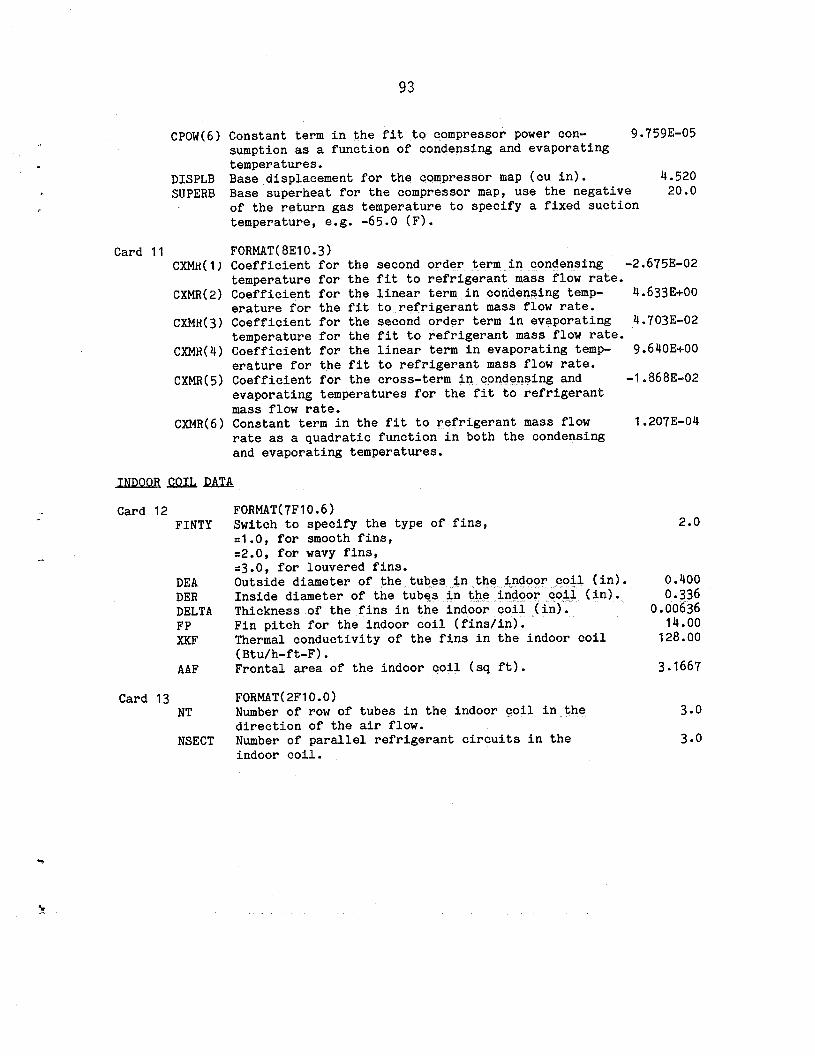
93
CPOW(6) Constant term in the fit to compressor power con- 9.7593-05 sumption as a function of condensing and evaporating temperatures.
DISPLB Base displacement for the compressor map (cu in). 4.520 SUPERB Base superheat for the compressor map, use the negative 20.0
of the return gas temperature to specify a fixed suction temperature, e.g. -65.0 (F).
Card 11 FORMAT(8E10.3) CXMR(1) Coefficient for the second order term in condensing -2.6753-02
temperature for the fit to refrigerant mass flow rate. CXMR(2) Coefficient for the linear term in condensing temp- 4.633E+00
erature for the fit to refrigerant mass flow rate. CXMH(3) Coefficient for the second order term in evaporating 4.7033-02
temperature for the fit to refrigerant mass flow rate. CXMR(4) Coefficient for the linear term in evaporating temp- 9.64OE+OO
erature for the fit to refrigerant mass flow rate. CXMR(5) Coefficient for the cross-term in condensing and -1.8683-02
evaporating temperatures for the fit to refrigerant mass flow rate.
CXMR(6) Constant term in the fit to refrigerant mass flow rate as a quadratic function in both the condensing and evaporating temperatures.
Card 12 FINTY
DEA DER DELTA FP XKF
AAF
Card 13 NT
NSECT
FORMAT(7F10.6) Switch to specify the type of fins, ~1.0, for smooth fins, ~2.0, for wavy fins, ~3.0, for louvered fins. Outside diameter of the tubes in the indoor coil (in). Inside diameter of the tubes in the indoor c?oil (in>.- Thickness of the fins in the indoor coil (in). Fin pitch for the indoor coil (fins/in). Thermal conductivity of the fins in the indoor coil (Btu/h-ft-F). Frontal area of the indoor coil (sq ft).
FORMAT(2FlO.O) Number of row of tubes in the indoor coil in the direction of the air flow. Number of parallel refrigerant circuits in the indoor coil.
1.2073-04
2.0
0.400 0.336
0.00636 14.00
128.00
3.1667
3.0
3.0

94
Card 14 FORMAT(3F10.5) HCONT Contact conductance between fins and tubes for
the indoor coil (Btu/h-sq ft-F). ST The vertical spacing of tube passes (in). WT The spacing of tube rows in the direction of air
flow (in).
Card 15 FORMAT(5F10.4) QA Air flow rate for the indoor coil (cfm). TAI Inlet air temperature for the indoor coil (F). RH Relative humidity of the inlet air for the indoor
coil. RTB The number of return bends in the indoor coil. FANEF Combined fan and fan motor efficiency for the indoor
coil.
Card 16 FINTY
DEA DER DELTA FP XKF
AAF
Card 17 NT
NSECT
Card 18 HCONT
ST
WT
Card 19 QA TAI RH
RTB FANEF
FORMAT(7F10.6) Switch to specify the type of fins, ~1.0, for smooth fins, ~2.0, for wavy fins, ~3.0, for louvered fins. Outside diameter of tubes in the outdoor coil (in). Inside diameter of the tubes in the outdoor coil (in). The thickness of the fins in the outdoor coil (in). The fin pitch for the outdoor coil (fins/in). The thermal conductivity of the fins in the outdoor coil (Btu/h-ft-F). The frontal area of the outdoor coil (sq ft).
FORMAT(2FlO.O) The number of rows of tubes in the outdoor coil in the direction of air flow. The number of parallel refrigerant circuits in the outdoor coil.
FORMAT(3F10.5) The contact conductance between the fins and tubes for the outdoor coil (Btu/h-sq ft-F). The vertical spacing of tube passes for the outdoor coil (in). The spacing of tube rows in the direction of air flow for the outdoor coil (in).
FORMAT(5F10.5) The air flow rate for the outdoor coil (cfm). The inlet air temperature for the outdoor coil (F). The relative humidity of the air entering the outdoor coil. The number of return bends in the outdoor coil. The combined fan and fan motor efficiency for the outdoor coil, not used if MFANFT=l on Card 3.
30000.0
1.00 0.875
1200.0 70.0 0.50
72.00 0.200
2.0
0.400 0.336
0.00636 14.00
128.00
5.040
3.0
4.0
30000.0
1 .oo
0.875
2300.0 47.0 0.70
64.00 0.160

95
Appendix B: Sample Input and Output Data
*
f
.5
SAMPLE DATA SET FOR ORNL HEAT PUMP DESIGN MODEL -- @ 47.OF AMBIENT 15000.0 8.00 10.00
2 1 1 2 1 0
o.,,o: 30.40 45.0 2000.00 300.00 200.00 0.6800 6.00 0.5550 30.40 0.6800 2.00 0.5550 2.00
30.00 130.00 400.0 2 4.520 3450.00 0.350
-1.5093-04 4.0893-02-1.3383-04 5.86OE% 3.6383-04 9.7593-05 4.523+00 2O.OE+OO -2.6753-02 4.6333+00 4.703E-02 9.6403+00-1.8683-02 1.207E-04
3.z 0.4000 3.000 0.3360 0.00636 14.0 128.0 3.1667
30000.00 1.00 0.875 1200.0 70.0 0.500 72.00 0.200
3.;;: 0.4000 4.000 0.3360 0.00636 14.0 128.0 5.0400
30000.00 1.0 0.875 2300.0 47.00 0.700 64.00 0.160
l **** INPUT DATA l ****
L
SAMPLE DATA SET FOR ORNL HEAT PUMP DESIGN MODEL -- @ 47.OF AMBIENT HEATING MODE OF OPERATION (NCORHz2)
THE HOUSE LOAD IS 15000. BTU/H DIAMETER OF 6 EQUIVALENT DUCTS- 8.000 IN COMPRESSOR CAN HEAT LOSS ADDED TO AIR BEFORE CROSSING THE OUTDOOR COIL. POWER TO THE INDOOR FAN ADDED TO AIR AFTER CROSSING THE COIL. POWER TO THE OUTDOOR FAN ADDED TO AIR BEFORE CROSSING THE COIL. CONDENSER SUBCOOLING IS HELD FIXED AT 45.00 F EVAPORATOR SUPERHEAT IS HELD FIXED AT 10.00 F
DESCRIPTION OF CONNECTING TUBING: LIQUID LINE FROM INDOOR TO OUTDOOR HEAT EXCHANGER
ID 0.19000 IN EQUIVALENT LENGTH 30.40 FT
FROM INDOOR COIL TO REVERSING VALVE FROM OUTDOOR COIL TO REVERSING VALVE ID 0.55500 IN ID 0.68000 IN EQUIVALENT LENGTH 30.40 FT EQUIVALENT LENGTH 6.00 FT
FROM REVERSING VALVE TO COMPRESSOR INLET FROM REVERSING VALVE TO COMPRESSOR OUTLET ID 0.68000 IN ID 0.55500 IN EQUIVALENT LENGTH 2.00 FT EQUIVALENT LENGTH 2.00 FT
HEAT LOSS IN DISCHARGE LINE 2000.0 BTU/H HEAT GAIN IN SUCTION LINE 300.0 BTU/H HEAT LOSS IN LIQUID LINE 200.0 BTU/H
ESTIMATE OF: REFRIGERANT MASS FLOW RATE 400.000 LBM/H SATURATION TEMPERATURE INTO CONDENSER 130.000 F SATURATION TEMPERATURE OUT OF EVAPORATOR 30.000 F
COMPRESSOR CHARACTERISTICS: TOTAL DISPLACEMENT 4.520 CUBIC INCHES SYNCHRONOUS MOTOR SPEED 3450.000 RPMS
MAP-BASED COMPRESSOR INPUT: POWER CONSUMPTION. -1.509%04*CONDENSING TEMPERATURE**2 + 4.089E-02'CONDENSING TEMPERATURE
+ -1.338E-04'EVAPORATING TEMPERATURE**2 + 5.860E-04*EVAPORATING TEMPERATURE + 3.638E-04'CONDENSING TEMPERATURE*EVAPORATING TEMPERATURE,+ 9;i59E:05
MASS FLOW RATE- -2.675E-02*CONDENSING TEMPERATURE**2 + 4.633E+OO*CONDENSING TEMPERATURE + 4.703E-02*EVAPORATING TEMPERATURE**2 + 9.640E+OO*EVAPORATING TEMPERATURE + -1.868E-02*CONDENSING TEMPERATURE*EVAPORATING TEMPERATURE + 1.2073-04
CORRECTION FACTOR FOR SUCTION GAS 0.330 CORRECTION FACTOR FOR VOLUMETRIC EFFICIENCY 0.750 BASE SUPERHEAT FOR COMPRESSOR MAP 20.000 F BASE DISPLACEMENT FOR COMPRESSOR MAP 4.520 CU IN
HEAT REJECTED FROM COMPRESSOR SHELL IS 0.35 TIMES THE COMPRESSOR POWER

INDOOR UNIT: CONDENSER OD OF TUBES IN HX 0.40000 IN ID OF TUBES IN HX 0.33600 IN FRONTAL AREA OF HX 3.167 SQ FT NUMBER OF PARALLEL CIRCUITS 3.00 NUMBER OF TUBES IN DIRECTION OF AIR FLOU 3.00 NUMBER OF RETURN BKNDS 72.00 AIR PLOW RATE 1200.00 CFM INLET AIR TEMPERATURE 70.000 F WAVY FINS
OUTDOOR UNIT: EVAPORATOR OD OF TUBES IN HX 0.40000 IN ID OF TUBES IN HX 0.33600 IN FRONTAL AREA OF HX 5.040 SQ FT NUMBER OF PARALLEL CIRCUITS 4.00 NUMBER OF TUBES IN DIRECTION OF AIR FLOW 3.00 NUMBER OF RETURN BENDS 64.00 AIR FLOW RATE 2300.00 CFM ISLET AIR TKMPERATURE 47.000 F WAVY FINS
FIN THICKNESS FIN PITCH THERMAL CONDUCTIVITY OF FINS CONTACT CONDUCTANCE HORIZONTAL TUBE SPACING VERTICAL TUBE SPACING FAN BFFICIENCY RELATIVE HUMIDITY
FIN THICKNESS FIN PITCH THERMAL CONDUCTIVITY OF FINS CONTACT CONDUCTANCE HORIZONTAL TUBE SPACING VERTICAL TUBE SPACING FAN EFFICIENCY RELATIVE HUMIDITY
0.00636 IN 14.00 FINS/IN
128.000 BTU/H-FT-F 30000.0 BTU/H-SQ FT-F
0.875 IK 1.000 IN
0.20000 0.50000
0.00636 IN 14.00 FINS/IN
128.000 BTU/H-FT-F 30000.0 BTU/H-SQ FT-F
0.875 IN 1.000 IN
0.16000 0.70000

i ; ’ I
l **** CALCULATED HEAT PUMP PERFORMANCE *****
COMPRESSOR OPERATING CONDITIONS: EFFICIENCY
COMPRESSOR PGWER 4.011 Km VOLUMETRIC 0.6311 MOTOR SPEED 3450.000 RPH OVERALL 0.5053
REFRIGERANT MASS FLOW RATE 413.828 LBWH POWER PER UNIT MASS FLOW COMPRESSOR SHELL HEAT LOSS 4791.414 BTU/H POWER CORRECTION FACTOR
33;3;9";; BTlJ/LBM
MASS FLOW RATE CORRECTION FACTOR 1:0089
REFRIGERANT SATURATION TEMPERATURE TEMPERATURE
INLET 39.470 F 29.577 F 43.687 29.263
206.498 126.899
REFRIGERANT ENTHALPY
108.958 BTU/LBM
REFRIGERANT QUALITY
1 .oooo 1.0000 1.0000
1 .oooo 0.0
REFRIGERANT PRESSURE
SYSTEM SUMMARY
COMPRESSOR SUCTION LINE SHELL INLET SHELL OUTLET
109.683 131.185
CONDENSER INLET 183.889 F 126.558 F 126.352 BTU/LB!4 OUTLET 81.217 126.196 33.477
AIR TEMPERATURE
70.000 F 100.147
47.000 F 38.908
69.054 PSlA 68.660
299.682
120.765 F
34.916 F 29.577
298.411 PSIA 297.060
277.316 PSIA
'V$E~ PSlA .
79.607 F
34.916 F 39.470
32.994 BTU/LBM 0.0
32.994 BTU/LBM 0.1483 108.958 1.0000
EXPANSION DEVICE
EVAPORATOR INLET OUTLET
PERFORMANCE OF EACH CIRCUIT IN THE CONDENSER INLET AIR TEMPERATURE 70.000 F OUTLET AIR TEMPERATURE 100.147 F
HEAT LOSS FROM FAN 1257.1 BTU/H AIR TEMPERATURE CROSSING COIL 99.193 F
TOTAL SEAT EXCHANGER EFFECTIVENESS 0.6949
SUPERHBATER TWO-PHASE suBcooLED REGION REGION RRGION
NTU 0.0 1.1351 1.9987 HEAT EXCHANGER EFFECTIVENESS 1.0000 0.6786 0.8005 CR/CA 0.0 0.2816 FRACTION OF HEAT EXCHANGER 0.0 0.6453 0.3547 HEAT TRANSFER RATE 0.0 BTU/H 10838.4 BTU/H 1973.0 BTU/H OUTLET AIR TEHPERATURE 70.000 9 108.270 F 82.676 F
W U
AIR SIDE: REFRIGERANT SIDE: MASS FLOW RATE 1798.1 LBH/H MASS FLOW RATE 137.9 LBWH PRESSURE DROP HBAT TRAESFER
COEFFICIENT
0.5224 IN H20 PRESSURE ,DROP 1.351 PSI HEAT TRANSFER CORFFICIENT
13.136 BTU/H-SQ FT-F VAPOR REGION TWO PHASE REGION SUSCOOLBD REGION
102.905 BTU/H-SQ FT-F 453.291 BTU/B-Sp FT-F 110.787 BTU/H-SQ PT-F
TV0 PBASE REGION (BTU/B-P) SUB~OGLED REGION (BTU/H-F) REFRIGERANT SIDE 2933.419 REFRIGERANT SIDE 394.035 AIR SIDE 1436.706 AIR SIDE 789.615 COKBINED 964.380 COMBINED 262.862
UA VALUES: VAPOR REGION (BTU/H-F)
REFRIGERANT SIDE 0.0 AIR SIDE 0.0 conB1NED 0.0

n .ow CONTROL DRVICE - CONDENSER SUBCOOLING IS SPECIFIED AS 45.000 F CORRESPONDING TXV RATING PARAMRTERS: CORRESPONDING CAPILLARY TUBE PARAMETERS:
RATRD OPERATING SUPERHEAT 11.000 F NUMBER OF CAPILLARY TUBES 1 STATIC SUPERHEAT RATING 6.000 F CAPILLARY TUBE FLOW FACTOR 2.626 PERMANENT BLEED FACTOR 1.150 TXV CAPACITY RATING 1.880 TONS
INCLUDING NOZZLE AND TUBES
CORRESPONDING ORIFICE PARAMRTER: ORIFICE DIAHETER 0.0544 IN
PERFORMANCE OF EACH CIRCUIT IN THE EVAPORATOR INLET AIR TEMPERATURE 47.000 F
HEAT LOSS FROM COMPRESSOR 4791.4 BTU/H HEAT LOSS FROM FAN 2274.5 BTU/H AIR TEMPERATURE CROSSING COIL 49.696 F
OUTLET AIR TEMPERATURE 38.908 F
MOISTURE REMOVAL OCCURS
SUNMARY OF DEHUMYDIFICATION PERFORMANCE (TWO-PHASE REGION)
LEADING EDGE POINT WHERE MOISTURE OF COIL REMOVAL BEGINS LEAVING EDGE OF COIL
AIR AIR WALL AIR WALL DRY BULB TEMPERATURE 49.696 F 44.912 F 37.740 F 38.400 F F HUMIDITY RATIO 0.00475
35.434 0.00475 0.00475 0.00446 0.00433
ENTHALPY 17.090 BTU/LBH 15.930 BTU/LBM 14.191 BTU/LB!+! 14.036 BTU/LBM 13.183 BTU/LBM
RATE OF MOISTURE REMOVAL 0.7345 LBM/H FRACTION OF NAPORATOR THAT IS WET 0.6941 LATENT HEAT TRANSFER RATE IN TWO-PHASE REGION 789. BTU/H SENSIBLE HEAT TRANSFER RATE IN TWO-PHASE REGION 6896. BTU/H SENSIBLE TO TOTAL HEAT TRANSFER RATIO FOR TWO-PHASE REGION 0.8974
OVERALL SENSIBLE TO TOTAL HEAT TRANSFER RATIO 0.8996
OVERALL CONDITIONS ACROSS COIL ENTERING EXITING
AIR AIR DRY BULB TEMPERATURE 49.696 F 38.908 F WET BULB TMPERATURE 43.924 F 37.659 F RELATIVE HUMIDITY 0.633 0.901 HUMIDITY RATIO 0.00475 0.00448
TOTAL HEAT EXCHANGER EFFECTIVENESS (SENSIBLE)
SUPERHEATED REGION
NTU 0.7608 HEAT EXCHANGER EFFECTIVENESS 0.4834 CR/CA 0.4025 FRACTION OF HEAT EXCHANGER 0.0682 HEAT TRANSFER RATE 172.2 BTU/H ,-.- ~~ _~~ AIR MASS FLOW RATE 184.36 LBM/H OUTLET AIR TEMPERATURE 45.845 F
AIR SIDE MASS FLOW RATE 2702.1 LBM/H PRESSURE DROP 0.395 IN HZ0 HEAT TRANSFER COEFFICIENT
0.6476
TWO-PHASE REGION 1.0590 0.6532
0.9318 7684.9 BTU/H
2517.70 LBM/H 38.400 F
REFRIGERANT SIDE MASS FLOW RATE 103.5 LBM/H PRESSURE DROP 7.005 PSI HEAT TRANSFER COEFFICIENT ,- - DRY COIL 14.462 BTU/H-SQ FT-F VAPOR REGION 63.625 BTU/H&Q Fr-r
WET COIL 16.803 BTU/H-SQ FT-F TN0 PHASE REGION 631.979 BTU/H-S9 FT-F
DRY FIN EFFICIENCY 0.791 WET FIN EFFICIENCY 0.763

UA VALUES: VAPOR TWO PHASE REGION REGION
REFRIGERANT SIDE 69.286 9398.352 BTU/H-F AIR SIDE
DRY COIL 261.250 1091.526 BTU/H-F WET COIL 2772.596 BTU/H-F
COMBINED DRY COIL 54.763 791.186 BTU/H-F WET COIL 1945.610 BTU/H-F
SUMMARY OF ENERGY INPUT AND OUTPUT: SAMPLE DATA SET FOR ORNL HEAT PUMP DESIGN MODEL -- @ 47.0F AMBIENT AIR TBMPERATURE INTO EVAPORATOR 47.00 F HEAT FROM CONDENSER TO AIR 38434. BTU/H HEAT TO EVAPORATOR FROM AIR 71428. BTU/H POWER TO INDOOR FAN -1257. BTU/H POWER TO OUTDOOR FAN 2275. BTU/H POWER TO COMPRESSOR MOTOR 13690. BTU/H COMPRESSOR SHELL HEAT LOSS 4791. BTU/H TOTAL HEAT TO/FROM INDOOR AIR 39691. BTU/H
SYSTEM EFFICIENCY: cop (HEATING) COP (WITH RESISTANCE HEAT)
HEAT OUTPUT: 2.305 HEAT FROM HEAT PUMP 39691.29 BTU/H 2.305 RESISTANCE HEAT 0.0 BTU/H
HOUSE LOAD 15000.00 BTU/H


101
Appendix C - Definitions of Constants Assigned in BLOCK DATA Subroutine
A number of variables and constants are used by the Heat Pump
Design Model that are unlikely to be changed very often, and conse-
quently they are simply assigned values rather than being specified with
each set of input data. They have been brought together in the BLOCK
DATA subroutine and given values which are in turn passed to the sub-
routines where they are used via common blocks. These data are divided
into several categories determined by-use; they are defined in that
"natural" order.
Physical Air-Side Parameters
AFILTR cross-sectional area of filter on indoor unit, 2.78 ft*
AHEATR cross-sectional area of resistance heaters in indoor unit, 1.28 ft*
PA atmospheric pressure, 14.7 lbf/in*
RACKS number of resistance heater racks, 3.0
RAU universial gas constant, 53.34 ft-lbf/lbm-OR
Refrigerant Tubing Parameter
E roughness of interior tube walls, 5 x low6 ft
Compressor Motor Efficiency
CETAM coefficients for the 0th through 5th order terms of the fit of the compressor motor efficiency as a function of the fractional motor load (Eq. 4.29), 0.4088, 2.5138, -4.6289, 4.5884, -2.3666, and 0.48324
RPMSLR slope of linear fit for fraction of no-load compressor motor speed as a function of fraction of full load power, -0.042 (see Eq. 4.24)

102
Data for Outdoor Fan Efficiency --
COFAN constant term for the fit of outdoor fan static efficiency to . fan specific speed, -3.993
.
ClFAN coefficient for the linear term of the fit of outdoor fan .
static efficiency to the fan specific speed, 4.266
C2FAN coefficient for the quadratic term of the fit of outdoor fan static efficiency to fan specific speed, -1.024
EFFMOT constant motor efficiency for the outdoor fan, 0.55
RPMFAN constant motor speed for the outdoor fan, 825 rpm
Tolerance Parameters
AMBCON
CMPCON
CNDCON
CONMST
EVPCON
FLOCON
TOLH
TOLS
convergence parameter for the outdoor ambient air interation, 0.20 F".
convergence parameter for the Ah iteration in the compressor calculations, 0.05 Btu/lbm
convergence parameter for iterations on condenser subcooling and refrigerant temperature at the flow control device, 0.20 0.20 F"
tolerance parameter for the iterations on evaporator tube wall temperatures, 0.003 F"
tolerance parameter for iterations on evaporator superheat, 0.5O"F.
convergence criteria for iterations on refrigerant mass flow rate through the expansion device, 0.2 lbm/h
tolerance parameter used in calculating properties of super- heated vapor when enthalpy is known, 10e3
tolerance parameter used in calculating properties of super- heated vapor when entropy is known, 10 4
Refrigerant Specification
NR refrigerant number, 22
Refrigerant-Side Heat Transfer Correlation for Single-Phase Regions .^
ClR, C3R, and C5R coefficients for single-phase heat transfer coefficient (Eq. 6.2), 1.10647, 3.5194 x 10m7, and 0.01080

103
I CZR, C4R, and C6R exponents for single-phase heat transfer coefficient (Eq. 6.3), -0.78992, 1.03804, and -0.13750
-.
. I
ULR
XLLR
lower limit for the Reynolds number for turbulent flow of refrigerant, 6,000
upper limit on the Reynolds number for laminar flow of refriger- ant, 3,500
Thermostatic Expansion Valve Constants
BLEEDF
DPRAT
NZTBOP
STATIC
SUPRAT
f TERAT
TLQRAT
bypass or bleed factor coefficient used to compute TXV para- meters when condenser subcooling is held fixed, 1.15
rated pressure drop across the TXV at the design conditions, 100 psi for R-22 and R-502, 50 psi for R-12
switch to bypass nozzle and distributor tube pressure drop calculations when calculating TXV parameters if the condenser subcooling is held fixed, 0
static superheat setting used to compute the TXV parameters when the condenser subcooling is held fixed, 6.0 F”
rated operating superheat used to compute the TXV parameters when the condenser subcooling is held fixed, 1l.O.F"
rated evaporating temperature for the TXV, 4O.O"F
rated liquid refrigerant temperature at the inlet to the TXV, lOO.O"F
Capillary Tube Parameter
NCAP number of capillary tubes used to compute capillary tube flow factor, $, when condenser subcooling is held fixed, 1
Compressor Efficiency Parameters
ETAVLA intercept of the fit of theoretical minus actual compressor volumetric efficiencies as a linear function of the correlating parameter of Davis and Scott, -0.0933
ETAVLB slope of the fit of theoretical minus actual compressor volumetric efficiencies as a linear function of the correlating parameter of Davis and Scott, 0.733
SUCFAC suction gas heating factor Fsh used in Eq. 4.6, 0.33
VOLFAC volumetric efficiency correction factor Fv used in Eq. 4.4, 0.75


105
Appendix D: Definitions of Variables in Common Blocks
Variable Definition A constant used in a first order approximation of the
saturation temperature in the logarithm of the refrigerant pressure. assigned a value in TABLES and used in TSAT.
AAFC the frontal area of the condenser, read by DATAIN, used by CALC and COND (sq ft).
AAFE the frontal area of the evaporator, read by DATAIN, used by CALC and EVAPR (sq ft).
ACV,BCV,..., FCV constants used in calculating refrigerant heat capacity with temperature and specific volume, assigned values in TABLES and used in SATPRP.
AFILTR frontal area of filter for the indoor unit, assigned a value in BLOCK DATA and used in PDAIR (sq ft).
AHEATR cross-sectional area of the resistance heaters, assigned a value in BLOCK DATA and used in PDAIR (sq ft).
AL.BL,...,GL coefficients for expressing density of the liquid
ALFAAC
AALFE
ALFARC
ALFARE
ALPHA
AMBCON
ARFTC
refrigerant as a function of absolute temperature (R), assigned values in TABLES and used in SATPRP (lbm/cu ft).
ration of the air-side heat transfer area for the condenser to the total volume of the condenser, calculated in CALC, used by COND, EFFCT, and EXCH (/ft).
ratio of the air-side heat transfer area for the evaporator to the total volume of the evaporator, calculated in CALC, used by EVAP and EVAPR (/ft).
ratio of the total refrigerant-side heat transfer area for the condenser to the volume of the condenser, calculated in CALC, used by COND, EFFCT, and EXCH (/ft).
ratio of the total refrigerant side heat transfer area for the evaporator to the volume of the evaporator, calculated in CALC, used by EVAP and EVAPR (/ft).
constant used in refrigerant equation of state correlating pressure with temperature and specific volume, assigned a value in TABLES, used by SATPRP, SPVOL, and VAPOR.
tolerance parameter for the ambient air temperature iteration in the main program, assigned a value in BLOCK DATA and used in the main program (F).
inside cross-sectional area of the tubes in the condenser calculated in CALC and used in COND (ft).
Common SUPER
CONDEN
EVAPOR
OTHER
AIR
AIR
DENSIT
CONDEN
EVAPOR
CONDEN
EVAPOR
STATEQ
MPASS
CONDEN

, 106
ARFTE inside cross-sectional area of the tubes in the evaporator calculated in CALC and used by EVAPR (sq ft).
ARHTC total refrigerant-side heat transfer area for each circuit in the condenser, calculated and used in CALC, used by COND, EFFCT, and EXCH (sq ft).
ARHTC total refrigerant side heat transfer area for each circuit in the evaporator, calculated and used in CALC, used by EVAP and EVAPR (sq ft).
AVP,BVP,..., FVP constants used in correlating refrigerant vapor pressure with absolute temperature (R), assigned values in TABLES, used in SATPRP and TSAT.
A2,B2,C2 constants used in refrigerant equations of state correlating pressure with temperature and specific volume, assigned values in TABLES, used by SATPRP, SPVOL, and VAPOR.
A3,B3,C3 constants used in refrigerant equations of state correlating pressure with temperature and specific volume, assigned values in TABLES, used by SATPRP, SPVOL, and VAPOR.
A4,B4,C4 constants used in refrigerant equations of state correlating pressure with temperature and specific volume, assigned values in TABLES, used by SATPRP, SPVOL, and VAPOR.
A5,B5,C5 constants used in refrigerant equations of state correlating pressure with temperature and specific volume, assigned values in TABLES, used by SATPRP, SPVOL, and VAPOR.
A6,B6,C6 constants used in refrigerant equations of state correlating pressure with temperature and specific volume, assigned values in TABLES, used by SATPRP, SPVOL, and VAPOR.
B
BLEEDF
Bl
constant used in a first order approximation to the refrigerant saturation temperature as a function of the logarithm of the saturation pressure, assigned value in TABLES and used in TSAT.
by-pass or bleed factor coefficient for the thermostatic expansion valve, assigned a value by BLOCK DATA or read by DATAIN, used by TXV.
constant used in refrigerant equation of state correlating pressure with temperature and specific volume, assigned a value in TABLES, used by SATPRP, SPVOL, and VAPOR.
EVAPOR
CONDEN * c
EVAPOR
SAT
STATEQ
STATEQ
STATEQ 1
STATEQ _
STATEQ
SUPER
TXVDAT
STATEQ

CA
c CANFAC
.
CAP
CAPFLO
CAPNOZ
CAPTUB
CARC
CARE 2.
CETAM
CLCXMR
CMPCON
CNDCON
‘
COIL II
107
air-side heat capacity rate for the superheated portion of the EFFARG of the condenser, calculated in EFFCT, used by EXCH (Btu/h-F).
factor used to express compressor shell heat rejection as a fraction of compressor power consumption, read by DATAIN end used by COMP.
COMPR
capacity of the evaporator at the operating conditions TXVDAT with an assumed 10 F of superheat at the evaporator exit, calculated in and used in TXV, printed by OUTPUT (Btu/hr),
capillary tube flow factor, default value assigned in BLOCK FLOWBA DATA, read by DATAIN if capillary tube submodel is used, calculated or used by CAPTUB, printed by OUTPUT.
heating capacity of the nozzle of the thermostatic expansion TXVDAT valve, calculated and used in TXV, printed by OUTPUT (Btu/hr).
heating capacity of each tube from the thermostatic expansion valve to the evaporator, calculated and used in TXV, printed in OUTPUT (Btu/hr).
ratio of the fin heat transfer area to the contact area between the fins and the tubes in the condenser, calculated in CALC and used in COND.
ratio of the fin heat transfer. area to the contact area between the fins and the tubes in the evaporator, calculated in CALC and used by EVAP.
coefficients for a fit to the motor efficiency as a function of the fraction of full load power output, assigned values in BLOCK DATA and used by COMP.
refrigerant mass flow rate through each capillary tube, calculated in CAPTUB, used by FLOBAL, and printed in OUTPUT (lbm/hr).
tolerance parameter for the iteration on the enthalpy entering the compressor suction port in COMP, assigned a value in BLOCK DATA (Btu/h-F).
tolerance parameter for the condenser subcooling iterations in the main program and in COND, and the refrigerant temperature at the flow control device in FLOBAL, assigned a value in BLOCK DATA, used in the main program, COND, and FLOBAL (F).
evaporator coil resistance to heat transfer, calculated and used in EVAP, used by TWISOL.
TXVDAT
CONDEN
EVAPOR
CMPMOT
PRNT2
MPASS
MPASS
TWI
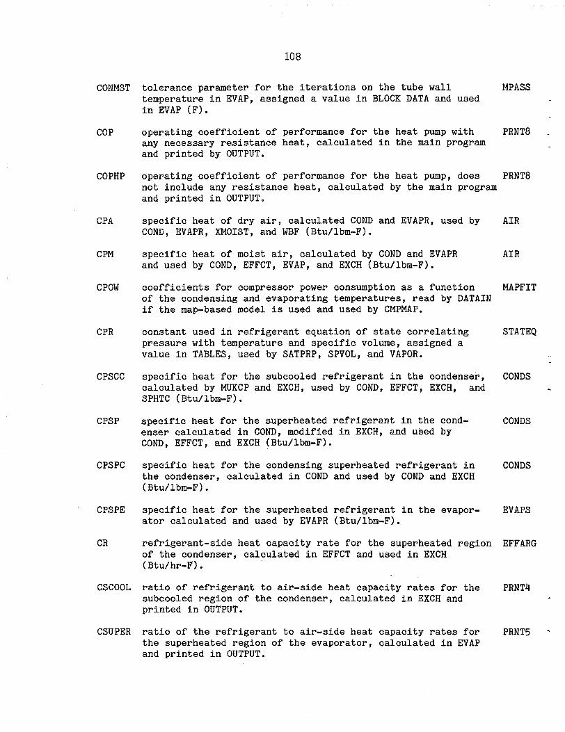
108
CONMST
COP
COPHP
CPA
CPM
CPOW
CPR
CPSCC
CPSP
CPSPC
CPSPE
CR
CSCOOL
CSUPER
tolerance parameter for the iterations on the tube wall MPASS temperature in EVAP, assigned a value in BLOCK DATA and used in EVAP (F).
operating coefficient of performance for the heat pump with PRNT8 any necessary resistance heat, calculated in the main program and printed by OUTPUT.
operating coefficient of performance for the heat pump, does PRNT8 not include any resistance heat, calculated by the main program and printed in-OUTPUT.
specific heat of dry air, calculated COND and EVAPR, used by COND, EVAPR, XMOIST, and WBF (Btu/lbm-F).
specific heat of moist air, calculated by COND and EVAPR and used by COND, EFFCT, EVAP, and EXCH (Btu/lbm-F).
coefficients for compressor power consumption as a function of the condensing and evaporating temperatures, read by DATAIN if the map-based model is used and used by CMPMAP.
constant used in refrigerant equation of state correlating pressure with temperature and specific volume, assigned a value in TABLES, used by SATPRP, SPVOL, and VAPOR.
specific heat for the subcooled refrigerant in the condenser, calculated by MUKCP and EXCH, used by COND, EFFCT, EXCH, and SPHTC (Btu/lbm-F).
specific heat for the superheated refrigerant in the cond- enser calculated in COND, modified in EXCH, and used by COND, EFFCT, and EXCH (Btu/lbm-F).
specific heat for the condensing superheated refrigerant in the condenser, calculated in COND and used by COND and EXCH (Btu/lbm-F).
specific heat for the superheated refrigerant in the evapor- ator calculated and used by EVAPR (Btu/lbm-F).
refrigerant-side heat capacity rate for the superheated region of the condenser, calculated in EFFCT and used in EXCH (Btu/hr-F).
ratio of refrigerant to air-side heat capacity rates for the subcooled region of the condenser, calculated in EXCH and printed in OUTPUT.
ratio of the refrigerant to air-side heat capacity rates for the superheated region of the evaporator, calculated in EVAP and printed in OUTPUT.
AIR
AIR
MAPFIT
STATEQ
CONDS
CONDS
CONDS
EVAPS
EFFARG
PRNT4 e
PRNT5 *

. CUASCA
CUASC
CUASCR
CUATP
CUATPA
CUATPR
CUAV
CUAVA
CUAVR
CXMR
109
overall thermal conductance times the heat transfer area (UA) for the subcooled region of the condenser, calculated in COND and printed in OUTPUT (Btu/hr-F).
air-side thermal conductance times the heat transfer area (UA) for the subcooled region of the condenser, calculated in COND and printed in OUTPUT (Btu/hr-F).
refrigerant-side thermal conductance times the heat transfer area (UA) for the subcooled region of the condenser, calc- ulated in COND and printed in OUTPUT (Btu/hr-F).
overall thermal conductance times heat transfer area (UA) for the two-phase region of the condenser, calculated in COND and printed in OUTPUT (Btu/hr-F).
air-side thermal conductance times the heat transfer area (UA) for the two-phase region of the condenser, calculated in COND and printed in OUTPUT (Btu/hr-F).
refrigerant-side thermal conductance times the heat transfer area (UA) for the two-phase region of the condenser, calcuated in COND and printed in OUTPUT (Btu/hr-F).
overall thermal conductance times the heat transfer area for the vapor region of the condenser, calculated in COND and printed in OUTPUT (Btu/hr-F).
air-side thermal conductance times the heat transfer area (UA) for the vapor region of the condenser, calculated in COND and printed in OUTPUT (Btu/hr-F).
refrigerant-side thermal conductance times heat transfer area for the superheated region of the condenser, calculated in COND and printed in OUTPUT (Btu/hr-F).
coefficients for the refrigerant mass flow rate as a function of the condensing and evaporating temperatures, read by DATAIN, if the map-based compressor model is chosen, and used by CMPMAP.
COFAN,ClFAN,C2FAN coefficients for the fan static efficiency for the outdoor heat exchanger as a function of the static speed of the fan, assigned values in BLOCK DATA and used by FANFIT.
ClR,C2R ,...,C6R coefficients and exponents for fit to single-phase heat transfer coefficient as a function of refrigerant Reynolds and Prandtl numbers, assigned values in BLOCK DATA and used in SPHTC.
UAS
UAS
UAS
UAS
UAS
UAS
UAS
UAS
UAS
MAPFIT
FANMOT
VAPHTC

/
110
DDL
DDLRV
DDUCT
DEAC
DEAE
DELTAC
DELTAE
DERC
DERE
DISPL
DLL
DP
DPDL
DPLL
DPNOZ
DPRAT
inside diameter of the compressor discharge line from the reversing valve to the condenser, assigned a value by DATAIN and used by COMP (ft).
inside diameter of the line from the compressor discharge port to the reversing valve, read by DATAIN and used by COMP (ft).
diameter of each of 6 identical air ducts with equivalent lengths of 100 ft, read by DATAIN and used by COND and EVAPR (ft).
outside diameter of the tubes in the condenser, read by DATAIN, used by CALC and COND (ft).
outside diameter of the tubes in the evaporator, read by DATAIN, used by CALC, EVAP and EVAPR (ft).
thickness of the fins in the condenser, read by DATAIN, used by CALC and COND (ft).
thickness of the fins in the evaporator, read by DATAIN, used by CALC and EVAPR (ft).
inside diameter of the refrigerant tubes in the condenser, read by DATAIN, used by CALC and COND (ft).
inside diameter of the refrigerant tubes in the evaporator, read by DATAIN, used by CALC and EVAPR (ft).
total compressor piston displacement, read by DATAIN and used by COMP (cu in).
inside diameter of the liquid line connecting the indoor and outdoor heat exchangers, read by DATAIN and used by FLOBAL (ft).
air-side pressure drop across the outdoor coil, calculated in FANFIT and printed by OUTPUT (inches of water).
pressure drop in the compressor discharge line from the discharge port to the condenser, calculated and used by COMP (psi).
pressure drop in the liquid line connecting the heat exchangers, calculated and used in FLOBAL (psi).
LINES
.
LINES -
BLANK
CONDEN
EVAPOR
CONDEN
EVAPOR
CONDEN .
EVAPOR *
COMPR
LINES
PRNTS
LINES
LINES
pressure drop in the nozzle for the thermostatic expansion TXVDAT - valve, calculated and used in TXV, print in OUTPUT (psi).
rated pressure drop across the thermostatic expansion valve TXVDAT * at the design conditions, assigned a value in BLOCK DATA and used by TXV (psi).

111
DPSL
DPTUBE
DPTXV
DSL
DSLRV
DTROC
DZC
DZE h s
E
EFFMMX
EFFMOT
EINDF
EOUTF
ETAISN
pressure drop in the suction line connecting the evaporator and compressor, calculated and used in COMP (psi).
pressure drop across the tubes from the thermostatic expan- sion valve to the evaporator, calculated and used in TXV, printed in OUTPUT (psi).
pressure drop across the valve of the thermostatic expansion valve (does not include nozzle and tube losses), calculated and used in TXV, printed in OUTPUT (psi).
inside diameter of the suction line from the evaporator to the reversing valve, read by DATAIN and used by COMP (ft).
inside diameter of the line from the compressor suction port to the reversing valve, read by DATAIN and used by COMP (ft).
specified condenser subcooling, read by DATAIN used by CNDNSR, FLOBAL, and FLODEV, and printed by OUTPUT (F).
equivalent length of the refrigerant tubing in the condenser, calculated in CALC and used by COND.
LINES
TXVDAT
TXVDAT
LINES
LINES
FLOWBA
CCNDEN
equivalent length of the refrigerant tubing in the evaporator, EVAPOR calculated in CALC and used by EVAPR.
roughness factor for all of the refrigerant lines, assigned a value in BLOCK DATA, used by COMP, COND, EVAPR, and FLOBAL (ft).
product of the maximum motor efficiency and the mechanical efficiency for the compressor, read by DATAIN and used by COMP.
fan motor efficiency for the outdoor fan, assigned a value in BLOCK DATA and used in FANFIT.
rate of power consumption for the indoor fan, calculated in COND or EVAPR, used by the main program, printed by OUTPUT (Btu/hr).
rate of power consumption for the outdoor fan, calculated in COND or EVAPR, used by the main program, printed by OUTPUT (Btu/hr).
isentropic efficiency from the suction port to the discharge port of the compressor, read by DATAIN and used by COMP, printed and used by OUTPUT.
LINES
COMPR
FANMOT
PRNT8
PRNT8
COMPR

ETAMEC
ETAMOT
ETASUP
ETATOT
ETAVLA
ETAVLB
ETAVOL
ETP
ETPE
EUATP
EUATPA
EUATPR
EUAV
EUAVA
112
mechanical efficiency of the compressor, read by DATAIN and used by COMP.
operating motor efficiency for the PRNTlessor, calculated and used in COMP, used and printed by OUTPUT.
compressor suction gas heating efficiency, calculated by COMP and printed by OUTPUT.
compressor overall isentropic efficiency from the shell inlet to the shell outlet, calculated by COMP, used and printed by OUTPUT.
intercept of the fit of theoretical minus actual compressor volumetric efficiency as a linear function of the correlating parameter of Davis and Scott, assigned in BLOCK DATA and used in COMP.
slope of the fit of theoretical minus actual compressor volumetric efficiency as a linear function of the correlating parameter of Davis and Scott, assigned in BLOCK DATA and used in COMP.
volumetric efficiency of the compressor based on the shell inlet conditions, calculated and used in COMP, printed by OUTPUT.
heat exchanger effectiveness for the two-phase region of the condenser, calculated and used in EXCH, used and printed in OUTPUT.
heat exchanger effectiveness for the two-phase region of the evaporator, calculated and used in EVAP, printed by OUTPUT.
overall thermal conductance times heat transfer area (UA) for the two-phase region of the evaporator, calculated in EVAPR, printed in OUTPUT (Btu/hr-F).
COMPR i
COMPR - *
PRNTI
PRNTl
COMPR
COMPR
PRNTl L 1
PRNT4 -
PRNT5
UAS
air-side thermal conductance times the heat transfer area (UA) UAS for the two-phase region of the evaporator, calculated in EVAPR and printed in OUTPUT (Btu/hr-F).
refrigerant-side thermal conductance times the heat transfer UAS area (UA) for the two-phase region of the evaporator, calc- ulated in EVAPR and printed in OUTPUT (Btu/hr-F).
overall thermal conductance times the heat transfer area (UA) UAS for the superheated region of the evaporator, calculated in EVAPR and printed in OUTPUT (Btu/hr-F). .
air-side thermal conductance times the heat transfer area (UA) UAS for the superheated region of the evaporator, calculated in EVAPR and printed in OUTPUT (Btu/hr-F).

' EXFR
EXFRC
EXFRE
EXFS
EXFSC
FANEFC
FANEFE
FANOUT
FARC
FARE 3.
FINTYC
113
refrigerant-side thermal conductance times the heat transfer area (UA) for the superheated region of the evaporator, CalC- ulated in EVAPR and printed in OUTPUT (Btu/hr-F).
tolerance parameter for the iteration on evaporator superheat in the main program and in EVAPR, assigned a value in BLOCK DATA and used in the main program and EVAPR (F).
heat exchanger effectiveness for the subcooled region of the condenser based on effectiveness-NTU correlations for cross- flow heat exchangers, calculated and used in EXCH.
heat exchanger effectiveness for the subcooled region of the condenser, assigned a value in EXCH, used and printed in OUTPUT.
heat exchanger effectiveness for the superheated region of the evaporator, calculated and used in EVAP, printed by OUTPUT.
heat exchanger effectiveness for the superheated region of the condenser based on heat capacity rates and delta T's, calc- ulated in EFFCT and used by EXCH.
heat exchanger effectiveness for the superheated region of the condenser, assigned a value in EXCH, used and printed in OUTPUT.
the combined fan-fan motor efficiency for the condenser, the value is either read by DATAIN or calculated by FANFIT;used by COND.
the combined fan-fan motor efficiency for the evaporator, the value is either read by DATAIN or calculated by FANFIT, used by COND.
combined operating efficiency of the outdoor fan-fan motor, calculated in FANFIT, printed by OUTPUT.
ratio of the fin heat transfer area for the condenser to the total heat transfer area on the air side, calculated in CALC and used in COND.
ratio of the fin heat transfer area for the evaporator to the total heat transfer area, calculated in CALC, used by EVAP and EVAPR.
switch to specify the type of fins in the condenser (smooth, wavy, or louvered), read by DATAIN, used by HAIR and PDAIR.
UAS
MPASS
EFFARG
PRNT4
PRNT5
EFFARG
PRNT4
CONDEN
EVAPOR
PRNT8
CONDEN
EVAPOR
CONDEN

114
FINTYE switch to specify the type of fins in the evaporator (smooth, wavy, or louvered), read by DATAIN, used by HAIR and PDAIR.
EVAPOR
FIXCAP specified heating load for the heat pump, read by DATAIN and BLANK used by the main program (Btu/hr).
FLMOT full load motor power for the compressor, either read by COMPR DATAIN or calculated in COMP, used by COMP and printed by OUTPUT (kW).
FLOCON relative tolerance parameter used in the refrigerant mass MPASS flow rate iteration in the main program, assigned a value in BLOCK DATA and used in the main program.
FMOIST fraction of the evaporator where moisture removal from the air EVAPRS occurs, calculated and used in EVAP, used in EVAPR and printed in OUTPUT.
FPC the fin pitch for the condenser, read by DATAIN and used CONDEN by CALC and COND (fins/ft).
FPE the fin pitch for the evaporator, read by DATAIN and used EVAPOR by CALC and EVAPR (fins/ft).
FSCC fraction of each circuit in the condenser which is subcooled CONDS ' calculated in EXCH, used by COND and EXCH, printed in OUTPUT.
, FSPC fraction of each circuit in the condenser that is superheated, CONDS
calculated and used in EXCH, used in COND, and printed in OUTPUT.
FSPE fraction of each circuit in the evaporator that is super- EVAPS heated, calculated and used in EVAP, used in EVAPR, and printed in OUTPUT.
FTPC fraction of each circuit in the condenser which is in two- CONDS phase flow, calculated and used in EXCH, used in COND, and printed in OUTPUT.
FTPE fraction of each circuit in the evaporator which is in two- EVAPS phase flow, calculated and used in EVAP, used in EVAPR, and printed by OUTPUT.
HAC air-side heat transfer coeffiqient for the condenser, calcu- CONDS lated by HAIR, used by COND, EFFCT, EXCH, and SEFF, printed by OUTPUT (Btu/hr-sq ft-F). L
HAE air-side heat transfer coefficient for the evaporator, EVAPS calculated and used by EBAPR, used by EVAP, and printed by * OUTPUT (Btu/hr-sq ft-F).

115
HAIR1
. HAIR0
A
HAIR1
HAW
HCONTC
HCONTE
HIC
.
. HIE
HILOFC
HINCMP
HOC
HOE
HOUCMP
enthalpy of the moist air entering the evaporator, calculated and used in EVAP, used by TWISOL, and printed by OUTPUT (Btu/lbm).
enthalpy of the air leaving the evaporator, calculated and used in EVAP, printed by OUTPUT (Btu/lbm).
enthalpy of the air in the evaporator at the point where moisture removal begins, calculated and used in EVAP, printed by OUTPUT (Btu/lbm).
air-side heat transfer coefficient for the. wetted surface of the evaporator, calculated in EVAPR, used by EVAP and EVAPR, printed by OUTPUT (Btu/h-sq ft-F).
contact conductance between the fins and tubes in the condenser, read by DATAIN and used by COND (Btu/hr-sq ft-F).
contact conductance between the fins and the tubes in the evaporator, read by DATAIN, used by EVAij.~~iu/hr-sq' ft-F).
enthalpy of the refrigerant entering the condenser, calculated in COMP, modified by DESUPR, used by COMP and FLOBAL, printed by OUTPUT (Btu/lbm-F).
enthalpy of the refrigerant entering the evaporator, calc- ulated in the main program, used by EVAPR, then calculated and used by FLOBAL, used by TXV, and printed by OUTPUT (Btu/lbm-F).
factor used to express the internal compressor heat transfer from the high side discharge line to the low side suction line as a fraction of compressor power, read by DATAIN and used by COMP.
enthalpy of the refrigerant at calculated and used in COMP or (Btu/lbm).
the compressor shell inlet CMPMAP; 'printed in OUTPUT
enthalpy of the refrigerant leaving the condenser, calculated in COND and FLOBAL, used by the main program, COND, and FLOBAL, printed by OUTPUT (Btu/lbm-F).
TWI
PRNT5
PRNT5
EVAPRS
CONDEN
EVAPOR
CONDSR
EVAPTR
COMPR
CMPRSR
CONDSR
enthalpy of the refrigerant leaving the evaporator, calculated EVAPTR and used by COMP, used by FLOBAL, and printed by OUTPUT (Btu/lbm-F).
enthalpy of the refrigerant at the compressor shell outlet calculated and used in COMP or 'CMP~P,"pn;ntea~in"OUTPUT (Btu/lbm).
CMPRSR
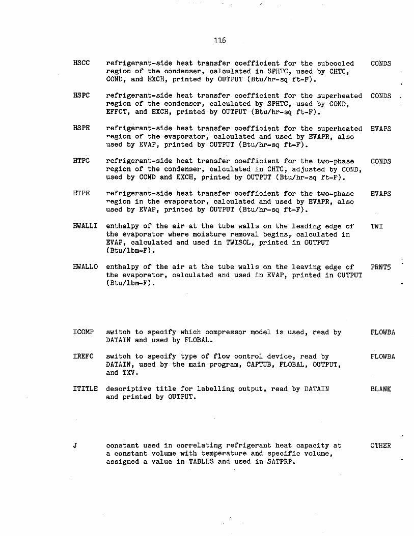
116
HSCC refrigerant-side heat transfer coefficient for the subcooled CONDS region of the condenser, calculated in SPHTC, used by CHTC, . COND, and EXCH, printed by OUTPUT (Btu/hr-sq ft-F). .
HSPC refrigerant-side heat transfer coefficient for the superheated CONDS . region of the condenser, calculated by SPHTC, used by COND, EFFCT, and EXCH, printed by OUTPUT (Btu/hr-sq ft-F).
HSPE refrigerant-side heat transfer coefficient for the superheated EVAPS region of the evaporator, calculated and used by EVAPR, also used by EVAP, printed by OUTPUT (Btu/hr-sq ft-F).
HTPC refrigerant-side heat transfer coefficient for the two-phase CONDS region of the condenser, calculated in CHTC, adjusted by COND, used by COND and EXCH, printed by OUTPUT (Btu/hr-sq ft-F).
HTPE refrigerant-side heat transfer coefficient for the two-phase EVAPS region in the evaporator, calculated and used by EVAPR, also used by EVAP, printed by OUTPUT (Btu/hr-sq ft-F).
HWALLI enthalpy of the air at the tube walls on the leading edge of TWI the evaporator where moisture removal begins, calculated in EVAP, calculated and used in TWISOL, printed in OUTPUT (Btu/lbm-F).
HWALLO enthalpy of the air at the tube walls on the leaving edge of PRNT5 * the evaporator, calculated and used in EVAP, printed in OUTPUT (Btu/lbm-F). .
ICOMP switch to specify which compressor model is used, read by FLOWBA DATAIN and used by FLOBAL.
IREFC switch to specify type of flow control device, read by FLOWBA DATAIN, used by the main program, CAPTUB, FLOBAL, OUTPUT, and TXV.
ITITLE descriptive title for labelling output, read by DATAIN and printed by OUTPUT.
BLANK
constant used in correlating refrigerant heat capacity at OTHER a constant volume with temperature and specific volume, assigned a value in TABLES and used in SATPRP.

117
constant used in refrigeration equations of state correlating STATEQ pressure with temperature and specific volume, assigned a value in TABLES, used by SATPRP, SPVOL, and VAPOR.
.
. .
LElO multiplication constant used to convert logarithms base ten SUPER to natural logarithms, assigned a value in TABLES, used by SATPRP and TSAT.
LPRINT switch to control levels of printed output, read by DATAIN, MPASS used by the main program, COMP, COND, EVAP, EVAPR, and FLOBAL.
LlOE multiplicative constant used to convert natural logarithms SUPER to logarithms base ten, assigned a value in TABLES, used in SATPRP.
. *
MCMPOP switch to specify option for adding heat from the compressor MPASS shell to the air-stream, read by DATAIN, used by COND, EVAPR, and OUTPUT.
MFANFT switch to specify whether or not to use efficiency curve for MPASS the outdoor fan, read by DATAIN, used by the main program, COND, EVAPR, and OUTPUT.
MFANIN switch to specify option for adding heat loss from the indoor MPASS fan to the air-stream, read by DATAIN, used by COND, EVAPR, and OUTPUT.
MFANOU switch to specify option for adding heat loss from the outdoor MPASS fan to the air-stream, read by DATAIN, used by COND, EVAPR, and OUTPUT.
MTRCLC switch used to specify whether or not to calculate the comp- COMPR ressor motor speed, read by DATAIN, used by COMP.
MUNITC switch to specify whether the condenser is the indoor or the CONDEN outdoor heat exchanger, assigned a value by DATAIN -nd used by COND.
. MUNITE switch to specify whether the evaporator is the indoor or the EVAPOR outdoor heat exchanger, assigned a value by DATAIN and used by EVAPR.
c

118
NCAP
NCORH
NR
NSECTC
NSECTE
NTC
NTE
NZTBOP
ORIFD
PA
PC
PCTFL
PDAIRC
number of capillary tubes used, default value assigned in BLOCK DATA, optionally read by DATAIN if capillary tube submodel is used, used by CAPTUB and printed by OUTPUT.
switch to specify heating or cooling mode of operation, read by DATAIN, used by the main program, COND, EVAPR, and OUTPUT.
refrigerant number, assigned a value in BLOCK DATA, used by the main program, MUKCP, SATPRP, TSAT, TXV, and VAPOR.
the number of equivalent parallel refrigerant circuits in the condenser, read by DATAIN, used by OUTPUT, CALC, and COND.
the number of equivalent parallel refrigerant circuits in the evaporator, read by DATAIN, used by EVAPR and OUTPUT.
the number of tubes in the direction of' the air flow in the condenser, read by DATAIN, used by CALC and COND.
the number of tubes in the direction of the air flow in the evaporator, read by DATAIN, used by CALC and EVAPR.
switch to bypass the nozzle and distributor tube pressure drop calculations for the thermostatic expansion valve, assigned a value in BLOCK DATA or read by DATAIN, used by TXV.
diameter of the orifice or short tube, read by DATAIN or calculated by ORIFIC, used by ORIFIC and printed by OUTPUT (ft) l
the atmospheric pressure, assigned a value in BLOCK DATA, used by COND, EVAP, EVAPR, and XMOIST (psia).
inside perimeter of each tube in the condenser, calculated and used in CALC, used in COND (ft).
fraction of the full-lOad,compressor motor power, calculated and used in COMP, printed in OUTPUT.
air-side pressure drop for the condenser, calculated by PDAIR and used by COND and FANFIT, printed by OUTPUT (psi).
FLOWBA
MPASS -
REFRIG
CONDEN
EVAPOR
CONDEN
EVAPOR
TXVDAT
FLOWBA
AIR
CONDEN
PRNTl h
CONDS d

119
PDAIRE air-side pressure drop for the evaporator, initialized to 0 EVAPS in the main program, calculated by PDAIR, used by EVAPR, and printed by OUTPUT (psi).
-5 PDC refrigerant-side pressure drop for the condenser, calculated CONDS
by PDROP in calls from FLOBAL. and COND, used by FLOBAL and COND, printed by OUTPUT (psi).
PDE refrigerant-side pressure drop for each circuit in the evap- EVAPS orator, calculated and.used by EVAPR, printed by OUTPUT (psi).
PE inside perimeter of each tube in the evaporator, calculated EVAPOR and used by CALC, used by EVAPR (ft).
PFLODV pressure of the refrigerant entering the flow control device, PRNT2 calculated and used in FLOBAL, printed in OUTPUT (psia).
PIG pressure of the refrigerant entering the condenser, calculated CONDSR in COMP, modified by DESUPR and FLOBAL, used by COMP and COND, printed by OUTPUT (psia).
PIE pressure of the refrigerant entering the evaporator, calc- EVAPTR ulated and used by EVAPR, also calculated and used by TXV, printed by OUTPUT (psia).
PINCMP pressure of the refrigerant at the compressor shell inlet calculated and used in COMP or CMPMAP, printed in OUTPUT (psia).
CMPRSR
POC pressure of the refrigerant leaving the condenser, calculated CONDSR in COND and FLOBAL, used by COND and FLOBAL, printed by OUTPUT (psia).
POE pressure of the refrigerant leaving the evaporator, calculated EVAPTR and used by COMP, used by EVAPR and TXV, printed by OUTPUT (psia).
POUCMP pressure of the refrigerant at the compressor shell outlet calculated and used in COMP or CMPMAP, printed in OUTPUT (psia).
CMPRSR
POW compressor power consumption, computed and used in COMP, used COMPR in the main program, printed by OUTPUT (kW).
POW2 rate of power consumption by the compressor, calculated and PRNT8 used by the main program, printed by OUTPUT (Btu/hr).
. PRA Prandtl number of air, calculated and used by COND and EVAPR. AIR
l PRINT logical variable to control the output of intermediate Al
calculations, set to TRUE or FALSE in the main program depending on the value of LPRINT.
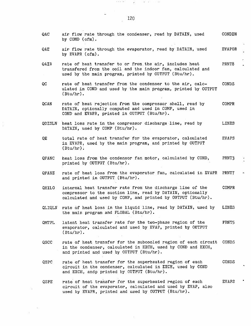
- 120
QAC air flow rate through the condenser, read by DATAIN, used CONDEN by COND (cfm).
QAE air flow rate through the evaporator, read by DATAIN, used EVAPOR by EVAPR (cfm).
A
QAIR rate of heat transfer to or from,the air, includes heat PRNT8 _ transfered from the coil and the indoor fan, calculated and used by the main program, printed by OUTPUT (Btu/hr).
QC rate of heat transfer from the condenser to the air, calc- CONDS ulated in COND and used by the main program, printed by OUTPUT (Btu/hr).
QCAN rate of heat rejection from the compressor shell, read by COMPR DATAIN, optionally computed and used in COMP, used in COND and EVAPR, printed in OUTPUT (Btu/hr).
QDISLN heat loss rate in the compressor discharge -line, read by DATAIN, used by COMP (Btu/hr).
LINES
QE total rate of heat transfer for the evaporator, calculated in EVAPR, used by the main program, and printed by OUTPUT (Btu/hr).
EVAPS
QFANC heat loss from the condenser fan motor, calculated by COND, PRNT3 - printed by OUTPUT (Btu/hr).
I
QFANE rate of heat loss from the evaporator fan, calculated in EVAPR PRNT7 I and printed in OUTPUT (Btu/hr).
QHILO internal heat tra,nsfer rate from the discharge line of the COMPR compressor to the suction line, read by DATAIN, optionally calculated and used by COMP, and printed by OUTPUT (Btu/hr).
QLIQLN rate of heat loss in the liquid line, read by DATAIN, used by LINES the main program and FLOBAL (Btu/hr).
QMTPL latent heat transfer rate for the two-phase region of the PRNTfj evaporator, calculated and used by EVAP, printed by OUTPUT (Btu/hr).
QSCC rate of heat transfer for the subcooled region of each circuit CONDS in the condenser, calculated in EXCH, used by COND and EXCH, and printed and used by OUTPUT (Btu/hr).
QSPC rate of heat transfer for the superheated region of each CONDS circuit in the condenser, calculated in EXCH, used by COND .
and EXCH, andp printed by OUTPUT (Btu/hr).
QSPE rate of heat transfer for the superheated region of each EVAPS ' circuit of the evaporator, calculated and used by EVAP, also used by EVAPR, printed and used by OUTPUT (Btu/hr).

121
QSTPT
. QSUCLN
4
QTPC
QTPE
R
RACKS
RAU
RESIST
RHI
RHIC
RHIE
RHO
RHTERM
RPM
sensible heat transfer evaporator, calculated (Btu/hr).
rate for the two-phase region of the and used in EVAP, printed by OUTPUT ._... ...____-..".._. _ . I
PRNT5
rate of heat gain in the suctin line between the evaporator LINES ‘ . ". .,.. , ., . and the compressor, read by DATAIN and used by either'CMPMAP- or COMP (Btu/hr).
rate of heat transfer for the two-phase region of each CONDS circuit in the condenser;“"'
-. ‘.,. (.*xIW -I .._ _ "~1 .^ "_- calculated and used in-‘%XCH*, used
by COND, printed by OUTPUT (Btu/hr).
rate of heat transfer for the two-phase region of each circuit EVAPS of the evaporator, calculated and used by EVAP, also assigned a value and used by EVAPR, printed by OUTPUT (Btu/hr).
constant used in refrigerant equations of state correlating STATEQ pressure with temperature and specific volume, assigned a value in TABLES, used by SATPRP, SPVOL, and VAPOR.
number of racks of resistance heaters, assigned a value in BLOCK DATA and used in PDAIR.
AIR
universal gas constant for air, assigned a value in BLOCK DATA, used by COND and EVAPR (ft-lbf/lbm-R).
AIR
amount of resistance heat-required to meet the house load, calculated and used in the main program, printed by.OUTPUT (Btu/hr).
PRNT8
the relative humidity of the air entering the evaporator coil, PRNT5 calculated and used in EVAP, printed in OUTPUT.
the relative humidity of the air entering the condenser unit, CONDEN read by DATAIN and used in COND and EXCH.
the relative humidity of the air entering the evaporator unit, EVAPOR read by DATAIN, used by EVAP and EVAPR.
relative humidity of the air at the leaving edge of the PRNT5 evaporator, calculated and used by EVAP, printed by OUTPUT.
constant in dehumidificati-on solution, calculated in EVAP and used in TWOSOL.
TWO
actual compressor motor speed, assigned a value and used in ,PRNTl COMP, printed by OUTPUT (rpm's).

122
RPMFAN motor speed for the outdoor fan, assigned a value in BLOCK FANMOT DATA, used by FANFIT (rpm's).
. RPMSLP slope of the linear fit to the fraction of no-load compressor CMPMOT
motor speed as a function of fraction of full-load power, assigned a value in BLOCK DATA and used in COMP.
RTBCND the number of return bends in the condenser, read by DATAIN, CONDEN scaled and used by CALC.
RTBEVP the number of return bends in the evaporator, read by DATAIN, EVAPOR scaled and used by CALC.
RTOT overall resistance to heat transfer for the superheated region EFFARG of the condenser (l/UA), calculated in EFFCT and used by EXCH (hr-F/Btu).
SEFFD overall surface efficiency for hexagonal fins (staggered tubes) EVAPRS in the evaporator, calculated and used in EVAP, used by EVAPR, and printed by OUTPUT.
SEFFWA average surface efficiency for the portion of the evaporator EVAPRS where moisture removal occurs, calculated and used in EVAP, used in EVAPR, and printed in OUTPUT.
SEFFXC overall surface efficiency for the condenser, calculated in CONDS SEFF, and used by COND, EFFCT, and EXCH.
SIGAC ratio of the free flow frontal area of the condenser to the CONDEN total frontal area, calculated in CALC and used in COND.
SIGAE ratio of the free flow frontal area of the evaporator to the EVAPOR total frontal area, calculated in CALC and used in EVAPR.
ss specific speed of the outdoor fan , calculated in FANFIT and PRNT8 printed by OUTPUT.
STATIC static superheat setting for, the thermostatic expansion TXVDAT valve, assigned a value in BLOCK DATA or read by DATAIN, used by TXV and printed by OUTPUT (F).
STC vertical spacing between tube passes in the condenser, read CONDEN by DATAIN, used by CALC and COND (ft).
STE vertical spacing between tube passes in the evaporator, read EVAPOR by DATAIN, used by CALC, EVAP, and EVAPR (ft).
STRTOT ratio of the sensible to total heat transfer rates for the evaporator, calculated in EVAP, printed by OUTPUT.
PRNT5

123
STRTP
.
SUCFAC e
SUPER
SUPERB
.
SUPRAT
SYNC
TACI
TAIC
TAIE
TAIIC
TAIIE
TAOC .
TAOE L
ratio of the sensible to .total heat !?zS?z.,rate?. .,., for.. the. ._ two-phase region of the evaporator, calculated in EVAP and printed in OUTPUT.
correction factor for suction gas heating in the compressor, assigned a value in BLOCK DATA and used in CMPMAP.
specified superheat of the refrigerant leaving the evaporator read by DATAIN, used by COMP, EVPTR, OUTPUT, and TXV (F).
base superheat value for the compressor map, read by DATAIN and used by CMPMAP (F).
rated operating superheat for the thermostatic expansion valve, assigned a value in BLOCK DATA or read by DATAIN, used by TXV, and printed by OUTPUT (F).
synchronous or actual compressor motor speed depending on whether or not the full load motor power is calculated, read in DATAIN and used in COMP (rpm's).
temperature of the air at the point where moisture removal begins, calculated and used in EVAP, printed in OUTPUT (F).
temperature of the air crossing the condenser, includes any
PRNT5
MAPFIT
FLOWBA
MAPFIT
TXVDAT
COMPR
PRNT5
PRNT3 heat losses from the fan motor or compressor, calculated in COND and printed in OUTPUT (F).
air temperature crossing the evaporator coil, inlet air PRNT7 temperature with any additions due to fan motor and compressor heat losses, calcul.ated in EVAPR and printed in OUTPUT (F).
air temperature entering the condenser, read by DATAIN, used CONDSR by COND and EFFCT, printed by OUTPUT (F).
air temperature entering the evaporator which corresponds to EVAPTR the current values of TSATEI and TSATEO, the desired value for the ambient air temperature is read by DATAIN, current value is calculated and used by the main program, also used by EVAPR, EVPTR, and OUTPUT, printed by OUTPUT (F).
air temperature after it passes over the condenser coil, calc- CONDSR ulated in EXCH, used by COND, and printed in OUTPUT (F).
air temperature leaving the evaporator with any additions for EVAPTR compressor and fan motor heat losses, calculated and used by EVAP, used by EVAPR, and printed by OUTPUT (F).

124
TAOOC air temperature leaving the condenser, includes any heat losses PRNT3 from the compressor and fan motors, calculated in COND and printed in OUTPUT (F).
TAOOE air temperature leaving the evaporator, includes any additions PRNT7 due to heat losses from the fan and compressor motors, calc- ulated in EVAPR and printed in OUTPUT (F).
TAOSC outlet air temperature from the subcooled region of the PRNT4 condenser, calculated in EXCH, printed in OUTPUT (F).
TAOSPC outlet air temperature from the superheated region of the condenser, calculated in EXCH, printed in OUTPUT (F).
PRNT4
TAOSPE outlet air temperature from the superheated region of the PRNT5 evaporator, calculated and used in EVAP, printed in OUTPUT (F).
TAOTPC outlet air temperature from the two-phase region of the cond- PRNT4 endser, calculated in EXCH, printed in OUTPUT (F).
TAOTPE outlet air temperature from the two-phase region of the evap- PRNT5 orator, calculated and used in EVAP, printed in OUTPUT (F).
TC critical temperature for the refrigerant, assigned a value in SUPER TABLES, used in SATPRP, SPVOL, and VAPOR (R).
TERAT evaporating temperature used for rating the thermostatic TXVDAT expansion valve, assigned a value in BLOCK DATA, used in TXV (F).
TFLODV refrigerant temperature entering the flow control device, talc- PRNT2 ulated and used in FLOBAL, printed in OUTPUT (F).
TFR constant used to convert from Farenheit to absolute tempera- SUPER ture when using correlations for refrigerant properties (i.e. the value assumed by researcher deriving the correlation), assigned a value in TABLES, used by SATPRP, SPVOL, TSAT, and VAPOR (F).
TIC temperature of the refrigerant entering the condenser, initial- CONDSR ized by COMP, calculated in DESUPR and COMP, used by COND, DESUPR, EFFCT, and EXCH, printed by OUTPUT (F).
TIE temperature of the refrigerant entering the evaporator, EVAPTR calculated by EVAPR and printed by OUTPUT (F).
TLQCOR correction factor to adjust tube and nozzle pressure drops TXVDAT in the thermostatic expansion valve for liquid temperatures entering the valve other than the rating temperature, calc- ulated and used in TXV, printed in OUTPUT.

125
TLQRAT
I TOLH
TOLS
TRICMP
TROC
TROCMP
TROE
TRVDS
TSATCI
TSATCO
TSATEI
TSATEO
.
t TSATFL
rating temperature of the.liquid refrigerant at the inlet to the thermostatic expansion valve, assigned a value in BLOCK DATA and used in TXV (F).
tolerance parameter used to calculate superheated vapor properties when the two known properties are the pressure and enthalpy, assigned a value in BLOCK DATA used by COMP. _... .~ _--..-..._ .,.,f
tolerance parameter used to calculate superheated vapor . .)_, properties when the two known properties are pressure and entropy, assigned a value in BLOCK DATA and used by COMP.
temperature of the refrigerant at the compressor shell inlet calculated and used in COMP or CMPMAP, printed in OUTPUT (F).
temperature of the refrigerant at the condenser exit, esti- mated in FLOBAL, calculated in EXCH, used by CNDNSR, COND, FLOBAL, and FLODEV, printed in OUTPUT (F).
temperature of the refrigerant at the compressor shell outlet calculated in COMP or CMPMAP, printed in OUTPUT (F).
temperature of the refrigerant leaving the evaporator, calc- ulated and used in EVAP, used by EVAPR and EVPTR, printed by OUTPUT (F).
TXVDAT
MPASS
MPASS
CMPRSR
CONDSR
CMPRSR
EVAPTR
refrigerant temperature at the end of the desuperheating region CONDS in the condenser, initialized in COND, calculated by EXCH, and used by COND, EFFCT, and EXCH (F).
saturation temperature of the refrigerant entering the conden- CONDSR ser, initial guess read by DATAIN, calculated in the main program, used by COMP, FLOBAL, COND, EXCH, and DESUPR, printed by OUTPUT (F).
saturation temperature of the refrigerant leaving the conden- CONDSR ser calculated in COND and FLOBAL, used by CNDNSR, COND, EXCH, FLOBAL, and FLODEV, printed in OUTPUT (F).
saturation temperature of the refrigerant entering the evap- EVAPTR orator, initialized in the main program, calculated and used by EVAPR and TXV, printed by OUTPUT (F).
saturation temperature of the refrigerant leaving the evap- EVAPTR orator, initial guess read by DATAIN, calculated and used by the main program, used by COMP, EVAPR, EVPTR, FLOBAL, and TXV, printed by OUTPUT (F).
saturation temperature of the refrigerant entering the flow PRNT2 control device, calculated and used in FLOBAL, printed in OUTPUT (F).

126
TSATRl
TSATR2
TSICMP
TSOCMP
TWALLI
TWALLO
TWBI
TWBO
TXVRAT
UATPAW
UATPW
ULA
V
average saturation temperature in the evaporator, assigned a value in EVAP, used in TWISOL (F).
average saturation temperature in the evaporator, assigned a value in EVAP, used by TWOSOL (F).
saturation temperature of the refrigerant at the compressor shell inlet calculated and used in COMP or CMPMAP, printed in OUTPUT (F).
saturatin temperature of the refrigerant at the compressor shell outlet calculated in COMP or CMPMAP, printed in OUTPUT (F).
tube wall temperature at the leading edge of the evaporator where moisture removal begins, calculated and used in EVAP, used by TWOSOL, printed in OUTPUT (F).
air temperature at the tube walls on the leaving edge of the evaporator, calculated and used in EVAP, printed in OUTPUT (F).
TWI
Two *
7
CMPRSR
CMPRSR
TWO
PRNT5
wet bulb temperature of the air entering the evaporator, calc- PRNT5 ulated in EVAP, printed in OUTPUT (F).
wet bulb temperature of the air at the leaving edge of the evaporator, calculated in EVAP, printed in OUTPUT (F).
PRNT5
rated capacity of the thermostatic expansion valve, assigned TXVDAT a value in BLOCK DATA and used in TXV (tons).
air-side thermal conductance times the heat transfer area (UA) UAS for the portion of the two-phase region of the evaporator which is wetted due to dehumidification, calculated in EVAPR, and printed in OUTPUT (Btu/hr-F).
refrigerant-side thermal conductance times the heat transfer UAS area (UA) for that portion of the two-phase region of the evaporator whose outside surface is wetted due to dehumidifi- cation, calculated in EVAPR and printed in OUTPUT (Btu/hr-F).
upper limit on the Reynold's number for laminar flow of the VAPHTC refrigerant, assigned a value in BLOCK DATA and used in SPHTC.
constant in dehumidification solution, calculated in EVAP and used in TAOSOL and TWOSOL.
TWO
127
VOLFAC I
- VR
W
WAIRI
WAIRO
WOUT
WTC
. L WTE
. . WWALLI
WWALLO
X
XFLODV
XIC
XIE
correction factor for the compressor volumetric efficiency, assigned value in BLOCK DATA and used in CMPMAP.
compressor clearance volume ratio, read by DATAIN and COMPR used by COMP.
constant in dehumidification solution, calculated in EVAP and used in TAOSOL and TWOSOL.
humidity ratio of the air at the leading edge of the evapor- ator calculated and used in EVAP, printed in OUTPUT.
humidity ratio of the air leaving the evaporator, calculated and used in EVAP, printed in OUTPUT.
humidity ratio of the 'air at the leaving edge of the evap- orator, calculated and used by EVAP, printed by OUTPUT.
spacing of the tubes in the condenser in the direction of air flow, read by DATAIN, used by CALC and COND (ft).
spacing of the tubes in the evaporator in the direction of the air flow, read by DATAIN, used by EVAP and EVAPR (ft).
humidity ratio at the tube walls on the leading edge of the evaporator where moisture removal begins, calculated and used in EVAP, calculated in TWISOL, printed in OUTPUT.
humidity ratio of the air at the tube walls on the leaving edge of the evaporator, in OUTPUT.
calculated and used in EVAP, printed
constant used in correlating enthalpy of refrigerant vapor with temperature and specific volume, assigned a value in TABLES and used in SATPRP.
vapor quality of the refrigerant entering the flow control device, calculated in FLOBAL and printed in OUTPUT.
refrigerant vapor quality entering the condenser, set to 1.0 in FLOBAL, modified in DESUPR, used by COND and EXCH, printed in OUTPUT.
refrigerant vapor quality entering the evaporator, calculated and used in EVAPR and printed in OUTPUT.
MAPFIT
TWO
PRNT5
PRNTS
PRNT5
CONDEN
EVAPOR
TWI
PRNT!j
OTHER
PRNT2
CONDSR
EVAPTR

128
XINCMP
XKFC
XKFE
XLCORR
XLLR
XLEQDL
XLEQHP
XLEQLL
XLEQLP
XLEQSL
XMAC
XMAE
XMASP
XMATP
XMM
refrigerant vapor quality at the compressor shell inlet calculated and used in COMP or CMPMAP, printed in OUTPUT.
thermal conductivity of the fins in the condenser, read by DATAIN, used by CALC and COND (Btu/hrFt-F).
thermal conductivity of the fins in the evaporator, read by DATAIN, used by CALC and EVAP (Btu/hr-ft-F).
correction factor for the pressure drop in distributor tubes of the thermostatic expansion valve for tubes of lengths other than the rated length, calculated and used in TXV, printed in OUTPUT.
lower limit on the Reynold's number for laminar flow of the refrigerant, assigned a value in BLOCK DATAand used in SPHTC.
equivalent length of the compressor discharge line from the reversing valve to the condenser, read by DATAIN -nd used by COMP (ft).
CMPRSR -
CONDEN r
EVAPOR
TXVDAT
VAPHTC
LINES
equivalent length of the high pressure line from the compressor LINES discharge port to the reversing valve, read by DATAIN and used by COMP (ft).
equivalent length of the liquid line connecting the indoor and LINES outdoor heat exchangers, read by DATAIN -nd used by FLOBAL (ft).
equivalent length of the low pressure line from the compressor LINES suction port to the reversing valve, read by DATAIN and used by COMP (ft).
equivalent length of the suction line from the evaporator to LINES the reversing valve, read by DATAIN -nd used by COMP (ft).
mass flow rate of air across each parallel circuit in the CONDS condenser, calculated in COND, used by EFFCT and EXCH, printed in OUTPUT (lbm/hr).
mass flow rate of airy across each parallel circuit in the evaporator, calculated in EVAPR and used in EVAP, printed in OUTPUT (lbm/hr).
EVAPS
mass flow rate of the air across the superheated region of PRNT5 each circuit in the evaporator, calculated and used in EVAP, printed in OUTPUT (lbm/hr).
mass flow rate of the air across the two-phase region of PRNT5 each circuit in the evaporator, calculated and used in EVAP, printed in OUTPUT (lbm/hr).
rate of moisture removal from the air, calculated in EVAP and PRNT5 printed in OUTPUT (lbm/hr).

129
XMR refrigerant mass flow rate, initial guess or estimate read by FLOBAL DATAIN, calculated in COMP, used by the main program, COND, EFFCT, EVAPR, FLOBAL, and the flow control device subroutines, printed and used by OUTPUT (lbm/hr).
XMUA viscosity of air, calculated and used by COND and EVAPR AIR (lbm/hr-ft).
XNTUSC number of transfer units for the subcooled region of the condenser, calculated in EXCH, printed in OUTPUT.
PRNT4
XNTUSP number of heat transfer units for the superheated region of PRNT4 the condenser, calculated and used in EXCH, printed in OUTPUT.
XNTUSU number of heat transfer units for the superheated region of PRNT5 the evaporator, calculated and used in EVAP, printed in OUTPUT.
XNTUTP number of heat transfer units for the two-phase region of PRNT4 the condenser, calculated and used in EXCH, printed in OUTPUT.
XNTUTP number of heat transfer units for the two-phase region of PRNT5 the evaporator, calculated and used in EVAP, printed in OUTPUT.
. c xoc refrigerant vapor quality leaving the condenser, initialized CONDSR
in COND, calculated in EXCH, used by CNDNSR, COND, EXCH, FLOBAL, and FLODEV, printed in OUTPUT.
c XOE vapor quality of the refrigerant leaving the evaporator, EVAPTR calculated and used in EVAPR, used in EVPTR and COMP, and printed in OUTPUT.
XOUCMP refrigerant vapor quality at the compressor shell outlet calculated in COMP or CMPMAP and printed in OUTPUT;
CMPRSR
Y constant used in correlating entropy of refrigerant vapor with temperature and specific volume, assigned a value in TABLES and used in SATPRP.
OTHER

/ ,

131
Appendix E - Cross-Reference of Common Blocks
The common
data to or from
marks.
blocks listed in the rows of Table 1 are used to transmit
the subroutines identified by the columns with the "X1'

132
SUBROUTINES
AIR
Al
BLANK
CMPMOT
CMPRSR
COMPR
CONDEN
CONDS
CONDSR
DENSIT
EFFARG
EVAPOR
EVAPRS
EVAPS
EVAPTR
FANMOT
FLOWBA
LINES
MAPFIT
MPASS
OTHER
PRNTl
PRNTZ
PRNT3
PRNT4
PRNT5
PRNT7
PRNT8
REFRIG
SAT
STATE4
SUPER
TWI
TWO
TXVDAT
UAS
VAPHTC
I iii/iii/
I 1x1 I lxlxl I
I I I I I I lxlxl 1
I I IXIXI I lxlxl I I I 1x1 I I I 4 I I I I I I I 4 I I I I
I lxlxl Ixlxlxl I I 1x1 Ixlxlxl I I 1x1 1 X I I r. x X
I XII IIII 1,x,,, ,,,,, ,,,. X

133
Appendix F - Subroutine Descriptions and Cross-Reference of Subroutine Calls
Subroutine Descriptions
Main Program serves as driving program for high- and low-side computa- tions and contains iterative loop converging on evaporator inlet air temperature
BLOCK DATA assigns values to constants and infrequently changed
CALC
CAPTUB
CHTC
CMPMAP
CNDNSR
COMP
COND
DPF
DPFSOL
DPLINE
EFFCT
h
5 EHTC
parameters
calculates geometric constants for both heat exchangers
submodel for capillary tube flow rate
calculates refrigerant-side heat transfer coefficient for the two-phase region of the condenser
computes refrigerant mass flow and compressor power consumption from compressor map data
serves as ,driving routine for COMP, COND and FLOBAL and returns the difference between the calculated and specified condenser subcooling or between the compressor and expansion device re- frigerant mass flow rates
computes refrigerant mass flow rate and compressor power con- sumption from efficiency and loss parameters
calculates total condenser heat transfer rate, air and refriger- ant properties and refrigerant and air-side pressure drops for fixed inlet refrigerant conditions
determines an approximate dew-point temperature for a given vapor pressure of moist air
calculates the difference between the known saturation pressure of water vapor at the tube wall and the saturation pressure corresponding to an estimated, or given tube wall temperature
determines the single-phase pressure drop in the refrigerant lines
computes the difference in condenser effectiveness values between the general effectiveness equation and the specific cross-flow effectiveness equation as a function of the fraction of the coil, fV, containing superheated refrigerant vapor
calculates refrigerant-side heat transfer coefficient for the two-phase region of the evaporator

134
EVAP
EVAPR
EVPTR
EXCH
EXF
FANFIT
FLOBAL
FRICT
GUESS2
GUESS3
INTER
HAIR
MUKCP
MUKCPA
OR1 FIC
OUTPUT
determines the heat transfer, moisture removal, and outlet air temperatures and humidities from one circuit of the evaporator for given heat transfer coefficients and saturation temperatures at the beginning and end of the two-phase region
calculates evaporator heat transfer rate, air and refrigerant properties, and refrigerant and air-side pressure drops for fixed exit refrigerant conditions
serves as a driving routine for EVAPR and returns the difference between the specified evaporator superheat and the calculated value
determines the heat transfer and outlet temperatures for one circuit of the condenser for given heat transfer coefficients and saturation temperatures at the beginning and end of the two-phase region
determines the effectiveness of a cross-flow heat exchanger using the effectiveness - NTU method
calculates combined fan-fan motor efficiency given air-side pressure drop and volumetric air-flow rate
determines refrigerant conditions at the inlet to the flow control device and drives the expansion device models
computes the general Moody friction factor for s flow in tubes
ingle phase
brackets a solution prior to using a root finder end points by factors of 10
by shifting
brackets a solution prior to using a root finder end points by constant step
by shifting
interpolate in a single dimension using Lagrangian polynomial
computes air-side heat transfer coefficient for smooth fin and tube geometry
calculates viscosity, thermal conductivity, and specific heat of 13 refrigerants
calculates viscosity, thermal conductivity, and specific heat of air
computes refrigerant mass flow rate through a short-tube orifice
prints a detailed summary of output data

135
a
PDAIR
PDRQP
PVSF
SATPRP
SEFF
SLAG
SPFHT
SPHTC
SPHTCZ
SPVOL
SUPCOR
TABLES
TAOSOL
TRIAL
TSAT
TWISOL
TWOSOL
TXV
calculates air-side pressure drop for smooth, wavy, or louvered fin and tube heat exchangers
determines single- and two-phase pressure drops for flow in heat exchanger tubes
calculates partial pressure of water vapor in saturated air
evaluates the saturation thermodynamic properties of a specified refrigerant
determines surface efficiency for a hexagonal shaped fin surface
computes single precision Lagrangian interpolation in two dimensions from tabulated data
calculates refrigerant specific heats at constant pressure and volume and specific heat ratio
computes single-phase heat transfer coefficient for laminar, transition, or turbulent gas flow from an abrupt contraction entrance
computes single-phase heat transfer coefficient for fully developed liquid or gas flow
evaluates specific volume of superheated refrigerant
calculates power and mass flow correction factors for map- based compressor model to correct for superheat level
assigns constants for refrigerant thermodynamic property sub- routines
computes the exit air temperature from the region of the evaporator where moisture removal occurs
determines thermodynamic properties of superheated refrigerant vapor given two known properties
'calculates saturation temperature of refrigerant given satura- tion pressure
used to compute the wall temperature at which moisture removal begins on the leading edge of the evaporator
used to compute the wall temperature at the exit from the evaporator
computes the refrigerant mass flow rate through a thermostatic expansion valve
1 3-6
VAPOR determines thermodynamic properties of superheated refrigerant vapor given temperature and pressure
WBF determines wet-bulb temperature of moist air
WTSFIT computes coefficients for a quadratic fit of wall temperature to enthalpy of moist air
XMOIST calculates dew point temperature, humidity ratio enthalpy, and wet-bulb temperature or relative humidity of moist air
ZERO's each of these routines solves for the root, or zero, of a function from two points which bracket the solution using bi- section and Newton's method
The subroutines listed in the columns of Table F.1 are called from
the subprograms listed in the rows of Table F.1 which are indicated by
"X'S".

137
. .
+,


139
Appendix G - Algebraic Notation
A
a
A a
A contact
Af
A filter
A ft
A heater
A min
A orifice
A r
A rh
A side
A tubes
A 0
b
b fat
C
C a
C fat
C max
C min
frontal area of heat exchanger
intercept of a linear fit to data which is determined by context
air-side fin and tube heat transfer area
total contact area between fins and tubes
air-side fin heat transfer area
frontal area of filter on indoor unit
air-side fin and tube heat transfer area
cross-sectional area of the resistance heater section
ratio of total air-side heat transfer area to the minimum free-flow area
cross-sectional area of the short tube orifice
total refrigerant-side heat transfer area
refrigerant-side heat transfer area for each parellel circuit
heat transfer area of each side of each fin
total exposed surface area of tubes in heat exchanger
refrigerant-side heat transfer area per unit air flow rate
slope of a linear fit to data which is determined by context
bypass or bleed factor for a thermostatic expansion valve
compressor piston clearance volume ratio or expansion device flow area coefficient or Dittus-Boetter exponent
heat capacity rate of air (macPa)
ratio of humidity ratio gradient to the temperature gradient
maximum of the heat capacity rates for the air and the refrigerant
minimum of the heat capacity rates for the air and the refrigerant

140
C r
C
C P
C pa
C pm
C r
C 0
D
d
D a
D ducts,
D r
f
F a
F moist
F P
F sh
f tot
F W
f wet
F
Fktt)
heat capacity rate of refrigerant (mrcp)
constant in Eq. 6.15
specific heat of the refrigerant
specific heat of air
specific heat of moist air
heat capacity rate of the refrigerant
correction factor to the air-side heat transfer coefficient for wavy and louvered fins
total compressor piston displacement or refrigerant tube diameter depending on context
depth of heat exchanger
air-side or outer diameter of heat exchanger tubes
diameter of air ducts
refrigerant-side or inner diameter of heat exchanger tubes
fraction of rated value, fraction of coil, or friction factor determined by context
fin heat transfer area per unit total air-side heat transfer area
fraction of that part of the evaporator which is in two-phase flow that is wetted due to dehumidification
fin pitch
compressor suction gas heating factor
combined wet and dry friction factor for the evaporator
fraction of the evaporator that is wetted due to dehumidification
friction factor for the region of the evaporator which is wetted due to dehumidification
compressor volumetric efficiency correction factor
correlating function for the refrigerant-side two-phase heat transfer coefficient
r F*
. G
. *
SC
h
h a,s
h a, a,
h fg
h' f g
h
h ave
‘d
h tP
h W
h* W
%
h2
k
L
e
L exposed
c tubes
ril
l I m
141
correlating parameter
mass flux
gravitational acceleration constant
enthalpy of refrigerant or height of heat exchanger
enthalpy of saturated air at wall surface temperature
enthalpy of moist air at freestream conditions
latent heat of vaporization
driving enthalpy difference in the condenser
air or refrigerant heat transfer coefficient (determined by subscript or context)
average condensation heat transfer coefficient
mass transfer coefficient
average condensing or evaporating heat transfer coefficient (condensation value includes an adjustment due to Rohsenow)
sensible heat transfer coefficient for a wetted surface
effective heat transfer coefficient for a wet surface
local evaporation heat transfer coefficient using Chaddock- Noerager correlation
local evaporation heat transfer coefficient for the dry-out region using nonlinear interpolation between the Chaddock- Noerager value at xdo and the value for saturated vapor
thermal conductivity
equivalent length of refrigerant pipes
length of tubes in heat exchangers
length of tubes in heat exchanges exposed to the air
equivalent length of distributor tubes in thermostatic expansion valve
mass flow rate
mass flow rate at "standardized" test or rating conditions

, . .-.
N cap
N circuits
Nf
N Le
N Pr
N Re
NT
f N tot
/ NtU
N V
P
6
6 can
6 cooling
'hilo
R
r
I
rl
S
S heat exchanger coil characteristic
S oper
S S
S sync
142
number of parallel capillary tubes
number of equivalent parallel refrigerant circuits in the heat exchanger
total number of fins in the heat exchanger
Lewis number
Prandtl number
Reynolds number
number of tube rows in the heat exchanger in the direction of the air flow
total number of tubes in the heat exchanger
number of heat transfer units
number of tubes stacked vertically in the heat exchanger
pressure
heat transfer rate
rate of. heat rejection from the compressor shell
rate of heat transfer from the compressor and compressor motor to the suction gas
rate of heat transfer from the compressor discharge line to the suction gas
volumetric air flow rate
thermal resistance per unit of refrigerant side-area
ratio of UA values used in Eq. 6.11
ratio of UA values used in Eq. 6.23
motor speed
actual or operating motor speed
specific speed of the fan for the outdoor heat exchanger
synchoronous speed of compressor motor

143
.
3 T
T aid
T aie
T v,ds
T sat
U
V hx
W
i
w m a, i
fan
I; s,fl
wT
X
X tt
c1 a
cx can
a corr
ahilo
01 r
a racks
vertical spacing between tubes in heat exchanger
air or refrigerant temperature (determined by context)
evaporator inlet air temperature for which dehumidification would occur at the finned tube surface
temperature of the air entering the evaporator
bulk refrigerant vapor temperature at the start of the desuper- heating region of the condenser
refrigerant saturation temperature
thermal conductance
volume of space occupied by heat exchanger
humidity ratio
work performed or energy input
humidity ratio of air at freestream conditions
fan motor power consumption
compressor-motor full load shaft power
spacing of heat exchanger tubes in the direction of air flow
refrigerant vapor quality
correlating parameter for two-phase heat transfer coefficient
total air-side heat transfer area per unit heat exchanger volume
fraction of the compressor power consumption which is rejected from the shell to the ambient air
correction factor for liquid refrigerant temperatures at the inlet to a thermostatic expansion valve other than 100°F
fraction of compressor power consumption transferred from the discharge line to the suction line
total refrigerant-side heat transfer area per unit heat exchanger volume
correction factor to adjust air-side pressure drop for the number of resistant heater racks

B corr
Y
6
Ah
Af’
APJ3 0 2
AT
E
E cf
n
1-I
V
P
0
u a
Subscripts
a
actual
ave
cm
d
do
dp
144
correction factor for TXV distributor tube lengths other than 30 inches
ratio of specific heat at constant pressure to specific heat at constant volume
fin thickness
enthalpy change
pressure drop
pressure drop measured in inches of water
temperature difference, level of subcooling, or level of superheat depending on context
heat exchanger effectiveness
effectiveness of a counter-flow heat exchanger
compressor efficiency or heat exchanger overall surface effectiveness
viscosity
specific volume
density
capillary tube flow factor
free-flow frontal area per unit total frontal area of heat exchanger -
air
at modeled operating conditions
average
compressor
dry
dry-out point in the evaporator where there is no longer a liquid film on the tube wall
dew point

145
eff
evap
f
fl
frict
ft
i
in
inlet
isen
R
lot
m
map
max
mech
mom
noz
0
oper
out
outlet
r
rated
rb
S
effective
evaporator
fin
compressor motor full load
friction
fin and tube
heat exchanger inlet
entering
compressor shell inlet
isentropic
liquid
local
mean
from compressor map
maximum
mechanical
momentum
TXV nozzle
heat exchanger outlet
at modeled operating conditions
exiting
compressor shell outlet
refrigerant
at rating conditions
return bends
compressor shaft

, . - - , , .~ ._ . -^,“l . _ . . - “__l^_._-“...
sat
sh
static
t
tP
tubes
TXV
V
vol
w
co
146
saturation
suction gas heating
static fan efficiency or static superheat value of a thermo- static expansion valve
tube
two-phase
heat exchanger or TXV distributor tubes
thermostatic expansion valve
vapor
volumetric
region wetted due to dehumidification
freestream condition
L

147
Appendix H - Derivation of Dehumidification Solution
H.l Introduction
A method is described in this section for computing the performance
of an air-to-refrigerant evaporator under dehumidification conditions.
The method represents an assimilation and/or expansion of the work of
Goodman [H.l], McElgin and Wiley [H.2], Hiller and Glicksman [H.3],
Threlkeld [H.4], and McQuiston [H.5, H.61, and uses wet heat transfer
coefficients derived from dry heat transfer values via the equation of
Myers [H.7] as noted in Section 6.
H.2 Heat Transfer Equations -Air to Wall
The local driving force for simultaneous heat and mass transfer can
be described, using simplifying assumptions, by Eq. H.l [H.6]
db = h, (h a, to -ha ,JdAs ,
where
dQ - a differential quantity of local heat and mass transfer
‘d - the mass transfer coefficient
h m - a, the enthalpy of humid air at the freestream condition
h a,s -
the enthalpy of saturated air at the wall surface tem- perature
dA - a differential element of wetted surface area. S
Equation H.l contains the assumption that the Colburn analogy, given by
Eq. H.2 CH.61,
h W =
’ ‘d
N 213 Le
pm (H-2)

148
where
h - sensible heat transfer coefficient for a wetted surface W
c - pm
moist air specific heat, c = c pm pa
+ .444 wa,co
woo - a, humidity ratio of air, and
N Le - Lewis number,
holds and that (MLe)2'3 c: 1. Also, the energy content of the condensate
is neglected and the effect of the water film thickness is ignored
(except for the effect on the sensible heat transfer coefficient for a
wetted surface). There are analyses in the literature by Threlkeld
[H.4] and Elmahdy [~.8] which do not require some or all of these
assumptions; however, these analyses were judged too complicated for use
with the simplified heat exchanger routines in the heat pump model.
Equation H.l is strictly applicable for describing heat and mass
transfer rates for situations such as humid air flowing between two
parallel flat plates. For a fin-and-tube heat exchanger, an appropriate
equation presented by McQuiston [H.5, H.61 is
di = hd nw,ft(ha,m - h,)dA,, (H-3)
where the subscripts "t" and "ft" refer to tube and total fin-and-tube
surface, respectively. The overall wet surface effectiveness, nw ft,
in Eq. H.3 is defined as ,
Af n w,ft
= 1 --A (1 - 'Iw,f) ft
where the subscript "f".refers to fin surface. The term nw f in Eq. H.4
is a wet fin efficiency which is defined by McQuiston [H.5]'in a manner
similar to usual fin efficiency equations except that the usual para-
meter "m", where
m ,

149
is replaced by M, i.e.,
where
h
h W
h* W
kf
6
h fg
and
C fat
M = +)(l + C h
fat c
fg)-jl/2
pm (H.5)
sensible heat transfer coefficient for a dry surface
sensible heat transfer coefficient for a wet surface
effective heat transfer coefficient for a wet surface
thermal conductivity of the fin,
fin thickness
enthalpy of vaporization of the water vapor,
ratio of humidity ratio gradient to temperature gradient, (specifically defined in Appendix I).
Since C,__ in Eq. H.5 is dependent on the ratio of latent to sensible
dependent on-the fin efficiency will be heat gradients, the value of wet
dehumidification rate.
H.3 Heat Transfer Equations -A ir to Mean Surface Conditions
Equation H.3 contains ht -- the enthalpy of saturated air evaluated
at the tube wall temperature. Since the tube surface is only a small
portion of the external heat transfer surface, a better variable for use
in determining when both the fin and tube start to condense water vapor
is the mean temperature of the fin-and-tube combination (the effective
surface temperature). From Threlkeld [H.4], it is shown that for a dry
surface
T , - Tf,m 'd,f = T:,, - Tt b-4.6)

150
where the subscript "f,m" refers to a mean fin value. Similarly, for a
wet surface, since McQuiston's solution for nm f is in terms of Tt and ,
T 03, it follows that a,
T rl w,f =
a,03 - Tf,m T
a,03 - Tt
and
T -T n
a,a ft,m w,ft =T /Tt '
a,
(H-7)
Next, using a relationship implied in the derivation of nw f, i.e., ,
h a, co - hft m = (’ + Cfac)(Ta,az - Tft,m) , (H.9)
the overall wet surface effectiveness nw ft can also be written as ,
h -h rl = a,m ft,m w,ft h
a, -ht ' co (H.10)
il Substitution of Eq.H.10 into Eq. H.3 yields
db = hd(ha co - hft m)dAft l
, , (H.11)
H.4 Heat Transfer Equations -Mean Surface to Refrigerant Conditions
Next, a relationship is needed between conditions at the mean fin
and tube temperature, Tft m, ,
and the refrigerant temperature, T,.

151
Using McQuiston's definition of nw ft, the total heat flow can be , written in two ways, i.e.,
do = h*w 11, ft(Ta,m - Tt)dAft (H.12) ,
do = h*w(Ta,m - Tft m)dAft , (H.13)
Combination of Eqs. H.12 and H.13 to eliminate T,,; yields
dQ = h*w "y,ft(Tft,m - VdAf t
- nw,ft
The total heat flow from the tube to the refrigerant is given by
dQ = hr(Tt - Tr)dAr
(H.14)
(H.15)
t
Using Eqs. H.14 and H.15. to eliminate Tt yields
(H.16)
M.5 Derivation of the Coil Characteristic and Total Heat Flow Equation
Equations H.16 and H.11 are next combined to arrive at a relation-
ship between [ha,m - hft ,] and [Tft m - T,]. This relationship is
known as the coil characteristic, s,'and is given here by
.
(H.17)
where hd in Eq. H.11 has been replaced by hw/cpm.
152
Assuming that
dAft Aft dA=K--
r r .
and using the relationship
C h*
W = h,(l + c fat hfg) ,
pm
Eq. H.17 can be written as
= Tft,m s h
a, m
At this point, we have a local relationship between ha,m and Tr at
one cross-sectional element in the air flow direction. Equation H.19
gives the relation between the local cross-sectional heat flow and the
change in energy content of the air stream, that is,
r;ladh a,03
= -h,(h,,, - hft ,)dAft (H.19) ,
where i, is the mass flow rate of air.
Equations H.18 and H.19 can be combined to give a differential
equation in Tft m which can then be integrated to solve for the value of
T ft,m at '0'
th& exit of the heat exchanger coil. With Tft m (x0) evaluated, Eq. H.17 can be used to evaluate h co (x ). A sinsible heat
transfer equation from T,,, to Tft m can alsoaLe wrytten and used with
Eq. H.17 and H.18 to solve for T,,: (x0). The derivation of the solution
for Tft m 3 (x0) follows, after which the derivation of the solution for
T a,03 ('0) is given.

153
H.6 Derivation of the Solution for the Exit Effective Surface Temperature, T
ft,m ('0)
First, Eq. H.18 is written in differential form, i.e.,
dT ft,m
-dT = r S(dha,co - dhft,m)
For a direct expansion coil, dT, = 0, and Eq. H.20 becomes
dT ft,m = s (dh
a, to - dhft,,)
(H-20)
(H.21)
Next, a relationship between hft m and T,, m (between h and T on
the saturation line of the psychromet;ic chart)'is required. The con-
ventional assumption is that
h ft,m =
a* + b*Tft m ,
(H.22)
However, since this relationship is only valid within a very small range
of T ft m, a sequential solution has typically been recommended (see
McElgih and Wiley [H.2] and Hiller and Glicksman [H.3]) where the coil
calculations are broken into two sections in the air flow direction and
the second section uses new values of "a" and "b" derived from the exit
conditions of the first section. This sectionalization can be avoided
if instead, hft m is related to Tf, m by a quadratic expression, i.e., , ,
h ft,m = a t bTft m + CT& m (H.23)
, ,
Differentiation of Eq. H.23 yields
? dh
ft,m = dT ft mtb , + 2CTft,m)
(H.24)

154
Using Eq. H.24, Eq. H.21 becomes .
dT ft,m
= s [dh a,
o. - dTf m(b + 2cTft m 9 , )I
(H.25) * 1 *
Solving Eq. H.25 for dh o. yields, a,
dha,m = dTft ,+- + b + 2cTft m) (~26) , 9
Equation H.19 is now solved for dh
replaced by [Tft m - TJ/s, i.e.,
a,oo and the term [ha,m - hft m , 1 is
,
-hd Oft m - Tr) dAft dh =-
a,O" fi S a
Equating Eqs. H.26 and H.27 yields
(H.27)
( -I -+ b + S
2cT ft,m)dTft,m = .$s (Tft2; -Tr)dAft (~.28) a
Collecting like terms on each side of the equation yields
where u = 1 + bs and
v = 2cs.
Integration of Eq. H.29 from Tft m (xi) to Tft m (x 0
), where x. and x 1 0
are the beginning and end of the:wet coil regi& in the air flow direction,
yields
I I T (u + vTr) Rn[Tf, m(~) - T,l + v(Tft ,(x) - Tr)
ft,mcxo) = -hclAft Fmoist * , ,
T ft,mO(i)
ma
(H.30)

155
v
L
I
where Fmoist is the fraction of the coil depth that is wetted. The
value of Tft m (xi) is calculated from Eq. H.18 and Fmoist is known from
the calculat!on of the point at which dehumidification first occurs
(described in Appendix I). Therefore, the only unknown in Eq. H.30 is
T ft m (x0). Rearrangement of Eq. H.30 to collect all knowns on one side
of the equation gives
(u + vi,) Ln[Tft,m(xo) - Trl + vDf t m(Xo) , - Trl =
hdAft Fmoist (H.31)
(U + vTr) ln[Tft,m(xi) - T,l + v[Tft m(xi) - TJ - , 6
a
Since Eq. H.31 is a transcendental equation it must be solved iteratively
for Tft m (x0)-
Onte Tft m (x0) has been evaluated, Eq. H.18 is used in conjunction
with the psy&rometric routines to calculate h o3 (x ). With h a3 (x0)
evaluated, the total heat flow from the air toaihe rzfrigerant zin be
computed from
a= ~,[T,,,(n) - T,,,(xI) 1 + inaCha,m(xi) - ha,,‘Xo’ 1 (H.32)
where the first term on the right side of Eq. H.31 represents total heat
transfer (sensible) in the dry coil section and the second term is the
total heat transfer (sensible and latent) in the wet coil region.
However, the equations to this point do not provide for a separation
of the sensible and latent heat transfer rates in the wet coil region
and thus the exit air dry bulb temperature and humidity ratio are not
known. An additional solution for either the air dry bulb temperature
' or humidity ratio at the exit of the coil is required to obtain this
extra information. The solution used in the Heat Pump Model is in terms
of the exit air dry bulb temperature and is derived in a manner con-
sistent with, and dependent on, the preceding equations as follows.

156
H.7 Derivation of the Solution for the Exit Air Dry Bulb Temperature, T
a,* ('0)
The sensible heat transfer from the air to the fin-and-tube surface
at a cross-section in the air flow direction can be written as
dQ, = hwnw ftcTa,m - Tt)dAft ,
or, alternatively, using Eq. H.7, as
do, = $,$Ta,m - Tft ,)dAft ,
(H.33)
(H.34)
Equations H.33 and H.34 contain the assumption that the wet fin
efficiency for sensible heat transfer is the same as that for total heat
transfer. It has been shown by O'Brien and Turner [H.9] that the wet
fin efficiency for sensible heat transfer is slightly lower than that
for total heat transfer. Based on their results, Eqs. H.33 and H.34
will slightly overestimate the sensible heat transfer rate in proportion
to the total heat transfer rate. However, this effect is ignored in
McQuiston's analysis [H.5] and here as well to avoid the necessity of a
numerical solution.
By equating the local sensible heat gain at the fin-and-tube surface
to the change in sensible energy content of the air stream, i.e.,
macpdT a,
o3 = -h,(T, o. - T , ft,mjdAft
(H.35)
the basic governing equation for the sensible transfer rate is obtained.
When transforming Eq. H.35 into a integrable form, Eq. H.29 is used to . .
eliminate the term "dAftI' from Eq. H.35, i.e.,
macpdT = a,
a, -h,(T a,
cQ - Tft m ,) (~.36)
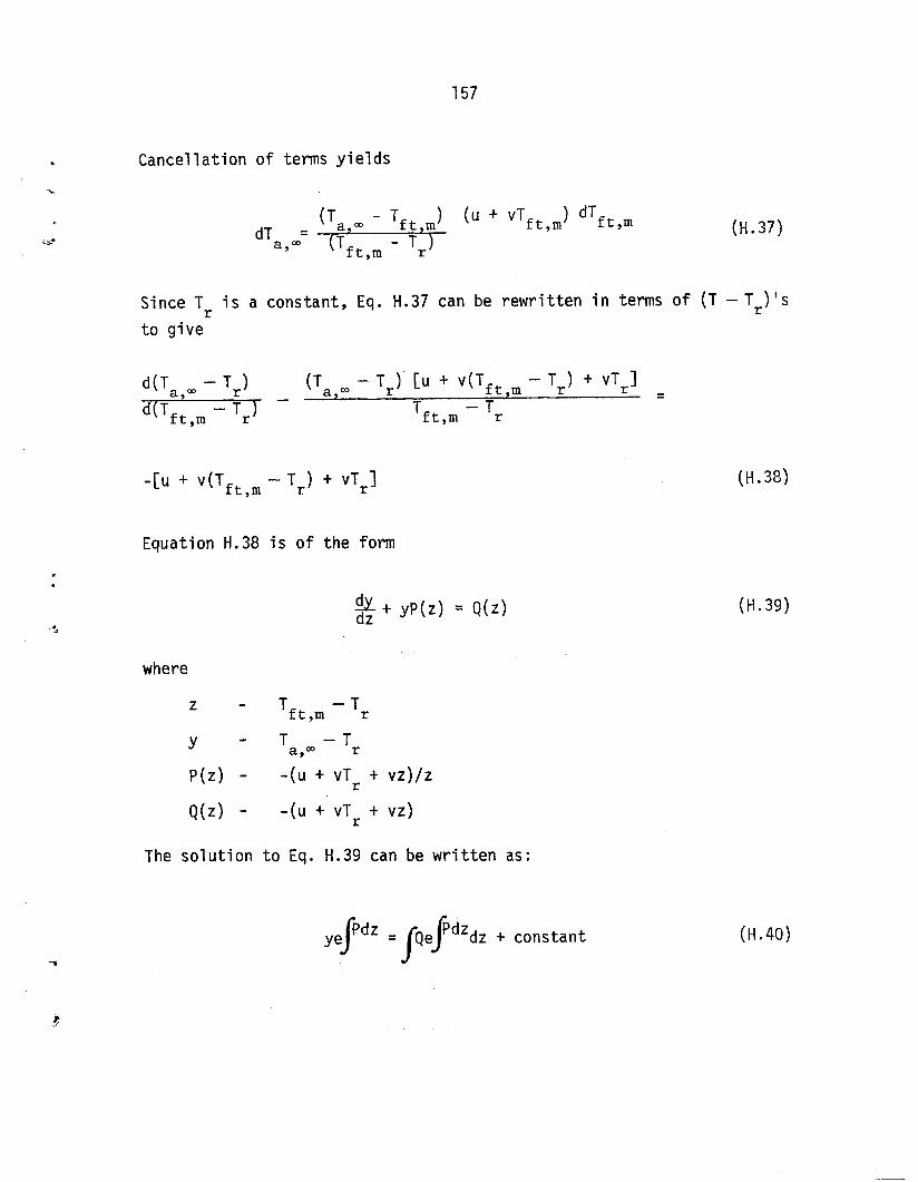
157
Cancellation of terms yields
(Ta,m - Tft,m) (' + VTft,m) dTft,m dTa,coz (T
ft,m r) - T
(H.37)
Since Tr is a constant, Eq. H.37 can
to give
be rewritten in terms of (T - Tr)'s
d(T, a3 - Tr) , (Tap2 - Tr) Cu + v(Tft m - Tr) + vTrl , = d(T -T ) - T -T
ft,m r ft,m r
-[u + v(Tft m - Tr) + vTrl ,
Equation H.38 is of the form
+j$ + YPW = Q(z)
where
' - Tft meTr ,
p(z) - ‘(U + VTr + vz)/z
Q(z) - ‘(U + VTr + vz)
The solution to Eq. H.39 can be written as:
yefdz =pefdzdz t constant
(H.38)
(H.39)
(H.40)

158 -
Evaluating the innermost integral,
1 Pdz = - 1
(u + vTr + vz)dz , and
2
1 Pdz = - [(u + vTr)ln(z)+vt] (H.41)
Then
z- (u + vT,),vz
Next, the outer integral becomes
./
1J Qe PdZdz = - J
(w + vz)z-' eBVZ dz
(H.42)
(H.43)
(H.44)

159
Substitution of Eq. H.45 into Eq. H.44 yields an integrable form, with
the result
f Pdz
f Qe
wz(w
v 2-w + ( "z(3'w)
3-w + 1
V2
(
wz(3'w) vz(4-w)
2! 3-w + 4-w - >
V3
i
wz(4-w)
3-r 4-w +
vz(w 5 -w + --a
)
Equation H.46 can be written in summation form as
i=l
(~.46)
(H.47)
where 'In" is the number of terms which gives acceptable convergence of
the series expansion solution. Substituting Eq. H.47 and H.42 into Eq.
H.40 gives
y(z-’ eevz) = t ,,C(i+U - WI
(i + 1) -w) + C (H.48)
i=l
Equation H.48 can be written in shorthand form as
YF#) = F&z) + C (H.49)

160
The known conditions at the beginning of the dehumidification region are
used to evaluate the constant C in Eq. H.49, i.e.,
.
i
c = yi F1(zi) - F2(zi) (H.50) '.
Use of Eq. H.50 in Eq. H.49 yields the solution for the exit conditions,
y. = ,&--r [FP (‘0) ’ Yi Fl(Zi) - F2(zi)l
Expanding z and y back to their original representations yields
(H.51)
Ta,co(Xo) - Tr = fd ) - T 1 ft,m 0 r'
F CT 2 ft,m('o) -Trl + *
CT,, (Xi) - ‘,I ‘1(‘ft,m(~i’ - ‘r) - ‘2(‘Ft m ,
(x ) -T,)> (H.52) ' i L?
Once T (x ) has been evaluated from Eq. H.52, the humidity ratio of
the exTiaairoW a,m
is calculated from the equation
Wa,,(xo) = pa,&,, - cpTa ,(xo)]/[1061.2 + 0.444*Ta,,.Jx ,] , 0
(H.53)
The sensible heat transfer rate 4, and the rate of water condensation on
the coil, m ,
values of TW
are obtained from Eqs. H.54 and H.55, using the computed
a,m (x0) and Wa,- (x0):
and
4 (H.54) y
-5 2
ri =1;1 W a [wa,co'xi) - wa,co(xo3 (H.55)

161
. The calculations described in this appendix are performed in the
heat pump model only for the region of the coil where the refrigerant is
in a two-phase state. If a fraction of the coil contains superheated
refrigerant vapor, the air flow rate ia is multiplied by f , the fraction
of the coil in a two-phase state, for use in the calculati% of the heat
transfer rates and exit air conditions in the two-phase region.
References for Appendix H
H.l
H.2
H.3
. l
H.4
L F
H.5
H.6
H l 7
H.8
H.9
W. Goodman, "Dehumidification of Air with Coils," Ref'igemrting Engineering, October, 1936, p. 225-274.
J. McElgin and D. C. Wiley, "Calculation of Coil Surface Areas for Air Cooling and Dehumidification," Heating, Piping, and Air Conditioning, March, 1940, pp. 195-201.
C. C. Hiller and L. R. Glicksman, Improving Heat Pwnp Performance via Compressor Capacity Control - AnuZysis and Test, Report No. 24525-96, Heat Transfer Laboratory, Massachusetts Institute of Technology (1976).
J. L. Threlkeld, Thermal Environmental Engineering, Prentice- Hall, Inc., Englewood Cliffs, New Jersey, 1970.
F. C. McQuiston, "Fin Efficiency with Combined Heat and Mass Transfer," ASHRAE Transactions, Vol. 81, Pt. 1, 1975.
F. C. McQuiston and J. D. Parker, Heating, Ventilating, and Air Conditioning Analysis and Design, Wiley, New York, 1977.
R. J. Myers, "The Effect of Dehumidification on the Air Side Heat Transfer Coefficient for a Finned Tube Coil," Master's Thesis, University of Minnesota, 1967.
A. H. Elmahdy and R. C. Biggs, "Performance Simulation of Multi-Row Dry (and/or Wet) Heat Exchangers", Sixth IntemationaZ Heat Tpansfep Conference, Toronto, Aug 7-11, 1978, pp. 327- 332.
N. G. O'Brien and R. L. Turner, "Fin Thermal Efficiency During Simultaneous Heat and Mass Transfer," AICHE Joumal., May 1965, pp. 546-548.
f


1
*-
163
Appendix I - Description of the Dehumidification Algorithm
The calculational scheme used in the moisture removal section of
the evaporator routine (as shown in Fig. 6.4 of the text) is described
in this appendix. The solutions for Tft m (x0) and Ta,,(xo) (the mean
fin-and-tube surface temperature and air'dry bulb temperature,
respectively, at the trailing edge of the evaporator) derived in
Appendix H form the basis for the calculational procedure discussed
here.
A flow diagram of the dehumidification algorithm is shown in Fig.
1.1. The algorithm is used only if the air temperature, Taid, at which
dehumidification would occur at the fin-tube surface is greater than the
exit air temperature T a,m,senS
(x0) from the two-phase region that is
calculated assuming only sensible heat transfer. If this condition
occurs, Taid is then compared to the evaporator inlet air temperature,
T aie' If Taie
is greater than Taid, moisture removal does not occur on
the leading edge of the coil and the fraction of the coil depth which
has only sensible heat transfer, FSenS, is computed from the equation
c w
I
F = en sens [ (Taie - T,)(T,,, - TrJ] 'NtU,tp
Equation I.1 is obtained from the standard effectiveness equation for
Cmin'C max = 0, i.e.,
= 1 - e -N %
tu,tP
by using
T ai,e
-T aid
E= T aie
-T r
(1.1)
(1.2)
0.3)

164
Q a
ORNL-DWG 81-4746~
t1 COMPUTE Cfac (01, 7/w,ft
5 K%~/, f+(O), s(O) s(q) = Sd I
CALCULATE FMOIST
ha,a, (x0), ESTIMATE
Tft ,(x0), COMPUTE I
k; pyo AND SET
L IEIRkJCH = 0 ,
, 4
COMPUTE >
COEFFICIENTS FOR i, FIT
hf+,m , -a +b Tft m+c T2
ft,m
, I \
SOLVE FOR
7 Tft,m “J
c ITERATIVELY I
NO I
COMPUTE hft ,Cx,‘, ho ,(x,J
T~,oD(xb)~Wa,oD(:o),ct~~(~ol,
Fig. I.1 Block Diagram of the Dehumidification Algorithm
I
4

165
1
I
-3.3
and rep1 aci w NtU tp by Fsens N,,, tp. The value of the effective surface
temperature, Tf, i, at the transition point from dry to wet coil, xi, is
equal to the dew'point temperature of the entering air, i.e.,
T ft,m('i) = Tdp a in (1.4) 9 ,
Values for Cfa,(xi), r~,~~(x~), and S(Xi) are computed next. Cfac(X)
is defined by the equation [I.11
wa ,b) - Wft ,b4 'faccx) = T ' '
a,- (x) - T
ft,JXJ l
(1.5)
It follows from Eq. I.4 that when the first part of the coil is dry,
Wa.,(xi) = Wftam(xi) and, from Eq. 1.5, Cfac(xi) = 0.0. It is not
appropriate to-use the wet heat transfer coefficient hw at xi since
dehumidification is just beginning at this point. Were hw used to
replace h at xi, the transition point would shift further into the coil
because of an increase in the effective surface temperature due to the
increase in the air-side heat transfer coefficient. A situation could
occur where moisture removal was predicted when h was used, but not
predicted when Fz~ was used. Thus, h is used at the transition point in
place of kw in the calculation of fin effectiveness nw ft(xi) and the
coil characteristic s(xi). Note that since Cfac(xi) ='0, it follows
from Eq. H.5 that h* = h W W’
Therefore,
T.q,ftcXi) = ~d,ft(Xi) (1.6)
and
s (Xi) = Sd (1.7)
at the transition point.

166
One feature of this procedure needs to be explained before pro-
ceeding to discuss the case where dehumidification occurs at the leading
edge e In the derivation of the solutions for Tft m (x0) and Ta,,(xo)
in Appendix H, the integrations over the coil depth, represented by the
variable "x", were carried out assuming that the coil characteristic s
(and from Eq. H.16, h,, h*w, and nw ft) was constant. That assumption
is handled by using average values &f hw, Jz*~, nw ft, and s over the
region of integration. Local values of these parimeters (at the entrance
and exit of the moisture removal region) as denoted by f(O), f(xi), and
f(xO) are used to obtain the average values and to calculate the local
entrance and exit conditions more exactly.
Returning to Fig. 1.1, when Taid is greater than Tale, dehumidifi-
cation occurs on the leading edge of the coil. In this case, the
temperature at the fin-tube surface T ft m(O) is below the dew point
temperature of the entering air. The vilue of Tft m(O) must be found iteratively using the coil characteristic equation'from Appendix l-l
evaluated at leading edge conditions, i.e.,
T ft,nl(O) - Tr
1 w f&O)
h hw(0) Aft
a, m(O) - hft m(O) , = nw ,+$ i~~-~';c,~~tO), + h c A , , r pm r
which simplified is
s(O) = sw(o>
For the first evaluation of T ft m(OL s(O) is not a-. ,
known because C
and h (0) in Eq. I.8 are not known where C fat(O)
f I3 facto) is given by Eq. I.5 and hfg(0) is given by
I
d
.v-
* *
(1.8) ,'
(I.9
hf,(0) = 1061.2 + 0.444 Tf, I? , )O) + h&N (1.10)
and
I T
hQ(0) = ft,m-32 , if Tft,m 1 32
0 , if T ft,m < 32
(1.11) *

167
The initial evaluation of Tft m(O) is made assuming ,
s(o) = Sd (IJ2)
Equation I.9 is then used with the psychrometric routines [to relate
7-l. ft m(O) to Tft m (0)] to solve iteratively for Tft m(O)a Once an
ini&ial value f& T ft m(O) has been found, Cfac(
are calculated and a Aew value for T
j: hf,(0), and s(O)
ft,m"' is computed. This process
is repeated until the difference in the value of Tft ,(O) from one
iteration to the next is smaller than a prescribed tilerance.
The value of Cfac(0) is then checked to see if it is positive, that
is, to see if the humidity ratio difference from freestream to surface
is positive. If Cfa,(0) is equal to zero, the switch from a dry coil
heat transfer coefficient to a wet coil coefficient [in s(O)] has
caused the surface temperature to rise above the dew point of the
entering air. If such has occurred, the wet coefficient is replaced by
the dry coefficient and the calculation of Tft m(O) is repeated. If
Cfac(o) is not positive at the end of the seco;d series of calculations,
an error message is printed and the program execution is stopped.
Once T ft m(O) has been evaluated at the leading edge of the coil or
) has'been found at the transition point from dry to wet con-
the fraction of the coil depth that is wetted, FmoiSt, and the
of the air at the transition point, h ,(x,), are evaluated.
idification occurs at the leading edge~'fmoist = 1 and xi = 0.
T (x ft,m i ditions,
enthalpy
If dehum
The
T ft,mtx)
coefficients for the quadratic fit of hft ,(x) as a function of
(as assumed in Appendix H) can be estimat;d once the initial
conditions at the start of the dehumidification region have been obtained.
The coefficients are determined using T ft,m('i" an estimate of T
ft rn"o' CT ft m(xi) - 51, and an equation relating hft m to Tft m and Wft ,,'i.e.,
, , , J
h ft,m(~) = 0.24Tft,,(x) + Wf,,,(x) LlC61.2 + O*444Tft,m(x)] (1.13)

168 -'
The saturation curve on the standard ASHRAE psychrometric chart represents
W ft m as a function of Tft m.
by i quadratic equation;
This curve is most closely approximated
hiwever, we will assume that a linear equation .
derived from T ft m(xi) and Tft m(xO) will be adequate, i.e., d
, , . @ .
W ft,m(x) = a' + b'Tft,,(x) (1.14)
where
a' =W ft,m(xi) - b" Tft,m(Xj,) (1.15)
and
b'= [W ft,mo(i) - Wft,m(Xo)l'CTft m('i) - Tft,m(Xo)l (1.16) ,
Substitution of Eq. I.14 into Eq. I.13 yields
h ft,mb) = a + b Tft,mb) + c T:t,mb)
where
a = 1061.2 a'
b = 0.24 + 1061.2 b' + 0.444 a'
C = 0.444 b'
(1.17)
(1.18)
(1.19)
(1.20)
Note that the assumption of
h ft,mtx)
= a* + b*T ft,mcx) (1.21)
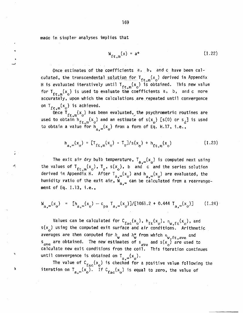
169
made in simpler analyses implies that
1
t 4
w ft,m(x) = a* (1.22)
Once estimates of the coefficients a, b, and c have been cal-
culated, the transcendental solution for Tft m(~o) derived in Appendix a.., .,.. "~, " ̂ . *_ ",
H is evaluated iteratively until Tf, m(xo) ig obtained. This new value
for T ft ,JXo)
is used to evaluate thk coefficients a, b, and c more
accurately, upon which the calculations are repeated until convergence
on T ft ,I& xo) is achieved.
Once T ft m(~o) has been evaluated,/the psychrometric routines are
used to obtai; h ft m(xO) and an estimate of s(xo) [s(O) or sd] is used
to obtain a value +or h a,
co(xo) from a form of Eq. H.17, i.e.,
ha/&) = Uft,m(xO) - T,l/s(xo) + hft,m(xo) (X.23)
i -*
The exit air dry bulb temperature, Ta,,(xo) is computed next using
the values of T ft lnW~ Tr' s(xO), b and c and the series solution
derived in Appendix H. After Ta mu and h,,,(xd) are evaluated, the
humidity ratio of the exit air, ia,_ can be calculated from a rearrange-
ment of Eq. 1.13, i.e.,
‘a ,m(‘c)) = ba,,(xo) - cpa -&,ho)l/Wj~.2 + 0.444 Ta,Jxo)l (L24)
t
'1 -_
Values can be calculated for Cfac(~o)9 hft(x,), T-I, ft(xo), and
s(xO) using the computed exit surface and air condition:. Arithmetic
averages are then computed for hW and ?z; from which nW ft ave and
S ave are obtained. The new estimates of s ave and s(xdi aie used to
calculate new exit conditions from the coil. This iteration continues
until convergence is obtained on T co(xO).
The value of Cfac(xo) is checakid for a positive value following the
iteration on T a,
,(x0). If Cfac(xO) is equal to zero, the value of

I
170 -
J?.Jxd) is set equal to h and the iterations repeated starting at the
solution of T ft m(~O)m Such a situation might occur if dehumidification
bega"ns near the'trailing edge of the coil where the discrete jump
from h to k,(x,) could cause the wet region to revert to a dry surface.
Upon completion of the calculation of the exit air conditions, the
sensible and latent heat transfer rates and the water removal rate in
the two-phase region of the evaporator are computed as described in
Appendix Ma
References “for Appendix I
6.1 F. C. McQuiston, "'Fin Efficiency with Combined Heat and Mass Transfer," ASHRAE Transactions, Vol. 81, Pt. 1, 1975.

171
* Appendix J - Ratios of Geometric Parameters Used in the Heat Exchanger
Calculations
. -4
The correlations for pressure drops and heat transfer coefficients
make use of ratios of air- and refrigerant-side geometric parameters.
The need for and use of these terms is discussed elsewhere and is not
repeated here. This section is-devoted to deriving how these parameters
are calculated; in many instances the equations used are not altogether
straightforward, and they were obtained by various degrees of algebraic
manipulations and cancellation of terms, The input data required for
each heat exchanger:
A - cross-sectional area,
NT - number of tubes In the direction of ajr-flow (horizontally),
*
I* c
N eLircl.lit
*= number of equivalent, parallel refrigerant c'ircujts,
vertical distance between tubes (center-to-center),
wT D a
D r
FP 6 fin thickness,
are suff
However9
as input
icient to describe the evaporator and condenser completely,
there are some basic geometric parameters that are not required
nor explicitly calculated: (see Fig. J.1)
h
e
d
height of the heat exchanger
length of the heat exchanger
depth of the heat exchanger
number of tubes in a row (vertically) N V
horizontal distance between tubes (center-to-center),
outer, or air-side, diameter of tubes,
inner, or refrigerant-side, diameter of tubes,
fin pitch, and
c These remaining basic parameters are not computed because all of the
geometry-related ratios can be computed by careful use of the given

172
h
--_
I w I I I J-1
I I
Fig. J.l Sample Tube-and-Fin Heat Exchanger

173
input parameters. The following equations are used to compute the
geometric ratios used in the Design Model.
N, = number of fins
N,=R Fp
N = tot total number of refrigerant tubes
N tot
= NvNT
d = NT!!,
h = NV s,
V hx = volume of heat exchanger
V hx = lhd = ~(NVST)(NTWT) = NtotRSTW,
A = side the area of each side of each fin is
A Ntot~Da2 TID ' = hd- =
side N
4 totSTWT - NtotT-
A, = fin heat transfer area,
Af = 2NfAside = 21FFpNtot
(J+U
(J-2)
(J-3)
CJ.4)
(J-5)
(5.6)
(J-7)

.
174
A = contact contact area between fins and tubes
A = a
Atubes
A contact = NN
f totnDaS = XFpNtOtnDa6 (5.8)
total air-side heat transfer area
A a =A,+A
tubes
= area of exposed tube surfaces
A =N tu'bes totnDa ' exposed '
,where l exposed is the length of each tube not covered by fins, which can
be written using Eq. J.l:
& exposed = 1 - Nfcs = L(1 - Fp6)
rrD ' A = 2N
a tot~Fp~S,W, - -+I + NtotD~aR(l - F 6) P
A = r refrigerant-side heat transfer area
A r = NtotRIID
r
(J 09)
(J.10)
A free-flow = free-flow frontal area
A free-flow = A - A*tUbes -A*,
(J.11)

175
where AXtubes = "projected ' area of tubes obstructing air flow
A” tubes = NvDa 'exposed
and using Eq. J-9
A" tubes = NvD, le(l - FpS)
PIQ, = total cross-sectional area of the fins obstructing air-flow
A*f = Nfh6 = RFp"(NVST)
A free-flow = l(NVST) - NVD,R(l - Fps) - R(NVS,)Fp6
= RNV[S, - D,(l - Fp6) - STFpS]
= lNV(S, -- Da)(l - FpS)
The ratios that are needed by the heat pump model are:
fin heat transfer area Af c, = contact area = A
contact
Substituting Eqs. J.l, 5.7, and 5.8
lIDa 2RF Ntot(STWT -4 )
l-IDa2 m,w, - -q-- 1
Cf = =
RF N rrD 6 p tot a
__ riDas
(3.72)
(5.13)

176
= total air-side area A a a
a volume of heat exchanger = V hx
Substituting Eq. J.6 and J.10:
2N llDaL
a = totLF (S,W, ---q-- ) + NtotKDal(l - F 6)
a Ntot%WT
=
2F (S,W, -+ ) + r~D,(l -F 6)
%Jm
a = refrigerant-side heat transfer area
r volume of heat exchanger
Substituting Eq. J.6 and J.11:
N a =
toPD nDr r N ,,pTw; = s,w,
F = fin heat transfer area a total air-side heat transfer area
Substituting 5.7 and J.10:
lIDa
F = 2&F Ntot(S,W, -4 )
a Trn 2 2LN totFp(S,W, - "T ) + N&D
a (1 - F a)
P
(5.14)
c
b
f
(5.15)
(J.16) J
6

177
u I free-flow frontal area
a frontal area
Substituting Eq. 5.4 and 5.12:
A free-flow u = A
(5.17) a
+,(S, - Da)(l - F 6) (ST - Da)(l - F 6) u =
= a R(NvsT) ST
(5.18)
A = refrigerant-side heat transfer area rh number of parallel ci,rcuits
Substituting Eq. J.11 and then Eqs. 5.2 and 5.5:
A N llDrL
A =N r tot (3.19)
rh circuits = N circuits
7 r A
(NAN,) G rrDr N#nDr = N = 'TNcircuits
(5.20)
circuits
A = refrigerant-side heat transfer area
0 mass flow rate of air
A A A +zGA r
0 a a free-flow
Substituting Eqs. 5.2, 5.5, J.11, and 5.17 into 5.21:
A =
( NVNT) ((q) flDr
Q 0 GaAa a
(5.21)

178
A = total air-side heat transfer area
min total free-flow frontal area
A A a min = A free-flow
Note that
(5.22)
A a = ($)A, = '2"ArhNcircuits'
r r
and then substituting Eq. J.. 17 into 5.22:
A = 'aArhNcircuits
min LXrAo a

179
4 APPENDIX K: AVAILABILITY AND DISTRIBUTION OF THE HEAT PUMP MODEL
\
The ORNL Heat Pump Model is available to organizations performing
heat pump research development. It is customarily distributed in the
form of six files on a nine track magnetic tape which consist of:
(1)
(2)
(3)
I (4) 4
I (5) I
(6)
FORTRAN source of the model set up for batch processing on a
computer,
sample input data for the Heat Pump Model,
FORTRAN source of a program to fit a fuction of condensing and
evaporating temperatures to compressor map data (this program
can be used to generate the coefficients required to use the
map-based compressor model described in Section 4.3),
sample input data for the map fitting program in file 3,
FORTRAN source for subroutines that can be used to convert the
batch processing version of the Heat Pump Model in file 1
to an interactive program (some of these subroutines are in
addition to those in file 1 and others are used to replace
subroutines in file 1 that have the same name), and
FORTRAN source for an interactive program that can be used to
set up a file of input data for the batch version of the Heat
Pump Model.
These files are listed in Append
the FORTRAN source files).
ices L-Q (with cross-references of
The tapes are written on an IBM computer and:
e

180
o can be at 800, 1600, or 6250 BPI,
e can be in ASCI,I or EBCDIC, and
e can have either labeled or non-labeled fiies.
After a tape is written it is rewound and the copies of the Heat Pump
Model (file 1) and the compressor map fitting program (ffle 3) that are
on the tape are executed using the appropriate data (files 2 and 4).
The printed listing of the job that generated the tape and the output
from these two computer runs are enclosed when the tape is returned.
People who wish to use the interactive programs need to be aware
that they contain system and installation dependent features. The
logical units used for input and output can vary from one computer
system to another and some of the I/O related subroutines will be different.
It is not difficult to identify these differences and it is left to each
recipient of the programs to do this for himself. I(
The interactive input for the programs in files 5 and 6 is organized B
into seven pages of data. Each page contains related information (e.g., :
compressor data, parameters for the indoor heat exchanger) and is designed
to fit on the screen of a CRT terminal. Examples of these pages are
shown in Table K-1. Each data entry on a page is assigned an item
number and a default value. Data is changed by first specifying which
page it is on and then giving the item number and new value. Once the
user has made changes and is satisfied with the results he can:
e save the data for use with the batch version of the model,
l save the data so that it can be read by the interactive model
to override or replace the default data values, and/or
o execute the Heat Pump Model and get output listed on the
computer terminal.
I i !

181
The user needs to be aware that when he selects from two or more alternatives
0
C
(e.g., map-based or loss-and-efficiency compressor model, type of flow
control device) the last one chosen is what will be used.
The programs that are distributed with the Heat Pump Model are
provided as a convenience to the users of the model. They are not
formally documented although there should be sufficient comments in them
to be understandable.
4
P
.
t

183
Table K.l Sample Pages of Input Data for Interactive Version I of Heat Pwnp Model
c PAGE O-1: COMPRESSOR DATA (EFFICIENCY & LOSS MODEL) GEOMETRY: LOSSES:
I
1. DISPLACEMENT (CU IN) 2. CLEARANCE-VOLUME RATIO
14OTOR: 3. SPEED (RPM) -. 4. OUTPUT AT FULL LOAD (KW)
EFFICIENCIES: 5. MAXIMUM MOTOR 6. ISENTROPIC 7. MECHANICAL
4.520 8. .060
3450. 9. 2.149
.820 10.
.700
.800 11.
NOTES: 1. ITEM 8 OR 9 IS SPECIFIED, NOT BOTH 2. ITEM 10 OR 11 IS SPECIFIED, NOT BOTH
HEAT REJECTION RATE FROM COMPRESSOR SHELL (BTU/HR) 0.0
OR FRACTION OF COMPRESSOR POWER REJECTED FROM THE SHELL -350
HEAT TRANSFER RATE FROM HIGH SIDE TO LOW SIDE (BTU/HR) 300.0
OR FRACTION OF COMPRESSOR POWER TRANSFERED FROM HIGH SIDE TO LOW SIDE .ooo
.
I
3. IF ITEM 4 IS SET TO 0, THE NECESSARY OUTPUT AT FULL LOAD WILL BE CALCULATED AND ITEM 3 IS THE ACTUAL MOTOR SPEED
4. IF ITEM 4 IS NOT 0, ITEM 3 IS THE SYNCHRONOUS MOTOR SPEED AND THE ACTUAL SPEED IS CALCULATED
TYPE "RETURN" TO CONTINUE
PAGE #2: COMPRESSOR DATA (MAP-BASED MODEL) GEOMETRY: LOSSES:
1. DISPLACEMENT (CU IN) 4.520 6. HEAT REJECTION RATE FROM 2. BASE DISPLACEMENT FOR COMPRESSOR SHELL (BTU/HR) 0.0
THEMAP (CU IN) 4.520 MOTOR: 7. FRACTION':F COMPRESSOR POWER
3. RATED SPEED (RPM). 3450. REJECTED FROM SHELL .350 SUPERHEAT AT SHELL INLET:
4. BASE SUPERHEAT FOR MAP (F) 20.00 CURVE FITS FROM COMPRESSOR MAP (AS FUNCTIONS OF CONDENSING & EVAPORATING
TEMPERATURES): 5. POWER CONSUMPTION 8. .REFRIGERANT&SS FLOW RATE
CONDENSING l *2 -1.509E-04 CONDENSING **2 -2.6753-02 CONDENSING 4.089E-02 CONDENSING 4.633E+OO EVAPORATING l *2 -1.3383-04 EVAPORATING l "2 4.7033-02 EVAPORATING 5.8603-04 EVAPORATING 9.64OE+OO CONDENSING*EVAPORATING 3.6383-04 CONDENSING*EVAPORATING -1.8683-02 CONSTANT 9.7593-05 CONSTANT 1.207E-04
'NOTE: 1. ITEM 6 OR 7 IS SPECIFIED, NOT BOTH
TYPE, "RETURN" TO CONTINUE

x. I., (2 . . .\..,a. /. ._ .L ̂ ..“” , .” ..-., . . ” .._.

PAGE #3: INDOOR HEAT EXCHANGER GEOMETRY:
1.. FRONTAL AREA (SQ FT) 3.167 2. NUMBER OF PARALLEL CIRCUITS 3.0 3. NUMBER OF TUBE ROWS 3.0 4. NUMBER OF RETURN BENDS 72.0
FAN - FAN MOTOR: 5. COMBINED EFFICIENCY .200
INLET AIR: 6. FLOW RATE (CFM) 1200.0 7. TEMPERATURE (F) 70.0 8. RELATIVE HUMIDITY .500
TYPE "RETURN" TO CONTINUE
PAGE f4: OUTDOOR HEAT EXCHANGER GEOMETRY;
1. FRONTAL AREA (SQ FT) 5.040 2. NUMBER OF PARALLEL-CIRCUITS 4.0 3. NUMBER OF TUBE ROWS 4. NUMBER OF RETURN BENDS 62::
FAN - FAN MOTOR: 5. COMBINED EFFICIENCY .160
INLET AIR: / 6. FLOW RATE (CFM) 2300.0 7. TEMPERATURE (F) 47.0 8. RELATIVE HUMIDITY .700
FINS: TYPE (1 SMOOTH, 2 WAVY, OR 3 LOUVERED) 2. PITCH (FINS/INCH) 14.0 THICKNESS (IN) .00636 THERMAL CONDUCTIVITY (BTU/HR-FT-F) 128.0 CONTACT CONDUCTANCE (BTU/HR-FT2-F) 30000.
TUBES: 14. O.D. (IN) .400 15. I.D. (IN) -336 16. VERTICAL SPACING (IN) 1 .ooo 17. HORIZONTAL SPACING (IN) 0.875
FINS: 9. TYPE (1 SMOOTH, 2 WAVY,
OR 3 LOUVERED) lo. PITCH‘ (FINS/INCH) 11. THICKNESS (IN) 12. THERMAL CONDUCTIVITY
(BTu/HR-FT-F) 13. CONTACT CONDUCTANCE
(BTU/HR-FT2-F) TUBES:
14. O.D. (IN) 15. I.D. (IN) 16. VERTICAL SPACING (IN) 17. HORIZONTAL SPACING (IN)
2. 14.0
.00636
128.0
30000.
.400 -336
1.000 0.875
NOTES: 1. IF ITEM 85 IS SET TO 0, THE FAN VS STATIC EFFICIENCY CURVE IS USED
WITH A 55% EFFICIENT MOTOR TYPE "RETURN" TO CONTINUE


Table K.1 (continued)
PAGE P5: FLOW CONTROL DEVICE FIXED CONDENSOR SUBCOOLING IS BEING USED
SPECIFIED CONDENSER SUBcooLING:. THERMOSTATIC EXPANSION VALVE: 1. DESIRED SUBCOOLING (F) 45.00 '5. VALVE CAPACITY RATING (TONS) .ooo
STATIC SUPERHEAT (F) 0.0 OR 6. CAPILLARY TUBES: 7.
2. NUMBER OF CAPILLARY TUBES 0 3. CAPILLARY TUBE FLOW
FACTOR 0.000 ;: OR
SHORT-TUBE ORIFICE: 4. DIAMETER OF ORIFICE (IN) .ooooo
OR NOTES:
1. CATEGORIES ARE MUTUALLY EXCLUSIVE, I.E.
RATED OPERATING SUPERHEAT (F) o*o BLEED FACTOR .ooo NOZZLE & TUBE PRESSURE . DROP (1 INCLUDE, 0 EXCLUDE) 0
SPECIFY 1, OR 2 & 3, OR 4, OR5-9
2. IF CONDENSER SUBCOOLING IS SPECIFIED, THE VALUES OF ITEMS 2-9 THAT WOULD PRODUCE THAT LEVEL OF SUBCOOLING ARE COMPUTED
TYPE "RETURN" TO CONTINUE


I ..I ..L.....h*.-.-wU
184
PAGE P6: CONNECTING REFRIGERANT LINES EQUIVALENT
GEOMETRY: FROM: TO: ID (IN) LENGTH (FT) LIQUID LINE INDOOR HX OUTDOOR HX 1. 0.190 2. 30.4
REVERSING VALVE SUCTION LINE COMPRESSOR INLET 3. 0.000 4. 0.0 > DISCHARGE LINE COMPRESSOR OUTLET REVERSING VALVE 5. 0.000 .6. 0.0 VAPOR LINE REVERSING VALVE OUTDOOR HX 7. 0.680 8. 6.0 VAPOR LINE REVERSING VALVE INDOOR HX 9. 0.556 10. 30.4
+
RATES OF HIGH SIDE HEAT LOSSES: RATES OF LOW SIDE HEAT GAINS: 11. FROM DISCHARGE LINE (BTU/HR)2000. 13. IN SUCTION LINE (BTU/HR) 300. 12. FROM LIQUID LINE (BTU/HR) 200.
NOTE: 1.
TYPE
GAIN & LOSSES IN ITEMS 11-13 C!N BE FOR VALIDATION RUNS OR TO SIMULATE HIGH TO LOW SIDE HEAT EXCHANGERS AND REVERSING "RETURN" TO CONTINUE
VALVES
PAGE 1. 2.
3. 4. 5.
6.
#7: MISC. DATA TITLE: HOUSE LOAD AT OUTDOOR AMBIENT (BTU/HR) 15000. EVAPORATOR SUPERHEAT (F) 10.0 DUCT SIZE (IN) 8.0 MODE OF OPERATION (1 COOLING, 2 HEATING) 2 LEVEL OF OUTPUT (0 SUMMARY, 1 COMPRESSOR, 2 COILS, 3 STANDARD) 1
EFFECTS OF HEAT LOSSES ON INLET AIR: 7. INDOOR FAN (SEE NOTE BELOW) 2 '- 8. OUTDOOR FAN (SEE NOTE BELOW) i 9. COMPRESSOR (SEE NOTE BELOW) 1 f ESTIMATES TO BEGIN ITERATIONS: *
10. EVAPORATING TEMPERATURE (F) 30.0 11. CONDENSING TEMPERATURE (F) 115.0 12. REFRIGERANT MASS FLOW
RATE (LBM/HR) 400.0 NOTE:
1. HEAT LOSSES FROM THE FANS AND COMPRESSOR CAN BE ADDED TO THE AIRSTREAM EITHER BEFORE OR AFTER‘IT CROSSES THE COIL (SIMULATE BLOW-THROUGH & DRAW-THROUGH FANS)
THE HEAT LOSS SPECIFY 0 TO NEGLECT 1 TO ADD THE 2 TO ADD' THE
TYPE "RETURN" TO CONTINUE
HEAT To THE AIR BEFORE IT CROSSES THE COIL HEAT To THE AIR AFTER IT CROSSES THE COIL
‘(I
tr


185
J
Appendices L, M, N, 0, P, and Q are on microfiche in an envelope attached
8 to the back cover.
1
; -li .
i
: z r