Gravity inversion of basement relief using approximate equality constraints on depths

GEOPHYSICS, VOL. 62, NO. 6 (NOVEMBER-DECEMBER 1997); P. 1745–1757, 9 FIGS., 4 TABLES.

Gravity inversion of basement relief usingapproximate equality constraints on depths

Valeria Cristina F. Barbosa∗, Joao B. C. Silva∗,and Walter E. Medeiros‡

ABSTRACT

We present a gravity interpretation method for esti-mating the relief of an arbitrary interface separating twohomogeneous media. The upper medium is discretizedinto rectangular, juxtaposed prisms whose thicknessesrepresent the depths to the interface and are the param-eters to be estimated from the gravity anomaly. The den-sity contrast of each prism is assumed to be constant andknown. To stabilize the inversion, we introduce two kindsof constraints on the depths. The first one requires prox-imity between the observed and computed depths at iso-lated points such as those obtained from boreholes (ab-solute equality constraint). The second one requires thatgroups of depths approximately follow an establishedlinear relationship among the depths (relative equalityconstraint). Both kinds of constraints are imposed in theleast-squares sense.

We illustrate the method performance by applying it toa synthetic anomaly produced by a simulated basement

relief consisting of four narrow and adjacent structurallows. Only two structural lows produced isolated gravitylows. Nonetheless, the whole basement topography wassuccessfully reconstructed with an average error of 4% ofthe maximum relief amplitude. In this example, the rela-tive constraints established that the thicknesses of adja-cent prisms should be as close as possible to each other(overall relief smoothness). As absolute constraints weused point information about the basement depth at fivepoints.

In addition to the overall relief smoothness, otherrelevant geologic information, such as localized reliefsmoothness, occurring at structural terraces, for exam-ple, can be incorporated by assigning different weightsto the relative equality constraints.

The method was applied to the gravity anomaly ofReconcavo Basin, Brazil, leading to a sharper definitionof the basement features relative to previous gravity in-terpretations of this area.

INTRODUCTION

Estimating, from the gravity anomaly, the depth to an in-terface separating two contrasting media is a nonlinear in-verse problem. Most methods so far presented for solving thisproblem may be grouped into two categories. Methods in thefirst category do not minimize a stabilizing functional, whereasthose in the second category do, allowing incorporation of apriori information about the sources in a simple fashion.

In the first category, Bott (1960), Tanner (1967), and Cordelland Henderson (1968), for example, assumed that the den-sity contrast 1ρ between the media is known and proposediterative procedures similar to a trial-and-error process imple-mented in an automatic way. In these methods, the solution is

Manuscript received by the Editor April 25, 1996; revised manuscript received January 13, 1997.∗Department Geofısica, CG, Federal University of Para, Caixa Postal 1611, 66.0017-900, Belem, PA, Brazil. E-mail: [email protected].‡Department Fısica/CCE, Federal University of Rio Grande do Norte, Caixa Postal 1641, 59.072-970, Natal, RN, Brazil. E-mail: [email protected]© 1997 Society of Exploration Geophysicists. All rights reserved.

obtained from successive linear approximations for the thick-nesses of the upper medium. Neither the algorithm conver-gence nor the solution stabilization is guaranteed by thesemethods.

Also in the first category are several inverse methods basedon Parker’s (1973) formula to compute the gravity effect of anarbitrary interface separating two homogeneous media, suchas the methods of Oldenburg (1974), Pilkington and Crossley(1986), and Guspı (1993). Because these methods stabilize thesolutions either by applying a low-pass filter to the data or byemploying a damping parameter, they implicitly introduce thea priori information that the interface is smooth. The lowerthe cutoff frequency or the larger the damping parameter, thesmoother the computed interface.

1745

1746 Barbosa et al.

In the second category, a stabilizing functional is minimized,allowing the introduction of different kinds of geologic in-formation. Leao et al. (1995), for example, transformed theBouguer anomaly into a map of depths relative to a referencelevel by downward continuing the anomaly and dividing it bya scale factor involving 1ρ. The functional to be minimized isthe norm of the residuals between the known and computeddepths at isolated points. In addition, the solutions are stabi-lized by a damping parameter in the downward-continuationoperator. Richardson and MacInnes (1989), on the other hand,minimized the weighted norm of the distance between the fi-nal solution and a reference solution (the starting guess) usingthe a priori parameter covariance matrix as a weight. Largerweights are assigned to more reliable depth information (fromboreholes, for example). The final solution, although stable, ishighly biased toward the starting solution. In this case, gooda priori knowledge of the relief must be available.

We present a stable gravity interpretation method for aninterface separating two homogeneous media. The stabilityis attained by introducing approximate relative and absoluteequality constraints (Medeiros and Silva, 1995) on the inter-face depths. The relative equality constraints impose on thesolution either an overall or a local smooth behavior for thespatial parameter distribution (depths to the interface). The ab-solute equality constraints impose the constraint that at pointsat which the depths are known, the computed depths must beas close as possible to the observed depths. These constraintsallow a straightforward and versatile way to introduce a priorigeologic information. For example, by assigning relative equal-ity constraints to a selected group of parameters, informationabout the presence of known basement terraces in a sedimen-tary basin may be incorporated easily. The absolute constraintscontribute in stabilizing the solutions and allowing a smaller de-gree of smoothness to be imposed on the interpreted interface.

The performance of the method was assessed in tests usingsynthetic data with the purpose of mapping a complex inter-face consisting of four structural highs and lows. Despite thefact that the gravity effect of some structural features of thesynthetic basin was not noticeable just by anomaly inspection,the method resolved all structural highs and lows with an av-erage error, for the computed depths relative to the true ones,of 4% of the maximum relief amplitude.

The method was also applied to the Bouguer anomaly ofReconcavo Basin, Brazil, leading to a sharper definition of thebasement features (such as terraces and depocenters) relativeto previous gravity interpretations of this area.

METHODOLOGY

The inverse problem

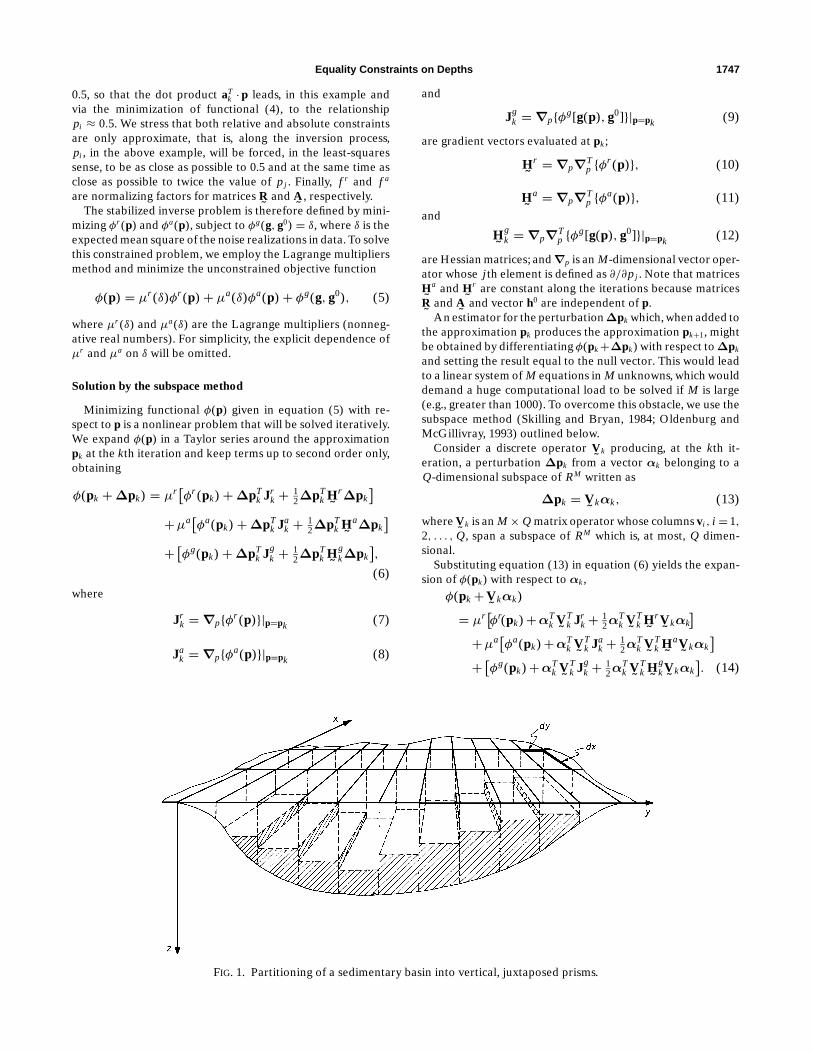
Assume that a sedimentary basin consisting of homogeneoussediments and basement can be modeled by a set of elemen-tary sources. A finite region of the x-y-z space, containing en-tirely the basin, is discretized into M juxtaposed, 3-D prisms(Figure 1) whose tops are at the earth’s surface. The thicknessesof the prisms are the parameters to be estimated from the grav-ity data. We assume that the gravity data are interpolated on aregular grid. For simplicity, the number M of prisms is set equalto the number of points on the grid of observations, and thex- and y-coordinates of the center of the j th prism coincidewith the respective coordinates of the j th observation. Also

for simplicity, we assume that the density contrast between thesediments and the basement is known.

The only parameters to be estimated (the thicknesses of theelementary prisms) are related to the gravity field by the non-linear relationship

gi =M∑

j=1

F(pj , ri ), i = 1, 2, . . . ,M, (1)

where F(pj , r i ) is the nonlinear function (Telford et al., 1976)associating the i th gravity observation to the j th parameterpj (thickness of the j th prism) of the interpretation model,and r i is the position vector of the i th observation in thex-y-z space. The term gi defines the i th element of vectorg ≡ g(p) ≡ {g1, g2, . . . , gM }T containing the computed gravityanomaly, where p ≡ {p1, p2, . . . , pM }T is the vector of param-eters of the interpretation model and the superscript T standsfor transposition.

The nonlinear inverse problem of estimating p ∈ RM from gmay be formulated as the optimization problem of minimizingthe functional

φg(g, g0) = 1M‖g− g0‖2, (2)

where g0 ≡ {g01, g

02, . . . , g

0M }T is the vector containing the grav-

ity observations and ‖·‖ is the Euclidean norm. This problem,however, is ill-posed because its solution is unstable. To trans-form this problem into a well-posed one, we introduce twokinds of constraints: relative and absolute (Medeiros and Silva,1995). The relative constraints establish linear relationshipsamong elements of the parameter vector. The spatial smooth-ness of the parameters is one example of this kind of constraint:it imposes the constraint that adjacent parameters (thicknessesof adjacent prisms) must be close to each other. The absoluteconstraints require that some (or all) elements of the parame-ter vector be closest to some numerical values known a priori,as, for example, values from boreholes. The relative and abso-lute constraints are introduced by minimizing, respectively, thefunctionals

φr (p) = f r

M‖

˜Rp‖2, (3)

and

φa(p) = f a

M‖

Ãp− h0‖2. (4)

Terms˜R,

Ã, and h0 are described below.

˜R is an L × M matrix

whose L lines allow, among other possibilities, establishment ofL a priori linear relationships among pairs of parameters. Forexample, if there is a priori information that the i th parameteris twice as big as the j th parameter, the M-dimensional vectorrl , defining the l th line of matrix

˜R, will be composed of null

elements, except for the i th and j th elements, which will beset to 1 and −2, respectively. As a result, the dot product rT

l ·pleads, in this example and via the minimization of functional(3), to the relationship pi − 2pj ≈ 0.

Ã is an N × M matrix

(N ≤ M) that forces N parameters to be close to N a prioriknown numerical values h0. For example, if we have the infor-mation that the i th parameter must be close to 0.5, then thekth row of

Ã will be the M-dimensional vector ak, composed

of null elements, with the exception of the i th element, whichwill be equal to 1. Accordingly, the kth element of h0 will be

Equality Constraints on Depths 1747

0.5, so that the dot product aTk ·p leads, in this example and

via the minimization of functional (4), to the relationshippi ≈ 0.5. We stress that both relative and absolute constraintsare only approximate, that is, along the inversion process,pi , in the above example, will be forced, in the least-squaressense, to be as close as possible to 0.5 and at the same time asclose as possible to twice the value of pj . Finally, f r and f a

are normalizing factors for matrices˜R and

˜A, respectively.

The stabilized inverse problem is therefore defined by mini-mizing φr (p) and φa(p), subject to φg(g, g0) = δ, where δ is theexpected mean square of the noise realizations in data. To solvethis constrained problem, we employ the Lagrange multipliersmethod and minimize the unconstrained objective function

φ(p) = µr (δ)φr (p)+ µa(δ)φa(p)+ φg(g, g0), (5)

where µr (δ) and µa(δ) are the Lagrange multipliers (nonneg-ative real numbers). For simplicity, the explicit dependence ofµr and µa on δ will be omitted.

Solution by the subspace method

Minimizing functional φ(p) given in equation (5) with re-spect to p is a nonlinear problem that will be solved iteratively.We expand φ(p) in a Taylor series around the approximationpk at the kth iteration and keep terms up to second order only,obtaining

φ(pk +∆pk) = µr[φr (pk)+∆pT

k Jrk + 1

2∆pTk ˜

Hr ∆pk]

+µa[φa(pk)+∆pT

k Jak + 1

2∆pTk ˜

Ha∆pk]

+ [φg(pk)+∆pTk Jg

k + 12∆pT

k ˜Hg

k∆pk],

(6)

where

Jrk =∇p{φr (p)}|p=pk (7)

Jak =∇p{φa(p)}|p=pk (8)

FIG. 1. Partitioning of a sedimentary basin into vertical, juxtaposed prisms.

and

Jgk =∇p{φg[g(p), g0]}|p=pk (9)

are gradient vectors evaluated at pk;

˜Hr =∇p∇T

p {φr (p)}, (10)

˜Ha =∇p∇T

p {φa(p)}, (11)and

˜Hg

k =∇p∇Tp {φg[g(p), g0]}|p=pk (12)

are Hessian matrices; and∇p is an M-dimensional vector oper-ator whose j th element is defined as ∂/∂pj . Note that matrices

˜Ha and

˜Hr are constant along the iterations because matrices

˜R and

˜A and vector h0 are independent of p.

An estimator for the perturbation ∆pk which, when added tothe approximation pk produces the approximation pk+1, mightbe obtained by differentiating φ(pk+∆pk) with respect to ∆pk

and setting the result equal to the null vector. This would leadto a linear system of M equations in M unknowns, which woulddemand a huge computational load to be solved if M is large(e.g., greater than 1000). To overcome this obstacle, we use thesubspace method (Skilling and Bryan, 1984; Oldenburg andMcGillivray, 1993) outlined below.

Consider a discrete operator˜Vk producing, at the kth it-

eration, a perturbation ∆pk from a vector αk belonging to aQ-dimensional subspace of RM written as

∆pk =˜Vkαk, (13)

where˜Vk is an M × Q matrix operator whose columns vi , i = 1,

2, . . . , Q, span a subspace of RM which is, at most, Q dimen-sional.

Substituting equation (13) in equation (6) yields the expan-sion of φ(pk) with respect to αk,

φ(pk+˜Vkαk)

= µr[φr(pk)+αT

k ˜VT

k Jrk+ 1

2αTk ˜

VTk ˜

Hr

˜Vkαk

]+µa

[φa(pk)+αT

k ˜VT

k Jak + 1

2αTk ˜

VTk ˜

Ha

˜Vkαk

]+ [φg(pk)+αT

k ˜VT

k Jgk + 1

2αTk ˜

VTk ˜

Hgk ˜Vkαk

]. (14)

1748 Barbosa et al.

Differentiating equation (14) with respect toαk and equatingthe result to the null vector, we obtain the normal equation forthe estimate α∗k, which is

˜VT

k

(µr

˜Hr + µa

˜Ha +

˜Hg

k

)˜Vkα

∗k

= −˜VT

k

(µr Jr

k + µaJak + Jg

k

). (15)

From now on, we use “*” to distinguish estimates from true pa-rameters. Equation (15) represents a system of Q linear equa-tions in Q unknowns, which requires much less computationaleffort (if Q¿ M) than the original problem: solving a systemof M linear equations in M unknowns.

The original problem of estimating, at the kth iteration, vec-tor p∗k+1 which minimizes the functional given in equation (5)was, therefore, transformed into the problem of estimating αk

and ∆pk with equations (15) and (13), respectively.

Selecting the subspace

Given an M-dimensional parameter space RM , there will bemany Q-dimensional subspaces of RM . A particular subspace isconsidered adequate for iteratively solving a nonlinear inverseproblem if, at every iteration, the estimate α∗k leads to a step∆p∗k that efficiently decreases the objective function φ(p∗k). Atthe first iterations, when p∗k is far from the minimum, functionφ(p∗k) is rapidly decreased by moving p∗k along the gradient ofφg(p∗k). However, close to the solution, the gradient of φg(p∗k)becomes very low because of the ambiguity of the geophys-ical inverse problem. At this stage, further improvements indecreasing φ(p∗k) can be achieved only by moving p∗k along thegradients of φr (p∗k) and φa(p∗k). Thus, we defined a subspaceRQ by selecting Q−2 vectors associated with functional φg(p),one vector associated with functional φr (p), and one vectorassociated with functional φa(p).

The Q−2 vectors associated with φg(p) are obtained by par-titioning the set of M observations into Q− 2 disjoint subsets.The fitting functional φg(p) is likewise partitioned into Q − 2subsets as

φg(p) =Q−2∑m=1

φgm(p), (16)

where the functional φgm(p), belonging to the mth subset, is

defined as

φgm(p) = 1

M

∥∥gm − g0m

∥∥2, (17)

and g0m and gm contain, respectively, the observed and com-

puted gravity data, belonging to the mth subset. In this way,each subset of φg(p) contains information about one particularsubset of the M observed (and computed) data. The gradient∇p{φg

m(p)}|p=pk defines the mth column vector vm of matrix˜Vk.

Vectors associated with functionalsφr (p) andφa(p) composethe last two columns of Vk and are defined as

vQ−1 = ∇p{φr (p)}|p=pk (18)

and

vQ = ∇p{φa(p)}|p=pk . (19)

We stress that the definition of vectors vm,m = 1, 2, . . . , Q,given above does not guarantee their linear independence.

Therefore, these vectors span a space that is at most Q di-mensional. If vectors vm are linearly dependent, another set ofvectors (or another value for Q) should be selected because inthis case, the solution of equation (15) is not unique. However,we never encountered such a situation, even when assumingvalues of Q as small as one-tenth M .

Computational details

At the kth iteration,αk is estimated by solving the linear sys-tem of equations (15). When the approximation p∗k lies outsidethe region in which the quadratic expansion of φ(p∗k) is valid,the computed step ∆p∗k may lead to an approximation p∗k+1 pro-ducing a larger objective function value than p∗k, thus prevent-ing the algorithm convergence. To overcome this difficulty, weused the nonlinear optimization method of Marquardt (1963)by adding, at each iteration, a positive number λk to the diag-onal of matrix

˜B = (µr

˜Hr +µa

˜Ha+

˜Hg

k) in equation (15). Thisnumber is initialized with a value of 1% of the largest singularvalue of

˜B. To reduce the computational load, we employed

the Gauss-Newton approximation of the Hessian matrix˜Hg

k .The normalizing factors f r and f a in equations (3) and (4),

respectively, are defined at each iteration as

f rk =

Egk

Erand f a

k =Eg

k

Ea, (20)

where Egk , Er , and Ea are the Euclidean norms of

˜Hg

k, ˜Hr , and

˜Ha, respectively.

The iteration is stopped when the following inequality is sat-isfied: ∣∣∣∣∣φ

(p∗k−1

)− φ(p∗k)φ(p∗k) ∣∣∣∣∣ ≤ ε, (21)

where ε is a threshold below which the relative decay of φ(p)is assumed to be constant. In this paper, we use ε = 0.1. Notethat the stopping criterion is defined with respect to the func-tional φ(p) given in equation (5) and not with respect to thedata-fitting functional φg(p) given in equation (2). This choiceensures the incorporation of the constraints on parameters inaddition to fitting the geophysical observations.

Factors µr and µa in equation (5) express, respectively, therelative importance of φr (p) and φa(p) with respect to φg(p),that is, µr and µa reflect the interpreter’s reliability on the apriori information incorporated by the relative and absoluteconstraints, with respect to the geophysical information. Theinterpreter must select values for µa and µr that produce thelargest ratio µa/µr , additionally satisfying the constraints that(1) the observations must be explained within the experimentalerrors, (2) the solution must be stable, and (3) the solutionshould not present pinnacles around the points associated withthe absolute constraints. The presence of pinnacles indicatesa conflict between the absolute and the relative constraintsproduced by the simultaneous requirements that the relief besmooth and pass through the points of known depths.

SYNTHETIC EXAMPLE

Figure 2 shows the contoured relief of a synthetic sedimen-tary basin compounded by an array of 33 × 26 juxtaposedprisms with dimensions of 1 km in both x- and y-directions(north-south and east-west, respectively). The thicknesses of


the prisms represent the depths to the basement, and a con-stant density contrast of−0.2 g/cm3 was assigned to all prisms.The theoretical gravity anomaly was computed on a plane at50 cm above the surface. The horizontal coordinates of the ob-servations coincide with the coordinates of the centers of theprisms. Pseudorandom Gaussian noise with zero mean and astandard deviation of 0.1 mGal was added to the theoreticalanomaly, producing the simulated anomaly shown in Figure 3(solid lines).

The basin presents four northwest-trending subbasins (A–Din Figure 2). Nonetheless, this structural framework is by nomeans reflected in the gravity anomaly of Figure 3, which shows

FIG. 2. Synthetic example. True basement relief of a complex sedimentary basin. P1–P5 locate the positions ofsimulated boreholes that intersected the basement. The contour interval is 0.5 km.

two isolated lows (B1 and D1) but no isolated highs. The onlyevidence of the existence of subbasin C is the deflection ofthe isovalue curves toward the northeast around point C1 inFigure 3. Thus, a qualitative inspection of Figure 3 might in-dicate a possible northeast-trending structural low betweenB1 and D1. Although the gravity low B1 coincides with struc-tural low B, the gravity low D1 lies between structural high H(Figure 2) and structural low D. Finally, the very existence ofsubbasin A might, at most, be guessed from the subtle distor-tion of the gravity isovalue curves at A1 (Figure 3).

We used an interpretation model identical to the truemodel described above. Absolute equality constraints, at five

1750 Barbosa et al.

points (P1–P5 in Figure 2) where the depth to the basement isassumed to be known from boreholes, were incorporated usinga value of µa = 1 in equation (15). The x- and y-coordinates ofthese wells, as well as the corresponding basement depths, areshown in Table 1. To illustrate the effectiveness of the relativeequality constraints, even when a basin structural frameworkwas poorly known, we used a matrix

˜R whose rows contain just

two nonnull elements: 1 and−1. Minimizing φr (p) leads, there-fore, to equations of the form pi ≈ pj , for all i and j valuescorresponding to adjacent prisms. We set the factor µr to the

FIG. 3. Synthetic example. Noise-corrupted Bouguer anomaly produced by the simulated sedimentary basin ofFigure 2 with a density contrast of−0.2 g/cm3. P1–P5 locate the positions of simulated boreholes that intersectedthe basement. The contour interval is 1 mGal.

Table 1. Synthetic example: x- and y-coordinates of the fiveboreholes, P1–P5, in Figure 2 and the corresponding depths tothe basement.

x-coordinate y-coordinate Depth to the basementBorehole (km) (km) (km)

P1 21.0 10.0 2.0P2 28.0 20.0 2.5P3 28.0 2.0 2.0P4 4.0 23.0 1.0P5 29.0 9.0 0.5


smallest positive value, still producing geologically meaningfulsolutions (0.001 in this test). In applying the subspace method,we partitioned the data set into 85 nonoverlapping subsets often observations and one subset of eight observations arrangedin the following way. Starting at the northwestern corner, thefirst subset consists of the first ten observations located in thenorthernmost row of observations. The second subset includesthe next ten observations in the same row, and so on, untilthe first row of data is completely covered. Then, we moveto the adjacent row on the south and resume the procedure. Thestarting solution was obtained by assigning to every elementaryprism the thickness of a Bouguer slab reproducing the gravityanomaly value just above the prism center.

FIG. 4. Synthetic example. Basement relief estimated by the proposed method usingµr = 0.001 andµa= 1. P1–P5locate the positions of simulated boreholes that intersected the basement. The contour interval is 0.5 km.

The results of the method are shown in Figure 4. Eleven iter-ations were necessary to attain the convergence criterion usinga value of 0.1 for constant ε in equation (21). Despite the in-evitable loss of resolution required to stabilize the solution, theestimated basement surface determines the horizontal positionand extension of all four subbasins and, consequently, the highsseparating them. Figure 5 shows the absolute differences be-tween the true and estimated basement reliefs. For most of thearea, this difference is smaller than 0.5 km, corresponding toabout 7% of the maximum relief amplitude. Larger differences(up to 1.25 km, corresponding to 18% of the maximum ampli-tude) coincide mainly with the subbasins having the steepestborders and the narrowest bottoms (B and D in Figure 2). Note

1752 Barbosa et al.

that over the structural highs, which are particularly importantin oil prospecting, the residuals are small. Figure 3 shows thefitted gravity anomaly (dashed lines), and Table 2 displaysthe observed and estimated depths at the borehole locations.The root-mean-square of the absolute differences between theobserved and estimated depths is 0.037 km.

To evaluate the importance of the absolute constraints, werepeated the above-described inversion using just the rela-tive equality constraints. The results (Figure 6) show that thebottom extent of subbasin B along the northwest direction is

FIG. 5. Synthetic example. Absolute differences between the true (Figure 2) and the estimated (Figure 4) base-ment reliefs. The contour interval is 0.25 km.

Table 2. Synthetic example: observed and estimated depthsat the five boreholes, A–E, in Figure 2.

Observed depth Estimated depthBorehole (km) (km)

P1 2.00 1.96P2 2.50 2.47P3 2.00 2.00P4 1.00 1.04P5 0.50 0.45


now slightly underestimated. The bottom of subbasin C showsa lower resolution: it presents a flat and uniform aspect, incontrast with the results obtained using absolute constraints,which permitted inference of the presence of the lows labeledJ and L in Figure 2 not only from the presence of the 4.5-kmisovalue curve at J (Figure 4) but also from the narrowing of the4-km isovalue curve at K. The above-mentioned differences aresubtle. However, we stress that this is a conservative situationbecause the boreholes were located at random. In a real situa-tion, boreholes are expected to be located inside the closuresof the structural lows, constraining, in this way, the estimatedrelief in a more dramatic way, as was in fact confirmed withsynthetic examples (not shown).

FIG. 6. Synthetic example. Basement relief estimated by the proposed method usingµr = 0.001 andµa= 0.0. Thecontour interval is 0.5 km.

For the purpose of comparison, in Figure 7 we show the inver-sion of the gravity anomaly of Figure 3 using Leao et al.’s (1995)method. The simulated boreholes (W1–W5 in Figure 7) coin-cide with the deepest points of the subbasins. The boreholesare different intentionally from the ones shown in the previoustest. Here, the selected borehole positions are optimum be-cause the deepest point of a basin usually is poorly resolved bythe gravity data. Comparing Figures 4 and 7, we note the greaterability of the proposed method in defining the basement reliefeven with a poor choice of borehole locations. The smooth-ing observed in Figure 7 follows from the fact that in Leaoet al.’s (1995) method, the computed interface is approximated(within a multiplicative constant) by the downward-continued

1754 Barbosa et al.

gravity anomaly. Therefore, an additional assumption aboutthe interface is implicitly introduced; that is, it is a continuoussurface having first- and second-order continuous derivatives.

REAL DATA APPLICATION

The proposed method was applied to the gravity anomalyof Reconcavo Basin, Brazil. This basin developed from an Up-per Jurassic to Lower Cretaceous rupture feature implantedover terrains of different natures and ages. The origin of thisrift is related to the breakup of Gondwana and the open-ing of the South Atlantic Ocean. The sedimentary cover in

FIG. 7. Synthetic example. Basement relief estimated by Leao et al.’s (1995) method. W1–W5 locate the positionsof simulated boreholes that intersected the basement. The contour interval is 0.2 km.

the Reconcavo Basin comprises rocks from Upper Jurassic toTertiary periods and locally may be 6 km thick (Milani andDavison, 1988). The basement is segmented by severalnortheast- and northwest-trending normal faults.

Figure 8 shows the Bouguer gravity anomaly (solid lines) re-sulting from the topography of the basement obtained by Leaoet al. (1995). We used a grid spacing of 3 km in both north-southand east-west directions. To apply the subspace method, we par-titioned the set of 889 gravity observations into 88 nonoverlap-ping subsets containing 10 observations and 1 subset containing9 observations. The same procedure described for the syntheticexample was used here to produce the subsets.


The thickness of the sediments is known at seven isolatedpoints where boreholes touched the basement (A–G inFigure 8). These depths were used as absolute constraintsby assigning a value of 0.5 to factor µa in equation (15).The borehole locations and the corresponding depths tothe basement are shown in Table 3. In addition, relativeequality constraints were incorporated by using a matrix

˜R

similar to the one employed in the synthetic example, so thatan overall smoothness is imposed on the basement relief.Factor µr was assigned a value of 0.5. Smaller values of µr

produced pinnacles in the estimated relief around the bore-holes, indicating a possible inconsistency between the borehole

FIG. 8. Reconcavo Basin, Brazil. Bouguer anomaly produced by the basement relief, according to Leao et al.(1995). The contour interval is 2 mGal.

Table 3. Reconcavo Basin: geographic coordinates of theseven boreholes, A–G, in Figure 8 and the correspondingdepths to the basement.

DepthBorehole Latitude Longitude (km)

A 12◦ 01′ 26.4′′ S 37◦ 59′ 16.8′′W 2.29B 12◦ 19′ 54.9′′ S 38◦ 14′ 42.6′′W 2.88C 12◦ 47′ 34.8′′ S 38◦ 26′ 45.6′′W 3.80D 12◦ 08′ 09.6′′ S 38◦ 11′ 08.5′′W 2.95E 12◦ 15′ 09.6′′ S 38◦ 04′ 15.2′′W 1.62F 12◦ 10′ 08.4′′ S 38◦ 12′ 27.7′′W 2.97G 12◦ 11′ 20.4′′ S 38◦ 13′ 19.2′′W 3.14

1756 Barbosa et al.

information and the gravity data, probably caused by an unre-moved base level in the data. We performed several inversionsassuming different density contrast values in the −0.25 g/cm3

to −0.46 g/cm3 range and selected the value −0.26 g/cm3 onthe basis of the norm of the differences between the knownand computed depths at points A–G. The same convergencecriterion employed in the synthetic example was adopted, andthe starting solution was obtained in the same way as in thesynthetic example.

The estimated basement relief is shown in Figure 9, andthe fitted gravity anomaly is shown in Figure 8 (dashed lines).Some known structural features are apparent in Figure 9. TheAlagoinhas (T), Camacari (U), and Quiambina (Q) structurallows coincide with three lows in Figure 9. Low gradientareas coincide with the Cassarongongo, Sao Domingos, and

FIG. 9. Reconcavo Basin, Brazil. Relief estimated by the proposed method using µr = 0.5 and µa= 0.5. Thecontour interval is 0.25 km.

Mata-Aracas terraces (V, SD, and MA, respectively) andthe Miranga structural low (MI). The presence of a newnortheast-trending terrace is inferred from the low gradientarea limited by the isovalue curves of 2.5 and 3.5 km aroundstructural low MI. This terrace, together with the Mata-Aracasterraces, isolates the main structural low (Alagoinhas) fromthe basin depocenter (Camacari). These results are consistentwith the interpretation that the basement of the ReconcavoBasin consists of a mosaic of normally faulted blocks. Thedefinition of the terraces around the two major structural lows(Alagoinhas and Camacari) was possible because of the goodresolution attainable with the proposed method.

Table 4 shows the observed and computed basement depthsand the absolute differences between them at boreholes A–G.The fitted Bouguer anomaly is shown in Figure 8 (dashed lines).


Table 4. Reconcavo Basin: observed and estimated basementdepths and the difference between them at seven boreholes.

Observed depth Estimated depth DifferenceBorehole (km) (km) (km)

A 2.29 2.09 0.20B 2.88 2.91 0.03C 3.80 3.26 0.54D 2.95 3.38 0.43E 1.62 1.56 0.06F 2.97 3.33 0.36G 3.14 3.35 0.21

CONCLUSIONS

We presented a gravity interpretation method for mappingthe relief of a sedimentary basin. The method is stabilized byincorporating approximate absolute and relative equality con-straints on the depths to the basement. The problem is non-linear and solved iteratively by Marquardt’s (1963) method,modified to incorporate the subspace method, which typicallyreduces by one order of magnitude the dimension of the linearsystem of equations to be solved at each iteration.

As compared with methods designed for the same purpose,the proposed method provides an improved resolution becausethe a priori information introduced to stabilize it does not im-plicitly require that the parameters to be inverted be as closeas possible to zero. In addition, valuable geologic informationexpressible in the form of an approximate linear relationshipamong groups of parameters may be incorporated easily.

The absolute equality constraints have an important role inpermitting (in an indirect way) the estimation of additionalparameters, such as the density contrast and the coefficients ofa polynomial representing a local base level. The criterion is toselect the values of these parameters that produce the smallestminimum norm between the observed and computed depthsat isolated points.

The resolution of the method was illustrated by apply-ing it to a synthetic anomaly produced by a complex base-ment relief, and its practical application was demonstrated in

delineating the main structural features of the ReconcavoBasin, Brazil.

ACKNOWLEDGMENTS

We thank E. K. Biegert and one anonymous reviewer forsuggestions to improve the text clarity. J. B. C. Silva wassupported in this research by a fellowship from Conselho deDesenvolvimento Cientıfico e Tecnologico (CNPq), Brasilia,Brazil.

REFERENCES

Bott, M. H. P., 1960, The use of rapid digital computing methods fordirect gravity interpretation of sedimentary basins: Geophys. J. Roy.Astr. Soc., 3, 63–67.

Cordell, L., and Henderson, R. G., 1968, Iterative three-dimensionalsolution of gravity anomaly data using a digital computer: Geo-physics, 33, 596–601.

Guspı, F., 1993, Noniterative nonlinear gravity inversion: Geophysics,58, 935–940.

Leao, J. W. D., Menezes, P. T. L., Beltrao, J. F., and Silva, J. B. C., 1995,Gravity inversion of basement relief constrained by the knowledgeof depth at isolated points: 65th Ann. Internat. Mtg., Soc. Expl. Geo-phys., Expanded Abstracts, 795–798.

Marquardt, D. W., 1963, An algorithm for least-squares estimation ofnonlinear parameters: J. Soc. Ind. Appl. Math., 2, 601–612.

Medeiros, W. E., and Silva, J. B. C., 1995, Geophysical inversion us-ing approximate equality constraints: 65th Ann. Internat. Mtg., Soc.Expl. Geophys., Expanded Abstracts, 799–802.

Milani, E. J., and Davison, I., 1988, Basement control and transfertectonics in the Reconcavo-Tucano-Jatoba rift, Northeast Brazil:Tectonophysics, 154, 41–70.

Oldenburg, D. W., 1974, The inversion and interpretation of gravityanomalies: Geophysics, 39, 526–536.

Oldenburg, D. W., and McGillivray, P. R., 1993, Generalized subspacemethods for large-scale inverse problems: Geophys. J. Internat, 114,12–20.

Parker, R. L., 1973, The rapid calculation of potential anomalies: Geo-phys. J. Roy. Astr. Soc., 31, 447–455.

Pilkington, M., and Crossley, D. J., 1986, Determination of crustal in-terface topography from potential fields: Geophysics, 51, 1277–1284.

Richardson, M. R., and MacInnes, S. C., 1989, The inversion of gravitydata into three-dimensional polyhedral models: J. Geophys. Res, 94,7555–7562.

Skilling, J., and Bryan, R. K., 1984, Maximum entropy image recon-struction: General algorithm, Mon. Not. R. Astr. Soc., 211, 111–124.

Tanner, J. G., 1967, An automated method of gravity interpretation:Geophys. J. Roy. Astr. Soc., 13, 339–347.

Telford, W. M., Geldart, L. P., Sheriff, R. E., and Keys, D. A., 1976,Applied geophysics: Cambridge Univ. Press.

Gravity inversion of basement relief using approximate equality constraints on depths

Documents

Transcript of Gravity inversion of basement relief using approximate equality constraints on depths