3D gravity inversion through an adaptive-learning procedure

3

F

3

©

GEOPHYSICS, VOL. 74, NO. 3 �MAY-JUNE 2009�; P. I9–I21, 11 FIGS.10.1190/1.3092775

D gravity inversion through an adaptive-learning procedure

ernando J. S. Silva Dias1, Valéria C. F. Barbosa1, and João B. C. Silva2

ttpit1nts

tttrttittt

ombBveedL

ftaafo

ved 5 Nalcris@

obcsy@

ABSTRACT

We have developed a gravity inversion method to estimatea 3D density-contrast distribution producing strongly inter-fering gravity anomalies. The interpretation model consistsof a grid of 3D vertical, juxtaposed prisms in the horizontaland vertical directions. Iteratively, our approach estimatesthe 3D density-contrast distribution that fits the observedanomaly within the measurement errors and favors compactgravity sources closest to prespecified geometric elementssuch as axes and points. This method retrieves the geometryof multiple gravity sources whose density contrasts �positiveand negative values� are prescribed by the interpreter throughthe geometric element. At the first iteration, we set an initialinterpretation model and specify the first-guess geometric el-ements and their target density contrasts. Each geometric ele-ment operates as the first-guess skeletal outline of the entirehomogeneous gravity source or any of its homogeneous partsto be reconstructed. From the second iteration on, our methodautomatically redefines a new set of geometric elements, theassociated target density contrasts, and a new interpretationmodel whose number of prisms increases with the iteration.The iteration stops when the geometries of the estimatedsources are invariant along successive iterations. Tests onsynthetic data from geometrically complex bodies and onfield data collected over a mafic-ultramafic body and a volca-nogenic sedimentary sequence located in the Tocantins Prov-ince, Brazil, confirmed the potential of our method in produc-ing a sharp image of multiple and adjacent bodies.

INTRODUCTION

A fundamental goal of gravity interpretation is to produce a sharpD image of anomalous sources. A versatile approach toward ob-

Manuscript received by the Editor 25April 2008; revised manuscript recei1Observatório Nacional, Rio de Janeiro, Brazil. E-mail: [email protected]; v2Universidade Federal do Pará, Dep. Geofísica, Belém, Brazil. E-mail: joa2009 Society of Exploration Geophysicists.All rights reserved.

I9

aining such imaging is to estimate a 3D density-contrast distribu-ion from the gravity data. However, the solution of this inverseroblem is nonunique �Roy, 1962; Silva et al., 2002�.Aconservativenterpreter might, in this case, give up any further effort to estimatehe source geometry and accept the “ostrich” hypothesis �Stark,997�: “If the data don’t resolve it, you don’t need to model it.”Alter-atively, the interpreter might be willing to estimate a unique solu-ion at the expense of a decrease in the resolution of the estimatedource geometry.

The traditional Tikhonov regularization of orders zero, one, orwo �Tikhonov and Arsenin, 1977� leads to unique and stable solu-ions; but besides producing blurred source images, they concentratehe excess �or deficiency� of mass at the borders of the interpretationegion, irrespective of the true source depth. Barbosa et al. �2002,heir Figure 5� and Silva et al. �2001, their Figures 7 and 8� show thisendency of concentrating a 2D estimated mass at the surface bynverting 1D gravity data. Li and Oldenburg �1998� showhis same tendency in a 3D density-contrast estimate, confirminghat “smoothed models aren’t necessarily blurry versions of theruth” �Stark, 1997�.

To counteract this tendency of mass concentration at the bordersf the interpretation region, Li and Oldenburg �1998� minimize theodulus of the first-order derivatives of the weighted density distri-

ution along the horizontal and vertical directions.As pointed out byarbosa et al. �2002�, the weights penalize the assignment of largealues to the density distribution estimates located between thearth’s surface and the source’s top. Thus, the efficacy of Li and Old-nburg’s �1998� strategy lies in prior knowledge about the sourceepth to the top. Despite estimating the sources at their correct depth,i and Oldenburg’s �1998� method still produces blurred images.Yao �2007� presents a method that saves computational time in 3D

orward modeling by identifying the unnecessary calculation oferms involving the same relative positions between observationsnd cells of the interpretation model. The depth constraints aimed atvoiding concentration of the estimated density contrast at the sur-ace are similar to those obtained by Li and Oldenburg �1998�; thebtained images are also blurred.

ovember 2008; published online 2April 2009.on.br.yahoo.com.br.

dsobeet3c

todpbfsasottM

vamT�nmsa�

iCmcsvpmd�tasc

cf3seO�

t�isnetfisFmtpomcantt

mgoprcfmrps

tldCmota

acv�eTb

wps

I10 Silva Dias et al.

Bosch et al. �2006� use a Bayesian approach to estimate the 3Density and susceptibility distributions within different layers of aimulated sedimentary basin. They incorporate a priori informationn the depth of each layer and on the density and susceptibility distri-ution through prior probability density functions. The source imag-s obtained with this method are correctly located but blurred. In oth-r work, Chen and Gao �2007� present a method directed to reducehe computational effort in the forward 3D modeling and apply it toD inversion. The resulting sources’ images are blurred. On a verti-al plane the sources are not even correctly located.

On the other hand, several 2D gravity inversion methods tacklehe problem of producing nonsmooth and correctly located solutionsf the linear problem of estimating a discrete spatial distribution ofensity contrast. Last and Kubik’s �1983� method produces com-act, homogeneous solutions correctly located and presenting sharporders. Barbosa and Silva �1994� generalize the moment-of-inertiaunctional proposed by Guillen and Menichetti �1984�, producingharp images of the gravity sources. Bertete-Aguirre et al. �2002�nd Kirkendall et al. �2007� use total variation regularization, whosetabilizing functional is the l1-norm of the parameters. The imagesbtained by Bertete-Aguirre et al. �2002� are sharper than those ob-ained with maximum smooth methods but are still more blurredhan images obtained with Last and Kubik’s �1983� and Guillen and

enichetti’s �1984� methods.Silva and Barbosa �2006� and Barbosa and Silva �2006� have de-

eloped 2D interactive methods for inverting, respectively, gravitynd magnetic data consisting of interfering anomalies produced byultiple, complex, and closely separated 2D geologic sources.hese inversion methods are extensions of Guillen and Menichetti’s

1984� method, and they produce sharp images of density and mag-etization distributions concentrated around several specified geo-etric elements �axes and points�. Silva et al. �2007� produce very

harp images of the horizontal projection of the gravity sources bypplying the entropic regularization developed by Ramos et al.1999� to the apparent density-mapping problem.

Substantial effort has been directed to produce sharp 3D sourcemages using strategies similar to the ones defined for 2D inversion.amacho et al. �2000�, for example, present a method in which ele-entary cells of constant densities �, ��, or zero are accrued suc-

essively to the other cells with nonnull densities.An additional con-traint imposing a minimum-mass �and consequently minimum-olume because the density is constant� solution guarantees com-actness and stability. The source image is sharp, but the solutionay be somewhat different from the true one. Portniaguine and Zh-

anov �1999� and Zhdanov et al. �2004� apply Last and Kubik’s1983� stabilizing functional to components of the gravity tensor ando joint inversion of gravity and gravity tensor. The source imagesre sharp and correctly located. Zhang et al. �2004� produce sharpource images by introducing a priori information on the densityontrast and on the depths to the top and bottom of the true sources.

Most of these methods, however, are particularly well suited to re-over single sources or multiple sources, giving rise to mildly inter-ering gravity anomalies. We present a new approach for interpretingD gravity anomalies produced by multiple and complex densityources that are separated �vertically and/or laterally� from each oth-r by short distances, thus producing strongly interfering anomalies.ur method follows the lines developed by Silva and Barbosa

2006� to interpret a 2D complex geologic setting by gravity data.

Besides the extension to three dimensions, the main difference be-ween our approach and the one proposed by Silva and Barbosa2006� is an automatic and iterative scheme, named adaptive-learn-ng procedure, which incorporates prior information about possiblekeletal outlines of the causative sources. Starting with a reducedumber of parameters to be estimated, a set of first-guess geometriclements �axes and points� and the corresponding target density con-rast, we estimate a rough 3D density-contrast distribution. At therst iteration, each geometric element operates as the first-guesskeletal outline of the presumed gravity sources to be reconstructed.rom the second iteration on, the adaptive-learning procedure auto-atically increases the number of parameter to be estimated. Addi-

ionally, by using the previous 3D density-contrast estimates, thisrocedure automatically creates a new set of geometric elements andf corresponding target density contrasts. Then, at each iteration, ourethod estimates a new 3D density-contrast distribution that con-

entrates most of mass excess �or deficiency� closely distributedbout the current skeletal outlines, composed of the initial and theew set of geometric elements. This process stops when the geome-ries of the estimated sources are invariant along successive itera-ions of the adaptive-learning procedure.

The expression, adaptive-learning procedure is not an allusion toachine learning methods, which is a subfield of artificial intelli-

ence research. The area of machine learning deals with the designf programs that can learn rules from data, adapt to changes, and im-rove performance with experience. Most machine-learning algo-ithms extract information �rules and patterns� from data automati-ally. Usually, a machine-learning algorithm takes a training set,orms hypotheses, and makes predictions about the future. Someachine-learning algorithms cannot infer the rules analytically;

ather, the learning relies on some form of external experience.Asu-ervised learning problem, for example, builds up a classifier given aet of classified training examples.

Our method also extracts information automatically, but it is ex-racted out of the previous solution in an iterative algorithm. Ourearning procedure does not use external input or training data, and itoes not create general rules that can be used with other data sets.onversely, it creates particular rules �a new set of geometric ele-ents and corresponding target density contrasts� from the solution

btained in the previous solution �the 3D density-contrast estimates�hat can be used only with the current data set �gravity data� andlong the same program run.

METHODOLOGY

Assume that a set of multiple, complex, homogeneous, and later-lly adjacent 3D gravity sources, each one with constant densityontrast, is confined in the interior of a region R. This region is di-ided into an mx � my � mz grid of 3D vertical juxtaposed prismsmx ·my ·mz � M�, which are assumed to approximate the true geom-try. The density contrast within each prism is assumed constant.he discrete forward-modeling operator for the gravity anomaly cane expressed in matrix notation as

g � Ap , �1�

here g � �g1 , … , gN�T is the vector of theoretical gravity anomaly,� �p1 , … , pM�T is the vector of the prism’s density contrasts, T

tands

fmps

wticvB

ttmggst

sstatstp

c�aNocn

g�ap

s

tc

Ftdt

i

d

t

wra

Ip

wcna

lQhot

Fttpt

3D adaptive-learning gravity inversion I11

or transposition, and A is an N�M matrix whose element Aij is nu-erically equal to the vertical component of the gravity anomaly

roduced by the jth prism with unitary density contrast at the ith ob-ervation, defined by

Aij�ri� � ��Vj

z� � zi

�r� � ri�3dv�, �2�

here � is the universal gravitational constant, Vj is the volume ofhe jth prism, ri is the position vector of the ith observation, and thentegration is conducted over the variable r�, denoting the source-lo-ation vector. Variables zi and z� are the vertical components of theectors ri and r�, respectively. An expression for Aij is given bylakely �1995�.To obtain a unique and stable estimate of the density-contrast dis-

ribution, we look for the solution of the linear system 1, satisfyinghe observed gravity anomaly go � �g1

o , … , gNo �T, and presenting

ost of its mass excess �or deficiency� concentrated about specifiedeometric elements �axes and points� that presumably describe theravity sources’ framework. Each geometric element operates as akeletal outline of a particular homogeneous section of the 3D gravi-y source to be estimated.

To this end, we formulate an iterative inversion to estimate a den-ity-contrast distribution that not only fits the gravity data but alsoatisfies two constraints. The first constraint imposes that the densi-y-contrast distribution can assume, in the neighborhood of annomalous source, just two known density-contrast values: zero athe surrounding homogeneous background rocks and a nonnull con-tant value at each of the multiple anomalous sources. To incorporatehe first constraint, we force the density-contrast estimate of eachrism to be close either to zero or to prespecified nonnull values.

The second constraint imposes that the estimated nonnull densityontrast must be concentrated about a set of NE geometric elementsaxes and points� whose spatial positions are fixed by the interpretert the first iteration. There is not a simple rule regarding the choice ofE. A large number of geometric elements allow the reconstructionf complex source geometries, but several geometric elementslosely spaced from each other may also favor compact sources notecessarily displaying complex shapes.

Our constrained inversion method is similar to the interactiveravity and magnetic inversions developed by Silva and Barbosa2006� and Barbosa and Silva �2006�, respectively, and is solved byn iterative method that, at the kth iteration, looks for a parametererturbation estimate �p̂�k� that minimizes the functional

�Wp1/2�k�

�p�k��2, �3�

ubject to

�Wr1/2�go � Apo

�k� � A�p�k��2 � � . �4�

After estimating the parameter correction vector, at the kth itera-ion we add it to the prior reference vector po

�k�, updating the density-ontrast distribution such that

p̂�k�1� � po�k� � �p̂�k�. �5�

rom here on, we use the caret to denote estimate. In equation 4, � ishe expected mean square of the noise realizations in the gravityata. The elements of the prior reference vector po

�k� are computed au-omatically at each iteration by a penalization algorithm, described

n the next subsection. The values Wp1/2�k�

and Wr1/2 are, respectively,

M �M and N�N, diagonal, positive-definite weighting matricesefined below.

To define po�k�, Wp

1/2�k�, and Wr

1/2, we first construct the M �1 vec-ors d and ptarget. The jth element dj of vector d is given by

dj � min1��NE

�d�j�, j � 1, . . . ,M , �6�

here d�j is the distance from the center �xj,yj,zj� of the jth elementa-y prism to the �th geometric element. If the �th geometric element ispoint located at �xe�,ye�,ze��, we set

d�j � �xj � xe��2 � �yj � ye��2 � �zj � ze��21/2,

j � 1 , . . . , M . �7�

f the �th geometric element is an axis �Figure 1� joining the end-oints A� and B�, we compute a modified distance d�j, given by

d�j � �xj � xe��2 � �yj � ye��2 � �zj � ze��21/2� U,

j � 1 , . . . , M . �8�

here � is a large positive number and where xej, yej, and zej are theoordinates of point D�j �black dot, Figure 1�, defined as the orthogo-al projection of the center of the jth elementary prism onto the �thxis direction.

In equation 8, U � �A�D�j� � �D�jB�� A�B��, where, generical-y, �PQ� represents the distance of the segment that joins points P and. If point D�j belongs to the finite segment A�B� of the �th axis, weave U � 0 and d�j � �xj � xe��2 � �yj � ye��2 � �zj � ze��21/2;therwise, a large positive value is assigned to U and, consequently,o d�j.

igure 1. Schematic representation showing the distance d�j �solidhick gray line� from the center of the jth elementary prism �gray� tohe �th axis �thick black line�. A� and B� �white dots� define the end-oints of the �th axis. The point D�j �black dot� is defined as the or-hogonal projection of the center of the jth prism onto the �th axis.

tp

T

w

Wcsp

wheig

giifca

T

mmvapo

pvaa

o

db

t

pi

o

pctd

pintRavat

ic�0��bfmh

cutsL�uvtti


Let ��, ��1 , . . . , NE, be the target density contrast assigned tohe �th geometric element �point or axis�. The jth element of vectortarget is given by

pjtarget � ��*, �* � arg min

1��NE

�d�j�, j � 1, . . . ,M . �9�

he jth diagonal element of Wp1/2�k�

at the kth iteration is given by

Wp1 /2�k�

� �wp jj1 /2�k�

� �dj

3

�p̂oj

�k�� , j � 1 , . . . , M ,

�10�

here � is a small positive number. The diagonal elements of matrix

p1/2�k�

assign large weights to the density-contrast corrections asso-iated to prisms, which are far from all geometric elements, andmall weights to the density-contrast corrections associated torisms, which are close to any geometric elements.

The ith diagonal element of Wr1/2 is given by

Wr1/2 � �wr ii

1/2� �Dmax

hi, i � 1, . . . ,N , �11�

here Dmax is the largest extent of the source region R and hi is theorizontal distance from the ith observation point to the geometriclement closest to it. The role of matrix Wr

1/2 is to favor small numer-cal residuals �in absolute value� at observations directly above anyeometric element.

The constrained inverse problem of minimizing the functionaliven in equation 3 subject to equation 4 is solved by transforming itnto an unconstrained inverse problem of minimizing a functionalnvolving the sum of the data misfit functional �equation 4� and theunctional given in equation 3 weighted by a nonnegative scalar thatontrols the trade-off between the data misfit functional �equation 4�nd the prior information about the sources �equation 3�.

he penalization algorithm

To define the reference vector po�k� at the kth iteration, we imple-

ented the following penalization algorithm. Assume that the esti-ated density-contrast distribution must be equal to the background

alue �0 g/cm3� or equal to pjtarget, j�1 , . . . , M. The penalization

lgorithm imposes that if the density-contrast estimate of the jthrism at the kth iteration �p̂j

�k�� violates any boundary of the interval10�3,pj

target � j or pjtarget� j , �10�3, respectively, for positive

r negative density contrasts, with j � � pjtarget and a small

ositive number, then the jth element of Wp1/2�k�

is assigned a largealue � and the jth element of po

�k� is replaced by the violated bound-ry �0 or pj

target�. Mathematically, this penalization can be describeds

�poj

�k� � pjtarget

wpjj

1/2�k��

� if �p̂j�k�� pj

target � j� �12�

r

� poj

�k� � 0

wpjj

1/2�k��

� if p̂j�k� �

pjtarget

�pjtarget�

� 10�3. �13�

Equations 12 and 13 impose that the estimate of the jth prism’sensity contrast be, at least temporarily, frozen at the violatedoundary. On the other hand, if the density-contrast estimate of the

jth prism at the kth iteration does not violate any boundary of the in-erval 10�3,pj

target � j or pjtarget� j , �10�3, respectively, for

ositive or negative density contrasts, then the jth element of Wp1/2�k�

s computed by equation 10 and the jth element of po�k� is set to

poj

�k� � pjtarget if pj

target � j

2 � �p̂j

�k�� pjtarget � j�

�14�

r

poj

�k� � 0 if 10�3 �p̂j�k�� pj

target � j

2 . �15�

At the first iteration �k � 0�, we set po�0� � 0 and Wp

1/2�0�� IM. The

rocess stops when the value of the misfit functional �equation 4� de-reases below the noise level and the number of density-contrast es-imates that attains the target density contrast does not substantiallyecrease relative to the previous iteration.

The recommended range and order of magnitude for the controlarameters are as follows. Parameter may vary from 0.02 to 0.05;t is used to accelerate the convergence, but it does not modify the fi-al solution. The remaining control parameters are kept fixed alonghe successive iterations such as � � 10�7, � � 107, and � � 107.egarding the type, number, and position of the geometric elements,s well as ptarget, we stress that they are not control parameters but areariables associated with the a priori knowledge of the interpreterbout the geologic setting and must be specified in accordance withhis knowledge.

SENSITIVITY TO THE INTERPRETATION MODEL

In this section, we illustrate how difficult may be the choice of thenterpretation model. Consider a simple example where the noise-orrupted gravity anomaly �Figure 2a� is produced by a cubic sourceFigure 2b�. The cube is 2 km on a side, with a density contrast of.4 g/cm3 relative to the background and with center at x � 3 km, y

3 km, and z � 3 km. The gravity data were computed on plane z0 km at the nodes of a 10�10 grid with a grid spacing of 2 km in

oth x- and y-directions. We obtain four inversion results using dif-erent grid sizes of the interpretation models but using the same geo-etric element, represented by a single point �red dot in Figure 2b�

aving a target density contrast equal to the true one.In the first and second inversion results �Figure 2c and d�, we use

oarse interpretation models composed of prisms with large vol-mes �4�4�4 and 5�5�5 grids of 3D prisms, respectively�. Nei-her estimated density-contrast distribution recovers the true cubicource, even though both fit the gravity observations �not shown�.ikewise, Figure 2e and f, whose grids are, respectively, 12�1212 and 24�24�24, shows the third and fourth inversion results

sing refined interpretation models composed by prisms with smallolumes. Neither estimated density-contrast distribution recovershe true cubic shape of the source �transparent yellow cube�, evenhough both fit the gravity observations �not shown� and obey themposed constraint of mass concentration about a geometric element

rlt

cpma

smgtfititttae

l3imanccsi

otttpgeglntlgai

si

sfw

ctgt


epresented by a single point. These unsatisfactory results of our pre-iminary 3D gravity inversion led to the development of a new itera-ive scheme: adaptive-learning.

ADAPTIVE-LEARNING PROCEDURE

In this procedure, at the � th iteration the source region R is dis-retized automatically into a 2��1mx �2��1my �2��1mz grid of 3Drisms. Simultaneously, the procedure may auto-atically create a new set of geometric elements

nd associated target density contrasts.Specifically, at the first iteration, the interpreter

ets up an initial interpretation model as a grid ofx �my �mz 3D prisms and specifies the first-uess geometric elements �axes and points� andhe corresponding target density contrasts. Therst-guess geometric elements and the assigned

arget density contrasts make up the static geolog-c reference model, i.e., the prior information in-roduced by the interpreter at the first iterationhat will be kept fixed along the successive itera-ions. Using the static geologic reference modelnd the initial interpretation model, our methodstimates a first density-contrast distribution.

From the second iteration on, the adaptive-earning procedure automatically divides eachD prism into eight new prisms, setting up a newnterpretation model. Also, this procedure auto-

atically creates a new set of geometric elementsnd the associated target density contrasts. Theseew geometric elements consist only of points lo-ated at the centers of the prisms whose density-ontrast estimates attain or exceed the corre-ponding target density contrasts at the previousteration.

Although only points are created from the sec-nd iteration on, all axes and points specified inhe first iteration are maintained. The associatedarget density contrasts of these new points arehe corresponding target density contrasts of therisms where these points are located. The neweometric elements �just points� and the associat-d target density contrasts make up the dynamiceologic reference model — the new skeletal out-ines that are created automatically at the begin-ing of the � th iteration �� 2� and updated athe end of the same � th iteration of the adaptive-earning procedure. The iteration stops when theeometries of the estimated sources are invariantlong successive iterations of the adaptive-learn-ng procedure.

ILLUSTRATION OF THEADAPTIVE-LEARNING

PROCEDURE

In this section, we invert the same anomalyhown in Figure 2a but using the adaptive-learn-ng procedure aiming at retrieving the true cubic

a)

c)

e)

Figure 2. SimNoise-corruptlow� with denement. �c-f� Ppretation mod�24�24 gridthe transparen

ource �Figure 2b�. We invert this ground gravity data performingour iterations of the adaptive-learning procedure. In all inversions,e set � 0.02.At the first iteration, � � 1, the static geologic reference model

onsists of one point �red dot in Figure 2b� having target density con-rast of 0.4 g/cm3; the interpretation model consists of a 3�3�3rid of 3D prisms. The process stops at the fourth iteration, � � 4, ofhe adaptive-learning procedure, which uses a fine interpretation

b)

d)

f)

ample using different grid sizes on the interpretation models. �a�guer �black lines� anomaly. �b� Perspective of the cubic body �yel-trasts of 0.4 g/cm3. The red dot is the first guess of the geometric el-

tives of the estimated density-contrast distributions by using inter-sisting of �c� 4�4�4, �d� 5�5�5, �e� 12�12�12, and �f� 24prisms. The true cubic body is shown by yellow lines in �c� and bycube in �d-f�.

ple exed Bousity conerspecels cons of 3Dt yellow

mds

erfrp

wnpWu

glcmie

L

p

Fduprrgrm

Fr�atg


odel composed of a 24�24�24 grid of 3D prisms. The estimatedensity-contrast distribution after the fourth iteration �Figure 3a�hows that the cubic body has been delineated perfectly.

The red dots in Figure 3a are the static and dynamic geologic ref-rence models. The former is established by the interpreter �singleed dot in Figure 2b�, and the latter is created automatically at theourth iteration. The fitted anomaly is shown in Figure 3b in dasheded lines. The gain in resolution by applying the adaptive-learningrocedure can be verified by comparing the solution in Figure 3a

a)

b)

igure 3. Simple example illustrating the adaptive-learning proce-ure. �a� Perspective of the estimated density-contrast distributionssing the same interpretation model shown in Figure 2f and aftererforming four iterations of the adaptive-learning procedure. Theed dots are the static �initial� or the dynamic �redefined� geologiceference models �geometric elements and their corresponding tar-et density contrasts�. �b� Observed �black lines� and fitted �dasheded lines� Bouguer anomalies produced by the corresponding esti-ated solution shown in �a�.

ith the previous estimate of the density-contrast distribution usingo adaptive-learning procedure �Figure 2f�. The adaptive-learningrocedure is crucial because it helps recover the true source’s shape.ithout it, the true shape of the gravity source is not recovered, even

sing a refined interpretation model �as shown in Figure 2e and f�.

APPLICATIONS TO SYNTHETIC DATA

We present two tests with synthetic data, simulating interferingravity anomalies caused by homogeneous geologic sources closelyocated to each other �vertically and laterally�, separated by abruptontacts and having different density contrasts. We also present a nu-erical analysis of the solution sensitivity to uncertainties in defin-

ng the static geologic reference models related to these two simulat-d synthetic tests.

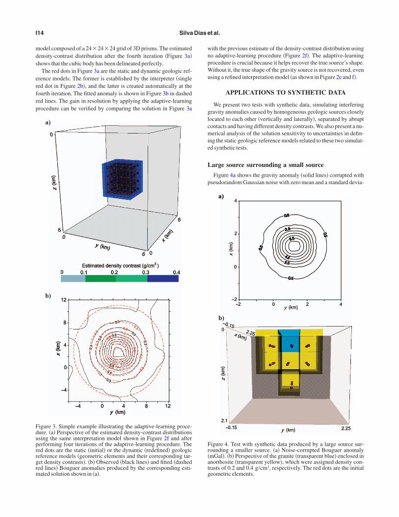
arge source surrounding a small source

Figure 4a shows the gravity anomaly �solid lines� corrupted withseudorandom Gaussian noise with zero mean and a standard devia-

a)a)

b)

igure 4. Test with synthetic data produced by a large source sur-ounding a smaller source. �a� Noise-corrupted Bouguer anomalymGal�. �b� Perspective of the granite �transparent blue� enclosed innorthosite �transparent yellow�, which were assigned density con-rasts of 0.2 and 0.4 g/cm3, respectively. The red dots are the initialeometric elements.

ta0utTtse0pr

a�spgtfi�

tgedryt

tpslsiaa

M

ub2yG0t4std

t7a�

a

b

c

d

FrtiBds


ion of 0.05 mGal. The data at the earth’s surface were computed on13�13 grid in the x- and y-directions, with a grid spacing of

.5 km along both directions. This anomaly was produced by a sim-lated granitic-anorthositic outcropping lopolith �Figure 4b� withhe anorthositic rocks �yellow� surrounding the granitic rocks �blue�.he granite and the anorthosite have positive density contrasts rela-

ive to the metasedimentary country rocks �0.2 and 0.4 g/cm3, re-pectively�. The red dots in Figure 4b define the static geologic refer-nce model whose assigned target density contrasts are 0.2 and.4 g/cm3, depending on whether the interpreter presumes that theoint lies inside the granite �blue� or inside the anorthosite �yellow�,espectively.

Figure 5a-d shows the inversion results after the first to fourth iter-tions, respectively, using � 0.02. The corresponding observedblack lines� and fitted �dashed red lines� gravity anomalies arehown in Figure 5e-h. At the first iteration of the adaptive-learningrocedure, � � 1, the interpretation model consists of a 4�3�3rid of 3D prisms. Figure 5a shows that the estimated density-con-rast distribution does not recover the true lopolith body and does nott the observations �Figure 5e�. At the second �� 2� and third ��

3� iterations of the adaptive-learning procedure, the interpreta-ion models consist of, respectively, an 8�6�6 and a 16�12�12rid of 3D prisms. Figure 5b and c shows the corresponding estimat-d density-contrast distributions, delineating a small source embed-ed in a large source having density contrasts of 0.2 and 0.4 g/cm3,espectively.Additionally, the solutions displayed in Figure 5b and cield acceptable anomaly fits, as shown in Figure 5f and g, respec-ively.

At the fourth iteration of the adaptive-learning procedure, � � 4,he interpretation model consists of a 32�24�24 grid of 3Drisms. The estimated density-contrast distribution and the corre-ponding fitted gravity data are shown in Figure 5d and h, respective-y. The solution at the fourth iteration of the adaptive-learningcheme shows the excellent performance of our method in recover-ng the true granitic-anorthositic lopolith shape. From the fourth iter-tion on, the volumes and geometries of the estimated granite andnorthosite bodies do not vary appreciably.

ultiple buried sources at different depths

Figure 6a displays a perspective view of three buried sources in aniform background producing the ground gravity anomaly, showny black lines in Figure 6b. The data were generated at the nodes of a2�17 grid with sampling intervals of 1 km in both x- and-directions. We corrupt the theoretical anomaly with zero-meanaussian pseudorandom noise with a standard deviation of.01 mGal. The density contrast and the depth to the center of therue sources are 0.15 g/cm3 and 1.5 km �blue block�, 0.3 g/cm3 and

km �green block�, and 0.4 g/cm3 and 2.5 km �red block�. Figure 6chows the set of geometric elements �yellow lines� that representshe static geologic reference model. We assign to these lines targetensity contrasts equal to the corresponding true values.

We invert this gravity anomaly using three iterations of the adap-ive-learning procedure. In all inversions, we set � 0.02. Figurea and b shows the estimated density-contrast distributions at firstnd third iterations, respectively. The corresponding observedblack lines� and fitted �dashed red lines� gravity anomalies are

) e)

) f)

) g)

) h)

igure 5. Test with synthetic data produced by a large source sur-ounding a smaller source. �a-d� Perspectives of the estimated densi-y-contrast distributions after performing, respectively, one to fourterations of the adaptive-learning procedure. �e-h� Noise-corruptedouguer �black lines� and fitted �dashed red lines� anomalies pro-uced by the corresponding estimated solutions shown in �a-d�, re-pectively.

ssgm

upmt�

dtg

Sa

crn�

ptmtdtpgor

jsetba�

taigi

�

�

icPhMb

Fecc�


hown in Figure 7c and d. At the first iteration of the learningcheme, � � 1, the interpretation model consists of a 7�12�6rid of 3D prisms.Although the inversion result �Figure 7a� approxi-ately recovers the three true sources and fits the observations �Fig-

a)

b)

c)

igure 6. Test with synthetic data produced by multiple buried sourc-s at different depths. �a� Perspective of three blocks with densityontrasts of 0.15 �blue�, 0.3 �green�, and 0.4 g/cm3 �red�. �b� Noise-orrupted Bouguer anomaly �mGal�. �c� Initial geometric elementsyellow lines� and true sources �transparent colored blocks�.

re 7c�, we carried out further iterations of the adaptive-learningrocedure until the successive volumes and geometries of the esti-ated sources do not change significantly. The process stops at the

hird iteration, � � 3. The interpretation model, consisting of a 2848�24 grid of 3D prisms, leads to the estimated density-contrast

istribution shown in Figure 7b, which reconstructs very well therue sources and yields a computed anomaly �Figure 7d� that fits theravity data within the experimental errors.

olution sensitivity to uncertainties inpriori information

In this section, we investigate the effect on the previous solutionsaused by small or large perturbations in defining the static geologiceference model. To this end, we repeat the previous two tests using aew set of initial geometric elements as shown in Figure 8a and ddots�, respectively.

In the first test, the new initial geometric elements consist of fouroints only �red dots, Figure 8a�. The purpose is to assess the solu-ion sensitivity to a substantial reduction in the number of initial geo-

etric elements and a slight displacement of its spatial positions. Tohis end, we compare the new results with the previous one �21 redots, Figure 4b�. At the fourth iteration, the estimated density-con-rast distribution �Figure 8b�, obtained with a 48�48�24 3Drisms grid, shows that despite the uncertainties in defining the staticeologic reference model, the estimate still retains the main featuresf the true sources and explains the data within the experimental er-or �Figure 8c�.

In the second test, the new initial geometric elements consist ofust a few points �black dots, Figure 8d�. The purpose is to assess theolution sensitivity to the use of a different type of initial geometriclements �points instead of axes� or to a reduction in the number ofhese elements. We found that the estimated density-contrast distri-ution �Figure 8e� does not reconstruct the true sources very wellnd does not explain the gravity data within the experimental errorsFigure 8f�. In a real example, the interpreter does not know whetherhe estimated and the real sources are close to each other, but he canssess the data misfit and the geologic significance of solution. If hes dissatisfied, he may then reject the solution and try other initialeometric elements until the algorithm produces a solution that sat-sfies the geology and fits the data.

APPLICATION TO REAL DATA

The outcroping Cana Brava layered mafic-ultramafic complexCBC� and the Palmeirópolis volcano-sedimentary sequencePVSS� are located in the north of Goiás state within Tocantins Prov-nce in central Brazil, between the Amazonian and São Franciscoratons. Figure 9 shows a simplified geologic map of the CBC andVSS and adjacent regions �Carminatti et al., 2003�, where the mainost rock consists of metasedimentary sequences of the Serra daesa Group. Figure 10a shows the Bouguer anomaly map produced

y the CBC and PVSS bodies �indicated in Figure 10a�.

re�c�adud�a

vtt

nddePnam

a

b


Because the mafic-ultramafic complex and a volcano-sedimenta-y sequence are outcropping bodies, we define as starting geometriclements at the first iteration �� 1�, a set of points at the surfacecolor dots, Figure 10a�. The blue and red dots have target densityontrasts equal to 0.27 and 0.39 g/cm3, respectively. To all pink dotsFigure 10a� located outside PVSS or CBC outcropping sources, wessign null target density contrasts. We invert this ground gravityata performing two iterations of the adaptive-learning proceduresing � 0.05. At the first iteration of the adaptive-learning proce-ure, � � 1, we set an initial interpretation model consisting of a 3256�5 grid of 3D prisms. Figure 10b shows the fitted Bouguer

nomaly �dashed red lines�, and Figure 11a displays a perspective

)

)

c)

d)

iew of the estimated density-contrast distribution obtained at thehird iteration of the adaptive-learning procedure using an interpre-ation model consisting of a 128�224�20 grid of 3D prisms.

Our result confirms that PVSS and CBC bodies are thin and haveorth-south elongated forms. Jointly, these bodies have horizontalimensions around 86 and 28 km in the north-south and east-westirections, respectively. In Figure 11b, a set of horizontal depth slic-s of the estimated density-contrast distribution shows that theVSS and CBC bodies, between 0 and 4 km, are compact and haveearly constant thicknesses. For depths beyond 4 km, both bodiesre still compact but show variable thicknesses, and they attain aaximum bottom depth of 7 km.

Figure 7. Test with synthetic data produced by mul-tiple buried sources at different depths. �a, b� Per-spective views of the estimated density-contrastdistributions after performing, respectively, oneand three iterations of the adaptive-learning proce-dure. �c, d� Noise-corrupted Bouguer �black lines�and fitted �dashed red lines� anomalies produced bythe corresponding inversion solutions shown in �a�and �b�, respectively.

Favd4a�fic�


a) d)

b) e)

c)

f)

igure 8. Solution sensitivity to uncertainties in thepriori information. �a, b� and �d, e� Perspective

iews of the true and the estimated density-contrastistributions of the synthetic tests shown in Figuresand 6, respectively. The �a� red and �d� black dotsre the corresponding initial geometric elements.c, f� Noise-corrupted Bouguer �black lines� andtted �dashed red lines� anomalies produced by theorresponding inversion solutions shown in �b� ande�, respectively.

a


Figure 9. Simplified geologic map of Cana Brava layered mafic-ul-tramafic complex �CBC� and the Palmeirópolis volcano-sedimenta-ry sequence �PVSS� in central Brazil.After Carminatti et al. �2003�.

) b) Figure 10. �a� Bouguer anomaly map �gray lines�from the Cana Brava layered mafic-ultramaficcomplex �CBC� and the Palmeirópolis volcano-sedimentary sequence �PVSS� and adjacent re-gions in central Brazil. The blue, red, and pink dotsare the first guesses of the geometric elements withtarget density contrasts equal to 0.27, 0.39, and0.0 g/cm3, respectively. The black line indicatesthe outcropping boundary separating the CBC andPVSS from the host rock. �b� Observed �solid blacklines� and fitted �dashed red lines� Bouguer anoma-lies obtained at the second iteration of the adaptive-learning procedure.

mstplr

Te

istpdea

Teosattt

Aeiaf�S51P

B

—

B

B

B

B

C

C

C

G

K

L

L

P

a

b

Fdah


CONCLUSIONS

We have proposed an iterative and interactive gravity inversionethod to estimate a 3D density-contrast distribution; it fits the ob-

ervations within the measurement errors and favors compact gravi-y sources closest to the skeletal outlines of the sources. The inter-reter guides the inversion by specifying the first-guess skeletal out-ines as well as their associated density contrasts and by accepting orejecting the solution.

This method has been tested on both synthetic and field data sets.he results show that the method is effective in retrieving the geom-tries of multiple gravity sources that give rise to an interfering grav-

)

)

igure 11. Cana Brava layered mafic-ultramafic complex. Estimatedensity-contrast distribution obtained at the third iteration of thedaptive-learning procedure. �a� Perspective view. �b� Ensemble oforizontal depth slices

ty anomaly without introducing depth weighting or integrated sen-itivities of the data vector to each parameter to avoid concentratinghe estimated mass at the surface. The method significantly helps im-rove image sharpness. Therefore, it can be used to interpret gravityata from a geologic setting consisting of sharp-boundary domains,.g., intrusive rocks in sedimentary environments such as laccolithsnd sills, regardless of whether their shapes are simple or complex.

Our method can be used in two different interpretation contexts.he first is the case where the required a priori information may beasily retrieved from available geological data. The user may acceptr reject a solution on the basis of his geologic conception about theources and, in either case, start a new inversion modifying the initialpriori information. The method is therefore a tool in helping, rather

han replacing, geophysicists in decision-making. In the second con-ext, the a priori information cannot be retrieved easily. In this case,he method can be used to test a variety of geological hypotheses.

ACKNOWLEDGMENTS

The authors thank editor Kees Wapenaar, assistant editor Stevenrcone, associate editor John Peirce, and three anonymous review-

rs for helpful comments. We thank Yara R. Marangoni for provid-ng the real gravity data and for helpful discussions. V. C. F. Barbosand J. B. C. Silva were supported in this research by fellowshipsrom Conselho Nacional de Desenvolvimento e TecnológicoCNPq�, Brazil. Additional support for V. C. F. Barbosa and F. J. S.ilva Dias was provided by CNPq �grants 471913/2007-3 and01749/2008-0� and FAPERJ �grants E-26/100.688/2007 and E-26/10.961/2008�. Most of the figures were done with the open-sourcearaView program.

REFERENCES

arbosa, V. C. F., and J. B. C. Silva, 1994, Generalized compact gravity in-version: Geophysics, 59, 57–68.—–, 2006, Interactive 2D magnetic inversion: A tool for aiding forwardmodeling and testing geologic hypotheses: Geophysics, 71, no. 5, L43–L50.

arbosa, V. C. F., J. B. C. Silva, and W. E. Medeiros, 2002, Practical applica-tions of uniqueness theorems in gravimetry: Part II — Pragmatic incorpo-ration of concrete geologic information: Geophysics, 67, 795–800.

ertete-Aguirre, H., E. Cherkaev, and M. Oristaglio, 2002, Non-smoothgravity problem with total variation penalization functional: GeophysicalJournal International, 149, 499–507.

lakely, R. J., 1995, Potential theory in gravity and magnetic applications:Cambridge University Press.

osch, M., R. Meza, R. Jiménez, and A. Hönig, 2006, Joint gravity and mag-netic inversion in 3D using Monte Carlo methods: Geophysics, 71, no. 4,G153–G156.

amacho, A. G., F. G. Montesinos, and R. Vieira, 2000, Gravity inversion bymeans of growing bodies: Geophysics, 65, 95–101.

arminatti, M. G., Y. R. Marangoni, and C. T. Correia, 2003, Modelagemgravimétrica do complexo de Cana Brava e seqüência de Palmeirópolis,GO: Revista Brasileira de Geociências, 33, 245–254.

hen, S., and Z. Gao, 2007, A new method of gravity inversion based on thefrequency characteristic of density distribution: 77th Annual InternationalMeeting, SEG, ExpandedAbstracts, 811–815.

uillen, A., and V. Menichetti, 1984, Gravity and magnetic inversion withminimization of a specific functional: Geophysics, 49, 1354–1360.

irkendall, B., Y. Li, and D. Oldenburg, 2007, Imaging cargo containers us-ing gravity gradiometry: IEEE Transactions in Geoscience and RemoteSensing, 45, 1786–1797.

ast, B. J., and K. Kubik, 1983, Compact gravity inversion: Geophysics, 48,713–721.

i, Y., and D. W. Oldenburg, 1998, 3-D inversion of gravity data: Geophys-ics, 63, 109–119.

ortniaguine, O., and M. S. Zhdanov, 1999, Focusing geophysical inversionimages: Geophysics, 64, 874–887.

R

R

S

S

—

S

S

T

Y

Z

Z


amos, F. M., H. F. Campos Velho, J. C. Carvalho, and N. J. Ferreira, 1999,Novel approaches on entropic regularization: Inverse Problems, 15, 1139–1148.

oy, A., 1962, Ambiguity in geophysical interpretation: Geophysics, 27, 90–99.

ilva, J. B. C., and V. C. F. Barbosa, 2006, Interactive gravity inversion: Geo-physics, 71, no. 1, J1–J9.

ilva, J. B. C., W. E. Medeiros, and V. C. F. Barbosa, 2001, Potential field in-version: Choosing the appropriate technique to solve a geologic problem:Geophysics, 66, 511–520.—–, 2002, Practical applications of uniqueness theorems in gravimetry:Part I — Constructing sound interpretation methods: Geophysics, 67,788–794.

ilva, J. B. C., F. S. Oliveira, V. C. F. Barbosa, and H. F. Campos Velho, 2007,Apparent-density mapping using entropic regularization: Geophysics, 72,no. 4, I51–I60.

tark, P. B., 1997, Does God play dice with the earth? �And if so, are theyloaded?�: Presented at the SIAM Geosciences Meeting, unpublished notesavailable at http://www.stat.berkeley.edu/users/stark/accessed 6 February2009.

ikhonov, A. N., and V. Y. Arsenin, 1977, Solutions of ill-posed problems: V.H. Winston & Sons.

ao, C., 2007, Iterative 3-D gravity and magnetic inversion for physicalproperties: 77thAnnual International Meeting, SEG, ExpandedAbstracts,805–809.

hang, J., C. Wang, Y. Shiz, Y. Cai, W. Chi, D. Dreger, W. Cheng, and Y.Yuan, 2004, Three-dimensional crustal structure in central Taiwan fromgravity inversion with a parallel genetic algorithm: Geophysics, 69,917–924.

hdanov, M. S., R. Ellis, and S. Mukherjee, 2004, Three-dimensional regu-larized focusing inversion of gravity gradient tensor component data:Geophysics, 69, 925–937.

3D gravity inversion through an adaptive-learning procedure

Documents

Transcript of 3D gravity inversion through an adaptive-learning procedure