A NEW PROCEDURE TO PERFORM DIFFERENTIAL UNDERGROUND GRAVITYMEASUREMENTS.

G.RANIERIDipartimento di Georisorse e Territorio - Politecnico di Torino - Italy.

L.SAMBUELLIDipartimento di Ingegneria del Territorio - Università di Cagliari - Italy.

Abstract

The aim of this research is to evaluate the possibility of using underground gravity measurements in order tocharacterise density anomalies in tunnel surroundings. A measurement procedure which allows estimation ofthe gravimetrical differential effects in several directions is proposed. Attention is paid to the theoreticalaspects and a method is then put forward for carrying out a practical survey.

Foreword

The characterisation of voids or of altered or mineralised rock volumes in road, railway or mining tunnelsurroundings is of great importance in geotechnical engineering and mining research.

Gravity measurement methods can be used, together with other geophysical methods, for such a purpose.

As the characterisation of anomalous bodies can be difficult when the survey is carried out from thesurface, the possibilities offered by underground measurements, i.e. measurements closer to the source ofthe anomaly, are examined.

Various authors (Smith, 1950), (Hammer,1950), (Domzalski,1955), (Hussein et al.,1981), (Murty etal.,1982), (Fajklewicz,1983), (Casten et al.,1989) and (Nekut,1989) have studied the problemsconnected with underground gravimetric measurements. Others have pointed out the potentiality of themeasurement of gravitational gradients (Fajklewicz,1976), (Butler,1984) and (Klingelé,1991), and stillothers (Arzi,1975) have presented the results of gravimetric and microgravimetric prospecting carried outfor engineering purposes.

The measurement of vertical gravity gradients underground is particularly suited to proving the existence ofanomalous bodies, but it does not allow the exact positioning of the source around a tunnel. The theoreticalaspects and the true applicability of a procedure which is capable of giving, with a high degree of reliability,the position of an anomalous body around a tunnel will be examined here.

Operating procedure

The proposed procedure fundamentally implies:

1) carrying out N measurement l i , at constant angular intervals, with a return to the starting point, along themaximum circumference inscribed in the tunnel section and orthogonal to its axis;

2) carrying out the said measurements li j, in several equally spaced sections along the axis of the tunnel and

perpendicular to it;3) the subtraction , in the same tunnel section, of values obtained from the gravimeter in positions which are

symmetric with respect to the tunnel axis and defined as “conjugate” positions, viz. :

( )c l li i N i= −+ 2

and a further subtraction of the values so obtained in adjoining or homologous sections:

( )g c i j ci j i j, ,,= −+1

.

In this way, two sets of differential effects are calculated: one set along various diameters of the section, theother along the tunnel axis.

The outstanding aspects of this procedure are:

a) a vectorization of gravimetric indications (given essentially by the diametrical differences) which, togetherwith the study of the values read in the single positions, allows one to obtain the zenithal angle of theanomalous body in a section,

b) the attenuation of the anomalies at large wavelength (given, not only but essentially, by the gradient alongthe axis) which allows one to localise the anomalous body along the direction of the tunnel.

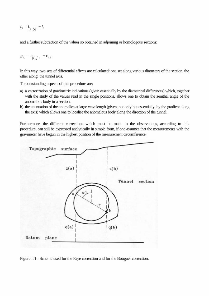
Furthermore, the different corrections which must be made to the observations, according to thisprocedure, can still be expressed analytically in simple form, if one assumes that the measurements with thegravimeter have begun in the highest position of the measurement circumference.

Figure n.1 - Scheme used for the Faye correction and for the Bouguer correction.

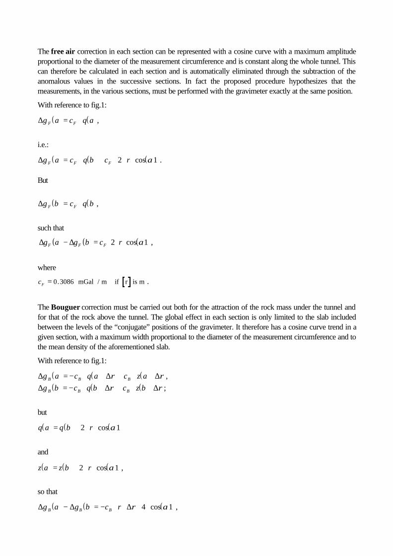
The free air correction in each section can be represented with a cosine curve with a maximum amplitudeproportional to the diameter of the measurement circumference and is constant along the whole tunnel. Thiscan therefore be calculated in each section and is automatically eliminated through the subtraction of theanomalous values in the successive sections. In fact the proposed procedure hypothesizes that themeasurements, in the various sections, must be performed with the gravimeter exactly at the same position.

With reference to fig.1:

( ) ( )∆g a c q aF F= ⋅ ,

i.e.:

( ) ( ) ( )∆g a c q b c rF F F= ⋅ + ⋅ ⋅ ⋅2 1cos α .

But

( ) ( )∆g b c q bF F= ⋅ ,

such that

( ) ( ) ( )∆ ∆g a g b c rF F F− = ⋅ ⋅ ⋅2 1cos α ,

where

cF = 0 3086. mGal / m if r is m .

The Bouguer correction must be carried out both for the attraction of the rock mass under the tunnel andfor that of the rock above the tunnel. The global effect in each section is only limited to the slab includedbetween the levels of the “conjugate” positions of the gravimeter. It therefore has a cosine curve trend in agiven section, with a maximum width proportional to the diameter of the measurement circumference and tothe mean density of the aforementioned slab.

With reference to fig.1:

( ) ( ) ( )∆ ∆ ∆g a c q a c z aB B B= − ⋅ ⋅ + ⋅ ⋅ρ ρ,( ) ( ) ( )∆ ∆ ∆g b c q b c z bB B B= − ⋅ ⋅ + ⋅ ⋅ρ ρ;

but

( ) ( ) ( )q a q b r= + ⋅ ⋅2 1cos α

and

( ) ( ) ( )z a z b r= + ⋅ ⋅2 1cos α ,

so that

( ) ( ) ( )∆ ∆ ∆g a g b c rB B B− = − ⋅ ⋅ ⋅ ⋅ρ α4 1cos ,

with

[ ] [ ]cB = 0 04192. mGal / m if is g / cm and r is m3∆ρ .

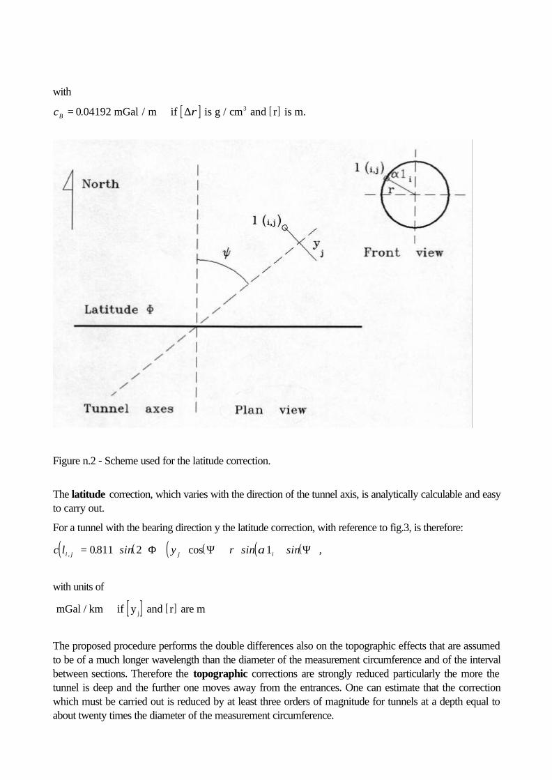
Figure n.2 - Scheme used for the latitude correction.

The latitude correction, which varies with the direction of the tunnel axis, is analytically calculable and easyto carry out.

For a tunnel with the bearing direction y the latitude correction, with reference to fig.3, is therefore:

( ) ( ) ( ) ( ) ( )( )c l sin y r sin sini j j i, . cos= ⋅ ⋅ ⋅ ⋅ + ⋅ ⋅0811 2 1Φ Ψ Ψα ,

with units of

[ ] [ ] mGal / km if y and r are mj

The proposed procedure performs the double differences also on the topographic effects that are assumedto be of a much longer wavelength than the diameter of the measurement circumference and of the intervalbetween sections. Therefore the topographic corrections are strongly reduced particularly the more thetunnel is deep and the further one moves away from the entrances. One can estimate that the correctionwhich must be carried out is reduced by at least three orders of magnitude for tunnels at a depth equal toabout twenty times the diameter of the measurement circumference.

A further correction which should be mentioned is that caused by the presence of the tunnel itself.However, if the tunnel section is constant and the measurements are carried out on the maximum inscribedcircumference, it is automatically eliminated when one takes the gradient along the tunnel.

The lunisolar and instrumental drift effects can be subtracted from the measurement by the usualprocedure of systematic parallel readings at a fixed station.

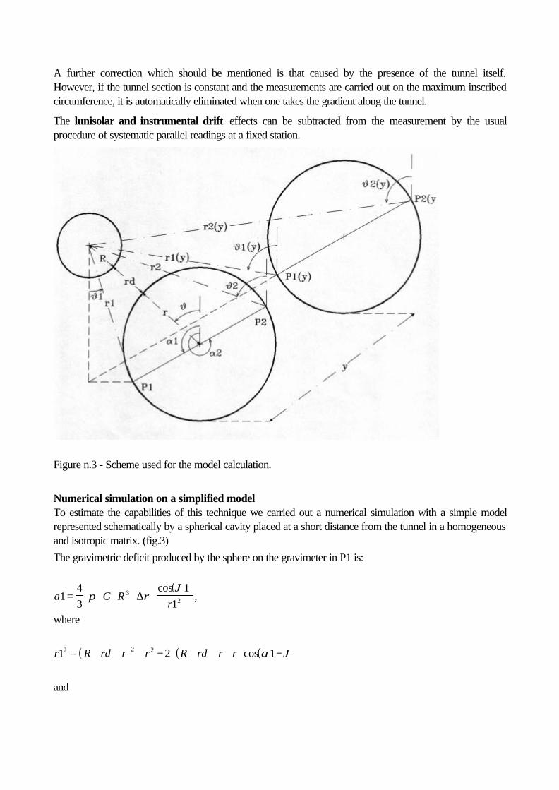
Figure n.3 - Scheme used for the model calculation.

Numerical simulation on a simplified modelTo estimate the capabilities of this technique we carried out a numerical simulation with a simple modelrepresented schematically by a spherical cavity placed at a short distance from the tunnel in a homogeneousand isotropic matrix. (fig.3)

The gravimetric deficit produced by the sphere on the gravimeter in P1 is:

( )a G R

r1

43

11

32= ⋅ ⋅ ⋅ ⋅ ⋅π ρϑ

∆cos

,

where

( ) ( ) ( )r R rd r r R rd r r1 2 12 2 2= + + + − ⋅ + + ⋅ ⋅ −cos α ϑ

and

( )ϑ ϑ α ϑ11

1= − ⋅ −

arcsin

rr

sin .

In order to obtain the effect on the gravimeter in P2 it is sufficient to replace the scanning angle α1 byα2=α1+π in the preceding expression, which yields:

( ) ( ) ( )r R rd r r R rd r r2 2 22 2 2= + + + − ⋅ + + ⋅ ⋅ −cos α ϑ ,

where

( )ϑ ϑ α ϑ22

2= − ⋅ −

arcsin

rr

sin ,

and therefore

( )a G R

r2

43

22

32= ⋅ ⋅ ⋅ ⋅ ⋅π ρ

ϑ∆

cos.

As far as the calculation relative to the homologous positions of P1 and P2 is concerned in a measurementsection y meters distant from that passing through the centre of the anomalous sphere, it is sufficient toconsider that:

( )r y r y1 12 2= + ,

( )r y r y2 22 2= + ,

( ) ( )( )ϑ ϑ1

1

11y

r

r y= ⋅

arccos cos ,

( ) ( ) ( )ϑ ϑ22

22y

r

r y= ⋅

arccos cos ,

and therefore

( ) ( )( )( )a y G R

y

r y1

43

1

13

2= ⋅ ⋅ ⋅ ⋅ ⋅π ρϑ

∆cos

,

( ) ( )( )( )a y G R

y

r y2

43

2

23

2= ⋅ ⋅ ⋅ ⋅ ⋅π ρϑ

∆cos

.

For this model the gravimetric differential effects were calculated both in a section along the tunnel fordifferent radial distances and zenithal angles, and for different dimensions and densities of the anomaloussphere. In order to estimate topographic effects a large diameter sphere was assumed which simulated(fig.4) a topographic lateral effect.The diametrical gravity differences in a tunnel section using a measuring circumference radius of 2m, for a2m radius sphere with a density contrast of 2.5 g/cm3 , centred 6m from the tunnel axes, were calculated.To check the effectiveness of the method, in giving indications on the true zenithal angle of the anomaloussphere centre (θ), simulations were performed with spheres having their centres at a zenithal angle ofrespectively 0°, 30°, 60° and 90°. In fig.5 the diametrical differences, obtained by the aforesaid simulation,are plotted versus the scanning angle α1.

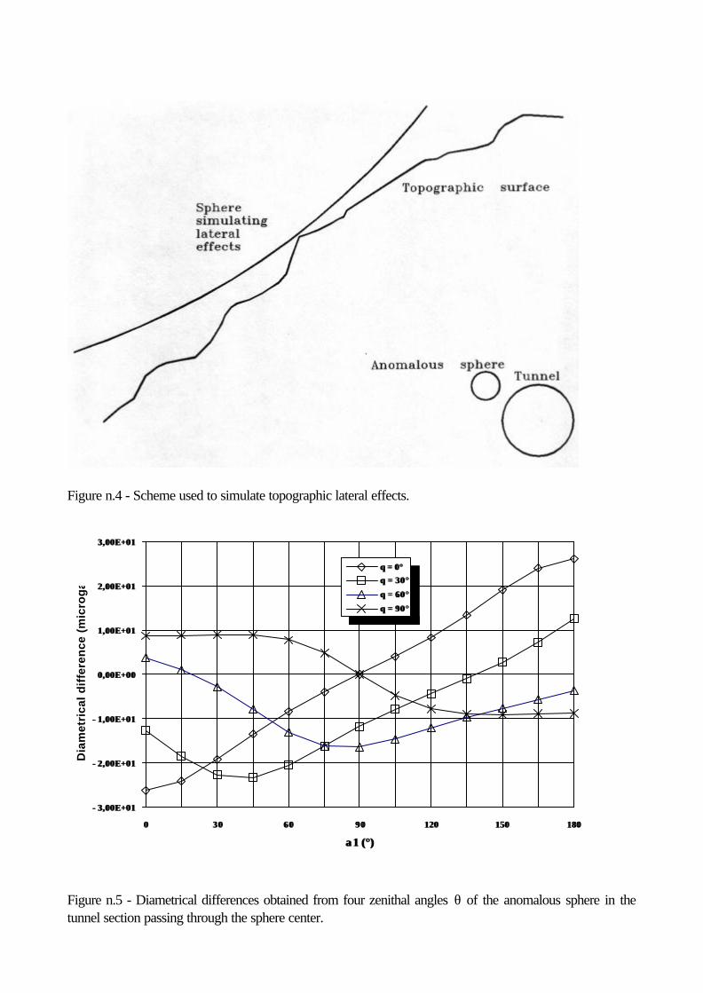
Figure n.4 - Scheme used to simulate topographic lateral effects.

α1 (°)α1 (°)

Dia

met

rica

l d

iffe

ren

ce (

mic

rog

al)

−3,00Ε+01−3,00Ε+01

−2,00Ε+01−2,00Ε+01

−1,00Ε+01−1,00Ε+01

0,00Ε+000,00Ε+00

1,00Ε+011,00Ε+01

2,00Ε+012,00Ε+01

3,00Ε+013,00Ε+01

00 3030 6060 9090 120120 150150 180180

θ = 0°θ = 0°θ = 30°θ = 30°

θ = 60°θ = 60°

θ = 90°θ = 90°

Figure n.5 - Diametrical differences obtained from four zenithal angles θ of the anomalous sphere in thetunnel section passing through the sphere center.

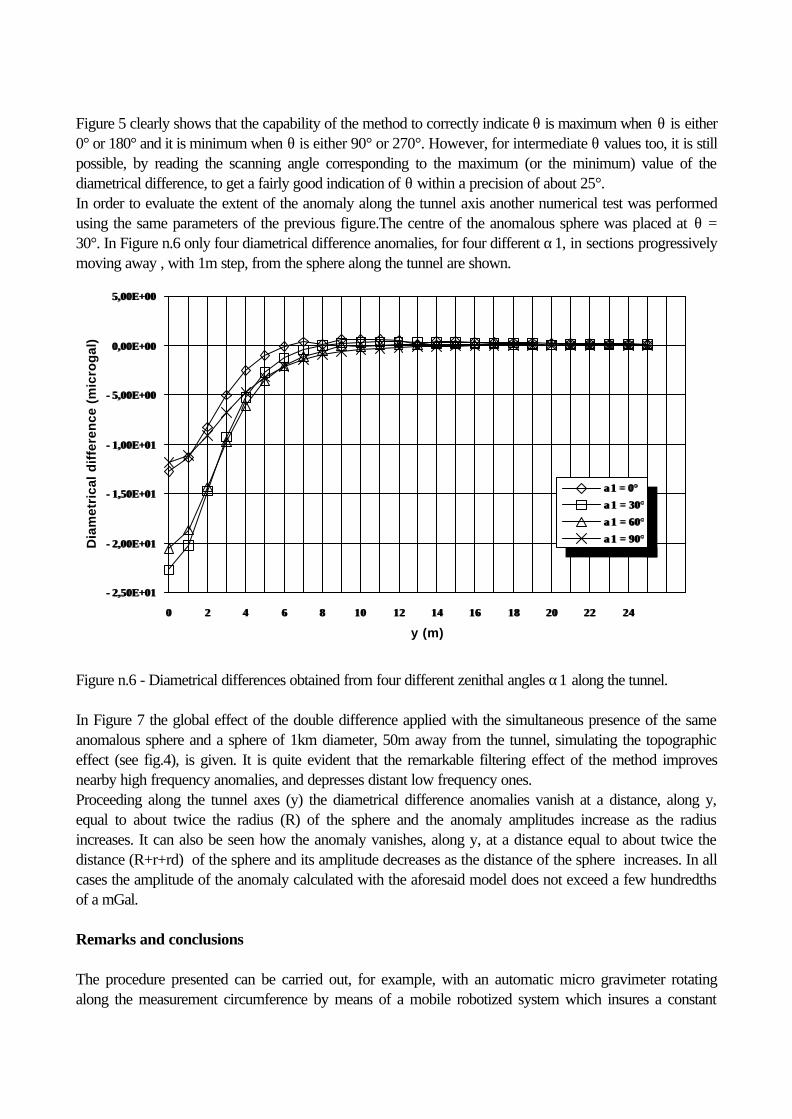
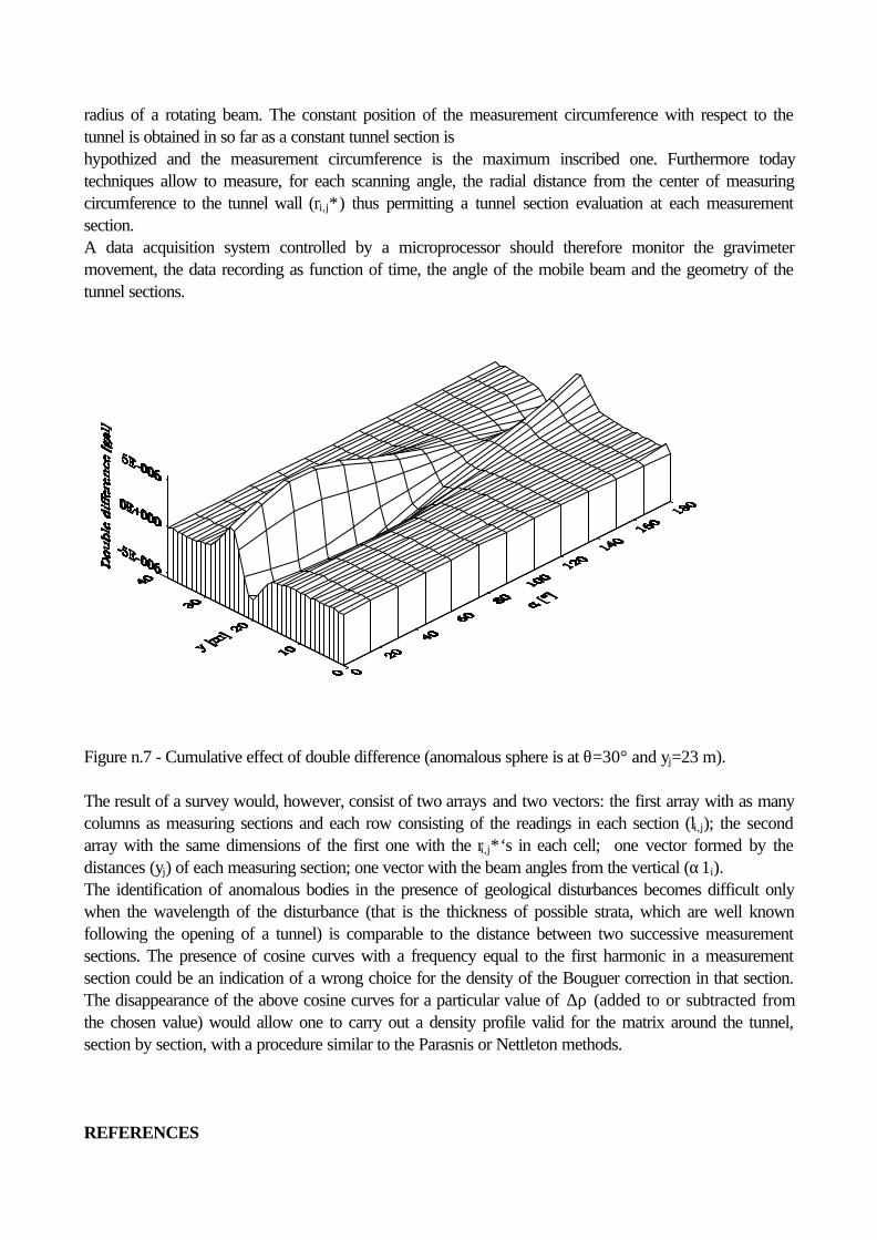
Figure 5 clearly shows that the capability of the method to correctly indicate θ is maximum when θ is either0° or 180° and it is minimum when θ is either 90° or 270°. However, for intermediate θ values too, it is stillpossible, by reading the scanning angle corresponding to the maximum (or the minimum) value of thediametrical difference, to get a fairly good indication of θ within a precision of about 25°.In order to evaluate the extent of the anomaly along the tunnel axis another numerical test was performedusing the same parameters of the previous figure.The centre of the anomalous sphere was placed at θ =30°. In Figure n.6 only four diametrical difference anomalies, for four different α1, in sections progressivelymoving away , with 1m step, from the sphere along the tunnel are shown.

y (m)

Dia

met

rica

l d

iffe

ren

ce (

mic

rog

al)

−2,50Ε+01−2,50Ε+01

−2,00Ε+01−2,00Ε+01

−1,50Ε+01−1,50Ε+01

−1,00Ε+01−1,00Ε+01

−5,00Ε+00−5,00Ε+00

0,00Ε+000,00Ε+00

5,00Ε+005,00Ε+00

00 22 44 66 88 1010 1212 1414 1616 1818 2020 2222 2424

α1 = 0°α1 = 0°

α1 = 30°α1 = 30°

α1 = 60°α1 = 60°

α1 = 90°α1 = 90°

Figure n.6 - Diametrical differences obtained from four different zenithal angles α1 along the tunnel.

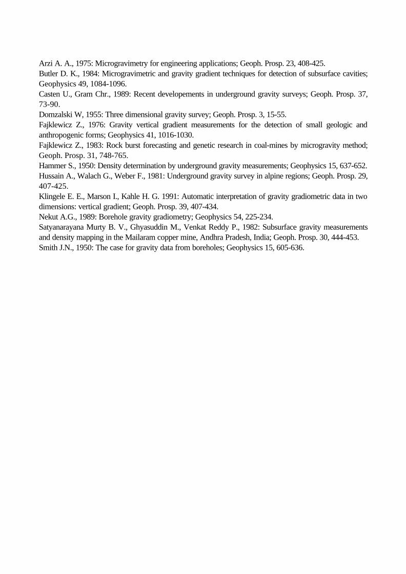
In Figure 7 the global effect of the double difference applied with the simultaneous presence of the sameanomalous sphere and a sphere of 1km diameter, 50m away from the tunnel, simulating the topographiceffect (see fig.4), is given. It is quite evident that the remarkable filtering effect of the method improvesnearby high frequency anomalies, and depresses distant low frequency ones.Proceeding along the tunnel axes (y) the diametrical difference anomalies vanish at a distance, along y,equal to about twice the radius (R) of the sphere and the anomaly amplitudes increase as the radiusincreases. It can also be seen how the anomaly vanishes, along y, at a distance equal to about twice thedistance (R+r+rd) of the sphere and its amplitude decreases as the distance of the sphere increases. In allcases the amplitude of the anomaly calculated with the aforesaid model does not exceed a few hundredthsof a mGal.

Remarks and conclusions

The procedure presented can be carried out, for example, with an automatic micro gravimeter rotatingalong the measurement circumference by means of a mobile robotized system which insures a constant

radius of a rotating beam. The constant position of the measurement circumference with respect to thetunnel is obtained in so far as a constant tunnel section ishypothized and the measurement circumference is the maximum inscribed one. Furthermore todaytechniques allow to measure, for each scanning angle, the radial distance from the center of measuringcircumference to the tunnel wall (ri,j∗) thus permitting a tunnel section evaluation at each measurementsection.A data acquisition system controlled by a microprocessor should therefore monitor the gravimetermovement, the data recording as function of time, the angle of the mobile beam and the geometry of thetunnel sections.

Figure n.7 - Cumulative effect of double difference (anomalous sphere is at θ=30° and yj=23 m).

The result of a survey would, however, consist of two arrays and two vectors: the first array with as manycolumns as measuring sections and each row consisting of the readings in each section (li,j); the secondarray with the same dimensions of the first one with the ri,j∗‘s in each cell; one vector formed by thedistances (yj) of each measuring section; one vector with the beam angles from the vertical (α1i).The identification of anomalous bodies in the presence of geological disturbances becomes difficult onlywhen the wavelength of the disturbance (that is the thickness of possible strata, which are well knownfollowing the opening of a tunnel) is comparable to the distance between two successive measurementsections. The presence of cosine curves with a frequency equal to the first harmonic in a measurementsection could be an indication of a wrong choice for the density of the Bouguer correction in that section.The disappearance of the above cosine curves for a particular value of ∆ρ (added to or subtracted fromthe chosen value) would allow one to carry out a density profile valid for the matrix around the tunnel,section by section, with a procedure similar to the Parasnis or Nettleton methods.

REFERENCES

Arzi A. A., 1975: Microgravimetry for engineering applications; Geoph. Prosp. 23, 408-425.Butler D. K., 1984: Microgravimetric and gravity gradient techniques for detection of subsurface cavities;Geophysics 49, 1084-1096.Casten U., Gram Chr., 1989: Recent developements in underground gravity surveys; Geoph. Prosp. 37,73-90.Domzalski W, 1955: Three dimensional gravity survey; Geoph. Prosp. 3, 15-55.Fajklewicz Z., 1976: Gravity vertical gradient measurements for the detection of small geologic andanthropogenic forms; Geophysics 41, 1016-1030.Fajklewicz Z., 1983: Rock burst forecasting and genetic research in coal-mines by microgravity method;Geoph. Prosp. 31, 748-765.Hammer S., 1950: Density determination by underground gravity measurements; Geophysics 15, 637-652.Hussain A., Walach G., Weber F., 1981: Underground gravity survey in alpine regions; Geoph. Prosp. 29,407-425.Klingele E. E., Marson I., Kahle H. G. 1991: Automatic interpretation of gravity gradiometric data in twodimensions: vertical gradient; Geoph. Prosp. 39, 407-434.Nekut A.G., 1989: Borehole gravity gradiometry; Geophysics 54, 225-234.Satyanarayana Murty B. V., Ghyasuddin M., Venkat Reddy P., 1982: Subsurface gravity measurementsand density mapping in the Mailaram copper mine, Andhra Pradesh, India; Geoph. Prosp. 30, 444-453.Smith J.N., 1950: The case for gravity data from boreholes; Geophysics 15, 605-636.