Reverse Engineering of Gene Regulatory Network by Integration of Prior Global Gene Regulatory...

Genome Biology 2003, 4:P5

Deposited research articleReverse engineering of gene regulatory networks: a finite statelinear modelAlvis Brazma and Thomas Schlitt

Addresses: EMBL European Bioinformatics Institute, Wellcome Trust Genome Campus, Hinxton, Cambridge CB10 1SD, UK.

Correspondence: Thomas Schlitt. E-mail: [email protected]

com

ment

reviews

reports

deposited research

interactions

inform

ation

refereed research

.deposited research

AS A SERVICE TO THE RESEARCH COMMUNITY, GENOME BIOLOGY PROVIDES A 'PREPRINT' DEPOSITORY

TO WHICH ANY ORIGINAL RESEARCH CAN BE SUBMITTED AND WHICH ALL INDIVIDUALS CAN ACCESS

FREE OF CHARGE. ANY ARTICLE CAN BE SUBMITTED BY AUTHORS, WHO HAVE SOLE RESPONSIBILITY FOR

THE ARTICLE'S CONTENT. THE ONLY SCREENING IS TO ENSURE RELEVANCE OF THE PREPRINT TO

GENOME BIOLOGY'S SCOPE AND TO AVOID ABUSIVE, LIBELLOUS OR INDECENT ARTICLES. ARTICLES IN THIS SECTION OF

THE JOURNAL HAVE NOT BEEN PEER-REVIEWED. EACH PREPRINT HAS A PERMANENT URL, BY WHICH IT CAN BE CITED.

RESEARCH SUBMITTED TO THE PREPRINT DEPOSITORY MAY BE SIMULTANEOUSLY OR SUBSEQUENTLY SUBMITTED TO

GENOME BIOLOGY OR ANY OTHER PUBLICATION FOR PEER REVIEW; THE ONLY REQUIREMENT IS AN EXPLICIT CITATION

OF, AND LINK TO, THE PREPRINT IN ANY VERSION OF THE ARTICLE THAT IS EVENTUALLY PUBLISHED. IF POSSIBLE, GENOME

BIOLOGY WILL PROVIDE A RECIPROCAL LINK FROM THE PREPRINT TO THE PUBLISHED ARTICLE.

Posted: 29 April 2003


The electronic version of this article is the complete one and can befound online at http://genomebiology.com/2003/4/6/P5

© 2003 BioMed Central Ltd

Received: 14 April 2003

This is the first version of this article to be made available publicly.

This information has not been peer-reviewed. Responsibility for the findings rests solely with the author(s).

2 Genome Biology Deposited research (preprint)


Reverse Engineering of Gene Regulatory Networks:

a Finite State Linear Model

Alvis Brazma and Thomas Schlitt

European Bioinformatics Institute1

1 EMBL-EBI, Wellcome Trust Genome Campus, Hinxton, Cambridge CB10 1SD, United Kingdom,

[email protected], tel. +44-1223-494651, fax +44-1223-494468

http://genomebiology.com/2003/4/6/P5 Genome Biology 2003, Volume 4, Issue 6, Article P5 Brazma and Schlitt. P5.3


Abstract

We propose a new model for describing gene regulatory networks that can capture discrete

(Boolean) and continuous (differential) aspects of gene regulation. After giving some

illustrations of the model, we study the problem of the reverse engineering of such networks,

i.e., how to construct a network from gene expression data. We prove that for our model there

exists an algorithm finding a network compatible with the given data. We demonstrate the

model by simulating lambda-phage. We also describe some generalizations of the model,

discuss their relevance to the real-world gene networks and formulate a number of open

problems.

Keywords: gene regulation, regulatory networks, regulatory circuits, dynamic systems, finite

state automata, reverse engineering

Background

There are many mechanisms how genes are regulated. An important role in gene regulation

apparently is played by specific proteins, called transcription factors, which influence the

transcription of particular genes by binding to specific parts of the DNA in the genome. In

this way a product of one gene can influence the expression of another gene, and we can

consider a network of gene regulation. Such regulatory networks or circuits are well studied

in lambda-phage and some other viruses[1]. If the network involves only few genes, its

functioning can be understood relatively directly. But what does it mean to understand a gene

regulatory network of hundreds or thousands of genes? Just describing such a network may be

highly nontrivial. We think that to be able to understand complex gene regulatory networks,

first a formal language for describing such networks has to be developed. The language can



be graph based and preferably should allow the simulation of the behaviour of the network.

By simulating a network we can make predictions and compare them to experimental data. If

the predictions are consistent with the data, then we can say that the model is correct (within

the given accuracy limits). Such an approach is usual in physics: models (theories) are built to

explain existing data, then predictions are made, which again are compared to new data. If the

correspondence is good, it is claimed that the phenomenon has been understood. Preferably,

the model should not be a black box, but should be interpretable, and ideally its elements

should have interpretation in the real world consistent with the existing knowledge. At the

same time, each model involves a simplification of the real world, which is a part of the

strength of the modelling approaches.

Various models for gene regulatory networks have been proposed and studied (see for

instance [2, 3]). In general these models fall into two categories: boolean network based

models, for instance [4-6], and dynamic systems described by differential or difference

equations, for instance [7, 8]. Each of these models have their advantages and drawbacks. The

Boolean model is based on the assumption that the important aspects of gene regulation can

be described by binary on/off switches, functioning in discrete time steps: the state of the

network in time point n is determined by its state at time-point n-1. Even if we generalize

these models to more than two discrete states they cannot describe continuous changes that

happen in the cell environment. These can be described by differential equation based models,

which on the other hand cannot easily describe the discrete aspects of gene regulation such as

binding of a transcription factor to the DNA, which is essentially an on/off event. Also, in a

differential equation model it is difficult (though not impossible) to describe non-additive

logics in gene regulation (for instance, competitive events), as well as time delays.



Models trying to combine the discrete and continuous components have been proposed, for

instance in [9-11]. Thomas and Thieffry [12, 13] describe a combined model for qualitative

description of gene regulatory networks. They introduce a notion of gene state and image, the

last effectively representing the substance produced by the respective gene. There is a time

delay between the change of the gene state and the change of the image state. By introducing

different levels of gene activity and thresholds for switching the gene states, thus they go

beyond binary models. They study the qualitative behaviours of various feed-back loops in

their model, and show that they fall into two classes: positive loops leading to multi stable

states and negative ones leading to periodicity.

The finite state linear model proposed in this paper combines the discrete and continuous

aspects of gene regulation in a simple and structured way. It has a boolean network type

discrete control component, and an environment of substances changing their concentrations

continuously. Time is continuous, and the state of the network directly determines only the

concentration change rates, while the state is affected by the concentrations themselves.

A framework (a formal language) for describing gene regulatory networks enables us to study

the problem of building particular models from gene expression data -often referred to as the

reverse engineering of gene networks (e.g., [3, 5]). Until recently there were little quantitative

data available for building models for gene regulation. Most of the earlier gene network

models, including [13] are based on observations from gene mutation data leading to

phenomenological changes and not on direct observations of gene activities. This has changed

with the advent of DNA microarray technology, which generates huge amounts of data

characterizing gene activities under various conditions [14-16] and are now being collected in

various databases [17]. There can be various precise formulations for the reverse engineering



problem, and there is a certain analogy between the problems of reverse engineering of gene

networks and the problem of identifying finite state automata from input/output data [18].

In this paper we consider two different formulations of the reverse engineering problem. The

weakest one is finding a gene network consistent with the given data. We prove that this

problem is algorithmically solvable for our model. The second one involves assuming that the

data have been produced by some unknown gene network, which we want to reconstruct by

making experiments. This problem is still open. In the next section we describe the model,

after which we study the reverse engineering problem. Then we give some informal extension

of the model, and use it to describe the lambda-phage regulatory circuit. Finally we discuss

some open problems.

Results and Discussion

The definition of the model

The assumptions on which our model is based are: (1) the gene activity is determined by the

state of transcription factor binding sites in its promoter region; (2) each binding site can be in

one of a finite number of states, characterized by having or not having bound a particular

transcription factor; (3) depending on the states of the binding sites in the promoter, the gene

can either be silent, or have a particular activity level; (4) if a gene is active, the concentration

of the substance it produces is growing with a rate dependent on the activity level of the gene,

otherwise it is decreasing (or staying 0); (5) the state of a binding site depends on the

concentration of the respective transcription factor(s). To make these assumptions precise and

to formalize them we have developed the model described below. We begin by describing a

simpler version of the model, which we call the binary model, where each binding site and



each gene have only two states: on or off. We formulate the reverse engineering problem for

the binary model, before introducing the general case, though the formulation remains the

same in the general case.

The binary model

Informally we assume that we have an environment of n substances 1, … , n having

concentrations c1(t), … , cn(t), respectively, which may change in time t. We also assume that

there are, what we call substance binding sites in the environment, each of which can attach

(bind) a specific substance. In the binary case the binding site can bind only one substance.

We define a binary binding site b as a triple

b=(i, a, d),

where i is the number of the substance (which can bind to b), and a and d are positive real

constants 0<d<a, called association and dissociation constants, respectively. Each binding

site can be in one of two states: attached state or detached state. If binding site b = (i, a, d) is

in detached state, and the concentration of substance i reaches the association constant a, i.e.,

ci(t) ≥ a, then the b switches to attached state. If b is in attached state and the concentration

ci(t) falls below the dissociation constant d, i.e., ci(t) ≤ d, then b switches to detached state.

We denote the attached state by 1 and detached state by 0. Thus, the binding site can be

described as a two state automaton in Figure 1, left. Next we define a binary gene. Each

binary gene produces one substance. A binary gene can have two states on or off, depending

on the state of the binding sites regulating this gene. If a gene G is on, then the respective

substance is being produced and its concentration linearly increases. If G is off, the substance



is being degraded by the environment, and its concentration linearly decreases (until it reaches

0, or the gene switches on). Formally a binary gene is a triple

G = (B, F, r),

where B = (b1, … , bk), and b1, … , bk are a subset of the binding sites, F is a boolean function

called control function, and r = (i, r0, r1), where i is an integer denoting the number of the

substance produced by the gene, r0 < 0 is a real constant called degradation rate, and r1 > 0

production rate. We call r a substance generator. Graphically, a gene is represented as in

Figure 2, left. We can think of the binding sites and the control function, as the promoter of

the gene, while the substance generator - as the coding part plus transcription machinery.

The semantics of a gene G = (B, F, r) can be described as follows. Let q1, … , qk be the states

of binding sites b1, … , bk where B = (b1, … , bk): i.e., qi =1 if bi is in attached state, and qi=0,

otherwise, at some given time point t'. If F(q1, … , qk) = 1, i.e., the gene is on, then the

concentration ci(t) of substance i (where r = (i, r0, r1) increases in time with rate r1, i.e., ci(t) =

ci(t') + (t - t')r1. If Fi(q1, … , qk) = 0, i.e., the gene is off, then, the concentration ci(t) decreases

with rate r0 while it is positive, or remains equal to 0.

A binary gene network

We define a gene network as a set of genes

Γ = G1, … , Gn.

We can use a graphical representation of gene networks to show which gene products can

attach to which binding sites. An example of such representation is given in Figure 2, right.



In general, several genes my share the same binding site (in graphical representation the

dotted line coming out of a binding site can fork to several control functions). To describe the

functioning of a gene network let us consider an example in Figure 3 (a more formal

definition is given in Section 4.1).

Let Γ1 = (G1, G2), G1 = ((b1), F1, r1), G2 = ((b2), F2, r2), and let us assume that the function F1

is the negation (i.e., F1(0)=1 and F1(1)=0), while F2 is the identity (i.e., F2(0)=0 and F2(1)=1).

Gene G1 produces substance 1, gene G2 substance 2, and let b1 = (2,a1,d1), b2=(1,a2,d2),

r1=(1,r1,0,r1,1), and r2=(1,r2,0, r2,1).

Further, we assume that at time point t0=0 the substance 1 has some positive initial

concentration c1(t0)>0, while c2(t0)=0, as shown in the graph in the lower part of Figure 3. We

also assume that the states of both binding sites are initially equal to 0, i.e., q1=0, q2=0.

Starting from this state at t0, the network Γ1 functions as follows. Since F1(0)=1, the substance

1 is produced with rate r1,1 > 0, and the concentration c1(t) is growing. On the other hand

F2(0)=0, therefore the concentration c2(t) remains 0. This linear change continues until time

t=t1, when c1(t)=a2, i.e., until the concentration of the substance 1 reaches the association

constant for binding site b2. At that point b2 switches to attached state 1, and since F2(1)=1,

gene G2 switches to on state and starts producing substance 2 with rate r2,1. Thus, starting

from t=t1, the concentration of both substances are growing. This continues until the c2

reaches a1, at which point b1 switches to on state, switching gene G1 off. The concentration

c1(t) starts falling, and when it reaches d2, gene G2 switches off and c2(t) starts falling too.

This continues as shown in Figure 3. The table at the bottom of Figure 3 show the states of the

binding sites.



The assumption that the substance concentrations change linearly for the given state is not

essential for the model. We think that linearity may be a reasonable approximation in the

cases where the gene expression rates are far from saturation levels. This assumption can be

relaxed by changing the linear functions to a function that behave approximately linearly

while the values are relatively small, decreasing the growth rate for larger values and

asymptotically approaching some given maximum. An example of such a function is the

solution of the logistic differential equation dc/dt = rc(1-c/k), where c is the concentration,

and r and k are constants.

Another instance where the linearity may be insufficient, is if the degradation rate of a certain

substance depends on the concentration of another substance (for instance, if one substance is

degrading the other). Our model can be generalized to capture this situation in a straight

forward manner, if there are no loops in the dependency graph describing which substances

degrade which.

Although the linearity is not an essential feature of the model, in the next sections dealing

with the reverse engineering, we will stick to this assumption, as we think that the properties

of a simpler model should be explored first.

Reverse engineering of gene networks

Let b1, … , bm, be all the binding sites in the environment, and let Q(t')=(q1(t'), … , qm(t')) be

their states at time point t'. We call Q(t') the binding site state vector of the network at time

point t'.

Let C(t')=(c1(t'), … , cn(t')) be the concentrations of all environment substances at time point

t'. We call C(t') the environment concentration vector. We say that the binding site state Q(t')



and concentration state C(t') are compatible, if for every binding site bj = (i, aj, dj) , if qj = 0

then ci < aj , and if qj = 1 then ci > dj. We define the network state vector as a pair

Σ(t') = (Q(t'), C(t'))

and we say that it is compatible if Q(t') is compatible with C(t'). We often omit t'.

Note that concentration state vector C(t') = (c1(t'), … , cn(t')) at a given time-point t' can be

regarded as a concentration measurement. Let us define a measurement series as a pair of

m-tuples

M = ((t0, t1, … , tm), (C(t0), C(t1), … , C(tm))).

The reverse engineering problem for gene networks can be formulated as follows:

given a measurement series M = ((t0, t1, … , tm), (C(t0), C(t1), … , C(tm))), find a gene network

Γ that can produce concentrations C(t0), C(t1), … , C(tm) at time points t0, t1, … , tm. In this

case we say that network Γ is compatible with measurements M.

Theorem

The problem of reverse engineering is algorithmically solvable for the linear finite state gene

network models, i.e., there exists an algorithm that, given a series of measurements M,

outputs a gene regulatory network Γ compatible with M.

To prove the theorem, we need to introduce a few auxiliary notions. Given a network Γand a

compatible starting state Σ(t0), network Γ defines the concentration change graph ∆, which is

the set of all points C(t)=(c1(t), … ,cn(t)) , for the time interval t ∈ [t0, ∞]. An example of an



initial part of such a graph is given in the lower part of Figure 3 and in Figure 4. Note that

each concentration changes as a piecewise linear function.

Let Γ = {G1, … , Gn}be a network, where Gi = (Bi, Fi, ri) . Let us consider the sets of all the

binding sites in the environment and all the substance generators in the network. Each binding

site and each substance generator depends on two real value constants (association and

dissociation constants for binding sites, and production and degradation constants for

substance generators). Let us denote the set of all binding site constants in the network by β,

and the set of all substance generator constants by γ. Let α = β ∪ γ, and we call α the set of

the network constants.

Let us consider an initial part ∆(t0,t') of a concentration change graph ∆ for a network Γ in

time interval [t0,t'] . The slopes of the linear parts in the graph are determined by a subset of γ,

while the transition-points by a subset β. We denote these subsets by γ' and β' . We call

α'=β' ∪ γ' the set of reachable constants for the network Γ in [t0,t'] for the given starting state.

Finally, for a given network Γ, we define the network structure as the object obtained from Γ

by ignoring all the network constants (formally, we can substitute all the constants in Γ, for

instance, by 0). In the graphical representation the network remains the same, but the

constants disappear. The control functions are a part of the structure.

Now, to prove the theorem, first, note that given an initial part of a concentration change

graph ∆(t0,t') , we can find all reachable constants β' and γ' . We also know the number of the

genes in the network, which equals n. We know the maximal number of binding sites that can

switch at least once during [t0, t'] from the graph. As there are only finite number of network

structures for the limited number of genes and binding sites, we can enumerate them. For each



structure, we can try all possible combinations of assignments of the constants from β' to the

binding sites, and γ' to the substance generators and for each combination we can check the

compatibility of the obtained network with the measurements. In this way, given ∆(t0,t') , we

can construct a gene network that is compatible with it by an enumeration algorithm.

To complete the proof of the theorem, it remains to note that ∆(t0, tm) can be obtained from a

series of measurements, for instance, by joining the points of the respective substance

concentration by fragments of straight lines (i.e., cj(ti) is joined with cj(ti+1) for all j∈{1, … ,n}

and i∈{0, … ,m-1}). Given ∆(t0,tm), we can construct the network by exhaustive search as

described above.

Unfortunately such an enumeration algorithm needs exponential time and cannot be used in

practice. We do not know if a polynomial-time reverse engineering algorithm exists for our

model class. Note that even for finite state automata, the problem of finding a minimal

automaton compatible with the input/output data is NP-complete [19, 20].

The theorem does not guarantee the reconstruction of the original network that has produced

the concentration vectors. The method that we used in constructing the concentration change

graph was very crude and can be easily improved to produce a more realistic graph (i.e., a

graph that is more likely to be produced by the original network), by minimizing the number

of fragments of straight lines for building the graph. Here, the notion of "more likely" is

undefined. The problem of reconstructing the original network is formulated in the "open

questions" section, but next, we generalize our model to non-binary networks, and define the

functioning of gene networks mathematically more precisely.



The multiple level generalization

For binary genes the control function is boolean, and consequently a gene has only two states:

on or off. Also, the binding states have only two states. In the general case we assume that a

binding site can bind more than one substance, and consequently has more than two states.

We assume that the binding is exclusive, i.e., binding of one substance makes binding of any

other substance impossible. In this way a binding site can either be in the detached state

(denoted by 0), or in any of the attached states 1, 2, … , p, characterized by the substance that

is bound. For a given binding site b that can bind p substances, each substance has separate

association and dissociation constants ah and dh , where h∈{1, … , p}. In this way a

generalized binding site can be described by a finite state automaton of the type given in

Figure 1, right.

We also assume that a gene can have several expression levels {0, … , k} (the 0 level usually

meaning that the gene is not expressed). For this we assume that the control function F may

have more than two values, i.e., instead of being a boolean, the function F maps an n-tuple of

finite values, to a finite value from 0 to k (i.e., Fi: ({0, … ,m1}, … , {0, … , mn}) → {0,..,k}).

Respectively the gene can have k+1 states, and there are k+1 different concentration change

rates r0,…,rk , i.e., the substance generator has the form r=(i, r0,…,rk) . The concentration

change rate of substance i is defined by the value of F(q1, … , qk) , where q1, … , qk are the

binding sites of the gene. Concretely, if F(q1, … , qk) = j , then the rate equals to rj .

Finally, we can also assume that genes can produce more than one substance, therefore in the

general case a gene is defined as a triple G = (B, F, R) , where R ={r1, … , rp} and ri are the

substance generators. We assume that all the substances are different (two genes cannot

produce the same substance). In the graphical representation this implies that the dotted line



coming out of a control function can fork to more than one substance generator (for instance,

see Figure 6). In general, all the lines can fork, but they are not allowed to merge (they

combine either through a control function or entering the same binding site). A dotted line

leaving a binding site can enter one ore more control functions, a dotted line leaving a control

function can enter one or more substance generators, and a solid line leaving a generator can

enter one or more binding sites. The control functions can be regarded as defining the logics

of the network, while binding sites and substance generators are mediators transforming

discrete values into concentration change rates, and concentrations back into discrete values,

respectively. Together with binding sites, the control function defines promoter (B, F) of gene

G = (B,F,R) .

Functioning of a gene network and simulations

The notion of binding site state vector can be generalized for multilevel networks in a

straight-forward way (by changing a binary vector to a vector of integers representing the

states of the respective binding sites at the given moment). The notion of the compatibility of

the binding site state and concentration vectors can also be easily generalized to multilevel

situation. Further, we can assume that all the control functions Fi in the gene network have the

binding site state vector Q = (q1(t), … , qn(t)) as the argument (each function Fi can be

changed to n argument function by adding dummy arguments for those binding sites which

actually do not affect the gene). Let

Σ(i) = (C(ti), Q(i))



be a compatible environment state, for i ≥ 0 . We define the linear concentration change

corresponding to state Σ(i) as follows. For a substance j and gene G=(B,F,R) , where

R={r1,…,rh,…,rm} and Rh = (j, rh,1, … , rh,k), for t ≥ ti we set

cj(t) = cj(ti) + (t - ti) rh,j,

where j = F(Q(i)) . Let t = ti+1 be the smallest t > ti , such that (C(t), Q(i)) is not a compatible

state. Let bj1,…,bjp be the binding sites the states of which are not compatible with C(ti+1) . Let

Q(i+1) be obtained from Q(i) by changing the states qj1, … , qjp to compatible ones. (In

principle, there may be more than one way how this can be achieved - we can assume that we

always change to the compatible state with the smallest number. This situation will not occur

in the probabilistic generalization discussed in the next section.)

Let Σ(i)=(C(ti+1),Q(i+1)). Then, given the initial compatible environment state Σ(i)=(C(t0),Q

(0)),

the environment changes in the described manner for i=0,1, … . The environment behaviour

can be visualized as in the example in Figure 4.

We say that promoter (B,F) of gene G=(B,F,R) is active at a given time point t , if at this time-

point the concentration of the substance produced by the gene G is increasing.

Already with only a few genes the calculation of the network behaviour becomes quite

laborious. Therefore we implemented a simulator ("Genenet") for these networks in JAVA.

Figure 5 left shows the behaviour of a gene network consisting of only two genes, as depicted

on the right of Figure 5. Both genes have a negative feedback loop to themselves. The first

gene has an additional negative feedback onto the second gene, while the second gene has an

additional positive feedback onto the first one (Figure 5, right). This example demonstrates

that a very simple network of just two genes may show a non-trivial behaviour.



A model of lambda-phage

The model defined above was designed to describe processes involved in transcriptional

regulation. Many additional cellular processes can be involved in gene regulatory networks.

This makes some extensions necessary. With minor changes the model can be extended to

allow the description of cellular processes like protein degradation. Some informal extensions

are made to improve the readability for humans. The shaded boxes indicate how many

different output states a control-function can have. The default value is 0,1 indicating the two

possible states of the substance generator ON and OFF. But more states are possible, e.g.

OFF, weak activity ON1, strong activity ON2. We demonstrate the usage of our model by

describing a simplified model of lambda-phage.

lambda-phage

A lambda-phage has two modes of operating: lysis and lysogeny (for instance see [1]). During

the infection of the bacterial cell by the phage a complex decision is made for either lysis or

lysogeny. In the lysogenic mode the phage DNA is integrated into the bacterial genome, and

the gene for lambda-repressor cI is the only expressed phage gene. External influences can

trigger the switch from lysogenic to lytic behaviour. In the lytic mode the phage DNA is

replicated, excised, new phage particles are produced and in the end the bacterium is broken

open (lysed) to release the new phages. The lysis-lysogeny decision network is well studied

and known to involve several cascades of events. In Figure 6 we present a simplified genetic

network the lambda-phage. To make the graph more readable, we do not draw the lines

between substance generators (depicted by diamonds) and the related bindingsites (depicted

by triangles) but instead label them by the respective substances. We also allow more freedom

to introduce connections between control-functions.



The mode of a lambda-phage operating is essentially determined by two proteins CI and Cro.

If CI is in abundance, the phage is in lysogenic mode, if Cro is in abundance, the phage is in

lytic mode. Both genes are regulated by the same DNA region (but transcribed in opposite

directions), which has three binding sites: OR1, OR2 and OR3. Each binding site can bind either

Cro or CI competitively, but with different affinities. In this way each binding site can be in

one of three states - unbound, Cro-bound, or CI-bound. Depending on these states the control

functions PR and PM have different activity levels. The circuit functions like a trigger and has

two stable state: either cro is transcribed and cI is down-regulated, or vice versa. The

regulatory cascades of the lambda-Phage are quite complex, for reference please see [1, 21].

We will now go through a simplified description (Figure 6).

On infection of the E. coli-cell by the lambda-Phage, only two promoters PL and PR of the

lambda-Genome are active. From promoter PL the expression of N and CIII are initiated.

Between both coding regions there is a leaky terminator of transcription located. Therefore

CIII is produced at a lower rate than N. A second terminator is located between the coding

region for CIII and Xis. This terminator is completely stopping transcription. If the

concentration of N is high enough, the RNA-polymerase is able to ignore the terminators and

the genes are expressed at the same rate. As it will be important later, transcription from PL

can be repressed by CI binding to its CI bindingsite.

The basal activity of promoter PR leads to the expression of cro and at lower level of O, P,

cII, because there is also a terminator site located. Q is not expressed, because of a second

terminator located upstream of it.



For the lysis-lysogeny decision CII is the crucial protein. It is protected by CIII from

degradation by cellular enzymes. Thus, the concentration of CII depends on its rate of

production, the activity of cellular proteinases and the concentration of CIII.

The promoters PE, PI, PM are active only, if enough CII is present to bind to them. Promoter

PI initiates the expression of int. The Int protein is important for the integration of the phage-

DNA into the host genome. Promoter PE with CII leads to the production of CI, also called

lambda-Repressor. Therefore the promoter is called Promoter repressor Early (PE). CI binds

to the operator sites OR1 and OR2 in promoter PR and to PL, thus blocking transcription from

PR, PL, PE. But it activates its own synthesis via promoter PM (Promoter for repressor

Maintenance). Thus the single gene for cI can be either transcribed from PM or PE. Actually

these promoters are serially organized on DNA level. The promoters PM and PR are sharing

the operator sites OR1, OR2, OR3 . These sites are bound by increasing concentrations of CI.

Binding to OR1 and OR2 leads to inactivation of PR and activation of PM. However, binding to

OR3 at even higher CI concentrations leads to inactivation of PR and PM, thus down-

regulating its own expression.

At this point, the lambda-DNA is integrated into the bacterial genome and cI is the only

expressed lambda-Phage gene. An auto-regulation circuit for controlling the concentration of

CI at a high level is established. This is called the lysogenic state. Bacterial cells at this state

show immunity to super-infection with lambda-phages, because they contain enough lambda-

Repressor to immediately repress the expression of the newly incoming lambda-phage genes.

The CI protein, however, is prone to be degraded by some bacterial enzymes, which are

expressed by the bacterial cell as stress response upon e.g. UV irradiation. When the CI

concentration is rapidly decreasing because of the degradation by cellular enzymes, PR is not



repressed anymore. This leads to production of Cro, the counter-player of CI in the lambda-

system. The degradation of CI triggered by stress response proteins is depicted in our model

by a circular control-function with an input for the stress response signal, which could

actually be a bindingsite for a stress response protein.

The regulatory protein Cro activates its own promoter by competing with CI for binding to

OR1, OR2 , OR3. It binds to these sites with inverse preference compared to CI. Being a self-

activating system it is leading to a rapid increase of Cro protein in the cell. Cro also allows

activation of PL, leading to increasing amounts of N. N is an anti-terminator which binds to

the terminators mentioned before. With N the expression of cIII, xis and int is increasing

rapidly. Xis and Int are needed for the excision of the lambda-phage-DNA from the bacterial

genome. From PR not only cro is expressed, but also O, P, cII. O and P are needed for DNA

replication of the lambda-Phage. With N these genes are produced at a significantly higher

rate than without. N also allows the expression of Q. Q is an anti-terminator for structural

genes coded downstream of promoter PR'. This means, once CI is degraded to sufficiently

low concentrations Cro is rapidly produced and then activating the genes necessary for

excision from the host DNA, DNA replication and production of new phage particles, leading

to host cell lysis and setting free new infectious phage particles ("Cro is opening Pandora"s

box").

A lambda-phage simulation

In our model the promoter PL is represented by the control-function PL , its output is 1 if the

CI binding site is unbound or bound by Cro and 0 if the bindingsite is bound by CI (the

control-function would look like "if (Cro-bound OR unbound) return 1 (=ON), if CI-bound

return 0 (=OFF)"). The first terminator is modelled by introducing a control-function PL1



which has two inputs, one from a bindingsite for N and the other one from control-function

PL. The three different possibilities for the production rate of CIII are degradation (state 0),

production at lower rate (state 1, if N is not bound to PL1 , 80% of full rate) and production at

high rate (state 2, if the bindingsite for N at PL1 is occupied, full rate). Control-function PL2 is

leads to a complete stop of transcription. The input of PL2 is the used to model the second

terminator site. Without N this terminator output of PL1 and a bindingsite for N. The output

equals the input from PL1 if N is bound, or is 0 if N is not bound. The control-function Pint is

used to model the transcriptional control of Int. The substance Int is generated either if PL2 is

active or if the CII binding site of PL2 is occupied.

The implementation of the lambda-switch in the model is achieved in a similar way. The

binding sites OR1, OR2 and OR3 can be bound by substance Cro or substance CI and are shared

by the control-functions PR and PM. The association and dissociation constants for these

substances to these bindingsites differ, allowing preferential binding in opposite order.

Using the simulator it is possible to run a simulation of the lambda-phage. Just using a quite

arbitrary parameter set leads to the expected behaviour. In the beginning all substances are

produced to a higher or lesser extend. After some time there are smaller changes of substance

production, some kind of steady state is reached (we will refer to this informally as

"behaviour" ). Over a wide range of parameter sets we so far only found two principally

different "behaviours". One possible outcome is a steady state where only CI is produced. We

will refer to this as lysogeny state (Figure 7, top). The other one reaches a steady state where

CI and CII are not produced but the other substances are(Figure 7, bottom). To this we will

refer to as lytic state. The lytic behaviour shows down-regulation of substance CI and up-

regulation of the other substances under control of substance Cro. Some of these are regulated



by a negative feedback loop and are limited to a certain concentration. Some of the others are

growing infinitely. The lysogenic behaviour is exemplified by down-regulation of all

substances besides CI which shows cyclic up- and down-regulation because of the feedback

loop controlling its production/degradation. Interesting is to see, that at first the substances are

up-regulated and until the "decision making" has taken place. Depending on the concentration

of substance Cro and substance CI either lytic or lysogenic "behaviour" is selected. By

changing the starting values for the rate of production of substance CII we can trigger the

model into lytic or lysogenic behaviour. This reflects some property of the "real" lambda-

phage, the dependence on the number of phage particles infecting one cell. If this number is

high (about 10 phage particles per cell) the preference is for lysogeny otherwise for lysis. In

our model having several substance generators producing the same substance at a low rate it

is equivalent to having one substance generator producing the substance at the according

higher rate.

The simulator allows to test for the effects of mutations easily, thus it is possible to

experiment with the model and compare the simulations with the real mutants.

The potentials of the lambda model have to be examined further, for example for what range

of parameter sets we get similar behaviours and how many different kind of behaviours we

can find. But already using only arbitrary numbers gives promising results. What seems to be

a shortcoming of the lambda-phage model is the infinite growth of some substances (e.g. Int,

Q). But this might as well be some property of the lambda-phage itself, because it appears in

the lytic "behaviour" and this leads finally to the lysis of the host cell. There is not strict need

for a feedback control e.g. of the proteins responsible for the lysis of the cell as the major

function of these proteins is to kill the cell. The next challenge would be to find parameters



which are derived from experimentally measured reaction constants. But the purpose of this

model and simulation is rather to illustrate how the model is working in principle than to

come up with a new lambda-phage study.

It is obvious that additions to the model are necessary to get closer to the reality.

Informally we introduced in Figure 6 already a new kind of control-functions which are

depicted by circles to stress that this is not an action which takes place on a promoter site.

These control-functions can have the different current concentrations of substances (depicted

by smaller circle labelled with the corresponding substance name) as an input and a substance

generator of a different substance as an output. Thus we can model the influence of cellular

components on the concentration of a substance, like for instance, a certain proteinase on the

concentration of its substrate. This is depicted in our model by the circular control-function

with input sites for CIII, CII and other cellular influences. It is important to add that this

feature is not yet added to the simulator and not included in the simulation shown in Figure 7.

In the deterministic model, the state of the network is fully determined by its initial state and

initial concentrations. To model the behaviour of the decision-making realistically [21], we

need to introduce a stochastic element in the model.

Instead of setting precise thresholds for switching from detached to attached state and vice

versa, we treat these switches as probabilistic events: the higher the concentration, the higher

the probability of switching to attached state, and smaller to detached state, and vice versa. In

this way a binary site can be defined as a triple B=(i,A,D) , where as before i is the number of

the substance that can bind to B , but A and D are two probability distributions, defining the

probabilities of B switching from a detached to attached state and vice versa, respectively,

depending on the concentration ci.



Open questions

We would like to extend our model with some informal elements to allow description of the

regulatory processes that may not be fully understood yet or may be too complicated for

formal incorporation into the model. The extended model can be regarded as a semi-formal

language for depicting gene-regulatory networks. The goals of such a semi-formal language

are twofold: finding a semi-formal description of a network is the first step towards building a

completely formal model which can be used for simulation (i.e., to "describe" the network to

a computer) and at the same time it helps to depict the regulatory network in a systematic way

(to describe regulatory networks to other humans). Note that such a semi-formal approach is

often used in business modelling, where a formal graph-based description, which allows

simulations of the given business process, are supplemented with informal comments, that can

be interpreted only by humans.

As already noted, the formulation of the reverse engineering problem given in Section 3 is not

entirely satisfactory, as it does not necessarily lead to the reconstruction of the "correct"

network. A more satisfactory formulation involves assuming that the data have been produced

by some unknown regulatory network (a black box), and the task is to find that or an

equivalent network. For this, first, we need to define the equivalence of gene networks.

Let Γ1 and Γ2 be two gene networks and let Σ1(t0) and Σ2(t0) be their compatible starting states

at time point t0 . Let Σ i(t) = (Ci(t),Qi(t)) , for i=1,2 . We say that Γ1 and Γ2 are equivalent for

the starting states. Σ1(t0) and Σ2(t0) , if C1(t0) = C2(t0) implies C1(t) = C2(t) for all t > t0. We

say that Γ1 and Γ2 are equivalent, if they are equivalent for every compatible starting states

Σ1(t0) and Σ2(t0) , for which C1(t0) = C2(t0). We can also define an approximate equivalence, or



more precisely, d - equivalence for a constant d ≥ 0 . For this the requirement that C1(t) =

C2(t) is relaxed to |C1(t) - C2(t)| ≤ d .

We define the reverse engineering problem in the strict sense in the following way. Let Γ be

an unknown gene network and let Σ(t0) = (C(t0),Q(t0)) be its compatible starting state. We are

allowed to measure the concentration state vector C(t) at any given time-point t ≥ t0 . The task

is to find time points t1, t2, … , tn , such that a network Γ' equivalent to Γ for the given starting

state can be constructed from the measurements C(t1), C(t2), … , C(tn) .

A generalized version of the problem is to find Γ' equivalent to Γ if we are allowed to choose

arbitrary compatible starting states, and make series of concentration measurements for each

of these states. Finally, a more practical problem is to find a network d -equivalent to Γ, from

approximate measurements.

At the moment we do not know if these problems are algorithmically solvable or not, even by

an enumeration algorithm. They have a certain analogy with the problem of restoring a finite

state automata from experiments[18]. This is algorithmically solvable, but is NP-hard [19,

20]. Despite the analogy, situation with the finite state linear networks are different form

finite state automata in many respects.

Our theorem on the reverse engineering of gene networks gives us grounds for optimism that

the reverse engineering problem for gene networks can be solved, still it is likely that heuristic

methods will be needed for doing this in practice. To reconstruct gene networks all available

background knowledge, such as knowing which binding sites belong to which gene

promoters, will have to be used. Therefore systematic studies for regulatory signals in

genomes, such as [22], will complement the approach followed here.



Acknowledgments

The authors benefited from discussing the gene regulation with Frank Holstege and Jaques

van Helden, and discussing the model with Mathieu Louis and Jaak Vilo. Martin Vingron

pointed me to logistic differential equations. A. B.s former colleagues from the Institute of

Mathematics and Computer Science at the University of Latvia gave valuable insights into the

problems of restoring general objects from particular examples. A conversation with Chris

Sander was highly motivating. The general idea was sparked by the talk of Richard Karp in

ISMB99 conference.

References

1. Ptashne M: A genetic switch; phage lambda and higher organisms. Oxford: Blackwell Science, 1992.

2. Thieffry D, Colet M, Thomas R: Formalization of regulatory networks: a logical method and its automation. Math. Model. Sci. Comput 1993, 55: 144-151.

3. Szallasi Z: Genetic network analysis in light of massively parallel biological data acquisition. Pac Symp Biocomput 1999, 5-16.

4. Akutsu T, Miyano S, Kuhara S: Identification of genetic networks from a small number of gene expression patterns under the Boolean network model. Pac Symp Biocomput 1999, 17-28.

5. Liang S, Fuhrman S, Somogyi R: Reveal, a general reverse engineering algorithm for inference of genetic network architectures. Pac Symp Biocomput 1998, 18-29.

6. Szallasi Z, Liang S: Modeling the normal and neoplastic cell cycle with "realistic Boolean genetic networks": their application for understanding carcinogenesis and assessing therapeutic strategies. Pac Symp Biocomput 1998, 66-76.

7. Chen T, He HL, Church GM: Modeling gene expression with differential equations. Pac Symp Biocomput 1999, 29-40.

8. D'Haeseleer P, Wen X, Fuhrman S, Somogyi R: Linear modeling of mRNA expression levels during CNS development and injury. Pac Symp Biocomput 1999, 41-52.

9. Smolen P, Baxter DA, Byrne JH: Modeling transcriptional control in gene networks--methods, recent results, and future directions. Bull Math Biol 2000, 62: 247-92.

10. Mendoza L, Thieffry D, Alvarez-Buylla ER: Genetic control of flower morphogenesis in Arabidopsis thaliana: a logical analysis. Bioinformatics 1999, 15: 593-606.

11. Akutsu T, Miyano S, Kuhara S: Algorithms for inferring qualitative models of biological networks. Pac Symp Biocomput 2000, 293-304.

12. Thieffry D, Thomas R: Qualitative analysis of gene networks. Pac Symp Biocomput 1998, 77-88.



13. Thomas R: Regulatory Networks Seen as Asynchronous Automata: A Logical Description. J. theor. Biol. 1991, 153: 1-23.

14. Holstege FC, Jennings EG, Wyrick JJ, Lee TI, Hengartner CJ, Green MR, Golub TR, Lander ES, Young RA: Dissecting the regulatory circuitry of a eukaryotic genome. Cell 1998, 95: 717-28.

15. DeRisi JL, Iyer VR, Brown PO: Exploring the metabolic and genetic control of gene expression on a genomic scale. Science 1997, 278: 680-6.

16. Eisen MB, Spellman PT, Brown PO, Botstein D: Cluster analysis and display of genome-wide expression patterns. Proc Natl Acad Sci U S A 1998, 95: 14863-8.

17. Brazma A, Robinson A, Cameron G, Ashburner M: One-stop shop for microarray data. Nature 2000, 403: 699-700.

18. Moore EF: Gedanken-experiments on sequential machines. In Automata Studies. Edited by C. E. Shannon and J.McCartney. Princeton University Press, 1956, 129--153.

19. Angluin D: On the Complexity of Minimum Inference of Regular Sets. Inform. Control 1978, 39: 337-350.

20. Gold EM: Complexity of Automaton Identification from Given Data. Inform. Control 1978, 37: 302--320.

21. McAdams HH, Shapiro L: Circuit simulation of genetic networks. Science 1995, 269: 650-6.

22. Brazma A, Jonassen I, Vilo J, Ukkonen E: Predicting gene regulatory elements in silico on a genomic scale. Genome Res 1998, 8: 1202-15.



Figures

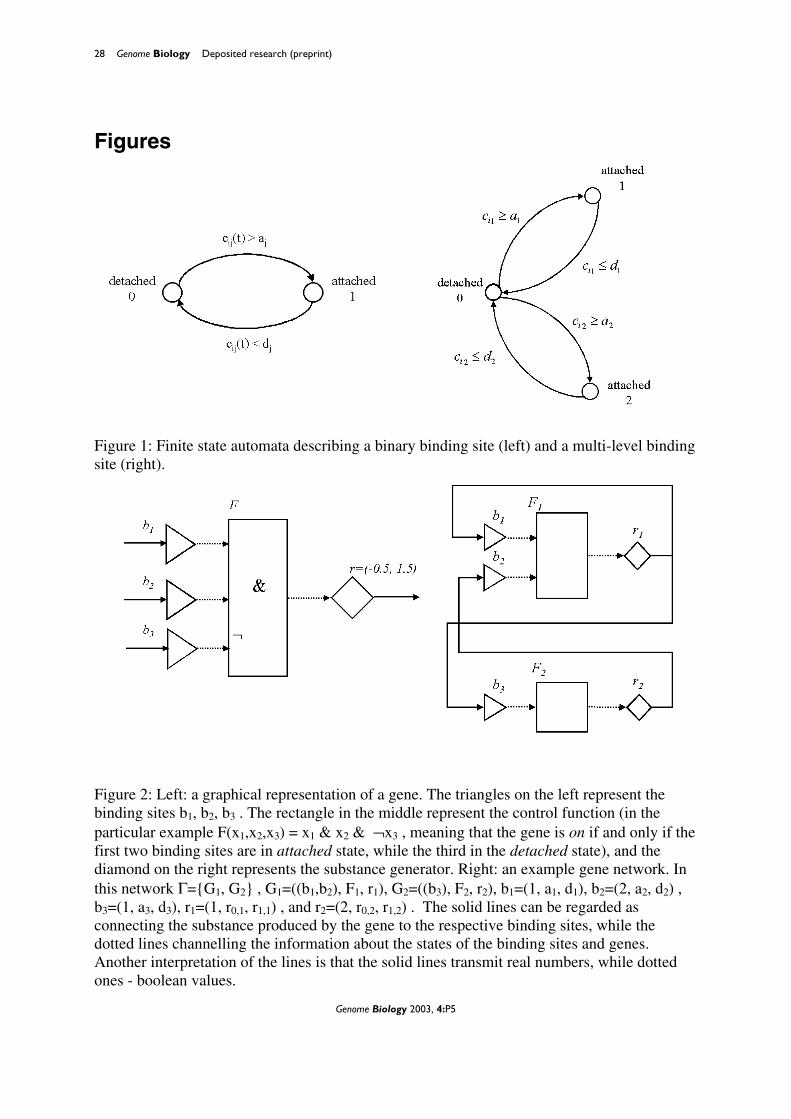
Figure 1: Finite state automata describing a binary binding site (left) and a multi-level binding site (right). Figure 2: Left: a graphical representation of a gene. The triangles on the left represent the binding sites b1, b2, b3 . The rectangle in the middle represent the control function (in the particular example F(x1,x2,x3) = x1 & x2 & ¬x3 , meaning that the gene is on if and only if the first two binding sites are in attached state, while the third in the detached state), and the diamond on the right represents the substance generator. Right: an example gene network. In this network Γ={G1, G2} , G1=((b1,b2), F1, r1), G2=((b3), F2, r2), b1=(1, a1, d1), b2=(2, a2, d2) , b3=(1, a3, d3), r1=(1, r0,1, r1,1) , and r2=(2, r0,2, r1,2) . The solid lines can be regarded as connecting the substance produced by the gene to the respective binding sites, while the dotted lines channelling the information about the states of the binding sites and genes. Another interpretation of the lines is that the solid lines transmit real numbers, while dotted ones - boolean values.



Figure 3: The functioning of a simple network of two binary genes with a negative feedback loop. Figure 4: The environment change graph

2

4

6

8

10

12

14

10 20 30 40 50 60 70 80 90 100

conc

entr

atio

n

Time

Genenet

a1d1

a2d2

a3d3

a4d4

Product 1Product 2

Figure 5: Left: Output of the simulation program “Genenet” (using Gnuplot for visualisation) Right: corresponding network; abbreviations: a1 stands for association constant 1, belongs to the bindingsite with the a1,d1 label, d1 is the corresponding dissociation constant; a2, d2, a3, d3, a4, d4 correspondingly



Figure 6: In-formal description of lambda-phage using the elements defined by our model (for further description see text)

N

cro/cIPL

cIIPE

PM

PE PcI cI

StrucPR’Q

intPint

cII

N xis

cIII

N

cI/cro

cI/cro

cI/cro

PM

Q

PRN

PR O

P

cro

cII

PQ

cIII

cII

cell

Other cII

stressOther cI

PL1 PL1

PL2 PL2

N

N

80%,100%

0%,100%

50%,100%

0%,100%

0,1,2,3

0,1,2

0,1,2,3,4,5,6

0,1,2,3

0,1

0,1,2

0,1

0,1

0,1,2

0,1,2

0,1,(2)

OR1

OR2

OR3



Figure 7: Simulation of lambda-phage model leading to lysogenic behaviour (top) or lytic behaviour (bottom)

0.00

1.00

2.00

3.13

3.33

3.55

4.00

4.22

4.67

4.88

5.33

5.55

6.00

6.22

6.67

6.88

7.33

7.55

8.00

8.22

8.67

8.88

9.33

9.55

cI

cII*

xis

cIII

Qcro

ON

int

0

5

10

15

20

25

con

cen

trat

ion

time

00.

9

1.5

1.9

2.4

2.7

3.05 3.3 4 5 6 7

7.55 8.5 9

10 11 12 13 14 15 16 17 18xis

cII*

cIII

Q

croO

Nint

cI

0

1

2

3

4

5

6

7

8

9

10

con

cen

trat

ion

time

xis

cII*

cIII

Q

cro

O

N

int

cI

lysis

lysogeny

Reverse Engineering of Gene Regulatory Network by Integration of Prior Global Gene Regulatory...

Documents

Transcript of Reverse Engineering of Gene Regulatory Network by Integration of Prior Global Gene Regulatory...