Biometrics DOI: 10.1111/biom.12309

Bayesian Nonlinear Model Selection for Gene Regulatory Networks

Yang Ni,1 Francesco C. Stingo,2,* and Veerabhadran Baladandayuthapani2

1Department of Statistics, Rice University, Houston, Texas, U.S.A.2Department of Biostatistics, The University of Texas MD Anderson Cancer Center, Houston, Texas, U.S.A.

∗email: fstingo@mdanderson.org

Summary. Gene regulatory networks represent the regulatory relationships between genes and their products and are impor-tant for exploring and defining the underlying biological processes of cellular systems. We develop a novel framework to recoverthe structure of nonlinear gene regulatory networks using semiparametric spline-based directed acyclic graphical models. Ouruse of splines allows the model to have both flexibility in capturing nonlinear dependencies as well as control of overfitting viashrinkage, using mixed model representations of penalized splines. We propose a novel discrete mixture prior on the smoothingparameter of the splines that allows for simultaneous selection of both linear and nonlinear functional relationships as well asinducing sparsity in the edge selection. Using simulation studies, we demonstrate the superior performance of our methodsin comparison with several existing approaches in terms of network reconstruction and functional selection. We apply ourmethods to a gene expression dataset in glioblastoma multiforme, which reveals several interesting and biologically relevantnonlinear relationships.

Key words: Directed acyclic graph; Gene regulatory network; Hierarchical model; MCMC; Model and functional selection;P-splines.

1. IntroductionA gene regulatory network (GRN) consists of a group of DNAsegments, such as genes and their products, and defines theirregulatory relationships at the cellular level. GRNs are in-structive for understanding complex biological processes andthe regulatory mechanisms underlying cellular systems. In thecontext of cancer, GRN reconstruction amongst key genes inthe signaling pathways helps to identify driver genes that di-rect carcinogenesis (Edelman et al., 2008), which then informsthe diagnosis and prognosis of the disease.

Our work is motivated by a study in glioblastomamultiforme (GBM), which is the most common and ag-gressive form of primary brain cancer in human adults.Due to its lethalness, GBM was the first cancer profiledby The Cancer Genome Atlas (TCGA) research network(http://cancergenome.nih.gov/). Intensive molecular studieshave identified three critical signaling pathways in humanglioblastomas (Furnari et al., 2007): (1) activation of the re-ceptor tyrosine kinase (RTK) and the phosphatidylinositol-3-OH kinase (PI3K) pathways; (2) inactivation of the p53pathway; and (3) inactivation of the retinoblastoma (Rb) tu-mor suppressor pathway. The fact that most of the GBM tu-mors possess abnormalities in all three of these core path-ways suggests they play a central role in the tumorigenesis ofGBM (Verhaak et al., 2010). In this work, we focus on mod-eling GRNs in GBM using expression data assayed on genesmapped to these core pathways. Our aims are not only to re-construct the underlying structure of the GRN, but also todiscover the functional nature of the dependencies betweenthe genes. A detailed description of the data is provided inSection 6.

Reverse engineering a GRN in a genomic context is knownto be challenging. This is partly due to high dimensional-ity since the graph space grows super-exponentially with thenumber of variables, making it computationally prohibitive touse exhaustive search algorithms over the entire graph space.More importantly, the interactions between genes may includenonlinear dependencies due to the complex biochemistry be-hind them (Kitano, 2002); therefore, models that rely on lin-ear assumptions may be inefficient in recovering the GRNs.In this article, we work with directed acyclic graphs (DAGs),which are powerful tools for recovering GRNs (Friedmanet al., 2000). DAGs, also known as Bayesian networks, aregraphs that consist of nodes representing random variables(genes in our case study) and directed edges representing con-ditional dependencies. DAGs are useful tools to apply whenwe construct networks from microarray expression data be-cause they are capable of detecting directed relationships andprovide a compact representation of the joint distribution,which leads to convenient modeling, computation and infer-ence.

Multiple methods based on DAGs have been proposed inthe literature in a variety of contexts. Friedman et al. (2000)developed DAGs from gene expression data using a bootstrap-based approach. Li, Yang, and Xing (2006) also constructedGRNs from expression microarray data wherein they esti-mated a linear Gaussian DAG model and computed the pre-cision matrix of the resulting joint distribution that definesan undirected graph. Stingo et al. (2010) proposed a DAG-based model to infer microRNA regulatory networks. Re-cently, Shojaie and Michailidis (2010) developed a penalizedlikelihood approach for estimating high-dimensional sparse

© 2015, The International Biometric Society 1

2 Biometrics

networks. Altomare, Consonni, and La Rocca (2013) proposedan objective Bayesian method for searching the DAG spacewith non-local priors. Fu and Zhou (2013) developed a pe-nalized likelihood method to recover causal DAGs from ex-perimental data. Some recent work includes the use of undi-rected graphical models to build biological networks (Petersonet al., 2013; Peterson, Stingo, and Vannucci, 2015). A commonthread underlying all these methods is that they allow for onlylinear dependencies between the nodes in the graph and donot explicitly incorporate nonlinear representations that maybe present in the data. In the GRN context, nonlinear depen-dencies may suggest some dynamic patterns of interactionsbetween genes, which could be the subject of further exper-imental validations. This is a gap in the literature that ourwork aims to fill. We develop a novel Bayesian framework forreconstructing GRNs based on the semiparametric estimationof DAGs. Our framework has four major innovations:

(1) Allows for the detection of interpretable nonlinear func-tional relationships between nodes using semiparamet-ric spline-based regressions.

(2) Enables explicit model selection and sparsity usingBayesian model selection techniques that resolve theissue of the number of parameters being larger thanthe sample size, while obtaining parsimonious repre-sentations.

(3) Uses a hierarchical two-level model selection approach.The first level is the edge selection, conditional on whichwe adopt the second level, functional selection, to clas-sify the degree of nonlinearity of the functional rela-tionship.

(4) Is computationally efficient since the regression setupallows for parallelizable estimations and the incorpo-ration of prior biological knowledge through referencenetworks to determine a priori the ordering of thegenes. This greatly reduces the complexity of the modeland the computational burden.

We evaluate the performance of our methods against thoseof alternative methods using simulations studies. Our meth-ods are very competitive in network structure recovery, re-construction of functional relationships and prediction. Wesubsequently apply our methods to the GBM data mentionedpreviously. While some of our results are consistent with pre-vious findings in the literature, we find new nonlinear inter-actions that are potential targets for future experimentationand validation. Although motivated by this specific gene ex-pression dataset, our approach is general and can be appliedto other scientific settings where such network-based inferenceis desirable.

2. Model

Let Y be an n × G matrix, where n is the number of samples

and G is the number of genes. Let y(l)g denote the expression

level of sample l and gene g, for g = 1, . . . , G and l = 1, . . . , n.A directed graph, also called a Bayesian network, G = {V, E}consists of a set V = {1, 2, . . . , G} of nodes, representing ran-dom variables {Y1, Y2, . . . , YG}, and a set E ⊆ {(i, j) : i, j ∈ V}of directed edges, representing the dependencies between the

nodes. Denote a directed edge from i to j by i → j where i

is a parent of j. The set of all the parents of j is denotedby pa(j). The absence of edges represents conditional inde-pendence assumptions. We restrict this work to DAGs, sincethere is no suitable well-defined joint distribution on cyclicgraphs (Whittaker, 2009). The joint distribution of a DAGcan be conveniently expressed as the product of the condi-tional distributions of each node given its parents:

P(Y1, . . . , YG) =G∏

g=1

P(Yg|Ypa(g)), (1)

where Ypa(g) = {Yj : j ∈ pa(g)}. Without loss of generality, theordering is defined as {1, 2, . . . , G}, which can be obtainedthrough prior biological knowledge such as known referencepathways. Within our DAG framework, biological knowledgeis then used to define the edge orientation such that gene i

can affect gene j for i < j, but not vice versa. Define [g−] to

be the set {1, 2, . . . , g − 1} and y(l)

[g−] to be {y(l)i : i ∈ [g−]}. Each

conditional distribution in the product term of equation (1)can be expressed by the following regressions:

y(l)g = fg(y

(l)

[g−]) + ε(l)g , g = 1, 2, . . . , G, l = 1, 2, . . . , n, (2)

where fg(y(l)

[g−]) is the predictor function and ε(l)g is the er-

ror, which is independently and normally distributed, ε(l)g ∼

N(0, λ−1g ).

Semiparametric modeling using penalized splines. In principle,fg(·) can be characterized using any nonlinear functional rep-resentation, depending on the context of the application. Forexample, if the relationship between genes follows a periodicor circadian pattern, one could choose fg(·) to be the Fourierbasis; similarly if the relationship follows a very localized(“spiky”) behavior, wavelets could potentially be employed.However, in the absence of such information a priori, wemodel fg(·) semiparametrically using a set of penalized splinebasis functions. Splines yield several advantages that includeflexibility as well as interpretability via representations thatuse a compact set of basis functions and coefficients. Moreimportantly, the inherent construction of penalized splines asmixed models with structured Gaussian priors on the coeffi-cients allows for analytical integration of the parameters (aswe show in Sections 4 and Web Appendix C), and thus allowsfor computational tractability. In particular, the predictor

fg(y(l)

[g−]) is modeled as the sum of the spline functions:

fg(y(l)

[g−]) = μg + fg,1(y(l)1 ) + fg,2(y

(l)2 )

+ · · · + fg,g−1(y(l)g−1), g = 1, . . . , G, (3)

where μg is the intercept for gene g and fg,i(·) =∑M

k=1β

(k)gi Bik(·), with Bik(·) being the kth cubic B-spline

basis. Let column vector βgj = (β(1)gj , β

(2)gj , . . . , β

(M)gj )′, col-

umn vector βg = (β′g1, β′

g2, . . . ,β′g,g−1)′, row vector Xlg =

(Bg1(y(l)g ), Bg2(y

(l)g ), . . . , BgM(y

(l)g )) and block matrix X = [Xlg]

Bayesian Nonlinear DAGs 3

with the (l, g)th block Xlg. Then model (3) can be written as

yg = μg + Xgβg + εg, g = 1, 2, . . . , G, (4)

where yg = (y(1)g , y

(2)g , . . . , y

(n)g )′, μg = μg1n, and εg =

(ε(1)g , ε

(2)g , . . . , ε

(n)g )′. Xg is the submatrix of X with the first

g − 1 column blocks. Combining equations (1), (2), and (4)yields the following likelihood function:

L =G∏

g=1

(λg

2π

) n2

exp{

−λg

2(yg − μg − Xgβg)

′(yg − μg − Xgβg)}

.

A key component in fitting splines is the choice of thenumber and the placement of knots (M). We address thisissue by using penalized splines (P-splines; Eilers and Marx,1996; Ruppert, Wand, and Carroll, 2003); wherein we choosea large enough number of knots that are sufficient to capturethe local nonlinear features present in the data and control foroverfitting by using a penalty matrix on the basis coefficients.Under the Bayesian framework, the penalties can be repre-sented using Gaussian random walk priors (Lang and Brezger,2004; Baladandayuthapani, Mallick, and Carroll, 2005) onthe spline coefficients, βgj|τgj, λg ∼ N(0, (τgjλgK)−1), whereτgj is the smoothing parameter and K is the penalty matrix.We construct K from the second order differences of theadjacent spline coefficients, namely, β

(k+1)gj − 2β

(k)gj + β

(k−1)gj

(Lang and Brezger, 2004), which can be construed as a“roughness penalty.” Note that in the above construction,the degree of smoothness of the fitted curve is controlled bythe smoothing parameters, τgj. A large value of τgj, that is,a strong roughness penalty, leads to a smoother fit, while asmall value of τgj (close to zero) leads to an irregular fit andessentially interpolation of the data.

3. Model Selection

In this section, we introduce our hierarchical two-level selec-tion on the edges as well as the functional form of the selectededges.First-level selection: “Edge selection.” Our goal is to infer thestructure of the GRN; inference on the predictor functions,defined in equation (3), will automatically lead to the selec-tion of the relevant connections. An important aspect of ourmethodology is sparsity, that is, we believe that most of thegene–gene associations are almost negligible. To this end, wetake a Bayesian model selection approach that allows for theselection of edges supported by the data. More importantly,model selection is desirable when the number of parameters tobe estimated, 2G + G(G−1)

2M in our case, is much larger than

the sample size, even for a moderate number of genes. Forexample, in our real data analysis, the number of parametersis more than 12,000 while the sample size is about 250.

Here, model selection is achieved through a mixture prioron the spline coefficients, where the first component isthe second-order Gaussian random walk described in Sec-tion 2 and the second component is the point mass at 0,which is expressed as βgj|τgj, λg, γgj ∼ γgjN(0, (τgjλgK)−1) +(1 − γgj)δ0(βgj), where δ0 is the Dirac delta function. The bi-nary indicators, γgj, are latent variables that encode the struc-

ture of the network. If γgj = 1, the arrow from gene j to geneg (j → g) is included in the network, and γgj = 0 otherwise.

The smoothing parameter τgj controls the smoothness ofthe fitted curve, and small values of τgj lead to an unde-sirable irregular fit. The conjugate Gamma prior is right-skewed, which puts a lot of mass around zero; therefore,this standard prior (Lang and Brezger, 2004) is consideredinappropriate in this setting where regularized fits are re-quired for multiple regressions. Instead, we assume an in-verted Pareto prior Ip(aτ, bτ) for the smoothing parameter(Morrissey et al., 2011), which takes the form π(τ|a, b) =a

b( τ

b)a−1, for a > 0, 0 < τ < b. Contrary to that of Gamma

distributions, the skewness of inverted Pareto distributions iseasily adjusted through parameter a. This prior concentrateson large values when a > 1, and then encourages smooth fitsof the data, which are desired in our scenario. See further de-tailed discussions in Web Appendix A. We refer to this modelthat has an absolutely continuous inverted Pareto prior onthe smoothing parameter as the nonlinear DAG (nDAG).Second-level selection: “Functional selection.” In addition toedge selection (i.e., presence/absence of an edge), we are alsointerested in the functional nature of the interactions (i.e., lin-ear or nonlinear) and let the data dictate this choice. We pro-pose a hierarchical second-level selection technique, whereinconditional on γgj, the functional form of the relationship be-tween genes is defined through τgj, as these parameters controlthe smoothness of the curve fitting. We enforce a discrete mix-ture of the inverted Pareto distribution and Gamma distri-bution: τgj|φgj ∼ φgjGamma(kτ, θτ) + (1 − φgj)Ip(aτ, bτ), whereφgj is the indicator of the mixture component. The Gammadistribution is concentrated at small values of τ, thus inducingnonlinear smoothing; whereas the inverted Pareto distributionplaces its mass on large values (i.e., setting aτ > 1), thus lead-ing to a more linear fit. Unlike a unimodal prior (such as theGamma and inverted Pareto distributions), which is concen-trated at either small values or large values (but not both),this mixture prior provides a sharper separation between “lin-ear” and “nonlinear” relationships among genes because of itsbimodal nature. One example of such a mixture prior is shownin Web Figure 3. In essence, φgj = 1 implies a nonlinear inter-action between gene g and gene j; whereas φgj = 0 implies alinear interaction. The elicitation of this mixture prior is de-tailed in Web Appendix B. We call this the nonlinear mixtureDAG (nMixDAG) so as to distinguish it from the nDAG.

4. Hyper-Prior Specifications

In this section, we complete the hierarchical formulation ofour model by specifying the hyper-prior on the precision oferror term λg, constant term μg, network parameter γgj andits hyperparameter ρ, and the mixture component indicatorφgj and its hyperparameter ω.

We assume conjugate priors for the error precision λg ∼Gamma(aλ, bλ) and the constant term μg ∼ N(0, (λgκμ)−1).For the network parameter γgj, we use a Bernoulli priorwith success probability ρ, γgj|ρ ∼ Bernoulli(ρ). The priorprobability of inclusion ρ follows a Beta distribution, ρ ∼Beta(aρ, bρ), which yields an automatic multiplicity penaltysince the posterior distribution of ρ will become more con-centrated at small values near 0 as the total number of

4 Biometrics

Figure 1. Schema of the nonlinear mixture directed acyclic graphical model. Model parameters/random variables are incircles and model constants/data are in boxes.

variables increases (Scott and Berger, 2010). Similar to theprior for γgj, a Bernoulli distribution is assumed for φgj,with the success probability following a Beta hyper-prior,φgj|ω ∼ Bernoulli(ω), ω ∼ Beta(aω, bω). A schematic repre-sentation of the complete hierarchical formulation is shownin Figure 1. In Web Appendix C, we present the details of theposterior inference and MCMC sampling scheme.

5. Simulated Examples

In this section, we illustrate our proposed methods with sim-ulated examples. We design five scenarios with 150 samples,50 genes and 100 connections, and run 50 simulations for eachscenario. Although the number of genes is less than the samplesize, using the spline basis expansions, the number of effec-tive estimable parameters is 12,350 for the saturated model,which greatly exceeds the sample size. The five scenarios dif-fer in the percentage of linearity in the data (0%, 20%, 48%,72%, and 100%), corresponding to the proportion of the linearfunctions that generate the data. The structure of the networkis assumed to be constant across all simulations. Error termsare distributed as N(0, 42).

We use a cubic B-spline with 6 interior knots, that is,10 bases. For the nDAG, the prior parameters are specifiedas κμ = 1/4, (aλ, bλ) = (2, 1), (aρ, bρ) = (2, 2), and (aτ, bτ) =(1.5, 400). For the additional parameter in the nMixDAG, welet (aω, bω) = (2, 2), and (kτ, θτ) = (3, 2). The choice of thesehyperparameters aims to be mainly non-informative. We pro-vide a sensitivity analysis on the prior specifications at theend of this section. The results show a very low sensitivityto these choices. We run an MCMC algorithm with 20,000iterations, in which the first 2000 iterations are considered asa “burn-in” period for both methods.

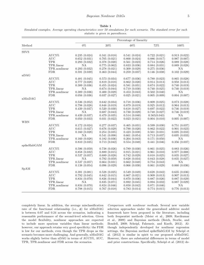
Since the true simulated network is known, we can computethe operating characteristics of the methods using the truepositive rate (TPR), the false discovery rate (FDR) and thearea under the receiver operating characteristic (ROC) curve(AUC). We also compute the TPR separately for the linearand nonlinear relationships, which we refer to as TPR linearand TPR nonlinear, respectively. In addition, while the fullAUC indicates the overall performance of the underlyingmethod, researchers may be particularly interested in the per-formance with a controlled false positive rate (FPR), say, lessthan 5%; hence, we also report the partial AUC truncated atFPR< 5%, denoted by AUC5%. All the statistics mentionedabove are summarized in Table 1. A separate simulation studyon variable selection under the generalized additive model set-ting with varying sample sizes and signal-to-noise ratios isprovided in Web Appendix D.Comparison with linear methods. We consider two linearmethods for comparison: (1) the linear model selectionmethod (George and McCulloch, 1993; Marin and Robert,2007), referred to as SSVS; and (2) the ordering-free Bayesiannetwork (WBN) approach that follows the implementationof Werhli, Grzegorczyk, and Husmeier (2006), which hasbeen shown by Allen et al. (2012) to outperform competingordering-free Bayesian network methods. In each of the fivescenarios, our methods outperform both SSVS and WBN.For example, when the true model is completely nonlinear,the AUC of the SSVS is as low as 0.652, while the AUC of thenMixDAG is 0.798. The TPRs of WBN are always lower thanthose of the other three methods, while the FDRs are alwayshigher. As expected, the performance of the SSVS is closerto those of our methods when the linearity increases, andSSVS slightly outperforms our methods when the data are

Bayesian Nonlinear DAGs 5

Table 1Simulated examples. Average operating characteristics over 50 simulations for each scenario. The standard error for each

statistic is given in parentheses.

Percentage of linearity

Method 0% 20% 48% 72% 100%

SSVSAUC5% 0.235 (0.024) 0.341 (0.018) 0.541 (0.024) 0.722 (0.021) 0.913 (0.022)AUC 0.652 (0.031) 0.705 (0.021) 0.800 (0.024) 0.886 (0.017) 0.987 (0.007)TPR 0.293 (0.032) 0.378 (0.020) 0.561 (0.023) 0.714 (0.026) 0.889 (0.028)TPR linear NA 0.775 (0.062) 0.833 (0.036) 0.884 (0.031) 0.889 (0.028)TPR nonlinear 0.293 (0.032) 0.278 (0.021) 0.309 (0.029) 0.275 (0.036) NAFDR 0.591 (0.039) 0.463 (0.044) 0.259 (0.037) 0.146 (0.038) 0.102 (0.029)

nDAGAUC5% 0.481 (0.045) 0.573 (0.034) 0.677 (0.036) 0.788 (0.023) 0.865 (0.028)AUC 0.777 (0.028) 0.819 (0.018) 0.862 (0.020) 0.914 (0.013) 0.958 (0.013)TPR 0.389 (0.036) 0.455 (0.024) 0.581 (0.031) 0.674 (0.022) 0.740 (0.019)TPR linear NA 0.674 (0.044) 0.719 (0.030) 0.740 (0.025) 0.740 (0.019)TPR nonlinear 0.389 (0.036) 0.400 (0.029) 0.453 (0.043) 0.502 (0.040) NAFDR 0.056 (0.036) 0.037 (0.027) 0.025 (0.021) 0.005 (0.009) 0.004 (0.007)

nMixDAGAUC5% 0.536 (0.052) 0.642 (0.034) 0.718 (0.036) 0.809 (0.025) 0.873 (0.028)AUC 0.798 (0.028) 0.848 (0.019) 0.879 (0.019) 0.925 (0.012) 0.964 (0.013)TPR 0.439 (0.037) 0.520 (0.030) 0.618 (0.027) 0.697 (0.022) 0.746 (0.019)TPR linear NA 0.687 (0.043) 0.730 (0.029) 0.748 (0.027) 0.746 (0.019)TPR nonlinear 0.439 (0.037) 0.479 (0.035) 0.514 (0.040) 0.565(0.043) NAFDR 0.050 (0.033) 0.031 (0.022) 0.023 (0.021) 0.004 (0.010) 0.005 (0.007)

WBNAUC5% 0.172 (0.024) 0.277 (0.037) 0.465 (0.031) 0.599 (0.030) 0.751 (0.037)AUC 0.615 (0.027) 0.676 (0.029) 0.790 (0.020) 0.862 (0.022) 0.901 (0.023)TPR 0.160 (0.028) 0.254 (0.035) 0.423 (0.038) 0.561 (0.031) 0.695 (0.033)TPR linear NA 0.541 (0.098) 0.661 (0.054) 0.713 (0.037) 0.695 (0.033)TPR nonlinear 0.160 (0.028) 0.182 (0.036) 0.204 (0.043) 0.171 (0.050) NAFDR 0.810 (0.035) 0.713 (0.042) 0.554 (0.048) 0.441 (0.046) 0.356 (0.037)

spikeSlabGAMAUC5% 0.596 (0.059) 0.738 (0.026) 0.789 (0.030) 0.861 (0.025) 0.883 (0.026)AUC 0.858 (0.032) 0.889 (0.015) 0.915 (0.021) 0.961 (0.010) 0.977 (0.008)TPR 0.537 (0.057) 0.689 (0.028) 0.742 (0.029) 0.818 (0.025) 0.835 (0.027)TPR linear NA 0.792 (0.059) 0.828 (0.034) 0.843 (0.028) 0.835 (0.027)TPR nonlinear 0.537 (0.057) 0.664 (0.031) 0.662 (0.048) 0.754 (0.043) NAFDR 0.138 (0.054) 0.096 (0.029) 0.066 (0.030) 0.061 (0.029) 0.060 (0.036)

SpAMAUC5% 0.391 (0.081) 0.528 (0.025) 0.549 (0.049) 0.628 (0.042) 0.635 (0.036)AUC 0.792 (0.045) 0.842 (0.015) 0.867 (0.021) 0.909 (0.013) 0.907 (0.013)TPR 0.834 (0.070) 0.826 (0.044) 0.870 (0.036) 0.887 (0.026) 0.887 (0.029)TPR linear NA 0.835 (0.071) 0.892 (0.045) 0.894 (0.032) 0.887 (0.029)TPR nonlinear 0.834 (0.070) 0.824 (0.046) 0.850 (0.042) 0.871 (0.046) NAFDR 0.798 (0.015) 0.767 (0.018) 0.783 (0.014) 0.774 (0.015) 0.776 (0.013)

completely linear. In addition, the average misclassificationrate of the functional relationship (i.e., φ) for nMixDAGis between 0.07 and 0.24 across the scenarios, indicating areasonable performance of the second-level selection. Giventhe model flexibility, nonlinear approaches are expectedto include more spurious variables than linear methods;however, our approach retains very good specificity: the FDRis low for our methods, even though the TPR drops as thescenario becomes more challenging. And generally, nMixDAGworks slightly better than nDAG in terms of AUC5%, AUC,TPR, TPR nonlinear and FDR across the scenarios.

Comparison with nonlinear methods. Several new variableselection approaches under the generalized additive modelframework have been proposed in the literature, includingboth frequentist methods (Meier et al., 2009; Ravikumaret al., 2009) and Bayesian methods (Reich, Storlie, andBondell, 2009; Scheipl, Fahrmeir, and Kneib, 2012). Al-though independently developed for nonlinear regressionsettings, the Bayesian method spikeSlabGAM by Scheipl etal. (2012) is similar in spirit to our proposed nMixDAG.However, there are substantial differences in terms of modeland prior constructions. Specifically, Scheipl et al. (2012) de-

6 Biometrics

Table 2Simulated examples. Sensitivity of nMixDAG to misspecified ordering of the nodes. The standard error for each statistic is

given in parentheses.

Method nMixDAG WBN

Kendall’s tau 0.00 0.25 0.51 1.00V-structures (assumed) 124 146 138 159V-structures (shared) 124 87 23 0AUC5% 0.718 (0.036) 0.603 (0.031) 0.468 (0.023) 0.424 (0.023) 0.537 (0.022)AUC 0.879 (0.019) 0.838 (0.019) 0.785 (0.016) 0.765 (0.018) 0.809 (0.018)TPR 0.618 (0.027) 0.534 (0.031) 0.456 (0.026 ) 0.374 (0.022) 0.551 (0.027)TPR linear 0.730 (0.029) 0.651 (0.040) 0.595 (0.045) 0.506 (0.047) 0.806 (0.041)TPR nonlinear 0.514 (0.040) 0.425 (0.039) 0.328 (0.023) 0.252 (0.024) 0.316 (0.035)FDR 0.023 (0.021) 0.102 (0.033) 0.240 (0.034) 0.242 (0.044) 0.420 (0.033)

composed the spline design matrix into unpenalized andpenalized parts through spectral decomposition, which yieldsan orthogonal basis representation; whereas we directly workwith spline basis functions. For model/variable selection,they imposed a spike-and-slab prior on the hyper-variance ofthe regression coefficients; whereas our approach introducesspike-and-slab priors with a point mass at zero directly onthe regression coefficients. Together, these changes inducedifferent shrinkage and selection properties for nonlinearregression in general and DAG models in particular, as wedemonstrate via simulations and real data analysis. Here, wecompare nMixDAG with spikeSlabGAM and the frequentistmethod SpAM (Ravikumar et al., 2009) in the contextof nonlinear DAGs. Although Ravikumar et al. (2009)recommended choosing the tuning parameter of SpAM viageneralized cross-validation, we picked the tuning parametervia 10-fold cross-validation as this approach resulted inbetter performances in our simulation studies.

Our methods show very competitive performance. The fre-quentist approach SpAM always has higher TPR than ourmethods and spikeSlabGAM, however it is achieved at thecost of unacceptably high FDR and hence it has the low-est AUC and AUC5%. For the Bayesian methods, we do notobserve a statistically significant difference in all character-istics. For example, in scenario 3, the difference in AUC fornMixDAG and spikeSlabGAM is only 0.036, while their stan-dard errors are 0.019 and 0.021. The AUCs are within twostandard deviations of each other; hence, the difference is notsignificant. In Web Figure 7, we plot the ROC curves of thethree nonlinear methods for one randomly selected simula-tion from scenario 3. There is a trade-off between TPR andFDR for the two competing methods. For instance, in sce-nario 1, the TPRs are 0.439 and 0.537 and the FDRs are0.050 and 0.138 for nMixDAG and spikeSlabGAM, respec-tively. The low FDRs are particularly useful in a genomiccontext as the selected genes are typically targets of furthervalidation via biological experiments. Hence, a parsimoniousapproach will probably save on research expenses and time.Sensitivity analysis of ordering misspecification. The majorassumption of our methods is the known prior ordering ofthe variables. When such ordering is available, this assump-tion is advantageous, as we have seen that our methods out-perform the ordering-free WBN in all scenarios (Table 1).However, in some applications, the ordering may be partially

known or not known at all. Under such circumstances, wewould like to investigate the robustness of our methods com-pared to WBN. We follow the ideas of Shojaie and Michailidis(2010) and Altomare et al. (2013) and perform a sensitivityanalysis of nMixDAG to different ordering misspecifications.The performance of our method depends on the distance be-tween the true ordering and the assumed ordering, and thenumber of v-structures (i.e., i → j ← k) for both the true or-dering and the assumed ordering. To quantify this distance,we use the normalized Kendall’s tau distance, which is de-fined as the ratio of the number of discordant pairs over thetotal number of pairs. The normalized Kendall’s tau distancelies between 0 and 1, with 0 indicating a perfect agreementof the two orderings and 1 indicating a perfect disagreement.Since our method is not able to learn the ordering, we evalu-ate the performance of our method based on only the skeletonof the true graph (i.e., the directions of the edges are ignored).We pick scenario 3 and shuffle the data according to the or-derings with different normalized Kendall’s tau distances. InTable 2, we list normalized Kendall’s tau distances, the num-ber of v-structures of the assumed ordering, the number ofshared v-structures between the true and the assumed order-ings, TPR, TPR linear, TPR nonlinear, and FDR for bothnMixDAG and WBN. When there is moderate misspecifica-tion (Kendall’s tau=0.25), nMixDAG outperforms WBN interms of AUC (0.838 vs. 0.809) and remarkably FDR (0.102vs. 0.420). When Kendall’s tau is 0.51 or even 1.00, nMixDAGstill has a surprisingly reasonable AUC (0.785 and 0.765,respectively) that is just slightly lower than that of WBN(0.809), and a very good control of FDR (0.240 and 0.242,respectively), which is much lower than that of WBN (0.420).Performance in high-dimensional settings. We investigate thescalability of nMixDAG, setting the number of genes atG = 100, 150, 200 while keeping the number of connectionsfixed. With G = 200 and M = 10 bases, we have approxi-mately 200,000 parameters to estimate already given the non-linear and network construction. We again pick scenario 3 (re-sults shown in Web Table 2). The performance of nMixDAGis almost invariant with respect to the dimensions. As the di-mension increases, TPR and AUC slightly decrease, but FDRalso decreases. Computationally, the running time increasesvery slowly with the dimension. On a single AMD 6174 pro-cessor, the average computation times are 1.4, 1,8, 2.2, and2.7 hours for G = 50, 100, 150, 200, respectively.

Bayesian Nonlinear DAGs 7

Sensitivity analysis of hyperparameter settings. We conducta series of analyses to test the sensitivity of our method todifferent prior specifications. We pick scenario 3 as a repre-sentative case since it has about 50% linear functions, andshow our results for nMixDAG. In Web Table 3 and Web Ta-ble 4, we report the performance under different hyper-priorspecifications for ρ and τ, all of which demonstrate that theperformance of our method is quite stable.

6. Data Analysis: GBM Data

We apply our methods to analyze TCGA-based GBM geneexpression data, as introduced in Section 1. TCGA providesmicroarray-based gene expression data for a large cohort ofGBM tumor specimens (241 in our case study) (TCGA, 2008).Among more than 10,000 genes in the raw data, we focus ouranalysis on 49 genes that overlap with the three critical signal-ing pathways (Furnari et al., 2007), the RTK/PI3K signalingpathway, p53 signaling pathway, and Rb signaling pathway.A better understanding of the GRN will provide new insightsinto the tumorigenesis of GBM (Verhaak et al., 2010).

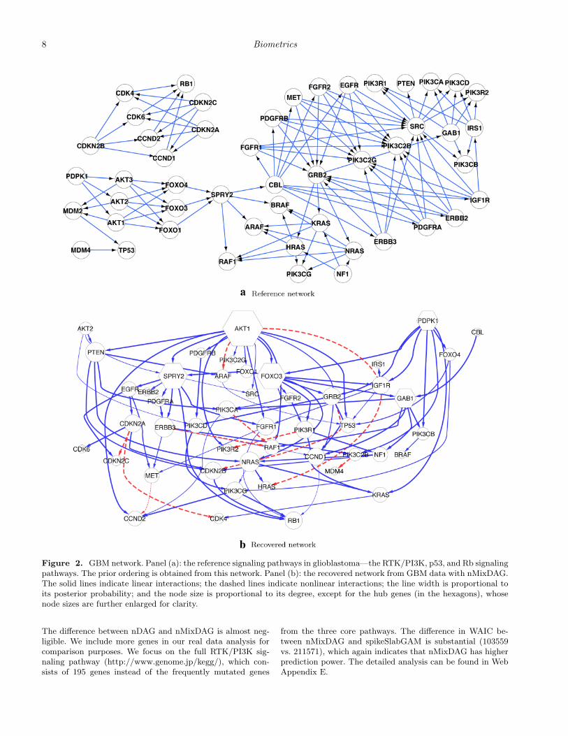
We assume the same prior specifications as in Section 5.Our reference network is the induced subgraph of the signal-ing pathways in glioblastoma from TCGA (2008), as shownin Figure 2(a), from which we obtain our prior ordering. Werun two separate MCMC chains with different starting val-ues, each with 20,000 iterations. For convergence diagnos-tics, we examine all the parameters that we sample from theMCMC algorithm. In particular, we calculate the Gelman–Rubin potential scale reduction factor (PSRF, Gelman andRubin (1992)) for the continuous parameters τgj (ranging from1.000 to 1.026) and ρ (1.000 and 1.001 for nMixDAG andnDAG, respectively). For the discrete parameter γ, the corre-lation between the posterior probabilities of the two chains is0.994 for nMixDAG and 0.995 for nDAG. For the additionalparameters of nMixDAG, φ and ω, the correlation and PSRFare 0.988 and 1.000, respectively. All the PSRFs and correla-tions are very close to 1, which is indicative of good mixing ofthe MCMC chain, as well as its convergence to the stationaryregion. The computation time is 1.9 hours on a 3.5 GHz IntelCore i7 processor. We combine the two chains and discard thefirst 10% of the iterations of each chain as a burn-in.

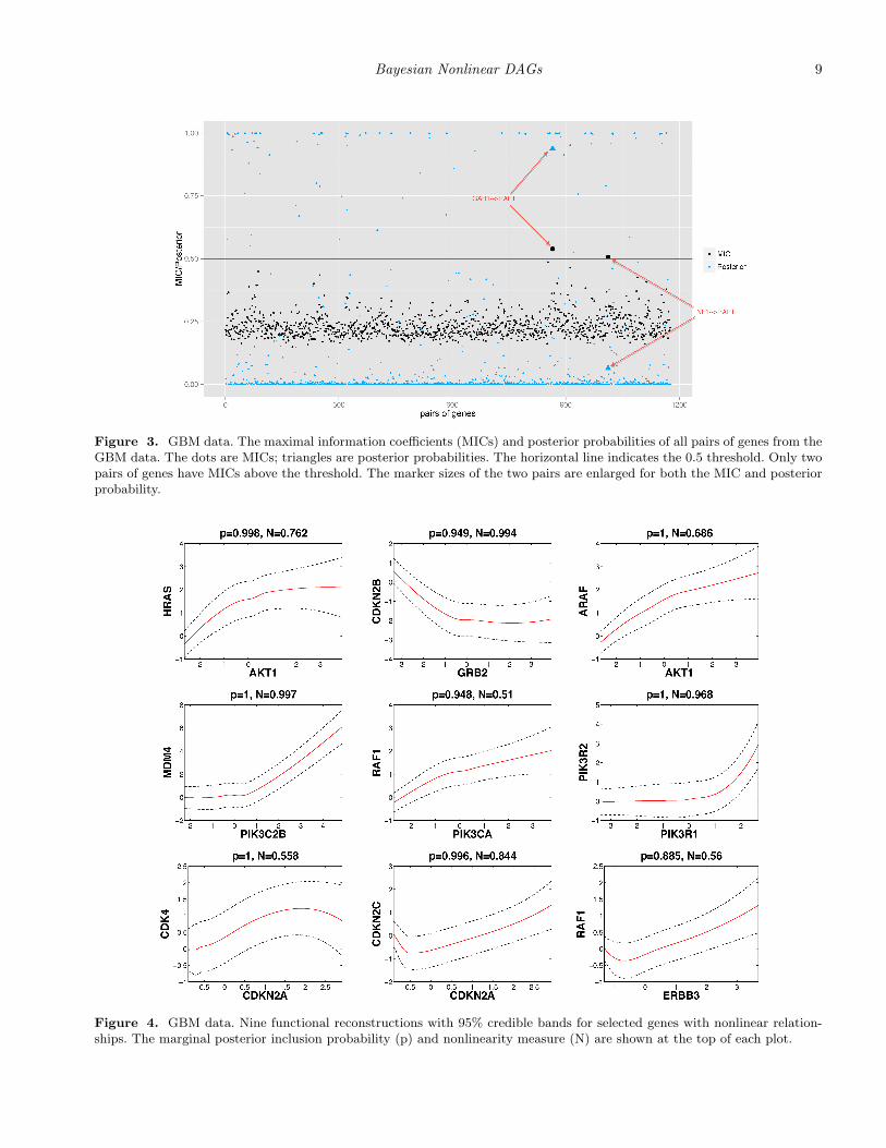
Figure 2(b) shows the network recovered by nMixDAG. Thesolid lines indicate linear interactions and the dashed lines in-dicate nonlinear interactions. The line width is proportionalto the posterior probability, with thicker lines indicating ahigher probability of the edge, and the node size is propor-tional to its degree, that is, the number of edges connectedto the node. A heat map of the marginal posterior inclusionprobability of each edge is provided in Web Figure 5 (WebAppendix E). In total, we find 95 connections, of which 85are linear and 10 are nonlinear. While we find several novelconnections, some of our findings are consistent with knowninteractions reported in the biological literature. For instance,our study confirms that in the cytoplasm, the NF1 proteininhibits RAS function (Malumbres and Barbacid, 2003) andRAS proteins activate PI3K complexes (Blume-Jensen andHunter, 2001). We also calculate the maximal information co-efficient (MIC) (Reshef et al., 2011), as this approach has beenwidely used in the analysis of genomic data. The MIC mea-

sures the pairwise linear or nonlinear association by mutualinformation on continuous random variables for the 49 genesof interest (totaling 1176 pairs). The MICs are represented bydots in Figure 3. We find only two pairs of genes with MICslarger than 0.5: GAB1 → RAF1 and NF1→ RAF1, of whichGAB1→RAF1 is also detected by our methods. The trianglesare the posterior probabilities of the inclusion of gene pairs bynMixDAG, and the horizontal line is the 0.5 threshold. Theenlarged markers are the pairs of genes for which the MICsare higher than the 0.5 threshold. This indicates that meth-ods that estimate marginal nonlinear correlations, such as theMIC approach, may miss some relevant connections that areprovided by the nonlinear graphical models. In addition, theMIC approach does not explicitly identify the formal rela-tionships; whereas our approach does this from a functionalreconstruction.

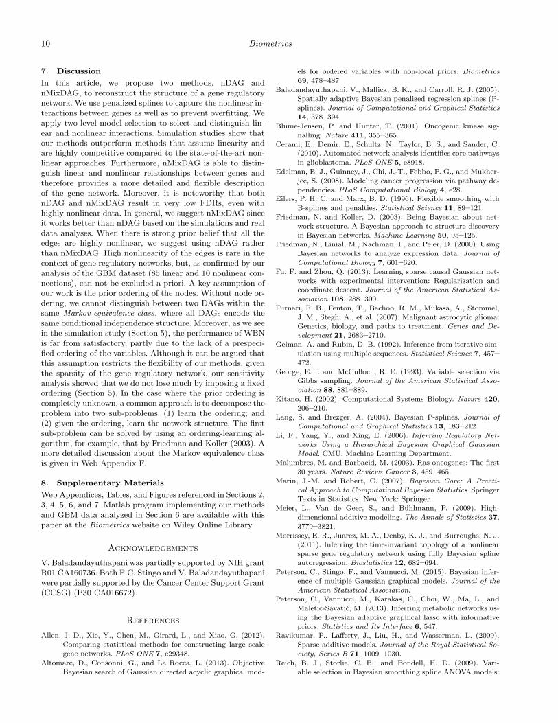
Based on the recovered network in Figure 2, several hubgenes are identified: AKT1, FOXO3, SPRY2, GAB1, andPDPK1, with degrees of 15, 10, 10, 7, and 7, respectively. Hubgenes are of particular interest as potential major drivers ofdisease etiology because they are often more involved in mul-tiple regulatory activities than non-hub genes. All the five hubgenes we find have been previously identified as driver genes(Cerami et al., 2010), and are significantly altered in GBM, forexample, the AKT family is often amplified, while the FOXOfamily is frequently mutated (TCGA, 2008) in GBM. We alsoplot the nonlinear functional reconstructions of nine edges,together with their 95% credible bands in Figure 4. Marginalposterior inclusion probabilities are shown on the top of eachplot. We can see that the expression level of RAF1 decreaseswith that of ERBB3 when ERBB3 is low in expression, butstarts to increase with ERBB3 after a cut-point around −0.7.It is even more interesting that CDKN2A manifests a sinu-soidal trend with CDK4. These relationships have not beenreported previously to the best of our knowledge and maydeserve further validation via biological experiments.

We define the nonlinearity measure (N) as Ngj = p(φgj =1|Y , γgj = 1), the probability that a given connection (γgj = 1)is nonlinear (φgj=1) a posteriori, which can be easily com-

puted from MCMC samples of φgj, γgj: Ngj ≈ ∑N

i=1I(φ

(i)gj =

1, γ(i) = γ select , γ(i)gj = 1)/

∑N

i=1I(γ(i) = γ select , γ

(i)gj = 1) where

the superscript (i) labels the ith MCMC sample, N is thenumber of MCMC samples and γ select indicates the selectedγ from the highest posterior model. This measure quantifiesthe evidence for the nonlinearity of each curve reconstructedin Figure 4 (shown on the top of each plot). For example,the evidence for nonlinearity between PIK3C2B and MDM4is strong (0.997), while the evidence between PIK3CA andRAF1 is much weaker (0.510), which is consistent with ourobservations.

For comparison, we apply spikeSlabGAM to the GBM dataand evaluate the performance via the widely applicable in-formation criterion (WAIC) of Watanabe (2010), which isa fully Bayesian predictive information criterion based onthe point-wise posterior predictive density and is asymptot-ically equal to Bayesian leave-one-out cross-validation. Ourmethods, nDAG and nMixDAG, have lower WAICs thanspikeSlabGAM (27378 and 27413 vs. 32579), which is in-dicative of better prediction performance by our methods.

8 Biometrics

Figure 2. GBM network. Panel (a): the reference signaling pathways in glioblastoma—the RTK/PI3K, p53, and Rb signalingpathways. The prior ordering is obtained from this network. Panel (b): the recovered network from GBM data with nMixDAG.The solid lines indicate linear interactions; the dashed lines indicate nonlinear interactions; the line width is proportional toits posterior probability; and the node size is proportional to its degree, except for the hub genes (in the hexagons), whosenode sizes are further enlarged for clarity.

The difference between nDAG and nMixDAG is almost neg-ligible. We include more genes in our real data analysis forcomparison purposes. We focus on the full RTK/PI3K sig-naling pathway (http://www.genome.jp/kegg/), which con-sists of 195 genes instead of the frequently mutated genes

from the three core pathways. The difference in WAIC be-tween nMixDAG and spikeSlabGAM is substantial (103559vs. 211571), which again indicates that nMixDAG has higherprediction power. The detailed analysis can be found in WebAppendix E.

Bayesian Nonlinear DAGs 9

Figure 3. GBM data. The maximal information coefficients (MICs) and posterior probabilities of all pairs of genes from theGBM data. The dots are MICs; triangles are posterior probabilities. The horizontal line indicates the 0.5 threshold. Only twopairs of genes have MICs above the threshold. The marker sizes of the two pairs are enlarged for both the MIC and posteriorprobability.

Figure 4. GBM data. Nine functional reconstructions with 95% credible bands for selected genes with nonlinear relation-ships. The marginal posterior inclusion probability (p) and nonlinearity measure (N) are shown at the top of each plot.

10 Biometrics

7. Discussion

In this article, we propose two methods, nDAG andnMixDAG, to reconstruct the structure of a gene regulatorynetwork. We use penalized splines to capture the nonlinear in-teractions between genes as well as to prevent overfitting. Weapply two-level model selection to select and distinguish lin-ear and nonlinear interactions. Simulation studies show thatour methods outperform methods that assume linearity andare highly competitive compared to the state-of-the-art non-linear approaches. Furthermore, nMixDAG is able to distin-guish linear and nonlinear relationships between genes andtherefore provides a more detailed and flexible descriptionof the gene network. Moreover, it is noteworthy that bothnDAG and nMixDAG result in very low FDRs, even withhighly nonlinear data. In general, we suggest nMixDAG sinceit works better than nDAG based on the simulations and realdata analyses. When there is strong prior belief that all theedges are highly nonlinear, we suggest using nDAG ratherthan nMixDAG. High nonlinearity of the edges is rare in thecontext of gene regulatory networks, but, as confirmed by ouranalysis of the GBM dataset (85 linear and 10 nonlinear con-nections), can not be excluded a priori. A key assumption ofour work is the prior ordering of the nodes. Without node or-dering, we cannot distinguish between two DAGs within thesame Markov equivalence class, where all DAGs encode thesame conditional independence structure. Moreover, as we seein the simulation study (Section 5), the performance of WBNis far from satisfactory, partly due to the lack of a prespeci-fied ordering of the variables. Although it can be argued thatthis assumption restricts the flexibility of our methods, giventhe sparsity of the gene regulatory network, our sensitivityanalysis showed that we do not lose much by imposing a fixedordering (Section 5). In the case where the prior ordering iscompletely unknown, a common approach is to decompose theproblem into two sub-problems: (1) learn the ordering; and(2) given the ordering, learn the network structure. The firstsub-problem can be solved by using an ordering-learning al-gorithm, for example, that by Friedman and Koller (2003). Amore detailed discussion about the Markov equivalence classis given in Web Appendix F.

8. Supplementary Materials

Web Appendices, Tables, and Figures referenced in Sections 2,3, 4, 5, 6, and 7, Matlab program implementing our methodsand GBM data analyzed in Section 6 are available with thispaper at the Biometrics website on Wiley Online Library.

Acknowledgements

V. Baladandayuthapani was partially supported by NIH grantR01 CA160736. Both F.C. Stingo and V. Baladandayuthapaniwere partially supported by the Cancer Center Support Grant(CCSG) (P30 CA016672).

References

Allen, J. D., Xie, Y., Chen, M., Girard, L., and Xiao, G. (2012).Comparing statistical methods for constructing large scalegene networks. PLoS ONE 7, e29348.

Altomare, D., Consonni, G., and La Rocca, L. (2013). ObjectiveBayesian search of Gaussian directed acyclic graphical mod-

els for ordered variables with non-local priors. Biometrics69, 478–487.

Baladandayuthapani, V., Mallick, B. K., and Carroll, R. J. (2005).Spatially adaptive Bayesian penalized regression splines (P-splines). Journal of Computational and Graphical Statistics14, 378–394.

Blume-Jensen, P. and Hunter, T. (2001). Oncogenic kinase sig-nalling. Nature 411, 355–365.

Cerami, E., Demir, E., Schultz, N., Taylor, B. S., and Sander, C.(2010). Automated network analysis identifies core pathwaysin glioblastoma. PLoS ONE 5, e8918.

Edelman, E. J., Guinney, J., Chi, J.-T., Febbo, P. G., and Mukher-jee, S. (2008). Modeling cancer progression via pathway de-pendencies. PLoS Computational Biology 4, e28.

Eilers, P. H. C. and Marx, B. D. (1996). Flexible smoothing withB-splines and penalties. Statistical Science 11, 89–121.

Friedman, N. and Koller, D. (2003). Being Bayesian about net-work structure. A Bayesian approach to structure discoveryin Bayesian networks. Machine Learning 50, 95–125.

Friedman, N., Linial, M., Nachman, I., and Pe’er, D. (2000). UsingBayesian networks to analyze expression data. Journal ofComputational Biology 7, 601–620.

Fu, F. and Zhou, Q. (2013). Learning sparse causal Gaussian net-works with experimental intervention: Regularization andcoordinate descent. Journal of the American Statistical As-sociation 108, 288–300.

Furnari, F. B., Fenton, T., Bachoo, R. M., Mukasa, A., Stommel,J. M., Stegh, A., et al. (2007). Malignant astrocytic glioma:Genetics, biology, and paths to treatment. Genes and De-velopment 21, 2683–2710.

Gelman, A. and Rubin, D. B. (1992). Inference from iterative sim-ulation using multiple sequences. Statistical Science 7, 457–472.

George, E. I. and McCulloch, R. E. (1993). Variable selection viaGibbs sampling. Journal of the American Statistical Asso-ciation 88, 881–889.

Kitano, H. (2002). Computational Systems Biology. Nature 420,206–210.

Lang, S. and Brezger, A. (2004). Bayesian P-splines. Journal ofComputational and Graphical Statistics 13, 183–212.

Li, F., Yang, Y., and Xing, E. (2006). Inferring Regulatory Net-works Using a Hierarchical Bayesian Graphical GaussianModel. CMU, Machine Learning Department.

Malumbres, M. and Barbacid, M. (2003). Ras oncogenes: The first30 years. Nature Reviews Cancer 3, 459–465.

Marin, J.-M. and Robert, C. (2007). Bayesian Core: A Practi-cal Approach to Computational Bayesian Statistics. SpringerTexts in Statistics. New York: Springer.

Meier, L., Van de Geer, S., and Buhlmann, P. (2009). High-dimensional additive modeling. The Annals of Statistics 37,3779–3821.

Morrissey, E. R., Juarez, M. A., Denby, K. J., and Burroughs, N. J.(2011). Inferring the time-invariant topology of a nonlinearsparse gene regulatory network using fully Bayesian splineautoregression. Biostatistics 12, 682–694.

Peterson, C., Stingo, F., and Vannucci, M. (2015). Bayesian infer-ence of multiple Gaussian graphical models. Journal of theAmerican Statistical Association.

Peterson, C., Vannucci, M., Karakas, C., Choi, W., Ma, L., andMaletic-Savatic, M. (2013). Inferring metabolic networks us-ing the Bayesian adaptive graphical lasso with informativepriors. Statistics and Its Interface 6, 547.

Ravikumar, P., Lafferty, J., Liu, H., and Wasserman, L. (2009).Sparse additive models. Journal of the Royal Statistical So-ciety, Series B 71, 1009–1030.

Reich, B. J., Storlie, C. B., and Bondell, H. D. (2009). Vari-able selection in Bayesian smoothing spline ANOVA models:

Bayesian Nonlinear DAGs 11

Application to deterministic computer codes. Technometrics51, 110–120.

Reshef, D. N., Reshef, Y. A., Finucane, H. K., Grossman, S. R.,McVean, G., Turnbaugh, P. J., Lander, E. S., Mitzenmacher,M., and Sabeti, P. C. (2011). Detecting novel associations inlarge data sets. Science 334, 1518.

Ruppert, D., Wand, M. P., and Carroll, R. J. (2003). Semipara-metric Regression. Cambridge, UK: Cambridge UniversityPress.

Scheipl, F., Fahrmeir, L., and Kneib, T. (2012). Spike-and-slabpriors for function selection in structured additive regres-sion models. Journal of the American Statistical Association107, 1518–1532.

Scott, J. G. and Berger, J. O. (2010). Bayes and empirical-Bayesmultiplicity adjustment in the variable-selection problem.The Annals of Statistics 38, 2587–2619.

Shojaie, A. and Michailidis, G. (2010). Penalized likelihood meth-ods for estimation of sparse high-dimensional directed acyclicgraphs. Biometrika 97, 519–538.

Stingo, F. C., Chen, Y. A., Vannucci, M., Barrier, M., and Mirkes,P. E. (2010). A Bayesian graphical modeling approach tomicroRNA regulatory network inference. The Annals of Ap-plied Statistics 4, 2024–2048.

TCGA (2008). Comprehensive genomic characterization defines hu-man glioblastoma genes and core pathways. Nature 455,1061–1068.

Verhaak, R. G. W., Hoadley, K. A., Purdom, E., Wang, V., Qi, Y.,Wilkerson, M. D., et al. (2010). Integrated genomic analysisidentifies clinically relevant subtypes of glioblastoma char-acterized by abnormalities in PDGFRA, IDH1, EGFR, andNF1. Cancer Cell 17, 98–110.

Watanabe, S. (2010). Asymptotic equivalence of Bayes cross valida-tion and widely applicable information criterion in singularlearning theory. Journal of Machine Learning Research 11,3571–3594.

Werhli, A. V., Grzegorczyk, M., and Husmeier, D. (2006). Compar-ative evaluation of reverse engineering gene regulatory net-works with relevance networks, graphical Gaussian modelsand Bayesian networks. Bioinformatics 22, 2523–2531.

Whittaker, J. (2009). Graphical Models in Applied MultivariateStatistics. New York: Wiley Publishing.

Received February 2014. Revised December 2014.Accepted February 2015.