BIOINFORMATICS Vol. 20 no. 17 2004, pages 2918–2927doi:10.1093/bioinformatics/bth318

A Bayesian connectivity-based approach toconstructing probabilistic gene regulatorynetworks

Xiaobo Zhou1, Xiaodong Wang2, Ranadip Pal1, Ivan Ivanov1,Michael Bittner3 and Edward R. Dougherty1,4,∗

1Department of Electrical Engineering, Texas A&M University, College Station,TX 77843, USA, 2Department of Electrical Engineering, Columbia University, New York,NY 10027, USA, 3Translational Genomic Research Institute, Phoenix, AZ 85004, USAand 4Department of Pathology, University of Texas M.D. Anderson Cancer Center,Houstan, TX 77030, USA

Received on July 16, 2003; revised on April 7, 2004; accepted on May 3, 2004

Advance Access publication May 14, 2004

ABSTRACTMotivation: We have hypothesized that the construction oftranscriptional regulatory networks using a method that optim-izes connectivity would lead to regulation consistent withbiological expectations. A key expectation is that the hypo-thetical networks should produce a few, very strong attractors,highly similar to the original observations, mimicking biologicalstate stability and determinism. Another central expectation isthat, since it is expected that the biological control is distributedand mutually reinforcing, interpretation of the observationsshould lead to a very small number of connection schemes.Results: We propose a fully Bayesian approach to con-structing probabilistic gene regulatory networks (PGRNs) thatemphasizes network topology. The method computes thepossible parent sets of each gene, the corresponding pre-dictors and the associated probabilities based on a nonlinearperceptron model, using a reversible jump Markov chainMonte Carlo (MCMC) technique, and an MCMC method isemployed to search the network configurations to find thosewith the highest Bayesian scores to construct the PGRN.The Bayesian method has been used to construct a PGRNbased on the observed behavior of a set of genes whoseexpression patterns vary across a set of melanoma samplesexhibiting two very different phenotypes with respect to cellmotility and invasiveness. Key biological features have beenfaithfully reflected in the model. Its steady-state distributioncontains attractors that are either identical or very similar tothe states observed in the data, and many of the attrac-tors are singletons, which mimics the biological propensity tostably occupy a given state. Most interestingly, the connectiv-ity rules for the most optimal generated networks constitutingthe PGRN are remarkably similar, as would be expected

∗To whom correspondence should be addressed.

for a network operating on a distributed basis, with stronginteractions between the components.Availability: The appendix is available at http://gspsnap.tamu.edu/gspweb/pgrn/bayes.html. username: gspweb password:gsplab.Contact: edward@ee.tamu.eduSupplementary Information: http://gspsnap.tamu.edu/gspweb/pgrn/bayes.html

1 INTRODUCTIONIn considering connectivity in transcriptional networks, weare frequently drawing inferences about the way that a par-ticular class of molecules, the transcription factors, areoperating. The transcription factors are protein molecules thatdirectly interact with genomic DNA to mediate transcriptionof RNAs. Historically, it has been determined that a relativelysmall set of these molecules, which themselves must be tran-scribed to be effective, can provide a very rich menu of controloperations by virtue of their ability to have their control beha-vior modified by direct chemical modification; combinatorialassociation with other transcription factors to form singularmolecular complexes with unique or overlapping functionalspecificities; direct interactions with other types of factorsthat modulate gene transcription; and by directing the pro-duction of the ensemble of transcription factors present in anygiven cell. Control by this class of agents is therefore not via acentralized hierarchic control acting to produce a large set ofspecific control agents, but by a very decentralized set of inter-actions among the entire set of all classes of control agents.

The more general attributes of biological systems place avariety of constraints on how this system must operate, andtherefore, expectations about what kinds of general patternsone expects to find in the patterns of transcriptional pro-files. Although specific quantitative studies on this general

2918 Bioinformatics vol. 20 issue 17 © Oxford University Press 2004; all rights reserved.

at University of P

ortland on May 22, 2011

bioinformatics.oxfordjournals.org

Dow

nloaded from

A Bayesian approach to constructing PGRNs

behavior have not been carried out, transcription profiling todate clearly shows trends that are in agreement with biologicalexpectations. At the most basic level, the need for cells of alltypes to carry out basic metabolic functions and to producecommon, basic architectural elements would argue for anunderlying pattern of similar transcription patterns for genesthat participate in common functions within all the cells ofa multicellular organism. This is readily seen in profiles as alarge cohort of genes whose transcription products are pre-sent at fairly comparable levels in a wide variety of normaland even cancerous cells. Layered above this level of genericinfrastructure are the requirements for producing the geneproducts associated with the various specific functions ofdifferent cell types. Since differentiated cells must maintaintheir particular phenotypic characteristics over long periodsof time as they perform their duties within particular tissues,one would expect considerable similarity across individualsin the transcription patterns exhibited by cells of a particulartissue. This has been found to be true, and has been studiedmost aggressively in the area of oncology, where transcrip-tion patterns specific to the tissue of origin and the cancerphenotype can be readily demonstrated (Bittner et al., 2000).These biological behaviors strongly suggest that transcrip-tional regulation operates as a very highly determined system,capable of maintaining itself within tight operational bound-aries. To achieve this goal using decentralized control, onewould expect that the elements of the system must exhibit ahigh degree of mutual reinforcement, since in a decentralizedsystem of control, both the measurement of congruence to thegoal state and the ability to move the component parts of thesystem toward the goal state must be decentralized.

This study constructs hypothetical regulatory networksbased on the observed behavior of a set of genes whoseexpression patterns vary across a set of melanoma samplesexhibiting two very different phenotypes with respect to cellmotility and invasiveness. The method of construction optim-izes the regulatory connectivity in a Bayesian framework sothat operation of the hypothetical regulatory network producesstate vectors similar to the original observations. The connec-tion scheme within a network describes the predictor–targetrelationships among the constituent genes. The central ques-tion being asked is whether network construction based onoptimizing connectivity will lead to regulation consistent withbiological expectations. A key expectation is that the hypo-thetical networks should produce a few, very strong attractors,highly similar to the original observations, mimicking biolo-gical state stability and determinism. Under the assumptionthat we are sampling from the steady state, this biologicalstate stability means that most of the steady-state probabil-ity mass is concentrated in the attractors and that real-worldattractors are most likely to be singleton attractors consist-ing of one state, rather than cyclic attractors consisting ofseveral states. Under the assumption that we are samplingfrom the steady state, a key criterion for checking the validity

of a designed network is that much of its steady-state masslies in the states observed in the sample data because it isexpected that the data states consist mostly of attractor states(Kim et al., 2002). Another central point is that, since it isexpected that the biological control is distributed and mutuallyreinforcing, interpretation of the observations should lead toa very small number of connection schemes compatible withthe observations. In essence, the particular interactions arisingbetween the various genes necessary for their actions to rein-force movement towards a stable attractor should result in thedata only being consistent with a tremendously constrainedset of gene-to-gene connections.

It is important to recognize at the outset that there areinherent limitations to the design of dynamical systems fromsteady-state data. Steady-state behavior constrains the dynam-ical behavior, but does not determine it. In particular, it doesnot determine the basin structure. Thus, while we mightobtain good inference regarding the attractors, we may obtainpoor inference relative to the steady-state distribution. Thisis because if the basin of an attractor is small, it is easyfor the network to leave the basin when a gene is perturbed;if the basin is large, then it is difficult to leave the basin. Inthe other direction, a small basin will be less likely to ‘catch’a network perturbation than a large basin. The consequenceof these considerations is that the steady-state probabilitiesof attractor states depend on the basin structure. Building adynamical model from steady-state data is a kind of overfit-ting. It is for this reason that we view a designed networkas providing a regulatory structure that is consistent withthe observed steady-state behavior. Given our main interestis in steady-state behavior, this is reasonable in that we aretrying to understand dynamical regulation corresponding tosteady-state behavior.

Heretofore, there have been a number of approaches tomodeling gene regulatory networks, in particular, Bayesiannetworks (Friedman et al., 2000), Boolean networks(Kauffman, 1993) and probabilistic Boolean networks (PBNs)(Shmulevich et al., 2002a,b), the latter providing an integ-rative view of genetic function and regulation. The originaldesign strategy for PBNs in Shmulevich et al. (2002a) isbased on the coefficient of determination between target andpredictor genes. Although the Boolean framework leads tocomputational simplification and elegant formulation of rela-tions, the model extends directly to genes having more thantwo states. This view has been considered by Zhou et al.(2003), where the key factor for network construction is a non-linear regression method based on reversible-jump Markovchain Monte Carlo (MCMC) annealing. The method is ahybrid technique that combines clustering with Bayesian ana-lysis. A natural alternative would be a fully Bayesian approachthat utilizes statistical optimality.

In this paper, we propose a fully Bayesian approach to con-struct probabilistic gene regulatory networks based essentiallyon optimizing network topology. Each network configuration

2919

at University of P

ortland on May 22, 2011

bioinformatics.oxfordjournals.org

Dow

nloaded from

X.Zhou et al.

is represented by a directed graph whose vertices correspondto genes and whose directed edges correspond to input–outputrelationships between predictor and target genes. Given thepossible sets of parent genes for all genes, the correspondingpredictors are estimated. Then an MCMC method is employedto search for the best set of networks. The probabilities associ-ated with the probabilistic network follow naturally from theBayesian scores of the chosen network configurations.

All figures and tables can be accessed in the Appendix onthe companion website.

2 PROBABILISTIC GENE REGULATORYNETWORKS

We define a gene regulatory network (GRN) to consistof a set of n genes, g1, g2, . . . , gn, each taking values ina finite set V (containing d values), a family of regu-latory sets, R1, R2, . . . , Rn, where Rk contains the genesthat determine the value of gene gk , and a set of func-tions, f1, f2, . . . , fn, governing the state transitions of thegenes. The value of gene gk at time t + 1 is given bygk(t + 1) = fk[gk1(t), gk2(t), . . . , gkn(t)], where Rk ={gk1, gk2, . . . , gkn}. For a Boolean network, V = {0, 1}.

A probabilistic gene regulatory network (PGRN) consistsof a set of n genes, g1, g2, . . . , gn, each taking values in a finiteset V (containing d values), and a set of vector-valued net-work functions, f1, f2, . . . , fr , governing the state transitionsof the genes. Mathematically, there is a set of state vectors S ={x1, x2, . . . , xm}, with m = dn and xk = (xk1, xk2, . . . , xkn),where xki is the value of gene gi in state k. Each networkfunction fj is composed of n functions ψj1, ψj2, . . . , ψjn,and the value of gene gi at time t + 1 is given by gi(t + 1) =ψji[g1(t), g2(t), . . . , gi−1(t), gi+1(t), . . . , gn(t)]. The choiceof which network function fj to apply is governed by a selec-tion procedure. Specifically, at each time point a randomdecision is made as to whether to switch the network func-tion for the next transition, with a probability q of a switchbeing a system parameter. If a decision is made to switch thenetwork function, then a new function is chosen from amongf1, f2, . . . , fr , with the probability of choosing fj being theselection probability cj . In other words, each network func-tion fj determines a GRN and the PGRN behaves as a fixedGRN until a random decision (with probability q) is madeto change the network function according to the probabilit-ies c1, c2, . . . , cr from among f1, f2, . . . , fr . In effect, a PGRNswitches between the GRNs defined by the network functionsaccording to the switching probability q. A final aspect of thesystem is that at each time point there is a probability p ofany gene changing its value uniformly randomly among theother possible values in V . Since there are n genes, the prob-ability of there being a random perturbation at any time pointis 1 − (1 − p)n. The state space S of the network togetherwith the set of network functions, in conjunction with trans-itions between the states and network functions, determine a

Markov chain. The random perturbation makes the Markovchain ergodic, meaning that it has the possibility of reachingany state from another state and that it possesses a long-run(steady-state) distribution.

As a GRN evolves in time, it will eventually enter a fixedstate, or a set of states, through which it will continue tocycle. In the first case the state is called a singleton or fixed-point attractor, whereas, in the second case it is called a cyclicattractor. The attractors that the network may enter dependon the initial state. All initial states that eventually producea given attractor constitute the basin of that attractor. Theattractors represent the fixed points of the dynamical systemthat capture its long-term behavior. The number of transitionsneeded to return to a given state in an attractor is called thecycle length. Attractors may be used to characterize a cell’sphenotype (Kauffman, 1993). The attractors of a PGRN arethe attractors of its constituent GRNs. However, because aPGRN constitutes an ergodic Markov chain, its steady-statedistribution plays a key role. Depending on the structure ofa PGRN, its attractors may contain most of the steady-stateprobability mass.

3 BAYESIAN CONSTRUCTION OFPROBABILISTIC REGULATORYNETWORKS

We represent a GRN by a pair N = (G, �). G is adirected graph whose vertices correspond to the genes,x1, x2, . . . , xn. � represents the predictors for each gene, i.e.� = {f (1), f (2), . . . , f (n)}. Each predictor f (i) is in turnparameterized by {J (i), �(i)

J } as to be discussed shortly. Theproblem of constructing a PGRN is the following: given a setof gene expression measurements O = {x1, . . . , xn} wherexi = [xi1, . . . , xiN ]T is the observation vector of node xi , finda set of networks {Nk}Kk=1 that best match O.

We approach the problem in a Bayesian context relativeto network topology by searching for the networks with thehighest a posteriori probabilities

P(G|O) ∝ P(O|G)P (G), (1)

where P(G), the prior probability for the network G, isassumed to take a uniform distribution on all possible topolo-gies. Note that

P(O|G) =∫

p(O|G, �)p(�)d�. (2)

To make the problem tractable, we impose a conditionalindependence assumption on p(O|G, �):

p(O|G, �) � p(x1, . . . , xn|G, �) =n∏

i=1

p(xi |Ui , f(i)), (3)

p(�) � p(f (1), . . . , f (n)) =n∏

i=1

p(f (i)), (4)

2920

at University of P

ortland on May 22, 2011

bioinformatics.oxfordjournals.org

Dow

nloaded from

A Bayesian approach to constructing PGRNs

where p(f (i)) is a prior density for the predictor f (i) and Ui

denotes the observations corresponding to the parent nodesof xi in G. Assuming node i has ν(i) parent nodes, Ui =[xi1, xi2, . . . , xiν(i)]. Since the computation of Equation (2)is prohibitive, we choose to plug in the estimated parameters� instead of integrating them out, that is, we approximateP(O|G) by

P(O|G) ≈ p(O|G, �)p(�) =n∏

i=1

p(xi |Ui , f(i))p(f (i)),

(5)where f (i) is the designed optimal predictor.

Within this framework, we propose a fully Bayesianapproach to construct PGRNs by searching over the spaceof all possible network topologies and picking those with thehighest Bayesian scores. Given a network configuration G,we calculate the predictors � associated with it as well asthe corresponding Bayesian score P(O|G) in Equation (5).The Bayesian approach controls the complexity of G becauseP(O|G) is approximated by the product of Equation (5)and the complexity of p(xi |Ui , f (i)) is controlled by theminimum description length (MDL)-based reversible jumpMCMC algorithm (see Zhou et al., 2003). We then move tothe next network configuration by implementing a reversiblejump MCMC step. The process repeats a sufficient num-ber of iterations. Finally, the PGRN is formed by choosingthose networks with the highest Bayesian scores. Summar-izing the algorithm, we generate an initial directed graphG(0), say, by clustering, and compute P(O|G) accordingto Equation (5); and then, for j = 1, 2, . . . , we calcu-late the predictors �(j) corresponding to G(j), compute theBayesian score P(O|G) according to Equation (5), and pickG(j+1) via an MCMC step. We next elaborate on each of theabove steps.

3.1 Calculating predictors

Based on the parent set X(i)G of node i in the directed graph

G, we want to estimate the predictors f (i) : X(i)G → yi from

the observations (in fact, yi should be xi , but to describe thefunctions clearly we let yi stand for xi). For notational con-venience, we consider a general formulation, f : X → y. Wepostulate a multivariate-input, single-output mapping

yt = f (xt ) + nt , (6)

where xt ∈ Rd is a set of input variables, yt ∈ R is a target

variable, nt is a noise term and t ∈ {1, 2, . . .} is an index vari-able over the data. The learning problem involves computingan approximation to the function f and estimating the char-acteristics of the noise process given a set of N input–outputobservations, O − {x2, x2, . . . , xN ; y1, y2, . . . , yN }. Typicalexamples include regression, prediction and classification.

We consider the following family of predictors:

M0 : yt = b + βTxt + nt , (7)

MJ : yt =J∑

j=1

ajφ(‖xt − µj‖) + b + βTxt + nt ,

1 ≤ J ≤ Jmax, (8)

where Jmax � �N/10 is an upper-bound on the numberof nonlinear terms in Equation (8); φ is a radial basis func-tion (RBF); ‖·‖ denotes a distance metric (usually Euclideanor Mahalanobis); µj ∈ R

d denotes the j -th RBF center;aj ∈ R is the j -th RBF coefficient; b ∈ R; β ∈ R

d arethe linear regression parameters; and nt ∈ R is assumed tobe i.i.d. noise. Depending on our a priori knowledge about thesmoothness of the mapping, we can choose different typesof basis functions. Here, we use the Gaussian basis function,φ(�)− exp(−�2). We express the model (8) in vector–matrixform as

y1y2...

yN

︸ ︷︷ ︸�y

=

1 x1,1 · · · x1,d φ(‖x1 − µ1‖) · · · φ(‖x1 − µJ ‖)1 x2,1 · · · x2,d φ(‖x2 − µ1‖) · · · φ(‖x2 − µJ ‖)...

......

1 xN ,1 · · · xN ,d φ(‖xN − µ1‖) · · · φ(‖xN − µJ ‖)

︸ ︷︷ ︸�D

×

bβ1...

βd

a1...

aJ

︸ ︷︷ ︸�α

+

n1n2...

nN

︸ ︷︷ ︸�n

, (9)

that isy = Dα + n. (10)

The noise variance is assumed to be η. We assume herethat the number J of RBFs and the parameters �J �{µ1, . . . , µJ , η, α} are unknown. Given the dataset O, ourobjective is to estimate J and �J , where �J ∈ R

m × R+ ×

J with m = 1+d +J ; that is α ∈ Rm, η ∈ R

+ and µ ∈ J ,where

J ={µ = (µ1, . . . , µJ ); µj ,i

∈[

min1≤l≤N

xl,i − ϕ, max1≤l≤N

xl,i + ϕ

],

j = 1, . . . , J ; i = 1, . . . , d

}. (11)

Here we set ϕ = 0.5 in our experiments. We considerthe Bayesian inference of J and �J based on the joint

2921

at University of P

ortland on May 22, 2011

bioinformatics.oxfordjournals.org

Dow

nloaded from

X.Zhou et al.

posterior distribution p(J , �J |O). Our aim is to estim-ate this joint distribution from which, by standard prob-ability marginalization and transformation techniques, onetheoretically expresses all posterior features of interest. It isnot possible to obtain these quantities analytically, since thiswould require the evaluation of very high dimensional integ-rals of nonlinear functions in the parameters. An MCMCtechnique is used to perform the above Bayesian computa-tion. From model (10), given J , µ1, . . . , µJ , the least-squaresestimate of α is given by

α = (DTD

)−1DTy. (12)

An estimate of η is then given by

η = 1

N(y − Dα)T(y − Dα) = 1

NyTP ∗

J y, (13)

where P ∗J � IN − D

(DTD

)−1DT. (14)

Based on the MDL criterion, we can impose the followinga priori distribution on J and d (Andrieu et al., 2001),

P(J , d) ∝ exp

[−

(J + d + 1

2

)log N

]. (15)

Assuming the noise samples are i.i.d. Gaussian, it can then beshown that the joint posterior distribution of (J , µ1, . . . , µJ )

is given by (Andrieu et al., 2001),

p(J , µ1, . . . , µJ |O) ∝ [(yTP ∗

J y)−N/2]P(J , d). (16)

Hence the maximum a posteriori (MAP) estimate of theseparameters is obtained by maximizing the right-hand side ofthe Equation (16). This can be done by using the reversiblejump MCMC algorithm (Andrieu et al., 2001).

3.2 Calculating Bayesian scoresConsider node xi with observation O1 = {xi , Ui}. From theabove discussion on the form of f (i), it follows that f (i) isparameterized by Ji , µi,1, . . . , µi,Ji

(Di ), αi , ηiµdi and

p(xi |Ui , f(i)) = (2πηi)

−N/2 exp

(− 1

2ηi

∥∥xi − f (i)(Ui)∥∥2

).

(17)Here we assume the prior of f (i) to be P(Ji , di). Accord-ing to Equation (5) and following the derivation in (Andrieuet al., 2001), after straightforward computation, the P(O|G)

is approximated by

P(O|G) ≈n∏

i=1

p(xi |Ui , f(i))p(f (i))

=n∏

i=1

p(xi |Ui , f(i))P (Ji , di)

=n∏

i=1

(2πηi)−N/2 exp

(− 1

2ηi

‖xi − Diαi‖2)

P(Ji , di)

∝n∏

i=1

(xTi P ∗

Jixi)

−N/2 exp

[−

(Ji + di + 1

2

)],

(18)

where Equation (18) follows from Equation (16) and thefact that the predictor f (i) obtained by the MCMC proced-ure satisfies Equations (12) and (13), and P ∗

Ji� IN −

Di[DTi Di]−1DT

i . HereDi is similar to theD in Equation (10).

3.3 Searching networks via MCMCThe space of all possible network topologies is huge. Tofind the networks with highest scores, we again resort tothe MCMC strategy. Given the current network topology G,define its neighborhood, ℵ(G), to be the set of graphs whichdiffer by one edge from G, i.e. we can generate ℵ(G) byconsidering all single-edge additions, deletions and reversals(Giudici and Castelo, 2003). Let q(G′|G) = 1/|ℵ(G)|, forG′ ∈ ℵ(G), and q(G′|G) = 0 for G′ �∈ ℵ(G). SampleG′ from G by a random single edge addition, deletion orreversal in G. Then the accept ratio is given by

R = q(G|G′)P (G′|O)

q(G′|G)P (G|O)= P(O|G′)

P (O|G),

where P(O|G) and P(O|G′) can be obtained fromEquation (5). In this study, 20 000 MCMC iterations areimplemented with the first 10 000 being the burn-in period.Another 10 000 networks with configurations are kept toconstruct the PGRN.

3.4 Constructing probabilistic gene regulatorynetworks

We pick the networks with the highest Bayesian scores(although this could be modified by prior knowledge). Afterselecting the K graphs {Nk}Kk=1 with the highest scores out ofthe 10 000 generated by the MCMC technique, we then con-struct PGRNs. For each network Nk , the predictors and thecorresponding parent sets for each gene are given accordingto the previous discussion. The probabilities to select networks

2922

at University of P

ortland on May 22, 2011

bioinformatics.oxfordjournals.org

Dow

nloaded from

A Bayesian approach to constructing PGRNs

are defined by their Bayesian scores,

qk =n∏

i=1

p(f(i)k |O) ∝

n∏i=1

(xTi P ∗

J ki

xi)−m/2

× exp

[−

(J k

i + dki + 1

2

)], k = 1, . . . , K ,

where the corresponding predictors f(i)k : X

(i)k → xi can

be parameterized by J ki , µk

i,1, . . . , µki,Ji

(Dki ), αk

i , ηki , dk

i , k =1, . . . , K , as described in the above discussion. Finally, theprobability qk is defined as its normalized Bayesian scorevalue, i.e.

qk � qk∑Kj=1 qj

, k = 1, . . . , K .

4 STEADY-STATE ANALYSIS OF PGRNSWe are keenly interested in the long-run behavior of a PGRN.If we fix a network, so that we have a gene regulatory net-work but not a PGRN, its dynamic behavior results from theexpression state of each gene at step t + 1 being predictedby the expression levels of its predictor genes at step t in thesame network. The flow of the resulting finite-state Markovchain is depicted by

S(t) =[x

(t)1 , x(t)

2 , . . . , x(t)n

]→ S(t+1) =

[x

(t+1)1 , x(t+1)

2 , . . . , x(t+1)n

].

If the networks runs sufficiently long, then it will settle intoone of its attractor cycles. As discussed by Shmulevich et al.(2002b) and applied by Kim et al. (2002), if the networkinvolves random perturbations, meaning that at each trans-ition there is a small probability p that a gene will switch itsvalue randomly rather than being controlled by the rule (i)

k ,then the Markov chain is ergodic and therefore possesses asteady-state distribution. This means there exists a probabil-ity distribution π = (π1, π2, . . . , πM) such that for all statesi, j ∈ {1, 2, . . . , M}, limr→∞ P r

ij = πj , where P rij is the r-

step transition probability from initial state i to target state j .Perturbations allow the chain to jump out an attractor cycle.

The steady-state issue was studied in the context of PBNs(Shmulevich et al., 2002a), in which case a different networktransition model was selected at each time point. As noted byShmulevich et al. (2002c) and studied extensively by M. Brun,E. R. Dougherty and I. Shmulevich (submitted for publica-tion), an approach consistent with the stability of biologicalsystems is to assume a small probability q for a networkchange at any time point. If a change is made, then the currentstate of the Markov chain is treated as an initial state and theMarkov chain moves forward in this new selected network.Here we assume both perturbation and probabilistic networkswitching in the context of PGRNs, with p = q = 0.001.

Finally, following Kim et al. (2002), we use theKolmogrov–Smirnov statistic to diagnose whether a chainconverges after a burn-in of T = 1 000 000 iterations.Given Markov chain samples S(T +1), S(T +2), . . . , S(T +N),we want to compare the distributions of the twohalves of these samples, S(T +1), S(T +2), . . . , S(T +N/2)

and S(T +1), S(T +N/2+1), . . . , S(T +N). Here we set N =10 000 000 and the Kolmogrov–Smirnov statistic (Robert andCasella, 1999) is defined as the maximum value of the absolutedifference between two cumulative distributions. After theMarkov chain converges, we continue 100 000 000 iterationsto study the steady-state behavior.

5 TESTING THE ALGORITHM ONSYNTHETIC NETWORKS

Before applying the design algorithm to a melanoma dataset,we will examine its steady-state properties on two syntheticPBNs for which we know the attractor structure. As explainedin the Introduction section, we are particularly interestedin designing PBNs that capture singleton attractors. There-fore, we do not want to apply the algorithm to arbitrarilyrandom synthetic PBNs because these can possess a widevariety of attractor structures (Kauffman, 1993). Thus, weare presented with the following search problem: given a setof states earmarked to be singleton attractors and an upperbound on the number of predictors for each gene, find aBoolean network satisfying these conditions that contains noother singleton attractors and no cyclic attractors. There is animplicit consistency requirement for this search: if f predictsthe value of gene g and has essential variables x1, x2, . . . , xm

(which without loss of generality we consider it to be first m

variables) out of the full cohort x1, x2, . . . , xn, m < n, andif f (a1, a2, . . . , an) = 1 for some particular set of values ofx1, x2, . . . , xn then f (a1, a2, . . . , am, xm+1, . . . , xn) = 1 forany values of xm+1, . . . , xn. An analogous statement holdsfor f (a1, a2, . . . , an) = 0. This is a computationally intens-ive search. An algorithm has been developed to accomplishit; nonetheless, it remains burdensome and therefore we limitour synthetic examples to n − 6 genes.

To test the algorithm we consider two synthetic PBNs con-sisting of two Boolean networks each. We label the PBNs asN1, with constituent Boolean networks B11 and B12, and N2,with constituent Boolean networks B21 and B22. The constitu-ent networks possess equal probabilities, and the switchingand perturbation probabilities are given by q = p = 0.001.The design algorithm has been applied in the followingmanner to both N1 and N2: take a sample of size 60 from thesteady-state distribution, randomly seed the design algorithm10 times and in each case take the highest scoring network,and form the designed PBN by using the 10 resulting networksas its constituent networks.

For PBN N1, the attractor-basin structures for B11 andB12 are shown in Figures 1 and 2, respectively. B11 has

2923

at University of P

ortland on May 22, 2011

bioinformatics.oxfordjournals.org

Dow

nloaded from

X.Zhou et al.

Fig. 1. Network B11

Fig. 2. Network B12

three singleton-attractor states: 10, 20 and 49. B12 also hasthree singleton-attractor states: 32, 41 and 55. In the sim-ulated steady-state distribution for N1, attractors 20 and 32carry most of the steady-state mass, with P(20) = 0.49 andP(32) = 0.50. The other attractors carry negligible mass.Note the extremely small basins of attractors 10, 49 and 55.Supplementary Table 1 shows the attractors, both singleton

Fig. 3. Network B21

and cyclic, in the 10 networks taken to form the designedPBN. The heavy attractor states 20 and 32 appear as singletonattractors in all 10 Boolean networks. Those with negligiblemass do not appear, nor did they appear in the sample data.There are no spurious singleton attractors and very few spuri-ous cyclic attractors in the designed PBN. Upon running thePBN with the 10 constituent networks having equal probab-ility to estimate its steady-state distribution, the attractors 20and 32 contain the majority of the steady-state mass, withP(20) = 0.59 and P(32) = 0.19. The four states compos-ing the spurious cyclic attractors possess a total steady-statemass of 0.15. This concentration of steady-state mass withinthe sample-data states compares very favorably with a strictlyconditional-probability-based design (Kim et al., 2002).

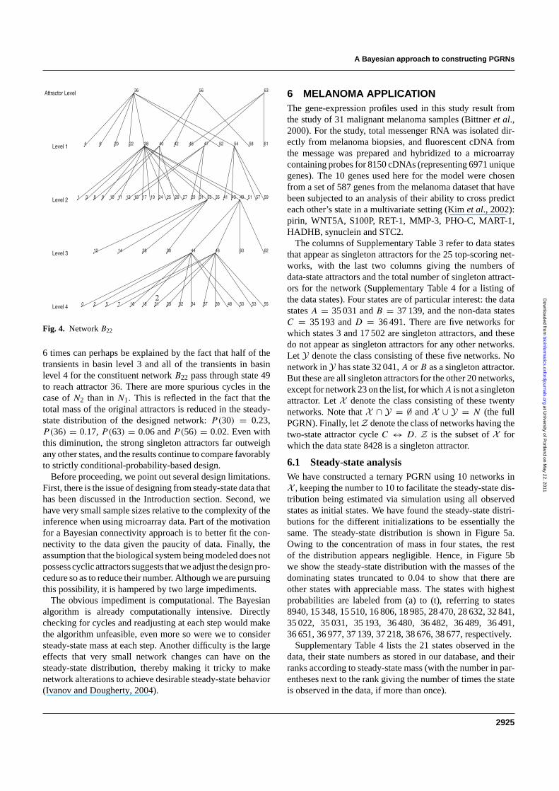
For PBN N2, the attractor-basin structures for B21 andB22 are shown in Figures 3 and 4, respectively. B21 hastwo singleton attractors, states 30 and 56, whereas B22 hasthree singleton attractors, states 36, 56 and 63. The steady-state distribution for N2 has been obtained via simulation.Attractors 30 and 36 carry most of the steady-state mass, withP(30) = 0.51 and P(36) = 0.48. The other attractors, 56and 63, carry negligible mass. A key point is the small basinsof attractors 56 and 63. Supplementary Table 2 shows theattractors, both singleton and cyclic, in the 10 networks takento form the designed PBN. The most important point is thatstates 30 and 36 are singleton attractors in all 10 Boolean net-works. State 63, which occurred once in the sample taken fromthe steady-state distribution, appears in 6 out of the 10, andstate 56, which did not occur in the sample, does not appear.The anomalous appearance of state 49 as a singleton attractor

2924

at University of P

ortland on May 22, 2011

bioinformatics.oxfordjournals.org

Dow

nloaded from

A Bayesian approach to constructing PGRNs

Fig. 4. Network B22

6 times can perhaps be explained by the fact that half of thetransients in basin level 3 and all of the transients in basinlevel 4 for the constituent network B22 pass through state 49to reach attractor 36. There are more spurious cycles in thecase of N2 than in N1. This is reflected in the fact that thetotal mass of the original attractors is reduced in the steady-state distribution of the designed network: P(30) = 0.23,P(36) = 0.17, P(63) = 0.06 and P(56) = 0.02. Even withthis diminution, the strong singleton attractors far outweighany other states, and the results continue to compare favorablyto strictly conditional-probability-based design.

Before proceeding, we point out several design limitations.First, there is the issue of designing from steady-state data thathas been discussed in the Introduction section. Second, wehave very small sample sizes relative to the complexity of theinference when using microarray data. Part of the motivationfor a Bayesian connectivity approach is to better fit the con-nectivity to the data given the paucity of data. Finally, theassumption that the biological system being modeled does notpossess cyclic attractors suggests that we adjust the design pro-cedure so as to reduce their number. Although we are pursuingthis possibility, it is hampered by two large impediments.

The obvious impediment is computational. The Bayesianalgorithm is already computationally intensive. Directlychecking for cycles and readjusting at each step would makethe algorithm unfeasible, even more so were we to considersteady-state mass at each step. Another difficulty is the largeeffects that very small network changes can have on thesteady-state distribution, thereby making it tricky to makenetwork alterations to achieve desirable steady-state behavior(Ivanov and Dougherty, 2004).

6 MELANOMA APPLICATIONThe gene-expression profiles used in this study result fromthe study of 31 malignant melanoma samples (Bittner et al.,2000). For the study, total messenger RNA was isolated dir-ectly from melanoma biopsies, and fluorescent cDNA fromthe message was prepared and hybridized to a microarraycontaining probes for 8150 cDNAs (representing 6971 uniquegenes). The 10 genes used here for the model were chosenfrom a set of 587 genes from the melanoma dataset that havebeen subjected to an analysis of their ability to cross predicteach other’s state in a multivariate setting (Kim et al., 2002):pirin, WNT5A, S100P, RET-1, MMP-3, PHO-C, MART-1,HADHB, synuclein and STC2.

The columns of Supplementary Table 3 refer to data statesthat appear as singleton attractors for the 25 top-scoring net-works, with the last two columns giving the numbers ofdata-state attractors and the total number of singleton attract-ors for the network (Supplementary Table 4 for a listing ofthe data states). Four states are of particular interest: the datastates A = 35 031 and B = 37 139, and the non-data statesC = 35 193 and D = 36 491. There are five networks forwhich states 3 and 17 502 are singleton attractors, and thesedo not appear as singleton attractors for any other networks.Let Y denote the class consisting of these five networks. Nonetwork in Y has state 32 041, A or B as a singleton attractor.But these are all singleton attractors for the other 20 networks,except for network 23 on the list, for which A is not a singletonattractor. Let X denote the class consisting of these twentynetworks. Note that X ∩ Y = ∅ and X ∪ Y = N (the fullPGRN). Finally, let Z denote the class of networks having thetwo-state attractor cycle C ↔ D. Z is the subset of X forwhich the data state 8428 is a singleton attractor.

6.1 Steady-state analysisWe have constructed a ternary PGRN using 10 networks inX , keeping the number to 10 to facilitate the steady-state dis-tribution being estimated via simulation using all observedstates as initial states. We have found the steady-state distri-butions for the different initializations to be essentially thesame. The steady-state distribution is shown in Figure 5a.Owing to the concentration of mass in four states, the restof the distribution appears negligible. Hence, in Figure 5bwe show the steady-state distribution with the masses of thedominating states truncated to 0.04 to show that there areother states with appreciable mass. The states with highestprobabilities are labeled from (a) to (t), referring to states8940, 15 348, 15 510, 16 806, 18 985, 28 470, 28 632, 32 841,35 022, 35 031, 35 193, 36 480, 36 482, 36 489, 36 491,36 651, 36 977, 37 139, 37 218, 38 676, 38 677, respectively.

Supplementary Table 4 lists the 21 states observed in thedata, their state numbers as stored in our database, and theirranks according to steady-state mass (with the number in par-entheses next to the rank giving the number of times the stateis observed in the data, if more than once).

2925

at University of P

ortland on May 22, 2011

bioinformatics.oxfordjournals.org

Dow

nloaded from

X.Zhou et al.

Fig. 5. Estimated distribution after long run: (a) steady-statedistribution; (b) truncation at 0.04.

Considering the total number, 310 = 59 049, of states, forthe most part the data states are fairly high ranked in the steady-state distribution, which is expected. The situation is morestriking if we note that data states A and B carry over half(54%) of the steady-state mass. Almost another quarter ofthe steady-state mass is carried by the non-data states C andD, each carrying 11.3% of the mass. They are very close tostates A and B: state C differs from state A only in PHO-C, with PHO-C having value 1 in C and value 0 in A; andstate D differs from state B only in MMP-3 and PHO-C,with MMP-3 and PHO-C having value 0 in D and value 1in state B. Altogether, the four states A, B, C, and D carryalmost 75% of the steady-state mass and they agree for six ofthe component genes, differing only among the genes RET-1,MMP-3, PHO-C and STC2.

6.2 Connectivity analysisA key interest in constructing PGRNs is to examine the con-nectivity of the constituent networks, since the entire Bayesiandesign is predicated on optimizing connectivity. Moreover,since it is the attractors of the constituent networks that com-prise the PGRN attractors, we would like to investigate therelationship between connectivity and attractors.

A connectivity matrix is associated with each of the 25 net-works (the full set of connectivity matrices being provided onthe companion website). In the matrices, rows refer to tar-gets and columns refer to predictors. For individual networks,most of the time targets have three predictors, but not always.Nine matrices (Supplementary Tables 3–11) provide summaryviews of the connectivity across the 25 constituent networks.

Matrix M1 gives the overall summary. Note that WNT5A isa predictor for five genes in all 25 networks, and a predictorfor a sixth gene in almost all of the networks. Although lessso, pirin and S100P are also frequent predictors. Note alsothat pirin and MMP-3 are always predicted by the same threegenes. Except for a couple of instances, this is also true forsynuclein and STC2. Since the matrix gives collective con-nectivity across the full PGRN, these connectivity relationshold regardless of whether a network is a member of X or Y .

Matrices M2, M3 and M4, summarize the connectivityinformation for classes Y , X and Z , respectively. Note theperfect consistency of predictors for pirin, MP-3, synucleinand STC2. Also note that STC2 is a predictor of WNT5A inonly two of the networks.

Since we want to compare connectivity relations betweenX and Y , we consider the matrix M5 = |M3 − 4M2|, whereall operations are componentwise. The disparity in countsbetween X and Y has been balanced by multiplying M2

by 4. The absolute value is taken because we wish to con-sider the absolute discrepancy. Note that there are very fewlarge discrepancies. The matter is further clarified by formingthe matrix M6 by zeroing out all entries in M5 less than 5.This is done because a random variation of 1 in matrix M2

can create a difference of 4 in M5. The fact that most ofthe entries in matrix M6 are 0 indicates a very strong con-gruency of connectivity between the two classes of networkshaving very different singleton attractors. There are really onlythree differences: WNT5A is predicted frequently by STC2in X but not in Y , and it is predicted somewhat frequently(twice) by MMP-3 in Y but never in X . Analogous commentsapply to PHO-C and MART-1 as targets. The key point here isthat optimizing connectivity has lead to fairly consistent con-nectivity; however, it has produced two classes of networkswith significantly different attractors. This shows that focus-ing on connectivity does not necessarily preclude discoveringa rich attractor structure. We conjecture that this phenomenonis in agreement with real networks because, even in widelyvarying contexts, one would not expect a significant changein connectivity.

2926

at University of P

ortland on May 22, 2011

bioinformatics.oxfordjournals.org

Dow

nloaded from

A Bayesian approach to constructing PGRNs

Turning to the class Z we let matrix M7 = M3 − M4.Recalling that Z ⊂ X , we see that M7 gives the connectivitysummary for the class difference X − Z . To compare Z andX − Z , we define the matrix M8 = |M4 − (3/2)M7|, wherethe factor 3/2 is necessary to correct the difference in classsizes. Matrix M9 is constructed by turning to 0 all entries inM8 less than 3. It is interpreted similarly to M6. Note that it ispractically all 0s. Even the PHO-C change is slight (3.5). Theonly significant change is for RET-1, with pirin and S100Pbeing frequent predictors for class Z but not for class X −Z ,and PHO-C being a frequent predictor for X − Z but not forZ . This means that occurrence of the attractor cycle C ↔ D,which possesses significant steady-state mass, happens withvery little change in connectivity.

7 CONCLUSIONWe have proposed a fully Bayesian approach to construct-ing PGRNs emphasizing network topology. The methodcomputes the possible parent sets of each gene, the corres-ponding predictors, and the associated probabilities basedon a nonlinear perceptron model, using a reversible jumpMCMC technique, and a MCMC method is employed tosearch the network configurations. In proceeding with atopology-based approach, our hypothesis was that construc-tion of transcriptional regulatory networks using a method thatoptimizes connectivity would capture features expected frombiology. This has clearly been the result with regard to theconsidered melanoma study. When operated, the PGRN pro-duces a steady-state distribution containing attractors that areeither identical or very similar to the original observations.Moreover, many of the attractors are singletons, mimick-ing the biological propensity to stably occupy a given state.Most interestingly, the connectivity rules for the most optimalgenerated networks constituting the PGRN are remarkablysimilar, as would be expected for a network operating ona distributed basis, with strong interactions between thecomponents.

ACKNOWLEDGEMENTSThe authors would like to thank the anonymous reviewers fortheir careful reading of manuscript and their constructive com-ments. This research was supported by the National Human

Genome Research Institute and the Translational GenomicsResearch Institute. I.I. was supported by the National CancerInstitute under grant CA90301. X.W. was supported inpart by the US National Science Foundation under grantDMS-0244583.

REFERENCESAndrieu,C., Freitas,J. and Doucet,A. (2001) Robust full Bayesian

learning for neural networks. Neural Comput., 13, 2359–2407.Bittner,M., Meltzer,P., Khan,M., Chen,Y., Jiang,Y., Seftor,E.,

Hendrix,M., Radmacher,M., Simon,R., Yakhini,Z. et al. (2000)Molecular classification of cutaneous malignant melanoma bygene expression profiling. Nature, 406, 536–540.

Friedman,N., Linial,M., Nachman,I. and Pe’er,D. (2000) UsingBaysian network to analyze expression data. Comput. Biol., 7,601–620.

Giudici,D. and Castelo,R. (2003) Improving Markov chain MonteCarlo model search for data mining. Mach. Learning, 50,127–158.

Hartemink,A.J., Gifford,D.K., Jaakkola,T.S. and Young,R.A. (2001)Using graphical models and genomic expression data tostatistically validate models of genetic regulatory networks.Pacific Symp. Biocomput., 6, 23–32.

Ivanov,I. and Dougherty,E.R. (2004) Reduction mappings betweenprobabilistic Boolean networks. Appl. Signal Process., 4,125–131.

Kauffman,S.A. (1993) The Origins of Order: Self-organization andSelection in Evolution. Oxford University Press, NY.

Kim,S., Li,H., Chen,Y., Cao,N., Dougherty,E.R., Bittner,M.L. andSuh,E.B. (2002) Can Markov chain Models mimic biologicalregulation? J. Biol. Sys., 10, 337–357.

Robert,C.P. and Casella,G. (1999) Monte Carlo Statistical Methods.Springer-Verlag, NY.

Shmulevich,I., Dougherty,E.R., Kim,S. and Zhang,W. (2002a) Prob-abilistic Boolean networks: a rule-based uncertainty model forgene regulatory networks. Bioinformatics, 18, 261–274.

Shmulevich,I. Dougherty,E.R. and Zhang,W. (2002b) Gene per-turbation and intervention in probabilistic Boolean networksbioinformatics. Bioinformatics, 18, 1319–1331.

Shmulevich,I., Dougherty,E.R. and Zhang,W. (2002c) From Booleanto probabilistic Boolean networks as models of genetic regulatorynetworks. Proc. IEEE, 90, 1778–1792.

Zhou,X., Wang,X. and Dougherty,E.R. (2003) Construction ofgenomic networks using mutual-information clustering andreversible-jump Markov-chain-Monte-Carlo predictor design.Signal Processing, 84, 745–761.

2927

at University of P

ortland on May 22, 2011

bioinformatics.oxfordjournals.org

Dow

nloaded from