RD

JM

a

©

GEOPHYSICS, VOL. 73, NO. 5 �SEPTEMBER-OCTOBER 2008�; P. VE235–VE241, 15 FIGS.10.1190/1.2957947

esolving near-seabed velocity anomalies:eep water offshore eastern India

uergen Fruehn1, Ian F. Jones1, Victoria Valler1, Pranaya Sangvai2, Ajoy Biswal2, andohit Mathur2

vmdlmma

�upTnmsao

hddrpscfi

pmetasei

receiveiongeo

com;A

ABSTRACT

Imaging in deep-water environments poses a specific set ofchallenges, both in data preconditioning and velocity modelbuilding. These challenges include scattered, complex 3Dmultiples, aliased noise, and low-velocity shallow anomaliesassociated with channel fills and gas hydrates. We describe anapproach to tackling such problems for data from deep wateroff the east coast of India, concentrating our attention on iter-ative velocity model building, and more specifically the reso-lution of near-surface and other velocity anomalies. In the re-gion under investigation, the velocity field is complicated bynarrow buried canyons �500 m wide� filled with low-velocitysediments, which give rise to severe pull-down effects; possi-ble free-gas accumulation below an extensive gas-hydratecap, causing dimming of the image below �perhaps as a resultof absorption�; and thin-channel bodies with low-velocityfill. Hybrid gridded tomography using a conjugate gradientsolver �with 20-m vertical cell size� was applied to resolvesmall-scale velocity anomalies �with thicknesses of about50 m�. Manual picking of narrow-channel features was usedto define bodies too small for the tomography to resolve.Prestack depth migration, using a velocity model built with acombination of these techniques, could resolve pull-downand other image distortion effects in the final image. The re-sulting velocity field shows high-resolution detail useful inidentifying anomalous geobodies of potential explorationinterest.

INTRODUCTION

Off the east coast of India, the transition from the shallower coast-l waters to the deep shelf often involves significant topographical

Manuscript received by the Editor 23 November 2007; revised manuscript1ION GX Technology, Egham, United Kingdom. E-mail: Juergen.Fruehn@2Reliance Industries Ltd., Mumbai, India. E-mail: Pranaya.Sangvai@RIL.2008 Society of Exploration Geophysicists.All rights reserved.

VE235

ariation in the seabed, which gives rise to numerous effects thatust be dealt with by the processing geophysicist. In addition to

eep channels and steep slopes, we encounter buried channels withow-velocity fills and gas hydrates. Diffracted and “out-of-plane”

ultiples are the norm in these environments �Stewart, 2004� andust be dealt with to derive a reliable velocity model so as to deliver

n acceptable structural image �Stewart et al., 2007�.With the advent of 3D surface-related multiple elimination

SRME�, a theoretically robust approach to complex multiple atten-ation became available; and application of 3D SRME to these dataroves to be very effective �Sangvai et al., 2008; Smith et al., 2008�.he SRME technique, which the Delft University consortium pio-eered �Verschuur et al., 1992�, involves generating a model of theultiples from input data without prior knowledge of the velocity

tructure of the subsurface. Consequently, it is an ideal approach toccompany complex imaging problems when an a priori knowledgef the velocities cannot be assumed.

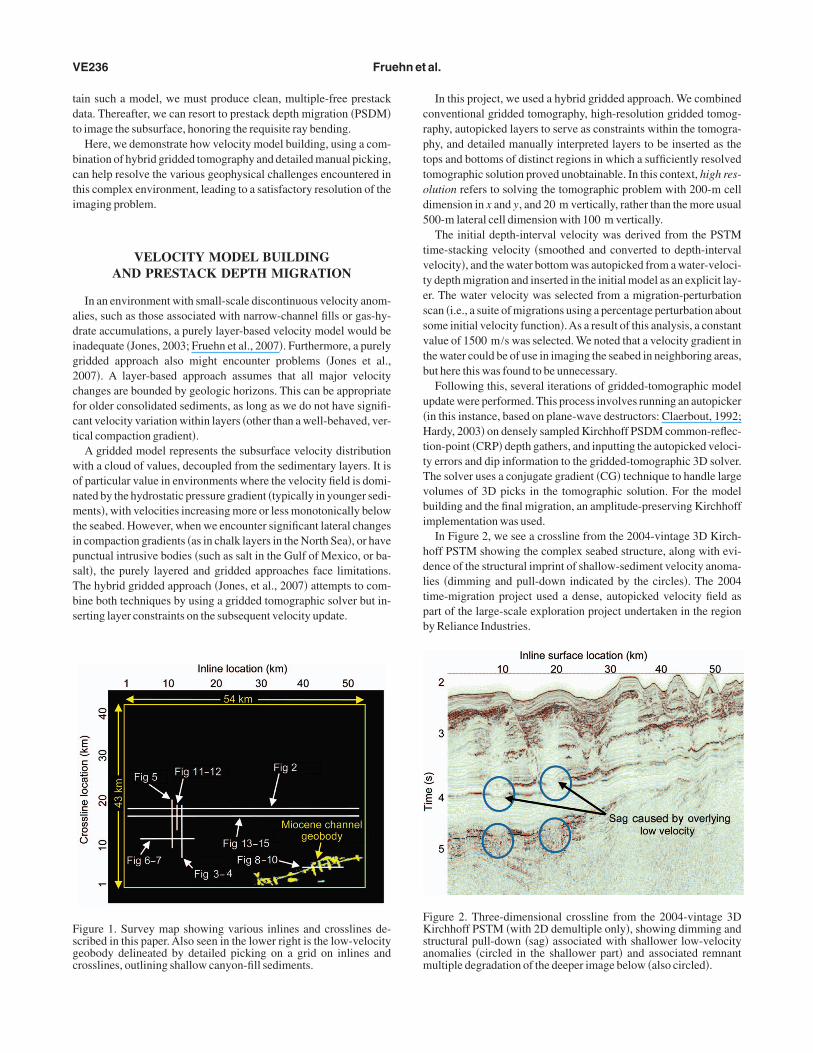
In the data considered here, the water depths range from a fewundred meters to more than 1 km; and for the most part they areeeper than 1.5 km, with deeply incised seabed channels runningown the continental slope. The region under consideration isoughly 43 km by 54 km �some 2200 sq. km�, covering a large ex-loration area of unknown hydrocarbon potential. Figure 1 shows aurvey outline, indicating the locations of various inlines androsslines that are discussed here. In addition, the lower left of thegure shows a canyon-fill geobody, which will be described later.The data were collected in 2004 and imaged after 2D demultiple

rocessing using 3D prestack time migration �PSTM�. This time-do-ain imaging produced very good results overall, but it was consid-

red suboptimal for specific parts of the region. The areas for whichime migration constitutes an inadequate imaging solution are thosereas affected by significant ray bending, such as directly belowteep-sided seafloor canyons or beneath low-velocity geobody lens-s. As with any complex or subtle imaging problem, the key to goodmaging is the derivation of a representative velocity model. To ob-

d 13 February 2008; published online 1 October 2008..com; Ian.Jones@iongeo.com; Victoria.Valler@iongeo.com.

joy.Biswal@RIL.com; Mohit.Mathur@RIL.com.

tdt

bcti

adig2cfct

wonmtipsTbs

crpttod5

tvtessvtb

u�HttTvbi

hdltpb

Fsgc

FKsam

VE236 Fruehn et al.

ain such a model, we must produce clean, multiple-free prestackata. Thereafter, we can resort to prestack depth migration �PSDM�o image the subsurface, honoring the requisite ray bending.

Here, we demonstrate how velocity model building, using a com-ination of hybrid gridded tomography and detailed manual picking,an help resolve the various geophysical challenges encountered inhis complex environment, leading to a satisfactory resolution of themaging problem.

VELOCITY MODEL BUILDINGAND PRESTACK DEPTH MIGRATION

In an environment with small-scale discontinuous velocity anom-lies, such as those associated with narrow-channel fills or gas-hy-rate accumulations, a purely layer-based velocity model would benadequate �Jones, 2003; Fruehn et al., 2007�. Furthermore, a purelyridded approach also might encounter problems �Jones et al.,007�. A layer-based approach assumes that all major velocityhanges are bounded by geologic horizons. This can be appropriateor older consolidated sediments, as long as we do not have signifi-ant velocity variation within layers �other than a well-behaved, ver-ical compaction gradient�.

A gridded model represents the subsurface velocity distributionith a cloud of values, decoupled from the sedimentary layers. It isf particular value in environments where the velocity field is domi-ated by the hydrostatic pressure gradient �typically in younger sedi-ents�, with velocities increasing more or less monotonically below

he seabed. However, when we encounter significant lateral changesn compaction gradients �as in chalk layers in the North Sea�, or haveunctual intrusive bodies �such as salt in the Gulf of Mexico, or ba-alt�, the purely layered and gridded approaches face limitations.he hybrid gridded approach �Jones, et al., 2007� attempts to com-ine both techniques by using a gridded tomographic solver but in-erting layer constraints on the subsequent velocity update.

igure 1. Survey map showing various inlines and crosslines de-cribed in this paper. Also seen in the lower right is the low-velocityeobody delineated by detailed picking on a grid on inlines androsslines, outlining shallow canyon-fill sediments.

In this project, we used a hybrid gridded approach. We combinedonventional gridded tomography, high-resolution gridded tomog-aphy, autopicked layers to serve as constraints within the tomogra-hy, and detailed manually interpreted layers to be inserted as theops and bottoms of distinct regions in which a sufficiently resolvedomographic solution proved unobtainable. In this context, high res-lution refers to solving the tomographic problem with 200-m cellimension in x and y, and 20 m vertically, rather than the more usual00-m lateral cell dimension with 100 m vertically.

The initial depth-interval velocity was derived from the PSTMime-stacking velocity �smoothed and converted to depth-intervalelocity�, and the water bottom was autopicked from a water-veloci-y depth migration and inserted in the initial model as an explicit lay-r. The water velocity was selected from a migration-perturbationcan �i.e., a suite of migrations using a percentage perturbation aboutome initial velocity function�.As a result of this analysis, a constantalue of 1500 m/s was selected. We noted that a velocity gradient inhe water could be of use in imaging the seabed in neighboring areas,ut here this was found to be unnecessary.

Following this, several iterations of gridded-tomographic modelpdate were performed. This process involves running an autopickerin this instance, based on plane-wave destructors: Claerbout, 1992;ardy, 2003� on densely sampled Kirchhoff PSDM common-reflec-

ion-point �CRP� depth gathers, and inputting the autopicked veloci-y errors and dip information to the gridded-tomographic 3D solver.he solver uses a conjugate gradient �CG� technique to handle largeolumes of 3D picks in the tomographic solution. For the modeluilding and the final migration, an amplitude-preserving Kirchhoffmplementation was used.

In Figure 2, we see a crossline from the 2004-vintage 3D Kirch-off PSTM showing the complex seabed structure, along with evi-ence of the structural imprint of shallow-sediment velocity anoma-ies �dimming and pull-down indicated by the circles�. The 2004ime-migration project used a dense, autopicked velocity field asart of the large-scale exploration project undertaken in the regiony Reliance Industries.

igure 2. Three-dimensional crossline from the 2004-vintage 3Dirchhoff PSTM �with 2D demultiple only�, showing dimming and

tructural pull-down �sag� associated with shallower low-velocitynomalies �circled in the shallower part� and associated remnantultiple degradation of the deeper image below �also circled�.

sblninve

tccvmanpt

Ppepi

mawtdts

ta

G

gpadftll

cr2ttattpst

rsabfel

FDr

FStss1

Near-seabed velocity anomalies VE237

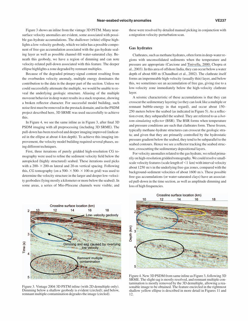
Figure 3 shows an inline from the vintage 3D PSTM. Many near-urface velocity anomalies are evident, some associated with possi-le gas-hydrate accumulations. The shallower �white� ellipse high-ights a low-velocity geobody, which we infer has a possible compo-ent of free-gas accumulation associated with the gas-hydrate seal-ng layer as well as possible channel-fill water-saturated clay. Be-eath this geobody, we have a region of dimming and can noteelocity-related pull-down associated with this feature. The deeperllipse highlights a zone degraded by remnant multiples.

Because of the degraded primary-signal content resulting fromhe overburden velocity anomaly, multiple energy dominates theontribution to the data in the deeper part of the section. Unless weould successfully attenuate the multiple, we would be unable to re-eal the underlying geologic structure. Aliasing of the multipleoveout behavior in deep water results in a stack response, showingbroken reflector character. For successful model building, such

oise first must be removed in the prestack domain; and in the PSDMroject described here, 3D SRME was used successfully to achievehis.

In Figure 4, we see the same inline as in Figure 3, after final 3DSDM imaging with all preprocessing �including 3D SRME�. Theull-down has been resolved and deeper imaging improved �indicat-d in the ellipse at about 4-km depth�. To achieve this imaging im-rovement, the velocity model building required several phases, us-ng different techniques.

First, three iterations of purely gridded high-resolution CG to-ography were used to refine the sediment velocity field below the

utopicked �highly structured� seabed. These iterations used picksith a 200- � 200-m lateral and 20-m vertical spacing. Following

his, CG tomography �on a 500- � 500- � 100-m grid� was used toetermine the velocity structure in the larger and deeper low-veloci-y geobodies �lying mostly a kilometer or more below the seabed�. Inome areas, a series of Mio-Pliocene channels were visible; and

igure 3. Vintage 2004 3D PSTM inline �with 2D demultiple only�.imming below a shallow geobody is evident �circled�; and below,

emnant multiple contamination degrades the image �circled�.

hese were resolved by detailed manual picking in conjunction withmigration velocity-perturbation scan.

as hydrates

Clathrates, such as methane hydrates, often form in deep-water re-ions with unconsolidated sediments when the temperature andressure are appropriate �Carcione and Tinivella, 2000; Chopra etl., 2003�. In this area of offshore India, they can occur below a waterepth of about 600 m �Chaudhuri et al., 2002�. The clathrate itselforms an impermeable high-velocity �usually thin� layer, and belowhis, we sometimes see an accumulation of free gas, giving rise to aow-velocity zone immediately below the high-velocity clathrateayer.

A seismic characteristic of these accumulations is that they canrosscut the sedimentary layering �so they can look like a multiple oremnant bubble-energy in that regard�, and occur about 150–50 meters below the seabed �as indicated in Figure 5�. As a reflec-ion event, they subparallel the seabed. They are referred to as a bot-om-simulating reflector �BSR�. The BSR forms when temperaturend pressure conditions are such that clathrates form. These frozen,ypically methane-hydrate structures can crosscut the geologic stra-a; and given that they are primarily controlled by the hydrostaticressure gradient below the seabed, they tend to be subparallel to theeabed contours. Hence we see a reflector tracking the seabed struc-ure, crosscutting the sedimentary depositional layers.

For velocity anomalies related to the gas hydrate, we relied prima-ily on high-resolution gridded tomography. We could resolve small-cale velocity features �scale length of �1 km� with interval velocitybout 1250 m/s in the underlying free-gas zones, compared with theackground-sediment velocities of about 1600 m/s. These possibleree-gas accumulations �or water-saturated clays� have an associat-d pull-down in the time section, as well as amplitude dimming andoss of high frequencies.

igure 4. New 3D PSDM from same inline as Figure 3, following 3DRME. The slight sag is mostly resolved, and remnant multiple con-

amination is mostly removed by the 3D demultiple, allowing a rea-onable image to be obtained. The feature encircled in the rightmosthallow yellow ellipse is described in more detail in Figures 11 and2.

tws

Bida

pTfilmebtm

vacdrbt

C

jawspp

FttufOgPtfTc

Fefl

Fimd

VE238 Fruehn et al.

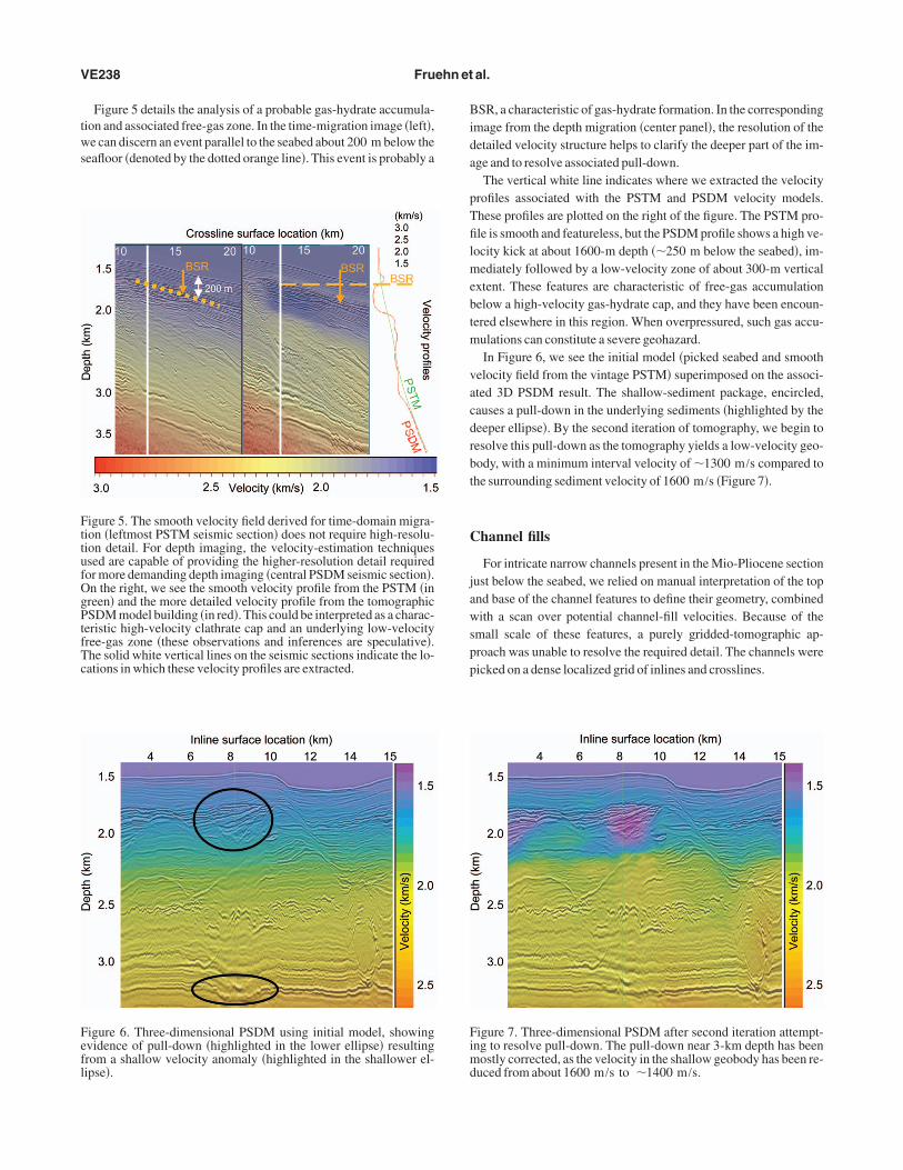
Figure 5 details the analysis of a probable gas-hydrate accumula-ion and associated free-gas zone. In the time-migration image �left�,e can discern an event parallel to the seabed about 200 m below the

eafloor �denoted by the dotted orange line�. This event is probably a

igure 5. The smooth velocity field derived for time-domain migra-ion �leftmost PSTM seismic section� does not require high-resolu-ion detail. For depth imaging, the velocity-estimation techniquessed are capable of providing the higher-resolution detail requiredor more demanding depth imaging �central PSDM seismic section�.n the right, we see the smooth velocity profile from the PSTM �inreen� and the more detailed velocity profile from the tomographicSDM model building �in red�. This could be interpreted as a charac-

eristic high-velocity clathrate cap and an underlying low-velocityree-gas zone �these observations and inferences are speculative�.he solid white vertical lines on the seismic sections indicate the lo-ations in which these velocity profiles are extracted.

igure 6. Three-dimensional PSDM using initial model, showingvidence of pull-down �highlighted in the lower ellipse� resultingrom a shallow velocity anomaly �highlighted in the shallower el-ipse�.

SR, a characteristic of gas-hydrate formation. In the correspondingmage from the depth migration �center panel�, the resolution of theetailed velocity structure helps to clarify the deeper part of the im-ge and to resolve associated pull-down.

The vertical white line indicates where we extracted the velocityrofiles associated with the PSTM and PSDM velocity models.hese profiles are plotted on the right of the figure. The PSTM pro-le is smooth and featureless, but the PSDM profile shows a high ve-

ocity kick at about 1600-m depth ��250 m below the seabed�, im-ediately followed by a low-velocity zone of about 300-m vertical

xtent. These features are characteristic of free-gas accumulationelow a high-velocity gas-hydrate cap, and they have been encoun-ered elsewhere in this region. When overpressured, such gas accu-

ulations can constitute a severe geohazard.In Figure 6, we see the initial model �picked seabed and smooth

elocity field from the vintage PSTM� superimposed on the associ-ted 3D PSDM result. The shallow-sediment package, encircled,auses a pull-down in the underlying sediments �highlighted by theeeper ellipse�. By the second iteration of tomography, we begin toesolve this pull-down as the tomography yields a low-velocity geo-ody, with a minimum interval velocity of �1300 m/s compared tohe surrounding sediment velocity of 1600 m/s �Figure 7�.

hannel fills

For intricate narrow channels present in the Mio-Pliocene sectionust below the seabed, we relied on manual interpretation of the topnd base of the channel features to define their geometry, combinedith a scan over potential channel-fill velocities. Because of the

mall scale of these features, a purely gridded-tomographic ap-roach was unable to resolve the required detail. The channels wereicked on a dense localized grid of inlines and crosslines.

igure 7. Three-dimensional PSDM after second iteration attempt-ng to resolve pull-down. The pull-down near 3-km depth has been

ostly corrected, as the velocity in the shallow geobody has been re-uced from about 1600 m/s to �1400 m/s.

wcptw3Tbtud1

wcndcr

U

tcwlwp

wtsnufo

t

Flmip

Fgfi

Fva

Near-seabed velocity anomalies VE239

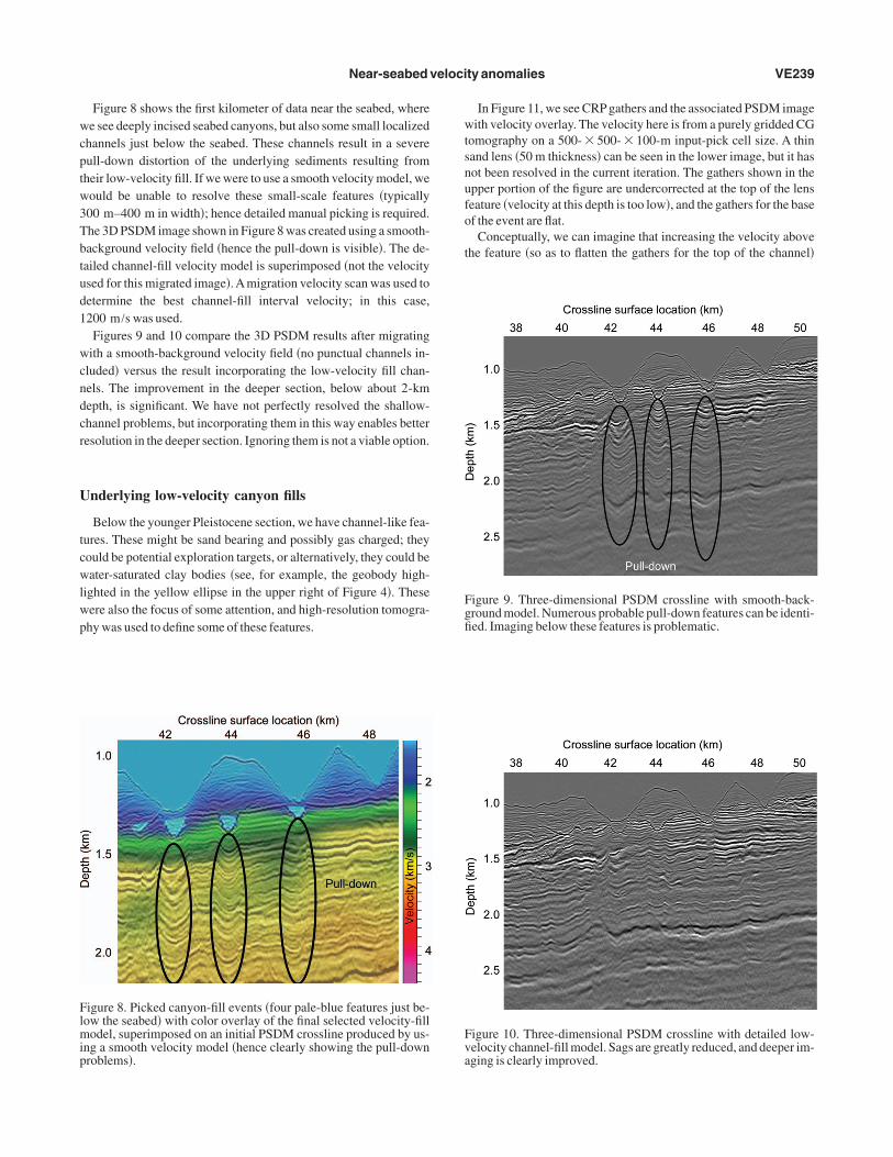
Figure 8 shows the first kilometer of data near the seabed, wheree see deeply incised seabed canyons, but also some small localized

hannels just below the seabed. These channels result in a severeull-down distortion of the underlying sediments resulting fromheir low-velocity fill. If we were to use a smooth velocity model, weould be unable to resolve these small-scale features �typically00 m–400 m in width�; hence detailed manual picking is required.he 3D PSDM image shown in Figure 8 was created using a smooth-ackground velocity field �hence the pull-down is visible�. The de-ailed channel-fill velocity model is superimposed �not the velocitysed for this migrated image�.Amigration velocity scan was used toetermine the best channel-fill interval velocity; in this case,200 m/s was used.

Figures 9 and 10 compare the 3D PSDM results after migratingith a smooth-background velocity field �no punctual channels in-

luded� versus the result incorporating the low-velocity fill chan-els. The improvement in the deeper section, below about 2-kmepth, is significant. We have not perfectly resolved the shallow-hannel problems, but incorporating them in this way enables betteresolution in the deeper section. Ignoring them is not a viable option.

nderlying low-velocity canyon fills

Below the younger Pleistocene section, we have channel-like fea-ures. These might be sand bearing and possibly gas charged; theyould be potential exploration targets, or alternatively, they could beater-saturated clay bodies �see, for example, the geobody high-

ighted in the yellow ellipse in the upper right of Figure 4�. Theseere also the focus of some attention, and high-resolution tomogra-hy was used to define some of these features.

igure 8. Picked canyon-fill events �four pale-blue features just be-ow the seabed� with color overlay of the final selected velocity-fill

odel, superimposed on an initial PSDM crossline produced by us-ng a smooth velocity model �hence clearly showing the pull-downroblems�.

In Figure 11, we see CRP gathers and the associated PSDM imageith velocity overlay. The velocity here is from a purely gridded CG

omography on a 500- � 500- � 100-m input-pick cell size. A thinand lens �50 m thickness� can be seen in the lower image, but it hasot been resolved in the current iteration. The gathers shown in thepper portion of the figure are undercorrected at the top of the lenseature �velocity at this depth is too low�, and the gathers for the basef the event are flat.

Conceptually, we can imagine that increasing the velocity abovehe feature �so as to flatten the gathers for the top of the channel�

igure 9. Three-dimensional PSDM crossline with smooth-back-round model. Numerous probable pull-down features can be identi-ed. Imaging below these features is problematic.

igure 10. Three-dimensional PSDM crossline with detailed low-elocity channel-fill model. Sags are greatly reduced, and deeper im-ging is clearly improved.

wal�

r2t

M

oawoptcpn

epmmw

pseincls

Fguwtot

Ftbstvs

Fcdss

VE240 Fruehn et al.

ould cause the base-channel gathers to curl down �too fast�; so welso need to reduce the channel-fill velocity while increasing the ve-ocity above the channel. This was accomplished in the next iterationas shown in Figure 12�, where the lateral dimensions of the tomog-

igure 11. Top: CRP gathers after the fourth run of PSDM �theseathers are used as input to the next iteration of tomographic-modelpdate�. We can see some residual velocity error �gathers curling up-ard indicates the velocity is still too low� above the channel. Bot-

om: Image associated with these gathers with interval-velocity col-r overlay. The thin-lens feature �encircled� is seen in a larger con-ext in the upper right of Figure 4.

igure 12. Top: CRP gathers after the subsequent update of 3D CGomography. Some of the undercorrection above the channel haseen resolved and the channel velocity itself lowered, so as to pre-erve flat gathers at the channel base. Bottom: Image associated withhese gathers with interval-velocity color overlay, showing the lowelocity in the thin-channel feature. The thin feature �encircled� iseen in a larger context in the upper right of Figure 4.

aphic cell were reduced to 200 m and the vertical dimension to0 m. We consider this to be close to the vertical resolution of ourechnique.

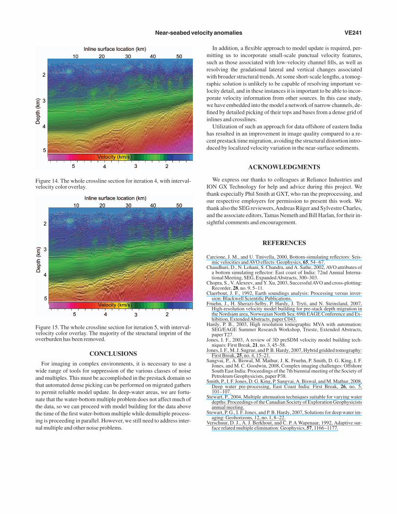
odel evolution

In the following figures, showing a long crossline adjacent to thatf Figure 2, we summarize the evolution of the model. Figure 13 �topnd bottom� compares the first and second iterations, which dealtith only the shallow section, while Figures 14 and 15 compare theverall section. By the fifth iteration, the deep section has been im-roved considerably. During the model building of the shallow sec-ion, the data preprocessing was ongoing so as to apply lengthy pro-esses such as 3D SRME and the other denoise steps. These fullyreprocessed data then were used for deeper model update and the fi-al imaging.

As a consequence, the data input to the earlier model-building it-rations did not have the full denoise preprocessing sequence ap-lied. This is reasonable for deep-water environments, as we haveuch work to do in model building before encountering the firstultiple. Overlapping the preprocessing and model building in thisay also facilitates reduction of overall turnaround time.It is important to note that, for a global tomographic solution, all

arts of the model can be adjusted at each iteration. Hence we can seeubtle changes in the shallow section for some parts of the model,ven at the latter iterations. Once we have imposed a layer constraintn the hybrid scheme �such as for the seabed or detailed picked chan-els�, those parts of the model remain invariant. The update schemeeases to be a truly global one and thus can be viewed as a class ofayer stripping �although we have much more flexibility in a griddedcheme than in a purely layer-based scheme�.

igure 13. Upper panel: First iteration of model update for PSDMrossline down to 3 km. Lower panel: Second iteration of model up-ate down to 3 km. For the most part, the structural imprint of theeabed and underlying sediments has been removed. Both imageshown with interval-velocity color overlay.

wattnttin

msrwrlpwfii

hcd

Itotas

C

C

C

C

F

H

J

J

S

S

S

S

V

Fv

Fvo

Near-seabed velocity anomalies VE241

CONCLUSIONS

For imaging in complex environments, it is necessary to use aide range of tools for suppression of the various classes of noise

nd multiples. This must be accomplished in the prestack domain sohat automated dense picking can be performed on migrated gatherso permit reliable model update. In deep-water areas, we are fortu-ate that the water-bottom multiple problem does not affect much ofhe data, so we can proceed with model building for the data abovehe time of the first water-bottom multiple while demultiple process-ng is proceeding in parallel. However, we still need to address inter-

igure 14. The whole crossline section for iteration 4, with interval-elocity color overlay.

igure 15. The whole crossline section for iteration 5, with interval-elocity color overlay. The majority of the structural imprint of theverburden has been removed.

al multiple and other noise problems.

In addition, a flexible approach to model update is required, per-itting us to incorporate small-scale punctual velocity features,

uch as those associated with low-velocity channel fills, as well asesolving the gradational lateral and vertical changes associatedith broader structural trends.At some short-scale lengths, a tomog-

aphic solution is unlikely to be capable of resolving important ve-ocity detail, and in these instances it is important to be able to incor-orate velocity information from other sources. In this case study,e have embedded into the model a network of narrow channels, de-ned by detailed picking of their tops and bases from a dense grid of

nlines and crosslines.Utilization of such an approach for data offshore of eastern India

as resulted in an improvement in image quality compared to a re-ent prestack time migration, avoiding the structural distortion intro-uced by localized velocity variation in the near-surface sediments.

ACKNOWLEDGMENTS

We express our thanks to colleagues at Reliance Industries andON GX Technology for help and advice during this project. Wehank especially Phil Smith at GXT, who ran the preprocessing, andur respective employers for permission to present this work. Wehank also the SEG reviewers,Andreas Rüger and Sylvestre Charles,nd the associate editors, Tamas Nemeth and Bill Harlan, for their in-ightful comments and encouragement.

REFERENCES

arcione, J. M., and U. Tinivella, 2000, Bottom-simulating reflectors: Seis-mic velocities andAVO effects: Geophysics, 65, 54–67.

haudhuri, D., N. Lohani, S. Chandra, and A. Sathe, 2002, AVO attributes ofa bottom simulating reflector: East coast of India: 72nd Annual Interna-tional Meeting, SEG, ExpandedAbstracts, 300–303.

hopra, S., V. Alexeev, and Y. Xu, 2003, SuccessfulAVO and cross-plotting:Recorder, 28, no. 9, 5–11.

laerbout, J. F., 1992, Earth soundings analysis: Processing versus inver-sion: Blackwell Scientific Publications.

ruehn, J., H. Sherazi-Selby, P. Hardy, J. Tryti, and N. Steinsland, 2007,High-resolution velocity model building for pre-stack depth migration inthe Nordsjøn area, Norwegian North Sea: 69th EAGE Conference and Ex-hibition, ExtendedAbstracts, paper C043.

ardy, P. B., 2003, High resolution tomographic MVA with automation:SEG/EAGE Summer Research Workshop, Trieste, Extended Abstracts,paper T27.

ones, I. F., 2003, A review of 3D preSDM velocity model building tech-niques: First Break, 21, no. 3, 45–58.

ones, I. F., M. J. Sugrue, and P. B. Hardy, 2007, Hybrid gridded tomography:First Break, 25, no. 4, 15–21.

angvai, P., A. Biswal, M. Mathur, J. K. Fruehn, P. Smith, D. G. King, I. F.Jones, and M. C. Goodwin, 2008, Complex imaging challenges: OffshoreSouth East India: Proceedings of the 7th biennial meeting of the Society ofPetroleum Geophysicists, paper P38.

mith, P., I. F. Jones, D. G. King, P. Sangvai, A. Biswal, and M. Mathur, 2008,Deep water pre-processing, East Coast India: First Break, 26, no. 5,101–107.

tewart, P., 2004, Multiple attenuation techniques suitable for varying waterdepths: Proceedings of the Canadian Society of Exploration Geophysicistsannual meeting.

tewart, P. G., I. F. Jones, and P. B. Hardy, 2007, Solutions for deep water im-aging: Geohorizons, 12, no. 1, 8–22.

erschuur, D. J., A. J. Berkhout, and C. P. A Wapenaar, 1992, Adaptive sur-face related multiple elimination: Geophysics, 57, 1166–1177.