RESOLVING DISCREPANCIES IN PREDICTING CRITICAL

RATES IN LOW PRESSURE STRIPPER

GAS WELLS

by

OLUFEMI AWOLUSI, B.Sc.

A THESIS

IN

PETROLEUM ENGINEERING

Submitted to the Graduate Faculty of Texas Tech University in

Partial Fulfillment of the Requirements for

the Degree of

MASTER OF SCIENCE

IN

PETROLEUM ENGINEERING

Approved

Teddy Oetama Chairperson of the Committee

James F. Lea

Accepted

John Borrelli Dean of the Graduate School

August, 2005

ACKNOWLEDGEMENTS

I am particularly grateful to everyone that has contributed to the success of this

thesis and the accomplishment of my Master of Science program. I wish to thank Dr.

Teddy Oetama and Dr. James F. Lea for their support, listening ear and guidance through

the course of this project. I couldn’t do without the help of Joe McInerney in setting up

the laboratory apparatus and process required for the experiment. I also want to

appreciate the help of Drs. H. Winkler, L. Heinze, A.S. Lawal and P. Adisoemarta during

the course of the project.

Of course, I very much appreciate the moral and spiritual support of my parents:

David and Abigail Awolusi, my siblings, my uncle: Mr. Jacob Odina and his family, my

aunt: Mrs. E. Alao and her family, Simisola, all the guys over at the petroleum

engineering department of Texas Tech University and Christ Community Church. Above

all, I thank the Good Lord for his grace upon my life and making my dreams come true.

ii

TABLE OF CONTENTS

ACKNOWLEDGEMENTS ………………..……………………………………………. ii

ABSTRACT …………………………………..……...…………………………............. vi

LIST OF FIGURES ………………………………….....………….……….………….. vii

LIST OF SYMBOLS …………………...……………..………………..…….………… ix

CHAPTER

I INTRODUCTION ………………………………..………………..…….... 1

1.1 Background Information ……………………………..…….…………. 1

1.2 Statement of Problem ...………………..…………………..………...... 4

1.3 Scope and Limitations of Study ………………………...…..…..…….. 4

II LITERATURE REVIEW …………………………...……………..……..... 6

2.1 Symptoms of Liquid Loading ………………………..…...……......…. 6

2.1.1 Erratic Flow Pattern Indicated on Gas Chart ………..….….... 6

2.1.2 Sharp Drop in Decline Curve ……………...……..…...……... 7

2.1.3 Increase in Tubing – Casing Pressure Difference ………........ 8

2.1.4 Higher Pressure Gradient ……………………..…….....…….. 9

2.2 Critical Velocity Models Based on Spherical Droplet ……………..... 10

2.2.1 Critical Velocity Definition …………...…………....…..…... 11

iii

2.2.2 Droplet Size …………………………………..…..…...……. 12

2.2.3 Wellbore Liquids ……………………..……….…….…...…. 12

2.2.4 Flow Pattern Recognition ………………..………..…..……. 14

2.3 Critical Velocity Model Based on Flat-Shaped Droplet ..………..…... 17

2.4 Critical Velocity Model Based on Flow Conditions ……………........ 18

2.5 Critical Velocity Model Based on a Turner Ratio ……….…...……… 19

2.6 Factors Affecting Minimum Flowrate for Liquid Removal …….….... 22

III METHODOLOGY. ………………………………………………………. 25

3.1 Equipment Used ………………………………………..………..…... 25

3.2 Data Collection Procedure ……………………..………...………….. 27

3.3 Gas Flow Through Choke ……………………..............…………...... 28

IV DISCUSSION OF RESULTS ……………………...……...……………... 30

4.1 Flow Regime and Mapping ………………..………………..……….. 31

4.2 Comparison of Critical Rate Predictions ……………………….…… 32

4.3 Test Model Development ……………..……………………...……… 35

4.4 The Liquid-Gas-Ratio (LGR) Effect ………………..……………….. 39

V CONCLUSIONS AND RECOMMENDATIONS …………..…..…...…... 40

5.1 Conclusions …………………………………………………...……... 40

5.2 Recommendations ……….....................................………….….……. 41

iv

REFERENCES ………………………………………………...………...……..……… 42

APPENDICES ……………………………………………………...……...…………... 44

A MEASURED CRITICAL FLOW RATE DATA ……………….…............ 44

B TURNER’S AND COLEMAN’S CRITICAL VELOCITY

EQUATIONS …………………………………………………………...... 50

C LI’S CRITICAL VELOCITY EQUATIONS …………………..……...…. 54

D NOSSEIR’S CRITICAL VELOCITY EQUATIONS ……..……..………. 58

v

ABSTRACT

The minimum gas rate for unloading liquids from a gas well has been the

subject of much interest, especially in old gas producing fields with declining reservoir

pressures. For low-pressure stripper gas wells, liquid production accumulating in the

tubing is a pivotal factor that could lead to premature well abandonment and a huge

detrimental difference in the economic viability of the well.

Some notable correlations that exist for predicting the critical rate required for

liquid unloading in gas wells include Turner et al., (1969), Coleman et al., (1991),

Nosseir et al. (1997), Li et al. (2001) and Veeken et al., (2003). However, these

correlations offer divergent views on the critical rates needed for liquid unloading, and

for some correlations in particular, at low wellhead pressures below 50 psia.

The objectives of this research are to evaluate discrepancies in the previous

work on critical gas velocities required to keep liquid from accumulating in the tubing.

Also during the course of the work, data were collected using a flow test facility at Texas

Tech University. The critical gas rates were experimentally measured in order to

determine an improved correlation with specific application for low-pressure stripper gas

wells below 50 psia and at average temperature of 64 oF.

vi

LIST OF FIGURES

1.1 A Typical Gas Well Decline Curve ……...…..………...……..…………….…... 2

1.2 Gas Well Liquid Loading Process …..………………..……...………..………... 2

2.1 Gas Chart Indicating Liquid Loading …………………...…………....…….….. 7

2.2 Decline Curve Profile with Actual Loading …………………..……………...… 8

2.3 The Casing – Tubing Pressure Profile of a Loading Well .….……..…….…..…. 9

2.4 Pressure Gradient of a Liquid Loading Well .……………….……….....………. 9

2.5 Rate of Water Condensation for an 8,000-ft Well ……………....…….…….… 13

2.6 Flow Patterns in Vertical Two-Phase Flow ………………..…………......….... 14

2.7 Flow Pattern Mapping with Transitions ………………………..……..……..... 15

2.8 Flow Regime Map of Duns and Ros ………...…………….....…….….….…... 16

2.9 Deformation of a Free-Falling Droplet …….……………………...…….....…. 17

2.10 Turner Ratio vs. Product of ‘A’ and Wellhead Pressure ………………...…...... 20

2.11 Comparison of Turner’s, Coleman’s and Veeken’s Predictions ….......…....….. 21

2.12 Temperature Effect on Minimum Gas Flowrate ….……...…………………… 22

2.13 Flow Diameter Effect on Minimum Gas Flowrate …………..………...……... 23

2.14 Gas Gravity Effect on Minimum Gas Flowrate ….…………...…….....……… 24

3.1 Schematic Diagram of Test Facility ………………..…….…………....……… 26

vii

3.2 MC 10 Flow Curves …………………………………….…….…..……..……. 29

4.1 Line of Best Fit for Measured Data ……………………………..……...….…. 31

4.2 Flow Pattern Map of Test data ………………………………….…………….. 32

4.3 Critical Rate Comparisons …………………………………………….......….. 33

4.4 Coleman’s Data for Pressures Below 110 psia .………………...…...……...… 34

4.5 Drag Coefficients for Spheres, Disks and Cylinders ……………….………… 37

4.6 Critical Rate and Critical Velocity Relationship ………………………..…….. 38

4.7 Critical Rate vs. LGR for Developed Model…………………..…….....……... 39

viii

LIST OF SYMBOLS

Symbols Definition

At Area of Tubing ID (ft2)

A Inflow performance parameter

At Tubing area (ft2)

Ad Droplet area (ft2)

Cd Drag coefficient

Cv Coefficient of flow

d Droplet diameter (ft)

FG Downward gravity force (lbf)

FD Upward drag force (lbf)

g Acceleration due to gravity ( = 32.17 ft/s2)

gc Acceleration constant ( = 32.17 lbm-ft/lbf-s2)

h Thickness of liquid droplet (in)

ID Tubing internal diameter (ft)

LGR Liquid-gas ratio (bbl/MMscf)

M Molecular weight of gas (lbm)

Ma Molecular weight of air (lbm)

ix

NWE Weber number

OD Tubing outer diameter (ft)

P Wellhead pressure (psia)

Pr Reservoir pressure (psia)

Pwf Well flowing pressure (psia)

q Flowrate (Mscf/d)

R Gas constant ( = 10.73 psia-ft3/lb-moloR)

Re Reynolds number

s Surface area of droplet (m2)

S.I Standard international

T Wellhead temperature (oF)

TR Turner Ratio

V Velocity (ft/s)

vsL Superficial liquid velocity (ft/s)

vsG Superficial gas velocity (ft/s)

V Volume (ft3)

Vg Velocity of gas (ft/s)

Vd Velocity of droplet (ft/s)

Vt Terminal velocity (ft/s)

x

Vc Critical velocity (ft/s)

z Compressibility factor

Greek Letters:

γ Specific gravity

σ Interfacial tension (dyne/cm, lbf/ft)

ρ Density (lbf/ft3)

μ Viscosity (lbf-sec/ft2)

Subscripts:

a Air

c Critical

d Droplet

g, G Gas

l, L Liquid

sc Standard condition (14.7 psia, 60 oF)

t Tubing

w Water

xi

CHAPTER I

INTRODUCTION

1.1 Background Information

Stripper gas wells are defined as the wells that produce 60 Mscfd or less at low

reservoir pressures. These marginal gas wells amount to nearly 261,000 wells in the

United States (U.S.) and account for about 7 percent of the total natural gas produced

on-shore in the nation, excluding Alaska1. The number of stripper gas wells in the U.S.

has steadily increased during the past ten years with a proportionate increase in

production. The average production from a U.S. stripper gas well in 2003 was 15.5

Mscfd.

Through normal reservoir depletion over time, all producing gas wells will

eventually become stripper gas wells. Figure 1.1 shows the trend of a typical gas well

decline curve. A depleted gas reservoir is a gas reservoir in its late production period with

declining gas production rate and pressure. It is characterized by low wellhead pressure

and probably having some liquid production towards the end of the life of the well.

1

Time

Production Rate

(Mscf/d)

Figure 1.1: A Typical Gas Well Decline Curve

Decreasing gas flow rate, as depicted in Figure 1.2, allows liquids to accumulate

within the wellbore, thereby imposing a backpressure on the formation that can reduce

production capacity and eventually cease gas production. Another way to say this is the

percentage of liquids occupying the tubing volume increases, which is the same as holdup

increasing. The term holdup is often used in multiphase flow modeling.

Figure 1.2: Gas Well Liquid Loading Process2

2

This process is termed ‘liquid loading’ and is not peculiar with low-pressure gas

wells alone, but may exist in high-pressure gas wells with high liquid-gas ratio. ‘Liquid

unloading’ is said to occur if the gas velocity has sufficient energy to lift the accumulated

liquid out of the wellbore. It is therefore important to maintain a minimum or critical gas

flowrate to prevent the onset of liquid loading.

Several models have been proffered to help determine the critical velocity

needed for liquid unloading in gas wells. The most widely used is the correlation

provided by Turner, Hubbard, and Dukler3 (subsequently referred to as Turner’s model).

They developed two models – the continuous film and the entrained droplet movement

models – and proved that the entrained droplet movement model, with a 20% upward

adjustment to match field data, is more adequate for predicting critical velocity. The field

data used to derive Turner’s model are from wells with wellhead pressures that are

greater than 800 psia. Another group of researchers, Coleman, et al.4 (subsequently

referred to as Coleman’s model), used the same entrained droplet movement model but at

wellhead pressures lower than 500 psia. They concluded that better results could be

obtained without a 20% upward adjustment to match field data. Other notable works on

this subject include the correlations obtained by Veeken, Bakker, and Verbeek5

(subsequently referred to as Veeken’s model), Li, Li, and Sun6 (subsequently referred to

as Li’s model) and Nosseir et al.7 (subsequently referred to as Nosseir’s model), with

3

different critical rate models and subsequent predictions, particularly at low wellhead

pressures. Particularly, Veeken’s model shows that a much higher rate than predicted by

Turner’s model is required at low pressures. It is noted that this was for offshore data and

some of the wells were deviated but in general the deviation seemed not to be a large

factor as noted by Veeken.

1.2 Statement of Problem

This study was undertaken to investigate the critical velocity of low-rate,

low-pressure stripper gas wells because of existing uncertainties in using present

correlations at low wellhead pressures. The following objectives are met by this study:

1. Evaluate possible discrepancies in previous critical rate correlations.

2. Collect experimental data and experimentally determine the critical rate at pressures

lower than 50 psia at the wellhead.

3. Provide improved critical gas rate versus wellhead pressure correlations, specifically

for use with stripper gas wells at pressures lower than 50 psia at the wellhead.

1.3 Scope and Limitations of Study

Experimental data in this study were collected using compressed air (relative

density of 1.0) and water (with density of 62.4 lbm/ft3) at an average ambient temperature

4

of 64oF and atmospheric pressure of 13.2 psia (682 mmHg). The study is limited to

wellhead pressures of 50 psia or less and wells with liquid gas ratio in the range 40 – 195

bbl/MMscf. The liquid droplet movement model is adopted with the initial assumptions

of Turner et al.3.

The correlation derived was not matched with field data however. All units are

taken using field unit system of measurement unless stated otherwise.

5

CHAPTER II

LITERATURE REVIEW

2.1 Symptoms of Liquid Loading

When a gas well begins to liquid load, there are several symptoms that can be

observed that will indicate the onset of this condition. Some of these symptoms are:

2.1.1 Erratic Flow Pattern Indicated on Gas Chart

This is typified in Figure 2.1, which shows severe slugging recorded by the

differential pen on a gas chart as the slugs pass through the orifice, indicating the onset or

presence of liquid loading. The chart would only have smooth circles without the spikes

on it if no produced fluid slugs were present. Many modern data taking instrumentation

techniques no longer make use of the chart but instead collect data electronically and

present a line trace. However the idea that a differential measurement would become

ragged if liquids begin to slug through it is still a correct idea.

6

Figure 2.1: Gas Chart Indicating Liquid Loading2

2.1.2 Sharp Drop in Decline Curve

A typical gas well decline curve is smooth and gradual but sharp drops in the

decline curve usually indicate problems related to liquid loading in the tubing as shown in

Figure 2.2. Nevertheless, it is quite possible that erratic surface pressures occurring on the

tubing from other scenarios happening in the field could lead to sharp drop in decline

curve as observed for liquid loading. If liquid loading occurs, the rate usually will drop

7

off the original decline curve to a lower, less productive decline curve. It could stop

flowing altogether, but it usually flows at a lower average rate.

Time

Production Rate

(Mscf/d)

Expected

Actual with Loading

Figure 2.2: Decline Curve Profile with Actual Loading

2.1.3 Increase in Tubing – Casing Pressure Difference

When liquid loading occurs and liquids accumulate in the tubing, the tubing

flowing gradient becomes heavier due to liquids in the tubing with subsequent increase in

the difference between the tubing and casing pressures over time. This loading

characteristic is depicted in Figure 2.3.

8

Time

(PC

SG -PT

BG ), psia

Figure 2.3: The Casing-Tubing Pressure Profile of a Loading Well

2.1.4 Higher Pressure Gradient

A well without liquid loading should show a smooth gas gradient in the tubing.

Liquid condensation dropout in the tubing nearer the surface of the well would normally

have a higher gradient than the rest of the tubing as shown in Figure 2.4.

Figure 2.4: Pressure Gradient of a Liquid Loading Well2

9

2.2 Critical Velocity Models Based on Spherical Droplet

The study of the minimum critical rate required to remove liquid phase material

from a loading well date back to the 1940’s. Vitter8 and Duggan9 proposed that wellhead

velocities observed in the field would be adequate for keeping wells unloaded. Jones10

and Dukler11 presented analytical treatments resulting in equations for calculating the

minimum flowrate from physical properties.

Turner, Hubbard, and Dukler3, after studying the earlier observations, proposed

two physical models for the removal of gas well liquids. The models are based on: (1) the

liquid film movement along the walls of the pipe and (2) the liquid droplets entrained in

the high velocity gas core. They used field data to validate each of the models and

concluded that the entrained droplet model could better predict the minimum rate

required to lift liquids from gas wells. This is because the film model does not provide a

clear definition between adequate and inadequate rates as satisfied by the entrained

droplet model when it is compared with field data. A flow rate is determined adequate if

the observed rate is higher than what the model predicts and inadequate if otherwise.

Again, the film model indicates that the minimum lift velocity depends upon the

gas-liquid ratio while no such dependence exists in the range of liquid production

associated with field data from most of the gas wells (1 - 130 bbl/MMscf).

10

The step by step derivation of the critical flow rate expressions, using the

entrained droplet model and assuming that wellhead conditions control the onset of

loading, is given in Appendix B. Turner ’s expressions (with 20% upward adjustment to

fit data) can be summarized as follows:

( )( ) 2

1

41

,0031.0

0031.067304.5P

PV wc−

= (Field Units)……………………………..……….... (1)

( )( ) 2

1

41

,0031.0

0031.04503.4P

PV condc−

= (Field Units)…..………………..………………..… (2)

Using the same model but validating with field data of lower reservoir and

wellhead flowing pressures all below approximately 500 psia, Coleman et al.4 were

convinced that a better prediction could be achieved without a 20% upward adjustment to

fit field data with the following expressions:

( )( ) 2

1

41

,0031.0

0031.067434.4P

PV wc−

= (Field Units)….………………..………………...… (3)

( )( ) 2

1

41

,0031.0

0031.045369.3P

PV condc−

= (Field Units)………………………………..…...…. (4)

2.2.1 Critical Velocity Definition

The critical velocity is defined as the maximum terminal velocity of a freely

falling body in a fluid medium under the influence of gravity alone. The critical velocity

is based on a stagnation terminal velocity, which must be exceeded by some finite

11

quantity to guarantee removal or upward movement of the largest liquid droplet. This

terminal velocity is therefore a function of the size, shape and density of the particle and

of the density and viscosity of the fluid medium.

2.2.2 Droplet Size

Hinze12 ascertained that the balance of two pressures – the velocity pressure and

the surface tension pressure, determines the maximum size a droplet may attain. The

surface tension of the liquid phase acts to draw the droplet into a spheroidal shape. Both

the Turner and Coleman equations are based on fixed droplet shape, a constant size and

assume a solid sphere. The Weber number was established experimentally from droplets

falling in air but not for conditions existing in gas wells although gas properties can be

introduced.

2.2.3 Wellbore Liquids

Coleman et al.4 explained that the two known sources of wellbore liquids are: (1)

the liquids condensed from gas owing to wellbore heat loss and (2) the free liquids

produced into wellbores with gas. Depending on the specific reservoir, both liquid

hydrocarbons and water may also be present. The denser water controls the onset of

loading. The amount of water condensed is shown to increase exponentially as the static

12

reservoir pressure declines thereby compounding the well’s loading problem. This is

primarily due to the fact that at lower flows, the upper section of the tubing becomes

cooler and liquids drop out. In fact, lower pressures hold water vapor in the vapor state

while higher pressures do not.

The impact of condensed water, particularly at low reservoir pressures, is shown

in Figure 2.5. Coleman et al.4 also contends that the examination of other variables such

as temperature, gas gravity and interfacial tension shows a minor influence on the

accuracy of critical rate calculations.

Figure 2.5: Rate of Water Condensation for an 8,000-ft Well4

13

2.2.4 Flow Pattern Recognition

Taitel et al.13 identified four distinct flow patterns – bubble, slug, churn and

annular flow – and evaluated the transition boundaries among them. The various flow

patterns are shown in Figure 2.6.

Figure 2.6: Flow Patterns in Vertical Two-Phase Flow

These flow patterns, together with the transitions, were later mapped in Figure 2.7 by

combining the works of Taitel et al.13, Barnea14, and Scott and Kouba15. This is referred

to as the Ansari16 Model.

14

Figure 2.7: Flow Pattern Mapping with Transitions16

The flow regime map used by Duns and Ros17, intended for steady state flow is

reproduced in Figure 2.8 and the parameters are defined as:

Liquid Velocity Number = 4

1

⎟⎟⎠

⎞⎜⎜⎝

⎛σρg

v LsL …………………...…………………...……..... (5)

Gas Velocity Number = 4

1

⎟⎟⎠

⎞⎜⎜⎝

⎛σρg

v GsG …………………………...……….…………....... (6)

Where:

Aqv L

sL = …………………………………....……..………………………………….… (7)

Aq

v GsG = …………………………………....……………………………….…….…… (8)

15

Figure 2.8 Flow Regime Map of Duns and Ros17

Yamamoto and Christiansen18 contend that as flow rates declines in a maturing

gas field, the flow regime switches from annular mist flow to churning flow and the

lifting capacity of the flowing gas decreases dramatically. They described the critical flow

rate as the rate at which this switch in flow regime occurs. At the start of gas flow in

unsteady-state tests, liquid is often produced by slugging flow. Therefore, flow regimes,

specifically the transition from slug flow to annular-mist flow, are important in liquid

lifting.

16

2.3 Critical Velocity Model Based on Flat-Shaped Droplet

Li, Li, and Sun6, in 2002, posited that the critical Weber Number (NWE) of 30

put forward by Hinze12 and used to evaluate critical velocities in both Turner’s and

Coleman’s models did not take the deformation of a free falling droplet into consideration.

They contended that as a liquid droplet is entrained in a high-velocity gas stream, a

pressure difference exists between the fore and aft portions of the droplet. The droplet is

deformed under the applied force and its shape changes from spherical to that of a convex

bean (approximated to a flat shape) with unequal sides as shown in Figure 2.9.

Figure 2.9: Deformation of a Free-Falling Droplet6

Spherical liquid droplets have a smaller efficient area and need a higher terminal

velocity and critical rate to lift them to the surface. However, flat-shaped droplets have a

more efficient area and are easier to be carried to the wellhead. The full derivation of Li’s

critical rate model is given in Appendix C and is summarized below:

( )( ) 2

1

414

1

5.2g

glcv

ρ

ρρσ −= (S.I Units)……...…………………..……..……….……...… (9)

17

zTApvq c

c5105.2 ×= (S.I Units)……………………………………...……..….... (10)

The drag coefficient for Li’s Model at Reynolds Number 104 to 105 is approximately 1.0

for the flat-shaped droplet considered.

2.4 Critical Velocity Model Based on Flow Conditions

Nosseir et al.7 focused their studies on the impact of flow regimes and changes

in flow conditions on gas well loading. They assumed the droplet model and analyzed the

downward gravitational force and the upward drag force on the model. The representative

drag coefficient (Cd) equations are defined under laminar, transition and turbulent flow

regimes, which in turn determine the expression of the drag force and hence critical

velocity equations.

Nosseir et al.7 examined Turner’s initial assumptions, particularly the

dominance of turbulent flow regime in a certain range. They showed that most of

Turner’s data points fall in the highly turbulent region where Reynolds number (Re)

exceeds the value of 200,000. This region is termed ‘the highly turbulent flow regime’

with Re extending from 200,000 to 106 with a Cd of 0.2. They again confirmed that most

of Coleman’s data points fell in the Re range of 1,000 to 200,000 with its corresponding

drag coefficient Cd of 0.44 for spherical droplets. They argued that this is the reason why

Turner’s initial equation has a good match for Coleman’s data without adjustment. A

18

presentation of the critical velocity equations for the Nosseir’s model is given in

Appendix D.

Nosseir’s model gave analytical critical velocity equations for the transition

flow regime and the highly turbulent flow regime with Re of 2×105 to 106. They opined

that transition regime might occur in low pressure and flow rate systems and expressed

the critical velocity expression in that range as:

( )426.0134.0

21.035.06.14

gg

glcV

ρμρρσ −

= (Field Units) ………..…………………….…………..…. (11)

Again, the critical velocity equation for highly turbulent flow regime is given as:

( )5.0

25.025.03.21

g

glcV

ρρρσ −

= (Field Units) .……....………………..………………….. (12)

2.5 Critical Velocity Model Based on a Turner Ratio

Veeken, Bakker, and Verbeek5 devised a ratio term called Turner Ratio (TR),

which is the ratio of the actual flow rate and Turner’s flow rate required for liquid

unloading. This is further defined in terms of parameter ‘A’ called the inflow performance

as:

172.05.0

5.1477.3

−

⎟⎠⎞

⎜⎝⎛ ×=

PATR ………………………………………………….…..…… (13)

Where:

19

g

rwf

qPP

A1678.0

= ………………………………………………………………...…… (14)

P = flowing tubing head pressure, psia

Pwf = flowing tubing bottom pressure, psia

Pr = reservoir pressure, psia

qg = gas rate, Mscf/d

A plot of the Turner Ratio term and best-fit combination of inflow parameter ‘A’

with wellhead pressure is shown in Figure 2.10. The correlation below showed that at

lower wellhead pressures, the required critical rate is greater than what the Turner’s

model would have predicted.

Figure 2.10: Turner Ratio vs. Product of ‘A’ and FTHP5

20

The Veeken’s correlation data included some deviated wells and some casing

flow. They also reported that critical flow for deviated wells is about the same for vertical

wells. The inclusion of inflow performance parameter ‘A’ makes it possible to evaluate

critical flow rate using the bottom-hole static pressure. The Veeken’s model very well

contradicts Coleman’s correlation at low wellhead pressures and a plot showing the

comparison between the Turner’s, Coleman’s and Veeken’s models are shown in Figure

2.11.

CRITIAL RATE VS. FTP, DIA=1.995

0

0.2

0.4

0.6

0.8

1

1.2

1.4

0 200 400 600 800 1000

FTP, PSI

MM

SCF/

D

A=1 TURNER

A=100A=200

COLEMAN

A=50

Figure 2.11: Comparison of Turner’s, Coleman’s and Veeken’s Predictions5

21

2.6 Factors Affecting Minimum Flowrate for Liquid Removal

Bizanti and Moonesan19 investigated the effects of pressure, temperature, flow

diameter, and specific gravity on minimum gas flow rate using the Turner’s model. They

made use of water and condensate as liquids, with specific gas gravity ranging from 0.55

to 0.7, flow diameters in the range 2.0 to 5.0 inches, pressure ranging from 250 to 2,000

psia and temperatures ranging from 50 to 200 oF.

They compared the minimum flowrate as a function of pressure, obtained from

selected temperatures, at constant specific gravity and flow diameter and deduced that

minimum flowrate increases as the pressure increases at a fixed temperature. This is

shown in Figure 2.12.

Figure 2.12: Temperature Effect on Minimum Gas Flowrate19

22

Again, they showed the relationship between minimum flowrate and pressure at

selected flow diameters with constant specific gravity and temperature. Their relationship

is depicted in Figure 2.13 and showed that at each pressure, the minimum flowrate

increases as the diameter of flow increases. This can be explained by the corresponding

low velocities associated with the increase in flow area.

Figure 2.13: Flow Diameter Effect on Minimum Gas Flowrate19

The relationship between wellhead pressure and minimum gas flowrate as a

function of specific gravity of gas with constant flow diameter and temperature was also

investigated. They showed that for wellhead pressures up to 1,500 psia, lower gas gravity

values yield a higher minimum gas flowrate required to unload the well. At wellhead

23

pressure above 1,500 psia, the difference in gas gravity values has less profound effect on

the minimum gas flowrate. This is shown in Figure 2.14. The decrease in the difference

of minimum gas flowrate, as gas gravity increases, is noted to diminish as pressure

increases. This phenomenon could be attributed to the decrease in the compressibility

factor involved in the gas flowrate equation. Ilobi and Ikoku20 also hinted that momentum

could be a vital factor in the ability of gas to carry liquid droplets up in the wellbore.

They also suggested that increased pressure, which results in increased gas gravity, was

found to decrease entrainment efficiency. An increase in pressure results in an increase in

density and a decrease in volume with mass remaining constant.

Figure 2.14: Gas Gravity Effect on Minimum Gas Flowrate19

24

CHAPTER III

METHODOLOGY

3.1 Equipment Used

The equipment used in this study included:

a) 40 ft, 2-3/8’’ OD transparent PVC tubing.

b) Gas tank.

c) Compressor.

d) Gas and liquid flow meters.

e) Pressure gauge.

f) Temperature gauge.

g) Pressure regulator.

h) Multiple orifice valve.

i) 28 ft, 2-7/8’’ OD flowline.

j) Mercury barometer.

k) Stop watch.

A schematic diagram of the test facility is shown below in Figure 3.1.

25

1

2

34

56

7

8

10

9

1. Compressed air line

2. Gas tank

3. Gas pressure indicator/regulator

4. Temperature indicator

5. Flow indicator

6. Gas choke

7. Transparent tubing

8. Water reservoir

9. Liquid flow indicator/regulator

10. Pressure indicator/regulator

Figure 3.1: Schematic Diagram of Test Facility

26

The liquid flow meter is read in percentages and multiplied by a constant factor to get an

equivalent flowrate in gallons per minute. Similarly, the gas flow rate was measured by

the time required for 100 cubic feet of gas to pass through the orifice.

3.2 Data Collection Procedure

a) Set the pressure regulator at the top of the tubing to a predetermined pressure

(wellhead tubing pressure).

b) Set the liquid flow rate at a minimum predetermined rate and allow water to

accumulate in the tubing up to about 18 inches.

c) Set the flow rate of air and check to see if water is moving up.

d) Run for 10 minutes and shut both water and air supply off.

e) Read the volume of liquid left in tubing.

f) If the water level is less than 18 inches, this implies that the prevailing gas rate is

more than what is required for critical rate. Reduce the gas rate and re-run steps (c) to

(e). Otherwise, if the water level is higher than 18 inches, this implies that the

prevailing gas rate is less than what is required for critical rate. Increase the gas rate

and re-run steps (c) to (e) again.

g) Continue to do this until the water level is constant before and after the test.

h) Record the gas pressure, liquid flow rate, temperature and tubing pressure data.

27

i) Re-run steps (b) to (g) with a higher liquid rate and a higher tubing pressure and

record data at which water level in the tubing is same before and after the test.

3.3 Gas Flow Through Choke

The test facility is set up in such a manner that there will always be a pressure

drop across the choke, as shown in Figure 3.1, when gas passes through the flowline. Gas

flow through the multiple orifice valve (MOV), or choke, is calculated to be in a

sub-critical pressure and the pressure drop is calculated using:

( )1

22

21088.23

TppCq

gvsc γ

−= …………………………………..………..………………. (15)

Where:

scq = gas flow, Mscf/d

T1 = absolute temperature, oR

p1 = upstream (inlet) pressure, psia

p2 = downstream (outlet) pressure, psia

The coefficient of flow (Cv) is a formula used to determine a valve’s flow under

various conditions and most valve manufacturers have flowcharts that display the Cv

value at different turns for calculating gas flow rates. The Cv value of the valve used in

our test facility is determined using Figure 3.2.

28

Figure 3.2: MC 10 Flow Curves21

29

CHAPTER IV

DISCUSSION OF RESULTS

In developing a critical gas velocity model specifically for use in low-pressure

stripper gas wells, the data gathered from the laboratory experiment are analyzed and

compared with previous correlations, using a value of 62.4 lbm/ft3 for water density and

compressibility factor (z) of 1.0 in the pressure range of 14 to 50 psia.

The initial data, shown as measured critical rate data in Appendix A, were first

smoothed with moving average method. The smoothed data were then used to develop

the critical rate versus pressure equation by the least-square technique. The best fit for our

data, shown in Figure 4.1, is an exponential equation equivalent to:

Pc eq 015.06.56= ……………………………………………………………………..…. (16)

30

10

100

1000

15 20 25 30 35 40 45 50

FTP (psia)

Crit

ical

Gas

Flo

w R

ate

(Msc

f/d)

Lab. Measurement

Smoothed Data

Expon. (Least Square Prediction)

R2 = 0.35

Figure 4.1: Line of Best Fit for Measured Data

4.1 Flow Regime and Mapping

The critical rate data obtained in this study are shown to be in the Reynolds

number (Re) range of 36,500 and 153,000, defining turbulent flow during the course of

the experiment. Thus, we can predict the flow pattern of each test according to the

Ansari16 model by mapping on a superficial liquid velocity versus superficial gas velocity

chart as shown in Figure 4.2.

It could be observed that all test data fall outside the transition zone (D1)

required to prevent the entrained liquid droplets from falling back into the gas stream.

31

The test velocity data also approach the Barnea transition zone D2, which includes the

effect of film thickness and instability of the liquid film that may result in downward

flow of the film at low liquid rates. Yamamoto and Christiansen18 also gave the opinion

that the transition from slug flow to annular-mist flow is important in liquid lifting.

0.001

0.01

0.1

1

10

0.1 1 10 100Superficial Gas Velocity (m/s)

Supe

rfic

ial L

iqui

d V

eloc

ity (m

/s) B

UBBLY

SLUG OR CHURN

ANNULAR

D1 D2

Barnea Transition considering film thickness

Our Data

Figure 4.2: Flow Pattern Map of Test Data

4.2 Comparison of Critical Rate Predictions

Having determined that most of the test data collected in this study fall in the

turbulent flow category, it is necessary to compare the collected critical rate data vis-à-vis

32

other models. Table D.2 in Appendix D compared our critical rate data (by least square

method), obtained in the laboratory between 14 to 50 psia, to the existing models of

Turner, Coleman and Li. The various results from different models are depicted in Figure

4.3.

20

50

80

110

140

170

200

14 22 30 38 46 54 62

FTP (psia)

Crit

ical

Gas

Flo

w R

ate

(Msc

f/d)

Coleman's Model@ 64 oF

Turner's Model@ 64 oF

Our Model@ 64 oF

Li's Model@ 64 oF

Figure 4.3: Critical Rate Comparisons

While it is widely acknowledged that Turner’s model is most suitable for

determining critical rates in wells with flowing tubing wellhead pressures of 800 psia or

33

higher, Coleman’s model is judged to be better suited for flowing tubing well pressures of

500 psia or less. A careful analysis of Coleman’s data at pressures below 110 psia reveals

data inconsistency in the pressure ranges of 40-50 psia and 50-85 psia, with critical rates

decreasing as wellhead pressures increases. This is shown in Figure 4.4. Coleman’s data

marked as ‘Ragged Trace’ are data collected from test well or gas charts at the onset of

liquid loading. Coleman’s prediction model may also have predicted higher critical rates

at low pressures since the model includes tubing wellhead pressures as high as 495 psia.

20

120

220

320

420

520

620

720

20 30 40 50 60 70 80 90 100 110

FTP (psia)

Crit

ical

Gas

Flo

w R

ate

(Msc

f/d)

Coleman's Unloading Data

Coleman data marked 'Ragged Trace'

Coleman's Model

Our Model

Figure 4.4: Coleman’s Data for Pressures Below 110 psia

Li’s model, on the other hand, brings a divergent but important point of view in

showing that it is possible for the shape of entrained droplet movement model to change

34

from spherical to another shape because of pressure difference across the fore and aft

portions of the droplet.

4.3 Test Model Development

A new correlation is developed for predicting critical rates in low-pressure

stripper gas wells with our experimental data using the Turner et al.3’s entrained droplet

movement model with well articulated assumptions about the shape of the entrained

droplet. Starting with Turner’s model and assumptions stated in Appendix B and Equation

B3:

gd

gldgc C

dVVV

ρρρ )(

55.6)(−

=−= …………………………………….………….…. (17)

The initial assumption is a spherical droplet with diameter 230)(cg

c

Vgd

ρσ

= . Equation 17

then becomes:

22

)()00006852.0(3055.6

cgd

glcc VC

gV

ρρρσ −×

= …………………….…………….. (18)

( )gcd

glc VC

Vρ

ρρσ 21

2168.1 −×

= ……………………………………….…………………… (19)

( )( ) ( ) 2

14

1

414

12978.1

gd

glc

CV

ρ

ρρσ −×= ………………………………………………………… (20)

( )2

1

41

g

glcV

ρ

ρρα

−= ……………………………………..………………..……………. (21)

35

Where:

41

612.3

dC=α ……………………………………………………………….………….… (22)

The expression in Equation 21 was used to derive an average term for α using

gas rate data obtained by the least square technique and shown in Table A.1 of Appendix

A. α is found for each data point and the average value over the range considered is

approximately equal to 3.391. Equating this with Equation 22 yields:

391.3612.34

1 ==dC

α ……………………………………………………..…………...…. (23)

3.1287.1 ≈=dC ……………………………….……………………………….…….. (24)

The Cd value of 1.3 perfectly matches the drag coefficient for a disk or cylinder for

turbulent flow with Reynolds number of range 1000 – 200,000. This is shown in Figure

4.5.

36

Figure 4.5: Drag Coefficients for Spheres, Disks and Cylinders22

Thus, results obtained and modeled here could be represented fully by the

expressions:

( )2

1

41

391.3g

glcV

ρ

ρρ −= …………………………………………..…………….……… (25)

zTVPA

q ct

)460(3060

+= ………………………………………………...……...……………… (26)

The relationship between the critical rate and critical velocity by is shown in Figure 4.6.

37

60

70

80

90

100

110

120

10 15 20 25 30 35 40 45 50

FTP, psia

Cri

tical

Rat

e, M

scf/d

15

20

25

30

35

Cri

tical

Vel

ocity

, ft/s

Expon. (Critical Velocity)

Expon. (Critical Rates)

Figure 4.6: Critical Rate and Critical Velocity Relationship

This model is however based on the following assumptions:

1. Liquid droplets entrained in gas wells at very low pressures could approximate either

a disk or a cylindrical shape.

2. If the droplet is assumed to be a cylinder, the volume of the cylindrical droplet is

approximately equal to its equivalent spherical volume, with thickness of the

cylindrical film (h) expressed as dh 32≈ , while d is the diameter of the droplet.

38

4.4 The Liquid-Gas-Ratio (LGR) Effect

Turner’s data indicated that the LGR does not influence the critical lift velocity

in the observed LGR range from 1-130 bbl/MMscf while the extent of LGR effect on

critical velocity with Coleman’s data is 22.5 bbl/MMscf and beyond.

A plot of critical rates and liquid-gas-ratio using our test model reveals that high

LGR corresponds to low critical rates. This is shown in Figure 4.7 and suggests a

not-too-significant LGR effect in determining critical rates in low-pressure stripper gas

wells.

0

50

100

150

200

250

10 15 20 25 30 35 40 45 50

Wellhead Pressure, psia

LGR

, Bbl

s/M

Msc

f

Figure 4.7: Critical Rate vs. LGR for Developed Model

39

CHAPTER V

CONCLUSIONS AND RECOMMENDATIONS

5.1 Conclusions

The following conclusions were made based on the analysis of our experimental

data used to determine critical rates at pressures between 15 to 50 psia using air and

water:

1. Wellhead conditions are often used to describe the minimum gas velocity required to

keep a well unloaded. However for deeper wells, most expressions show that more

rate is needed to be above critical at the bottom of the well than at the surface. In tests

carried out here, the tube used was very short compared to a deep well with higher

temperatures and pressures at the bottom of the well.

2. Critical flow rates at low pressures fall under the turbulent flow regime with

Reynolds number between 1,000 and 200,000.

3. Critical rate predictions based on Turner’s model are very much higher than actual

minimum rates required for liquid unloading. Most of Turner’s data are in the highly

turbulent flow regime with Reynolds number (Re) exceeding 200,000.

40

4. The minimum rates required for liquid unloading of stripper gas wells at low

pressures are not sufficiently modeled by either the Coleman’s or Li’s models because

of the incorrect assumption about the shape of the entrained liquid.

5. A cylindrical disk with thickness of about two-third of its diameter and drag

coefficient of 1.3 best describes the shape of an entrained liquid droplet flowing under

turbulent conditions at wellhead pressures of 50 psia or lower.

6. The critical velocity required for unloading a low-pressure stripper gas well, based on

the data collected and modeled in this study, could be described by equations:

Vc( )

21

41

391.3g

gl

ρ

ρρ −= and

zTVPA

q ct

)460(3060

+= .

5.2 Recommendations

1. The correlation obtained from this study could be refined by matching with field data

obtained from low-pressure stripper gas wells.

2. The effect of impurities in entrained liquid need to be investigated as this could be

important in determining critical rates for low-pressure stripper gas wells.

41

REFERENCES

1. The Derrick: Business Review and Forecast Website: www.thederrick.com/Business_Review/Section_B/204.shtml

2. Lea, J.F., Nickens, H.V., and Wells, M.: Gas Well De-Liquification, first edition, Elsevier Press, Cambridge, MA (2003).

3. Turner, R.G., Hubbard, M.G., and Dukler, A.E.: “Analysis and Prediction of Minimum Flow Rate for the Continuous Removal of Liquids from Gas Wells,” J. Pet. Tech. (Nov.1969) 1475-1482.

4. Coleman, S.B., Clay, H.B., McCurdy, D.G., and Lee Norris, H. III: “A New Look at Predicting Gas-Well Load Up,” J. Pet. Tech. (March 1991) 329-333.

5. Veeken, K., Bakker, E., and Verbeek, P.: “Evaluating Liquid Loading Field Data and Remedial Measures,” presented at the 2003 Gas Well De-Watering Forum, Denver, CO, March 3-4.

6. Li, M., Li, S.L., and Sun, L.T.: “New View on Continuous-Removal Liquids from Gas Wells,” paper SPE 75455 presented at the 2001 SPE Permian Basin Oil and Gas Recovery Conference, Midland, TX, May 15-16.

7. Nosseir, M.A., Darwich, T.A., Sayyouh, M.H., and El Sallaly, M.: “A New Approach for Accurate Prediction of Loading in Gas Wells Under Different Flowing Conditions,” paper SPE 37408 presented at the 1997 SPE Production Operations Symposium, Oklahoma City, OK, March 9-11.

8. Vitter, A.L.: “Back Pressure Tests on Gas-Condensate Wells,” API Drilling and Production Practice (1942) 79.

9. Duggan, J.O.: “Estimating Flow Rates Required to Keep Gas Wells Unloaded,” J. Pet. Tech. (December 1961) 1173-1176.

10. Jones, P.J.: Petroleum Production, Reinhold Publishing Corp., New York, NY (1947) 3, 100.

42

11. Dukler, A.E.: “Design of Multi-Phase Flow Systems,” paper presented at the API Southwestern District Meeting, Albuquerque, NM (March 1961).

12. Hinze, J.O.: “Fundamentals of the Hydrodynamic Mechanism of Splitting in Dispersion Processes,” AIChE J. (Sept. 1955), 1, No.3, 289-295.

13. Taitel, Y., Barnea, D., and Dukler, A.E.: “Modelling Flow Pattern Transitions for Steady Upward Gas-Liquid Flow in Vertical Tubes,” AIChE J. (1980) 26, 345.

14. Barnea, D.: “A Unified Model for Predicting Flow-Pattern Transition for the Whole range of Pipe Inclinations,” Intl. J. Multiphase Flow (1987) 13, 1.

15. Scott, S.L. and Kouba, G.E.: “Advances in Slug Flow Characterization for Horizontal and Slightly Inclined Pipelines,” paper SPE 20628 presented at the 1990 SPE Annual Technical Conference and Exhibition, New Orleans, LA, Sept. 23-26.

16. Ansari, A.M., Sylvester, N.D., Sarica, C., Shoham, O., and Brill, J.P.: “A Comprehensive Mechanistic Model for Upward Two-Phase Flow in Wellbores,” paper SPE 20630 presented at the 1990 SPE Annual Technical Conference and Exhibition, New Orleans, LA, Sept. 23-26.

17. Duns, H., Jr. and Ros, N.C.J.: “Vertical Flow of Gas and Liquid Mixtures in Wells,” Proceedings of the 6th World Petroleum Congress (1963) 451-465.

18. Yamamoto, H. and Christiansen, R.L.: “Enhancing Liquid Lift from Low Pressure Gas Reservoirs,” paper SPE 55625 prepared for presentation at the 1999 SPE Rocky Mountain Regional Meeting, Gillette, WY, May 15-18.

19. Bizanti, M.S. and Moonesan, A.: “How to Determine Minimum Flowrate for Liquids Removal,” World Oil, (Sept. 1989) 71-73.

20. Ilobi, M.I. and Ikoku, C.U.: “Minimum Gas Flow Rate for Continuous Liquid Removal in Gas Wells,” paper SPE 10170 presented at the 1981 SPE of AIME Annual Fall Technical Conference and Exhibition, San Antonio, TX, Oct. 5-7.

21. Cameron Willis In-line Chokes Models MC10 & MC20 Technical Manual.

22. Lapple and Shepherd: Ind. Eng. Chem. (1940) 32, 605.

43

APPENDIX A

MEASURED CRITICAL FLOW RATE DATA

Table A.1: Measured and Smoothed Critical Flow Rate Data

Tubing Measured Least Square Measured Gas Lab. Measured Superficial Vel

Data Pressure Critical Rate Critical Rate Liq. Rate Density Temp. LGR VsG VsL Re

(psia) Qg (Mscf/d) Qg (Mscf/d) (BPD) (lbm/ft3) (oF) (bbl/MMscf) (m/s) (m/s)

1 14.62 55.06 70.48 2.54 0.0758 73 46.08 8.95 0.0023 36,448

2 14.82 59.69 70.69 5.07 0.0768 73 85.01 9.70 0.0046 44,863

3 15.01 62.25 70.89 2.16 0.0778 66 34.65 10.11 0.0020 39,541

4 15.01 64.00 70.89 3.81 0.0778 70 59.47 10.40 0.0035 44,351

5 15.01 67.44 70.89 5.07 0.0778 68 75.25 10.96 0.0046 49,182

6 15.02 69.96 70.90 7.61 0.0778 74 108.80 11.37 0.0069 56,337

7 15.11 88.00 71.00 7.61 0.0783 68 86.50 14.30 0.0069 66,435

8 15.11 93.13 71.00 10.15 0.0783 66 108.97 15.13 0.0093 75,035

9 15.11 96.87 71.00 12.69 0.0783 69 130.95 15.74 0.0116 82,796

10 15.18 102.17 71.08 3.81 0.0787 53 37.25 16.60 0.0035 65,525

11 15.18 85.97 71.08 7.61 0.0787 52 88.53 13.97 0.0069 65,303

12 15.22 90.36 71.12 10.15 0.0789 73 112.31 14.68 0.0093 73,480

13 15.42 97.52 71.33 12.69 0.0799 71 130.09 15.85 0.0116 83,158

14 15.42 107.29 71.33 17.35 0.0799 68 161.69 17.43 0.0158 98,935

15 16.22 78.26 72.19 34.70 0.0840 67 443.37 12.72 0.0317 116,412

16 17.02 86.41 73.06 52.05 0.0882 66 602.31 14.04 0.0475 152,957

17 20.11 98.40 76.53 2.54 0.1042 40 25.78 15.99 0.0023 60,457

18 20.21 99.13 76.64 3.81 0.1047 59 38.39 16.11 0.0035 63,840

19 20.21 103.26 76.64 7.61 0.1047 64 73.71 16.78 0.0069 74,944

20 21.11 69.36 77.69 5.07 0.1094 39 73.16 11.27 0.0046 50,254

21 21.81 75.57 78.51 7.61 0.1130 39 100.72 12.28 0.0069 59,485

22 22.31 83.38 79.10 10.15 0.1156 38 121.72 13.55 0.0093 69,552

23 22.81 88.36 79.69 12.69 0.1182 38 143.57 14.36 0.0116 77,977

24 23.07 81.94 80.00 8.67 0.1195 96 105.86 13.31 0.0079 65,448

25 23.77 56.55 80.85 13.01 0.1232 82 230.09 9.19 0.0119 60,385

26 24.07 61.02 81.21 17.35 0.1247 72 284.32 9.92 0.0158 71,962

27 24.77 65.35 82.07 21.69 0.1283 72 331.85 10.62 0.0198 83,274

44

Table A.1 continued

Tubing Measured Least Square Measured Gas Lab. Measured Superficial Vel

Data Pressure Critical Rate Critical Rate Liq. Rate Density Temp. LGR VsG VsL Re

(psia) Qg (Mscf/d) Qg (Mscf/d) (BPD) (lbm/ft3) (oF) (bbl/MMscf) (m/s) (m/s)

28 25.37 68.33 82.81 8.67 0.1314 78 126.94 11.10 0.0079 57,795

29 25.66 74.06 83.17 2.54 0.1329 60 34.26 12.04 0.0023 46,980

30 25.66 88.16 83.17 7.61 0.1329 62 86.33 14.33 0.0069 66,527

31 25.66 95.40 83.17 12.69 0.1329 64 132.97 15.50 0.0116 81,963

32 25.66 101.50 83.17 8.67 0.1330 74 85.46 16.49 0.0079 76,391

33 25.87 98.97 83.43 17.35 0.1340 60 175.29 16.08 0.0158 94,174

34 26.13 115.01 83.76 2.54 0.1354 58 22.06 18.69 0.0023 69,647

35 26.16 127.22 83.80 13.01 0.1356 68 102.28 20.67 0.0119 100,587

36 26.18 140.12 83.82 2.54 0.1356 66 18.11 22.77 0.0023 83,546

37 26.18 127.84 83.82 5.71 0.1356 61 44.65 20.77 0.0052 84,200

38 26.37 136.00 84.06 26.02 0.1366 60 191.35 22.10 0.0237 134,093

39 26.43 75.32 84.14 5.07 0.1370 59 67.37 12.24 0.0046 53,573

40 26.66 85.41 84.43 17.35 0.1381 68 203.13 13.88 0.0158 86,352

41 26.83 95.05 84.65 7.61 0.1390 58 80.08 15.44 0.0069 70,368

42 27.03 109.18 84.90 10.15 0.1401 58 92.95 17.74 0.0093 84,028

43 27.16 119.86 85.07 21.69 0.1407 66 180.93 19.48 0.0198 115,505

44 27.33 131.39 85.29 12.69 0.1416 58 96.55 21.35 0.0116 102,187

45 29.31 135.61 87.85 8.67 0.1519 61 63.97 22.04 0.0079 95,386

46 29.61 140.30 88.25 17.35 0.1534 59 123.65 22.80 0.0158 117,641

47 30.18 75.22 89.01 3.81 0.1564 80 50.60 12.22 0.0035 50,582

48 30.18 83.71 89.01 7.61 0.1564 76 90.93 13.60 0.0069 64,037

49 30.31 79.94 89.18 26.02 0.1570 57 325.53 12.99 0.0237 100,871

50 30.81 91.69 89.85 34.70 0.1596 56 378.42 14.90 0.0317 125,152

51 31.65 95.43 90.99 3.81 0.1640 66 39.88 15.51 0.0035 61,791

52 31.65 90.32 90.99 7.61 0.1640 66 84.27 14.68 0.0069 67,733

53 32.63 100.86 92.34 2.54 0.1691 68 25.15 16.39 0.0023 61,819

54 32.65 114.41 92.36 3.81 0.1692 74 33.26 18.59 0.0035 72,304

55 32.65 90.90 92.36 7.61 0.1692 73 83.74 14.77 0.0069 68,054

56 33.13 117.84 93.04 7.61 0.1717 68 64.59 19.15 0.0069 83,056

57 33.13 129.48 93.04 12.69 0.1717 64 97.97 21.04 0.0116 101,119

58 34.69 99.55 95.24 3.81 0.1797 81 38.23 16.18 0.0035 64,071

59 35.00 125.90 95.69 3.81 0.1814 42 30.23 20.46 0.0035 78,667

45

Table A.1 continued

Tubing Measured Least Square Measured Gas Lab. Measured Superficial Vel

Data Pressure Critical Rate Critical Rate Liq. Rate Density Temp. LGR VsG VsL Re

(psia) Qg (Mscf/d) Qg (Mscf/d) (BPD) (lbm/ft3) (oF) (bbl/MMscf) (m/s) (m/s)

60 35.00 139.47 95.69 7.61 0.1814 41 54.57 22.66 0.0069 95,078

61 35.19 140.35 95.95 7.61 0.1823 82 54.23 22.81 0.0069 95,562

62 38.66 60.46 101.09 3.81 0.2003 79 62.94 9.82 0.0035 42,386

63 38.66 66.54 101.09 7.61 0.2003 78 114.39 10.81 0.0069 54,420

64 39.31 93.61 102.07 7.61 0.2037 49 81.31 15.21 0.0069 69,566

65 40.31 109.64 103.61 2.54 0.2088 50 23.14 17.82 0.0023 66,678

66 40.31 92.08 103.61 12.69 0.2088 52 137.76 14.96 0.0116 80,088

67 40.68 106.54 104.19 3.81 0.2108 54 35.72 17.31 0.0035 67,946

68 40.68 107.49 104.19 7.61 0.2108 55 70.81 17.47 0.0069 77,303

69 40.86 119.77 104.47 8.67 0.2117 52 72.42 19.46 0.0079 86,577

70 41.16 53.19 104.95 3.81 0.2133 80 71.55 8.64 0.0035 38,342

71 41.76 62.51 105.89 17.35 0.2164 52 277.54 10.16 0.0158 72,860

72 43.19 92.20 108.19 3.81 0.2238 76 41.27 14.98 0.0035 60,002

73 43.19 103.96 108.19 7.61 0.2238 74 73.21 16.89 0.0069 75,336

74 45.13 86.17 111.37 2.54 0.2338 76 29.44 14.00 0.0023 53,683

75 45.13 99.28 111.37 5.07 0.2338 79 51.11 16.13 0.0046 66,882

76 45.13 75.50 111.37 7.61 0.2338 77 100.82 12.27 0.0069 59,446

77 45.13 97.52 111.37 10.15 0.2338 75 104.07 15.85 0.0093 77,497

78 45.13 86.22 111.37 12.69 0.2338 74 147.14 14.01 0.0116 76,761

79 47.19 110.83 114.88 3.81 0.2445 71 34.34 18.01 0.0035 70,323

80 47.19 113.27 114.88 7.61 0.2445 67 67.20 18.41 0.0069 80,516

81 48.31 119.03 116.82 2.54 0.2503 56 21.32 19.34 0.0023 71,872

82 48.31 135.62 116.82 5.07 0.2503 54 37.41 22.04 0.0046 87,033

83 48.31 112.56 116.82 7.61 0.2503 52 67.62 18.29 0.0069 80,123

84 48.31 132.72 116.82 10.15 0.2503 52 76.46 21.57 0.0093 97,165

85 49.19 124.93 118.38 3.81 0.2549 67 30.46 20.30 0.0035 78,135

46

Table A.2: Critical Flow Rates Comparison

Tubing Measured New Model Scalar Turner’s Coleman’s Li’s

Data Pressure Critical Rate Critical Rate Multiplier Critical Rate Critical Rate Critical Rate

(psia) Qg (Mscf/d) Qg (Mscf/d) (α) Qg (Mscf/d) Qg (Mscf/d) Qg (Mscf/d)

1 14.62 55.06 64.17 3.725 99.55 82.96 38.96

2 14.82 55.06 64.61 3.710 100.23 83.52 39.22

3 15.01 55.06 65.02 3.697 100.87 84.06 39.48

4 15.01 55.06 65.02 3.697 100.87 84.06 39.48

5 15.01 55.06 65.02 3.697 100.87 84.06 39.48

6 15.02 55.06 65.04 3.697 100.90 84.08 39.49

7 15.11 55.06 65.24 3.691 101.21 84.34 39.61

8 15.11 55.06 65.24 3.691 101.21 84.34 39.61

9 15.11 55.06 65.24 3.691 101.21 84.34 39.61

10 15.18 55.06 65.39 3.686 101.44 84.53 39.70

11 15.18 55.06 65.39 3.686 101.44 84.53 39.70

12 15.22 55.06 65.47 3.683 101.57 84.64 39.75

13 15.42 55.06 65.90 3.671 102.24 85.19 40.01

14 15.42 55.06 65.90 3.671 102.24 85.19 40.01

15 16.22 55.06 67.59 3.622 104.85 87.37 41.03

16 17.02 55.06 69.23 3.579 107.40 89.50 42.03

17 20.11 55.06 75.25 3.449 116.74 97.28 45.68

18 20.21 55.06 75.43 3.445 117.03 97.52 45.80

19 20.21 55.06 75.43 3.445 117.03 97.52 45.80

20 21.11 55.06 77.09 3.417 119.60 99.66 46.81

21 21.81 55.06 78.36 3.397 121.57 101.30 47.57

22 22.31 55.06 79.25 3.384 122.95 102.45 48.12

23 22.81 55.06 80.13 3.372 124.32 103.60 48.65

24 23.07 55.06 80.59 3.366 125.02 104.18 48.93

25 23.77 55.06 81.80 3.352 126.90 105.75 49.66

26 24.07 55.06 82.31 3.346 127.70 106.41 49.97

27 24.77 55.06 83.50 3.333 129.54 107.95 50.69

28 25.37 55.06 84.50 3.323 131.10 109.24 51.30

29 25.66 55.06 84.98 3.319 131.84 109.86 51.59

30 25.66 55.06 84.98 3.319 131.84 109.86 51.59

31 25.66 55.06 84.98 3.319 131.84 109.86 51.59

32 25.66 55.06 84.99 3.319 131.85 109.87 51.60

47

Table A.2 continued

Tubing Measured New Model Scalar Turner’s Coleman’s Li’s

Data Pressure Critical Rate Critical Rate Multiplier Critical Rate Critical Rate Critical Rate

(psia) Qg (Mscf/d) Qg (Mscf/d) (α) Qg (Mscf/d) Qg (Mscf/d) Qg (Mscf/d)

33 25.87 55.06 85.33 3.316 132.38 110.31 51.81

34 26.13 55.06 85.77 3.312 133.06 110.88 52.07

35 26.16 55.06 85.81 3.311 133.13 110.94 52.10

36 26.18 55.06 85.84 3.311 133.17 110.97 52.12

37 26.18 55.06 85.84 3.311 133.17 110.97 52.12

38 26.37 55.06 86.15 3.309 133.65 111.37 52.30

39 26.43 55.06 86.26 3.308 133.82 111.51 52.37

40 26.66 55.06 86.63 3.305 134.40 111.99 52.59

41 26.83 55.06 86.91 3.303 134.82 112.35 52.76

42 27.03 55.06 87.23 3.301 135.33 112.77 52.96

43 27.16 55.06 87.44 3.299 135.65 113.04 53.09

44 27.33 55.06 87.71 3.297 136.07 113.39 53.25

45 29.31 55.06 90.82 3.280 140.90 117.42 55.14

46 29.61 55.06 91.29 3.278 141.62 118.01 55.42

47 30.18 55.06 92.16 3.275 142.98 119.14 55.95

48 30.18 55.06 92.16 3.275 142.98 119.14 55.95

49 30.31 55.06 92.36 3.274 143.28 119.40 56.07

50 30.81 55.06 93.12 3.272 144.46 120.38 56.53

51 31.65 55.06 94.37 3.269 146.40 122.00 57.29

52 31.65 55.06 94.37 3.269 146.40 122.00 57.29

53 32.63 55.06 95.83 3.268 148.67 123.88 58.18

54 32.65 55.06 95.85 3.268 148.70 123.91 58.19

55 32.65 55.06 95.85 3.268 148.70 123.91 58.19

56 33.13 55.06 96.56 3.267 149.80 124.83 58.62

57 33.13 55.06 96.56 3.267 149.80 124.83 58.62

58 34.69 55.06 98.80 3.269 153.28 127.72 59.98

59 35.00 55.06 99.24 3.269 153.97 128.30 60.25

60 35.00 55.06 99.24 3.269 153.97 128.30 60.25

61 35.19 55.06 99.51 3.270 154.37 128.64 60.41

62 38.66 55.06 104.29 3.287 161.80 134.83 63.32

63 38.66 55.06 104.29 3.287 161.80 134.83 63.32

64 39.31 55.06 105.16 3.291 163.14 135.94 63.84

65 40.31 55.06 106.48 3.299 165.20 137.66 64.65

48

Table A.2 continued

Tubing Measured New Model Scalar Turner’s Coleman’s Li’s

Data Pressure Critical Rate Critical Rate Multiplier Critical Rate Critical Rate Critical Rate

(psia) Qg (Mscf/d) Qg (Mscf/d) (α) Qg (Mscf/d) Qg (Mscf/d) Qg (Mscf/d)

66 40.31 55.06 106.48 3.299 165.20 137.66 64.65

67 40.68 55.06 106.97 3.303 165.95 138.29 64.95

68 40.68 55.06 106.97 3.303 165.95 138.29 64.95

69 40.86 55.06 107.21 3.304 166.32 138.60 65.09

70 41.16 55.06 107.61 3.307 166.94 139.11 65.33

71 41.76 55.06 108.38 3.313 168.14 140.11 65.80

72 43.19 55.06 110.22 3.328 171.00 142.49 66.92

73 43.19 55.06 110.22 3.328 171.00 142.49 66.92

74 45.13 55.06 112.66 3.352 174.77 145.64 68.40

75 45.13 55.06 112.66 3.352 174.77 145.64 68.40

76 45.13 55.06 112.66 3.352 174.77 145.64 68.40

77 45.13 55.06 112.66 3.352 174.77 145.64 68.40

78 45.13 55.06 112.66 3.352 174.77 145.64 68.40

79 47.19 55.06 115.20 3.381 178.72 148.93 69.94

80 47.19 55.06 115.20 3.381 178.72 148.93 69.94

81 48.31 55.06 116.55 3.399 180.82 150.68 70.76

82 48.31 55.06 116.55 3.399 180.82 150.68 70.76

83 48.31 55.06 116.55 3.399 180.82 150.68 70.76

84 48.31 55.06 116.55 3.399 180.82 150.68 70.76

85 49.19 55.06 117.61 3.413 182.46 152.05 71.41

49

APPENDIX B

TURNER’S AND COLEMAN’S CRITICAL

VELOCITY EQUATIONS

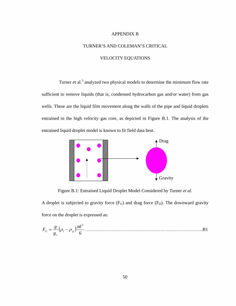
Turner et al.3 analyzed two physical models to determine the minimum flow rate

sufficient to remove liquids (that is, condensed hydrocarbon gas and/or water) from gas

wells. These are the liquid film movement along the walls of the pipe and liquid droplets

entrained in the high velocity gas core, as depicted in Figure B.1. The analysis of the

entrained liquid droplet model is known to fit field data best.

Drag

Gravity

Figure B.1: Entrained Liquid Droplet Model Considered by Turner et al.

A droplet is subjected to gravity force (FG) and drag force (FD). The downward gravity

force on the droplet is expressed as:

( )6

3dggF gl

cG

πρρ −= …………………………….……………………………………………...B1

50

The upward drag force is as follow:

( 2

21

dgddgc

D VVACg

F −= ρ ) ………………………………………………………………….....B2

Equating Equations B1 and B2 yields the terminal velocity (in ft/s):

gd

gldgt C

dVVV

ρρρ )(

55.6)(−

=−= …………………………………..…………………B3

Hinze12 showed that the droplet diameter (d) can be expressed in terms of the

dimensionless Weber Number (NWE) such that:

σρ

c

gtWE g

dVN

2

= ……………………………………………………………..……………B4

Hinze posited that the largest droplet occurs at NWE in the value range 20-30 and at NWE

greater than 30, the droplet will shatter. Hence the expression for the largest droplet

diameter, occurring at NWE of 30, is:

230tg

c

Vg

dρσ

= ……………………………………………………………………….……B5

The coefficient of discharge (Cd) is assumed to be approximately at 0.44 for

Reynolds number ranging from 1,000 to 200,000 (Newton’s Law region), as shown in

Figure 4.4. Having the interfacial tension (σ ) unit changed from pound force per foot

(lbf/ft) to dyne/cm (1lbf/ft = 0.00006852 dyne/cm) and substituting Cd of 0.44 and σ =

1lbf/ft = 0.00006852 dyne/cm with Equation B5 into Equation B3:

( )2

1

414

15935.1

g

gltV

ρ

ρρσ −= …………………………………………..…………..………………B6

51

The gas density expression is:

zTP

zRTMP

zRTPM gga

g

×≈

×==

γγρ 715.2

)(…………………………….………………...B7

For =gγ 0.6, T = 120 oF and z = 0.9, Equation (B7) will yield:

PPg 0031.0

9.0)120460(6.0715.2 =

×+×=ρ …………………..………………………B8

Typical values of density and interfacial tension for both water and gas condensate are:

=wρ 67 lbm/ft3

=condensateρ 45 lbm/ft3

=wσ 60 dyne/cm

=condensateσ 20 dyne/cm

Redefining the critical velocity (Vc) as the maximum terminal velocity of a

freely falling body in a fluid medium under the influence of gravity alone and substituting

the typical values of density and interfacial tension together with Equation B8 into

Equation B6, the Turner et al.3 and the Coleman et al.4 equations are expressed as:

(max)tc VV = ……………………………………...…………………………..……………B9

Turner et al.3 equations (with 20% adjustment to fit data):

( )( ) 2

1

41

,0031.0

0031.067304.5P

PV wc−

= ……………………………………………..…………..B10

( )( ) 2

1

41

,0031.0

0031.04503.4P

PV condc−

= ……………………………………………..………….B11

52

Coleman et al.4 equations (without any adjustment to fit data):

( )( ) 2

1

41

,0031.0

0031.067434.4P

PV wc−

= ………………………………………………..………..B12

( )( ) 2

1

41

,0031.0

0031.045369.3P

PV condc−

= ……………………………………………..………...B13

The critical velocity is easily translated to critical rate using the following expression:

zTVPA

q ct

)460(06.3+

= …………………………………………………………..………........ B14

53

APPENDIX C

LI’S CRITICAL VELOCITY EQUATIONS

Li, Li, and Sun6 argued that a pressure difference exists between the fore and aft

portions of a free falling droplet. The droplet is thus deformed, under the applied forces,

from a sphere to a convex bean (or a flat-shaped droplet). This is depicted in Figure C.1.

Figure C.1: Li’s Critical Velocity Model Using a Flat-Shaped Droplet6

Equating the gravity of a liquid droplet to the buoyancy and drag force, we obtain (in S.I

Units):

dggl sCvgVgV 2

21 ρρρ += ………………………………………………………........C1

Where:

lρ = liquid density, kg/m3

54

gρ = gas density, kg/m3

V = volume of liquid droplet, m3

g = acceleration due to gravity, m/s2

v = velocity, m/s

s = area of deformed droplet, m2

Cd = drag coefficient

As the droplet falls relative to the gas stream velocity, the pressure difference

existing between the fore and aft portions, by Bernoulli, is expressed as:

23

210

vp gρ−

=Δ ………………………………………………..………………………...C2

The condition for the balance of pressure and interfacial tension forces is:

010 3 =Δ+Δ⎟

⎠⎞

⎜⎝⎛ Δ

− shsp σ ……………………………………………………..……………..C3

For a constant volume of the droplet, the following conditions must be satisfied:

V = sh = constant………………………………………………………………..…….…C4

Where:

h = thickness of the droplet in the direction of motion

From Equation C3, we obtain:

hss

ΔΔ

=Δ− σρ310

………………………………………………………………..…………....C5

From Equation C4, we have:

55

hs

hsh

hV

hs

−=−=−=ΔΔ

22 ……………………………………………………….………..C6

By combining Equations C5 and C6, we calculate the thickness of the droplet as:

ph

Δ=

− σ310 ……………………………………….………………………………………C7

Substituting from Equation C2 into Equation C7, we have: pΔ

2

2v

hgρσ

= ……………………………….……………………………………………….C8

Hence, s is estimated to be:

σρ

2

2Vvs g= ……………………………………………………………………….…..….C9

Substituting Equation C9 into Equation C1 and solving for v = vc:

( )4 2

4

dg

glc C

gvv

ρσρρ −

== ………………………………………….…………………...C10

For a typical field condition, the particle’s Reynolds number ranges from 104 to

105 and the drag coefficient (Cd) is close to 1.0 for the shape considered. Hence, we have:

( )( ) 2

1

414

1

5.2g

glcv

ρ

ρρσ −= …………………………………………..……………...…….C11

zTApvq c

c5105.2 ×= ………………………………………..……………..…………….C12

The density of gas is determined by the expression:

zTpg

g

γρ 4844.3= …………………………………………………………….…..…….C13

With T measured in degree Kelvin.

56

For a gas gravity ( gγ ) of 0.6 and within the pressure range (4,500 – 23,000 kPa

or 653 – 3,350 psia) of Li’s field data, the average z is 0.85. The typical wellhead

temperature is given as 322oK. Substituting these data into Equation C13, we obtain:

pg 00764.0=ρ ………………………………….……………………………….…….C14

Taking water density ( lρ ) of 1074 kg/m3, a typical value of interfacial tension between

water and gas ( wσ ) of 0.06 N/m and z value of 0.85 into Equations C11 and C12

respectively, we obtain:

( )( ) 2

1

41

00764.000764.010742373.1p

pvc−

= …………………….………………………………...C15

( )( )

4

21

41

1000764.0

00764.01074113.0 ×

−×=

p

ppAq t

c .......................…….............................…...C16

Where:

At = area of tubing, m2

57

APPENDIX D

NOSSEIR’S CRITICAL VELOCITY EQUATIONS

Nosseir et al.7 assumed the droplet model and analyzed the downward

gravitational force and the upward drag force on the model. The gravitational force,

pulling the droplet downwards is expressed by the term:

( cglg gdF ρρπ−=

6

3

) ………………………….……………………………………..…D1

The drag force pushing the droplet upwards is expressed by the term:

42

22 dVCF cldd

πρ= …………………………………….…………………..……………..D2

A historical review of past analytical equations for different flow conditions is

carried out. For laminar flow regime, Stokes, in 1851, introduced his equation for

calculating the critical velocity (Re< 1):

lc

gd dV

Cρμ24

= ………………………………………………..………………….………....D3

The drag force is calculated:

cgd VdF μπ3= ……………………….…………………………………...……….…….. D4

Combining Equations D1 and D4, the terminal velocity equation reduces to Stokes Law:

( )g

glcc

dgV

μρρ

18

2 −= ………………..…………….………………………………………D5

58

Stokes’ Law applies better to small impure fluid particles, which is probably the case in

gas wells.

The drag coefficient equation of a gradually developing turbulence region (1 <

Re < 1000) is expressed as:

( ) 625.0Re30 −=dC ……………………………………………………….………………..D6

Hence the terminal velocity will reduce to:

( )45.0

18.172.0

2.0

⎟⎠⎞

⎜⎝⎛

∗⎪⎭

⎪⎬⎫

⎪⎩

⎪⎨⎧ −

=

g

gg

glc

dgV

ρμρ

ρρ……………..……………………..………….....D7

The turbulent flow regime extends from a Reynolds number (Re) of about 1,000

to 200,000 where the drag coefficient is fairly constant (Figure 4.4) at approximate Cd of

0.44. The terminal velocity equation can be described by one form of Newton’s Law:

( ) 5.0

5.074.1⎪⎭

⎪⎬⎫

⎪⎩

⎪⎨⎧ −

=g

glcc gdV

ρρρ

………………..………………………….…………...….D8

Nosseir et al.7 examined Turner’s initial assumptions, particularly the

dominance of Turbulent flow regime in a certain range, which determines the shape of

the drag coefficient and subsequently the critical velocity equation. They showed that

most of Turner’s data points fall in the highly turbulent region where Re exceeds the

value of 200,000. This region is termed ‘the highly turbulent flow regime’ with Re

extending from 200,000 to 106 with an average drag coefficient of 0.2. This is shown in

Figure D.1.

59

Figure D.1: Dependence of Drag Coefficient on Reynolds Number7

They again confirmed that most of Coleman’s data points fall in the Re range of 1000 to

200,000 and its corresponding Cd of 0.44. They argued that this is the reason why

Turner’s initial equation has a good match for Coleman’s data without adjustment.

Nosseir et al.7 went on to develop two analytical models, employing the hard,

smooth, spherical droplet of liquid, for the transition and highly turbulent flow regimes.

The transition flow equation is developed by substituting Hinze’s12 expression into

Equation D7:

( ) 72.0

45.0

18.1

2

*

302.0

⎪⎭

⎪⎬⎫

⎪⎩

⎪⎨⎧ −

⎟⎟⎠

⎞⎜⎜⎝

⎛

⎪⎭

⎪⎬⎫

⎪⎩

⎪⎨⎧

=g

glc

g

g

gc

c

c gV

g

Vρρρ

ρμ

ρσ

…………..………………………..……….. (D9)

60

( ) ( ) 45.036.218.118.1

72.0

///** ggcgg

glcc V

gKV ρμρσ

ρρρ

⎪⎭

⎪⎬⎫

⎪⎩

⎪⎨⎧ −

= …………...………….….... (D10)

Where:

K = 0.2* (32.17)0.72 * (30)1.18 * (32.17)1.18 = 8094.5

( ) 45.018.118.1

72.0

36.3 ///** gggg

glc KV ρμρσ

ρρρ

⎪⎭

⎪⎬⎫

⎪⎩

⎪⎨⎧ −

= …..………………………..…….. (D11)

( ) 134.035.035.0

21.0

36.3136.3 ///** ggg

g

glc KV ρμρσ

ρρρ

⎪⎭

⎪⎬⎫

⎪⎩

⎪⎨⎧ −

= ……..……………..…….…. (D12)

( )426.0134.0

21.035.06.14

gg

glcV

ρμρρσ −

= ………………….………………………………..…...…. (D13)

Equation D13 is the Nosseir et al.7 critical velocity equation for flow under transition

flow regime.

The derivation of critical velocity equation for the highly turbulent flow regime

follows equally. Starting from Equations D1 and D2, and substituting for maximum

diameter by Hinze12, we obtain:

( )cg

glc V

Vρ

σρρ 5.05.067.454 −= …………..…………………...………….………..…… (D14)

Solving for Vc yields:

( )5.0

25.025.03.21

g

glcV

ρρρσ −

= ……….……………………………..…………………... (D15)

61

PERMISSION TO COPY

In presenting this thesis in partial fulfillment of the requirements for a master’s

degree at Texas Tech University or Texas Tech University Health Sciences Center, I

agree that the Library and my major department shall make it freely available for

research purposes. Permission to copy this thesis for scholarly purposes may be granted

by the Director of the Library or my major professor. It is understood that any copying

or publication of this thesis for financial gain shall not be allowed without my further

written permission and that any user may be liable for copyright infringement.

Agree (Permission is granted.)

___________Awolusi________________________________ __07/31/2005______ Student Signature Date Disagree (Permission is not granted.) _______________________________________________ _________________ Student Signature Date