Resolving subtle stratigraphic features using spectral ridgesand phase residues

Oswaldo Davogustto1, Marcílio Castro de Matos1, Carlos Cabarcas1, Toan Dao1, and Kurt J. Marfurt1

Abstract

Seismic interpretation is dependent on the quality and resolution of seismic data. Unfortunately, seismicamplitude data are often insufficient for detailed sequence stratigraphy interpretation. We reviewed a methodto derive high-resolution seismic attributes based upon complex continuous wavelet transform pseudodecon-volution (PD) and phase-residue techniques. The PD method is based upon an assumption of a blocky earthmodel that allowed us to increase the frequency content of seismic data that, for our data, better matched thewell log control. The phase-residue technique allowed us to extract information not only from thin layers butalso from interference patterns such as unconformities from the seismic amplitude data. Using data from aWestTexas carbonate environment, we found out how PD can be used not only to improve the seismic well ties butalso to provide sharper sequence terminations. Using data from an Anadarko Basin clastic environment, wediscovered how phase residues delineate incised valleys seen on the well logs that are difficult to see on verticalslices through the original seismic amplitude.

IntroductionFourier spectral analysis is a key component of

seismic data processing. Random and coherent noisefiltering, spectral balancing, wavelet shaping, and Qcompensation are all based on spectral analysis. Spec-tral analysis techniques are also useful in seismic inter-pretation. Using a running window spectral analysis,also called a short window discrete Fourier transform(SWDFT), Partyka et al. (1999) compute the spectrafor overlapping windows thereby producing a 4Dtime-frequency data volume. These 4D frequency datavolumes can be used to detect lateral changes in thick-ness. In addition to the SWDFT, one can use transformsbased on a library of wavelets, giving rise to the continu-ous wavelet transform (CWT) (e.g., Stockwell trans-forms) and matching pursuit algorithms (Castagnaet al., 2003).

Taner et al. (1979) introduce complex trace attrib-utes such as quadrature, envelope, phase, and instanta-neous frequency, attributes that are well known amongthe geophysical community. Taner et al. (1979) notethat the instantaneous frequency f suffered discontinu-ities associated with abrupt changes in phase, which inturn were associated with waveform interference lo-cated at envelope e minima. To remove these disconti-nuities, Taner et al. (1979) introduce a weighted averagefrequency f avg at time t ¼ kΔt as

f avgk ¼PþK

j¼−K ek−jf instk−jLjPþK

j¼−K ek−jLj; (1)

where e is the envelope (also called the reflectionstrength), f inst is the instantaneous frequency, and Lis a low-pass filter.

Combining the concepts of instantaneous andweighted average frequency, Taner (2000) introducesa thin-bed indicator attribute by removing theweighted average frequency from the instantaneous fre-quency thereby enhancing zones in which waveletdestructive interference takes place. The thin-bed indi-cator is given by

f thin ¼ f inst − f avg: (2)

These zones of destructive interference are referredto as frequency spikes. In Figure 1, we show an exampleof the instantaneous frequency, weighted average fre-quency, and thin-bed indicator attributes.

Zeng (2010) uses synthetic models and field data tocorrelate frequency spikes with geologic information,defining two types of frequency spikes. Type I spikesare related to the destructive interference of the topand base layer reflection of a wedge. Type II spikesare more indicative of thin beds. Zeng (2010) shows

1University of Oklahoma, ConocoPhillips School of Geology and Geophysics, USA. E-mail: dellpi@ou.edu; marcilio@matos.eng.br; cabarcas@ou.edu; toandaogphy@ou.edu; kmarfurt@ou.edu.

Manuscript received by the Editor 22 February 2013; revised manuscript received 16 May 2013; published online 7 August 2013. This paperappears in INTERPRETATION, Vol. 1, No. 1 (August 2013); p. SA93–SA108, 21 FIGS.

http://dx.doi.org/10.1190/INT-2013-0015.1. © 2013 Society of Exploration Geophysicists and American Association of Petroleum Geologists. All rights reserved.

t

Special section: Interpreting stratigraphy from geophysical data

Interpretation / August 2013 SA93

type II spikes occur at wavelengths less than one-fifth ofa wavelength (Figure 2).

Li and Liner (2008) introduce a technique based onthe Hough transform to detect singularities in the CWTmagnitude spectra. Using Li and Liner’s (2008) algo-rithm, Smythe et al. (2004) show that discontinuitiesin the CWT of the underlying impedance model are pre-served as discontinuities seen in band-limited seismicamplitude data.

In general, seismic data amplitudes are not as wellpreserved as seismic phases. Matos et al. (2011) there-fore introduce an alternative spectral discontinuitymethod based on the phase of the CWT components.Because instantaneous frequency is the time derivativeof the instantaneous phase, there is a direct relationshipbetween Matos and Marfurt (2011) phase discontinuity

and earlier work by Taner (2000) and Zeng (2010). Like-wise, there is a similarity between (Matos and Marfurt,2011) pseudodeconvolution (PD) and “spectral whiten-ing” deconvolution operators implemented in the fre-quency domain.

We begin our paper with a review of spectral decom-position to generate PD and phase residues attributes.

Figure 1. Vertical slices through (a) instantaneous frequencyf inst, (b) envelope weighted average frequency, f avg, and(c) thin-bed indicator, f thin ¼ f inst-f avg obtained as the differ-ence between the (a and b). (c) Is plotted using a color barthat highlights the extreme values (after Taner, 2000).

Figure 2. Zeng’s (2010) (a) seismic amplitude and (b) corre-sponding instantaneous frequency from a three-layer modelgiving rise to a reflector coefficient of −R and +R for the firstand second interface. Note the “type I” spikes within thecenter layer. (c) Seismic amplitude and (d) corresponding in-stantaneous frequency for a seven-layer model giving rise to asuite of −R, +R, −R, +R, −R, +R, reflection coefficients be-tween interfaces. On these models, two types of frequencyspikes can be identified. (b) Zeng (2010) defines the anomalyobserved at the center of the model as a type I spike. Note thatthe spike appears at wavelengths larger than tuning wave-length. (d) Zeng (2010) finds that type II spikes are associatedwith thin beds, they depend on the impedance contrast of thelayers, and the predominant wavelet frequency in which theyoccur is inversely proportional to the thickness of the beds.

SA94 Interpretation / August 2013

We then apply these methods to a carbonate systemfrom West Texas and show how these algorithms canhelp accelerate interpretation of thin reflectors. Then,we apply these algorithms to a Red Fork incised valleysystem from the Anadarko Basin and show how phaseresidues correlate to sequence boundaries seen on logs.We conclude with a discussion of assumptions, process-ing workflows, and limitations associated with thesetwo attributes.

Methodology reviewSpectral ridges and PD

The CWT is the crosscorrelation between the seismictrace and dilated versions of a symmetric “mother”wavelet (Grossman and Morlet, 1984). Because themother wavelet is symmetric, we can compute theCWT by convolving the seismic trace with the time-reversed scaled version of the basic wavelet (Figure 3c).Because convolution in the time domain is equivalent tomultiplication in the frequency domain, we can also in-terpret the CWT as a suite of band-pass filters resultingin spectral components. Each seismic trace is repre-

sented by a time (depth) versus frequency band (orscale) complex matrix. This matrix represents how wellthe seismic trace correlates to each dilated wavelet ateach instant of time (Matos and Marfurt, 2011).

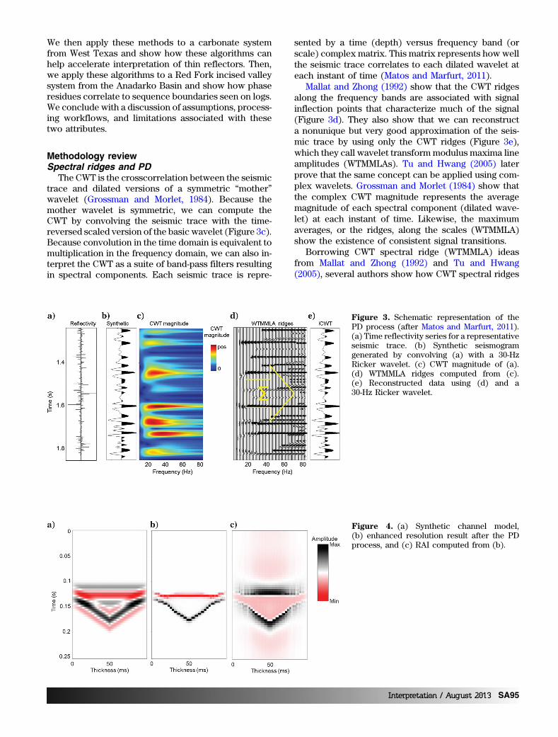
Mallat and Zhong (1992) show that the CWT ridgesalong the frequency bands are associated with signalinflection points that characterize much of the signal(Figure 3d). They also show that we can reconstructa nonunique but very good approximation of the seis-mic trace by using only the CWT ridges (Figure 3e),which they call wavelet transformmodulus maxima lineamplitudes (WTMMLAs). Tu and Hwang (2005) laterprove that the same concept can be applied using com-plex wavelets. Grossman and Morlet (1984) show thatthe complex CWT magnitude represents the averagemagnitude of each spectral component (dilated wave-let) at each instant of time. Likewise, the maximumaverages, or the ridges, along the scales (WTMMLA)show the existence of consistent signal transitions.

Borrowing CWT spectral ridge (WTMMLA) ideasfrom Mallat and Zhong (1992) and Tu and Hwang(2005), several authors show how CWT spectral ridges

Figure 3. Schematic representation of thePD process (after Matos and Marfurt, 2011).(a) Time reflectivity series for a representativeseismic trace. (b) Synthetic seismogramgenerated by convolving (a) with a 30-HzRicker wavelet. (c) CWT magnitude of (a).(d) WTMMLA ridges computed from (c).(e) Reconstructed data using (d) and a30-Hz Ricker wavelet.

Figure 4. (a) Synthetic channel model,(b) enhanced resolution result after the PDprocess, and (c) RAI computed from (b).

Interpretation / August 2013 SA95

can be associated with a reflectivity series (Hermannand Stark, 2000; Li and Liner, 2008; Devi and Schwab,2009; Matos and Marfurt, 2011). Matos and Marfurt(2011) show how to enhance seismic resolution by us-ing complex Morlet CWT spectral ridges and recon-structing the seismic trace using broader bandwavelets than those used in the original analysis givinga result they call PD. This process is schematicallyshown in Figure 3.

Figure 4a shows a single 2D synthetic seismic re-sponse of a channel with thicknesses varying from 0to 50 ms. Figure 4b shows the PD result. We can clearlysee the improvement in the seismic resolution. Figure 4cshows the relative acoustic impedance (RAI) computedfrom Figure 4b. This high-resolution seismic represen-tation can be considered a reflectivity approximation,which can be integrated to estimate the RAI (Berteus-sen and Ursin, 1983). The RAI computation consists ofthree steps:

1) rescale the high-resolution trace by keeping themagnitude much smaller (we suggest 10 times) thanone

2) integrate the trace using the procedure designed byPeacock (1979) for discrete integration

3) high-pass filter (we suggest f > 10 Hz) the inte-grated data to provide RAI.

We assume that the earth impedance model isblocky, thus giving rise to a suite of sparse spikes thatwe convolve with a narrowband seismic wavelet givingrise to conventional seismic data. We can replace thesewavelets frequency by frequency with their broadbandequivalents, thereby generating a broadband signal. Theprocess relies on the original frequency information ofthe narrowband wavelets; hence, the frequencies notsampled will not be reconstructed. We validate all theseassumptions by tying the broadband data to well syn-thetic seismograms.

Figure 5. (a) Amplitude from a three-layer synthetic wedge model. Corresponding CWT spectral magnitude response at (b) 15, (c)30, and (d) 70 Hz and phase response at (e) 15, (f) 30, and (g) 70 Hz. We identify phase anomalies in the spectral phase (whitearrows) and magnitude (black arrows). This is the phenomena that is first described by Ghiglia and Pritt (1998). Note that theanomaly location is frequency dependent.

SA96 Interpretation / August 2013

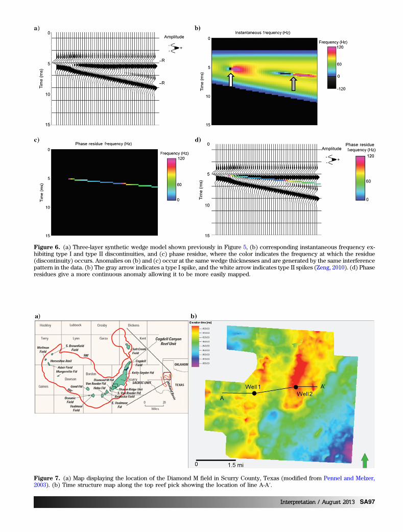
Figure 6. (a) Three-layer synthetic wedge model shown previously in Figure 5, (b) corresponding instantaneous frequency ex-hibiting type I and type II discontinuities, and (c) phase residue, where the color indicates the frequency at which the residue(discontinuity) occurs. Anomalies on (b) and (c) occur at the same wedge thicknesses and are generated by the same interferencepattern in the data. (b) The gray arrow indicates a type I spike, and the white arrow indicates type II spikes (Zeng, 2010). (d) Phaseresidues give a more continuous anomaly allowing it to be more easily mapped.

Figure 7. (a) Map displaying the location of the Diamond M field in Scurry County, Texas (modified from Pennel and Melzer,2003). (b) Time structure map along the top reef pick showing the location of line A-A′.

Interpretation / August 2013 SA97

Figure 8. Well 2 synthetic seismogram using the seismic amplitude data. The correlation was done using a 250-ms window cen-tered at 870 ms. The correlation coefficient is 68%. The green marker in the synthetic window corresponds to the top of the Horse-shoe Atoll reef. Note that the extracted wavelet is minimum phase.

Figure 9. Well 2 synthetic seismogram using the PD data. The correlation was done using a 250-ms window centered at 870 ms.The correlation coefficient is 79%. The green marker in the synthetic window corresponds to the top of the Horseshoe Atoll reef.Note that the extracted wavelet is zero phase.

SA98 Interpretation / August 2013

Spectral discontinuities and phase residuesAlthough the complex CWT phase can be used to re-

construct the high-resolution trace, Bone (1991) showsthat a shifted and dilated wavelet can interfere with an-other wavelet creating a signature in the phase spectra.This interference or inconsistency is called a phase res-idue. Matos et al. (2011) show how one can detectphase discontinuities in the Morlet complex wavelettransform phase component. They implement the tech-nique that Ghiglia and Pritt (1998) develop for detectingphase anomalies using a rectangular window and look-ing for inconsistent phase values when unwrappingthese phase components. Matos et al. (2011) use phaseresidues to map wavelet interference patterns that cor-relate with stratigraphic discontinuities as well as in-consistencies in seismic data quality. To demonstratethis concept, we generated a three-layer syntheticwedge model embedded in a shale background. We

used a Ricker wavelet with a peak frequency of46 Hz and 100 ms length. In Figure 5, we show the spec-tral magnitude and spectral phase for 15-, 30-, and 70-Hzfrequencies for our wedge model. We are able to iden-tify the phase discontinuities that Ghiglia and Pritt(1998) describe within each magnitude-phase panefor each frequency. Figure 6 shows the phase residuesgenerated using the model shown in Figure 5.

Note that the discrete type I and type II spikes seen inFigure 6 appear as a more continuous anomaly in thephase residue seen in Figure 6c, allowing one to trackthe discontinuity laterally. Cohen (1993) shows that in-stantaneous attributes estimate the average propertiesof the seismic wavelet, such as the instantaneous fre-quency of an isolated wavelet. Note that type I and typeII discontinuities appear at approximately 60 Hz(green). Examining Figure 6c, we note the phase resi-due at these two locations also occurs at 60 Hz (green).

Figure 10. Cross section A-A′ displaying wells 1 and 2 converted to time using the time to depth relationship from the PD seismicwell tie (Figure 9). (a) Although the time to depth relationships were created using the PD data, these relationships work well withthe seismic amplitude data too. Log curves on the wells are gamma ray (black), bulk density (red), and neutron porosity (blue). Thegamma ray values increase to the left, and the bulk density and neutron porosity values increase to the right. (b) PD data crosssection A-A′ displaying wells A and B converted to the time to depth relationship from the PD seismic well tie (Figure 9). With thePD data, it is easier to identify onlaps, toplaps, downlaps, and reflector truncations than with the seismic amplitude data. (c) PDdata cross section A-A′ zoomed on the clinoform interval. Black arrows indicate downlap or onlap features identified in the internalstructure of the clinoform. On well 2, we identify a highstand to transgressive system track sequence (green arrow) that correlateswith our onlap and downlap features. Note that the same event is not identified on well 1, indicating that well 1 is closer to the shelf.(d) Seismic amplitude data cross section A-A′ zoomed on the clinoform interval. Besides the onlap features close to well 1, it isdifficult to identify any other clear reflector terminations in the seismic amplitude data.

Interpretation / August 2013 SA99

Figure 11. (a) RAI volume probe with all vox-els in the probe plotted as opaque. We will useopacity on the histogram to isolate the responseof the top (magenta) and base (red) of the pro-grading sequence shown in Figure 10. Note thatthe clinoform has a distinctive response beingdelimited by the highest and lowest values ofRAI. (b) Setting the low-amplitude voxels asopaque isolates the top boundary of the clino-form. (c) Setting the high-amplitude voxels asopaque isolates the bottom boundary of the cli-noform. We use these two geobodies as inputfor out seismic interpretation.

Figure 12. (a) Using the geobody extractionshown in Figure 11b and 11c, we convert thetop and bottom of the prograding sequence tothe green and yellow seismic horizons. We inter-pret the green horizon as a maximum floodingsurface (MFS) and the yellow horizon as a se-quence boundary (SB). This interpretation is cor-roborated by the results found in Figures 10 and11. (b) Comparison of the RAI volume to theacoustic impedance log from wells 1 and 2.The AI log decreases to the right. At the zoneof interest, the acoustic impedance log showsan excellent correlation with the RAI attribute,demonstrating that the RAI algorithm is reliable,and it can be used in frontier zones where wellsare not present to delineate zones of interest.

SA100 Interpretation / August 2013

Rather than probing for discontinuities at the averagefrequency, the phase residue algorithm probes at a suiteof frequencies on CWT spectral components, therebygiving rise to a laterally continuous anomaly.

Comparing Figures 4 and 6, we see the complemen-tary nature of CWT phase residues, high-resolutionspectral ridges and RAI and their potential use in seis-mic interpretation. Specifically, spectral ridges enhanceindividual reflectors, whereas phase residues enhanceunconformities and pinch-outs.

Application of CWT attributes to improve reservoirgeometry interpretationCarbonate environment example(Midland Basin, TX)

The Diamond M data set consists of approximately25 mi2 of seismic data with a high signal-to-noise ratiolocated in Scurry County, TX (Figure 7). We computedthe PD and RAI attributes to determine if they betterdefine the stratigraphic sequences of interest. Figure 7shows the location of the composite seismic line and

the location of two wells used for the interpretation.Figures 8 and 9 show representative synthetic seismo-grams used to tie well data to the original seismic dataand PD data, respectively. The original data show a min-imum phase character, whereas the bandwidth exten-sion process not only enhances the resolution of thedata but also converts it to zero phase. Examiningcomposite line AA′ we compare the original seismicdata with the PD data in our integrated interpretationwith the well data (Figure 10). We identify reflector ter-minations on Figure 10b in the vicinity of well 2 that onFigure 10a appear as a continuous reflector. Furtherevaluation using the well logs allows us to interpretthe sequence as a highstand to transgressive systemstrack progression (Figure 10c). We compared the PDand seismic amplitude data and found that the PD datashows a better defined progradational sequence withinternal onlap and downlap terminations for the identi-fied sequence (Figure 10c–10d). We proceed to evaluatethe RAI character of this clinoform using a seismicprobe, and we are able to extract the top and the baseof the clinoform sequence and convert them to seismic

Figure 13. (a) Location of the Watonga data set in the Anadarko Basin, OK (after Peyton et al., 1998). (b) Representative horizonthrough seismic amplitude at the top Pink Lime indicating the location of composite line AA′. (c) Red Fork incised valley stages Ithrough V (after Peyton et al., 1998).

Interpretation / August 2013 SA101

horizons (Figure 11). We display our RAI-createdhorizons on the original seismic data and the PD(Figure 12a) data and corroborate that the top and basehorizons correspond to the previously identified high-stand systems tract sequence. Finally, we comparethe RAI result to the acoustic impedance (AI) log find-ing a strong correlation (Figure 12b). This result dem-onstrates the reliability of the RAI using the CWTmethod in areas where little or no well control is avail-

able. Equally important, generating the horizons usingPD, RAI, and geobody extraction took 30 minutes ver-sus 3 hours using the conventional autotracker seismicinterpretation.

Clastic environment example(Anadarko Basin, OK)

Red Fork sands are a prominent gas producer in theAnadarko Basin. The Red Fork stratigraphy consists of

Figure 14. (a) Stratigraphic well log cross section A-A′. Based on the well log data and the interpreted well tops, we define fiveincision stages on the Red Fork formation. This interpretation is similar to that of Peyton et al. (1998). (b-d) Zoomed portions of A-A′ cross section. Data and cross-section interpretation are courtesy of M. Falk and A. Warner, Chesapeake Energy Corp.

SA102 Interpretation / August 2013

regional deltaic deposits that endured five stages of flu-vial incision during a sea-level low stand. Such fluvialincisions are informally called invisible channels be-cause they cannot be identified on stacked seismic databut are encountered by subsequent drilling to deepertargets (Peyton et al., 1998; Suarez et al., 2008; Barber,2010).

Figure 13 shows a map with the location of the seis-mic data of the Watonga field, well locations, andcomposite line locations and the Peyton et al. (1998)interpretation of the Red Fork incised valleys usingsemblance, 30-Hz spectral magnitude, and well data.Collaborating with Chesapeake Energy geoscientists,

we show an updated version of Peyton et al.’s (1998)cross-section AA′ using the exact same well data (Fig-ure 14). Figures 15 and 16 show the synthetic seismo-grams for wells R and S, respectively. These are the onlywells with sonic and density logs in the survey. Well Rpenetrates the regional Red Fork sequence. Well S pen-etrates incision stage V. Time to depth curves differ de-pending on the geologic section that a well penetrates.We found that wells that penetrate the regional RedFork share a similar time to depth relationship, whereaswells that penetrate any of the incision stages share adifferent time to depth relationship. By using these twodifferent time to depth curves, we were able to tie most

Figure 15. Well R synthetic seismogram us-ing the seismic amplitude data. The correla-tion was done using a 250-ms windowcentered at 1800 ms. The correlation coeffi-cient is 70%. Orange marker corresponds tothe Oswego Limestone. The yellow markercorresponds to the Inola Limestone, and thegreen marker in the synthetic window corre-sponds to the top of the Novi Limestone.

Figure 16. Well S synthetic seismogram us-ing the seismic amplitude data. The correla-tion was done using a 300-ms windowcentered at 1800 ms. The correlation coeffi-cient is 70%. The orange marker correspondsto the Oswego Limestone. The pink markercorresponds to the base of the Pink Lime,and the green marker in the synthetic windowcorresponds to the top of the Novi Limestone.

Interpretation / August 2013 SA103

wells on Peyton et al.’s (1998) AA′ cross sectionwith our seismic amplitude and phase residue data.Composite line AA′ through the seismic data showsone of these incisions (Figure 17). Once we tied allthe wells in Figure 14 with the seismic data, we com-pared the well tops from the regional Red Fork andthe incision stages with anomalies observed in the seis-mic data. In the seismic amplitude section, we are able

to correlate only the Pink Lime, Inola Limestone, andstage V tops (Figure 17b and 17c). Using phase residuesand the regional Red Fork and incision stage tops fromFigure 14, we not only identify the stage V incision as inFigure 17, but we are also able to identify two additionalphase residue anomalies that correspond to the otherstages of incision that were invisible on the seismic data(Figure 18b and 18c). We proceed to interpret the phase

Figure 17. Vertical section AA′ through(a) seismic amplitude data, (b) seismic ampli-tude data with Pink Lime (pink horizon) andInola Limestone (blue horizon) interpreted onthe seismic amplitude data using the guidancefrom the well-top data, and (c) interpretedseismic amplitude data with incision stageswell-tops overlaid. (a) We are able to identifyincision stage V between wells S and U, butstages I–IV are invisible on the seismic ampli-tude data. (b) We interpreted the Pink Limeand Inola Limestone (pink and blue horizons,respectively) and posted the interpreted topsfor the same surfaces in each well to corrobo-rate our interpretation. (c) By posting the in-terpreted incision stages surfaces for the welldata, we corroborate that stages I–IV of inci-sion are invisible on seismic vertical sections.

Figure 18. Vertical section AA′ through(a) phase residues attribute, (b) phase resi-dues with regional Red Fork the well-top dataposted, and (c) phase residues with incisionstages well tops posted. (a) On the phase res-idues attribute we identify anomalies thatresemble channel like features. (b-c) We cor-roborate that some of the anomalies seen in(a) match the interpreted regional Red Fork(diamond shapes) as well as the incisionstages (square shapes) from the well logs.

SA104 Interpretation / August 2013

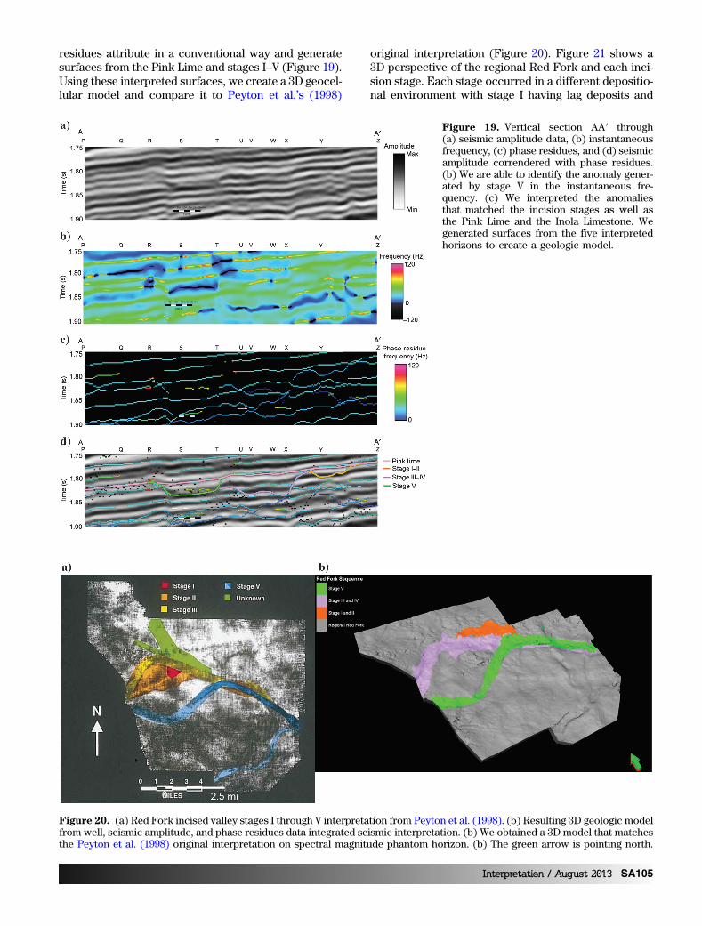
residues attribute in a conventional way and generatesurfaces from the Pink Lime and stages I–V (Figure 19).Using these interpreted surfaces, we create a 3D geocel-lular model and compare it to Peyton et al.’s (1998)

original interpretation (Figure 20). Figure 21 shows a3D perspective of the regional Red Fork and each inci-sion stage. Each stage occurred in a different depositio-nal environment with stage I having lag deposits and

Figure 19. Vertical section AA′ through(a) seismic amplitude data, (b) instantaneousfrequency, (c) phase residues, and (d) seismicamplitude correndered with phase residues.(b) We are able to identify the anomaly gener-ated by stage V in the instantaneous fre-quency. (c) We interpreted the anomaliesthat matched the incision stages as well asthe Pink Lime and the Inola Limestone. Wegenerated surfaces from the five interpretedhorizons to create a geologic model.

Figure 20. (a) Red Fork incised valley stages I through V interpretation from Peyton et al. (1998). (b) Resulting 3D geologic modelfrom well, seismic amplitude, and phase residues data integrated seismic interpretation. (b) We obtained a 3D model that matchesthe Peyton et al. (1998) original interpretation on spectral magnitude phantom horizon. (b) The green arrow is pointing north.

Interpretation / August 2013 SA105

stage V filled by a shale plug (Suarez et al., 2008).Separating each stage from the regional Red Forkfacilitates geologic modeling each stage to estimatereservoir properties consistent with the depositionalenvironment.

ConclusionsSpectral analysis has long been used in seismic

processing and interpretation. We have demonstratedhow CWT PD, RAI, and phase residues can be effec-tively applied to reveal and enhance stratigraphicfeatures that are buried in conventional seismic ampli-tude data. PD enhances reflector terminations, facilitat-ing seismic sequence stratigraphy interpretation. RAIcomputed from PD, when used as a geobody extractionand interpretation tool, accelerates the interpretationof clinoforms and complex features. Phase residuesextends the well established thin bed indicator and in-stantaneous frequency spike interpretation workflows,providing more continuous discontinuities, as well asthe magnitude and frequency at which they occur.We have developed a workflow that combines seis-mic amplitude with CWT attributes to produce a high-frequency seismic stratigraphy framework for seismicinterpretation. Finally, we have demonstrated how bycombining CWT attributes with detailed seismic stratig-

raphy, sequences can be extracted from the seismicdata as an input for detailed reservoir characterization.

AcknowledgmentsThe authors would like to thank Chesapeake Energy

Corporation for providing a license to well data and theoriginal version of the seismic data and M. Falk and A.Warner for their contribution to understanding the com-plex geology of the Red Fork formation. We thankCGGVeritas for providing a license to the reprocesseddata that forms part of a mega merge survey. We thankParallel Petroleum LLC for providing a license to theDiamond M data set and Alison Small for her invaluablehelp on interpretation of the Diamond M data. We thankSchlumberger for donating the Petrel software for usein research and education. We thank H. Zeng, D. Gao, B.Hart, and Y. Sun whose careful reviews and detailedcomments helped improve this paper. Finally, we wouldlike to thank A. Miceli, J. T. Kwiatkowski, B. C. Wallet,R. Brito, and R. Slatt for their help and support.

ReferencesBarber, R., 2010, Challenges in mapping seismically in-

visible Red Fork channels: Shale Shaker Digest, 61,147–162.

Figure 21. Three-dimensional view of (a) regional Red Fork, (b) incision stages I and II, (c) incision stage III and IV and (d) in-cision stage V obtained from the integrated seismic interpretation. Separating each stage from the regional Red Fork facilitates thegeologic modeling of each stage to estimate reservoir properties consistent with the depositional environment.

SA106 Interpretation / August 2013

Berteussen, K. A., and B. Ursin, 1983, Approximate com-putation of the acoustic impedance from seismic data:Geophysics, 48, 1351–1358, doi: 10.1190/1.1441415.

Bone, D. J., 1991, Fourier fringe analysis: The two-dimensional phase unwrapping problem: AppliedOptics, 30, 3627–3632, doi: 10.1364/AO.30.003627.

Castagna, J., S. Sun, and R. Siegfried, 2003, Instantaneousspectral analysis: Detection of low-frequency shadowsassociated with hydrocarbons: The Leading Edge, 22,120–127, doi: 10.1190/1.1559038.

Cohen, L., 1993, Instantaneous “anything”: IEEEInternational Conference on Acoustics, Speech, andSignal Processing, 1993. ICASSP-93: IEEE, 4, 105–108.

Devi, K. R. S., and H. Schwab, 2009, High-resolution seis-mic signals from band-limited data using scaling laws ofwavelet transforms: Geophysics, 74, no. 2, WA143–WA152, doi: 10.1190/1.3077622.

Ghiglia, D., and M. D. Pritt, 1998, Two-dimensional phaseunwrapping: Theory, algorithms, and software: Wiley-Interscience.

Grossmann, A., and J. Morlet, 1984, Decomposition ofHardy functions into square integrable wavelets of con-stant shape: SIAM Journal on Mathematical Analysis,15, 723–736, doi: 10.1137/0515056.

Herrmann, F., and C. Stark, 2000, A scale attribute for tex-ture in well and seismic data: 70th Annual InternationalMeeting, SEG, Expanded Abstracts, 2063–2066.

Li, C., and C. Liner, 2008, Wavelet-based detection of sin-gularities in acoustic impedances from surface seismicreflection data: Geophysics, 73, no. 1, V1–V9, doi: 10.1190/1.2795396.

Mallat, S., and S. Zhong, 1992, Characterization of signalsfrom multiscale edges: IEEE Transactions on PatternAnalysis and Machine Intelligence, 14, 710–732, doi:10.1109/34.142909.

Matos, M. C., O. Davogustto, K. Zhang, and K. J. Marfurt,2011, Detecting stratigraphic discontinuities using time-frequency seismic phase residues: Geophysics, 76,no. 2, P1–P10, doi: 10.1190/1.3528758.

Matos, M. C., and K. J. Marfurt, 2011, Inverse continuouswavelet transform “deconvolution”: 81st AnnualInternational Meeting, SEG, Expanded Abstracts,1861–1865.

Partyka, G., J. Gridley, and J. Lopez, 1999, Interpretationalapplications of spectral decomposition in reservoircharacterization: The Leading Edge, 18, 353–360, doi:10.1190/1.1438295.

Peacock, K. L., 1979, An optimum filter design for discreteintegration: Geophysics, 44, 722–729, doi: 10.1190/1.1440972.

Pennell, S., and S. Melzer, 2003, Oxy Permian’sCogdell Unit CO2 flood responds rapidly to CO2 injec-tion: World Oil, http://www.worldoil.com/June-2003-Petroleum-Technology-Digest-Oxy-Permians-Cogdell-Unit-responds-rapidly-to-CO2-injection.html, accessedFebruary 2013.

Peyton, L., R. Bottjer, and G. Partyka, 1998, Interpretationof incised valleys using new 3-D seismic techniques: Acase study using spectral decomposition and coher-ency: The Leading Edge, 17, 1294–1298, doi: 10.1190/1.1438127.

Smythe, J., A. Gertsztenkorn, B. Radovich, C. F. Li, and C.Liner, 2004, Gulf of Mexico shelf framework interpreta-tion using a bed-form attribute from spectral imaging:The Leading Edge, 23, 921–926.

Suarez, Y., K. J. Marfurt, and M. Falk, 2008, Seismic attrib-ute-assisted interpretation of channel geometries andinfill lithology: A case study of Anadarko Basin RedFork channels: 78th Annual International Meeting,SEG, Expanded Abstracts, 963–967.

Taner, M. T., 2000, Attributes revisited, http://www.rocksolidimages.com/pdf/attrib_revisited.htm, accessed20 March 2013.

Taner, M. T., F. Koehler, and R. E. Sheriff, 1979, Complexseismic trace analysis: Geophysics, 44, 1041–1063, doi:10.1190/1.1440994.

Tu, C. L., and W. L. Hwang, 2005, Analysis of singularitiesfrom modulus maxima of complex wavelets: IEEETransactions on Information Theory, 51, 1049–1062,doi: 10.1109/TIT.2004.842706.

Zeng, H. L., 2010, Geologic significance of anomalous in-stantaneous frequency: Geophysics, 75, no. 3, P23–P30, doi: 10.1190/1.3427638.

Oswaldo Davogustto received a B.S.(2006) in geophysical engineeringfrom Universidad Simón Bolívar andan M.S. (2011) in geophysics fromthe University of Oklahoma, wherehe is pursuing his Ph.D. in explorationgeophysics. He worked as an acquisi-tion geophysicist in Lake Maracaibo,Venezuelan Gulf, and Orinoco Delta.

His research interests include fracture detection and char-acterization from seismic, log, and core data. For his dis-sertation he is working on processing and interpretation ofmulticomponent seismic focused on reservoir characteri-zation and properties prediction.

Marcílio Castro de Matos receiveda B.S. (1988) and an M.S. (1994) inelectrical engineering from InstitutoMilitar de Engenharia (IME) and adoctoral degree (2004) from PontificiaUniversidade Catolica do Rio de Ja-neiro. He served from 1989 to 1999as a military engineer at the BrazilianArmy Test Center and at IME as a

signal processing military professor from 1999 to 2010.He was a visiting scholar at the University of Oklahomafrom January 2008 to January 2010. He is currently coin-vestigator of the Attribute-Assisted Seismic Processing &

Interpretation / August 2013 SA107

Interpretation Research Consortium at the Universityof Oklahoma and is the principal of SISMO Signal Pro-cessing Research, Training & Consulting. His researchinterests include applied seismic analysis, digital signalprocessing, spectral decomposition, and seismic patternrecognition.

Carlos Cabarcas received degrees ingeophysics from the University ofOklahoma, l'Ecole National Superiordu Petrole et des Moteurs, and Univer-sidad Simón Bolívar. He also coordi-nates major geophysical efforts forHilcorp Energy Company, contribut-ing with his work to the ambitiousgoal of creating the premier private

energy company in America. He is a member of the entre-preneurs’ team that is currently building the premier pri-vate energy company of America. He started his careerin 1999 as a geophysical engineer trainee at Petróleosde Venezuela. Since then, he has expanded his formal ed-ucation and simultaneously gained hands-on experienceworking for Fusion Geophysical, Chesapeake Energy,and Chevron Energy Technology Company. He is an activemember of SEG, AAPG, and SPE.

Toan Dao received a B.S. (2010) andan M.S. (2013) in geophysics from theUniversity of Oklahoma. His researchinterests include signal processing,time-frequency analysis, and scientificcomputing.

Kurt J. Marfurt joined the Universityof Oklahoma in 2007, where he servesas the Frank and Henrietta SchultzProfessor of Geophysics within theConocoPhillips School of Geologyand Geophysics. His primary researchinterest is in the development and cal-ibration of new seismic attributes toaid in seismic processing, seismic in-

terpretation, and reservoir characterization. His recentwork has focused on correlating seismic attributes suchas volumetric curvature, impedance inversion, and azimu-thal anisotropy with image logs and microseismic mea-surements with a particular focus on resource plays. Inaddition to teaching and research duties at the Universityof Oklahoma, he leads short courses on attributes for SEGand AAPG.

SA108 Interpretation / August 2013