Linear Algebra and its Applications 458 (2014) 589–604

Contents lists available at ScienceDirect

Linear Algebra and its Applications

www.elsevier.com/locate/laa

Three-by-three correlation matrices: its exact shape

and a family of distributions

Kian Ming A. Chai 1

School of Informatics, University of Edinburgh, United Kingdom

a r t i c l e i n f o a b s t r a c t

Article history:Received 7 March 2013Accepted 22 June 2014Available online 9 July 2014Submitted by W.B. Wu

MSC:15B99

Keywords:Elliptical tetrahedronElliptopeMultivariate analysisOrthant probability

We give a novel and simple convex construction of three-by-three correlation matrices. This construction reveals the exact shape of the volume for these matrices: it is a tetrahedron point-wise transformed through the sine function. Hence the space of three-by-three correlation matrices is isomorphic to the standard three-simplex, and the matrices can be sampled by placing distributions on the three-simplex. This gives densities on the matrices that are flexible and easily interpreted; these will be useful in Bayesian analysis of correlation matrices. Examples using Dirichlet distributions are provided. We show the uniqueness of the construction, and we also prove that there is no parallel construction for higher order correlation matrices.

© 2014 Elsevier Inc. All rights reserved.

1. Introduction

The correlation is one of the most easily understood and widely used statistics. In the case of two random variables X1 and X2, it is clear that the correlation coefficient can take any value in [−1, 1]. Therefore, it is straightforward to sample the correlation

E-mail address: ckianmin@dso.org.sg.1 Present address: DSO National Laboratories, 20 Science Park Drive, Singapore 118230, Singapore.

http://dx.doi.org/10.1016/j.laa.2014.06.0390024-3795/© 2014 Elsevier Inc. All rights reserved.

590 K.M.A. Chai / Linear Algebra and its Applications 458 (2014) 589–604

matrix for X1 and X2. Unfortunately, such simplicity is lost when there is a third random variable X3 so that the joint correlation matrix is now

C def=

⎛⎝ 1 r1 r2

r1 1 r3r2 r3 1

⎞⎠ .

In this case, the three correlations, r1, r2 and r3, are dependent on each other, and it is insufficient to only restrict the range of each to [−1, 1]. There have been numerous studies on the structure of C [6,1,8], and one commonly used criterion is the non-negativity of the determinant of C:

det(C) = 1 + 2r1r2r3 − r21 − r2

2 − r23 ≥ 0. (1)

However, this constraint is not constructive. In this paper, we shall give a simple convex construction for the three correlations. The construction is of practical interest because it immediately provides a family of distributions on three-by-three correlation matrices that is induced by distributions on the standard three-simplex {(α1, α2, α3, α4) ∈ R

4 |∑4i=1 αi = 1 and αi ≥ 0 for all i}. The construction also has pedagogical value in fur-

thering our understanding of such correlation matrices. In particular, it provides a precise definition to the elliptical tetrahedron investigated by Rousseeuw and Molenberghs [9]. We will also show that it is not possible to construct higher-order correlation matrices in the same manner.

The next section will give the construction of three-by-three correlation matrices. The construction provides two new defining characteristics of the correlation matrices, which will be stated in Section 3 in addition to existing ones on the determinant and the partial correlations. In Section 4, we will introduce a family of distributions on three-by-three correlation matrices using the construction. These distributions will be useful in Bayesian analysis of such matrices. We will show that the construction is not extensible to higher order matrices in Section 5. Section 6 will conclude the paper. Throughout, �1 is the vector of ones of the appropriate dimension within the context.

2. Construction

2.1. Orthant probabilities

It is known that the upper orthant probability Pr(X1 > 0, X2 > 0, X3 > 0) of a trivariate centred normal distribution with correlations r1, r2 and r3 is

P def= 18 + 1

4π (θ1 + θ2 + θ3),

where θidef= arcsin ri, i = 1, 2, 3 [4, Eq. 42]. The maximum and minimum values of the

orthant probability are half and zero respectively, both attained with degenerate normal

K.M.A. Chai / Linear Algebra and its Applications 458 (2014) 589–604 591

Fig. 1. The valid regions for r1 and r2 given that r3 is zero, in (a) r-space, and (b) θ-space. The dot in each diagram is the point in (3).

distributions. The maximum is attained when all the three random variables have perfect positive correlations, so that the probability mass is concentrated exclusively within the upper and lower orthants. The minimum is attained when, say, X1 and X2 have perfect positive correlation, but each has perfect negative correlation with X3.

Using 0 ≤ P ≤ 1/2 and rearranging gives

−π/2 ≤ θ1 + θ2 + θ3 ≤ 3π/2. (2)

This is a necessary condition for correlation matrices, but it is not sufficient. For example, consider the setting

θ1 = π/2, θ2 = π/4, θ3 = 0 (3)

that satisfies (2). Yet this does not lead to a correlation matrix, since when θ3 = 0, then r3 = 0, and we require r2

1 + r22 ≤ 1 from (1). In the r-space, where the correlations are

the coordinates, this is a disc as shown in Fig. 1(a); in the θ-space, where the arcsines of the correlations are the coordinates, this is the rotated square in Fig. 1(b). The set of inequalities that defines the square can be obtained using the set of inequalities given in (A.8) later in the paper. In either case, the point in (3) lies outside the valid region. This point is represented by the bullets in Fig. 1.

Fig. 1(a) suggests that in addition to (2), the valid region must be convex for suf-ficiency. Indeed it has been known that, for a given n, the set of n-by-n correlation matrices is a compact convex set. Moreover, Fig. 1(b) suggests that this convex set may be defined through a convex hull of a finite set of vertices. This is indeed so, and the next section will provide the construction.

2.2. The convex hull

Taking clue from Fig. 1(b), let us suppose that the region for three-by-three corre-lation matrices is a polyhedron in the θ-space. To define the region, we simply need to specify the vertices of the polyhedron. Since each of the three correlation coefficients is in [−1, 1], it is intuitive to postulate that our vertices are taken from the eight vertices

592 K.M.A. Chai / Linear Algebra and its Applications 458 (2014) 589–604

Fig. 2. The covariance graphs at the four vertices of the convex hull. A correlation coefficient of +1 (resp. −1) between two variables is represented by + (resp. −).

of the cube [−1, 1]3. Only four of these eight vertices are valid. These are depicted using covariance graphs in Fig. 2. The first three graphs from the left give P = 0, while the fourth graph gives P = 1/2.

In θ-space, the vertices of the polyhedron that correspond to the covariance graphs are

v1def= π

2 ( 1 −1 −1 )T , v2def= π

2 (−1 1 −1 )T ,

v3def= π

2 (−1 −1 1 )T , v4def= π

2 ( 1 1 1 )T . (4)

Values of θ def= (θ1, θ2, θ3)T

that give valid correlations are in the convex volume

θ = α1v1 + α2v2 + α3v3 + α4v4, (5)

where αi ≥ 0 and ∑

i αi = 1. Hence, the volume spanned by θ is a regular tetrahedron inscribed in [−π/2, π/2]3 with vertices vis. This construction of θ satisfies (2) directly.

If we transform the tetrahedron from the θ-space into the r-space using the mapping r(θ) = sin(θ), the resultant volume has been called the elliptical tetrahedron in statis-tics [9]. In convex optimization [3], linear algebra and geometry [5], this volume is called an elliptope. There has been two approaches for plotting this volume [9]: (a) stacking el-lipses together, since any axis-aligned cross-section is an ellipse; and (b) using the linear shrinking method that projects from [−1, 1]3 onto the surface of the elliptical tetrahedron by tracing along a line through the origin. This paper proposes a third: mapping the surface of the tetrahedron point-wise using the sine function. We opine that this third approach is easier to understand and visualise mentally.

2.3. Matrix formulation

Let α def= (α1, α2, α3, α4)T, θ̃ def= (θ, π/2)T, uidef= 2vi/π, and

M def= 12

(u1 u2 u3 u41 1 1 1

)= 1

2

⎛⎜⎜⎝

1 −1 −1 1−1 1 −1 1−1 −1 1 11 1 1 1

⎞⎟⎟⎠ . (6)

The equation πMα = θ̃ encodes the construction specified in (5). The normalization constraint

∑i αi = 1 is enforced through the last row of matrix M . However, the non-

K.M.A. Chai / Linear Algebra and its Applications 458 (2014) 589–604 593

negativity constraint of the coefficients αis is absent. The equation can be written in terms of estimating α with

α̂ = Mθ̃/π, (7)

where the identify M−1 = M has been applied. One way to check whether a given matrix C is a correlation matrix is to calculate α̂ and examine if all its elements are non-negative. For example, the invalid setting given in (3) will lead to a negative α̂3, so verifying that (3) does not give a correlation matrix.

3. Four equivalent conditions

The preceding sections give the intuitions behind (5) and (7). Here, we state for-mally that satisfying these equations (together with the accompanying conditions) are necessary and sufficient for C to be a correlation matrix.

Theorem 1. Let C be a symmetric matrix with ones along the diagonal, and let its off-diagonals be given by ri ∈ [−1, 1], i = 1, 2, 3. Let θi def= arcsin ri, i = 1, 2, 3; let θ def= (θ1, θ2, θ3)T and θ̃ def= (θ, π/2). Let vectors v1, . . . , v4 and matrix M be as in (4)and (6). Then the following four conditions are equivalent

1. det(C) ≥ 0;2. |r3 − r1r2| ≤ [(1 − r2

1)(1 − r22)]1/2, and the other two analogous cases;

3. the elements of the vector Mθ̃ are non-negative; and4. θ =

∑4i=1 αivi, where αi ≥ 0 and

∑4i=1 αi = 1.

The equivalence between conditions 1 and 2 is well known [7], and it is given here for completeness. That 3 and 4 are equivalent is also clear from the construction in Section 2.3. It remains to be proved that 2 and 3 are the same, and this is achieved with Lemma 6 in Appendix A.

The path of equicorrelation We seek the values of r such that r = r1 = r2 = r3 gives a correlation matrix. Such a correlation matrix is called equicorrelated. Geometri-cally in the θ-space, this is a line through v4 and equi-distant to v1, v2 and v3. The path of equicorrelation intersects with the base of the tetrahedron at (v1 +v2 + v3)/3 = −π(1, 1, 1)/6. Mapping the path into the r-space gives r ∈ [−1/2, 1]. Hence, we have recovered a well-known result that can be obtained by other means; see Lemma 10.

4. A family of distributions on three-by-three correlation matrices

Distributions on correlation matrices from which samples can be drawn and which have computable density functions usually involve the Wishart distribution [2]. An ex-

594 K.M.A. Chai / Linear Algebra and its Applications 458 (2014) 589–604

Fig. 3. Samples from the distribution on three-by-three correlation matrices induced by a symmetric Dirichlet distribution with parameter 10 ×�1 on the mixing proportions α. The left figure gives the scatter plot of the correlations. In the scatter plot, the tetrahedron inscribed within the space of the correlations is also shown. The coordinates of the vertices of the tetrahedron are A = (1, 1, 1); B = (−1, −1, 1); C = (−1, 1, −1); and D = (1, −1, −1). The middle figure gives the scatter plot of the eigenvalues of the samples. This uses the barycentric coordinates of (λ1, λ2, λ3), where each triplet λ1 ≥ λ2 ≥ λ3 is the eigenvalues of the a sampled correlation matrix. The eigenvalues lie within a right-angled triangle. The right figure gives the histogram of the determinants of the sampled correlation matrices.

ception is the space of two-by-two correlation matrices: any distribution on the interval [−1, 1] suffices for the correlation. The present paper adds another exception: three-by-three correlation matrices can have a distribution that is induced by any distribution on the three-simplex.

Corollary 2. Let C be a random three-by-three correlation matrix, and let r1, r2 and r3 be the correlations within. Let α = (α1, . . . , α4)T, and let pΔ be a density on the three-simplex. Let C and α be related by Theorem 1(4). Then

Pr(C) = pΔ(α)2π3[(1 − r2

1)(1 − r22)(1 − r2

3)]1/2

is a probability density function on the space of three-by-three correlation matrices.

The proof of this corollary is based on the construction presented in the preceding sections. Given a density pΔ on α, it is straightforward to sample correlation matrices using the construction. One such pΔ is the Dirichlet distribution

pΔ(α) = D irichlet(α | β1, β2, β3, β4) def=Γ(

∑4i=1 βi)∏4

i=1 Γ(βi)

4∏i=1

αβi−1i ,

which is commonly used in Bayesian analysis of proportions. With this distribution, it is easy to control and interpret the distribution on C. This is because the components v1, v2, v3 and v4 defined in (4) are directly associated with the mixture proportions α1, α2, α3 and α4. The rest of this section will provide examples using the Dirichlet distribution.

Fig. 3 illustrates the case where pΔ is the symmetric Dirichlet distribution with pa-rameter 10 × �1, where �1 def= (1, 1, 1). The left figure plots samples of the correlation

K.M.A. Chai / Linear Algebra and its Applications 458 (2014) 589–604 595

Fig. 4. Samples from two other distributions on three-by-three correlation matrices, each induced by a symmetric Dirichlet distribution on the mixing proportions α. The parameters for the top and bottom rows are 3 × �1 and 1.1 × �1 respectively. The left column gives the scatter plots of the correlations, the middle column gives the scatter plots of the eigenvalues of the samples, and the right column gives the histograms of the determinants of the samples. See the text or the caption for Fig. 3 for further details.

matrix: the correlations r1, r2 and r3 of each sample are used as the coordinates in the three-dimension Euclidean space. The tetrahedron inscribed within the space of the cor-relations is also drawn. The vertices of the tetrahedron are values (1, 1, 1), (1, −1, −1), (−1, 1, −1) and (−1, −1, 1) taken by the correlations (r1, r2, r3). The middle figure plots the eigenvalues λ1 ≥ λ2 ≥ λ3 of the samples using barycentric coordinates. The triplet of eigenvalues of a correlation matrix sample gives the coordinates (λ1, λ2, λ3) in R3, and these coordinates must lie within the triangle that has vertices (3, 0, 0), (1.5, 1.5, 0), (1, 1, 1); see Lemma 7. This triangle is also drawn in the middle figure. The right figure gives the histogram of the determinants of the samples. Fig. 4 gives the corresponding plots for the case of symmetric Dirichlet distribution with parameters 3 ×�1 for the top row and 1.1 ×�1 for the bottom row.

On the left figures in Fig. 3 and Fig. 4, excursions of the samples outside the in-scribed tetrahedron show that the volume of the space of correlation matrices is larger than the tetrahedron. The projection of the three-dimensional plot onto two dimensions makes this especially prominent for the bottom left plot in Fig. 4. The scatter plots of the correlations also illustrate that the concentration of the Dirichlet distribution trans-lates directly to the concentration of the correlations matrix samples: the scatter plot in Fig. 3 is the most concentrated, while that in the bottom row in Fig. 4 is the least concentrated. The concentration of the Dirichlet distribution also affects the distribution

596 K.M.A. Chai / Linear Algebra and its Applications 458 (2014) 589–604

Fig. 5. Samples from two distributions on three-by-three correlation matrices, each induced by an asymmet-ric Dirichlet distribution on the mixing proportions α. The parameters for the top and bottom rows are (2, 2, 2, 10) and (10, 2, 10, 10) respectively. The left column gives the scatter plots of the correlations, the middle column gives the scatter plots of the eigenvalues of the samples, and the right column gives the histograms of the determinants of the samples. See the text or the caption for Fig. 3 for further details.

of the eigenvalues in the manner illustrated in the middle figures: as the concentration decreases, the eigenvalue-triplets of the samples move from being concentrated at (1, 1, 1)to being dispersed throughout the triangle, and then to being concentrated along the (1.5, 1.5, 0)–(3, 0, 0) edge of the triangle. The distribution of the eigenvalues of the sam-ples directly affects the distribution of the determinants, as shown in the right figures. For example, when the eigenvalues are concentrated near the (1, 1, 1) corner, the deter-minants are concentrated at unity; and when the eigenvalues are concentrated at the (1.5, 1.5, 0)–(3, 0, 0) edge, the determinants are concentrated near zero.

The three examples above are for the case when the inducing Dirichlet distributions are symmetric. Asymmetric Dirichlet distributions give other characteristics. Fig. 5 shows two examples, where pΔ is an asymmetric Dirichlet distribution in each example. The parameters for the Dirichlet distribution pΔ on α def= (α1, α2, α3, α4) are (2, 2, 2, 10) and (10, 2, 10, 10) for the top row and the bottom row respectively. In the former case, the distribution of the correlations are concentrated at �1 (see the top left scatter plot) because the Dirichlet is concentrated at the fourth entry. In this case, the eigenvalue-triplets of the samples plotted in the middle column are concentrated at (3, 0, 0), which is the eigenvalue-triplet of the three-by-three matrix of ones. Consequently, the distribution of the determinants is concentrated at zero, as shown by the histogram in the right column of the top row.

K.M.A. Chai / Linear Algebra and its Applications 458 (2014) 589–604 597

When the parameter of the Dirichlet distribution is (10, 2, 10, 10), the face of the tetrahedron with vertices (1, 1, 1), (1, −1, −1) and (−1, −1, 1) explains most of the vari-ance of the samples; this is shown in the bottom left scatter plot in Fig. 5. These vertices correspond to those where the parameter of the Dirichlet distribution is ten. The eigenvalue-triplets of the samples are concentrated around (1.5, 1.5, 0), which is the eigenvalue-triplet of the correlation matrix

⎛⎝ 1 0.5 −0.5

0.5 1 0.5−0.5 0.5 1

⎞⎠ .

In this setting, the determinants are less concentrated at zero than when the parameter of the distribution is (2, 2, 2, 10); see the bottom right histogram.

The five examples described in this section illustrate the exactness, flexibility and in-terpretability of specifying the distribution on three-by-three correlation matrices using Corollary 2. For example, our construction allows one to choose the distribution to be concentrated either near one degenerate correlation matrix (top right plot of Fig. 5 with parameter (2, 2, 2, 10)) or near all the four degenerate correlation matrices (bottom left plot of Fig. 4 with parameter (1.1, 1.1, 1.1, 1.1)). In contrast, specifying that the deter-minant is concentrated at zero can only give a distribution that is equally concentrated near the four degenerate cases.

5. No similar construction for higher orders

A natural question arises: is there a similar construction for correlation matrices of an order more than three? In this section, we will show that the answer is no. First, we make precise the class of constructions that we seek. Then we show that the construction given in the preceding sections is unique for three-by-three correlation matrices. Finally, we show that such construction is not possible for correlation matrices of higher orders. We begin with definitions.

Definition 1. Let En be the space of n-by-n correlation matrices. The correlation matrices in En for which the correlations are either 1 or −1 are called the extreme vertices of En. The set of extreme vertices for En is denoted by Vn, and the convex hull of Vn is denoted by Cn.

Definition 2. For any function f : [−1, 1] �→ [−1, 1], operator Vm acts on f to give the entry-wise application of f on an m-vector: Vmf : [−1, 1]m �→ [−1, 1]m.

We represent an n-by-n correlation matrix by the vector of its correlations. Let m def= n(n− 1)/2. Then En ⊆ [−1, 1]m ⊂ R

m. Similarly, any matrix in Cn has ones along its diagonal and can be represented by the m off-diagonal upper (or lower) triangle en-tries. Under this representation, we consider only continuous bijections Vmf : Cn �→ En

598 K.M.A. Chai / Linear Algebra and its Applications 458 (2014) 589–604

for constructing correlation matrices, for some f . Within this class of constructions, we can prove the following two statements.

Theorem 3. The map V3f : C3 �→ E3 is a continuous bijection if and only if f(x) def=sin(πx/2).

Theorem 4. When n ≥ 4, there is no function f such that Vmf : Cn �→ En is a continuous bijection.

6. Conclusion

In this paper, we have given the intuition behind and have proved a simple convex construction for three-by-three correlation matrices. First, we construct a convex com-bination of the four extreme vertices in the space of three-by-three correlation matrices. Then, the result is transformed through the sine function after appropriate scaling. This construction shows that the space of three-by-three correlation matrix is isomorphic to the three-simplex. As a consequence, a distribution on the three-simplex directly induces a distribution on the space of the correlation matrices. We have provided illustrations using the Dirichlet distribution as the inducing distribution. We opine that this distri-bution is more flexible and interpretable than the Wishart distribution on covariance matrices, and this will be useful in Bayesian analysis. One possible application that can benefit from the flexibility and interpretability is in eliciting three-by-three correlation matrices from human experts when dealing with spatial objects. Lastly, we have shown that no construction of the same nature exists for higher order correlation matrices.

Acknowledgement

The author thanks DSO National Laboratories, Singapore, for the scholarship to the University of Edinburgh, where most of the results were developed; the reviewers for their suggestions, especially on the need to prove the uniqueness of the sine function explicitly; and Chu Wee Lim for discussions on this uniqueness.

Appendix A. Technical details

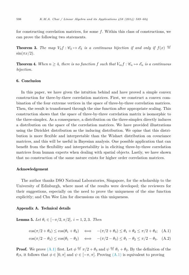
Lemma 5. Let θi ∈ [−π/2, π/2], i = 1, 2, 3. Then

cos(π/2 + θ3) ≤ cos(θ1 + θ2) ⇐⇒ −(π/2 + θ3) ≤ θ1 + θ2 ≤ π/2 + θ3; (A.1)

cos(π/2 − θ3) ≤ cos(θ1 − θ2) ⇐⇒ −(π/2 − θ3) ≤ θ1 − θ2 ≤ π/2 − θ3. (A.2)

Proof. We prove (A.1) first. Let φ def= π/2 + θ3 and ψ def= θ1 + θ2. By the definition of the θis, it follows that φ ∈ [0, π] and ψ ∈ [−π, π]. Proving (A.1) is equivalent to proving

K.M.A. Chai / Linear Algebra and its Applications 458 (2014) 589–604 599

Fig. 6. The cos(x) curve for x ∈ [−π, π]. The curve is strictly increasing in [−π, 0] and then strictly decreasing in [0, π]. Hence, clearly (A.3) holds.

cosφ ≤ cosψ ⇐⇒ −φ ≤ ψ ≤ φ. (A.3)

This can be shown by examining Fig. 6. The proof for (A.2) is similar, but using φ def= π/2 − θ3 and ψ def= θ1 − θ2 instead. �Lemma 6. Let ri ∈ [−1, 1] and θi

def= arcsin ri, for i = 1, 2, 3. Further, let

θ̃ def=

⎛⎜⎜⎝

θ1θ2θ3π/2

⎞⎟⎟⎠ ; A def=

⎛⎜⎜⎝

1 −1 −1 1−1 1 −1 1−1 −1 1 11 1 1 1

⎞⎟⎟⎠ .

Then the elements of the vector Aθ̃ are non-negative if and only if

|r3 − r1r2| ≤[(

1 − r21)(

1 − r22)]1/2

. (A.4)

Proof. First, we re-parameterise (A.4) using ri = sin θi, which is a bijection between the ris and the θis when ri ∈ [−1, 1]. Using the identity cos2 ψ + sin2 ψ = 1, we rewrite (A.4) as

| sin θ3 − sin θ1 sin θ2| ≤ cos θ1 cos θ2.

Removing the absolute function | ·|, rearranging, and then using the identity cos(φ ±ψ) =cosφ cosψ ∓ sinφ sinψ, gives

− cos(θ1 + θ2) ≤ sin θ3 ≤ cos(θ1 − θ2). (A.5)

By using the identity sinψ = cos(π/2 − ψ) on the sine term above, and then applying Lemma 5 (A.2) to the upper bound, we obtain

−(π/2 − θ3) ≤ θ1 − θ2 ≤ π/2 − θ3. (A.6)

Similarly, by using the identity sinψ = − cos(π/2 + ψ) on the sine term in (A.5), and then applying Lemma 5 (A.1) to the lower bound, we obtain

600 K.M.A. Chai / Linear Algebra and its Applications 458 (2014) 589–604

−(π/2 + θ3) ≤ θ1 + θ2 ≤ π/2 + θ3. (A.7)

There are four inequalities on θ1 ± θ2 in (A.6) and (A.7). These can be arranged as

θ1 − θ2 − θ3 + π/2 ≥ 0;

−θ1 + θ2 − θ3 + π/2 ≥ 0;

−θ1 − θ2 + θ3 + π/2 ≥ 0;

θ1 + θ2 + θ3 + π/2 ≥ 0. (A.8)

The left hand sides of these inequalities can be stacked and written as Aθ̃. Hence the elements of Aθ̃ must be non-negative to satisfy these four inequalities. �

To complete the proof for Theorem 1, we identify M = A/2.

Proof of Corollary 2. Let θi def= arcsin ri, i = 1, 2, 3. Using Theorem 1 and the change of variables formula gives

Pr(C) ≡ Pr(r) = Pr(θ)∣∣∣∣dθ

T

dr

∣∣∣∣ = Pr(α)∣∣∣∣dθ

T

dr

∣∣∣∣∣∣∣∣dα̃

T

dθ

∣∣∣∣,

where α = (α1, . . . , α4)T is as in Theorem 1(4); and α̃ def= (α1, α2, α3)T. The Jacobian for the first transformation is diagonal, with the ith diagonal entry

dθi/dri = dθi/d sin θi = 1/ cos θi,

so its determinant is the product of the reciprocals of the cos θis. For the second trans-formation, we let α4 = 1 − α1 − α2 − α3 so that α4 is completely determined by the vector α̃ of three random variables. Hence, the change of variables is via the mapping

α̃ = 12π

⎛⎝ 1 −1 −1

−1 1 −1−1 −1 1

⎞⎠ θ + 1

4

⎛⎝ 1

11

⎞⎠

obtained from (7). The volume of the Jacobian of this mapping is 1/2π3, so

Pr(C) = Pr(α)∣∣2π3 cos θ1 cos θ2 cos θ3

∣∣−1.

The proof is completed using the identity cos(arcsin x) = (1 − x2)1/2. �Lemma 7. Let λ1 ≥ λ2 ≥ λ3 be the eigenvalues of a three-by-three correlation matrix. Then the coordinate (λ1, λ2, λ3) is in the 2-simplex embedded within R3 with vertices (3, 0, 0), (1.5, 1.5, 0) and (1, 1, 1).

K.M.A. Chai / Linear Algebra and its Applications 458 (2014) 589–604 601

Proof. The characteristic polynomial of the correlation matrix is a depressed cubic equa-tion in (1 −λ) with roots (1 −λi), i = 1, 2, 3. The coefficient of the quadratic term in the equation is zero, so

∑3i=1(1 − λi) = 0 or, equivalently,

∑3i=1 λi = 3. Further applying

the inequality constraints λ1 ≥ λ2 ≥ λ3 ≥ 0 completes the proof. �We state four known results before proving Theorems 3 and 4.

Lemma 8. A continuous bijection from R to R must be strictly monotone.

Lemma 9. Vmf is bijective if and only if f is bijective.

Lemma 10. The correlation of an order n equicorrelation matrix is in [−1/(n − 1), 1].

Theorem 11. (See [5, Theorem 2.5].) En has 2n−1 extreme vertices, that is, |Vn| = 2n−1.

Let A def= (1, 1, 1), B def= (−1, −1, 1), C def= (−1, 1, −1), and D def= (1, −1, −1) denote the vertices in the tetrahedron C3. The following lemmas on C3 build towards Theorem 3.

Lemma 12. Consider a continuous bijection g : [−1, 1] �→ [−1, 1] where V3g : C3 �→ C3. Then g must be increasing with g(1) = 1 and g(−1) = −1.

Proof. Since g is a continuous bijection, it is monotone (Lemma 8), either increasing or decreasing. Also, it must be that g(1) = 1 or g(1) = −1. Since (−1, −1, −1) /∈ C3, it must be that V3g(A) = A. So g(1) = 1, and consequently g(−1) = −1, and g must be increasing. �Lemma 13. Under the setting in Lemma 12, let t ∈ [−1, 1] satisfies g(t) = t. Then g(1 + t − s) = 1 + t − g(s) for all s ∈ [t, 1].

Proof. Consider the two-dimensional slice in C3 where the third coordinate is t. This is a rectangle with four vertices (t, 1, t), (1, t, t), (−t, −1, t) and (−1, −t, t), which are on the lines AC, AD, BD and BC respectively; see Fig. 7. At t = 1 (resp. t = −1), this rectangle degenerates into the line AB (resp. CD).

If s ∈ [t, 1], then g(s) ≥ t because g is increasing (Lemma 12) and g(t) = t (the assumption). Consider a point (s, 1 + t − s, t) on the edge (t, 1, t) − (1, t, t) of the rect-angle. Applying V3g on this point gives point P def= (g(s), g(1 + t − s), t). Since the third coordinate is t, point P is on the same rectangle. Moreover, since the first coordinate g(s) ∈ [t, 1], we require g(1 + t − s) ≤ 1 + t − g(s) to keep P inside the rectangle.

We now show, by contradiction, that the equality must hold. Suppose g(1 + t − s) <1 + t − g(s). Then there must exist a point, say, (s, a, t), where a = 1 + t − s, such that g(a) = 1 +t −g(s) in order that V3g : C3 �→ C3 is a bijection. Since (s, 1 +t −s, t) is on the edge of the rectangle, it must be that a < 1 + t − s. Applying g to both sides retains the order of the inequality because g is strictly increasing, so g(a) < g(1 +t −s) < 1 +t −g(s),

602 K.M.A. Chai / Linear Algebra and its Applications 458 (2014) 589–604

Fig. 7. This figure illustrates the set of points considered in the proof of Lemma 13. The vertices of the tetra-hedron C3 are A = (1, 1, 1); B = (−1,−1, 1); C = (−1, 1,−1); and D = (1,−1,−1). The shaded rectangle made up of the trapezium and the triangle within C3 is where the third coordinate has constant value t. The shaded triangle is where the first coordinate s satisfies s ≥ t. The point represented by the filled circle is on an edge of the rectangle, and its second coordinate satisfies 1 + t − s. The proof demands that this point must stay on the same edge after the transformation V3g.

where the last inequality is the assumption within this paragraph. But this contradicts the requirement that g(a) = 1 +t −g(s). Hence it must be that g(1 +t −s) = 1 +t −g(s). �

By choosing suitable values for s and t, we obtain the following corollaries.

Corollary 14. Under the setting in Lemma 12, g is odd.

Proof. From Lemma 12, we use t = −1 in Lemma 13 to get g(−s) = −g(s) for all s ∈ [−1, 1]. �Corollary 15. Under the setting in Lemma 12, g(±(1 − 1/2n)) = ±(1 − 1/2n) for all n ∈ N.

Proof. From Corollary 14, g(0) = 0. For Lemma 13, we choose s = (1 + t)/2 to obtain g((1 + t)/2) = (1 + t)/2, and we repeatedly apply this starting from t = 0 to obtain g(1 − 1/2n) = 1 − 1/2n for all n ∈ N. Applying Corollary 14 completes the proof. �Lemma 16. Under the setting in Lemma 12, we have g(k/2n) = k/2n for all n ∈ N and k = −2n, −2n + 1, . . . , 2n − 1, 2n.

Proof. We proof by induction. Let n ∈ N. The base case k = −2n follows from Lemma 12. For the inductive step, assume g(k/2n) = k/2n for some k in {−2n, 2n + 1, . . . , 2n − 1}. Let t = k/2n and s = 1 − 1/2n. Then g(t) = t by the inductive hypothesis, and g(s) = s

by Corollary 15. We verify that s ∈ [t, 1] and apply Lemma 13 to give g((k + 1)/2n) =(k + 1)/2n. �Theorem 17. Under the setting in Lemma 12, g must be the identity function.

Proof. Let S be the set of dyadic rationals in [−1, 1]. This set is dense in [−1, 1] because the set of dyadic rationals is dense in R. Hence any c ∈ [−1, 1] is either in S or is a limit point in S. If the former, then Lemma 16 gives g(c) = c. Otherwise, let (xn)n∈N be the

K.M.A. Chai / Linear Algebra and its Applications 458 (2014) 589–604 603

sequence in S that converges to c. Applying Lemma 16 gives g(xn) = xn. By continuity of g, we have g(c) = limn→∞ g(xn) = limn→∞ xn = c. �Proof of Theorem 3. Let f(x) def= sin(πx/2). That V3f is a continuous bijection between C3 and E3 has essentially been shown by Theorem 1. Only uniqueness remains to be proved.

Suppose V3h, for some h : [−1, 1] �→ [−1, 1], is also a continuous bijection between C3 and E3. Then h = f ◦ f−1 ◦ h = f ◦ g is the same continuous bijection, where g def= f−1 ◦ h and g : C3 �→ C3. Since f−1 and h are continuous, g must be continuous. Using Theorem 17 gives h = f . �Proof of Theorem 4. First, we prove for n = 4 by contradiction. Let X, Y , Z and W be random variables. Then E4

def= {(rXY , rXZ , rY Z , rWX , rWY , rWZ)} is the space of their correlations. And the convex hull C4 is the space of the convex combination of the eight vectors (Theorem 11)⎛⎜⎜⎜⎜⎜⎜⎜⎝

1−1−1−1−11

⎞⎟⎟⎟⎟⎟⎟⎟⎠

,

⎛⎜⎜⎜⎜⎜⎜⎜⎝

1−1−111−1

⎞⎟⎟⎟⎟⎟⎟⎟⎠

,

⎛⎜⎜⎜⎜⎜⎜⎜⎝

−11−1−11−1

⎞⎟⎟⎟⎟⎟⎟⎟⎠

,

⎛⎜⎜⎜⎜⎜⎜⎜⎝

−11−11−11

⎞⎟⎟⎟⎟⎟⎟⎟⎠

,

⎛⎜⎜⎜⎜⎜⎜⎜⎝

−1−111−1−1

⎞⎟⎟⎟⎟⎟⎟⎟⎠

,

⎛⎜⎜⎜⎜⎜⎜⎜⎝

−1−11−111

⎞⎟⎟⎟⎟⎟⎟⎟⎠

,

⎛⎜⎜⎜⎜⎜⎜⎜⎝

111111

⎞⎟⎟⎟⎟⎟⎟⎟⎠

,

⎛⎜⎜⎜⎜⎜⎜⎜⎝

111−1−1−1

⎞⎟⎟⎟⎟⎟⎟⎟⎠

.

Let w1, . . . , w8 denote the above vectors, from left to right. These make up V4, the set of extreme vertices in E4.

Let [C4]3 (resp. [E4]3) be the volume in the first three dimensions of C4 (resp. E4). In the first three dimensions, vectors w2k−1 and w2k can be paired to the vector uk in V3(see Section 2.3), for k = 1, . . . , 4. For example, (w1 +w2)/2 gives u1. Hence [C4]3 ≡ C3. Similarly, [E4]3 ≡ E3. This can be shown when we let W be uncorrelated to the other variables so that the correlations between X, Y and Z are free to vary within E3.

Suppose function f is such that V6f : C4 �→ E4 is a continuous bijection. Then fand V3f : [C4]3 �→ [E4]3 are also continuous bijections (Lemma 9). Since [C4]3 ≡ C3 and [E4]3 ≡ E3, Theorem 3 says that f(x) must be sin(πx/2).

We now consider the point a in C4 that is the convex combination of w1, . . . , w8with mixture weights 1/3, 0, 1/3, 0, 1/3, 0, 0, 0; that is, a = −�1/3. Applying V6f with f(x) ≡ sin(πx/2) gives −�1/2. But −�1/2 /∈ E4 because −1/2 /∈ [−1/3, 1]; see Lemma 10. Therefore f is not a bijection, which contradicts our assumption. Hence, there is no function f such that V6f : C4 �→ E4 is a continuous bijection.

For n ≥ 5, let [Cn]6 (resp. [En]6) be the volume in the six dimensions of Cn (resp. En) that correspond to the correlations between four of the n random variables. Then [Cn]6 ≡ C4 and [En]6 ≡ E4, which can be shown using the same argument that [C4]3 ≡ C3and [E4]3 ≡ E3. But there is no continuous bijection V6f : C4 �→ E4. Hence there is no continuous bijection Vmf : Cn �→ En, where m = n(n− 1)/2. �

604 K.M.A. Chai / Linear Algebra and its Applications 458 (2014) 589–604

In the above proof, we have made use of the uniqueness of f , that is, f(x) =sin(πx/2). However, we really only need the uniqueness of f at x = −1/3, that is, f(−1/3) = −1/2. This can be shown by using Lemma 12 and then considering the point (−1/3, −1/3, −1/3) in C3.

References

[1] M. Arav, F.J. Hall, Z. Li, A Cauchy–Schwarz inequality for triples of vectors, Math. Inequal. Appl. 11 (2008) 629–634.

[2] W.J. Boscardin, X. Zhang, Modeling the covariance and correlation matrix of repeated measures, in: Applied Bayesian Modeling and Causal Inference from Incomplete-Data Perspectives, in: Wiley Series in Probability and Statistics, Wiley, 2004, pp. 215–226.

[3] J. Dattorro, Convex Optimization & Euclidean Distance Geometry, Meboo Publishing, Palo Alto, CA, USA, 2008.

[4] S.S. Gupta, Probability integrals of multivariate normal and multivariate t, Ann. Math. Statist. 34 (1963) 792–828.

[5] M. Laurent, S. Poljak, On a positive semidefinite relaxation of the cut polytope, Linear Algebra Appl. 223–224 (1995) 439–461.

[6] I. Olkin, Range restrictions for product-moment correlation matrices, Psychometrika 46 (1981) 469–472.

[7] S. Puntanen, G.P.H. Styan, Schur complements in statistics and probability, in: F. Zhang (Ed.), The Schur Complement and Its Applications, in: Numerical Methods and Algorithms, Springer, 2005, pp. 163–226.

[8] S. Puntanen, G.P.H. Styan, J. Isotalo, Matrix Tricks for Linear Statistical Models: Our Personal Top Twenty, Springer, 2011.

[9] P.J. Rousseeuw, G. Molenberghs, The shape of correlation matrices, Amer. Statist. 48 (1994) 276–279.