Reshetov LA Narrowband signal detection techniques in shallow ocean
Upload
independentCategory
view
1download
0
Narrowband and Wideband DOAEstimation with Unknown Number
of Sources
Vinod Veera Reddy
School of Electrical and Electronic Engineering
A thesis submitted to Nanyang Technological University
in partial fulfillment of the requirement for the degree of
Doctor of Philosophy
2013
Acknowledgments
Firtstly, I would like to express my gratitude to my supervisors, Prof. Andy Khong andProf. Ng Boon Poh, for their continuous encouragement, guidance and support with thefollowing prayer:
(My teachers are the Gods, Brahma, Vishnu and Shiva.They are the form of abolute truth. I bow to them with gratitude.)
I am grateful to my ex-supervisor Prof. Farook Sattar, friends Anil, Vishwa andmy parents who inspired me to pursue with my PhD studies. Their moral support andblessings have been the main source of fuel in this journey.
I would also like to thank my seismic, statina and array processing team memberswith whom I felt very comfortable to have technical discussions and immensely enjoyedthe techshare sessions. My ex-teammates and friends, Joni, Aye Aung, Ajay, Divya,Zhang Ying, Wen Fuxi, Santosh, Jayachandra, Aishwarya. V and Chitra have greatlyhelped me in the due course of this study. I would like to acknowledge the support ofISR lab technicians, Mr. Mui Eng Teck and Ms. Hoay-Lim Suat Geok.
Special thanks to my family members Tanuja, Sunil, JaiKumar, Meghana and my wifeDharaNi for their warm love and encouragement. I have cherished the last three yearsbeing a part of Nikam Guruji Yoga Kutir which conducts yoga classes across Singapore.
Finally, I would like to dedicate this thesis to my parents.
i
Abstract
Array processing has been an active research area for several decades. The advent of newsignal processing techniques has maintained this topic afresh in the research communitywith new challenging problems. The estimation of direction-of-arrival (DOA) for instancehas evolved from high-resolution to superresolution techniques, and of-late, is headingtowards increasing the available degrees of freedom. Excited by these developments andthe awaiting potential applications, we have considered the study of DOA estimation fornarrowband and wideband sources in this thesis under various conditions.
Within an array processing system, the inter-dependence between the model-orderestimation, DOA estimation and beamforming tasks reflects the sensitivity of one taskto the outcome of the other. In view of this, beamformers have been designed in the pastto incorporate robustness against look direction mismatch and array manifold errors.However, existing DOA estimation techniques are sensitive to the accuracy of estimatednumber of sources. In order to overcome this limitation, we propose a new narrow-band DOA estimation technique which substitutes the noise subspace eigenvectors witha weight vector matrix. This allows one to obtain the spatial spectrum with unknownnumber of sources. Any error in model order estimation will therefore have no impacton the accuracy of DOA estimates.
Estimating the number of sources in the presence of wideband sources is a very chal-lenging task considering the fact that existing techniques retrieve the model order eitherfrom a coherently-averaged covariance matrix or by the maximum likelihood approach.While the estimated model-order from the former method is susceptible to the initialestimates, the latter technique is computationally expensive. We therefore present atime-domain DOA estimation technique which provides distinct peaks along the sourcedirections in its spatial spectrum without estimating the number of sources. The un-derlying idea relies on the array manifold approximation using Taylor series expansionacross the signal bandwidth. The undesired derivative components are then suppressedby the proposed optimization problem. The effectiveness of this technique is verified witha detailed mathematical analysis and simulations.
With finite-ordered Taylor series expansion, the array manifold approximation is accu-rate for sources with a percentage bandwidth less than 30%. For larger source bandwidth,the estimation accuracy of the time-domain technique decreases. We therefore transformthe problem to frequency domain and perform DOA estimation on a regulated signalbandwidth.
ii
Environmental factors such as multipath, dispersion and scattering adversely affectthe performance of existing DOA estimation techniques in many applications such asradio wave communication, seismic and underwater acoustic applications. Existing tech-niques such as matched-field processing incorporate the speed profile and introduce ro-bustness to random perturbations in speed. However, the estimation of speed profileis itself challenging and inaccurate many times. We therefore consider redefining arraymanifold approximation such that robustness can be incorporated to dispersion. Theoptimization problem introduces derivative compensation with respect to the wavenum-ber which absorbs the effect of dispersion in the signal model. With this approach, onerequires to only estimate the propagation speed at only a reference frequency instead ofthe entire source bandwidth.
iii

Contents
Acknowledgments . . . . . . . . . . . . . . . . . . . . . . . . . . . . . . . . . . i
Abstract . . . . . . . . . . . . . . . . . . . . . . . . . . . . . . . . . . . . . . . . ii
List of Figures . . . . . . . . . . . . . . . . . . . . . . . . . . . . . . . . . . . . vii
List of Acronyms . . . . . . . . . . . . . . . . . . . . . . . . . . . . . . . . . . xii
List of Notations . . . . . . . . . . . . . . . . . . . . . . . . . . . . . . . . . . . xiii
1 Introduction 1
1.1 Background . . . . . . . . . . . . . . . . . . . . . . . . . . . . . . . . . . 1
1.2 Narrowband vs Wideband Signals . . . . . . . . . . . . . . . . . . . . . . 3
1.3 Motivation and Objectives . . . . . . . . . . . . . . . . . . . . . . . . . . 5
1.4 Contributions of this Thesis . . . . . . . . . . . . . . . . . . . . . . . . . 7
1.5 Statement of Originality and Publications Related to this Thesis . . . . . 9
2 Fundamentals of Array Processing 11
2.1 Wave Propagation and Spatial Sampling . . . . . . . . . . . . . . . . . . 11
2.2 Narrowband Array Processing . . . . . . . . . . . . . . . . . . . . . . . . 15
2.2.1 Beamforming . . . . . . . . . . . . . . . . . . . . . . . . . . . . . 15
2.2.2 DOA Estimation . . . . . . . . . . . . . . . . . . . . . . . . . . . 18
2.2.3 Model-Order Estimation . . . . . . . . . . . . . . . . . . . . . . . 22
2.3 Wideband Array Processing . . . . . . . . . . . . . . . . . . . . . . . . . 23
2.3.1 Beamforming . . . . . . . . . . . . . . . . . . . . . . . . . . . . . 26
2.3.2 DOA Estimation . . . . . . . . . . . . . . . . . . . . . . . . . . . 29
2.3.3 Model-Order Estimation . . . . . . . . . . . . . . . . . . . . . . . 38
iv

3 Narrowband DOA Estimation without Order Selection 41
3.1 Introduction . . . . . . . . . . . . . . . . . . . . . . . . . . . . . . . . . . 41
3.2 MUSIC-like Narrowband DOA Estimator . . . . . . . . . . . . . . . . . . 42
3.2.1 Formulation . . . . . . . . . . . . . . . . . . . . . . . . . . . . . . 42
3.2.2 Detailed Analysis . . . . . . . . . . . . . . . . . . . . . . . . . . . 44
3.2.3 Bounds for β . . . . . . . . . . . . . . . . . . . . . . . . . . . . . 50
3.3 Proposed DOA Estimation Technique (MUSIC-W) . . . . . . . . . . . . 52
3.3.1 Computational Complexity . . . . . . . . . . . . . . . . . . . . . . 57
3.4 Simulation Results . . . . . . . . . . . . . . . . . . . . . . . . . . . . . . 58
3.5 Conclusion . . . . . . . . . . . . . . . . . . . . . . . . . . . . . . . . . . . 64
4 Time-Domain Wideband DOA Estimation 67
4.1 Introduction . . . . . . . . . . . . . . . . . . . . . . . . . . . . . . . . . . 67
4.2 Array Manifold Approximation for Wideband Signal Model . . . . . . . . 69
4.3 Proposed Technique . . . . . . . . . . . . . . . . . . . . . . . . . . . . . . 72
4.3.1 Formulation . . . . . . . . . . . . . . . . . . . . . . . . . . . . . . 73
4.3.2 Discussion . . . . . . . . . . . . . . . . . . . . . . . . . . . . . . . 75
4.3.3 Computational Complexity . . . . . . . . . . . . . . . . . . . . . . 79
4.3.4 The {f, φ} Ambiguity . . . . . . . . . . . . . . . . . . . . . . . . 81
4.4 Derivation of the Cramer-Rao Lower Bound (CRLB) . . . . . . . . . . . 84
4.5 Simulation Results and Discussions . . . . . . . . . . . . . . . . . . . . . 86
4.6 Conclusion . . . . . . . . . . . . . . . . . . . . . . . . . . . . . . . . . . . 94
5 Derivative-Constrained Frequency-Domain Wideband DOA Estimation100
5.1 Introduction . . . . . . . . . . . . . . . . . . . . . . . . . . . . . . . . . . 100
5.2 Signal Model with Array Manifold Approximation . . . . . . . . . . . . . 105
5.3 Proposed DOA Estimation . . . . . . . . . . . . . . . . . . . . . . . . . . 108
5.3.1 Frequency-Averaged BFW-MUSIC Formulation (Formulation 1) . 109
5.3.2 Frequency-Averaged Wideband MUSIC-like Algorithm (Formula-
tion 2) . . . . . . . . . . . . . . . . . . . . . . . . . . . . . . . . . 111
5.3.3 Multiband DOA Estimation (Formulation 3) . . . . . . . . . . . . 112
5.4 Simulation Results . . . . . . . . . . . . . . . . . . . . . . . . . . . . . . 113
v

5.4.1 Simulation Setup and Illustrations . . . . . . . . . . . . . . . . . . 113
5.4.2 Performance Evaluation . . . . . . . . . . . . . . . . . . . . . . . 118
5.5 Discussions and Concluding Remarks . . . . . . . . . . . . . . . . . . . . 122
6 Wideband DOA Estimation in Dispersive Medium 126
6.1 Introduction . . . . . . . . . . . . . . . . . . . . . . . . . . . . . . . . . . 126
6.2 Signal Model . . . . . . . . . . . . . . . . . . . . . . . . . . . . . . . . . 129
6.3 Array Manifold Approximation . . . . . . . . . . . . . . . . . . . . . . . 132
6.4 Proposed Technique . . . . . . . . . . . . . . . . . . . . . . . . . . . . . . 134
6.5 Simulation Results and Discussions . . . . . . . . . . . . . . . . . . . . . 136
6.6 Conclusion . . . . . . . . . . . . . . . . . . . . . . . . . . . . . . . . . . . 141
7 Conclusion and Future Directions 142
7.1 Conclusion . . . . . . . . . . . . . . . . . . . . . . . . . . . . . . . . . . . 142
7.2 Future Directions . . . . . . . . . . . . . . . . . . . . . . . . . . . . . . . 145
Author’s Publications 148
References 150
vi
List of Figures
1.1 Relation between the three major problems observed in array processing. 4
2.1 Illustration of an L-sensor ULA sampling a plane wave from direction θ. 13
2.2 A typical narrowband beamformer with complex weights. . . . . . . . . . 16
2.3 Source spectrum, (a) bandpass signal, (b) band-limited signal. . . . . . . 24
2.4 Wideband array processing in time-domain, (a) block diagram, (b) using
FIR filters with pre-steering. . . . . . . . . . . . . . . . . . . . . . . . . . 40
3.1 Steered response power of MVDR and the algorithm under consideration
obtained from the cost function of (3.1) for L = 5 and M = 2; R generated
using 100 snapshots. . . . . . . . . . . . . . . . . . . . . . . . . . . . . . 46
3.2 Spatial spectrum of MUSIC and MUSIC-like algorithms for L = 5 sensors
with synthetic covariance matrix generated using (2.20). . . . . . . . . . 48
3.3 Spatial spectrum of MUSIC and MUSIC-like algorithms with 100 snap-
shots for L = 5,M = 2 and SNR=5 dB. . . . . . . . . . . . . . . . . . . . 49
3.4 Generalized eigenvalue χmin corresponding to the solution weight vector
plotted against the scan direction for L = 5,M = 2 with 100 snapshots
and SNR=5 dB. . . . . . . . . . . . . . . . . . . . . . . . . . . . . . . . . 54
3.5 Spatial spectrum of MUSIC-W algorithm in comparison with that of MU-
SIC and MUSIC-like algorithms at SNR=5 dB. . . . . . . . . . . . . . . 56
3.6 Spatial spectrum of MUSIC-W with W constructed with weight vectors
obtained at SNR=5 dB from the azimuth range (a) 10◦ to 90◦, (b) 90◦ to
170◦. K = L weight vectors are used in W. . . . . . . . . . . . . . . . . 57
3.7 RMSE of source estimates using the MUSIC-like algorithm plotted against
η at various SNR values. . . . . . . . . . . . . . . . . . . . . . . . . . . . 59
vii

3.8 RMSE of source estimates obtained with the MUSIC-W algorithm plotted
against K at various SNR values. . . . . . . . . . . . . . . . . . . . . . . 60
3.9 RMSE of source estimates plotted against SNR for the MUSIC-like, MUSIC-
W, MVDR and MUSIC algorithms. . . . . . . . . . . . . . . . . . . . . . 61
3.10 The probability of resolving two closely situated sources with 100 snapshots. 63
3.11 The RMSE of source estimates plotted against snapshots for the MUSIC-
like, MUSIC-W, MUSIC and MVDR algorithms. . . . . . . . . . . . . . . 66
4.1 Plot of aH(f0,φ)(R+ζRy(φ))−1a(f0,φ)
χ(R+ζRy(φ))−1,maxand aH(f0,φ)R−1a(f0,φ)
χR−1,maxin the presence of
three sources. . . . . . . . . . . . . . . . . . . . . . . . . . . . . . . . . . 79
4.2 Illustrative spatial spectrum of the proposed technique. . . . . . . . . . . 80
4.3 Performance of the proposed technique under the {f, φ} ambiguity at an
SNR of 5 dB (a) without time delay taps, (b) with D = 3 time delay taps. 83
4.4 Ten-element double ring circular array. . . . . . . . . . . . . . . . . . . . 87
4.5 Spatial spectra with different derivative orders P at an SNR of 5 dB for
(a) BFW-MUSIC, (b) proposed technique. . . . . . . . . . . . . . . . . . 88
4.6 RMSE of the DOA estimates plotted for various SNR values against (a)
η, (b) ζ. . . . . . . . . . . . . . . . . . . . . . . . . . . . . . . . . . . . . 89
4.7 RMSE of DOA estimates against SNR with 1500 time-domain snapshots. 95
4.8 RMSE of DOA estimates as a function of the number of snapshots in
comparison with the BFW-MUSIC algorithm. The snapshots are obtained
at 5 dB SNR. . . . . . . . . . . . . . . . . . . . . . . . . . . . . . . . . . 96
4.9 Probability of resolving two sources with angular separations ∆θ = 5◦,
∆θ = 7◦ and ∆θ = 9◦. . . . . . . . . . . . . . . . . . . . . . . . . . . . . 97
4.10 RMSE of DOA estimates against SNR in comparison with the CSSM,
TOPS and BFW-MUSIC algorithms when the sources are situated at 12◦,
40◦ and 48◦. . . . . . . . . . . . . . . . . . . . . . . . . . . . . . . . . . . 98
4.11 The probability of resolving all the three sources by CSSM, TOPS, BFW-
MUSIC and the proposed technique. . . . . . . . . . . . . . . . . . . . . 99
5.1 Error in steering vector approximation using TSE against (a) derivative
order for δf = 0.04, (b) δf for various values of P . . . . . . . . . . . . . . 102
viii
5.2 RMSE of DOA estimates plotted against fractional bandwidth. . . . . . . 103
5.3 Performance of MDL and AIC techniques against SNR when J = 10
frequency-domain snapshots are used. . . . . . . . . . . . . . . . . . . . . 104
5.4 Spatial spectrum obtained for the proposed formulations. . . . . . . . . . 115
5.5 Spatial spectrum for various signal subspace dimensions of Rav. . . . . . 116
5.6 Spatial spectrum obtained for the two proposed formulations. Sources
located at 40◦ and 48◦ are completely correlated. . . . . . . . . . . . . . . 117
5.7 DOA estimation performance against fractional bandwidth being processed:
(a) probability of resolving the closely-situated sources, (b) RMSE of es-
timates averaged over the three sources. . . . . . . . . . . . . . . . . . . 119
5.8 The RMSE of DOA estimates for CSSM, TD-DOA and the proposed
frequency-domain formulations plotted against SNR. . . . . . . . . . . . 123
5.9 The probability of resolving all the three sources plotted against SNR for
various formulations. . . . . . . . . . . . . . . . . . . . . . . . . . . . . . 124
5.10 The plot of RMSE for the second source direction estimate using Formu-
lation 2 for various processing bandwidths. . . . . . . . . . . . . . . . . . 124
5.11 The RMSE of DOA estimates plotted against the number of frequency-
domain snapshots used. . . . . . . . . . . . . . . . . . . . . . . . . . . . . 125
6.1 (a) Dispersion function with the propagation speed plotted against fre-
quency for γ = −60 and γ = 60. (b) Spatial spectrum obtained by the
proposed technique for the two values of γ with SNR set to 5 dB. . . . . 138
6.2 Estimation performance of the proposed technique plotted against the non-
linearity function parameters, (a) γ, (b) ∆νmax. . . . . . . . . . . . . . . 139
6.3 (a) Estimation performance of the proposed technique plotted against SNR
for, (a) Source 1, (b) Source 2. . . . . . . . . . . . . . . . . . . . . . . . . 140
6.4 (a) Dispersion function with the propagation speed obtained using (6.26)plotted
against frequency. (b) Spatial spectrum obtained by the proposed tech-
nique and the STCM-MVDR algorithm at an SNR of 0 dB. . . . . . . . 141
ix

Acronyms
MVDR Minimum Variance Distortionless ResponseEVD EigenValue DecompositionSVD Singular Value DecompositionMUSIC MUltiple SIgnal ClassificationESPRIT Estimation of Signal Parameters via Rotational Invariance TechniqueFIB Frequency Invariant BeamformingISSM Incoherent Signal Subspace MethodCSSM Coherent Signal Subspace MethodTOPS Test for Orthogonality of Projection SubspacesBFW-MUSIC Beamforming Framework Wideband MUSICSTCM STeered Covariance MatrixGEV Generalized EigenValueULA Uniform Linear ArraySNR Signal-to-Noise RatioRMSE Root Mean Squared ErrorPHAT PHAse TransformGSCT Generalized State Coherence TransformKDE Kernel Density EstimatorSTCM-MVDR-MS Multi-Stage STCM-MVDRNTVE Normalized Time difference Vector Error
xii

xii

List of Notations
Chapters 1 and 2
∆f Fractional bandwidth of a wideband sourceθ Source directionφ Arbitrary look directionL Number of sensorsM Number of sourcesF Number of DFT/FFT pointsN Number of snapshotsa(θ) Steering vector in the direction θ for a narrowband signalx(n) Vector of sensor array snapshots(n) Vector of sourcesv(n) Vector of additive noiseA(Θ) Array manifold matrix with steering vectors forming its columnsPxx(f) Spectral density matrix of x(f)Pss(f) Spectral density matrix of s(f)Pvv(f) Spectral density matrix of v(f)R Array covariance matrixRss Source covariance matrixRvv Noise covariance matrixw Weight vector of a beamformerUs Matrix with signal subspace eigenvectorsUn Matrix with noise subspace eigenvectorsΛs Diagonal matrix with signal subspace eigenvaluesΛn Diagonal matrix with noise subspace eigenvaluesσ2v Noise powerJ Number of frequency domain snapshotsD Temporal delays used in the time-delay linex(f) Frequency domain sensor snapshota(fk, θ) Steering vector in the direction θ for a wideband signal at frequency fkx(n) Spatio-temporal sensor snapshotT(fk, φ) Transformation matrix. Focussing matrix in the context of CSSM.R(fk) Array covariance matrix at frequency fkRcssm Focussed covariance matrix employed in CSSMRfib Frequency invariant covariance matrix employed in FIB based DOA estimationR(φ) Steered covariance matrix used in STCM-MVDR
xiii

Chapter 3
wφ Weight vector evaluated at each look direction φPaφ Projection matrix of steering vector a(φ)χ Lagrangian parameterχmin Minimum eigenvalue of a generalized eigenvalue problemχA,min Minimum eigenvalue of matrix Atr{.} Trace of a matrixW Matrix formed with weight vectors from different directionsR{A} Range space of matrix AΛs Λs − σ2
vIL.
Chapter 4
δf Frequency deviation f − f0
P Order of derivative termsdp(f0, θ) pth derivative of the steering vector a(f0, θ) w.r.t. frequencyDp(θ) pth derivative of the array manifold matrix A(f0,Θ) w.r.t. frequencyDf0,φ Derivative matrix with 1 : P order derivative vectors from look direction φPDφ
Projection matrix of Df0,φ
a(f0, φ) Spatio-temporal steering vectorDf0,φ Derivative matrix with 1 : P order derivative vectors of a(f0, φ)R{.} Real part of the componentRy(φ) Covariance matrix of data projected onto the derivative vector space using Df0,φ
Chapter 5
B Number of frequency bins usedX(k) Data matrix at a frequency fkX Data matrix constructed over B frequency binsRav Average covariance matrix estimated over B frequency binsQ Number of subbandsEd Extended signal subspace matrix of Rav
Chapter 6
νp Phase velocityνg Group velocityκf frequency dependent wavenumbera(κf , φ) Steering vector from look direction φ
0.4pt0.1pt
xiv

Chapter 1
Introduction
1.1 Background
Any physical process can be transduced into an electrical signal using a sensor which
is then processed to extract necessary information. If multiple sensors are employed to
capture a signal, additional information about the physical phenomenon can be extracted.
The stream of signal processing which studies the unified treatment of signals acquired
from an array of sensors is widely known as Sensor Array Signal Processing. The wide
range of potential applications has kept array processing as an active area of research over
the last three decades. The concepts, problems and solutions have been well explained
in several books [1–4] and review articles [5, 6]. A few applications where sensor arrays
are used are listed below [2]:
(i) RADAR - RAdio Detection And Ranging is one of the well-known applications
employing array signal processing. The use of antenna array over a single antenna
enhances target detection rate as well as estimation of target range and speed.
Thanks to array processing and adaptive filter theory, moving objects can be con-
veniently tracked from the received signals. MIMO-RADAR has gained recent
1

Chapter 1. Introduction
interest of the research community due to its pertinence in commercial and defense
related applications.
(ii) SONAR - SOund Navigation And Ranging extends the application of RADAR to
acoustic signals underwater. With the medium uncertainties posing complicated
challenges, the use of sensor array aids in improving the system performance.
(iii) Communications - The seemless use of wireless communication for several ap-
plications increases the demand for bandwidth. Besides the conventional use of
sensor arrays for signal enhancement and interference suppression, arrays are used
to increase the channel capacity as well.
(iv) Seismology - The area of reflection seismology applicable for seismic exploration
uses geophone arrays to record reflections of a seismic event which can subsequently
be used to construct subsurface images. Geophone arrays can also be used to detect
and localize underground seismic events.
(v) Speech processing - Microphone arrays are gaining popularity in order to enhance
the quality of recorded speech by denoising and dereverberation. DOA estimation
and blind speech/audio source separation have been another applications where the
use of microphone array is advantageous.
Several other applications including the field of medical diagnosis (EEG, ECG, tomog-
raphy) and radio astronomy also use sensor arrays. This explains the need for such an
intensive research interest in the area of array signal processing. Several signal process-
ing algorithms have been developed to tackle problems specific to applications. Among
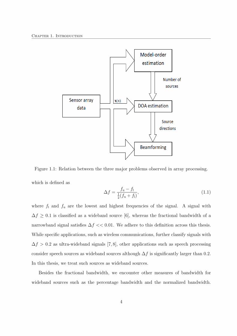
them, three widely observed problems are:
• Signal detection - The detection of all sources present in the scenario is the foremost
task to be performed with the acquired signal. In RADAR and SONAR applica-
2

Chapter 1. Introduction
tions, the detection of targets is a very critical task which is followed by parameter
estimation. Other tasks such as DOA estimation and beamforming are directly or
indirectly sensitive to the accurate estimation of the number of sources. Since the
order of the signal model signifies the number of sources present, this problem is
also termed as model order estimation. Most common approach for signal detection
is by formulating a multiple hypothesis test.
• Direction-of-Arrival (DOA) estimation - Once the sources present in a scenario are
detected, additional information from the array outputs need to be extracted. The
source directions are also preserved in the array outputs due to the spatial sepa-
ration of array elements. This permits the signal model to be parameterized with
source directions. The DOA estimates may serve as a prerequisite for beamforming.
• Beamforming - Constructive combination of signals across the sensors to recover
the signal is termed as beamforming, since the signal processor digitally focusses
a beam towards the direction of interest by providing appropriate weights to the
sensor outputs. Advanced design of the weights include constraints for interference
suppression and provide robustness to array manifold errors. Evidently, a DOA
estimation module may be followed by a beamformer in an array processing system.
The sequence and inter-relation between the three tasks are shown in Figure 1.1.
1.2 Narrowband vs Wideband Signals
The system design in any application, beginning from the choice of sensors to the front-
end design and the digital architecture, rely on the signal characteristics. A signal is first
classified as either narrowband or wideband in nature observing its fractional bandwidth
3
Chapter 1. Introduction
Figure 1.1: Relation between the three major problems observed in array processing.
which is defined as
∆f =fu − fl
12(fu + fl)
, (1.1)
where fl and fu are the lowest and highest frequencies of the signal. A signal with
∆f ≥ 0.1 is classified as a wideband source [6], whereas the fractional bandwidth of a
narrowband signal satisfies ∆f << 0.01. We adhere to this definition across this thesis.
While specific applications, such as wireless communications, further classify signals with
∆f > 0.2 as ultra-wideband signals [7, 8], other applications such as speech processing
consider speech sources as wideband sources although ∆f is significantly larger than 0.2.
In this thesis, we treat such sources as wideband sources.
Besides the fractional bandwidth, we encounter other measures of bandwidth for
wideband sources such as the percentage bandwidth and the normalized bandwidth.
4

Chapter 1. Introduction
Percentage bandwidth of a wideband source is the fractional bandwidth expressed as a
percentage, i.e., ∆f × 100%. The normalized bandwidth of a source is defined as the
bandwidth measured by normalizing all the frequencies w.r.t. the sampling frequency fs
and is evaluated as (fu − fl)/fs.
1.3 Motivation and Objectives
As observed from Figure 1.1, the three array processing modules are very closely re-
lated. The state-of-the-art narrowband DOA estimation techniques such as multiple sig-
nal classification (MUSIC) and estimation of signal parameters via rotational invariance
techniques (ESPRIT) provide good estimates with high resolution assuming accurate
knowledge of the number of sources present. Existing beamforming techniques rely sig-
nificantly on the source directions provided by the DOA estimation techniques. While
robust beamformers are designed to handle errors in source directions and array geom-
etry, existing DOA estimation techniques are observed to be susceptible to model-order
estimation errors.
Under very low signal-to-noise (SNR) conditions, or when the number of sensor snap-
shots are limited, model-order estimation techniques are more likely to identify incorrect
number of sources [9]. Although existing narrowband DOA estimation techniques can
estimate source directions under such adverse conditions, providing inaccurate number
of sources to these techniques results in incorrect DOA estimates. The model-order
estimation error propagates through various stages resulting in degradation of system
performance. This often translates to the need for DOA estimation techniques which are
robust towards model order estimation errors. One approach is to resort to beamforming
techniques which identify source directions from the steered response peaks. However,
obtaining the resolution of subspace-based techniques is challenging with this approach.
5

Chapter 1. Introduction
Towards this, a narrowband DOA estimation technique was recently proposed in [9]
which evaluates the spatial spectrum independent of the estimated model order. With
the beamforming framework, the performance of this technique was shown to approach
that of the MUSIC algorithm. However, the precise operation of the underlying opti-
mization problem has not been analyzed in detail. One of the main objectives of this
thesis is to provide a proper mathematical treatment to this algorithm. In this study, we
also justify that the technique is indeed a “MUSIC-like” algorithm with its performance
converging asymptotically to the MUSIC algorithm. This technique has limited perfor-
mance at a larger computational cost relative to the MUSIC algorithm. We therefore
aim to overcome these limitations with a modified approach.
A similar problem of incorrect model order estimation adversely affecting the DOA
estimation task is encountered for wideband sources. While the maximum likelihood
approach is computationally expensive, model-order estimation on coherently averaged
covariance matrix across the signal bandwidth is susceptible to focussing errors. It is
therefore essential to have a DOA estimation technique which is insensitive to the esti-
mated model order. Noting the advantages of the MUSIC-like algorithm proposed for
narrowband case earlier, it is imperative to formulate a wideband DOA estimation tech-
nique which does not rely on model-order estimation. This forms our second objective.
Radio wave propagation in the earth’s atmosphere is subject to many influences such
as refraction, reflection, diffraction, fading and scattering. The change in medium due
to atmospheric precipitation is known to attenuate signals beyond 10 GHz due to scat-
tering [10]. With rain drops accounting for the maximum attenuation, it is modeled as
a function of rain-rate which defines the density of rain drops. Besides this attenuation,
water particles ordain as a refractive medium which introduces dispersion. Dispersion is
a phenomenon in which the propagation speed changes with the signal frequency. Due
to the varying density of clouds and rain, attenuation and dispersion changes with time.
6
Chapter 1. Introduction
It is therefore difficult to precisely model these factors and compensate the same. Impre-
cise knowledge of the propagation speed variations adversely affects the performance of
existing wideband DOA estimation techniques. This emphasizes the need for introducing
robustness against dispersion in wideband DOA estimation. Addressing this problem can
aid in improving source localization performance in other applications such as seismic
and underwater acoustic applications. This serves as a motivation for us to develop a
wideband DOA estimation technique for dispersive medium which is robust to changes
in speed with frequency.
1.4 Contributions of this Thesis
Our first contribution is dedicated to the mathematical analysis of a recently proposed
narrowband DOA estimation technique [9] which is insensitive to the estimated model
order. Designed with a beamforming framework, the performance of this technique is
shown to approach that of the multiple signal classification (MUSIC) algorithm. We
perform a detailed analysis of the optimization problem which exhibits the prime differ-
ence between this technique with the minimum variance distortionless response (MVDR)
algorithm and show that it degenerates to the MUSIC algorithm asymptotically. We
then rederive the bounds for the sole parameter from the solution under the desired spa-
tial spectrum conditions. From the working principle of this algorithm, we identify a
new criteria for DOA estimation which outperforms the technique proposed in [9] and
approaches the performance of the MUSIC algorithm. The reduced computational cost
proves the proposed technique to be more appealing over that proposed in [9].
In the second contribution we propose a wideband DOA estimation technique which is
insensitive to errors in the estimated model order. For wideband sources with fractional
bandwidth up to 30%, the steering vector across the bandwidth can be approximated
7

Chapter 1. Introduction
using Taylor series expansion w.r.t. the frequency deviation from a reference frequency.
Employing Parseval’s relation, we deduce an approximated time-domain signal model
for wideband sources. The MUSIC-like algorithm studied in the previous contribution
is then extended for wideband DOA estimation by incorporating a quadratic derivative
term which reduces the problem to a narrowband problem. Besides the ability to estimate
source directions with variable bandwidth, this time-domain technique requires reduced
number of snapshots for DOA estimation.
The time-domain wideband DOA estimation technique relies on the validity of Tay-
lor series approximation of array manifold across the signal bandwidth. With the order
of Taylor series fixed due to design considerations, the array manifold approximation
error increases with the source bandwidth which, as a consequence, causes a reduction
in DOA estimation accuracy. We therefore maintain the manifold approximation in the
frequency domain and construct a covariance matrix with regulated signal bandwidth
within which the Taylor series approximation introduces minimum error. The resul-
tant derivative-constrained frequency domain wideband DOA estimation technique then
forms our third contribution. In order to exploit the DOA information across the entire
signal bandwidth, we present a multi-band DOA estimation approach which improves
the estimation accuracy.
In our fourth contribution, we consider wideband DOA estimation for an application
scenario in which the signals propagate through dispersive medium. The introduced
amount of dispersion is often an unknown function of rain-rate or cloud density. If
we model the change in the propagation speed as an unknown nonlinear function of
frequency, existing wideband DOA estimation techniques suffer from poor performance.
We therefore propose a technique with derivative constraints w.r.t. the wavenumber.
This technique introduces robustness to changes in the propagation speed across the
signal bandwidth and can be extended to seismic and underwater acoustic applications
8

Chapter 1. Introduction
when the dispersion profile is a continuous function of frequency.
The organization of this thesis is as follows: Chapter 2 provides the necessary back-
ground with the fundamentals of array processing. In Chapter 3, we present detailed
analysis of the MUSIC-like algorithm and propose a new narrowband DOA estimation
technique. Chapter 4 presents a new time-domain wideband DOA estimation technique
which does not rely on model-order estimation. In Chapter 5, we propose a frequency-
domain DOA estimation algorithm employing derivative constraints. Wideband estima-
tion in dispersive medium is then presented in Chapter 6. Chapter 7 follows with the
solution provided for unambiguous DOA estimation of speech sources under reverberant
environment. Chapter 8 concludes the thesis with possible future directions.
1.5 Statement of Originality and Publications Re-
lated to this Thesis
To the extent of the author’s knowledge, the following contributions of this thesis are
original:
(i) The detailed mathematical analysis of the MUSIC-like algorithm and the derivation
of bounds for its parameter presented in Chapter 3. This work has been submitted
for publication [J4].
(ii) The array manifold approximation using Taylor series and the time-domain wide-
band DOA estimation technique presented in Chapter 4. The publication related
to this work is [J1].
(iii) The derivative-constrained wideband DOA estimation discussed in Chapter 5 has
been accepted for publication [J2].
9

Chapter 1. Introduction
(iv) DOA estimation applicable for dispersive medium as discussed in Chapter 6 based
on Taylor series expansion w.r.t. the wavenumber. The manuscript is under prepa-
ration.
10

Chapter 2
Fundamentals of Array Processing
This chapter provides the necessary prerequisites to array signal processing for under-
standing and appreciating the subsequent chapters. The chapter starts with the study of
wave propagation and its sampling in the spatial domain. Defining a signal model for the
acquired narrowband signals first, we study the process of beamforming. We then review
a few subspace-based narrowband DOA estimation techniques and examine theproblem
of model-order estimation using hypothesis testing. The discussion transits to wideband
source scenario under which we discuss the tasks of beamforming, DOA estimation and
model-order estimation. The study of wideband DOA estimation is performed in detail
as it serves as a review of existing techniques required for subsequent chapters.
2.1 Wave Propagation and Spatial Sampling
Consider a wave propagating in a homogeneous lossless medium. The wave equation in
rectangular coordinates is then given by [11]
∇2s(t, r)− 1
ν2
∂2
∂t2s(t, r) = 0, (2.1)
11

Chapter 2. Fundamentals of Array Processing
where
∇2 =∂2
∂x2+
∂2
∂y2+
∂2
∂z2
is the Laplacian operator expressed in the Cartesian coordinates (x,y,z), s(t, r) is the
signal at time t and r is the spatial position in the medium and ν is the wave propagation
speed. Equation (2.1) is termed as the homogeneous wave equation since the left hand
side of the equation is equal to zero indicating that there is no external force or input
acting at r.
Defining A as the amplitude and f as the frequency of a complex sinusoidal signal
s(t) = A exp(2πft) (2.2)
propagating at a spatial point r in the medium, the solution to the wave equation leads
to the plane wave:
s(t, r) = s(t−α.r),
= A exp(2πf(t−α.r)) = A exp((ωt− κ.r)
) (2.3)
where α = (αx, αy, αz) is the slowness vector with |α| = 1/ν, κ = (κx, κy, κz) = κu
with |κ| = κ = 2πfν
is the corresponding wavenumber vector and ω = 2πf is the angular
frequency. The unit vector u signifies the direction of wave propagation. From (2.3), we
note that the wave measured at an arbitrary point in a lossless medium is equal to the
signal time-delayed by a factor α.r with respect to the origin of the coordinate system.
The wavenumber vector and the slowness vector are related by
κ = ωα. (2.4)
Deploying an array of sensors in the propagation medium, we acquire the plane
12

Chapter 2. Fundamentals of Array Processing
wave at different spatial locations. The time delay at each spatial location is measured
with respect to a reference point, generally chosen as the origin of the coordinate sys-
tem. Figure 2.1 illustrates a uniform linear array (ULA) with L sensors positioned at
d L321 . . . .
Figure 2.1: Illustration of an L-sensor ULA sampling a plane wave from direction θ.
r1, r2, ..., rL sampling a plane wave arriving from an angle θ w.r.t. the array axis. Denot-
ing the position of the first sensor as the origin of the coordinate system and the array
axis coinciding with the abscissa, the array is completely defined by the inter-element
spacing d and the number of sensors L. When the array is positioned in the farfield of
the complex source defined by (2.2), the sampled signal at the mth sensor is given by
xm(t) = A exp((ωt− κ.rm)
)= A exp
((ωt− (m− 1)κd cos θ)
). (2.5)
13
Chapter 2. Fundamentals of Array Processing
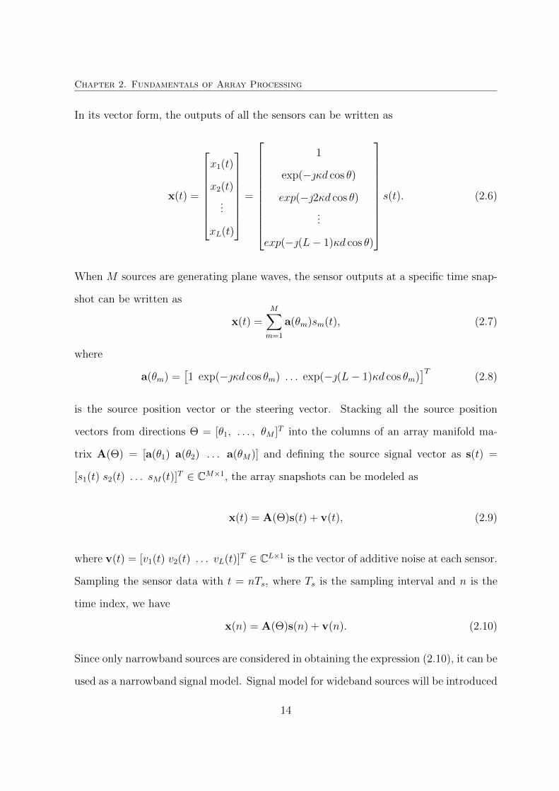
In its vector form, the outputs of all the sensors can be written as
x(t) =
x1(t)
x2(t)
...
xL(t)
=
1
exp(−κd cos θ)
exp(−2κd cos θ)
...
exp(−(L− 1)κd cos θ)
s(t). (2.6)
When M sources are generating plane waves, the sensor outputs at a specific time snap-
shot can be written as
x(t) =M∑m=1
a(θm)sm(t), (2.7)
where
a(θm) =[1 exp(−κd cos θm) . . . exp(−(L− 1)κd cos θm)
]T(2.8)
is the source position vector or the steering vector. Stacking all the source position
vectors from directions Θ = [θ1, . . . , θM ]T into the columns of an array manifold ma-
trix A(Θ) = [a(θ1) a(θ2) . . . a(θM)] and defining the source signal vector as s(t) =
[s1(t) s2(t) . . . sM(t)]T ∈ CM×1, the array snapshots can be modeled as
x(t) = A(Θ)s(t) + v(t), (2.9)
where v(t) = [v1(t) v2(t) . . . vL(t)]T ∈ CL×1 is the vector of additive noise at each sensor.
Sampling the sensor data with t = nTs, where Ts is the sampling interval and n is the
time index, we have
x(n) = A(Θ)s(n) + v(n). (2.10)
Since only narrowband sources are considered in obtaining the expression (2.10), it can be
used as a narrowband signal model. Signal model for wideband sources will be introduced
14

Chapter 2. Fundamentals of Array Processing
in Section 2.3.
In the analysis of observed sensor snapshots, the sensor noise is generally modeled
as a Gaussian random process while the source signals can either be deterministic or
random, depending on application. For random uncorrelated sources, if we define Rss as
the M ×M source covariance matrix, the second-order statistics of the sensor snapshots
is obtained by the array covariance matrix as
R = E{(x(n)− x)(x(n)− x)H} = A(Θ)RssAH(Θ) + Rvv, (2.11)
where x = E{x(n)} is the mean vector of x(n) and Rvv ∈ CL×L is the noise covariance
matrix. For applications with non-Gaussian sources, higher-order statistics of the sen-
sor snapshots preserve additional information which has been exploited for both DOA
estimation [12] and beamforming [13].
2.2 Narrowband Array Processing
In this section, we discuss existing beamforming, DOA estimation and model order esti-
mation techniques for narrowband sources. For such a scenario, the signal model is given
by (2.10). It is important to note that the signal model in (2.10), as well as the techniques
being presented henceforth, are not restricted to uniform linear array geometry.
2.2.1 Beamforming
Beamforming is the process of combining signals from the array elements such that the
source from a specific direction of interest constructively add up while the signals arriving
from other directions are suppressed. The most primitive beamformer is the delay-and-
sum beamformer which compensates for the path delay of a source signal from the desired
15

Chapter 2. Fundamentals of Array Processing
direction before accumulating the compensated outputs. An equivalent phase compensa-
tion can restore the desired signal when processed in the frequency domain. If we denote
the phase compensation as a vector of complex weights, the amplitude of these weights
provide additional degree-of-freedom (DOF) enabling the suppression of interferers from
other directions. A typical narrowband beamformer is shown in Figure 2.2. The objec-
tive of beamforming algorithms is to design the complex weight vector w considering the
design constraints.
Figure 2.2: A typical narrowband beamformer with complex weights.
Design of the beamformer can either be data dependent or independent. Data in-
dependent design leads to the domain area of array pattern synthesis. For real-time
processing, data-dependent adaptive beamformers are advantageous as they incorporate
environmental factors into the design. Here, we briefly discuss minimum variance distor-
tionless response (MVDR) beamformer [14].
As the name suggests, the output of an MVDR beamformer is expected to provide
an undistorted signal from the desired direction while maintaining a minimum output
power. If a(θ0) denotes the steering vector from direction θ0, the source signal from this
direction can be maintained undistorted at the beamformer output with weight vector w
16
Chapter 2. Fundamentals of Array Processing
chosen such that wHa(θ0) = c, where c > 0 is a constant equal to the gain of the array.
Given the beamformer output y(n) = wHx(n), the output power can be expressed as
P = E{y2(n)} = E{|wHx(n)|2}
= wHRw,
(2.12)
where R = E{x(n)xH(n)} is the array covariance matrix of the zero-mean sensor snap-
shots across the array. The weight vector for an MVDR beamformer can therefore be
obtained by solving the following optimization problem:
minimizew
wHRw
subject to wHa(θ0) = c.
(2.13)
The Lagrangian function for this problem is given by
L(w, λ) = wHRw + λ(wHa(θ0)− c
), (2.14)
where λ is the Lagrangian parameter. With R assumed to be a positive definite matrix,
(2.14) is a convex function. Solving for the global minimum of (2.14), we obtained the
solution for w as
w =R−1a(θ0)
aH(θ0)R−1a(θ0). (2.15)
Substituting (2.15) into (2.12), the beamformer output power is given by
Pmvdr =1
aH(θ0)R−1a(θ0). (2.16)
We note that the optimization problem in (2.13) consists of a single linear constraint.
It is straightforward to extend this beamformer to incorporate multiple constraints to, for
17
Chapter 2. Fundamentals of Array Processing
instance, suppress an interference from a known direction. The beamformer is then called
linear constrained minimum variance (LCMV) beamformer. From (2.8), we observe that
the steering vector is a function of source direction, array geometry, signal frequency and
the propagation speed. Extensive work has been done to incorporate robustness to errors
in these factors into the beamformer formulation [15].
2.2.2 DOA Estimation
In the previous section, beamforming is achieved by providing weights corresponding to
the desired source direction in the spatial domain. By evaluating the beamformer output
power for all possible directions, we obtain the spatial spectrum which exhibits distinct
peaks along the source directions. If we denote φ as the scanning direction which sweeps
the entire azimuth range, the spatial spectrum is given by
Pmvdr(φ) =1
aH(φ)R−1a(φ). (2.17)
The expression in (2.17) evaluates the power in each direction φ in contrast to the beam-
forming context where the output power, defined in (2.16), is evaluated only along the
source direction.
The MVDR algorithm and other high resolution spectral estimation techniques such
as linear prediction [16] and maximum entropy [17] have been outperformed by techniques
which exploit eigen structure within the array correlation matrix R. Among them, the
well-known multiple signal classification (MUSIC) algorithm [18] and estimation of signal
parameters via rotational invariance technique (ESPRIT) [19] are discussed here, while
the readers are referred to [2] for a description of other techniques.
18

Chapter 2. Fundamentals of Array Processing
2.2.2.1 MUSIC Algorithm
Since the array covariance matrix R is Hermitian symmetric, it can be subjected to eigen
decomposition as
R = UΛUH , (2.18)
where U and Λ are the eigenvector and eigenvalue matrices, respectively. The eigenvec-
tors in U corresponding to the largest M eigenvalues form the columns of Us, while the
remaining eigenvectors form the noise subspace matrix Un. We therefore have
R =
[Us Un
]Λs 0
0 Λn
UH
s
UHn
= UsΛsU
Hs + UnΛnU
Hn ,
(2.19)
where Λs ∈ CM×M and Λn ∈ CL−M×L−M are the diagonal matrix of signal and noise
subspace eigenvalues. The MUSIC algorithm can be explained based on the following
proposition.
Proposition 2.1 If the sources are not coherent and the uncorrelated additive noise v(n)
has equal variance σ2v across all sensors, then the array manifold matrix A(Θ) and Us
span the same subspace [18].
Under the specified conditions, the array covariance matrix R in (2.11) simplifies to
R = A(Θ)RssAH(Θ) + σ2
vIL. (2.20)
It is easy to show that the range space of the signal subspace eigenvector matrix Us and
that of the array manifold matrix A(Θ) are identical [3]. It therefore follows that the
steering vectors along the source directions θ ∈ Θ are orthogonal to the noise subspace,
19

Chapter 2. Fundamentals of Array Processing
i.e., UHn a(θ) = 0. The spectral MUSIC estimator searches for the M source directions
which are exquisitely orthogonal to the noise eigenvectors over the direction span in the
spatial spectrum given by
Pmusic(φ) =1
|UHn a(φ)|2 . (2.21)
The search over all possible directions can be circumvented by exploiting specific struc-
tures in the array geometry. For a ULA, the spectrum of MUSIC algorithm can be
expressed as a polynomial, the roots of which yields the source directions. Details of this
technique is presented in [2].
2.2.2.2 ESPRIT Algorithm
Estimation of signal parameters via rotational invariance technique (ESPRIT) [19] is a
subspace technique which requires two subarrays for DOA estimation. Elements of the
two subarrays are required to form matched pairs, i.e., the displacement vectors of the
first subarray elements w.r.t. its reference sensor have to be equal to the displacement
vectors of the second subarray elements w.r.t. the corresponding reference sensor. This
condition requires the subarrays to be identical. For simplicity we consider a ULA of
L+ 1 sensors divided into two subarrays. The first L sensors form the first subarray and
the L sensors starting from the second sensor form the second subarray.
Proposition 2.2 Given two matched subarrays whose reference sensors, measured in
wavelengths, are displaced by ∆0, the source directions can be estimated from the eigen-
values of a nonsingular matrix Ψ defining the linear transformation between the first
subarray signal subspace Usx and the second subarray signal subspace Usy.
20

Chapter 2. Fundamentals of Array Processing
The proof for the above proposition provided in [3] shows that the matrix Ψ relates
the signal subspaces of the two subarrays as
UsxΨ = Usy, (2.22)
preserves the source directions in the argument of its eigenvalues. The matrix Ψ can be
estimated in several ways, of which, the total least squares approach requires one to first
define a 2M × L matrix U = [UsxUsy]H . The eigen decomposition of UUH yields the
eigenvalue and eigenvector matrices ΛU and VU, respectively. The eigenvector matrix
can be partitioned into a 2× 2 block matrix as
VU =
V11 V12
V21 V22.
(2.23)
From this partitioned matrix, the estimate of Ψ is obtained as Ψ = −V11V−122 .
Once Ψ is estimated, its eigenvalues provide the M ×M diagonal matrix Φ. From
(??), the source directions are retrieved as
θm = cos−1
(arg(Φm,m)
2π∆0
), m = 1, 2, ...,M, (2.24)
‘where Φm,m denotes the mth diagonal entry of Φ.
The above subspace-based techniques such as MUSIC, ESPRIT and maximum like-
lihood method can be generalized under a unified approach called weighted subspace
fitting (WSF) as shown in [20].
21

Chapter 2. Fundamentals of Array Processing
2.2.3 Model-Order Estimation
The order of the narrowband signal model in (2.10) is equal to the number of sources
present in the scenario. The problem of estimating the number of sources can also be
posed as a detection problem in which it is required to detect all the active sources in
the environment. As studied earlier, several DOA estimation techniques presume the
model order to be known. While several techniques have been proposed for this task, we
briefly review two popular techniques, viz., Akaike information criterion (AIC) [21] and
Rissanen’s minimum description length (MDL) [22] in this section.
One approach to estimate the model order is to perform sequential hypothesis tests
looking for L − q, q = 1, ..., L smallest eigenvalues of R which are equal. A sufficient
statistic for this task is [23],
Lq(q) = N(L− q) ln
{g1(q)
g2(q)
}, (2.25)
where g1(q) = 1L−q
∑Li=q+1 λi and g2(q) =
{∏Li=q+1 λi
} 1L−q
, with λi denoting the ith
eigenvalue of R. For N � L and A(Θ) and Rss of rank q, L − q number of smallest
eigenvalues will be equal resulting in Lq(q) = 0.
The AIC and MDL employ the criteria of (2.25) along with a penalty function related
to the available degrees of freedom. The AIC and MDL functions are given, respectively,
by
LAIC(q) =N(L− q) ln
{g1(q)
g2(q)
}+ q(2L− q), (2.26a)
LMDL(q) =N(L− q) ln
{g1(q)
g2(q)
}+
1
2q(2L− q) logN. (2.26b)
22

Chapter 2. Fundamentals of Array Processing
From these criteria, the model order is estimated as
qAIC =argminq
LAIC(q), (2.27a)
qMDL =argminq
LMDL(q). (2.27b)
The performance of these techniques are susceptible to the number of sensors and sources,
signal strength, spatial separation of sources, signal correlation and the number of snap-
shots. A detailed comparative study of the two techniques has been presented in [2]. In
the presence of coherent sources, the rank deficient Rss adversely affects AIC and MDL.
A modification to MDL has been proposed in [24] for such a scenario.
2.3 Wideband Array Processing
We now consider a wideband signal propagating in a lossless homogeneous medium. The
wave equation at a spatial location r due to the planar wavefront is
s(t, r) = s(t−α.r), (2.28)
where α = 1νu is the slowness vector directed towards the source direction. Depending on
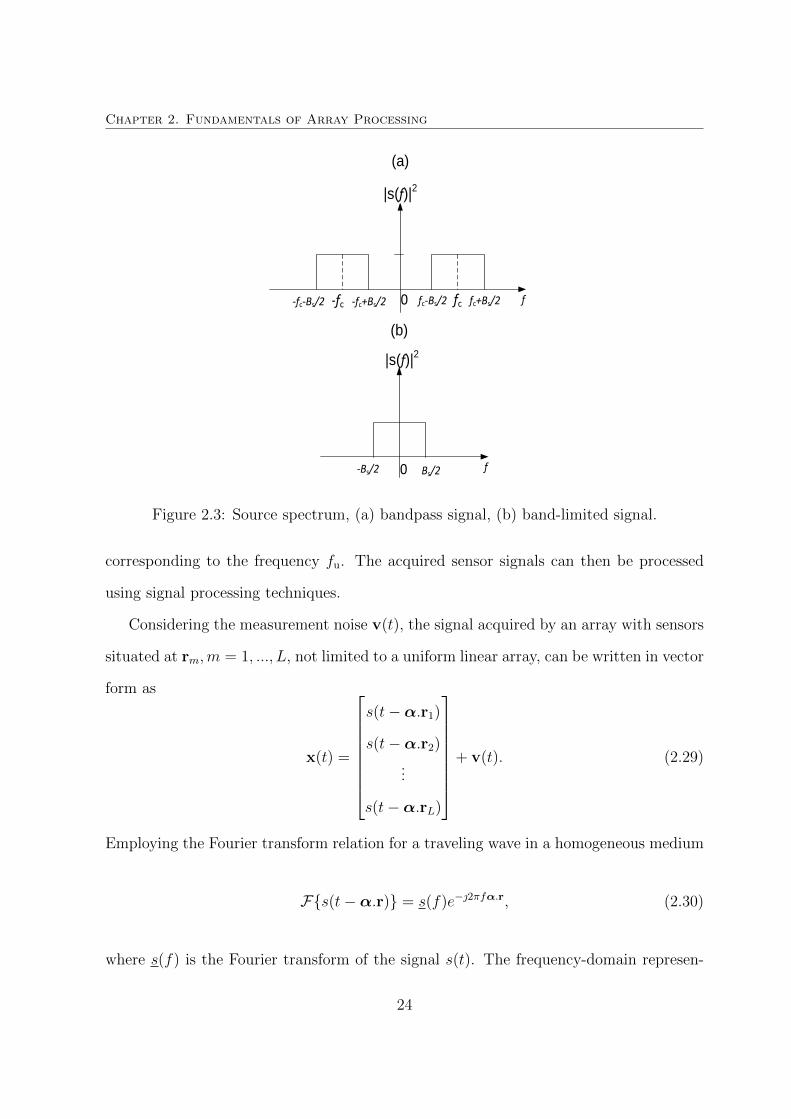
the application, wideband sources can either have band-limited or bandpass spectrum as
shown in Figure 2.3. For a wideband source with bandwidth Bs and having its spectrum
within [fl, fu], the bandpass sampling theorem furnishes an alias-free sampling frequency
of 2fub≥ fs ≤ 2fl
b−1, where b ≤
⌊fuBs
⌋. However, for a bandlimited wideband signal, the
sensor outputs have to be sampled at fs ≥ Bs in order to avoid the presence of aliasing
components. Likewise, it is essential for the sensor array to satisfy Nyquist criterion in
the spatial domain for band-limited wideband sources, d ≤ λu2
, where λu is the wavelength
23
Chapter 2. Fundamentals of Array Processing
0
0 f
|s(f)|2
|s(f)|2
-fc -fc+Bs/2-fc-Bs/2
(a)
(b)
Bs/2 f
fc-Bs/2 fc+Bs/2
-Bs/2
fc
Figure 2.3: Source spectrum, (a) bandpass signal, (b) band-limited signal.
corresponding to the frequency fu. The acquired sensor signals can then be processed
using signal processing techniques.
Considering the measurement noise v(t), the signal acquired by an array with sensors
situated at rm,m = 1, ..., L, not limited to a uniform linear array, can be written in vector
form as
x(t) =
s(t−α.r1)
s(t−α.r2)
...
s(t−α.rL)
+ v(t). (2.29)
Employing the Fourier transform relation for a traveling wave in a homogeneous medium
F{s(t−α.r)} = s(f)e−2πfα.r, (2.30)
where s(f) is the Fourier transform of the signal s(t). The frequency-domain represen-
24
Chapter 2. Fundamentals of Array Processing
tation of (2.29) is then given by the L× 1 vector
x(f) =
e−2πfα.r1
e−2πfα.r2
...
e−2πfα.rL
s(f) + v(f)
= a(f, θ)s(f) + v(f),
(2.31)
where a(f, θ) is the L × 1 steering vector, x(f) and v(f) denote the frequency-domain
representation of the sensor and noise vectors at frequency f . Extending the signal model
in (2.31) for a scenario with M sources from directions Θ = [θ1, ..., θM ], we have
x(f) = A(f,Θ)s(f) + v(f), (2.32)
with A(f,Θ) = [a(f, θ1), . . . , a(f, θM)] and s(f) denoting the array manifold matrix and
the M × 1 source vector, respectively. The spectral density matrix of x(f), Pxx(f) =
E{x(f)xH(f)} is given by
Pxx(f) = A(f,Θ)Pss(f)AH(f,Θ) + Pvv(f), (2.33)
where Pss(f) = E{s(f)sH(f)} and Pvv(f) = E{v(f)vH(f)} are the source and noise
spectral density matrices.
In order to process the wideband data, sensor outputs are critically sampled at fs =
2fu assuming band-limited sources. If the sensor data over a temporal window of size
∆T is subjected to discrete Fourier transform (DFT), a vector of sensor outputs x(k, l)
known as the frequency-domain snapshot at each discrete frequency bin index k within
the signal bandwidth and time-frame index l is obtained. The signal model is then given
25

Chapter 2. Fundamentals of Array Processing
by
x(k, l) = A(fk,Θ)s(k, l) + v(k, l). (2.34)
The covariance matrix at bin index k can be estimated using J frequency-domain snap-
shots from the corresponding frequency as
R(fk) =1
J
J∑l=1
x(k, l)xH(k, l). (2.35)
2.3.1 Beamforming
At each frequency, we note that the wideband signal model degenerates to a narrowband
model in (2.10). Therefore, a straightforward approach to achieve wideband beamforming
is to perform narrowband beamforming at each frequency bin. The beamformer output
in time domain can then be estimated by inverse DFT of the narrowband beamformer
outputs.
Alternatively, a time-domain wideband beamformer introduces a filter at each sensor
output prior to the constructive summation of the outputs as shown in Figure 2.4(a).
This technique was first proposed by Frost [25]. Figure 2.4(b) shows a D-tap FIR filter
wi,m,m = 0, ..., D − 1 at the output of ith sensor. The design of these filters to obtain a
desired frequency and wave number response is the problem in hand. The response for
the broadband beamformer is given by
b(θ, f) =L∑l=1
Wl(f)e−2πfτl(θ), (2.36)
where τl(θ) is the propagation delay w.r.t. the origin of the sensor array, Wl(f) is the
frequency response of the filter for the lth sensor. With the desired source direction
known apriori, it is a common practice to pre-steer the sensor outputs such that the
26

Chapter 2. Fundamentals of Array Processing
source is synthetically shifted to the broadside of the array. This allows one to focus on
designing a broadside beamformer with required interference suppression from all other
directions.
2.3.1.1 Frost Beamforming
Let xl(n) be the output of the lth sensor, appropriately presteered to have the desired
signal in the broadside of the array. At a tap delay m, we can define a spatial vector
x(n−m) = [x1(n−m) x2(n−m) . . . xL(n−m)]T . Vectorizing the snapshots at all the
D-delays, we obtain a spatio-temporal snapshot with D previous time samples from nth
sample as
x(n) = [xT (n) xT (n− 1) . . . xT (n−D + 1)]T . (2.37)
Since the array outputs are presteered, the look-direction spatial vector at a given
tap-delay is a vector of ones 1L. This results in a cumulated filter weight h(m) =∑Li=1wi,m,m = 0, ..., D − 1. The frequency response of the wideband array can be con-
trolled by designing the filter response of h(m). If g(m),m = 0, ..., D − 1 denote the
filter coefficients of the desired frequency response, we can construct a constraint for the
weights of the mth tap delay across the sensors such that
wH cm = g(m), (2.38)
where w = [wT0 ... w
TD−1]T is the weight vector across the entire time-delay structure with
wm = [w1,m w2,m ... wL,m]T denoting the vector of weights across the array at tap m and
cm = [0TL, ...,1TL, ...0
TL]T is the LD×1 constraint vector with the mth block of L elements
corresponding to a vector of ones and zeros elsewhere. Likewise, an LD ×D constraint
matrix C can be defined as
C = [c0 c1 . . . cD−1], (2.39)
27
Chapter 2. Fundamentals of Array Processing
using which, we have D constraints given by
CT w = g, (2.40)
where g = [g(0) . . . g(D − 1)]T is the filter response of the desired frequency response.
The optimal set of filter weights w can be obtained by solving the following optimiza-
tion problem:
minimizew
wHRxxw
subject to CT w = g.
(2.41)
The obtained solution assures a linear distortionless response over the signal bandwidth.
As shown in [2, p. 657], this formulation can directly be extended to tackle interferences
by introducing additional constraints over the D − 1 tap delays.
For a wideband beamformer, an error in the nominal source direction can result in
signal cancellation at the beamformer output. In order to introduce robustness to source
position error, the unity response in the look direction can be broadened using additional
constraints. While several techniques have been proposed to achieve this [3], introducing
linear derivative constraints which enforce the derivative of the power pattern w.r.t. the
bearing angle to zero [26] was one of the foremost techniques.
A generalized sidelobe canceller (GSC) beamformer can be extended to broadband
source scenario as well. The first path ensures a fixed beam with specific frequency
response while the auxiliary path blocks the desired signal by placing a null in the cor-
responding direction. The L− 1 beams at the output of the blocking pre-filter are then
passed through a tapped delay line filter. The filters in the auxiliary path are adaptively
designed to minimize the overall beamformer output power. In the discussed beamform-
ers, the frequency response of the filters are designed such that the distortionless response
from the look direction is emphasized. On the contrary, frequency invariant beamform-
28
Chapter 2. Fundamentals of Array Processing
ers (FIB) are designed to have a constant frequency response over the signal bandwidth
along with spatial filtering [27]. The underlying idea is to transform the sensor signals
into phase mode, wherein the dependence on frequency is removed by appropriately-
designed filters. The beamforming coefficients which follows the filtered signals can be
estimated by employing the trapezoidal rule. The design of FIR filters following each sen-
sor output are shown to be dilation factors of a reference filter [28]. Under the frequency
invariance conditions, it is important to note that the FIR filters cannot be designed for
any arbitrary array. However, it is possible to exploit inherent structures in some array
geometries to design filters with frequency invariant characteristics. The design of filters
with uniform concentric circular arrays for beamforming and DOA estimation has been
shown in [29].
2.3.2 DOA Estimation
As described earlier, broadband array processing process spatio-temporal snapshots x(n)
instead of spatial snapshots used for narrowband DOA estimation. However, broadband
DOA estimation using spatio-temporal snapshots has the following limitations [30]:
(i) The signal subspace dimension of the covariance matrix R = E{x(n)xH(n)} will be
a composite subspace greater than the number of sources present in the scenario.
(ii) With increase in the tap-delays, the dimensionality of the problem increases the
computational complexity.
Due to the first limitation, the segregation of signal subspace and noise subspace is not
clearly defined. Therefore, the problem is generally addressed in the frequency domain.
Transforming the sensor outputs into frequency domain converts the filtering process at
each sensor into multiplication of a complex weight at each frequency. Moreover, the
frequency-domain snapshots follow a narrowband signal model at each frequency bin.
29
Chapter 2. Fundamentals of Array Processing
We now review some of the existing techniques which serve as baseline algorithms in
future chapters.
2.3.2.1 Incoherent Signal Subspace Method (ISSM)
The foremost technique for wideband DOA estimation is to estimate source directions in
small narrowband portions of the signal bandwidth using any of the narrowband subspace
techniques and unify them incoherently to obtain a final estimate [31]. This is achieved
by an arithmetic or geometric mean of the spatial spectra across the signal bandwidth
as follows:
PISSM−AM(φ) =1
1B
∑fufk=fl
1L−M
∑Li=M+1 |aH(fk, φ)ei(fk)|2
,
PISSM−GM(φ) =1
1B
∏fufk=fl
(1
L−M∑L
i=M+1 |aH(fk, φ)ei(fk)|2)1/B
,(2.42)
where ei(fk), i = M+1, ..., L are the noise eigenvectors for bin index k and B denotes the
number of narrowband frequency components across the signal bandwidth [fl, fu]. The
subscripts “ISSM-AM” and “ISSM-GM” denote the arithmetic and geometric mean ver-
sions of the spatial spectrum. As highlighted in [31], PISSM−AM(φ) exhibits a peak when
a(fk, φ) is “almost orthogonal” to all the noise eigenvectors across all the frequency bins.
On the contrary, the geometric mean estimator is observed to exhibit a peak if the noise
eigenvectors are almost orthogonal to a(fk, φ) in at least one of the narrowband compo-
nents over the signal bandwidth. Therefore PISSM−GM(φ) will have a higher resolution
but lower accuracy than the arithmetic mean estimator. The power variations in differ-
ent narrowband segments adversely affects the ISSM spectrum. Moreover, the technique
cannot resolve coherent sources which occur in the presence of multipath.
In [32], a new incoherent DOA estimation technique which does not require one to
30
Chapter 2. Fundamentals of Array Processing
determine the number of sources has been proposed. The arithmetic mean of the nar-
rowband cost function across the signal bandwidth has been used to estimate wideband
source directions. This technique assumes source nonstationarity in order to develop a
cost function which is independent of the model order. While the solution is well suited
for speech sources, the assumptions withhold its extension to stationary source scenario,
in which case, the technique degenerates to ISSM [31]. Furthermore, the incoherent
summation across frequencies bins, carries the limitations of ISSM to this technique in
handling the coherent sources.
2.3.2.2 Coherent Signal Subspace (CSS) Approach
In this approach [33–35], the wideband data is first decomposed into non-overlapping
narrowband components. The data from each frequency bin index k is then transformed
to a reference frequency f0 using pre-designed focussing matrices T(fk,Θinit) given by
y(k) = T(fk,Θinit)x(k)
= T(fk,Θinit)A(fk,Θ)s(k) + T(fk,Θinit)v(k),
(2.43)
where Θinit is the vector of approximate initial source directions. The transformed data
covariance matrices, given by Ry(fk) = E{y(k)yH(k)}, are averaged over the entire
frequency band of interest [fl, fu] to obtain
Rcssm =
fu∑fk=fl
Ry(fk)
=
fu∑fk=kl
T(fk,Θinit)R(fk)TH(fk,Θinit).
(2.44)
31

Chapter 2. Fundamentals of Array Processing
The focussing matrices are designed such that
T(fk,Θinit)A(fk,Θ) = A(f0,Θ). (2.45)
This allows (2.44) to be written as
Rcssm = A(f0,Θ)
{fu∑
fk=fl
Rss(fk)
}AH(f0,Θ) + Rv, (2.46)
where Rss(fk) is the source covariance matrix obtained at frequency fk and Rv is the
transformed noise covariance matrix. We note that the first term in (2.46) is similar to
the covariance matrix obtained for a narrowband signal model at f0. Assuming additive
noise across the sensors to be uncorrelated and have equal power σ2v(fk), the second term
is given by
Rv =
fu∑fk=fl
σ2v(fk)T(fk,Θinit)T
H(fk,Θinit). (2.47)
In order to estimate the source locations, Rv is first estimated using (2.47). The eigen-
vectors ei, i = 1, ..., L and eigenvalues λi, i = 1, ..., L of the matrix pencil (Rcssm,Rv)
are obtained by solving the generalized eigenvalue problem. With the number of sources
assumed to be known, the narrowband MUSIC spectrum is used to estimate the source
directions with noise subspace eigenvectors Un = [eM+1 . . . eL] and the steering vectors
evaluated at f0.
From (2.45) we note that the design of focussing matrices requires approximate source
directions. The design of focussing matrix has therefore gained significant interest [36–
38]. While the details of focussing matrix design are not discussed here, one suggested
approach [36] is to provide initial estimates from the peaks of the MVDR spatial spectrum
along with the spatial points distant from the peaks by 0.125 times the beamwidth.
It is well known that CSSM performs well at low SNRs. Furthermore, the coherent
32

Chapter 2. Fundamentals of Array Processing
summation of focussed covariance matrices restores the rank of Rcssm, thus enabling the
technique to resolve coherent sources. However, a large error in the provided initial
estimates reflects in the bias of the DOA estimates.
2.3.2.3 Frequency Invariant Beamforming-based DOA Estimation
This technique, proposed in [39], adopts a beamspace approach for wideband DOA es-
timation. The basic idea relies in forming G (M < G < L) beams from the sensor
outputs using frequency invariant beamformers (FIB). The used FIB ensures frequency
invariance, as a consequence of which, coherent summation of data across frequency is
achieved. DOA parameters can then be estimated using any narrowband estimator.
With the array geometry and source bandwidth known, G FIBs are designed to span
the entire spatial range. Defining a matrix C(fk) = [b1(fk), ...,bG(fk)] with G beam-
shaping filter responses bj(fk), j = 1, ..., J at frequency fk, the beam-shaped output
z(k) ∈ CG×1 is given by
z(k, l) = CH(fk)x(k, l)
= CH(fk)s(k, l) + CH(fk)v(k, l).
(2.48)
The corresponding covariance matrix is
Rzz(fk) = Ac(fk,Θ)Rss(fk)AHc (fk,Θ) + Rv(fk), (2.49)
where Ac(fk,Θ) = CH(fk)A(fk,Θ) and Rv(fk) = CH(fk)E{v(k)vH(k)}C(fk) is the cor-
related noise after transformation. Since C(fk) is designed such that the array manifold
33
Chapter 2. Fundamentals of Array Processing
representation becomes frequency invariant, i.e., Ac(fk,Θ) = Ac(Θ),∀fk ∈ [fl, fu],
Rfib =
fu∑fk=fl
Rzz(fk)
= Ac(Θ)
{ fu∑fk=fl
Rss(fk)
}AH
c (Θ) +
fu∑fk=fl
Rv(fk).
(2.50)
From (2.50) and (2.46), it is evident that FIB-based DOA estimation employs a similar
approach to tackle coherent sources in the scenario by restoring the rank of source co-
variance matrix. Assuming the noise covariance matrix to be known, narrowband DOA
estimation can be performed similar to that performed for CSSM post-focussing.
2.3.2.4 Steered Covariance Matrix-MVDR (STCM-MVDR) [40]
In this technique, DOA estimation is accomplished via a beamformer derived from
the coherent processing of data across the signal bandwidth which is shown to pro-
vide improved stability and accuracy [40]. Towards this, the array covariance matrix
R(fk) = E{x(k, l)xH(k, l)}, evaluated at each frequency within the signal bandwidth
[fl, fu] are first steered to the look direction φ and then accumulated to form the steered
covariance matrix (STCM) given by
R(φ) =
fu∑fk=fl
TH(fk, φ)R(fk)T(fk, φ), (2.51)
where T(fk, φ) = diag(a(fk, φ)) is the diagonal steering matrix. This coherent summation
over several frequency bins enhances the signal power over the background noise prior to
the estimation. The spatial response is then given by [40]
P (φ) =1
1TLR−1(φ)1L. (2.52)
34

Chapter 2. Fundamentals of Array Processing
Although STCM-MVDR is expected to exhibit good resolution, the subspace-based tech-
niques provide superior resolution. Furthermore, performing matrix inverse in each look
direction is computationally expensive. However, it is important to note that the spatial
spectrum of this technique is insensitive to the errors in estimated model order.
2.3.2.5 Test for Orthogonality of Projection Subspaces (TOPS)
TOPS [41] is a relatively new wideband DOA estimation technique that has been classified
as a noncoherent signal subspace method. While this technique cannot resolve coherent
sources, the approach is quite different from other techniques.
At a reference frequency f0, the covariance matrix estimated from frequency domain
snapshots is decomposed into signal and noise subspaces Us(k0) and Un(k0) assuming the
number of sources to be known. The signal subspace is transformed to each of the other
frequencies within the signal bandwidth [fl, fu] using a transformation matrix T(fk, φ)
which compensates for the frequency in each direction
Us(fk, φ) = T(fk, φ)Us(f0), k = 1, ..., B, (2.53)
where δfk = fk − f0 and B is the number of frequency bins under consideration. A
direction dependent matrix Dφ is then defined as
Dφ =[U′Hs (f1, φ)Un(f1) U′Hs (f2, φ)Un(f2) . . . U′Hs (fB, φ)Un(fB)
], (2.54)
where U′s(fk, φ) =[IL−(aH(fk, φ)a(fk, φ))−1a(fk, φ)aH(fk, φ)
]Us(fk, φ). The matrix Dφ
has the following property for the source and non-source directions:
(i) if φ ∈ Θ, Dφ becomes rank deficient,
(ii) if φ /∈ Θ, Dφ is a full rank matrix.
35

Chapter 2. Fundamentals of Array Processing
Source directions can therefore be estimated using
θtops = arg minφ
1
σmin(φ), (2.55)
where σmin(φ) is the smallest singular value of Dφ.
While this technique has found to outperform CSSM for mid and high SNR ranges,
the technique cannot resolve sources at low SNR conditions. Furthermore, this technique
is highly sensitive to any errors in model-order estimation. Since this is a noncoherent
approach, the technique cannot handle coherent sources.
2.3.2.6 Beamforming-Framework Wideband MUSIC algorithm (BFW-MUSIC) [42]
This is another technique which estimates wideband source directions from time-domain
snapshots. Unlike FIB-based technique, this technique uses narrowband beamforming
framework for DOA estimation, i.e., spatial snapshots x(n) are used instead of spatio-
temporal snapshots x(n). For time-domain processing, as mentioned earlier, the steering
vector for a given direction will span a subspace obtained over the signal bandwidth
{a(f, φ),∀f ∈ [fl, fu]}. This technique introduces robustness to the steering variations
with frequency, thus enabling frequency invariance.
The narrowband MUSIC algorithm is first reformulated as a beamformer [42]
minimizewφ
‖wφ − a(φ)‖22
subject to UHs wφ = 0,
(2.56)
where wφ is the weight vector solution. The above beamformer, which introduces deep
nulls along the source directions, is steered in each look direction and wφ is evaluated.
36

Chapter 2. Fundamentals of Array Processing
Source directions can be estimated from the peaks in the direction finding function
DF(φ) = 10log10
1
|wHφ a(φ)| . (2.57)
The formulation is directly extended to wideband case by introducing the following con-
straints,
wHφ
∂a(f, φ)
∂f
∣∣∣f=f0
= 0
...
wHφ
∂Pa(f, φ)
∂fP
∣∣∣f=f0
= 0,
(2.58)
where ∂P a(f,φ)∂fP
is the P th derivative of the steering vector in the direction φ. These
derivative constraints widen the nulls along the frequency axis, making the weight vec-
tor insensitive to wideband components. This technique is advantageous in estimating
directions of sources with varying signal bandwidth with limited number of time-domain
snapshots. However, the challenge appears in providing the extended signal subspace Us
of R for DOA estimation.
The above discussed techniques are observed to exploit the orthogonality between
the signal and noise subspaces for DOA estimation, either directly or indirectly. Alterna-
tively, direction parameters can also be estimated in the maximum likelihood sense [43].
However, the complete search over the parameter space in this approach is computation-
ally very expensive. A modified maximum likelihood approach with limited search is
therefore proposed in [44], which can simultaneously estimate the model order and the
source directions. Although the technique reduces the search space, the estimates are
searched starting from a maximally hypothesized number of sources. Therefore, the com-
putational complexity is proportional to the maximally hypothesized number of sources
and the array size. In [45], a unified approach for beamforming, DOA estimation and
37

Chapter 2. Fundamentals of Array Processing
model order estimation has been proposed in which a posteriori distribution parame-
terized with source parameters, directions and the number of sources is obtained from
the likelihood function. Markov chain Monte-Carlo approach is used to estimate these
parameters simultaneously. The computational complexity and the iterative nature does
not make this technique attractive.
In summary, the large computational cost of maximum likelihood techniques can be
substituted with subspace-based wideband DOA estimation techniques such as CSSM.
However, accurate model order has to be estimated for these techniques to provide reliable
estimates at low SNR conditions.
2.3.3 Model-Order Estimation
Determining the number of sources is a primitive problem, solving which propels the
task of DOA estimation. As studied in Section 2.2.3, the most common criteria used for
model-order estimation in the narrowband scenario is by observing the multiplicity of the
smallest eigenvalue of the array covariance matrix. If q denotes the smallest eigenvalue
multiplicity, M = L − q is the estimated number of sources. Evidently, it is more
challenging to estimate the number of sources in a wideband scenario by combining the
information over the entire signal bandwidth. This problem has been treated with either
standalone algorithms [31, 33] or as one of the outcomes from joint model order-DOA
estimation schemes [43–45].
The foremost approach [31] adopts a composite likelihood ratio which is a function of
M obtained by the ratio of arithmetic and geometric means of the eigenvalues obtained
for array covariance matrices over the entire signal bandwidth. Due to the incoherent
processing, the performance of this technique is not acceptable at low SNR values. More-
over, the presence of coherent sources cannot be identified by this technique. These two
limitations are circumvented in [33] by using AIC on eigenvalues obtained by solving
38

Chapter 2. Fundamentals of Array Processing
the generalized eigenvalue decomposition (Rcssm,Rv). Besides restoring the rank in the
presence of coherent sources, this technique exhibits better detection at low SNRs due
to the coherent summation across all the frequency bins. The problem of simultaneous
estimation of model order and source directions has been formulated in [43] as a multiple-
hypothesis test with test statistics derived from the generalized likelihood ratio principle.
Although the performance is acceptable at low SNRs, the computational complexity lim-
its its applicability. As discussed before, the modification to limit its search [44] reduces
the complexity marginally.
39
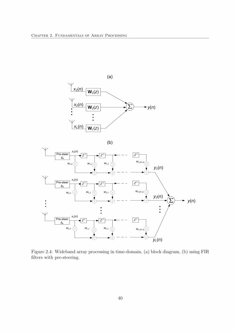
Chapter 2. Fundamentals of Array Processing
w1,(D-1)
wL,(D-1)
yL(n)
w1,1
xL(n)
x2(n)
x1(n)
y(n)
W1(z)
W2(z)
WL(z)
(a)
(b)
x1(n)Pre-steer
∆1Z-1
w1,0
Z-1 Z-1
x2(n)Pre-steer
∆2Z-1 Z-1 Z-1
w2,(D-1)
xL(n)Pre-steer
∆LZ-1 Z-1 Z-1
y(n)
y1(n)
y2(n)
w1,2
w2,0 w2,1 w2,2
wL,0 wL,1 wL,2
Figure 2.4: Wideband array processing in time-domain, (a) block diagram, (b) using FIRfilters with pre-steering.
40

Chapter 3
Narrowband DOA Estimation
without Order Selection
3.1 Introduction
In the previous chapter, it was observed that the subspace-based techniques for nar-
rowband DOA estimation seek knowledge of the number of sources present for accurate
estimation of source directions. As a result, the estimated source directions are sus-
ceptible to model-order estimation errors. More recently, a DOA estimator based on a
beamforming-framework has been proposed in [9] which is insensitive to the estimated
model order. It was remarked that the working principle of this technique follows that
of the MUSIC algorithm and hence was referred to as “MUSIC-like” algorithm. How-
ever, detailed analysis of this technique which asserts the MUSIC-like operation is not
provided.
In this chapter, we first review the technique proposed in [9] and perform a detailed
analysis of its optimization problem. We first show that the steered response power of this
technique differs from the MVDR algorithm and then demonstrate that the underlying
41

Chapter 3. Narrowband DOA Estimation without Order Selection
working principle of the technique is similar to that of the MUSIC algorithm. The bounds
for the sole parameter is derived from the solution under the desired spatial spectrum
conditions. From the insights obtained, we observe that the weight vector estimated in
each direction resides in the noise subspace. Exploiting this fact, we construct a matrix
W of weight vectors obtained from arbitrary directions, the columns of which, spans only
the noise subspace. This matrix can substitute the use of noise subspace in subspace-
based techniques, thus circumventing the order-selection problem. Furthermore, the
estimation of weight vector from limited number of directions significantly reduces the
computational complexity of the proposed technique (MUSIC-W algorithm) over the
MUSIC-like algorithm which solves a generalized eigenvalue problem in each azimuth
direction. The performance of MUSIC-like and MUSIC-W algorithms are evaluated in
comparison with the MUSIC algorithm.
Within the scope of the thesis, this chapter plays a significant role. With a detailed
understanding of the MUSIC-like algorithm, we realize the potential of this algorithm to
be extended for wideband DOA estimation. This extension is very appealing considering
the fact that model-order estimation in wideband scenario is much more challenging and
computationally expensive.
3.2 MUSIC-like Narrowband DOA Estimator
3.2.1 Formulation
The algorithm proposed in [9] solves the following optimization problem in each look
direction,
minimizewφ
wHφ Rwφ
subject to wHφ
{a(φ)aH(φ) + βIL
}wφ = c,
(3.1)
42

Chapter 3. Narrowband DOA Estimation without Order Selection
where c, β > 0 are constants. Although this optimization problem reduces to the MVDR
algorithm when β = 0, the working principle significantly differs from MVDR for all
β > 0. While the objective function minimizes the beamformer output power in the
look direction, the quadratic equality constraint regulates the look-direction power gain
‖wHφ a(φ)‖2
2 in relation with the objective function. An in-depth discussion on this relation
will be provided in the next section. The Lagrangian function can be constructed as
L(wφ, χ) = wHφ Rwφ − χ(wH
φ {a(φ)aH(φ) + βIL}wφ − c), (3.2)
where χ is the Langrangian multiplier. Equating the gradient of L(wφ, χ) w.r.t. the
weight vector to zero, the solution is given by the eigenvector corresponding to the
minimum eigenvalue χmin of the generalized eigenvalue (GEV) problem
Rwφ = χmin{a(φ)aH(φ) + βIL}wφ. (3.3)
Since the weight vector is a generalized eigenvector of the matrix pencil[R,{a(φ)aH(φ) + βIL
}],
the solution vector obtained from (3.3) is invariant to the rescaling wφ → αwφ. We there-
fore consider ‖wφ‖2 = 1 henceforth without loss of generality. Furthermore, we note that
the solution wφ in (3.3) is independent of the value of c, which is implicitly assigned
to c = ‖wHφ a(φ)‖2
2 + β‖w‖22. As will be shown in the next section, the solution vec-
tor wφ,∀φ, resides in the noise subspace with appropriate choice of β. This again is
in contrast to weight vector solution for MVDR along the source directions due to the
distortionless response constraint. The algorithm in (3.1) therefore employs the direction
finding function given by
P (φ) = 10log10
1
|wHφ a(φ)|2 , (3.4)
43
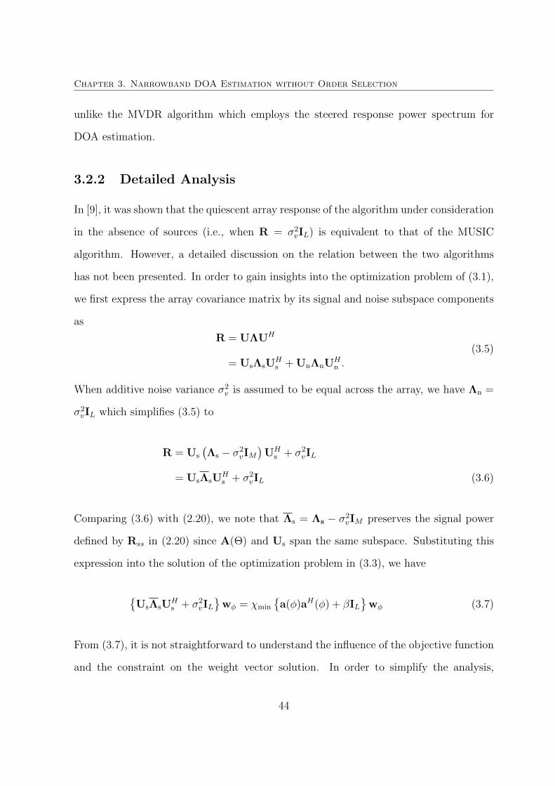
Chapter 3. Narrowband DOA Estimation without Order Selection
unlike the MVDR algorithm which employs the steered response power spectrum for
DOA estimation.
3.2.2 Detailed Analysis
In [9], it was shown that the quiescent array response of the algorithm under consideration
in the absence of sources (i.e., when R = σ2vIL) is equivalent to that of the MUSIC
algorithm. However, a detailed discussion on the relation between the two algorithms
has not been presented. In order to gain insights into the optimization problem of (3.1),
we first express the array covariance matrix by its signal and noise subspace components
as
R = UΛUH
= UsΛsUHs + UnΛnU
Hn .
(3.5)
When additive noise variance σ2v is assumed to be equal across the array, we have Λn =
σ2vIL which simplifies (3.5) to
R = Us
(Λs − σ2
vIM)
UHs + σ2
vIL
= UsΛsUHs + σ2
vIL (3.6)
Comparing (3.6) with (2.20), we note that Λs = Λs − σ2vIM preserves the signal power
defined by Rss in (2.20) since A(Θ) and Us span the same subspace. Substituting this
expression into the solution of the optimization problem in (3.3), we have
{UsΛsU
Hs + σ2
vIL}
wφ = χmin
{a(φ)aH(φ) + βIL
}wφ (3.7)
From (3.7), it is not straightforward to understand the influence of the objective function
and the constraint on the weight vector solution. In order to simplify the analysis,
44
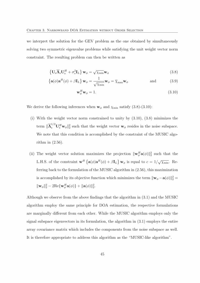
Chapter 3. Narrowband DOA Estimation without Order Selection
we interpret the solution for the GEV problem as the one obtained by simultaneously
solving two symmetric eigenvalue problems while satisfying the unit weight vector norm
constraint. The resulting problem can then be written as
{UsΛsU
Hs + σ2
vIL}
wφ =√χminwφ (3.8){
a(φ)aH(φ) + βIL}
wφ =1√χmin
wφ = χmaxwφ and (3.9)
wHφ wφ = 1. (3.10)
We derive the following inferences when wφ and χmin satisfy (3.8)-(3.10):
(i) With the weight vector norm constrained to unity by (3.10), (3.8) minimizes the
term ‖Λ1/2
s UHs wφ‖2
2 such that the weight vector wφ resides in the noise subspace.
We note that this condition is accomplished by the constraint of the MUSIC algo-
rithm in (2.56).
(ii) The weight vector solution maximizes the projection ‖wHφ a(φ)‖2
2 such that the
L.H.S. of the constraint wH{a(φ)aH(φ) + βIL
}wφ is equal to c = 1/
√χmin. Re-
ferring back to the formulation of the MUSIC algorithm in (2.56), this maximization
is accomplished by its objective function which minimizes the term ‖wφ−a(φ)‖22 =
‖wφ‖22 − 2Re{wH
φ a(φ)}+ ‖a(φ)‖22.
Although we observe from the above findings that the algorithm in (3.1) and the MUSIC
algorithm employ the same principle for DOA estimation, the respective formulations
are marginally different from each other. While the MUSIC algorithm employs only the
signal subspace eigenvectors in its formulation, the algorithm in (3.1) employs the entire
array covariance matrix which includes the components from the noise subspace as well.
It is therefore appropriate to address this algorithm as the “MUSIC-like algorithm”.
45
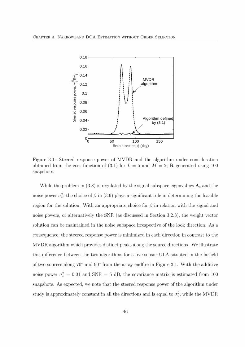
Chapter 3. Narrowband DOA Estimation without Order Selection
0 50 100 1500
0.02
0.04
0.06
0.08
0.1
0.12
0.14
0.16
0.18
Scan direction, (deg)
Stee
red
resp
onse
pow
er, w
H R
w
MVDR algorithm
Algorithm defined by (3.1)
Figure 3.1: Steered response power of MVDR and the algorithm under considerationobtained from the cost function of (3.1) for L = 5 and M = 2; R generated using 100snapshots.
While the problem in (3.8) is regulated by the signal subspace eigenvalues Λs and the
noise power σ2v , the choice of β in (3.9) plays a significant role in determining the feasible
region for the solution. With an appropriate choice for β in relation with the signal and
noise powers, or alternatively the SNR (as discussed in Section 3.2.3), the weight vector
solution can be maintained in the noise subspace irrespective of the look direction. As a
consequence, the steered response power is minimized in each direction in contrast to the
MVDR algorithm which provides distinct peaks along the source directions. We illustrate
this difference between the two algorithms for a five-sensor ULA situated in the farfield
of two sources along 70◦ and 90◦ from the array endfire in Figure 3.1. With the additive
noise power σ2v = 0.01 and SNR = 5 dB, the covariance matrix is estimated from 100
snapshots. As expected, we note that the steered response power of the algorithm under
study is approximately constant in all the directions and is equal to σ2v , while the MVDR
46
Chapter 3. Narrowband DOA Estimation without Order Selection
response provides peaks along the source directions. This explains the use of (3.4) for
DOA estimation instead of the steered power response.
In order to further analyze the constraint of (3.1), we express it in terms of the
complementary subspaces of R. Assuming ‖a(φ)‖22 = 1 without loss of generality, the
steering vector projection matrix is given by
Paφ = a(φ)(aH(φ)a(φ))−1aH(φ) = a(φ)aH(φ). (3.11)
Noting that Paφ = PaφPaφ , we can introduce the complementary subspaces of the co-
variance matrix using the relation IL = UsUHs + UnU
Hn in the look direction gain as
wHφ a(φ)aH(φ)wφ = wH
φ PaφILPaφwφ
= wHφ Paφ
{UsU
Hs + UnU
Hn
}Paφwφ
= ‖UHs Paφwφ‖2
2 + ‖UHn Paφwφ‖2
2. (3.12)
The constraint and the direction finding functions which incorporate this term can be
written as
‖UHs wφ‖2
2 + ‖UHn wφ‖2
2 + β‖wφ‖22 = c (3.13)
DF(φ) = 10 log10
1
‖UHs wφ‖2
2 + ‖UHn wφ‖2
2
, (3.14)
where wφ = Paφwφ. From the illustration in Figure 3.1, it is observed that the optimiza-
tion problem successfully minimizes wHφ Rwφ for all the directions φ, thus enforcing the
weight vector to reside in the noise subspace. It therefore follows that ‖UHs Paφwφ‖2
2 → 0
in each direction φ. Along the source directions in particular, we have the steering
vector residing completely in the signal subspace while the noise subspace contains the
47

Chapter 3. Narrowband DOA Estimation without Order Selection
0 50 100 150
0
50
100
150
200
250
300
350
400
Scan direction, (deg)
Spatia
l Spect
rum
(dB
)
MUSIC-like algorithmMUSIC algorithm
Figure 3.2: Spatial spectrum of MUSIC and MUSIC-like algorithms for L = 5 sensorswith synthetic covariance matrix generated using (2.20).
weight vector solution, i.e., R{wφ} ∩ R{a(φ)} = ϕ, where ϕ denotes the null set. As a
consequence, we have wφ = 0, which induces distinct peaks in DF(θ) along the source
directions similar to the MUSIC algorithm.
We illustrate this similarity between the two algorithms for the simulation setup
employed for Figure 3.1 with L = 5 sensors and M = 2 sources. The covariance matrix
is however generated directly from the source and noise powers using (2.20) instead of
using the array snapshots. The spatial spectrum for MUSIC and MUSIC-like algorithms
plotted in Figure 3.2 are observed to be almost identical. As the covariance matrix
deviates from (2.20) due to finite number of snapshots, the spatial spectrum of MUSIC-
like algorithm deviates from the MUSIC algorithm. This difference in the performance
of the two algorithms is due to the difference in respective formulations although their
asymptotic performances are similar. This phenomenon is observed for the same setup
48

Chapter 3. Narrowband DOA Estimation without Order Selection
0 50 100 150-10
-5
0
5
10
15
20
Scan direction, (deg)
P(
) (d
B)
Music-like algorithm
Music algorithm
Figure 3.3: Spatial spectrum of MUSIC and MUSIC-like algorithms with 100 snapshotsfor L = 5,M = 2 and SNR=5 dB.
with L = 5, M = 2 along 70◦ and 90◦, but with 100 sensor snapshots. The sensor
outputs are corrupted with additive Gaussian noise maintained at an SNR of 5 dB.
Deferring the discussion on the choice of β for now, the spatial spectra obtained for
MUSIC and MUSIC-like algorithms are plotted in Figure 3.3. We note that the spectrum
floor for both the algorithms are still maintained at the same level. Although the source
direction peaks are prominent in the spectrum for both the techniques, the magnitude is
significantly reduced when compared to Figure 3.2. The difference in the spectrum of the
two techniques becomes more prominent at lower SNR conditions where the use of one
of the complementary subspaces in MUSIC is advantageous over MUSIC-like algorithm
which uses the entire covariance matrix as will be shown Section 3.4.
49

Chapter 3. Narrowband DOA Estimation without Order Selection
3.2.3 Bounds for β
The bounds for β were derived in [9] considering the possibility of the steering vector
residing in different subspaces under three different cases. We alternatively derive the
bounds from the solution to the GEV in (3.3)
(a(φ)aH(φ) + βIL)wφ = χ−1minRwφ. (3.15)
With R being positive definite, (3.15) takes the form
R−1(a(φ)aH(φ) + βIL)wφ = χ−1minwφ,
{C + βB}wφ = χ−1minwφ,
(3.16)
where B = R−1 and C = Ba(φ)aH(φ). Hence, the above results in
wHφ {C + βB}wφ
‖wφ‖22
= χ−1min (3.17)
denoting the maximum eigenvalue of {C + βB}. For P (φ) to provide peaks along
source directions, wφ has to satisfy |wHφ a(φ)| = 0. Consequently, we require Cwφ =
Ba(φ)aH(φ)wφ = 0, ∀φ ∈ Θ which is satisfied when
wHφ {C + βB}wφ
‖wφ‖22
≈ βwHφ Bwφ
‖wφ‖22
. (3.18)
This condition is assured when
βwHφ Bwφ
‖wφ‖22
�wHφ Cwφ
‖wφ‖22
. (3.19)
50
Chapter 3. Narrowband DOA Estimation without Order Selection
Since R is a full rank matrix, we note that
rank(C) = rank(R−1Paφ) = min{rank(R−1), rank(Paφ)}. (3.20)
With rank(Paφ) = 1, the rank of C is equal to 1. Under this condition, we have χC,max =
tr{C}, where we explicitly denote the maximum eigenvalue of C as χC,max. The highest
lower bound for the inequality in (3.19) will therefore be
βwHφ Bwφ
‖wφ‖22
� χC,max = tr{C}. (3.21)
Furthermore, when (3.18) is satisfied, we havewHφ Bwφ
‖wφ‖22= χB,max. The highest lower bound
for β considering all the source directions is therefore given by
β > maxφ∈Θ
tr{Ba(φ)aH(φ)}χB,max
= maxφ∈Θ
aH(φ)R−1a(φ)
χR−1,max
, (3.22)
where we have used the identity tr{EFG} = tr{FGE} for any three matrices E,F,G.
It is interesting to note that the term (aH(φ)R−1a(φ))−1 signifies the signal power along
the source direction. Rewriting the R.H.S. of (3.22) in terms of the minimum eigenvalue
of R which defines the noise power, we have
β > maxφ∈Θ
χR,min
(aH(φ)R−1a(φ))−1= max
φ∈Θ
σ2v
(aH(φ)R−1a(φ))−1,
β >1
SNR.
(3.23)
We therefore infer that the parameter β is guided by the reciprocal of SNR.
For directions φ /∈ Θ, it is equally important to ensure Cwφ 6= 0, failing which false
peaks will appear in the spatial spectrum. In view of this, β cannot be arbitrarily high
51

Chapter 3. Narrowband DOA Estimation without Order Selection
and has to be constrained such that
βwHφ Bwφ
‖wφ‖22
<wHφ Cwφ
‖wφ‖22
, or
βχB,max < χC,max.
(3.24)
Since (3.24) has to be maintained for all φ /∈ Θ, the lowest upper bound for β is obtained
as
β < minφ/∈Θ
aHφ R−1aφ
χB,max
. (3.25)
Therefore, the bound for β is given by
maxφ∈Θ
aH(φ)R−1a(φ)
χR−1,max
< β < minφ/∈Θ
aH(φ)R−1a(φ)
χR−1,max
βmin < β < βmax.
(3.26)
Emphasizing on the peaks along the source directions, a good choice for β can be obtained
w.r.t. the minimum value of aH(φ)R−1a(φ) as
β = ηminφ
aH(φ)R−1a(φ)
χR−1,max
, (3.27)
where η > 1 ensures reliable DOA estimates when β is contained within the upper bound.
3.3 Proposed DOA Estimation Technique (MUSIC-
W)
In the previous section, we studied that the working principle of the MUSIC-like algo-
rithm is similar to that of MUSIC algorithm asymptotically. Even with finite number
of snapshots, it was noted that the spatial spectrum of the MUSIC-like algorithm at
52

Chapter 3. Narrowband DOA Estimation without Order Selection
moderate SNR conditions approached that of the MUSIC algorithm when β is chosen
within the derived bounds. Under adverse conditions however, the covariance matrix
deviates significantly from the ideal conditions assumed in the earlier analysis which may
adversely affect the estimation accuracy. Although this algorithm is insensitive to the
errors in model-order estimation, it is computationally intensive to evaluate the general-
ized eigenvector in each look direction, compared to the evaluation of a single SVD in the
case of MUSIC algorithm. In this section, we propose a new technique developed over
the MUSIC-like algorithm which provides improved performance over the latter and has
reduced the computational complexity.
Interpreting the GEV problem solved by the MUSIC-like algorithm in each look di-
rection as two eigenvalue problems ((3.8) and (3.9)) being simultaneously solved, it is
noted that the generalized eigenvector and the corresponding eigenvalue have to satisfy
both the problems. Since we have a(φ) ∈ R{Us} ∪ R{Un} along the non-source di-
rections, the solution weight vector yields |wHφ a(φ)|2 6= 0. Along the source directions
however, we have the steering vector completely residing in the signal subspace. While
the objective function ensures the weight vector solution to reside in the noise subspace,
it is contradicting to maximize the look-direction power gain ‖wHφ a(φ)‖2
2. Due to this
contrast between the two symmetric eigenvalue problems along the source directions,
the generalized eigenvalue χmin corresponding to the solution vector is expected to be
large compared to the value of χmin in all other directions. In order to verify this phe-
nomenon, we study the generalized eigenvalue corresponding to the solution vector for
the previous simulation setup with L = 5 sensors and two sources along 70◦ and 90◦.
With 100 snapshots and SNR= 5 dB, χmin is plotted against the scan direction φ in
Figure 3.4. We note an increase in χmin along the source direction over a nominal value
in all directions. This increase in eigenvalue indicates the difficulty for the weight vector
solution along the source direction to achieve concurrent minimization of |Λ1/2
s UHs wφ|2
53

Chapter 3. Narrowband DOA Estimation without Order Selection
0 50 100 1500.05
0.1
0.15
0.2
0.25
0.3
0.35
0.4
0.45
Scan direction, (deg)
min
Figure 3.4: Generalized eigenvalue χmin corresponding to the solution weight vector plot-ted against the scan direction for L = 5,M = 2 with 100 snapshots and SNR=5 dB.
and the maximization of |wHφ a(θ)|2. It therefore follows that the choice of β is crucial in
providing a solution which results in |wHφ a(φ)|2 = 0 required for showing distinct peaks
in DF(φ) along the source directions. Under adverse conditions, the estimation accuracy
is susceptible to the choice of β and the number of snapshots used.
It was earlier observed that the weight vector solution resides in the noise subspace
for both source and non-source directions. While each vector wφ is orthogonal to the
signal subspace, the vector may be contained in a subset of noise eigenvectors of R unlike
the minimum norm solution. We therefore construct a weight vector matrix given by
W = [wφ1 wφ2 . . . wφK ], (3.28)
where the solutions from K different directions are used to construct the matrix. Al-
54

Chapter 3. Narrowband DOA Estimation without Order Selection
though the columns of this weight vector matrix are not orthogonal, with K > L −M ,
the range space of W is expected to be the same as the noise subspace of R. We can
therefore replace the use of noise subspace in existing subspace-based DOA estimation
techniques such as MUSIC and minimum norm algorithms. In order to emulate the
MUSIC algorithm, the source directions can then be estimated as the peaks of
Pmusic−w(φ) = 10 log10
1
aH(φ)WWHa(φ), (3.29)
where the subscript “music-w” is used to denote the proposed algorithm which uses
weight matrix W to approximate MUSIC algorithm. The performance of this technique
will rely on the number of weight vectors K used to construct W. This is because,
sufficient number of weight vectors are required to ensure that the weight vector matrix
W and the signal subspace eigenvector matrix Un have the same range space, failing
which will give rise to false peaks in the spatial spectrum. We therefore require at least
K ≥ L−M vectors to construct W. Since the weight vector evaluated in each direction
over the entire azimuth range reside in the noise subspace, constructing W with K ≥ L
will still provide similar performance, thus avoiding the need for the model order.
For the earlier setup with L = 8 and M = 2, we now study the spatial spectrum
of the proposed MUSIC-W algorithm in comparison with the MUSIC and MUSIC-like
algorithms. We employ K = 8 weight vectors from equidistant directions over an azimuth
span of 10◦ to 170◦ to construct W. At an SNR of 5 dB, the spatial spectra for the three
techniques obtained for N = 100 snapshots is plotted in Figure 3.5. We observe that
the proposed technique provides prominent peaks along the source directions similar to
the MUSIC and MUSIC-like algorithms. However, the spectrum floor for the proposed
technique differs from the other techniques which have similar spatial spectra over the
entire azimuth range. The spectrum floor obtained for the MUSIC-W is susceptible to
55

Chapter 3. Narrowband DOA Estimation without Order Selection
0 50 100 150-5
0
5
10
15
20
25
30
35
Scan direction , (deg)
P(
), d
B
MUSIC-W
MUSIC
MUSIC-like
Figure 3.5: Spatial spectrum of MUSIC-W algorithm in comparison with that of MUSICand MUSIC-like algorithms at SNR=5 dB.
the directions from which the weight vectors are used to construct the matrix W.
The above phenomenon is illustrated with the previous simulation setup for two cases
with the weight vectors chosen from an azimuth range of 10◦ to 90◦ for the first case and
90◦ to 170◦ for the second. The spatial spectra are plotted in Figure 3.6(a) and (b),
respectively. For the first case, we note that the spectrum floor is suppressed only in
the corresponding region. While the absence of significant false peaks in the spectrum
ensures that the range space R{W} is equal to the noise subspace, the use of weight
vectors from a specific region in the azimuth range emphasizes the suppression of noise
floor corresponding to the same azimuth range. Since W cannot control the spectrum
floor in the complementary region, we observe an increase in the corresponding segment
in both the subplots of Figure 3.6.
56
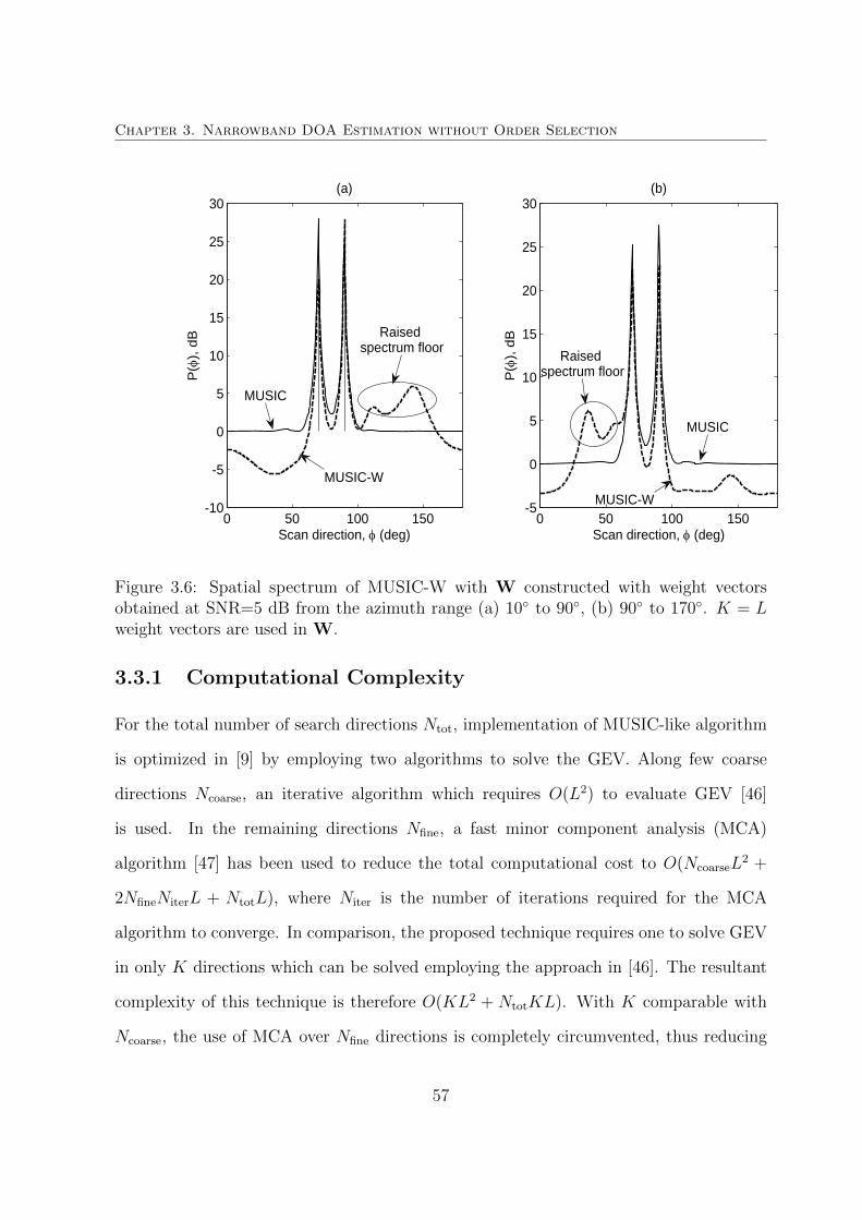
Chapter 3. Narrowband DOA Estimation without Order Selection
0 50 100 150-10
-5
0
5
10
15
20
25
30
Scan direction, (deg)
P(
), d
B(a)
0 50 100 150-5
0
5
10
15
20
25
30
Scan direction, (deg)
P(
), d
B
(b)
Raised spectrum floor
Raised spectrum floor
MUSIC-W
MUSIC-W
MUSIC
MUSIC
Figure 3.6: Spatial spectrum of MUSIC-W with W constructed with weight vectorsobtained at SNR=5 dB from the azimuth range (a) 10◦ to 90◦, (b) 90◦ to 170◦. K = Lweight vectors are used in W.
3.3.1 Computational Complexity
For the total number of search directions Ntot, implementation of MUSIC-like algorithm
is optimized in [9] by employing two algorithms to solve the GEV. Along few coarse
directions Ncoarse, an iterative algorithm which requires O(L2) to evaluate GEV [46]
is used. In the remaining directions Nfine, a fast minor component analysis (MCA)
algorithm [47] has been used to reduce the total computational cost to O(NcoarseL2 +
2NfineNiterL + NtotL), where Niter is the number of iterations required for the MCA
algorithm to converge. In comparison, the proposed technique requires one to solve GEV
in only K directions which can be solved employing the approach in [46]. The resultant
complexity of this technique is therefore O(KL2 + NtotKL). With K comparable with
Ncoarse, the use of MCA over Nfine directions is completely circumvented, thus reducing
57
Chapter 3. Narrowband DOA Estimation without Order Selection
the computations significantly. With the evaluation of GEV reduced to only K directions,
the computational cost involved in the proposed algorithm is comparable with the MUSIC
algorithm which requires O(ML2 + L(L−M)Ntot + (L−M)Ntot).
3.4 Simulation Results
In this section, we evaluate the performance of the analyzed MUSIC-like algorithm and
the proposed MUSIC-W algorithm in comparison with the MUSIC algorithm. It was
observed in Section 3.2.3 that β is implicitly related to the SNR. We therefore expect the
performance of MUSIC-like algorithm to be influenced by the choice of β, and hence η.
We now study the performance of the MUSIC-like estimator over various values of η from
the root-mean-squared error (RMSE) of the estimates, evaluated over 100 trials. Across
all the simulations, we consider the scenario which consists of an eight-sensor ULA and
three sources at 50◦, 65◦ and 110◦ unless specified. We fix the number of snapshots to 100
and study the effect of η, defined after (3.27), at SNR=−5, 0 and 5 dB. Figure 3.7 shows
the RMSE of estimates averaged across the three sources and plotted against η for the
MUSIC-like algorithm. At a moderate SNR of 5 dB, we note that any choice of η which
ensures β within the bounds has marginal effect on the estimation accuracy. However,
for SNRs of 0 dB and −5 dB, a large RMSE is observed when η < 1.5 suggesting that the
parameter introduces significant error in the accuracy when chosen close to the derived
lower bound. The estimation error gradually increases for η > 1.5 as β approaches the
upper bound.
For the proposed MUSIC-W algorithm, the weight vectors used for W are evaluated
with η = 1.5 based on this study. Besides this factor, the performance of the MUSIC-W
algorithm is also influenced by the number of weight vectors used to construct W and the
azimuth region over which these vectors are evaluated. While the influence of azimuth
58

Chapter 3. Narrowband DOA Estimation without Order Selection
1.2 1.4 1.6 1.8 2 2.2 2.4 2.6 2.80
0.5
1
1.5
2
2.5
RM
SE
(deg)
SNR =-5dBSNR = 0dBSNR = 5dB
Figure 3.7: RMSE of source estimates using the MUSIC-like algorithm plotted against ηat various SNR values.
region on the spatial spectrum of MUSIC-W algorithm was observed in Figures 3.5 and
3.6, we now study the influence of the number of weight vectors in W on the performance
of the technique. For the earlier simulation setup used to generate Figure 3.7 with L = 8,
the estimation accuracy of the MUSIC-W technique is evaluated as a function of K. The
RMSE of the three source estimates are averaged and plotted against K at SNR values
of −5 dB, 0 dB and 5 dB in Figure 3.8. When the SNR is 5 dB, we note that the choice
of K > L is not of high importance. However, for SNRs of 0 and −5 dB, the estimation
error is observed to decrease for K > L. This indicates that limiting the number of weight
vectors marginally deteriorates the estimation performance at low SNR conditions since
the weight vectors may not be completely orthogonal to the signal subspace. Therefore,
employing W with K ≥ L is suggested for MUSIC-W algorithm to provide accurate
estimates.
59

Chapter 3. Narrowband DOA Estimation without Order Selection
6 8 10 12 14 16 18 200
0.2
0.4
0.6
0.8
1
1.2
1.4
1.6
1.8
2
K
RM
SE
(deg)
SNR = 5dB
SNR = 0dB
SNR = -5dB
Figure 3.8: RMSE of source estimates obtained with the MUSIC-W algorithm plottedagainst K at various SNR values.
Since the weight vector solutions for both MUSIC-like and MUSIC-W algorithms
are obtained by solving the GEV problem, the spatial spectrum cannot be expressed
as a closed-form expression in terms of the covariance matrix and steering vector un-
like the MVDR or MUSIC algorithms. We therefore study the performance of these
algorithms with simulations observing the estimation accuracy and the probability of re-
solving closely-situated sources. We first study the estimation accuracy by observing the
root mean squared error (RMSE) plotted against the SNR before analyzing the prob-
ability of resolution. We conducted a Monte Carlo simulation with 100 trials. For a
simulation setup with an eight-sensor ULA and three sources at 50◦, 70◦ and 80◦, the
DOA estimates for MUSIC-like algorithm are obtained with η = 1.5. We have used
K = 10 vectors to construct W for the proposed MUSIC-W algorithm. The RMSE of
source estimates are obtained with 100 snapshots for various SNR values and is compared
60

Chapter 3. Narrowband DOA Estimation without Order Selection
with the MVDR and MUSIC algorithms in Figure 3.9.
-5 0 5 10 15 20 25 300
0.5
1
1.5
SNR (dB)
RM
SE
(de
g)(a) Source 1
-5 0 5 10 15 20 25 300
0.5
1
1.5
2
2.5
SNR (dB)
RM
SE
(de
g)
(b) Source 2
-5 0 5 10 15 20 25 300
0.5
1
1.5
2
SNR (dB)
RM
SE
(de
g)
(c) Source 3
MUSICMUSIC-WMUSIC-likeMVDR
MUSICMUSIC-WMUSIC-likeMVDR
MUSICMUSIC-WMUSIC-likeMVDR
Figure 3.9: RMSE of source estimates plotted against SNR for the MUSIC-like, MUSIC-W, MVDR and MUSIC algorithms.
With the clear distinction of the signal and noise subspaces known, we note that
the MUSIC algorithm has the best estimation performance and sets the bench mark
for other techniques. Due to the poor resolution capabilities of the MVDR algorithm,
61

Chapter 3. Narrowband DOA Estimation without Order Selection
we note that the RMSE of the obtained DOA estimates for second and third sources is
significantly larger than all the other techniques. We observe that the source direction
estimates obtained by the MUSIC-like algorithm exhibit large RMSE at low SNR con-
ditions. Although the RMSE decreases with an increase in the SNR, the non-diagonal
noise covariance matrix with limited number of snapshots withhold its performance from
approaching that of the MUSIC algorithm. It is interesting to note that the MUSIC-W
algorithm shows better estimation accuracy over MUSIC-like algorithm when the SNR is
increased. This advantage in the performance is due to the prime difference between the
two algorithms. Along the source directions, it was earlier studied that the generalized
eigenvalue of the MUSIC-like optimization problem is significantly large compared to
all other directions, thus indicating the difficulty in simultaneously satisfying both the
eigenvalue problems. This condition will therefore introduce marginal error in the DOA
estimates of the MUSIC-like algorithm. Since the matrix W employed in the MUSIC-
W algorithm is constructed with weight vectors obtained from arbitrary directions, the
range space of this matrix is confined to the noise subspace. The estimation accuracy of
MUSIC-W DOA estimates is therefore observed to approach that of MUSIC as the SNR
is increased. At lower SNR conditions, the solution vectors in W may not completely
reside in the noise subspace thus introducing marginal errors in the estimates.
We now study the capability of these techniques to resolve two closely-situated sources.
The simulation setup involves L = 8 sensor ULA and two sources situated at 70◦ and
76◦ from the array axis. The two sources are considered to be resolved when
|θ1 − θ1| ≤θ2 − θ1
2and
|θ2 − θ2| ≤θ2 − θ1
2,
(3.30)
where θ1 and θ2 are the DOA estimates corresponding to the source directions θ1 and
62

Chapter 3. Narrowband DOA Estimation without Order Selection
θ2 respectively, obtained from the estimator. The probability of resolution is evaluated
as the ratio of the number of times the algorithm resolves over the total number of
Monte Carlo trials. With 100 sensor snapshots synthesized, the probability of resolution,
evaluated over 150 trials, is plotted against SNR in Figure 3.10.
-30 -20 -10 0 10 20 300
0.1
0.2
0.3
0.4
0.5
0.6
0.7
0.8
0.9
1
SNR (dB)
Pro
babi
lity
of R
esol
utio
n
MUSIC-like algorithm
MUSIC with AIC
MUSIC-W algorithm
MVDR algorithm
Figure 3.10: The probability of resolving two closely situated sources with 100 snapshots.
We note that the MUSIC-like algorithm and the proposed MUSIC-W algorithm can
resolve the two source directions under adverse conditions where the MUSIC algorithm
supported with AIC for model order estimation fails to resolve the sources. Furthermore,
it is observed that MVDR requires 8 − 10 dB higher SNR to resolve the two sources.
This simulation asserts the advantage of the proposed technique and the MUSIC-like
algorithm over the MUSIC algorithm in conjunction with existing model order estimation
techniques under adverse conditions.
63

Chapter 3. Narrowband DOA Estimation without Order Selection
We next study the effect of the number of snapshots used on the estimation accuracy
of these algorithms for the scenario with L = 8 sensor ULA and three sources situated
at 50◦, 70◦ and 80◦. Setting the SNR at 5 dB, the RMSE for each source direction
is plotted in Figure 3.11 over increasing number of snapshots. We note that the DOA
estimation accuracy of the MUSIC-like and MUSIC-W algorithms improves with an
increase in the number of snapshots. However, we observe that the performance of the
MUSIC-like algorithm does not approach that of the MUSIC algorithm. This is due to
the non-diagonal noise covariance matrix obtained even when the number of snapshots is
significantly large. In contrast, the performance of the MUSIC-W algorithm approaches
that of the MUSIC algorithm when the number of snapshots is large. Due to the limited
capability of the MVDR algorithm to resolve the closely-situated sources, we note that
the MVDR estimates exhibit large RMSE error when the SNR is 5 dB.
When the SNR is increased to 15 dB, we note that the performance of the MVDR and
the MUSIC-W algorithms approach that of the MUSIC algorithm while the performance
of the MUSIC-like algorithm exhibits larger RMSE even when the number of snapshots
is significantly large. This difference is again due to the small deviation of the noise
covariance matrix from being a diagonal matrix. We also note that the RMSE of MUSIC-
W decreases with increase in the number of snapshots and outperforms the MVDR
algorithm even at 15 dB SNR.
3.5 Conclusion
In this chapter, we have presented a mathematical analysis of the MUSIC-like algorithm
starting from its optimization problem and have shown that the working principle of this
technique is similar to that of the MUSIC algorithm when the effect of finite snapshots
is not considered for the estimation of the array covariance matrix. The bounds for the
64

Chapter 3. Narrowband DOA Estimation without Order Selection
parameter β have been rederived to ensure reliable estimates. From the insights obtained,
we then proposed a new technique developed over the working principle of the MUSIC-
like algorithm. The performance of the proposed MUSIC-W algorithm is observed in
simulations to outperform the MUSIC-like algorithm with lesser computational cost.
With the insights obtained from this chapter, we identify the possibility of extending
the MUSIC-like formulation for wideband DOA estimation. Considering the advantage of
circumventing the model order estimation, we dedicate the next two chapters to develop
wideband DOA estimation techniques based on this technique. The bounds for β derived
in Section 3.2.3 can directly be extended to wideband source scenarios.
65

Chapter 3. Narrowband DOA Estimation without Order Selection
102
103
10-2
10-1
100
Number of snapshots
RM
SE
(deg)
(a) Source 1
MUSIC
MUSIC-like
MUSIC-W
MVDR
102
103
10-2
10-1
100
Number of snapshots
RM
SE
(deg)
(b) Source 2
MUSIC
MUSIC-like
MUSIC-W
MVDR
102
103
10-2
10-1
100
Number of snapshots
RM
SE
(deg)
(c) Source 3
MUSIC
MUSIC-like
MUSIC-W
MVDR
SNR = 15dB
SNR = 15dB
SNR = 5dB
SNR = 5dB
SNR = 5dB
SNR = 15dB
Figure 3.11: The RMSE of source estimates plotted against snapshots for the MUSIC-like, MUSIC-W, MUSIC and MVDR algorithms.
66

Chapter 4
Time-Domain Wideband DOA
Estimation
4.1 Introduction
The problem of estimating wideband source directions from sensor snapshots is an inte-
gral part of many applications considering the fact that most of the real-world signals
are wideband in nature. As studied in Section 2.3, the problem definition and the signal
model for wideband DOA estimation are an extension of their narrowband counterpart.
Since elegant solutions are available in the literature for narrowband DOA estimation,
wideband DOA estimation is in general accomplished by employing narrowband algo-
rithms either directly [31] or indirectly [33]. The appealing high resolution achieved
by subspace-based narrowband techniques requires precise knowledge of the model or-
der. The inaccuracy and computation complexity of model order estimation in wideband
scenario requires an alternative approach to tackle the problem.
From the wideband data, parameter estimation can either be accomplished by inco-
herent processing of estimates obtained at each frequency [31] or by coherent processing
67

Chapter 4. Time-Domain Wideband DOA Estimation
of data, followed by DOA estimation [33] as studied in Section 2.2.2. The latter approach
generally outperforms the former under adverse SNR conditions due to an increase in
signal power obtained by summing the coherent covariance matrices across the signal
bandwidth. In coherent signal subspace method (CSSM), the focussing matrices trans-
form data from different frequencies to a reference frequency prior to the joint processing.
However, this technique requires initial approximate estimates of source directions for the
design of focussing matrices. Under adverse conditions, large errors in the initial esti-
mates introduce bias to the estimates. The frequency-invariant DOA estimation proposed
in [39] is equivalent to coherent processing of the wideband data. Nevertheless, it is dif-
ficult to design filters with frequency-invariant property for arbitrary array geometries.
The number of wideband sources present in the scenario has been estimated in [33] em-
ploying either the AIC or MDL criterion on the coherently averaged covariance matrix.
However, if the initial estimates deviate from the true source directions, estimation of
the model order and hence the DOA estimates will be adversely affected.
In this chapter, we provide a new approach to coherently process the wideband data
across the signal bandwidth. This is accomplished by approximating the array manifold
at a frequency within the signal bandwidth w.r.t. a reference frequency using Taylor series
expansion. This approximation, detailed in Section 4.2, permits us to have a time-domain
signal model for wideband DOA estimation. The expression for the corresponding data
covariance matrix, consists of a coherent component at the reference frequency along with
additional derivative components. We then propose to extend the optimization problem
of the MUSIC-like algorithm for wideband DOA estimation in Section 4.3. This enables
one to obtain DOA estimates without estimating the model order. We also perform
a detailed analysis of the optimization problem which enables one to understand the
working principle of the proposed technique. Computer simulations and corresponding
discussions are presented in Section 4.5.
68

Chapter 4. Time-Domain Wideband DOA Estimation
4.2 Array Manifold Approximation for Wideband Sig-
nal Model
The wideband signals acquired by the sensor array can be modeled in frequency domain
as shown in (2.32). From the Fourier transform relation, the continuous-time sensor
signals can be expressed using (2.32) as
x(t) =
∫ ∞−∞
x(f)e2πftdf
=
∫ ∞−∞
A(f,Θ)s(f)e2πftdf + v(t),
(4.1)
where v(t) =∫∞−∞ v(f)e2πftdf is the additive noise vector, uncorrelated with the sources.
It is important to note that the vectors a(f, θ) in A(f,Θ) corresponding to each source
direction are continuous functions of frequency. The steering vector at a frequency f in
the proximity of a reference frequency f0 can hence be approximated using Taylor series
expansion up to the P th order as
a(f, θ) ≈ a(f0, θ) +P∑p=1
(δf)p
p!
∂p
∂f pa(f, θ)
∣∣∣f=f0
, (4.2)
where ∂p
∂fpa(f, θ) is the pth-order derivative of the steering vector w.r.t. frequency and
δf = f − f0 is the frequency deviation from f0. Correspondingly, the array manifold
matrix can be written as
A(f,Θ) ≈ A(f0,Θ) +P∑p=1
(δf)p
p!
∂p
∂f pA(f,Θ)
∣∣∣f=f0
, (4.3)
where the matrix ∂p
∂fpA(f,Θ) =
[∂p
∂fpa(f, θ1) . . . ∂p
∂fpa(f, θM)
]is the pth-order derivative
array manifold. If the steering vector at each frequency over the entire signal bandwidth
69

Chapter 4. Time-Domain Wideband DOA Estimation
is approximated with the P th-order Taylor series, we can substitute (4.3) into (4.1) giving
x(t) ≈∫ ∞−∞
{A(f0,Θ) +
P∑p=1
(δf)p
p!
∂p
∂f pA(f,Θ)
∣∣∣f=f0
}s(f)e2πftdf + v(t). (4.4)
The discrete-time sensor snapshots can be obtained by replacing Fourier transform in (4.4)
with an F−point discrete Fourier transform as
x(n) ≈ 1
F
F−1∑k=0
{A(f0,Θ) +
P∑p=1
(δfk)p
p!
∂p
∂f pA(f,Θ)
∣∣∣f=f0
}s(fk)e
2πkn/F + v(n), (4.5)
where fk denotes the frequency corresponding to bin index k. The array covariance
matrix can then be expressed as
R = E{x(n)xH(n)
}≈ E
{[1
F
F−1∑k=0
(A(f0,Θ) +
P∑p=1
(δfk)p
p!
∂p
∂f pA(f,Θ)
∣∣∣f=f0
)s(fk)e
j 2πknF + v(n)
][
1
F
F−1∑k=0
(A(f0,Θ) +
P∑p=1
(δfk)p
p!
∂p
∂f pA(f,Θ)
∣∣∣f=f0
)s(fk)e
j 2πknF + v(n)
]H}.
(4.6)
70

Chapter 4. Time-Domain Wideband DOA Estimation
Assuming that the source spectrum is uncorrelated across frequency bins, i.e., E{s(f1)sH(f2)} =
0,∀f1 6= f2, (4.6) simplifies to
R ≈ 1
F 2
F−1∑k=0
P∑p,q=0
(δfk)p
p!
∂p
∂f pA(f,Θ)
∣∣∣f=f0
Rss(fk)(δfk)
q
q!
∂p
∂f qAH(f,Θ)
∣∣∣f=f0
+ σ2vIL
≈ 1
F 2A(f0,Θ)
{ F−1∑k=0
Rss(fk)
}AH(f0,Θ)
+2
F 2Re
{F−1∑k=0
P∑p=1
(δfk)p
p!A(f0,Θ)Rss(fk)
∂p
∂f pA(f,Θ)
∣∣∣Hf=f0
}
+1
F 2
F−1∑k=0
P∑p,q=1
(δfk)p
p!
∂p
∂f pA(f,Θ)
∣∣∣f=f0
Rss(fk)(δfk)
q
q!
∂p
∂f qA(f,Θ)
∣∣∣Hf=f0
+ σ2vIL,
(4.7)
where Rss(fk) is the source covariance matrix at frequency fk, σ2v is the noise variance
assumed to be equal across the array and Re{.} denotes the real part of the expression
within. We note that the data from the entire signal bandwidth is coherently averaged
in the first term. Besides improving the SNR, this term restores the rank of the averaged
source covariance matrix when the sources are highly correlated as shown in [33]. The
second and third terms contain derivatives arising due to the array manifold approxima-
tion. These additional terms may increase the eigenvalue spread of R, making it difficult
to estimate the model order employing conventional techniques.
For a given array geometry, if the pth derivative of the steering vector a(f, θ) w.r.t.
frequency evaluated at the reference frequency f0 is denoted as
dp(f0, θ) =∂pa(f, θ)
∂f p
∣∣∣∣f=f0
, (4.8)
71

Chapter 4. Time-Domain Wideband DOA Estimation
a matrix with pth-order derivatives from all the source directions can be formed as
Dp(Θ) =∂p
∂f pA(f,Θ)
∣∣∣∣f=f0
=[dp(f0, θ1) dp(f0, θ2) . . . dp(f0, θM)
].
(4.9)
The covariance matrix in (4.7) can then be written as
R ≈ 1
F 2
[A(f0,Θ)
{ F−1∑k=0
Rss(fk)
}AH(f0,Θ) + 2
F−1∑k=0
Re
{ P∑p=1
(δfk)p
p!A(f0,Θ)Rss(fk)D
Hp (Θ)
}
+P∑
p,q=1
Dp(Θ)
{ F−1∑k=0
(δfk)p+q
p!q!Rss(fk)
}DHq (Θ)
]+ σ2
vIL.
(4.10)
Note that this approximation is valid over a small signal bandwidth across which δf is
small. When the signal bandwidth is large, finite order Taylor series approximation may
introduce error resulting in estimation inaccuracy.
4.3 Proposed Technique
It is interesting to note from (4.10) that the expression for the wideband data covariance
matrix deviates from its narrowband counterpart only due to the presence of the second
term, suppression of which, reduces the problem to a coherently averaged narrowband
DOA estimation problem. Referring to the BFW-MUSIC algorithm discussed in Sec-
tion 2.3.2.6, it is interesting to note that the linear derivative constraints are precisely
aimed at annulling the effect of these terms. Although BFW-MUSIC is efficient in sup-
pressing these terms, the optimization problem is susceptible to the choice of the signal
subspace dimension. This is because, it may not be optimal to choose the dimension of
signal subspace for R expressed in (4.10) to be equal to the model order. We therefore
consider the structure of a MUSIC-like formulation for wideband DOA estimation, which
72

Chapter 4. Time-Domain Wideband DOA Estimation
does not explicitly require one to define the signal subspace dimension.
4.3.1 Formulation
We first define a matrix Df0,φ with derivatives of steering vectors up to the P th-order
evaluated at f0 from a given scan direction φ as
Df0,φ =[d1(f0, φ) d2(f0, φ) . . . dP (f0, φ)
]. (4.11)
With projection matrix of Df0,φ constructed as
PDφ= Df0,φ(DH
f0,φDf0,φ)−1DH
f0,φ,
the sensor snapshots x(n) are then projected onto the derivative vector space, yφ(n) =
PDφx(n), which can loosely be termed as derivative-transformed data snapshots. Since
the columns of PDφspan a P−dimensional subspace, the rank of the covariance matrix
Ry(φ) = E{yφ(n)yHφ (n)
}= PDφ
RPHDφ
(4.12)
is restricted to P with its eigenvectors spanning only the derivative vector space.
From the analysis of narrowband MUSIC-like algorithm in Section 3.2.2, it was noted
that minimizing the beamformer output power in the look direction enforces the weight
vector solution to reside in the noise subspace. Besides this orthogonality to signal sub-
space, the weight vector is now required to be robust against frequency variation. There-
fore, we propose a new formulation for wideband DOA estimation by incorporating (4.12)
73

Chapter 4. Time-Domain Wideband DOA Estimation
as
minimizewφ
wHφ Rwφ + ζwH
φ Ry(φ)wφ
subject to wHφ
{a(f0, φ)aH(f0, φ) + βIL
}wφ = c,
(4.13)
where ζ, β, c > 0 are constants which will be discussed subsequently. Based on the
eigenvalue spread of R, the first term in the objective function wHφ Rwφ minimizes the
projection of wφ onto the composite signal subspace. The inclusion of the second term
provides additional emphasis on the derivative vector space, thus ensuring the weight
vector to be invariant to frequency variations. The solution to this problem is obtained
by setting the gradient of the Lagrangian function
L(wφ, χ) = wHφ
(R + ζRy(φ)
)wφ + χ
(wHφ a(f0, φ)aH(f0, φ)wφ + β‖wφ‖2
2 − c), (4.14)
where χ is the Lagrangian parameter, with respect to the conjugate of wφ to zero. The
eigenvector corresponding to the minimum eigenvalue χmin of the generalized eigenvalue
(GEV) problem,
(R + ζRy(φ)
)wφ = χmin
(a(f0, φ)aH(f0, φ) + βIL
)wφ (4.15)
serves as the optimal weight vector in each scan direction. Since the solution weight
vector is independent of c, the value of c need not be determined. However, for any
β > 0, the matrix a(f0, φ)aH(f0, φ) + βIL is positive definite which assures c > 0 from
the constraint. Solving for wφ in each direction, source directions are identified from the
direction finding function
P (φ) =1
|wHφ a(f0, φ)|2 . (4.16)
74

Chapter 4. Time-Domain Wideband DOA Estimation
4.3.2 Discussion
We note that the proposed optimization problem incorporates Ry(φ) into the cost func-
tion of the narrowband MUSIC-like algorithm. It is essential to analyze the impact of
this term on the weight vector solution, and hence the DOA estimates. Towards that
we consider a single-source scenario with the source positioned in direction θ. The array
covariance matrix in (4.10) simplifies to
R ≈ 1
F 2
F−1∑k=0
σ2s(fk)
[a(f0, θ)a
H(f0, θ) + 2Re
{ P∑p=1
(δfk)p
p!a(f0, θ)d
Hp (f0, θ)
}
+P∑
p,q=1
(δfk)p+q
p!q!dp(f0, θ)d
Hq (f0, θ)
]+ σ2
vIL,
(4.17)
where σ2s(fk) is the signal power at frequency fk. When wH
φ Rwφ is minimized in the
MUSIC-like algorithm, the components corresponding to the narrowband steering vector
in (4.17) are suppressed efficiently, while the suppression of the derivative terms is not
ensured. This is because, the power of derivative terms in (4.17) is relatively lower than
the signal power, requiring external assistance to suppress these terms.
When Ry(φ) is included into the objective function in (4.13), the expression for R +
ζRy(φ) along φ 6= θ is given by
R + ζRy(φ) =1
F 2
F−1∑k=0
σ2s(fk)
[a(f0, θ)a
H(f0, θ) + ζPDφa(f0, θ)a
H(f0, θ)PDφ
+ 2Re
{ P∑p=1
(δfk)p
p!
(a(f0, θ)d
Hp (f0, θ) + ζPDφ
a(f0, θ)dHp (f0, θ)
)}
+P∑
p,q=1
(δfk)p+q
p!q!
(dp(f0, θ)d
Hq (f0, θ) + ζPDφ
dp(f0, θ)dHq (f0, θ)PDφ
)]
+ σ2n(IL + ζPDφ
).
(4.18)
75
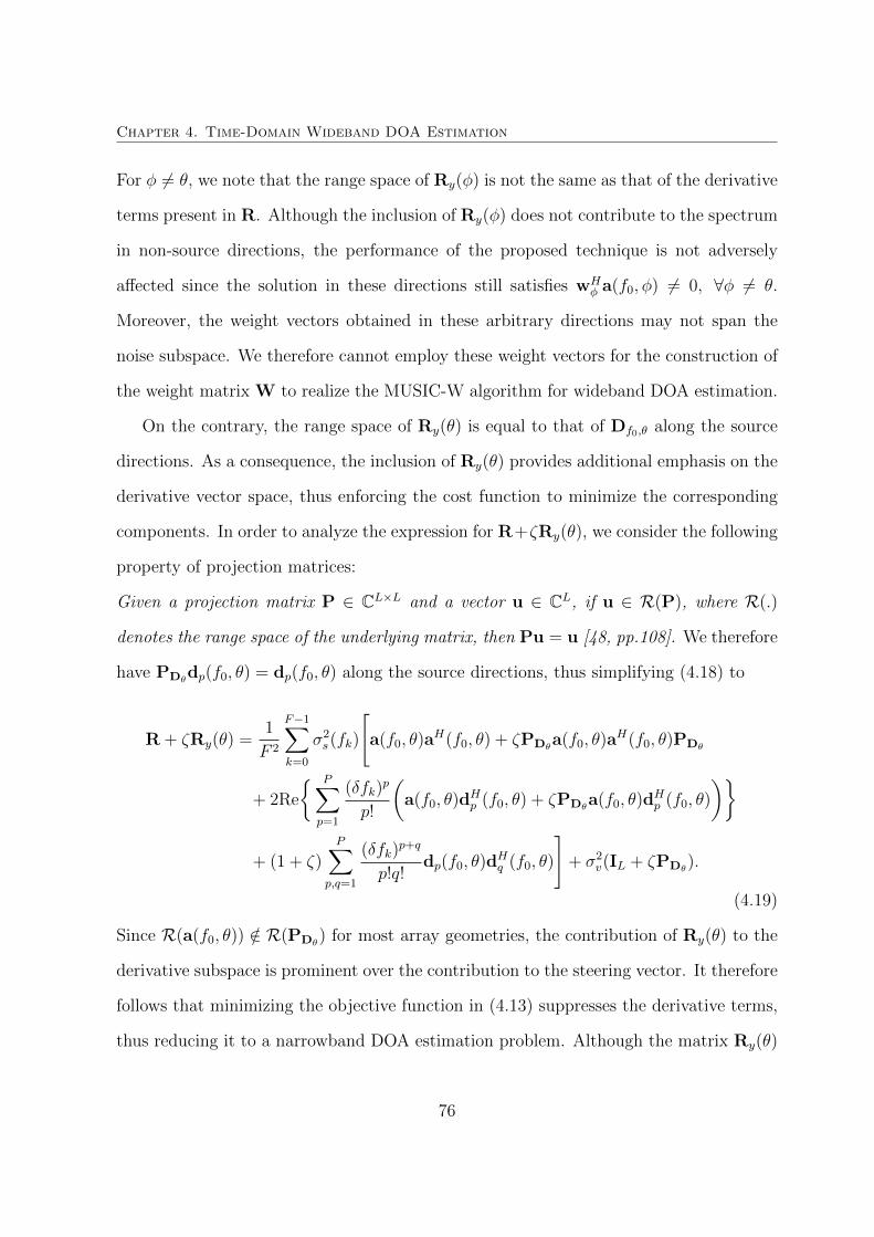
Chapter 4. Time-Domain Wideband DOA Estimation
For φ 6= θ, we note that the range space of Ry(φ) is not the same as that of the derivative
terms present in R. Although the inclusion of Ry(φ) does not contribute to the spectrum
in non-source directions, the performance of the proposed technique is not adversely
affected since the solution in these directions still satisfies wHφ a(f0, φ) 6= 0, ∀φ 6= θ.
Moreover, the weight vectors obtained in these arbitrary directions may not span the
noise subspace. We therefore cannot employ these weight vectors for the construction of
the weight matrix W to realize the MUSIC-W algorithm for wideband DOA estimation.
On the contrary, the range space of Ry(θ) is equal to that of Df0,θ along the source
directions. As a consequence, the inclusion of Ry(θ) provides additional emphasis on the
derivative vector space, thus enforcing the cost function to minimize the corresponding
components. In order to analyze the expression for R+ζRy(θ), we consider the following
property of projection matrices:
Given a projection matrix P ∈ CL×L and a vector u ∈ CL, if u ∈ R(P), where R(.)
denotes the range space of the underlying matrix, then Pu = u [48, pp.108]. We therefore
have PDθdp(f0, θ) = dp(f0, θ) along the source directions, thus simplifying (4.18) to
R + ζRy(θ) =1
F 2
F−1∑k=0
σ2s(fk)
[a(f0, θ)a
H(f0, θ) + ζPDθa(f0, θ)a
H(f0, θ)PDθ
+ 2Re
{ P∑p=1
(δfk)p
p!
(a(f0, θ)d
Hp (f0, θ) + ζPDθ
a(f0, θ)dHp (f0, θ)
)}
+ (1 + ζ)P∑
p,q=1
(δfk)p+q
p!q!dp(f0, θ)d
Hq (f0, θ)
]+ σ2
v(IL + ζPDθ).
(4.19)
Since R(a(f0, θ)) /∈ R(PDθ) for most array geometries, the contribution of Ry(θ) to the
derivative subspace is prominent over the contribution to the steering vector. It therefore
follows that minimizing the objective function in (4.13) suppresses the derivative terms,
thus reducing it to a narrowband DOA estimation problem. Although the matrix Ry(θ)
76
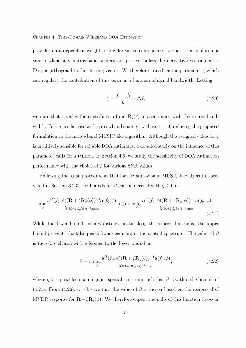
Chapter 4. Time-Domain Wideband DOA Estimation
provides data dependent weight to the derivative components, we note that it does not
vanish when only narrowband sources are present unless the derivative vector matrix
Df0,θ is orthogonal to the steering vector. We therefore introduce the parameter ζ which
can regulate the contribution of this term as a function of signal bandwidth. Letting
ζ =fu − fl
fc
= ∆f, (4.20)
we note that ζ scales the contribution from Ry(θ) in accordance with the source band-
width. For a specific case with narrowband sources, we have ζ = 0, reducing the proposed
formulation to the narrowband MUSIC-like algorithm. Although the assigned value for ζ
is intuitively sensible for reliable DOA estimates, a detailed study on the influence of this
parameter calls for attention. In Section 4.5, we study the sensitivity of DOA estimation
performance with the choice of ζ for various SNR values.
Following the same procedure as that for the narrowband MUSIC-like algorithm pro-
vided in Section 3.2.3, the bounds for β can be derived with ζ ≥ 0 as
minφ
aH(f0, φ)(R + ζRy(φ))−1a(f0, φ)
χ(R+ζRy(φ))−1,max
< β < maxφ
aH(f0, φ)(R + ζRy(φ))−1a(f0, φ)
χ(R+ζRy(φ))−1,max
.
(4.21)
While the lower bound ensures distinct peaks along the source directions, the upper
bound prevents the false peaks from occurring in the spatial spectrum. The value of β
is therefore chosen with reference to the lower bound as
β = η minφ
aH(f0, φ)(R + ζRy(φ))−1a(f0, φ)
χ(R+ζRy(φ))−1,max
, (4.22)
where η > 1 provides unambiguous spatial spectrum such that β is within the bounds of
(4.21). From (4.22), we observe that the value of β is chosen based on the reciprocal of
MVDR response for R + ζRy(φ). We therefore expect the nulls of this function to occur
77
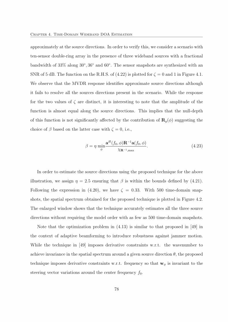
Chapter 4. Time-Domain Wideband DOA Estimation
approximately at the source directions. In order to verify this, we consider a scenario with
ten-sensor double-ring array in the presence of three wideband sources with a fractional
bandwidth of 33% along 30◦, 36◦ and 60◦. The sensor snapshots are synthesized with an
SNR of 5 dB. The function on the R.H.S. of (4.22) is plotted for ζ = 0 and 1 in Figure 4.1.
We observe that the MVDR response identifies approximate source directions although
it fails to resolve all the sources directions present in the scenario. While the response
for the two values of ζ are distinct, it is interesting to note that the amplitude of the
function is almost equal along the source directions. This implies that the null-depth
of this function is not significantly affected by the contribution of Ry(φ) suggesting the
choice of β based on the latter case with ζ = 0, i.e.,
β = η minφ
aH(f0, φ)R−1a(f0, φ)
χR−1,max
. (4.23)
In order to estimate the source directions using the proposed technique for the above
illustration, we assign η = 2.5 ensuring that β is within the bounds defined by (4.21).
Following the expression in (4.20), we have ζ = 0.33. With 500 time-domain snap-
shots, the spatial spectrum obtained for the proposed technique is plotted in Figure 4.2.
The enlarged window shows that the technique accurately estimates all the three source
directions without requiring the model order with as few as 500 time-domain snapshots.
Note that the optimization problem in (4.13) is similar to that proposed in [49] in
the context of adaptive beamforming to introduce robustness against jammer motion.
While the technique in [49] imposes derivative constraints w.r.t. the wavenumber to
achieve invariance in the spatial spectrum around a given source direction θ, the proposed
technique imposes derivative constraints w.r.t. frequency so that wφ is invariant to the
steering vector variations around the center frequency f0.
78

Chapter 4. Time-Domain Wideband DOA Estimation
0 50 100 150 200 250 300 35010
−4
10−3
10−2
10−1
100
φ (deg)
Am
plit
ud
e
Source directions
aH(f0,φ)(R+ζRy(φ))−1a(f0,φ)λ(R+ζRy(φ))−1,max
aH(f0,φ)R−1a(f0,φ)λR−1,max
Figure 4.1: Plot of aH(f0,φ)(R+ζRy(φ))−1a(f0,φ)
χ(R+ζRy(φ))−1,maxand aH(f0,φ)R−1a(f0,φ)
χR−1,maxin the presence of three
sources.
4.3.3 Computational Complexity
Evaluating the precise computational complexity for the proposed technique involves the
computation of the steering vector derivatives, matrix multiplication and solving a GEV
problem for each direction. With steering vector derivatives independent of data, the
run-time computational load can be reduced significantly with a look-up table of values
evaluated apriori. Therefore, solving GEV in each direction is the only run-time compu-
tationally intensive task. An iterative algorithm to realize generalized eigen decompo-
sition with a computational complexity of O(L2) has been proposed in [46]. Including
the computation cost for matrix inversion and maximum eigenvalue of R−1 required for
evaluating β (which together consumes O(L3) +O(L2)), the total computational cost of
the proposed technique is O(L3) + (Ntot + 1)O(L2), where Ntot is the number of search
directions.
79

Chapter 4. Time-Domain Wideband DOA Estimation
0 100 200 3000
5
10
15
20
25
30
35
40
45
50
Scan direction, (deg)
P(
), d
B
30 40 50 6010
20
30
40
50
Figure 4.2: Illustrative spatial spectrum of the proposed technique.
Besides ignoring the computational cost involved in the estimation of the signal sub-
space dimension, the BFW-MUSIC algorithm requires the inversion of a D ×D matrix
(D = dim(Es) + P ) in each direction resulting in a total cost of NtotO(D3). Although
D < L, the third-degree complexity indicates an increase in complexity with increasing
signal subspace dimension. DOA estimation using the TOPS algorithm requires an eigen
decomposition of the L × L autocorrelation matrix at each frequency bin, followed by
an eigen decomposition of a smaller P × P matrix in each direction. This results in a
total computational complexity of NbinsO(L2) + NtotO(P 2), where Nbins is the number
of frequency bins used. This is again a conservative measure without considering the
computations required for estimating the model order. While a single SVD is required
to be solved by the CSSM technique for DOA estimation, the process of finding the fo-
cussing matrices requires an L × L matrix SVD in each frequency bin of consideration.
Although this technique is computationally less intensive, it additionally requires an ini-
80

Chapter 4. Time-Domain Wideband DOA Estimation
tial estimate of the source directions obtained from another technique. Considering the
complexity of the model-order estimation techniques and the prerequisites required for
the CSSM algorithm, the proposed technique has comparable computational cost with
existing subspace-based techniques.
4.3.4 The {f, φ} Ambiguity
The steering vector in the context of narrowband DOA estimation is a function of only the
source direction since all the sources are assumed to be operating at the same frequency.
For wideband source scenario, however, the steering vector is a function of frequency and
direction. A combined processing of data across frequencies gives rise to an ambiguity
over the {f, φ} domain for some array configurations as reported in [30]. In order to
understand this ambiguity, consider a ULA where, the steering vector is given by
a(f, φ) =[1 e2πfτφ . . . e2πf(L−1)τφ ]T
=[1 e2πfdc
cosφ . . . e(L−1)2πf dc
cosφ]T .
(4.24)
From the argument of each element in the steering vector, we note that a few combinations
of frequency-direction pairs satisfy
(f + δf)τφ = f(τφ+δφ) (4.25)
over the azimuth range. Along these directions, the steering vectors a(f + δf, φ) and
a(f, φ + δφ) are indistinguishable, resulting in an ambiguity. We therefore observe false
peaks in some non-source directions for the proposed technique which exploits monotonic-
ity of steering vector across frequency. Although the use of 2−D array configurations
such as double-ring array can resolve this ambiguity, the technique cannot provide reli-
able estimates with primitive 1−D arrays. In order to resolve this problem we construct
81
Chapter 4. Time-Domain Wideband DOA Estimation
spatio-temporal observation vectors using D delays at the sensor outputs as suggested
in [30]. The number of taps D which introduces a temporal delay of TD is chosen such
that the product [ω × TD] mod 2π is unambiguous over all signal frequencies ω within
the observation bandwidth. The number of delays D can however be relaxed with the
choice of appropriate array configuration which ensures unambiguous [ω.TD] mod 2π
product [30].
For an L−sensor array, the time-domain snapshots x(n) are used to construct spatio-
temporal snapshots with D−tap delays as
x(n) =[xT (n) xT (n− 1) . . . xT (n−D)
]T. (4.26)
While existing subspace-based techniques can be employed for DOA estimation with
these snapshots, the broadband signal subspace dimension has to be determined based
on the observed source time-bandwidth product [30]. This product, and hence the signal
subspace dimension, varies with the scenario rather than the actual number of sources
present in the scenario. Alternatively, with the array manifold approximation discussed
in Section 4.2, we employ the MUSIC-like formulation to resolve the source directions
without estimating the model order. The array covariance matrix corresponding to the
spatio-temporal snapshots x(n) is given by
R = E{x(n)xH(n)}
≈ 1
F 2
[A(f0,Θ)
{ F−1∑k=0
Rss(fk)}
AH(f0,Θ) + 2F−1∑k=0
Re{ P∑p=1
(δfk)p
p!A(f0,Θ)Rss(fk)D
Hp (Θ)
}+
F−1∑k=0
P∑p,q=1
(δfk)p+q
p!q!Dp(Θ)Rss(fk)D
Hq (Θ)
]+ σ2
vIL,
(4.27)
82

Chapter 4. Time-Domain Wideband DOA Estimation
0 50 100 150-60
-50
-40
-30
-20
-10
0
Scan direction, (deg)
P(
) (dB
)
(b)
0 50 100 150-50
-45
-40
-35
-30
-25
-20
-15
-10
-5
0
Scan direction, (deg)
P(
) (dB
)(a)
Figure 4.3: Performance of the proposed technique under the {f, φ} ambiguity at anSNR of 5 dB (a) without time delay taps, (b) with D = 3 time delay taps.
where the matrix A(f0,Θ) consists of DL−dimensional steering vectors constructed as
a(f, θ) = [1, e2πfTs . . . , e2πf(D−1)Ts ]T ⊗ a(f, θ), (4.28)
with Ts denoting the time-delay between the temporal samples and ⊗ denotes the Kro-
necker product. The columns of D(f0,Θ) are obtained by the P derivatives of a(f, θ).
Employing the proposed technique on the spatio-temporal snapshots with the steer-
ing vector given in (4.28), the spatial spectrum is expected to provide distinct peaks
along the source directions for any array configuration. In order to demonstrate this,
we consider a ULA with five sensors and a source scenario with two wideband sources
from 50◦ and 70◦ having a normalized bandwidth of 0.1 and centered at fc = 0.3. The
spatio-temporal snapshots x(n) are synthesized at an SNR of 5 dB with a tap delay line
of D = 3. In Figure 4.3(a), the spatial spectrum of the proposed technique without any
time-delay taps is plotted. We note that the technique fails to estimate accurate source
83
Chapter 4. Time-Domain Wideband DOA Estimation
directions employing only the spatial snapshots. Furthermore, an ambiguous false peak
is observed in a non-source direction which satisfies the condition in (4.25). Figure 4.3(b)
shows the spatial spectrum when spatio-temporal structure is employed for DOA esti-
mation. It is observed that the technique resolves the ambiguity in identifying the true
source directions. Besides resolving the ambiguity, the incorporation of tap-delay line
increases the degrees-of-freedom, thus improving the DOA estimation accuracy at the
cost of increased computation complexity.
4.4 Derivation of the Cramer-Rao Lower Bound (CRLB)
The Cramer-Rao bound provides a lower bound on the estimation variance of a parameter
θ. If we have a vector of parameters Θ, the covariance matrix of estimation errors for
any unbiased estimate is bound by
C(Θ) ≥ CCR(Θ) , J−1, (4.29)
where CCR(Θ) denotes the CRLB for the covariance matrix which is equal to the inverse
of the Fisher’s information matrix (FIM) J.
For an L−element array, if each snapshot x follows a zero-mean complex Gaussian
random vector parameterized by Θ, the probability density function is given by
px|Θ(x) =1
det[πCx(Θ)]exp
{− xHC−1
x (Θ)x}, (4.30)
where Cx(Θ) is the covariance matrix of x. If we assume that the successive N snapshots
84

Chapter 4. Time-Domain Wideband DOA Estimation
are statistically independent, the log-likelihood function is given by
Lx(Θ) =N∑i=1
ln pxi|Θ(xi). (4.31)
The elements of the FIM are then evaluated as
Jij , E[∂Lx(Θ)
∂θi.∂Lx(Θ)
∂θj
]= E
[∂2Lx(Θ)
∂θi∂θj
], (4.32)
Exercising ergodicity, the covariance matrix of sensor snapshots R can be estimated using
the temporal snapshots. After simplifying (4.32), the FIM for Θ is given by
Jij = NTr
(∂R
∂θiR−1∂R
∂θjR−1
), ∀, i, j = 1, ...,M. (4.33)
For detailed derivation of (4.33), please refer to [2, Chap. 8].
For the time-domain wideband signal model with array manifold approximation given
in (4.4), the covariance matrix R is given by (4.10). The partial derivative of R w.r.t.
each parameter is given by
∂R
∂θi=
1
F 2
F−1∑k=0
[A(f0,Θ)Rss(fk)A
H(f0,Θ) + A(f0,Θ)Rss(fk)AH(f0,Θ)
+ 2Re{ P∑p=1
(δfk)p
p!
(A(f0,Θ)Rss(fk)D
Hp (f0,Θ) + A(f0,Θ)Rss(fk)D
Hp (f0,Θ)
)}+
P∑p,q=1
(δfk)p+q
p!q!
(Dp(f0,Θ)Rss(fk)D
Hq (f0,Θ) + Dp(f0,Θ)Rss(fk)D
Hq (f0,Θ)
)],
(4.34)
where A(f0,Θ) = ∂∂θi
A(f0,Θ) and Dp(f0,Θ) = ∂p+1
∂θifpA(f0,Θ). The noise variance at each
85
Chapter 4. Time-Domain Wideband DOA Estimation
frequency bin is estimated as σ2v(fk) as
σ2v(fk) =
1
L−M trace{
IL −A(fk,Θ)(AH(fk,Θ)A(fk,Θ)
)−1AH(fk,Θ)
}. (4.35)
The source covariance matrix can then be estimated as
Rss(fk) =(AH(fk,Θ)A(fk,Θ)
)−1AH(fk,Θ)
(R(fk)−σ2
v(fk)IL)A(fk,Θ)
(AH(fk,Θ)A(fk,Θ)
)−1,
(4.36)
where R(fk) is the array covariance matrix estimated from the sensor snapshots at fre-
quency fk. With the source covariance matrix estimated, the FIM, and hence the CRB
can be estimated by substituting (4.34) into (4.33).
4.5 Simulation Results and Discussions
In this section, the performance of the proposed technique is evaluated using Monte-
Carlo simulations. For all the simulations, we employ a double-ring array of ten elements
(L = 10) shown in Figure 4.4 with the array phase center coinciding with the origin of
the coordinate system. Since this array geometry does not exhibit the {f, φ} ambiguity
unlike the ULA, we use D = 0 tap delays. The source azimuths are measured from
the horizontal x-axis. Despite the radius of the two rings being greater than λmin/2,
the farfield planar wavefront from any source direction is sampled by a set of sensors
complying with the λmin/2 phase delay, thus avoiding any source direction ambiguity
due to spatial aliasing. The wideband sources are generated as a sum of sinusoids with
random phase and magnitude within the bandwidth,
s(t) =
Bbw∑i=1
aiexp{(2πfit+ ci(t))}, (4.37)
86
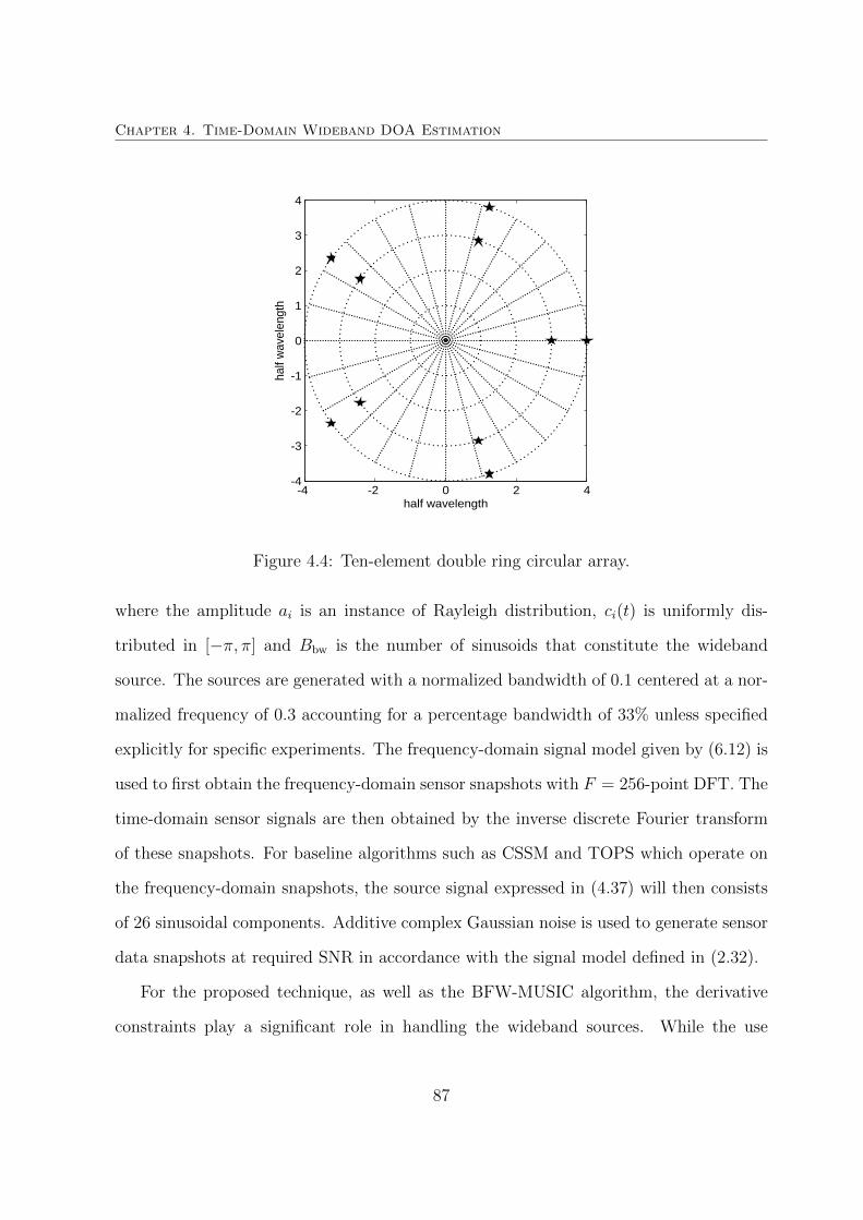
Chapter 4. Time-Domain Wideband DOA Estimation
-4 -2 0 2 4-4
-3
-2
-1
0
1
2
3
4
half
wav
elen
gth
half wavelength
Figure 4.4: Ten-element double ring circular array.
where the amplitude ai is an instance of Rayleigh distribution, ci(t) is uniformly dis-
tributed in [−π, π] and Bbw is the number of sinusoids that constitute the wideband
source. The sources are generated with a normalized bandwidth of 0.1 centered at a nor-
malized frequency of 0.3 accounting for a percentage bandwidth of 33% unless specified
explicitly for specific experiments. The frequency-domain signal model given by (6.12) is
used to first obtain the frequency-domain sensor snapshots with F = 256-point DFT. The
time-domain sensor signals are then obtained by the inverse discrete Fourier transform
of these snapshots. For baseline algorithms such as CSSM and TOPS which operate on
the frequency-domain snapshots, the source signal expressed in (4.37) will then consists
of 26 sinusoidal components. Additive complex Gaussian noise is used to generate sensor
data snapshots at required SNR in accordance with the signal model defined in (2.32).
For the proposed technique, as well as the BFW-MUSIC algorithm, the derivative
constraints play a significant role in handling the wideband sources. While the use
87

Chapter 4. Time-Domain Wideband DOA Estimation
0 20 40 60 80 100 120 140 160 180-40
-30
-20
-10
0
Scan direction, (deg)
Pow
er
(dB
)
(a) BFW-MUSIC algorithm
0 20 40 60 80 100 120 140 160 180-50
-40
-30
-20
-10
0
Scan direction, (deg)
Pow
er
(dB
)
(b) Proposed TD-DOA
P = 1P = 2P = 3P = 4
P = 1P = 2P = 3P = 4
Figure 4.5: Spatial spectra with different derivative orders P at an SNR of 5 dB for (a)BFW-MUSIC, (b) proposed technique.
of higher-order derivative constraints is expected to completely suppress the derivative
terms in (4.10), the optimization problem of BFW-MUSIC and the proposed technique
restricts the use of large number of derivative constraints due to the limited degrees
of freedom available. This is observed with a simulation consisting of three wideband
sources at 50◦, 70◦ and 80◦. With 500 time-domain snapshots at an SNR of 5 dB,
the spatial spectra for both the techniques are plotted for different derivative orders
P in Figure 4.5. In Figure 4.5(a), we note that the BFW-MUSIC algorithm provides
reliable DOA estimates by incorporating derivative constraints. However, an increase in
88
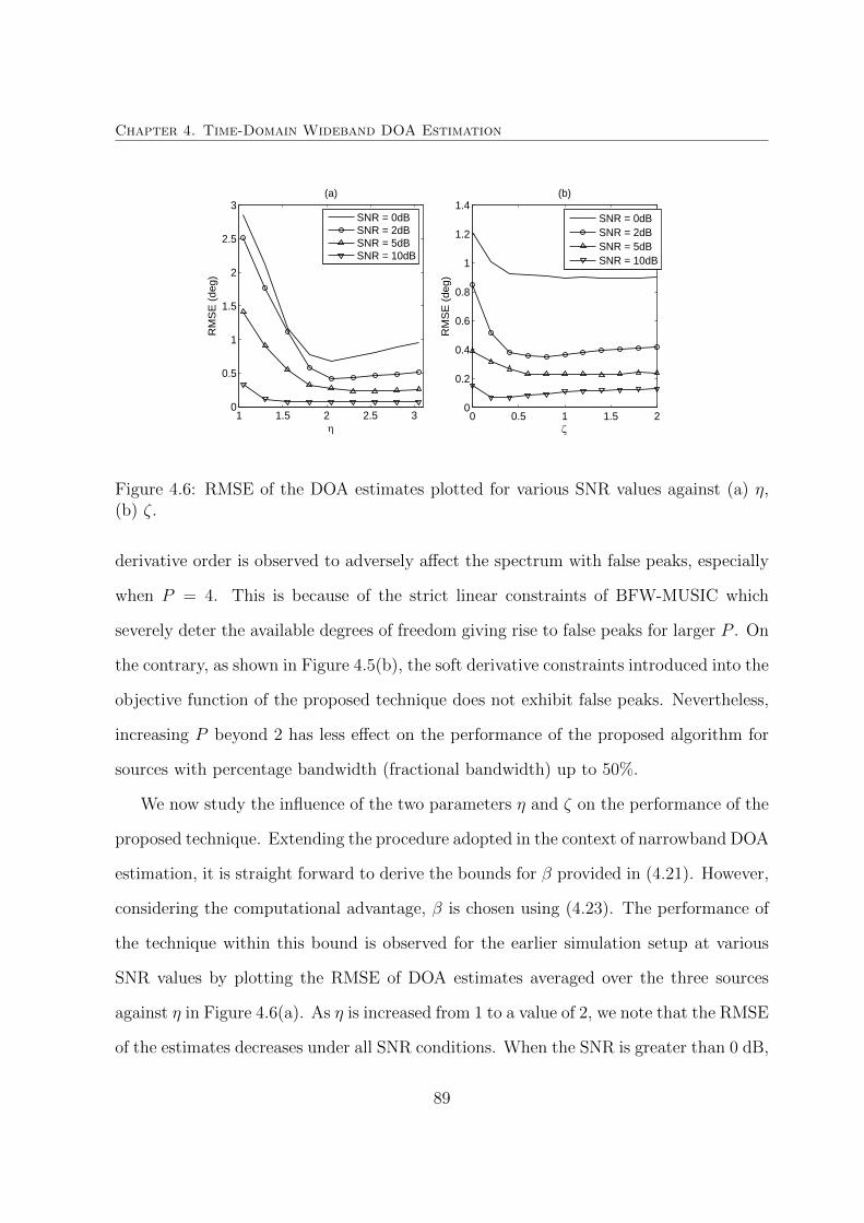
Chapter 4. Time-Domain Wideband DOA Estimation
1 1.5 2 2.5 30
0.5
1
1.5
2
2.5
3R
MS
E (
deg)
(a)
SNR = 0dBSNR = 2dBSNR = 5dBSNR = 10dB
0 0.5 1 1.5 20
0.2
0.4
0.6
0.8
1
1.2
1.4
RM
SE
(deg)
(b)
SNR = 0dBSNR = 2dBSNR = 5dBSNR = 10dB
Figure 4.6: RMSE of the DOA estimates plotted for various SNR values against (a) η,(b) ζ.
derivative order is observed to adversely affect the spectrum with false peaks, especially
when P = 4. This is because of the strict linear constraints of BFW-MUSIC which
severely deter the available degrees of freedom giving rise to false peaks for larger P . On
the contrary, as shown in Figure 4.5(b), the soft derivative constraints introduced into the
objective function of the proposed technique does not exhibit false peaks. Nevertheless,
increasing P beyond 2 has less effect on the performance of the proposed algorithm for
sources with percentage bandwidth (fractional bandwidth) up to 50%.
We now study the influence of the two parameters η and ζ on the performance of the
proposed technique. Extending the procedure adopted in the context of narrowband DOA
estimation, it is straight forward to derive the bounds for β provided in (4.21). However,
considering the computational advantage, β is chosen using (4.23). The performance of
the technique within this bound is observed for the earlier simulation setup at various
SNR values by plotting the RMSE of DOA estimates averaged over the three sources
against η in Figure 4.6(a). As η is increased from 1 to a value of 2, we note that the RMSE
of the estimates decreases under all SNR conditions. When the SNR is greater than 0 dB,
89

Chapter 4. Time-Domain Wideband DOA Estimation
further increase in η beyond 2 is observed to have less significance on the estimation
accuracy. However, as η guides β towards its upper bound, the spatial spectrum will be
affected with false peaks due to the relaxation of the constraint explained while deriving
the bounds for β in Section 3.2.3. When SNR≤ 0, the RMSE gradually increases with
increasing η. We therefore employ η = 2 for all the simulations.
With this choice for η, we observe the effect of ζ on the DOA estimates for the same
simulation setup. Figure 4.6(b) shows the RMSE of DOA estimates plotted against ζ for
various SNR values. We note that the RMSE for DOA estimates is large for ζ < 0.5. This
is due to the insufficient suppression of derivative components in R. For ζ ≥ 0.5, which
is equal to the fractional bandwidth BW/fc the estimation accuracy is not significantly
affected.
Frequency-domain techniques such as CSSM and TOPS require the estimation of
covariance matrix at each frequency bin within the signal bandwidth. For reliable DOA
estimation, sufficient frequency-domain snapshots are essential for the covariance matrix
estimation in each frequency bin. If J denotes the number of frequency-domain snapshots
used for DOA estimation, the corresponding temporal snapshots N = JF required is
significantly large. Since the proposed technique operates on time-domain snapshots, the
covariance matrix R encompasses information from the entire signal bandwidth. This
simultaneous processing across the signal bandwidth reduces the number of snapshots
required for DOA estimation. We first evaluate the proposed technique in comparison
with the BFW-MUSIC algorithm employing reduced number of temporal snapshots,
followed by which, the technique is compared with other baseline algorithms using larger
snapshots.
Three wideband sources with a percentage bandwidth of 33% are situated at 40◦,
50◦ and 70◦. Employing 1500 time-domain snapshots for DOA estimation, the RMSE
of direction estimates are plotted against SNR in Figure 4.7. The performance of the
90

Chapter 4. Time-Domain Wideband DOA Estimation
proposed technique with P = 1 and P = 2 are shown with the BFW-MUSIC algorithm
being used as a baseline algorithm. Since the signal subspace dimension of R includes
additional terms in (4.10), the BFW-MUSIC algorithm is implemented with dim{Es} =
M + 2. Linear derivative constraints of up to P = 2 are used to obtain the spatial
spectrum of BFW-MUSIC. The RMSE of DOA estimates is plotted against SNR for the
two techniques in Figure 4.7 along with the square root of the Cramer-Rao lower bound
(sqrtCRB).
With prior knowledge of the approximate signal subspace dimension and the strict
linear constraints, BFW-MUSIC is observed to perform better when the SNR is low. It
is important to note that an inappropriate signal subspace dimension adversely affects
the performance of this algorithm which is not shown in the figure. On the contrary, the
estimation accuracy of the proposed technique without using prior information of the
signal subspace dimension, is observed to have marginally lower performance at lower
SNR conditions. However, as the SNR is increased we note that the proposed technique
outperforms the BFW-MUSIC algorithm. This is because, at higher SNR values, the
noise subspace is clearly segregated from the composite subspace in the covariance matrix,
which enables one to direct the weight vector to reside in the noise subspace. In such
scenario, the data dependent suppression of derivative components will be more effective
than the linear constraints of the BFW-MUSIC algorithm. The improvement in the
performance for P = 2 over P = 1 reflects the importance of including Ry(φ) and its
order. Knowledge of the source covariance matrix used in evaluating the CRLB explains
the difference between the performance of the two techniques and the CRLB.
We now investigate the estimation performance as a function of the number of snap-
shots that is used to construct R and Ry(θ). Fixing the SNR at 5 dB for the same
source-sensor configuration as the previous simulation, source directions are estimated
using the proposed technique and the BFW-MUSIC algorithm. In Figure 4.8, we note the
91

Chapter 4. Time-Domain Wideband DOA Estimation
estimation accuracy of both the techniques increases with the number of snapshots. The
RMSE of DOA estimates obtained by the proposed technique approaches that of BFW-
MUSIC and outperforms the latter when the number of snapshots is increased further.
While the provided signal subspace dimension and the strict linear derivative constraints
aid to have relatively better performance for BFW-MUSIC with limited number of snap-
shots, the improvement in the estimation of R with larger number of snapshots has less
impact on its solution.
The capability of the proposed technique to resolve two closely situated sources is now
studied for two wideband sources with a percentage bandwidth of 50%. The probability
of resolution is studied with increase in SNR for 5◦, 7◦ and 9◦ of angular separation
between the two sources in Figure 4.9. The number of snapshots used is 1000. When
the sources are closely-situated, A(f0,Θ) and Dp(Θ) are highly ill-conditioned. In the
presence of large additive noise σ2v and the approximation errors, the two sources are
indistinguishable by the proposed technique. Therefore, we note that larger SNR is
required to resolve the two sources when they are separated by 5◦. When the angular
separation between the sources is increased to 7◦ and 9◦, the technique can resolve the
source directions at much smaller SNR.
In order to compare the performance of the proposed technique with frequency do-
main techniques such as CSSM and TOPS, we study the RMSE of the source DOA
estimates. The number of frequency bins used for DOA estimation with TOPS is equal
to the source bandwidth. The frequency-domain snapshots are obtained with a 256-point
FFT performed on the sensor snapshots. While J = 25 frequency-domain snapshots are
used for the TOPS algorithm, equivalent number of time-domain snapshots 256 × 25
is used for the proposed technique. Three sources with 50% bandwidth are positioned
at 12◦, 40◦ and 48◦. Figure 4.10 shows the RMSE of the source estimates for all the
techniques averaged over 200 trials along with the CRLB (sqrtCRB). Among all the
92

Chapter 4. Time-Domain Wideband DOA Estimation
compared techniques, CSSM is observed to have the best performance at low SNR condi-
tions. However, the solution is highly susceptible to the initial estimates provided to the
technique. Moreover, the performance saturates with the increase in SNR as the array
manifold fitting error cannot be eliminated with an increase in SNR. The TOPS algo-
rithm is observed to have the worst performance at lower SNR conditions and the plots
shown in Figure 4.10 are consistent with the observation made in [41]. The performance
of TOPS is comparable with other techniques only at mid and high SNR ranges. At
lower SNR conditions, the BFW-MUSIC algorithm shows better performance over the
proposed technique with the support of the approximate signal subspace dimension and
the linear derivative constraints. Nevertheless, its performance does not improve signifi-
cantly with the SNR. In contrast, the estimation performance of the proposed technique
improves with SNR compared to other techniques. In view of the insensitivity to the in-
correct model order estimated at lower SNR conditions, the performance of the proposed
technique is acceptable.
Figure 4.11 shows the ability of all the techniques under comparison to resolve the
three source directions in the earlier source scenario. Each source is considered to be
resolved when the algorithm provides a significant peak within the spatial region [θi −
∆θ, θi + ∆θ], where ∆θ = min{θi − θj}/2,∀i, j, i 6= j ∈ M . The CSSM and BFW-
MUSIC algorithms are observed to have good resolution capability with the advantage of
partial information of the model order. Since the distinction between the noise and signal
subspace eigenvalues is not significant at low SNR conditions, the proposed technique is
observed to have marginally lower resolution capability than the BFW-MUSIC algorithm.
As expected, the TOPS algorithm estimate source directions only when the SNR is
significantly high.
93

Chapter 4. Time-Domain Wideband DOA Estimation
4.6 Conclusion
In this chapter, a new approach to coherently process the wideband data across the signal
bandwidth using the Taylor series expansion of the array manifold w.r.t. frequency has
been proposed. The covariance matrix obtained from the time-domain signal model has
been identified to have a coherently averaged narrowband component which preserves
the DOA information along with the additional derivative components. Exploiting this
observation, a new DOA estimation technique has been proposed which suppresses the
unnecessary derivative terms before estimating the source directions using the MUSIC-
like structure. The effective suppression of these terms by the proposed technique has
been analyzed in detail. Being insensitive to the estimated model order, the performance
of this technique has been shown to be comparable with existing techniques through
simulations.
94

Chapter 4. Time-Domain Wideband DOA Estimation
-10 -5 0 5 10 15 20 25 30
100
10-1
10-2
10-3
RM
SE
(de
g)
SNR (dB)
(a) Source 1
-10 -5 0 5 10 15 20 25 30
100
10-1
10-2
10-3
RM
SE
(de
g)
SNR (dB)
(b) Source 2
-10 -5 0 5 10 15 20 25 30
100
10-1
10-2
10-3
RM
SE
(de
g)
SNR (dB)
(c) Source 3
sqrtCRB
Proposed TD-DOA, P=1
sqrtCRB
Proposed TD-DOA, P=1
sqrtCRBBFW-MUSIC
Proposed TD-DOA, P=1
BFW-MUSIC
BFW-MUSICProposed
TD-DOA, P=2
Proposed TD-DOA, P=2
Proposed TD-DOA, P=2
Figure 4.7: RMSE of DOA estimates against SNR with 1500 time-domain snapshots.
95

Chapter 4. Time-Domain Wideband DOA Estimation
1000 2000 3000 4000 5000 6000 7000 8000 9000 1000010
-3
10-2
10-1
100
RM
SE
(de
g)
Number of snapshots
(a) Source 1
1000 2000 3000 4000 5000 6000 7000 8000 9000 1000010
-3
10-2
10-1
100
RM
SE
(de
g)
Number of snapshots
(b) Source 2
1000 2000 3000 4000 5000 6000 7000 8000 9000 10000
10-2
100
RM
SE
(de
g)
Number of snapshots
(c)Source 3
sqrt(CRB)
sqrt(CRB)
sqrt(CRB)
Proposed TD-DOA
Proposed TD-DOA
BFW-MUSIC
BFW-MUSIC
Proposed TD-DOA
BFW-MUSIC
Figure 4.8: RMSE of DOA estimates as a function of the number of snapshots in com-parison with the BFW-MUSIC algorithm. The snapshots are obtained at 5 dB SNR.
96

Chapter 4. Time-Domain Wideband DOA Estimation
-30 -20 -10 0 10 20 300
0.2
0.4
0.6
0.8
1
SNR (dB)
Pro
babi
lity
of R
esol
utio
n
=5
=9
=7
Figure 4.9: Probability of resolving two sources with angular separations ∆θ = 5◦,∆θ = 7◦ and ∆θ = 9◦.
97

Chapter 4. Time-Domain Wideband DOA Estimation
-10 -5 0 5 10 15 20
100
10-3
10-1
10-2
RM
SE
(de
g)
SNR (dB)
(a) Source 1
-10 -5 0 5 10 15 2010
-4
10-2
100
RM
SE
(de
g)
SNR (dB)
(b) Source 2
-10 -5 0 5 10 15 20
10-2
100
10-1
10-3
RM
SE
(de
g)
SNR (dB)
(c) Source 3
-10 -5 0 5 10 15 20
10-2
100
10-1
10-3
RM
SE
(de
g)
SNR (dB)
(b) Source 2
TOPS
CSSMBFW-MUSIC
sqrtCRB
CSSM
sqrtCRB
BFW-MUSIC
ProposedTD-DOACSSM
TOPS
sqrtCRB
BFW-MUSIC
ProposedTD-DOA
ProposedTD-DOA
TOPS
Figure 4.10: RMSE of DOA estimates against SNR in comparison with the CSSM, TOPSand BFW-MUSIC algorithms when the sources are situated at 12◦, 40◦ and 48◦.
98

Chapter 4. Time-Domain Wideband DOA Estimation
-20 -15 -10 -5 0 5 10 15 20 250
0.1
0.2
0.3
0.4
0.5
0.6
0.7
0.8
0.9
1
Pro
babi
lity
of R
esol
utio
n
SNR (dB)
ProposedTD-DOA
BFW-MUSIC
CSSM
TOPS
Figure 4.11: The probability of resolving all the three sources by CSSM, TOPS, BFW-MUSIC and the proposed technique.
99

Chapter 5
Derivative-Constrained
Frequency-Domain Wideband DOA
Estimation
5.1 Introduction
In Chapter 4, a time-domain DOA estimation technique was presented which estimates
wideband source directions with relatively reduced number of time-domain snapshots.
The use of MUSIC-like formulation provides distinct peaks in the spatial spectrum of the
technique without estimating the number of sources. For a wideband source scenario with
center frequency fc, if the maximum frequency deviation is defined as δfmax = fu − fc
such that the bandwidth is equal to fu−fl = 2δfmax, the underlying idea is to express the
steering vector at a frequency f within the signal bandwidth as a Taylor series expansion
with respect to the reference frequency f0 as
a(f, θ, P ) ≈ a(f0, θ) +P∑p=1
(δf)p
p!
∂p
∂f pa(f, θ)
∣∣∣∣f=f0
. (5.1)
100
Chapter 5. Derivative-Constrained Frequency-Domain Wideband DOA Estimation
However, the consequence of truncating the Taylor series expansion (TSE) up to an order
of P introduces approximation error as the frequency deviation δf increases. In order to
observe the effect of P th-order approximation and the frequency deviation, we evaluate
the approximation error e = ‖a(f, θ)−a(f, θ, P )‖2 in an arbitrary direction for the double-
ring array shown in Figure 4.4. A frequency deviation of δf = 0.04 from a normalized
frequency of f0 = 0.3 corresponding to a percentage bandwidth of 2δf/f0 × 100 ≈ 27%
is used for the illustration. The approximation error is plotted against TSE order in
Figure 5.1(a). We note that the error is considerably low for P ≥ 2 indicating that a
P−ordered TSE is a good approximation. In the associated simulation, we study the
error in approximation as the steering vector deviates from f0. The error e is plotted
against δf for various orders of the Taylor series expansion in Figure 5.1(b). For P ≥ 2,
we note that the approximation error is acceptable up to δf = 0.04, or equivalently 27%
bandwidth, beyond which the error increases significantly. It can hence be inferred that
the error in approximation increases drastically when the fractional source bandwidth
is larger than 0.27 or 0.33. In such cases, the performance of the time-domain DOA
estimation (TD-DOA) technique proposed in Chapter 4 deteriorates considerably. In
order to observe this phenomenon, we study the estimation accuracy of this technique
with the source bandwidth with a simulation consisting of three wideband sources at
12◦, 50◦ and 60◦ using the double-ring array with L = 10 sensors. The RMSE of the
three DOA estimates are averaged and plotted against the fractional bandwidth of the
sources. With 1500 snapshots and an SNR of 5 dB, the RMSE of the sources are plotted
against the fractional bandwidth ∆f in Figure 5.2.
Although the estimation errors for different sources vary due to their spatial posi-
tions, we observe that the RMSE increases with an increase in the signal bandwidth.
This reflects the limitation of time-domain processing for a source scenario with large
bandwidth due to inaccurate approximation. In order to reduce this approximation error,
101

Chapter 5. Derivative-Constrained Frequency-Domain Wideband DOA Estimation
0 2 4 6 8 1010
−10
10−5
100
Derivative order, P
e=
‖a(f
,θ)−
a(f
,θ,P
)‖2
(a)
0.01 0.02 0.03 0.04 0.05 0.06 0.07 0.080
0.5
1
1.5
2
Normalized frequency deviation from the center frequency, δf
e=
‖a(f
,θ)−
a(f
,θ,P
)‖2
(b)
P=1P=2P=3P=4
Figure 5.1: Error in steering vector approximation using TSE against (a) derivative orderfor δf = 0.04, (b) δf for various values of P .
it is essential to regulate the signal bandwidth under consideration while constructing
the covariance matrix. Towards this, we translate the problem to the frequency domain
and redefine the signal model with array manifold approximation.
In the literature we have several frequency-domain techniques which have shown good
DOA estimation performance. While ISSM, and the more recent TOPS algorithm yield
accurate DOA estimates in uncorrelated source scenario, the CSSM, reviewed in Sec-
tion 2.3.2.2, can estimate DOA in the presence of completely correlated sources as well.
The coherent averaging of the array covariance matrix across the signal bandwidth re-
stores the effective rank of the source covariance matrix enabling the DOA estimation of
correlated sources. However, the performance of all these techniques are sensitive to the
estimated number of sources.
102

Chapter 5. Derivative-Constrained Frequency-Domain Wideband DOA Estimation
0.2 0.3 0.4 0.5 0.6 0.7 0.80
0.5
1
1.5
2
2.5
RM
SE
(de
g)
f
Source 2
Source 3
Source 1
Figure 5.2: RMSE of DOA estimates plotted against fractional bandwidth.
Since the coherently averaged covariance matrix Rcssm exhibits narrowband structure
with transformed noise covariance matrix Rv, statistical techniques such as MDL and
AIC have been suggested in [33] for model order estimation even in wideband source
scenario. The generalized eigenvalues of the matrix pencil {Rcssm,Rv} are subject to
either MDL or AIC for model order estimation. Although these techniques provide
reliable estimates under moderate SNR conditions, the performance is unreliable when
the number of frequency-domain snapshots is low either due to the inaccurate estimation
of the correlated noise covariance matrix or due to adverse source scenarios.
We verify this inaccuracy with a simulation example where we study the model order
estimated by MDL and AIC employing the generalized eigenvalues of {Rcssm,Rv} for
two source scenarios. In the first scenario, two wideband sources are situated at 40◦ and
48◦. For the second scenario, the sources are situated at 40◦ and 58◦. The two sources
are uncorrelated with each other and have a percentage bandwidth of 27%. The matrix
Rcssm is estimated using (2.44) with 10 frequency-domain snapshots. In order to observe
103

Chapter 5. Derivative-Constrained Frequency-Domain Wideband DOA Estimation
Figure 5.3: Performance of MDL and AIC techniques against SNR when J = 10frequency-domain snapshots are used.
the performance of existing model order estimation techniques, we study the ratio of
the true number of sources M to the estimated model order M . The ratio approaches
unity when the algorithm estimates correct model order. The ratio M/M is averaged
over 100 trials and plotted against SNR for the two source scenarios in Figure 5.3. For
the first scenario where the sources are closely situated, we note that the ratio for both
the algorithms decreases below 1 with the increase in SNR. This indicates that the two
algorithms over estimate the number of sources present in the scenario with the increase
in the SNR. When the two sources are widely-spaced, both the algorithms estimate
M accurately over specific SNR values and over estimate the number of sources when
the SNR is increased further due to the inaccurate estimation of the transformed noise
covariance matrix. The spatial spectrum of CSSM would therefore exhibit more number
of peaks than the true model order. Under adverse conditions, it is therefore a challenging
problem to accurately estimate the model order estimation in the context of wideband
104

Chapter 5. Derivative-Constrained Frequency-Domain Wideband DOA Estimation
sources.
While the time-domain wideband DOA estimation technique proposed in Chapter 4
provides accurate DOA estimation with unknown model order, it was observed that the
estimation accuracy of the algorithm deteriorates with an increase in the signal band-
width. In this chapter, we therefore translate the problem to the frequency domain where
the source bandwidth being processed can be regulated such that the array manifold Tay-
lor series approximation error is acceptable. We first redefine the frequency-domain signal
model with array manifold approximation in Section 5.2. Since the BFW-MUSIC algo-
rithm also relies on this approximation, we first present its extension to the frequency
domain in Section 5.3.1. However, this algorithm still depends on the estimated dimen-
sion of the signal subspace of the array covariance matrix. We then present the extension
of the proposed formulation for wideband DOA estimation in Chapter 4 over a regulated
signal bandwidth in Section 5.3.2. Although these algorithms provide accurate DOA
estimates, they do not use the DOA information present in the unused portion of source
bandwidth. We therefore present a multi-band DOA estimation approach by incoher-
ently combining the DOA spectra obtained over various subbands. The three techniques
discussed in Section 5.3 are evaluated in Section 5.4 using simulated experiments. The
conclusion and the performance advantage of the presented techniques are summarized
in Section 5.5.
5.2 Signal Model with Array Manifold Approxima-
tion
In Section 4.2, sensor snapshots in the time domain were modeled by introducing array
manifold approximation into the signal model. The inverse-DFT relation includes fre-
105
Chapter 5. Derivative-Constrained Frequency-Domain Wideband DOA Estimation
quency components corresponding to the entire source bandwidth. However, as observed
in the previous section, inclusion of components which are farther from the reference
frequency increases the Taylor series approximation error, yielding inaccurate results. In
order to regulate the signal bandwidth under consideration, we estimate wideband source
directions with an averaged covariance matrix obtained across a smaller frequency band.
In the frequency domain, the sensor snapshots at a given frequency are modeled as
shown in (2.32). Expressing the array manifold matrix A(f,Θ) in terms of the reference
frequency f0 with Taylor series approximation, the signal model at frequency fk is given
by
x(k, l) ≈(
A(f0,Θ) +P∑p=1
(δfk)p
p!
∂pA(f,Θ)
∂f p
∣∣∣∣f=f0
)s(k, l) + v(k, l). (5.2)
With this approximation, the spatial covariance matrix of the zero-mean snapshots x(k, l)
can be expressed as
R(fk) =E{x(k, l)xH(k, l)
}≈A(f0,Θ)Rss(fk)A
H(f0,Θ) + σ2v(fk)IL
+L∑p=1
(δfk)p
p!Re
[A(f0,Θ)Rss(fk)
∂p
∂f pAH(f,Θ)
∣∣∣∣f=f0
]
+P∑
p,q=1
(δfk)p+q
p!q!
∂p
∂f pA(f,Θ)
∣∣∣∣f=f0
Rss(fk)∂q
∂f qAH(f,Θ)
∣∣∣∣f=f0
,
(5.3)
where σ2v(fk) is the variance of additive uncorrelated sensor noise at frequency fk. We
first define a fractional bandwidth ∆fB corresponding to B + 1 frequency bins, with B
even, in the proximity of f0, over which a P th-order Taylor series approximates the array
manifold up to an acceptable error. An average covariance matrix across this bandwidth
can then be defined as
Rav =1
B + 1
f0+B/2∑fk=f0−B/2
R(fk). (5.4)
106
Chapter 5. Derivative-Constrained Frequency-Domain Wideband DOA Estimation
Defining the data matrix at each frequency fk as
X(k) =[x(k, 1), . . . ,x(k, J)
], (5.5)
where J is the number of frequency domain snapshots, the data matrices across the B+1
frequency bins are then concatenated to form
X =[X(−B/2), . . . ,X(B/2)
]∈ CL×J(B+1). (5.6)
The covariance matrix Rav can then be estimated as
Rav =1
J(B + 1)XXH . (5.7)
If the source spectrum is uncorrelated across frequency, i.e., E{s(k1, l)sH(k2, l)} = 0M ,∀f1 6=
f2 and the additive sensor noise is uncorrelated with sources, we have
Rav ≈1
B + 1
[A(f0,Θ)
{ k0+B/2∑k=k0−B/2
Rss(fk)
}AH(f0,Θ)
+ 2
k0+B/2∑k=k0−B/2
Re
{ P∑p=1
(δfk)p
p!A(f0,Θ)Rss(fk)D
Hp (Θ)
}
+
k0+B/2∑k=k0−B/2
P∑p,q=1
(δfk)p+q
p!q!Dp(Θ)Rss(fk)D
Hq (Θ) +
k0+B/2∑k=k0−B/2
σ2v(fk)IL
],
(5.8)
where Dp(Θ) is the pth-order derivative matrix defined in (4.9). The coherent summation
of Rss(fk) across the source bandwidth in the first term restores the rank of the effective
source covariance matrix when the sources are completely correlated. It is therefore pos-
sible to resolve coherent source directions when this covariance matrix is used for DOA
estimation. We note that the average covariance matrix Rav has a similar expression as
107

Chapter 5. Derivative-Constrained Frequency-Domain Wideband DOA Estimation
that of the time-domain covariance matrix R in (4.10) with a coherent narrowband com-
ponent and components with derivative terms. However, the signal bandwidth beyond
∆fB will have less impact on this matrix, and hence on the DOA estimation. For an
F−point DFT, the maximum frequency deviation from f0 is δfmax = B+12F
. With δfmax
known, the order of TSE necessary for A(f,Θ) to constrain the approximation error can
be chosen based on Figure 5.1(b).
5.3 Proposed DOA Estimation
As discussed in Section 1.2, a signal is classified as narrowband when the fractional
bandwidth ∆f << 0.1, in which case, the narrowband MUSIC-like algorithm or MUSIC-
W algorithm can be employed to estimate source directions. However, for ∆f ≥ 0.1,
the sources have to be considered as wideband in nature. When 0.1 < ∆f < 0.3, or
equivalently 0.015 < δf < 0.045, it was observed in Figure 5.1 that the approximation
error is not significant when the derivative order is restricted to P = 2. The TD-DOA
estimation technique proposed in Chapter 4 is well suited for such scenarios. For a source
scenario with ∆f > 0.3, the estimation error increases significantly due to the array
manifold approximation of order P = 2. We therefore need to restrict the processing
bandwidth to ∆f ≤ 0.3 for the specified derivative order. This can be accomplished with
the frequency-averaged covariance matrix Rav given by (5.8). Since the BFW-MUSIC
algorithm also relies on the concept of array manifold approximation, we first present
its extension to the frequency domain. While the derivative constraints can successfully
suppress the derivative components, the formulation requires the knowledge of the signal
subspace dimension of Rav. In order to circumvent the model order or the signal subspace
dimension, we then present the extension of the MUSIC-like formulation for wideband
DOA estimation in frequency domain.
108
Chapter 5. Derivative-Constrained Frequency-Domain Wideband DOA Estimation
The two variants discussed henceforth can be considered as alternate formulations of
BFW-MUSIC and the proposed wideband TD-DOA technique suitable for source with
fractional bandwidth greater than 0.3. Although these algorithms provide accurate DOA
estimates employing snapshots from a regulated processing bandwidth, they do not ex-
ploit the DOA information present in the signal bandwidth unused for the construction of
the averaged covariance matrix Rav. We therefore present a multi-band DOA estimation
approach by incoherently combining the spatial spectra obtained over various subbands.
5.3.1 Frequency-Averaged BFW-MUSIC Formulation (Formu-
lation 1)
The time-domain covariance matrix employed in the BFW-MUSIC algorithm is known
to have a composite signal subspace whose dimension is larger than the model order.
With the array manifold approximation introduced into the signal model, it is evident
from (5.8) that the extended signal subspace is due to the derivative terms. For a
large signal bandwidth, the order of TSE should be large enough to achieve an accurate
approximation. Alternatively, if we employ the averaged covariance matrix Rav, the
constrained processing bandwidth permits us to construct the signal subspace Us of Rav
with Q,M < Q < 2M dominant eigenvectors. Therefore, the DOA estimation problem
109
Chapter 5. Derivative-Constrained Frequency-Domain Wideband DOA Estimation
can be formulated as
minimizewφ
‖wφ − a(f0, φ)‖22
subject to UHs wφ = 0,
∂a(f, φ)
∂f
∣∣∣∣∣H
f=f0
wφ = 0,
...
∂Pa(f, φ)
∂fP
∣∣∣∣∣H
f=f0
wφ = 0.
(5.9)
The linear derivative constraints in the above formulation suppress the additional terms
of (5.8). Furthermore, the use of covariance matrix Rav is advantageous in restoring the
rank of the source covariance matrix in the presence of coherent sources which is achieved
by coherently averaging across the signal bandwidth. For improved spatial spectrum, the
signal subspace matrix Us used to obtain the spectrum is replaced with a weighted matrix
given by [42]
Ed =
[Us
(Λ
χM
)q
,
(χ1
χM
)q∂a(f, φ)
∂f
∣∣∣∣∣f=f0
, ...
], (5.10)
where Λ = diag(χ1, ..., χM) are the eigenvalues of Rav and q > 1 is a constant. The
corresponding Lagrangian function is given by
L(wθ,λ) = ‖wφ − a(f0, φ)‖22 + λH(EH
d wφ) + λT (ETd w∗φ), (5.11)
where λ is the vector of Lagrange multipliers. The solution to this problem is given by
wφ ={
IL − Ed(EHd Ed)−1EH
d
}a(f0, φ). (5.12)
The distinct peaks in the direction finding function (2.57) correspond to the source di-
rections.
110

Chapter 5. Derivative-Constrained Frequency-Domain Wideband DOA Estimation
5.3.2 Frequency-Averaged Wideband MUSIC-like Algorithm (For-
mulation 2)
When the model order is not available, it was noted in Chapter 3 that the framework of
narrowband MUSIC-like algorithm provides better resolution over the MVDR algorithm.
In order to extend this algorithm to resolve wideband source directions, we first project
the concatenated data matrix X defined in (5.6), which constitutes the observation vec-
tors from the bandwidth being processed, onto the derivative vector space in each look
direction
Y = PDφX. (5.13)
The corresponding covariance matrix is given by
Ry(φ) = PDφRavP
HDφ. (5.14)
Introducing this term into the optimization problem, we have
minimizewφ
wHφ
{Rav + ζRy(φ)
}wφ
subject to wHφ
{a(f0, φ)aH(f0, φ) + βIL
}wφ = c,
(5.15)
where β, ζ, c are constants. The optimal weight vector is given by the eigenvector corre-
sponding to the minimum eigenvalue (χmin) of the GEV,
(Rav + ζRy(φ)
)wφ = χmin
(a(f0, φ)aH(f0, φ) + βIL
)wφ. (5.16)
Although the above optimization problem is very similar to that of the earlier proposed
time-domain DOA estimation technique, the use of frequency-domain snapshots corre-
sponding to a reduced processing bandwidth is expected to improve the performance of
111
Chapter 5. Derivative-Constrained Frequency-Domain Wideband DOA Estimation
the technique over its time-domain counterpart. In particular, when the source band-
width is large, a P−ordered Taylor series approximation introduces error into the solution
as shown in Figure 5.2 if the processing bandwidth is not constrained.
The choice parameters ζ and β follows the same procedure provided for the time-
domain DOA estimation technique. With the processing bandwidth limited to B + 1
frequency bins, the parameter ζ is set equal to the corresponding fractional bandwidth
∆fB = B+1f0
. Likewise, the bounds for β provided in Section 4.3.2 can be extended
for the frequency-domain approach with the time-domain covariance matrix R in (4.21)
replaced with Rav. Considering the computational advantage, we choose the value of β
with reference to the lower bound setting ζ = 0 as
β = η minφ
aH(f0, φ)R−1av a(f0, φ)
χR−1av ,max
, (5.17)
where χR−1av ,max is the maximum eigenvalue of R−1
av and η > 1 provides unambiguous
spatial spectrum when chosen such that β is within the bounds.
5.3.3 Multiband DOA Estimation (Formulation 3)
In applications where the source bandwidths are not equal, estimating DOA over a small
frequency bandwidth which is common to all sources is ideally suited. However, in other
applications where the source bandwidths are equal and known apriori, DOA estimation
over the entire frequency range is advantageous to reduce the effect of SNR fluctuations
across frequency bins.
For the proposed technique, the order of derivative terms introduced in the optimiza-
tion problem regulates the band of frequencies over which the additional terms in (5.8)
can be completely suppressed. Therefore, with the increase in processing bandwidth, us-
ing limited derivative terms may introduce approximation errors into the solution. Since
112

Chapter 5. Derivative-Constrained Frequency-Domain Wideband DOA Estimation
the maximum number of derivative terms that can be introduced is bounded by the
dimensionality of the problem, we present a multi-band DOA estimation henceforth.
For a scenario with large source bandwidth, the entire bandwidth is divided into
multiple subbands with respective center frequencies identified to be f0,1, f0,2, ..., f0,Q,
where Q is the number of subbands. The optimization problem in either (5.9) or (5.15)
is solved in each subband with steering vector and the derivative vectors obtained at
{f0,q, q = 1, ..., Q} corresponding to the subband. A unified direction finding function
can then be obtained by incoherently combining the individual spatial spectra as
Pmb(φ) = 10 log10
1∑Qq=1 |wH
φ,qa(f0,q, φ)|2, (5.18)
where wφ,q is the weight vector obtained for each subband q either using Formulation 1 or
2. While the coherent processing within each subband resolves the directions of coherent
sources, incoherent processing over several bands can enhance the estimation accuracy
as will be observed in the following section.
In Section 4.3.4, it was observed that the time-domain technique exhibits an {f, φ}
ambiguity for some array geometries. This phenomenon exists for the frequency-domain
approach as well. However, the use of spatio-temporal snapshots as suggested in [30]
resolves this ambiguity with very few time-delay taps.
5.4 Simulation Results
5.4.1 Simulation Setup and Illustrations
The three formulations proposed for DOA estimation in frequency domain are evaluated
under various conditions in this section. All simulations are performed for the double-
ring array shown in Figure 4.4. With a normalized bandwidth of 0.2 centered at fc = 0.3,
113
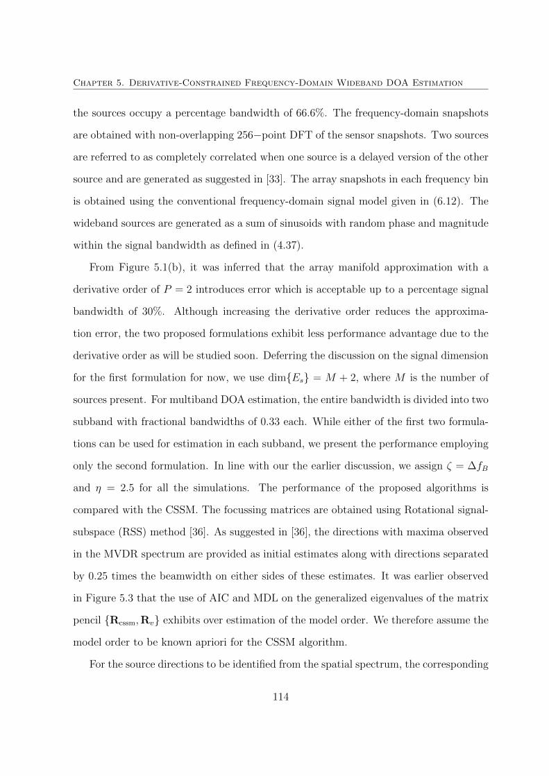
Chapter 5. Derivative-Constrained Frequency-Domain Wideband DOA Estimation
the sources occupy a percentage bandwidth of 66.6%. The frequency-domain snapshots
are obtained with non-overlapping 256−point DFT of the sensor snapshots. Two sources
are referred to as completely correlated when one source is a delayed version of the other
source and are generated as suggested in [33]. The array snapshots in each frequency bin
is obtained using the conventional frequency-domain signal model given in (6.12). The
wideband sources are generated as a sum of sinusoids with random phase and magnitude
within the signal bandwidth as defined in (4.37).
From Figure 5.1(b), it was inferred that the array manifold approximation with a
derivative order of P = 2 introduces error which is acceptable up to a percentage signal
bandwidth of 30%. Although increasing the derivative order reduces the approxima-
tion error, the two proposed formulations exhibit less performance advantage due to the
derivative order as will be studied soon. Deferring the discussion on the signal dimension
for the first formulation for now, we use dim{Es} = M + 2, where M is the number of
sources present. For multiband DOA estimation, the entire bandwidth is divided into two
subband with fractional bandwidths of 0.33 each. While either of the first two formula-
tions can be used for estimation in each subband, we present the performance employing
only the second formulation. In line with our the earlier discussion, we assign ζ = ∆fB
and η = 2.5 for all the simulations. The performance of the proposed algorithms is
compared with the CSSM. The focussing matrices are obtained using Rotational signal-
subspace (RSS) method [36]. As suggested in [36], the directions with maxima observed
in the MVDR spectrum are provided as initial estimates along with directions separated
by 0.25 times the beamwidth on either sides of these estimates. It was earlier observed
in Figure 5.3 that the use of AIC and MDL on the generalized eigenvalues of the matrix
pencil {Rcssm,Rv} exhibits over estimation of the model order. We therefore assume the
model order to be known apriori for the CSSM algorithm.
For the source directions to be identified from the spatial spectrum, the corresponding
114

Chapter 5. Derivative-Constrained Frequency-Domain Wideband DOA Estimation
0 100 200 300-50
-45
-40
-35
-30
-25
-20
-15
-10
-5
0
Scan direction, (deg)
P(
), d
B
220 240 260-50
-40
-30
-20
-10
0
Formulation 2Formulation 3
Formulation 1
Figure 5.4: Spatial spectrum obtained for the proposed formulations.
peaks have to be distinct from the spectrum floor. In order to observe this, we consider
a scenario with three wideband sources from 220◦, 250◦ and 258◦ with a percentage
bandwidth of 67%. For an SNR of 5 dB and J = 20 frequency-domain snapshots, the
spatial spectrum obtained by the three formulations are plotted in Figure. 5.4. We note
that all the three techniques provide precise DOA estimates from the spatial spectrum.
Without knowledge of the model order, the second and third formulations are observed
to provide peaks only along the source directions while the spatial spectrum in all other
directions is almost flat.
The appropriate choice of signal subspace dimension of Rav is essential for the first
formulation which realizes the BFW-MUSIC algorithm in frequency domain. To observe
the effect of this factor on the performance, we plot the spatial spectrum of Formulation
1 when sources are situated at 12◦, 40◦ and 48◦ and dim{Es} is varied from M to M + 3.
From the spatial spectra plotted in Figure 5.4.1, we observe that the technique cannot
115

Chapter 5. Derivative-Constrained Frequency-Domain Wideband DOA Estimation
0 50 100 150 200 250 300 350−45
−40
−35
−30
−25
−20
−15
−10
−5
0
Scan direction, φ (deg)
P(φ
), d
B
10 20 30 40 50
−30
−20
−10
0
dim{Es} = M
dim{Es} = M + 3
dim{Es} = M + 1dim{Es} = M + 2
Figure 5.5: Spatial spectrum for various signal subspace dimensions of Rav.
resolve the three sources when dim{Es} is equal to M or M + 1, whereas the sources
are accurately resolved for the rest of the values. When dim{Es} = M + 3, we observe
false peaks along some non-source directions due to insufficient degrees-of-freedom for the
weight vector solution. For the case where L = 10 and P = 2, if dim{Es} = M+3 = 6, the
degrees of freedom available for the weight vector solution is only 2 which is insufficient
to withhold false peaks. One potential way to estimate the signal subspace dimension
of the averaged covariance matrix Rav is to employ either AIC or MDL with a modified
penalty function. While further investigation of this approach is a part of our future
work, we employ dim{Es} = M + 2 for all our simulations which has been observed to
provide consistent results for various combinations of L,M and P .
We now consider the case when sources are completely correlated. In [33], it was
shown that the frequency averaging of coherent signal subspaces obtained from various
frequency bins can restore the rank of source correlation matrix. Likewise, the rank of
the source correlation matrix is restored with frequency averaging performed in (5.8).
116
Chapter 5. Derivative-Constrained Frequency-Domain Wideband DOA Estimation
Therefore, the proposed formulations are expected to resolve coherent sources present in
the scenario. For illustration, we consider three sources situated at 12◦, 40◦ and 48◦ and
DOA is estimated with the double-ring array. The coherent source at 48◦ is obtained
as a delayed version of the second source by 40Ts, where Ts is the sampling period.
At an SNR of 5 dB, the spatial spectrum obtained for the proposed formulations using
J = 20 snapshots is shown in Figure 5.6. We note that the three formulations are able
0 50 100 150 200 250 300 350-45
-40
-35
-30
-25
-20
-15
-10
-5
0
Scan direction, (deg)
P(
), d
B
10 20 30 40 50-40
-30
-20
-10
0
Formulation 2Formulation 1
Formulation 3
Figure 5.6: Spatial spectrum obtained for the two proposed formulations. Sources locatedat 40◦ and 48◦ are completely correlated.
to resolve all the source directions. More specifically, accurate DOA estimation using
Formulation 2 and Formulation 3 are appealing considering the fact that model order
estimation in coherent scenario is very challenging.
117
Chapter 5. Derivative-Constrained Frequency-Domain Wideband DOA Estimation
5.4.2 Performance Evaluation
Since the proposed methods incorporate capability to handle wideband sources into the
formulations of existing narrowband DOA estimation techniques, it is essential to study
the performance of the Formulations 1 and 2 with the processing bandwidth used to
evaluate Rav. For a scenario with three sources situated at 12◦, 40◦ and 48◦, the DOA is
estimated from J = 20 frequency-domain snapshots acquired by the double-ring array.
With the spectrum of all the wideband sources centered at a normalized frequency of
fc = 0.3, their fractional bandwidths is increased from 0.01 to 0.67. We first study the
probability of resolving the three sources against the fractional bandwidth of the sources
in Figure 5.10(a) for the narrowband MUSIC algorithm with model order estimated using
MDL and Formulations 1 and 2.
It is evident that the MUSIC algorithm completely fails to resolve the sources as the
processing fractional bandwidth increases to 0.1. However, the proposed formulations
can resolve the sources for larger source bandwidths with a probability of 1. When the
fractional bandwidth is increased, it is important to note that the signal subspace of Rav is
also increased. Since the first formulation employs a fixed signal subspace dimension over
the entire simulation, we note that the techniques fails to resolve the source directions
after a specific signal bandwidth. The second formulation however continues to resolve
the source directions even when the source bandwidth is increased beyond with larger
bandwidths.
In the accompanied simulation, we study the RMSE of the DOA estimates over 100
Monte-Carlo trials as a function of the processing bandwidth for the same source-sensor
setup. The RMSE of the three DOA estimates are averaged and plotted against the
fractional bandwidth in Figure 5.10(b). Since the narrowband MUSIC algorithm fails to
resolve the three sources, the corresponding RMSE plot is not shown. We note that the
118

Chapter 5. Derivative-Constrained Frequency-Domain Wideband DOA Estimation
0 0.1 0.2 0.3 0.4 0.5 0.60
0.2
0.4
0.6
0.8
1P
robabili
ty o
f R
eso
lutio
n
Fractional bandwidth
(a)
0.1 0.2 0.3 0.4 0.5 0.60
0.5
1
1.5
Fractional bandwidth
RM
SE
(deg)
(b)
Formulation 1
Formulation 2
Formulation 1
NarrowbandMUSIC
Formulation 2
Figure 5.7: DOA estimation performance against fractional bandwidth being processed:(a) probability of resolving the closely-situated sources, (b) RMSE of estimates averagedover the three sources.
RMSE from Formulations 1 and 2 starts to increase with the fractional bandwidth when
∆f is approximately greater than 0.25.
We now evaluate the performance of the DOA estimates obtained from the three
formulations in comparison with existing techniques. We limit our comparison only to
the TD-DOA technique proposed in the previous chapter and CSSM since the TOPS
algorithm and ISSM are known to have limited performance at low SNR conditions
as shown in Section 4.5. With J = 10 frequency domain snapshots and a fractional
bandwidth of ∆f = 0.25, the RMSE of DOA estimates evaluated over 100 independent
trials is plotted against SNR in Figure 5.8.
119

Chapter 5. Derivative-Constrained Frequency-Domain Wideband DOA Estimation
We note that the RMSE of the estimates decrease with increasing SNR for all the
techniques except for TD-DOA proposed in Chapter 4. The approximation of array
manifold over such a large bandwidth with Taylor series of order 2 introduces a large
error in the estimated DOA. Therefore, the estimation performance does not improve
significantly when the SNR is increased. The CSSM exhibits the best performance for
the first and third sources, while the RMSE is relatively large for the second source
till an SNR of 10 dB. This is because of its dependence on the initial estimates. The
inability to resolve the three sources by MVDR [36] provides inaccurate initial estimates
for the focussing matrix design, resulting in an estimation error. As the SNR increases
beyond 10 dB, the MVDR algorithm succeeds in providing the three initial directions
estimates, which improves the DOA estimation. This observation reflects the sensitivity
of CSSM to initial estimates. Among the three proposed formulations, we observe that
Formulation 1 performs better than the other two formulations at low SNR values. As
the SNR is increased, the performance of Formulation 2 approaches that of Formulation 1
even without the knowledge of model order. This observation can be accounted for the
improved segregation between signal and noise subspaces at high SNR values and the
automated choice of β. As expected, the processing of multiple subbands yields improved
results over the entire SNR range over Formulation 2 which uses only one subband.
Figure 5.9 shows the probability of resolving all the three sources against SNR for the
previous simulation. Among the proposed formulations, the first formulation has better
resolution over the other two formulations. It is interesting to note that the second
formulation has the same resolution capability as that of the TD-DOA technique. This
is due to the MUSIC-like framework being employed for DOA estimation in contrast to
the subspace-based approach which provides better resolution for Formulation 1. The
corresponding multiband scheme is observed to yield marginal improvement in resolving
the sources. Although CSSM exhibits better resolution over the proposed techniques,
120
Chapter 5. Derivative-Constrained Frequency-Domain Wideband DOA Estimation
this performance is susceptible to the initial estimates and the model order.
In Figure 5.8, it was noted that the RMSE for Formulations 1 and 2 almost saturate
when the SNR is increased beyond 10 dB for the last two sources. This phenomenon
surfaces when the SNR is high, for which case the effect of sensor noise is lesser than the
residual error introduced due to the incomplete suppression of all the derivative terms
in Rav by the derivative constraints. In order to study this phenomenon, the derivative
order was fixed to P = 2 and we study the performance of Formulation 2 with SNR for
various processing bandwidths of the sources. The array geometry and source directions
are maintained the same as the previous simulation and the RMSE of the second source
direction estimate obtained by Formulation 2 is observed in Figure 5.10. We note that the
RMSE for various processing bandwidths of the sources decreases as the SNR increases
upto a specific SNR and saturates without decreasing further. This saturation point can
be identified as the situation when the additive noise variance is lower than the residual
error due to incomplete suppression of the derivative terms. Furthermore, the SNR
at which the RMSE curve saturates is observed to decrease with increasing processing
bandwidth. For a fixed order of derivative compensation, this observation indicates that
the residual error increases with the processing bandwidth.
We next study the effect of the number of frequency-domain snapshots on the DOA
estimates for the same simulation setup at 5 dB SNR in Figure 5.11. Among the three
sources, we note that the estimate for the first source shows lower RMSE due to the large
spatial separation from other sources. The first formulation is observed to have the least
RMSE when compared to all other techniques. CSSM is seen to be less sensitive to the
variations in the number of snapshots, while the RMSE of the proposed Formulation 2
decreases as the number of snapshots increases. The multiband DOA estimation devel-
oped over Formulation 2 is observed to have better performance over it, indicating the
need to exploit DOA estimation across the entire bandwidth.
121
Chapter 5. Derivative-Constrained Frequency-Domain Wideband DOA Estimation
5.5 Discussions and Concluding Remarks
In this chapter, we first observed that the AIC and MDL techniques over-estimate the
number of sources present in the scenario when used with the coherently averaged covari-
ance matrix Rcssm. This result would adversely affect the performance of CSSM if the
model order is obtained incorrectly. From the simulations studies, it is observed that all
the three formulations can estimate wideband source directions. The first formulation,
built over the BFW-MUSIC, requires to estimate the signal subspace dimension which
is generally greater than the model order. With the signal subspace dimension approx-
imately known, this formulation can suppress the derivative components present in the
covariance matrix effectively, thus yielding better estimation accuracy over the other two
formulations. However, the problem of model order estimation is still unresolved with
the outcome of this formulation.
In order to estimate wideband source directions independent of the model order es-
timation problem, we present the second formulation employing the MUSIC-like formu-
lation. This is a frequency domain realization of the proposed algorithm in Chapter 4.
This algorithm maintains the accuracy of estimates even for sources with large bandwidth
by regulating the processing bandwidth. The third formulation extends the second for-
mulation over multiple subbands in order to exploit the DOA information preserved in
other source subbands. We therefore achieve a means to estimate directions of wideband
sources whose percentage bandwidth can be from 10− 67%.
122
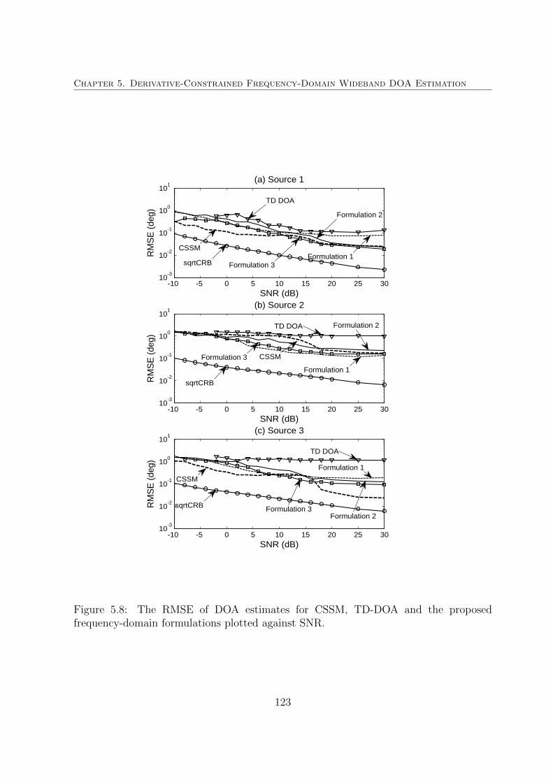
Chapter 5. Derivative-Constrained Frequency-Domain Wideband DOA Estimation
-10 -5 0 5 10 15 20 25 3010
-3
10-2
10-1
100
101
RM
SE
(de
g)
SNR (dB)
(a) Source 1
-10 -5 0 5 10 15 20 25 3010
-3
10-2
10-1
100
101
RM
SE
(de
g)
SNR (dB)
(b) Source 2
-10 -5 0 5 10 15 20 25 3010
-3
10-2
10-1
100
101
RM
SE
(de
g)
SNR (dB)
(c) Source 3
TD DOA
Formulation 3sqrtCRB
CSSM
Formulation 2
Formulation 1
sqrtCRB
CSSMFormulation 3
TD DOA Formulation 2
Formulation 1
sqrtCRB
CSSM
TD DOA
Formulation 3Formulation 1
Formulation 2
Figure 5.8: The RMSE of DOA estimates for CSSM, TD-DOA and the proposedfrequency-domain formulations plotted against SNR.
123

Chapter 5. Derivative-Constrained Frequency-Domain Wideband DOA Estimation
-20 -10 0 10 20 300
0.1
0.2
0.3
0.4
0.5
0.6
0.7
0.8
0.9
1
Pro
babi
lity
of R
esol
utio
n
SNR (dB)
Formulation 3CSSM
Formulation 1
TD-DOA
Formulation 2
Figure 5.9: The probability of resolving all the three sources plotted against SNR forvarious formulations.
0 5 10 15 2010
-2
10-1
100
RM
SE
(de
g)
SNR (dB)
fB = 0.25
fB = 0.34
fB = 0.4
fB = 0.5
Figure 5.10: The plot of RMSE for the second source direction estimate using Formulation2 for various processing bandwidths.
124

Chapter 5. Derivative-Constrained Frequency-Domain Wideband DOA Estimation
5 10 15 20 25 30
10-2
10-1
100
RM
SE
(deg)
No. of frequency domain snapshots
(a) Source 1
5 10 15 20 25 30
10-2
100
RM
SE
(deg)
No. of frequency domain snapshots
(b) Source 2
5 10 15 20 25 30
10-2
100
RM
SE
(deg)
No. of frequency domain snapshots
(c) Source 3
CSSM
sqrtCRB
Formulation 3
TD DOA
TD DOA
CSSM
Formulation 3Formulation 2
Formulation 2Formulation 3
Formulation 1
Formulation 1CSSM sqrtCRB
Formulation 1
TD DOA
sqrtCRB
Formulation 2
Figure 5.11: The RMSE of DOA estimates plotted against the number of frequency-domain snapshots used.
125

Chapter 6
Wideband DOA Estimation in
Dispersive Medium
6.1 Introduction
The DOA estimation techniques discussed in previous have been developed considering
homogeneous nondispersive medium. In practical scenarios however, environmental fac-
tors such as multipath, scattering and dispersion [50] may have to be incorporated into
the signal model. Conventional techniques therefore cannot be directly employed to local-
ize sources in such conditions. Among these factors, dispersion is a common phenomenon
due to which different frequency components within a wave propagate at different speeds.
In a homogeneous medium, dispersion is observed when the relative permittivity and/or
permeability of the medium are/is a function of frequency. Whereas in a heterogeneous
medium, effects such as scattering due to suspended particles affect the speed of propa-
gation. Often, dispersion is studied with the “dispersion curve” obtained by plotting the
wavenumber or speed against angular frequency.
For wireless applications, the access bandwidth within the conventional frequency
126

Chapter 6. Wideband DOA Estimation in Dispersive Medium
spectrum is very limited; the spectrum with wavelength in millimeter range corresponding
to frequencies beyond 30 GHz is available for usage. At these frequencies, however, the
atmospheric transfer function exhibits significant frequency-dependent attenuation and
phase delay as pointed out in [51]. The absorption, dispersion and scattering of signals
due to atmospheric elements as well as the rain drops, can be cumulatively incorporated
within the atmospheric transfer function [50]. For ultra-wideband pulse propagation,
the expressions for time-delay and the pulse width variations are shown in [50] to be
functions of first and second-order derivatives of attenuation and phase delay factors
w.r.t. frequency. This dependence over frequency translates to dispersive effect. Besides
these factors which exist in clear sky conditions, variations in time-delay due to rain are
susceptible to parameters such as rain drop size and rain-rate. It is therefore challenging
to precisely estimate and compensate for dispersive effect prior to DOA estimation. A
robust estimator is hence essential to obtain reliable estimates in such situations.
In other applications such as seismic and underwater acoustics, the medium is het-
erogeneous in nature due to the presence of suspended particles. As a consequence,
the wave encounters absorption, refraction, reflection and dispersion while propagating
through the medium. Furthermore, the wave propagation speed is a continuous func-
tion of depth in these applications and has to be compensated based on location specific
sound speed profiles. Under such conditions, signal parameters are estimated by modeling
these uncertainties as either multiplicative noise [52] or as wavefront amplitude distor-
tion [53]. An alternative approach is to employ matched-field processing [54] framework
to estimate the source location by evaluating the received power from each possible lo-
cation. This framework permits the incorporation of wave solution and robustness to
random speed perturbations into the constraint equations of MVDR algorithm as shown
in [55]. The maximum likelihood estimator in [55] is however developed for the narrow-
band signal model. This principle can easily be extended to wideband sources with the
127

Chapter 6. Wideband DOA Estimation in Dispersive Medium
STCM-MVDR algorithm [40] reviewed in Section 2.3.2.4. Across the signal bandwidth,
the steered covariance matrix in a given azimuth φ is constructed as
R(φ) =
fu∑fk=fl
TH(fk, φ)R(fk)T(fk, φ), (6.1)
where T(fk, φ) = diag{a(fk, φ)}. If we define a diagonal matrix U(fk) which incorporates
a frequency-dependent speed perturbation, the STCM can be modified as
R1(φ) =
fu∑fk=fl
U(fk)TH(fk, φ)R(fk)T(fk, φ)UH(fk). (6.2)
The source directions can then be estimated from the peaks of the steered response as
P (φ) =1
1TLR−11 (φ)1L
. (6.3)
We use this technique as the baseline algorithm in our study.
Our objective in this chapter is to estimate wideband source directions in a dispersive
medium. Due to inaccurate knowledge of the dispersion curve, we assume that the prop-
agation speed is an unknown continuous function of frequency. With this assumption,
we can express the steering vector at a reference frequency as a Taylor series expansion
w.r.t. the wavenumber within the signal bandwidth. An averaged covariance matrix
can then be estimated across the signal bandwidth which consists of derivative terms
w.r.t. wavenumber. We then employ the structure of MUSIC-like algorithm for DOA
estimation by introducing robustness to dispersion. With an average propagation speed
known only at the reference frequency, the proposed technique estimates DOA without
requiring the dispersion curve. The chapter is structured as follows: In Section 6.2, we
first derive the signal model for homogeneous dispersive medium. The array manifold
128
Chapter 6. Wideband DOA Estimation in Dispersive Medium
approximation is incorporated into the signal model in Section 6.3. We then propose
a DOA estimation technique in Section 6.4 which introduces robustness to variations
in speed over frequency. The performance of the proposed technique is evaluated with
simulations in Section 6.5 and Section 6.6 concludes this chapter.
6.2 Signal Model
A wideband signal, if represented as a sum of sinusoids, can be written as a composite
modulated signal. For instance, a signal with two sinusoids at angular frequencies ω1 =
2πf1 and ω2 = 2πf2 is given by
s(t) = sin(ω1t) + sin(ω2t)
= 2 sin(ωt) cos(δωt),
(6.4)
where ω = (ω1 +ω2)/2 and δω = (ω1−ω2)/2. In a homogeneous medium, this travelling
wave at a spatial point r can be expressed as
s(t−α.r) = 2 cos(δωt− δκ.r) sin(ωt− κ.r), (6.5)
where α is the slowness vector and δκ = δωα is the differential wavenumber vector for the
two frequencies. We note that the signal consists of a carrier signal component sin(ωt−
κ.r) and a modulating signal component cos(δωt− δκ.r). The velocities estimated from
the respective components are termed as the phase and group velocities. Phase velocity
is the rate at which the carrier phase propagates in the wave propagation direction. In
its scalar form, we have
νp =ω
κ, (6.6)
129

Chapter 6. Wideband DOA Estimation in Dispersive Medium
where κ = |κ| is the magnitude of the wavenumber vector. The group velocity is the
propagation speed of the modulating signal or the envelop. In its scalar form
νg =δω
δκ=ω2 − ω1
κ2 − κ1
, (6.7)
where κ1 and κ2 are the wavenumbers at frequencies ω1 and ω2, respectively. For a
nondispersive medium, the phase velocity is a constant over frequency. From (6.6), we
hence have
ω1 = νpκ1,
ω2 = νpκ2.
(6.8)
Substituting (6.8) into (6.7), it is easy to note that the group velocity is equal to the phase
velocity. However, since the permittivity and/or permeability of a dispersive medium
varies with frequency, this equality is not maintained. It is also possible to show that these
velocities, and the corresponding slowness vectors (α) are related by simple geometric
relations [56].
The slowness vector is related to the phase velocity as
α =|α|u =1
νpu. (6.9)
where u denotes a unit vector in the direction of wave propagation. Since the propagation
speed varies with frequency for a dispersive medium, we note that the slowness vector is
a function of frequency, i.e., α(f). When a propagating signal is acquired by an array of
L sensors at spatial locations r1, r2, ..., rL, the sensor outputs in frequency domain can
130

Chapter 6. Wideband DOA Estimation in Dispersive Medium
be obtained using the Fourier transform relation in (2.30) as
x(f) =
e−2πfα(f).r1
e−2πfα(f).r2
...
e−2πfα(f).rL
s(f) + v(f)
= a(f, ν(f), θ)s(f) + v(f),
(6.10)
where ν(f) = 1/|α(f)| is the frequency-dependent propagation speed. Note that this
model holds true even when the source signal has more than two sinusoids. The source
model can be expressed as
s(t) =
Bbw∑i=1
aiexp{(2πfit+ ci)}, (6.11)
where the amplitude ai is an instance of Rayleigh distribution, ci is uniformly distributed
in [−π, π] and Bbw is the number of sinusoids that constitute the wideband source. Since
the phase velocity and group velocity are related by geometric relations in a dispersive
medium [56], an explicit presence of group velocity in the signal model need not be
considered. Extending the signal model in (6.10) for a scenario with M sources from
directions Θ = [θ1, ..., θM ], we have
x(f) = A(f, ν(f),Θ)s(f) + v(f), (6.12)
with A(f, ν(f),Θ) = [a(f, ν(f), θ1), . . . , a(f, ν(f), θM)] is the array manifold matrix. The
problem in hand is to estimate the source directions Θ from the sensor snapshots.
131

Chapter 6. Wideband DOA Estimation in Dispersive Medium
6.3 Array Manifold Approximation
Since the slowness vector and the wavenumber vector are related by
κf = ωα(f) =2πf
ν(f)u = κfu, (6.13)
the wavenumber κf = 2πf/ν(f) absorbs the dispersion factor which affects the steering
vector. We can therefore rewrite the steering vector as a function of wavenumber instead
of frequency as
a(κf , φ) =[e−κfu.r1 e−κfu.r2 . . . e−κfu.rL
]T. (6.14)
If we define a reference frequency f0 at which the propagation speed is estimated ν(f0),
the wavenumber at a frequency bin in the proximity of f0 can be approximated with
Taylor series of order P w.r.t. κf as
a(κf , φ) ≈ a(κ0, φ) +P∑p=1
(δκf )p
p!
∂a(κf , φ)
∂kf
∣∣∣κf=κ0
, (6.15)
where κ0 = 2πf0/ν(f0) is the wavenumber at frequency f0 and δκf = κf−κ0. We can ex-
press the array manifold matrix A(κf ,Θ) in terms of κ0 with Taylor series approximation
using which, the signal model at frequency fk is given by
x(k, l) ≈(A(κ0,Θ) +
P∑p=1
(δκf )p
p!
∂pA(κf ,Θ)
∂κpf
∣∣∣κf=κ0
)s(k, l) + v(k, l). (6.16)
132

Chapter 6. Wideband DOA Estimation in Dispersive Medium
With this approximation, the spatial covariance matrix for the zero-mean snapshots
x(k, l) at fk is given by
R(fk) ≈A(κ0,Θ)Rss(fk)AH(κ0,Θ) + σ2
v(fk)IL
+L∑p=1
(δκf )p
p!Re[A(κ0,Θ)Rss(fk)
∂p
∂κpfAH(κf ,Θ)
∣∣∣κf=κ0
]+
P∑p,q=1
δκp+qf
p!q!
∂p
∂κpfA(κf ,Θ)
∣∣∣κf=κ0
Rss(fk)∂q
∂κqfAH(κf ,Θ)
∣∣∣κf=κ0
,
(6.17)
where σ2v(fk) is the variance of the additive uncorrelated sensor noise at frequency fk. We
note that the derivatives of A(κf ,Θ) w.r.t. the wavenumber distinguishes (6.17) from
the expression for R(fk) in (5.3). Therefore, following the previous approach adopted
for frequency-domain wideband DOA estimation, we first define a fractional bandwidth
∆fB < ∆f corresponding to B + 1 frequency bins in the proximity of f0, over which a
P th order Taylor series approximates the array manifold up to an acceptable error. An
average covariance matrix across this bandwidth can then be defined as
Rav =1
B + 1
B/2∑k=−B/2
R(fk)
≈ 1
B + 1
[A(κ0,Θ)
{ k0+B/2∑k=k0−B/2
Rss(fk)
}AH(κ0,Θ)
+ 2
k0+B/2∑k=k0−B/2
Re
{ P∑p=1
(δκf )p
p!A(κ0,Θ)Rss(fk)
∂p
∂κpfAH(κf ,Θ)
∣∣∣∣κf=κ0
}
+
k0+B/2∑k=k0−B/2
P∑p,q=1
(δκf )p+q
p!q!
∂p
∂f pA(κf ,Θ)
∣∣∣∣κf=κ0
Rss(fk)AH(κf ,Θ)
∣∣∣∣κf=κ0
+
k0+B/2∑k=k0−B/2
σ2v(fk)IL
].
(6.18)
This matrix consists of the familiar coherently averaged component and the derivative
terms observed in (5.8). Suppressing the derivative terms will therefore reduce the prob-
133

Chapter 6. Wideband DOA Estimation in Dispersive Medium
lem to narrowband DOA estimation.
6.4 Proposed Technique
When the model order is not available, employing the framework of narrowband MUSIC-
like algorithm provides better resolution over the MVDR algorithm. We first define a
matrix Dκ0,φ with derivative vectors up to P th order from each look direction φ as
Dκ0,φ =[d1(κ0, φ) d2(κ0, φ) . . . dP (κ0, φ)
], (6.19)
where dp(κ0, φ) =∂pa(κf ,φ)
∂κpf
∣∣∣κf=κ0
. The projection matrix of Dκ0,φ is given by
PDφ= Dκ0,φ(DH
κ0,φDκ0,φ)−1DH
κ0,φ.
The data matrices at each frequency X(k), are concatenated over the processing band-
width (B + 1 bins) to obtain
X =[X(−B/2), . . . ,X(B/2)
]∈ CL×J(B+1). (6.20)
This matrix is projected onto the derivative vector space in each look direction as Y =
PDφX. The corresponding covariance matrix is given by
Ry(φ) = PDφRavP
HDφ. (6.21)
134
Chapter 6. Wideband DOA Estimation in Dispersive Medium
Introducing this term into the optimization problem, we have
minimizewφ
wHφ
{Rav + ζRy(φ)
}wφ
subject to wHφ
{a(κ0, φ)aH(κ0, φ) + βIL
}wφ = c,
(6.22)
where β, ζ, c are constants. The optimal weight vector is given by the eigenvector corre-
sponding to the minimum eigenvalue χmin of the GEV,
(Rav + ζRy(φ)
)wφ = χmin
(a(κ0, φ)aH(κ0, φ) + βIL
)wφ. (6.23)
With the processing bandwidth limited to B + 1 frequency bins, the parameter ζ can be
assigned a value equal to the fractional bandwidth ∆fB = B+1f0
based on the discussion
presented in Section 4.3.2. Likewise, the bounds derived for β in the TD-DOA algorithm
can be extended to this context by replacing the time-domain covariance matrix R with
Rav. The value of β is chosen with reference to the lower bound as
β = η minφ
aH(κ0, φ)(R + ζRy(φ)
)−1a(κ0, φ)
χ(R+ζRy(φ))−1,max
, (6.24)
where η > 1 provides unambiguous spatial spectrum when it is chosen such that β is
within the bounds. We observe that the proposed technique for DOA estimation under
dispersive medium is an extension of the technique discussed in Chapter 5 and only
differs in using the derivative terms w.r.t. the wavenumber instead of frequency. Since
the dispersion was preserved in the derivative terms of (6.18), their suppression using the
proposed formulation enhances its robustness to dispersion.
135

Chapter 6. Wideband DOA Estimation in Dispersive Medium
6.5 Simulation Results and Discussions
In this section, we evaluate the performance of the proposed technique under a simulated
dispersive environment. In this section all the frequencies are normalized such that the
sampling frequency is equal to unity. The propagation speed is synthesized from a simple
nonlinear function of frequency f given by
ν(f) = ν(fc)(
1 + ∆νmax tanh(γ(f − fc))), (6.25)
where ∆νmax = ν(fmax)−ν(fmin)ν(fc)
is the fractional speed variation across the signal bandwidth
which is centered at the normalized frequency fc with speed ν(fc) and γ > 0 regulates
the nonlinearity of the function. When γ = 0, the propagation speed remains constant
across the signal bandwidth. Noting that the dispersion relation for freely propagating
ocean surface gravity waves obeys a hyperbolic tangent function [57], we have introduced
∆νmax and γ > 0 in order to regulate the degree of nonlinearity in (6.25). Moreover,
the theoretical Love and Rayleigh dispersion curves for a seismic two-layer model [58]
can be synthesized with (6.25). The dispersion observed in atmosphere can similarly be
modeled using the same function. The frequency-domain signal model given by (6.12) is
used for the simulations in this section and the source signals are generated using (6.11).
The frequency dependent array manifold matrix A(f, ν(f),Θ) is obtained using the wave
velocity function given by (6.25).
The proposed technique is compared with the STCM-MVDR algorithm, which fol-
lows a matched-field processing structure. If the dispersion curve is available, it can be
incorporated in the steered vectors used while estimating the steered covariance matrix.
For the proposed technique, we provide only the propagation speed ν(fc) at fc, while
for the STCM-MVDR we provide the dispersion curve given by (6.25). A derivative
order of P = 2 is used to construct Dκ0,φ. The propagation speed at frequency fc = 0.3
136

Chapter 6. Wideband DOA Estimation in Dispersive Medium
considering wireless applications is chosen to be ν(fc) = 3 × 10⁸ m/s. We use J = 20
frequency-domain snapshots for all the simulations.
We first study the spatial spectrum of the proposed technique for a scenario with a
4×4 planar array with an inter-element spacing of d = λmin/2 is used for this simulation.
Two wideband sources with a fractional bandwidth of ∆f = 0.33 and centered at fc = 0.3
are situated at azimuth angles 40◦ and 60◦ in the same plane as the array. The elevation
angle is therefore equal to zero. The propagation speed varies according to the dispersion
function given by (6.25) with ν(fc) = 3×10⁸ m/s and a percentage speed deviation of 5%
(∆νmax = 0.05). Two instances with of dispersion curve with γ = −60 and γ = 60 shown
in Fig. 6.1(a) are used for the simulation. While the dispersion curve for γ = −60 is a
monotonically decreasing function, the speed increases with frequency for γ = 60. The
frequency-domain snapshots are obtained by introducing dispersion according to (6.12)
at an SNR of 5 dB. The spatial spectra obtained by the proposed technique for the
two dispersion functions with 20 frequency-domain snapshots are plotted in Fig. 6.1(b).
We note that the spatial spectrum for the proposed technique exhibits distinct peaks
along the two source directions. With only the center frequency provided, the algorithm
is observed to be robust for changes in speed over a percentage speed deviation of 5%
within the source bandwidth.
It is important to note that the proposed technique provides accurate estimates with-
out the use of dispersion curve. This indicates that the proposed technique exhibits
robustness for various degrees of dispersion nonlinearity. In order to verify this, we in-
vestigate the performance of the proposed technique with the RMSE of DOA estimates
over various degrees of nonlinearity obtained by regulating the parameters γ and ∆νf in
(6.25). For the simulation setup used before, we plot the RMSE of the estimates averaged
over the two sources against ∆νf and γ in Fig. 6.2(a) and (b), respectively. We plot the
performance of the STCM-MVDR algorithm under the same simulation setup. We note
137

Chapter 6. Wideband DOA Estimation in Dispersive Medium
0.2 0.25 0.3 0.35 0.42.9
2.92
2.94
2.96
2.98
3
3.02
3.04
3.06
3.08
3.1x 10
8
Normalized frequency, f/fs
Pro
pagation
spee
d,ν(f
)
(a)
0 20 40 60 80 100 1200
5
10
15
20
25
30
35
40
45
50
Scan direction, φ (deg)
Pow
er(d
B)
(b)
γ= 60γ= −60
γ= −60 γ= 60
Figure 6.1: (a) Dispersion function with the propagation speed plotted against frequencyfor γ = −60 and γ = 60. (b) Spatial spectrum obtained by the proposed technique forthe two values of γ with SNR set to 5 dB.
that the proposed technique has improved estimation accuracy over the STCM-MVDR
algorithm for all values of ∆νf and γ. From Figure 6.2(a) and (b), it is important to
note that the estimation accuracy is almost constant over the entire range of ∆νf and
γ, which implies that the proposed technique is robust to different nonlinear functions.
This is due to the incorporation of Ry(φ) which provides robustness to any monotonic
change in speed from νc at the center frequency.
We next study the variation in performance of the proposed technique with SNR
in comparison with the STCM-MVDR algorithm for the same simulation setup. The
simulation is conducted for γ = −50 and γ = 50 maintaining a ∆νf = 0.05. The
RMSE of individual source estimates are plotted in Figure 6.3. The proposed technique
is observed to provide improved estimation accuracy over the STCM-MVDR algorithm
at lower SNR values. For both the values of γ, we note that the accuracy is very similar
as expected.
In all the above simulations, the dispersion function employed is idealistic with speed
138

Chapter 6. Wideband DOA Estimation in Dispersive Medium
0.02 0.04 0.060
0.2
0.4
0.6
0.8
1
RM
SE
(deg)
max
(b)
-60 -40 -20 0 20 40 600.3
0.4
0.5
0.6
0.7
0.8
0.9
1
RM
SE
(deg)
Nonlinearity,
(a)
Proposed TechniqueSTCM-MVDR
Proposed TechniqueSTCM-MVDR
Figure 6.2: Estimation performance of the proposed technique plotted against the non-linearity function parameters, (a) γ, (b) ∆νmax.
monotonically increasing or decreasing as frequency increases. We now consider a prac-
tical situation with propagation speed perturbed with random fluctuations across the
signal bandwidth as shown in Figure 6.4(a). This scenario is encountered in seismic
applications where phase velocity is sensitive over different layers of the soil [58]. For
the same source directions and array geometry used for the previous simulation, the
dispersion function shown in Figure 6.4(a) is obtained as
νf = νc
(1 + ∆νmax tanh(γ(f − fc))
)+ δνc, (6.26)
where δνc is a random speed fluctuation derived from Gaussian distribution.
Allowing the speed at the center frequency to be ν(fc) = 1000 m/s, a percentage speed
dispersion of 10% (∆νmax = 0.1) is introduced for this simulation. With only the speed at
center frequency known, the spatial spectrum of the proposed technique obtained at an
SNR of 0 dB is plotted in Figure 6.4(b) in comparison with the performance of the STCM-
139

Chapter 6. Wideband DOA Estimation in Dispersive Medium
-5 0 5 10 15 20 250
1
2
3
4
RM
SE
(deg)
SNR (dB)
(a) Source 1
-5 0 5 10 15 20 250
1
2
3
4
RM
SE
(deg)
SNR (dB)
(b) Source 2
Proposed TechniqueSTCM-MVDR
Proposed TechniqueSTCM-MVDR
= 60
=-60
= 60
=-60
Figure 6.3: (a) Estimation performance of the proposed technique plotted against SNRfor, (a) Source 1, (b) Source 2.
MVDR algorithm. We note that the spatial spectrum of the proposed technique shows
accurate peaks along the source directions in contrast to STCM-MVDR which has poorer
resolution. This robustness to speed perturbations can be explained by first realizing that
narrowband MUSIC-like formulation introduces deep nulls along the source directions.
The introduced derivative compensation widens the null width along the wavenumber
axis depending on the derivative order included.
140

Chapter 6. Wideband DOA Estimation in Dispersive Medium
0.2 0.25 0.3 0.35 0.4850
900
950
1000
1050
1100
1150
Normalized frequency, f/fs
Pro
pagation
spee
d,ν(f
)
(a)
0 20 40 60 80 100 1200
5
10
15
20
25
30
35
40
45
50
Scan direction, φ (deg)
Pow
er(d
B)
(b)
Proposed Technique
STCM−MVDR
Figure 6.4: (a) Dispersion function with the propagation speed obtained using(6.26)plotted against frequency. (b) Spatial spectrum obtained by the proposed tech-nique and the STCM-MVDR algorithm at an SNR of 0 dB.
6.6 Conclusion
In this chapter, we first observed that the incorporation of dispersion into the wideband
signal model affects only the array manifold matrix. The array manifold approximation
which has been adopted in previous chapters can therefore be extended to dispersive
environment with steering vectors approximated with Taylor series expansion w.r.t. the
wavenumber instead of frequency. The effect of dispersion on wideband DOA estima-
tion was then countered by incorporating a data-dependent correlation matrix into the
MUSIC-like formulation. With the propagation speed known only at a reference fre-
quency, the algorithm was observed to resolve source directions accurately. The proposed
technique has been observed to be robust to different degrees of nonlinearity verified with
synthesized dispersive curve.
141

Chapter 7
Conclusion and Future Directions
7.1 Conclusion
The central theme of this thesis has been the DOA estimation of narrowband and wide-
band sources. Having known the need to estimate the number of sources from the review
of existing techniques, the working principle of the narrowband MUSIC-like algorithm [9],
which does not require the model order information, has been investigated. The perfor-
mance of this technique is observed to approach that of MUSIC algorithm when the SNR
is increased. More interestingly, the weight vector solution obtained in each scan direc-
tion has been identified to reside in the noise subspace. This observation is exploited to
construct a weight vector matrix, the columns of which spans the noise subspace of the
array covariance matrix. With this matrix, the MUSIC-W algorithm has been presented
in Chapter 3 by replacing the noise eigenvector matrix in the MUSIC spectrum with the
weight vector matrix. From our investigations, it has been inferred that the MUSIC-
W algorithm out-performs the MUSIC-like algorithm and approaches the performance
of the MUSIC algorithm. The computational advantage and performance improvement
makes this algorithm appealing over MUSIC-like algorithm when the number of sources
142

Chapter 7. Conclusion and Future Directions
is unknown.
With the performance of MUSIC-like and MUSIC-W algorithms comparable with
the MUSIC algorithm for narrowband sources, wideband DOA estimation has been
considered with unknown number of sources in Chapter 4. Noting that the steering
vector is a function of frequency, an array manifold approximation has been exercised
using Taylor series expansion w.r.t. frequency. The expression for time-domain array
covariance matrix is then shown to have additional derivative terms along with a co-
herently averaged narrowband component. Introducing derivative compensation to the
beamforming-framework of MUSIC-like algorithm, the technique has been extended for
wideband source scenario. From the presented analysis however, it is inferred that this
compensation cannot be incorporated into the MUSIC-W algorithm. Nevertheless, the
proposed TD-DOA technique with modified MUSIC-like formulation has been observed
to provide accurate source directions by incorporating robustness against frequency vari-
ations. Unlike the BFW-MUSIC algorithm which imposes linear derivative constraints,
this technique is less sensitive to the choice of derivative order. The performance of this
technique has been shown to be comparable with CSSM and outperforms BFW-MUSIC
algorithm and TOPS algorithms when the number of snapshots is large. With model
order assumed to be unknown, the probability of resolution is marginally decreased for
this technique.
When the source bandwidth is large, the performance of TD-DOA technique has been
observed to decrease in Figure 5.2 due to the array manifold approximation error. In
order to address this problem, the BFW-MUSIC and MUSIC-like wideband DOA esti-
mation techniques have been realized in the frequency domain by constructing an average
covariance matrix over a regulated source bandwidth. Investigations reveal that the pro-
posed techniques have estimation performance comparable with CSSM and other existing
techniques. With the number of sources unknown, the frequency-domain MUSIC-like
143

Chapter 7. Conclusion and Future Directions
formulation has been observed to provide reliable estimates with marginally lower prob-
ability of resolution. The multi-band extension of this technique to extract the DOA
information from the entire signal bandwidth has been shown to improve the estimation
performance. Furthermore, the capability of these techniques to resolve closely-situated
coherent sources with unknown number of sources has been examined, in which case,
other techniques fail when incorrect number of sources is estimated.
When the medium is dispersive in nature, DOA estimation accuracy is adversely af-
fected by the speed variations. In Chapter 6, the array manifold approximation has been
redefined such that the formulation incorporates robustness to dispersion. With deriva-
tive compensation incorporated w.r.t. the wavenumber in the MUSIC-like formulation,
source directions are estimated in dispersive medium with high accuracy. The robustness
of the proposed technique to variations in propagation speed has been shown in our in-
vestigations. It is important to emphasize that this technique estimates source directions
with the propagation speed known only at the reference frequency.
Besides the topics discussed in the thesis, we also pursued with the study of DOA
estimation of speech sources under aliasing conditions. For speech sources which are
bandlimited from 400 Hz to 4 kHz, the output of a microphone array has to be sampled
abiding the spatial Nyquist criterion which requires the sensor spacing d ≤ 0.5λmin =
0.04 m, where λmin is the wavelength corresponding to the maximum signal frequency.
With number of microphones often constrained by the system design, the aperture length,
and hence the resolution of DOA estimation is limited by this condition. While the
extension of microphone spacing beyond Nyquist criterion improves the resolution, it is
complemented with the introduction of spatial aliasing.
As shown in [59], the effect of aliasing on wideband DOA estimation exhibits itself
with raised spatial spectrum floor unlike in the narrowband scenario which provides
distinct aliasing peaks. This phenomenon adversely affects the identifiability of source
144

Chapter 7. Conclusion and Future Directions
directions from the spatial spectrum in a reverberant scenario, more so when the number
of sources is not known accurately. Therefore, it is required to suppress the spectrum
floor while maintaining the source direction peaks following a detailed analysis of aliasing
effect on wideband speech sources.
In order to imporve the identifiability of source directions, we have proposed a multi-
stage scheme in [J5] based on a careful analysis, where we note that the effect of aliasing
on microphone outputs varies over different bands within the source bandwidth. Based
on this observation, we first decompose the microphone signals into different subbands
depending on the degree of aliasing that affects each subband. The alias-free spatial
spectrum obtained by performing DOA estimation on the first subband is employed in
the second stage to inhibit any DOA ambiguity introduced due to aliasing in the spa-
tial spectrum of the second subband. The resultant spectrum is then employed in the
succeeding stages to suppress the effect of aliasing while maintaining the high resolution
speech DOA estimation obtained by the latter stage. This multi-stage scheme has been
verified with a beamforming-based technique (STCM-MVDR) and a time-difference of
arrival-based technique (approximate kernel density estimator (KDE) [60],2012Nesta).
It is observed that the proposed scheme enhances the identifiability of the source direc-
tions in the spatial spectrum while maintaining the accuracy of the baseline algorithm
employed. This discussion was not included as a part of the thesis due to its mismatch
with the rest of the chapters in the thesis.
7.2 Future Directions
In the due course of this research, a few potential extensions were identified. Since the
involving work steps beyond the outline of this thesis, we enlist them here inviting interest
from researchers.
145

Chapter 7. Conclusion and Future Directions
• One of our interesting findings is the MUSIC-W algorithm developed for narrow-
band DOA estimation. Constructing the weight vector matrix from arbitrary di-
rections was observed to substitute the need to estimate the noise subspace, as well
as the model order for DOA estimation. However, this idea could not be directly
extended to localize wideband sources for the reason discussed in Section 4.3.2. It
may require us to reformulate the optimization problem with alternative means to
incorporate wideband capabilities. Noting the improved performance of the nar-
rowband MUSIC-W algorithm with reduced computational cost compared to the
MUSIC-like algorithm, extending this technique to wideband DOA estimation is a
interesting topic for further research.
• DOA estimation of narrowband sources when the number of sources is greater
than the number of sensors is a challenging task. Model order estimation is
equally difficult to accomplish in such scenario. Existing techniques increase the
degrees-of-freedom by exploiting statistical characteristics of sources such as non-
Gaussianity [61] or quasi-stationarity [62]. MUSIC-like and MUSIC-W algorithms
may suit well for such cases where the performance of existing subspace-based are
sensitive to the chosen noise subspace. A thorough study of the performance of
MUSIC-like algorithm and detailed analysis in underdetermined source scenario
deserves more research resources.
• In order to handle more number of wideband sources as well as larger bandwidth,
increasing the degrees of freedom is very essential. Once the extension of MUSIC-
like algorithm with increased degrees-of-freedom is validated, we can extend the
proposed TD-DOA and the frequency-domain techniques for wideband DOA esti-
mation with higher accuracy due to the additional degrees-of-freedom.
• Besides dispersion, many factors affect the performance of DOA estimation in prac-
146
Chapter 7. Conclusion and Future Directions
tical SONAR and seismic applications. A thorough investigation is essential to
verify the applicability of the proposed technique in such conditions.
• In the design of sensor arrays, it is difficult to ensure all the array elements to
have identical gain and phase characteristics. Direct application of DOA estimation
techniques is observed to provide inaccurate results in such scenarios. One therefore
has to calibrate the array prior to the DOA estimation. It is interesting for us to
study the sensitivity of the proposed algorithms to the problem of gain and phase
errors. As a part of future work, it is essential to study the performance of these
techniques in conjunction with gain/phase calibration techniques.
• In the problem definition for speech source localization, the signal model is generally
simplified by segregating the cumulative effect of reverberation as a diffused compo-
nent. While the suppression of this term is not explicitly discussed, employing the
PHAT compensation for beamforming-based techniques introduces robustness to
mild reverberation. In order to counter the effect of reverberation more effectively,
approximate KDE estimates time-difference of arrival from the filter coefficients
obtained of the convolutive BSS. However, it is important to note that the output
of a convolutive BSS algorithm is a filtered version of the sources which implies
that the filter coefficients of convolutive BSS are not completely exempted of the
reverberation effect. It therefore follows that the performance of DOA estimation
for speech sources can be enhanced by integrating it with multichannel blind de-
convolution techniques. We look forward to work in this direction for speech source
localization problem.
147
Author’s Publications
Journal papers
[J1] V. V. Reddy, B. P. Ng, Z. Ying and Andy W. H. Khong, “DOA estimation of wide-band sources without estimating the number of sources”, Signal Process., vol. 92, no. 4,pp. 1032-1043, Apr. 2012.
[J2] V. V. Reddy, B. P. Ng, and Andy W. H. Khong, “Derivative-Constrained Frequency-Domain Wideband DOA Estimation”, accepted in Multidim. Systems and Signal Process.
[J3] Wen Fuxi, B. P. Ng and V. V. Reddy, “Extending the concept of IIR filtering toarray processing using approximate spatial IIR structure”, Multidim. Systems and SignalProcess., issn: 0923-6082, pp. 1-23, 2011.
[J4] V. V. Reddy, B. P. Ng, and Andy W. H. Khong, “Insights into MUSIC-like Algo-rithm”, accepted for publication in IEEE Trans. Signal Process.
[J5] V. V. Reddy, Andy W. H. Khong, and B. P. Ng, “Unambiguous Speech DOA Es-timation under Spatial Aliasing Conditions”, to be submitted to IEEE Trans. Audio,Speech and Lang. Process.
Conference papers
[C1] V. V. Reddy, V. Divya, Andy W. H. Khong and B. P. Ng, ”Footstep detection anddenoising using a single triaxial geophone,” Circuits and Systems (APCCAS), IEEE AsiaPacific Conf. , pp.1171-1174, Dec. 2010.
[C2] V. V. Reddy, F. Sattar, B. P. Ng and P. F. Driessen, ”Two-stage underdeterminedspeech source separation using frequency normalization,” Communications, Computersand Signal Process. (PacRim), IEEE Pacific Rim Conf., pp.648-653, Aug. 2011.
[C3] V. Divya, V. V. Reddy, Andy W. H. Khong and B. P. Ng, ”Polarization-cum-energymetric for footstep detection using vector-sensor,” Technologies for Homeland Security
148

Author’s publication
(HST), IEEE Intl. Conf.,pp.196-201, Nov. 2011.
[C4] V. Divya, V. V. Reddy and Andy W. H. Khong, ”A study of the ambiguity problemin footstep bearing estimation using tri-axial geophone,” Information, Communicationsand Signal Process. (ICICS), 8th Intl. Conf. , pp.1-5, Dec. 2011.
149
References
[1] D. H. Johnson and D. E. Dudgeon, Array Signal Processing: Concepts and Tech-niques. Simon & Schuster, 1992.
[2] H. L. V. Trees, Optimum Array Processing. Wiley, 2002.
[3] L. Godara, Smart Antennas, ser. Electrical engineering and applied signal process.series. CRC Press, 2004.
[4] T. E. Tuncer and B. Friedlander, Classical and Modern Direction-of-Arrival Esti-mation. Academic Press, 2009.
[5] H. Krim and M. Viberg, “Two decades of array signal processing research: theparametric approach,” IEEE Signal Process. Magazine, vol. 13, no. 4, pp. 67–94,Jul. 1996.
[6] Tuan-Do-Hong and P. Russer, “Signal processing for wideband smart antenna arrayapplications,” IEEE Microwave Magazine, vol. 5, no. 1, pp. 57–67, 2004.
[7] F. Nekoogar, Ultra-Wideband Communications: Fundamentals And Applications,ser. Prentice Hall Communications Engineering and Emerging Technologies Series.Prentice Hall, 2006.
[8] M. Benedetto and G. Giancola, Understanding Ultra Wide Band Radio Fundamen-tals, ser. Prentice Hall communications engineering and emerging technologies series.Pearson Education, 2004.
[9] Z. Ying and B. P. Ng, “MUSIC-like DOA estimation without estimating the numberof sources,” IEEE Trans. Signal Process., vol. 58, no. 3, pp. 1668–1676, 2010.
[10] J. Louis J. Ippolito, Satellite Communications Systems Engineering: AtmosphericEffects, Satellite Link Design and System Performance, ser. Wireless Communica-tions and Mobile Computing. John Wiley & Sons, 2008.
[11] L. J. Ziomek, Fundamentals of acoustic field theory and space time signal processing.CRC Press, 1995.
150
References
[12] B. Porat and B. Friedlander, “Direction finding algorithms based on high-orderstatistics,” IEEE Trans. Signal Process., vol. 39, no. 9, pp. 2016–2024, Sep. 1991.
[13] J.-F. Cardoso and A. Souloumiac, “Blind beamforming for non-Gaussian signals,”IEE Proceedings-F, vol. 140, no. 6, pp. 362–370, Dec. 1993.
[14] J. Capon, “High-resolution frequency-wavenumber spectrum analysis,” Proc. of theIEEE, vol. 57, no. 8, pp. 1408–1418, Jun. 1969.
[15] J. Li and P. Stoica, Eds., Robust Adaptive Beamforming. Wiley-Interscience, 2006.
[16] D. Johnson, “The application of spectral estimation methods to bearing estimationproblems,” Proc. of the IEEE, vol. 70, no. 9, pp. 1018 – 1028, Sep. 1982.
[17] J. P. Burg, “Maximum entropy spectral analysis,” Ph.D. dissertation, Stanford Uni-versity, 1975.
[18] R. O. Schmidt, “Multiple emitter location and signal parameter estimation,” IEEETrans. Antennas and Propagation, vol. 34, no. 3, pp. 276–280, Mar. 1986.
[19] R. Roy and T. Kailath, “ESPRIT-estimation of signal parameters via rotationalinvariance techniques,” IEEE Trans. Acoustics, Speech and Signal Process., vol. 37,no. 7, pp. 984 –995, July 1989.
[20] M. Viberg and B. Ottersten, “Sensor array processing based on subspace fitting,”IEEE Trans. Signal Process., vol. 39, no. 5, pp. 1110–1121, May 1991.
[21] H. Akaike, “A new look at the statistical model identification,” IEEE Trans. Auto-matic Control, vol. 19, no. 6, pp. 716–723, Dec. 1974.
[22] J. Rissanen, “Modeling by shortest data description,” Automatica, vol. 14, no. 5,pp. 465–471, Sep. 1978.
[23] T. W. Anderson, “Asymptotic theory for principal component analysis,” Annals ofMathematical Statistics, vol. 34, no. 1, pp. 122–148, 1963.
[24] M. Wax and I. Ziskind, “On unique localization of multiple sources by passive sensorarrays,” IEEE Trans. Acoustics, Speech and Signal Process., vol. 37, no. 7, pp. 996–1000, July 1989.
[25] O. I. Frost, “An algorithm for linearly constrained adaptive array processing,” Proc.of the IEEE, vol. 60, no. 8, pp. 926 – 935, Aug. 1972.
[26] M. Er and A. Cantoni, “Derivative constraints for broad-band element space antennaarray processors,” IEEE Trans. Acoustics, Speech and Signal Process., vol. 31, no. 6,pp. 1378 – 1393, Dec. 1983.
151

References
[27] D. B. Ward, R. A. Kennedy, and R. C. Williamson, “Theory and design of broadbandsensor arrays with frequency invariant far-field beam patterns,” J. Acoustics Soc.Am., vol. 97, no. 2, pp. 1023–1034, Feb. 1995.
[28] ——, “FIR filter design for frequency invariant beamformers,” IEEE Signal Process.Letters, vol. 3, no. 3, pp. 69 –71, Mar. 1996.
[29] S. C. Chan and H. H. Chen, “Uniform concentric circular arrays with frequency-invariant characteristics mdash - theory, design, adaptive beamforming and doaestimation,” IEEE Trans. Signal Process., vol. 55, no. 1, pp. 165 –177, Jan. 2007.
[30] K. Buckley and L. Griffiths, “Broad-band signal-subspace spatial-spectrum (BASS-ALE) estimation,” IEEE Trans. Acoustics, Speech and Signal Process., vol. 36, no. 7,pp. 953 –964, July 1988.
[31] M. Wax, T. Shan, and T. Kailath, “Spatio-temporal spectral analysis by eigenstruc-ture methods,” IEEE Trans. Acoustics, Speech and Signal Process., vol. 32, no. 4,pp. 817–827, Aug. 1984.
[32] W.-J. Zeng and X.-L. Li, “High-resolution multiple wideband and nonstationarysource localization with unknown number of sources,” IEEE Trans. Signal Process-ing, vol. 58, pp. 3125–3136, June 2010.
[33] H. Wang and M. Kaveh, “Coherent signal-subspace processing for the detection andetimation of angles of arrival of multiple wide-band sources,” IEEE Trans. Acoustics,Speech and Signal Process., vol. 33, no. 4, pp. 823–831, Aug. 1985.
[34] B. Friedlander and A. Weiss, “Direction finding of wideband signals using an in-terpolated array,” IEEE Trans. Signal Process., vol. 41, no. 4, pp. 1618–1634, Apr.1993.
[35] M. Doron and E. Doron, “Wavefield modelling and array processing, part II-algorithms,” IEEE Trans. Signal Process., vol. 42, no. 10, pp. 2560–2570, Oct. 1994.
[36] H. Hung and M. Kaveh, “Focussing matrices for coherent signal-subspace process-ing,” IEEE Trans. Acoustics, Speech and Signal Process., vol. 36, no. 8, pp. 1272–1281, Aug. 1988.
[37] M. Doron and A. Weiss, “On focusing matrices for wideband array processing,”IEEE Trans. Signal Process., vol. 40, no. 6, pp. 1295–1302, June 1992.
[38] F. Sellone, “Robust auto-focusing wideband DOA estimation,” Signal Process.,vol. 86, no. 1, pp. 17–37, 2006.
152
References
[39] D. Ward, Z. Ding, and R. Kennedy, “Broadband DOA estimation using frequencyinvariant beamforming,” IEEE Trans. Signal Process., vol. 46, no. 5, pp. 1463 –1469,May 1998.
[40] J. Krolik and D. Swingler, “Multiple broad-band source location using steered co-variance matrices,” IEEE Trans. Acoustics, Speech, and Signal Process., vol. 37,no. 10, pp. 1481–1494, Oct. 1989.
[41] Y.-S. Yoon, L. Kaplan, and J. McClellan, “TOPS: A new DOA estimator for wide-band signals,” IEEE Trans. Signal Processing, vol. 54, no. 6, pp. 1977–1989, June2006.
[42] B. P. Ng, M. H. Er, and C. Kot, “A MUSIC approach for estimation of directionsof arrival of multiple narrowband and broadband sources,” Signal Process., vol. 40,no. 2-3, pp. 319–323, Nov. 1994.
[43] P.-J. Chung, J. Bohme, C. Mecklenbrauker, and A. Hero, “Detection of the numberof signals using the Benjamini-Hochberg procedure,” IEEE Trans. Signal Process.,vol. 55, no. 6, pp. 2497–2508, June 2007.
[44] P.-J. Chung, M. Viberg, and C. Mecklenbrauker, “Broadband ML estimation undermodel order uncertainty,” Signal Process., vol. 90, no. 5, pp. 1350–1356, May 2010.
[45] W. Ng, J. Reilly, T. Kirubarajan, and J.-R. Larocque, “Wideband array signalprocessing using MCMC methods.” IEEE Trans. Signal Process., vol. 53, no. 2, pp.411–426, Feb. 2005.
[46] Y. Rao and J. Principe, “An RLS type algorithm for generalized eigendecomposi-tion,” in Proc. IEEE Workshop Neural Network for Signal Process. XI, Sep. 2001,pp. 263–272.
[47] S. Attallah and K. Abed-Meraim, “A fast algorithm for the generalized symmetriceigenvalue problem,” IEEE Signal Process. Lett., vol. 15, pp. 797–800, 2008.
[48] D. Bernstein, Matrix Mathematics: Theory, Facts, and Formulas, 2nd ed. PrincetonUniversity Press, 2009.
[49] A. Gershman, U. Nickel, and J. Bohme, “Adaptive beamforming algorithms withrobustness against jammer motion,” IEEE Trans. Signal Process., vol. 45, no. 7, pp.1878–1885, July 1997.
[50] E. Georgiadou, A. Panagopoulos, and J. Kanellopoulos, “Millimeter wave pulsepropagation through distorted raindrops for LOS fixed wireless access channels,”J. of Electromagn. Waves and Appl., vol. 20, no. 9, pp. 1235 – 1248, Sept. 2006.
153
References
[51] Y. Pinhasi, A. Yahalom, O. Harpaz, and G. Vilner, “Study of ultrawide-band trans-mission in the extremely high frequency (EHF) band,” IEEE Trans. Antennas andPropagation, vol. 52, no. 11, pp. 2833–2842, Nov. 2004.
[52] J. Ringelstein, A. B. Gershman, and J. F. Boehme, “Sensor array processing forrandom inhomogeneous media,” in SPIE Conference Series, vol. 3807, Nov. 1999,pp. 267–276.
[53] P. Stoica, O. Besson, and A. Gershman, “Deterministic maximum likelihood doaestimation in heterogeneous propagation media,” in Proc. IEEE Workshop StatisticalSignal and Array Process., 2000, pp. 424–428.
[54] F. B. Jensen, W. A. Kuperman, M. B. Porter, and H. Schmidt, Computational oceanacoustics. Springer-Verlag, 2000.
[55] J. Krolik and W. Hodgkiss, “Matched field source localization in an uncertain en-vironment using constraints based on sound-speed perturbations,” vol. 2, pp. 771–778, Oct. 1991.
[56] V. Cerveny, Seismic Ray Theory. Cambridge University Press, Sep. 2005.
[57] T. H. C. Herbers, S. Elgar, N. A. Sarap, and R. T. Guza, “Nonlinear dispersion ofsurface gravity waves in shallow water,” Jnl. of Physical Oceanography, vol. 32, p.1181 1193, 2002.
[58] M. Wathelet, “Array recordings of ambient vibrations: surface-wave inversion,”Ph.D. dissertation, Universite de Liege, Belgium, 2005.
[59] J. Dmochowski, J. Benesty, and S. Affes, “On spatial aliasing in microphone arrays,”IEEE Trans. Signal Process., vol. 57, no. 4, pp. 1383–1395, Apr. 2009.
[60] F. Nesta and M. Omologo, “Approximated kernel density estimation for multipleTDOA detection,” in Proc. IEEE Intl. Conf. Acoustics, Speech and Signal Process.,pp. 149 –152, 2011.
[61] P. Chevalier, L. Albera, A. Ferreol, and P. Comon, “On the virtual array conceptfor higher order array processing,” IEEE Trans. Signal Process., vol. 53, no. 4, pp.1254 – 1271, Apr. 2005.
[62] W.-K. Ma, T.-H. Hsieh, and C.-Y. Chi, “DOA estimation of quasi-stationary signalswith less sensors than sources and unknown spatial noise covariance: A Khatri-Raosubspace approach,” IEEE Trans. Signal Process., vol. 58, no. 4, pp. 2168 –2180,Apr. 2010.
154
Copyright © 2022 FDOKUMEN