Linear Algebra and its Applications 459 (2014) 595–619

Contents lists available at ScienceDirect

Linear Algebra and its Applications

www.elsevier.com/locate/laa

Inverses, determinants, eigenvalues, and

eigenvectors of real symmetric Toeplitz matrices

with linearly increasing entries

F. BüngerInstitute for Reliable Computing, Hamburg University of Technology, Schwarzenbergstr. 95, D-21073 Hamburg, Germany

a r t i c l e i n f o a b s t r a c t

Article history:Received 26 June 2014Accepted 9 July 2014Available online 7 August 2014Submitted by A. Böttcher

MSC:primary 15B05secondary 15A18, 15A09

Keywords:Toeplitz matrixInverseDeterminantEigenvalueEigenvector

We explicitly determine the skew-symmetric eigenvectors and corresponding eigenvalues of the real symmetric Toeplitz matrices

T = T (a, b, n) :=(a + b|j − k|

)1≤j,k≤n

of order n ≥ 3 where a, b ∈ R, b �= 0. The matrix Tis singular if and only if c := a

b= −n−1

2 . In this case we also explicitly determine the symmetric eigenvectors and corresponding eigenvalues of T . If T is regular, we explicitly compute the inverse T−1, the determinant detT , and the symmetric eigenvectors and corresponding eigenvalues of Tare described in terms of the roots of the real self-inversive polynomial pn(δ; z) := (zn+1 − δzn − δz + 1)/(z + 1) if nis even, and pn(δ; z) := zn+1 − δzn − δz + 1 if n is odd, δ := 1 + 2/(2c + n − 1).

© 2014 Elsevier Inc. All rights reserved.

E-mail address: florian.buenger@tuhh.de.

http://dx.doi.org/10.1016/j.laa.2014.07.0230024-3795/© 2014 Elsevier Inc. All rights reserved.

596 F. Bünger / Linear Algebra and its Applications 459 (2014) 595–619

1. Introduction, main results

For a, b ∈ R, b �= 0, and n ∈ N≥3 we consider the real symmetric Toeplitz matrices T = T (a, b, n) := (a +b|j−k|)1≤j,k≤n of order n. For example, subclasses of these matrices occur in the literature as test-matrices for computational algorithms for the inversion of symmetric matrices. For instance, the matrices T (n, −1, n) = (n − |j − k|)1≤j,k≤n

occur in the matrix collections of Gregory and Karney [6, pp. 31, 32], and Westlake [16, p. 137], both referring to Lietzke and Stoughton [11], where the analytical inverse is given. Todd [13, pp. 31–35] describes the matrices T (0, 1, n) = (|j − k|)1≤j,k≤n in detail. Again the analytical inverse is explicitly constructed, which can be deduced from a matrix inversion formula given by Fiedler for the even more general class of symmetric matrices C = (cmax(j,k) − cmin(j,k))1≤j,k≤n where c1, . . . , cn ∈ R satisfy ci �= ci+1 for i ∈ {1, . . . , n −1} and cn �= c1 (see [13, p. 32]). Also asymptotic bounds for the eigenvalues T (0, 1, n) are discussed in [13].

By other means Bogoya, Böttcher, and Grudsky [1] investigated the more general class of Hermitian n ×n Toeplitz matrices Tn = Tn[a0, a1, . . . , an−1] with polynomially increas-ing first row entries ak = p(k), k = 0, . . . , n − 1, where p(x) =

∑αi=0 pix

i is some polyno-mial of degree α ∈ N.1 Besides establishing general spectral properties of these matrices they derive special results for the linear case p(x) = a + bx in which Tn equals T (a, b, n).

We will give a unified approach and closed formulas for inverses, determinants, eigen-values, and eigenvectors of the matrices T (a, b, n) which, as an application, will sharpen the corresponding results in [1]. Doing this, we use results of Yueh [18], Yueh and Cheng [19], and Willms [17] concerning eigenvalues and eigenvectors of tridiagonal ma-trices with perturbed corners.

Clearly, since T (a, b, n) = b · T (ab , 1, n), it suffices to consider the matrices T (c, n) := T (c, 1, n), c ∈ R. The main results that we will prove in the subsequent sections are now formulated.

Theorem 1. The matrix T := T (c, n) = (c + |j − k|)1≤j,k≤n, c ∈ R, n ∈ N, is regular if and only if c �= −n−1

2 . In this case and if n ≥ 3, then

T−1 = −12

⎡⎢⎢⎢⎢⎢⎣

1 − τ −1 −τ

−1 2 −1. . . . . . . . .

−1 2 −1−τ −1 1 − τ

⎤⎥⎥⎥⎥⎥⎦ with τ := 1

2c + n− 1 . (1)

In general, for every c and every n, we have

detT = (−1)n−12n−2(2c + n− 1). (2)

1 These matrices themselves build a subclass of the even more general class of generalized Kac–Murdock–Szegö matrices introduced and analyzed by Trench [14].

F. Bünger / Linear Algebra and its Applications 459 (2014) 595–619 597

For a, b ∈ R, b �= 0, c := ab , Theorem 1 implies

detT (a, b, n) = bn detT (c, n)

= (−2b)n−1b

(c + n− 1

2

)

= (−2b)n−1(a + b · n− 1

2

). (3)

As an application, we immediately see that according to Sylvester’s criterion T (a, b, n)is positive definite if and only if

b < 0 and c < −n− 12

(or equivalently a > −b · n− 1

2

). (4)

In [1, Theorem 1.3 a)], it was proved that the matrices T := T (R, −h, n), R, h ∈ R>0, n ∈ N, are positive definite if

sn := R(2n− 1) − hn(n− 1) ≥ h

4 .

This condition is equivalent to

R

h− n− 1

2 ≥ 12n

(R

h+ 1

4

)

which by (4) with a := R, b := −h, c := −Rh can be weakened to

R

h− n− 1

2 > 0.2

Real symmetric Toeplitz-matrices of order n ∈ N possess an orthogonal basis of eigen-vectors consisting of �n

2 � skew-symmetric and n − �n2 � symmetric eigenvectors where a

vector v = (v1, . . . , vn)t ∈ Rn is called symmetric if vk = vn+1−k and skew-symmetric

if vk = −vn+1−k for all k ∈ {1, . . . , n} (see [2, Theorem 2]). The following theorem distinguishes between these two kinds of eigenvectors of regular matrices T (c, n).

Theorem 2. Let T := T (c, n) = (c +|j−k|)1≤j,k≤n, c ∈ R\{−n−12 }, n ∈ N≥3, m := �n/2�.

a) The eigenvalues λk of T corresponding to skew-symmetric eigenvectorsv(k) = (v(k)

1 , . . . , v(k)n )t ∈ R

n, k ∈ {1, . . . , m}, are

λk =(−1 + cos (2k − 1)π

n

)−1

. (5)

2 Thanks to Prof. A. Böttcher, TU Chemnitz, for noting this application of Theorem 1.

598 F. Bünger / Linear Algebra and its Applications 459 (2014) 595–619

The components of v(k) can be scaled to

v(k)j = −v

(k)n+1−j =

{cos (j− 1

2 )(2k−1)πn if j ≤ m,

0 if j = m + 1 and n is odd,(6)

for j ∈ {1, . . . , m}.b) The eigenvalues μk of T corresponding to symmetric eigenvectors

w(k) = (w(k)1 , . . . , w

(k)n )t ∈ R

n, k ∈ {1, . . . , n −m}, are

μk = (−1 + cos θk)−1 (7)

where zk = eiθk , θk ∈ R := (0, π] ∪ iR>0 ∪ π + iR>0, i :=√−1, are n −m pairwise

distinct roots of the real self-inversive polynomial 3 of degree 2(n −m)

pn(δ; z) :={

zn+1−δzn−δz+1z+1 = zn + (1 + δ)

∑n−1j=1 (−z)j + 1 if n is even,

zn+1 − δzn − δz + 1 if n is odd,(8)

with δ := 1 + 22c+n−1 ∈ R\{1}. Equivalently, the θk are the distinct zeros in R of the

trigonometric function

Pn(δ; θ) :=

⎧⎨⎩

1cos θ

2(cos (n+1)θ

2 − δ cos (n−1)θ2 ) if n is even,

cos (n+1)θ2 − δ cos (n−1)θ

2 if n is odd.(9)

The eigenvectors w(k) can be scaled to

w(k)m+j = w

(k)n−m+1−j =

⎧⎪⎨⎪⎩

cos(j − 12 )θk if n is even and θk �= π,

(−1)j−1(2j − 1) if n is even and θk = π,

cos(j − 1)θk if n is odd,(10)

j ∈ {1, . . . , n −m}. Moreover, pn(δ; z) possesses a root zk = −1, that is θk = π for some k, if and only if one of the following two cases holds true:(i) n is even and δ = −n+1

n−1 , i.e., c = −n2 + 1

2n ,(ii) n is odd and δ = −1, i.e., c = −n

2 .In both cases the remaining zk′ are roots of pn(δ; z)/(z + 1)2.

The location of the roots of the polynomials pn(δ; z) defined in (8) is elucidated in the sequel. The proof of these facts is, although straightforward, quite technical and therefore placed in Appendix A. The stated inclusions of the roots might be helpful from a numerical point of view for choosing appropriate starting points of a Newton’s method for finding numerical approximations of the roots. Fig. 1 clarifies the distinguished cases.

3 A real polynomial p(z) = ∑nk=0 pkz

k of degree n ∈ N0 is called self-inversive if p∗(z) := znp(1/z) =∑nk=0 pn−kz

k = ±p(z). Roots of self-inversive polynomials occur in reciprocal pairs z, z−1 ∈ C\{0}.

F. Bünger / Linear Algebra and its Applications 459 (2014) 595–619 599

Fig. 1. Location of the roots z1, . . . , zn−m corresponding to the cases P5) to P8).

Let n ∈ N≥3, m := �n/2�, δ ∈ R, and p(z) := pn(δ; z) be the polynomial of de-gree 2(n − m) defined in (8). Since pn(δ; z) is self-inversive of even degree, its roots occur in pairs (zk, z−1

k ), k = 1, . . . , n − m, with zk = eiθk , θk ∈ C, Re(θk) ∈ [0, π], Im(θk) ∈ R≥0, for k = 1, . . . , n − m. Suppose that the roots are ordered such that Re(θ1) ≤ Re(θ2) ≤ · · · ≤ Re(θn−m).

P1) If δ = 0, then θk = 2k−1n+1 π, k = 1, . . . , n −m.4

P2) If δ = 1, then θk = 2(k−1)n π, k = 1, . . . , n −m. In particular, z1 = 1 is a double root

of pn(δ; z).5P3) If δ = −1, then θk = 2k−1

n π, k = 1, . . . , n −m.

4 This corresponds to c = −n+12 in Theorem 2 b).

5 In Theorem 2 b) δ = 1 + 22c+n−1 does not attain the value δ = 1. We do not exclude this case here since

it corresponds to the asymptotic cases c → ±∞.

600 F. Bünger / Linear Algebra and its Applications 459 (2014) 595–619

P4) If δ → ±∞, then θ1 → i · (+∞), that is z1 → 0, and θk → 2k−3n−1 π, k = 2, . . . , n −m.

P5) If δ ∈ (0, 1), then θk ∈ (2(k−1)n π, 2k−1

n+1 π), k = 1, . . . , n −m.P6) If δ ∈ (−1, 0), then θk ∈ (2k−1

n+1 π, 2k−1n π), k = 1, . . . , n −m.

P7) If δ ∈ (1, ∞), then θ1 ∈ i · (0, ∞), i.e., z1 ∈ (0, 1), and θk ∈ (2k−3n−1 π,

2(k−1)n π),

k = 2, . . . , n −m.P8) If δ ∈ (−∞, −1), then θk ∈ (2k−1

n π, 2k−1n−1 π) for k = 1, . . . , n −m − 1. If n is odd or

δ ∈ (−∞, −n+1n−1 ), then θn−m ∈ π + i · (0, ∞), that is zn−m ∈ (−1, 0). If n is even

and δ ∈ (−n+1n−1 , −1), then θm = θn−m ∈ (n−1

n π, π). If n is even and δ = −n+1n−1 , then

θm = π.

In general: for odd n if |δ| < 1, then all n + 1 roots of p(z) have modulus 1 and are non-real and simple. If δ = ±1, then p(z) has n −1 non-real simple roots of modulus 1 and one double root z = δ. If |δ| > 1, then p(z) has n − 2 non-real simple roots of modulus 1 and two simple real roots z, z−1 with sign(z) = sign(δ). For even n if δ ∈ (−n+1

n−1 , 1), then all n roots of p(z) have modulus 1 and are non-real and simple. If δ ∈ {−n+1

n−1 , 1}, then p(z) has n − 2 non-real simple roots of modulus 1 and one double root z = sign(δ). If δ ∈ R\[−n+1

n−1 , 1], then p(z) has n − 2 non-real simple roots of modulus 1 and two simple real roots z, z−1 with sign(z) = sign(δ). Moreover, in the cases P5) to P8) the real angles θk = θk(δ) and the real roots z1 = z1(δ) [case P7)], zn−m = zn−m(δ) [case P8)] are monotonically decreasing functions of δ moving from the upper interval boundary to the lower with speed

θ′k(δ) =cos (n−1)θk(δ)

2

−n+12 sin (n+1)θk(δ)

2 + (n−1)δ2 sin (n−1)θk(δ)

2

�= 0, (11)

for all k = 1, . . . , n −m. In particular,

limδ↑1

(cos θ1(δ)

)′ = limδ↓1

(cos θ1(δ)

)′ = 1n. (12)

The inclusions for the real roots z1, zn−m of pn(δ, z) in the cases P7) and P8) re-spectively can be sharpened by using standard bounds for roots of real polynomials, for example Cauchy’s bound.

P7′) ζ := z−11 ∈ (δ, δ + ρ] with ρ := min(1,

√δ2 − 1 ).

P8′) If n is odd, then ζ := z−1m+1 ∈ [δ − ρ, δ) with ρ := min(1,

√δ2 − 1 ). If n is even and

δ < −n+1n−1 , then ζ := z−1

m ∈ (δ, δ + ρ) with ρ := min(1, |δ + 1|).

As an application, for T (0, 1, n) Theorem 2 and P7) with c := 0 and δ = n+1n−1 ∈ (1, ∞)

show that T (0, 1, n) has exactly one positive eigenvalue

α1 := μ1 =(−1 + cosh|θ1|

)−1 (13)

F. Bünger / Linear Algebra and its Applications 459 (2014) 595–619 601

and n − 1 negative eigenvalues

αi =(−1 + cosβi

)−1< −1

2 (14)

for suitable angles βi ∈ (0, π), i = 2, . . . , n. This proves a numerical observation stated in [1, p. 272], and sharpens Theorem 1.2 b) of that paper where the weaker upper bound −1/4 for the negative eigenvalues of T (0, 1, n) was given.

The next theorem explicitly states the eigenvalues and eigenvectors of the singular matrices T (−n−1

2 , n).

Theorem 3. Let T := T (−n−12 , n) = (−n−1

2 + |j− k|)1≤j,k≤n, n ∈ N≥3, and m := �n/2�.

a) The skew-symmetric eigenvectors and corresponding eigenvalues of T are the same as in the regular case stated in Theorem 2 a).

b) For k ∈ {1, . . . , n −m}

μk :={

(−1 + cos (2k−1)πn−1 )−1 if k ∈ {1, . . . , n−m− 1},

0 if k = n−m,(15)

are the eigenvalues of T corresponding to symmetric eigenvectorsw(k) = (w(k)

1 , . . . , w(k)n )t where

w(k)m+j = w

(k)n−m+1−j =

⎧⎪⎪⎨⎪⎪⎩

cos (j− 12 )(2k−1)πn−1 if n is even, 1 ≤ k ≤ m− 1,

cos (j−1)(2k−1)πn−1 if n is odd, 1 ≤ k ≤ m,

δn−m,j if k = n−m, 6

(16)

for j ∈ {1, . . . , n −m}.

In particular, T has rank n − 1 and the 1-dimensional kernel is spanned by the vector (1, 0, . . . , 0, 1)t ∈ R

n.

Now we deduce some consequences of the above results concerning the multiplicities and the so-called Iohvidov parameters of the eigenvalues of the matrices T (c, n). First we recall the less known definition of the Iohvidov parameter of an eigenvalue of a real symmetric Toeplitz matrix. With a column vector v = (v1, . . . , vn)t ∈ R

n, n ∈ N, we associate the polynomial v(z) := (1, z, . . . , zn−1)v =

∑nk=1 vkz

k−1 in the unknown z. If vis the eigenvector of some matrix T ∈ R

n,n, then we say that v(z) is an eigenpolynomial of T . The following well-known description of eigenpolynomials of symmetric Toeplitz matrices can be found in [5] and [8].

6 Here δi,j is Kronecker’s delta.

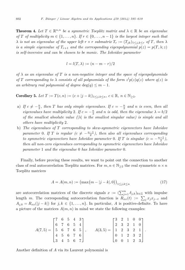
602 F. Bünger / Linear Algebra and its Applications 459 (2014) 595–619

Theorem 4. Let T ∈ Rn,n be a symmetric Toeplitz matrix and λ ∈ R be an eigenvalue

of T of multiplicity m ∈ {1, . . . , n}. If r ∈ {0, . . . , n − 1} is the largest integer such that λ is not an eigenvalue of the upper left r × r submatrix Tr := (Tjk)1≤j,k≤r of T , then λis a simple eigenvalue of Tr+1 and the corresponding eigenpolynomial p(z) = p(T, λ; z)is self-inversive and can be chosen to be monic. The Iohvidov parameter

l = l(T, λ) := (n−m− r)/2

of λ as an eigenvalue of T is a non-negative integer and the space of eigenpolynomials of T corresponding to λ consists of all polynomials of the form zlp(z)q(z) where q(z) is an arbitrary real polynomial of degree deg(q) ≤ m − 1.

Corollary 5. Let T := T (c, n) := (c + |j − k|)1≤j,k≤n, c ∈ R, n ∈ N≥3.

a) If c �= −n2 , then T has only simple eigenvalues. If c = −n

2 and n is even, then all eigenvalues have multiplicity 2. If c = −n

2 and n is odd, then the eigenvalue λ = b/2of the smallest absolute value (|λ| is the smallest singular value) is simple and all others have multiplicity 2.

b) The eigenvalues of T corresponding to skew-symmetric eigenvectors have Iohvidov parameter 0. If T is regular (c �= −n−1

2 ), then also all eigenvalues corresponding to symmetric eigenvectors have Iohvidov parameter 0. If T is singular (c = −n−1

2 ), then all non-zero eigenvalues corresponding to symmetric eigenvectors have Iohvidov parameter 1 and the eigenvalue 0 has Iohvidov parameter 0.

Finally, before proving these results, we want to point out the connection to another class of real autocorrelation Toeplitz matrices. For m, n ∈ N≥2 the real symmetric n ×n

Toeplitz matrices

A = A(m,n) :=(max

(m− |j − k|, 0

))1≤j,k≤n

(17)

are autocorrelation matrices of the discrete signals x := (∑m

j=1 δj,k)k∈Z with impulse length m. The corresponding autocorrelation function is Rxx(t) :=

∑j xjxj−t and

Aj,k = Rxx(|j − k|) for j, k ∈ {1, . . . , n}. In particular, A is positive-definite. To have a picture of the matrices A(m, n) in mind we state the following examples:

A(7, 5) =

⎡⎢⎢⎢⎢⎣

7 6 5 4 36 7 6 5 45 6 7 6 54 5 6 7 63 4 5 6 7

⎤⎥⎥⎥⎥⎦ , A(3, 5) =

⎡⎢⎢⎢⎢⎣

3 2 1 0 02 3 2 1 01 2 3 2 10 1 2 3 20 0 1 2 3

⎤⎥⎥⎥⎥⎦ .

Another definition of A via its Laurent polynomial is

F. Bünger / Linear Algebra and its Applications 459 (2014) 595–619 603

Aj,k = 12π

π∫−π

p(eiθ

)p(e−iθ

)e−i(j−k)θ dθ, j, k ∈ {1, . . . , n}

where p(z) := zm−1z−1 =

∑m−1k=0 zk and i :=

√−1. The matrix A is non-negative and

irreducible since its graph is strongly connected as Aj,j−1 = Ak,k+1 = m − 1 �= 0 for j = 2, . . . , n and k = 1, . . . , n − 1. Hence, by the Perron–Frobenius Theorem, the largest eigenvalue of A is simple. For m ≥ n − 1, we have A(m, n) = T (m, −1, n) and therefore Theorem 2 implies, since m �= n

2 , that actually all eigenvalues of A(m, n) are simple. For m < n − 1, repeated zeros occur in the upper right and lower left corner of A(m, n). Thus, for growing n and constant m a band structure with bandwidth m −1 is build out. In this case the eigenvalues of A(m, n) are not simple in general. For example, symbolic computations suggest that the matrices A(m, m(m −1)) for m ≥ 4 have the eigenvalue 1of multiplicity 2�m

2 � − 1.7 On the other hand, numerical simulations support

Conjecture 6. The smallest eigenvalue of A is simple.

To the authors knowledge the interesting class of integral, symmetric, positive defi-nite, non-negative, and irreducible Toeplitz matrices A(m, n) was explicitly treated for m ≤ n− 1 only by L. Rehnquist [12] who made an approach to compute the inverses. Since the class A(m, n) has so many structural properties and such a tempting simple pattern from the purely matrix theoretical point of view, we hope to encourage further research especially on its spectrum.

2. Proof of Theorem 1

For small dimensions n ∈ {1, 2} the assertion is easily checked and we may there-fore assume n ≥ 3 in the sequel. Define A := T (0, 1, n) = (|j − k|)1≤j,k≤n, and 1n := (1, . . . , 1)t ∈ R

n. Then, T = A + c1n1tn is simply a rank-1 update of the ma-

trix A. The inverse B := A−1 = (bjk)1≤j,k≤n and the determinant of A were derived by Fiedler, see [13, pp. 31, 32]:

bjk =

⎧⎪⎪⎪⎪⎪⎪⎨⎪⎪⎪⎪⎪⎪⎩

− n−22(n−1) if j = k ∈ {1, n},

−1 if j = k ∈ {2, n− 1},12 if |j − k| = 1,

12(n−1) if (j, k) ∈ {(1, n), (n, 1)},0 otherwise,

detA = (−1)n−12n−2(n− 1). (18)

Thus,

7 Thanks to Prof. S.M. Rump, TU Hamburg-Harburg, for pointing out this regular behavior.

604 F. Bünger / Linear Algebra and its Applications 459 (2014) 595–619

A−1 = −12

⎡⎢⎢⎢⎢⎢⎣

1 − 1n−1 −1 − 1

n−1−1 2 −1

. . . . . . . . .−1 2 −1

− 1n−1 −1 1 − 1

n−1

⎤⎥⎥⎥⎥⎥⎦ . (19)

Using the Sherman–Morrison–Woodbury formula, cf. [7], with u := c1n and v := 1n

yields that T = A + uvt is invertible if and only if 1 + utA−1v �= 0, and in this case

T−1 = A−1 − A−1uvtA−1

1 + utA−1v. (20)

From (19), utA−1v = 2cn−1 and

A−1uvtA−1 = c(A−11n

)(1tnA

−1) = c

(n− 1)2

⎡⎢⎢⎢⎢⎢⎣

1 0 . . . 0 10 0 . . . 0 0...

......

......

0 0 . . . 0 01 0 . . . 0 1

⎤⎥⎥⎥⎥⎥⎦ . (21)

Therefore, T is invertible if and only if

c �= −n− 12 , (22)

and in this case

T−1 = A−1 − c

(n− 1)(2c + n− 1)E (23)

where E := (1, 0, . . . , 0, 1)t(1, 0, . . . , 0, 1) is the matrix with ones in the corners that ap-pears in (21). Formula (23) is equivalent to (1). Finally, (18) and the matrix determinant lemma give (2):

detT = det(A + utv

)=

(1 + vtA−1u

)detA

=(

1 + 2cn− 1

)(−1)n−12n−2(n− 1) = (−1)n−12n−2(2c + n− 1).

3. Proof of Theorem 2

We define

S := 2T−1 =

⎡⎢⎢⎢⎢⎢⎣

−1 + τ 1 τ

1 −2 1. . . . . . . . .

1 −2 1

⎤⎥⎥⎥⎥⎥⎦ (24)

τ 1 −1 + τ

F. Bünger / Linear Algebra and its Applications 459 (2014) 595–619 605

with τ := 12c+n−1 . We will determine the eigenvalues and eigenvectors of S which directly

correspond to those of T . The matrix S can be viewed as a tridiagonal Toeplitz matrix with four symmetrically perturbed corners. Yueh and Cheng [19] gave formulas for eigen-values and eigenvectors in the even more general case of tridiagonal Toeplitz matrices with all four corners arbitrarily perturbed.8 But they derive explicit formulas only for certain perturbations and only implicit ones otherwise. Therefore, we do not apply their results directly but use the symmetry of the matrix S for a reduction first. Since S is symmetric and centrosymmetric, that is JSJ = S, where J = Jn := (δn−j+1,k)1≤j,k≤n is the flip-matrix, we can conjugate S in a well-known fashion to obtain a block structure that corresponds to the so-called even and odd factors of the characteristic polynomial of S (see [2, Theorem 2], and also [15]). First, set m := �n

2 �, J := Jm and partition Sinto blocks

S =[A JBJ

B JAJ

]if n is even, (25)

S =

⎡⎣A s JBJ

st −2 stJ

B Js JAJ

⎤⎦ if n is odd (26)

where

A :=

⎡⎢⎢⎢⎢⎢⎣

−1 + τ 11 −2 1

. . . . . . . . .1 −2 1

0 1 −2

⎤⎥⎥⎥⎥⎥⎦ ∈ R

m,m, (27)

B :=

⎡⎢⎢⎢⎣

0 . . . 0 γ... . . . . . . 00 . . . . . .

...τ 0 . . . 0

⎤⎥⎥⎥⎦ ∈ R

m,m, (28)

γ := 1 if n is even, and γ := 0 if n is odd, and s := (0, . . . , 0, 1)t ∈ Rm if n is odd. Next,

define the orthogonal matrix

K := 1√2

[I −J

J I

]if n is even, (29)

K := 1√2

⎡⎣ I 0 −J

0√

2 0J 0 I

⎤⎦ if n is odd. (30)

8 Similarly, Jain [9] also considers Toeplitz matrices with arbitrarily perturbed four corners but he only investigates the positive definite ones among them in greater detail, the orthonormal basis of eigenvectors of which build his “sinusoidal family of unitary transforms”. He proves asymptotic equivalence of the members of this family and general connections to Markov processes but he does not compute or enclose eigenvalues and eigenvectors explicitly. Thus, his work is of minor relevance in our context.

606 F. Bünger / Linear Algebra and its Applications 459 (2014) 595–619

Finally, conjugate S with K to obtain

KSKt =[A− JB 0

0 JAJ + BJ

]if n is even, (31)

KSKt =

⎡⎣A− JB 0 0

0 −2√

2stJ0

√2Js JAJ + BJ

⎤⎦ if n is odd. (32)

The blocks are easily identified as

C = Cm := A− JB =

⎡⎢⎢⎢⎢⎢⎣

−1 11 −2 1

. . . . . . . . .1 −2 1

1 −2 − γ

⎤⎥⎥⎥⎥⎥⎦ ∈ R

m,m, (33)

D = Dm := JAJ + BJ =

⎡⎢⎢⎢⎢⎢⎣

−2 + γ 11 −2 1

. . . . . . . . .1 −2 1

1 −2 + δ

⎤⎥⎥⎥⎥⎥⎦ ∈ R

m,m

with δ := 1 + 2τ = 1 + 22c + n− 1 , (34)

E = Em+1 :=[

−2√

2stJ√2Js Dm

]

=

⎡⎢⎢⎢⎢⎢⎢⎢⎣

−2√

2√2 −2 1

1 −2 1. . . . . . . . .

1 −2 11 −2 + δ

⎤⎥⎥⎥⎥⎥⎥⎥⎦∈ R

m+1,m+1, n odd. (35)

Thus, in order to determine the eigenvalues and eigenvectors of S, by (31) and (32) we have to find those of the symmetric tridiagonal matrices Cm for even and odd n, Dm for even n and Em+1 for odd n.

3.1. Eigenvalues and eigenvectors of Cm

The matrices Cm and Dm can be viewed as tridiagonal Toeplitz matrices with per-turbed upper left and lower right corners. Eigenvalues and eigenvectors of such matrices were studied by da Fonseca [3], Kouachi [10], Willms [17], Yueh [18], and Yueh and Cheng [19]. Let

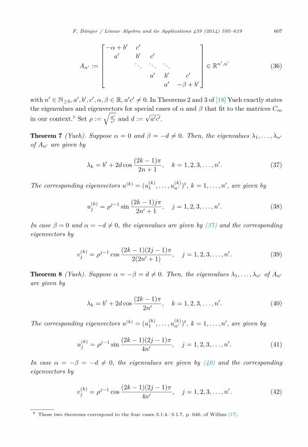
F. Bünger / Linear Algebra and its Applications 459 (2014) 595–619 607

An′ :=

⎡⎢⎢⎢⎢⎢⎣

−α + b′ c′

a′ b′ c′. . . . . . . . .

a′ b′ c′

a′ −β + b′

⎤⎥⎥⎥⎥⎥⎦ ∈ R

n′,n′(36)

with n′ ∈ N≥3, a′, b′, c′, α, β ∈ R, a′c′ �= 0. In Theorems 2 and 3 of [18] Yueh exactly states the eigenvalues and eigenvectors for special cases of α and β that fit to the matrices Cm

in our context.9 Set ρ :=√

a′

c′ and d :=√a′c′.

Theorem 7 (Yueh). Suppose α = 0 and β = −d �= 0. Then, the eigenvalues λ1, . . . , λn′

of An′ are given by

λk = b′ + 2d cos (2k − 1)π2n + 1 , k = 1, 2, 3, . . . , n′. (37)

The corresponding eigenvectors u(k) = (u(k)1 , . . . , u(k)

n′ )t, k = 1, . . . , n′, are given by

u(k)j = ρj−1 sin (2k − 1)jπ

2n′ + 1 , j = 1, 2, 3, . . . , n′. (38)

In case β = 0 and α = −d �= 0, the eigenvalues are given by (37) and the corresponding eigenvectors by

v(k)j = ρj−1 cos (2k − 1)(2j − 1)π

2(2n′ + 1) , j = 1, 2, 3, . . . , n′. (39)

Theorem 8 (Yueh). Suppose α = −β = d �= 0. Then, the eigenvalues λ1, . . . , λn′ of An′

are given by

λk = b′ + 2d cos (2k − 1)π2n′ , k = 1, 2, 3, . . . , n′. (40)

The corresponding eigenvectors u(k) = (u(k)1 , . . . , u(k)

n′ )t, k = 1, . . . , n′, are given by

u(k)j = ρj−1 sin (2k − 1)(2j − 1)π

4n′ , j = 1, 2, 3, . . . , n′. (41)

In case α = −β = −d �= 0, the eigenvalues are given by (40) and the corresponding eigenvectors by

v(k)j = ρj−1 cos (2k − 1)(2j − 1)π

4n′ , j = 1, 2, 3, . . . , n′. (42)

9 Those two theorems correspond to the four cases 3.1.4.–3.1.7, p. 646, of Willms [17].

608 F. Bünger / Linear Algebra and its Applications 459 (2014) 595–619

For even n the matrices Cm are the matrices Am with a′ = 1 = c′ = ρ = d, b′ = −2, and α = −1 = −β = −d so that its eigenvalues and eigenvectors are given by (40) and (42) with n′ = m. For odd n the matrices Cm are the matrices Am with a′ = 1 = c′ = ρ = d, b′ = −2, α = −1 = −d, and β = 0 so that its eigenvalues and eigenvectors are given by (37) and (39) with n′ = m. By (24) we simply have to invert the eigenvalues of S and hence of Cm and multiply them by two to obtain the eigenval-ues of T stated in (5). The corresponding skew-symmetric eigenvectors given in (6) are obtained from those of Cm by a skew-symmetric extension: a vector v ∈ R

m is skew-symmetrically extended to v̂ ∈ R

n by setting v̂j = vj for j = 1, . . . , m and v̂j = −vn+1−j

for j = m + 1, . . . , n which for odd n especially means v̂m+1 = 0. This finishes the proof of part a) of Theorem 2.

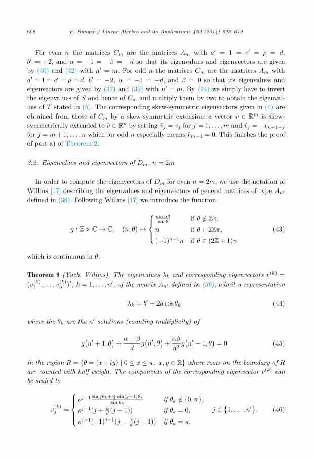
3.2. Eigenvalues and eigenvectors of Dm, n = 2m

In order to compute the eigenvectors of Dm for even n = 2m, we use the notation of Willms [17] describing the eigenvalues and eigenvectors of general matrices of type An′

defined in (36). Following Willms [17] we introduce the function

g : Z× C → C, (n, θ) �→

⎧⎪⎨⎪⎩

sin nθsin θ if θ /∈ Zπ,

n if θ ∈ 2Zπ,(−1)n−1n if θ ∈ (2Z + 1)π

(43)

which is continuous in θ.

Theorem 9 (Yueh, Willms). The eigenvalues λk and corresponding eigenvectors v(k) =(v(k)

1 , . . . , v(k)n′ )t, k = 1, . . . , n′, of the matrix An′ defined in (36), admit a representation

λk = b′ + 2d cos θk (44)

where the θk are the n′ solutions (counting multiplicity) of

g(n′ + 1, θ

)+ α + β

dg(n′, θ

)+ αβ

d2 g(n′ − 1, θ

)= 0 (45)

in the region R = {θ = (x + iy) | 0 ≤ x ≤ π, x, y ∈ R} where roots on the boundary of Rare counted with half weight. The components of the corresponding eigenvector v(k) can be scaled to

v(k)j =

⎧⎪⎪⎨⎪⎪⎩

ρj−1 sin jθk+αd sin(j−1)θk

sin θkif θk /∈ {0, π},

ρj−1(j + αd (j − 1)) if θk = 0,

ρj−1(−1)j−1(j − αd (j − 1)) if θk = π,

j ∈{1, . . . , n′}. (46)

F. Bünger / Linear Algebra and its Applications 459 (2014) 595–619 609

Applied to Dm, n even, we have n′ = m = n/2, a′ = 1 = c′ = ρ = d, b′ = −2, α = −γ = −1, β = −δ = −1 − 2

2c+n−1 . Therefore, (44), (45), and (46) reduce to

λk = 2(−1 + cos θk) (47)

0 = g(n′ + 1, θ

)− (1 + δ)g

(n′, θ

)+ δg

(n′ − 1, θ

)=

[g(n′ + 1, θ

)− g

(n′, θ

)]− δ

[g(n′, θ

)− g

(n′ − 1, θ

)](48)

v(k)j =

⎧⎪⎪⎨⎪⎪⎩

sin jθk−sin(j−1)θksin θk

= cos (2j−1)θk2

cos θk2

if θk /∈ {0, π},

1 if θk = 0,(−1)j−1(2j − 1) if θk = π,

1 ≤ j ≤ n. (49)

The function g fulfills the following trigonometric identity (cf. Willms[17, p. 645, no. (28)]):

g(j, θ) − g(j − 1, θ) =

⎧⎪⎪⎨⎪⎪⎩

cos (2j−1)θ2

cos θ2

if θ /∈ {0, π},1 if θ = 0,(−1)j−1(2j − 1) if θ = π,

j ∈ N. (50)

The regularity of S implies λk �= 0, so (48) does not have a root θk = 0 by (47). Thus, by (50) and (48) a θk is either a solution of

0 =cos (n+1)θ

2 − δ cos (n−1)θ2

cos θ2

= z−n2 · z

n+1 − δ(zn + z) + 1z + 1 , z := eiθ, (51)

in R\{0, π}, that is zk := eiθk ∈ C\{−1, 0, 1}, or θk = π and

0 = (−1)m(n + 1) − (−1)m−1(n− 1)δ ⇔ δ = −n + 1n− 1 . (52)

Consequently, the second case forces the m −1 remaining roots zk′ , k′ ∈ {1, . . . ,m}\{k}, to be solutions of

0 =zn+1 + n+1

n−1 (zn + z) + 1(z + 1)3 (53)

in R\{0, π}. Summing up, μk := 2bλ−1k = b

−1+cos θk , k = 1, . . . , m, are the eigenvalues of T stated in (7). The corresponding symmetric eigenvectors w(k) = (w(k)

1 , . . . , w(k)n )t

stated in (10) are the symmetric extensions of the v(k) given in (49) to the first mcomponents:

w(k) =√

2Kt

(0(k)

)=

(Jv(k)

(k)

)

v v

610 F. Bünger / Linear Algebra and its Applications 459 (2014) 595–619

Componentwise this means w(k)m+j = v

(k)j = w

(k)m+1−j , j = 1, . . . , m. This finishes the proof

of part b) of Theorem 2 for even n = 2m.

3.3. Eigenvalues and eigenvectors of Em+1, n = 2m + 1

Finally, we determine the eigenvalues and eigenvectors of the matrices E = Em+1 de-fined in (35) when n = 2m +1 is odd. It is somehow more convenient for us to transform E

further by conjugating with the diagonal matrix Q := diag(1, √

2, . . . , √

2 ) ∈ Rm+1, that

is we actually consider

F := Q−1EQ =

⎡⎢⎢⎢⎢⎢⎣

−2 21 −2 1

. . . . . . . . .1 −2 1

1 −2 + δ

⎤⎥⎥⎥⎥⎥⎦ (54)

instead of E. The matrix F differs from E only in the (1, 2)- and (2, 1)-entry where √

2 is replaced by 2 and 1 respectively. Let us fix an eigenvalue λ ∈ C of F with corresponding eigenvector u = (u1, . . . , un′) ∈ C

n′ , n′ := m +1. First we treat the case λ = −4. By (54), (Fu)j = −4uj for j = 1, . . . , n′−1 implies uj = (−1)j−1u1, j = 1, . . . , n′. Evaluating the last component of (Fu)j = −4uj yields (3 − δ)u1 = (Fu)n′ = −4un′ = 4u1 which means −1 = δ = 1 + 2

2c+n−1 , that is, c = −n2 . Thus, we see that the case λ = −4 is included

in (7) and the last line of (10) with θk = π and zk := eiθk = −1 being a double root of pn(δ; z) = zn+1 + zn + z + 1.

Next, for λ �= −4, we follow the arguments of Yueh and Cheng [19] in order to determine the eigenvalues and eigenvectors of F . The eigenvector u can be extended to a sequence (uj)j∈N0 ∈ C

N0 which fulfills the three-term recursion

uk−1 + (−2 − λ)uk + uk+1 = fk (55)

with boundary conditions

fk :=

⎧⎨⎩

−u2 if k = 1,−δun′ if k = n′,

0 else,(56)

and constraints

u0 = 0 = un′+1. (57)

Setting � := (δ1,j)j∈N0 = (0, 1, 0, . . .) ∈ CN0 and c := (c, c, . . .) ∈ C

N0 for c ∈ C the recursion (55) reads in sequence notation

(�

2 + (−2 − λ)� + 1)u = (u1 + f)� (58)

F. Bünger / Linear Algebra and its Applications 459 (2014) 595–619 611

where the product of two sequences a = (aj)j∈N0 and b = (bj)j∈N0 is the convolution a ∗ b = c = (cj)j∈N0 , cj :=

∑jk=0 akbj−k. Eq. (58) has the solution

u = (u1 + f)��2 + (−2 − λ)� + 1

= 1√ω

(1

γ− − �− 1

γ+ − �

)(cu1 + f)�

= 2i√ω

(sin jθ)j∈N0(cu1 + f) (59)

where

γ± := 2 + λ±√ω

2 = e±iθ = cos θ ± i sin θ, θ ∈ C, Re θ ∈ [0, π], (60)

are the roots of the quadratic polynomial z2 + (−2 − λ)z + 1 ∈ C[z] and

√ω :=

√(2 + λ)2 − 4 = 2i sin θ �= 0

as 0 �= λ �= −4. Evaluating (59) componentwise yields

uj = 2i√ω

(u1 sin jθ − u2 sin(j − 1)θ −H

(j − n′)δun′ sin

(j − n′)θ) (61)

for j ≥ 1 where H is the Heaviside-function, that is H(x) = 0 if x ≤ 0, and H(x) = 1if x > 0. Let us first consider the case n = 2m + 1 = m + n′ ≥ 5, that is n′ ≥ 3. Then, 2, n′, n′ + 1 are distinct and (61) evaluated for these values supplies

u2

u1= sin 2θ

2 sin θ= cos θ (62)

un′

u1sin θ = sinn′θ − u2

u1sin

(n′ − 1

)θ (63)

0 = sin(n′ + 1

)θ − u2

u1sinn′θ − δ

un′

u1sin θ. (64)

Note that u1 (and un′) cannot be zero, since otherwise (55) would imply u = 0. If n = 3, that is n′ = 2, (63) and (64) still hold. But (63) becomes

u2

u1sin θ = sin 2θ − u2

u1sin θ ⇔ u2

u1= sin 2θ

2 sin θ= cos θ. (65)

Thus, (62) also holds. Inserting (63) into (64) and replacing u2u1

by the right side of (62)gives

0 = sin(n′ + 1

)θ − u2

u1sinn′θ − δ

(sinn′θ − u2

u1sin

(n′ − 1

)θ

)

= sin(n′ + 1

)θ − cos θ sinn′θ − δ

(sinn′θ − cos θ sin

(n′ − 1

)θ)

612 F. Bünger / Linear Algebra and its Applications 459 (2014) 595–619

= 12(sin

(n′ + 1

)θ − sin

(n′ − 1

)θ − δ

(sinn′θ − sin

(n′ − 2

)θ))

=(cosn′θ − δ cos

(n′ − 1

)θ)sin θ.

Since sin θ �= 0, we obtain the following necessary condition for θ:

0 = cosn′θ − δ cos(n′ − 1

)θ. (66)

By substituting z := eiθ we may convert this trigonometric equation to a polynomial one:

0 = z2n′+ 1 − δ

(z2n′−1 + z

)= zn+1 + 1 − δ

(zn + z

)= pn(δ; z). (67)

Thus, the eigenvalues of F (which are clearly those of E) are described by the roots of the polynomial pn(δ; z) in exactly the same way as those of Dm in the preceding subsection. Hence, the eigenvalues of T corresponding to symmetric eigenvectors are also for odd nthose stated in (7). By (61) and (62) the components of the eigenvector u can be scaled to

uj = sin jθ − u2

u1sin(j − 1)θ = sin jθ − cos(θ) sin(j − 1)θ

= sin jθ − 12(sin(j − 2)θ + sin jθ

)= 1

2(sin jθ − sin(j − 2)θ

)= cos(j − 1)θ sin θ.

The corresponding extended eigenvector of S and T can be chosen as

w := 1sin θ

Kt

(0Qu

)=

(cos|m + 1 − j|θ

)j=1,...,n

which establishes the last line of (10) and finishes the proof of Theorem 2.

4. Proof of Theorem 3

We use a continuity argument to prove Theorem 3. Consider a small perturbation c̃of c. Then, T̃ := T (c̃, n) is regular and its eigenvalues and eigenvectors are described in Theorem 2. By continuity they will converge for c̃ → c to those of T . First note that the skew-symmetric eigenvectors and corresponding eigenvalues of T̃ given in Theorem 2 a) do not depend on c̃, so that they coincide with those of T which proves part a) of Theorem 3.

The quantity δ̃ := 1 + 22c̃+n−1 converges to ±∞ for c̃ → c = −n−1

2 . Thus, the roots of the polynomial

pn(δ; z) :={

zn+1−δz(zn−1+1)+1z+1 if n is even,

n+1 n−1

z − δz(z + 1) + 1 if n is odd,

F. Bünger / Linear Algebra and its Applications 459 (2014) 595–619 613

defined in (8) converge to those of

pn(±∞; z) :={

z(zn−1+1)z+1 if n is even,

z(zn−1 + 1) if n is odd

which are 0 and exp(iθk), θk := (2k−1)πn−1 , k ∈ {1, . . . , n − 1}. For k ∈ {1, . . . , n−m− 1}

we have θk ∈ R = (0, π] ∪ iR>0 ∪ π + iR>0. Inserting these θk into (7) and (10) gives the first n −m − 1 symmetric eigenvectors and corresponding eigenvalues stated in (15)and (16).

Finally, the remaining root z = 0 may formally be written as 0 = exp(iθl), l := n −m, with θl := i · (+∞). The corresponding perturbed θ̃l ∈ R converging to θl supplies an

eigenvector w̃(l) = (w̃(l)1 , . . . , w̃(l)

n )t ∈ Rn with components given in (10):

w̃(l)m+j = w̃

(l)l+1−j =

{cos(j − 1

2 )θ̃l if n is even,cos(j − 1)θ̃l if n is odd,

1 ≤ j ≤ l.

Scaling the first and last component of w̃(l) to 1 by dividing through w̃(l)1 yields

limθ̃l→θl

1w̃

(l)1

w̃(l)m+j = lim

θ̃l→θl

1w̃

(l)1

w̃(l)l+1−j = lim

θ̃l→θl

⎧⎪⎨⎪⎩

cos(j− 12 )θ̃l

cos(l− 12 )θ̃l

if n is even,

cos(j−1)θ̃lcos(l−1)θ̃l

if n is odd,= δj,l

for j ∈ {1, . . . , l}. Thus, the vector u := (1, 0, . . . , 0, 1)t ∈ Rn is contained in the kernel

of T which of course could have been verified directly without the above derivation: (Tu)j = Tj,1 + Tj,n = c + |j − 1| + c + |n − j| = 2c + n − 1 = 0. This finishes the proof of part b) of Theorem 3.

5. Proof of Corollary 5

a) If T is singular, then Theorem 3 shows that all eigenvalues are simple, so that the assertion holds in this case. Thus, we may assume that T is regular. By Theorem 2 the eigenvalues corresponding to skew-symmetric eigenvectors are pairwise distinct and the same holds true for the eigenvalues corresponding to symmetric eigenvectors by P1)–P8). Indeed, this fact can be deduced directly without any special knowledge on the eigen-values of T from the tridiagonal matrices Cm, Dm, and Em defined in the proof of Theorem 2 (cf. (33)–(35)) which of course only have simple eigenvalues. Thus, if we as-sume that T has a multiple eigenvalue λ, then the corresponding eigenspace necessarily contains symmetric and skew-symmetric eigenvectors.10

10 Indeed, this is a priori known by a result of Delsarte and Genin [4, Theorem 8, p. 204], which says that an eigenspace of dimension d of a real symmetric Toeplitz matrix possesses a basis consisting of d

2 �(or � d

2 ) symmetric and � d2 (or d

2 �) skew-symmetric eigenvectors, that is, the numbers of symmetric and skew-symmetric basis eigenvectors split the eigenspace dimension as evenly as possible.

614 F. Bünger / Linear Algebra and its Applications 459 (2014) 595–619

But then (5) and (7) imply λ = (−1 + cos θ)−1 where θ = (2k−1)πn for some

k ∈ {1, . . . ,m} satisfies

0 = cos (n + 1)θ2 − δ cos (n− 1)θ

2 = (1 + δ)(−1)k sin π

2n.

We see that this is only possible for δ = −1, that is c = −n2 . By P3) the eigenvalues of T

corresponding to symmetric eigenvectors

μk =(−1 + cos (2k − 1)π

n

)−1

, k = 1, . . . , n−m,

coincide with those corresponding to skew-symmetric eigenvectors (cf. (5)) with one exception where n = 2m + 1 is odd and k = n −m = m + 1 when μm+1 = −b/2 is the eigenvalue of the smallest absolute value.

b) By (6) the first component of a skew-symmetric eigenvector v(k) is v(k)1 = cos (2k−1)π

2n ,which is distinct from 0 for k ∈ {1, . . . , m}. By Theorem 4 the Iohvidov parameter of the corresponding eigenvalue is 0. If T is singular, then by (15) the first two components of a symmetric eigenvector w(k), k ∈ {1, . . . ,m}, are

w(k)1 =

{cos (2k−1)π

2 = 0 if 1 ≤ k ≤ n−m− 1,1 if k = n−m,

w(k)2 =

{(−1)k−1 sin (2k−1)π

n−1 �= 0 if 1 ≤ k ≤ n−m− 1,0 if k = n−m.

Since by a) all eigenvalues are simple, this implies that the non-zero eigenvalues of Tcorresponding to symmetric eigenvectors have Iohvidov parameter one and the eigenvalue μ = 0 with eigenvector (1, 0, . . . , 0, 1)t has Iohvidov parameter zero.

Now suppose that T is regular. Then, by (10) the first component of a symmetric eigenvector w = (w1, . . . , wn)t can be found as

w1 = wn ={

cos (n−1)θ2 if θ �= π,

(−1)m−1(n− 1) if n is even and θ = π,

for some θ ∈ R := (0, π] ∪ iR>0 ∪ π + iR>0 satisfying

cos(n + 1)θ2 − δ cos(n− 1)θ2 = 0, δ = 1 + 2/(2c + n− 1).

Thus, if θ = π, then clearly w1 �= 0. But this also holds for θ �= π since otherwise θmust have the form θ = 2k−1

n−1 π for some k ∈ {1, . . . , n−m− 1} which by (15) [or P4)] corresponds to singular T (formally δ = ±∞) treated before. Thus, again w1 �= 0 shows that the Iohvidov parameter of the corresponding eigenvalue is 0.

F. Bünger / Linear Algebra and its Applications 459 (2014) 595–619 615

Acknowledgement

I thank Professor A. Böttcher from Chemnitz University of Technology for valuable hints and comments that led to improvements of this paper.

Appendix A

This appendix contains the rather technical proofs of P1)–P8), P7′), P8′), (11), (12). The roots of pn(δ; z) are those of qn(δ; z) := zn + 1 − δ(zn + z) where for even n the multiplicity of the root −1 is reduced by one. The roots of qn(δ; z) correspond to those of the trigonometric polynomial

Qn(δ; θ) := e−i(n+1) θ2 qn

(δ; eiθ

)= cos (n + 1)θ

2 − δ cos (n− 1)θ2 .

Actually, we may view qn(δ; z) (and Qn(δ; θ)) as a homotopy of (trigonometric) polyno-mials which causes the distinguished cases for δ. To make this clear, let us look at the polynomials

qn(0; z) = zn+1 + 1

qn(1; z) = zn+1 − zn − z + 1

qn(−1; z) = zn+1 + zn + z + 1

qn(±∞; z) := zn + z

with corresponding trigonometric polynomials

Qn(0; θ) = cos (n + 1)θ2

Qn(1; θ) = cos (n + 1)θ2 − cos (n− 1)θ

2 = −2 sin nθ

2 sin θ

2

Qn(−1; θ) = cos (n + 1)θ2 + cos (n− 1)θ

2 = 2 cos nθ2 cos θ2

Qn(±∞; θ) := e−i(n+1) θ2 qn

(±∞; eiθ

)= cos (n− 1)θ

2 .

Now for δ ∈ [0, 1], qn(δ, z) is a homotopy of qn(0; z) to qn(1; z), and for δ ∈ [−1, 0], qn(δ, z) is a homotopy of qn(0; z) to qn(−1; z). If δ ∈ [1, +∞], δ−1qn(δ, z) is a homotopy of qn(1; z) to qn(±∞; z), and finally, if δ ∈ [−∞, −1], δ−1qn(δ, z) is a homotopy of qn(−1; z) to qn(±∞; z). The same holds true for the trigonometric polynomials. The whole thing now is to establish the stated inclusions for the zeros of pn(δ; z) by those of the polynomials qn(0; z), qn(1; z), qn(−1; z), qn(±∞; z) which are immediately deduced from the trigonometric representations given above. If we define

616 F. Bünger / Linear Algebra and its Applications 459 (2014) 595–619

θ(0)k := 2k − 1

n + 1 π, k = 1, . . . , n−m,

θ(1)k := 2(k − 1)

nπ, k = 1, . . . , n−m,

θ(−1)k := 2k − 1

nπ, k = 1, . . . , n−m,

θ(±∞)k := 2k − 1

n− 1 π, k = 1, . . . , n−m− 1,

then θ(δ)k ∈ [0, π] and Q(δ, ±θ

(δ)k ) = 0 for δ ∈ {0, 1, −1, ±∞} and the given k. The range

of the k is already chosen such that for even n the root z = −1 that corresponds to θ = π

is neglected. This proves P1) to P4). For d) note that z = 0 clearly is the remaining root of qn(±∞; z) = z(zn−1 + 1). This case corresponds to singular matrices T (c, n) as already shown in the proof of Theorem 3. Define the open intervals

I(0,1)k :=

(θ(1)k , θ

(0)k

), k = 1, . . . , n−m,

I(−1,0)k :=

(θ(0)k , θ

(−1)k

), k = 1, . . . , n−m,

I(1,∞)k :=

(θ(±∞)k−1 , θ

(1)k

), k = 2, . . . , n−m,

I(−∞,−1)k :=

(θ(−1)k , θ

(±∞)k

), k = 1, . . . , n−m− 1.

Then, it is routine to check that none of the angles θ(±∞)j , j = 1, . . . , n − m − 1, is

contained in any of these intervals. But this means that the function

f(θ) := Qn(0; θ)Qn(±∞; θ) =

cos (n+1)θ2

cos (n−1)θ2

(68)

restricted to any of those intervals is well defined and continuous and can be continuously extended to the boundaries in those cases where they differ from the zeros θ(±∞)

k of the

denominator Qn(±∞; θ). Since f(θ(1)k ) = 1, f(θ(0)

k ) = 0 the intermediate value theorem

yields (0, 1) ⊆ f(I(0,1)k ). Thus, for each δ ∈ (0, 1) there is a θk = θk(δ) ∈ I

(0,1)k such that

f(θk) = δ which is equivalent to Qn(δ, θk) = 0. This proves P5) and analogously P6). In

the same way f(θ(1)k ) = 1 and lim

θ↓θ(±∞)k−1

f(θ) = +∞ imply (1, +∞) ⊆ f(I(1,∞)k ). Hence,

again there exists for each δ ∈ (1, +∞) a θk = θk(δ) ∈ I(1,∞)k such that f(θk) = δ so that

Qn(δ, θk) = 0. This proves the inclusions for θk stated in P7) for k = 2, . . . , n −m and analogously the inclusions for θk given in P8) for k = 1, . . . , n −m − 1. For δ ∈ (1, +∞)we have qn(δ; 0) = 1 > 0 > 2(1 − δ) = qn(δ; 1). Using the intermediate value theo-rem we find the last remaining root z1 ∈ (0, 1) to prove P7). Next, we prove P8). Let δ ∈ (−∞, −1) and suppose that n is odd, then qn(δ; −1) = 2(1 − |δ|) < 0 < 1 = pn(δ; 0)and again the intermediate value theorem supplies the missing root zn−m ∈ (−1, 0). Now suppose that n is even, then all coefficients of qn(δ; z) = zn+1 + |δ|zn + |δ|z + 1are positive, whence qn(δ; z) does not have positive real roots. The coefficients of

F. Bünger / Linear Algebra and its Applications 459 (2014) 595–619 617

qn(δ;−z) = −zn+1 + |δ|zn − |δ|z + 1 change their signs three times, so that by Descartes rule of signs qn(δ; z) has either three or one negative real roots where −1 is clearly one of them. Looking at the derivative q′n(δ; z) = (n + 1)zn − δ(nzn−1 + 1) we see

q′n(δ;−1) = (n + 1) + δ(n− 1)

⎧⎪⎨⎪⎩

< 0 if δ < −n+1n−1 ,

= 0 if δ = −n+1n−1 ,

> 0 if δ > −n+1n−1 .

Thus, if δ < −n+1n−1 , then qn(δ; z) assumes negative values in (−1, 0) and, since

qn(δ, 0) = 1 > 0, there must be at least one root zm = zn−m in (−1, 0). By the preceding considerations z−1

m , −1, zm are all real roots of qn(δ; z). If δ = −n+1n−1 , then z = −1

is a three-fold root of qn(δ, z) as already mentioned in Theorem 2. If δ > −n+1n−1 , then

qn(δ; −1) = 0, q′n(δ; −1) > 0, and qn(δ; 0) = 1 > 0 imply that qn(δ; z) must have an even number 2ν, ν ∈ N0, of roots in (−1, 0) counting multiplicities. Since qn(δ; −1) is self-inversive, it must have the same number of roots in (−∞, −1), so that we obtain 4ν + 1 real roots overall. But we already found n − 2 non-real roots of qn(δ; −1) on the complex unit circle, whence ν = 0. Since cos n−1

2 θ does not have a zero in (n−1n π, π), the

function f(θ) (cf. (68)) is well defined and continuous and can be continuously extended to the boundaries using L’Hospital’s rule at the right boundary:

f

(n− 1n

· π)

= −1 and f(π) := limθ→π

cos (n+1)θ2

cos (n−1)θ2

= limθ→π

(n + 1) sin (n+1)θ2

(n− 1) sin (n−1)θ2

= −n + 1n− 1 .

Thus, δ ∈ (−n+1n−1 , −1) ⊆ f((n−1

n π, π)) finally supplies the remaining root θm ∈ (n−1n π, π)

with f(θm) = δ, that is Qn(δ, θm) = 0 proving P8).In all inclusions given in P5) to P8) we found that the θk = θk(δ) are implicitly defined

functions on the given intervals by the equation f(θk(δ)) = δ. Building derivatives on both sides yields

1 =−n+1

2 sin (n+1)θk(δ)2 cos (n−1)θk(δ)

2 + n−12 cos (n+1)θk(δ)

2 sin (n−1)θk(δ)2

cos2 (n−1)θk(δ)2

· θ′k(δ)

0 < cos2 (n− 1)θk(δ)2 =

(−n + 1

2 sin (n + 1)θk(δ)2 cos (n− 1)θk(δ)

2

+ n− 12 cos (n + 1)θk(δ)

2 sin (n− 1)θk(δ)2

)θ′k(δ)

=(−n + 1

2 sin (n + 1)θk(δ)2 + n− 1

2 δ sin (n− 1)θk(δ)2

)· θ′k(δ) cos (n− 1)θk(δ)

2 .

This shows θ′k(δ) �= 0 in the given open intervals and also proves (11). Hence, θk(δ)depends monotonically on δ. From P1) to P4) where the boundary values of δ were considered, we see that the real θk(δ) and the real z1 = z1(δ) [case P7)], zn−m = zn−m(δ)

618 F. Bünger / Linear Algebra and its Applications 459 (2014) 595–619

[case P8)] are monotonically decreasing functions of δ. Finally, we prove (12). For δ close to but distinct from 1 we compute using the chain rule and (11):

(cos θ1(δ)

)′ = −θ′1(δ) sin θ1(δ) =−sin θ1(δ) cos (n−1)θ1(δ)

2

−n+12 sin (n+1)θ1(δ)

2 + n−12 δ sin (n−1)θ1(δ)

2

.

Since limδ→1 θ1(δ) = 0, both the numerator and denominator of the above fraction converge to 0 for δ → 1 so that we can apply L’Hospital’s rule to compute the limit:

(−sin θ1(δ) cos (n−1)θ1(δ)2 )′

(−n+12 sin (n+1)θ1(δ)

2 + n−12 δ sin (n−1)θ1(δ)

2 )′

=(−cos θ1(δ) cos (n−1)θ1(δ)

2 + n−12 sin θ1(δ) sin (n−1)θ1(δ)

2 )θ′1(δ)(−(n+1

2 )2 cos (n+1)θ1(δ)2 + (n−1

2 )2δ cos (n−1)θ1(δ)2 + n−1

2θ′1(δ)

sin (n−1)θ1(δ)2 )θ′1(δ)

.

Since limδ→1|θ′1(δ)| = +∞ by (11), the above fraction converges for δ → 1 to −1

−(n+12 )2+(n−1

2 )2 = 1n proving (12). Finally, we prove P7′) and P8′). Set

q(z) := zn+1 − δzn − δz + 1.

P7′) Since δ > 1, Cauchy’s bound for the moduli of the roots of q(z) is 1 + δ. Hence, q(δ) = δ2 − 1 < 0 and limx→∞ q(x) = +∞ imply δ < ζ ≤ δ + 1 which proves P7′) if ρ = 1. If ρ =

√δ2 − 1 < 1, then

q(δ + ρ) = ρ(δ + ρ)n − δ(δ + ρ) + 1 ≥ ρ(δ + ρ) − δ(δ + ρ) + 1 = 0

also shows δ < ζ ≤ δ + ρ.P8′) If n is odd, then pn(δ; −z) = zn+1 − |δ|zn − |δ|z + 1 = pn(|δ|; z) and the as-

sertion follows from P7′). Now suppose that n ≥ 3 is even. If δ < −2, then ρ = 1, |δ + ρ| = |δ| − 1 > 1, and

q(δ + ρ) = (δ + 1)n − δ(δ + 1) + 1 >(|δ| − 1

)3 − δ(δ + 1) + 1

= |δ|3 − 4|δ|2 + 4|δ| + 1 ≥ 0 > δ2 − 1 = q(δ).

This implies ζ ∈ (δ, δ + ρ) = (δ, δ + 1).If −2 ≤ δ < −n+1

n−1 , then ρ = |δ + 1| = −δ − 1, δ + ρ = −1, and for

p(z) := pn(δ; z) = q(z)/(z + 1) = zn +n−1∑j=1

(−z)j + 1

we have p(δ + ρ) = p(−1) = 2 + (n − 1)(1 + δ) < 0 < p(δ) = (δ2 − 1)/(δ + 1). Again, this implies ζ ∈ (δ, δ + ρ) = (δ, −1).

F. Bünger / Linear Algebra and its Applications 459 (2014) 595–619 619

References

[1] M. Bogoya, A. Böttcher, S. Grudsky, Eigenvalues of Hermitian Toeplitz matrices with polynomially increasing entries, J. Spectr. Theory 2 (2012) 267–292.

[2] A. Cantoni, P. Butler, Eigenvalues and eigenvectors of symmetric centrosymmetric matrices, Linear Algebra Appl. 13 (1976) 275–288.

[3] C.M. da Fonseca, The characteristic polynomial of some perturbed tridiagonal k-Toeplitz matrices, Appl. Math. Sci. 1 (2) (2007) 59–67.

[4] P. Delsarte, Y. Genin, Spectral properties of finite Toeplitz matrices, in: Lecture Notes in Control and Inform. Sci., vol. 58, Springer, 1984, pp. 194–213.

[5] P. Delsarte, Y. Genin, Y. Kamp, Parametric Toeplitz systems, Circuits Systems Signal Process. 3 (2) (1984) 207–223.

[6] R.T. Gregory, D.L. Karney, A Collection of Matrices for Testing Computational Algorithms, Wiley–Interscience, New York, London, Sydney, Toronto, 1969.

[7] G.H. Golub, C.F. Van Loan, Matrix Computations, third ed., The Johns Hopkins University Press, Baltimore, London, 1996.

[8] I.S. Iohvidov, Hankel and Toeplitz Matrices and Forms, Birkhäuser, 1982.[9] A.K. Jain, A sinusoidal family of unitary transforms, IEEE Trans. Pattern Anal. Mach. Intell.

PAMI-1 (4) (1979) 356–365.[10] S. Kouachi, Eigenvalues and eigenvectors of tridiagonal matrices, Electron. J. Linear Algebra 15

(2006) 115–133.[11] M.H. Lietzke, R.W. Stoughton, M.P. Lietzke, A comparison of several methods for inverting large

symmetric positive definite matrices, Math. Comp. 18 (1964) 449–456.[12] L. Rehnquist, Inversion of certain symmetric band matrices, BIT 12 (1) (1972) 90–98.[13] J. Todd, The problem of error in digital computation, in: L.B. Rall (Ed.), Error in Digital Compu-

tation, vol. I, John Wiley & Sons, Inc., 1965, pp. 3–41.[14] W.F. Trench, Spectral distribution of generalized Kac–Murdock–Szegö matrices, Linear Algebra

Appl. 347 (2002) 251–273.[15] W.F. Trench, Characterization and properties of matrices with generalized symmetry or skew sym-

metry, Linear Algebra Appl. 377 (2004) 207–218.[16] J. Westlake, A Handbook of Numerical Matrix Inversion and Solution of Linear Equations, John

Wiley & Sons, Inc., 1968.[17] A.R. Willms, Analytic results for the eigenvalues of certain tridiagonal matrices, SIAM J. Matrix

Anal. Appl. 30 (2) (2008) 639–656.[18] Wen-Chyan Yueh, Eigenvalues of several tridiagonal matrices, Appl. Math. E-Notes 5 (2005) 66–74.[19] Wen-Chyan Yueh, Sui Sun Cheng, Explicit eigenvalues and inverses of tridiagonal Toeplitz matrices

with four perturbed corners, ANZIAM J. 49 (2008) 361–387.