Reshetov LA New representations of the Moore–Penrose inverse of 2 × 2 block matrices

Contents lists available at ScienceDirect

Linear Algebra and its Applications

www.elsevier .com/locate/ laa

New representations of the Moore–Penrose inverse

of 2 × 2 block matrices<

Zi- ong Yan

Department of Information and Mathematics, Yangtze University, Jingzhou, Hubei, China

A R T I C L E I N F O A B S T R A C T

Article history:

Received 18 February 2012

Accepted 21 August 2012

Submitted by V. Mehrmann

AMS classification:

15A15

15A23

Keywords:

Moore–Penrose inverse

Full rank factorization

Banachiewicz–Schur forms

This paper presents a full rank factorization of a 2 × 2 block matrix

without any restriction. Applying this factorization, we obtain an

explicit representation of the Moore–Penrose inverse in terms of

four individual blocks of the partitioned matrix, which simplifies

results of Hung and Markham (1975) [12], and Miao (1991) [16]. We

also derive some important coincidence theorems, including in the

expressions of the Moore–Penrose inverse of a sum of matrices. All

these results extend earlier works by various authors.

© 2012 Elsevier Inc. All rights reserved.

1. Introduction

Matrix algebra problems have emerged from the main stream of the least square estimation in the

general Gauss–Markovmodels, particularly from the theory of constrained linearmodels (for example,

see Baksalary [1]). One of such problems concerns the generalized inverse of a 2 × 2 block matrix

A =⎛⎝A B

C D

⎞⎠ . (1)

This paper generalizes and simplifies previous results by Huan and Markham [12], and Miao [16]

about an explicit representation of the Moore–Penrose inverse of A, in terms of the individual blocks

A, B, C,D. The main result is derived using a full rank factorization of A (without any restrictions)

< The research foundation of Education Bureau of Hubei Province, PR China (Grant No. D20111305).E-mail address: [email protected]

0024-3795/$ - see front matter © 2012 Elsevier Inc. All rights reserved.

Z

Linear Algebra and its Applications 456 (2014) 3–15

http://dx.doi.org/10.1016/j.laa.2012.08.014

Available online 23 September 2012

http://www.sciencedirect.com/science/journal/00243795

www.elsevier.com/locate/laa

mailto:[email protected]



http://crossmark.crossref.org/dialog/?doi=10.1016/j.laa.2012.08.014&domain=pdf

that follows from previous results by Marsaglia and Styan [14], and Meyer [17]. The paper presents

the general case (see below Theorem 3.6) as well as special cases in which the formulas simplify

considerably.

There are a great deal of works for the generalized inverse of A. In a sequence of early papers

[3,4,10,17,27], it has been of interest to derive a general expression for conditional or 1-inverses and

reflexive or 1–2 inverses of A in terms of the individual blocks without any restrictions imposed.

Various other generalized inverses have also been researched by a lot of researchers, for example,

Noble [21], Pringle and Rayner [24], Marsaglia and Styan [14], Hall [9], Wang and Chen [31], Miao

[15], and the references therein. Very recently, several generalized inverses of partitionedmatrices for

positive semidefinite matrices were discussed by Groß [8], Cegielski [7], Baksalary and Styan [2], Tian

and Takane [30], and etc. Most works in literature concerning representations for the Moore–Penrose

inverses of partitioned matrices were carried out under certain restrictions on their blocks, although

twogeneral expressions for theMoore–Penrose inverseswithout any restriction imposedon theblocks

were presented in Hung and Markham [12], and Miao [16].

It is convenient to lead to an explicit formula for the Moore–Penrose inverse of a matrix by its full

rank factorization. Arising from different block decompositions of rectangular matrices, it has been

used in computing the Moore–Penrose inverses of partitioned matrices by Nobel [20], Tewarson [29],

Robert [28], Zlobec [32], Lancaster and Tismenetsky [13], Milovanovic and Stanimirovic [18], and oth-

ers. Main advantages of block representations are their simply derivation, computation and possibility

of natural generalization. These methods, however, could obtain useful explicit representations of the

generalized inverse only if the top-left block of A is invertible. Here we present a full rank factor-

ization of A without any restriction. The Moore–Penrose inverses of partitioned matrices with the

corresponding consequences, based on this full rank factorization, are discussed in this paper.

The outline of our paper is as follows. In Section 2, we present a full rank factorization ofA (without

any restriction) using previous results by Marsaglia and Styan [14], and Meyer [17]. Inspired by this

factorization,we extend the analysis to obtain an explicit representation of theMoore–Penrose inverse

ofA in Section 3. In Section 4, we discuss variants special formswith the corresponding consequences,

including Banachiewicz–Schur forms and some other recent extensions as well.

All matrices of this paper are over the complex field, and are not null without special situation. The

symbols A∗, r(A), R(A) andN(A) stand for the conjugate transpose, the rank, the column space and the

null space of a matrix A, respectively. A† = X denotes the Moore–Penrose inverse of A in [19,22,26]

satisfying

(a)AXA = A, (b)XAX = X, (c)(AX)∗ = AX, (d)(XA)∗ = XA. (2)

A full rank factorization of A is in form

A = FAGA, (3)

where FA and GA are of full rank. Any choice in (3) is acceptable throughout the paper, although this

factorization is not unique.

With the help of the full rank factorization and the Moore–Penrose inverse of a matrix, Piziak and

OdellSource [23] have popularized a structural view of a projection. A standard method of computing

projections begins by finding an orthonormal basis for the subspace. This is unnecessary, given a full

rank factorization (3), since the Moore–Penrose equations imply

(i) AA† = FAF†A is the projection onto R(A);

(ii) A†A = G†AGA is the projection onto R(A∗);

(iii) I − AA† = I − FAF†A is the projection onto N(A∗);

(iv) I − A†A = I − G†AGA is the projection onto N(A).

For brevity, PA = I − AA† and QA = I − A†A denote two orthogonal projections onto the spaces of

N(A∗) and N(A), respectively.

Z.-Z. Yan / Linear Algebra and its Applications 456 (2014) 3–154

2. The full rank factorization of a partitioned matrix

Let us start with a very useful lemma.

Lemma 2.1 (Marsaglia and Styan [14], Meyer [17]). Let

S = D − CA†B, E = PAB, W = CQA, R = PWSQE. (4)

Then

r(A, B) = r(A) + r(E), (5)

r

⎛⎝ A

C

⎞⎠ = r(A) + r(W), (6)

r

⎛⎝ 0 B

C D

⎞⎠ = r(B) + r(C) + r(PCDQB), (7)

r

⎛⎝ A B

C D

⎞⎠ = r(A) + r

⎛⎝ 0 E

W S

⎞⎠ (8)

= r(A) + r(E) + r(W) + r(R). (9)

Coming from two seminal papers of Marsaglia and Styan [14] and of Meyer [17], the fundamental

relations (5)–(8) have been widely been applied to dealing with various problems in the theory of

generalized inverse of matrices and its applications. Since then, more fundamental rank equalities to

generalized inverse of blockmatrices were established and a variety of consequences and applications

of them were considered.

The following result will play a very important role in our analysis.

Theorem 2.2. If A, E,W and R have full rank factorizations

A = FAGA, E = FEGE, W = FWGW , R = FRGR, (10)

respectively, then there is a full rank factorization

⎛⎝A B

C D

⎞⎠ =

⎛⎝ FA 0 0 FE

CG†A FR FW PWSG

†E

⎞⎠

⎛⎜⎜⎜⎜⎜⎜⎝

GA F†AB

0 GR

GW F†WS

0 GE

⎞⎟⎟⎟⎟⎟⎟⎠

. (11)

Proof. In view of the rank formula (9), two matrices of the right hand side of (11) are of full ranks.

Compute the (2, 2) block of the product in (11) and use (10) to get

CG†AF

†AB + FRGR + FWF

†WS + PWSG

†EGE = CA†B + PWSQE + WW†S + PWSE†E

= CA†B + SQE + WW†S

= CA†B + S = D,

in which the relations A = G†AF

†A, FWF

†W = WW†, F

†EFE = E†E, E†E + QE = I and WW† + PW = I are

used. So two bottom-right blocks on two hand sides of (11) are equal to each other. Analogously, we

can prove the same results for other three blocks on the two hand sides of (11). The desired result has

been proved. �

Z.-Z. Yan / Linear Algebra and its Applications 456 (2014) 3–15 5

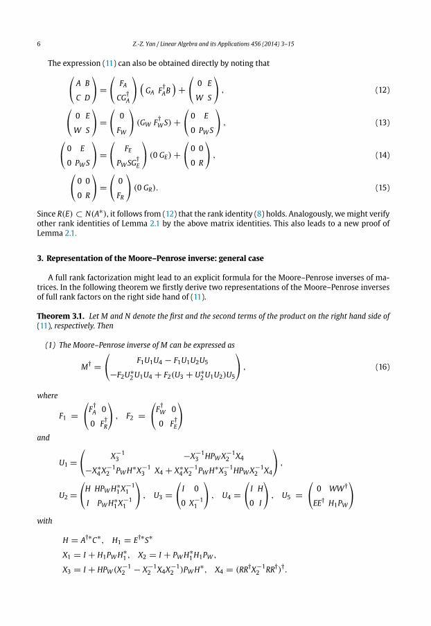
The expression (11) can also be obtained directly by noting that

⎛⎝ A B

C D

⎞⎠ =

⎛⎝ FA

CG†A

⎞⎠ (

GA F†AB

)+

⎛⎝ 0 E

W S

⎞⎠ , (12)

⎛⎝ 0 E

W S

⎞⎠ =

⎛⎝ 0

FW

⎞⎠ (GW F

†WS) +

⎛⎝ 0 E

0 PWS

⎞⎠ , (13)

⎛⎝ 0 E

0 PWS

⎞⎠ =

⎛⎝ FE

PWSG†E

⎞⎠ (0 GE) +

⎛⎝ 0 0

0 R

⎞⎠ , (14)

⎛⎝ 0 0

0 R

⎞⎠ =

⎛⎝ 0

FR

⎞⎠ (0 GR). (15)

Since R(E) ⊂ N(A∗), it follows from (12) that the rank identity (8) holds. Analogously, wemight verify

other rank identities of Lemma 2.1 by the above matrix identities. This also leads to a new proof of

Lemma 2.1.

3. Representation of the Moore–Penrose inverse: general case

A full rank factorization might lead to an explicit formula for the Moore–Penrose inverses of ma-

trices. In the following theorem we firstly derive two representations of the Moore–Penrose inverses

of full rank factors on the right side hand of (11).

Theorem 3.1. Let M and N denote the first and the second terms of the product on the right hand side of

(11), respectively. Then

(1) The Moore–Penrose inverse of M can be expressed as

M† =⎛⎝ F1U1U4 − F1U1U2U5

−F2U∗2U1U4 + F2(U3 + U∗

2U1U2)U5

⎞⎠ , (16)

where

F1 =⎛⎝F

†A 0

0 F†R

⎞⎠ , F2 =

⎛⎝F

†W 0

0 F†E

⎞⎠

and

U1 =⎛⎝ X

−13 −X

−13 HPWX

−12 X4

−X∗4X

−12 PWH∗X−1

3 X4 + X∗4X

−12 PWH∗X−1

3 HPWX−12 X4

⎞⎠ ,

U2 =⎛⎝H HPWH∗

1X−11

I PWH∗1X

−11

⎞⎠ , U3 =

⎛⎝ I 0

0 X−11

⎞⎠ , U4 =

⎛⎝ I H

0 I

⎞⎠ , U5 =

⎛⎝ 0 WW†

EE† H1PW

⎞⎠

with

H = A†∗C∗, H1 = E†∗S∗

X1 = I + H1PWH∗1 , X2 = I + PWH∗

1H1PW ,

X3 = I + HPW (X−12 − X

−12 X4X

−12 )PWH∗, X4 = (RR†X−1

2 RR†)†.


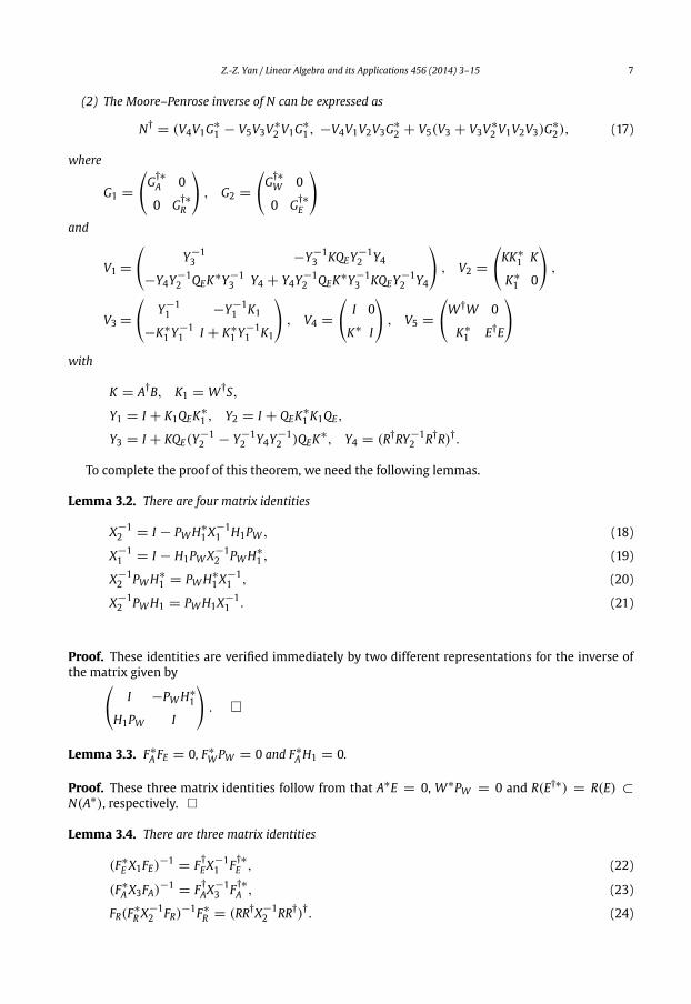
(2) The Moore–Penrose inverse of N can be expressed as

N† = (V4V1G∗1 − V5V3V

∗2 V1G

∗1, −V4V1V2V3G

∗2 + V5(V3 + V3V

∗2 V1V2V3)G

∗2), (17)

where

G1 =⎛⎝G

†∗A 0

0 G†∗R

⎞⎠ , G2 =

⎛⎝G

†∗W 0

0 G†∗E

⎞⎠

and

V1 =⎛⎝ Y

−13 −Y

−13 KQEY

−12 Y4

−Y4Y−12 QEK

∗Y−13 Y4 + Y4Y

−12 QEK

∗Y−13 KQEY

−12 Y4

⎞⎠ , V2 =

⎛⎝KK∗

1 K

K∗1 0

⎞⎠ ,

V3 =⎛⎝ Y

−11 −Y

−11 K1

−K∗1 Y

−11 I + K∗

1 Y−11 K1

⎞⎠ , V4 =

⎛⎝ I 0

K∗ I

⎞⎠ , V5 =

⎛⎝W†W 0

K∗1 E†E

⎞⎠

with

K = A†B, K1 = W†S,

Y1 = I + K1QEK∗1 , Y2 = I + QEK

∗1 K1QE,

Y3 = I + KQE(Y−12 − Y

−12 Y4Y

−12 )QEK

∗, Y4 = (R†RY−12 R†R)†.

To complete the proof of this theorem, we need the following lemmas.

Lemma 3.2. There are four matrix identities

X−12 = I − PWH∗

1X−11 H1PW , (18)

X−11 = I − H1PWX

−12 PWH∗

1 , (19)

X−12 PWH∗

1 = PWH∗1X

−11 , (20)

X−12 PWH1 = PWH1X

−11 . (21)

Proof. These identities are verified immediately by two different representations for the inverse of

the matrix given by⎛⎝ I −PWH∗

1

H1PW I

⎞⎠ . �

Lemma 3.3. F∗A FE = 0, F∗

WPW = 0 and F∗AH1 = 0.

Proof. These three matrix identities follow from that A∗E = 0, W∗PW = 0 and R(E†∗) = R(E) ⊂N(A∗), respectively. �

Lemma 3.4. There are three matrix identities

(F∗E X1FE)

−1 = F†EX

−11 F

†∗E , (22)

(F∗A X3FA)

−1 = F†AX

−13 F

†∗A , (23)

FR(F∗R X

−12 FR)

−1F∗R = (RR†X−1

2 RR†)†. (24)


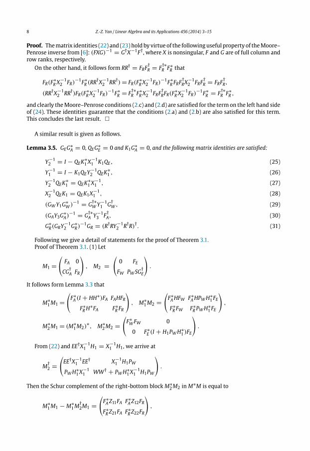
Proof. Thematrix identities (22) and (23) hold by virtue of the followinguseful property of theMoore–

Penrose inverse from [6]: (FXG)−1 = G†X−1F†, where X is nonsingular, F and G are of full column and

row ranks, respectively.

On the other hand, it follows form RR† = FRF†R = F

†∗R F∗

R that

FR(F∗R X

−12 FR)

−1F∗R (RR†X−1

2 RR†) = FR(F∗R X

−12 FR)

−1F∗R FRF

†RX

−12 FRF

†R = FRF

†R,

(RR†X−12 RR†)FR(F

∗R X

−12 FR)

−1F∗R = F

†∗R F∗

R X−12 FRF

†RFR(F

∗R X

−12 FR)

−1F∗R = F

†∗R F∗

R ,

and clearly theMoore–Penrose conditions (2.c) and (2.d) are satisfied for the term on the left hand side

of (24). These identities guarantee that the conditions (2.a) and (2.b) are also satisfied for this term.

This concludes the last result. �

A similar result is given as follows.

Lemma 3.5. GEG∗A = 0, QEG

∗E = 0 and K1G

∗A = 0, and the following matrix identities are satisfied:

Y−12 = I − QEK

∗1 X

−11 K1QE, (25)

Y−11 = I − K1QEY

−12 QEK

∗1 , (26)

Y−12 QEK

∗1 = QEK

∗1 X

−11 , (27)

X−12 QEK1 = QEK1X

−11 , (28)

(GWY1G∗W )−1 = G

†∗WY

−11 G

†W , (29)

(GAY3G∗A)

−1 = G†∗A Y

−13 F

†A, (30)

G∗R(GRY

−12 G∗

R)−1GR = (R†RY−1

2 R†R)†. (31)

Following we give a detail of statements for the proof of Theorem 3.1.

Proof of Theorem 3.1. (1) Let

M1 =⎛⎝ FA 0

CG†A FR

⎞⎠ , M2 =

⎛⎝ 0 FE

FW PWSG†E

⎞⎠ .

It follows form Lemma 3.3 that

M∗1M1 =

⎛⎝F∗

A (I + HH∗)FA FAHFR

F∗R H

∗FA F∗R FR

⎞⎠ , M∗

1M2 =⎛⎝F∗

AHFW F∗AHPWH∗

1FE

F∗R FW F∗

R PWH∗1FE

⎞⎠ ,

M∗2M1 = (M∗

1M2)∗, M∗

2M2 =⎛⎝F∗

WFW 0

0 F∗E (I + H1PWH∗

1 )FE

⎞⎠ .

From (22) and EE†X−11 H1 = X

−11 H1, we arrive at

M†2 =

⎛⎝EE†X

−11 EE† X

−11 H1PW

PWH∗1X

−11 WW† + PWH∗

1X−11 H1PW

⎞⎠ .

Then the Schur complement of the right-bottom block M∗2M2 in M∗M is equal to

M∗1M1 − M∗

1M†2M1 =

⎛⎝F∗

A Z11FA F∗A Z12FR

F∗R Z21FA F∗

R Z22FR

⎞⎠ ,


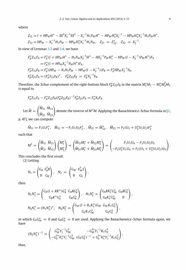
where

Z11 = I + HPWH∗ − EE†X−11 EE† − X

−11 H1PWH∗ − HPWH∗

1X−11 − HPWH∗

1X−11 H1PWH∗,

Z12 = HPW − X−11 H1PW − HPWH∗

1X−11 H1PW , Z21 = Z∗

12, Z22 = X−12 .

In view of Lemmas 3.3 and 3.4, we have

F∗A Z11FA = F∗

A (I + HPWH∗ − H1PWX−12 H∗ − HX

−12 PWH∗

1 − HPW (I − X−12 )PWH∗)FA

= F∗A (I + HPWX

−12 PWH∗)FA,

F∗A Z12FR = F∗

A (HPW − X1H1PW − HPW (I − X−12 ))FR = F∗

AHPWX−12 FR,

F∗R Z21FA = (F∗

A Z12FR)∗, F∗

R Z22FR = F∗R X

−12 FR.

Therefore, the Schur complement of the right-bottom block F∗R Z22FR in the matrix M∗

1M1 − M∗1M

†2M1

is equal to

F∗A Z11FA − F∗

A Z12FR(F∗R Z22FR)

−1F∗R Z21FA = F∗

A X3FA.

Let M =⎛⎝M11 M12

M21 M22

⎞⎠ denote the inverse ofM∗M. Applying the Banachiewicz–Schur formula in [2,

p. 47], we can compute

M11 = F1U1F∗1 , M12 = −F1U1U2F

∗2 , M21 = M∗

12, M22 = F2(U3 + U∗2U1U2)F

∗2

such that

M† =⎛⎝M11 M12

M21 M22

⎞⎠

⎛⎝M∗

1

M∗2

⎞⎠ =

⎛⎝M11M

∗1 + M12M

∗2

M21M∗1 + M22M

∗2

⎞⎠ =

⎛⎝ F1U1U4 − F1U1U2U5

−F2U∗2U1U4 + F2(U3 + U∗

2U1U2)U5

⎞⎠ .

This concludes the first result.

(2) Letting

N1 =⎛⎝GA F

†AB

0 GR

⎞⎠ , N2 =

⎛⎝GW F

†WS

0 GE

⎞⎠ ,

then

N1N∗1 =

⎛⎝GA(I + KK∗)G∗

A GAKG∗R

GRK∗G∗

A GRG∗R

⎞⎠ , N1N

∗2 =

⎛⎝GAKK

∗1G

∗W GAKG

∗E

GRK∗1G

∗W 0

⎞⎠ ,

N2N∗1 = (N1N

∗2 )

∗, N2N∗2 =

⎛⎝GW (I + K1K

∗1 )GW GWK1G

∗E

GEK1G∗W GEG

∗E

⎞⎠ ,

in which GAG∗W = 0 and GRG

∗E = 0 are used. Applying the Banachiewicz–Schur formula again, we

have

(N2N∗2 )

−1 =⎛⎝ G

†∗WY

−11 G

†W −G

†∗WY

−11 K1G

†E

−G†∗E K∗

1 Y−11 G

†W (GEG

∗E )

−1 + G†∗E K∗

1 Y−11 K1G

†E

⎞⎠ ,

thus,


N†2 =

⎛⎝W†WY

−11 W†W Y

−11 K1QE

QEK∗1 Y

−11 E†E + QEK

∗1 Y

−11 K1QE

⎞⎠ .

Let N =⎛⎝N11 N12

N21 N22

⎞⎠ denote the inverse of N. As in the proof of the first part, we arrive at

N1N∗1 − N1N

†2N

∗1 =

⎛⎝GA(I + KQEY

−12 QEK

∗)G∗A GAKQEY

−12 G∗

R

GRY−12 QEK

∗G∗A GRY

−12 G∗

R

⎞⎠

such that

N† = (N∗1 N∗

2 )

⎛⎝N11 N12

N21 N22

⎞⎠ = (N∗

1 N11 + N∗2 N21, N∗

1 N12 + N∗2 N22)

= (V4V1G∗1 + V5V3V

∗2 V1G

∗1, −V4V1V2V3G

∗2 + V5(V3 + V3V

∗2 V1V2V3)G

∗2).

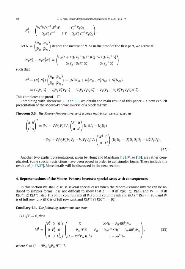
This completes the proof. �Combining with Theorems 2.1 and 3.1, we obtain the main result of this paper – a new explicit

presentation of the Moore–Penrose inverse of a block matrix.

Theorem 3.6. The Moore–Penrose inverse of a block matrix can be expressed as

⎛⎝A B

C D

⎞⎠

†

= (V4 − V5V3V∗2 )V1

⎛⎝A† 0

0 R†

⎞⎠U1(U4 − U2U5)

+(V5 + V5V3V∗2 V1V2 − V4V1V2)V3

⎛⎝W† 0

0 E†

⎞⎠ (U3U5 + U∗

2U1U2U5 − U∗2U1U4).

(32)

Another two explicit presentations, given by Hung and Markham [12], Miao [16], are rather com-

plicated. Some special restrictions have been posed in order to get simpler forms. These include the

results of [4,17,27]. More details will be discussed in the next section.

4. Representations of the Moore–Penrose inverses: special cases with consequences

In this section we shall discuss several special cases when the Moore–Penrose inverse can be re-

duced to simpler forms. It is not difficult to show that E = 0 iff R(B) ⊂ R(A), and W = 0 iff

R(C∗) ⊂ R(A∗); also, E is of full column rank iff B is of full column rank and R(A) ∩ R(B) = {0}, andW

is of full row rank iff C is of full row rank and R(A∗) ∩ R(C∗) = {0}.Corollary 4.1. The following statements are true:

(1) If E = 0, then

M† =

⎛⎜⎜⎜⎝F†A 0 0

0 F†R 0

0 0 F†W

⎞⎟⎟⎟⎠

⎛⎜⎜⎜⎝

X XH(I − PWRR†)PW

−PWH∗X PW − PWH∗XH(I − PWRR†)PW

(I − RR†PW )H∗X I − RR†PW

⎞⎟⎟⎟⎠ , (33)

where X = (I + HPWPRPWH∗)−1.


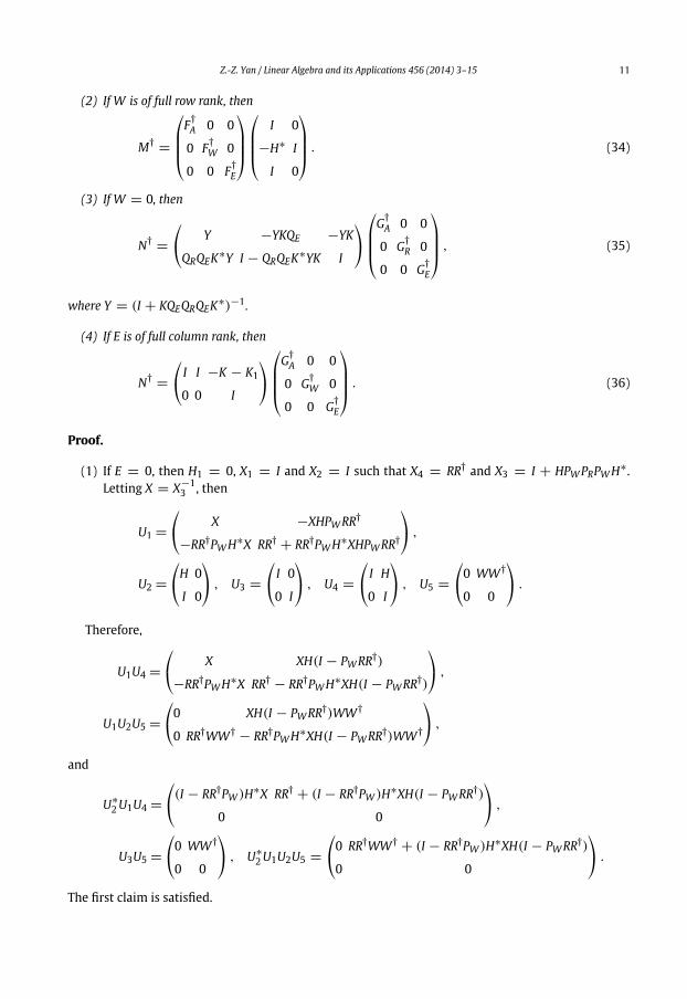
(2) If W is of full row rank, then

M† =

⎛⎜⎜⎜⎝F†A 0 0

0 F†W 0

0 0 F†E

⎞⎟⎟⎟⎠

⎛⎜⎜⎜⎝

I 0

−H∗ I

I 0

⎞⎟⎟⎟⎠ . (34)

(3) If W = 0, then

N† =⎛⎝ Y −YKQE −YK

QRQEK∗Y I − QRQEK

∗YK I

⎞⎠

⎛⎜⎜⎜⎝G†A 0 0

0 G†R 0

0 0 G†E

⎞⎟⎟⎟⎠ , (35)

where Y = (I + KQEQRQEK∗)−1.

(4) If E is of full column rank, then

N† =⎛⎝ I I −K − K1

0 0 I

⎞⎠

⎛⎜⎜⎜⎝G†A 0 0

0 G†W 0

0 0 G†E

⎞⎟⎟⎟⎠ . (36)

Proof.

(1) If E = 0, then H1 = 0, X1 = I and X2 = I such that X4 = RR† and X3 = I + HPWPRPWH∗.Letting X = X

−13 , then

U1 =⎛⎝ X −XHPWRR†

−RR†PWH∗X RR† + RR†PWH∗XHPWRR†

⎞⎠ ,

U2 =⎛⎝H 0

I 0

⎞⎠ , U3 =

⎛⎝ I 0

0 I

⎞⎠ , U4 =

⎛⎝ I H

0 I

⎞⎠ , U5 =

⎛⎝0 WW†

0 0

⎞⎠ .

Therefore,

U1U4 =⎛⎝ X XH(I − PWRR†)

−RR†PWH∗X RR† − RR†PWH∗XH(I − PWRR†)

⎞⎠ ,

U1U2U5 =⎛⎝0 XH(I − PWRR†)WW†

0 RR†WW† − RR†PWH∗XH(I − PWRR†)WW†

⎞⎠ ,

and

U∗2U1U4 =

⎛⎝(I − RR†PW )H∗X RR† + (I − RR†PW )H∗XH(I − PWRR†)

0 0

⎞⎠ ,

U3U5 =⎛⎝0 WW†

0 0

⎞⎠ , U∗

2U1U2U5 =⎛⎝0 RR†WW† + (I − RR†PW )H∗XH(I − PWRR†)

0 0

⎞⎠ .

The first claim is satisfied.


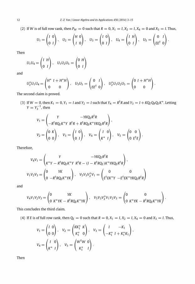
(2) IfW is of full row rank, then PW = 0 such that R = 0, X1 = I, X2 = I, X4 = 0 and X3 = I. Thus,

U1 =⎛⎝ I 0

0 I

⎞⎠ , U2 =

⎛⎝H 0

I 0

⎞⎠ , U3 =

⎛⎝ I 0

0 I

⎞⎠ , U4 =

⎛⎝ I H

0 I

⎞⎠ , U5 =

⎛⎝ 0 I

EE† 0

⎞⎠ .

Then

U1U4 =⎛⎝ I H

0 I

⎞⎠ , U1U2U5 =

⎛⎝0 H

0 I

⎞⎠

and

U∗2U1U4 =

⎛⎝H∗ I + H∗H

0 0

⎞⎠ , U3U5 =

⎛⎝ 0 I

EE† 0

⎞⎠ , U∗

2U1U2U5 =⎛⎝0 I + H∗H0 0

⎞⎠ .

The second claim is proved.

(3) IfW = 0, then K1 = 0, Y1 = I and Y2 = I such that Y4 = R†R and Y3 = I +KQEQRQEK∗. Letting

Y = Y−13 , then

V1 =⎛⎝ Y −YKQER

†R

−R†RQEK∗Y R†R + R†RQEK

∗YKQER†R

⎞⎠ ,

V2 =⎛⎝0 K

0 0

⎞⎠ , V3 =

⎛⎝ I 0

0 I

⎞⎠ , V4 =

⎛⎝ I 0

K∗ I

⎞⎠ , V5 =

⎛⎝0 0

0 E†E

⎞⎠ .

Therefore,

V4V1 =⎛⎝ Y −YKQER

†R

K∗Y − R†RQEK∗Y R†R − (I − R†RQE)K

∗YKQER†R

⎞⎠ ,

V1V2V3 =⎛⎝0 YK

0 −R†RQEK∗YK

⎞⎠ , V5V3V

∗2 V1 =

⎛⎝ 0 0

E†EK∗Y −E†EK∗YKQER†R

⎞⎠

and

V4V1V2V3 =⎛⎝0 YK

0 K∗YK − R†RQEK∗YK

⎞⎠ , V5V3V

∗2 V1V2V3 =

⎛⎝0 0

0 K∗YK − R†RQEK∗YK

⎞⎠ .

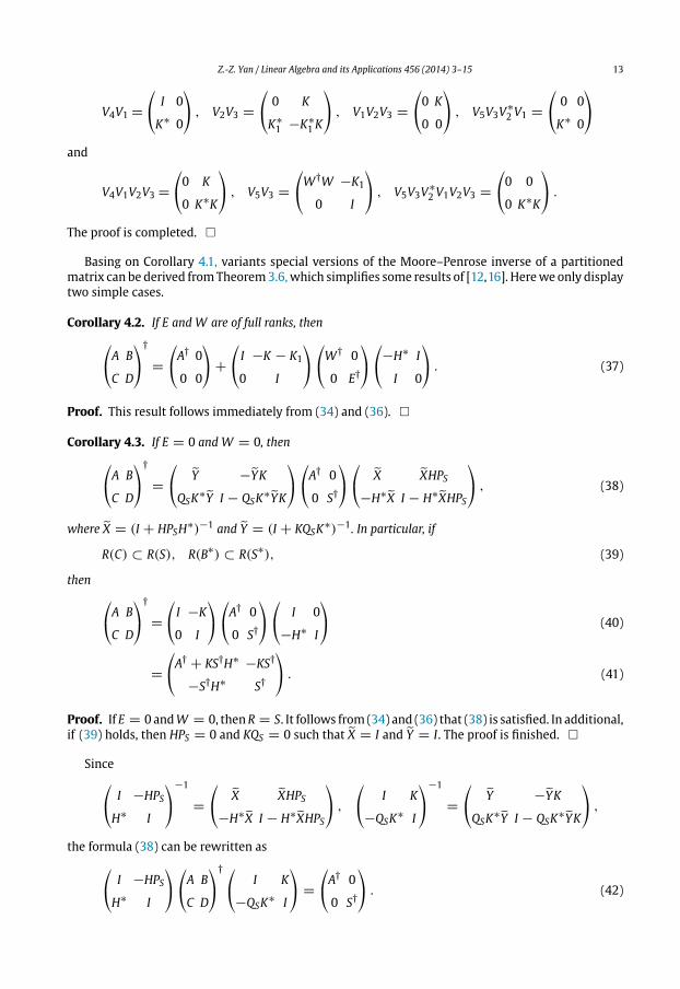
This concludes the third claim.

(4) If E is of full row rank, then QE = 0 such that R = 0, X1 = I, X2 = I, X4 = 0 and X3 = I. Thus,

V1 =⎛⎝ I 0

0 0

⎞⎠ , V2 =

⎛⎝KK∗

1 K

K∗1 0

⎞⎠ , V3 =

⎛⎝ I −K1

−K∗1 I + K∗

1 K1

⎞⎠ ,

V4 =⎛⎝ I 0

K∗ I

⎞⎠ , V5 =

⎛⎝W†W 0

K∗1 I

⎞⎠ .

Then


V4V1 =⎛⎝ I 0

K∗ 0

⎞⎠ , V2V3 =

⎛⎝ 0 K

K∗1 −K∗

1 K

⎞⎠ , V1V2V3 =

⎛⎝0 K

0 0

⎞⎠ , V5V3V

∗2 V1 =

⎛⎝ 0 0

K∗ 0

⎞⎠

and

V4V1V2V3 =⎛⎝0 K

0 K∗K

⎞⎠ , V5V3 =

⎛⎝W†W −K1

0 I

⎞⎠ , V5V3V

∗2 V1V2V3 =

⎛⎝0 0

0 K∗K

⎞⎠ .

The proof is completed. �

Basing on Corollary 4.1, variants special versions of the Moore–Penrose inverse of a partitioned

matrix can be derived fromTheorem3.6,which simplifies some results of [12,16]. Herewe only display

two simple cases.

Corollary 4.2. If E and W are of full ranks, then

⎛⎝A B

C D

⎞⎠

†

=⎛⎝A† 0

0 0

⎞⎠ +

⎛⎝ I −K − K1

0 I

⎞⎠

⎛⎝W† 0

0 E†

⎞⎠

⎛⎝−H∗ I

I 0

⎞⎠ . (37)

Proof. This result follows immediately from (34) and (36). �

Corollary 4.3. If E = 0 and W = 0, then

⎛⎝A B

C D

⎞⎠

†

=⎛⎝ Y −YK

QSK∗Y I − QSK

∗YK

⎞⎠

⎛⎝A† 0

0 S†

⎞⎠

⎛⎝ X XHPS

−H∗X I − H∗XHPS

⎞⎠ , (38)

where X = (I + HPSH∗)−1 and Y = (I + KQSK

∗)−1. In particular, if

R(C) ⊂ R(S), R(B∗) ⊂ R(S∗), (39)

then

⎛⎝A B

C D

⎞⎠

†

=⎛⎝ I −K

0 I

⎞⎠

⎛⎝A† 0

0 S†

⎞⎠

⎛⎝ I 0

−H∗ I

⎞⎠ (40)

=⎛⎝A† + KS†H∗ −KS†

−S†H∗ S†

⎞⎠ . (41)

Proof. If E = 0 andW = 0, thenR = S. It follows from (34) and (36) that (38) is satisfied. In additional,

if (39) holds, then HPS = 0 and KQS = 0 such that X = I and Y = I. The proof is finished. �

Since

⎛⎝ I −HPS

H∗ I

⎞⎠

−1

=⎛⎝ X XHPS

−H∗X I − H∗XHPS

⎞⎠ ,

⎛⎝ I K

−QSK∗ I

⎞⎠

−1

=⎛⎝ Y −YK

QSK∗Y I − QSK

∗YK

⎞⎠ ,

the formula (38) can be rewritten as

⎛⎝ I −HPS

H∗ I

⎞⎠

⎛⎝A B

C D

⎞⎠

† ⎛⎝ I K

−QSK∗ I

⎞⎠ =

⎛⎝A† 0

0 S†

⎞⎠ . (42)


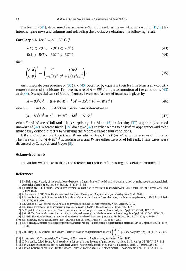
The formula (41), also named Banachiewicz–Schur formula, is the well-known result of [11,12]. By

interchanging rows and columns and relabeling the blocks, we obtained the following result.

Corollary 4.4. Let T = A − BD†C. If

R(C) ⊂ R(D), R(B∗) ⊂ R(D∗), (43)

R(B) ⊂ R(T), R(C∗) ⊂ R(T∗), (44)

then

⎛⎝A B

C D

⎞⎠

†

=⎛⎝ T† −T†BA†

−D†CT† D† + D†CT†BD†

⎞⎠ . (45)

An immediate consequence of (32) and (45) obtained by equating their leading term is an explicitly

representation of the Moore–Penrose inverse of A − BD†C on the assumption of the conditions (43)

and (44). One special case of Moore–Penrose inverses of a sum of matrices is given by

(A − BD†C)† = (I + KQSK∗)−1(A† + KS†H∗)(I + HPSH

∗)−1 (46)

when E = 0 and W = 0. Another special case is described as

(A − BD†C)† = A† − W†H∗ − KE† − W†SE† (47)

when E and W are of full ranks. It is surprising that Miao [16], in deriving (37), apparently seemed

unaware of (47), whereas Riedel [25] does give (47), in what seems to be its first appearance and to be

more easily derived directly by verifying the Moore–Penrose four conditions.

If B and C are vectors, then E and W are also vectors; thus E (or W) is either zero or of full rank.

Then we can find (A + bc∗)† according as E and W are either zero or of full rank. These cases were

discussed by Campbell and Meyer [5].

Acknowledgments

The author would like to thank the referees for their careful reading and detailed comments.

References

[1] J.K. Baksalary, A study of the equivalence between a Gauss–Markoff model and its augmentation by nuisance parameters, Math.Operationsforsch. u. Statist., Ser. Statist. 15 (1984) 3–35.

[2] J.K. Baksalary, G.P.H. Styan, Generalized inverses of partitioned matrices in Banachiewicz–Schur form, Linear Algebra Appl. 354(2002) 41–47.

[3] A. Ben-Israel, T.N.E. Greville, Generalized Inverses: Theory and Applications, John Wiley, New York, 1974.[4] F. Burns, D. Carlson, E. Haynsworth, T. Markham, Generalized inverse formulas using the Schur-complement, SIAM J. Appl. Math.

26 (1974) 254–259.

[5] S.L. Campbell, C.D. Meyer Jr., Generalized Inverses of Linear Transformations, Pitan, London, 1979.[6] R.E. Cline, Inverses of rank invariant powers of a matrix, SIAM J. Numer. Anal. 5 (1968) 182–197.

[7] A. Cegielski, Obtuse cones and Gram matrices with non-negative inverse, Linear Algebra Appl. 335 (2001) 167–181.[8] J. Groß, The Moore–Penrose inverse of a partitioned nonnegative definite matrix, Linear Algebra Appl. 321 (2000) 113–121.

[9] F.J. Hall, The Moore–Penrose inverse of particular bordered matrices, J. Austral. Math. Soc., Ser. A 27 (1979) 467–478.[10] R.E. Hartwig, Block generalized inverses, Arch. Ration. Mech. Anal. 61 (1976) 197–251.

[11] R.E. Hartwig, Singular value decomposition and the Moore–Penrose inverse of bordered matrices, SIAM J. Appl. Math. 31 (1976)

31–41.

[12] C.H. Hung, T.L. Markham, The Moore–Penrose inverse of a partitioned matrix

⎛⎝ A D

B C

⎞⎠, Linear Algebra Appl. 11 (1975) 73–86.

[13] P. Lancaster, M. Tismenetsky, The Theory of Matrices with Applications, Academic Press, 1985.[14] G. Marsaglia, G.P.H. Styan, Rank conditions for generalized inverse of partitioned matrices, Sankhya Ser. 36 (1974) 437–442.

[15] J. Miao, Representations for the weighted Moore–Penrose of a partitioned matrix, J. Comput. Math. 7 (1989) 320–323.[16] J. Miao, General expressions for the Moore–Penrose inverse of a 2 × 2 block matrix, Linear Algebra Appl. 151 (1991) 1–15.


[17] D.C. Meyer Jr., Generalized inverses and ranks of block matrices, SIAM J. Appl. Math. 25 (1973) 597–602.

[18] G.V. Milovanovic, P.S. Stanimirovic, On Moore–Penrose inverse of block matrices and full rank factorizations, Publ. Inst. Math.62 (1997) 26–40.

[19] E.H. Moore, On the reciprocal of the general algebraic matrix, Bull. Amer. Math. Soc. 26 (1920) 394–395.[20] B. Noble, A method for computing the generalized inverse of a matrix, SIAM J. Numer. Anal. 3 (1966) 582–584.

[21] B. Noble, Applied Linear Algebra, Prentice-Hall, New Jersey, 1969.

[22] R. Penrose, A generalized inverse for matrices, Proc. Cambridge Philos. Soc. 51 (1955) 406–413.[23] R. Piziak, P.L. OdellSource, Full rank factorization of matrices, Math. Mag. 72 (1999) 193–201.

[24] R.M. Pringle, A.A. Rayner, Expressions for generalized inverses of a borderedmatrixwith application to the theory of constrainedlinear models, SIAM Rev. 12 (1970) 107–115.

[25] K. Riedel, A Sherman–Morrison–Woodbury identity for rank augmentingmatrices with application to centering, SIAM J. MatrixAnal. Appl. 13 (1992) 659–662.

[26] J.V. Rao, S.K. Mitra, Generalized Inverse of Matrices and its Applications, John Wiley, New York, 1971.[27] C.A. Rohde, Generalized inverses of partitioned matrices, SIAM J. Appl. Math. 13 (1965) 1033–1035.

[28] P. Robert, On the group inverse of a linear transformation, J. Math. Appl. 22 (1968) 658–699.

[29] R.P. Tewarson, A direct method for generalized matrix inversion, SIAM J. Numer. Anal. 4 (1967) 499–507.[30] Y. Tian, Y. Takane, More on generalized inverses of partitioned matrices with Banachiewicz–Schur forms, Linear Algebra Appl.

430 (2009) 1641–1655.

[31] G. Wang, Y. Chen, A recursive algorithm for computing the weighted Moore–Penrose inverse A†M,N , J. Comput. Math. 4 (1986)

74–85.[32] S. Zlobec, An explicit form the Moore–Penrose inverse of an arbitrary complex matrix, SIAM Rev. 12 (1970) 132–134.


Reshetov LA New representations of the Moore–Penrose inverse of 2 × 2 block matrices

Documents

Transcript of Reshetov LA New representations of the Moore–Penrose inverse of 2 × 2 block matrices