Available online at www.sciencedirect.com

ScienceDirect

Journal of Approximation Theory 185 (2014) 63–79www.elsevier.com/locate/jat

Full length article

The rate of linear convergence of the Douglas–Rachfordalgorithm for subspaces is the cosine of the

Friedrichs angle

Heinz H. Bauschkea,∗, J.Y. Bello Cruzb, Tran T.A. Nghiaa,Hung M. Phana, Xianfu Wanga

a Mathematics, University of British Columbia, Kelowna, B.C. V1V 1V7, Canadab IME, Federal University of Goias, Goiania, G.O. 74001-970, Brazil

Received 15 February 2014; received in revised form 24 April 2014; accepted 6 June 2014Available online 19 June 2014

Communicated by Patrick Combettes

Abstract

The Douglas–Rachford splitting algorithm is a classical optimization method that has found manyapplications. When specialized to two normal cone operators, it yields an algorithm for finding a pointin the intersection of two convex sets. This method for solving feasibility problems has attracted a lot ofattention due to its good performance even in nonconvex settings.

In this paper, we consider the Douglas–Rachford algorithm for finding a point in the intersection oftwo subspaces. We prove that the method converges strongly to the projection of the starting point onto theintersection. Moreover, if the sum of the two subspaces is closed, then the convergence is linear with the ratebeing the cosine of the Friedrichs angle between the subspaces. Our results improve upon existing resultsin three ways: First, we identify the location of the limit and thus reveal the method as a best approximationalgorithm; second, we quantify the rate of convergence, and third, we carry out our analysis in general(possibly infinite-dimensional) Hilbert space. We also provide various examples as well as a comparisonwith the classical method of alternating projections.

∗ Corresponding author.E-mail addresses: heinz.bauschke@ubc.ca (H.H. Bauschke), yunier.bello@gmail.com (J.Y. Bello Cruz),

nghia.tran@ubc.ca (T.T.A. Nghia), hung.phan@ubc.ca (H.M. Phan), shawn.wang@ubc.ca (X. Wang).

http://dx.doi.org/10.1016/j.jat.2014.06.0020021-9045/ c⃝ 2014 Elsevier Inc. All rights reserved.

64 H.H. Bauschke et al. / Journal of Approximation Theory 185 (2014) 63–79

c⃝ 2014 Elsevier Inc. All rights reserved.

MSC: primary 49M27; 65K05; 65K10; secondary 47H05; 47H09; 49M37; 90C25

Keywords: Douglas–Rachford splitting method; Firmly nonexpansive; Friedrichs angle; Linear convergence; Method ofalternating projections; Normal cone operator; Subspaces; Projection operator

1. Introduction

Throughout this paper, we assume that

X is a real Hilbert space (1)

with inner product ⟨·, ·⟩ and induced norm ∥ · ∥. Let U and V be closed convex subsets of Xsuch that U ∩ V = ∅. The convex feasibility problem is to find a point in U ∩ V . This is a basicproblem in the natural sciences and engineering (see, e.g., [5,15], and [16]) — as such, a plethoraof algorithms based on the nearest point mappings (projectors) PU and PV have been proposedto solve it.

One particularly popular method is the Douglas–Rachford splitting algorithm [22] whichutilizes the Douglas–Rachford splitting operator1

T := PV (2PU − Id) + Id −PU (2)

and x0 ∈ X to generate the sequence (xn)n∈N by

(∀n ∈ N) xn+1 := T xn . (3)

While the sequence (xn)n∈N may or may not converge to a point in U ∩ V , the projected(“shadow”) sequence

(PU xn)n∈N (4)

always converges (weakly) to a point in U ∩ V (see [30,17,32,4,7]). The Douglas–Rachfordalgorithm has been applied very successfully to various problems where U and V are notnecessarily convex, even though the supporting formal theory is far from being complete (see,e.g., [1,8], and [24]). Very recently, Hesse, Luke and Neumann [27] (see also [26]) consideredprojection methods for the (nonconvex) sparse affine feasibility problem. Their paper highlightsthe importance of understanding the Douglas–Rachford algorithm for the case when U and Vare closed subspaces2 of X ; their basic convergence result is the following.

Fact 1.1 (Hesse–Luke–Neumann). (See [27, Theorem 4.6].) Suppose that X is finite-dimensionaland U and V are subspaces of X. Then the sequence (xn)n∈N generated by (3) converges to apoint in Fix T := {x ∈ X | x = T x} with a linear rate.3

1 Throughout this paper, we write α := β to indicate that α is defined to be equal to β.2 Throughout this paper, we use the term “subspace” to denote a (not necessarily closed) vector subspace in the sense

of Linear Algebra.3 Recall that xn → x linearly or with a linear rate γ ∈ ]0, 1[ if (γ −n

∥xn − x∥)n∈N is bounded.

H.H. Bauschke et al. / Journal of Approximation Theory 185 (2014) 63–79 65

The aim of this paper is three-fold. We complement Fact 1.1 by providing the following:

• We identify the limit of the shadow sequence (PU xn)n∈N as PU∩V x0; consequently andsomewhat surprisingly, the Douglas–Rachford method in this setting not only solves afeasibility problem but actually a best approximation problem.

• We quantify the rate of convergence—it turns out to be the cosine of the Friedrichs anglebetween U and V ; moreover, our estimate is sharp.

• Our analysis is carried out in general (possibly infinite-dimensional) Hilbert space.

The paper is organized as follows. In Sections 2 and 3, we collect various auxiliary resultsto facilitate the proof of the main results (Theorems 4.1 and 4.3) in Section 4. In Section 5,we analyze the Douglas–Rachford algorithm for two lines in the Euclidean plane. The resultsobtained are used in Section 6 for an infinite-dimensional construction illustrating the lack oflinear convergence. In Section 7, we compare the Douglas–Rachford algorithm to the method ofalternating projections. We report on numerical experiments in Section 8, and conclude the paperin Section 9.

Notation is standard and follows largely [7]. We write U ⊕ V to indicate that the terms of theMinkowski sum U + V = {u + v | u ∈ U, v ∈ V } satisfy U ⊥ V .

2. Auxiliary results

In this section, we collect various results to ease the derivation of the main results.

2.1. Firmly nonexpansive mappings

It is well known (see [30,23], or [8]) that the Douglas–Rachford operator T (see (2)) is firmlynonexpansive, i.e.,

(∀x ∈ X)(∀y ∈ X) ∥T x − T y∥2+ ∥(Id −T )x − (Id −T )y∥

2≤ ∥x − y∥

2. (5)

The following result will be useful in our analysis.

Fact 2.1. (See [7, Corollary 5.16 and Proposition 5.27], or [11, Theorem 2.2], [3] and [14].) LetT : X → X be linear and firmly nonexpansive, and let x ∈ X. Then T n x → PFix T x.

2.2. Products of projections and the Friedrichs angle

Unless otherwise stated, we assume from now on that

U and V are closed subspaces of X . (6)

The proof of the following useful fact can be found in [21, Lemma 9.2]:

U ⊆ V ⇒ PU (V ) ⊆ V ⇔ PV PU = PU PV = PU∩V . (7)

Our main results are formulated using the notion of the Friedrichs angle between U and V .Let us review the definition and provide the key results which are needed in the sequel.

Definition 2.2. The cosine of the Friedrichs angle between U and V is

cF := sup|⟨u, v⟩| | u ∈ U ∩ (U ∩ V )⊥, v ∈ V ∩ (U ∩ V )⊥, ∥u∥ ≤ 1, ∥v∥ ≤ 1

. (8)

We write cF (U, V ) for cF if we emphasize the subspaces utilized.

66 H.H. Bauschke et al. / Journal of Approximation Theory 185 (2014) 63–79

Fact 2.3 (Fundamental Properties of the Friedrichs Angle). Let n ∈ {1, 2, 3, . . .}. Then thefollowing hold:

(i) U + V is closed ⇔ cF < 1.(ii) cF (U, V ) = cF (V, U ) = cF (U⊥, V ⊥).

(iii) cF = ∥PV PU − PU∩V ∥ = ∥PV ⊥ PU⊥ − PU⊥∩V ⊥∥.(iv) (Aronszajn–Kayalar–Weinert) ∥(PV PU )n

− PU∩V ∥ = c2n−1F .

Proof. (i): See [20, Theorem 13] (ii): See [20, Theorem 16] (iii): See [21, Lemma 9.5(7)] and(ii) above. (iv): See [21, Theorem 9.31] (or the original works [2] and [29]). �

Note that Fact 2.3(ii)&(iii) yield

cF = 0 ⇔ PV PU = PU PV = PU∩V . (9)

The classical Fact 2.3(iv) deals with even powers of alternating projectors. We complementthis result by deriving the counterpart for odd powers.

Lemma 2.4 (Odd Powers of Alternating Projections). Let n ∈ {1, 2, 3, . . .}. Then

∥PU (PV PU )n− PU∩V ∥ = c2n

F . (10)

Proof. If cF = 0, then the conclusion is clear from (9). We thus assume that cF > 0. By (7),(PU PV )n

− PU∩V

PV PU − PU∩V

= (PU PV )n PV PU − (PU PV )n PU∩V − PU∩V PV PU + P2U∩V (11a)

= (PU PV )n PU − PU∩V − PU∩V + PU∩V (11b)

= PU (PV PU )n− PU∩V . (11c)

It thus follows from Fact 2.3(iv)&(iii) that

∥PU (PV PU )n− PU∩V ∥ ≤ ∥(PU PV )n

− PU∩V ∥ · ∥PV PU − PU∩V ∥ = c2nF . (12)

Since (PU (PV PU )n− PU∩V )(PU PV − PU∩V ) = (PU PV )n+1

− PU∩V , we obtain fromFact 2.3(iv)&(iii) that

c2n+1F = ∥(PU PV )n+1

− PU∩V ∥ ≤ ∥PU (PV PU )n− PU∩V ∥ · ∥PU PV − PU∩V ∥ (13a)

= ∥PU (PV PU )n− PU∩V ∥cF . (13b)

Since cF > 0, we obtain c2nF ≤ ∥PU (PV PU )n

− PU∩V ∥. Combining with (12), we deduce(10). �

3. Basic properties of the Douglas–Rachford splitting operator

We recall that the Douglas–Rachford operator is defined by

T = TV,U := PV (2PU − Id) + Id −PU . (14)

For future reference, we record the following consequence of Fact 2.1.

Corollary 3.1. Let x ∈ X. Then T n x → PFix T x.

H.H. Bauschke et al. / Journal of Approximation Theory 185 (2014) 63–79 67

It will be very useful to work with reflectors, which we define next.

Definition 3.2 (Reflector). The reflector associated with U is

RU := 2PU − Id = PU − PU⊥ . (15)

The following simple yet useful result is easily verified.

Proposition 3.3. The reflector RU is a surjective isometry with

R∗

U = R−1U = −RU⊥ = RU . (16)

We now record several reformulations of T and T ∗ which we will use repeatedly in the paperwithout explicitly mentioning it. Item (i) also appears in [19, Section 2.3]; it is interesting toobserve that the operator T also occurs in the convergence analysis of the Douglas–Rachfordalgorithm applied to ℓ1 minimization with linear constraints.

Proposition 3.4. The following hold:

(i) T =12 Id +

12 RV RU = PV RU + Id −PU = PV PU + PV ⊥ PU⊥ .

(ii) T ∗= PU PV + PU⊥ PV ⊥ = TU,V = T ∗

V,U .(iii) TV,U = TV ⊥,U⊥ .

Proof. (i): Expand and use the linearity of PU and PV . (ii) and (iii): This follows from (i). �

The next result highlights the importance of the reflectors when traversing between T and T ∗.Item (iv) was observed previously in [13, Remark 4.1].

Proposition 3.5. The following hold:

(i) RU T ∗= T RU = T ∗ RV = RV T = PU + PV − Id.

(ii) T ∗(RV RU ) = (RV RU )T ∗= T and T (RU RV ) = (RU RV )T = T ∗.

(iii) T T ∗= T ∗T , i.e., T is normal.

(iv) 2T T ∗= T + T ∗.

(v) T T ∗ is firmly nonexpansive and self-adjoint.(vi) T T ∗

= PV PU PV + PV ⊥ PU⊥ PV ⊥ = PV PU + PU PV − PU − PV + Id = PU PV PU +

PU⊥ PV ⊥ PU⊥ .

Proof. (i): Indeed, using Propositions 3.4(i) and (ii), we see that

T RU = (PV PU + PV ⊥ PU⊥)(PU − PU⊥) = PV PU − PV ⊥ PU⊥

= PV PU − (Id −PV )(Id −PU ) (17a)

= PU + PV − Id (17b)

= PU PV − (Id −PU )(Id −PV ) = PU PV − PU⊥ PV ⊥

= (PU PV + PU⊥ PV ⊥)(PV − PV ⊥) (17c)

= T ∗ RV . (17d)

Because PU + PV − Id is self-adjoint, so are T RU and T ∗ RV . Hence RU T ∗= (T RU )∗ =

T RU = T ∗ RV = (RV T )∗ = RV T by Proposition 3.3.(ii): Clear from (i).(iii): Using (ii), we obtain T T ∗

= T ∗(RV RU )(RU RV )T = T ∗T .

68 H.H. Bauschke et al. / Journal of Approximation Theory 185 (2014) 63–79

(iv): 4T T ∗= (Id +RV RU )(Id +RU RV ) = 2 Id +RV RU + RU RV = 2((Id +RV RU )/2 +

(Id +RU RV )/2) = 2(T + T ∗).(v): Since T and T ∗ are firmly nonexpansive, so is their convex combination (T + T ∗)/2,

which equals T T ∗ by (iv). It is clear that T T ∗ is self-adjoint.(vi): It follows from Proposition 3.4(i)&(ii) that T T ∗

= (PV PU + PV ⊥ PU⊥)(PU PV +

PU⊥ PV ⊥) = PV PU PV + PV ⊥ PU⊥ PV ⊥ , which yields the first equality. Replacing PU⊥ andPV ⊥ by Id −PU and Id −PV , respectively, followed by expanding and simplifying results in thesecond equality. The last equality is proved analogously. �

Parts of our next result were also obtained in [26] and [27] when X is finite-dimensional.Concerning item (ii), we note in passing that if U + V = X , then (U⊥, V ⊥) satisfies the inversebest approximation property; see [18, Corollary 2.12] for details.

Proposition 3.6. Let n ∈ N. Then the following hold:

(i) Fix T = Fix T ∗= Fix T ∗T = (U ∩ V ) ⊕ (U⊥

∩ V ⊥).(ii) Fix T = U ∩ V ⇔ U + V = X.

(iii) PFix T = PU∩V + PU⊥∩V ⊥ .(iv) PFix T T = T PFix T = PFix T .(v) PU PFix T = PV PFix T = PU∩V PFix T = PU∩V = PU∩V PFix T T n

= PU∩V T n .

Proof. (i): Set A = NU and B = NV , where NU denotes the normal cone operator definedby NU (x) =

x∗

∈ X | supu∈U ⟨x∗, u − x⟩ ≤ 0

if x ∈ U and NU (x) = ∅ otherwise.Then (A + B)−1(0) = U ∩ V . Combining [6, Example 2.7 and Corollary 5.5(iii)] yieldsFix T = (U ∩ V ) ⊕ (U⊥

∩ V ⊥). By [11, Lemma 2.1], we have Fix T = Fix T ∗. Since Tand T ∗ are firmly nonexpansive, and 0 ∈ Fix T ∩ Fix T ∗, we apply [7, Corollaries 4.3 and 4.37]to deduce that Fix T ∗T = Fix T ∩ Fix T ∗.

(ii): Using (i), we obtain Fix T = U ∩ V ⇔ U⊥∩ V ⊥

= {0} ⇔ U + V = U⊥⊥ + V ⊥⊥ =

(U⊥∩ V ⊥)⊥ = {0}

⊥= X .

(iii): This follows from (i).(iv): Clearly, T PFix T = PFix T . Furthermore, PFix T T = T PFix T by [11, Lemma 3.12].(v): First, (iii) and (7) imply PU PFix T = PV PFix T = PU∩V PFix T = PU∩V . This and (iv)

give the remaining equalities. �

4. Main result

We now are ready for our main results concerning the dynamical behavior of the Douglas–Rachford iteration.

Theorem 4.1 (Powers of T ). Let n ∈ {1, 2, 3, . . .}, and let x ∈ X. Then

∥T n− PFix T ∥ = cn

F , (18a)

∥(T T ∗)n− PFix T ∥ = c2n

F , (18b)

and

∥T n x − PFix T x∥ ≤ cnF∥x − PFix T x∥ ≤ cn

F∥x∥. (19)

Proof. Set

c := ∥T − PFix T ∥ = ∥T P(Fix T )⊥∥, (20)

H.H. Bauschke et al. / Journal of Approximation Theory 185 (2014) 63–79 69

and observe that the second equality is justified since PFix T = T PFix T . Since T is (firmly)nonexpansive and normal (see Proposition 3.5(iii)), it follows from [11, Lemma 3.15(i)] that

∥T n− PFix T ∥ = cn . (21)

Propositions 3.4(i), 3.6(iii), and (7) imply

(T − PFix T )x =PV PU + PV ⊥ PU⊥

x −

PU∩V + PU⊥∩V ⊥

x (22a)

=PV PU − PU∩V

x

∈V

+PV ⊥ PU⊥ − PU⊥∩V ⊥

x

∈V ⊥

(22b)

=PV PU PU x − PU∩V PU x

+

PV ⊥ PU⊥ PU⊥ x − PU⊥∩V ⊥ PU⊥ x

(22c)

=PV PU − PU∩V

PU x

∈V

+PV ⊥ PU⊥ − PU⊥∩V ⊥

PU⊥ x

∈V ⊥

. (22d)

Hence, using (22d) and Fact 2.3(iii), we obtain

∥(T − PFix T )x∥2

=

PV PU − PU∩VPU x

2+

PV ⊥ PU⊥ − PU⊥∩V ⊥

PU⊥ x

2 (23a)

≤ ∥PV PU − PU∩V ∥2∥PU x∥

2

+PV ⊥ PU⊥ − PU⊥∩V ⊥

2∥PU⊥ x∥

2 (23b)

= c2F∥PU x∥

2+ c2

F∥PU⊥ x∥2 (23c)

= c2F∥x∥

2. (23d)

We deduce that

c = ∥T − PFix T ∥ ≤ cF . (24)

Furthermore, (22b) implies

∥(T − PFix T )x∥2

=

PV PU − PU∩Vx2

+

PV ⊥ PU⊥ − PU⊥∩V ⊥

x2 (25a)

≥

PV PU − PU∩Vx2

. (25b)

This and Fact 2.3(iii) yield

c = ∥T − PFix T ∥ ≥ ∥PV PU − PU∩V ∥ = cF . (26)

Combining (24) and (26), we obtain c = cF . Consequently, (21) yields (18a) while (18b) followsfrom [11, Lemma 3.15.(2)].

Finally, [11, Lemma 3.14(1)&(3)] results in ∥T n x − PFix T x∥ ≤ cn∥x − PFix T x∥ =

cnF∥x − PFix T x∥ = cn

F∥PFix T ⊥ x∥ ≤ cnF∥x∥. �

The following result yields further insights in various powers of T and T ∗.

Proposition 4.2. Let n ∈ N. Then the following hold:

(i) (T T ∗)n= (T ∗T )n

= (PU PV PU )n+ (PU⊥ PV ⊥ PU⊥)n

= (PV PU PV )n+ (PV ⊥ PU⊥ PV ⊥)n

if n ≥ 1.(ii) PU (T T ∗)n

= (PU PV )n PU = (T T ∗)n PU and PV (T T ∗)n= (PV PU )n PV = (PV PU )n PV .

(iii) T 2n= (T T ∗)n(RV RU )n .

70 H.H. Bauschke et al. / Journal of Approximation Theory 185 (2014) 63–79

(iv) T 2n+1= (T T ∗)nT (RV RU )n

= (T T ∗)nT ∗(RV RU )n+1.(v) T 2n

=(PU PV )n PU + (PU⊥ PV ⊥)n PU⊥

(RV RU )n

=(PV PU )n PV + (PV ⊥ PU⊥)n PV ⊥

(RV RU )n .

(vi) T 2n+1=

(PU PV )n+1

+ (PU⊥ PV ⊥)n+1(RV RU )n+1

=(PV PU )n+1

+ (PV ⊥ PU⊥)n+1

(RV RU )n .

Proof. (i): Proposition 3.5(iii)&(vi) yield

(T T ∗)n= (PU PV PU + PU⊥ PV ⊥ PU⊥)n

= (PU PV PU )n+ (PU⊥ PV ⊥ PU⊥)n

; (27)

the last equality follows similarly.(ii): By (i) we have that PU (T T ∗)n

= (PU PV PU )n= (PU PV )n PU and (T T ∗)n PU = (PU PV

PU )n= (PU PV )n PU . The proof of the remaining equalities is similar.

(iii): Since T = T ∗ RV RU = RV RU T ∗ (see Proposition 3.5(ii)), we have T n= (T ∗)n

(RV RU )n . Thus T 2n= T n(T ∗)n(RV RU )n , and therefore T 2n

= (T T ∗)n(RV RU )n usingProposition 3.5(iii).

(iv): Using (iii) and Proposition 3.5(iii)&(ii), we have T 2n+1= T T 2n

= T (T T ∗)n

(RV RU )n= (T T ∗)nT (RV RU )n

= (T T ∗)n(T ∗ RV RU )(RV RU )n= (T T ∗)nT ∗(RV RU )n+1.

(v)&(vi): Using (iii), (i), (iv), and Proposition 3.4(ii), we have

T 2n=

(PU PV PU )n

+ (PU⊥ PV ⊥ PU⊥)n(RV RU )n

=(PU PV )n PU + (PU⊥ PV ⊥)n PU⊥

(RV RU )n (28)

and

T 2n+1=

(PU PV PU )n

+ (PU⊥ PV ⊥ PU⊥)n(PU PV + PU⊥ PV ⊥)(RV RU )n+1 (29a)

=(PU PV )n+1

+ (PU⊥ PV ⊥)n+1(RV RU )n+1. (29b)

Similarly, using (iii), (i), (iv), and Proposition 3.4(ii), we have

T 2n=

(PV PU PV )n

+ (PV ⊥ PU⊥ PV ⊥)n(RV RU )n (30a)

=(PV PU )n PV + (PV ⊥ PU⊥)n PV ⊥

(RV RU )n (30b)

and

T 2n+1=

(PV PU PV )n

+ (PV ⊥ PU⊥ PV ⊥)n(PV PU + PV ⊥ PU⊥)(RV RU )n (31a)

=(PV PU )n+1

+ (PV ⊥ PU⊥)n+1(RV RU )n . (31b)

The proof is complete. �

We are now ready for our main result. Note that item (i) is the counterpart of Fact 2.3(iv) forthe Douglas–Rachford algorithm.

Theorem 4.3 (Shadow Powers of T ). Let n ∈ N, and let x ∈ X. Then the following hold:

(i) ∥PU T n− PU∩V ∥ = ∥PV T n

− PU∩V ∥ = cnF .

(ii) max∥PU T n x − PU∩V x∥, ∥PV T n x − PU∩V x∥

≤ cn

F∥x∥.

(iii) ∥PV T n+1x − PU∩V x∥ ≤ cF∥PU T n x − PU∩V x∥ ≤ cF∥T n x − PFix T x∥ ≤ cn+1F ∥x∥.

H.H. Bauschke et al. / Journal of Approximation Theory 185 (2014) 63–79 71

Proof. (i): Note that PU∩V RV RU = PU∩V (PV − PV ⊥)RU = PU∩V RU = PU∩V (PU −

PU⊥) = PU∩V . It follows that PU∩V = PU∩V (RV RU )n= PU∩V (RV RU )n+1. Hence, using

Proposition 4.2(v), we have PU T 2n− PU∩V = (PU PV )n PU (RV RU )n

− PU∩V (RV RU )n=

((PU PV )n PU − PU∩V )(RV RU )n and thus ∥PU T 2n− PU∩V ∥ = c2n

F by Lemma 2.4. It followslikewise from Proposition 4.2(vi) and Fact 2.3(iv) that ∥PU T 2n+1

− PU∩V ∥ = ∥((PU PV )n+1−

PU∩V )(RV RU )n+1∥ = ∥(PU PV )n+1

− PU∩V ∥ = c2n+1F . Thus, we have ∥PU T n

− PU∩V ∥ = cnF .

The proof of ∥PV T n− PU∩V ∥ = cn

F is analogous.(ii): Clear from (i).(iii): Using Propositions 3.4(i) and 3.6(v), we have

PV T n+1− PU∩V = PV (PV PU + PV ⊥ PU⊥)T n

− PU∩V PFix T

= PV PU T n− PU∩V PFix T T n (32a)

= PV PU T n− PU∩V + PU∩V − PU∩V T n

= (PV PU − PU∩V )(PU T n− PU∩V ). (32b)

Combining this with Fact 2.3(iii) and (18a), we get ∥PV T n+1x − PU∩V x∥ ≤ cF∥PU T n x −

PU∩V x∥ = cF∥PU (T n x − PFix T x)∥ ≤ cF∥T n x − PFix T x∥ ≤ cn+1F ∥x∥. �

Corollary 4.4 (Linear Convergence). Let x ∈ X. Then T n x → P(U∩V )+(U⊥∩V ⊥)x, PU T n x →

PU∩V x, and PV T n x → PU∩V x. If U + V is closed, then convergence of these sequences islinear with rate cF < 1.

Proof. Corollary 3.1, Proposition 3.6(iii)&(v) and (7) imply PU T n x → PU PFix T x = PU∩V xand analogously PV T n x → PU∩V x . Recall from Fact 2.3(i) that U + V is closed if and only ifcF < 1. The conclusion is thus clear from Theorem 4.3(iii). �

A translation argument gives the following result (see also [9, Theorem 3.17] for an earlierrelated result).

Corollary 4.5 (Affine Subspaces). Suppose that U and V are closed affine subspaces of X suchthat U ∩ V = ∅, and let x ∈ X. Then

T n x → PFix T x, PU T n x → PU∩V x, and PV T n x → PU∩V x . (33)

If (U −U )+ (V − V ) is closed, then the convergence is linear with rate cF (U −U, V − V ) < 1.

5. Two lines in the Euclidean plane

We present some geometric results concerning the lines in the plane which will not only beuseful later but which also illustrate the results of the previous sections. In this section, we assumethat X = R2, and we set

e0 := (1, 0), eπ/2 := (0, 1), and∀θ ∈ [0, π/2]

eθ := cos(θ)e0 + sin(θ)eπ/2.

(34)

Define the (counter-clockwise) rotator by

∀θ ∈ R+) Rθ :=

cos(θ) − sin(θ)

sin(θ) cos(θ)

, (35)

72 H.H. Bauschke et al. / Journal of Approximation Theory 185 (2014) 63–79

and note that R−1θ = R∗

θ . Now let θ ∈ ]0, π/2], and suppose that

U = R · e0 and V = R · eθ = Rθ (U ). (36)

Then

U ∩ V = {0} and cF (U, V ) = cos(θ). (37)

By, e.g., [7, Proposition 28.2(ii)], PV = Rθ PU R∗θ . In terms of matrices, we thus have

PU =

1 00 0

and PV =

cos2(θ) sin(θ) cos(θ)

sin(θ) cos(θ) sin2(θ)

. (38)

Consequently, the corresponding Douglas–Rachford splitting operator is

T = PV (2PU − Id) + Id −PU =

cos2(θ) − sin(θ) cos(θ)

sin(θ) cos(θ) 1 − sin2(θ)

(39a)

= cos(θ)

cos(θ) − sin(θ)

sin(θ) cos(θ)

= cos(θ)Rθ . (39b)

Thus, Fix T = {0} = PU (Fix T ),

(∀n ∈ N) T n= cosn(θ)Rnθ , PU T n

= cosn(θ)

cos(nθ) − sin(nθ)

0 0

, (40)

and

(∀x ∈ X) ∥T n x∥ = cosn(θ)∥x∥,

∥PU T n x∥ = cosn(θ)| cos(nθ)x1 − sin(nθ)x2|.(41)

Furthermore,

(∀n ≥ 1) (PV PU )n= cos2n−1(θ)

cos(θ) 0sin(θ) 0

(42)

and thus

(∀x ∈ X) ∥(PV PU )n x∥ = cos2n−1(θ)|x1| ≤ cos2n−1(θ)∥x∥. (43)

6. An example without linear rate of convergence

In this section, let us assume that our underlying Hilbert space is ℓ2(N) = R2⊕ R2

⊕ · · ·.It will be more suggestive to use boldface letters for vectors lying in, and operators acting on,ℓ2(N). Thus,

X = ℓ2(N), (44)

and we write is x = (xn)n∈N = ((x0, x1), (x2, x3), . . .) for a generic vector in X. Suppose that(θn)n∈N is a sequence of angles in ]0, π/2[ with θn → 0+. We set (∀n ∈ N)cn := cos(θn) → 1−.We will use notation and results from Section 5. We assume that

U = R · e0 × R · e0 × · · · ⊆ X (45)

H.H. Bauschke et al. / Journal of Approximation Theory 185 (2014) 63–79 73

and that

V = R · eθ0 × R · eθ1 × · · · ⊆ X. (46)

Then

U ∩ V = {0} and cF (U, V) = supn∈N

cF (R · e0, R · eθn ) = supn∈N

cn = 1. (47)

The Douglas–Rachford splitting operator is

T = c0 Rθ0 ⊕ c1 Rθ1 ⊕ · · · . (48)

Now let x = (xn)n∈N ∈ X and γ ∈ ]0, 1[. Assume further that {n ∈ N | xn = 0} is infinite. Thenthere exists N ∈ N such that (x2N , x2N+1) ∈ R2 r {(0, 0)} and cN > γ . Hence

γ −n∥Tnx∥ ≥ γ −ncn

N ∥(x2N , x2N+1)∥ → +∞; (49)

consequently,

Tnx → 0, but not linearly with rate γ . (50)

Let us now assume in addition that θ0 = π/3 and (∀n ≥ 1)θn = π/(4n) and xn = 1/(n + 1).Then there exists δ > 1 and N ≥ 1 such that (∀n ≥ N )γ −1cn ≥ δ. Hence, for every n ≥ N , wehave

γ −n∥PUTnx∥ ≥ γ −ncn

n | cos(nθn)x2n − sin(nθn)x2n+1|

≥δn

23/2(n + 1)(2n + 1)→ +∞; (51)

thus,

PUTnx → 0, but not linearly with rate γ . (52)

In summary, these constructions illustrate that when the Friedrichs angle is zero, then onecannot expect linear convergence of the (projected) iterates of the Douglas–Rachford splittingoperator.

7. Comparison with the method of alternating projections

Let us now compare our main results (Theorems 4.1 and 4.3) with the method of alternatingprojections, for which the following fundamental result is well known.

Fact 7.1 (Aronszajn). (See [2] or [21, Theorem 9.8].) Let x ∈ X. Then

(∀n ≥ 1) ∥(PV PU )n x − PU∩V x∥ ≤ c2n−1F ∥x − PU∩V x∥. (53)

In Fact 7.1, the rate cF is best possible (see Fact 2.3, (iv) and the results and comments in[21, Chapter 9]), and if the Friedrichs angle is 0, then slow convergence may occur (see,e.g., [10]).

From Theorem 4.1, Corollary 4.4, and Fact 7.1, we see that the rate of convergence cF of(T n x)n∈N to PFix T x and, a fortiori, of (PU T n x)n∈N to PU∩V x , is clearly slower than the rate ofconvergence c2

F of ((PV PU )n x)n∈N to PU∩V x . In other words, the Douglas–Rachford splitting

74 H.H. Bauschke et al. / Journal of Approximation Theory 185 (2014) 63–79

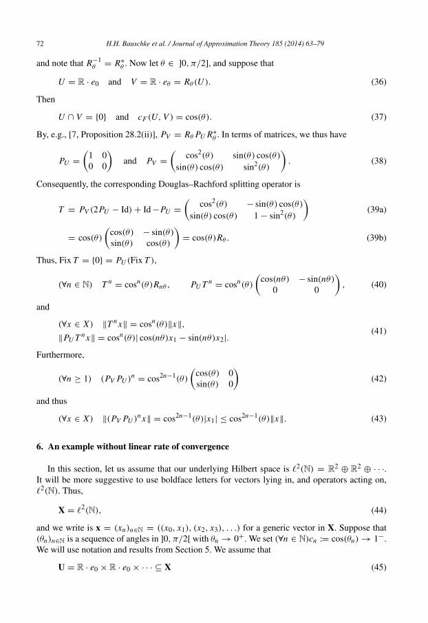
Fig. 1. The distance of the first 100 terms, connected piecewise linearly, of the sequences (T n x)n∈N (red), (PU T n x)n∈N(blue), and ((PV PU )n x)n∈N (green) to the unique solution. (For interpretation of the references to color in this figurelegend, the reader is referred to the web version of this article.)

method appears to be twice as slow as the method of alternating projections. While this iscertainly the case for the iterates (T n x)n∈N, the actual iterates of interest, namely (PU T n x)n∈N,in practice often (somewhat paradoxically) make striking non-monotone progress.

Let us illustrate this using the set up of Section 5 the notation and results of which we willutilize.

Consider first (41) and (43) with x = e0 and θ = π/17. In Fig. 1, we show the first 100 iteratesof the sequences (∥T n x∥)n∈N (red line), (∥PU T n x∥)n∈N (blue line), and (∥(PV PU )n x∥)n∈N(green line). The sequences (∥T n x∥)n∈N and (∥(PV PU )n x∥)n∈N, which are decreasing, representthe distance of the iterates to 0, the unique solution of the problem. While (∥(PV PU )n x∥)n∈Ndecreases faster than (∥T n x∥)n∈N, the sequence of “shadows” (∥PU T n x∥)n∈N exhibits a curiousnon-monotone “rippling” behavior—it may be quite close to the solution soon after the iterationstarts!

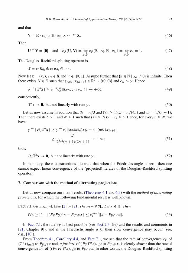
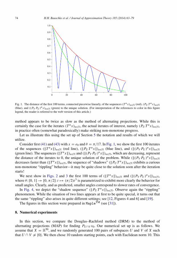
We next show in Figs. 2 and 3 the first 100 terms of (∥T n x∥)n∈N and (∥(PV PU )n x∥)n∈N,where θ : [0, 1] → [0, π/2]: t → (π/2)t3 is parametrized to exhibit more clearly the behavior forsmall angles. Clearly, and as predicted, smaller angles correspond to slower rates of convergence.

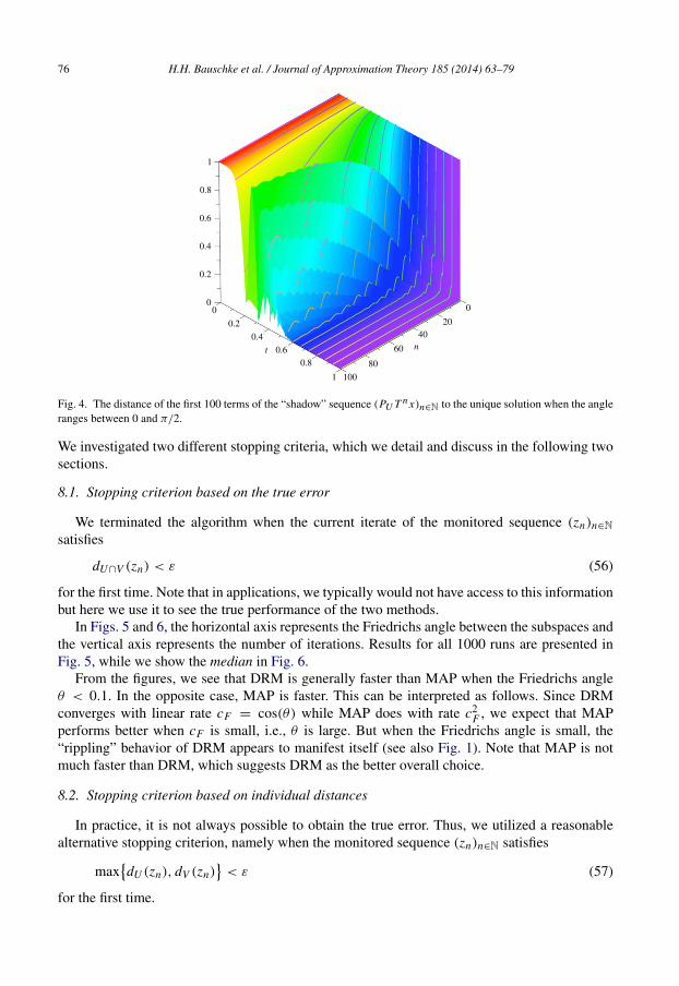
In Fig. 4, we depict the “shadow sequence” (∥PU T n x∥)n∈N. Observe again the “rippling”phenomenon. While the situation of two lines appears at first to be quite special, it turns out thatthe same “rippling” also arises in quite different settings; see [12, Figures 4 and 6] and [19].

The figures in this section were prepared in MapleTM (see [31]).

8. Numerical experiments

In this section, we compare the Douglas–Rachford method (DRM) to the method ofalternating projections (MAP) for finding PU∩V x0. Our numerical set up is as follows. Weassume that X = R50, and we randomly generated 100 pairs of subspaces U and V of X suchthat U ∩ V = {0}. We then chose 10 random starting points, each with Euclidean norm 10. This

H.H. Bauschke et al. / Journal of Approximation Theory 185 (2014) 63–79 75

Fig. 2. The distance of the first 100 terms of the sequence (T n x)n∈N to the unique solution when the angle rangesbetween 0 and π/2.

Fig. 3. The distance of the first 100 terms of the sequence ((PV PU )n x)n∈N to the unique solution when the angle rangesbetween 0 and π/2.

resulted in a total of 1000 instances for each algorithm. Note that the sequences to monitor arePU T n x0

n∈N and

(PV PU )n x0

n∈N (54)

for DRM and for MAP, respectively. Our stopping criterion tolerance was set to

ε := 10−3. (55)

76 H.H. Bauschke et al. / Journal of Approximation Theory 185 (2014) 63–79

Fig. 4. The distance of the first 100 terms of the “shadow” sequence (PU T n x)n∈N to the unique solution when the angleranges between 0 and π/2.

We investigated two different stopping criteria, which we detail and discuss in the following twosections.

8.1. Stopping criterion based on the true error

We terminated the algorithm when the current iterate of the monitored sequence (zn)n∈Nsatisfies

dU∩V (zn) < ε (56)

for the first time. Note that in applications, we typically would not have access to this informationbut here we use it to see the true performance of the two methods.

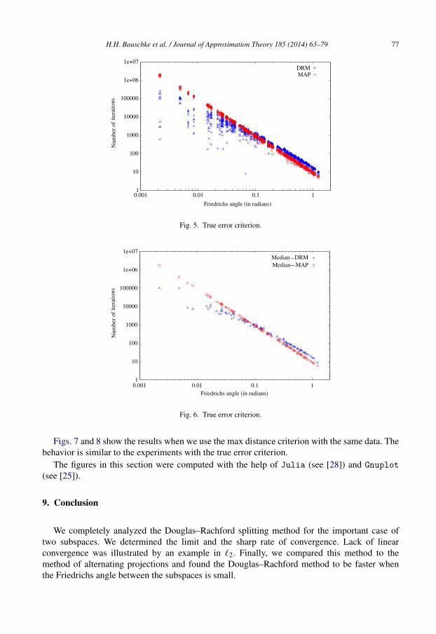
In Figs. 5 and 6, the horizontal axis represents the Friedrichs angle between the subspaces andthe vertical axis represents the number of iterations. Results for all 1000 runs are presented inFig. 5, while we show the median in Fig. 6.

From the figures, we see that DRM is generally faster than MAP when the Friedrichs angleθ < 0.1. In the opposite case, MAP is faster. This can be interpreted as follows. Since DRMconverges with linear rate cF = cos(θ) while MAP does with rate c2

F , we expect that MAPperforms better when cF is small, i.e., θ is large. But when the Friedrichs angle is small, the“rippling” behavior of DRM appears to manifest itself (see also Fig. 1). Note that MAP is notmuch faster than DRM, which suggests DRM as the better overall choice.

8.2. Stopping criterion based on individual distances

In practice, it is not always possible to obtain the true error. Thus, we utilized a reasonablealternative stopping criterion, namely when the monitored sequence (zn)n∈N satisfies

maxdU (zn), dV (zn)

< ε (57)

for the first time.

H.H. Bauschke et al. / Journal of Approximation Theory 185 (2014) 63–79 77

Fig. 5. True error criterion.

Fig. 6. True error criterion.

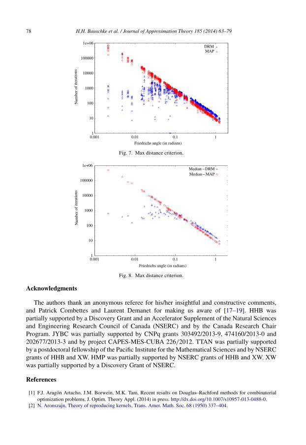
Figs. 7 and 8 show the results when we use the max distance criterion with the same data. Thebehavior is similar to the experiments with the true error criterion.

The figures in this section were computed with the help of Julia (see [28]) and Gnuplot(see [25]).

9. Conclusion

We completely analyzed the Douglas–Rachford splitting method for the important case oftwo subspaces. We determined the limit and the sharp rate of convergence. Lack of linearconvergence was illustrated by an example in ℓ2. Finally, we compared this method to themethod of alternating projections and found the Douglas–Rachford method to be faster whenthe Friedrichs angle between the subspaces is small.

78 H.H. Bauschke et al. / Journal of Approximation Theory 185 (2014) 63–79

Fig. 7. Max distance criterion.

Fig. 8. Max distance criterion.

Acknowledgments

The authors thank an anonymous referee for his/her insightful and constructive comments,and Patrick Combettes and Laurent Demanet for making us aware of [17–19]. HHB waspartially supported by a Discovery Grant and an Accelerator Supplement of the Natural Sciencesand Engineering Research Council of Canada (NSERC) and by the Canada Research ChairProgram. JYBC was partially supported by CNPq grants 303492/2013-9, 474160/2013-0 and202677/2013-3 and by project CAPES-MES-CUBA 226/2012. TTAN was partially supportedby a postdoctoral fellowship of the Pacific Institute for the Mathematical Sciences and by NSERCgrants of HHB and XW. HMP was partially supported by NSERC grants of HHB and XW. XWwas partially supported by a Discovery Grant of NSERC.

References

[1] F.J. Aragon Artacho, J.M. Borwein, M.K. Tam, Recent results on Douglas–Rachford methods for combinatorialoptimization problems, J. Optim. Theory Appl. (2014) in press. http://dx.doi.org/10.1007/s10957-013-0488-0.

[2] N. Aronszajn, Theory of reproducing kernels, Trans. Amer. Math. Soc. 68 (1950) 337–404.

H.H. Bauschke et al. / Journal of Approximation Theory 185 (2014) 63–79 79

[3] J.B. Baillon, R.E. Bruck, S. Reich, On the asymptotic behavior of nonexpansive mappings and semigroups inBanach spaces, Houston J. Math. 4 (1) (1978) 1–9.

[4] H.H. Bauschke, New demiclosedness principles for (firmly) nonexpansive operators, in: Computational andAnalytical Mathematics, Springer, 2013, Chapter 2.

[5] H.H. Bauschke, J.M. Borwein, On projection algorithms for solving convex feasibility problems, SIAM Rev. 38 (3)(1996) 367–426.

[6] H.H. Bauschke, R.I. Bot, W.L. Hare, W.M. Moursi, Attouch–Thera duality revisited: paramonotonicity and operatorsplitting, J. Approx. Theory 164 (2012) 1065–1084.

[7] H.H. Bauschke, P.L. Combettes, Convex Analysis and Monotone Operator Theory in Hilbert Spaces, Springer,2011.

[8] H.H. Bauschke, P.L. Combettes, D.R. Luke, Phase retrieval, error reduction algorithm, and Fienup variants: a viewfrom convex optimization, J. Opt. Soc. Amer. 19 (7) (2002) 1334–1345.

[9] H.H. Bauschke, P.L. Combettes, D.R. Luke, Finding best approximation pairs relative to two closed convex sets inHilbert spaces, J. Approx. Theory 127 (2004) 178–192.

[10] H.H. Bauschke, F. Deutsch, H. Hundal, Characterizing arbitrarily slow convergence in the method of alternatingprojections, Int. Trans. Oper. Res. 16 (2009) 413–425.

[11] H.H. Bauschke, F. Deutsch, H. Hundal, S.-H. Park, Accelerating the convergence of the method of alternatingprojections, Trans. Amer. Math. Soc. 355 (9) (2003) 3433–3461.

[12] H.H. Bauschke, V.R. Koch, Projection Methods: Swiss Army Knives for Solving Feasibility and BestApproximation Problems with Halfspaces, in: Infinite Products and Their Applications, in press.

[13] J.M. Borwein, M.K. Tam, A cyclic Douglas–Rachford iteration scheme, J. Optim. Theory Appl. 160 (2014) 1–29.[14] R.E. Bruck, S. Reich, Nonexpansive projections and resolvents of accretive operators in Banach spaces, Houston J.

Math. 3 (4) (1977) 459–470.[15] Y. Censor, S.A. Zenios, Parallel Optimization, Oxford University Press, 1997.[16] P.L. Combettes, The foundations of set theoretic estimation, Proc. IEEE 81 (2) (1993) 182–208.[17] P.L. Combettes, Iterative construction of the resolvent of a sum of maximal monotone operators, J. Convex Anal.

16 (4) (2009) 727–748.[18] P.L. Combettes, N.N. Reyes, Functions with prescribed best linear approximations, J. Approx. Theory 162 (5)

(2010) 1095–1116.[19] L. Demanet, X. Zhang, Eventual linear convergence of the Douglas–Rachford iteration for basis pursuit, Math.

Comp. (2013) in press. http://arxiv.org/abs/1301.0542v3.[20] F. Deutsch, The angle between subspaces of a Hilbert space, in: S.P. Singh (Ed.), Approximation Theory, Wavelets

and Applications, Kluwer, 1995, pp. 107–130.[21] F. Deutsch, Best Approximation in Inner Product Spaces, Springer, 2001.[22] J. Douglas, H.H. Rachford, On the numerical solution of heat conduction problems in two and three space variables,

Trans. Amer. Math. Soc. 82 (1956) 421–439.[23] J. Eckstein, D.P. Bertsekas, On the Douglas–Rachford splitting method and the proximal point algorithm for

maximal monotone operators, Math. Program. Ser. A 55 (1992) 293–318.[24] V. Elser, I. Rankenburg, P. Thibault, Searching with iterated maps, Proc. Natl. Acad. Sci. 104 (2) (2007) 418–423.[25] GNU Plot, http://sourceforge.net/projects/gnuplot.[26] R. Hesse, D.R. Luke, Nonconvex notions of regularity and convergence of fundamental algorithms for feasibility

problems, SIAM J. Optim. 23 (2013) 2397–2419.[27] R. Hesse, D.R. Luke, P. Neumann, Alternating projections and Douglas–Rachford for sparse affine feasibility,

March 2014, http://arxiv.org/abs/1307.2009v2.[28] The Julia language, http://julialang.org/.[29] S. Kayalar, H. Weinert, Error bounds for the method of alternating projections, Math. Control Signals Systems 1

(1996) 43–59.[30] P.-L. Lions, B. Mercier, Splitting algorithms for the sum of two nonlinear operators, SIAM J. Numer. Anal. 16

(1979) 964–979.[31] Maple, http://www.maplesoft.com/products/maple/.[32] B.F. Svaiter, On weak convergence of the Douglas–Rachford method, SIAM J. Control Optim. 49 (2011) 280–287.