These route descriptions are taken from a variety of sources ...
Upload
independentCategory
view
2download
0
University of Algarve
Department of Electrical Engineering and Computer Science
Signal Processing LABoratory
Matched-Field Processing:
acoustic focalization with data taken in a
shallow water area of the Strait of Sicily
Cristiano Soares
University of Algarve, Faro
March 2001
University of Algarve
Faculty of Science and Technology
Matched-Field Processing:
acoustic focalization with data taken in a
shallow water area of the Strait of Sicily
Cristiano Soares
Department of Electrical Engineering and Computer Science
Signal Processing LABoratory (SiPLAB)
Master of Science Thesisin Underwater Acoustics
March 2001
I
Acknowledgements
I would like to thank to all fellows of SiPLAB the great atmospherein the lab. In particular, I would like to thank Prof. OrlandoRodriguez and Nelson Martins for their availability to listen to meand to discuss many subjects. It was a pleasure to know and towork with Dr. Martin Siderius, who was my supervisor at NATOSACLANTCEN during my participation on the Summer ResearchAssistant programme last summer, and I would like to thank himspecially, for putting the ADVENT’99 acoustic data available tobe included in this thesis. Finally, I would like to thank my thesissupervisor Prof. Dr. Sergio Jesus who played a key role on theprogress of this thesis through our Thursday morning meetings,his great effort during the elaboration of this manuscript, and foradvising me to apply to NATO SACLANTCEN.
II
Abstract
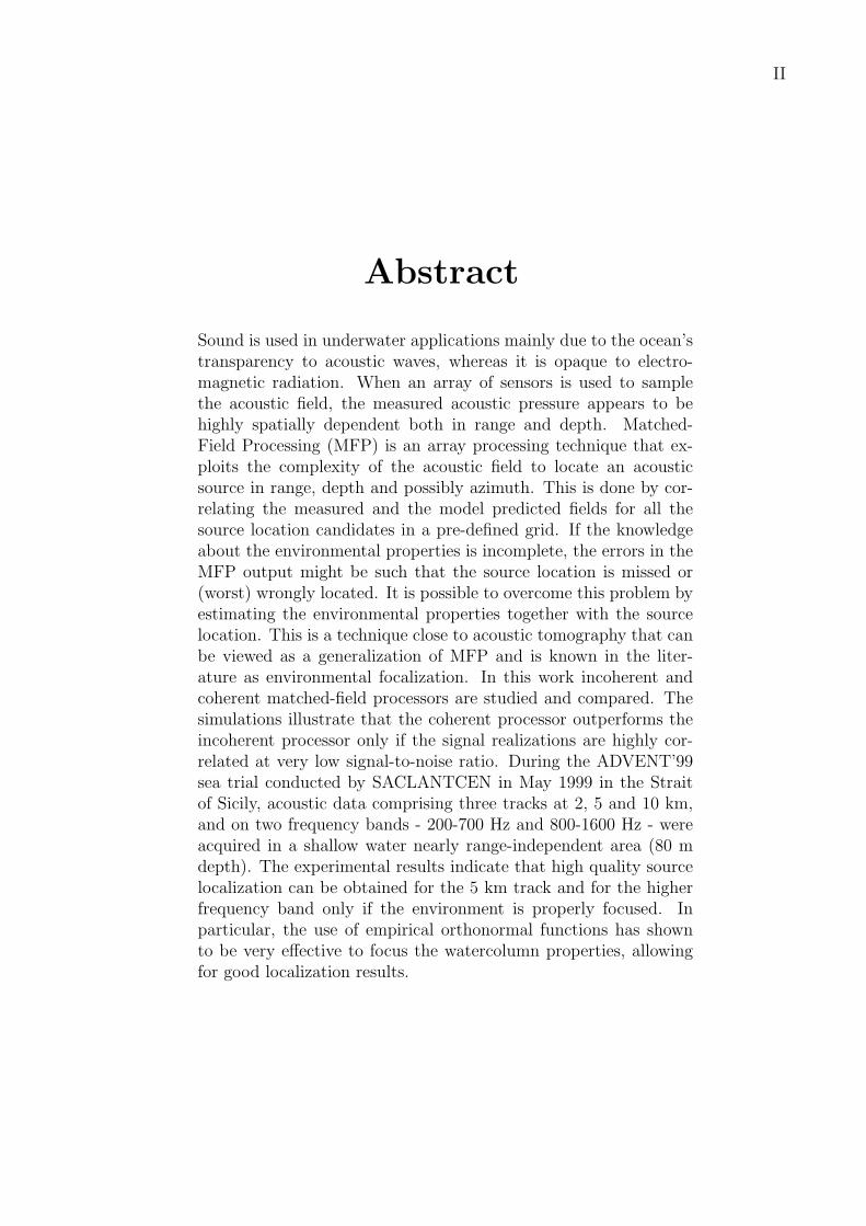
Sound is used in underwater applications mainly due to the ocean’stransparency to acoustic waves, whereas it is opaque to electro-magnetic radiation. When an array of sensors is used to samplethe acoustic field, the measured acoustic pressure appears to behighly spatially dependent both in range and depth. Matched-Field Processing (MFP) is an array processing technique that ex-ploits the complexity of the acoustic field to locate an acousticsource in range, depth and possibly azimuth. This is done by cor-relating the measured and the model predicted fields for all thesource location candidates in a pre-defined grid. If the knowledgeabout the environmental properties is incomplete, the errors in theMFP output might be such that the source location is missed or(worst) wrongly located. It is possible to overcome this problem byestimating the environmental properties together with the sourcelocation. This is a technique close to acoustic tomography that canbe viewed as a generalization of MFP and is known in the liter-ature as environmental focalization. In this work incoherent andcoherent matched-field processors are studied and compared. Thesimulations illustrate that the coherent processor outperforms theincoherent processor only if the signal realizations are highly cor-related at very low signal-to-noise ratio. During the ADVENT’99sea trial conducted by SACLANTCEN in May 1999 in the Straitof Sicily, acoustic data comprising three tracks at 2, 5 and 10 km,and on two frequency bands - 200-700 Hz and 800-1600 Hz - wereacquired in a shallow water nearly range-independent area (80 mdepth). The experimental results indicate that high quality sourcelocalization can be obtained for the 5 km track and for the higherfrequency band only if the environment is properly focused. Inparticular, the use of empirical orthonormal functions has shownto be very effective to focus the watercolumn properties, allowingfor good localization results.
III
Resumo
O som e utilizado em aplicacoes submarinas principalmente dev-ido a transparencia do meio submarino a ondas acusticas enquantoque este e opaco as radiacoes electromagneticas. Quando uma an-tena de sensores e utilizada para amostrar o campo acustico, apressao acustica medida parece ser altamente dependente do espaco,quer em distancia, quer em profundidade. Processamento poradaptacao do campo (em ingles Matched-Field Processing, MFP) euma tecnica de processamento de antenas que explora a complexi-dade do campo acustico para localizar fontes acusticas em distancia,profundidade, e possıvelmente em azimute. Isto e feito correlandoo campo medido com os campos predictos para todas as posicoesda fonte candidatas duma grelha pre-definida. Se o conhecimentosobre as propriedades ambientais for insuficiente, os erros da saıdade MFP poderao ser tais que impossibilitem a localizacao, ou (piorainda) que esta seja errada. E possvel ultrapassar este problema es-timando as propriedades do ambiente conjuntamente com a posicaoda fonte. Esta e uma tecnica que esta proximo da tomografiaacustica que pode ser vista como uma generalizacao do MFP, eque na literatura e conhecida por focalizacao ambiental. Neste tra-balho processadores de adaptacao do campo incoerentes e coerentess ao estudados e comparados. As simulacoes ilustram que o pro-cessador coerente tem um desempenho superior aquele alcanadopelo processador incoerente apenas se as diferentes realizacoes dosinal forem altamente correladas a relacoes sinal-rudo muito baixas.Durante a campanha denominada de ADVENT’99 levada a cabopelo SACLANTCEN em Maio de 1999 no Estreito da Sicilia, dadosacusticos incluindo tres caminhos de propagacao, a 2, 5 e 10 km,e duas bandas de frequencia - 200-700 Hz e 800-1600 Hz - foramadquiridos numa area de aguas pouco profundas praticamente in-dependente da distancia (80 m de profundidade). Os resultadosexperimentais indicam que localizacao de boa qualidade pode serobtida quando a fonte esta a 5 km e para a banda de frequenciasmais altas, so se o ambiente for devidamente focalizado. Em par-ticular, o uso de funcoes empıricas ortonormais mostrou ser muitoeficiente na focalizacao das propriedades propriedades da coluna deagua, permitindo bons resultados de localizacao.
Contents
Acknowledgements I
Abstract II
Resumo III
List of figures VI
1 Introduction 1
2 Acoustic propagation in shallow water 7
3 Matched-Field algorithms 113.1 The Data Model . . . . . . . . . . . . . . . . . . . . . . . . . . . . . . . . . 11
3.1.1 Data model perturbation: the statistical approach . . . . . . . . . . 133.2 Conventional matched-field processing . . . . . . . . . . . . . . . . . . . . . 18
3.2.1 The incoherent conventional processor . . . . . . . . . . . . . . . . . 183.2.2 The coherent conventional processor . . . . . . . . . . . . . . . . . . 203.2.3 The matched-phase coherent processor . . . . . . . . . . . . . . . . . 223.2.4 Efficient implementation of the matched-phase coherent processor . . 23
3.3 Incoherent vs. coherent using synthetic data . . . . . . . . . . . . . . . . . . 273.4 Environmental focalization . . . . . . . . . . . . . . . . . . . . . . . . . . . 30
4 Inverse Problems and Global Optimization using Genetic Algorithms 35
5 The ADVENT’99 sea trial 395.1 Experimental setup . . . . . . . . . . . . . . . . . . . . . . . . . . . . . . . 395.2 The baseline environmental model . . . . . . . . . . . . . . . . . . . . . . . . 40
6 Experimental results: Source localization on the ADVENT’99 data 436.1 Data processing procedure . . . . . . . . . . . . . . . . . . . . . . . . . . . . 436.2 The 2 km track . . . . . . . . . . . . . . . . . . . . . . . . . . . . . . . . . . 44
6.2.1 Optimizing the geometry . . . . . . . . . . . . . . . . . . . . . . . . . 456.3 The 5 km track . . . . . . . . . . . . . . . . . . . . . . . . . . . . . . . . . . 50
6.3.1 Low frequency multi-tones . . . . . . . . . . . . . . . . . . . . . . . . 506.3.2 High frequency tones: blind focalization of main parameters . . . . . 526.3.3 High-frequency tones: A first approach for sound-speed profile focal-
ization . . . . . . . . . . . . . . . . . . . . . . . . . . . . . . . . . . . 546.3.4 High-frequency tones: estimating the sound-speed gradient . . . . . 57
IV

V
6.3.5 High-frequency tones: using empirical orthonormal functions to opti-mize the sound-speed profile . . . . . . . . . . . . . . . . . . . . . . . 60
6.4 The 10 km track . . . . . . . . . . . . . . . . . . . . . . . . . . . . . . . . . 666.5 The 5 km track: Shrinking the array aperture . . . . . . . . . . . . . . . . . 756.6 Testing the matched-phase coherent processor on real data (5 km track) . . . 786.7 Discussion . . . . . . . . . . . . . . . . . . . . . . . . . . . . . . . . . . . . . 82
7 Conclusion 87
List of Figures
3.1 Examples of phase variations in time intervals of 0.5 s for sinusoidal transmis-sions of 800 Hz acquired during the ADVENT’99 sea trial. . . . . . . . . . . 15
3.2 Continuous line: histogram of the phase perturbation in the acoustic dataacquired during the ADVENT’99 experiment. Dashed line: theoretic linewhere the mean is set to -0.136 and the standard deviation to 0.188. . . . . 16
3.3 Continuous lines: density probability functions of the (a) real and (b) imagi-nary parts of complex numbers with uniform phase. Dashed lines: Gaussianfunctions that best fit to the continuous lines. . . . . . . . . . . . . . . . . . 17
3.4 Probability of correct source localization obtained for the incoherent proces-sor (dashed) and the matched-phase processor (continuous) under differentconditions (synthetic data): (a) 4 frequencies and p(ω) = 1; (b) 7 frequen-cies and p(ω) = 1; (c) 16 frequencies and p(ω) = 1; (d) 16 frequencies andcorrelated phase of p(ω) with normal distribution, zero mean and variance0.01; (e) 16 frequencies and uncorrelated phase of p(ω) with normal distribu-tion, zero mean and variance 0.01; (f) 16 frequencies, phase of p(ω) uniformlydistributed and amplitude normally distributed. . . . . . . . . . . . . . . . 29
3.5 Examples of broadband ambiguity surfaces computed for frequencies 300, 400,500 and 600 Hz and SNR equal 0 dB using the a) incoherent processor; b)matched-phase processor . . . . . . . . . . . . . . . . . . . . . . . . . . . . 30
3.6 Matched-field Correlation of the received acoustic signals as a function of fre-quency and time. The data are LFM chirps acquired during the ADVENT’99experiment for the 10 km track. . . . . . . . . . . . . . . . . . . . . . . . . 32
3.7 Range vs. waterdepth ambiguity surface obtained with the broadband conven-tional incoherent processor: (a) Lower frequency set (200-700 Hz);(b) Higherfrequency set (1000-1500 Hz). . . . . . . . . . . . . . . . . . . . . . . . . . . 34
5.1 ITNS Ciclope navigation track carried out during temperature measurements(red curve). The asterisks indicates the positions of the source (blue) and theposition of the array at each day (green). . . . . . . . . . . . . . . . . . . . 40
5.2 Baseline model for the ADVENT’99 experiment. All parameters are range in-dependent. The model assumes the same density and attenuation for sedimentand sub-bottom. . . . . . . . . . . . . . . . . . . . . . . . . . . . . . . . . . 41
5.3 Example of a sound speed profile measured at May 02, 1999 at 06:38. . . . 42
6.1 Ambiguity surfaces obtained for the 2 km track using the higher frequencymulti-tones (between 800 and 1500 Hz) comprising an acquisition time of 8.5hours. The geometric parameters were estimated in a previous step and thegeoacoustic parameters are those in table 5.1. . . . . . . . . . . . . . . . . . 47
VI
VII
6.2 Source localization results over time for the 2 km track using the higher fre-quency multi-tones (800 to 1500 Hz): (a) range; (b) depth. . . . . . . . . . 48
6.3 Bartlett power of the surface main peak over time for the 2 km track usingthe higher frequency multi-tones. . . . . . . . . . . . . . . . . . . . . . . . . 48
6.4 Results of optimization carried out using the higher-frequency multi-tones(800-1500 Hz) in the 2 km track. . . . . . . . . . . . . . . . . . . . . . . . . 49
6.5 Ambiguity surfaces obtained with the broadband conventional incoherent pro-cessor for the 5 km track using the lower frequency multi-tones (200 to 700Hz) taken in a time interval of 6 hours. . . . . . . . . . . . . . . . . . . . . 51
6.6 Ambiguity surfaces obtained with the broadband conventional incoherent pro-cessor for the 5 km track using the higher frequency multi-tones (800 to 1500Hz) taken in a time interval of 6 hours. . . . . . . . . . . . . . . . . . . . . 53
6.7 Ambiguity surfaces obtained with the broadband conventional incoherent pro-cessor for the 5 km track using the higher frequency multi-tones (800 to 1500Hz). In a previous step geometry and sound speed profile depth were focused. 56
6.8 Optimization results for sound speed gradients below 67 m depth for the 5km track by focalization using the higher frequency multi-tones (800 to 1500Hz). . . . . . . . . . . . . . . . . . . . . . . . . . . . . . . . . . . . . . . . . 58
6.9 Ambiguity surfaces for the 5 km track using the higher frequency multi-tones(800 to 1500 Hz). The focalization step included estimation of the gradientof the non-measured sound speed portion. . . . . . . . . . . . . . . . . . . . 59
6.10 Bartlett Power over time for the 5 km track higher frequency multi-tones (800to 1500 Hz). The focalization step included estimation of the gradient of thenon-measured sound speed portion. . . . . . . . . . . . . . . . . . . . . . . 60
6.11 Comparing sound speeds obtained by interpolation of real sound speeds withsound speeds estimated through EOFs using the higher frequency multi-tones(800 to 1500 Hz) at the 5 km track. . . . . . . . . . . . . . . . . . . . . . . 63
6.12 Ambiguity surfaces for the 5 km track using the higher frequency multi-tones(800 to 1500 Hz). The focalization step included estimation of the soundspeed profiles via EOFs. . . . . . . . . . . . . . . . . . . . . . . . . . . . . . 64
6.13 Source localization results over time for the 5 km track using the higher fre-quency multi-tones (800 to 1500 Hz): (a) range; (b) depth. . . . . . . . . . 65
6.14 Bartlett Power over time for the 5 km track using the higher frequency multi-tones (800 to 1500 Hz). The focalization step included estimation of the soundspeed profiles via EOFs. . . . . . . . . . . . . . . . . . . . . . . . . . . . . . 65
6.15 Estimates for (a) range and (b) water depth over time for the 10 km trackusing the lower frequency multi-tones (200 to 700 Hz). Both parameters wereincluded in the same search procedure, resulting in an ambiguous objectivefunction. Both plots have the same shape, suggesting an ambiguity betweenboth parameters. . . . . . . . . . . . . . . . . . . . . . . . . . . . . . . . . . 67
6.16 Ambiguity surfaces obtained with the broadband conventional incoherent pro-cessor for the 10 km track using the lower frequency multi-tones (200 to 700Hz) taken a time interval of 6 hours. 5.1. . . . . . . . . . . . . . . . . . . . 68
6.17 Source localization results over time for the 10 km track using the lower fre-quency multi-tones (200 to 700 Hz): (a) range; (b) depth. . . . . . . . . . . 69
6.18 Bartlett Power over time for the 10 km track using the higher frequency multi-tones (200 to 700 Hz). . . . . . . . . . . . . . . . . . . . . . . . . . . . . . . 69
VIII
6.19 Ambiguity surfaces obtained with the broadband conventional incoherent pro-cessor for the 10 km track using the higher frequency multi-tones (800 to 1500Hz). . . . . . . . . . . . . . . . . . . . . . . . . . . . . . . . . . . . . . . . . 71
6.20 Source localization results over time for the 10 km track using the higherfrequency multi-tones (800 to 1500 Hz): (a) range; (b) depth. . . . . . . . . 72
6.21 Bartlett Power over time for the 10 km track using the higher frequency multi-tones (800 to 1500 Hz). . . . . . . . . . . . . . . . . . . . . . . . . . . . . . 72
6.22 Ambiguity surfaces obtained with the broadband conventional incoherent pro-cessor for the 10 km track using the higher frequency LFM signals (820 to1500 Hz, spaced by 23.4 Hz). . . . . . . . . . . . . . . . . . . . . . . . . . . 73
6.23 Source localization results over time for the 10 km track using the higherfrequency LFM signals (820 to 1500 Hz, spaced by 23.4 Hz): (a) range; (b)depth. . . . . . . . . . . . . . . . . . . . . . . . . . . . . . . . . . . . . . . . 74
6.24 Bartlett Power over time for the 10 km track using the higher frequency LFMsignals (820 to 1500 Hz, spaced by 23.4 Hz). . . . . . . . . . . . . . . . . . . 74
6.25 Source localization results over time for different array apertures using thehigher frequenci multi-tones (800 to 1500 Hz): (a) Range; (b) Depth. Eachcolor stands for a different number of sensors: black for 31; blue for 16; redfor 8; green for 4. . . . . . . . . . . . . . . . . . . . . . . . . . . . . . . . . 77
6.26 Bartlett Power over time for different array apertures using the higher fre-quenci multi-tones (800 to 1500 Hz). Each color stands for a different numberof sensors: black for 31; blue for 16; red for 8; green for 4. . . . . . . . . . . 77
6.27 Source localization results over time for an array aperture of 6 m using thehigher frequency LFM signals (820 to 1500 Hz, spaced by 23.4 Hz) : (a)Range; (b) Depth. . . . . . . . . . . . . . . . . . . . . . . . . . . . . . . . . 77
6.28 Bartlett Power over time for an array aperture of 6 m using the higher fre-quency LFM signals (820 to 1500 Hz, spaced by 23.4 Hz). . . . . . . . . . . 78
6.29 Frequencies selected to study the behaviour of the matched-phase processorusing the 5 km track LFM signals. Each example uses a total of 30 bins:(o)constantly spacing of 23.4; (*) groupings in bands of 7 Hz. . . . . . . . . . . 79
6.30 Ambiguity surfaces obtained by the matched-phase coherent processor for the5 km track using the higher frequency LFM (820 to 1500 Hz, spaced by 23.4Hz). . . . . . . . . . . . . . . . . . . . . . . . . . . . . . . . . . . . . . . . . 81
6.31 Source localization results over time for an array aperture of 14 m using thehigher frequency LFM signals (800 to 1500 Hz, spaced by 23.4 Hz): (a) Range;(b) Depth. (o): equally spaced frequencies; (*) frequencies selected in groups(see fig. 6.29) . . . . . . . . . . . . . . . . . . . . . . . . . . . . . . . . . . . 82
6.32 Bartlett power results over time for an array aperture of 14 m using the higherfrequency LFM signals (800 to 1500 Hz, spaced by 23.4 Hz): (a) Range; (b)Depth. Circles: equally spaced frequencies; asterisks: frequencies selected ingroups (see fig. 6.29) . . . . . . . . . . . . . . . . . . . . . . . . . . . . . . . 82
Chapter 1
Introduction
Underwater acoustics is a scientific discipline that has emerged after the Second World
War and is attracting an ever increasing number of multi-disciplinary scientists all over
the world. Sound is extensively used in undersea applications simply because the ocean is
transparent to the propagation of acoustic waves, whereas it is opaque to the electro-magnetic
waves. Underwater acoustics finds application in a variety of problems that include active
and passive detection and localization of ships and submarines, high resolution imaging,
underwater communications, acoustic tomography, search for buried objects in the seafloor
and remote-sensing of natural phenomena, among many others.
A number of these applications were made possible thanks to the recent increase of com-
putation capabilities of mini and personal computers that allow, in nowadays, to accurately
solve complex differential systems of equations within reasonable time. If these differential
systems of equations properly describe the propagation of sound in the ocean they constitute
what is called an acoustic propagation model and thus a powerful tool for predicting sound
pressure at any designated location, bringing new perspectives to many applications [8]. In
order to be able to solve such complex systems of equations, each model has its own simpli-
fication assumptions since they can not cope with the enormous amount of parameters that
1
2
characterize the such complex environment (the ocean) where the acoustic signal propagates.
One of the applications where acoustic models have been extensively used in the last
thirty years is the passive localization of sound sources. The usage of acoustic models for
source localization was first suggested by Hinich [27] and Bucker [6]. The suggested method
was simply based on the comparison of the acoustic field received on an array with the
acoustic field predicted, by a suitable acoustic model, for the same array but for a given
candidate source position. Varying the source position on the acoustic model would produce
a series of comparison results forming - what is generally called - an ambiguity function. If
the model is sufficiently accurate, relative to the real field, an estimate of the true source
location would be given by the maximum of the ambiguity function. That procedure is
known as Matched-Field Processing (MFP). Since its introduction in the early 70s, MFP
has been intensively studied in many of its aspects (see [2] and references therein).
One of the most important aspects is to determine the impact of incomplete environ-
mental knowledge on the final result. In other words, to quantify what is the necessary
accuracy on the environmental data to obtain a correct source location estimate. Another
similar problem deals with the accuracy to which the geometry of the receiving array should
be known in order to produce a meaningful MFP output. Both missing environmental in-
formation and the lack of knowledge of the relative position of the sensors in the array,
produce what is known as model mismatch and has been the object of a large number of
studies [26, 23, 34, 13, 17]. The bottom line is that the acoustic field is highly dependent on
small errors on the sound speed profile (to the fraction of m/s) and on the water depth as
well as on the sediment properties in shallow water applications [9, 10]. In terms of sensor
position, and as a rule of thumb, sensor depth should be known with an accuracy better than
3
a fifth of wavelength while the error on sensor horizontal displacement should not exceed
half a wavelength [33]. These numbers were drawn from simulated studies and impose severe
limitations for real world applications.
Nevertheless, the first single snapshot source localization results with real data were
shown in [7, 16]. The first consistent results of source localization along time were shown
in [30]. Many other results have been obtained for shallow water data sets [40, 42], in deep
water [18], with horizontal arrays with bottom mounted arrays [35], etc. These results were
made possible also by the usage of specifically designed processors to counter the model
mismatch problem. Conventional methods use the maximum of the correlation between the
measured and predicted fields - that is the Bartlett processor. That is known to be the
optimum estimator of a single source in white noise; however its noise rejection is poor and
with relatively high sidelobes there is little guaranty that the main peak is not overtaken by a
sidelobe upon a small error on the environment or on the array geometry. The processors that
have been proposed along the years can be classified in two categories: those that are designed
to increase sidelobe rejection and those that directly cope with model mismatch in the
model itself. The first category are the so-called high-resolution processors like for instance
minimum variance based [11], the mode-subspace processor [31], the EMV-PC processor
[37] and others. These processors dramatically increase the sidelobe rejection giving very
high and well defined peaks. The advantage is that they provide well defined and exact
estimates even in high noise conditions. Their disadvantage is that they are generally much
more sensitive than the conventional Bartlett processor to model mismatch. The second
category of processors take an approach that built the ”resistance” to model mismatch into
the processor itself. There are at least to well know sub-types of processors in this category:
4
the uncertain processors (OFUP) [45, 43] and the focalization processor [12, 24, 21, 22].
The OFUP processors takes the environmental model parameters as the mean of an a priori
parameter distribution; then a series of conventional processor outputs are generated for a
family of probable models with that distribution. The peak is selected as the OFUP source
location estimate. The focalization processor takes a similar path with, however a significant
difference: the a priori distribution is assumed uniform in a given interval; the model is then
adjusted by searching for the maximum output. Both methods are very computer intensive,
depending on the search space dimension the number of acoustic model forward runs can be
of the order of several thousand.
One important issue with mismatch is that it largely depends on frequency: as frequency
increases it becomes more and more difficult to obtain a suitable match in MFP. For a
number of years MFP was confined to narrowband applications, mainly due to the long
computation time required to calculate the acoustic field at several frequencies. In 1988,
Baggeroer et. all [1] proposed a broadband processor that was combining the results obtained
at each frequency by direct averaging of the respective ambiguity surfaces. This is known
as the incoherent broadband processor, that was shown to correctly determine the source
location with lower sidelobes than its narrowband counterpart. Since then, other broadband
processors have been proposed in the literature creating however some controversy about the
relative advantages and drawbacks of frequency coherent or frequency incoherent processing
[40]. Frequency incoherent processors are those that combine different frequencies without
taking into account their respective phase terms. Generally the terms that are averaged are
the auto-frequency terms that are shown to contain the most part of the energy; however,
the cross-frequency terms do contain a great deal of information for source localization, but
5
their combination requires the knowledge of a phase term for in-phase averaging - this is the
coherent approach [42].
This work directly addresses the coherent versus incoherent controversy by exploring the
properties and extending the efficiency of the recently proposed matched-phase coherent
processor [25]. Its performance on terms of noise rejection is theoretically derived and its
efficiency in various phase distribution contexts is demonstrated by simulated examples. A
simple algorithm is presented to extend its processing capacity to virtually any number of
frequency cross terms instead of the three frequency practical limitations mentioned by the
authors. Another issue raised by this work concerns the performance of the focalization
processor for combating model mismatch in high frequency MFP. This issue is demonstrated
when processing real data acquired during the Advent’99 sea trial performed by SACLANT-
CEN in the Strait of Sicily in May 1999. During this experiment three vertical arrays where
deployed at 2, 5 and 10 km from an acoustic source emitting multi-tones and LFM in two
frequency bands of 200-700 and 800-1600 Hz The environment was nearly range independent
and approximately known at all times. Coherent and incoherent MFP, at low and high fre-
quency, at short and long range, with and without focalization has been tested in this data
set and are shown in this report.
This report is organized as follows: chapter 2 briefly reviews some topics about acoustic
propagation in shallow water like wave equation, normal-modes and ray-solution. In chapter
3 the data model is presented, incoherent and coherent matched-field processors are discussed
and compared with synthetic data. Chapter 4 briefly reviews some fundamental aspects of
inversion problems and optimization. In chapter 5 a brief description of the experimental
setup of the ADVENT’99 sea trial is discussed and the baseline model is presented. In

6
chapter 6 experimental source localization results, based on the estimated forward models
are presented for a source at the three ranges using both frequency bands, are presented and
discussed. Finally in chapter 7 taken from this work are presented.
Chapter 2
Acoustic propagation in shallow water
The wave equation in an ideal fluid can be derived from hydrodynamics and the adiabatic
relation between pressure and density. Considering that the time scale of oceanographic
changes is much longer than the time scale of acoustic propagation, it is assumed that
the material properties density ρ and and sound speed c are independent of time. The
linear approximation of the wave equation involve retaining of only first order terms in the
hydrodynamic equations:
ρ∇(1
ρ∇p)− 1
c2
∂2p
∂t2= 0, (2.1)
where p is the acoustic pressure. Note that this is a homogeneous equation, and that ρ and
c2 are space dependent. Several numerical methods exist to solve this equation. The major
difference between the various techniques is the mathematical manipulation of the wave
equation applied before implementation of the solution. In general the task of implementing
the solution of the wave equation is very dificult due to the complexity of the ocean-acoustic
environment: the sound speed profile is usually non-uniform in depth and range; the sea
surface is rough and time dependent; the ocean floor is typically a very complex and rough
boundary which may be inclined, and its properties are usually varying over range.
7
8
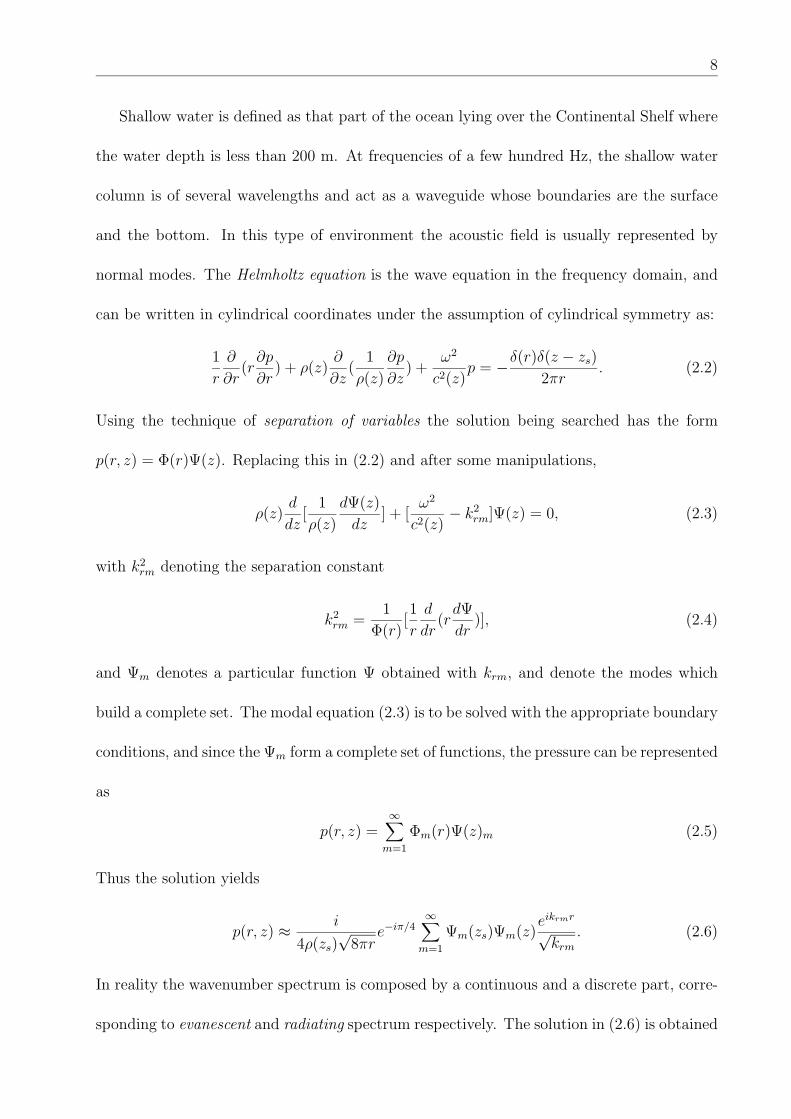
Shallow water is defined as that part of the ocean lying over the Continental Shelf where
the water depth is less than 200 m. At frequencies of a few hundred Hz, the shallow water
column is of several wavelengths and act as a waveguide whose boundaries are the surface
and the bottom. In this type of environment the acoustic field is usually represented by
normal modes. The Helmholtz equation is the wave equation in the frequency domain, and
can be written in cylindrical coordinates under the assumption of cylindrical symmetry as:
1
r
∂
∂r(r∂p
∂r) + ρ(z)
∂
∂z(
1
ρ(z)
∂p
∂z) +
ω2
c2(z)p = −δ(r)δ(z − zs)
2πr. (2.2)
Using the technique of separation of variables the solution being searched has the form
p(r, z) = Φ(r)Ψ(z). Replacing this in (2.2) and after some manipulations,
ρ(z)d
dz[
1
ρ(z)
dΨ(z)
dz] + [
ω2
c2(z)− k2
rm]Ψ(z) = 0, (2.3)
with k2rm denoting the separation constant
k2rm =
1
Φ(r)[1
r
d
dr(rdΨ
dr)], (2.4)
and Ψm denotes a particular function Ψ obtained with krm, and denote the modes which
build a complete set. The modal equation (2.3) is to be solved with the appropriate boundary
conditions, and since the Ψm form a complete set of functions, the pressure can be represented
as
p(r, z) =∞∑m=1
Φm(r)Ψ(z)m (2.5)
Thus the solution yields
p(r, z) ≈ i
4ρ(zs)√
8πre−iπ/4
∞∑m=1
Ψm(zs)Ψm(z)eikrmr√krm
. (2.6)
In reality the wavenumber spectrum is composed by a continuous and a discrete part, corre-
sponding to evanescent and radiating spectrum respectively. The solution in (2.6) is obtained
9
under the assumption that the spectrum is composed only by the discrete part. Hence the
solution is valid only at ranges greater or equal than several water depths away from the
source.
An alternative approximation to the wave equation is the so called ”high frequency
approximation” that consists in representing the acoustic field by the ray solution. The ray
solution of the wave equation is a high frequency approximation, that is useful particularly
for deep water problems, where generally only a few rays are significant. Ray tracing is
satisfactory if the wave length is much less than the length scales in the problem. In shallow
water many significant rays arrive to the receiver, whereas the modes are only a few, which
implies that mode models are preferable to ray tracing models. For ray tracing Snell’s
law provides a simple formula for calculating the ray declination angle when the channel is
modeled as a stratified medium based on the knowledge of the soundspeed at the interface
between to layers.

10
Chapter 3
Matched-Field algorithms
3.1 The Data Model
A signal transmitted by a source, exciting a horizontally stratified, parallel waveguide, is
received by a vertical sensor array and observed during time T . The signals received at each
sensor are included in a vector x(t), for 0 < t ≤ T . The channel is assumed as being linear,
causal, and time-invariant; s(t) is a scalar representing the signal at the source, and h(t) =
h(t, ϑ) is a vector with elements hn(t) representing the channel’s impulse response between
the source and sensor n, i.e., the solution of the Helmholtz equation, also called Green’s
function; u(t) denotes additive stationary noise. Thus x(t) is defined by the convolution
equation:
x(t) =
∞∫0
h(t− τ)s(τ)dτ + u(t). (3.1)
The Fourier transform of the vector h(t) is the transfer function vector H(ω) = H(ω, ϑ)
which is known except for the parameter vector ϑ:
H(ω, ϑ) = [G(ω, ϑ, r1) . . . G(ω, ϑ, rN)]T , (3.2)
where G is the solution of the Helmholtz equation, and ri is a vector that designates the ith
sensors location. To work with finite data portions in the Finite Fourier Transform domain
allows for assumptions of asymptotic distributions for the transformed data for increasing
11
3.1. THE DATA MODEL 12
observation times. It is assumed a band limitation | ω |< Ω for the signal and noise. The
output of the sensors is sampled at a rate ωs > 2Ω, i.e. a sampling period ∆ < π/Ω. The
Fourier Transform is given by
X(ω) = ∆N∑i=1
wT (∆i)x(∆i)e−jω∆i. (3.3)
The window wT (t) is zero outside the interval [0, T ], and normalized,∫∞−∞wT (t)2dt = T .
Thus, (3.1) is written in the frequency domain as
X(ω) = H(ω)S(ω) + U(ω), (3.4)
where S(ω) is the scalar deterministic source waveform, and U(ω) is N(0, σ2UI) distributed.
Note that although no statistical assumption has been made on u(t) (only stationarity has
been assumed), it is possible to assume a distribution for U(ω) - this is a consequence of the
central limit theorem.
In order to model ocean inhomogeneities, a stochastic complex factor p(ω) is introduced
in the signal term leading to
X(ω) = H(ω)S(ω)p(ω) + U(ω), (3.5)
At this point, no considerations are made on the statistical properties of p(ω), and this shall
be discussed later on in more detail. It is defined as
p(ω) = ejφH(ω), (3.6)
where φH(ω) is a random variable whose distribution establishes the distribution of p(ω).
Under the assumption that signal and noise are uncorrelated, noise is uncorrelated from
sensor to sensor, and X(ω) is normally distributed and zero mean, its covariance matrix is
CXX(ω) = E[X(ω)XH(ω)]
= |S(ω)|2H(ω)H(ω)HE|p(ω)|2 + σ2UI. (3.7)
3.1. THE DATA MODEL 13
For some methods it may be important for frequencies 0 < ω1 < ... < ωN < Ω, to have
X(ω1), ..., X(ωN) asymptotically independent. It can be shown that independent random
variables are uncorrelated. For example for methods using cross-frequency correlation it is
required to characterize the moment of second order involving signals at different frequencies.
The noise can be considered as being independent from frequency to frequency, i.e., uncorre-
lated. The same does not happen to the perturbation p(ω), since it represents changes that
occur in the propagation channel, and has a certain impact in the whole spectrum of interest.
It will be assumed that this factor is slowly changing over frequency. Hence the assumption
of high correlation in a limited band may be valid. The cross-frequency covariance matrix
is defined by
CXX(ωi, ωj) = E[X(ωi)XH(ωj)]
= S(ωi)S(ωj)∗H(ωi)H(ωj)
HE[p(ωi)p(ωj)], i 6= j (3.8)
where E[p(ωi)p(ωj)] is the covariance between the perturbations at frequencies ωi and ωj.
Note that cross-frequency covariance resulted in a matrix that contains only a signal compo-
nent: due to the assumption of uncorrelated noise between frequencies, the noise component
has vanished.
3.1.1 Data model perturbation: the statistical approach
Section 3.1 presented the data model that will be used throughout this work. This is the
linear data model, as it usually is assumed. There is one aspect that may be of some
relevance: in the signal term appeared a factor that was called perturbation, and somehow
intends to represent the random features of the channel. Thus, considerations relative to the
statistical properties of this factor should be drawn. Note that in the model, the perturbation

3.1. THE DATA MODEL 14
p(ω) is frequency dependent. Let p be a complex scalar defined as
p = pX + jpY . (3.9)
The question that arises is which is the statistical distribution of the phase of such pertur-
bation. It is commonly accepted to assume the phase o factor p to be uniformly distributed.
Considering the interval between −π2
and π2, for an uniform distribution the mean is zero,
and the variance is π2
12≈ 0.82. Having this in mind it might be illustrative to observe the
real data acquired during the ADVENT’99 Sea Trial to get some insight on this distribution.
Taking the acoustic pressure received by a given sensor during a limited time, the phase at
a certain frequency can be observed.
Fig. 3.1 shows how much the phase increases from one instant to the other on sinusoidal
signals at 800 Hz transmitted during 10 seconds (circles), where measurements are done
for each 0.5 s. These signal were divided into segments of 0.5 seconds, where the first and
the last segments were discarded, hence giving 18 segments. Each of them was Fourier
transformed in order to extract the phase at the frequency of interest. Since the variability
is low, it can be noticed that the phase is approximately linear. It is interesting to obtain
a statistical analysis of this variation in order to get some insight on its distribution. Thus
all the available phase observations were obtained as explained above and consecutive phase
terms were subtracted. In order to obtain the phase what has been called perturbation
these phase differences were subtracted by the slope of the squares line in fig. 3.1. Fig. 3.2
shows the histogram obtained at 800 Hz. The deviation between the measured histogram
(continuous line) and a Gaussian distribution with mean -0.136 and standard deviation of
0.188 radians (dashed line) is minimal. This data set shows some disagreement with what
is commonly assumed: the distribution for the phase perturbation is normal, whereas the
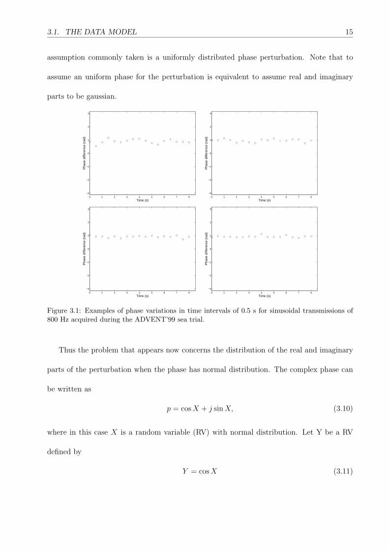
3.1. THE DATA MODEL 15
assumption commonly taken is a uniformly distributed phase perturbation. Note that to
assume an uniform phase for the perturbation is equivalent to assume real and imaginary
parts to be gaussian.
0 1 2 3 4 5 6 7 8
−3
−2
−1
0
1
2
3
Time (s)
Pha
se d
iffer
ence
(ra
d)
0 1 2 3 4 5 6 7 8
−3
−2
−1
0
1
2
3
Time (s)
Pha
se d
iffer
ence
(ra
d)
0 1 2 3 4 5 6 7 8
−3
−2
−1
0
1
2
3
Time (s)
Pha
se d
iffer
ence
(ra
d)
0 1 2 3 4 5 6 7 8
−3
−2
−1
0
1
2
3
Time (s)
Pha
se d
iffer
ence
(ra
d)
Figure 3.1: Examples of phase variations in time intervals of 0.5 s for sinusoidal transmissions of800 Hz acquired during the ADVENT’99 sea trial.
Thus the problem that appears now concerns the distribution of the real and imaginary
parts of the perturbation when the phase has normal distribution. The complex phase can
be written as
p = cosX + j sinX, (3.10)
where in this case X is a random variable (RV) with normal distribution. Let Y be a RV
defined by
Y = cosX (3.11)

3.1. THE DATA MODEL 16
−2 0 2 4 60
0.5
1
1.5
2
2.5
Phase perturbation
Pro
babi
lity
dens
ity
Figure 3.2: Continuous line: histogram of the phase perturbation in the acoustic data acquiredduring the ADVENT’99 experiment. Dashed line: theoretic line where the mean is set to -0.136and the standard deviation to 0.188.
The distribution function of Y is given by
FY (y) = PY ≤ y = PcosX ≤ y = PX ≤ cos−1 y
= FX(cos−1y)
=∫ cos−1 y
−πfX(x)dx, (3.12)
those results were obtained using the definition of the distribution function. Note that
X ∈ [−π, 0], since it is required to have a monotonic growing function in the interval of
interest. Replacing y1 = cos x for x it comes out that dx = (1−y2)−12dy1, and the integration
is made between −1 and y:
FY (y) =∫ y
−1
fX(cos−1 y1)√1− y2
1
dy1, (3.13)
where y ∈ [−1, 1]. Derivating with respect to y, the final probability density function is
obtained:
fY (y) =fX(cos−1 y)√
1− y2. (3.14)
3.1. THE DATA MODEL 17
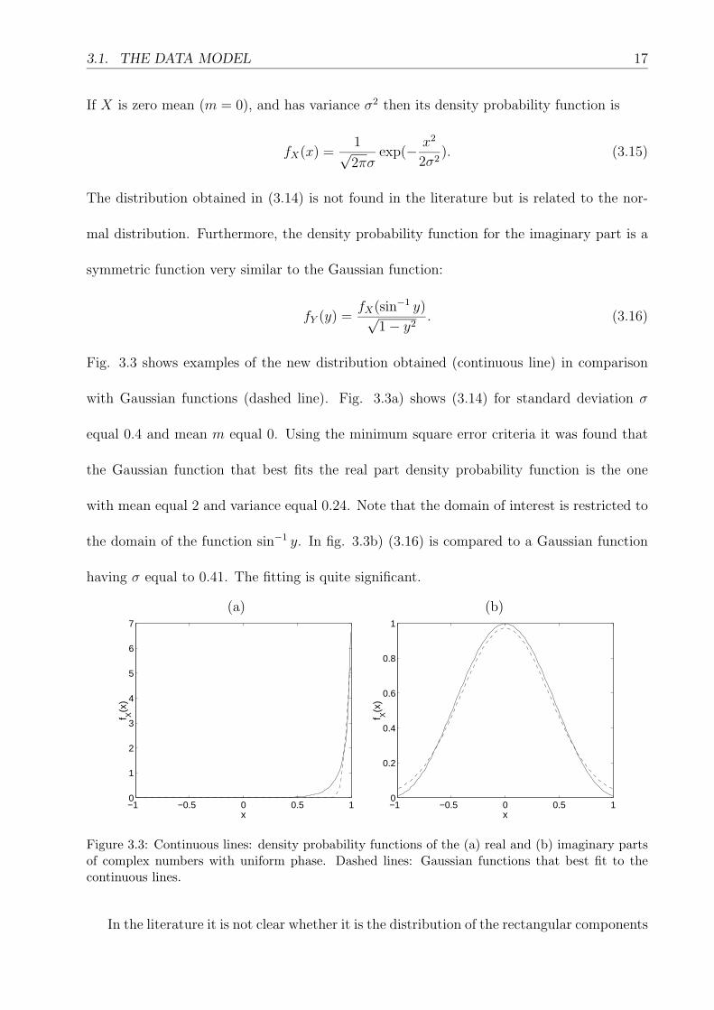
If X is zero mean (m = 0), and has variance σ2 then its density probability function is
fX(x) =1√2πσ
exp(− x2
2σ2). (3.15)
The distribution obtained in (3.14) is not found in the literature but is related to the nor-
mal distribution. Furthermore, the density probability function for the imaginary part is a
symmetric function very similar to the Gaussian function:
fY (y) =fX(sin−1 y)√
1− y2. (3.16)
Fig. 3.3 shows examples of the new distribution obtained (continuous line) in comparison
with Gaussian functions (dashed line). Fig. 3.3a) shows (3.14) for standard deviation σ
equal 0.4 and mean m equal 0. Using the minimum square error criteria it was found that
the Gaussian function that best fits the real part density probability function is the one
with mean equal 2 and variance equal 0.24. Note that the domain of interest is restricted to
the domain of the function sin−1 y. In fig. 3.3b) (3.16) is compared to a Gaussian function
having σ equal to 0.41. The fitting is quite significant.
(a) (b)
−1 −0.5 0 0.5 10
1
2
3
4
5
6
7
x
f X(x
)
−1 −0.5 0 0.5 10
0.2
0.4
0.6
0.8
1
x
f X(x
)
Figure 3.3: Continuous lines: density probability functions of the (a) real and (b) imaginary partsof complex numbers with uniform phase. Dashed lines: Gaussian functions that best fit to thecontinuous lines.
In the literature it is not clear whether it is the distribution of the rectangular components
3.2. CONVENTIONAL MATCHED-FIELD PROCESSING 18
that is independent or whether it is the distribution of the phase. This result suggests that
for practical use, the functions can be considered equivalent, if it is the distribution of the
rectangular distribution that is assumed independently.
3.2 Conventional matched-field processing
3.2.1 The incoherent conventional processor
The incoherent conventional processor, also called linear processor, has been used in almost
every work. The idea is to measure the correlation between the measured field and the
replica field making a linear combination of the acoustic pressure received in each sensor
through the elements of the replica vector:
Y (ω, ϑ) =N∑n=1
w∗n(ω, ϑ)Xn(ω) = wH(ω, ϑ)X(ω), (3.17)
where w is a weighting vector, and Xn is the pressure at sensor n. Basically (3.17) is a
spatially coherent weighted sum of the pressure measured across the sensors. The energy
detector is based on the mean power at the processor output, thus
P (ω) = E|Y (ω, ϑ)|2
= wH(ω, ϑ)E[X(ω)XH(ω)]w(ω, ϑ)
= wH(ω, ϑ)CXX(ω)w(ω, ϑ). (3.18)
The goal now is to determine what is the vector w that maximizes P (ω). To simplify the
notation the dependencies of w and H are supressed. Thus maximization proceeds as follows
maxwwHCXXw = max
wσ2
SwHH HHw + σ2
NwHw
= maxwσ2
S|wHH|2 + σ2N. (3.19)
3.2. CONVENTIONAL MATCHED-FIELD PROCESSING 19
To obtain a non-trivial solution, the norm of w is constrained to 1 when carrying out the
above maximization. In (3.19) the second term is a non-negative constant, thus only the
first term has to be maximized. The estimator for w obtained by maximizing (3.18) is
w =H√HHH
. (3.20)
Taking into account the data model and (3.17) it can be noticed that w is a matched-filter,
since the filter is exactly the normalized channel’s response. However the only thing that is
known is the structure of the filter, remaining the parameter ϑ to be estimated. Finally, and
once the estimator for w has been obtained, it can be placed back into (3.18):
P (ω, ϑ) =HH(ω, ϑ)CXX(ω)H(ω, ϑ)
HH(ω, ϑ)H(ω, ϑ). (3.21)
This processor has into account only one frequency. In the last years it became common to
use the broadband processor [1]:
P (ϑ) =1
K
K∑k=1
HH(ωk, ϑ)CXX(ωk)H(ωk, ϑ)
HH(ωk, ϑ)H(ωk, ϑ). (3.22)
By processing several frequencies together it is expected to obtain a reduction of the variance
of the estimates by reducing the variance of noise, and the estimates obtained are valid for
a band of frequencies - at least in the neighborhood of the frequencies being used [47]. The
sum in (3.22) is carried without having into account the phases of the signals involved in
each correlation term - it is an incoherent processor. In practice only sample covariance
matrices are available:
CXX =L∑l=1
Xl(ω)XlH(ω), (3.23)
therefore an estimate P (ϑ) of (3.22) is obtained.
Later it will be useful to have the matched-field response obtained by the incoherent
3.2. CONVENTIONAL MATCHED-FIELD PROCESSING 20
processor for true parameter ϑ. This is obtained using the data model defined in (3.5), (3.7)
can be replaced in (3.18), and w given by (3.20):
P = wHCXXw
= wH(|S|2H HHE|p|2 + σ2UI)w
= |S|2E|p|2 + σ2Uw
Hw
= |S|2E|p|2 + σ2U . (3.24)
3.2.2 The coherent conventional processor
The previous section presented a processor that takes into account the output of the array’s
sensors in a coherent fashion. However, each term in the summation of (3.22) is a real scalar,
which means that the sum is incoherent. Taking again the data model in (3.5) and the data
vector
XCoh =1
L[X(ω1)T . . . X(ωL)T ]T , (3.25)
a processor that combines coherently different frequencies can be derived. The H(ωi) can
be joined into a vector like:
Hcoh = [HT (ω1), . . . , HT (ωL)]T .
For convenience the vectors H(ωi) have norm equal 1. Now the steps to be followed are
identical to those taken to derive the incoherent estimator (3.17)-(3.20), and the result is
wcoh = Hcoh
3.2. CONVENTIONAL MATCHED-FIELD PROCESSING 21
Note that the covariance matrix in (3.18) is now a block matrix containing the matrices
CXX(ωm, ωn) and is denoted by CcohXX . Replacing again in (3.18) gives:
P (ϑ) = HHcohC
cohXXHcoh
=1
L2
L∑n=1
L∑m=1
H(ωn, ϑ)CXX(ωn, ωm)H(ωm, ϑ) (3.26)
In general, each term is a complex number, except for m = n. But since frequency ωm
is combined with frequency ωn and vice-versa (one correlation term is complex conjugated
of the other), the result of the sum of these two terms is twice the real part of one of the
terms. For example in a range-depth ambiguity surface, it is guaranteed that only for the
true location each term of the sum is a real number, since there is a perfect match between
the measured field and replica field. For all the other locations on the ambiguity surface
each term of the sum will be complex. Hence part of the energy is discarded, reducing the
sidelobes.
In the last part of the previous section the peak value for the true parameter and un-
correlated noise is given by (3.24). The same is done for one term corresponding to the
cross-covariance matrix CXX = CXX(ωi, ωj) of (3.26):
P = wHi CXXwj (3.27)
where wi is the replica for frequency ωi, and CXX is the matrix obtained in (3.8). Replacing
CXX by its form (3.8) as in (3.24), the following result for the power is obtained:
P = SiS∗jE[pip
∗j ], (3.28)
where the indexes i and j are relative to the frequencies ωi and ωi respectively. This result
indicates that if pi e pj are uncorrelated, then the peak will be low. In general the peak for
the coherent processor will be always equal or lower than that obtained by the incoherent
3.2. CONVENTIONAL MATCHED-FIELD PROCESSING 22
processor due to the contribution of the cross-frequency terms and applying the Schwarz
inequality:
E|pi|2 ≥ E[pip∗j ]. (3.29)
The expectance in (3.28) is independent of the parameters ϑ being searched. Hence, all
points in the surface suffer an attenuation by the same factor, i.e., an attenuation of the
main lobe implies an attenuation of the sidelobes. As it was shown in section 3.2.1, the noise
power has a constant contribution over the whole surface, hence increasing the level of the
ambiguity surface by a constant. Further, the number of terms of the coherent processor is
quadratic relative to the number of frequencies, which means that the number of ambiguity
surfaces to average is much larger, which may be an additional factor contributing for sidelobe
reduction.
3.2.3 The matched-phase coherent processor
In section 3.2.2 was developed a coherent processor accounting for frequency coherence.
However, this processor does not account for the phase relationships between frequencies.
In section 3.1 was introduced the data model with a perturbation term p(ω) defined in (3.6)
as a complex exponent. The intention is to model an uncertainty in the phase of H(ω) that
can not be predicted by the model. The idea now is to derive a processor that compensates
these phase uncertainties and simultaneously accounts for the phase relationships between
frequencies. Thus, instead of using simply the replica produced by a propagation model like
that of (3.25), a complex exponential factor is introduced
HMP = [HT (ω1)ejφH(ω1), . . . , HT (ωM)ejφH(ωL)]T ,
in order to compensate the phase obtained the mathematical expectancy in 3.8.
3.2. CONVENTIONAL MATCHED-FIELD PROCESSING 23
Following the same steps as in section 3.2.2, and using (3.30) the matched-phase processor
is obtained:
P (ϑ) = HHMPCcoh
XXHMP
=1
L2
L∑n=1
L∑m=1
HH(ωn, ϑ)CXX(ωn, ωm)H(ωm, ϑ)ej[φH(ωm)−φH(ωn)] (3.30)
This processor works in the same way as the coherent processor shown in section 3.2.2,
however, with the difference that a cross-frequency dependent phase factor φH(ωm)−φH(ωn)
is introduced. Instead of loosing the energy in the imaginary part of each correlation term
in 3.30, this is transferred to the real part. To allow this, it is required that the phase of
the exponent factor is the symmetric phase of the correlation factor. Then all the terms
turn into real numbers, and the sum is carried out in phase. This gives the possibility of
improving the peak-to-sidelobe ratio by adjusting the phase factors. Complex numbers can
be represented in a complex plane as vectors, and it is known that the sum of two vectors
has maximum norm when they have the same direction. In [25] it is suggested to search for
the relative phases as free parameters between 0 and 2π. After the reasoning above this is
not necessary, as it is possible to dramatically restrict the search space. In the next section
a much more efficient implementation of this processor will be shown.
3.2.4 Efficient implementation of the matched-phase coherent pro-cessor
The matched-phase processor treated in section 3.2.3 was presented in [25]. It was mentioned
that the search for the relative phases would be burdensome if the number of frequencies
were greater than three. Also Michalopoulou [42] discusses the possibility of looking for
unknown phases as free parameters, but abandons this strategy for the same reason. The
goal is to look for the phase relationships between different frequencies, i.e. to look for
3.2. CONVENTIONAL MATCHED-FIELD PROCESSING 24
the phases φH(ωi) in (3.30). The number of terms in (3.30) is quadratic with the number of
frequencies, and for each cross-frequency term a phase term is to searched as a free parameter.
Thus, if L is the number of frequencies, the number of free phase terms to be searched is
L(L− 1), increasing rapidly the dimensionality of the search procedure, a side effect that is
not desirable. For illustration, for L = 3 the number of relative phases to be searched is 6,
but if L = 7 then the number of relative phases is already 42. The understanding of how the
processor works gives the possibility of an efficient implementation in order to dramatically
reduce the computational cost. Here, a new approach for calculating the necessary phase
terms is given. First of all one can make use of the following:
p12 = e−i[φ1−φ2]wH1 C12w2,
p13 = e−i[φ1−φ3]wH1 C13w3,
p21 = e−i[φ2−φ1]wH2 C21w1,
p23 = e−i[φ2−φ3]wH2 C23w3,
p31 = e−i[φ3−φ1]wH3 C31w1,
p32 = e−i[φ3−φ2]wH3 C32w2,
where the notation for the cross-frequencies covariance matrix has been changed for conve-
nience to Cij, indicating that frequencies i and j are involved. Thus,
p12 = p∗21
p13 = p∗31
p23 = p∗32.
The sum of a complex number with its conjugate gives twice the real part of the number.
The terms involved in the sum to be carried out are the pij and their complex conjugated.
3.2. CONVENTIONAL MATCHED-FIELD PROCESSING 25
Thus, the sum of all terms is equivalent to the sum of twice the real part of terms where
i < j:
PMP = p12 + p∗21 + p13 + p∗31 + p23 + p∗32
= 2Rep12+ 2Rep13+ 2Rep23. (3.31)
At first sight this seems to be a small gain. However, the number of terms in this sum
increases quadratically with the number of frequencies, hence for a high number of frequencies
this is indeed a significant gain.
But the most important part concerns the search of the relative phases. Assuming a
case where the search is being done in range and depth, it is known that the phases that
maximize the power are symmetric of the phase of the wHi Cijwj, i.e.,
φi − φj = −6 wHi Cijwj (3.32)
where wi and wj are the replicas for the correct location parameters. However, the correct
location parameters are unknown. The first step is to compute ambiguity surfaces,
smnij = wHi Cijwj (3.33)
scanning wi and wj against range and depth. The superscripts m and n stand respectively
for depth and range. After this step, a set of complex numbers is available for each location
(range and depth). It is known that the phase terms that maximize (3.31) are such that the
sij for the correct location are all real numbers. For this specific location, to compute Pmn
(m and n are indexes for range and depth respectively) as defined in (3.31) with the phase
terms that give the maximum is equivalent to
Pmn = 2|wH1 C12w2|+ 2|wH1 C13w3|+ 2|wH2 C23w3|. (3.34)
3.2. CONVENTIONAL MATCHED-FIELD PROCESSING 26
In other words either (3.31) or (3.34) yield the maximum for the same location and for a
certain set of phase terms. Thus, (3.34) can be scanned versus range and depth in order
to obtain its maximum, which leads directly to the phase terms being searched by applying
(3.32) for the Pmn corresponding to the maximum. Let Sij be a matrix corresponding to
the frequencies i and j where the element in column m and n is smnij defined in (3.33), and
Φ a matrix with the phases selected by maximization of (3.34). The final step is to linearly
combine the ambiguity surfaces Sij, and take the maximum:
PMP = max 1
L(L− 1)
L∑ L∑i<j
2ReSijeΦij. (3.35)
The algorithm requires the following steps are taken:
1. Compute the two-frequency ambiguity surfaces for all frequency pairs.
2. Sum the absolute values of the ambiguity surfaces obtained in step 1.
3. Obtain phases corresponding to the maximum obtained in the step 2.
4. Combine ambiguity surfaces through the symmetric of the phases obtained in step 3
(only the real parts multiplied by two).
To look exhaustively for the phase terms would require to take K values in the interval
from 0 to 2π for each frequency. In a case where range and depth were discretized into
respectively M and N samples and for L frequencies, this would result in a search space with
size O = KL ×M × N . With the new approach the phases are determined through direct
inspection of the correlation terms - in the total only two ambiguity surfaces have to be
computed, independently of the number of frequencies.
3.3. INCOHERENT VS. COHERENT USING SYNTHETIC DATA 27
3.3 Incoherent vs. coherent using synthetic data
Sections 3.2.1 and 3.2.2 respectively presented incoherent and coherent conventional matched-
field processors. Section 3.2.3 gives a further development of the coherent processor that
accounts for phase relationship of the acoustic pressure at different frequencies, improving
its ability for sidelobe reduction. While the incoherent processor suffers of high sidelobes if
the noise level is high, the coherent processor has the ability to completely reject the noise,
but on the other hand, it requires the signals at different frequencies to be highly correlated.
Incoherent and coherent processors are tested with synthetic data for different signal-to-
noise ratios, different number of frequencies, and different distributions of the perturbation
phase p(ω). The goal of these tests is to illustrate the conclusion drawn in the previous
paragraph, where the attention goes mainly to the perturbation p(ω), since this determines
whether the different signal realizations are highly correlated or not. The incoherent proces-
sor is compared with the coherent matched-phase processor, where the latter considers only
the cross-frequency terms as done in [25] (m 6= n). This option makes sense, since the sum
of the single-frequency terms by itself is the incoherent processor.
Synthetic data was generated using the SACLANTCEN normal mode propagation model
C-SNAP [15], and the scenario chosen is similar to that in the Strait of Sicily where the
ADVENT’99 sea trial took place. The simulations consider an array of 32 sensors, and
the frequencies range from 300 to 600 Hz. The number of signal realizations generated for
estimating the covariance matrices was 32. To measure the performance of each of these
processors the criteria chosen is the probability of correct source localization versus signal-
to-noise ratio (SNR). SNR varies from values where the probability of localization is zero or
nearly zero, and goes up to values where probability of localization is 1. For each SNR 50
3.3. INCOHERENT VS. COHERENT USING SYNTHETIC DATA 28
trials were done, and then only those where the peak appeared at the exact location were
considered as yielding the correct result.
First, and as a consequence of the requirement of the coherent processor, the data model
in (3.4) was considered. This is equivalent to the model in (3.5) with p(ω) = 1 with proba-
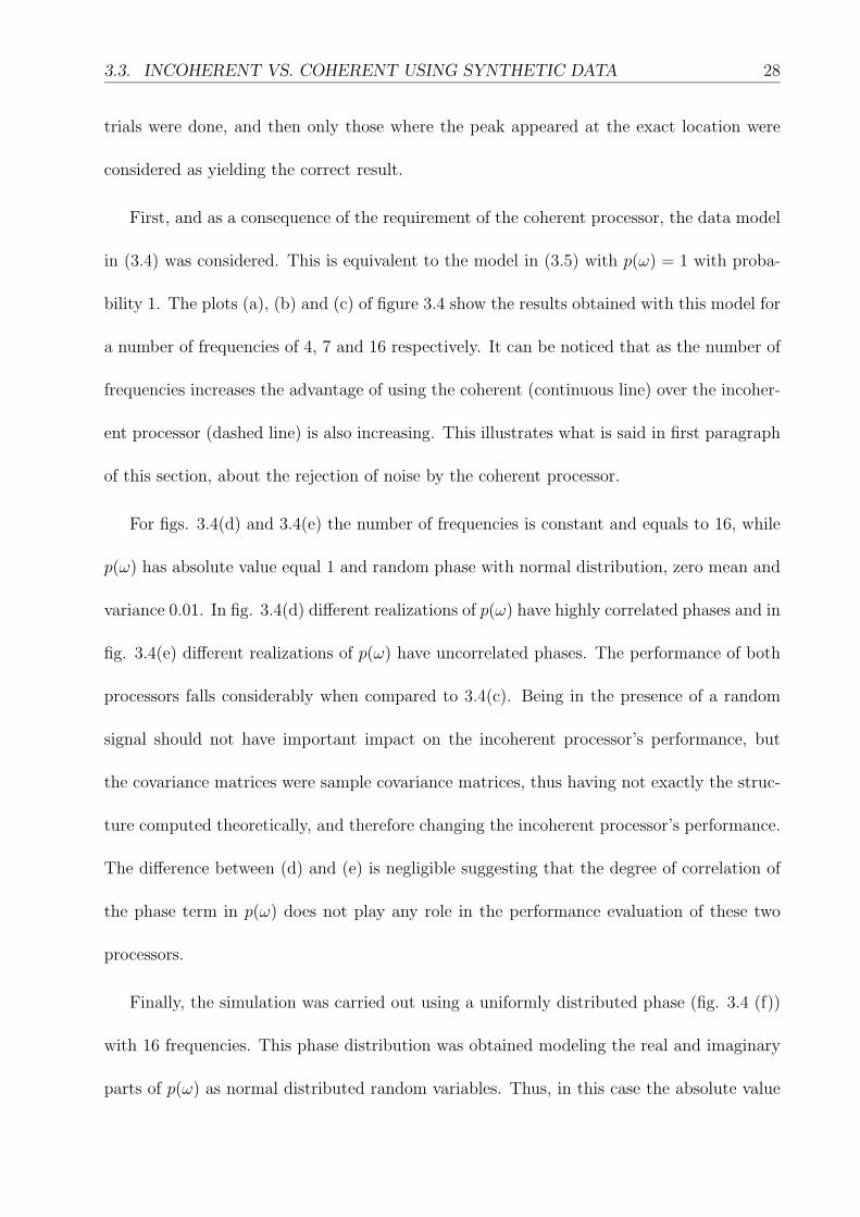
bility 1. The plots (a), (b) and (c) of figure 3.4 show the results obtained with this model for
a number of frequencies of 4, 7 and 16 respectively. It can be noticed that as the number of
frequencies increases the advantage of using the coherent (continuous line) over the incoher-
ent processor (dashed line) is also increasing. This illustrates what is said in first paragraph
of this section, about the rejection of noise by the coherent processor.
For figs. 3.4(d) and 3.4(e) the number of frequencies is constant and equals to 16, while
p(ω) has absolute value equal 1 and random phase with normal distribution, zero mean and
variance 0.01. In fig. 3.4(d) different realizations of p(ω) have highly correlated phases and in
fig. 3.4(e) different realizations of p(ω) have uncorrelated phases. The performance of both
processors falls considerably when compared to 3.4(c). Being in the presence of a random
signal should not have important impact on the incoherent processor’s performance, but
the covariance matrices were sample covariance matrices, thus having not exactly the struc-
ture computed theoretically, and therefore changing the incoherent processor’s performance.
The difference between (d) and (e) is negligible suggesting that the degree of correlation of
the phase term in p(ω) does not play any role in the performance evaluation of these two
processors.
Finally, the simulation was carried out using a uniformly distributed phase (fig. 3.4 (f))
with 16 frequencies. This phase distribution was obtained modeling the real and imaginary
parts of p(ω) as normal distributed random variables. Thus, in this case the absolute value

3.3. INCOHERENT VS. COHERENT USING SYNTHETIC DATA 29
(a) (d)
−20 −15 −10 −5 00
0.1
0.2
0.3
0.4
0.5
0.6
0.7
0.8
0.9
1
SNR (dB)
Pro
babi
lity
−20 −15 −10 −5 00
0.1
0.2
0.3
0.4
0.5
0.6
0.7
0.8
0.9
1
SNR (dB)
Pro
babi
lity
(b) (e)
−20 −15 −10 −5 00
0.1
0.2
0.3
0.4
0.5
0.6
0.7
0.8
0.9
1
SNR (dB)
Pro
babi
lity
−20 −15 −10 −5 00
0.1
0.2
0.3
0.4
0.5
0.6
0.7
0.8
0.9
1
SNR (dB)
Pro
babi
lity
(c) (f)
−20 −15 −10 −5 00
0.1
0.2
0.3
0.4
0.5
0.6
0.7
0.8
0.9
1
SNR (dB)
Pro
babi
lity
−20 −15 −10 −5 00
0.1
0.2
0.3
0.4
0.5
0.6
0.7
0.8
0.9
1
SNR (dB)
Pro
babi
lity
Figure 3.4: Probability of correct source localization obtained for the incoherent processor (dashed)and the matched-phase processor (continuous) under different conditions (synthetic data): (a) 4frequencies and p(ω) = 1; (b) 7 frequencies and p(ω) = 1; (c) 16 frequencies and p(ω) = 1; (d) 16frequencies and correlated phase of p(ω) with normal distribution, zero mean and variance 0.01; (e)16 frequencies and uncorrelated phase of p(ω) with normal distribution, zero mean and variance0.01; (f) 16 frequencies, phase of p(ω) uniformly distributed and amplitude normally distributed.
3.4. ENVIRONMENTAL FOCALIZATION 30
of p(ω) is no longer equal 1 and is a random variable too. The comparison shows that under
this conditions the incoherent processor has higher ability to localize the source than the
coherent processor. Attending to (3.8), this result suggests that the SNR obtained by the
coherent processor is very low, forcing it to fail to localize more often than the incoherent
processor. Note that these tests use sample matrices, hence the noise is not completely
rejected.
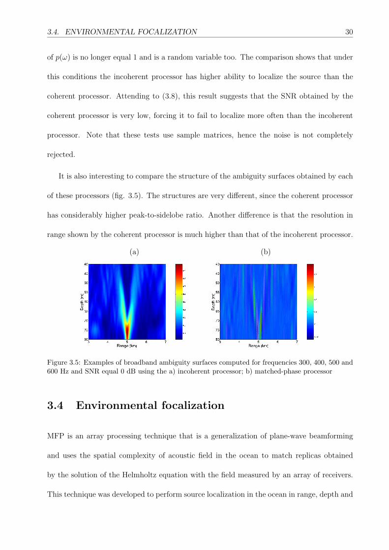
It is also interesting to compare the structure of the ambiguity surfaces obtained by each
of these processors (fig. 3.5). The structures are very different, since the coherent processor
has considerably higher peak-to-sidelobe ratio. Another difference is that the resolution in
range shown by the coherent processor is much higher than that of the incoherent processor.
(a) (b)
Figure 3.5: Examples of broadband ambiguity surfaces computed for frequencies 300, 400, 500 and600 Hz and SNR equal 0 dB using the a) incoherent processor; b) matched-phase processor
3.4 Environmental focalization
MFP is an array processing technique that is a generalization of plane-wave beamforming
and uses the spatial complexity of acoustic field in the ocean to match replicas obtained
by the solution of the Helmholtz equation with the field measured by an array of receivers.
This technique was developed to perform source localization in the ocean in range, depth and
3.4. ENVIRONMENTAL FOCALIZATION 31
azimuth, provided that the environment of the propagation channel is known with sufficient
accuracy. The amount of information available about the environment is a serious problem
to deal with in MFP. The propagation model that solves the Helmholtz equation is fed with
the parameters of the environment, and returns the replica field having into account those
parameters and a given source position. To properly localize the source it is required to know
the environmental parameters with enough accuracy. This is not always possible. Seafloor
properties in shallow water are often characterized by strong variability, and the employment
of seismic surveying and coring for exploring extensive areas is, in general, a very expensive
and time consuming task. Another issue is time coherence of the environment. For example,
if a source is to be located along time, or a moving source is to be tracked, important changes
in the environment may occur over time. In fig. 3.6 the ADVENT’99 data set was used to
show how acoustic data decorrelate over time for a period of 5 hours. The available LFM
transmissions, comprising the band from 200 to 1600 Hz, were Fourier transformed and
analyzed as follows: for each frequency a series of data segments received along time at the
vertical array are compared to a reference segment. This is done by computing the absolute
value of the internal vector product between the reference pressure vector and the other
pressure vectors. As time elapses, the data becomes less correlated. This reflects changes
in the environment - geoacoustic parameters, oceanografic parameters like temperatures, or
internal waves do change in a periodic fashion. It can be observed that the field decorrelates
faster and more at higher frequencies.
Focalization is a generalization of matched-field processing, in which both the source
parameters and the environmental parameters are equally searched. Environmental focal-
ization provides a powerful solution for the lack of accurate measures of the environmental

3.4. ENVIRONMENTAL FOCALIZATION 32
(a) (b)
Figure 3.6: Matched-field Correlation of the received acoustic signals as a function of frequencyand time. The data are LFM chirps acquired during the ADVENT’99 experiment for the 10 kmtrack.
parameters, and to overcome mismatch.
An important concept that rises often in environmental focalization is ”the equivalent
model”. Two models are equivalent if they are different in geometry, environmental pa-
rameters or range-dependence, while giving a similar acoustic response. For example, very
few works were done under assumptions of range-dependence. In fact a range-independent
environment does not exist. Over a few kilometers it is unlikely that bathymetry, seafloor
properties, or even temperature in the water column are constant. The concept of equivalent
models allows simplification of the modeling process by the use of an environmental model
that has different parameters, while giving a similar acoustic response.
In some cases it is not possible to assume range-independence. This is shown by Gerstoft
et. al. [21] with real data acquired during the North Elba Sea Trial in October 1993
conducted by SACLANTCEN. Two data sets, with central frequencies of 170 and 335 Hz
respectively, were available. Optimization of only geometric and geoacoustic parameters in a
range-independent environment was found to be satisfactory at the lower frequencies, but for
the higher frequencies optimization of additional parameters by inclusion of either a range
3.4. ENVIRONMENTAL FOCALIZATION 33
dependent bathymetry or ocean sound speed profile was essential for a successful inversion.
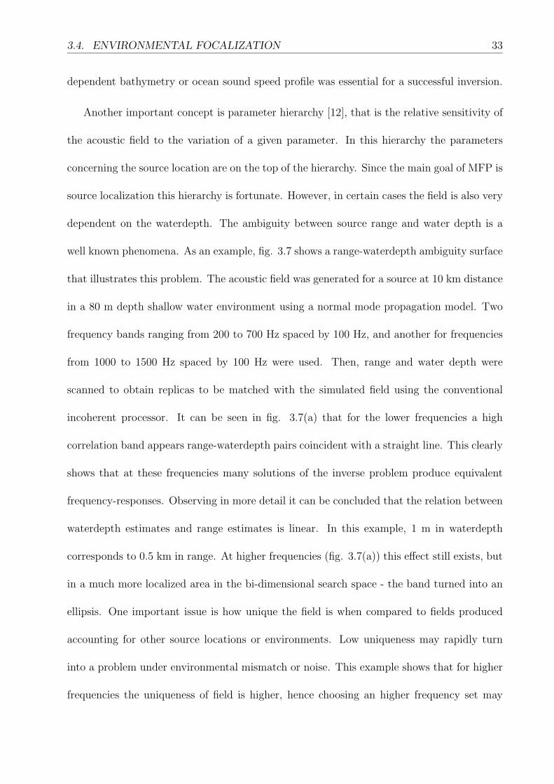
Another important concept is parameter hierarchy [12], that is the relative sensitivity of
the acoustic field to the variation of a given parameter. In this hierarchy the parameters
concerning the source location are on the top of the hierarchy. Since the main goal of MFP is
source localization this hierarchy is fortunate. However, in certain cases the field is also very
dependent on the waterdepth. The ambiguity between source range and water depth is a
well known phenomena. As an example, fig. 3.7 shows a range-waterdepth ambiguity surface
that illustrates this problem. The acoustic field was generated for a source at 10 km distance
in a 80 m depth shallow water environment using a normal mode propagation model. Two
frequency bands ranging from 200 to 700 Hz spaced by 100 Hz, and another for frequencies
from 1000 to 1500 Hz spaced by 100 Hz were used. Then, range and water depth were
scanned to obtain replicas to be matched with the simulated field using the conventional
incoherent processor. It can be seen in fig. 3.7(a) that for the lower frequencies a high
correlation band appears range-waterdepth pairs coincident with a straight line. This clearly
shows that at these frequencies many solutions of the inverse problem produce equivalent
frequency-responses. Observing in more detail it can be concluded that the relation between
waterdepth estimates and range estimates is linear. In this example, 1 m in waterdepth
corresponds to 0.5 km in range. At higher frequencies (fig. 3.7(a)) this effect still exists, but
in a much more localized area in the bi-dimensional search space - the band turned into an
ellipsis. One important issue is how unique the field is when compared to fields produced
accounting for other source locations or environments. Low uniqueness may rapidly turn
into a problem under environmental mismatch or noise. This example shows that for higher
frequencies the uniqueness of field is higher, hence choosing an higher frequency set may
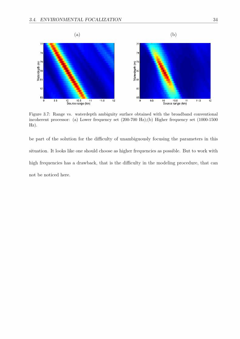
3.4. ENVIRONMENTAL FOCALIZATION 34
(a) (b)
Figure 3.7: Range vs. waterdepth ambiguity surface obtained with the broadband conventionalincoherent processor: (a) Lower frequency set (200-700 Hz);(b) Higher frequency set (1000-1500Hz).
be part of the solution for the difficulty of unambiguously focusing the parameters in this
situation. It looks like one should choose as higher frequencies as possible. But to work with
high frequencies has a drawback, that is the difficulty in the modeling procedure, that can
not be noticed here.

Chapter 4
Inverse Problems and GlobalOptimization using GeneticAlgorithms
Determining the range and depth location of an acoustic source in a waveguide from the
acoustic field measured on a vertical array of sensors can be seen as an inverse problem.
The same applies when estimating the environmental parameters of a waveguide from the
receiver acoustic field. Inverse problems are common to many areas of physics and functional
analysis. Generic methodologies and algorithms are also applicable to our problem and will
not be explained here in detail.
As a generic concept, inverse problems can be classified as well behaved or ill conditioned.
Well behaved inverse problems are generally linear, analytical and allow a solution that is
unique. In our case the derivation of the acoustic field in given environmental and genetic
conditions is non-linear and non-analytical, moreover, since the received field is contaminated
with noise there is no guaranty of uniqueness.
For such a ill conditioned inverse problem, the corresponding multi-dimensional objective
function may exhibit several maxima among which the highest may not correspond to the
true solution. In the last 10 years a number of techniques have been proposed in the literature
35
36
to cope with such optimization problems [39]. Among these techniques, Genetic Algorithm
(GA) is a class of stochastic methods that have the following characteristics:
• perform global optimization;
• are able to escape from local extrema;
• have convergence to the true solution.
The GA is an optimization method based on principles of biological evolution of indi-
viduals [28]. An individual is a collection of bit chains that represents one of the possible
parameter vectors, and a population is a set of individuals that evolves through time as gen-
erations. A generation is an iteration in which the fitness of each individual is computed by
the so-called objective function. The fitness represents the ”quality” of an individual. The
probability of an individual to be included into the next generation depends on its fitness,
i.e. individuals with higher fitness are more likely to survive. Two probabilistic operators are
applied to the individuals: the crossover operator and the mutation operator. The crossover
operator joins individuals into pairs without considering their fitness, and a given number
of bits is exchanged with a given probability. The mutation operator inverts every bit with
a given probability. This operator is important to avoid the loss of individuals’ variety. The
loss of variety of individuals can lead to convergence to local extrema. Therefore the muta-
tion probability should be set high enough to keep the search algorithm being able to escape
from local maxima but low enough to not slowdown convergence to the global extremum,
thus it is a compromise between speed and accuracy. At the beginning a random population
of all possible vectors is selected. The fitness of each individual is computed. The operators
crossover and mutation are applied to get a new population - the children. The fitness is
37
improved from generation to generation through evolutionary mechanisms. An evolutionary
step consists of selection of individuals based on individuals’ fitness.
Global optimization will be applied to the matched-field procedure for the focalization
of the geometry environment. The replica fields are obtained with the normal mode prop-
agation model C-SNAP [15] feeding in the forward model parameters of the geometry and
environment. The inverse problem corresponds to the estimation of the geometric and envi-
ronmental parameters. To achieve this an objective function has to be evaluated, which is
the conventional Bartlett processor that correlates the replicas with the measured field. This
function has to be maximized in order to determine the estimated parameters. To achieve
this maximization a GA implemented by Tobias Fassbender [14] has been used.
The GA is able to reach the maximum by sampling a very small number of points of the
objective function which, in the case of MFP, allows the inversion of problems that would
be unsolvable using traditional methods.

38

Chapter 5
The ADVENT’99 sea trial
5.1 Experimental setup
The SACLANT Undersea Research Centre and TNO-FEL conducted a sea trial in order
to acquire acoustic data on the Adventure Bank off the southwest coast of Sicily (Italy)
in May 1999. This area has a low range-dependence, and was found to be favorable for
acoustic propagation. The data were acquired during the first three days of May. The
acoustic source was mounted on a moored tower 4 m off the bottom at a depth of 76 m.
The signals were received by an acoustic array of 64 elements. Each day it was deployed at
different ranges of 2, 5, and 10 km. Broadband acoustic linear frequency modulated signals
and multi-tones were transmitted every minute. To accomplish this, two sources were used,
one for lower frequencies (200-700 Hz), and another for higher frequencies (800-1600 Hz).
The transmission time was around 5 hours for the 2 and 5 km tracks, and 18 hours for the
10 km track.
For sound speed measurements a 49-element Conductivity-Temperature-Depth (CTD)
chain towed by ITNS Ciclope with a data sampling every 2 s was used. The CTD chain
spanned around 80% of the water column, and was towed continuously between the acoustic
source and the vertical array (10 km track) during all transmissions in a parallel line to the
39

5.2. THE BASELINE ENVIRONMENTAL MODEL 40
Figure 5.1: ITNS Ciclope navigation track carried out during temperature measurements (redcurve). The asterisks indicates the positions of the source (blue) and the position of the array ateach day (green).
acoustic transmission path (fig. 5.1).
5.2 The baseline environmental model
The baseline model consisted of an ocean layer overlying a sediment layer and a bottom
half space, assumed to be range independent, as shown on fig. 5.2. For the purposes of the
inversion the forward model parameters were divided into four parameter subsets: geometric,
sediment, bottom, and water sound speed. The geometric parameters included source range,
source depth, receiver depth and bathymetry. The baseline sediment and bottom properties
used for the ADVENT site were those estimated by Siderius [46] using the low frequency
data (see table 5.1).
Fig. 5.3 shows an example of sound speed profile measured close to the array 5 km
distance from the source at May 02, at 06:38. This is a typical double termocline profile at
10 m and 55 m depth with isovelocity layers in between.
The acoustic array had 64 receiving elements with different spacings, but throughout this
work only the sensors spaced by 2 m are used giving a maximum of 31 sensors and an array
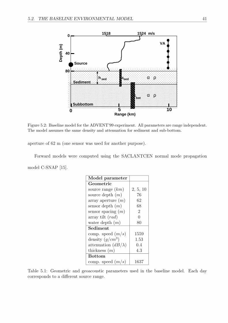
5.2. THE BASELINE ENVIRONMENTAL MODEL 41
0
40
80
Dep
th (
m)
Range (km)
Source
Sediment
Subbottom
h sed csed
cbot
VA
α ρ
α ρ
0 5 10
1518 1524 m/s
Figure 5.2: Baseline model for the ADVENT’99 experiment. All parameters are range independent.The model assumes the same density and attenuation for sediment and sub-bottom.
aperture of 62 m (one sensor was used for another purpose).
Forward models were computed using the SACLANTCEN normal mode propagation
model C-SNAP [15].
Model parameterGeometricsource range (km) 2, 5, 10source depth (m) 76array aperture (m) 62sensor depth (m) 68sensor spacing (m) 2array tilt (rad) 0water depth (m) 80Sedimentcomp. speed (m/s) 1559density (g/cm3) 1.53attenuation (dB/λ) 0.4thickness (m) 4.3Bottomcomp. speed (m/s) 1637
Table 5.1: Geometric and geoacoustic parameters used in the baseline model. Each daycorresponds to a different source range.
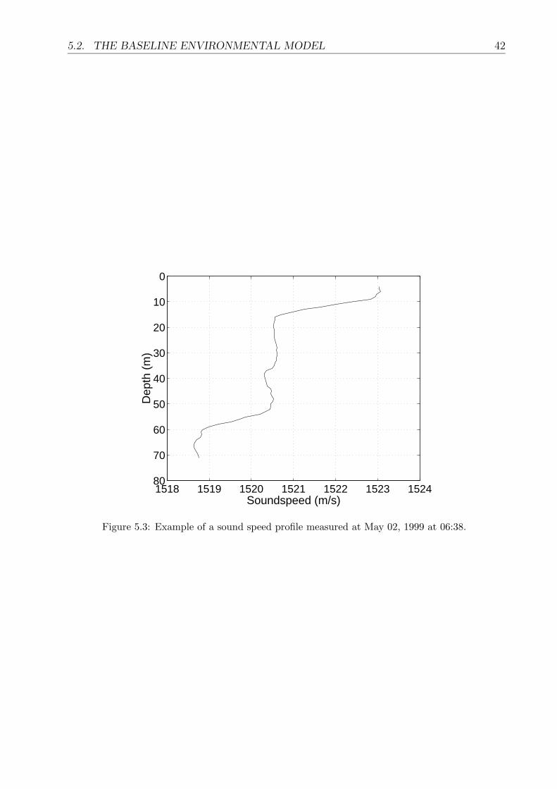
5.2. THE BASELINE ENVIRONMENTAL MODEL 42
1518 1519 1520 1521 1522 1523 1524
0
10
20
30
40
50
60
70
80
Soundspeed (m/s)
Dep
th (
m)
Figure 5.3: Example of a sound speed profile measured at May 02, 1999 at 06:38.
Chapter 6
Experimental results: Sourcelocalization on the ADVENT’99 data
6.1 Data processing procedure
This section is to explain what is the general procedure applied on the data analysis for
source localization on the three tracks in the next sections. The algorithm is divided in 2
steps:
• focalization of the geometry and environment;
• source localization.
The focalization of the environment and geometry (step 1) was posed as an optimization
problem, that is to find a vector of parameters θ that maximizes an objective function,
which in this case is the conventional incoherent processor obtained in (3.22). To successfully
achieve the goal of this step a GA is used. The primary aim of this step is to determine the
environment and parameters concerning the array. Therefore, the source location parameters
are searched in narrow intervals.
Step 2 is range-depth source localization. The environment is fixed to the parameters
obtained in step 1 and range-depth ambiguity surfaces are computed.
43
6.2. THE 2 KM TRACK 44
Throughout this work mostly the multi-tones will be used, which had the following
frequencies:
• Lower frequencies comprising the interval ranging from 200 to 700 Hz, spaced by 100
Hz, i.e. 6 bins were used.
• Higher frequencies comprising the interval from 800 to 1500 Hz, where the bins were
800, 900, 1000, 1200, 1400 and 1500 Hz.
To compute the covariance matrix in (3.7), a single ping of 10 s was divided into 0.5 s
segments, where the first and last segments were discarded, and then Fourier transformed.
Thus, each covariance matrix is the average of 18 outer products.
6.2 The 2 km track
The first data to be analyzed is obviously that acquired on the 2 km track. The environ-
mental parameters are those estimated for the 2 km lower frequency multi-tones by Siderius
[46] and shown in table 5.2. The sound-speed profiles available for this day correspond to
those measured close to the array (the times are shown in table 6.1). Since for this track
the low-frequency has been already analyzed, only the higher-frequency data is going to be
analyzed. In the focalization step were included only geometric parameters. Table 6.2 show
the search boundaries and quantization steps taken when optimizing with the GA. The num-
ber of iterations was set to 40 with populations of 100 individuals. Crossover and mutation
probabilities were set to 0.9 and 0.011 respectively. Note that all these values related to
the GA parameters are canonical and had to be slightly re-adjusted for the optimizations in
other ranges.
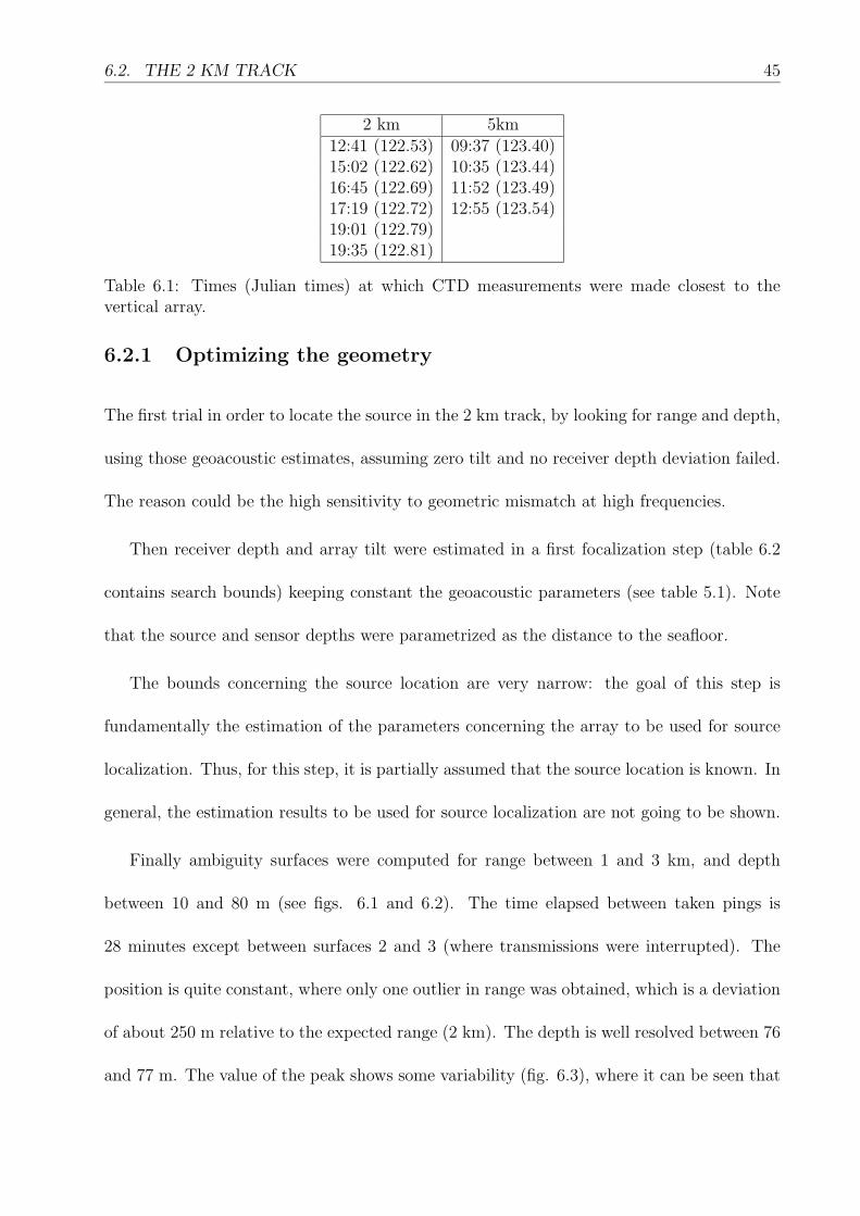
6.2. THE 2 KM TRACK 45
2 km 5km12:41 (122.53) 09:37 (123.40)15:02 (122.62) 10:35 (123.44)16:45 (122.69) 11:52 (123.49)17:19 (122.72) 12:55 (123.54)19:01 (122.79)19:35 (122.81)
Table 6.1: Times (Julian times) at which CTD measurements were made closest to thevertical array.
6.2.1 Optimizing the geometry
The first trial in order to locate the source in the 2 km track, by looking for range and depth,
using those geoacoustic estimates, assuming zero tilt and no receiver depth deviation failed.
The reason could be the high sensitivity to geometric mismatch at high frequencies.
Then receiver depth and array tilt were estimated in a first focalization step (table 6.2
contains search bounds) keeping constant the geoacoustic parameters (see table 5.1). Note
that the source and sensor depths were parametrized as the distance to the seafloor.
The bounds concerning the source location are very narrow: the goal of this step is
fundamentally the estimation of the parameters concerning the array to be used for source
localization. Thus, for this step, it is partially assumed that the source location is known. In
general, the estimation results to be used for source localization are not going to be shown.
Finally ambiguity surfaces were computed for range between 1 and 3 km, and depth
between 10 and 80 m (see figs. 6.1 and 6.2). The time elapsed between taken pings is
28 minutes except between surfaces 2 and 3 (where transmissions were interrupted). The
position is quite constant, where only one outlier in range was obtained, which is a deviation
of about 250 m relative to the expected range (2 km). The depth is well resolved between 76
and 77 m. The value of the peak shows some variability (fig. 6.3), where it can be seen that
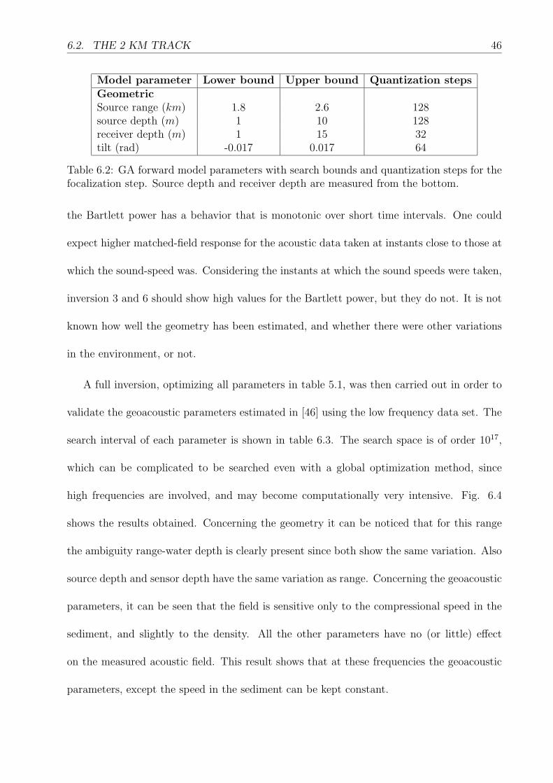
6.2. THE 2 KM TRACK 46
Model parameter Lower bound Upper bound Quantization stepsGeometricSource range (km) 1.8 2.6 128source depth (m) 1 10 128receiver depth (m) 1 15 32tilt (rad) -0.017 0.017 64
Table 6.2: GA forward model parameters with search bounds and quantization steps for thefocalization step. Source depth and receiver depth are measured from the bottom.
the Bartlett power has a behavior that is monotonic over short time intervals. One could
expect higher matched-field response for the acoustic data taken at instants close to those at
which the sound-speed was. Considering the instants at which the sound speeds were taken,
inversion 3 and 6 should show high values for the Bartlett power, but they do not. It is not
known how well the geometry has been estimated, and whether there were other variations
in the environment, or not.
A full inversion, optimizing all parameters in table 5.1, was then carried out in order to
validate the geoacoustic parameters estimated in [46] using the low frequency data set. The
search interval of each parameter is shown in table 6.3. The search space is of order 1017,
which can be complicated to be searched even with a global optimization method, since
high frequencies are involved, and may become computationally very intensive. Fig. 6.4
shows the results obtained. Concerning the geometry it can be noticed that for this range
the ambiguity range-water depth is clearly present since both show the same variation. Also
source depth and sensor depth have the same variation as range. Concerning the geoacoustic
parameters, it can be seen that the field is sensitive only to the compressional speed in the
sediment, and slightly to the density. All the other parameters have no (or little) effect
on the measured acoustic field. This result shows that at these frequencies the geoacoustic
parameters, except the speed in the sediment can be kept constant.
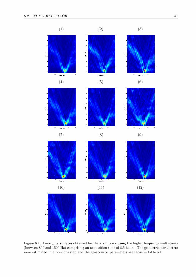
6.2. THE 2 KM TRACK 47
(1) (2) (3)
(4) (5) (6)
(7) (8) (9)
(10) (11) (12)
Figure 6.1: Ambiguity surfaces obtained for the 2 km track using the higher frequency multi-tones(between 800 and 1500 Hz) comprising an acquisition time of 8.5 hours. The geometric parameterswere estimated in a previous step and the geoacoustic parameters are those in table 5.1.
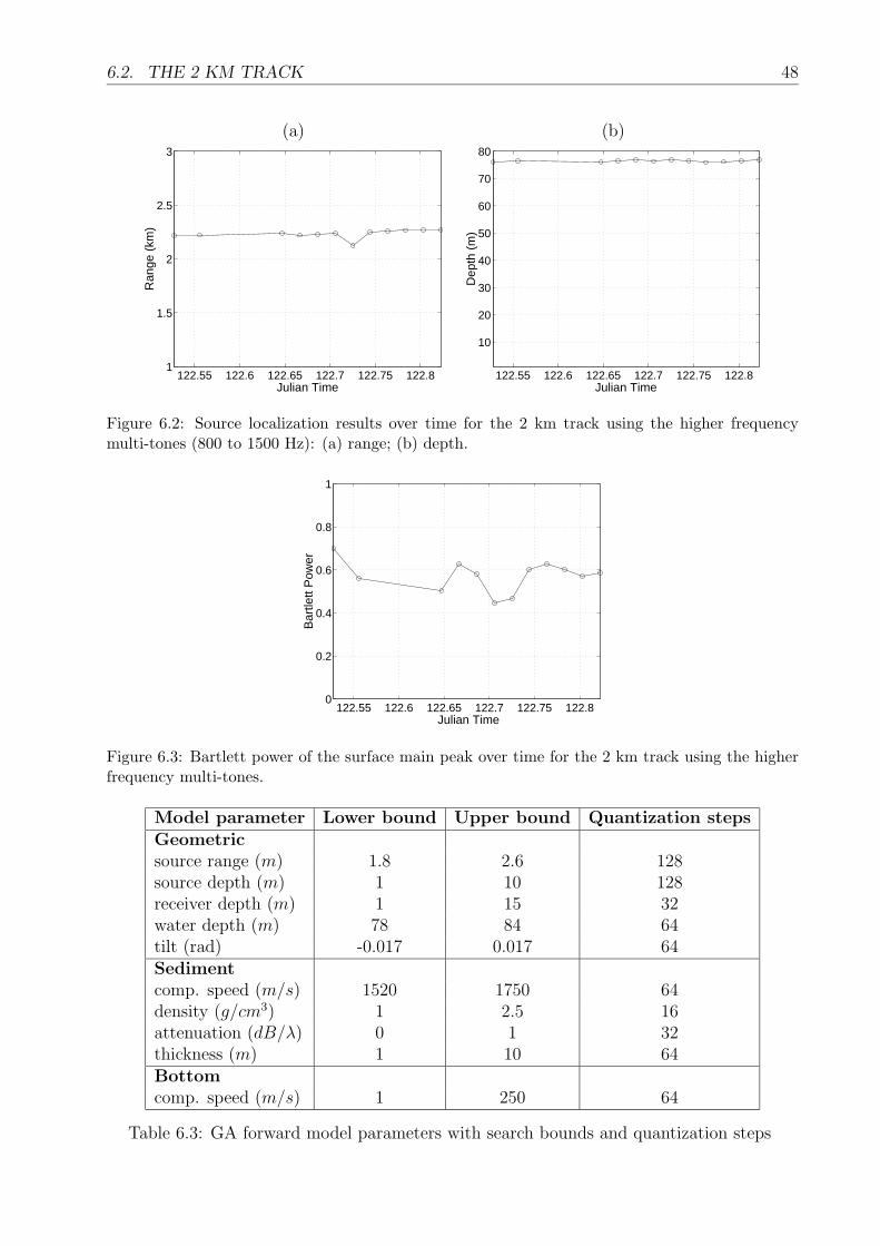
6.2. THE 2 KM TRACK 48
(a) (b)
122.55 122.6 122.65 122.7 122.75 122.81
1.5
2
2.5
3R
ange
(km
)
Julian Time122.55 122.6 122.65 122.7 122.75 122.8
10
20
30
40
50
60
70
80
Dep
th (
m)
Julian Time
Figure 6.2: Source localization results over time for the 2 km track using the higher frequencymulti-tones (800 to 1500 Hz): (a) range; (b) depth.
122.55 122.6 122.65 122.7 122.75 122.80
0.2
0.4
0.6
0.8
1
Bar
tlett
Pow
er
Julian Time
Figure 6.3: Bartlett power of the surface main peak over time for the 2 km track using the higherfrequency multi-tones.
Model parameter Lower bound Upper bound Quantization stepsGeometricsource range (m) 1.8 2.6 128source depth (m) 1 10 128receiver depth (m) 1 15 32water depth (m) 78 84 64tilt (rad) -0.017 0.017 64Sedimentcomp. speed (m/s) 1520 1750 64density (g/cm3) 1 2.5 16attenuation (dB/λ) 0 1 32thickness (m) 1 10 64Bottomcomp. speed (m/s) 1 250 64
Table 6.3: GA forward model parameters with search bounds and quantization steps
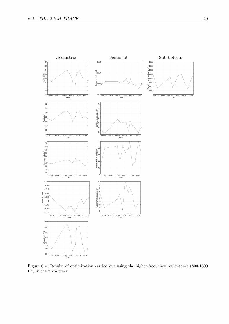
6.2. THE 2 KM TRACK 49
Geometric Sediment Sub-bottom
122.55 122.6 122.65 122.7 122.75 122.81.8
1.9
2
2.1
2.2
2.3
2.4
2.5
2.6
Time
Ran
ge (
km)
122.55 122.6 122.65 122.7 122.75 122.81500
1550
1600
1650
TimeS
peed
in s
ed. (
m/s
)122.55 122.6 122.65 122.7 122.75 122.8
1550
1600
1650
1700
1750
1800
1850
1900
Time
Spe
ed in
sub
−bo
ttom
(m
/s)
122.55 122.6 122.65 122.7 122.75 122.868
70
72
74
76
78
80
82
Time
Dep
th (
m)
122.55 122.6 122.65 122.7 122.75 122.8
1.2
1.4
1.6
1.8
2
2.2
2.4
Time
Den
sity
in s
ed. (
g/cm
3 )
122.55 122.6 122.65 122.7 122.75 122.8
64
66
68
70
72
74
76
78
80
82
Time
Sen
sord
epth
(m
)
122.55 122.6 122.65 122.7 122.75 122.80
0.2
0.4
0.6
0.8
1
Time
Atte
nuat
ion
in s
ed (
dB/λ
)
122.55 122.6 122.65 122.7 122.75 122.8
−0.015
−0.01
−0.005
0
0.005
0.01
0.015
0.02
0.025
Time
Arr
ay ti
lt (r
ad)
122.55 122.6 122.65 122.7 122.75 122.8
1
2
3
4
5
6
7
8
9
10
Time
Sed
imen
t thi
ckne
ss (
m)
122.55 122.6 122.65 122.7 122.75 122.878
79
80
81
82
83
84
Time
Wat
erde
pth
(m)
Figure 6.4: Results of optimization carried out using the higher-frequency multi-tones (800-1500Hz) in the 2 km track.
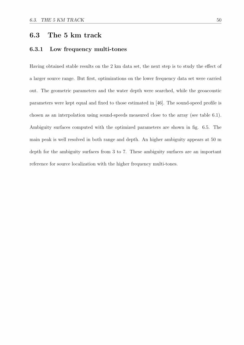
6.3. THE 5 KM TRACK 50
6.3 The 5 km track
6.3.1 Low frequency multi-tones
Having obtained stable results on the 2 km data set, the next step is to study the effect of
a larger source range. But first, optimizations on the lower frequency data set were carried
out. The geometric parameters and the water depth were searched, while the geoacoustic
parameters were kept equal and fixed to those estimated in [46]. The sound-speed profile is
chosen as an interpolation using sound-speeds measured close to the array (see table 6.1).
Ambiguity surfaces computed with the optimized parameters are shown in fig. 6.5. The
main peak is well resolved in both range and depth. An higher ambiguity appears at 50 m
depth for the ambiguity surfaces from 3 to 7. These ambiguity surfaces are an important
reference for source localization with the higher frequency multi-tones.
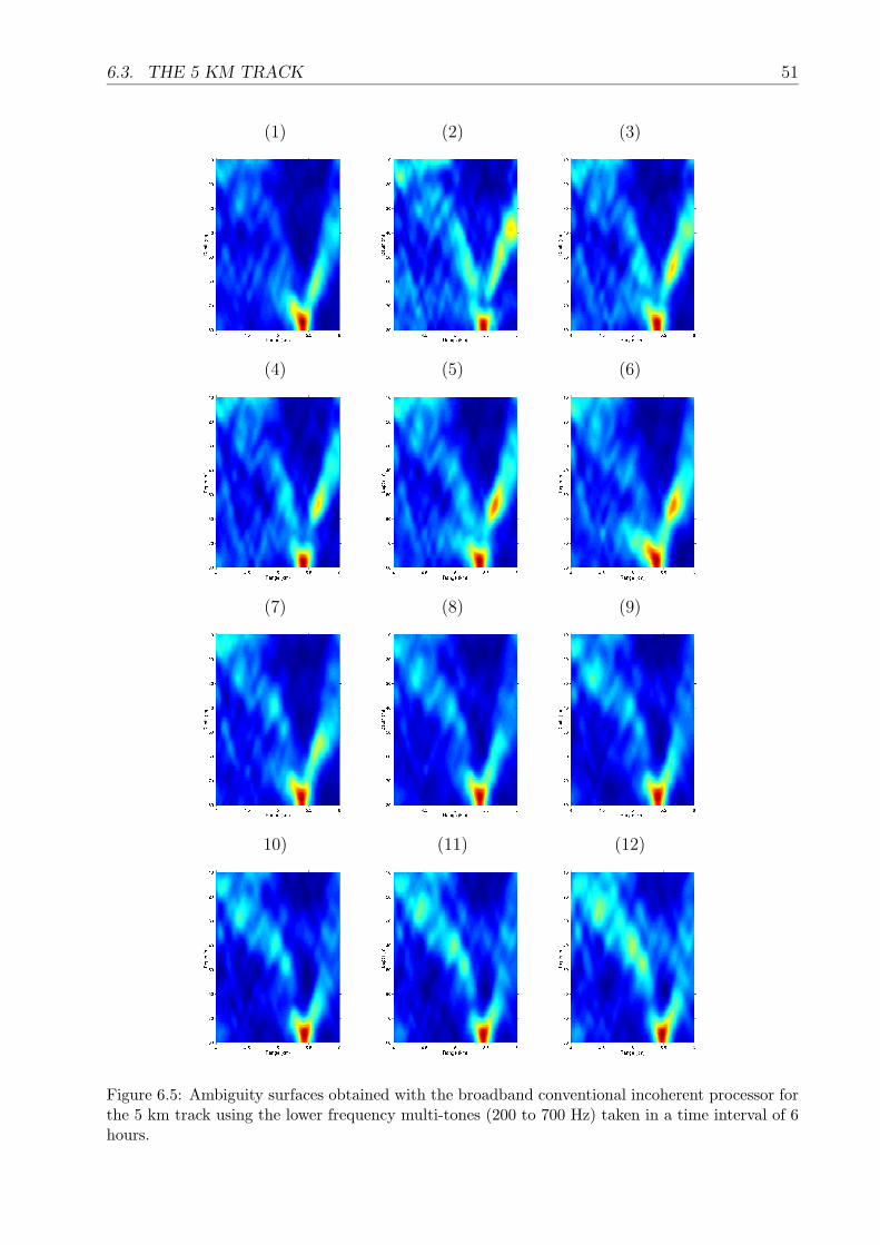
6.3. THE 5 KM TRACK 51
(1) (2) (3)
(4) (5) (6)
(7) (8) (9)
10) (11) (12)
Figure 6.5: Ambiguity surfaces obtained with the broadband conventional incoherent processor forthe 5 km track using the lower frequency multi-tones (200 to 700 Hz) taken in a time interval of 6hours.
6.3. THE 5 KM TRACK 52
6.3.2 High frequency tones: blind focalization of main parameters
The first optimizations on the 5 km acoustic data using higher frequencies were carried
out optimizing all parameters to which the acoustic field has shown to be sensitive in the
previous optimizations on the 2 km range. Those are the geometric parameters (range,
depth, array depth, array tilt), water depth, and sediment sound-speed. Every 32 minutes
a 10 seconds ping was taken giving a total of 12 pings comprising nearly 6 hours. Fig.
6.6 shows the ambiguity surfaces obtained with parameter estimates obtained in a previous
step (not shown). Significant ambiguities appear in every range-depth ambiguity surface.
There is one ambiguity that appears in the first 6 surfaces close to the 75 m depth and
between 5 and 6 km range. This gives hope regarding to an improved modeling scheme. In
surfaces 4 and 5, the maximum is present on the same location which gives some confidence
to correspond to the correct value, since they differ about 32 minutes in time. In surfaces 7
to 12 the structure that could be found in surfaces 1 to 6 completely disappears. As it can
be seen, serious problems are present for the 5 km track.
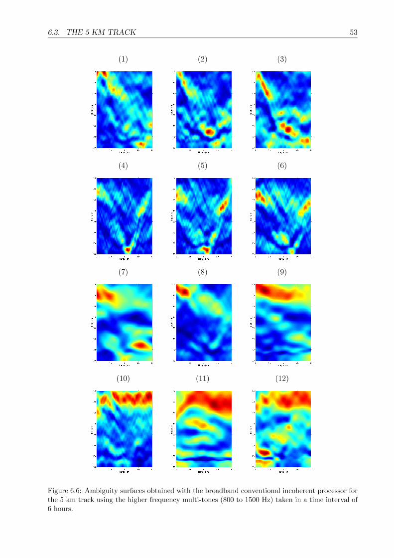
6.3. THE 5 KM TRACK 53
(1) (2) (3)
(4) (5) (6)
(7) (8) (9)
(10) (11) (12)
Figure 6.6: Ambiguity surfaces obtained with the broadband conventional incoherent processor forthe 5 km track using the higher frequency multi-tones (800 to 1500 Hz) taken in a time interval of6 hours.
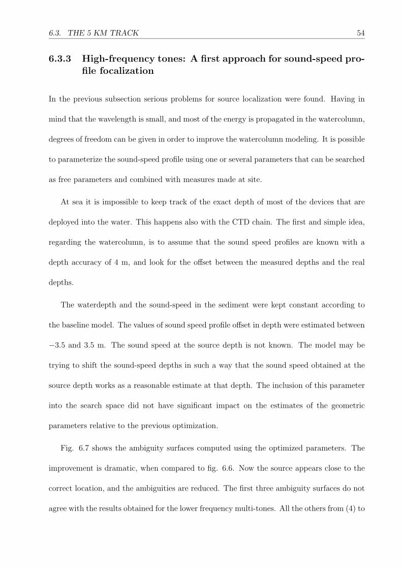
6.3. THE 5 KM TRACK 54
6.3.3 High-frequency tones: A first approach for sound-speed pro-file focalization
In the previous subsection serious problems for source localization were found. Having in
mind that the wavelength is small, and most of the energy is propagated in the watercolumn,
degrees of freedom can be given in order to improve the watercolumn modeling. It is possible
to parameterize the sound-speed profile using one or several parameters that can be searched
as free parameters and combined with measures made at site.
At sea it is impossible to keep track of the exact depth of most of the devices that are
deployed into the water. This happens also with the CTD chain. The first and simple idea,
regarding the watercolumn, is to assume that the sound speed profiles are known with a
depth accuracy of 4 m, and look for the offset between the measured depths and the real
depths.
The waterdepth and the sound-speed in the sediment were kept constant according to
the baseline model. The values of sound speed profile offset in depth were estimated between
−3.5 and 3.5 m. The sound speed at the source depth is not known. The model may be
trying to shift the sound-speed depths in such a way that the sound speed obtained at the
source depth works as a reasonable estimate at that depth. The inclusion of this parameter
into the search space did not have significant impact on the estimates of the geometric
parameters relative to the previous optimization.
Fig. 6.7 shows the ambiguity surfaces computed using the optimized parameters. The
improvement is dramatic, when compared to fig. 6.6. Now the source appears close to the
correct location, and the ambiguities are reduced. The first three ambiguity surfaces do not
agree with the results obtained for the lower frequency multi-tones. All the others from (4) to

6.3. THE 5 KM TRACK 55
(12) show similar results, having the source at 5.4 km in most of the cases. However, a strong
ambiguity structure is always present. It can be noticed that the mainlobes and sidelobes
are very large for these frequencies, and compared to those lobes in the ambiguity surfaces
obtained for the lower frequencies. The reason may be a poorly focused environment. In the
next section estimates of the sound speed at the source depth will be presented.
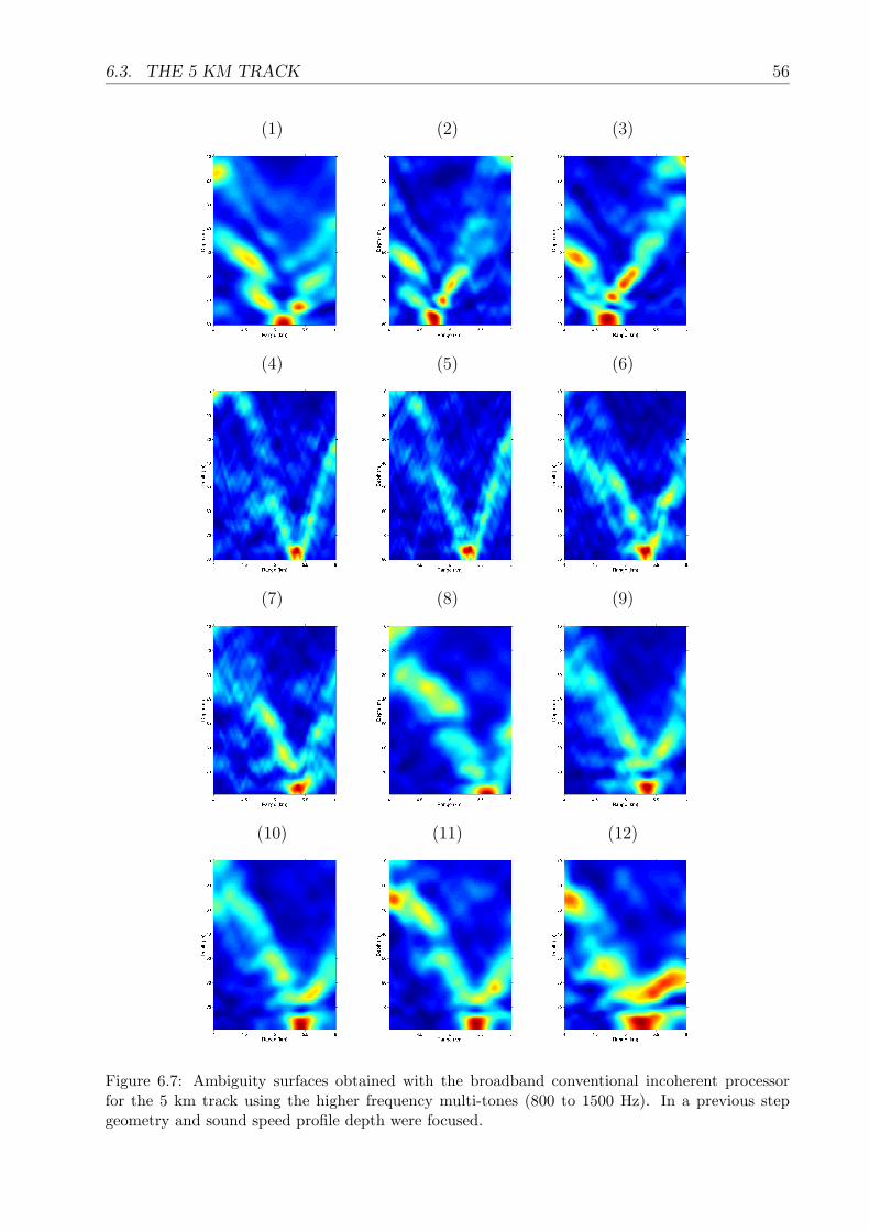
6.3. THE 5 KM TRACK 56
(1) (2) (3)
(4) (5) (6)
(7) (8) (9)
(10) (11) (12)
Figure 6.7: Ambiguity surfaces obtained with the broadband conventional incoherent processorfor the 5 km track using the higher frequency multi-tones (800 to 1500 Hz). In a previous stepgeometry and sound speed profile depth were focused.
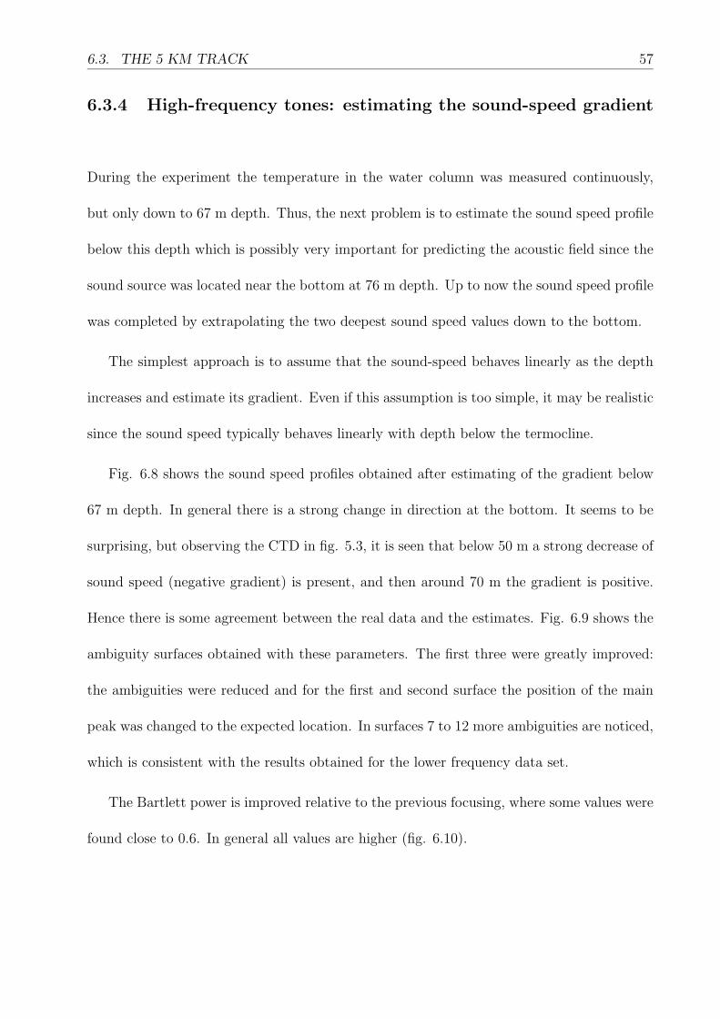
6.3. THE 5 KM TRACK 57
6.3.4 High-frequency tones: estimating the sound-speed gradient
During the experiment the temperature in the water column was measured continuously,
but only down to 67 m depth. Thus, the next problem is to estimate the sound speed profile
below this depth which is possibly very important for predicting the acoustic field since the
sound source was located near the bottom at 76 m depth. Up to now the sound speed profile
was completed by extrapolating the two deepest sound speed values down to the bottom.
The simplest approach is to assume that the sound-speed behaves linearly as the depth
increases and estimate its gradient. Even if this assumption is too simple, it may be realistic
since the sound speed typically behaves linearly with depth below the termocline.
Fig. 6.8 shows the sound speed profiles obtained after estimating of the gradient below
67 m depth. In general there is a strong change in direction at the bottom. It seems to be
surprising, but observing the CTD in fig. 5.3, it is seen that below 50 m a strong decrease of
sound speed (negative gradient) is present, and then around 70 m the gradient is positive.
Hence there is some agreement between the real data and the estimates. Fig. 6.9 shows the
ambiguity surfaces obtained with these parameters. The first three were greatly improved:
the ambiguities were reduced and for the first and second surface the position of the main
peak was changed to the expected location. In surfaces 7 to 12 more ambiguities are noticed,
which is consistent with the results obtained for the lower frequency data set.
The Bartlett power is improved relative to the previous focusing, where some values were
found close to 0.6. In general all values are higher (fig. 6.10).
6.3. THE 5 KM TRACK 58
(1) (2) (3)
1509 1510 1511 1512 1513
0
10
20
30
40
50
60
70
80
Soundspeed (m/s)
Dep
th (
m)
1509 1510 1511 1512 1513
0
10
20
30
40
50
60
70
80
Soundspeed (m/s)
Dep
th (
m)
1509 1510 1511 1512 1513
0
10
20
30
40
50
60
70
80
Soundspeed (m/s)
Dep
th (
m)
(4) (5) (6)
1509 1510 1511 1512 1513
0
10
20
30
40
50
60
70
80
Soundspeed (m/s)
Dep
th (
m)
1509 1510 1511 1512 1513
0
10
20
30
40
50
60
70
80
Soundspeed (m/s)
Dep
th (
m)
1509 1510 1511 1512 1513
0
10
20
30
40
50
60
70
80
Soundspeed (m/s)
Dep
th (
m)
(7) (8) (9)
1509 1510 1511 1512 1513
0
10
20
30
40
50
60
70
80
Soundspeed (m/s)
Dep
th (
m)
1509 1510 1511 1512 1513
0
10
20
30
40
50
60
70
80
Soundspeed (m/s)
Dep
th (
m)
1509 1510 1511 1512 1513
0
10
20
30
40
50
60
70
80
Soundspeed (m/s)
Dep
th (
m)
(10) (11) (12)
1509 1510 1511 1512 1513
0
10
20
30
40
50
60
70
80
Soundspeed (m/s)
Dep
th (
m)
1509 1510 1511 1512 1513
0
10
20
30
40
50
60
70
80
Soundspeed (m/s)
Dep
th (
m)
1509 1510 1511 1512 1513
0
10
20
30
40
50
60
70
80
Soundspeed (m/s)
Dep
th (
m)
Figure 6.8: Optimization results for sound speed gradients below 67 m depth for the 5 km trackby focalization using the higher frequency multi-tones (800 to 1500 Hz).
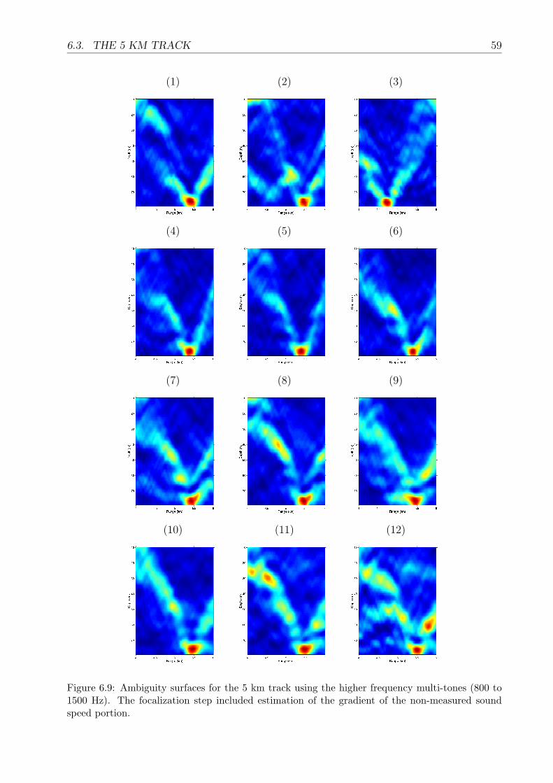
6.3. THE 5 KM TRACK 59
(1) (2) (3)
(4) (5) (6)
(7) (8) (9)
(10) (11) (12)
Figure 6.9: Ambiguity surfaces for the 5 km track using the higher frequency multi-tones (800 to1500 Hz). The focalization step included estimation of the gradient of the non-measured soundspeed portion.
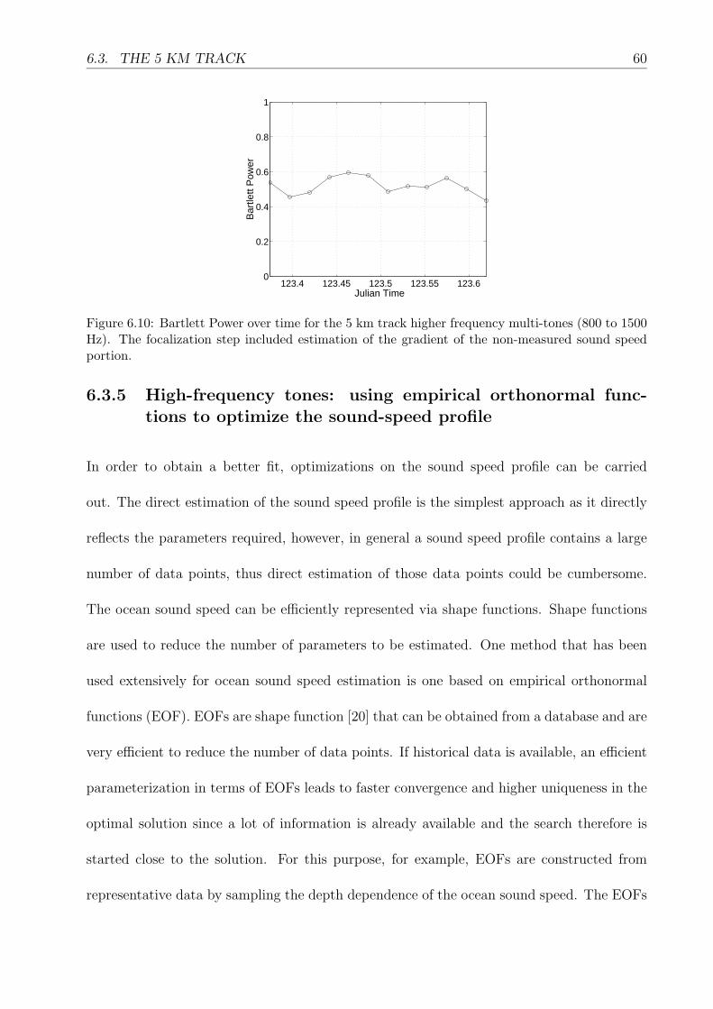
6.3. THE 5 KM TRACK 60
123.4 123.45 123.5 123.55 123.60
0.2
0.4
0.6
0.8
1
Bar
tlett
Pow
er
Julian Time
Figure 6.10: Bartlett Power over time for the 5 km track higher frequency multi-tones (800 to 1500Hz). The focalization step included estimation of the gradient of the non-measured sound speedportion.
6.3.5 High-frequency tones: using empirical orthonormal func-tions to optimize the sound-speed profile
In order to obtain a better fit, optimizations on the sound speed profile can be carried
out. The direct estimation of the sound speed profile is the simplest approach as it directly
reflects the parameters required, however, in general a sound speed profile contains a large
number of data points, thus direct estimation of those data points could be cumbersome.
The ocean sound speed can be efficiently represented via shape functions. Shape functions
are used to reduce the number of parameters to be estimated. One method that has been
used extensively for ocean sound speed estimation is one based on empirical orthonormal
functions (EOF). EOFs are shape function [20] that can be obtained from a database and are
very efficient to reduce the number of data points. If historical data is available, an efficient
parameterization in terms of EOFs leads to faster convergence and higher uniqueness in the
optimal solution since a lot of information is already available and the search therefore is
started close to the solution. For this purpose, for example, EOFs are constructed from
representative data by sampling the depth dependence of the ocean sound speed. The EOFs
6.3. THE 5 KM TRACK 61
are obtained by using singular value decomposition (SVD) of a matrix C with columns
Ci = ci − c, (6.1)
where ci are the real profiles available, and c is the average profile. The SVD is known to be
C = UDV, (6.2)
where D is a diagonal matrix with the singular values, and U is a matrix with orthogonal
columns, which are used as the EOFs. The sound-speed profile is obtained by
CEOF = c+N∑n=1
αnUn, (6.3)
where N is the number of EOFs to be combined, which is selected by observation of the
singular values by using some empirical criteria. Experimental results have shown that
usually the 2 or 3 first EOFs are enough to achieve a high degree of accuracy. The use of
EOFs involves historical data that in the case of the water column sound speed profile can
be acquired over time and space. Thus, one can expect to have sufficient information to
enable the model to obtain a profile that best represents the watercolumn over range, depth
and time.
EOFs were used to improve the environmental focalization and hence the source local-
ization results obtained up to now. The criteria used to select the number of relevant EOFs
for the available data was
N = minN∑Nn=1 λ
2n∑M
m=1 λ2m
> 0.8 (6.4)
where the λn are the singular values obtained by the SVD, M is the total number of singular
values, provided that λ1 ≥ λ2 ≥ . . . ≥ λM . For this data set the criteria (6.4) yielded N =
3, i.e. the first three EOFs are sufficient to model the sound speed with enough accuracy.
6.3. THE 5 KM TRACK 62
The coefficients αn, which are the coefficients of the linear combination of EOFs, are now
part of the search space, i.e., they are searched as free parameters, such as the geometry and
the other parameters concerning the sound speed. By trial and error, the search interval
for these coefficients was set between -5 and 5. Fig. 6.11 shows comparisons between the
sound speed profiles obtained by interpolation and those obtained through the combination
of the EOFs. It can be seen that some are closely matched, but other differ over the
whole watercolumn. This depends on how range or time dependent the sound speed was
through the sea trial, or it was simply the sound-speed through which the best match between
replicas and real data could be obtained. Observing the ambiguity surfaces obtained with the
estimated sound-speed profiles (fig. 6.11), it can be seen that the main peak is always nearly
at the same location, with negligible variations, and the ambiguities could be suppressed
(fig. 6.12). Finally the plots shown in figs. 6.13 and 6.14 respectively summarize the
localizations and Bartlett power obtained over time. The estimation of the sound speed by
EOFs improved significantly the Bartlett power values relative to those obtained in section
6.3.4.
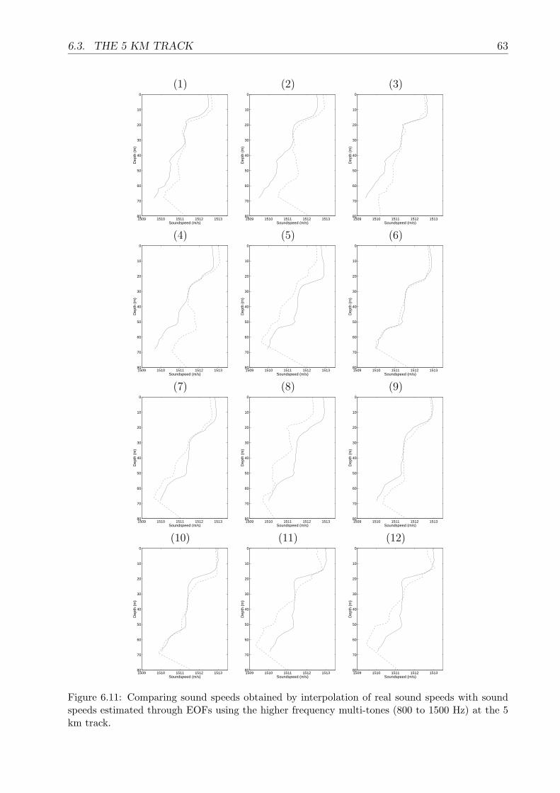
6.3. THE 5 KM TRACK 63
(1) (2) (3)
1509 1510 1511 1512 1513
0
10
20
30
40
50
60
70
80
Soundspeed (m/s)
Dep
th (
m)
1509 1510 1511 1512 1513
0
10
20
30
40
50
60
70
80
Soundspeed (m/s)
Dep
th (
m)
1509 1510 1511 1512 1513
0
10
20
30
40
50
60
70
80
Soundspeed (m/s)
Dep
th (
m)
(4) (5) (6)
1509 1510 1511 1512 1513
0
10
20
30
40
50
60
70
80
Soundspeed (m/s)
Dep
th (
m)
1509 1510 1511 1512 1513
0
10
20
30
40
50
60
70
80
Soundspeed (m/s)
Dep
th (
m)
1509 1510 1511 1512 1513
0
10
20
30
40
50
60
70
80
Soundspeed (m/s)
Dep
th (
m)
(7) (8) (9)
1509 1510 1511 1512 1513
0
10
20
30
40
50
60
70
80
Soundspeed (m/s)
Dep
th (
m)
1509 1510 1511 1512 1513
0
10
20
30
40
50
60
70
80
Soundspeed (m/s)
Dep
th (
m)
1509 1510 1511 1512 1513
0
10
20
30
40
50
60
70
80
Soundspeed (m/s)
Dep
th (
m)
(10) (11) (12)
1509 1510 1511 1512 1513
0
10
20
30
40
50
60
70
80
Soundspeed (m/s)
Dep
th (
m)
1509 1510 1511 1512 1513
0
10
20
30
40
50
60
70
80
Soundspeed (m/s)
Dep
th (
m)
1509 1510 1511 1512 1513
0
10
20
30
40
50
60
70
80
Soundspeed (m/s)
Dep
th (
m)
Figure 6.11: Comparing sound speeds obtained by interpolation of real sound speeds with soundspeeds estimated through EOFs using the higher frequency multi-tones (800 to 1500 Hz) at the 5km track.
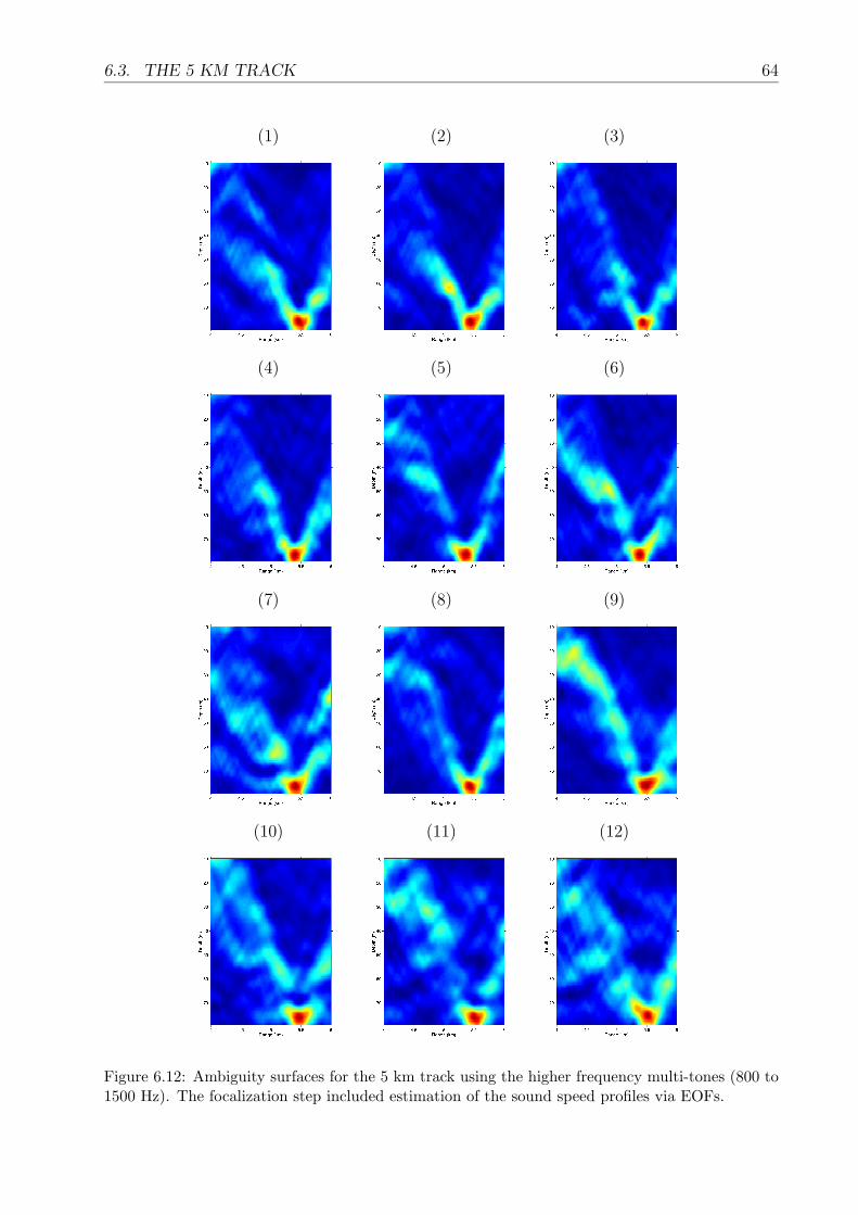
6.3. THE 5 KM TRACK 64
(1) (2) (3)
(4) (5) (6)
(7) (8) (9)
(10) (11) (12)
Figure 6.12: Ambiguity surfaces for the 5 km track using the higher frequency multi-tones (800 to1500 Hz). The focalization step included estimation of the sound speed profiles via EOFs.
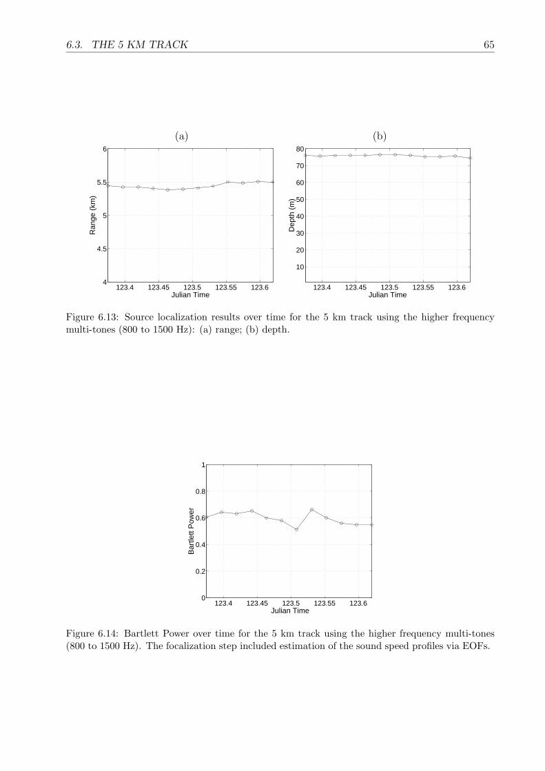
6.3. THE 5 KM TRACK 65
(a) (b)
123.4 123.45 123.5 123.55 123.64
4.5
5
5.5
6
Ran
ge (
km)
Julian Time123.4 123.45 123.5 123.55 123.6
10
20
30
40
50
60
70
80
Dep
th (
m)
Julian Time
Figure 6.13: Source localization results over time for the 5 km track using the higher frequencymulti-tones (800 to 1500 Hz): (a) range; (b) depth.
123.4 123.45 123.5 123.55 123.60
0.2
0.4
0.6
0.8
1
Bar
tlett
Pow
er
Julian Time
Figure 6.14: Bartlett Power over time for the 5 km track using the higher frequency multi-tones(800 to 1500 Hz). The focalization step included estimation of the sound speed profiles via EOFs.
6.4. THE 10 KM TRACK 66
6.4 The 10 km track
The strategy for environmental focalization followed in section 6.3 has shown to be effective
for the 5 km track, i.e., the model has shown to be matched with the reality in terms of
acoustic field. It was also shown that the modeling scheme applied at 2 km fails to accurately
localize the source at 5 km for the higher frequency data. Now the question is whether the
focusing method applied at 5 km works also at 10 km.
The sound speed profiles available were all taken along the 10 km track (see fig. 5.1). In
order to obtain the EOFs, a database of sound speed profiles was constructed with profiles
updated every 5 minutes and comprising the whole 10 km track acquisition period. By
applicating criteria (6.4) it was found that 3 EOFs were enough to represent the temperature
field.
As it was done for the 5 km track, one data ping acquired each 32 minutes comprising a
period of almost 6 hours were taken. First focalization and source localization with the lower
frequency multi-tones was carried out in order to obtain a reference. At 10 km range, it was
supposed to be likely to have some variations in water depth along the transmission track.
Thus, during focalization, water depth was included in the search space to assure that the
correct values for this parameter is used in the source localization step. Fig. 6.15 shows plots
with estimates of source range and waterdepth over time for the lower frequency multi-tones.
The ambiguity between source range and water depth is clearly present, as it can be seen by
observing the shape of the curves. Taking fig. 3.7 (a) as an example it can be seen that for a
continuous set of source range and water depth a matched-field response close to maximum
is obtained (note that this is noise free simulated data). If noise or a mismatch situation
occurs, then the maximum of the objective function may change to another location on the
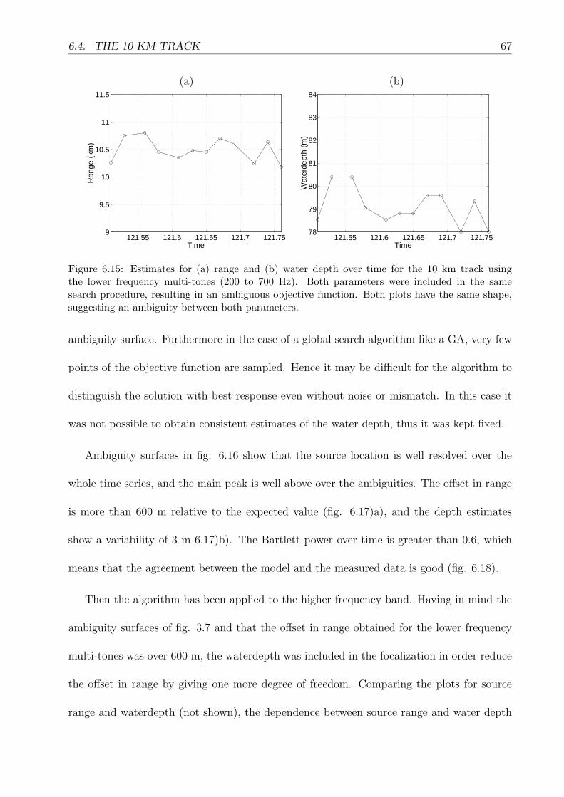
6.4. THE 10 KM TRACK 67
(a) (b)
121.55 121.6 121.65 121.7 121.759
9.5
10
10.5
11
11.5
Time
Ran
ge (
km)
121.55 121.6 121.65 121.7 121.7578
79
80
81
82
83
84
Time
Wat
erde
pth
(m)
Figure 6.15: Estimates for (a) range and (b) water depth over time for the 10 km track usingthe lower frequency multi-tones (200 to 700 Hz). Both parameters were included in the samesearch procedure, resulting in an ambiguous objective function. Both plots have the same shape,suggesting an ambiguity between both parameters.
ambiguity surface. Furthermore in the case of a global search algorithm like a GA, very few
points of the objective function are sampled. Hence it may be difficult for the algorithm to
distinguish the solution with best response even without noise or mismatch. In this case it
was not possible to obtain consistent estimates of the water depth, thus it was kept fixed.
Ambiguity surfaces in fig. 6.16 show that the source location is well resolved over the
whole time series, and the main peak is well above over the ambiguities. The offset in range
is more than 600 m relative to the expected value (fig. 6.17)a), and the depth estimates
show a variability of 3 m 6.17)b). The Bartlett power over time is greater than 0.6, which
means that the agreement between the model and the measured data is good (fig. 6.18).
Then the algorithm has been applied to the higher frequency band. Having in mind the
ambiguity surfaces of fig. 3.7 and that the offset in range obtained for the lower frequency
multi-tones was over 600 m, the waterdepth was included in the focalization in order reduce
the offset in range by giving one more degree of freedom. Comparing the plots for source
range and waterdepth (not shown), the dependence between source range and water depth
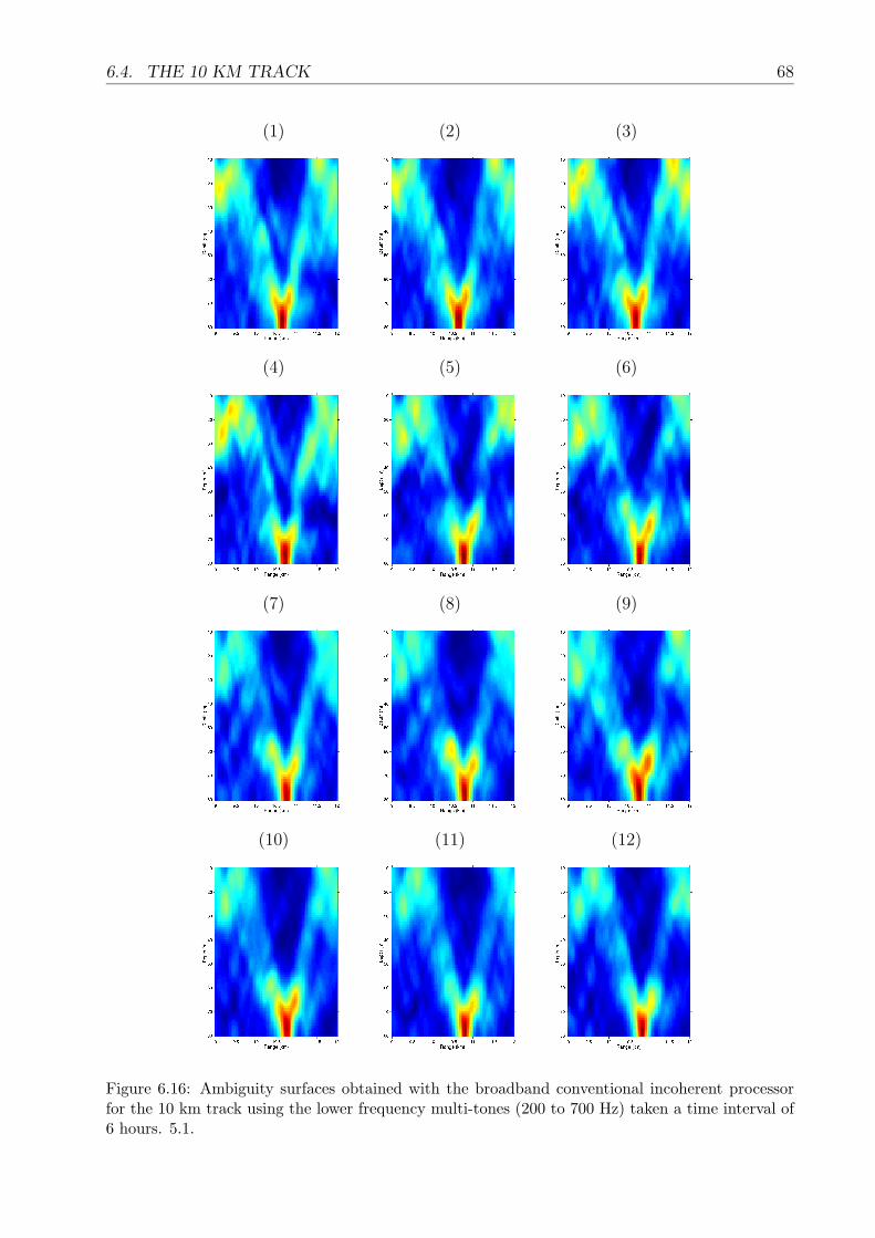
6.4. THE 10 KM TRACK 68
(1) (2) (3)
(4) (5) (6)
(7) (8) (9)
(10) (11) (12)
Figure 6.16: Ambiguity surfaces obtained with the broadband conventional incoherent processorfor the 10 km track using the lower frequency multi-tones (200 to 700 Hz) taken a time interval of6 hours. 5.1.
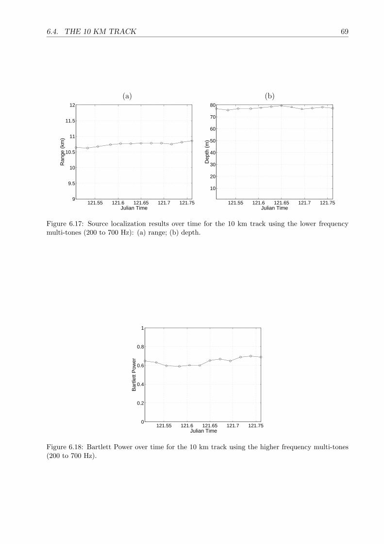
6.4. THE 10 KM TRACK 69
(a) (b)
121.55 121.6 121.65 121.7 121.759
9.5
10
10.5
11
11.5
12
Ran
ge (
km)
Julian Time121.55 121.6 121.65 121.7 121.75
10
20
30
40
50
60
70
80
Dep
th (
m)
Julian Time
Figure 6.17: Source localization results over time for the 10 km track using the lower frequencymulti-tones (200 to 700 Hz): (a) range; (b) depth.
121.55 121.6 121.65 121.7 121.750
0.2
0.4
0.6
0.8
1
Bar
tlett
Pow
er
Julian Time
Figure 6.18: Bartlett Power over time for the 10 km track using the higher frequency multi-tones(200 to 700 Hz).
6.4. THE 10 KM TRACK 70
is not noticed anymore, which is in agreement with the example in figure 3.7. The ambiguity
surfaces obtained for the data pings analyzed are shown in fig. 6.19. It can be noticed that
the main peak is not completely stable in its correct position, but it always appears close to
the correct location. Range varies between 10 and 11 km (fig. 6.20a)), and the depth has a
variability between 71 and 77 m (fig. 6.20b)). The Bartlett power is low, ranging from 0.3
to 0.5 (fig. 6.21), but the main peak was not overtaken by the sidelobes.
The source localization experimental results obtained for the multi-tones are satisfactory.
However, considerable variation both in range and in depth is noticed. These tones comprised
6 frequencies ranging from 800 to 1500 Hz. The issue is to know whether the modeling
has reached its limitations, or whether it is possible to increase the amount of information
inserted in the localization process by using more frequencies. Experimental results have
shown that more frequencies may result in more consistent localization results [47]. Thus
the linear frequency modulated (LFM) signals collected during the sea trial were used in
order to increase the number of frequencies to better focus the environment and the source
location. A number of 15 frequencies ranging from 820 to 1500 Hz with a spacing of 23.4 Hz
were used. However, only one signal realization was used in the averaging of the covariance
matrices. Observing the ambiguity surfaces obtained (see fig. 6.22), and comparing with
those obtained for the multi-tones 6.19, no obvious improvement has been obtained relative
to sidelobe reduction. However fig. 6.23 shows that the variability in range over the whole
estimation time has been reduced from 1 to 0.3 km if pings 6 and 12 are excluded. The
depth has two outliers, but for the other estimates the variability is approximately the same
as that obtain with tones. The Bartlett power is lower than for the multi-tones (fig. 6.24),
and therefore model-data mismatch is higher in the best match situation.

6.4. THE 10 KM TRACK 71
(1) (2) (3)
(4) (5) (6)
(7) (8) (9)
(10) (11) (12)
Figure 6.19: Ambiguity surfaces obtained with the broadband conventional incoherent processorfor the 10 km track using the higher frequency multi-tones (800 to 1500 Hz).

6.4. THE 10 KM TRACK 72
(a) (b)
121.55 121.6 121.65 121.7 121.759
9.5
10
10.5
11
11.5
12
Ran
ge (
km)
Julian Time121.55 121.6 121.65 121.7 121.75
10
20
30
40
50
60
70
80
Dep
th (
m)
Julian Time
Figure 6.20: Source localization results over time for the 10 km track using the higher frequencymulti-tones (800 to 1500 Hz): (a) range; (b) depth.
121.55 121.6 121.65 121.7 121.750
0.2
0.4
0.6
0.8
1
Bar
tlett
Pow
er
Julian Time
Figure 6.21: Bartlett Power over time for the 10 km track using the higher frequency multi-tones(800 to 1500 Hz).
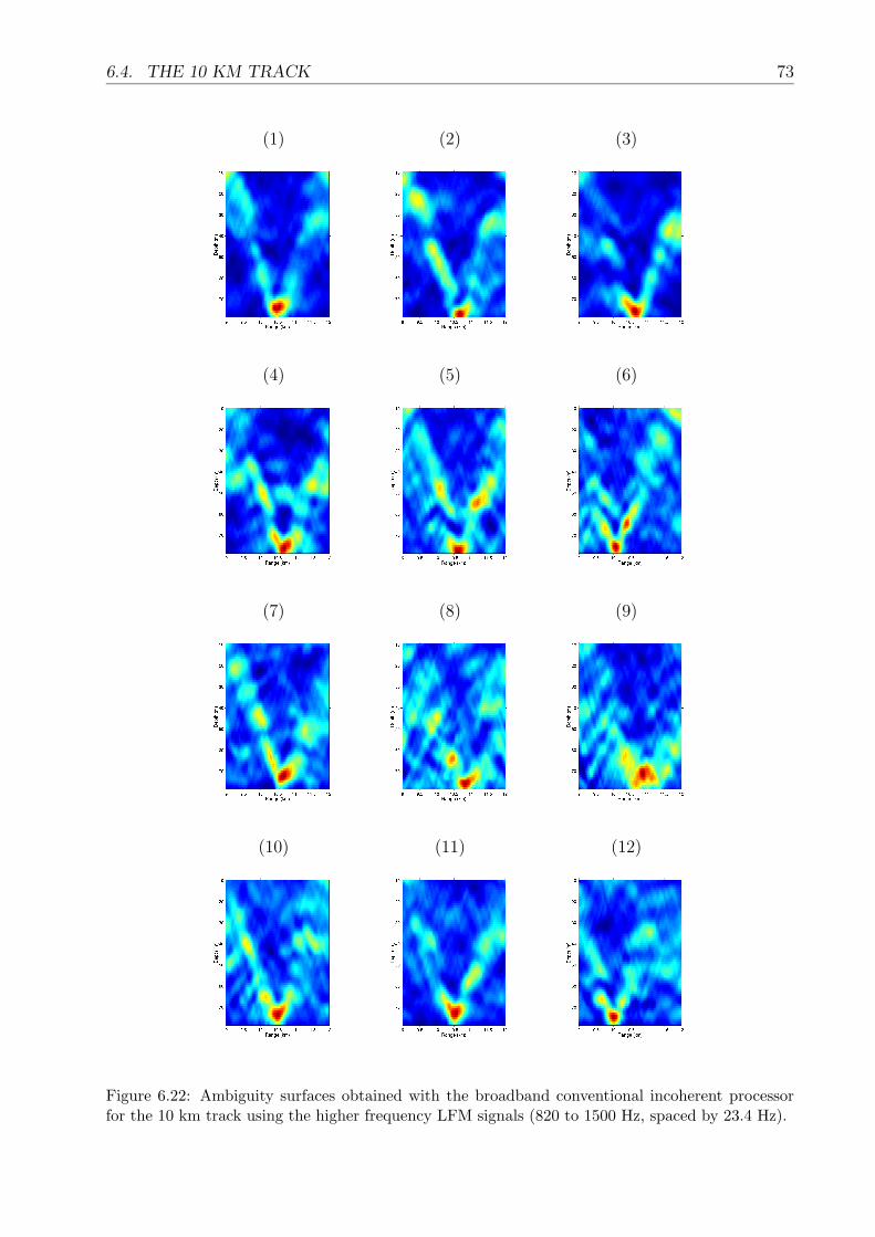
6.4. THE 10 KM TRACK 73
(1) (2) (3)
(4) (5) (6)
(7) (8) (9)
(10) (11) (12)
Figure 6.22: Ambiguity surfaces obtained with the broadband conventional incoherent processorfor the 10 km track using the higher frequency LFM signals (820 to 1500 Hz, spaced by 23.4 Hz).
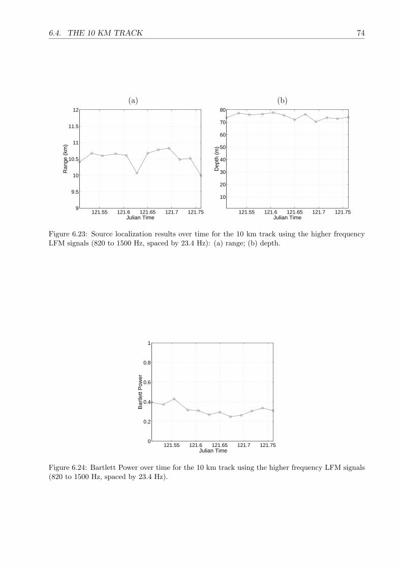
6.4. THE 10 KM TRACK 74
(a) (b)
121.55 121.6 121.65 121.7 121.759
9.5
10
10.5
11
11.5
12
Ran
ge (
km)
Julian Time121.55 121.6 121.65 121.7 121.75
10
20
30
40
50
60
70
80
Dep
th (
m)
Julian Time
Figure 6.23: Source localization results over time for the 10 km track using the higher frequencyLFM signals (820 to 1500 Hz, spaced by 23.4 Hz): (a) range; (b) depth.
121.55 121.6 121.65 121.7 121.750
0.2
0.4
0.6
0.8
1
Bar
tlett
Pow
er
Julian Time
Figure 6.24: Bartlett Power over time for the 10 km track using the higher frequency LFM signals(820 to 1500 Hz, spaced by 23.4 Hz).
6.5. THE 5 KM TRACK: SHRINKING THE ARRAY APERTURE 75
6.5 The 5 km track: Shrinking the array aperture
After working with an array spanning around three quarters of the watercolumn, and hav-
ing obtained good quality results at three different ranges, the goal now is to study the
dependency of the MFP procedure on the array aperture. As it is known, as the aperture is
decreased less spatial discrimination is obtained, hence resulting in higher sidelobes relative
to the main peak. In other words, and in the case of a vertical array, if the array aperture
is low the acoustic field being seen by the array is nearly a planewave. Although the main
peak-to-sidelobe ratio decreases with the array aperture, the main peak will theoretically
always be at the correct position. However, in the case of real data, geometric and environ-
mental mismatch is always present and the acoustic field is observed during a limited time.
Thus it is expected that from a certain point the reduction of the array aperture will force
the MFP procedure to fail to localize the source.
Reduced array aperture MFP was applied only to the 5 km track data, since for this
range good results with the full array were available, and could be used as reference.
The first idea was to check how long the MFP procedure would be able to yield reasonable
localization results for the 5 km track using the higher frequency multi-tones as the array
aperture was decreased. The array configuration used up to now had 31 elements spaced by
2 m. The procedure to shorten the array aperture is to leave out sensors from the top and
the bottom in such a way that the array is always centered in the watercolumn, keeping the
same spacing between sensors. The environment and geometry used were those obtained in
the last focalization step for this range, hence search being carried out only for range and
depth.
Figure 6.25 shows the results obtained by reducing the array aperture by successive
6.5. THE 5 KM TRACK: SHRINKING THE ARRAY APERTURE 76
factors of 2, i.e., from the full 31 sensors to 16, then 8 and finally to 4 sensors. The black
curve shows the result obtained previously with the full aperture. Comparing the curves
for range and depth obtained with half aperture (blue) to those obtained with full aperture,
only negligible difference is noticed. For 8 sensors (14 m of array aperture) it is still possible
to obtain reasonable source localization results (red curves). Excluding the outliers in pings
1, 2, 7 and 10, the localization results obtained, both in range and depth are the same
as previously. The 4 sensors aperture (6 m) represents a sampling of about 8% of the
watercolumn. The degradation of the results by reducing the aperture to 4 sensors (green) is
evident in fig. 6.25. Notice that the Bartlett power is highest for the 4 sensor configuration
over the whole time even if the MFP procedure failed. The increment of the Bartlett power
has been noticed since the aperture started to be reduced due to reduced complexity of the
acoustic field seen by the array. The matched-field response is a measure of the similarity
of the real acoustic field with the replicas produced by the numerical propagation model fed
with different source locations. If the aperture is less, then the uniqueness of the acoustic
field along the portion of watercolumn spanned by the field is lower, hence the match is
higher.
There is the possibility of compensating the lack of aperture by the addition of a large
number of frequencies. Taking the LFM signals, a continuous set of frequencies is available.
30 equally spaced frequencies between 800 and 1500 Hz were taken. This allowed more
ambiguity surface averaging. Fig. 6.27 shows the improvement obtained. There are still 3
outliers and some variability, but now it is possible to guess that 5.4 or 5.5 km may be the
correct value for range. This case shows that it was possible to partially compensate the
lack of information obtained by spatial sampling by increasing the number of frequencies.
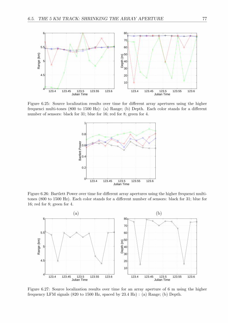
6.5. THE 5 KM TRACK: SHRINKING THE ARRAY APERTURE 77
123.4 123.45 123.5 123.55 123.64
4.5
5
5.5
6
Ran
ge (
km)
Julian Time123.4 123.45 123.5 123.55 123.6
10
20
30
40
50
60
70
80
Dep
th (
m)
Julian Time
Figure 6.25: Source localization results over time for different array apertures using the higherfrequenci multi-tones (800 to 1500 Hz): (a) Range; (b) Depth. Each color stands for a differentnumber of sensors: black for 31; blue for 16; red for 8; green for 4.
123.4 123.45 123.5 123.55 123.60
0.2
0.4
0.6
0.8
1
Bar
tlett
Pow
er
Julian Time
Figure 6.26: Bartlett Power over time for different array apertures using the higher frequenci multi-tones (800 to 1500 Hz). Each color stands for a different number of sensors: black for 31; blue for16; red for 8; green for 4.
(a) (b)
123.4 123.45 123.5 123.55 123.64
4.5
5
5.5
6
Ran
ge (
km)
Julian Time123.4 123.45 123.5 123.55 123.6
10
20
30
40
50
60
70
80
Dep
th (
m)
Julian Time
Figure 6.27: Source localization results over time for an array aperture of 6 m using the higherfrequency LFM signals (820 to 1500 Hz, spaced by 23.4 Hz) : (a) Range; (b) Depth.
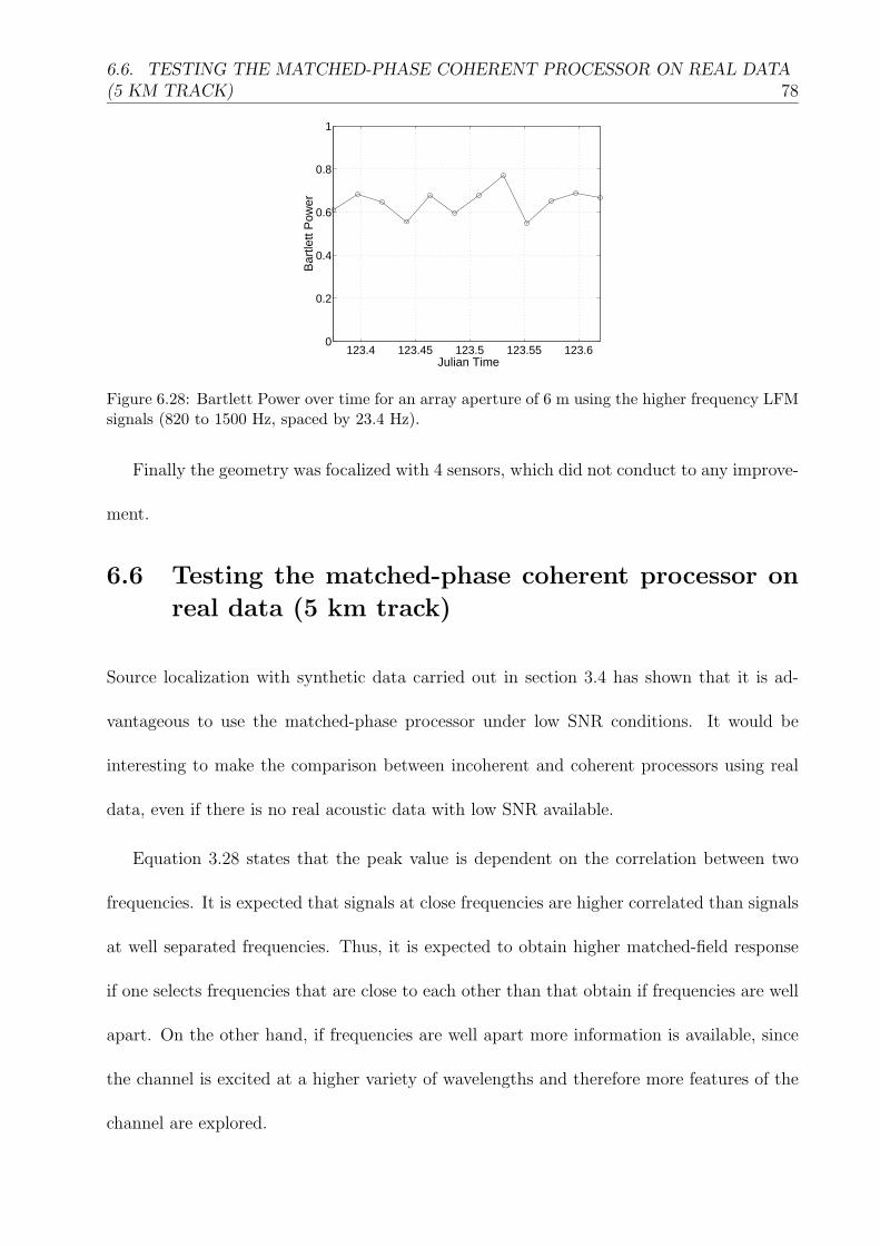
6.6. TESTING THE MATCHED-PHASE COHERENT PROCESSOR ON REAL DATA(5 KM TRACK) 78
123.4 123.45 123.5 123.55 123.60
0.2
0.4
0.6
0.8
1
Bar
tlett
Pow
er
Julian Time
Figure 6.28: Bartlett Power over time for an array aperture of 6 m using the higher frequency LFMsignals (820 to 1500 Hz, spaced by 23.4 Hz).
Finally the geometry was focalized with 4 sensors, which did not conduct to any improve-
ment.
6.6 Testing the matched-phase coherent processor on
real data (5 km track)
Source localization with synthetic data carried out in section 3.4 has shown that it is ad-
vantageous to use the matched-phase processor under low SNR conditions. It would be
interesting to make the comparison between incoherent and coherent processors using real
data, even if there is no real acoustic data with low SNR available.
Equation 3.28 states that the peak value is dependent on the correlation between two
frequencies. It is expected that signals at close frequencies are higher correlated than signals
at well separated frequencies. Thus, it is expected to obtain higher matched-field response
if one selects frequencies that are close to each other than that obtain if frequencies are well
apart. On the other hand, if frequencies are well apart more information is available, since
the channel is excited at a higher variety of wavelengths and therefore more features of the
channel are explored.
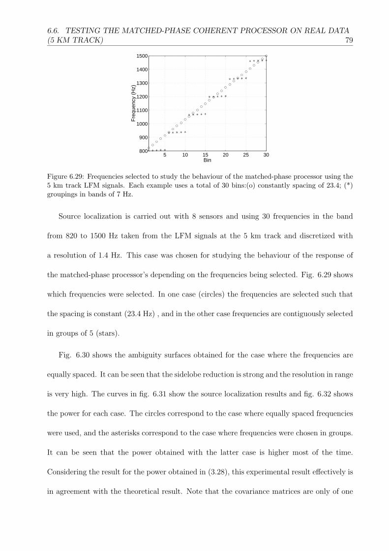
6.6. TESTING THE MATCHED-PHASE COHERENT PROCESSOR ON REAL DATA(5 KM TRACK) 79
5 10 15 20 25 30800
900
1000
1100
1200
1300
1400
1500
Bin
Fre
quen
cy (
Hz)
Figure 6.29: Frequencies selected to study the behaviour of the matched-phase processor using the5 km track LFM signals. Each example uses a total of 30 bins:(o) constantly spacing of 23.4; (*)groupings in bands of 7 Hz.
Source localization is carried out with 8 sensors and using 30 frequencies in the band
from 820 to 1500 Hz taken from the LFM signals at the 5 km track and discretized with
a resolution of 1.4 Hz. This case was chosen for studying the behaviour of the response of
the matched-phase processor’s depending on the frequencies being selected. Fig. 6.29 shows
which frequencies were selected. In one case (circles) the frequencies are selected such that
the spacing is constant (23.4 Hz) , and in the other case frequencies are contiguously selected
in groups of 5 (stars).
Fig. 6.30 shows the ambiguity surfaces obtained for the case where the frequencies are
equally spaced. It can be seen that the sidelobe reduction is strong and the resolution in range
is very high. The curves in fig. 6.31 show the source localization results and fig. 6.32 shows
the power for each case. The circles correspond to the case where equally spaced frequencies
were used, and the asterisks correspond to the case where frequencies were chosen in groups.
It can be seen that the power obtained with the latter case is higher most of the time.
Considering the result for the power obtained in (3.28), this experimental result effectively is
in agreement with the theoretical result. Note that the covariance matrices are only of one

6.6. TESTING THE MATCHED-PHASE COHERENT PROCESSOR ON REAL DATA(5 KM TRACK) 80
signal realization, therefore the variance of the estimator is high and the power estimates
may be not always accurate enough to obtain a fair comparison.
Altough the case using groups of frequencies yields higher results, the source localization
results for the case with equally spaced frequencies resulted in better source loalization, which
may be related to the higher amount of information available if frequencies are selected well
apart, as referenced at the beginning of this section.
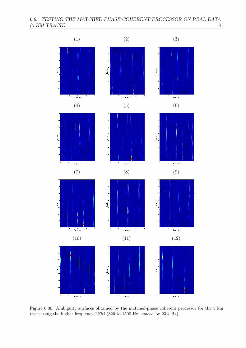
6.6. TESTING THE MATCHED-PHASE COHERENT PROCESSOR ON REAL DATA(5 KM TRACK) 81
(1) (2) (3)
(4) (5) (6)
(7) (8) (9)
(10) (11) (12)
Figure 6.30: Ambiguity surfaces obtained by the matched-phase coherent processor for the 5 kmtrack using the higher frequency LFM (820 to 1500 Hz, spaced by 23.4 Hz).
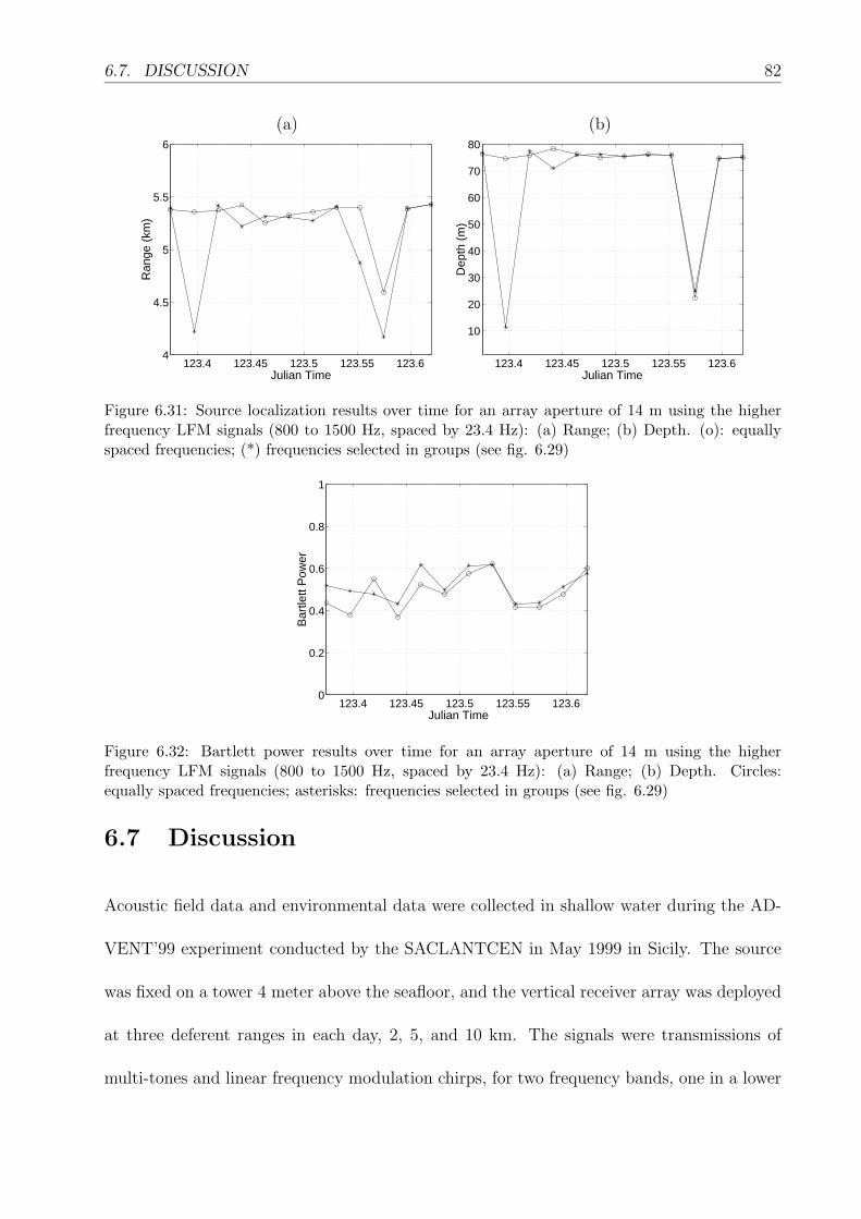
6.7. DISCUSSION 82
(a) (b)
123.4 123.45 123.5 123.55 123.64
4.5
5
5.5
6R
ange
(km
)
Julian Time123.4 123.45 123.5 123.55 123.6
10
20
30
40
50
60
70
80
Dep
th (
m)
Julian Time
Figure 6.31: Source localization results over time for an array aperture of 14 m using the higherfrequency LFM signals (800 to 1500 Hz, spaced by 23.4 Hz): (a) Range; (b) Depth. (o): equallyspaced frequencies; (*) frequencies selected in groups (see fig. 6.29)
123.4 123.45 123.5 123.55 123.60
0.2
0.4
0.6
0.8
1
Bar
tlett
Pow
er
Julian Time
Figure 6.32: Bartlett power results over time for an array aperture of 14 m using the higherfrequency LFM signals (800 to 1500 Hz, spaced by 23.4 Hz): (a) Range; (b) Depth. Circles:equally spaced frequencies; asterisks: frequencies selected in groups (see fig. 6.29)
6.7 Discussion
Acoustic field data and environmental data were collected in shallow water during the AD-
VENT’99 experiment conducted by the SACLANTCEN in May 1999 in Sicily. The source
was fixed on a tower 4 meter above the seafloor, and the vertical receiver array was deployed
at three deferent ranges in each day, 2, 5, and 10 km. The signals were transmissions of
multi-tones and linear frequency modulation chirps, for two frequency bands, one in a lower

6.7. DISCUSSION 83
frequency band (200-700 Hz), another in a higher frequency band (800-1600 Hz).
First, unknown environmental or geometric parameters were focused using a genetic
algorithm and using reduced search intervals for the location. Then, ambiguity surfaces
were computed for source localization. Algorithms were first applied to lower frequency data
to obtain reference results. This is the procedure in general steps.
For the 2 km track geoacoustic parameters estimated in a previous work with low fre-
quency data sets were used and only the geometry (tilt, receiver depth) were estimated. This
was applied only to the higher frequency multi-tones. Results are consistent and stable. Af-
terwards, a full inversion for the whole geoacoustic parameter set was carried out, and the
results have shown that the only seafloor parameter that significantly contributed for the
acoustic field was the sediment sound-speed.
The same algorithm was then applied to the 5 km track and allowed for perfectly stable
results for the lower frequency data, but failed completely to localize the source for the higher
frequency data. This is a direct consequence of the increase of the range. A larger range
implies a higher number of parameters and their possible variability over time and space.
Since the wavelength is low (between 1 and 2 m) it is likely that most of the energy
reaching the receivers is propagated through paths that have only few contacts with the
boundaries or none at all, while the other are completely absorbed by the sediment. Thus,
it is important to have a good knowledge about the water column.
Concerning the estimation of parameters in the water column, first it was assumed that
the sound-speed depths were not accurate, thus a parameter representing a shift of the
whole sound-speed was included. Estimating the uncertainty in sound-speed depths available
gave a dramatic improvement: there was clearly a repetition of the structure shown by the
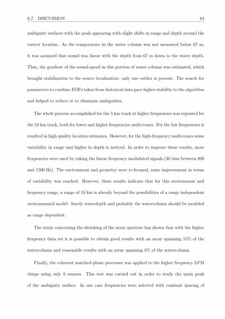
6.7. DISCUSSION 84
ambiguity surfaces with the peak appearing with slight shifts in range and depth around the
correct location. As the temperature in the water column was not measured below 67 m,
it was assumed that sound was linear with the depth from 67 m down to the water depth.
Thus, the gradient of the sound-speed in this portion of water column was estimated, which
brought stabilization to the source localization: only one outlier is present. The search for
parameters to combine EOFs taken from historical data gave higher stability to the algorithm
and helped to reduce or to eliminate ambiguities.
The whole process accomplished for the 5 km track at higher frequencies was repeated for
the 10 km track, both for lower and higher frequencies multi-tones. For the low frequencies it
resulted in high quality location estimates. However, for the high-frequency multi-tones some
variability in range and higher in depth is noticed. In order to improve these results, more
frequencies were used by taking the linear frequency modulated signals (30 bins between 800
and 1500 Hz). The environment and geometry were re-focused, some improvement in terms
of variability was reached. However, these results indicate that for this environment and
frequency range, a range of 10 km is already beyond the possibilities of a range independent
environmental model. Surely waterdepth and probably the watercolumn should be modeled
as range dependent.
The study concerning the shrinking of the array aperture has shown that with the higher
frequency data set it is possible to obtain good results with an array spanning 15% of the
watercolumn and reasonable results with an array spanning 8% of the watercolumn.
Finally, the coherent matched-phase processor was applied to the higher frequency LFM
chirps using only 8 sensors. This test was carried out in order to study the main peak
of the ambiguity surface. In one case frequencies were selected with constant spacing of

6.7. DISCUSSION 85
23.4 Hz, and in the other case with groups of 5 frequencies were selected. The results on
source localization show that if frequencies are close then the main peak is higher than if
frequencies selected with constant spacing. However, the localization results were better
when frequencies were selected with constant spacing.

6.7. DISCUSSION 86
Chapter 7
Conclusion
Matched-Field Processing (MFP) is now a well known parameter estimation technique for
localizing an acoustic source in range, depth and azimuth, using the spatial complexity of
the acoustic field in the ocean. Among others there are two important aspects in MFP that
are addressed in this work: one is the ability of a given processor to correctly pinpoint the
source location by efficiently rejecting the sidelobes and the other is to study the impact of
erroneous or missing environmental information on the final source location estimate.
One approach to increase sidelobe rejection is to combine information at different fre-
quencies in a single broadband MFP estimate. There is a controversial issue in MFP on
whether that information should be combined coherently or incoherently across frequency.
The classical broadband MFP estimator is based on the incoherent averaging of the auto-
frequency outer products. Coherent processors have recently been proposed, that use the
average of the cross-frequency outer products weighted by a phase-shift term that represents
a random phase difference between the two frequencies in the product. There is some trep-
idation in the literature about the rationale of that random phase term, that is classically
represented as an uniformly distributed random variable in [0,2π]. In this work it was shown,
using real data, that the distribution of the phase term at a given frequency approximately
87
88
follows a normal distribution. Moreover, it was also shown that if the observation noise is
assumed to be uncorrelated across frequency than the cross-frequency outer products were
not noise dependent. Instead, the limitations of the cross-frequency terms of the coherent
processor where only dependent on the signal coherence along frequency, which seems to
be quite variable from case to case. These developments where shown based on theoretical
calculations and supported by simulation tests.
Concerning the broadband coherent processor important progress was made in its im-
plementation. To look exhaustively for the phases conducted to prohibitive amounts of
computation, since this meant to compute thousands of ambiguity surfaces, since the phases
were searched as free parameters. By detailed analysis it was recognized that once computed
the correlation terms the phases one is looking for are just the symmetric phases of the cor-
relation terms. Thus one has only to apply this phase for all other points on the ambiguity
surface. In [25] was mentioned that more than 3 frequencies would be computationally too
expensive and global search algorithms had to be used to search for the appropriate phases.
Thanks to the new approach, proposed here, it is possible to carry out tests with virtu-
ally any number frequencies, (cases with 30 frequencies have been tested) in very affordable
computation times.
The second aspect referred to in this work was the analysis of MFP processors in presence
of missing or erroneous environmental information. Since it is difficult to simulate real world
mismatch situations this part of the work was based on a real data set acquired during
the ADVENT’99 sea trial carried out by SACLANTCEN in the Strait of Sicily during May
1999. This data set had the particularity to be composed of three subsets of data at different
ranges of 2, 5 and 10 km and at two frequency bands - a low frequency band between 200
89
and 700 Hz, and a high frequency band of 800 to 1600 Hz. The objective was to verify the
consistency of the data along range and along frequency with emphasis on the high frequency
band where extra environmental adjustment was expected to be necessary relative to the low
frequency data. Another test was based on decreasing the vertical array aperture and search
for the minimum array length giving accurate source localizations. An attempt was also
made for compensating array aperture with frequency band. A two stage MFP algorithm
was applied throughout the processing of the data: a first stage for environmental focalization
using genetic algorithms to search for the parameters giving the best Bartlett fit and then
a second stage for computing the MFP ambiguity surfaces in range and depth for source
localization. Several conclusions can be drawn from this real data analysis: first, is that the
bottom parameters could be estimated for the short range of 2 km and hold constant for all
the other ranges up to 10 km; second, it was found that as the range was increased the water
column variability was becoming more and more important to obtain correct matches, with
particular difficulties for the high-frequency band; third, that water column variability could
be modeled using an EOF expansion of the sound speed profile which coefficients could be
estimated with the focalization process; fourth, precise MFP localizations could be obtained
at all ranges and with both frequency bands. The attempt for decreasing the array aperture
has showed that at 5 km source range, it was possible to achieve nearly correct localizations
with an array 4 times smaller than the initial full aperture array, sampling only 16
of the
water column. The result obtained with the short array was ameliorated by increasing the
frequency band which actually allowed to reduce the array aperture even further to only 4
sensors ( 112
of the water column).
As a final test the phase-coherent processor was used on the real data set in order to val-

90
idate the model assumption that coherence between frequencies in a neighborhood is higher
than the coherence between frequencies selected well apart. It had been shown theoretically
that the peak value depends on the correlation between the selected frequencies. The results
has shown that the peak is higher when frequencies are selected in groups, but the source
localization performance is better for frequencies selected well apart.
Bibliography
[1] A. B. Baggeroer, W. A. Kuperman and H. Schmidt, ”Matched field processing: Source
localization in correlated noise as an optimum parameter estimation problem” J. Acoust.
Soc. Am. , 80 571-587, 1988.
[2] A. B. Baggeroer, W. A. Kuperman and P. N. Mikhalevsky, ”An Overview of Matched
Field Methods in Ocean Acoustics” IEEE J. Oceanic Eng. 18 No. 4 401-424, 1993.
[3] J. F. Bohme, ”Statistical Array Signal Processing of Measured Sonar and Seismic Data”,
Proc. SPIE 2563 Advanced Signal Processing Algorithms, San Diego 1995.
[4] J. F. Bohme, ”Stochastische Signale”, Teubner Studienbucher, 1998.
[5] D. R. Brillinger:”Time Series: Data Analysis and Theory”, Holden-Day, San Francisco,
1981.
[6] H. P. Bucker, ”Use of calculated sound fields and matched field detection to locate
sound sources in shallow water” J. Acoust. Soc. Am. 59 368-373, 1976.
[7] H. P. Bucker and P.W. Shey, ”Experimental test of source localization in shallow water”
J. Acoust. Soc. Am. 77 S71, 1985.
[8] M. J. Buckingham, ”Ocean-acoustic propagation models”, J. Acoustique, Publication
no. EUR 13810 of the Commission of the European Communities 223-287, 1992.
91
BIBLIOGRAPHY 92
[9] A. Caiti and S. Jesus: ”Acoustic estimation of seafloor parameters: A radial basis”, J.
Acoust. Soc. of Amer., vol. 100, pp. 1473-1481, 1996.
[10] A. Caiti, S. Jesus and A. Kristensen ”Geoacoustic Seafloor Exploration with a Towed
Array in a Shallow Water Area of the Strait of Sicily” IEEE J. Oceanic Eng. 21 no. 4
pp. 355-366, 1996.
[11] J. Capon, ”High resolution frequency wavenumber spectrum analysis” Proc. of the IEEE
57(8) 1408-1418, 1969.
[12] M. D. Collins and W. A. Kuperman, ”Focalization: Environmental focusing and source
localization”, J. Acoust. Soc. Am. 90 1410-1422, 1991.
[13] D. R. Del Balzo, C. Feuillade and M. M. Rowe, ”Effects of water depth mismatch on
matched-field localization in shallow water”, J. Acoust. Soc. Am. 83 pp. 2180-2185,
1988.
[14] T. Fassbender, ”Erweiterte Genetische Algorithmen zur globalen Optimierung multi-
modaler Funktionen”, Diplomarbeit, Ruhr-Universitat Bochum, 1995.
[15] C.M Ferla, M. B. Porter and F. B. Jensen, ”C-SNAP: Coupled SACLANTCEN normal
mode propagation loss model”, SACLANT Undersea Research Centre Memorandum,
1993.
[16] C. Feuillade and W. A. Kinney, ”Source localization in a waveguide using a matched
field technique” J. Acoust. Soc. Am. 78 S30, 1985.
BIBLIOGRAPHY 93
[17] C. Feuillade, D. R. Del Balzo and M. M. Rowe, ”Environmantal mismatch in shallow
water matched-field processing: Geoacoustic parameter variability” J. Acoust. Soc. Am.
85 pp. 2354-2364, 1989.
[18] R. G. Fizell and S. C. Wales, ”Source localization in range and depth in an Artic
environment” J. Acoust. Soc. Am. , Suppl.78 S57, 1985.
[19] P. Gerstoft, ”Inversion of seismoacoustic data using genetic algorithms and a posteriori
probability distributions”, J. Acoust. Soc. Am. 95 770-782, 1994.
[20] P. Gerstoft ”Inversion of acoustic data using a combination of genetic algorithms and
the Gauss-Newton approach”, J. Acoust. Soc. Am. 97 2181-2190, 1995.
[21] P. Gerstoft and D. F. Gingras, ”Parameter estimation using multi-frequency range-
dependent acoustic data in shallow water” J. Acoust. Soc. Am. 99 2839-2850, 1996.
[22] P. Gerstoft and C. F. Mecklenbraucker, ”Ocean acoustic inversion with estimation of a
posteriori probability distributions”, J. Acoust. Soc. Am. 104 808-819, 1998.
[23] D. F. Gingras, ”Methods for predicting the sensitivity of matched-field processors to
mismatch” J. Acoust. Soc. Am. 86 pp. 1940-1949, 1989.
[24] D. F. Gingras and P. Gerstoft, ”Inversion for geometric parameters in shallow water:
Experimental results”, J. Acoust. Soc. Am. , 97 3589-3598, 1995.
[25] J. O. Gregory, M. Nicholas and J. S. Perkins, ”The Matched-Phase Multi-Frequency
Matched-Field Processor” J. Acoust. Soc. Am. 107 2563-2575, 2000.
BIBLIOGRAPHY 94
[26] R. M. Hamson and R. M. Heitmeyer, ”An analytical study of the effects of environ-
mental and system parameters on source localisation in shallow water by matched-field
processing of a vertical array”, Saclant Undersea Research Centre Report, 1988.
[27] M. J. Hinich, ”Maximum likelihood signal processing for a vertical array” J. Acoust.
Soc. Am. 54 499-503, 1973.
[28] J. Holland, ”Adaptation in Natural and Artificial Systems”, University of Michigan,
1975.
[29] F. B. Jensen, W. A. Kuperman, M. B. Porter and H. Schmidt, ”Computational Ocean
Acoustics”, AIP Series in Modern Acoustics and Signal Processing, 1994.
[30] S. M. Jesus, ”Broadband matched field localization in shallow water: environmental
and system effects”, J. Acoust. Soc. Am. 90 pp. 2034-2041, 1991.
[31] S. M. Jesus, ”A mode-subspace approach for source localization in shallow water”,
Signal Processing, 28 p.117-122, 1992.
[32] S. M. Jesus, ”Signal-to-noise ratio definition in a broadband multi-path situation” In-
ternal Report, Saclant Undersea Research Centre, 1993.
[33] S. M. Jesus, ”A sensitivity study for full-field inversion of geo-acoustic data with a towed
array in shallow water”, Proceedings of the 2nd European Conference on Underwater
Acoustics 2 pp. 899-904, 1994.
[34] S. Li and P. M. Schultheiss, ”Depth measurements of remote sources using multipath
propagation” IEEE J. Oceanic Eng. 18 no. 4 pp. 379-387, 1993.
BIBLIOGRAPHY 95
[35] D. P. Knobles and R. A. Koch, ”A Time Series Analysis of Sound Propagation in a
Strong Multipath Shallow Water Environment with an Adiabatic Normal Mode Model”
IEEE J. Oceanic Eng. 21 pp. 1-13, 1996.
[36] H. Krim and H. Vibergs: ”Two Decades of Array Signal Processing Research” IEEE
Signal Processing Magazine, pp. 67-93, July 1996.
[37] J. L. Krolik, ”The Performance of Matched-Field Beamformers with Mediterranean
Vertical Array Data” IEEE Transactions on Signal Processing, 44 pp. 2605-2611, 1996.
[38] W. A. Kuperman, M. D. Collins, J. S. Perkins and N. R. Davis, ”Optimal time-domain
beamforming with simulated annealing including application of a a priori information”
J. Acoust. Soc. Am. 88 1802-1810, 1990.
[39] W. Menke, ”Geophysical data analysis: discrete inverse theory”, Academic Press, Inc.,
1989.
[40] Z.-H. Michalopoulou and M. B. Porter, ”Source Tracking in the Hundson Canyon Ex-
periment” J. of Comp. Acoust. 4 371-383, 1996.
[41] Z.-H. Michalopoulou, M. B. Porter and J. P. Ianiello, ”Broadband source localization
in the Gulf of Mexico” J. of Comp. Acoust. 4, pp. 361-370, 1996.
[42] Z.-H. Michalopoulou, ”Robust multi-tonal matched-field inversion: A coherent ap-
proach” J. Acoust. Soc. Am. 104 163-170 1998.
[43] A. M. Richardson and L. W. Nolte, ”A posteriori probability source localization in an
uncertain sound speed deep ocean environment” 89 pp. 2280-2284, 1991.
BIBLIOGRAPHY 96
[44] E.C. Shang, H. P. Wang and Z. Y. Huang ”Waveguide characterization and source
localization in shallow water waveguides using the Prony method” J. Acoust. Soc. Am.
83 103-108, 1988.
[45] J. A. Shorey and L. W. Nolte, ”Wideband optimal a posteriori probability source lo-
calization in an uncertain shallow ocean environment” J. Acoust. Soc. Am. 103 pp.
355-361, 1998.
[46] M. Siderius, P. Nielsen, J. Sellschopp, Mirjam Snellen and Dick Simons, ”SACLANT-
CEN Report SR-332” SACLANTCEN Underwater Research Center, 2000.
[47] C. Soares, A. Waldhorst and S. M. Jesus, ”Matched-Field Processing: environmental
focusing and source tracking with application to the North Elba data set” Proceedings
Oceans ’99 Conference, Seattle, 1999.
[48] A. Tolstoy, ”Matched Field Processing for Underwater Acoustics” World Scientific Pub-
lishing, 1993.
Copyright © 2022 FDOKUMEN