MATCHED FIELD PROCESSING BASED GEO-ACOUSTIC

INVERSION IN SHALLOW WATER

A Thesis

Presented to

The Academic Faculty

by

Lin Wan

In Partial Fulfillment

of the Requirements for the Degree

Doctor of Philosophy in the

School of Mechanical Engineering

Georgia Institute of Technology

December 2010

MATCHED FIELD PROCESSING BASED GEO-ACOUSTIC

INVERSION IN SHALLOW WATER

Approved by:

Dr. Ji-Xun Zhou, Co-advisor

School of Mechanical Engineering

Georgia Institute of Technology

Dr. Laurence J. Jacobs

School of Civil Engineeing

Georgia Institute of Technology

Dr. Peter H. Rogers, Co-advisor

School of Mechanical Engineering

Georgia Institute of Technology

Dr. Mohsen Badiey

College of Earth, Ocean, &

Environment

University of Delaware

Dr. Jianmin Qu

School of Mechanical Engineering

Georgia Institute of Technology

Date Approved: July 1, 2010

To my parents and my wife

for their love, support and encouragement

iv

ACKNOWLEDGEMENTS

First of all, I would like to express my sincere gratitude to my advisors, Dr. Ji-

Xun Zhou and Dr. Peter H. Rogers, for their guidance, patience, encouragement and

support through my Ph.D. study, which has been a life changing experience. They

introduced me to the world of shallow water acoustics and showed me how to be a great

scientist with their expertise and scientific attitude. It is my great honor to be their

student. Their constant trust and invaluable suggestions about my academic research will

be forever highly appreciated from the bottom of my heart.

I am also grateful to my reading committee members: Dr. Jianmin Qu, Dr.

Laurence J. Jacobs and Dr. Mohsen Badiey for their effort in reviewing this work and

their valuable input to this thesis.

This work was sponsored by the Office of Naval Research, including an Office of

Naval Research (ONR) Ocean Acoustics Graduate Traineeship Award. I would like to

express my great appreciation to Dr. Ellen Livingston (ONR) and Dr. Benjamin Reeder

(ONR). As an ONR graduate trainee in the past six years, I benefitted a lot from their

support, and helpful comments.

I would like to thank the crew abroad the R/V Sharp, especially the science crew:

Dr. Mohsen Badiey, Dr. Boris Katsnelson (Voronezh University, Russia), Dr. Jie Yang

(University of Washington), Jing Luo (University of Delaware), Georges Dossot

(University of Rhode Island), Steve Crocker (URI), Lauren Brown (UD), Jeremie

Largeaud (UD), Jakob Siegel (UD), for their help during the Shallow Water ’06

experiment.

v

I wish a special thanks to Dr. David P. Knobles (University of Texas at Austin)

for providing the data of two SWAMI arrays and insightful suggestions on our

collaborative spatial coherence paper in 2009. I also thank Dr. Aijun Song (UD) and

Arthur Newhall (Woods Hole Oceanographic Institution) for providing acoustic data,

which are used in this thesis.

I want to give my thanks to my colleagues and officemates at Georgia Tech: Dr.

Jie Yang, Dr. Yunhyeok Im, Dr. Peter Cameron, Kenneth Marek and Zohra Ouchiha for

their kind help.

Finally, I would like to express my great appreciation to my parents and my wife

for their love, understanding and encouragement. Without their spiritual support

throughout the years at Georgia Tech, I would not be here.

vi

TABLE OF CONTENTS

Page

ACKNOWLEDGEMENTS iv

LIST OF TABLES xi

LIST OF FIGURES xiii

LIST OF SYMBOLS xviii

LIST OF ABBREVIATIONS xx

SUMMARY xxii

CHAPTER

1 INTRODUCTION 1

1.1 Background and Motivation 1

1.2 Introduction to Geo-acoustic Modeling of Sea Bottom 2

1.3 Introduction to Matched Field Processing 5

1.3.1 Cost Function 5

1.3.2 Optimization Algorithms 7

1.4 Objectives 9

1.5 Thesis Outline 11

2 EXPERIMENTS 12

2.1 At-sea Experiment in the Yellow Sea: YS ’96 12

2.2 Shallow Water ’06 Experiment Conducted Off the New Jersy Coast:

SW ’06 18

2.2.1 Sub-experiment One in SW ’06 20

2.2.2 Sub-experiment Two in SW ’06 25

3 SOUND PROPAGATION MODELS 30

vii

3.1 Normal Mode Method 30

3.1.1 Normal Modes for Range-Independent Environments 30

3.1.2 Normal Modes for Range-Dependent Environments 38

3.2 Parabolic Equation Method 41

4 SEABED SOUND SPEED AND ATTENUATION INVERSION FOR THE

YELLOW SEA ’96 EXPERIMENT 46

4.1 Introduction 46

4.2 Seabed Sound Speed Inverted from Data-derived Mode Depth

Functions 50

4.2.1 Method 50

4.2.1.1 Construction of CSDM 50

4.2.1.2 The relationship between the SVD of the CSDM and the

normalized mode depth functions 52

4.2.1.3 Algorithm for estimating seabottom sound speed 53

4.2.2 Estimation of seabed sound speed using simulated data 58

4.2.3 Estimation of seabed sound speed using experimental data from

YS ’96 64

4.2.3.1 Mode extraction from vertical line array data 64

4.2.3.2 Results of the CSDM-inverted seabottom sound speed 65

4.3 Seabed Sound Speed Inverted from Measured Modal Arrival Times 67

4.3.1 Method 67

4.3.2 Experimental Results 69

4.3.2.1 Time-frequency representation of the broadband signals in

YS ’96 69

4.3.2.2 Results of the TFR-inverted seabottom sound speed 72

4.4 Seabed Attenuation Inverted from Measured Modal Attenuation

Coefficients 75

4.4.1 Method 75

viii

4.4.2 Experimental Results 77

4.5 Seabed Attenuation Inverted from Measured Modal Amplitude Ratios 81

4.5.1 Method 81

4.5.2 Experimental results 82

4.6 Seabed Attenuation Inverted from Transmission Loss data 85

4.6.1 Method 85

4.6.2 Experimental results 86

4.6.3 Comparison of TL data with predictions 90

4.6.3.1 TL as a function of range and frequency 90

4.6.3.2 TL as a function of depth 93

4.6.4 Sensitivity analysis on the TL-based inversion of seabed sound

attenuation 94

4.6.5 Uncertainty of inverted seabed attenuations caused by range-

dependent SSPs in the water column 97

5 SEABED SOUND SPEED AND ATTENUATION INVERSION FOR THE

SHALLOW WATER ’06 EXPERIMENT 101

5.1 Introduction 101

5.2 Seabed Sound Speed Inverted from Measured Modal Arrival Times 105

5.2.1 Multiple parameter inversion by a hybrid optimization approach 105

5.2.2 Estimation of multiple parameters using simulated data 108

5.2.3 Estimation of multiple parameters using experimental data 111

5.2.3.1 Time-frequency representation of the broadband signals in

the sub-experiment one of SW ’06 111

5.2.3.2 Inverted results 115

5.3 Seabed Sound Speed Inverted from Data-derived Mode Depth

Functions 117

5.3.1 Mode extraction from VLA portion of SWAMI52 117

ix

5.3.2 Results of the CSDM-inverted sound speed (C1U) 117

5.4 Seabed Attenuation Inverted from Measured Modal Amplitude

Ratios 120

5.5 Comparison of Spatial Coherence Data with Predictions based on

Inverted Seabottom Parameters 123

5.5.1 Spatial coherence measurements from SWAMI32 and

SWAMI52 in the sub-experiment one of SW ’06 123

5.5.1.1 Experimental data processing 123

5.5.1.2 Characteristics of observed spatial coherence 129

5.5.1.2.1 Range dependence of vertical coherence 129

5.5.1.2.2 Frequency dependence of vertical coherence 132

5.5.1.2.3 Range dependence of longitudinal horizontal

coherence 133

5.5.1.2.4 Frequency dependence of longitudinal horizontal

coherence 134

5.5.1.2.5 Range dependence of transverse horizontal

coherence 135

5.5.1.2.6 Frequency dependence of transverse horizontal

coherence 136

5.5.1.3 Physical explanation of observed coherence results 137

5.5.1.3.1 Vertical and longitudinal horizontal coherence 137

5.5.1.3.2 Transverse horizontal coherence 139

5.5.2 Theoretical calculation of vertical coherence in the

sub-experiment one of SW ’06 139

5.5.2.1 Mathematical expression 139

5.5.2.2 Data-Model comparison 141

5.6 Comparison of Transmission Loss Data with Predictions based on

Inverted Seabottom Parameters 144

6 CONCLUSIONS AND RECOMMENDATIONS 147

x

6.1 Summary of this Research 147

6.2 Contributions 150

6.3 Future Recommendations 151

REFERENCES 152

xi

LIST OF TABLES

Page

Table 1.1: Continental terrace environments and their properties (Hamilton and

Bachman, 1982) 4

Table 1.2: Input parameters to Biot model 4

Table 2.1: The grain size distributions from two locations at the YS ’96 site 17

Table 2.2a: Depth information for VLA portion of SWAMI32 22

Table 2.2b: Position information for HLA portion of SWAMI32 22

Table 2.2c: Depth information for VLA portion of SWAMI52 23

Table 2.2d: Position information for HLA portion of SWAMI52 23

Table 2.3a: Depth information for VLA portion of Shark 27

Table 2.3b: Locations of hydrophones on the HLA portion of Shark 28

Table 4.1: Seabottom sound speed inverted from simulated data 61

Table 4.2: Magnitude of Dnm at 16.0km, 26.7km and 53.5km 62

Table 4.3: Group velocities, wave numbers, and modal attenuation factors at 100Hz 62

Table 4.4: Inverted results from YS ’96 experimental data 67

Table 4.5: Extracted group slowness differences (YS ‘96) 73

Table 4.6: Inverted seabed sound speed as a function of frequency (YS ‘96) 74

Table 4.7: Inverted seabed attenuation using measured modal attenuation coefficients

(YS ‘96) 77

Table 4.8: Inverted seabed attenuation using measured modal amplitude ratios

(YS ‘96) 84

Table 4.9: Inverted seabed attenuation using TL data (YS ‘96) 87

Table 4.10: Inverted seabed attenuation and standard deviation 98

Table 5.1: Input parameters for KRAKEN 108

Table 5.2: Theoretical group slowness differences 108

xii

Table 5.3: Search bounds and inverted results from simulated data 110

Table 5.4: Extracted group slowness differences (SW ‘06) 115

Table 5.5: Search bounds and inverted results (SW ‘06) 115

Table 5.6: Inverted seabed attenuation using measured modal amplitude ratios

(SW ‘06) 122

xiii

LIST OF FIGURES

Page

Figure 1.1: Typical MFP steps used when trying to estimate seabed sound speed and

attenuation 6

Figure 1.2: A typical genetic algorithms cycle (Potty, 2000) 8

Figure 2.1: Satellite picture of the experimental site for YS ’96 13

Figure 2.2: Path of the source ship (Shi Yan 2) . Q is the location of receiving ship

(Shi Yan 3) 14

Figure 2.3: Experimental configuration for Yellow Sea ’96 sound propagation study 15

Figure 2.4: Depth information for the 32-element vertical line array 15

Figure 2.5: Sound speed profiles at location Q, showing a strong and sharp

thermicline 17

Figure 2.6: SW ’06 experiment area directly east of Atlantic City, NJ

(Newhall et al., 2007) 18

Figure 2.7: SW ’06 experiment area cartoon (Nevala and Lippsett, 2007) 19

Figure 2.8: The six research vessels used in Shallow Water ’06 experiment 19

Figure 2.9: The path of the source ship (R/V Knorr) 20

Figure 2.10: The construction of SWAMI32 21

Figure 2.11: The construction of SWAMI52 21

Figure 2.12: Sub-experiment one configuration 24

Figure 2.13: Averaged sound speed profile on September 4, 2006 25

Figure 2.14: Shark electronics battery sled (Newhall et al., 2007) 26

Figure 2.15: Shark mooring diagram (Newhall et al., 2007) 26

Figure 2.16: Geo-acoustic inversion tracks. The location of Shark array is shown by

the black triangle 29

Figure 3.1: First four mode shapes at the YS ’96 site (200Hz) using range-independent

sound speed profile 36

xiv

Figure 3.2: Transmission Loss as a function of range at 100 Hz 37

Figure 3.3: Segmentation for coupled mode formulation (Jensen et al., 2000) 39

Figure 3.4: Sound speed profiles used in the range-dependent example 40

Figure 3.5: Transmission Loss using One-way coupled mode (100 Hz) 41

Figure 3.6: Sound speed profiles used in PE method 44

Figure 3.7: Bathymetric change used in PE method 44

Figure 3.8: Transmission Loss using PE method (160 Hz) 45

Figure 4.1: Finite-difference mesh (Jensen et al., 2000) 55

Figure 4.2: Estimation process for obtaining seabed sound speed using data-derived

mode shape 57

Figure 4.3: Comparison of the first mode shape at 16.0 km 59

Figure 4.4: Comparison of the first mode shape at 26.7 km 60

Figure 4.5: Comparison of the first mode shape at 53.5 km 60

Figure 4.6: Difference between the mode shape from KRAKEN and from SVD of the

CSDM 61

Figure 4.7: Comparison of extracted and modeled first mode shape (100Hz) 65

Figure 4.8: F as a function of seabed sound speed at 100 Hz 66

Figure 4.9: Estimation process of seabed sound speed using measured modal arrival

time 69

Figure 4.10: Time series of broadband explosive signals: a) at a distance of 12.86 km.

b) at a distance of 36.72 km 70

Figure 4.11: Comparison of extracted and calculated dispersion curves: a) at a

distance of 12.86 km. (RD=50 m).b) at a distance of 36.72 km (RD=66m)71

Figure 4.12: L as a function of seabed sound speed at 200 Hz 73

Figure 4.13: Inverted seabed sound speed as a function of frequency (YS ‘96) 74

Figure 4.14: Estimation process of seabed sound attenuation using measured modal

attenuation coefficients 76

xv

Figure 4.15: Attenuation of the first three normal modes at 125Hz corrected for

cylindrical spreading. The straight lines are least-squares fits. 78

Figure 4.16: Attenuation of the first normal modes corrected for cylindrical spreading

(100 Hz-400 Hz). The straight lines are least-squares fits. 79

Figure 4.17: Y as a function of seabed sound attenuation at 125 Hz 80

Figure 4.18: Estimation process of seabed sound attenuation using measured normal

mode amplitude ratios 82

Figure 4.19: a) the signal received at the receiver depth of 40 m ; b) the signal

received at the receiver depth of 52 m (Range=27.48 km and

Frequency=200 Hz) . 83

Figure 4.20: Sound attenuation in the bottom as a function of frequency (YS ‘96) 89

Figure 4.21: Comparison of TL data with predictions as a function of range along two

radial directions at 400 Hz 91

Figure 4.22: Comparison of TL data with predictions as a function of range when

SD=50 m and RD=7 m at 80 Hz, 160 Hz, 315 Hz, and 630 Hz 92

Figure 4.23: Comparison of TL data with predictions as a function of depth at ranges

of 5.77 km and 9.55 km (SD=50 m and frequency=100 Hz) 93

Figure 4.24: )(3 bE α as a function of seabed attenuation at 400Hz 95

Figure 4.25: Effect of changes in seabed sound attenuation on TL 96

Figure 4.26: Histograms of 200 bootstrap replications of inverted seabed attenuations

by four cost functions (1E ,

2E , 3E , and

4E ) at 100Hz 99

Figure 4.27: Histograms of 200 bootstrap replications of inverted seabed attenuations

by four cost functions (1E ,

2E , 3E , and

4E ) at 400Hz 100

Figure 5.1: Chirp seismic section measured during SW’06 103

Figure 5.2: A bottom model with two layers in the seabed 103

Figure 5.3: Estimation process of multiple parameters using measured modal arrival

times 107

Figure 5.4: Minimum and average of cost function values vs. generation 110

Figure 5.5: Measured time series of combustive sound source signals: a) the

receiver is #17 hydrophone of SWAMI52; b) the receiver is #20

hydrophone of SWAMI52 112

xvi

Figure 5.6: TFR of measured time series of combustive sound source signals: a) the

receiver is #17 hydrophone of SWAMI52; b) the receiver is #20

hydrophone of SWAMI52 113

Figure 5.7: Combined time series of 36 channels on the HLA portion of SWAMI52 114

Figure 5.8: TFR of the time series shown in figure 5.7 114

Figure 5.9: Comparison of extracted and calculated dispersion curves

(Range=16.33km, SD=50 m, RD=70.8 m) 116

Figure 5.10: Comparison of extracted and modeled first mode shape (50Hz) 118

Figure 5.11: F as a function of C1U at 50 Hz 119

Figure 5.12: The received signal at 315 Hz when the source-receiver distance is

16.33 km 121

Figure 5.13: Sound attenuation in the bottom as a function of frequency (SW ’06) 122

Figure 5.14: Combustive sound source signal received by a) SWAMI52 a distance

of 16.33 km; b) SWAMI32 at a distance of 4.79 km (SD=50 m) 124

Figure 5.15: Measured CSS time series received by the VLA portion of SWAMI32 :

a) RD=46.72 m; b) RD=52.68 m 126

Figure 5.16: The measured CSS time series in Fig. 5.15 are filtered by the band pass

filter with a center frequency 300 Hz and a bandwidth 100 Hz 127

Figure 5.17: Normalized cross correlation function for two signals shown in

Fig. 5.16 128

Figure 5.18: Vertical coherence at different ranges (SD=35 m and frequency=100Hz).

The error bars show the standard errors. 130

Figure 5.19: Vertical coherence as a function of range at different frequencies

(Hydrophone separation is 5.95 m) 131

Figure 5.20: Vertical coherence at two different frequencies (Range=13.5 km

and SD=35 m) 132

Figure 5.21: Longitudinal horizontal coherence at different ranges 133

Figure 5.22: Longitudinal horizontal coherence at different frequencies 134

Figure 5.23: Transverse horizontal coherence at different ranges 135

Figure 5.24: Transverse horizontal coherence at different frequencies 136

xvii

Figure 5.25: Data-model comparison for vertical coherence at 100 Hz

(Range=3.18 km) 142

Figure 5.26: Data-model comparison for vertical coherence at 400 Hz

(Range=3.18 km) 143

Figure 5.27: Comparison of measured TL with predictions as a function of range along

the range independent track (track 2) at 160 Hz when SD=43 m and

RD=24.75 m 145

Figure 5.28: Comparison of measured TL with predictions as a function of range along

the range dependent track (track 1) at 160 Hz when SD=43 m and

RD=24.75 m 146

xviii

LIST OF SYMBOLS

bα Seabed attenuation

bc Seabed sound speed

bρ Seabed density

f Frequency

T Temperature

S Salinity

ZM Mean grain size

p Acoustic pressure

ρ Density

c Sound speed

sz Source depth

cnk , Complex wave number of nth mode

)1(

0H Zero order Hankel function of the first kind

nk Horizontal wave number of nth mode

nβ Modal attenuation coefficient of nth mode

n

gV Group velocity of nth mode

n

pV Phase velocity of nth mode

1nR Modal amplitude ratio of the nth mode to the first mode

nS Cycle distance of the nth normal mode

nΨ Mode depth function of nth normal mode

xix

r Range

r∆ Range step

C Cross-spectral density matrix

τ Time delay

λ Wavelength

verticalρ Vertical coherence length

allongitudinρ Longitudinal horizontal coherence length

effθ Effective grazing angle

Q Bottom reflection loss factor

xx

LIST OF ABBREVIATIONS

3D Three dimensional

AOK TFR Adaptive Optimal-Kernel Time-Frequency Representation

BP Bubble Pulses

CSDM Cross-Spectral Density Matrix

CSS Combustive Sound Source

CTD Conductivity-Temperature-Depth

GA Genetic Algorithm

GMT Greenwich Mean Time

HLA Horizontal Line Array

KRAKEN normal mode program

LF Low frequency

MFP Matched Field Processing

PE Parabolic Equation

RAM Range-dependent Acoustic Model

RD Receiver Depth

RV Research Vessel

SD Source Depth

SNR Signal to Noise Ratio

SSP Sound Speed Profile

SVD Singular Value Decomposition

SW Shock Wave

SW ’06 Shallow Water '06 experiment

xxi

TL Transmission Loss

UTC Coordinated Universal Time

VLA Vertical Line Array

YS ’96 Yellow Sea '96 experiment

xxii

SUMMARY

Shallow water acoustics is one of the most challenging areas of underwater

acoustics; it deals with strong sea bottom and surface interactions, multipath propagation,

and it often involves complex variability in the water column. The sea bottom is the

dominant environmental influence in shallow water. An accurate solution to the

Helmholtz equation in a shallow water waveguide requires accurate seabed acoustic

parameters (including seabed sound speed and attenuation) to define the bottom boundary

condition. Direct measurement of these bottom acoustic parameters is excessively time

consuming, expensive, and spatially limited. Thus, inverted geo-acoustic parameters from

acoustic field measurements are desirable.

Because of the lack of convincing experimental data, the frequency dependence of

attenuation in sandy bottoms at low frequencies is still an open question in the ocean

acoustics community. In this thesis, geo-acoustic parameters are inverted by matching

different characteristics of a measured sound field with those of a simulated sound field.

The inverted seabed acoustic parameters are obtained from long range broadband

acoustic measurements in the Yellow Sea ’96 experiment and the Shallow Water ’06

experiment using the data-derived mode shape, measured modal attenuation coefficients,

measured modal arrival times, measured modal amplitude ratios, measured spatial

coherence, and transmission loss data. These inverted results can be used to test the

validity of many seabed geo-acoustic models (including Hamilton model and Biot-Stoll

model) in sandy bottoms at low frequencies. Based on the experimental results in this

thesis, the non-linear frequency dependence of seabed effective attenuation is justified.

1

CHAPTER 1

INTRODUCTION

1.1 Background and Motivation

Around 70% of the Earth's surface is covered by ocean. Sound waves can travel

through the ocean over a distance of many hundreds of kilometers. Because of its relative

ease of propagation, underwater sound has been applied to a variety of purposes in the

use and exploration of the ocean.

Shallow water acoustics is one of the most challenging areas of underwater

acoustics. It is a stimulating and exciting discipline for physicists, oceanographers, and

underwater acousticians. Shallow water environments are found on the continental shelf,

a region which is important to human activities such as shipping, fishing, oil production

etc. In shallow water, with boundaries framed by the surface and bottom, the typical

depth-to-wavelength ratio is about 10–100. That ratio makes the propagation of shallow

water acoustic waves analogous to electromagnetic propagation in a dielectric waveguide

(Kuperman and Lynch, 2004). In contrast to deep-water propagation, where purely

waterborne paths predominate, shallow water acoustics deals with strong sea bottom and

surface interactions and multipath propagation, and it often involves complex variability

in the water column (Zhang and Zhou, 1997). Therefore, it is difficult to predict sound

propagation in shallow water, which is an amazingly complex waveguide environment

(Frisk, 1991).

Differences between one shallow-water region and another are primarily driven

by differences in the composition of the sea bottom. Thus the sea bottom is the dominant

environmental influence in shallow water. An accurate solution to the Helmholtz

2

equation in a shallow water waveguide requires accurate seabed acoustic parameters

(including sediment sound speed, density, and attenuation) to define the bottom boundary

condition. Direct measurement of these bottom properties, e.g. coring, is excessively time

consuming, expensive and spatially limited. The small amount of sound attenuation in

sediments at low frequencies precludes laboratory measurement, because the distances

required to achieve a detectable amount of sound attenuation are at least hundreds or

thousands of meters. That is why there are no direct measurements of attenuation below

1000 Hz. Thus, inversion methods based on acoustic field measurements which can

rapidly and accurately estimate the bottom properties are very desirable (Tolstoy, 2002).

In the sections which follow, background information about geo-acoustic

modeling of the sea bottom and matched field processing is presented.

1.2 Introduction to Geo-acoustic modeling of the Sea Bottom

Geo-acoustic models of the sea floor are basic to underwater acoustics and to

marine geological and geophysical study of the earth’s crust. A “geo-acoustic model” is

defined as a model of the sea floor with emphasis on measured, extrapolated, and

predicted values of the properties important in underwater acoustics and the aspects of

geophysics involving sound transmission (Hamilton, 1980).

The geo-acoustic properties (Hamilton, 1980) are (1) bottom type; (2) thickness

and shape of the bottom layers; (3) compressional wave (sound) speed and attenuation;

(4) Shear wave speed and attenuation; (5) density. Among those properties,

compressional sound velocity and attenuation play the dominant role in a shallow water

environment (Stoll, 1994; Zhou et al., 2009). The frequency and depth dependence of

these parameters are of importance in any geo-acoustic model.

3

The most well-known geo-acoustic models of sea bottom are the Hamilton visco-

elastic model (Hamilton, 1980) and the Biot-Stoll poro-elastic model (Biot, 19561,2

, 1962;

Stoll, 1985).

Hamilton classified the sediments in continental zones into nine types shown in

Table 1.1. In his model, the geo-acoustic and geophysical properties such as porosity,

permeability and grain size of the sediments are empirically related. His model suggests

that the sound speed is approximately independent of frequency, and the attenuation

increases linearly with frequency over the full frequency range. The Hamilton model

shows a good agreement with experimental data at high frequencies or for finer-grained

bottom with a high porosity.

In the Biot-Stoll model, the sediment’s geo-acoustic properties and geophysical

properties are related on the basis of physical principles. Several representative data sets

for Biot geophysical parameters in sandy bottoms are summarized by Zhou et al. (2009)

and listed in Table 1.2. TCCD was used by Tattersall et al., (1993); TY was used by

Turgut and Yamamoto (1990); WJTTS was used by Williams et al., (2002); Historical

was used by Stoll (1998). Based on those Biot geophysical parameters, the Biot-Stoll

model predicts that the sound speed should exhibit a strong non-linear dispersion and the

acoustic attenuation should exhibit a non-linear frequency dependence, particularity in

sandy and silty bottoms at low frequency (Biot, 1956, 1562; Stoll, 1977, 1980, 1985).

Because of a lack of convincing experimental data to confirm the validity of

either the Hamilton model or the Biot-Stoll model in sandy bottoms at low frequencies,

the debate on the sound speed dispersion and the frequency dependence of sound

attenuation in the seabed has persisted for decades (Zhou et al., 2009).

4

Table 1.1 Continental terrace environments and their properties (Hamilton and

Bachman, 1982)

Sediment type Mean grain size

(mm)

Density

(3/ cmg )

Porosity

(%)

Sound speed ratio

(compressional)

Coarse sand 0.5285 2.034 38.6 1.201

Fine sand 0.1638 1.962 44.5 1.152

Very fine sand 0.0988 1.878 48.5 1.120

Silty sand 0.0529 1.783 54.2 1.086

Sandy silt 0.0340 1.769 54.7 1.076

Silt 0.0237 1.740 56.2 1.057

Sand-silt-clay 0.0177 1.575 66.3 1.036

Clayey silt 0.0071 1.489 71.6 1.012

Silty clay 0.0022 1.480 73.0 0.990

Table 1.2 Input parameters to Biot model (Zhou et al., 2009).

5

1.3 Introduction to Matched Field Processing

In recent years, a signal processing technique known as matched-field processing

(MFP) has been applied to obtaining shallow water bottom properties by inversion. MFP

involves comparing measured acoustic-array data with model predictions for such data. It

is assumed that the ‘best’ fit should correspond to the ‘truest’ model, where ‘best’ fit is

usually defined as occurring at the minimum value of some cost functions measuring the

discrepancy between the measured and modeled acoustic fields (Tolstoy, 2000). Figure

1.1 illustrates the typical MFP steps used when trying to estimate seabed sound speed and

attenuation. There are generally four components to MFP: (1) Measured acoustic array

data obtained from at-sea experiments. A detailed description of at-sea experiments used

in this research will be given in Chapter 2. (2) A sound propagation model used to

generate simulated acoustic data. Two sound propagation modeling methods (a normal

mode method and a parabolic equation method) are used in this thesis and are presented

in Chapter 3. (3) A cost function used to calculate the difference between the measured

and modeled acoustic field. (4) An efficient search algorithm for searching the model

parameter space.

1.3.1 Cost Function

MFP requires a suitable cost function quantifying the discrepancy between the

measured and modeled acoustic fields. The minimum value of the cost function indicates

a good match between the data and the model. It can be found by examining graphic

‘misfit surfaces’, showing a collection of cost function values. The red region on the

misfit surface in Fig. 1.1 indicates the lowest value of cost function.

6

Figure 1.1 Typical MFP steps used when trying to estimate seabed sound speed and

attenuation

Sound propagation model solutions

Seabed attenuation

Sea

bed

so

un

d s

pee

d

Replica

vector

X

X

X

X

Source

Hydrophone

array

Data

vector

X

X

X

X

COST FUNCTION

Seabed attenuation

Sea

bed

so

un

d s

pee

d

Misfit surface

(c, α)

BEST VALUE

7

Many different characteristics of the acoustic field can be used to construct a cost

function. The complex sound pressures of the acoustic fields on an array of hydrophones

are the most frequently used (Lindsay et al., 1993; Li et al., 2004; Huang, et al., 2008).

Numerous other characteristics of the sound field have also been applied such as normal

mode depth functions (Hursky et al., 2001; Wan et al., 2006, 2010), modal arrival times

(Zhou 1985, 1987; Potty et al., 2000, 2003.; Peng et al., 2004), Transmission Loss (Zhou

1985, 1987; Peng et al., 2004; Wan et al., 2006, 2010), broadband signal waveform (Li et

al., 2000, Knobles et al., 1996), vertical coherence of propagation and reverberation

(Zhou et al., 2004).

1.3.2 Optimization Algorithms

Geo-acoustic inversion is an optimization problem: search the model parameter

space to find the bottom parameters that minimize the cost function. In order to perform

an effective search and to reduce the computational load, both local optimization methods

(Gauss-Newton method and Levenberg-Marquardt algorithm) and global optimization

methods (Simulated Annealing and Genetic Algorithms) have been used in the estimation

of sea bottom properties (Gauss-Newton: Gerstoft, 1995; Levenberg-Marquardt: Neilsen.,

2000; Simulated Annealing: Lindsay et al., 1993; Genetic Algorithms: Gerstoft, 1994,

1995; Siderius et al., 1998 and Taroudakis, et al 1997, 1998, 2000). In this thesis,

Genetic Algorithms are used in the multiple parameter geo-acoustic inversion problems.

A genetic algorithm (GA) is a biologically motivated approach to optimization

(Goldberg, 1989). A simple GA consists of three operations: Selection, Genetic

Operation, and Replacement. A typical GA cycle is shown in Fig. 1.2. A simple GA starts

with an initial population, which was randomly generated. The population comprises a

8

group of chromosomes, from which candidates can be selected for the solution of a

problem (Tang, 1996). The fitness of each chromosome is obtained by calculating the

value of the cost function for that chromosome. Then the parents are selected from the

population based on the fitness of the individuals. The parents are combined in pairs to

generate the offspring by the genetic operations, which are traditionally crossover and

mutation operations. Finally, the offspring replace part of the current population to get a

more fit population. Such a GA cycle is repeated until a desired termination criterion is

reached. For example, the GA cycle stops if there is no improvement in the fitness for a

predefined number of generations. In the final population, the best member can become a

highly evolved solution to the problem (Tang, 1996).

Figure 1.2 A typical genetic algorithm cycle (Tang, 1996)

Population

(Chromosomes)

Mating Pool

(Parents)

Subpopulation

(Offspring)

Selection

Genetic

Operation

Replacement

Cost

Function

Fitness

Fitness

9

1.4 Objectives

When low-frequency sound of sufficient energy goes into the sea floor, it loses

energy through many causes: (1) intrinsic attenuation due to conversion of energy into

heat; (2) transmission through reflectors; (3) reflector roughness and curvature; (4)

scattering by inhomogeneities within the sediment, and so on (Hamilton, 1980).

In this thesis, the inverted seabed attenuation was obtained from long-range

acoustic field data for which the surficial sediment layer with a thickness on the order of

a few wavelengths plays the dominant role. When “attenuation” is used, it refers to the

energy lost upon transmission of a compressional wave from all above causes and is thus

“effective attenuation”. For many purposes of underwater acoustics, it is effective

attenuation that is desired for computations (Hamilton, 1976).

In general, compressional seabed attenuation may exhibit frequency dependence

over a frequency band. The attenuation can approximately be expressed by an empirical

form of a power law.

n

bb fk=α (1.1)

Where, bα is attenuation in dB/m. bk and n are empirically derived constants and f is

frequency in KHz.

As is mentioned in part 1.2 of this chapter, Hamilton (1976) reported that

effective attenuation is approximately related to the first power of frequency in most

sediments from a few Hz to 1 MHz, i.e., n=1. But Stoll (1985) claimed that the

assumption of an attenuation bα that depends on the first power of frequency is

unacceptable in the case of nearly all marine sediments, i.e., that in general, 1≠n . Using

the Biot-Stoll model with parameters, which are interpreted as the average acoustic

10

properties of an effective medium equivalent to sandy bottoms, seabed attenuation is

predicted and shows a nonlinear frequency dependence (Zhou et al., 2009).

In short, controversy lies in whether and under what conditions, the seabed

effective attenuation has a linear frequency dependence. This research provides more

high quality attenuation estimates over a frequency band of 63 Hz-1000 Hz. It is

proposed that the non-linear frequency dependence of seabed effective attenuation could

be justified using data from long-range broadband acoustic measurements.

This research will be accomplished by achieving the following specific

objectives:

(1). Designing and performing an at-sea sub-experiment in the Shallow Water '06

experiment;

(2). Analyzing acoustic data collected from the Yellow Sea '96 experiment and

the Shallow Water '06 experiment conducted off the New Jersey coast;

(3). Applying several characteristics of sound fields to matched field processing

based geo-acoustic inversion, and performing single-parameter or multi-parameter

inversions by optimization methods, such as genetic algorithms;

(4). Validating the resultant geo-acoustic parameters in the Shallow Water '06

experiment using spatial coherence data and TL data, which are independent of the data

used in the estimation of geo-acoustic parameters.

(5). Discussing the geo-acoustic parameter sensitivity and studying the

uncertainty of the geo-acoustic parameter estimates.

The completion of this research will help clarify the geo-acoustic model for

certain sea bottoms and improve geo-acoustic inversion methodology.

11

1.5 Thesis Outline

The thesis is organized as follows. Descriptions of the Yellow Sea ’96 experiment

and the Shallow Water '06 experiment conducted off the New Jersey coast are given in

Chapter 2. In Chapter 3, the sound propagation modeling methods are introduced. In

Chapter 4, seabed sound speed and attenuation are estimated using several single-

parameter inversion techniques. Geo-acoustic parameter sensitivity and the uncertainty of

geo-acoustic parameter estimates are discussed. In Chapter 5, multi-parameter inversions

by optimization methods, such as genetic algorithms are utilized. The resultant geo-

acoustic parameters from Chapter 5 are validated using spatial coherence data and TL

data. Finally, Chapter 6 contains the summary of this research and suggests future

research directions.

12

CHAPTER 2

EXPERIMENTS

In this research, acoustic data from the Yellow Sea '96 experiment (YS ’96) and

Shallow Water '06 experiment (SW ’06) conducted off the coast of New Jersey are

analyzed.

2.1 At-sea Experiment in the Yellow Sea: YS ’96

The Yellow Sea ’96 experiment was a shallow-water acoustics experiment

conducted from August 22, 1996 to August 25, 1996 near the geographic center of the

Yellow Sea (37oN, 124

oE). The satellite picture of the experimental site is shown in Fig.

2.1. The experimental site has a very flat bottom. The depth of the water is 75 m with a

deviation of ±1 m. About 315 broadband explosive sources (three hundred 38-g TNT and

fifteen 1-kg TNT) were deployed at varying distances from the source ship (research

vessel Shi Yan 2). The path of the source ship and the deployment points for the

explosive sources are shown in Fig. 2.2. The source ship traveled along two straight lines

(QA and QG) up to 57.2 km and along a quarter circle (BC) of radius 34 km. The Q-to-A

track was taken from 12:10 to 19:55 UTC on August 22, 1996. The B-to-C track was

taken from 23:00 UTC on August 22, 1996 to 05:34 UTC on August 23, 1996. The Q-to-

G track was taken from 10:49 to 17:49 UTC on August 23, 1996.

The measurements were made with a 2-element vertical line array and a 32-

element vertical line array. The 32-element vertical line array had an element spacing of

2 meters. The hydrophones of the 2-element vertical line array were deployed at depths

of 7 m and 50 m, respectively. These two vertical line arrays were deployed from

13

research vessel Shi Yan 3, which held stationary at Q as shown in Fig 2.3. The sensor

depths for the 32-element vertical line array are shown in Fig. 2.4.

Figure 2.1 Satellite picture of the experimental site for YS ’96

14

Figure 2.2 Path of the source ship (Shi Yan 2). Q is the location of receiving ship (Shi

Yan 3).

Q

B

A G 57.2km

1

2

3

4

C

37.9km

28.2km

18.8km

12.9km

9.5km

5.8km

3.9km

2.6km

)'82.5336,'82.23124(4

)'24.4836,'26.20124(3

)'82.4336,'72.14124(2

)'98.4036,'74.7124(1

)37,'04.25124(

)'4036,124(

)'3036,124(

)37,124(

00

00

00

00

00

00

00

00

NE

NE

NE

NE

NEC

NEB

NEA

NEQ

−

−

−

−

0160

27.4km

19km

33.4km

33.2km

33.6km

34km

35km

36.7km

53.5km

Locations of broadband

explosive sources

15

Figure 2.3 Experimental configuration for the Yellow Sea ’96 sound propagation study.

Figure 2.4 Depth information for the 32-element vertical line array.

Hydrophone

Number

Depth Hydrophone

number

Depth

H32 4m H16 38m

H31 6m H15 40m

H30 8m H14 42m

H29 10m H13 44m

H28 12m H12 46m

H27 14m H11 48m

H26 16m H10 50m

H25 18m H9 52m

H24 20m H8 54m

H23 22m H7 56m

H22 24m H6 58m

H21 26m H5 60m

H20 28m H4 62m

H19 30m H3 64m

H18 32m H2 66m

H17 34m H1 68m

Sea surface

Hydrophone

Tilt sensor

H32

H31

H30

H29

H28

H27

H26

H25

H23

H21

H19

H17

H24

H22

H20

H18

H1

H3

H5

H7

H9

H11

H13

H15

H16

H14

H12

H10

H8

H6

H4

H2

Q

7m 50m

)( =zφ

Shi Yan 3 Shi Yan 2

1km-57.2km

7m

50m

Q

7m

50m

)( =zφ

Shi Yan 3 Shi Yan 2

1km-57.2km

7m

50m

16

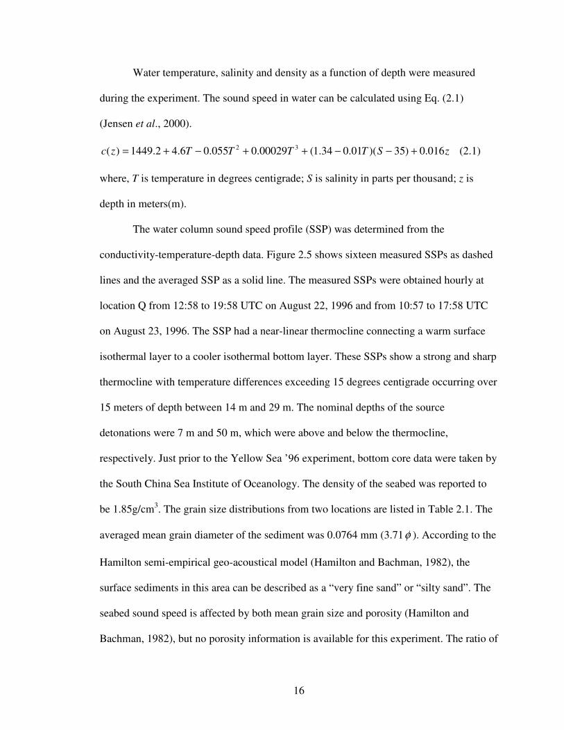
Water temperature, salinity and density as a function of depth were measured

during the experiment. The sound speed in water can be calculated using Eq. (2.1)

(Jensen et al., 2000).

zSTTTTzc 016.0)35)(01.034.1(00029.0055.06.42.1449)( 32 +−−++−+= (2.1)

where, T is temperature in degrees centigrade; S is salinity in parts per thousand; z is

depth in meters(m).

The water column sound speed profile (SSP) was determined from the

conductivity-temperature-depth data. Figure 2.5 shows sixteen measured SSPs as dashed

lines and the averaged SSP as a solid line. The measured SSPs were obtained hourly at

location Q from 12:58 to 19:58 UTC on August 22, 1996 and from 10:57 to 17:58 UTC

on August 23, 1996. The SSP had a near-linear thermocline connecting a warm surface

isothermal layer to a cooler isothermal bottom layer. These SSPs show a strong and sharp

thermocline with temperature differences exceeding 15 degrees centigrade occurring over

15 meters of depth between 14 m and 29 m. The nominal depths of the source

detonations were 7 m and 50 m, which were above and below the thermocline,

respectively. Just prior to the Yellow Sea ’96 experiment, bottom core data were taken by

the South China Sea Institute of Oceanology. The density of the seabed was reported to

be 1.85g/cm3. The grain size distributions from two locations are listed in Table 2.1. The

averaged mean grain diameter of the sediment was 0.0764 mm (3.71φ ). According to the

Hamilton semi-empirical geo-acoustical model (Hamilton and Bachman, 1982), the

surface sediments in this area can be described as a “very fine sand” or “silty sand”. The

seabed sound speed is affected by both mean grain size and porosity (Hamilton and

Bachman, 1982), but no porosity information is available for this experiment. The ratio of

17

the seabottom sound speed to the sound speed in water column near the seabed is

calculated, based solely on the mean grain size, using Jackson and Richardson’s

empirical relations (2006).

23109476.103956.0190.1 ZZ MMRatio −×+−= (2.2)

where, ZM is the mean grain size in φ . Substituting ZM =3.71φ into Eq. (2.2), the

speed ratio is 1.07. Figure 2.5 shows that the sound speed in the water column near the

seabed is around 1480 m/s. Thus, the seabottom sound speed is around 1584m/s. A

similar result is obtained by Dahl and Choi (2006).

Table 2.1. The grain size distributions from two locations at the YS ’96 site

No. Location Mean grain size Gravel Sand Silt Clay

mm φ % % % %

1 37oN, 124

o05’E 0.0769 3.70 0.9 72.5 17.7 8.9

2 37o04’N, 124

oE 0.0759 3.72 1.3 70.4 15.9 12.4

Figure 2.5 Sound speed profiles at location Q, showing a strong and sharp thermocline.

18

2.2 Shallow Water ’06 Experiment Conducted Off the New Jersey Coast: SW ’06

The Shallow Water ‘06 experiment was a comprehensive ocean acoustics and

physical oceanography experiment conducted over seven weeks in the summer of 2006.

This experiment was focused on a 40-by-50-kilometer patch of ocean about 100 miles

east of Atlantic City, N.J (See figure 2.6). This large scale experiment included six

research vessels (R.V.s), more than 50 scientists from 12 institutions, 62 moorings, 350

assorted oceanographic sensors, an airplane, space satellites, and robotic undersea gliders

(See figure 2.7). Figure 2.8 shows the six research vessels. In this thesis, the acoustic

signals transmitted by R.V. Knorr and R.V. Sharp are analyzed.

Figure 2.6 SW ’06 experiment area directly east of Atlantic City, NJ. (Newhall et al.,

2007)

19

Figure 2.7 SW ’06 experiment area cartoon. (Nevala and Lippsett, 2007)

Figure 2.8 The six research vessels used in the Shallow Water ’06 experiment

R/V Oceanus

R/V Knorr

R/V Endeavor

R/V Quest

R/V Tioga

R/V Sharp

20

2.2.1 Sub-experiment One in SW ’06

As part of the Shallow Water ’06 experiment, one 52-element L-shaped array

(SWAMI52) and one 32-element L-shaped array (SWAMI32) were deployed at site A

(39o 12’N, 72

o 57.97’W) and site B (39

o 3.6’N, 73

o 7.90’W) respectively (shown in

Fig.9). The water depth was about 75 m.

Figure 2.9. The path of the source ship (R/V Knorr) and the locations of the two L-shaped

arrays

The vertical line array (VLA) portion of SWAMI52 had 16 elements with an

element spacing of 4.37 m. The VLA portion of SWAMI32 had 12 elements with an

element spacing of 5.95 m. The VLA portion of both SWAMI52 and SWAMI32 covered

most of the water column. The horizontal line array (HLA) portions of SWAMI52 and

SWAMI32 had 36 elements and 20 elements respectively and were laid on the sea

Longitude - degrees

The path of the source ship

A

B

21

bottom. The HLA portion of SWAMI52 had a length of 230 m and the HLA portion of

SWAMI32 had a length of 256.43 m. The constructions of SWAMI32 and SWAMI52 are

shown in Figs. 2.10 and 2.11 respectively. Hydrophone location details are listed in Table

2.2.

SMAMI32 Mooring

Figure 2.10. The construction of SWAMI32

Figure 2.11. The construction of SWAMI52

SWAMI52 Mooring

22

Table 2.2a Depth information for VLA portion of SWAMI32

Table 2.2b Position information for HLA portion of SWAMI32

Hydrophone Number Spacing (m) From Hydrophone #13 (m)

13 0.00

14 20.32 20.32

15 19.34 39.66

16 18.40 58.06

17 17.51 75.57

18 16.67 92.24

19 15.86 108.10

20 15.10 123.20

21 14.37 137.57

22 13.67 151.24

23 13.01 164.25

24 12.38 176.63

25 11.79 188.42

26 11.22 199.64

27 10.67 210.31

28 10.16 220.47

29 9.67 230.14

30 9.20 239.34

31 8.76 248.10

32 8.33 256.43

Hydrophone Number Spacing (m) From top (m) Element depth (m)

1 1.00 11.00

2 5.95 6.95 16.95

3 5.95 12.91 22.91

4 5.95 18.86 28.86

5 5.95 24.82 34.82

6 5.95 30.77 40.77

7 5.95 36.72 46.72

8 5.95 42.68 52.68

9 5.95 48.63 58.63

10 5.95 54.59 64.59

11 5.95 60.54 70.54

12 5.95 66.49 76.49

23

Table 2.2c Depth information for VLA portion of SWAMI52

Hydrophone Number Spacing (m) From top (m) Element depth (m)

1 1.00 11.00

2 4.37 5.37 15.37

3 4.37 9.73 19.73

4 4.37 14.10 24.10

5 4.37 18.47 28.47

6 4.37 22.83 32.83

7 4.37 27.20 37.20

8 4.37 31.57 41.57

9 4.37 35.93 45.93

10 4.37 40.30 50.30

11 4.37 44.67 54.67

12 4.37 49.03 59.03

13 4.37 53.40 63.40

14 4.37 57.77 67.77

15 4.37 62.13 72.13

16 4.37 66.50 76.50

Table 2.2d Position information for HLA portion of SWAMI52

Hydrophone

Number

Spacing

(m) From Hydrophone

#17 (m)

Hydrophone

Number

Spacing

(m) From Hydrophone

#17 (m)

17 0.00 39 3.44 128.53

18 15.84 15.84 40 3.73 132.26

19 13.64 29.48 41 4.04 136.30

20 11.73 41.21 42 4.37 140.67

21 10.11 51.32 43 4.73 145.40

22 8.68 60.00 44 5.12 150.52

23 7.49 67.49 45 5.55 156.07

24 6.45 73.94 46 6.44 162.51

25 5.54 79.48 47 7.48 169.99

26 5.12 84.60 48 8.70 178.69

27 4.73 89.33 49 10.10 188.79

28 4.37 93.70 50 11.73 200.52

29 4.04 97.74 51 13.64 214.16

30 3.73 101.47 52 15.84 230.00

31 3.44 104.91

32 3.18 108.09

33 2.94 111.03

34 2.72 113.75

35 2.50 116.25

36 2.72 118.97

37 2.94 121.91

38 3.18 125.09

24

From August 29, 2006 to September 4, 2006, about 170 light bulb implosion

sources and 8 combustive sound sources (CSS) were deployed at different distances

between the source ship (R/V Knorr) and the two SWAMI arrays. The path of the source

ship is shown in Fig. 2.9. The source ship traveled along the straight line connecting

points A and B. The track was perpendicular to the HLA portion of SWAMI52 and

parallel to the HLA portion of SWAMI32 (see Fig. 2.12).

Figure 2.12. Sub-experiment one configuration

Water column sound speed profiles were determined from conductivity-

temperature-depth (CTD) data. Figure 2.13 shows the average sound speed profile

measured on September 4, 2006 (GMT). The wind speed was less than 3 m/s on

September 4, 2006 (GMT).

SWAMI52 SWAMI32

Knorr

12-element

VLA

16-element

VLA

20-element

HLA

36-element

HLA

A B

25

1460 1470 1480 1490 1500 1510 1520 1530 1540 1550

0

10

20

30

40

50

60

70

Sound Speed (m/s)

Wa

ter

Dep

th (

m)

Figure 2.13 Averaged sound speed profile on September 4, 2006

2.2.2 Sub-experiment Two in SW ’06

During the Shallow Water ’06 experiment, another L-shaped array (Shark), shown

in Fig. 2.14, was deployed by Woods Hole Oceanographic Institution at site O (39o

01.25’N, 73o 02.98’W). The water depth was about 80 m.

The vertical line array (VLA) portion of Shark had 16 elements and spanned the

water column between 13.5 m and 77.25 m depth. The horizontal line array (HLA)

portion of Shark had 32 elements and was laid on the sea bottom. The Shark mooring

diagram is shown in Figs. 2.15. The locations of hydrophones on the Shark array are

listed in Table 2.3.

26

Figure 2.14 Shark electronics battery sled (Newhall et al., 2007)

Figure 2.15 Shark mooring diagram (Newhall et al., 2007)

27

Table 2.3a Depth information for VLA portion of Shark

The VLA was shortened prior to deployment since the water depth was shallower

than the VLA was originally designed for. The lower hydrophones, numbers 13, 14, and

15, were wrapped together to reduce its length.

Hydrophone Number Spacing (m) Element depth (m)

0 13.50

1 3.75 17.25

2 3.75 21.00

3 3.75 24.75

4 3.75 28.50

5 3.75 32.25

6 3.75 36.00

7 3.75 39.75

8 3.75 43.50

9 3.75 47.25

10 7.50 54.75

11 7.50 62.25

12 7.50 69.75

13 0 77.25

14 0 77.75

15 0 77.75

28

Table 2.3b Locations of hydrophones on the HLA portion of Shark

Hydrophone Number Location Distance from Shark Body (m)

16 39 01.5156(N) 73 02.9804(W) 468

17 39 01.5074(N) 73 02.9807(W) 453

18 39 01.4993(N) 73 02.9809(W) 438

19 39 01.4912(N) 73 02.9812(W) 423

20 39 01.4831(N) 73 02.9815(W) 408

21 39 01.4750(N) 73 02.9817(W) 393

22 39 01.4669(N) 73 02.9820(W) 378

23 39 01.4588(N) 73 02.9823(W) 363

24 39 01.4507(N) 73 02.9825(W) 348

25 39 01.4426(N) 73 02.9828(W) 333

26 39 01.4345(N) 73 02.9831(W) 318

27 39 01.4264(N) 73 02.9833(W) 303

28 39 01.4183(N) 73 02.9836(W) 288

29 39 01.4102(N) 73 02.9839(W) 273

30 39 01.4021(N) 73 02.9841(W) 258

31 39 01.3940(N) 73 02.9844(W) 243

32 39 01.3859(N) 73 02.9847(W) 228

33 39 01.3778(N) 73 02.9849(W) 213

34 39 01.3697(N) 73 02.9852(W) 198

35 39 01.3616(N) 73 02.9855(W) 183

36 39 01.3535(N) 73 02.9857(W) 168

37 39 01.3454(N) 73 02.9860(W) 153

38 39 01.3373(N) 73 02.9863(W) 138

39 39 01.3292(N) 73 02.9865(W) 123

40 39 01.3211(N) 73 02.9868(W) 108

41 39 01.3129(N) 73 02.9871(W) 93

42 39 01.3048(N) 73 02.9873(W) 78

43 39 01.2967(N) 73 02.9876(W) 63

44 39 01.2886(N) 73 02.9879(W) 48

45 39 01.2805(N) 73 02.9881(W) 33

46 39 01.2724(N) 73 02.9884(W) 18

47 39 01.2643(N) 73 02.9886(W) 3

29

Several geo-acoustic inversion tracks were designed and are shown in Fig. 2.16.

From August 11, 2006 to August 15, 2006, the source ship (R/V Sharp) traveled along

those geo-acoustic inversion tracks. Chirp signals were transmitted at different distances

between the source ship (R/V Sharp) and the Shark array.

Figure 2.16 Geo-acoustic inversion tracks.

The location of Shark array is shown by the black triangle.

30

CHAPTER 3

SOUND PROPAGATION MODELS

3.1 Normal Mode Method

Sound propagation in the ocean is governed by the wave equation, with

parameters and boundary conditions descriptive of the ocean environment. Normal mode

theory is a widely used approach for modeling sound propagation in shallow water. One

of the earliest normal mode papers was published in 1948 by Pekeris (Perkeris, 1948)

who developed the theory for a simple two-layer model (ocean and sea bottom) with

constant sound speed in each layer. Its mathematical derivation based on separation of

variables can be found in Jensen’s book (Jensen et al., 2000).

The Helmholtz equation, which is the frequency-domain wave equation, can be

derived from the wave equation by use of the frequency-time Fourier transform pair. The

Helmholtz equation, rather than the wave equation, forms the theoretical basis in ocean

acoustic applications, because ocean acoustic experiments are characterized by hundreds

or thousands of interactions with any single boundary (Jensen et al., 2000).

3.1.1 Normal Modes for Range-Independent Environments

The inhomogeneous Helmholtz equation in cylindrical coordinates is given by:

r

rzzp

zcz

p

zzz

r

pr

rr

s

π

δδω

ρρ

2

)()(

)()

)(

1()()(

12

2 −−≈+

∂

∂

∂

∂+

∂

∂

∂

∂ (3.1)

where p is acoustic pressure, ρ is density, c is sound speed, sz is source depth (Jensen et

al., 2000).

31

The technique of separation of variables is used to solve the Helmholtz equation. The

right hand side of Eq. (3.1) is set to zero, to obtain the unforced Helmholtz equation:

0)(

))(

1()()(

12

2

≈+∂

∂

∂

∂+

∂

∂

∂

∂p

zcz

p

zzz

r

pr

rr

ω

ρρ (3.2)

Application of separation variables ( )()(),( zrRzrp Ψ= ) into Eq. (3.2), yields

0)()(

1)(

1)(

112

2

=

Ψ+

Ψ

Ψ+

zcdz

d

zdz

dz

dr

dRr

dr

d

rR

ω

ρρ (3.3)

In Eq. (3.3), the component in the first bracket is a function of r only and the component

in the second bracket is a function of z only. Equation (3.3) is satisfied only if each

component is equal to a constant. The separation constant is defined as 2

ck . Using the

component in the second bracket of Eq. (3.3), yields

0)()(

)(

)(

1)( 2

2

2

=Ψ

−+

Ψzk

zcdz

zd

zdz

dz c

ω

ρρ (3.4)

In a shallow water waveguide, the boundary condition at the pressure release surface:

0)(0

=Ψ=z

z (3.5)

The boundary condition of continuity of sound pressure and normal velocity at the

bottom interface:

−+ ==Ψ=Ψ

HzHzzz )()( (3.6)

−+ ==

Ψ=

Ψ

HzHzdz

zd

dz

zd )(1)(1

ρρ (3.7)

where H is the water depth; the notation +→ Hz denotes the limit as z tends to the

boundary from the bottom layer; the notation −→ Hz denotes the limit as z tends to the

boundary from the water.

32

The general solution of Eq. (3.4) in the seabottom (z>H) can be written as

zz

Hz

bb eBeBzγγ

21)( +=Ψ −

> (3.8)

where,

2

2

−≡

b

cbc

kω

γ (3.9)

and bc is the seabed sound speed. If bγ is assumed to be positive, then 02 =B because

of the bounded solution at infinity.

The boundary conditions (3.6) and (3.7) become

HbeBHγ−=Ψ 1)( (3.10)

b

H

bbe

Bdz

Hd

ρ

γ

ρ

γ−

−=Ψ

1)(1

(3.11)

where, bρ is the seabed density. By dividing Eqs. (3.10) and (3.11), the boundary

condition is obtained:

0)(

)(2

2

=Ψ

−

+Ψdz

Hd

ck

H

b

c

b

ωρ

ρ (3.12)

Equation (3.4) with boundary conditions (3.5) and (3.12) is a Sturm-Liouville eigenvalue

problem with eigenvalues cnk , and eigenfunction )(znΨ , where n is the mode number

(Katsnelson and Petnikov, 2002). This Sturm-Liouville eigenvalue problem is singular,

because the boundary condition Eq. (3.12) involves the eigenvalue in a square root

function and introduces a branch cut in the eigenvalue plane.

Jensen et al. (2000) obtain the solution to the Helmholtz equation:

∫∑ −ΨΨ==

EJPCcnn

M

n

sn

s

rkHzzz

izrp )()()(

)(4),( ,

)1(

0

1ρ (3.13)

33

where, )( ,

)1(

0 rkH cn is the zero order Hankel function of the first kind and ∫ EJPC is the

branch cut integral (Ewing, Jardetzky, and Press, 1957), which is introduced by the

boundary condition (3.12).

Equation (3.13) includes a mixed spectrum composed of a discrete and a

continuous part. The discrete spectrum involves a sum of modes while the continuous

spectrum involves an integral over a continuum of points in the eigenvalue plane. The

contribution of the integral can generally be neglected at comparatively long distances

(Jensen et al., 2000; Katsnelson and Petnikov, 2002). Equation (3.13) becomes

)()()()(4

),( ,

)1(

0

1

rkHzzz

izrp cnn

M

n

sn

s

ΨΨ≈ ∑=ρ

(3.14)

The Hankel function can be approximated to its asymptotic form shown in Eq. (3.15) if

1, >>rk cn

riki

cn

cncnee

rkrkH ,4

,

,

)1(

0

2)(

π

π

−

≈ (3.15)

Combining (3.14) and (3.15) together, the following solution to the Helmholtz equation is

obtained.

rk

ezze

z

izrp

cn

rik

n

M

n

sn

i

s

cn

,1

)4/(,

)()(8

1

)(),( ΨΨ≈ ∑

=

− π

πρ (3.16)

In Eq. (3.16), eigenvector )(znΨ is also named as mode depth function and it has the

orthogonality property:

mnnm dzzzz δρ =ΨΨ∫∞

)(/)()(0

(3.17)

where, the integral interval includes the water column and the sediment.

34

The eigenvalue cnk , is a complex number:

nncn ikk β+=, (3.18)

where, nk is the horizontal wave number and nβ is the modal attenuation coefficient.

The horizontal wave number can be used to define the group and phase velocity.

The group velocity of the nth

mode is:

n

n

gdk

dV

ω= (3.19)

The phase velocity of the nth

mode is:

n

n

pk

Vω

= (3.20)

The group velocity represents the energy transport velocity of a mode, and the phase

velocity represents the horizontal velocity of a particular phase in the plane wave

representation of a mode (Jensen et al., 2000).

To compute the sound field using normal mode theory, the eigenvector )(znΨ and

eigenvalue cnk , need to be found. For a known environment, )(znΨ and cnk , can be

obtained using a normal mode model, such as KRAKEN (Porter, 1992). KRAKEN,

developed by Michael Porter, is a normal mode propagation code. It uses a fast finite

difference method to accurately determine the eigenvector )(znΨ and eigenvalue cnk , . It

consists of a combination of several numerical procedures, such as bisection method and

Richardson extrapolation (Porter and Reiss, 1984). As an example, figure 3.1 shows the

first four mode shapes in YS ’96 at 200 Hz obtained using KRAKEN with the range-

independent averaged sound speed profile of figure 2.5.

35

Normally, transmission loss (TL) rather than the complex pressure field is used to

study the sound propagation. TL is defined by Eq. (3.21)

)1(

),(log20

0 =−=

rp

zrpTL (3.21)

)1(0 =rp is the sound pressure at 1 m from the source.

Substituting Eq. (3.17) into Eq. (3.21), yields

cn

rik

n

M

n

sn

s k

ezz

z

rzrTL

cn

,1

,

)()()(

/2log20),( ΨΨ−≈ ∑

=ρ

π (3.22)

The incoherent TL is defined by:

∑=

ΨΨ−≈

M

n cn

nsn

s

Inc

k

zz

z

rzrTL

1

2

,

)()(

)(

/2log20),(

ρ

π (3.23)

In some shallow water problems, where the modes are bottom-interacting, a simulated TL

obtained by using an incoherent modal summation is compared with measured

experimental data that is averaged over frequency. The detailed interference fine structure

predicted by the coherent TL calculation is not always physically meaningful (Jensen et

al., 2000).

Figure 3.2 shows the comparison between coherent and incoherent TL as a

function of range using the range-independent averaged sound speed profile in figure 2.5.

The source depth is 50 m, the receiver depth is 7 m and the frequency is 100Hz.

36

Figure 3.1 First four mode shapes at the YS ’96 site (200 Hz) using range-independent

sound speed profile.

37

Figure 3.2 Transmission Loss as a function of range at 100 Hz

38

3.1.2 Normal Modes for Range-Dependent Environments

The Normal mode method is primarily suitable for range-independent

environments. However, it can also solve range-dependent problems by dividing the

range axis into a number of segments and approximating the field as range-independent

within each segment. The boundary condition at the interface of two segments is satisfied

by the continuity of sound pressure and normal velocity. Finally, the range-independent

solution within each segment is ‘glued’ together to solve the range-dependent problem

(Jensen et al., 2000).

Figure 3.3 shows that the range-dependent problem is divided into M segments in

range. The general solution in the jth segment can be written as follows (Evans, 1983):

[ ] )()(2ˆ)(1ˆ),(1

zrHbrHazrpj

n

N

n

j

n

j

n

j

n

j

n

j Ψ×+=∑=

(3.24)

where, ))(exp()(

)()(1ˆ

1,

1

1,

)1(

0

,

)1(

0

−

−

−

−≈= j

j

cn

j

j

j

cn

j

cnj

n rrikr

r

rkH

rkHrH (3.25)

))(exp()(

)()(2ˆ

1,

1

1,

)2(

0

,

)2(

0

−

−

−

−−≈= j

j

cn

j

j

j

cn

j

cnj

n rrikr

r

rkH

rkHrH (3.26)

=

=

+

+

1

1

11

11

1

1

43

21...

43

21

43

21

n

n

nn

nn

j

n

j

n

j

n

j

n

j

n

j

n

j

n

j

n

j

n

j

n

j

n

j

n

b

a

RR

RR

RR

RR

b

a

RR

RR

b

a (3.27)

Equations (3.25) and (3.26) are the scaling of the Hankel functions. This can avoid

overflow for the modes, which involve growing and decaying exponentials. Equation

(3.27) shows a recursive relation, R is the propagator matrix.

j

n

j

n

j

n

j

n HCCR 1)ˆ~(

2

11 += ; (3.28)

39

j

n

j

n

j

n

j

n HCCR 2)ˆ~(

2

12 −= ; (3.29)

j

n

j

n

j

n

j

n HCCR 1)ˆ~(

2

13 −= ; (3.30)

j

n

j

n

j

n

j

n HCCR 2)ˆ~(

2

14 += (3.31)

where, C~

is the matrix with entries dzz

zzc

j

j

n

j

l∫+

+ ΨΨ=

)(

)()(~

1

1

lnρ

(3.32)

C is the matrix with entries dzz

zz

k

kc

j

j

n

j

l

j

cl

j

cn

∫ΨΨ

=+

+ )(

)()(ˆ

1

1

,

,

lnρ

(3.33)

The boundary condition as ∞→r : 0=M

nb for Nn L1= ; (3.34)

The source condition at 0=r : )(

)()()(

)(4 1

1

,

)2(

0

1

1

,

)1(

01

1

1

,

)1(

0

1

rkH

rkHbrkHz

z

ia

cn

cn

ncnsn

s

n +Ψ=ρ

(3.35)

Combining (3.27), (3.34), and (3.35) yields all the j

na and j

nb . Thus, Eq. (3.24) is the

two-way coupled mode solution of range-dependent problem.

Figure 3.3 Segmentation for coupled mode formulation (Jensen et al., 2000)

40

The full two-way coupled mode formulation can be simplified to the single scatter

formulation which treats each interface in range as an independent process, thus

neglecting the higher-order multiple-scattering terms (Jensen et al., 2000). This approach

is referred as the one-way coupled mode formulation. In the one-way coupled mode

approach, the incoming wave in the left segment is assumed to be given, the solution is

purely outgoing in the right segment, i.e. 01 =+jnb . Using Eq. (3.27), gives

( ) j

n

j

n

j

n

j

n aRRb 341−

−= and ( ) j

n

j

n

j

n

j

n

j

n

j

n aRRRRa )3421(11 −+ −=

and the field in any given segment can be computed.

A range-dependent example is calculated by the one-way coupled mode method.

The sound speed profiles of this range-dependent example are shown in figure 3.4.

Sediment properties and bathymetry are range independent. The water depth is 75 m and

the source depth is 50 m. The calculated TL for this range-dependent example is shown

in Figure 3.5.

Figure 3.4 Sound speed profiles used in the range-dependent example

41

Figure 3.5 Transmission Loss using One-way coupled mode (100 Hz)

3.2 Parabolic Equation Method

The parabolic equation (PE) method (Leontovich and Fock, 1946; Fock, 1965;

Tappert, 1977; Jensen et al. 1994) is used to find a marching type of solution for range-

dependent sound propagation problems. Range dependence is handled by approximating

the medium as a sequence of range-independent regions. In the PE method, it is assumed

that outgoing energy dominates back-scattered energy. An outgoing wave equation is

obtained by factoring the operator in the frequency-domain wave equation. Then, a

function of an operator is approximated using a rational function to obtain an equation

that can be solved numerically (Collins, 1997).

42

Starting from the Helmholtz equation,

0)1

(1 2

2

2

=+∂

∂

∂

∂+

∂

∂+

∂

∂pk

z

p

zr

p

rr

p

ρρ (3.36)

where, )(2

22

zck

ω= is a complex wave number.

The second term (r

p

r ∂

∂1) of the Helmholtz equation is neglected due to the far-field

approximation. Thus, sound pressure p satisfies the following far-field equation in each

range-independent region (Collins, 1993):

0)1

( 2

2

2

=+∂

∂

∂

∂+

∂

∂pk

z

p

zr

p

ρρ (3.37)

Factoring the operator in eq. (3.37), yields

0)1()1( 2/1

0

2/1

0 =

+−

∂

∂

++

∂

∂pXik

rXik

r (3.38)

2

0

22

0

1kk

zzXk −+

∂

∂

∂

∂=

ρρ (3.39)

where, 0

0c

kω

= and 0c is a representative phase speed.

The outgoing wave equation is then:

pXikr

p 2/1

0 )1( +=∂

∂ (3.40)

The solution of the outgoing wave equation is

),())1(exp(),( 2/1

0 zrpXrikzrrp +∆=∆+ (3.41)

where, r∆ is the range step.

43

The exponential function in Eq. (3.41) is approximated by an n-term rational function.

Thus, Eq (3.41) becomes

),(1

1)exp(),(

1 ,

,

0 zrpX

Xrikzrrp

n

j nj

nj∏= +

+∆=∆+

β

α (3.42)

Expanding the rational function in Eq. (3.42) by partial fractions, yields

),(1

1)exp(),(1 ,

,

0 zrpX

Xrikzrrp

n

j nj

nj

++∆=∆+ ∑

= β

γ (3.43)

The product representation (3.42) is not as useful for computation as the equivalent sum

presentation (3.43) because it does not permit parallel processing.

The Range-dependent Acoustic Model (RAM by Collins, 1997) is an efficient PE

algorithm based on Eqs. (3.42) and (3.43). It is developed to solve the range-dependent

sound propagation problems. A range-dependent example is calculated by RAM. In this

example, sediment properties are range-independent. The sound speed profiles along

track 1 of sub-experiment two in SW ’06 (see figure 3.6) and the bathymetric change

along track 1 of sub-experiment two in SW ’06 (see figure 3.7) are used in the

calculation. The source depth is 43 m. The calculated TL for this range-dependent

example is shown in Figure 3.8.

44

Figure 3.6 Sound speed profiles used in PE method

Figure 3.7 Bathymetric change used in PE method

45

Figure 3.8 Transmission Loss using PE method (160 Hz)

46

CHAPTER 4

SEABED SOUND SPEED AND ATTENUATION INVERSION FOR

THE YELLOW SEA ’96 EXPERIMENT

4.1 Introduction

In this chapter: (1) modal characteristics of broadband explosive sound signals

from YS ’96 are analyzed; (2) Transmission loss as a function of range, frequency, and

depth is obtained; (3) the results are used to obtained sound speed and attenuation in the

seabottom by inversion.

The geo-acoustic properties of the seabottom are of great importance in

determining how the seabottom influences sound propagation in the ocean. Researchers

have developed many inversion techniques to estimate broadband seabottom sound speed

and attenuation. These broadband inversion techniques involve dispersion analysis of

broadband signals (Potty et al., 2000 & 2003; Li et al., 2007), measurements of modal

attenuation coefficients (Ingenito, 1973; Zhou, 1985), measurements of modal amplitude

ratios (Potty et al., 2003; Tindle, 1982; Zhou et al., 1987), TL measurements (Peng et al.,

2004; Rozenfeld et al., 2001; Dediu et al., 2007), broadband signal waveform matching

(Li and Zhang, 2000; Knobles et al., 2006 & 2008), matched field processing (Li and

Zhang, 2004; Li et al., 2004), vertical coherence of reverberation and propagation (Zhou

et al., 2004), and Hankel transform methods (Holmes et al., 2006).

As discussed by Chapman (2001), inversion techniques are divided into two

types. Inversions of the first type estimate the geophysical properties of the seabottom as

precisely as possible and construct a true picture of the seabed layering and composition.

Such detail however may be unnecessary for some sonar applications. The second type of

47

inversion seeks a simpler “effective seabed” model that is adequate for predicting the

acoustic field. This research specifically considers the second type of inversion. In this

chapter, only long-range propagation at frequencies in the 80-1000 Hz range is examined.

Steep bottom-penetrating acoustic waves contribute little to the long-range acoustic field

in the water. A site survey did not find any apparent layer structure in the bottom at the

YS’96 site (Li et al., 1991). Thus, a half-space bottom model (with an effective sound

speed, attenuation and density) is used.

In this chapter, two inversion schemes are used to obtain the effective sound

speed in the seabottom. The first scheme is based on normal mode depth functions, which

are extracted from the cross-spectral density matrix (CSDM). The CSDM is defined by

Eq.(4.1),

HPPC = (4.1)

where, P is the pressure matrix and HP is the conjugate transpose of the matrix P.

This extraction technique is accomplished without using numerical models to obtain

solutions of a sound field and without a priori knowledge of the environment. This

extraction approach has been discussed by Wolf et al. (1993), Neilsen and Westwood

(2002), Hursky et al. (1995 & 2001), Smith (1997) and Badiey et al.

(1994). In Wolf’s

paper, the source-receiver distance was fixed and the CSDM was formed by averaging

the outer products of measured sound pressure spectra over multiple frequency bins in a

narrow band. In Neilsen’s paper, the source traversed a significant range interval and the

CSDM was obtained by averaging over time. In Hursky’s paper, the CSDM was

constructed by using ambient noise from the ocean surface. In the present study, I use a

method for extracting normal mode depth functions from broadband signals received by a

48

vertical line array at a fixed propagation distance from the explosive source. CSDM-

derived mode depth functions have been used as a basis for further data analysis. The

horizontal wave numbers and seabed sound speed are inverted by finding the best match

between the extracted normal mode depth functions and the theoretical ones. The details

of this estimation process are shown in section 4.2.

In the second scheme, the dispersion characteristics of normal modes are used to

obtain the sound speed in the seabottom. The propagation of a broadband sound signal

exhibits dispersion characteristics in shallow water. The group velocities differ for

different frequencies and modes. This dispersion behavior has been successfully utilized

for inversion of the geo-acoustic parameters (Potty et al., 2000 & 2003; Li et al., 2007).

The dispersion characteristics of normal modes can be observed using time-frequency

analysis of a broadband signal measured at sufficiently long range. The modal arrival

times corresponding to various modes and frequencies can be extracted from these time-

frequency distributions. Potty et al. (2000 & 2003) used the wavelet scalogram of the

SUS signals to analyze the time-frequency behavior. Li et al. (2007) applied an adaptive

optimal-kernel time-frequency representation technique (Jones and Baraniuk, 1995) to

derive the dispersion characteristics of the normal modes from broadband acoustic

signals excited by vacuum glass spheres. In this research, this time-frequency

representation method is used to estimate the group velocity dispersion characteristics.

The seabottom sound speed is inverted by matching the calculated group velocity

dispersion curves with the experimental data.

The inverted seabottom sound speed obtained using the above two schemes is

used as a constraint condition to estimate the sound attenuation in the seabottom by three

49

methods. The first method involves measurement of individual normal mode attenuation

coefficients. Ingenito (1973) and Zhou (1985) have obtained the modal attenuation

coefficients using individual normal mode amplitudes measured at different ranges. In

this chapter, the seabottom attenuation is estimated by matching the measured modal

attenuation coefficients of the first three modes with theoretical results. The second

method is based on measured normal mode amplitude ratios. Tindle (1982), Zhou et al.

(1987) and Potty et al. (2003) have used the measured normal mode amplitude ratios to

determine the attenuation coefficient of the seabottom. A normal mode is largest when

the receiver/source depth is close to a depth where the mode depth function has a

maximum. In this research, the signal to noise ratio for a given mode is improved by

evaluating the normal mode amplitude vs. range at a receiver depth appropriate for that

mode. The measured amplitude ratios of the second, third and fourth modes to the first

mode are compared with theoretical results to obtain the seabottom sound attenuation. In

the third method, the seabottom sound attenuation is inverted by finding the best match

between the measured and modeled broadband TLs as a function of frequency, range, and

depth along two radial lines when receivers are located both above and below the

thermocline.

The remainder of this chapter is organized as follows:

In Section 4.2, the inversion of seabed sound speed by matching measured and

modeled modal depth functions is presented. In section 4.3, the seabed sound speed is

estimated using measured modal arrival times. Then the sound attenuation in the seabed

is estimated using measured modal attenuation coefficients (Section 4.4), measured

normal mode amplitude ratios (Section 4.5), and TL data (Section 4.6).

50

4.2 Seabed Sound Speed Inverted from Data-derived Mode Depth Functions

4.2.1 Method

4.2.1.1 Construction of CSDM using measured pressure over multiple-frequency bins at a

fixed source-receiver distance

The CSDM is constructed using data from the vertical line array which spans the

whole water column. The approach to forming the CSDM in this thesis uses measured

pressure spectra over multiple-frequency bins in a narrow band at a fixed source-receiver

distance (Wolf et al., 1993; Neilsen and Westwood, 2002).

According to the normal mode theory, the far field acoustic pressure excited by a

harmonic point source is given by Eq. (3.16).

rk

ezze

z

izrp

cn

rik

n

M

n

sn

i

s

cn

,1

)4/(,

)()(8

1

)(),( ΨΨ≈ ∑

=

− π

πρ (3.16)

At a certain fixed source-receiver distance 0r , an rowz

N − by columnN f − pressure

matrix P is constructed .

=

),,(...),,(),,(

............

),,(...),,(),,(

),,(...),,(),,(

00201

02022012

01021011

rfzprfzprfzp

rfzprfzprfzp

rfzprfzprfzp

P

fzzz

f

f

NNNN

N

N

(4.2)

where, 1z , 2z , … , RNz are the receiver depths, ZN is the total number of receivers,

1f , 2f , … ,fNf are the frequencies of the multiple frequency bins in a narrow band.

The bandwidth of the narrow band can be expressed as

51

1ffBfN −= (4.3)

From Eq. (3.16), the P matrix can be expressed as a product of three matrices.

FeP f

i ΛΨ= 4π (4.4)

where

ΨΨΨ

ΨΨΨ

ΨΨΨ

=Ψ

)(...)()(

............

)(...)()(

)(...)()(

)(

1

21

22221

11211

zzz NMNN

M

M

s

zzz

zzz

zzz

zρ , (4.5)

Ψ

Ψ

Ψ

=Λ

)(...00

............

0...)(0

0...0)(

)(8

2

1

0

sM

s

s

s

f

f

z

z

z

rz

N

πρ , (4.6)

=

)(...

)()(

............

)(...

)()(

)(...

)()(

1

,

)(

2,

)(

1,

)(

,2

)(

2,2

)(

1,2

)(

,1

)(

2,1

)(

1,1

)(

0,02,01,

0,202,201,2

0,102,101,1

fM

fNcMN

M

cMN

M

cMN

f

fNccc

f

fNccc

NcN

rfik

cN

rfik

cN

rfik

Nc

rfik

c

rfik

c

rfik

Nc

rfik

c

rfik

c

rfik

f

fk

e

fk

e

fk

e

fk

e

fk

e

fk

e

fk

e

fk

e

fk

e

NF

(4.7)

Thus, the cross-spectral density matrix C is given by

HH

f

H

f

HFFPPC ΨΛΛΨ== (4.8)

52

4.2.1.2 The relationship between singular value decomposition (SVD) of the CSDM and

the normalized mode depth functions

The off-diagonal element of HFF can be expressed by

)))()((exp()()(

10

1

rfkfkifkfkN

D jmjn

N

j jmjnf

nm

f

−=∑=

, (4.9)

where, nm ≠ .

In this chapter, nmD is assumed to be negligibly small at a sufficiently long range. The

error caused by this assumption will be discussed in section 4.2.2. If nmD is

approximately zero, Eq. (4.8) becomes

HC ΨΣΨ= (4.10)

where, H

f

H

f FF ΛΛ=Σ . Σ is a matrix with nonnegative numbers on the diagonal

and zeros off the diagonal.

In Eq. (4.10), the columns of Ψ are the orthogonal, normalized mode depth

functions,

mn

D b

nm

D

nm dzz

zzdz

z

zzδ

ρρ=

ΨΨ+

ΨΨ∫∫∞

)(

)()(

)(

)()(

0

(4.11)

where D is the depth of the water column.

The second term in Eq. (4.11) is defined as

dzz

zz

D b

nmnm ∫

∞ΨΨ

=)(

)()(

ρσ (4.12)

53

The calculation in section 4.2.2 shows that nmσ is close to zero and negligible. If nmσ is

approximately zero and the receivers span the whole water column and sufficiently

sample the propagating modes in depth, then Eq. (4.12) can be rewritten as

mn

N

i i

iinimz

z

zzzδ

ρ≈

∆ΨΨ∑

=1 )(

)()( (4.13)

where zN is the number of the receivers and iz∆ is the depth difference between (i+1)th

and ith

receiver.

If the ith

row of Ψ in Eq. (4.5), and equivalently the ith

row of P in Eq. (4.2), are

multiplied by )( iz∆ , then Eq. (4.13) becomes

Ι=ΨΨH (4.14)

The CSDM, defined by Eq. (4.1), is obviously a Hermitian matrix. It can be

decomposed by SVD (Horn and Johnson, 1991).

HUUC Σ=

(4.15)

where, the columns of U are the orthonormal eigenvectors of C.

Ι=UUH

(4.16)

Comparing Eqs. (4.10) and (4.14) with Eqs. (4.15) and (4.16), researchers

recognized that the eigenvectors of the CSDM obtained by SVD correspond to the mode

shapes ( Ψ=U ).

4.2.1.3 Algorithm for estimating seabottom sound speed

Jensen et al. have divided the water column into N equal intervals to construct a

mesh of equally spaced points ihzi = , i=0,1……N, where h is the mesh width given by

54

NDh /= (see figure 4.1). Based on the finite difference mesh, a depth-separated finite

difference wave equation can derived from Eq. (3.4)

0)()(

)(

)(

1)( 2

2

2

=Ψ

−+

Ψzk

zcdz

zd

zdz

dz c

ω

ρρ (3.4)

If the density in the water column is constant, Eq. (3.4) becomes

0)()(

)( 2

2

2

2

2

=Ψ

−+

Ψzk

zcdz

zdc

ω (4.17)

Starting with the Taylor series expansion, the forward and backward difference

approximations for the first derivative are obtained.

Forward: h

zz

dz

zd jjj )()()( 1 Ψ−Ψ≈

Ψ + (4.18)

Backward: h

zz

dz

zd jjj )()()( 1−Ψ−Ψ≈

Ψ (4.19)

Adding Eq. (4.18) and Eq. (4.19) yields the centered difference approximation to the

second derivative,

2

11

2

2 )()(2)()(

h

zzz

dz

zd jjjj +− Ψ+Ψ−Ψ≈

Ψ (4.20)

Using Eqs. (4.17) and (4.20) yields the depth-separated finite difference wave equation

)()(

2)()(2

2

22

11 jn

i

jj zkzc

hzz Ψ

−−+Ψ−=Ψ −+

ω (4.21)

55

Figure 4.1 Finite-difference mesh (Jensen et al., 2000)

Given ssp in the water column and two initial values for )0(Ψ and )(hΨ , the

mode depth functions from the sea surface to the seabed can be calculated for all values

of wave number kn by Eq. (4.21). This is called the shooting method (Hursky, 2001). The

particular wave number kn, which corresponds to the data-derived mode, is obtained by

seeking a minimum of the cost function

∑=

Ψ−Ψ=N

i

nininn kzzk1

2)),()(ˆ()(F (4.22)

where )(ˆin zΨ is the n

th data-derived mode.

In the shooting method, the mode that matches the data-derived mode is produced

without knowing the seabed properties.

The boundary condition at the seabottom is satisfied by matching the impedance

of the half-space bottom model with the impedance calculated from the mode depth

functions obtained by this shooting method. The seabottom sound speed corresponding to

h

Sea surface

Sea bottom

56

the mode that best matches the data-derived mode is selected. A detailed description of

this estimation process is shown in figure 4.2.

57

Figure 4.2 Estimation process for obtaining seabed sound speed using data-derived mode

shape

Assume and SSP is given in Fig. 2.5

Depth-separated finite difference wave equation

Plug into

can be calculated for all values of k

Cost function:

Plug into

Wave number k corresponding to the inverted mode shape

)(ˆin zΨ

Minimized

0)( 0 =Ψ zn

1)( 1 =Ψ zn

)()(

2)()(2

2

22

11 jn

i

jj zkzc

hzz Ψ

−−+Ψ−=Ψ −+

ω

∑=

Ψ−Ψ=N

i

nininn kzzk1

2)),()(ˆ()(F

)(zΨ

The impedance from the mode depth functions

The impedance of the three-parameter bottom model

Matched

bottomzz

wwater

zZ

=Ψ

Ψ−=

δδ

ρ

/

Where

)/(85.1 3cmgb =ρ

from core analysis

Plug into

2

2 /

Ψ−

Ψ−

=

w

b

b

zk

C

ρ

δδρ

ω

58

4.2.2 Estimation of seabed sound speed using simulated data

In order to predict how this estimation process works with experimental data,

simulated sound fields were generated using KRAKEN. The input seabed sound speed

for KRAKEN was 1588 m/s and other input parameters, including the sound speed

profile in water column, water depth (75 m), source depth (50 m), seabed density

(1.85g/cm3), are the same as those measured in the YS ’96 experiment. Thus, the

simulations reflect realistic experimental conditions.

The simulated sound fields, containing noise (SNR=10dB), are used to form the

CSDM. Sound pressure fields from 70 Hz to 130 Hz with a frequency step of 1.5 Hz are

calculated and the sound pressure matrix P (Eq. 4.2) with 41 columns is constructed.

Using Eq. (4.1), the simulated CSDM is obtained. Mode extraction from CSDM depends

on the distance between the source and the receiver array. The effect of the distance on

the inverted mode shapes is studied. In figures 4.3-4.5, black solid lines represent the first

mode shape from KRAKEN. Red circles in figures 4.3, 4.4, and 4.5 represent the derived

first mode shapes from the SVD of CSDM obtained at distances of 16.0 km, 26.7 km, and

53.5 km respectively. These figures show that as the distance increase, the mode shape

from the SVD of CSDM improves. In figure 4.6, the difference between the mode shape

from KRAKEN and from the SVD of CSDM as a function of distance is shown. The

difference is decreased with increasing range. Based on the derived mode shapes from the

SVD of CSDM in figures 4.3-4.5, the inverted bottom sound speed is obtained by the

shooting method at three ranges (16.0 km, 26.7 km, and 53.5 km) and listed in Table 4.1.

The results in Table 4.1 show that the inverted sound speed is 1584.5 m/s with an error of

59

3.5 m/s at 53.5 km. Therefore, our simulation indicates that the process of estimating

seabed sound speed shown in Fig. 4.2 is reliable at a distance of 53.5 km.

Figure 4.3 Comparison of the first mode shape at 16.0 km

60

Figure 4.4 Comparison of the first mode shape at 26.7 km

Figure 4.5 Comparison of the first mode shape at 53.5 km

61

Figure 4.6 Difference between the mode shape from KRAKEN and from SVD of the

CSDM

Table 4.1 Seabottom sound speed inverted from simulated data

Range Inverted Bottom

Sound Speed

Input Bottom

Sound Speed

Estimation

Error

16.0km 1572.7m/s 1588m/s -15.3m/s

26.7km 1578.4m/s 1588m/s -9.6m/s

53.5km 1584.5m/s 1588m/s -3.5m/s

62

The errors shown in Table 4.1 are mainly caused by two assumptions. First, the

magnitude of nmD , defined by Eq. (4.9), is assumed to be negligibly small at sufficiently

long range. Second, nmσ , defined by Eq. (4.12), is approximately zero, and the receivers

span the whole water column so that the orthogonality condition, Eq. (4.13), is satisfied.

Based on the simulated sound field, the magnitude of nmD is calculated and listed

in Table 4.2. The calculation results show that the estimation error caused by the first

assumption is less than 3.5m/s at 53.5km.

Table 4.2 Magnitude of nmD at 16.0km, 26.7km and 53.5km

The calculated group velocities, wave numbers and modal attenuation coefficients

( nβ ) for the three modes at 100 Hz are listed in Table 4.3 (there are only three

propagating modes at 100 Hz).

Table 4.3 Group velocities, wave numbers and modal attenuation coefficients at 100Hz

Range ( 0r ) 12D 13D 23D 231312 DDD ++ Estimation

Error

16.0km 0.14 0.16 0.21 0.51 -15.3m/s

26.7km 0.08 0.09 0.14 0.31 -9.6m/s

53.5km 0.08 0.18 0.02 0.28 -3.5m/s

Mode(n) 1 2 3

nV (m/s) 1475.9 1464.6 1447.2

nk (m-1

) 0.425570 0.416092 0.405712

nβ (m-1

) 61046.6 −× 6107.19 −× 6105.38 −×

63

The normal-mode attenuation coefficient for the nth

mode can be expressed by the

integrals (Koch et al., 1983).

∫∫ Ψ+Ψ=∞ D

n

nD

nb

b

b

n

n dzzck

dzzck

0

22 )()( ραω

ραω

β (4.23)

where bα is the sound attenuation in the seabottom, and α is the sound attenuation in

water column.

The normal-mode attenuation coefficient due to seabottom attenuation can be

expressed by the first integral in Eq. (4.23). Comparing Eq. (4.12) and the first integral in

Eq. (4.23), the relations between )( mnnm =σ and modal attenuation coefficients are

obtained.

nnb

b

b

n

nck

σραω

β ×> 2

(4.24)

where ∫∞

Ψ=

D b

nnn dz

z

ρσ

)(2

(4.25)

Substituting the wave numbers and modal attenuation coefficients at 100 Hz listed in

Table 4.3 into Eq. (4.24), yields

00039.011 <σ , 0012.022 <σ , and 0022.033 <σ .

Since, },max{)( nnmmmn mn σσσ ≤≠ (4.26)

0012.012 <σ , 0022.013 <σ and 0022.023 <σ

The calculation results show nmσ is close to zero and negligible at 100 Hz.

64

4.2.3 Estimation of seabed sound speed using experimental data from YS ’96

4.2.3.1 Mode extraction from vertical line array data

Before applying the mode extraction technique to the Yellow Sea ’96 experiment,

the appropriateness of the experimental setup is examined. The 32-element vertical line

array in the Yellow Sea ’96 experiment spanned nearly the entire water column with

negligible array tilt and sufficiently dense element spacing. The water depth was 75 m

and the array spanned the depths between 4 m and 68 m with a spacing of 2 m (See figure

2.4). Thus, the data from the 32-element vertical line array can be used to construct the

CSDM. In this chapter, the bandwidth B is selected to be 60 Hz and the central frequency

is selected to be 100Hz. There are 41 frequency bins within the bandwidth B. As

discussed in section 4.2.2, the fixed source-receiver distance r0 should be appropriately

chosen for good mode extraction results. In our data processing, r0 is chosen to be 53.5

km on the QA track, and seven explosive signals with a source depth of 50 m were

measured by the 32-element vertical line array to form the CSDM. The eigenvectors of

the CSDM correspond to the mode depth function. The extracted depth function for mode

one is shown in Fig. 4.7b by circles. The error bars in Fig. 4.7b show the standard

deviations of the extracted mode shape at different receiver depths.

65

Figure 4.7 Comparison of extracted and modeled first mode shape (100Hz)

4.2.3.2 Results of the CSDM-inverted seabottom sound speed

The SSP used in the shooting method was measured at almost the same time as

the data used for the mode extraction. For example, the SSP shown in Fig. 4.7a was

measured at 19:58 UTC on August 22, 1996. That SSP was used in the shooting method

to process the broadband explosive data measured at 19:53 UTC on August 22, 1996. A

one-to-one correspondence was achieved between the extracted mode and the modeled

mode obtained by the shooting method. The cost function is calculated for seven

broadband explosive signals measured at a distance of 53.5 km. As an example, the cost

a) b)

66

function of the first signal for the first mode as a function of seabed sound speed at 100

Hz is shown in figure 4.8. The inverted seabed sound speed at 100Hz for the first signal

is 1603.4 m/s at the minimum point of the cost function F. The CSDM-inverted seabed

sound speed and the corresponding wave number for mode one at 100 Hz are listed in

Table 4.4. Thus, the averaged inverted seabed sound speed ( bC ) is sm /151593 ± , and

the corresponding wave number for mode one at 100 Hz is 0.0000390.422561 ± . The

modeled first mode shape with a seabed sound speed of 1593 m/s at 100 Hz, calculated

by the shooting method, is shown in figure 4.7b by a solid line. The modeled shape is in

good agreement with the extracted one obtained by averaging seven broadband explosive

signals.

Figure 4.8 F as a function of seabed sound speed at 100 Hz

67

Table 4.4 Inverted results from YS ’96 experimental data

4.3 Seabed Sound Speed Inverted from Measured Modal Arrival Times

4.3.1 Method

In a shallow water wave guide, for an impulsive signal of a given frequency, each

mode has a distinct group velocity. The group velocity of the nth

mode n

gV is defined by

n

n

gdk

dV

ω= (3.19)

The group velocity of the nth

mode also satisfies (Koch et al., 1983)

dzzc

z

kVzn

n

n

g

2

0 2)(

)(

)(1 Ψ∫∞

=ρω

(4.27)

The modal group velocity varies with frequency. The arrival time difference between two

frequencies for the nth

mode at range r is given by

rfKrfVfVfT tnH

n

g

n

gn )()](/1)(/1[)( =−=∆ (4.28)

At a given distance r, for the same frequency, the arrival time difference between mode n

and mode m is given by

rfKrfVfVfT tmn

n

g

m

gnm )()](/1)(/1[)( =−=∆ (4.29)

Signal number Inverted Bottom Sound Speed (m/s) Inverted Wave Number

1 1603.4 0.4225355

2 1601.2 0.4225382

3 1611.5 0.4226174

4 1601.2 0.4226138

5 1575.2 0.4225310

6 1569.8 0.4225652

7 1589.7 0.4225688

68

where Hf is the reference frequency, which is higher than f. tnK and tmnK are the group

slowness differences.

The experimental arrival time difference ( '

nT∆ and '

nmT∆ ) at a range r and the

experimental group slowness differences ( tnK' and tmnK

' ) can be extracted from time-

frequency representation of the broadband experimental signals. The widely used short-

time Fourier transform time-frequency representation is produced by taking the Fourier

transform of broadband signals over a fixed time window. However, the resolution of the

short-time Fourier transform time-frequency representation is limited by a user specified

window length. The continuous wavelet transform provides a different approach to time-

frequency analysis. However, wavelet analysis does not give good frequency resolution

at higher frequencies. In this research, an adaptive optimal-kernel time-frequency

representation (AOK TFR) based on a signal-dependent radially Gaussian kernel is used.

Since this time-frequency representation adapts its kernel to each set of signal

components, it resolves the fine detail more sharply than the short-time Fourier transform

time-frequency representation or wavelet analysis (Marple et al., 1993). Details of the

adaptive optimal-kernel time-frequency representation algorithm can be found in Jones

and Baraniuk’s paper (1995).

If the water column SSP and the seabottom density are known, the seabottom

sound speed can be inverted by matching the calculated group slowness differences ( tnK

and tmnK ) with their experimental values ( tnK' and tmnK

' ) (Zhou et al. 1985, 1987). The

inverted seabottom sound speed is obtained by seeking a minimum of the cost function

∑∑≠

−+−=)(,

2,2, )),()(()),()((),(nmnm

btmntmn

n

btntnb cfKfKcfKfKfcL (4.30)

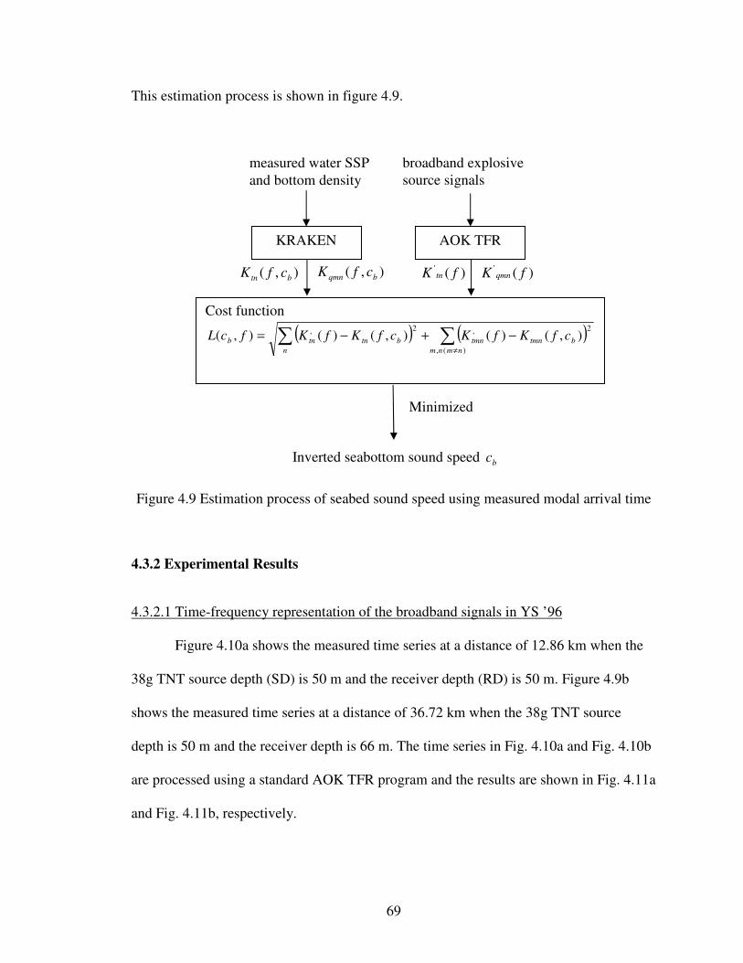
69

This estimation process is shown in figure 4.9.

Figure 4.9 Estimation process of seabed sound speed using measured modal arrival time

4.3.2 Experimental Results

4.3.2.1 Time-frequency representation of the broadband signals in YS ’96

Figure 4.10a shows the measured time series at a distance of 12.86 km when the

38g TNT source depth (SD) is 50 m and the receiver depth (RD) is 50 m. Figure 4.9b

shows the measured time series at a distance of 36.72 km when the 38g TNT source

depth is 50 m and the receiver depth is 66 m. The time series in Fig. 4.10a and Fig. 4.10b

are processed using a standard AOK TFR program and the results are shown in Fig. 4.11a

and Fig. 4.11b, respectively.

measured water SSP

and bottom density

broadband explosive

source signals

AOK TFR KRAKEN

),( btn cfK

),( bqmn cfK

)(' fK tn

)(' fK qmn

Cost function

( ) ( )∑∑≠

−+−=)(,

2,2, ),()(),()(),(nmnm

btmntmn

n

btntnb cfKfKcfKfKfcL

Minimized

Inverted seabottom sound speed bc

70

Figure 4.10 Time series of broadband explosive signals: a) at a distance of 12.86 km. b)

at a distance of 36.72 km.

71

Figure 4.11 Comparison of extracted and calculated dispersion curves: a) at a distance of

12.86 km (RD=50 m); b) at a distance of 36.72km (RD=66 m).

a)

b)

72

In figure 4.11a, at a receiver depth of 50 m, the time-frequency representation of

the shock waves (SWs) and bubble pulses (BPs) of the first mode and the third mode are

seen to have a relatively high resolution in both the time and frequency domains. The

time difference between the shock wave and the bubble pulse is approximately 0.023 s

for a 38g TNT source exploding at a depth of 50 m (Urick, 1983). The second mode can

not be identified. By way of explanation, figure 3.1 shows the four normal mode shapes

at 200 Hz for the YS ’96 experimental environment. It can be seen from figure 3.1 that

the magnitude of the second mode is near its null at a depth of 50 m, while the magnitude

of the first mode and third mode are near their maxima. Figure 4.11b shows that the

shock waves and bubble pulses of the first and the second mode are separated and easily

identified at a receiver depth of 66 m. The intensity of the second mode was enhanced,

because the magnitude of the second mode is almost at its maximum at a depth of 66 m.

4.3.2.2 Results of the TFR-inverted seabottom sound speed

The average group slowness differences tmnK' as a function of frequency,

extracted from 25 experimental signals at different distances by using time-frequency

representation, are listed in Table 4.5. In our data processing, the dispersion curve below

100Hz is not used, because the shock wave arrivals and the bubble pulse arrivals can not

be temporally resolved below 100Hz. The parameter 1'tK , defined by Eq. (4.28) between

150Hz and 600Hz, is ms /108555.0 6−× . Inputting tnK' and tmnK

' into Eq. (4.30), the

cost )( bcL as a function of seabed sound speed is obtained. For example, figure 4.12

shows the cost )( bcL as a function of seabed sound speed at 200 Hz. The inverted

seabed sound speed at 200 Hz is 1576 m/s at the minimum point of the cost function L.

73

The averaged inverted seabed sound speed is sm /151587 ± over a frequency range

from 150Hz to 400 Hz. The theoretical group velocity dispersion curves are calculated by

KRAKEN and are shown in figure 4.11 by dashed lines. The calculated curves show

good agreement with the extracted ones obtained by time-frequency representation of the

broadband explosive signals.

Table 4.5 Extracted group slowness differences (YS ‘96)

Figure 4.12 L as a function of seabed sound speed at 200 Hz

f (Hz) 200 250 300 350 400

12'tK (s/m)

6102138.2 −× 6105500.1 −× 6101844.1 −×

13'tK (s/m)

6105563.5 −× 6103436.4 −× 6104228.3 −× 6107383.2 −×

6101750.2 −×

74

The inverted seabottom sound speed from the CSDM-based inversion and the

dispersion-based inversion as a function of frequency are listed in Table 4.46 and shown

in figure 4.13. The average inverted seabottom sound speed is 1588 m/s, which is used as

a constraint condition for seabed attenuation inversion in Sec. 4.4, Sec. 4.5 and Sec. 4.6.

Table 4.6 Inverted seabed sound speed as a function of frequency (YS ‘96)

Figure 4.13 Inverted seabed sound speed as a function of frequency (YS ‘96)

f (Hz) 100 150 200 250 300 350 400

bC (m/s) 1593 1581 1576 1582 1592 1614 1576

1588 m/s

75

4.4 Seabed Attenuation Inverted from Measured Modal Attenuation Coefficients

4.4.1 Method

The normal-mode attenuation coefficient for the nth

mode can be expressed by the

integrals shown in Eq. (4.23) (Koch et al., 1983).

∫∫ Ψ+Ψ=∞ D

n

nD

nb

b

b

n

n dzzck

dzzck

0

22 )()( ραω

ραω

β (4.23)

where bα is the sound attenuation in the seabottom, and α is the sound attenuation in the

water column.

The normal-mode attenuation coefficients ( nβ ) depend on the seabed attenuation

( bα ). The seabed attenuation can thus be inverted by minimizing the difference between

the theoretical modal attenuation coefficients and the measured modal attenuation

coefficients ( '

nβ ). The experimental modal attenuation coefficients ( '

nβ ) can be extracted

from the measurements of nth

modal amplitudes at different ranges.

For a signal mode n, Eq. (3.16) expressed in decibels becomes

( ) ( )rerk

zzz

zrp n

cn

nsn

sn log20log20

)()(8

1

)(

1

log20),(log20,

βπρ

−−

ΨΨ

= (4.31)

If the source depth and receiver depth are held constant, a plot of modal amplitude

(expressed in decibels and corrected for cylindrical spreading) versus ranges should be a

straight line (Ingenito, 1973 and Zhou, 1985). Its slope is

na eK β)log20(−= (4.32)

76

If aK is obtained from the experiment, then n'β is known from Eq. (4.32). The

theoretical modal attenuation coefficients are computed using KRAKEN. A half-space

bottom model with three-parameters (sound speed, density and attenuation) is used. The

seabed sound speed is taken to be 1588 m/s, which is the average value obtained from the

CSDM-based inversion and the dispersion-based inversion. The density (1.85 g/cm3) is

taken from the core analysis. By adjusting the attenuation inputs to KRAKEN, the

normal-mode attenuation coefficient ( nβ ) is obtained. The inverted seabottom sound

attenuation is estimated by seeking a minimum of the cost function

( )∑ −=n

nbnbY2')()( βαβα (4.33)

This estimation process is shown in figure 4.14.

Figure 4.14 Estimation process of seabed sound attenuation using measured modal

attenuation coefficients

inverted seabed sound speed and

measured bottom density measured aK

KRAKEN

)( bn αβ

na eK')log20( β−=

Cost function ( )∑ −=n

nbnbY2')()( βαβα

Minimized

Inverted seabottom sound speed bα

'

nβ

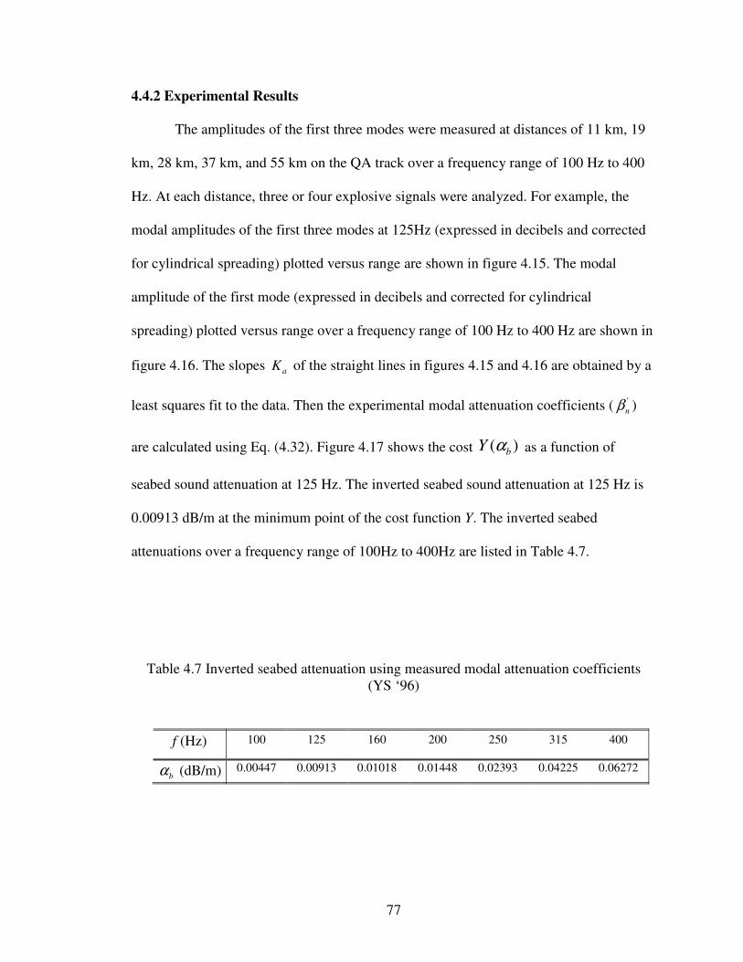
77

4.4.2 Experimental Results

The amplitudes of the first three modes were measured at distances of 11 km, 19

km, 28 km, 37 km, and 55 km on the QA track over a frequency range of 100 Hz to 400

Hz. At each distance, three or four explosive signals were analyzed. For example, the

modal amplitudes of the first three modes at 125Hz (expressed in decibels and corrected

for cylindrical spreading) plotted versus range are shown in figure 4.15. The modal

amplitude of the first mode (expressed in decibels and corrected for cylindrical

spreading) plotted versus range over a frequency range of 100 Hz to 400 Hz are shown in

figure 4.16. The slopes aK of the straight lines in figures 4.15 and 4.16 are obtained by a

least squares fit to the data. Then the experimental modal attenuation coefficients ( '

nβ )

are calculated using Eq. (4.32). Figure 4.17 shows the cost )( bY α as a function of

seabed sound attenuation at 125 Hz. The inverted seabed sound attenuation at 125 Hz is

0.00913 dB/m at the minimum point of the cost function Y. The inverted seabed

attenuations over a frequency range of 100Hz to 400Hz are listed in Table 4.7.

Table 4.7 Inverted seabed attenuation using measured modal attenuation coefficients

(YS ‘96)

f (Hz) 100 125 160 200 250 315 400

bα (dB/m) 0.00447 0.00913 0.01018 0.01448 0.02393 0.04225 0.06272

78

Figure 4.15 Attenuation of the first three normal modes at 125Hz corrected for cylindrical

spreading. The straight lines are least-squares fits.

79

Figure 4.16 Attenuation of the first normal mode corrected for cylindrical spreading

(100-400Hz). The straight lines are least-squares fits.

10dB

80

Figure 4.17 Y as a function of seabed sound attenuation at 125 Hz

81

4.5 Seabed Attenuation Inverted from Measured Modal Amplitude Ratios

4.5.1 Method

At a given distance r from the source, the ratio of the amplitude of the nth

mode to

the amplitude of the first mode can be written as

r

s

nsn

n

nne

zz

zz

k

kfR

)(

11

11

1

)()(

)()()(

ββ −

ΨΨ

ΨΨ=

(4.34)

The normal-mode attenuation coefficients ( nβ ) depend on the seabed attenuation. Thus

the theoretical modal amplitude ratio [ )(1 fRn ] in Eq. (4.34) also depends on the seabed

attenuation. The seabed attenuation can be inverted by minimizing the difference between

the theoretical modal amplitude ratios and the measured modal amplitude ratios '

1nR . By

adjusting the attenuation inputs to KRAKEN, the modal depth functions ( nΨ ), the wave

numbers (kn), and the normal-mode attenuation coefficient ( nβ ) are obtained. Then the

theoretical modal amplitude ratio is calculated by Eq. (4.34). The inverted seabottom

sound attenuation is obtained by seeking a minimum of the cost function

( )∑ −=n

nbnb RRQ2'

11 )()( αα (4.35)

This estimation process is shown in figure 4.18.

82

Figure 4.18 Estimation process of seabed sound attenuation using measured normal mode

amplitude ratios

4.5.2 Experimental results

The ratios of the amplitude of the second mode, third mode, and fourth mode to

the amplitude of the first mode ( '

21R , '

31R , and '

41R ) were extracted at distances of 13 km,

19 km, 28 km, 37 km, and 53 km on the QA track and the QG track over a frequency

range of 160 Hz to 400 Hz. At each distance, around five explosive signals were

analyzed. The nominal source depth was 50 m. Figures 4.19a and 4.19b show the

received signals filtered by a one-third-octave filter with a center frequency of 200 Hz

when the source-receiver distance is 27.48 km. The receiver depths are 40 m (Fig. 4.19a)

inverted seabed sound speed and

measured bottom density

measured '

1nR

KRAKEN

)(1 αnR

)(αnΨ , kn(a), )(αβn

r

s

nsn

n

nne

zz

zz

k

kR

)(

11

11

1

)()(

)()( ββ −

ΨΨ

ΨΨ=

Cost function ∑ −=n

nbnb RRQ'

11 )()( αα

Minimized

Inverted seabottom sound speed bα

83

and 52 m (Fig. 4.19b). In Fig. 4.19a, at a receiver depth of 40 m, the shock wave and

bubble pulse of the first mode, the second mode, and the fourth mode can be identified,

but not the third mode. This is because the magnitude of the third mode depth function is

nearly at a null at a depth of 40 m (See Fig. 3.1). At a receiver depth of 52 m, the shock

wave and bubble pulse of the first four modes can be identified, but the second mode is

very weak. This is because the magnitude of the second mode depth function is close to a

null at a depth of 52 m (See Fig. 3.1).

Figure 4.19 a) the signal received at the receiver depth of 40 m; b) the signal received at

the receiver depth of 52 m (Range=27.48km and Frequency=200Hz).

a)

b)

84

Seabed attenuation as a function of frequency from 160 Hz to 400 Hz is

determined by minimizing the difference between the theoretical modal amplitude ratios

and the measured modal amplitude ratios ( '

21R , '

31R , and '

41R ). The inverted seabed

attenuation obtained using the amplitude ratio of the second mode to the first mode ( '

21R )

was close to that obtained using the amplitude ratio of the third mode to the first mode

( '

31R ) and the amplitude ratio of the fourth mode to the first mode ( '

41R ). This implies that

the bottom attenuation is not depth dependent. Different modes penetrate into different

bottom depths. If there is apparent depth dependence in bottom attenuation, the seabed

attenuations inverted using different modes should be different. The inverted seabed

attenuations over a frequency range from 160Hz to 400 Hz are listed in Table 4.8.

Table 4.8 Inverted seabed attenuation using measured modal amplitude ratios

f (Hz) 160 200 250 315 400

bα (dB/m) 0.00841 0.02091 0.02287 0.03516 0.05761

85

4.6 Seabed Attenuation Inverted from Transmission Loss data

4.6.1 Method

Seabed attenuation can also be determined by comparing Transmission Loss data

with predictions along the propagation direction. This inversion method for attenuation

utilizes the inverted seabottom sound speed as a constraint condition. TL predictions are

calculated by KRAKEN. The inverted seabed attenuations are obtained by adjusting the

attenuation inputs to KRAKEN such that the difference between modeled and measured

TL is minimized. In this paper, TL is defined as TLbb when both the source and the

receiver are located below the thermocline (SD=50 m and RD=50 m); TLba is defined

when the source and the receiver are separately located below and above the thermocline

(SD=50 m and RD=7 m). The authors define the following cost functions:

)1(

))()()(ˆ)(ˆ(

11

2__

)( −

∑ −−−==

r

rN

ibbbaQGbbQGba

N

iTLiTLiLTiLT

bE α (4.36)

)1(

))()()(ˆ)(ˆ(

21

2__

)( −

∑ −−−==

r

rN

ibbbaQAbbQAba

N

iTLiTLiLTiLT

bE α (4.37)

)1(

))()(ˆ(

31

2_

)( −

∑ −==

r

rN

ibaQGba

N

iTLiLT

bE α (4.38)

)1(

))()(ˆ(

41

2_

)( −

∑ −==

r

rN

ibaQAba

N

iTLiLT

bE α (4.39)

where )(ˆ_ iLT QGbb -- measured TLbb at the i

th distance on the QG track,

86

)(ˆ_ iLT QGba -- measured TLba at the i

th distance on the QG track,

)(ˆ_ iLT QAbb -- measured TLbb at the i

th distance on the QA track,

)(ˆ_ iLT QAba -- measured TLba at the i

th distance on the QA track,

)(iTLbb -- calculated TLbb at the ith

distance,

)(iTLba -- calculated TLba at the ith

distance,

rN -- the number of distances.

The cost function )(1 bE α calculates the difference between the TL data and predictions

on the QG track from 3 km to 20 km, when both TLbb and TLba are taken into account.

The cost function )(2 bE α calculates the difference on the QA track from 3 km to 53.5

km, when both TLbb and TLba are taken into account. The cost function )(3 bE α calculates

the difference on the QG track from 3 km to 20 km, when only TLba is taken into account.

The cost function )(4 bE α calculates the difference on the QA track from 3 km to 20 km,

when only TLba is taken into account.

4.6.2 Experimental results

Seabed attenuation as a function of frequency from 80 Hz to 1000 Hz is

determined by comparing Transmission Loss data with predictions along the QA and QG

directions in the Yellow Sea ’96 experiment. Transmission loss data as a function of

range along two radial directions (QA and QG) were obtained by averaging the spectrum

in 1/3-octave bands. On the QG track, five shots were detonated at 18.8 km and ten shots

were detonated at each of the distances 3.9 km, 5.8 km, 9.5 km, and 12.9km. On the QA

87

track, ten shots were detonated at each of the distances 11.2 km and 19 km, and two shots

were detonated at each of the other distances. During the experiment, the sea surface was

rather smooth. In any case, sea surface effects on long-range and low-frequency sound

propagation are generally negligible. The attenuation in the water column is taken into

account using a simplified expression for frequency dependence of the attenuation in a

water column taken from Chapter 1 of Jensen et al. (1994):

24

2

2

2

23 100.3

4100

44

1

11.0103.3 f

f

f

f

fw

−− ×++

++

+×≅α [ kmdB / ] ( f in kHz) (4.40)

Based on the range independent normal mode calculation, the theoretical incoherent TL is

obtained using the averaged SSP measured at location Q (See Fig. 2.5). The results,

obtained from 80 Hz to 1000 Hz by minimizing )(1 bE α , )(2 bE α , )(3 bE α and )(4 bE α

respectively, are listed in Table 4.9. Tables 4.7, 4.8 and 4.9 show that the three

independent approaches have resulted in consistent values for seabed attenuation.

Table 4.9 Inverted seabed attenuation using TL data (YS ‘96)

f (Hz) 80 100 125 160 200 250

bα from )(1 bE α (dB/m) 0.00207 0.00447 0.00716 0.00746 0.02330 0.01999

bα from )(2 bE α (dB/m) 0.00307 0.00636 0.00756 0.01108 0.02204 0.02157

bα from )(3 bE α (dB/m) 0.00282 0.00510 0.00834 0.00867 0.02519 0.02157

bα from )(4 bE α (dB/m) 0.00257 0.00605 0.00756 0.01149 0.02015 0.01999

Averaged bα (dB/m) 0.00263 0.00549 0.00766 0.00967 0.02267 0.02078

f (Hz) 315 400 500 630 800 1000

bα from )(1 bE α (dB/m) 0.03630 0.06020 0.08407 0.13965 0.21663 0.36524

bα from )(2 bE α (dB/m) 0.03928 0.05516 0.08879 0.13370 0.22670 0.37783

bα from )(3 bE α (dB/m) 0.03928 0.05768 0.08722 0.12378 0.23678 0.37783

bα from )(4 bE α (dB/m) 0.04027 0.05516 0.08722 0.13766 0.21159 0.35894

Averaged bα (dB/m) 0.03878 0.05705 0.08682 0.13370 0.22292 0.36996

88

When the bottom attenuation was obtained by inversion from mode attenuation

coefficients, mode amplitude ratios or TLs, no particular form for the frequency

dependence was assumed, but rather an unknown (to be determined) seabottom

attenuation value (dB/m) at each frequency. For convenience, a power law form of

frequency dependence for the bottom attenuation in a given frequency band is widely

used in the ocean acoustics community:

)/(0 kHzmdBf n

b ⋅= αα (1.1)

where 0α and n are empirically derived constants. Using the “power law fitting”

method, the constants ( 0α and n ) and their uncertainties can be uniquely determined for

this data. The inverted seabottom attenuation shown in figure 4.20 can approximately be

expressed by:

)/()02.033.0( 04.086.1 kHzmdBfb ⋅±= ±α (4.41)

The standard deviations in Eq. (4.41) represent only the curve-fit uncertainties and not

any of the other uncertainties in the measurements or methods.

The sound speed and attenuation in the seabottom at the YS’96 site are very close

to the geoacoustic inversion results obtained in the Yellow Sea by Zhou (1985 and 1987),

Li et al. (2000), Li et al. (2004), Rogers et al. (2000) and Dahl and Choi (2006). The

resultant seabed sound attenuation in this paper exhibits nonlinear frequency dependence,

which is close to the results obtained by Holmes et al. (2007) and Zhou et al. (2009).

89

Figure 4.20 Sound attenuation in the bottom as a function of frequency (YS ‘96)

90

4.6.3 Comparison of TL data with predictions

TL was obtained as a function of frequency, range, and depth. Measured TL data

are compared with predictions based on the inverted seabottom acoustic parameters.

4.6.3.1 TL as a function of range and frequency

Figure 4.21 shows that the theoretical and measured TLs as a function of range are

in good agreement at 400Hz. The difference between TLbb and TLba at 10 km shows a

source-receiver depth dependence for sound propagation, which is caused by the strong

thermocline. To illustrate this phenomenon, the first four theoretical normal mode shapes

are shown in figure 3.1. The water column is divided into two regions by the strong

thermocline. The lower region is a sound duct which includes the low sound speed

portion of the water column and the thermocline itself. The other region is the isothermal

region above the thermocline. Note that the magnitudes of the lower order modes in the

upper region in figure 3.1 are much smaller than the corresponding magnitudes in the

lower region. If both the source and the receiver are located in the lower region, the lower

order modes will dominate the sound field at long range because of mode stripping. The

thermocline looks like the upper boundary of the duct and TLbb is similar to that in a

Pekeris shallow water waveguide. If the source is in the lower region and the receiver is

in the upper region, from Eq. (3.16) it is evident that only higher order modes can be

transmitted. These higher order modes have higher attenuation. Therefore, TLba is much

larger than TLbb at a long distance. The TL data for sound propagation in Fig. 4.21 clearly

exhibits such characteristics. The results for TLba for frequencies from 80 Hz to 630 Hz

are shown in figure 4.22. The theoretical and measured TLba are in reasonable agreement.

91

Figure 4.21 Comparison of TL data with predictions as a function of range along two

radial directions at 400Hz

92

Figure 4.22 Comparison of TL data with predictions as a function of range when SD=50

m and RD=7 m at 80 Hz, 160 Hz, 315 Hz, and 630 Hz

93

4.6.3.2 TL as a function of depth

Both measured TL data and calculated TL as a function of depth on the QG track

are obtained. Five shots were detonated at each point on the QG track. For example,

figure 4.23 shows the results at 100 Hz at ranges of 5.77 km and 9.55 km. Most measured

and calculated TL depth dependences are close to each other.

Figure 4.23 Comparison of TL data with predictions as a function of depth at ranges of

5.77 km and 9.55 km (SD=50 m and frequency=100 Hz)

94

4.6.4 Sensitivity analysis on the TL-based inversion of seabed sound attenuation

For example, figure 4.24 shows the cost 3E as a function of the attenuation inputs

at a frequency of 400Hz on the QG track. The inverted seabed sound attenuation is

0.0577dB/m at the minimum point of 3E . If the seabed attenuation increases or decreases

by 0.01dB/m, the increase in the cost function ( 3E ) will be around 83%. Thus, the cost

function is sensitive to the seabed sound attenuation. However, the sensitivity of the cost

function to the seabed attenuation may not reliably indicate the sensitivity of TL to the

seabed attenuation. Additional calculation results (shown in figure 4.25) are used to

discuss the sensitivity of TL to the seabed attenuation. Figure 4.25 shows the effect of

changes in seabed attenuations on TLba and TLbb. The solid lines in Fig. 4.25 show

modeled TL with a seabed attenuation of 0.0577dB/m, which corresponds to the best

match for 3E at 400Hz. The dashed lines and the dash-dot lines show modeled TL when

the seabed attenuation increases and decreases by 0.01dB/m from 0.0577dB/m,

respectively. The changes in TLbb due to this variation of seabed attenuation are not

notable from 3 km to 5 km and are less than 0.5dB from 5 km to 60 km. However, the

changes in TLba are much larger than those in TLbb. A variation of 0.01 dB/m in bottom

attenuation will cause a variation of ±2.2 dB for TLba at 20 km. The calculations show

that for the YS ’96 experiment site: (1) TLbb is insensitive to seabed sound attenuation

from 3 km to 60 km; (2) TLba or (TLba - TLbb) are sensitive to seabed sound attenuation

with increasing range; (3) The four cost functions defined in Sec. 4.6.1 may appropriately

be used for the geoacoustic inversion at the Yellow Sea ’96 experiment.

95

Figure 4.24 )(3 bE α as a function of seabed attenuation at 400Hz

96

Figure 4.25 Effect of changes in seabed sound attenuation on TL

97

4.6.5 Uncertainty of inverted seabed attenuations caused by range-dependent SSPs

in the water column

The variations of SSPs shown in figure 2.5 assumed to be caused by internal

waves. For simplicity, it is also assumed that wideband internal waves are spatially

stationary and isotropic. The SSPs measured for a long period at a given location can, in

some degree, represent the SSPs measured from many locations at a given time. Then,

the bootstrap method (Efron and Tibshirani, 1986) with 200 bootstrap samples is used to

quantify the possible effect of the SSP spatial variation in the water column on the

inverted seabed attenuation. In each bootstrap sample, sixteen water column SSPs were

selected in random order from the sixteen SSPs measured over 14 hours shown in Fig.

2.5 and assigned to sixteen locations ranging from 0 km to 52.5 km with a step of 3.5 km

along the sound propagation path. Sediment properties and bathymetry at the YS’96 site

were well assumed to be range independent. Applying coupled mode theory to each

resulting range dependent model, the seabed attenuation estimation process described in

Sec. 4.6.1 is performed for every bootstrap sample. After running 200 bootstrap samples

for each frequency, the averaged inverted seabed attenuations obtained by four functions

(1E ,

2E ,3E , and

4E ) and their standard deviations are listed in Table 4.10 and shown in

Fig. 4.20. The averaged seabed attenuations inverted from 200 bootstrap samples are

close to the results obtained in Sec. 4.6.2 over a frequency range of 80Hz to 1000Hz. For

example, the histograms of 200 bootstrap replications of inverted seabed attenuations at

100Hz and 400Hz are shown in figures 4.26 and 4.27, respectively. In each figure, the

four bootstrap histograms correspond to the inverted results obtained by four cost

functions (1E ,

2E ,3E , and

4E ), respectively. The height of each bar represents the

98

number of bootstrap samples, whose inverted seabed attenuations are within each

attenuation bin. The horizontal coordinate of the vertical solid line in each histogram

represents the inverted seabed attenuation obtained by range independent inversion with

an averaged SSP. The horizontal coordinate of the vertical dash-dot line in each

histogram represents the average inverted seabed attenuation obtained by range

dependent inversions with 200 bootstrap samples. In figures 4.26 and 4.27, the center of

each histogram (the vertical dash-dot line) is close to the vertical solid line. The

comparison of inverted seabed attenuations obtained using a range independent model

with those obtained using a range dependent model indicates that the effect of the SSP

variation in the water column on the inverted seabed attenuation is weak. Range-

independent inversion with an averaged SSP is acceptable for the Yellow Sea ’96

experiment.

Table 4.10 Inverted seabed attenuation and standard deviation

f (Hz) 80 100 125 160 200 250

Averaged bα (dB/m) 0.00250 0.00551 0.00778 0.00987 0.02267 0.02183

Standard deviation (dB/m) 0.00038 0.00091 0.00082 0.00216 0.00224 0.00225

f (Hz) 315 400 500 630 800 1000

Averaged bα (dB/m) 0.03996 0.05869 0.09543 0.14444 0.24752 0.36126

Standard deviation (dB/m) 0.00373 0.00637 0.01374 0.02448 0.05403 0.06919

99

Figure 4.26 Histograms of 200 bootstrap replications of inverted seabed attenuations by

four cost functions (1E ,

2E , 3E , and

4E ) at 100Hz

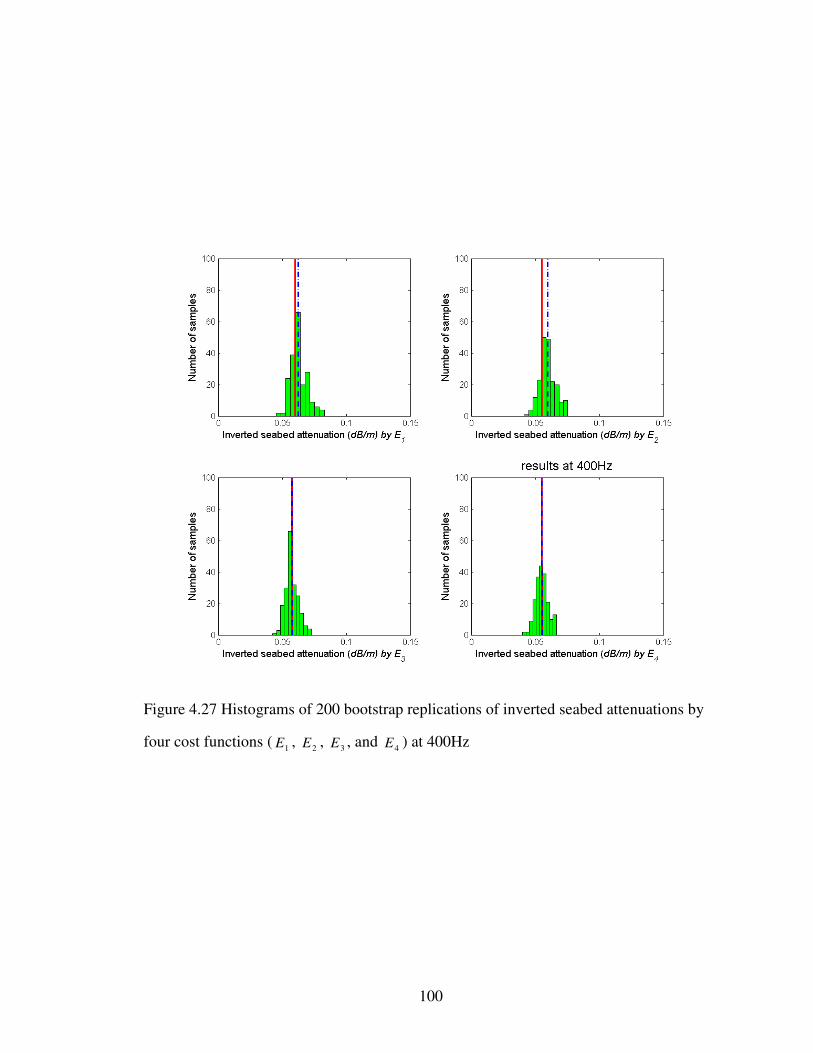
100

Figure 4.27 Histograms of 200 bootstrap replications of inverted seabed attenuations by

four cost functions (1E ,

2E , 3E , and

4E ) at 400Hz

101

CHAPTER 5

SEABED SOUND SPEED AND ATTENUATION INVERSION FOR

THE SHALLOW WATER ’06 EXPERIMENT

5.1 Introduction

In the summer of 2006, a large multidisciplinary experiment (SW ’06) was

conducted off the coast of New Jersey. Over its two month duration, a number of sub-

experiments were carried out which deal with geo-acoustic inversion. This chapter

contains analysis of combustive sound source signals, light bulb implosion signals and

chirp signals, which were transmitted from the two research vessels (Knorr and Sharp)

and measured by three L-shaped arrays (SWAMI32, SWAMI52, and Shark). The goals

of this chapter are: (1) to analyze modal characteristics of broadband explosive sound

signals; (2) to study the characteristics of three dimensional (3D) spatial coherence; (3) to

obtain TLs as a function of range, frequency, and depth; (4) to invert sound speed and

attenuation in the seabottom using the data from (1); (5) to validate the resultant geo-

acoustic parameters using spatial coherence data and TL data obtained from (2) and (3).

In Chapter 4, no apparent bottom layer structure was found by a site survey at the

YS ’96 site (Li et al., 1991), a half-space bottom model (with an effective sound speed,

attenuation and density) was hence used for the YS ’96 experimental data. The cost

function with one unknown geo-acoustic parameter (such as seabed sound speed and

seabed attenuation) was minimized by local optimization methods, which are

deterministic algorithms. In this chapter, site surveys by chirp sonar mapped an interface

known as the “R”-reflector over the SW’06 experimental area. The “R”-reflector is

around 20 m under the seabed and is indicated by a green line in Fig. 5.1 (Goff et al.,

102

2007). A bottom model with two layers in the seabed is used in the SW ’06 experiment

(see figure 5.2). In figure 5.2, H0 is the water depth (~70 m); H1 is the depth of the first

bottom layer (~20 m); C1U is the sound speed right below the interface of water and the

first bottom layer; C1D is the sound speed right above the interface of the first and

second bottom layer (a linear gradient of sound speed is assumed in the first bottom

layer); C2 is the sound speed in the second bottom layer; 1ρ and 2ρ are the densities of

the first and second bottom layers, respectively. Core analysis shows that 1ρ is

3/85.1 cmg and 2ρ is 3/1.2 cmg . The sound effective attenuation in the seabed ( bα )

is assumed to be same in those two bottom layers.

Since the densities of the first and second bottom layers are not sensitive to the

cost functions used in this chapter, 1ρ and 2ρ will not be determined by inversion.

Besides the seabed sound speed and attenuation, H0 and H1 are sensitive to the cost

function defined by modal arrival time differences. H0 and H1 can be estimated by

inversion. The inverted H0 and H1 are compared with their measured values from the site

survey, which is a sanity check.

103

Figure 5.1 Chirp seismic section measured during SW’06

Figure 5.2 A bottom model with two layers in the seabed

Layer1 3/85.11 cmg=ρ

Layer2 3/10.22 cmg=ρ

H0

H1 C1U

C1D

C2

Water

Sea surface

SE

Shark

SWAMI32

NW

75m

90m

104

Both local and global optimization methods have been successfully used in the

geo-acoustic inversions. Gerstoft (1995) applied a combination of genetic algorithms and

the Gauss-Newton approach to geo-acoustic inversion. The Levenberg-Marquardt

algorithm, which is a local search approach, has been used in the estimation of seabottom

properties by Neilsen (2000). Potty et al. (2003) used a hybrid scheme in the inversion

for sediment compressional wave velocity, where the best parameter vector obtained by a

GA search is further optimized using the Levenberg-Marquardt algorithm.

Both local and global optimization methods are used to find the minimum of the

cost function in the geo-acoustic inversions of the SW’06 experiment. In section 5.2, the

cost function is defined by multiple unknown parameters (sediment layer depth, seabed

sound speed in each sediment layer, and water depth). A hybrid optimization method,

including a genetic algorithm (GA) and a pattern search algorithm, is used to find the

global minimum of the cost function and to estimate those unknown parameters at the

SW ’06 site. In section 5.3, the sound speed right below the interface of water and the

first bottom layer is inverted using the data derived mode depth function by an exhaustive

local search. The inverted results obtained in sections 5.2 and 5.3 are used as a constraint

condition to estimate the sound attenuation in the seabed by matching the theoretical

modal amplitude ratios with experimental data in section 5.4.

Spatial coherence of the sound field in shallow water is sensitive to the seabed

parameters. Zhou et al. (2004) used reverberation vertical coherence data to invert the

seabed sound speed and attenuation. The experimental configuration of sub-experiment

one in SW ’06, shown in figure 2.12, offers an opportunity to simultaneously analyze the

three dimensional (3D) spatial coherence: vertical, transverse horizontal and longitudinal

105

horizontal. In section 5.5, the spatial coherence data as a function of frequency and range

are analyzed and used to validate the inverted results obtained in sections 5.2, 5.3 and 5.4.

A sensitivity analysis for the TL-based inversion of seabed sound attenuation is

given in section 4.6.4. The calculation shows that TL is sensitive to the seabed geo-

acoustic parameters when the source is located below the thermocline and the receiver is

located above the thermocline. In sub-experiment two of SW ’06, several geo-acoustic

tracks (shown in figure 2.16) were designed to obtain TL as a function of range. In

section 5.6, the inverted results obtained in sections 5.2, 5.3 and 5.4 are validated by

comparing the theoretical TL with measured data.

5.2 Seabed Sound Speed Inverted from Measured Modal Arrival Times

5.2.1 Multiple parameter inversion by a hybrid optimization approach

Measured modal arrival times were successfully used to invert the seabed sound

speed in the YS ’96 experiment. The details of this method can be found in section 4.3.1.

Five parameters (H0, H1, C1U, C1D and C2) are sensitive to modal arrival time

difference. Based on this dispersion characteristic of broadband signals, those five

parameters are used to parameterize the cost functions and are estimated by seeking a

minimum of the cost function.

∑≠

−=)(,

2, ))2,1,1,1,0(()2,1,1,1,0(nmnm

tmntmn CDCUCHHKKCDCUCHHL (5.1)

A standard hybrid optimization algorithm, which includes a genetic algorithm

(GA) and a pattern search algorithm from the MATLAB toolbox, is used to find the

minimum of the cost function. The optimum parameters obtained from the GA inversion

are used as a starting point for a local search using a pattern search algorithm, which

106

searches a set of points, called a mesh, around the current point. The mesh is formed by

adding the current point to a scalar multiple of a fixed set of vectors called a pattern.

If the pattern search algorithm finds a point in the mesh where the value of the

cost function is lower than the value at the current point, the new point becomes the

current point at the next step of the algorithm. The multiplier at the next step is called the

expansion factor and normally has a default value of 2. Thus, the mesh size at the next

step is doubled.

If none of the mesh points at the current step have a smaller cost function value

than the value at the current point, the algorithm does not change the current point at the

next step. The multiplier at the next step is called the contraction factor and normally has

a value of 0.5. Thus, the mesh size at the next step gets smaller.

Through a set of steps, the pattern search algorithm computes a sequence of points

that get closer and closer to the optimal point, which corresponds to the minimum of the

cost function.

The estimation process using hybrid optimization is shown in figure 5.3.

107

Figure 5.3 Estimation process of multiple parameters using measured modal arrival times

measured water SSP

and bottom densities

from core analysis combustive sound

source signals

AOK TFR KRAKEN

)2,1,1,1,0,( CDCUCHHfK tmn )(' fK tmn

Cost function

∑≠

−=)(,

2,))2,1,1,1,0(()2,1,1,1,0(

nmnm

tmntmn CDCUCHHKKCDCUCHHL

Minimized by GA optimization

Optimum parameters obtained from the GA optimization

Inverted H0, H1, C1U, C1D and C2

Pattern search algorithm

108

5.2.2 Estimation of multiple parameters using simulated data

In order to predict how this estimation process would work with experimental

data, simulated sound fields are generated by KRAKEN. The input parameters of

KRAKEN are listed in Table 5.1 and the input SSP is shown in figure 2.13. Theoretical

group slowness differences are calculated and listed in Table 5.2

Table 5.1 Input parameters for KRAKEN

Table 5.2 Theoretical group slowness differences

0H (m) 1H (m) UC1 (m/s) DC1 (m/s) 2C (m/s) 1ρ (g/cm

3) 2ρ (g/cm

3) bα (dB/ λ)

70 20 1600 1800 1865 1.85 2.10 0.000373

f (Hz) 30 50 70

12'tK (s/m)

5103237.5 × 5103915.2 −× 5101339.1 −×

13'tK (s/m) 5104893.6 −×

5108495.3 −×

14'tK (s/m) 5104825.6 −×

90 110 130 150 200

12'tK (s/m)

6103153.6 −× 6102026.4 −× 6102856.3 −× 6108342.2 −×

6101584.2 −×

13'tK (s/m)

5101113.2 −× 5102161.1 −× 6103637.7 −× 6101032.5 −×

6102802.4 −×

14'tK (s/m)

5108844.4 −× 5101279.3 −× 5109937.1 −× 5102351.1 −×

6108193.2 −×

15'tK (s/m)

5105401.5 −× 5104801.5 −× 5109472.3 −× 5108401.2 −×

5102118.1 −×

16'tK (s/m)

6102894.1 −× 5100047.4 −× 5107149.5 −× 5104811.4 −×

5103034.2 −×

17'tK (s/m) 5102331.2 −× 5106887.5 −×

5104448.3 −×

109

It is assumed that five parameters (H0, H1, C1U, C1D and C2) need to be

estimated from the simulated group slowness differences shown in Table 5.2. Inputting

tmnK' into Eq. (5.1), the cost L is minimized by a hybrid optimization approach, including

a genetic algorithm (GA) and a pattern search algorithm. In the GA optimization, the

search bounds for five parameters (H0, H1, C1U, C1D and C2) are listed in Table 5.3.

The search bounds are determined by a priori knowledge of those parameters. An initial

population of 40 samples is randomly generated within the search bounds for the

unknown parameters. These 40 samples are the first generation of the GA. The value of

the cost function for each sample is calculated. The smallness of the cost function value

measures the fitness of the sample. The GA creates three types of children for the next

generation. 1) Elite children: the samples in the current generation with the best fitness

values. These samples automatically survive to the next generation. 2) Crossover

children: the samples in the next generation are created by combining the vectors of a

pair of parents, which are the samples in the current generation. 3) Mutation children: the

samples in the next generation are created by introducing random changes, or mutations,

to a single parent. Here, the numbers of elite children, crossover children, and mutation

children for each generation are set at 2, 24, and 14, respectively. The best fitness

function value at each generation is the minimum of the cost function values for 40

samples at that generation. Figure 5.4 shows the minimum and average of the cost

function values for 40 samples at each generation. Through a set of generations, the

initial population evolves in order to become more fit. If there is no improvement in the

minimum of the cost function values for 10 consecutive generations, the genetic

algorithm will stop. In figure 5.4, the genetic algorithm stops at the 40th generation. The

110

cost function values for 40 samples at the 40th generation are close to the best fitness

function value. The optimum point in the parameter space corresponds to the optimum

parameters with the best fitness function value. The optimum point at the 40th generation

is used as a starting point for a local search using the pattern search algorithm. The

inverted results of multiple parameters (H0, H1, C1U, C1D and C2) are listed in Table

5.3. The results in Table 5.3 indicate that the estimation process shown in Figure 5.3 is

reliable.

Table 5.3 Search bounds and inverted results from simulated data

Figure 5.4 Minimum and average of cost function values vs. generation

H0 (m) H1 (m) C1U (m/s) C1D (m/s) C2 (m/s)

Search Bounds [68,72] [5,30] [1580,1650] [1700,1900] [1800,1900]

Inversion Results 69.94 20.02 1608.00 1803.90 1865.01

Input Value 70 20 1600 1800 1865

Difference -0.06 0.02 8.00 3.90 0.01

111

5.2.3 Estimation of multiple parameters using experimental data

5.2.3.1 Time-frequency representation of the broadband signals in sub-experiment one of

SW ’06

Figure 5.5a shows the measured time series at a distance of 16.33 km when the

combustive sound source (SD=50 m) was detonated on the BA track (shown in figure

2.9) and the receiver was the 17th

hydrophone of SWAMI52. Figure 5.5b shows the

measured time series at a distance of 16.33 km when the combustive sound source depth

(SD) was 50 m and the receiver was the 20th

hydrophone of SWAMI52, which was laid

on the seabed. The time series in Fig. 5.5a and Fig. 5.5b were processed using AOK TFR

and the results are shown in Fig. 5.6a and Fig. 5.6b, respectively. It is seen from figures

5.6a and Fig. 5.6b that the dispersion curves can not be easily identified because of the

low signal to noise ratio.

The HLA portion of SWAMI52 (hydrophone number: 17-52) was laid on the

seabed and exactly perpendicular to the direction of sound propagation. The time series

received by the hydrophones of the HLA portion of SWAMI52 are combined so that the

signal to noise ratio is enhanced and the dispersion curves can be easily identified. Figure

5.7 shows the combined time series of 36 channels on the HLA portion of SWAMI52.

The time series in Fig. 5.7 were processed using AOK TFR and the results are shown in

Fig. 5.8.

112

Figure 5.5 Measured time series of combustive sound source signals: a) the receiver is

#17 hydrophone of SWAMI52. b) the receiver is #20 hydrophone of SWAMI52.

113

Figure 5.6 TFR of measured time series of combustive sound source signals: a) the

receiver is #17 hydrophone of SWAMI52. b) the receiver is #20 hydrophone of

SWAMI52.

114

Figure 5.7 Combined time series of 36 channels on the HLA portion of SWAMI52

Figure 5.8 TFR of the time series shown in figure 5.7

115

5.2.3.2 Inverted results

The average group slowness differences tmnK' as a function of frequency,

extracted from the combined time series of 36 channels on the HLA portion of

SWAMI52 at different distances by using time-frequency representation, are listed in

Table 5.4. Inputting tmnK' into Eq. (5.1), the cost L is minimized by the hybrid

optimization approach shown in section 5.2.2. The search bounds and inverted results of

multiple parameters (H0, H1, C1U, C1D and C2) are listed in Table 5.5. The theoretical

group velocity dispersion curves are calculated using the inverted parameters and are

shown in figure 5.9 by dashed lines. The calculated curves show good agreement with the

extracted ones obtained by time-frequency representation of the broadband explosive

signals.

Table 5.4 Extracted group slowness differences (SW ‘06)

Table 5.5 Search bounds and inverted results (SW ‘06)

f (Hz) 50 60 90

12'tK (s/m)

5103896.2 −× 5105956.1 −× 5106151.0 −×

f (Hz) 65 75 90

23'tK (s/m)

5108981.2 −× 5103277.2 −× 5104519.1 −×

f (Hz) 90 100 105 115 135

34'tK (s/m)

5109414.2 −× 5102962.2 −× 5101652.2 −×

5107983.1 −× 5101516.1 −×

f (Hz) 135 140 150 160

45'tK (s/m)

5109296.1 −× 5109024.1 −× 5107240.1 −×

5105375.1 −×

H0 (m) H1 (m) C1U (m/s) C1D (m/s) C2 (m/s)

Search Bounds [65,80] [1,50] [1540,1700] [1540,1800] [1700,2100]

Inversion Results 70.8 21.8 1607.8 1795.4 1865.1

116

Time(s)

Fre

quency(H

z)

0.2 0.3 0.4 0.5 0.6 0.7 0.8 0.9 10

50

100

150

200

250

300

350

400

20

40

60

80

100

120

140

160

Figure 5.9 Comparison of extracted and calculated dispersion curves (Range=16.33 km,

SD=50 m, RD= 70.8 m)

117

5.3 Seabed Sound Speed Inverted from Data-derived Mode Depth Functions

In section 4.2.1, data-derived mode depth functions obtained from CSDM were

successfully used to invert the seabed sound speed in the YS ’96 experiment. In this

section, this inversion technique is used for sub-experiment one of the SW ’06

experiment to estimate the sound speed right below the interface of water and the first

bottom layer (C1U).

5.3.1 Mode extraction from VLA portion of SWAMI52

In SW ’06, the VLA portion of SWAMI52 spanned nearly the entire water

column and had dense element spacing. The water depth as obtained from section 5.2.3

was 70.8 m and the array spanned the depths between 11 m and 67.77 m with a spacing

of 4.37 m (See Table 2.2c). The data from the VLA portion of SWAMI52 can be used to

construct the CSDM. In this section, the bandwidth B is selected to be 8 Hz and the

central frequency is selected to be 50Hz. There are 8 frequency bins within the bandwidth

B. In our data processing, the fixed source-receiver distance r0 is chosen to be 18.96 km

along the BA track (See figure 2.9). Combustive sound source signals with a source depth

of 25 m were measured on the VLA portion of SWAMI52 to form the CSDM. Recall

from Chapter 4 that the eigenvectors of the CSDM correspond to the mode depth

function. The extracted depth function for mode one is shown by circles in Fig. 5.10b.

5.3.2 Results of the CSDM-inverted sound speed (C1U)

The SSP used in the shooting method is shown in Fig. 5.10a. The cost function is

calculated for the combustive sound source signal measured at a distance of 18.96 km on

the BA track. The cost function for the first mode as a function of C1U at 50 Hz is shown

118

in figure 5.11. The inverted C1U at 50Hz is 1606.9 m/s at the minimum point of the cost

function F, and the corresponding wave number for mode one at 50 Hz is 0.207346. The

modeled first mode shape with a C1U of 1606.9 m/s at 50 Hz, calculated by the shooting

method, is shown in figure 5.10b by a solid line. The modeled shape is in good agreement

with the extracted one. The inverted C1U (1606.9m/s) in the CSDM-based method is

close to the inverted C1U (1607.8m/s) in the dispersion-based method. The ratio of C1U

to the sound speed in water column near the seabed is 1.079.

Figure 5.10 Comparison of extracted and modeled first mode shape (50Hz)

119

Figure 5.11 F as a function of C1U at 50 Hz

120

5.4 Seabed Attenuation Inverted from Measured Modal Amplitude Ratios

In SW ’06, the CSS signals with same source depth were detonated at only three

or four ranges. Thus, measured modal attenuation coefficients and TL data will not be

used to estimate the seabed attenuation for SW ’06.

In section 4.5.1, measured modal amplitude ratios were successfully used to invert

the seabed sound attenuation for the YS ’96 experiment. In this section, the method is

applied to sub-experiment one of SW ’06. The inverted results obtained in sections 5.2

and 5.3 are used as a constraint condition to estimate the sound attenuation in the seabed

by matching the theoretical modal amplitude ratios with experimental data.

The ratios of the amplitudes of the second mode and third mode to the amplitude

of the first mode ( '

21R and '

31R ) were extracted at distances of 10.79 km, 16.33 km and

25.69km on the BA track over a frequency range of 63Hz to 400Hz. For example, Fig.

5.12 shows the received signal at 315 Hz when the source-receiver distance is 16.33 km.

The source depth was 50 m and the receiver depth was 50.3 m. The first four modes can

be identified in figure 5.12.

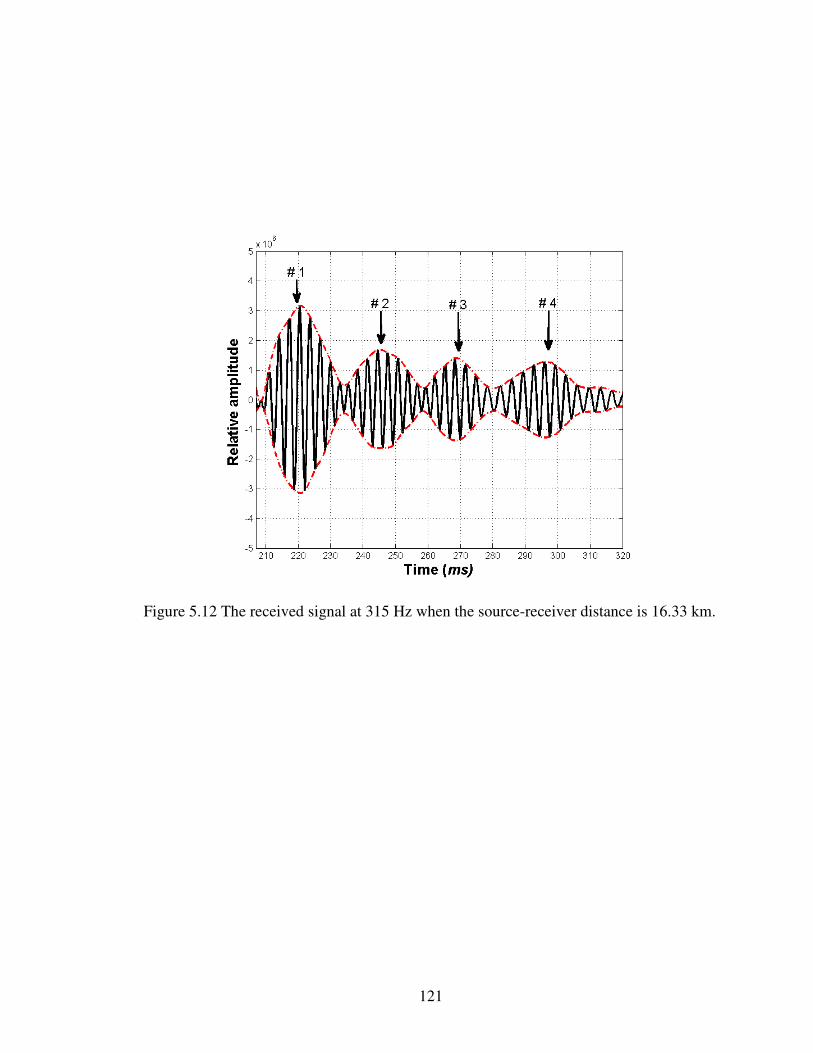
121

Figure 5.12 The received signal at 315 Hz when the source-receiver distance is 16.33 km.

122

Seabed attenuation is determined by minimizing the difference between the

theoretical modal amplitude ratios and the measured modal amplitude ratios

( '

21R and '

31R ). The inverted seabed attenuations over a frequency range of 63Hz to 400Hz

are listed in Table 5.6 and shown in figure 5.13. The inverted seabottom attenuation

shown in figure 5.13 can approximately be expressed by:

)/()08.041.0( 10.082.1 kHzmdBfb ⋅±= ±α (5.2)

Table 5.6 Inverted seabed attenuation using measured modal amplitude ratios (SW ’06)

Figure 5.13 Sound attenuation in the bottom as a function of frequency (SW ’06)

f (Hz) 63 80 100 125 160 200 250 315 400

bα (dB/m) 0.0028 0.0045 0.0059 0.0092 0.0090 0.0293 0.0355 0.0454 0.0812

123

5.5 Comparison of Spatial Coherence Data with Predictions based on Inverted

Seabottom Parameters

The spatial coherence of the sound field in shallow water is sensitive to the seabed

parameters (Zhou et al. 2004). Measured spatial coherence can thus be used to validate

the inverted seabottom parameters. The experimental configuration of sub-experiment

one in SW ’06 is shown in figure 2.12. Two L-shaped arrays (SWAMI32 and SWAMI52)

were deployed. The constructions of SWAMI32 and SWAMI52 are shown in figures

2.10 and 2.11 and Table 2.2. The source ship traveled along the straight line connecting

points A and B in figure 2.9. The HLA component of SWAMI52 was perpendicular to

the direction of sound propagation. The HLA component of SWAMI32 was parallel to

the direction of sound propagation. This configuration offered an opportunity to

simultaneously analyze the three dimensional (3D) spatial coherence: vertical, transverse

horizontal and longitudinal horizontal. The spatial coherence data as a function of

frequency and range are analyzed and used to validate the inverted results obtained in

sections 5.2, 5.3 and 5.4.

5.5.1 Spatial coherence measurements from SWAMI32 and SWAMI52 in the sub-

experiment one of SW ’06

5.5.1.1 Experimental data processing

Figure 5.14a shows the combustive sound source (CSS) signal received by the 52

hydrophones of SWAMI52 at a distance of 16.33 km. (hydrophone #18 of SWAMI52 did

not work during the experiment). Figure 5.14b shows the same combustive sound source

signal received by the 32 hydrophones of SWAMI32 at a distance of 4.79 km. The

source depth was 50 m.

124

Figure 5.14 Combustive sound source signal received by a) SWAMI52 at a distance of

16.33 km; b) SWAMI32 at a distance of 4.79 km (SD=50 m).

VLA

HLA

VLA

HLA

125

Experimental spatial coherence in this chapter is defined as the normalized cross

correlation between the sound pressures received at two spatially separated points. The

mathematical expression for the experimental spatial coherence is shown in Eq. (5.3)

∫ ∫

∫∆+ ∆+

∆+

×

−

=∆Tt

t

Tt

t

Tt

t

dttpdttp

dttptp

T

)()(

)()(

),(

2

2

2

1

21 τ

τρ (5.3)

where, τ is the time delay and T∆ is the integration time. It can be seen from figure 5.14

that the time delay is zero for the vertical coherence. Since the HLA component of

SWAMI52 was perpendicular to the direction of sound propagation, the time delay is

zero for the transverse horizontal coherence. The HLA component of SWAMI32 was

parallel to the direction of sound propagation, so the time delay for the longitudinal

horizontal coherence is given by cL /=τ , where L is the hydrophone separation and c is

the sound speed. The spatial coherence is evaluated using an integration time 426.7 ms

for SWAMI52 and 655.3 ms for SWAMI32 and is averaged over different pairs of

hydrophones with the same separation in the water. In section 5.5.1.1, all presented data

are evaluated for the stated center frequencies with a bandwidth of 100 Hz. In this

section, the coherence length is defined as the separation between two receivers,

expressed in units of the wavelength at the center frequency at which the spatial

coherence falls below 0.5. The coherence length is a measure of the angular uncertainty

caused by the transmitting medium.

An example is used here to explain the data processing. Figures 5.15a and 5.15b

show the CSS time series received by the VLA portion of SWAMI32 at depths of 46.72

m and 52.68 m respectively, when the source depth was 35 m and the source-receiver

126

range was 10.8 km. Those CSS time series have high signal to noise ratio. The signals in

Fig. 5.15a and Fig. 5.15b were filtered by a band pass filter with a center frequency of

300 Hz and a bandwidth of 100 Hz (See Fig. 5.16a and Fig. 5.16b). The normalized cross

correlation function is evaluated by Eq. (5.3). Figure 5.17 shows the normalized cross

correlation function. The spatial correlation coefficient for the two signals shown in Fig.

5.16 is seen to be 0.64.

0 0.1 0.2 0.3 0.4 0.5 0.6-5

0

5x 10

7

Am

plit

ud

e

Time (Second)

a)

0 0.1 0.2 0.3 0.4 0.5 0.6-5

0

5x 10

7

Am

plit

ud

e

Time (Second)

b)

Figure 5.15. Measured CSS time series received by the VLA portion of SWAMI32.

a) RD=46.72 m; b) RD=52.68 m.

127

0 0.1 0.2 0.3 0.4 0.5 0.6-1.5

-1

-0.5

0

0.5

1

1.5x 10

7

Am

plit

ud

e

Time (Second)

a) signal

envelope

0 0.1 0.2 0.3 0.4 0.5 0.6-1.5

-1

-0.5

0

0.5

1

1.5x 10

7

Am

plit

ud

e

Time (Second)

b) signal

envelope

Figure 5.16 The measured CSS time series of Fig. 5.15 filtered by the band pass filter

with a center frequency of 300 Hz and a bandwidth of 100 Hz.

128

-0.2 -0.15 -0.1 -0.05 0 0.05 0.1 0.15 0.2-1

-0.8

-0.6

-0.4

-0.2

0

0.2

0.4

0.6

0.8

1

No

rmaliz

ed

cro

ss

corr

ela

tion

Time (Second)

envelope

0.64

Figure 5.17 Normalized cross correlation function for two signals shown in Fig. 5.16.

129

5.5.1.2 Characteristics of observed spatial coherence

5.5.1.2.1 Range dependence of vertical coherence

Figure 5.18 shows the experimental results for vertical correlation coefficient as a

function of hydrophone separation (in units of wavelength λ) at three different ranges

(3.5 km, 7.7 km, and 10.8 km). The source was located at a depth of 35m, which was

below the thermocline. The vertical correlation coefficient was averaged over data from

six receivers which were below the thermocline. The center frequency was 100 Hz. The

data show that the coherence lengths were 0.58 λ at 3.5 km, 0.81 λ at 7.7 km and 0.96 λ

at 10.8 km. Figure 5.19 shows the measured vertical correlation coefficient as a function

of range at three different frequencies (100 Hz, 200 Hz and 300 Hz). The hydrophone

separation was 5.95 m. In Fig. 5.19, the measured vertical correlation coefficient at 200

Hz increased from -0.04 at a range of 0.8 km to 0.82 at a range of 10.8 km. Based on Fig.

5.18 and Fig. 5.19, the conclusion was drawn that the vertical coherence length in units of

wavelength increases with range. This conclusion was also obtained by Galkin et al.

(2004) and Jie Yang et al. (2007).

130

0 0.2 0.4 0.6 0.8 1 1.2 1.4 1.6 1.8 2

-0.2

0

0.2

0.4

0.6

0.8

1

Co

rre

lation

Coe

ff.

Hydrophone separation/ λ

3.5km

7.7km

10.8km

Figure 5.18 Vertical coherence at different ranges (SD=35 m and frequency = 100 Hz).

The error bars show the standard errors.

131

0 2 4 6 8 10 12-0.4

-0.2

0

0.2

0.4

0.6

0.8

1

Co

rre

lation

Coe

ff.

Range (km)

100Hz

200Hz

300Hz

Figure 5.19 Vertical coherence as a function of range at different frequencies.

(Hydrophone separation is 5.95 m).

132

5.5.1.2.2 Frequency dependence of vertical coherence

Figure 5.20 shows the experimental results for vertical correlation coefficient as a

function of hydrophone separation (in units of λ) at two different frequencies (100 Hz and

300 Hz). The source was located at a depth of 35m, which was below the thermocline.

The vertical correlation coefficient was averaged over data from nine receivers which

were located below the thermocline. The source-receiver range was 13.5 km. In Fig. 5.20,

the coherence lengths were 0.87 λ at 100 Hz, 1.39λ at 200 Hz and 1.51 λ at 300 Hz from

which it was concluded that the vertical coherence length in units of wavelength

increases with frequency.

Figure 5.20 Vertical coherence at two different frequencies

(Range=13.5 km and SD=35 m).

133

5.5.1.2.3 Range dependence of longitudinal horizontal coherence

Figure 5.21 shows the measured longitudinal horizontal correlation coefficient as

a function of hydrophone separation (in units of λ) at three different ranges (1.7 km,

4.8km, and 10.8 km). The center frequency was 300 Hz. In Fig. 5.21, the coherence

lengths were 9.0 λ at a range of 1.7 km, 11.6 λ at a range of 4.8 km, and 17.4 λ at a range

of 10.8 km. The longitudinal horizontal coherence length in units of wavelength increases

with range.

0 2 4 6 8 10 12 14 16 18 200

0.1

0.2

0.3

0.4

0.5

0.6

0.7

0.8

0.9

1

Co

rre

lation

Coe

ff.

Hydrophone separation/ λ

1.7km

4.8km

10.8km

Figure 5.21 Longitudinal horizontal coherence at different ranges

134

5.5.1.2.4 Frequency dependence of longitudinal horizontal coherence

Figure 5.22 shows the results for longitudinal horizontal correlation coefficient as

a function of hydrophone separation (in units of λ) at two different frequencies (100 Hz

and 300 Hz). The source depth was 35 m. The source-receiver range was 7.7 km. In

Figure 5.22, the coherence lengths were 7.18 λ at 100 Hz, 8.9 λ at 200 Hz and 12 λ at 300

Hz. The longitudinal horizontal coherence length in units of wavelength increases with

frequency.

Figure 5.22 Longitudinal horizontal coherence at different frequencies

135

5.5.1.2.5 Range dependence of transverse horizontal coherence

Figure 5.23 shows the measured transverse horizontal correlation coefficient as a

function of hydrophone separation (in units of λ) at four different ranges (5.8 km, 6.4 km,

8.8 km and 9.3 km). The center frequency was 200 Hz. The source depth was 25 m. In

Fig. 5.23, the transverse horizontal coherence lengths were much larger than 35 λ. There

was no apparent range dependence for the transverse horizontal coherence lengths.

0 5 10 15 20 25 30 350

0.1

0.2

0.3

0.4

0.5

0.6

0.7

0.8

0.9

1

Co

rre

lation

Coe

ff.

Hydrophone separation/ λ

5.8km

6.4km

8.8km

9.3km

Figure 5.23 Transverse horizontal coherence at different ranges

136

5.5.1.2.6 Frequency dependence of transverse horizontal coherence

Figure 5.24 shows the results for transverse horizontal correlation coefficient as a

function of hydrophone separation (in units of λ) at three different frequencies (100 Hz,

200 Hz and 300 Hz). The source was within the thermocline (SD=25 m). The source-

receiver range was 8.8 km. Figure 5.24 shows the transverse horizontal coherence lengths

were much larger than 40λ. These results agree with Carey’s theoretical calculation

(2006), in that they show a similar trend that the transverse horizontal coherence length in

units of wavelength decreases with frequency.

0 5 10 15 20 25 30 35 400

0.1

0.2

0.3

0.4

0.5

0.6

0.7

0.8

0.9

1

Hydrophone separation/ λ

Co

rre

lation

Coe

ff.

100Hz

200Hz

300Hz

Figure 5.24 Transverse horizontal coherence at different frequencies

137

5.5.1.3 Physical explanation of observed coherence results

5.5.1.3.1 Vertical and longitudinal horizontal coherence

When both source and receiver are located below the thermocline, the spatial

coherence at long-range for higher frequency should be similar to that in a Pekeris

shallow water waveguide. According to Smith (1976), the vertical and longitudinal

horizontal coherence length respectively can be expressed by

effvertical θλρ /265.0= (5.4)

effallongitudin

2/23.1 θλρ = (5.5)

where, effθ is the effective grazing angle of the sound propagation. It can be expressed by

QR

Heff =θ (5.6)

where, H is the water depth, R is the range, Q is the bottom reflection loss factor in

neper/rad. Q can be can written in the form (Weston, 1971; Buckingham, 1979)

βρ

ρ

×

−

=2

32

2

1

2

bottom

water

water

bottom

bottom

water

c

c

c

c

Q (5.7)

where, β is a measure of the seabottom attenuation in neper/rad.

β can be expressed by bottomα in dB/m.kHz

( )

= β

πα

b

bottomc

fe

2log20 (5.8)

Combining Eqs. (5.7) and (5.8), yields

138

f

c

c

c

c

Q bottom

bottom

water

water

bottom

bottom

water

αρ

ρ

×

−

=2

32

2

1

0366.0 (5.9)

In Eqs. (5.7), (5.8) and (5.9), waterc and bottomc are the sound speeds in the water and

bottom in units of km/s. waterρ and bottomρ are the densities, bottomα is the sound

attenuation in the bottom (dB/m.kHz) and f is the frequency in kHz.

Due to mode stripping (higher modes with larger grazing angles suffer greater

loss), the effective grazing angle of sound propagation decreases with increasing range.

Using Eqs. (5.4) and (5.5), the vertical and longitudinal horizontal coherence lengths in

units of wavelength increase with range at the same frequency.

In general, the bottom loss increases with frequency. For a given distance, the

higher the frequency, the smaller the effective grazing angle. Using Eqs. (5.4) and (5.5),

the vertical and longitudinal horizontal coherence lengths in units of wavelength increase

with increasing frequency at the same distance.

The frequency dependence of the vertical and longitudinal horizontal coherence

lengths, obtained when both source and receiver are located below the thermocline at

long-range for higher frequency, can also be explained by a non-linear frequency

dependence of seabed sound attenuation. If the attenuation has a non-linear frequency

dependence and varies as f n ( 1≠n ), Q of Eq. (5.9) is frequency dependent and the

vertical and longitudinal horizontal coherence lengths (in units of λ) are frequency

dependent.

139

In section 5.5.2, the frequency dependence of vertical coherence lengths is

verified by the theoretical calculation results of vertical coherence in SW ’06. The

theoretical results are calculated using the inverted results obtained in section 5.2, 5.3 and

5.4.

5.5.1.3.2 Transverse horizontal coherence

The transverse horizontal coherence is a measure of angle uncertainty of sound

propagation in the horizontal plane, or a measure of signal phase fluctuations. In shallow

water, degradation of the transverse horizontal coherence is mainly caused by water

column inhomogeneity scattering and random boundary scattering. In contrast to the

vertical and longitudinal horizontal coherence, the observed transverse horizontal

coherence decreased with increasing frequency (See Fig. 5.24). This may be explained by

the likelihood that water column inhomogeneity and random boundary scattering

increased with increasing frequency in a 100-300 Hz range at the measurement site. (Wan

et al., 2009)

5.5.2 Theoretical calculation of vertical coherence in the sub-experiment one of SW

’06

5.5.2.1 Mathematical expression

The mathematical expression for the theoretical vertical coherence is shown in

Eq. (5.10)

22

*

),(),(

),(),(),,(

rzzprzp

rzzprzprzz

∆+

∆+=∆ρ (5.10)

140

where, z is the receiver depth and z∆ is the vertical separation of a pair of hydrophones.

Using the expression for sound pressure,

rk

ezze

z

izrp

cn

rrik

n

M

n

sn

i

s

nn

,1

)4/( )()(8

1

)(),(

βπ

πρ

−

=

− ΨΨ≈ ∑ (3.16)

The numerator in Eq. (5.10) becomes

∆+ΨΨΨΨ

+∆+ΨΨΨ

=∆+

∑

∑

≠

+−−

=

−

mn cmcn

rrkki

msmnsn

mn cn

r

nnsn

s

kk

ezzzzz

k

ezzzz

zrrzzprzp

mnmn

n

*

,,

)()(**

,

2*2

*

)()()()(

)()()(

)(8

1),(),( ββ

β

ρπ

(5.11)

The second term in Eq. (5.11) that describes the interference fine structure is often

neglected. Eq. (5.11) becomes

∆+ΨΨΨ=∆+ ∑

=

−

mn cn

r

nnsn

s k

ezzzz

zrrzzprzp

n

,

2*2* )()()(

)(8

1),(),(

β

ρπ (5.12)

where, )](sin)(cos[)()()( 2*zzzkzzzz nnnn θ∆Ψ=∆+ΨΨ ,

)()(cos

,

zk

kz

cn

n =θ , )(

)(zc

zkω

= .

Substituting Eq. (5.12) into Eq. (5.10), yields,

cnnn

n

sn

cnnnn

n

sn

krzz

krzzzkzz

rzz

,

22

,

22

/)2exp()()(

/)2exp()](sin)(cos[)()(

),,(β

βθ

ρ−ΨΨ

−∆ΨΨ

=∆

∑

∑

(5.13)

According to WKB approximation,

)(tan

2)(

2

zSz

nn

nθ

=Ψ (5.14)

where nS is the cycle distance of the nth normal mode.

141

If a receiver is near a turning point, 0)(tan ≈znθ , Eq. (5.14) can not be used. Instead,

Zhang and Jin (1987) proposed the following expression

2/1222

2

])()()([

1)(

nn

nkzkzDzkS

z−+

=Ψ (5.15)

where,

3/2

)(1875.0)(

dz

zdc

fzD

π= (5.16)

Therefore, the theoretical vertical coherence as given by Eq. (5.13) can be calculated

using KRAKEN.

5.5.2.2 Data-Model comparison

Using the inverted results obtained in sections 5.2, 5.3 and 5.4, the theoretical

vertical coherence is evaluated for the ranges and depths where the experimental data

were measured. The source was located at a depth of 35 m, which was below the

thermocline. The vertical correlation coefficient was averaged over data from six

receivers, below the thermoline (the #5 through #10 hydrophones of SWAMI32). Figures

5.25 and 5.26 show the data-model comparison for vertical coherence when source-

receiver distance was 3.18 km at 100 Hz and 400 Hz, respectively. The theoretical

vertical coherence lengths are 0.54 λ at 100 Hz and 0.98 λ at 400 Hz. Those two figures

show good agreement between model and data. This agreement indicates that the

frequency dependence of the vertical coherence lengths can be verified by a non-linear

frequency dependence of inverted seabed sound attenuation expressed by Eq. (5.2).

142

Figure 5.25 Data-model comparison for vertical coherence at 100 Hz (Range=3.18 km)

143

Figure 5.26 Data-model comparison for vertical coherence at 400 Hz (Range=3.18 km)

144

5.6 Comparison of Transmission Loss Data with Predictions based on Inverted

Seabottom Parameters

Seabottom parameters obtained by inversion in sections 5.2, 5.3, and 5.4 are

validated by comparing transmission loss data with predictions along track 1 and track 2

for sub-experiment two of Shallow Water ’06 experiment (shown in figure 2.16). In sub-

experiment two, one L-shaped array (Shark) was deployed. The construction of Shark is

shown in figures 2.15 and Table 2.3. Research vessel Sharp deployed a J15 sound source,

which transmitted chirp signals, at depth of 43 m along track 1 and track 2 between 21:05

UTC on August 11, 2006 and 05:17 UTC on August 12, 2006. Track 1 passed obliquely

across the shelf, and its bathymetry was range dependent. Track 2 was along the shelf

with a water depth of 80 m and was range independent.

Transmission loss data at 160 Hz as a function of range along track 2 and track 1

were obtained by averaging the spectrum in a 1/3-octave band and are shown as circles in

figure 5.27 and 5.28, respectively. The receiver depth was 24.75 m. The error bars show

the standard deviation of the TL data obtained from eleven chirp signals at each distance.

The theoretical incoherent TL at 160 Hz (solid line in figure 5.27) along track 2

was obtained using a range independent normal mode calculation. The SSP measured at

the location of Shark array (see the very left panel in Fig. 3.6) and the inverted seabed

parameters were used for the TL calculation along this range independent track. The

theoretical TL at 160 Hz (solid line in figure 5.28) along track 1 with the bathymetric

change shown in figure 3.7 was obtained using RAM (Collins, 1997). The SSPs (see Fig.

3.6) and the inverted seabed parameters were used for the TL calculation along this range

dependent track. Figures 5.27 and 5.28 show good agreement between model and data.

145

Figure 5.27 Comparison of measured TL with predictions as a function of range along the

range independent track (track 2) at 160 Hz when SD=43 m and RD=24.75 m

146

Figure 5.28 Comparison of measured TL with predictions as a function of range along the

range dependent track (track 1) at 160 Hz when SD=43 m and RD=24.75 m

147

CHAPTER 6

CONCLUSIONS AND RECOMMENDATIONS

6.1 Summary of this Research

The validity of Hamilton model and Biot-Stoll model in sandy bottoms at low

frequencies (LFs) can be tested using convincing experimental data. But the frequency

dependence of the seabottom sound attenuation at LFs is still an open question in the

ocean acoustics community because of the lack of enough convincing experimental

results. In this research, geo-acoustic parameters are inverted by matching different

characteristics of the measured sound field with a simulated sound field. More

convincing experimental results are obtained from long range broadband acoustic

measurements in YS ’96 and SW ’06 using the data derived mode shape, measured

modal attenuation coefficients, measured modal arrival times, measured modal amplitude

ratios, measured spatial coherence, and TL data.

Two inversion techniques are used to obtain the sound speed in the seabottom at

the Yellow Sea ’96 experimental site. One method is based on extracting the normal

mode depth functions from the CSDM, which is constructed by processing broadband

explosive signals measured with a long, densely populated vertical line array in multi-

frequency bins at a fixed long range. The CSDM-inverted seabottom sound speed is 1593

m/s at 100 Hz. The other inversion method for seabottom sound speed is to extract the

modal arrival times using time-frequency representation. The seabottom sound speed is

inverted by matching the calculated dispersion curves with the experimental data. The

inverted seabottom sound speed by time-frequency representation is 1587 m/s in a

148

frequency band (150 Hz-400 Hz). The average seabottom sound speed determined by

these two inversions is 1588 m/s and the ratio of the seabottom sound speed to the sound

speed in water column near the seabed is 1.073. Using the resultant averaged sound speed

of 1588 m/s in the seabottom as a constraint condition, a seabed sound attenuation is

obtained by three inversion methods. The first inversion method is used to estimate the

seabed sound attenuation by finding the best match between the measured and modeled

modal attenuation coefficients of the first three modes over a frequency range of 100Hz

to 400Hz. The second inversion approach for attenuation is based on modal amplitude

ratios of the 2nd

, 3rd

and 4th

mode relative to the 1st mode. The seabed attenuations as a

function of frequency from 160 Hz to 400 Hz are obtained. In the third inversion method,

the seabed attenuations are inverted by minimizing the difference between the modeled

TL and measured TL from 80 Hz to 1000 Hz. The resultant sound attenuation in the

seabottom clearly exhibits nonlinear frequency dependence shown in Eq. (4.41)

)/()02.033.0( 04.086.1kHzmdBfb ⋅±= ±α (4.41)

In the SW ’06 experiment, a bottom model with two sediment layers is used.

Based on the dispersion characteristics of broadband signals, the multiple unknown

parameters (sediment layer depth, seabed sound speed in each sediment layer, and water

depth) are inverted by using the hybrid optimization method to minimize the cost

function. Both the CSDM-based inversion and the dispersion-based inversion are used to

estimate the sound speed right below the interface of water and the first bottom layer

(C1U), which is around 1607 m/s. The ratio of C1U to the sound speed in the water

column near the seabed is 1.079. Using the resultant parameters as a constraint condition,

the seabed sound attenuation over a frequency range of 63Hz to 400Hz is inverted from

149

measured modal amplitude ratios. The resultant sound attenuation in the seabottom

clearly exhibits nonlinear frequency dependence as shown in Eq. (5.2)

)/()08.041.0( 10.082.1kHzmdBfb ⋅±= ±α (5.2)

Experimental vertical and horizontal spatial coherence data were collected by

SWAMI52 and SWAMI32 during the Shallow Water ’06 acoustic experiment. Based on

the experimental results, the following conclusions regarding coherence were reached:

When the source is located below the thermocline, the vertical coherence length in units

of wavelength increases with range and frequency. The typical vertical coherence length

is of the order of one acoustic wavelength. The longitudinal horizontal coherence length

in units of wavelength increases with range and frequency. The typical longitudinal

horizontal coherence length is approximately 10-20 acoustic wavelengths. The

longitudinal horizontal coherence length is much larger than the vertical coherence

length. The transverse horizontal coherence length in units of wavelength decreases with

frequency. At the Shallow Water ’06 site with downward refraction conditions, when the

source depth was 25 m, the transverse horizontal coherence length did not exhibit

apparent range dependence. The transverse horizontal coherence was larger than 40

wavelengths at both 200 Hz and 300 Hz.

The spatial coherence of the sound field in shallow water can be used to validate

the inverted seabed parameters. The experimental results for vertical coherence at the SW

’06 site are in good agreement with predictions based on the inverted seabed parameters.

TL data as a function of range along the range independent track and the range dependent

track are compared with the theoretical results to validate the inverted seabed parameters.

150

6.2 Contributions

Ocean acoustics is an observationally driven science. Thus, ocean acousticians

should not forget the essence of the science, which is discovery-oriented research.

Following this principle, much time was spent on comprehensive at-sea data analyses.

The contributions of this research to the field can be summarized as follows.

1. The debate on the frequency dependence of the sound attenuation in the

seabottom persisted for decades. In this research, the experimental data obtained from

long range broadband acoustic measurements support a non-linear frequency dependence

of seabed attenuation over a frequency range of 80-1000Hz in YS ’96 (Wan et al., 2010)

and over a frequency range of 63Hz-400Hz in SW ‘06.

2. The vertical and longitudinal horizontal coherence length (in units of λ) is

independent of frequency. This has been the conventional thinking of the underwater

acoustics community for many years. However, the experimental data of this research

show that the vertical and longitudinal horizontal coherence length (in units of λ)

increase with increasing frequency, which can be explained by a seabottom model with a

non-linear frequency dependence of attenuation (Wan et al., 2009).

3. Spatial coherence measurements obtained during the Shallow Water ’06

experiment using light bulb and combustive sound sources are presented. The vertical

coherence was obtained as a function of range, frequency, and receiver depth. The

longitudinal horizontal coherence and transverse horizontal coherence were obtained as a

function of range and frequency. This is the first research to simultaneously report the

three dimensional characteristics of spatial coherence at one site in shallow water (Wan et

al., 2008).

151

6.3 Future Recommendations

This research has provided additional experimental results to test the validity of

seabed geo-acoustic models. The results presented in this research suggest a number of

research issues for the continuing work.

1. Most geo-acoustic inversion experiments have been conducted in areas with

water depths larger than 70 m, which only allow one to successfully invert for seabed

sound speed and attenuation for the lower frequencies (< 1000 Hz). The shallower the

water depth, the more reliable the geo-acoustic inversion results (Zhou et al., 2009).

Therefore, a low-frequency inversion experiment together with mid- to high frequency

direct measurements at a shallower area (~20 m) is desirable to obtain quality data on

seabed sound speed and attenuation from one site for a frequency band that covers a

portion of the low frequency to high frequency.

2. The characteristics of 3D spatial coherence obtained in the SW ’06 experiment

can be further studied by analytical models and numerical simulations. Zhou et al. (2004)

derived a mathematical model for shallow water vertical coherence of sound propagation

and reverberation. Zhu et al. (1992) presented an analytical derivation for the transverse

horizontal coherence by using the concept of horizontal rays and vertical modes and by

adiabatic approximation. Those models can be used in conjunction with oceanographic

models, containing a sea surface roughness model, a stochastic model for internal waves

(both time-space varying), and an effective seabed geo-acoustic model, to develop

analytical expressions for 3D temporal and spatial coherence.

152

REFERENCES

Badiey, M., Jaya, I., Pulaski, M. and Cheng, A., “Shallow-water acoustic/geoacoustic

experiments at the New Jersy Atlantic Generating Station site,” J. Acoust. Soc. Am.,

V96, 3593-3604, 1994.

Biot, M. A., “Theory of Propagation of Elastic Waves in a Fluid-Saturated Porous Solid.

I. Low-Frequency Range”. J. Acout. Soc. Am., V28, 168-178, 1956.

Biot, M. A., “Theory of Propagation of Elastic Waves in a Fluid-Saturated Porous Solid.

II. High-Frequency Range”. J. Acout. Soc. Am., V28, 178-191, 1956.

Biot, M. A., “Generalized Theory of Acoustic Propagation Porous Media”. J. Acout.

Soc. Am., V34, 1254-1264, 1962.

Boyles, C. A., Acoustic Waveguides, Wiley, New York, 1984.

Buckingham, M. J., “Array gain of a broadside vertical line array in shallow water,” J.

Acoust. Soc. Am. V65, 148-161, 1979.

Carey, W. M., “The determination of signal coherence length based on signal coherence

and gain measurements in deep and shallow water,” J. Acoust. Soc. Am. V104, 831-

837, 1998.

Carey, W. M., Lynch, J. F., Siegmann, W. L., Rozenfeld, I., and Sperry, B. J., “Sound

transmission and spatial coherence in selected shallow-water areas: measurement

and theory,” Journal of Computational Acoustics, V14, No. 2, 265–298, 2006.

Chapman, D. M. F., “what are we inverting for,” in Inversion Problems in Underwater

Acoustics, edited by M. I. Taroudakis and G. N. Makrakis, Spinger, New York, pp.

1-14, 2001.

Collins, M. P., “A split-step Padé solution for the parabolic equation method”, J. Acoust.

Soc. Am. V93, 1736-1742, 1993.

Collins, M. P., “User’s Guide for RAM Versions 1.0 and 1.0P”, Naval Research Lab.,

Washington D. C., 1997.

153

Cron, B. F. and Sherman, C. H., “Spatial-correlation functions for various noise models,”

J. Acoust. Soc. Am. V34, 1732-1736, 1962.

Dahl, P. H. and Choi, J. W., “Precursor arrivals in the Yellow Sea, their distinction from

first-order head waves, and their geoacoustic inversion,” J. Acoust. Soc. Am. V120,

3525-3533, 2006.

Dediu, S. M., Siegmann, W. L., and Carey, W. M., “Statistical analysis of sound

transmission results on the New Jersey continental shelf,” J. Acoust. Soc. Am.

V122, EL23-EL28, 2007.

Efron, B. and Tibshirani, R., “Bootstrap method for standard errors, confidence intervals,

and other measurements of statistical accuracy,” Stat. Sci. V1, 54-77, 1986.

Evans, R. B., “A coupled mode solution for acoustic propagation in a waveguide with

stepwise depth variations of a penetrable bottom,” J. Acout. Soc. Am., V74, 188-

195, 1983.

Ewing, W. M., Jardetzky, W. S., and Press, F., Elastic Waves in Layered Media,

McGraw-Hill, New York, 1957.

Fock, V. A., Electromagneric Diffraction and Propagation Problems, Pergamon, New

York, pp. 213-234, 1965.

Frisk, G. V., “Report on the Office of Naval Research Shallow Water Acoustics

Workshop,” Woods Hole, Massachusetts, 1991.

Galkin, O. P., Popov, R. Yu., and Simakina, E. V., “Spatial Correlation of Sound Field

from Underwater Explosions in the Barents Sea,” Acoustical Physics, V50, 37-43,

2004.

Gerstoft, P, “Inversion of seismo-acoustic data using genetic algorithms and a posteriori

probability distributions,” J. Acoust. Soc. Am. V95, 770—782, 1994.

Gerstoft, P., “Inversion of acoustic data using a combination of genetic algorithms and

the Gauss-Newton approach,” J. Acoust. Soc. Am. V97, 2181-2191, 1995.

154

Gerstoft, P, “SAGA user guide 5.0, an inversion software package”, SACKANT

Undersea Research Centre, La Spezia, Italy, 1997

Goff, J., Austin, J. A., Christensen, B., and Turgut, A., “Chirp seismic reflection data on

the New Jersey middle and outer shelf: The geologic response to 40,000 years of sea

level change,” J. Acout. Soc. Am., V122, 2983, 2007.

Goldberg, DE, Genetic Algorithms in Search, Optimization and Machine Learning

Addison-Wesley, Reading, MA, 1989.

Hamilton, E. L., “Geoacoustic Modeling of the Sea Floor”. J. Acout. Soc. Am., V68,

1313-1339, 1980.

Hamilton, E. L. and Bachman, R. T., “Sound velocity and related properties of marine

sediments”, J. Acoust. Soc. Am. V72, 1891-1904, 1982.

Holmes, J. D., Carey, W. M., and Lynch, J. F., “Shallow-water waveguide

characterization using an autonomous underwater vehicle-towed hydrophone array,”

J. Acoust. Soc. Am. V119, 3346-3346, 2006.

Horn, R. A. and Johnson, C. R., Matrix analysis, pp. 169-176, Cambridge University

Press, Cambridge, UK, 1991

Huang, C. F., Gerstoft P. and Hodgkiss, W. S., “Effect of ocean sound speed uncertainty

on matched-field geoacoustic inversion,” J Acoust. Soc. Am, EL162-168, 2008.

Hursky, P., Kuperman W. A., and Hodgkiss W. S., “Extracting modal structure from

vertical array ambient noise data in shallow water,” J. Acoust. Soc. Am. V98, 2971,

1995.

Hursky, P., Hodgkiss W. S. and Kuperman W. A., “Matched field processing with data-

derived modes,” J. Acoust. Soc. Am. V109, 1355-1366, 2001.

Ingenito, F., “Measurement of mode attenuation coefficients in shallow water,” J. Acoust.

Soc. Am. V53, 858-863, 1973.

Jackson, D. R. and Richardson, M. D., High-Frequency Seafloor Acoustics, Table 5.4

Springer, NY, 2006.

155

Jensen, F. B., Kuperman, W. A., Porter, M. B., Schmidt, H., Computational Ocean

Acoustics, Springer-Verlag, NY, 2000.

Jones, D. L. and Baraniuk, R. G., “An adaptive optimal-kernal time-frequency

representation”, IEEE Transactions on Signal Processing, V43, NO.10, 2361-2371

,1995. http://www-dsp.rice.edu/software/aok_doc.shtml

Katsnelson, B. G. and Petnikov, V. G., Shallow-Water Acoustics, Springer-Verlag, NY,

2002.

Knobles, D. P. and Koch, R. A. , “A time series of sound propagation in a strongly

multipath shallow water environment with an adiabatic normal mode approach”,

Journal of Oceanic Engineering, V21, 1-13, 1996.

Knobles, D. P., Yudichak, T. W., Koch, R. A., Cable, P. G., Miller, J. H., and Potty, G.

R., “Inferences on seabed acoustics in the East China Sea from distributed acoustic

measurements,” IEEE J. Ocean. Eng., V31, 129-144, 2006.

Knobles, D. P., Wilson, P. S., Goff, J. A., and Cho S. E., “Seabed acoustics of a sand

ridge on the New Jersey continental shelf,” J. Acoust. Soc. Am. V124, EL151-

EL156, 2008.

Koch, R. A., Penland, C., Vidmar, P. J., and Hawker, K. E., “On the calculation of

normal mode group velocity and attenuation,” J. Acoust. Soc. Am. 73, 820-825,

1983.

Kuperman, W. A. and Ingenito, F., “Spatial correlation of surface generated noise in a

stratified ocean,” J. Acoust. Soc. Am. V67, 1988-1996, 1980.

Kuperman, W. A. and Lynch, J. F., “Shallow-Water Acoustics”. Physics Today, V57(10),

55-61, 2004.

Leonotovich, M. A. and Fock, V. A., “Solution of the problem of propagation of

electromagenetic waves along the earth’s surface by the method of parabolic

equation,” J. Exp. Theor. Phys. V16, 557-573, 1946.

Li, F., and Zhang R. H., “Bottom sound speed and attenuation inverted by using pulsed

waveform and transmission loss,” Acta Acoustica, V25, 297-302, 2000.

156

Li, Q. X., Chen, C. H., Xu, J. S., Marine atlas of the Bohai Sea, Yellow Sea and East

China Sea: Geology and Geophysics Section ,China Ocean Press, Beijing, 1991.

Li, Z. L., Zhang, R .H., Yan, J., Li, F. H., and Liu, J. J., “Geoacoustic inversion by

matched-field processing combined with vertical reflection coefficients and vertical

correlation,” IEEE J. Ocean. Eng., V29, 973-979, 2004.

Lindsay, C. E. and Chapman, N. R., “Matched field inversion for geoacoustic model

parameters using adaptive simulated annealing”, IEEE Journal of Oceanic

Engineering, V18, 224-231, 1993.

Marple, L., Brotherton, T., Lugo R., and Jones, D., “Travels through the time-frequency

zone: advanced Doppler ultrasound processing techniques”, in 27th Asilomar Conf.

on Signals. Syst. And Computers, 2, 1469-1473, 1993.

Neilsen, T. B. “Normal mode Extraction and environmental inversion from underwater

acoustic data,” Ph.D. thesis, 2000.

Neilsen, T. B. and Westwood, E. K., “Extraction of acoustic normal mode depth

functions using vertical line array data,” J. Acoust. Soc. Am. V111, 748-756, 2002.

Newhall, A. E., Duda, T. F., Heydt, K., Irish, J. D., Kemp, J. N., Lerner, S. A.,

Liberatore, S. P., Lin, Y. T., Lynch, J. F., Maffei, A. R., Morozov, A. K., Shmelev,

A., Sellers, C. J., and Witzell, W. E., “Acoustic and Oceanographic Observations

and Configurations Information for the WHOI Moorings from the SW06

Experiment,” Technical Report, WHOI, Woods Hole, MA, 2007.

Nevala, A. E., and Lippsett, L., “A 3-D underwater soundscape”, Oceanus, V45, No.3,

2007

Niethammer, M., Jacobs, L. J., Qu, J. M., and Jarzynski, J., “Time-frequency

representations of Lamb waves, ” J. Acoust. Soc. Am. V109, 1841-1847, 2001.

Pekeris, C. L., “Theory of Propagation of Explosive Sound in Shallow Water”. Geol.,

Soc. Am. Memo 27, 1948.

Peng, Z. H., Zhou, J. X., Dahl, P. H., and Zhang, R. H., “Sea-bed acoustic parameters

from dispersion analysis and transmission loss in the East China Sea”, IEEE Journal

of Oceanic Engineering, V.29, NO.4, 1038-1045, 2004.

157

Pierce, A. D., “Extension of the method of normal modes to sound propagation in an

almost-stratified mdedium,” J. Acoust. Soc. Am., V37, 19-27, 1965.

Porter, M. B. and Reiss, E. L., “A numerical method for ocean acoustic normal modes,”

J. Acoust. Soc. Am., V76, 244-252, 1984.

Porter, M. B. “The KRAKEN Normal Mode Program,” Naval Research Lab.,

Washington D. C., NRL/MR/5120-92-6920, 1992.

Potty, G. R., Miller, J. H., Lynch, J. F., and Smith, K. F., “Tomographic inversion for

sediment parameters in shallow water”, J. Acoust. Soc. Am., V108, 973-986, 2000.

Potty, G. R., Miller, J. H. and Lynch, J. F., “Inversion for sediment geoacoustic

properties at the New England Bight”, J. Acoust. Soc. Am. V114, 1874-1887, 2003 .

Rogers, P. H., Zhou, J. X., Zhang, X. Z., and Li, F., “Seabottom acoustic parameters from

inversion of Yellow Sea experimental data,” in Experimental Acoustic Inversion

Methods for Exploration of the Shallow Water Environment, edited by A. Caiti, J-P

Hermand, S. M. Jesus, and M. B. Porter, Kluwer Academic Dordrecht, pp. 219-234,

2000.

Rozenfeld, I., Carey, W. M., Cable, P. G., and Siegmann, W. L., “Modeling and analysis

of sound transmission in the Strait of Korea,” IEEE J. Ocean. Eng. V26, 809-820,

2001.

Sazontov, A. G., Matveyev, A. L., and Vdovicheva, N. K., “Acoustic Coherence in

Shallow Water: Theory and Observation,” IEEE J. Ocean. Eng. V27, 653-664, 2002.

Scholz, R., “Horizontal spatial coherence measurements with explosives and CW sources

in shallow water,” in Aspects of Signal Processing. Part I, ed., G. Tacconi, D. Reidel

Publishing Co., Dordrecht-Holland, 95–108, 1977.

Shang, E. C., “Theory of horizontal coherence of a signal field in shallow water," Chi.

Phys., V1, 490-493, 1981.

Siderius, M., Gerstoft, P., and Nielsen, P., “Broadband geoacoustic inversion from sparse

data using genetic algorithms” J. Comput. Acoust. V6, 117–34, 1998

158

Smith, G. B., “Through the sensor environmental estimation,” J. Acoust. Soc. Am. V101,

3046, 1997.

Smith, P. W., "Spatial coherence in multipath or multimodal channels” J. Acoust. Soc.

Am. V60, 305-310, 1976.

Stoll, R. D., “Acoustic waves in ocean sediments,” Geophysics, V42, 715-725, 1977.

Stoll, R. D., “Theoretical aspects of sound transmission in sediments,” J. Acout. Soc.

Am., V68, 1341-1350, 1980.

Stoll, R. D., “Marine Sediment Acoustics” J. Acout. Soc. Am., V77, 1789-1799, 1985.

Stoll, R. D., “Comments on Boit model of sound propagation in water-saturated sand

[JASA 97, 199-214 (1995)],” J. Acout. Soc. Am., V103, 2723-2725, 1998.

Tang, K. S., Man, K. F., Kwong, S., and He, Q., “Genetic Algorithms and their

applications,” IEEE Signal Processing Magazine, 22-37,1996.

Tappert, F. D., “The parabolic approximation method,” in Wave Propagation and

Underwater Acoustics, edited by J. B. Keller and J. S. Papadakis, Lecture Notes in

Physics, V70, Springer, New York, 1977.

Taroudakis, M. I. and Markaki, M. G., “On the use of matched-field processing and

hybrid algorithms for vertical slice tomography,” J. Acoust. Soc. Am., V102, 885-

895, 1997.

Taroudakis, M. I. and Markaki, M. G., “Bottom geoacoustic inversion by ‘broadband’

matched field processing,” J. Comput. Acoust. V6, 167–83, 1998.

Taroudakis, M. I. and Markaki, M. G., “Bottom geoacoustic inversion by matched field

processing-a sensitivity study,” Inverse Problem V16 1679–1692

Tattersall, J. M., Chizhik, D. B., Cole, F., and DiNapoli, F. R., “The effect of frequency-

dependent bottom reflectivity on transmission loss in shallow water over a sandy

bottom,” J. Acoust. Soc. Am., V93, 2395, 1993.

159

Tindle, C. T., “Attenuation parameters from normal mode measurements”, J. Acoust.

Soc. Am., V71, 1145-1148, 1982.

Tolstoy, A. Geoacoustic inversion using matched field processing, 2002

Tolstoy, A. “Applications of match-field processing to inverse problems in underwater

acoustics,” Inverse Problems, V16, 1655-1666, 2000

Turgut, A. and Yamamoto, T., “Measurements of acoustic wave velocities and

attenuation in marine sediments,” J. Acoust. Soc. Am., V87, 2376-2383, 1990.

Urick, R. J. Principles of Underwater Sound for Engineers, McGraw-Hill, New York,

1983.

Vdovicheva, N. K., Matveev, A. L., and Sazontov, A. G., “Experimental and Theoretical

Study of the vertical coherence of the sound Field in a Shallow Water,” Acoustical

Physics, V48, 263-267, 2002.

Wan, L., Zhou, J. X., and Rogers, P. H., “Comparison of transmission loss data with

predictions based on inverted seabed parameters from the Yellow Sea '96

experiment (A)”, J. Acoust. Soc. Am. V119, 3226, 2006.

Wan, L., Zhou, J. X., and Rogers, P. H., “Sound speed and attenuation in the sea bottom

from broadband sound propagation in the Yellow Sea (A)”, J. Acoust. Soc. Am.,

V124, p. 2469, 2008.

Wan, L., Zhou, J. X., Rogers, P. H.,and Knobles, D. P., “Three-dimensional spatial

coherence measurements: vertical, longitudinal/transverse horizontal coherence

(A)”, J. Acoust. Soc. Am., V124, p. 2585, 2008.

Wan, L., Zhou, J. X., Rogers, P. H., and Knobles, D. P., "Spatial coherence

measurements from two L-shape arrays in shallow water", Acoustical Physics, V55,

p. 383-392, 2009.

Wan, L., Zhou, J. X., and Rogers, P. H., “Seabed sound speed and attenuation from

broadband acoustic measurements in the Shallow Water 2006 experiment (A)”, J.

Acoust. Soc. Am., V126, p. 2193, 2009.

160

Wan, L., Zhou, J. X., and Rogers, P. H., “Low frequency sound speed and attenuation in

sandy seabottom from long-range broadband acoustic measurement”, J. Acoust. Soc.

Am., V128, 578-589, 2010.

Wang, Q. and Zhang, R. H., “Sound spatial correlations in shallow water,” J. Acoust.

Soc. Am. V92, 932-938, 1992.

Weston, D. E., “Intensity-range relation in oceanographic acoustics,” J. Sound Vib. V18,

271-287, 1971.

Wille, P. and Thiele, R., “Transverse horizontal coherence of explosive signals in shallow

water,” J. Acoust. Soc. Am. V50(1pt.2), 348–353, 1971.

Williams, K. L., Jackson, D. R., Thorsos, E. I., Tang, D. J., and Schock, S. G.,

“Comparison of sound speed and attenuation measured in a sandy sediment to

predictions based on the Biot theory of porous media, ” IEEE J. Ocean. Eng., V27,

413-428, 2002.

Wolf, S. N., Cooper, D. K., and Orchard, B. J., “Environmentally adaptive signal

processing in shallow water,” Oceans ’93, Vol (1), I-99-I-104, 1993.

Yang, J., Spatial coherence in a shallow water waveguide. Ph.D. thesis, Georgia Institute

of Technology, Atlanta, GA, USA, 2007.

Zhang, R. H. and Jin, G. L., “Normal-mode theory of the average reverberation intensity

in shallow water,” J. Sound Vib., V119, 215-223, 1987.

Zhang, R. H. and Zhou, J. X., Proceedings of International Conference on Shallow Water

Acoustics, China Ocean Press, Beijing, 1997.

Zhou, J. X., “Vertical coherence of sound field and boundary loss in shallow water,” Chi.

Phys., V1, 494-504, 1981.

Zhou, J. X., “Normal mode measurements and remote sensing of sea-bottom sound

velocity and attenuation in shallow water,” J. Acoust. Soc. Am. V78, 1003-1009,

1985.

161

Zhou, J. X., Zhang, X. Z., Rogers, P. H., and Jarzynski, J., “Geoacoustic parameters in a

stratified sea bottom from shallow-water acoustic propagation,” J. Acoust. Soc. Am.

V82, 2068-2074, 1987.

Zhou, J. X., Zhang, X. Z., Rogers, P. H., Simmen, J. A., Dahl, P. H., Jin, G. L., and Peng,

Z. H., "Reverberation vertical coherence and sea-bottom geoacoustic inversion in

shallow water," IEEE J. Ocean. Eng. V29, 988-999, 2004.

Zhou, J. X. and Zhang, X. Z., “Shallow water reverberation level: measurement

technique and initial reference values,” IEEE J. Ocean. Eng. V30, 832-842, 2005.

Zhou, J. X., Zhang, X. Z., and Knobles, D. P., “Low-frequency geoacoustic model for the

effective properties of sandy seabottoms,” J. Acoust. Soc. Am. V125, 2847-2866,

2009.

Zhu, R. and Guan, D., “Spatial horizontal coherence of sound in shallow water,” J.

Acoust. Soc. Am. V92, 956–961, 1992.