ICES IBTSWG REPORT 2012 | 153

Annex 5: Working documents

List of Working documents presented to the International Bottom Trawl Survey Working Group (IBTSWG)

These Working Documents have not been peer-reviewed by IBTSWG and should therefore not be interpreted as the view of the Group. The Working Documents are appended for information only.

WD 1: Richard Nash. – MIK – Midwater Ring Net with added extras. Egg surveys in the North Sea Spawning distributions.

WD 2: David Stokes: A proposed combined groundfish survey index for Cod (Gadus morhua) in the Celtic Sea ICES Area VIIe-k. (Presented to WKROUND 2012)

WD 3: Travers, M., Vaz, S., Desroy, N. and Verin, Yves. – Proposal of an ecosystem survey in the western English Channel (CAMANOC)

WD 4: Jaworski, A., Burns, Finlay and Kynoch, R. Changes to the Q1+Q4 Scottish VIa. IBTS and Q3 Scottish VIb. IBTS.

WD 5: Kynoch, R.J., Burns, Finlay and Edridge, A. – Catch comparisons trials to assess the effect of a rockhopper ground gear on the catches of the Scottish GOV survey trawl.

WD 6: Kai Wieland. – Gov trawl geometry: Comparisons from the Danish and Swedish NS-IBTS in Q3 2011 and Q1 2012 with R/V Dana, with reference to Scottish and German ob-servations.

WD 7: ICES Data Centre, presented by Vaishav Soni: FAQs for DATRAS data submitters.

WD 8: Graham, N. – Comparisons between Megrim (IVa and VIa) CPUE indices derived from DATRAS exchange data and data received directly from national laboratories.

WD 9: Nebout, T., Foveau, A., Vaz, S. and Desroy, Nicolas. Benthic Macrofaunal Observations Onboard Fish Assessment Research Surveys.

WD 10: Institute of Marine Research (Norway, presented by Irene Huse). Program of the “Bad Hair Day” Acoustic Survey for Spawning Saithe in the North Sea 1 Quarter 2012.

MIK – Midwater Ring Net with added extras

Egg surveys in the North Sea Spawning distributions

3. To conduct a winter spawning habitat survey

covering the whole North Sea in 2013

ICES IBTSWG Report 2012 154

WISHINS8 – MIKey Mouse nets

Background During the WGEGGS meeting in Sète (October 2011), the question of how to collect egg samples from the North sea early in the year was addressed. A new ichthyoplankton net was suggested which could work in conjunction with the MIK sampling. The suggested solution was to add a small plankton net on the side of the MIK with the intention of using the standard MIK hauling and shooting operations. The additional sampler was dimensioned so as to filter about 20m3 of water during an average MIK haul.

ICES IBTSWG Report 2012 155

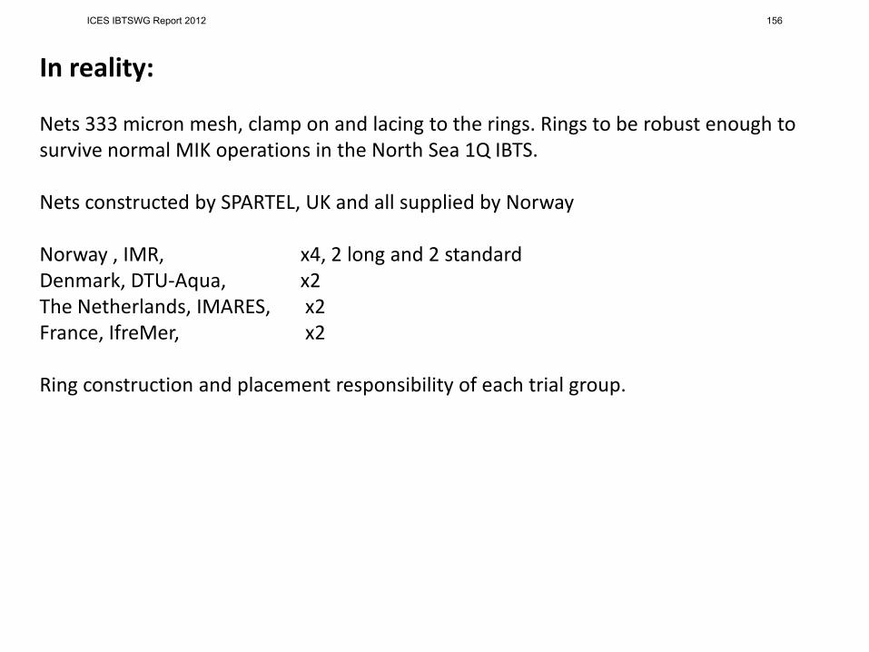
In reality: Nets 333 micron mesh, clamp on and lacing to the rings. Rings to be robust enough to survive normal MIK operations in the North Sea 1Q IBTS. Nets constructed by SPARTEL, UK and all supplied by Norway Norway , IMR, x4, 2 long and 2 standard Denmark, DTU-Aqua, x2 The Netherlands, IMARES, x2 France, IfreMer, x2 Ring construction and placement responsibility of each trial group.

ICES IBTSWG Report 2012 156

IfreMer

ICES IBTSWG Report 2012 157

ICES IBTSWG Report 2012 158

Danish setup From Peter Munk (DTU-Aqua This appeared to be no problem in our setup with fouling the nets, but it is suggested that the mounting on the ring should be changed, while there could be some damage to the big net when lowered to the deck. See the enclosed pictures for illustration of how it works. The crew were reasonably happy with the gear, and believed it would be possible to use routinely. We made comparative hauls, with and without the Mickey, these have to be processed, however a quick look at samples showed no sign of differences in catchability. I will come up with full interpretation later.

ICES IBTSWG Report 2012 159

IMARES y = 0,8011x + 0,0333 R² = 0,852

0

5

10

15

20

0 5 10 15 20

Net

B

Net A

Eggs (Nos per cub m)

y = 0,8848x - 0,0024 R² = 0,9138

0,0 0,2 0,4 0,6 0,8 1,0 1,2 1,4 1,6 1,8

0,0 0,5 1,0 1,5

Net

B

Net A

Clupeoid larvae (Nos per cub m)

0

5

10

15

20

25

20 30 40 50 60 70 80 90 100 110 120 130 Volumes filtered (cub m)

ICES IBTSWG Report 2012 160

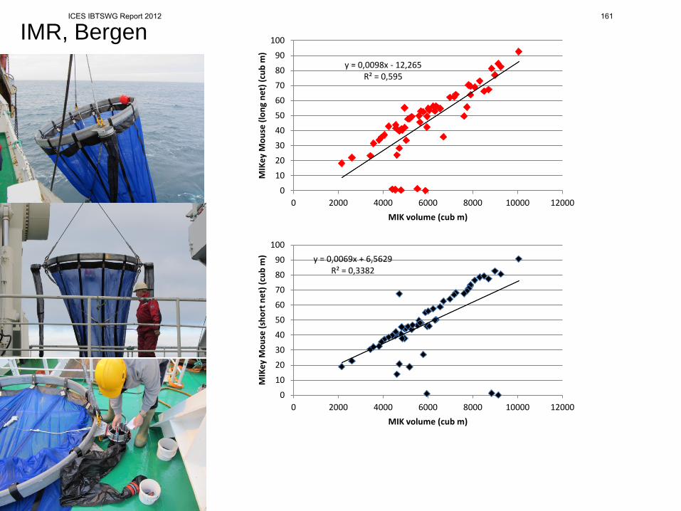
IMR, Bergen y = 0,0098x - 12,265

R² = 0,595

0

10

20

30

40

50

60

70

80

90

100

0 2000 4000 6000 8000 10000 12000

MIK

ey M

ouse

(lon

g ne

t) (c

ub m

)

MIK volume (cub m)

y = 0,0069x + 6,5629 R² = 0,3382

0

10

20

30

40

50

60

70

80

90

100

0 2000 4000 6000 8000 10000 12000

MIK

ey M

ouse

(sho

rt n

et) (

cub

m)

MIK volume (cub m)

ICES IBTSWG Report 2012 161

y = 0,4127x + 26,314 R² = 0,1514

0

10

20

30

40

50

60

70

80

90

100

0 20 40 60 80 100

MIK

ey M

ouse

(lon

g ne

t) (c

ub m

)

MIKey Mouse (short net) (cub m)

All data

y = 0,6822x + 15,294 R² = 0,6673

0

10

20

30

40

50

60

70

80

90

100

0 20 40 60 80 100

MIK

ey M

ouse

(lon

g ne

t) (c

ub m

)

MIKey Mouse (short net) (cub m)

Valid meter readings

ICES IBTSWG Report 2012 162

ICES IBTSWG Report 2012 163

The End/Begining?

2009 output (some)

ICES IBTSWG Report 2012 164

ICES IBTSWG Report 2012 165

Figure 4. The distribution of Norway pout (Trisopterus esmarkii) a. Adults (age 2+) and b. Stage I eggs in the northern North Sea in January/March 2009. Size of the dot reflects the abundance on a logarithmic scale. Black dots represent a complete absence.

ICES IBTSWG Report 2012 166

Working Document 2 ICES Benchmark Workshop on Roundfish (WKROUND 2012)

A proposed combined groundfish survey index for Cod (Gadus morhua) in the Celtic Sea ICES Area VIIe-k

By

David Stokes Marine Institute, Rinville, Oranmore, Co Galway, Ireland

Introduction Management of cod in the Celtic Sea (ICES VIIe-k) has been problematic for some time, largely related to poor information around discarding and high-grading practices in recent years. No analytical assessment was performed between 2008 and 2009 and only an exploratory assessments in 2010 - 2011. Two of the surveys used as tuning fleets in the assessment provide virtually total coverage of the VIIe-k assessment area. The French EVHOE survey covers the area from the southern Bay of Biscay up to the Irish south coast. The Irish Groundfish Survey (IGFS) extends from the Irish south coast to cover VIIg & j north, as well as VIIb in the west, included in the TAC area (Fig. 1). The current time series extends back to 2003 for the IGFS and from 1997 for the EVHOE survey. Given the shortcomings in commercial data for this stock, the intention here is to evaluate whether a combined index of IGFS and EVHOE survey data provided a more precise index as well as just improved coverage.

ICES IBTSWG Report 2012 167

Fig 1. Survey haul distribution for the French EVHOE survey and the Irish Groundfish Survey (IGFS for ICES Area VII) between 2003 – 2010. Survey data overview Both surveys are coordinated by the International Bottom Trawl Working Group (IBTS) at ICES, and therefore operate under agreed sampling protocols (ICES, 2010). In broad terms, both vessels use a GOV high headline demersal trawl towed at 4 knots for 30min to acquire the catch. Catches are carried out during daylight only and fish from each haul are sorted and sampled at sea. Catch numbers at age (CNAA) and length frequency (LF) data for EVHOE was sourced through the ICES survey database, DATRAS, and all data is standardised to numbers per hour. For IGFS data ALK’s were applied by strata to the standardised length frequencies to generate the CNAA data. Length frequencies for the surveys show a reasonably similar distribution (Fig 2a-b), although the IGFS has a tendency to catch more smaller fish than the EVHOE.

ICES IBTSWG Report 2012 168

0

10

20

30

40

50

60

70

80

90

14 20 26 31 36 41 46 51 56 61 66 71 76 81 86 91 96 102

EVHOEIGFS

Fig 2a. Total length frequency 2003 – 2010 for the EVHOE Survey (n= 1054) and the IGFS Survey (n= 1598).

0

10

20

30

40

50

60

16 26 31 36 41 46 51 58 63 69 74 91

EVHOEIGFS

Fig 2b. IGFS (n=392) vs EVHOE (n=115) LF’s for 2010. Limited amounts of cod are landed on the Irish survey in VIIb, so length frequencies are further compared just between the catches in the area of overlap VIIg,j and further to the south in VIIh on the EVHOE survey. Lengths predictably look similar within VIIg,j between the IGFS & northern EVEHOE (Fig 3). As can be seen in Fig 4, only the northern part of the EVHOE encounters smaller fish and a within year comparison for all three survey components in 2010 is given in Fig 5.

0

10

20

30

40

50

60

70

80

90

14 20 26 31 36 41 46 51 56 61 66 71 76 82 87 92 97 103

FRA_NIRL

ICES IBTSWG Report 2012 169

Fig 3. Lfs for 2003 – 2010 between IGFS (n=1598) and EVHOE (n=735) northern component (north of 50 deg Lat).

0

5

10

15

20

25

30

35

40

45

50

25 31 36 41 46 51 58 64 69 74 79 84 89 94 102

FRA_NFRA_S

Fig 4. Total length frequency for cod 2003 – 2010 for the northern EVHOE (FRA_N > 50deg Lat) and southern EVHOE (FRA_S < 50deg Lat) components of the EVHOE survey in the Celtic Sea. [FRA_N n=735; FRA_S n=319].

0

10

20

30

40

50

60

16 26 31 36 41 46 51 58 63 69 74 91

FRA_NFRA_SIRL

Fig 5. IGFS (n=392), EVHOE north (n=82) and EVHOE south (n=33) LF’s for 2010. To see how the size distributions convert to a numbers at age distribution the catch at age for the time series of both surveys was plotted for age years 0-5+ (Fig 6.). The greatest density of younger fish tend to aggregate in northern and coastal VIIg, with distribution extending further south with increasing age.

ICES IBTSWG Report 2012 170

0-group 1-group

2-group 3-group

4-group 5-group Fig 6. Plot of cod catches by age for IGFS and EVHOE survey time series (2003 – 2010) in No/Hr for each year. Combining survey indices Given both surveys historically cover different areas and employ a stratified design, it is reasonable to expect that haul allocation (survey effort) will vary between them for a given area. In combining the two data sets it is important to minimise bias whereby a survey might contribute proportionately more of one size class, for example, because it happens to have more stations in one part of the stock. With a consistent survey design this is not a problem within a survey series. However, where surveys bring different sampling distributions together the area of overlap in particular needs to be adjusted to down weight the resulting increase in effort for the combined area. A simple way to achieve this is to divide the survey area into a series of grid cells. Subsequently a mean value for each cell can be achieved across all survey point data within each grid cell. This ensures each haul only influences its localised grid cell area regardless of how many/few hauls are done in that cell. It also avoids formal

ICES IBTSWG Report 2012 171

fitting of a spatial model which can be problematic with the patchy distributions common in fisheries data sets. Station positions for both surveys for the comparable time period, 2003-2010, were used. Grid resolution was constructed so as to maximise the number of cells with information by finding the average max distance between paired hauls across years. Within the area of overlap this averaged 0.2 degrees of latitude, whereas for the entire survey area the average max distance was 0.5 deg (Table 1.). Table 1. Max and mean distances in degrees latitude between hauls for IGFS and EVHOE surveys by year. Distances are calculated for both the area of survey overlap as well as full survey extent for both surveys. On average a 0.5 degree grid will ensure haul information in each cell covering the full area for both surveys.

The catch data was plotted on a 0.5 degree grid in ArcGIS and cells relating to the area of survey overlap selected to a produce a final grid for the Celtic Sea Combined North grid (CCN grid). Figure 7 shows the CCN grid in relation to non zero cod catches for the time series of both surveys.

ICES IBTSWG Report 2012 172

Fig 7.Non zero cod catches for both surveys 2003 – 2010. Also shown is the final 0.5 degree grid used to combine surveys in the area of overlap only CCN grid (Celtic Sea Combined North grid). Number at age for each survey haul for in the data set was then allocated to the appropriate grid cell via a spatial join. The mean number at age for both surveys, including zero hauls, could then be calculated for any age and year combination for any grid cell. These are then summed across the grid to produce an annual combined index. Fig 8 shows an example of mean No/Hr 2yr old cod for the combined surveys. The same approach is applied to combine survey data for the full extent of both surveys and again an example of 2 year old cod for 2010 is presented in Fig 9.

ICES IBTSWG Report 2012 173

Fig 8. Mean number of 2yr old cod across IGFS and EVHOE surveys, per hour, for 2010. Area of overlap only.

Fig 9. Mean number of 2yr old cod across IGFS and EVHOE surveys, per hour, for 2010. Full survey extent.

ICES IBTSWG Report 2012 174

Results The combined index for the IGFS and EVHOE surveys is given in Table 2., with an extended index including derived from the full grid presented in Table 3. Exploratory analysis of the overlap area CCN grid index showed improvements over the original independent indices. Standard exploratory plots for the CNN grid are presented in Fig 10a-e with plots for the independent indices given in Fig 11a-e and 12a-e for EVHOE and IGFS respectively. Catch curves for the combined index is demonstrably more stable and internal consistency for cohorts up to age 4 are positive compared to either of the independent indices. The improvements breaks down somewhat when the full index is examined Fig 13. Catch curves become more unstable and even hooked and we loose an age class with the lack of internal consistency between 3-4 year olds seen in the scatterplot (Fig 13d). Whether this is an artefact of a relatively small and noisy dataset or whether there is some biological/stock structure that introduces noise when the VIIh data is added is not clear. The absence of juveniles in the VIIh area of the survey at any point between 2003-2010 suggests spatial structuring in quarter 4 at some level. Table 2. Combined index for IGFS and EVHOE cod in survey overlap area (CNN grid). Number per hour.

Table 3. Combined index for IGFS and EVHOE cod in VIIe-k using the full 0.5 deg grid. Number per hour.

ICES IBTSWG Report 2012 175

Fig 10a-e. Exploratory plots for combined IGFS and EVHOE survey indices for the overlapping survey area – CNN grid. Figs a-b show the log standardised indices by year and by year class and both show the relatively strong 2010 year class. Mortality curves are very stable (c)and cohort tracking from ages 1-4 is good (d). Bubble plots of proportions at age show some, but weak indication of the 2010 year class, and remnants of the earlier 2000 recruitment (e).

ICES IBTSWG Report 2012 176

Fig 11. EVHOE exploratory plots from Surba 3.0 . Log mean standardised index for ages 1-6 by year (a) and year-class (b). Catch curves (c) and scatterplots (d). Proportions by age are given in Fig E.

ICES IBTSWG Report 2012 177

Fig 12. IGFS exploratory plots from Surba 3.0 . Log mean standardised index for ages 1-5 by year (a) and year-class (b). Catch curves (c) and scatterplots (d). Proportions by age are given in Fig E.

ICES IBTSWG Report 2012 178

Fig 13. Combined index for IGFS and EVHOE for full survey area. Exploratory plots from Surba 3.0 . Log mean standardised index for ages 1-6 by year (a) and year-class (b). Catch curves (c) and scatterplots (d). Proportions by age are given in Fig E. References ICES, 2010. ADDENDUM 2: Manual for the International Bottom Trawl Surveys in the Western and Southern Areas. Revision VIII. Addendum to ICES CM 2002/D:03. In: ICESs (Ed.), Lisbon.

ICES IBTSWG Report 2012 179

Proposal of an ecosystem survey in the western English Channel

(CAMANOC)

Within IFREMER, survey proposal has to be made 2 years in advance for logistic purposes

Could this survey be part of the WGIBTS ?

Morgane Travers, Sandrine Vaz, Nicolas Desroy, Yves Vérin

ICES IBTSWG Report 2012 180

Lack of data in the western Channel

35

40

45

50

55

60

15 10 5 0

15 10 5 0

35

40

45

50

55

60

LEGEND

SURVEYS:NS-IBTS-Q3SCOGFSIGFSNIGFS_Q4CEFAS_ASP_PorcCEFAS_BFR-EVHOEFR-CGFSSP_NorthPT-GFSSP_GC

Stations Sam

Spatial coverage of international surveys targeting ichtyofauna

A particular ecosystem linking the Atlantic Ocean and North Sea with : • Strong tidal currents • Strong physical diversity (depth, bottom types,

oceanic and terrestrial influences…)

• Only old knowledge of benthic communities (from 1970s)

• No GOV ‘scientific’ data available on fish, but area where important catch are made by several countries

depth sediment

ICES IBTSWG Report 2012 181

Objectives of the survey

To characterize the state of whole ecosystem for the western English

Channel and monitor its evolution in the following years

It will be used to identify the key components of this ecosystem, to

understand its functioning, and analyze its evolution under environmental

and anthropogenic pressures.

To do so, all biological compartments need to be sampled (benthos, fish

plankton, top predators) and the abiotic environment has to be characterized.

First year survey planned in September for zooplankton and larval bloom

and fish abundance (large commercial catch at this season) – IBTS protocol

ICES IBTSWG Report 2012 182

Sampling the benthic community Using a combination of gears, the sampling of benthos will address 3 objectives : • To precise the geomorphology of the bottom (sedimentology) and the EUNIS typology • To characterize the spatial coverage of benthic species in the western Channel

-> systematic sampling • To evaluate the evolution of benthos in the past 40 years (comparison with the

distribution limits observed in the 1970s for species of interest, and analysis of possible link with environmental changes) -> samples along 2 transects

• Ralier du Baty dredge • Hamon grab • Megafauna sampled in

GOV • Under water videos

ICES IBTSWG Report 2012 183

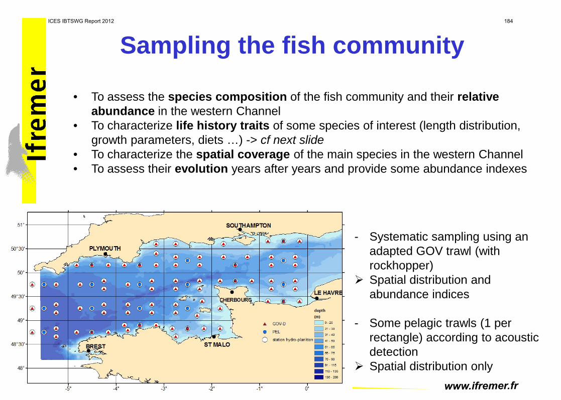
Sampling the fish community

• To assess the species composition of the fish community and their relative abundance in the western Channel

• To characterize life history traits of some species of interest (length distribution, growth parameters, diets …) -> cf next slide

• To characterize the spatial coverage of the main species in the western Channel • To assess their evolution years after years and provide some abundance indexes

- Systematic sampling using an adapted GOV trawl (with rockhopper)

Spatial distribution and abundance indices

- Some pelagic trawls (1 per

rectangle) according to acoustic detection

Spatial distribution only

ICES IBTSWG Report 2012 184

Details on fish species of interest (DCF)

Benthic invert.

Cepha-lopods

Benthic fish

Demersal fish

Pelagic fish*

Catch in september (2000-2008)

in western channel anchovy

seabass

monkfish

Horse mackerel

Conger Haddock

Black seabream

Red gurnard

Herring

Pollack

Ling

Whiting

Cod

Small spotted catshark Rays

Red mullet

John Dory

Sardine

Pouting

For these species, data collection for :

- Size spectrum

- Relation between size, age, maturity

- Stomac content / trophic level

Sprat

Sole Plaice

*Proportion of pelagic fish is underestimated

ICES IBTSWG Report 2012 185

Sampling the plankton and abiotic environment

• To characterize the abiotic environment, needed to derived habitat preferences of living components

• To evaluate the importance of primary production through phytoplankton abundance and distribution

• To characterize the spatial distribution, the taxonomic composition and the length distribution of the secondary production (zooplankton)

• To locate and estimate the importance of spawning and nursery areas (eggs and larvae of fish)

Systematic sampling at trawling locations: - CTD + LOPC - CUFES (eggs pump) - Niskin bottle - Zooplankton net - Ichthyoplankton net (larval index) - Acoustic (continuously, for

bathymetry, pelagic fish, zooplankton biomass)

ICES IBTSWG Report 2012 186

Observation of top predators and « food web sampling »

• To estimate the relative abundance and spatial distribution of the top predators: marine mammals and birds (providing data to larger groups within the context of Natura 2000)

- Continuous observation during daylight

• To understand the food web dynamics by evaluating the links between predators (mostly fish species of interest) and prey (other fish, ichtyoplankton, zooplankton, phytoplankton, benthos).

- Sampling and preserving individuals from plankton nets and trawls, to be analyzed latter at lab (possibly through morphology, stomach content, stable isotopes, fatty acids…)

ICES IBTSWG Report 2012 187

Some details

• Proposal to be (re)submitted in September 2012, following the IBTS sampling protocol

• 1st “complete” survey planned for September 2014 (Q3) : 30 days, all components of the ecosystem will be assessed - > reference point of the ecosystem state

• Every October (Q4) there will be an annual survey: 15 days, it will not include such sampling effort for benthos (only megafauna from the trawl) and will not include pelagic trawl

• Indices derived from this annual survey may be used in the MSFD, for biological measurement of DCF fish, and as time series develop, they could be used for fish abundance indices in the 7E area for ICES WG.

ICES IBTSWG Report 2012 188

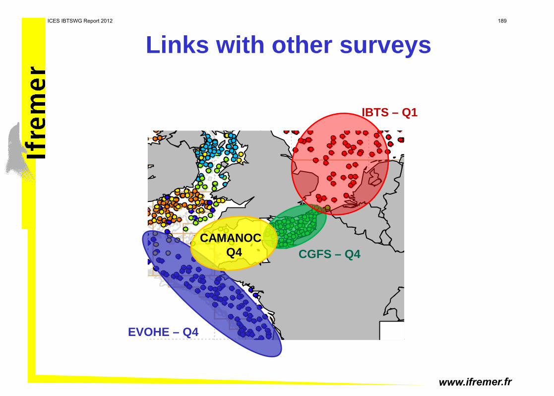
Links with other surveys

EVOHE – Q4

CGFS – Q4

IBTS – Q1

CAMANOC Q4

ICES IBTSWG Report 2012 189

| 1

Changes to the Q1 + Q4 Scottish VIa.IBTS and Q3 Scottish VIb.IBTS

Andrzej Jaworski, Finlay Burns and Rob Kynoch ,jaworskia@marlab.ac.uk, burnsf@marlab.ac.uk, kynochr@marlab.ac.uk

Introduction The Q1 Scottish VIa IBTS survey has been running since 1981 and up until 2010 this was performed using a repeat station format with the GOV survey trawl together with the west coast groundgear ‘C’ rig,. Similarly the Q4 Scottish VIa IBTS and Q3 Scottish VIb.IBTS (Rockall haddock) have been running in their present form since 1990 and 1999 respectively, once again using the GOV survey trawl with groundgear ‘C’ and the fixed station format. 2011 heralded the start of a new randomised stratified survey design in both these areas replacing the previous repeat station survey format consisting of the same series of survey trawl positions being sampled at approximately the same temporal period every year. A move towards some sort of random stratified survey design was therefore judged necessary. The largest obstacle preventing an earlier move to a more randomised survey design was the lack of confidence in the ‘C’ rig to tackle the potentially hard substrates that a new randomised survey was likely to encounter in both these areas. The first step in the process of modifying the survey was therefore to design a new groundgear that would be capable of tackling such challenging terrain. The modifications made to the trawl configuration are thus summarised below. Groundgear All three surveys were undertaken using the standard GOV research trawl but with a modified groundgear more suited to the hard and often undulating topography encountered within ICES subareas VIa and VIb. This gear consisted of 530mm, 450mm and 350mm rubber wheel bobbins with 15m x 150mm rubber leg sections along each wing. Despite the large bobbins present in the ‘C’ rig it consistently failed to provide adequate protection to the trawl on harder ground – especially in the wing sections - and in 2006 the search began to find a new replacement rockhopper rig for the west coast - groundgear ‘D’. The configuration selected was that already being used by Ireland in VIa during their quarter 4 groundfish survey and consists of 400mm hoppers discs in the centre reducing to 350mm discs at the quarters and then 300mm discs out to the wingends. Instead of being attached to the groundgear using toggle chains – as was the case with ‘C’ - the footrope is lashed directly to the groundgear using a series of steel rings. This gear has been used during a number of gear trials and throughout has proved robust and reliable. See figure 1. Wire Sweep Rig The Rockall survey is conducted exclusively in depths greater than 100m whereas on the Scottish West Coast surveys approximately 80% of tows are

ICES IBTSWG Report 2012 190

| 2

made in depths deeper than 80m. Historically, only 60m sweeps were used throughout, during all Scottish western surveys, despite the IBTS recommendation that for trawls conducted in depths deeper than 70m that the 110m sweep rig be used. From 2011, the new configuration - in an effort to maintain net geometry parameters (wingend spread & headline height) and ground gear bottom contact – will utilise both 60m and 110m sweep rigs. Although the IBTS recommends 70m as the cutoff for changing the sweep length the new survey will aim to standardise with the current Irish Groundfish survey and adopt the cut off for deploying the long sweep rig on trawls in depths in excess of 80m in both ICES subareas VIa and VIb. GOV Trawl No modifications have been made to the GOV trawl frame ropes nor the mesh sizes used in the different netting panel sections. The only alteration from the previous trawl design is the incorporation of tearing strips and guard meshes constructed from 5mm high tenacity double braided polyethylene twine. The mesh sizes of the double netting panels corresponded to the mesh sizes being replaced. To maintain consistency with the old netting the overall dimensions of the double netting panels, tearing strips and guard panels were determined by stretched length and not mesh counts. Double netting has also been inserted into upper/lower wing tips, 6 mesh deep guard inserted into upper/lower 1st wing sections, 1st belly section, 2nd belly section tearing strip and 5 mesh deep headline guard. See figure 1. This strengthening of the netting in the panels around the fishing line coupled with the other modifications made to both groundgear and sweep rig afford the GOV the best possible chance of being able to complete a comprehensively stratified and random bottom trawl survey that will aim to sample all fishable areas within ICES Subarea VIa/VIb. Figure 1. GOV lower wingend showing 5mm double PE guard netting and Ground gear D hoppers

ICES IBTSWG Report 2012 191

| 3

MSS West Coast, and Rockall Survey designs

ICES Subarea VIa, West Coast Q1 and Q4 surveys

Stratification

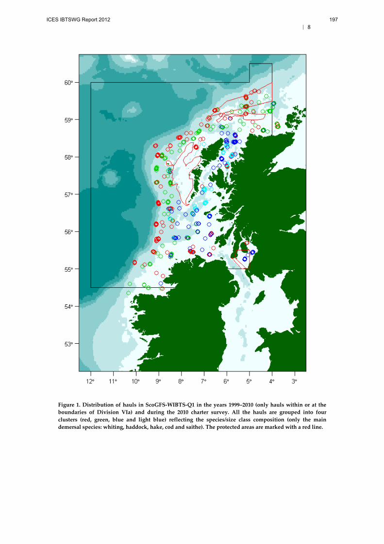
ScoGFS-WIBTS-Q1 is primarily a juvenile gadoid survey. In the design phase for this survey, the focus was on demersal species: cod, haddock, whiting, saithe and hake. Abundance data for these species in the period 1999–2010 were analysed. In addition, data from a charter survey which was conducted in the first quarter of 2010 were analysed (however, no hake data were available for this survey). This gadoid survey was completed on charter vessels using a non-standard rockhopper gear and was intended to complement the ScoGFS-WIBTS-Q1 survey carried out within the same temporal period and geographical area. Similar to the ScoGFS-WIBTS-Q1 survey, the design of ScoGFS-WIBTS-Q4 was aimed at using data for the five main demersal species. In this case, data for the period 1996–2010 were used. All fish densities in either ScoGFS-WIBTS-Q1 (complemented with the 2010 charter data) or in ScoGFS-WIBTS-Q4 were standardised (they were given as log numbers per 30 minutes). To account for year-to-year differences in abundance, these densities were then expressed in relation to the average density for a given species/size group and in a given survey/year. As a result, maps of average distribution could be generated for the five demersal species based on the historical data. Tentative K-means clustering of density data was carried out with four clusters, separately for each of the two surveys. The resulting clusters for ScoGFS-WIBTS-Q1 are shown in Figure 1. Species/size class composition for each cluster is displayed in the barplot in Figure 2. A brief description of the four clusters follows (see also species/size class composition by haul in Figure 3): Cluster 1 (red): generally deeper waters, much less small fish (particularly whiting), a bit of medium/big fish (mainly hake). Cluster 2 (green): more fish than in Cluster 1 (mainly whiting and haddock), but small fish are still less than the average. Cluster 3 (blue): more small fish (particularly whiting), less big fish. Cluster 4 (light blue): more small whiting (but less than in Cluster 3), considerably less haddock and markedly more hake (small/medium) than in other strata. The inverse distance weighting (IDW) was used to interpolate fish density at any position in the 2’×2’ grid. In this method, estimates of an attribute are made based on values at nearby locations weighted by distance from the interpolation location. The weights λi are given by

ICES IBTSWG Report 2012 192

| 4

∑=

= n

i

pi

pi

i

d

d

1

1

1λ

where di is the distance between x0 (interpolation location) and xi, p is a power parameter and n is the number of sampled points used for the estimation (Shepard, 1968). With the present data, the choice of power parameter and neighbourhood size was based on the results of cross-validation. In this procedure, each haul was excluded in turn to determine how accurate the prediction was, given the remaining observations. Some optimal values for the minimum distance and for the parameter p in IDW could thus be determined, which minimised the error of prediction. These values were used to calculate the mean density for each cell in the grid. Subsequently, K-means clustering was applied to all grid cells (except those in the protected areas shown in Figure 1), again with four clusters as a result. The optimal parameter values from the cross-validation were not very effective here as they tended to generate patchy/irregular shapes, which was undesirable for the purpose of stratification. However, choosing some sub-optimal values resulted in satisfactorily smooth shapes. The selected values for these parameters were 25 nm for the minimum distance and 0.80 for the power parameter p. These could be interpreted roughly as the maximum distance over which an individual sample is allowed to influence the surrounding ones and as an indication of smooth peaks (with 0 < p < 1) over the interpolated points. The final strata separation for ScoGFS-WIBTS-Q1 is shown in Figure 4.

Allocation of sampling effort In the process of effort allocation, each individual polygon in Figure 4 was treated separately (for instance “red1”, “red2” and “red3” rather than just “red”) and all these polygons are further referred to as “strata”. To maximise the precision of the fish density estimate for the total survey area, survey effort was allocated among strata in such a way that the proportion of the samples in each stratum (ni/n) was given by

∑=

= S

iii

iii

sA

sAnn

1

where Ai = area (m2) of stratum i, si = standard deviation within stratum i, S = number of strata (Gunderson, 1993). Thus, more sampling effort was allocated to bigger strata and those with a higher within-stratum variance. The selection of stations was carried out randomly in each stratum (given the number of hauls per stratum), and with the constraint that the minimum distance between two nearest stations was less than 10 nm. This ensured that (a) each possible sample point had an equal chance of being selected; and (b) that there was an even coverage of samples throughout the strata (avoiding clustering of samples and concomitant large open spaces without samples).

ICES IBTSWG Report 2012 193

| 5

ICES Subarea VIb, Rockall Haddock survey – Q3

Stratification

The ScoGFS-Q3 Scottish VIb.IBTS is primarily a juvenile haddock survey. After completing the survey in 2009, it was recognised that there was a need to include areas with high haddock densities not covered by the survey. Those high densities were found in deeper waters during the monkfish survey in quarter 2 in the Rockall area. Since apparently some significant parts of the stock were not sampled during the haddock survey, the resulting abundance index were likely to have been biased. Figure 5 shows the recorded haddock numbers per 30 minutes trawling by size class vs. depth, in the haddock and monkfish surveys in 2009. From the maps with the monkfish survey (Figure 6), it can be seen that there were significant haddock numbers beyond the 200 m isobath, in a few cases, even beyond 300 m. For many age groups in the haddock survey, the 200–240 m depth was clearly not the upper limit of their distribution. The precision of the survey was increased through stratification. With haddock being caught between 140 and 400 m, it was possible to divide the fished area into depth strata. To keep the density homogenous and the intra-stratum variance low, five strata were selected based on depth. The upper limit of the last stratum was first set to 470 m (Figure 7), but this is likely to be reviewed as the survey progresses.

Allocation of sampling effort With regard to how to allocate sampling effort between strata, the information from previous surveys were of limited value as the distribution of haddock (of different age groups) at Rockall is not exactly the same every year. Initially, equal (or almost equal) number of hauls to each stratum were considered. With about 40 hauls per trip (as has been the case in the previous Rockall haddock surveys), it would have been possible to allocate eight hauls to each stratum with five strata. However, it was agreed that there was enough information to avoid allocating the same number of samples to each stratum and that one should use approximate multiples of sampling intensity allocated according to abundance in each stratum. As estimated from the existing survey data and also the Rockall monkfish survey data. Sampling intensity was thus modified with k samples per unit area in low density strata, k*2 samples per unit area in medium density strata and k*3 in high. The proportion of the samples in each stratum (ni/n) was given by

∑=

= S

iii

iii

mA

mAnn

1

where Ai = area (m2) of stratum i, mi = number samples per unit area within stratum i (with m1= 1, m2= 2, m3= 3, m4= 2, m5= 1), S = number of strata. After considering the data available, it was agreed that:

• Sampling should be split across five depth strata

• Overall sampling total should reflect previous coverage

ICES IBTSWG Report 2012 194

| 6

• Sampling intensity per stratum should reflect the density of fish in each stratum

• Within strata, the samples were chosen at random within strips of equal area. This ensures that (a) each possible sample point has an equal chance of being selected; and (b) that there is an even coverage of samples throughout the strata (avoiding clustering of samples and concomitant large open spaces without samples).

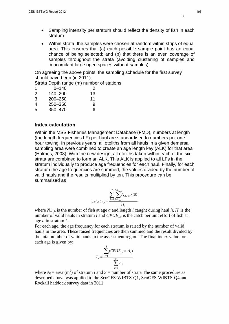
On agreeing the above points, the sampling schedule for the first survey should have been (in 2011): Strata Depth range (m) number of stations 1 0–140 2 2 140–200 13 3 200–250 11 4 250–350 9 5 350–470 6

Index calculation Within the MSS Fisheries Management Database (FMD), numbers at length (the length frequencies LF) per haul are standardised to numbers per one hour towing. In previous years, all otoliths from all hauls in a given demersal sampling area were combined to create an age length key (ALK) for that area (Holmes, 2008). With the new design, all otoliths taken within each of the six strata are combined to form an ALK. This ALK is applied to all LFs in the stratum individually to produce age frequencies for each haul. Finally, for each stratum the age frequencies are summed, the values divided by the number of valid hauls and the results multiplied by ten. This procedure can be summarised as

i

H

h

ll

llhla

ai H

N

CPUE

i

∑∑=

=

=

×

= 1,,

,

max

min

10

where Na,l,h is the number of fish at age a and length l caught during haul h, Hi is the number of valid hauls in stratum i and CPUEi,a is the catch per unit effort of fish at age a in stratum i. For each age, the age frequency for each stratum is raised by the number of valid hauls in the area. These raised frequencies are then summed and the result divided by the total number of valid hauls in the assessment region. The final index value for each age is given by:

∑

∑

=

=

×

= S

ii

S

iiai

a

A

ACPUEI

1

1, )(

where Ai = area (m2) of stratum i and S = number of strata The same procedure as described above was applied to the ScoGFS-WIBTS-Q1, ScoGFS-WIBTS-Q4 and Rockall haddock survey data in 2011

ICES IBTSWG Report 2012 195

| 7

References Gunderson, D. R. 1993. Surveys of Fisheries Resources. John Wiley & Sons, Inc. New York,

248 pp.

Holmes, S. J. 2008. ROAME MF0170: Alternative Survey Index Estimation. FRS Production of Scottish West Coast Survey Indices. Fisheries Research Services Internal Report No 10/08.

Shepard, D. 1968. A two-dimensional interpolation function for irregularly-spaced data. Proceedings of the 1968 ACM National Conference, 517–524.

ICES IBTSWG Report 2012 196

| 8

Figure 1. Distribution of hauls in ScoGFS-WIBTS-Q1 in the years 1999–2010 (only hauls within or at the boundaries of Division VIa) and during the 2010 charter survey. All the hauls are grouped into four clusters (red, green, blue and light blue) reflecting the species/size class composition (only the main demersal species: whiting, haddock, hake, cod and saithe). The protected areas are marked with a red line.

ICES IBTSWG Report 2012 197

| 9

Figure 2. Species/size class abundance by cluster.

ICES IBTSWG Report 2012 198

| 10

Figure 3. Species/size class abundance by haul and cluster (with low abundances in blue and high abundances in red).

ICES IBTSWG Report 2012 199

| 11

Figure 4. Allocation of sampling effort among strata with the optimised route for ScoGFS-WIBTS-Q1 in 2011.

ICES IBTSWG Report 2012 200

| 12

140 160 180 200 220

0

1

2

3

4 0 10 cm

140 160 180 200 220

0.0

0.5

1.0

1.5

2.0 10 20 cm

140 160 180 200 220

0123456 20 30 cm

140 160 180 200 220

0

2

4

6

8 30 40 cm

140 160 180 200 220

0

1

2

3

4

5 40 50 cm

140 160 180 200 220

0.0

0.5

1.0

1.550 60 cm

140 160 180 200 220

0.00.20.40.60.81.01.21.4 60 cm

140 160 180 200 220

0

2

4

6

8 All sizes

Rockall haddock survey 2009

Depth (m)

Had

dock

log

num

ber p

er s

tand

ard

tow

200 300 400 500 600 700

0123456 0 10 cm

200 300 400 500 600 700

0123456 10 20 cm

200 300 400 500 600 700

0

2

4

6

8 20 30 cm

200 300 400 500 600 700

0

2

4

6

8 30 40 cm

200 300 400 500 600 700

0

1

2

3

4

5 40 50 cm

200 300 400 500 600 700

0.0

0.5

1.0

1.5

2.0

2.5

3.0 50 60 cm

200 300 400 500 600 700

0.0

0.5

1.0

1.5 60 cm

200 300 400 500 600 700

0

2

4

6

8

10All sizes

Rockall monkfish survey 2009

Depth (m)

Had

dock

log

num

ber p

er s

tand

ard

tow

Figure 5. Haddock abundance (number per standard haul of 30 minutes) by size class vs. depth in the Rockall haddock survey (upper panel) and in the Rockall monkfish survey (lower panel) in 2009.

ICES IBTSWG Report 2012 201

| 13

Figure 6. Haddock distribution (number per standard haul of 30 minutes) by size class in the Rockall haddock survey in 2005–2009 (upper panel) and in the Rockall monkfish survey in 2006–2009 (lower panel). The Rockall haddock box is shown as a red rectangle. The EU boundary is marked with a dash line.

ICES IBTSWG Report 2012 202

| 14

Figure 7. Five strata in the new Rockall survey design.

ICES IBTSWG Report 2012 203

| 15

Figure 8. Protected areas on the Rockall Bank.

-18 -16 -14 -12 -10 -8 -6 -4 -2 055

55.5

56

56.5

57

57.5

58

58.5

59

Latit

ude

longitude

NW Rockall

SW Rockall

W Rockall Mound

Logachev mounds

Kevins corner

ICES IBTSWG Report 2012 204

Catch comparison trials to assess the effect of a rockhopper ground gear on the catches of the Scottish GOV survey trawl.

By

RJ Kynoch, F Burns & A Edridge

Materials & Methods

Sea trials Two comparative surveys were carried out on Marine Scotland Science (MSS) survey vessel FRV Scotia (LOA 68.6m). This is the standard survey platform used by Scotland to conduct its annual International Bottom Trawl Surveys (IBTS). The first of these was completed during May 2006 and was undertaken exclusively on the Rockall plateau in ICES Subarea VIb. The second survey ran from 23 October until 3 November 2009 with hauls being completed around the Shetland and Orkney Islands in ICES Subarea IVa. Trawl depths encountered during the first comparative survey at Rockall ranged from 137m to 191m and during the second survey the depth range was 69m to 140m. Scanmar acoustic instrumentation was used during every haul to check gear geometry and a self-recording sensor rigged at the midpoint of the ground gear monitored bottom contact. For both surveys towing speed and warp ratios were as per standard survey protocols for Scottish IBTS surveys. Description of trawl gear Two similar GOV (Grand Opening vertical) 36/47 trawls supplied by the MSS Netstore were used during both cruises (Figure 1). One trawl was rigged with a 45.7m bobbin ground gear (C rig) which has been the standard groundgear for Scottish surveys covering ICES Areas VIa and VIb since 1985. The ground gear incorporates rubber wheel bobbins in the bosom/quarter sections and then 3 x 5m rubber disc sections out the wingends (Figure 2). The other trawl was rigged with the new rockhopper ground gear (D rig), which incorporates rockhopper disc’s along its 46m length (Figure 3). Sweepline and otterboard rig were the same for both trawls (Figure 4). Headline uplift was provided by an “Exocet” kite (0.85m x 0.85m) together with 60 x 200mm diameter plastic floats. Assuming a static uplift of 2.47kg each the floats provide a total buoyancy of 148.2kg. The trawl rigged with C rig (control) was worked from the vessels lower net drum and the other trawl with D rig (test) worked from the upper net drum.

ICES IBTSWG Report 2012 205

Figure 1 – GOV survey trawl.

ICES IBTSWG Report 2012 206

Figure 2 – Bobbin ground gear rig C.

ICES IBTSWG Report 2012 207

Figure 3 - Rockhopper ground gear rig D.

ICES IBTSWG Report 2012 208

Figure 4 – Otterboard, flotation and sweepline wire rig for D and C gears. Experimental design For the first survey at Rockall the haul procedure was the same throughout the trials and consisted of paired hauls of 30 minute duration (as per standard survey protocols). After completion of the first haul the vessel immediately steamed back to the start position (and made the second haul 50-95 minutes from knockout to block- up) down the same fishing track. To minimise bias the order of deployment was alternated so both gears were fished either first or second (CvD or DvC). During the cruise a number of paired hauls were made using the same ground gear (CvC or DvD) to assess potential differences in fish catch rates between the first and second gears due to trawl disturbance. During the second cruise in 2009 a similar paired haul procedure was followed. The time from ending the first haul and blocking up the second haul ranged from 38 to 98 minutes. Due to the limited number of days and the results obtained from the previous survey only paired hauls were made to test the difference between the two ground gear rigs (CvD and DvC), no hauls were made to test for trawl disturbance. Catch handling The catches were handled in the same consistent manner during both surveys. After each haul the total catch was sorted into individual species and then weighed. All species were then measured to the nearest 1.0 cm below. When large catches of a particular species were encountered a random sub-sample was then measured and raised to the total number caught in the codend.

ICES IBTSWG Report 2012 209

Results In 2006 a total of 50 valid paired hauls were completed of which 8 pairs were CC, 8 pairs DD, 18 pairs CD and 16 pairs DC. In 2009 there were 21 valid paired hauls completed of which 11 pairs were CD and 10 pairs DC. During both cruises a number of paired hauls had to be excluded due to damage to the trawl rigged with C rig. For clarity the test cases were labelled according to which gear was towed first and then second. Gear geometry Similar trawl vertical openings were recorded during both cruises with mean values ranging from 4.4 to 5.4m in 2006 (Tables 1 and 2) and 4.6m to 5.4m in 2009 (Table 3). Wingend and otterboard spreads were consistent between the two gears but otterboard spread was slightly lower for both in 2009 due to the shallower depths encountered compared to the previous survey. Mean speed over the ground in 2006 ranged from 3.5 to 4.1 knots and in 2009 from 3.6 to 4 knots except for one haul when the mean speed was slightly lower at 3.3 knots. As mentioned above during both cruises the C rig proved problematic with a number of hauls being discarded due to its susceptibility to sustaining damage mainly to the lower wing and belly sheet netting. It was noted that most damage had occurred along the netting attached to the 15m rubber-leg sections where it was presumed stones were being scooped into the trawl and then chaffing out through the netting. No damage was sustained during either cruise by the trawl fitted with D rig.

ICES IBTSWG Report 2012 210

Table 1 – Haul summary for paired hauls during 2006 cruise

Paired haul set

Paired haul set - First haul Paired haul set - Second haul

Ground Gear

rig

Mean water depth (m)

Warp length

(m)

Mean Headline

Height (m)

Mean Wing

Spread (m)

Mean Door

Spread (m)

Mean Speed Made Good (kits)

Ground gear rig

Mean water depth (m)

Warp length

(m)

Mean Headline

Height (m)

Mean Wing

Spread (m)

Mean Door

Spread (m)

Mean Speed Made Good (kits)

1 C 165 525 5.3 18.8 85.4 3.6 C 165 525 5.3 19.9 86.7 3.9 2 C 150 480 5.2 23.3 86.2 3.8 D 150 480 5.0 20.2 84.4 4.1 3 D 170 540 5.1 19.6 85.0 3.5 D 170 540 5.1 19.6 84.7 3.6 4 D 150 450 5.1 19.2 82.6 3.7 C 150 450 N/R 19.7 85.4 3.7 5 C 185 600 5.2 20.3 88.1 3.8 D 185 600 5.1 21.7 86.1 3.8 6 D 191 600 4.8 19.7 84.8 3.8 C 190 600 5.2 19.7 84.8 3.6 7 C 186 600 5.4 22.0 87.0 3.6 C 187 600 5.0 20.4 87.3 3.7 8 C 180 570 5.1 19.5 85.7 3.7 D 182 570 4.9 19.3 84.6 3.8 9 D 178 540 5.0 19.4 85.7 3.9 D 172 540 4.9 20 85.9 3.8

10 D 168 525 5.0 19.5 85.7 3.8 C 168 525 5.3 19.5 87.5 3.8 11 C 174 525 5.1 19.8 88.2 3.9 D 174 525 4.9 21 84.8 3.6 12 D 159 500 5.0 19.8 84.4 3.8 C 159 500 4.9 19.3 86.5 3.9 13 C 153 500 5.0 19.3 86.5 3.8 C 154 500 5.0 20.1 85.0 3.7 14 C 175 550 N/R 19.2 85.6 3.9 D 175 550 4.8 19.2 84.4 3.8 15 D 185 600 4.7 19.3 86.1 3.8 D 185 600 4.9 19.2 85.9 3.8 16 C 159 510 4.9 21.8 87.0 3.9 D 159 510 4.9 19.3 84.4 3.8 17 D 148 510 4.9 18.9 85.1 3.9 C 147 510 5.0 19.5 86.7 3.7 18 C 159 510 N/R 19.7 86.4 3.6 D 160 510 4.7 19 84.3 3.6 19 D 168 510 4.8 19.5 84.9 3.9 C 168 510 4.9 20.1 87.3 3.8 20 C 171 510 4.8 19.3 86.3 3.9 D 174 510 4.8 19.1 84.6 3.9 21 D 181 555 4.8 21.0 85.5 3.9 C 181 555 4.9 19.4 87.8 3.9 22 C 149 510 5.0 19.4 87.1 3.9 D 149 510 5.0 22 83.2 3.8 23 D 170 540 4.4 20.5 85.7 3.7 C 169 540 5.0 19.7 87.3 3.8 24 C 162 510 5.0 19.3 86.8 3.7 C 160 510 5.0 19.3 87.4 3.8 25 C 155 460 5.0 19.1 86.8 3.9 D 155 460 5.0 21.4 83.8 3.9 26 D 143 425 5.0 18.7 82.4 3.8 D 144 425 4.8 18.8 84.9 4.0

ICES IBTSWG Report 2012 211

Table 2 – Haul summary for paired hauls during 2009 cruise continued

Paired haul set

Paired haul set - First haul Paired haul set - Second haul

Ground Gear

rig

Mean water depth (m)

Warp length

(m)

Mean Headline

Height (m)

Mean Wing

Spread (m)

Mean Door

Spread (m)

Mean Speed Made Good (kits)

Ground gear rig

Mean water depth (m)

Warp length

(m)

Mean Headline

Height (m)

Mean Wing

Spread (m)

Mean Door

Spread (m)

Mean Speed Made Good (kits)

27 D 174 540 4.6 19.6 86.8 4.0 C 177 540 4.9 19.7 88.3 4.0 28 C 153 480 4.8 19.6 85.9 3.8 C 150 480 4.9 20 85.8 3.8 29 C 163 525 4.8 19.5 86.3 3.6 D 163 525 4.7 19.3 85.7 3.6 30 D 156 540 4.6 19.2 86.5 3.9 C 156 540 4.8 19.8 87.4 4.0 31 C 169 540 5.0 20.4 87.2 3.9 D 169 540 4.6 19.6 86.7 4.0 32 D 161 510 4.6 19.4 86.5 4.1 C 161 510 5.1 20.3 84.1 3.7 33 C 187 570 4.9 21.8 86.3 3.8 D 187 570 4.7 21.1 86.2 3.8 34 D 158 510 4.7 19.8 84.2 3.6 D 160 510 4.6 19.6 84.4 3.8 35 D 185 600 4.6 19.8 85.6 3.8 C 184 600 4.8 19.6 85.4 3.8 36 C 175 555 N/R 18.9 84.7 3.7 C 175 555 4.9 18.8 82.6 3.8 37 C 154 500 5.0 19.0 83.9 3.7 D 155 500 4.9 18.9 84.1 3.8 38 D 160 500 4.8 18.7 83.1 3.7 D 160 500 4.8 18.7 83.0 3.8 39 D 165 525 4.8 20.3 85.5 3.7 C 167 525 4.8 19 87.2 3.9 40 C 172 525 5.0 18.9 85.7 3.8 C 171 525 5.0 N/R 85.8 3.8 41 C 166 510 5.0 19.0 85.0 3.9 D 168 510 4.8 N/R 86.1 4.1 42 D 168 510 4.8 20.1 83.6 3.7 D 171 510 4.8 19.3 83.8 3.9 43 D 182 555 4.5 19.6 85.4 3.8 C 182 555 4.8 N/R 85.9 3.9 44 C 154 510 5.1 19.7 86.9 3.9 D 155 510 4.7 20.5 86.4 3.7 45 D 172 540 4.7 20.8 84.8 3.7 D 172 540 4.7 21.7 85.6 3.9 46 D 163 510 5.0 19.7 85.4 3.9 C 163 510 5.2 19.2 87.0 3.7 47 C 152 460 5.1 19.1 85.8 4.1 C 154 460 5.1 19.2 85.6 3.8 48 C 151 460 5.1 19.6 85.2 3.8 D 152 460 5.1 19.9 85.9 3.9 49 D 177 540 4.9 20.5 86.9 3.7 C 177 540 4.8 20.3 88.5 3.9 50 C 140 450 4.9 19.4 86.3 3.9 D 137 450 4.9 19.6 84.8 3.9

ICES IBTSWG Report 2012 212

Table 3 – Haul summary for paired hauls during 2006 cruise

Paired haul set

Paired haul set - First haul Paired haul set - Second haul

Ground Gear

rig

Mean water depth (m)

Warp length

(m)

Mean Headline

Height (m)

Mean Wing

Spread (m)

Mean Door

Spread (m)

Mean Speed Made Good (kits)

Ground gear rig

Mean water depth (m)

Warp length

(m)

Mean Headline

Height (m)

Mean Wing

Spread (m)

Mean Door

Spread (m)

Mean Speed Made Good (kits)

1 C 114 360 5.1 19.3 82.3 3.7 D 114 360 5.4 18.4 76.3 3.7 2 D 117 365 5.3 19.2 76.8 4.0 C 118 365 4.9 19.4 82.3 3.9 3 C 113 360 5.0 19.0 81.2 3.9 D 113 360 5.3 19.3 76.3 3.7 4 D 108 360 5.2 19.0 77.6 3.6 C 108 360 4.9 19.5 81.8 3.8 5 C 107 360 4.9 19.3 82.0 3.8 D 108 360 5.3 20.9 77.3 3.9 6 D 108 360 5.3 18.6 78.0 3.8 C 109 360 4.9 18.8 82.0 3.8 7 C 108 360 5.1 18.6 78.7 3.7 D 107 360 5.2 19.5 76.3 3.6 8 C 110 365 4.9 18.4 79.0 3.8 D 110 360 5.2 18.7 75.9 3.6 9 D 109 360 5.3 N/R 76.7 3.6 C 112 360 4.6 19.3 83.0 3.7

10 C 111 370 5.0 18.5 78.8 3.7 D 111 370 5.3 18.4 75.1 3.6 11 D 108 365 5.2 19.8 76.7 3.5 C 108 365 4.8 N/R 80.0 3.7 12 D 140 450 5.0 20.4 81.1 3.9 C 140 450 4.9 22.2 85.4 3.8 13 C 130 405 5.0 19.7 83.3 3.7 D 129 405 5.3 19.4 75.7 3.3 14 D 130 390 5.3 19.2 76.7 3.7 C 130 390 5.0 19.1 83.1 3.7 15 D 105 345 5.1 19.5 76.0 3.6 C 106 345 4.9 19.0 79.8 3.6 16 C 105 345 4.8 17.7 78.9 3.7 D 104 345 5.1 18.2 75.0 3.8 17 D 100 345 5.3 19.9 75.6 3.7 C 101 345 4.6 20.1 79.3 3.6 18 C 72 240 4.9 16.4 67.0 3.8 D 75 240 5.1 17.0 62.7 3.7 19 C 69 255 5.2 15.6 64.0 3.5 D 70 255 5.3 16.9 65.5 3.7 20 D 70 240 5.3 17.2 66.6 3.7 C 70 240 5.3 15.9 65.9 3.6 21 C 72 240 5.0 16.7 69.2 3.7 D 72 240 5.0 17.8 74.3 3.6

ICES IBTSWG Report 2012 213

Catch comparison data Sufficient numbers of haddock, lemon sole and megrim were encountered in 2006 and haddock and whiting in 2009 for subsequent analysis. Limited numbers of cod were encountered during the 2009 cruise but were not sufficient to allow any final analyses. The catches retained in the codends of the test and control gears were used to estimate the catch rate of test gear D relative to the control gear C. The analysis is described in the Appendix. The data was analysed over a number of stages before a direct comparison could be made between the two ground gears. In figures 5 to 8 the relative catch rates are shown as the proportion of fish retained in the test gear as compared to the control gear. A value of less than one indicates that the test gear caught fewer fish at that length and a value greater than one indicates more fish were caught in the test gear compared to the control. A dashed line indicates where the relative catch rate did not differ significantly from parity (control), whereas a solid line indicates there is point-wise significance at the 5% level. The first analysis examined whether the order that the gears were towed had a significant effect. This was achieved using the 2006 CC and DD hauls and tested the second towed gear (test) against the first (control). No significant differences in the relative catch rates (Figure 5) were found when testing for the order a gear was towed for any of the three species; haddock (p=0.304), lemon sole (p=0.735) or megrim (p=0.989).

Figure 5: Estimated catch rate for the test gear (second haul) relative to the control gear (first haul) for haddock, lemon sole and megrim during 2006 cruise.

ICES IBTSWG Report 2012 214

In the absence of a towed order effect the 2006 CD and DC paired hauls were analysed using C as the control and D the test. No significant differences were found in the catch rates (Figure 6) for haddock (p=0.535) or lemon sole (p=0.260). There was a suggestion that for megrim D caught significantly more fish than C (p= 0.029) and this seems to be driven by fish of size <27cm. However, even though there was enough megrim data to meet the minimum requirements for the analysis they were possibly insufficient for drawing a robust conclusion.

Figure 6: Estimated catch rates of the test gear (D) relative to the control gear (C) for haddock, lemon sole and megrim during the 2006 cruise. In 2009 with the assumption that there was no significance in which order a gear was towed only CD and DC paired hauls were made. As with the previous analysis gear C was the control and D the test. No significant differences in catch rate (Figure 7) were found for haddock (p=0.370) or whiting (p=0.241). It should be noted that although the whiting numbers meet the minimum criteria for analysis they are considered weak and the significance shown for fish >27cm is possible due to this.

ICES IBTSWG Report 2012 215

Figure 7: Estimated catch rates of the test gear (D) relative to the control gear (C) for haddock and whiting during the 2009 cruise. Haddock was the only species where sufficient data from both trials were available, and the possibility of combining these data was investigated in order to provide a more powerful analysis. The possibility of any significant differences between the two trips had to be eliminated prior to combining these data. Two test cases (“Trial 06” and “Trial 09”) were analysed with gear C as the “control” and gear D as the “test”. Gear D in the 2006 trial (D06) did not differ significantly from gear D in the 2009 trial (D09) (p= 0.098). Similarly, neither gear D06 nor gear D09 were significantly different from the control gear C (p=0.748 and p=0.668 respectively). In the above analysis it was observed that the haddock catches from the two trials had different length distributions, so in order to eliminate the possibility that the analysis might be driven by the extremes of the combined distribution (between 16cm and 53cm), another analysis was performed using the overlapping distributions (between 28cm and 46cm). Similarly this analysis did not reveal any significant differences between the gears D06 and D09 (p= 0.251) nor between the control and gears D06 and D09 (p=0.708 and p=0.238 respectively). In the absence of a “trip effect” and “length distribution effect” the haddock data from the two trials were combined and the subsequent analysis revealed that there was no significant difference between gears C and D for haddock (p= 0.249).

ICES IBTSWG Report 2012 216

Figure 8: Estimated catch rates of the test gear (D) relative to the control gear (C) for the combined haddock data from the 2006 and 2009 cruises.

Conclusions The results from the analysis of the 2 comparative trials provide strong evidence that there is no difference in catchability for either haddock or lemon sole between groundgear C and groundgear D. There is also evidence to suggest that this is also the case for whiting although sparsity of data make this assumption less robust. The same level of uncertaintly must be applied to the results for megrim data which do appear to show a significant increase in the numbers caught by the test gear (D) compared to the control (C), especially for the smaller individuals. For cod, there were too few observations to attempt any analysis on these data. The comprehensive change to the designs of the 2 Scottish western VIa IBTS surveys means that much of the initial incentive for completing this analysis is no longer relevant as this fundamental change signals an end to the existing survey time series ending in 2010. However it is still hoped that the analysis can be relevant particularly in providing additional confidence when comparing the historical catch data from both groundgears for selected species.

References Fryer R.J, Zuur A.F, Graham N, 2003. Using mixed models to combine smooth size selection and catch-comparison curves over hauls. Canadian Journal of Fisheries and Aquatic Sciences 60: 448-459.

ICES IBTSWG Report 2012 217

Appendix

The data for the two trials were analysed using the smoother based methodology of Fryer et al. (2003). The analysis was in three stages:

1. A smoother was used to model the log catch rate of the test gear (Rig D) relative to the control gear (Rig C) for each haul;

2. The fitted smoothers were combined over hauls to estimate the mean log relative catch rate for each gear;

3. Bootstrap hypothesis tests using the statistic Tmax were used to assess whether the mean log relative catch rates depended on gear, and to compare the mean log relative catch rates to zero (or equivalently the mean relative catch rates to unity).

All p-values of pair wise comparisons have been adjusted for the number of comparisons, unless otherwise stated. The analysis was on the logistic scale, but the results have been back-transformed for presentation. For each stage of the preliminary analysis the first plots show the proportions of fish retained by the test gear (of those retained in both gears) are shown for each species and haul, with the fitted smoothers analysis (solid lines) with pointwise 95% confidence bands (grey shaded areas). The second plot displays the estimated catch rate of the test gear relative to the control gear, with the pointwise 95% confidence bands around the lines (grey shaded areas). 1 – Towing order effect To eliminate the possibility that the order the gears were towed had a significant effect. This was achieved using the 2006 CC and DD hauls and tested the second towed gear (test) against the first (control). Haddock

ICES IBTSWG Report 2012 218

Lemon Sole

ICES IBTSWG Report 2012 219

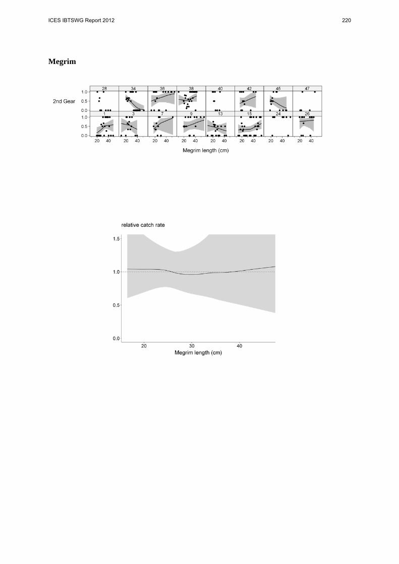
Megrim

ICES IBTSWG Report 2012 220

2 – Trip effect and combining haddock data from the two cruises. To eliminate a cruise effect and therefore enable the haddock data from the 2006 and 2009 cruises to be combined. This was achieved using the CD and DC hauls with the C gear as the control and the D gear as the test.

Because the haddock catches from the two cruises had different length distributions there was a possibility the analysis was being driven by the extremes of the combined distributions (between 16cm and 53cm). To eliminate this possibility a further analysis

ICES IBTSWG Report 2012 221

was performed using the overlapping distributions (between 28cm and 46cm). Again this was achieved using the CD and DC hauls with the C gear as the control and the D gear as the test.

ICES IBTSWG Report 2012 222

3 – Final analysis for each species from both cruises. In the absence of a ‘towing-order’ effect for all species and ‘trip-effect’ and ‘distribution-effect’ for haddock the CD and DC hauls were analysed using the C as the control and D as the test. Haddock

ICES IBTSWG Report 2012 223

Lemon sole

ICES IBTSWG Report 2012 224

Megrim

ICES IBTSWG Report 2012 225

Whiting

ICES IBTSWG Report 2012 226

GOV trawl geometry Comparisons from the Danish and Swedish NS-IBTS in Q3 2011 and Q1 2012 with RV Dana with reference to Scottish and German observations

ICES IBTS WG 2012

Lorient, 27-30 March

Kai Wieland

M. Jarnum

M. Jarnum

DTU Aqua

ICES IBTSWG Report 2012 227

DTU Aqua, Technical University of Denmark

Survey areas

-4° -2° 0° 2° 4° 6° 8° 10°

2

4 6

7

1

5

3

8

IBTS roundfish area

5 6 8 9 0 3 5 6 8 9 G0

29

30

31

32

33

34

35

36

37

38

39

40

41

42

43

44

45

46

47

48

49

50

51

52

1 station

2 stations (with >= 10 nm distance)

only if not coveredby other countries

GOV and CTD

CTD only

-4° -2° 0° 2° 4° 6° 8° 10°

5 6 8 9 0 3 5 6 8 9 G0

29

30

31

32

33

34

35

36

37

38

39

40

41

42

43

44

45

46

47

48

49

50

51

52

GOV and CTD

MIK

Survey area(as planned)

Cruise track

GOV invalid

no CTD

DEN 3Q 2011 DEN 1Q 2012

SWE

DEN: Survey areas differ between quarters

SWE: same survey area in Q1 and Q3,

only country in Skagerrak and Kattegat

DEN/SWE: Same vessel in 3Q 2011 and 1Q 2012 (RV Dana) but own trawl and doors, SWE gear lighter than DEN gear (Skipper’s impression and specifications in DATRAS)

ICES IBTSWG Report 2012 228

DTU Aqua, Technical University of Denmark

Warp length and depth

Kai Wieland Warp length (m)

150 250 350 450 550 650 750

Dep

th (m

)

0

50

100

150

200

250 DEN 3Q 2011 and 1Q 2012SWE 3Q 2011 and 1Q 2012SCO 3Q 2011 and 1Q 2012GFR 3Q 2011 and 1Q 2012Manual

ICES IBTSWG Report 2012 229

DTU Aqua, Technical University of Denmark

Warp length and Net opening

Warp length (m)

100 200 300 400 500 600 700

Net

ope

ning

(m)

2.5

3.0

3.5

4.0

4.5

5.0

5.5

6.0

6.5

7.0

7.5

DEN 3Q 2011 and 1Q 2012(60 m sweeps)DEN 1Q 2012 (110 m sweeps)SWE 3Q 2011 and 1Q 2012(60 m sweeps)SWE 1Q2012 (110 m sweeps) SCO 3Q 2011 and 1Q 2012(60 m sweeps)GFR 3Q 2011 and 1Q 2012(50 m sweeps)GFR 1Q 2012 (100 m sweeps)Manual

Net opening highly variable (at a given warp length) for all countries

None of the countries within the values given in the manual for the range of warp lengths

SWE: low net opening at short warp length

DEN: relative high net opening at short warp length

ICES IBTSWG Report 2012 230

DTU Aqua, Technical University of Denmark

Warp length and Door spread

Warp length (m)

100 200 300 400 500 600 700

Doo

r spr

ead

(m)

40

60

80

100

120

140

DEN (60 m sweeps)DEN (110 m sweeps)SWE (60 m sweeps)SWE (110 m sweeps) SCO (60 m sweeps)GFR (50 m sweeps) GFR (100 m sweeps)Manual

SCO does not change sweep length in Q1

SWE, DEN and GFR wider door spread than given in the manual at longer warp length when using the longer sweeps (Q1)

ICES IBTSWG Report 2012 231

DTU Aqua, Technical University of Denmark

Net opening / Door spread

Door spread (m)

40 60 80 100 120 140

Net

ope

ning

(m)

2.5

3.0

3.5

4.0

4.5

5.0

5.5

6.0

6.5

7.0

7.5 DEN (60 m sweeps)DEN (110 m sweeps)SWE (60 m sweeps)SWE (110 m sweeps) SCO (60 m sweeps)GFR (50 m sweeps)GFR (50 m sweeps) Relationship between

door spread and net opening:

- differ between countries

- differ between sweep length

ICES IBTSWG Report 2012 232

DTU Aqua, Technical University of Denmark

Door spread / Wing spread

Door spread (m)

40 60 80 100 120

Win

g sp

read

(m)

10

15

20

25

SCO (60 m sweeps)GFR (50 m sweeps)GFR (100 m sweeps)

DEN and SWE do not measure wing spread (no sensors available on Dana)

Relationship between door spread and wing spread differ considerably between sweep length and less between country

ICES IBTSWG Report 2012 233

DTU Aqua, Technical University of Denmark

Depth, Net opening and Door spread

Depth (m)

0 50 100 150 200 250

Net

ope

ning

(m)

2.5

3.0

3.5

4.0

4.5

5.0

5.5

6.0

6.5

7.0

7.5

Depth (m)

0 50 100 150 200 250

Doo

r spr

ead

(m)

40

60

80

100

120

140

DEN (60 m sweeps)DEN (110 m sweeps)SWE (60 m sweeps)SWE (110 m sweeps) SCO 3Q 2011 (60 m sweeps)GFR (50 m sweeps)GFR (100 m sweeps)Manual

for short sweeps:

DEN (and SCO) could use some longer warp length and shallower depths to bring net opening and door spread within in range given in the manual

SWE (and GFR) may try another kite

for long sweeps:

DEN, GFR and SWE may try shorter warp lengths (as long as bottom contact is ensured)

The considerable differences in the trawl geometry between the countries require adjustment

ICES IBTSWG Report 2012 234

DTU Aqua, Technical University of Denmark

Conclusions and recommendations for discussion No drastic changes because if ‘consistency’ must be maintained (in

particular in respect to the use of IBTS indices for stock assessments)

⇒ use long sweeps at depths > 70 m in Q1 continue / discontinue !?

Further adjustments in warp length (country specific) should be encouraged to meet the ranges of net opening and door spread given in the manual

The IBTS WG may investigate whether it is possible to provide indices (for demersal species) based on swept area estimates to accommodate the large difference of door spread at a given depth between countries Problems:

Interpolation of missing values (country and year specific, dependent on sweep length)

Relationship between door and wing spread not available for all countries and years

ICES IBTSWG Report 2012 235

P a g e | 1

1 ICES DATRAS FAQ For Data Submitters, version 1

ICES DATRAS FAQ FOR DATA SUBMITTERS ICES DATA CENTRE

Version 1, May 2012

ICES Headquarters, Copenhagen

ICES DATRAS FAQ FOR DATA SUBMITTERS

ICES DATA CENTRE

ICES IBTSWG Report 2012 236

P a g e | 2

2 ICES DATRAS FAQ For Data Submitters, version 1

FAQs for data submitters ................................................................................... 3

Getting started/General questions ................................................................................ 3

What is DATRAS Data Policy? .......................................................................................................... 3

How should my data files be formatted?........................................................................................ 3

Which units and codes should I use for the data I report? ............................................................. 3

How do I get access to DATRAS uploading page? ........................................................................... 3

How to submit my file to DATRAS? ................................................................................................. 3

I get a page error when trying to use DATRAS. What to do? .......................................................... 3

I’ve forgot my log-in details. What do I do?.................................................................................... 3

Who to contact?.............................................................................................................................. 3

Submission-related questions ....................................................................................... 4

What is the deadline for my submission? ....................................................................................... 4

What data quality control do my data pass through? .................................................................... 4

I cannot understand what the screening message means. What to do? ....................................... 4

I cannot screen or upload my file. I get a message “the survey selected does not include the country present in the file”. I report my country. What is wrong? ................................................ 4

I have uploaded my data file to DATRAS, but I cannot find my data on the download page ........ 4

Can I make a partial re-submission by haul or by record type? ..................................................... 5

What happens to the existing data when I re-submit my dataset? ............................................... 5

When I re-submit my data, is it possible to deliver the information about which corrections were made? .................................................................................................................................... 5

Specific issues ............................................................................................................... 6

How to report Data Type in HH-record, and how does it influence other fields? .......................... 6

What is CatIdentifier, and how do I use it for my data? ................................................................. 7

Which area/position should I report in my file? ............................................................................. 7

What should I report in the Ground rope weight field? ................................................................. 8

What is species validity (SpecVal)? ................................................................................................. 8

Species codes and species code types. .................................................................................... 8

I get an error message when I try to upload my data with TSN species codes. ............... 8

How do I convert my species codes from Aphia to TSN? ..................................................... 8

ICES IBTSWG Report 2012 237

P a g e | 3

3 ICES DATRAS FAQ For Data Submitters, version 1

FAQs for data submitters Getting started/General questions

What is DATRAS Data Policy? ICES operate an open access data policy adopted by the ICES Council in 2006. Aggregated data and raw data are freely available to download from the data products page on DATRAS.

To read more about ICES Data Policy, go to http://www.ices.dk/datacentre/datapolicy.asp. To read more about DATRAS adoption of data policy, visit http://datras.ices.dk/Home/Access.aspx#.

How should my data files be formatted? DATRAS accepts files formatted as CSV (comma separated values) documents, where records are separated by rows/lines, and fields are separated by commas (,) or semicolons (;).As a decimal separator points (.) should be used.

Structure of files should follow DATRAS reporting format. All fields should be present in the file. No blanks are accepted. In case no information is available for a field, -9 should be reported.

One file should contain all types of records (HH, HL, CA) per year, quarter, country, vessel, gear.

Which units and codes should I use for the data I report? In the DATRAS menu Reporting Format one can find descriptions of fields including data units and codes per survey.

How do I get access to DATRAS uploading page? If you are a new data submitter to DATRAS, write an e-mail to DATRAS data manager and Chair of the associated ICES Expert Group detailing your submitter status and requesting access to DATRAS.

How to submit my file to DATRAS? For most of the surveys direct upload by data submitters is now available. Please follow the instructions on the DATRAS uploading page. Please read the document “How to upload data into DATRAS” on the same page.

I get a page error when trying to use DATRAS. What to do? If you get an error page somewhere in DATRAS, this might mean that one or all of DATRAS web-services failed to function. Please contact DATRAS administration as soon as possible. Please attach the screenshot from DATRAS to your e-mail.

I’ve forgot my log-in details. What do I do? Your log-in information is the same as the one you use to access ICES sharepoint.

If you forgot your GroupNet password, go to http://www.ices.dk/groupnetpass/ to retrieve the new one.

Who to contact? If you have questions, please write to the DATRAS administration or call us on +45 3338 6700.

If your request requires input from experts or further discussion, post it on DUAP.

ICES IBTSWG Report 2012 238

P a g e | 4

4 ICES DATRAS FAQ For Data Submitters, version 1

Submission-related questions

What is the deadline for my submission? The list of deadlines for the current year can be viewed on DATRAS documents page.

What data quality control do my data pass through? Before a data file can be uploaded to DATRAS, it passes an extensive quality check provided by the screening utility called DATSU. The results of screening will be displayed on the DATRAS page and will be sent as a PDF report to your mailbox. The screening report can contain some errors and warnings about your data. Most of the errors are critical, and should be corrected. If the file contains critical error(s), further data uploading will be impossible until the errors are corrected. All warnings are non critical, so it is the decision of the data submitter whether to accept these warnings or make further data corrections.

In addition, DATRAS provides outlier graphs based on weight-length relation for species that have these variables reported in CA records. They allow the submitter to spot the outlying weight or length values right away.

I cannot understand what the screening message means. What to do? For more detailed information about the error/warning please press the question mark in the right column of the screening results table, see example below. If the help-page was not informative enough, contact DATRAS administrator for further assistance. Don’t forget to attach your file and screenshot of DATRAS page displaying the error message.

I cannot screen or upload my file. I get a message “the survey selected does not include the country present in the file”. I report my country. What is wrong? There could be several reasons for such a message.

Please check whether:

1. The country code used is as in http://www.ices.dk/datacentre/reco/reco.asp?sortby=Code&ref=4

2. If numbers have been formatted with a comma as the decimal-delimiter, change them to decimal points.

3. There may be a problem with your access rights to DATRAS. Contact DATRAS administrator. Include your file and screenshot of DATRAS page with error in your e-mail.

I have uploaded my data file to DATRAS, but I cannot find my data on the download page You may experience a delay from the time you submit the data until it can be found on the download page. This is because files uploaded to DATRAS are manually updated in the main data warehouse as part of the quality control process.

ICES IBTSWG Report 2012 239

P a g e | 5

5 ICES DATRAS FAQ For Data Submitters, version 1

To check whether the file was successfully uploaded, check your submission on DATRAS Submission Status page. If your submission with correct upload time is listed there, the upload was successful. If the submission is not on the list, try to upload your file once again, and then contact DATRAS administration.

Update of data on the web-page might take a few days. If the uploaded data need to be urgently available from DATRAS web-page for download, contact DATRAS administration for assistance.

Can I make a partial re-submission by haul or by record type? Currently, DATRAS does not facilitate partial re-submissions of any kind. The whole dataset per year, quarter, country, vessel, gear should be re-submitted.

What happens to the existing data when I re-submit my dataset? When a dataset is re-submitted and the DATRAS data warehouse is updated, the existing data are overwritten and are no longer available. We advise you to always keep a copy of previous submissions.

When I re-submit my data, is it possible to deliver the information about which corrections were made? At the last stage of uploading there is a box for remarks. In this box data submitters should specify what was changed in the re-submitted data. In the next DATRAS update it will be possible to view submitters’ remarks (if any) on the Submission Status page.

ICES IBTSWG Report 2012 240

P a g e | 6

6 ICES DATRAS FAQ For Data Submitters, version 1

Specific issues

How to report Data Type in HH-record, and how does it influence other fields? Data Type defines the use of data fields reported in HL-record. For information and examples on data type and related fields use please visit DUAP, Background and Working Documents section.

Data Type can be reported as R (raw data reported, sorted catch might be sub-sampled), S (bulk unsorted catch was sub-sampled), C (catch reported as CPUE).

Depending on the data type used, HL data fields will be reported as follows:

DataType R:

TotalNo – report the total number of fish of one species, sex, and category in the given haul;

CatIdentifier – report category within species and sex. The field can be used to categorize fish with different size or weight categories. Categories within one haul, species, sex, can have different sub-factors. The field cannot be reported as 0, use 1 if only one category is present.

NoMeas – report number of fish measured for the given haul or sub-sample, species, and sex.

SubFactor – sub-sampling factor by haul, species, sex, length. Value = or > 1. Make sure that TotalNo = NoMeas x SubFactor

SubWgt – report the total weight of sub-sampled fish reported in NoMeas.

CatCatchWgt – report catch weight of fish per species, sex, and category in the given haul (as in TotalNo).

HLNoAtLngt – report number of fish for this sex of this species, in this category in the haul. Make sure that TotalNo = Sum (HLNoAtLngt) x SubFactor or NoMeas = Sum (HLNoAtLngt).

DataType S:

TotalNo – report the total number of fish of one species, sex, and category in the given haul;

CatIdentifier – report category within species and sex. Categories within one haul, species, sex, can have different sub-factors. The field can not be reported as 0, use 1 if only one category is present.

NoMeas – report number of fish measured for the given haul or sub-sample, species, and sex.

SubFactor – sub-sampling factor by haul, species, sex, length. Value is always > 1. Make sure that TotalNo = NoMeas x SubFactor

SubWgt – report the total weight of sub-sampled fish reported in NoMeas.

CatCatchWgt – report catch weight of fish per species, sex, and category in the given haul (as in TotalNo).

HLNoAtLngt – report number of fish for this sex of this species, in this category in the haul. Make sure that TotalNo = Sum (HLNoAtLngt) or NoMeas = Sum (HLNoAtLngt)..

ICES IBTSWG Report 2012 241

P a g e | 7

7 ICES DATRAS FAQ For Data Submitters, version 1

DataType C:

TotalNo – report the total number of fish of one species and sex in the given haul, raised to 1 hour hauling;

CatIdentifier – report 1.

NoMeas – report number of fish measured for the given haul or sub-sample, species, and sex or report -9.

SubFactor – report 1.

SubWgt – report the total weight of sub-sampled fish reported in NoMeas or report -9.

CatCatchWgt – report the total catch weight per species per haul, raised to one hour of hauling.

HLNoAtLngt – report number of fish for this sex of this species in the haul adjusted to one hour of catching. Make sure that TotalNo = Sum (HLNoAtLngt).

What is CatIdentifier, and how do I use it for my data? The CatIdentifier is the ID number given to a particular subsampling for species, length and sex.

During the length distribution sampling, when a truly representative subsample cannot be selected, it is necessary to further sort the species into two or more size grades or categories.

That would usually mean that a group of larger (or smaller) fish is sorted away from the rest of the catch of the same species. In further processing, this category of fish would get a different sub-sampling factor than the rest of the catch of the same species in the haul.

Some examples about categorization can be read in the NS-IBTS survey manual (section “Length composition”)

The correct approach to report categorization to DATRAS is to use the field CatIdentifier. Then one size-group of species would get assigned CatIdentifier = 1, and will have a certain SubFactor reported, while the other size-group of the same species in the haul would get CatIdentifier = 2, and will have another SubFactor reported. There can be reported up to 5 categories per species in one haul.

If no categorizing was made, CatIdentifier should be reported as 1 as follows of that the whole catch was treated as one category.

Which area/position should I report in my file? There are several places in DATRAS, where area of fishing is reported.

Hauling coordinates and statistical rectangle are reported in HH-record. You can find more information about ICES statistical rectangles on http://geo.ices.dk/.

If sampling is made by areas that include depth strata, the strata are reported in the field “Stratum” in HH-record.

ICES IBTSWG Report 2012 242

P a g e | 8

8 ICES DATRAS FAQ For Data Submitters, version 1

In addition, in CA-records area types and area codes are reported according to the method of age sampling (with the prospect on how the survey indices are calculated). Look up http://www.ices.dk/datacentre/datsu/selrep.asp for stratum and area codes relevant for your survey.

What should I report in the Ground rope weight field? This issue is to be discussed during IBTSWG meeting 2012. For other surveys contact your expert group.

What is species validity (SpecVal)? Species validity is a code that allows DATRAS to sort which data should be used for indices calculation, and which should not. Species validity code is related to the haul validity code in HH-record. If the haul was invalid, or was used for calibration, all species caught in the haul will be not valid for data product calculation (that would be reflected in the SpecVal field). But the data might still be valuable for example. assessment of the age-length distribution of the species in the area or biodiversity studies.

Species codes and species code types. Please make sure that Species Code and Species Code Type follow the same type – For TSN codes, Species Code Type should be T; for Aphia/WoRMS species codes the Species Code Type should be W.

I get an error message when I try to upload my data with TSN species codes. For now, please overrule the error message and submit the data with TSN species codes. The error is there because DATRAS submissions were supposed to migrate to WoRMS species codes in the spring of 2012. However, not all countries are ready to submit in AphiaID, so for the time being all submissions must be made using TSN codes.

How do I convert my species codes from Aphia to TSN? Please have a look at the lookup table found on our species query tool page http://datras.ices.dk/Data_products/qryspec.aspx

ICES IBTSWG Report 2012 243

P a g e | 9

9 ICES DATRAS FAQ For Data Submitters, version 1

ICES DATRAS FAQ for Data Submitters

Version Number

Release Date

Note

1 May 8 2012 Initial version, reviewed by ICES Data Centre

ICES IBTSWG Report 2012 244

Working Document presented to the IBTSWG Lorient, 27-30th April 2012.

Comparisons between Megrim (IVa and VIa) CPUE indices derived from DATRAS exchange data and data received directly from national laboratories.

Norman Graham, Marine Institute, Galway, Ireland

Background

There has been no analytical assessment of megrim in ICES division VI since 2000 and no assessment of megrim in IV has ever been presented. Missing or low age sampling from both VI and IV has hampered the development of an age-disaggregated assessment approach. During WKFLAT (2011, 2012) and WGCSE 2011 work on an age-aggregated dynamic production model has been progressed for this stock and is currently undergoing review through an inter-benchmark process (IBP-MEG, 2012).

Input data for biomass dynamic model

Surplus production methods (Schaefer, 1954; Pella Tomlisson, 1969) offers a potential modelling approach to resolve the issue of data poor classification due to the absence of reliable catch at age data. Surplus production pools the overall positive contributory effects (growth and recruitment) with removals due to mortality into a single production function, thus the stock is considered solely in terms of biomass without regard for differences in age, size of sex structure. Surplus production models are commonly used when only relative biomass indices, either from survey or from commercial fisheries, and landings data are available.

Indices from 6 fishery independent surveys are used (Table 1). These comprise of the Scottish North Sea IBTS survey (IBTSWG, 2011), Scottish quarter 1 (ScoGFS-WIBTS-Q1) and quarter 4 (ScoGFS-WIBTS-Q4) West of Scotland survey and the Scottish (SAMISS-Q2) and Irish (IAMISS-Q2) dedicated anglerfish survey (Table 1) which provides estimates of absolute biomass and abundance (see Reid et al, 2007 for further details), however the survey also catches significant quantities of megrim, but as there are no estimates of catchability, for the purposes of this work, the indices are treated in a relative sense.

The uncertainty surrounding each survey index (observation error) can be estimated within the assessment model or estimated externally and entered into the assessment model as a fixed quantity. Bootstrapping provides estimates of uncertainty but these may be artificially small (unsuitable) to a fixed-station survey design. Stefánsson (1996) provides analytical methods for the estimation of the variance of the delta-gamma method but cautions against the use of those variance forms because of concerns regarding the correct number of degrees of freedom. Ultimately, the uncertainty of the delta-gamma method may best be estimated in a Bayesian framework. For the present analysis the mean delta-gamma CPUE estimates are used (for the IBTS surveys only) and allowed the model to estimate the measurement error of each survey.

ICES IBTSWG Report 2012 245

Number Survey Nationality Area Time Series 1 Sco-IBTS-Q3 Scotland IVa 1987 - 2011 2 Sco-IBTS-Q1 Scotland IVa 1987 - 2011 3 ScoGFS-WIBTS-Q1 Scotland VIa 1986-2011 4 ScoGFS-WIBTS-Q4 Scotland VIa 1986-2011 5 SAMISS-Q2 Scotland VIa*/IVa 2005-2011 6 IAMISS-Q2 Ireland VIa* 2005-2011

Table 1. Survey indices used for surplus production model. *VIa data from IAMISS-Q2 and SAMISS-Q2 combined into a single CPUE estimate with variance

Data Issues surrounding the IBTS survey indices

Initially, the CPUE indices from individual surveys were estimated from the exchange data extracted from DATRAS. Due to missing catch weight data per tow, catch weights were estimated by applying a standard mean weight at length to the numbers caught at length. A number of concerns were raised when comparing the total number of fish recorded and the sum of the length frequencies, used as a quality check before estimating the CPUE indices. As a consequence, it was decided to approach national laboratories to obtain the national survey data and to compare these with the exchange data obtained from DATRAS. Figure 1 shows the bootstrapped CPUE estimates for megrim derived from the DATRAS exchange data (left had panels) and contrasted with the bootstrapped CPUE estimates derived from the data received from national authorities. Unfortunately, only data from the UK (Scotland) was obtained, but it is clear that there are a number of discrepancies between the two, both in terms of CPUE trends and/or absolute estimates of CPUE (scale).

ICES IBTSWG Report 2012 246

Figure 1. Comparison of bootstrapped CPUE trends derived from DATRAS exchange data and bootstrapped CPUE derived from national (Scottish) data.

ICES IBTSWG Report 2012 247

It has not been possible at this stage to dig further into the possible causes of these differences, but an initial comparison of two positions from the two data sets suggests (particularly for IVa) that there are a substantial number of hauls given in national data set missing in the DATRAS exchange data (figure 2).

Figure 2. Two examples of missing observations when contrasting data received from national laboratories with those extracted from DATRAS exchange data.

Due to the apparent discrepancies shown in the example above, until such time as these are resolved, it was decided to only use the data obtained from the national laboratories as input into the biomass dynamic model. Obviously, this is a sub-optimal solution for obtaining and selecting input data for the assessment, ideally the data from all useful surveys should be used and that this should be housed and obtained from a central data base i.e. DATRAS

Conclusions

Further analysis and data quality checks may be required to ensure that data being uploaded to DATRAS is the same as data extracted using the DATRAS exchange query. In the case presented here, it is important to identify where and critically, why these discrepancies have occurred and if these are associated with the DATRAS then remedial steps e.g. further QA steps should be considered.

ICES IBTSWG Report 2012 248

Lorient, IBTS WG, 29 mars 2012

Thibaut Nebout(1), Aurélie Foveau (2), Sandrine Vaz(3), Nicolas Desroy (2)

(1) MNHN, CRESCO Dinard (2) Ifremer, CRESCO Dinard (3) Ifremer Boulogne-sur-mer

BenthicBenthic MacrofaunalMacrofaunal

Observations Observations OnboardOnboard

FishFish Assessment Assessment ResearchResearch

SurveysSurveys

ICES IBTSWG Report 2012 249

�� LackLack of information on offshore of information on offshore speciesspecies and and assemblages assemblages atat mesoscalesmesoscales

� The use of fish assessment research survey enablesthe observation of macrofauna on large geographicareas (trawl vs grab)

� Species collected by trawling represent essentially the sessile part of the macroinvertebrate fauna : the mostsusceptible to be disturbed by trawling activities

IntroductionIntroduction

ICES IBTSWG Report 2012 250

��Distribution of macroDistribution of macro--epibenthicepibenthic invertebratesinvertebrates usingusing

samplessamples collectedcollected duringduring bottombottom trawltrawl surveyssurveys

Distribution of Ophiotix fragilis (a

common brittle star)

Distribution of Liocarcinusholsatus (swimming crab)

Distribution of Aequipectenopercularis (Queen scallop)

ICES IBTSWG Report 2012 251

IBTS IBTS -- OSPAR OSPAR RegionRegion IIII

ICES IBTSWG Report 2012 252

� 1 species and 3 habitats threatened and/or declining

ICES IBTSWG Report 2012 253

AA-- Ocean Ocean quahogquahog -- ArcticaArctica islandicaislandica((LinnaeusLinnaeus, 1767), 1767)

ICES IBTSWG Report 2012 254

ArcticaArctica islandicaislandica

�A species in decline

� A sensitive species

� A threatened species

1972-1980 1990-1994

ICES IBTSWG Report 2012 255

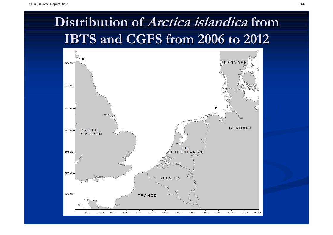
Distribution of Distribution of ArcticaArctica islandicaislandica fromfrom

IBTS and CGFS IBTS and CGFS fromfrom 2006 to 20122006 to 2012

ICES IBTSWG Report 2012 256

BB-- ModiolusModiolus modiolusmodiolus bedsbeds

ICES IBTSWG Report 2012 257

ModiolusModiolus modiolusmodiolus bedsbeds

�� LowLow resilienceresilience of the habitatof the habitat

�� HighHigh sensibilitysensibility to to physicalphysical disturbancedisturbance

ICES IBTSWG Report 2012 258

Distribution of Distribution of M. M. modiolusmodiolus bedsbeds fromfrom

IBTS and CGFS IBTS and CGFS fromfrom 2006 to 20122006 to 2012

ICES IBTSWG Report 2012 259

CC-- Sabellaria Sabellaria spinulosaspinulosa reefsreefs

ICES IBTSWG Report 2012 260

�An habitat in decline

Sabellaria Sabellaria spinulosaspinulosa reefsreefs

�A rare habitat

�A sensitive habitat

�A threatened habitat

�Ecologically significant

ICES IBTSWG Report 2012 261

Distribution of Distribution of Sabellaria Sabellaria spinulosaspinulosa reefsreefs

fromfrom IBTS and CGFS IBTS and CGFS fromfrom 2006 to 20122006 to 2012

ICES IBTSWG Report 2012 262

DD-- SeapenSeapen and and burrowingburrowing megafaunamegafauna

Virgularia mirabilis

Pennatula phosphorea

ICES IBTSWG Report 2012 263

PennatulaPennatula phosphoreaphosphorea

- No detailed mapping of this

habitat is available

- Limitations in knowledge

- The highest threat is thebottom trawling fisheries

ICES IBTSWG Report 2012 264

Distribution of Distribution of PennatulaPennatula phosphoreaphosphoreafromfrom IBTS IBTS andand CGFS CGFS fromfrom 2006 to 20122006 to 2012

ICES IBTSWG Report 2012 265

Distribution of Distribution of threatenedthreatened habitats habitats

plottedplotted againstagainst riskrisk

ICES IBTSWG Report 2012 266

ConclusionConclusion

�� This This kindkind of information of information maymay bebe veryvery relevant to relevant to plan plan

future future humanhuman activitiesactivities in the area and to in the area and to mitigatemitigate

potentialpotential bottombottom fishingfishing impactsimpacts

�� Use Use underwaterunderwater videovideo beforebefore eacheach bottombottom trawltrawl haulhaul to to

avoidavoid the destruction of the destruction of threatenedthreatened benthicbenthic habitatshabitats

�� Report Report ourour observations to the observations to the OSPAR habitat OSPAR habitat

mappingmapping programmeprogramme ((OSPARmapping@OSPARmapping@jnccjncc..govgov..ukuk ))

ICES IBTSWG Report 2012 267

ThankThank youyou for for youryour

attentionattention

ICES IBTSWG Report 2012 268

”Bad Hair Day” Acoustic Survey for Spawning Saithe in the North Sea 1st quarter

2012

Institute of Marine Research 14.02.2012

Introduction

Several attempts have been made to establish fishery independent survey series for saithe in the North Sea. Saithe is spawning in the first quarter and this is an attempt at an acoustic survey targeting spawning aggregations of saithe. It is likely that this is the time of year where the spawning stock is most accessible for a survey (forming spawning aggregations) and we believe that the area covered will be far less than during periods with more intense feeding and feeding migrations. Area covered

The choice of area coverage was based on logbook information from Norwegian fishermen for the period 2000 to 2011. On the average is well above 90% of the commercial catches taken within the survey area. Fishing further south along the Norwegian deep represents on average 1% of the total. 1st quarter biological samples from the commercial fishery within the survey area have generally a large mean weight indicating that most fishery is targeting spawning aggregations. Stratification

The survey area has been divided into 6 strata (see Figure 1). S3 and S4 are the strata with the highest proportion of catches followed by S2 and S6. The fishing effort itself is less and more concentrated in a more “narrow strip” and a shorter depth range than in S3 and S4. Strata S1 and S5 contains less fishing effort of a more sporadic nature varying between years. Traditional stratification assumes or utilizes more homogenous populations within the stratum and this may very well hold for population parameters. There is a strong tendency that estimates of fish abundance have a standard deviation proportional to the abundance. This

ICES IBTSWG Report 2012 269

implies that proportional sampling (density of samples) may be close to optimal in estimating total abundance (index/indices of abundance). Acoustic transects

Acoustic transects represents an integration over depth and distance and should and the result represents a reduction of the observed three dimensions to a single dimension (embedded in this is the assumption of no measurement error, which will not hold at shallow depths where objects directly in the path of the vessel can avoid detection). The acoustic observations may be biased due to a range of issues including species identification, “dead zone loss” and varying target strength (the average angle the acoustic signal “hits” the target/swimbladder with, may vary). See Figure 2 and Figure 3. Acoustic settings

See also Hansen, K. and Knudsen, H.P. 2006. The following should be viewed as guidelines: Bottom channel 10meters above bottom and use 0.5 meter bottom offset if conditions permits. At depths less than 200 meters the “bottom detection minimum” should be set within the range -40 to -45 dB. At larger depth or in poor weather conditions this threshold could be set as low as -55 dB. Integration of echo abundance is made using LSSS (Large Scale Survey System). SV threshold in LSSS should be -82 dB when storing acoustic records. Changing SV during scrutiny of echograms is a valuable tool for identifying some species groups. As an example will a threshold of -69 (±3dB) be quite effective to mask plankton echo. The acoustic values should be stored with 10 meter resolution vertically and 1 nm horizontally. Species groups

Group Target category Herring 1 Other pelagics 3 Cod 2 Haddock 2 Haddock 2 Saithe 1 Plankton 3 Trawl stations

Trawl station information is used twice. Firstly to assist in distributing echo abundance between species groups. Secondly as to further characterize and convert echo abundance into numbers of fish. This in combination with trawl samples not being part of a formal survey

ICES IBTSWG Report 2012 270

design can lead to the introduction of serious bias. On the other hand can relatively large proportions occupy a relatively small area and trawl samples from such areas will be very valuable to characterize the structure of the fish population while this is independent to the overall abundance based on the formal acoustic survey transects. The number of trawl stations should be higher in areas/strata with the most fish and one should aim for at least 5 trawl station in the strata S2, S3, S4 and S6. Catch rates of saithe are highly variable and one must consider using manual weighting of each station using “good judgement” while considering the acoustic observations. Trawl information can be re-used meaning that trawl stations taken outside a stratum can also be included. For this survey this may be the solution for stratum S1 and S5. Length distributions

Estimates of length distributions are essential for converting echo abundance into numbers of fish. This information is also used in distributing echo abundance between species so there is a need for length samples of all fish “visible” in the water column. Please note that any prediction of sA distribution between species based on trawl samples should adjust for length dependent selectivity of the sampling trawl. Smaller fish (like Norway pout) is caught with less efficiency than larger fish and this should be taken in to account and properly adjusted for. Biological sampling

Indices of abundance (numbers at length) is further characterized based on biological samples (weight, age, sex, maturity stage, spawning checks etc.) and are sampled with a further stratification on length (5 specimen per 5cm length groups of saithe). This implies that any generation of age length keys can’t use unweigthed information. As a rule of thumb should each single fish observation be given a weighting factor. Weighting factors should add to the corresponding abundance index (by stratum and lengthgroup). Environmental data

Distributional changes over time (between years) will be an issue and additional information is needed when searching for causal mechanisms. Information from CTD stations is one such source of information. See Figure 4. References

Hansen, K. og Knudsen, H.P. 2005. Prosedyre for innsamling og bearbeiding av akustikkdata versjon 3.0. Håndbok for innsamling og bearbeiding av akustikkdata. Havforskningsinstituttets kvalitetssystem. Hansen, K. og Knudsen, H.P. 2006. Instruks for innsamling og bearbeiding av akustikkdata versjon 2.0. Håndbok for innsamling og bearbeiding av akustikkdata. Havforskningsinstituttets kvalitetssystem.

ICES IBTSWG Report 2012 271

Hansen, K., Knudsen, H.P. og Ona, E. 2006. Instruks for tolking og kvalitetsmerking av akustikkdata versjon 2.0. Håndbok for innsamling og bearbeiding av akustikkdata. Havforskningsinstituttets kvalitetssystem. Mjanger, H., Hestenes, K., Svendsen, B. V. og Wenneck, T. d. L. 2007. Håndbok for prøvetaking av fisk og krepsdyr. Versjon 3.16, opplag januar 2011. Havforskningsinstituttets kvalitetssystem. Wenneck, T. d. L., Hestenes, K., Svendsen, B. V. og Else, H. 2010. Prosedyre for håndtering av fisk og krepsdyrdata versjon 2.4.7. Havforskningsinstituttets kvalitetssystem. Tables

Design Stratum Description Area Distance Length of Direction Comments(nm2) between course

transects tracks(nm) (nm)

S1 Schiehallion 636.1 12 315°/135°S2 Otter bank 1125.9 6 327 315°/135°

ver. 1 S3 Tampen W 1508.2 6 327 315°/135°(6/12 nm) S4 Tampen N 2039 6 225°/45°

S5 Tampen S 2694.8 12 732 225°/45°S6 Tampen E 1176.3 6 248 225°/45°

1634

S1 Schiehallion 636.1 14 315°/135°S2 Otter bank 1125.9 7 314 315°/135°

ver. 2 S3 Tampen W 1508.2 7 694 315°/135°(7/14 nm) S4 Tampen N 2039 7 198 315°/135°,225°/45°

S5 Tampen S 2694.8 14 315°/135°S6 Tampen E 1176.3 7 211 225°/45°

1417

ICES IBTSWG Report 2012 272

Figures

Figure 1 Strata system. Schiehallion, Otter bank, Tampen

Figure 2 Course tracks: Alternative 1 with parallel transects 6/12nm spacing

ICES IBTSWG Report 2012 273

Figure 3 Course tracks: Alternative 2 with parallel transects 7/14nm spacing

Figure 4 Suggested CTD station for the design with 7/14 nm distance between acoustic transects. Appendix I

Detailed course tracks version 1 (6/12 nm distance between transects) Strata 1 & 2:

Point no Dist Cum dist Lat Lon

ICES IBTSWG Report 2012 274

W 000 0 0 59°59.5161 N 003°14.0186 W W 001 31.7 31.7 60°21.8619 N 003°59.1724 W W 002 12.3 43.9 60°31.4539 N 003°43.6816 W W 003 20.1 64.1 60°17.1843 N 003°14.8975 W W 004 6.2 70.3 60°11.9498 N 003°21.5991 W W 005 11.7 82 60°03.6876 N 003°05.0098 W W 006 6.2 88.2 60°08.5615 N 002°57.2095 W W 007 11.8 100.1 60°16.8577 N 003°14.2383 W W 008 7 107.1 60°23.5995 N 003°10.3931 W W 009 14.1 121.1 60°13.6415 N 002°50.2881 W W 010 6.4 127.6 60°19.1981 N 002°43.8062 W W 011 29.4 157 60°39.9764 N 003°26.1035 W W 012 11.3 168.3 60°37.3372 N 003°03.6914 W W 013 17.9 186.2 60°24.7392 N 002°37.8735 W W 014 6.4 192.6 60°30.5347 N 002°32.1606 W W 015 19.9 212.5 60°44.5724 N 003°00.8350 W W 016 6.1 218.6 60°49.1852 N 002°52.6227 W W 017 17.6 236.2 60°36.6770 N 002°27.2168 W W 018 6.3 242.5 60°41.8328 N 002°19.8010 W W 019 16.4 258.9 60°53.3854 N 002°43.5864 W W 020 6.2 265.1 60°57.0430 N 002°33.3142 W W 021 15.9 281 60°45.7809 N 002°10.2429 W W 022 6.2 287.3 60°49.1852 N 001°59.5313 W W 023 16.4 303.7 61°00.8001 N 002°23.4814 W W 024 6.2 309.9 61°04.8421 N 002°13.8135 W W 025 17.2 327.1 60°52.6904 N 001°48.7646 W

Strata 3: Point no Dist Cum dist Lat Lon W 000 0 0 60°56.7495 N 001°39.4812 W W 001 17 17 61°08.8226 N 002°04.3103 W W 002 6.2 23.2 61°12.9268 N 001°54.6423 W W 003 15.2 38.4 61°02.1570 N 001°32.4500 W W 004 6.2 44.6 61°06.1699 N 001°22.7271 W W 005 16.1 60.8 61°17.5762 N 001°46.4575 W W 006 6.3 67.1 61°22.8984 N 001°39.4812 W W 007 17.4 84.5 61°10.6241 N 001°13.7732 W W 008 6.4 90.8 61°15.0948 N 001°04.3799 W W 009 18.7 109.6 61°28.2058 N 001°32.2852 W W 010 6.5 116 61°33.6551 N 001°25.0342 W W 011 17.9 133.9 61°20.8981 N 000°58.6670 W W 012 6.5 140.4 61°26.7359 N 000°52.8442 W W 013 17.1 157.5 61°38.8273 N 001°18.1128 W W 014 6.1 163.6 61°43.9598 N 001°10.9717 W W 015 18.1 181.7 61°31.0106 N 000°44.4946 W W 016 6.7 188.3 61°33.4715 N 000°31.5308 W

ICES IBTSWG Report 2012 275

W 017 21.3 209.7 61°48.8435 N 001°02.7319 W W 018 5.9 215.6 61°52.1097 N 000°52.2949 W W 019 25.7 241.2 61°33.5240 N 000°14.9414 W W 020 7.1 248.3 61°34.9362 N 000°00.3296 W W 021 27.7 276.1 61°54.9051 N 000°40.9790 W W 022 6.5 282.6 61°57.3344 N 000°28.1250 W W 023 19.2 301.8 61°43.3869 N 000°00.1099 W W 024 8.5 310.3 61°51.9028 N 000°00.2197 E W 025 10.9 321.2 61°59.8121 N 000°15.7104 W W 026 6.2 327.4 62°02.1833 N 000°03.5156 W

Strata 4 & 5:

Point no Dist Cum dist Lat Lon W 000 0 0 62°02.9566 N 000°00.8789 E W 001 8.3 8.3 61°54.6985 N 000°00.4395 E W 002 13.4 21.7 62°04.6037 N 000°19.7754 E W 003 7.4 29.1 62°04.3975 N 000°35.5957 E W 004 24.1 53.2 61°46.8195 N 000°00.4395 E W 005 8.8 62 61°38.0712 N 000°00.0000 E W 006 35.7 97.7 62°04.3975 N 000°50.9766 E W 007 7 104.6 62°02.1325 N 001°05.0391 E W 008 88.5 193.1 61°00.1080 N 001°07.2363 W W 009 19.2 212.3 60°59.8953 N 000°27.6855 W W 010 42.7 255 61°30.5397 N 000°34.2773 E W 011 6.7 261.7 61°32.2163 N 000°20.6543 E W 012 37.6 299.4 61°59.2450 N 001°16.0254 E W 013 6.1 305.5 61°54.9055 N 001°25.2539 E W 014 33.9 339.4 61°30.7495 N 000°35.1562 E W 015 6.5 345.8 61°29.2816 N 000°48.3398 E W 016 28.3 374.1 61°49.1038 N 001°30.9668 E W 017 6.2 380.4 61°43.6996 N 001°37.5586 E W 018 61.3 441.7 61°00.3211 N 000°07.0313 E W 019 15.8 457.5 60°59.8953 N 000°39.5508 E W 020 38.6 496.1 61°26.7625 N 001°37.1191 E W 021 7.9 504 61°28.0227 N 001°20.8594 E W 022 15.1 519.1 61°38.6974 N 001°43.2715 E W 023 6.2 525.3 61°34.1002 N 001°52.0605 E W 024 10.4 535.7 61°26.9727 N 001°36.2402 E W 025 5.9 541.6 61°22.1357 N 001°43.2715 E W 026 12.5 554 61°30.7495 N 002°02.1680 E W 027 6.1 560.2 61°26.9727 N 002°12.2754 E W 028 37.8 598 61°00.3211 N 001°16.4648 E W 029 16.4 614.4 61°00.3211 N 001°50.3027 E W 030 10.4 624.8 61°07.7624 N 002°05.2442 E W 031 5.9 630.6 61°12.2130 N 001°57.3340 E W 032 15.1 645.7 61°22.7672 N 002°19.7461 E

ICES IBTSWG Report 2012 276

W 033 6.7 652.4 61°16.8643 N 002°26.3379 E W 034 12.6 665 61°08.1866 N 002°07.4414 E W 035 5.6 670.6 61°03.3012 N 002°13.1543 E W 036 13.1 683.7 61°12.2130 N 002°32.9297 E W 037 6 689.7 61°07.7624 N 002°41.2793 E W 038 15 704.7 60°57.3368 N 002°18.8672 E W 039 7.4 712.1 60°50.0692 N 002°21.9434 E W 040 19.8 731.9 61°04.3643 N 002°50.0684 E

Strata 6:

Point no Dist Cum dist Lat Lon W 000 0 0 61°00.1084 N 002°58.8574 E W 001 22.8 22.8 60°44.1704 N 002°25.4590 E W 002 6.5 29.2 60°37.9306 N 002°28.9746 E W 003 24.9 54.1 60°55.3086 N 003°05.4492 E W 004 6.4 60.5 60°49.5332 N 003°11.1621 E W 005 23 83.5 60°33.3993 N 002°37.7637 E W 006 5.8 89.3 60°29.0742 N 002°45.6738 E W 007 20.6 109.9 60°43.5258 N 003°15.5566 E W 008 6.1 116 60°38.1462 N 003°21.2695 E W 009 19.4 135.4 60°24.3056 N 002°53.5840 E W 010 6.1 141.5 60°18.6543 N 002°58.4180 E W 011 17.6 159.2 60°31.0220 N 003°23.9063 E W 012 7.8 167 60°23.2200 N 003°24.7852 E W 013 17.6 184.6 60°10.8031 N 002°59.7363 E W 014 7.9 192.4 60°02.9204 N 002°59.2969 E W 015 20.1 212.5 60°17.1302 N 003°27.8613 E W 016 7.2 219.7 60°10.1474 N 003°31.3770 E W 017 14.3 234 60°00.0661 N 003°11.1621 E W 018 8.1 242.1 59°59.8464 N 003°27.4219 E W 019 6.1 248.2 60°04.2363 N 003°35.7715 E

Appendix II

Detailed course tracks version 2 (7/14 nm distance between transects) Strata 1 & 2:

Point no Dist Cum dist Lat Lon W 000 0 0 59°59.4190 N 003°14.4580 W W 001 31.1 31.1 60°21.0595 N 003°59.2822 W W 002 14.7 45.8 60°32.6551 N 003°40.8252 W W 003 18.9 64.8 60°19.2108 N 003°13.7988 W W 004 7.6 72.3 60°12.5629 N 003°21.0498 W W 005 11.9 84.2 60°04.1388 N 003°04.1309 W W 006 7.4 91.6 60°10.0503 N 002°55.1221 W W 007 13 104.7 60°19.2108 N 003°13.7988 W

ICES IBTSWG Report 2012 277

W 008 8.2 112.9 60°27.0284 N 003°08.5254 W W 009 14.9 127.8 60°16.5979 N 002°46.9922 W W 010 7.4 135.2 60°23.0151 N 002°39.7412 W W 011 27.6 162.8 60°42.3553 N 003°19.7314 W W 012 9 171.8 60°43.5376 N 003°01.4942 W W 013 19.7 191.5 60°29.7356 N 002°32.7100 W W 014 8.2 199.7 60°37.4036 N 002°26.9971 W W 015 17.2 216.8 60°49.3311 N 002°52.2656 W W 016 7 223.9 60°54.2522 N 002°41.9385 W W 017 16.4 240.2 60°42.7856 N 002°17.9883 W W 018 7.5 247.8 60°47.2948 N 002°05.6836 W W 019 16.3 264 60°58.5216 N 002°29.8535 W W 020 7.4 271.4 61°03.3127 N 002°18.2080 W W 021 17.2 288.6 60°51.1511 N 001°53.1592 W W 022 7.5 296.1 60°55.7476 N 001°41.0742 W W 023 17.5 313.5 61°08.0919 N 002°06.5625 W Strata 3, 4 & 5 (parts of S4):

Point no Dist Cum dist Lat Lon W 000 0 0 61°12.9650 N 001°56.0156 W W 001 18.6 18.6 60°59.9067 N 001°28.5498 W W 002 21 39.6 60°59.9067 N 000°45.2637 W W 003 17.3 57 61°12.0126 N 001°10.9717 W W 004 7.4 64.4 61°06.7125 N 001°21.7383 W W 005 16.5 80.8 61°18.2478 N 001°46.1279 W W 006 7.7 88.5 61°24.5671 N 001°37.1191 W W 007 17.8 106.2 61°12.0126 N 001°10.9717 W W 008 7.5 113.8 61°18.0368 N 001°01.5234 W W 009 18.2 132 61°30.5512 N 001°29.2090 W W 010 7.7 139.7 61°37.1430 N 001°20.8594 W W 011 53.2 192.9 61°00.0133 N 000°01.5381 W W 012 20.7 213.6 60°59.9067 N 000°41.0889 E W 013 47.8 261.3 61°33.6932 N 000°29.2236 W W 014 8.1 269.5 61°30.9704 N 000°45.2637 W W 015 17.6 287 61°43.2947 N 001°11.6309 W W 016 7.4 294.4 61°49.2189 N 001°02.4023 W W 017 21.8 316.2 61°33.9022 N 000°29.6631 W W 018 10.8 327 61°33.5883 N 000°07.0313 W W 019 28.2 355.2 61°53.2613 N 000°49.6582 W W 020 8.1 363.2 61°56.3644 N 000°33.8379 W W 021 80.3 443.5 60°59.9067 N 001°25.6934 E W 022 21.3 464.8 61°00.1198 N 002°09.6387 E W 023 88.5 553.3 62°02.3489 N 000°02.1973 W W 024 8.4 561.7 61°59.3609 N 000°18.8965 W W 025 43.3 605 61°29.1861 N 000°46.8018 E W 026 14.9 620 61°39.9605 N 001°08.5547 E

ICES IBTSWG Report 2012 278

W 027 34.8 654.8 62°04.3061 N 000°15.8203 E W 028 10.9 665.7 62°04.5119 N 000°39.1113 E W 029 27.9 693.5 61°44.7516 N 001°20.8594 E

Strata 4 (remaining part):

Point no Dist Cum dist Lat Lon W 000 0 0 61°46.7273 N 001°34.7022 E W 001 25.7 25.7 61°28.6640 N 000°56.2500 E W 002 9.4 35.1 61°27.8247 N 001°15.8057 E W 003 17.1 52.2 61°39.9609 N 001°41.0742 E W 004 7 59.1 61°34.6350 N 001°50.5225 E W 005 10.9 70 61°27.0895 N 001°34.0430 E W 006 7 77 61°21.9898 N 001°43.9307 E W 007 11.7 88.7 61°30.2373 N 002°01.2891 E W 008 6.9 95.6 61°25.9867 N 002°12.6050 E W 009 14.8 110.4 61°15.5029 N 001°50.7422 E W 010 6.9 117.3 61°10.2655 N 002°00.0806 E W 011 14.6 131.9 61°20.6206 N 002°21.5039 E W 012 7.1 139 61°14.5518 N 002°29.0845 E W 013 13.6 152.6 61°04.9609 N 002°09.0894 E W 014 6.9 159.4 60°59.9071 N 002°18.6475 E W 015 13.1 172.5 61°09.1000 N 002°37.8735 E W 016 6.9 179.4 61°04.5884 N 002°48.6401 E W 017 18.5 197.9 60°51.5798 N 002°21.5039 E

Strata 6:

Point no Dist Cum dist Lat Lon W 000 0 0 60°43.8069 N 002°25.4590 E W 001 23 23 60°59.9608 N 002°59.0771 E W 002 6.9 29.9 60°53.9325 N 003°06.1084 E W 003 24 53.9 60°37.0270 N 002°31.2817 E W 004 6.8 60.7 60°31.7912 N 002°40.0708 E W 005 22.1 82.8 60°47.2952 N 003°12.1509 E W 006 7.2 89.9 60°40.7968 N 003°18.3032 E W 007 20 109.9 60°26.6497 N 002°49.6289 E W 008 7 116.9 60°20.8968 N 002°57.6489 E W 009 18.2 135.1 60°33.7903 N 003°23.7964 E W 010 9.4 144.5 60°24.3724 N 003°24.2359 E W 011 17.4 161.9 60°12.1813 N 002°59.2969 E W 012 9.4 171.3 60°02.8233 N 002°59.8462 E W 013 19.7 190.9 60°16.5983 N 003°28.0811 E W 014 7.8 198.8 60°09.0123 N 003°31.9263 E W 015 12.6 211.4 60°00.0788 N 003°14.1284 E

ICES IBTSWG Report 2012 279