i'S' Report flapINFO 0020-1

.Atomic EnergyControl Board

Commission de controlede 1'energie atomique

DEVELOPMENT AND COMPARISON OFTECHNIQUES FOR ESTIMATING DESIGNBASIS FLOOD FLOWS FOR NUCLEAR

POWER PLANTS - PHASE I

INFO-0020-1

11III

DEVELOPMENT AND COMPARISON OF

(TECHNIQUES FOR ESTIMATING DESIGNBASIS FLOOD FLOWS FOR NUCLEAR

POWER PLANTS - PHASE I

IIIIIiIIIII{ May 1980

A Report prepared for theAtomic Energy Control Board

S.I. Solomon & Associates Ltd.

IIII "The Atomic Energy Control Board Is not responsible

for the accuracy of the statements made or opinions

I expressed in this publication and neither the Board

nor the author(s) assume(s) liability with respect

• to any damage or loss incurred as a result of the

use made of the information contained in this

publication."

IIIIIIIIIIIII

A B S T R A C T

Estimation of the design basis flood for Nuclear Power Plants

can be carried out using either deterministic or stochastic techniques.

Stochastic techniques, while widely used for the solution of a variety of

hydrological and other problems, have not been used to date (1980) in

connection with the estimation of design basis flood for NPP siting. This

study compares the two techniques against one specific river site (Gait on

the Grand River, Ontario). The study concludes that both techniques lead

to comparable results, but that stochastic techniques have the advantage of

extracting maximum information from available data and presenting the results

(flood flow) as a continuous function of probability together with estimation

of confidence limits.

s i s u t i i

Une estimation d'une inondation d« reference pour Centralea

Nucleaires a ate faita an employant soit das aathodaf deterministiques

ou stochastiques. Lea methodes stochastiques, quoique employees largement

pour la solution d'une variete de probleae* hydrologiques ou autres, n'ont

pas eta employees jusqu'ici (1980) an regard d1estimation d•inondations de

reference pour la choix das sites pour Centrales Nucleaires. Dana cette

etude, las deux techniques sont comparees pour la location d'une riviere

bian spacifiqua (Grand River 1 Gait, Ontario). II en ast conclu qua las

deux techniques dormant das resultata sensibleaent pareila, mais qua lea

methodes stochastiques ont l'avantage d'axtraire la maximum d1information

des donnees diaponibleo at da presenter las resultats (debit d'inondation)

come une fonction continue da probability ainni qu'una estimation des limites

de confianc*.

S. I. SOLOMON&

ASSOCIATES LIMITED

HYDROLOGY

WATER RESOURCES

REMOTE SENSING

203 DAWSON STREET

WATERLOO, ONTARIO

N2L !S3 Tel. (519)885-2717

DEVELOPMENT AND COMPARISON OF TECHNIQUES FOR ESTIMATING

DESIGN BASIS FLOOD FLOWS FOR NUCLEAR POWER PLANTS

A Report Prepared for

ATOMIC ENERGY CONTROL BOARD OF CANADA

May 1980

DEVELOPMENT AND COMPARISON OF TECHNIQUES FOR

ESTIMATING DESIGN BASE FLOOD FLOWS FOR NUCLEAR POWER PLANTS

TABLE OF CONTENTS

LIST OF TABLES

LIST OF FIGURES

1. SUMMARY, CONCLUSIONS AND RECOMMENDATIONS

1.1 Summary

1.2 Conclusions

1.3 Recommendations

2. ' INTRODUCTION

2.1 Background

2.2 Purpose

2.3 Scope

2.A Basic data

2.5 Description of study basin

3. APPROACH

3.1 PMP-PMF estimation

3.2 Time series analysis and synthesis

4. PMF ESTIMATION

4.1 PMP estimation

4.2 PMF using "Official Unit Hydrograph"

4.3 PMF using "Updated Unit Hydrograph"

4.4 PMF using calibrated rainfall-runoff model

4.5 Discussion on PMP-PMF values and uncertainties

5. EFFECT OF DAMS AND RESERVOIRS

5.1 Brief Description of Dams and Reservoirs

5.2 Actual and Potential Effects on Flood Peaks

5.3 Effects on Statistical Characteristics of Flood Peaks

5.4 Erroneous (or Malevolent) Operation

5.5 Dam Failure

6. TIME SERIES ANAYSIS AND SYNTHESIS

6.1 Time ser ies analysis

6.2 Time series synthesis

6.3 Discussion on maximum flows of various probabi l i t ies

7. COMPARISON OF MAXIMUM FLOWS BY VARIOUS TECHNIQUES

7.1 Comparison of peak flows by various techniques

7.2 Credibility of estimated PMF's and of flows of low probability.

8. TECHNIQUES FOR LEVEL AND VELOCITY DETERMINATION

8.1 Level estimation

8.2 Velocity determination

9. EXTENSION OF METHODOLOGY TO ESTIMATION OF DESIGN BASISVALUES FOR LOW FLOWS AND WAVES

9.1 Deterministic approach to low flows

9.2 Time series approach to low flows

9.3 Deterministic approach to waves

9.4 Time series approach to waves

APPENDICES

Al. AES Letter

A2. Non-linear Distributed Model

A3. Code for Time Series Analyssis and Synthesis

A4. Code for Generation of Normally Distributed Random Numbers

A5. Letter from H. G. Acres to Secretary Treasurer of Grand RiverConservation Commission

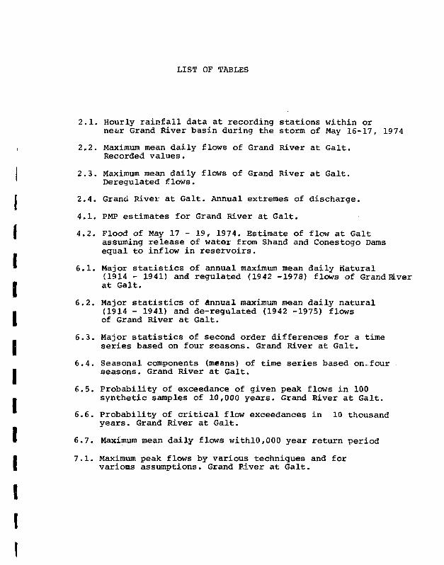
LIST OF TABLES

2.1. Hourly rainfall data at recording stations within ornear Grand River basin during the storm of May 16-17, 1974

i 2,2. Maximum mean daily flows of Grand River at Gait.Recorded values.

j 2.3. Maximum mean daily flows of Grand River at Gait.

Deregulated flows.

I 2.4. Grand River at Gait. Annual extremes of discharge.

4.1. PMP estimates for Grand River at Gait.I 4.2. Flood of May 17 - 19, 1974. Estimate of flow at Gait

assuming release of water from Shand and Conestogo Damsequal to inflow in reservoirs.

* 6.1. Major statistics of annual maximum mean daily Satural(1914 - 1941) and regulated (1942 -1978) flows of Grand RLver

I at Gait.

6.2. Major statistics of Annual maximum mean daily natural

1 (1914 - 1941) and de-regulated (1942 -1975) flowsof Grand River at Gait.

6.3. Major statistics of second order differences for a timeI series based on four seasons. Grand River at Gait.

6.4. Seasonal components (means) of time series based on..fourI seasons. Grand River at Gait.

6.5. Probability of exceedance of given peak flows in 100. synthetic samples of 10,000 years. Grand River at Gait.

6.6. Probability of critical flow exceedances in 10 thousandyears. Grand River at Gait.

6.7. Maximum mean daily flows withl0,000 year return period

1 7.1. Maximum peak flows by various techniques and forvarions assumptions. Grand River at Gait.

III

LIST OF FIGURES

2.0. Limits of the Study Basin, Grand River at Gait.

2.1. PMP estimates according to Bruce (1956).

2.2. PMP estimates according to Soil Consevation Service (1975).

2.3. Flows of Grand River at Gait during the 16 - 19 my, 1974 Flood.

2.4. Estimation of isohyets of storm of May 16 - 17, 197 4.

2.5. Radar imagery on May 17, 1974.

2.6. Typical hydrograph at Gait*

2.7. Example of data contained in the grid square system fordistributed model of Grand River.

4.1. The "Official 6 hour unit hydrograph.

4.2. Hydrograph resulting from application of a thunderstorm PMP +to "Official" unit hydrograph.

4.3. Hydrograph separation for derivation of "Updated 6 hourUnit Hydrograph".

4.4. "Updated" 6 hour Unit Hydrograph.

4.5. Hydrograph of PMF resulting from application of a thunderstam PMP+ JjPMP to "UPdated" Unit Hydrograph.

4.6. Grand River at Gait: Calibration of non-linear distributed model.

4.7. Grand River at Gait: Validation of non-linear distributed model.

4.8. Probable Maximum Flood based on distributed non-linear model.

5.1. Shand Dam - Project arrangement.

5.2. Conestogo Dam - Project arrangement.

5.3. Peak flow versus recurrence interval, Grand River at Gait,1914 - 1941,.

5.4. Peak flow versus recurrence interval, Grand River at Gait,1942 - 1957.

List of Figure, page 2

5.5. Peak flow versus recurrence interval, Grand River at Gait,1958 - 1975.

5.6. Comparison between inflow and outflow, Shand Dam, Flood of17 - 18 May, 1974.

6.1. Correlogram for selection of time series interval.

6.2. Grand River at Gait: Synthesized curve of probability ofexceedance of maximum mean daily flows.

6.3. Relationship between mean daily and instantaneous maximum fiws.Grand River at Gait.

8.1 Stage - discharge relationship for Mississipi River,Tarbert Landing, La. (1/23/69 - 3/26/69).

8.2. Stage - discharge relationship for Mississipi River,Tarbert Landing, La. (2/9/66 - 4/11/66).

8.3. Comparison between recorded and calculated water profilesat Gait for the 1974 peak flood flow.

8.4.Level variation in time during a flood event.

8.5. Schematic representation of stage - discharge relationshipduring a flood event.

8.6. Water profile along a river reach-during a flood event.

...I

1. STJMMARY, CONCLUSIONS AND RECOMMENDATIONS

This study was carried out at the request of AECB on the

basis of contract 23SQ. 87055-8-0266 issued by DSS. In spite of its

budget and time limitations ($10,750 and 10.5 months) the study is

comprehensive and provides the requested information on all problems

included in the "statement of work" of the contract. This was made

possible due to the excellent co-operation of A2CB, in particular Messrs.

R.J. Atchison, K. Asmis and F. Campbell, and of Grand River Conservation

Authority through Ms. L. Mirshall. The latter has kindly supplied SIS &

A with the basic data required for the time series analysis.

1.1 Summary

Design basis floods have been calculated for Grand River at

Gait using basically the methodology recommended by IAEA (SG S10A). This

consists of two different approaches. The first, which is considered as

the basic one, requires determining the Probable Maximum Precipitation

and its use in a rainfall-runoff model for estimating the corresponding

Probable Maximum Flood (PMF). The second consists of estimation of the

value of the design basis flood flow as the flow with a very low return

probability (of the order of 10 to 10 years) determined through

techniques of time series analysis and synthesis.

The PMP-PMF technique was applied using values of PMP obtained

from two different studies and two different rainfall—runoff models to

illustrate the uncertainty that is involved in -the application of the

technique. Thus the application of the PMP value as determined in one

study and the "official unit hydrograph" leads to a PMF value of about

400,000 cfs, whereas the application of a PMP value determined in another

1.2

study and a distributed non-linear rainfall-runoff model leads to a PMFThe

value of about 2,400.000 cfs./*'ost credible value of PMF appears tc be that

resulting from the application of the lower value of PMP to the distributed

non-linear rainfall-runoff model resulting in an estimated PMF of 1,460,000

cfs.

The application of the time series technique leads to the conclusion

that daily mean maximum flows with a return probability of 10 years has

an estimated value of approximately 1,400,000 cfs. Taking into account that at

very high flows the ratio between maximum instantaneous and daily mean

maximum flows /about 2, one may conclude that flows with return probability

of 10 years are practically of same magnitude as the PMF.

The two existing major dams in the study basin would fail in the

case of PMP occurring in the basin. In the case of concomitant arrival

at the study site of the two resulting flood waves, the resulting discharge

would be of about 3,000,000 cfs.

1.2 Conclusions

The comparison of the two techniques indicates that they lead

basically to comparable results. The uncertainty related to the application

of the PMP-PMF technique appears to be larger tha'i that resulting from

time series analysis and synthesis. However, this conclusion should be

tempered by the consideration that in this particular case a time series

having a length of over 60 years was available, a situation rarely en-

countered at most potential NPP sites. On the other hand, due to budget

and other limitations, the available fund of meteorological data has not

been fully utilized in the study. A significant portion of this uncertainty

relates to the use in one case of a linear unit hydrograph model based on

a flood which is not representative of maximized flood generating conditions.

1.3

The methodology recommended by IAEA (SG-S10A) is basically

sound, but its application requires in-depth investigations on PMP

and development of non-linear rainfall-runoff models calibrated on

the basis of hydrological data measured at the site or in similar basins

and including exceptional hydrometeorological events. The conventional

application of the unit hydrograph technique may lead to non-conservative

results.

There are significant similarities between the statistical

properties of low flows and wave characteristics on one hand and

maximum flows on the other. This indicates that the time-series

analysis-synthesis technique could be essentially applied in a similar

manner to the estimation of design basis values of low flows and waves.

1.3 Re commendations

The techniques applied in this pilot study should be further tested

in connection to real-life case studies. Simulation of a decision making

process at the design stage should be carried out using the data available

at the point in time when these decisions were mads. These dtcisions

should be compared with those that would be taken if all currently

available data were used. Conclusions on the significance of data and

cost of correcting design decisions should be attempted. Situations

requiring regional as well as local (site specific) hydrological data

should be considered.

A critical review of PMP estimates in various areas of interest

in Canada should be made. The results of this review should be used

to define and reduce the uncertainty related to PMP estimates.

PMF estimates should be preferably obtained using a non-linear

rainfall-runoff model. If a unit hydrograph technique is used it

1.4 I1

should be based on a flood which was generated by conditions that are I

as close .is possible to those maximizing runoff volume and particularly

flood peak. Corrections for non-linearity and changes in river basin |

conditions should be considered. _

The time series analysis and systhesis technique tested in

this pilot study should be experimentally applied to the determination I

of other design basis values such &s wave levels, low flows (and

levels). Such application should be facilitated by the generation I

of a large fund o: normally distributed random numbers (with mean zero

and standard deviaiton of one). Tine series of data should be used '

only after careful detection and elimination of non-homogeneities I

related to man's activity. Comparisons with deterministic techniques

should also be made to assess their results from a probabilistic view- I

point.

2.1

2. INTRODUCTION

2.1 Background

The safety as well as the operation reliability of

nuclear power plants (NPP's) requires a detailed analysis of the

hydrological characteristics of the area of the NPP's site and of the

related river basins. One major characteristic of particular sig-i

nificance to the safety of the NFF is the design basis flood.

I Estimation of the design basis flood for NPP's can be

carried out using either deterministic or stochastic techniques.

• This is recognized by the international hydrologic community and is

| reflected in the current draft of the IAEA Safety Guide on this

subject (IAEA, 1979).

I Deterministic techniques have been used in a number of countries

for estimation of t>; design basis flood for NPP sites. Stochastic

I techniques, while widely used for the solution of a variety of

I hydrological and other problems, have not been used to date (1980)

in connection with the estimation of design basis flood for NPP siting.

j Therefore AGCB has initiated a study aimed at comparing the two techniques

when used to estimate the design basis flood at a given site. Whereas

the study site and related basin are not considered for locating a

NPP, they are characteristic from the veiwpoint of hydrologic problems

to be expected at a typical inland NPP site.

The deterministic technique is based on three major steps.

The first involves the estimation of the Probable Maximum Precipitation

(PMP). The second requires the development of a suitable rainfall-runoff

model. And the third the estimation of the Probable Maximum Flood by

inputting in the rainfall-runoff model the value of the PMP.

The stochastic technique involves two phases. The first •

represents the analysis of the time series of flow records available I

at the site. In the course of this analysis the flow data are decomposed

.into two sets of components. The first set can be considered to have I

a deterministic nature and includes astronomic (seasonal) effects,

jstorage effects, and the effects of changes in conditions in the •

river basin reflected in jumps and trends. The second set of components I

is considered to include only random (probabilistic) effects, some of

which are local in nature, some regional. The latter may appear to be I

at the source of exceptional events recorded during the measurement

period. The second step comprises the estimation of floods of various •

probabilities of exceedance by synthesis of the random components and 1

recombination with the deterministic ones. Due recognition is given

in the stochastic technique as recommended in the IAEA guide to the I

sampling errors inherent both in the deterministic and random components.

The proper allowance for these errors in the synthesis phase enables I

generation of samples having statistics different from but compatible l

with those of the recorded sample and the estimation of confidence

limits of the results obtained.

The two techniques, when applied with reasonable adequate

data, can be expected to provide reasonably close results since both

represent the combination of maximization processes on observed data.

This requires however that the Maximum Probable Flood (PMF) is compared

to a flow of very small probability of exceedance which can be considered

to be about 10 - 10~ p.a.

While the deterministic technique is already widely used

for the design of NPPs, -here are some obvious advantages in the use

2.3

of the stochastic technique:

it enables the use of all the information available;

- it permits estimation of confidence limits;

it provides a basis for developing similar consistent

techniques for estimating other design basis values;

- it is more objective than the deterministic technique.

The major drawback of the stochastic technique is the

fact that while it has been successfully tested for relatively

large probabilities of exceedance it has not yet been compared with

results obtained from PMP values that is for extremely small probabilities

of exceedance of the order of 10 - 10 p.a.

2.2 Purpose

The purpose of the proposed study is to provide the

methodology for the application of the stochastic technique

of estimating design basis flood flows for NPPs and develop on

the basis of an example a comparison between the deterministic

and stochastic techniques. This comparison has the following

objectives:

- to check the consistency of the results;

to assess which technique is more suitable for various

site characteristics and conditions of data availability;

- to provide a basis for the development of similar techniques

for estimation of design basis values of other phenomena

such as low flows and levels, waves, winds

II

2.3 Scope

This study is considered to be exploratory in nature and :•

therefore its scope is limited to methodology development and

demonstration of feasibility on the basis of one example. Consequently, I

the scope of the proposed study includes the development at one m

river gauging station (Gait on the Grand River, Ont.) of the

following: I

- estimation of the PMF by deterministic techniques;

I- estimation of the relationship between the flood flow

and the corresponding probability of exea<»dance up to

a value of 10 - 10 p.a. 1- estimation of effects of changes in the river basin I

land-use and land-cover and reservoir construction

on the design basis flood calculations. |

- estimation of the effects on the results of faulty ,g

dam operation. *

In addition methodological discussions is provided on the I

following:

- estimation of flood levels from flood flow data and |

topographic - hydraulic surveys; .

- application of the techniques to ungauged sites; '

- possibilities of extending the stochastic technique

to the estimation of design basis values for low

flow and levels, wind, and waves.

The Grand River at Gait was selected because it has a

realtively lond period of record, has problems of non-monogeneity '

of the time series due to man's activity and was convenient to use

2 . 5

as an example because several studies including rainfall-runoff

model studies have been carried out earlier for this basin. The l imi ts of

tne Grand River bas in a re shown i n F igu ie 2 . 0 .

2.4 Basic data

The following data were required for the study:

- PHP time-space variation;

- Precipitation and flow data on major storms in

the river basin;

- The "official unit hydrograph";

- Physiographic datt' for the distributed rainfall

runoff (non-linear) model;

- Time series of recorded maximum daily flows of

each month corrected for change in storage in

man-made reservoirs for the period of record;

- Time series of instantaneous annual maximum flows

2.4.1 PMP time-space variation

In the earlier stages of the Project it was envisaged

that Atmospheric Environment Service of the Environment and Fisheries

Department will carry out a parallel study to the one herein reported

on the estimation of PMP in Southern Ontario. However, this was not

possible (see Appendix 1) and, at the advice of AES, an earlier

study by Bruce (1957) was used for this purpose. The pertinent

figure from this paper which has been used as the best available

estimate of PMP time-space distribution in Southern Ontario is

reproduced in this report as Figure 2.1.

2.6

As a check of these data, the PMP estimates for Eastern

United States* adopted Soil Conservation Service (197 5) have been

used and the pertinent figures are reproduced in this Report as

Figure 2.2.

2.4.2 Precipitation and flow data on major storms

These were obtained partly from the Grand River Conservation

Authority and partly form AES. As will be shown furthe^ the May 1974

storm and corresponding flood can be considered as the most extreme

recorded flood event and have been retained for the calibration of

various models used in the study. The basic data regarding the

precipitation and river flow during this event are shown in figures

2.3 and 2.4 and Table 2.1. Radar imagery for Southern Ontario during

the May 1974 storm was also obtained from AES. Samples of this imagery

are shown in Figure 2.5.

2.4.3 The "official" unit hydrograpb

This has been obtained from a document prepared on behalf

of Grand River Conservation Authority by Phillips Engineering and

reproduced in this Report as Figure 2.6. As can be readily observed

from the document„ the unit hydrograph used has a triangular shape.

The peak flow of this unit hydrograph is approximately 24,000 cfs.

*The PMP isohyets are extrapolated over Southern Ontario.

2.7

2.4.4 Physiographic data for the distributed (non-linear)rainfall-runoff model

These were obtained in digitized form from an earlier

study carried out by the Ontario Ministry of Environment with

assistance from Shully I. Solomon & Associates. The initial

2data bank used in the Ministry s study was based on a 2 x 2 Km

square grid system. In later modelling studies Shully I. Solomon

& Associates have concluded that this level of detail was excessive

and the data were recalculated for the purpose of this study using

2a 6 x 6 Km grid. Examples of the digitized physiographic data in

this grid system required for the rainfall-runoff model are shown in

Figure 2.7. More details on these data are provided in Appendix 2.

2.4.5 Time series of recorded regulated maximum daily flows foreach month

This data was obtained in computer compatible tape from

the Grand River Conservation Authority (GRCA). They were checked

against similar data obtained from the Inland Waters Branch of

Environment Canada. These data are shown in Table 2.2.

2.4.6 Time series of maximum daily flows for each month,corrected for changes in storage

These data were also obtained from GRCA. Thus time

series has been provided by GRCA only for the period 1941-1975. As

this period covers all events of interest to this study the omission

of the data in the last four years did not affect in any significant

way the results of the study. These data are shown in Table 2.3.

2.8 I

2.4.7 Time series of recorded instantaneous annual maximum flows

These data have been obtained from the Inland Waters Branch

of Environment Canada (Table 2.4). They reflect the effects of I

operation of the three reservoirs in the river basin, i.e., they are

not corracted for changes in storage. This correction cannot be

calculated because of lack of the required data.

IIIIIIIIIIIII

3.1

3. APPROACH

The main purpose of this study is to estimate the Probable

Maximum Flood (PMF) using deterministic techniques for a given river and

location, estimate maximum flows of very low recurrence probability

(10 - 10 per year) for same river and location using stochastic

techniques and compare the results. This comparison should provide

indications on the relative acceptability and conservatism of the two

techniques.

The estimation of the PMF requires first the estimation of

the Probable Maximum Precipitation (PMP). The latter was considered

to be extraneous input to this study and therefore the methodology for

its estimation is not described in this study.

Section 3.1 describes the approach to PMF estimation i.e. the

deterministic techniques. Section 3.2 describes the approach to estimation

of maximum flow of very low recurrence probability using a stochastic

technique. Both approaches are basically those described in IAEA (1979),

expanded however to the level of detail required for practical applications.

3.1 Deterministic methods

Deterministic methods are those methods for which most of the

parameters and their values may be explained by physical relationships and

are mathematically definable. When deterministic methods are used to

determine the PMF, a PMP analysis is carried out and the resulting

hyetograph is used as input into a deterministic rainfall-runoff model which

produces the PMF as an output. Although the rainfall-runoff model is

conceptually deterministic, any "deterministic" model has in fact a

built-in statistical character because its ;srameters are estimated through

a calibration process, and PMP itself is affected by important uncertainties.

3.2

PMP can be estimated on the basis of a detailed and comprehensive

analysis of the most severe storms on the meteorological record for the

region of interest coupled with the analysis of other meteorological

factors, (Paulhus, 1973). According to the US practice a rainfall event

used to estimate PMF consists of two storms: the PMP and 1/2 PMP. The smaller

storm is assumed to precede or to follow the PMP, with the most critical

time sequence being used. If the PMP is caused by convective activity

(thunderstorms) the interval between the beginning of the two storms can

be assumed to be 24 hours in most areas of the world.

A widely used rainfall-runoff model for computing PMF is the

unit hydrograph (World Meteorological Organization, 1969a; Linsley et al, 1975)

This model was used as one of the two considered in this study and is

further discussed in 3.1.1. Because of underlying assumptions of linearity

and of uniformity of precipitaton excess over the river basin and other

simplifying assumptions, unit hydrographs derived from small floods may

not express the proper flood characteristics of the basin when applied

to large storms (Amorocho, et al, 1971). Therefore it is required

that unit hydrographs used in PMF estimation should be based on floods

representing excess precipitation of about one third or more of the PMP.

However in most cases it is preferable to use other rainfall-runoff models

which are not based on assumptions of linearity.

The application of the hydrograph technique is also limited to

2

relatively small basins (of the order of a few thousand km ). For larger

basins the application of the technique is debatable.

A number of other rainfall-runoff models may be used to transform

PMP into PMF. Some of these models are described in HMO (1975). Any of

these models when selected for PMF estimation has to be validated by split

sampling techniques.

3.3

In basins in which land—use land-cover conditions have changed

recently or are expected to change over the lifetime of the NPP, it is

necessary to use models that take such changes into consideration (Gupta

and Solomon, 1976). This model was used as the second one tested in this

study and is further discussed in 3.1.2.

3.1.2 The unit hydrograph model

The unit hydrograph model enables ready estimation of flow

resulting from a given net precipitation if several assumptions are

accepted.

The unit hydrograph technique was originally developed by

Sherman (1942). Although many refinements and adjustments to regional

conditions have been suggested by a number of investigations, the basic

principles as presented by Sherman remain the same. A detailed presentation

of the unit hydrograph technique at the practical application level has

been made by the US Bureau of Reclamation (1965). This has been used

extensively in this section.

3.1.2.1 Definition

The unit hydrograph, or unitgraph, is a device used to estimate

streamflow resulting from a given excess (net) precipitation. It is defined

as the hydrograph of storm runoff at a given point that will result from an

isolated event of rainfall excess occurring within a unit of time and spread

in an average pattern over the contributing drainage area. Rainfall excess

is that portion of the rainfall that enters the stream channel as storm

runoff. A "unit of time" is an interval that is brief enough so that

fluctuations of the intensity of rainfall during the interval will not

materially affect the shape of the resulting hydrograph. Its duration

3.4

will depend generally upon the size of the drainage area and may range from

one hour or less for small watersheds to 24 hours for very lari;t> watersheds.

In general, unit duration should not exceed about one-fourth or, at the most

one-third of the concentration time of the basin. In the actual prediction

of storm flow the terms "unit hydrograph" and "unitgraph" are used in a

more restricted sense, to designate the unitgraph that represents exactly

one inch of runoff from the contributing area.

i-

3.1.2.2 Basic assumptions

The derivation and application of the unit hydrograph are based

on the following assumptions:

i) The effects of all physical characteristics of a given drainage basin,

including shape, slope, surface detention, permeability, drainage pattern,

and channel sotrage, are reflected in the shape of the storm runoff hdyrograph

for that basin.

ii) At a given point on a stream, the discharge ordinates of different storm

hydrographs generated by rainfall occurences of same duration are mutually

proportional. Therefore, if thp ordinates of each storm hvdrograph are divided

by the volume of excess rain that produced it, the resulting unitgraphs will

be identical in shape.

ii?) The hydrograph of storm discharge that would result from a series of

bursts of excess rain or from continuous excess rain of variable intensity

may be constructed from a series of overlapping unitgraphs, each resulting

from a single increment of excess rein of unit duration, each having their

ordinates multiplied by the corresponding precipitation excess.

3.5

3.1.2.3 Effect of storm characteristics

The perfect unitgraph, representing runoff generated at a rate

that represents the average areal pattern in every part of the basin and

remains constant throughout the duration of the burst, is never found in

practice. A unitgraph derived from observed data will invariably reflect

some of the characteristics of the storm that produced it. The efore,

in judging its applicability to a particular storm, the following considera-

tions must be kept in mind:

i) Higher momentary intensities of rainfall produce a higher peak

and a steeper unitgraph for the same volume of runoff. In general, rains

showing large hourly amounts may be assumed to have high momentary intensities.

Such rains also produce greater depths in all contributing channels, improving

their hydraulic conditions and shortening the time of concentration. This in-

creases the tendency toward a high peak and a steep unitgraph.

ii) A unitgraph results from a unit excess rain occurring within a

"unit" of time. If the time unit (or observed duration) is too long,

random variations in the rainfall rate will have so great an effect upon

the shape of the unitgraph that it cannot be applied to other storms. The

shorter the unit duration the better the results are likely to be.

iii) Unitgraphs from excess rain of longer duration are broader and

less steep than those from shorter rains. An unadjusted unitgraph is

strictly applicable only to excess rainfall increments of the same duration

as that from which it was derived.

iv) Excess rain that is intermittent within the unit of duration, or has

a high intensity near the beginning or end of the unit, not in normal proportion

to the average intensity, may produce an abnormally shaped unitgraph. The

amount of distortion is much less when the ratio of the duration to the lag-

3.6

I Iuu- is small. hag-time is defined as the time interval between tlio ccntroiil

of the precipitation graph and the peak of tlie liydrograpli.

v) The areal distribution of excess rain over the basin affects the

shape of the unigraph. If the heaviest rain is near the headwaters, the

accession limb will be less steep and the peak lower than if the storm

is centered lower in the basin. Ordinarily, storms well centered in the

basin, with reasonably heavy precipitation extending to all of the boundaries,

are considered the most suitable for the derivation of unitgraphs. In some

cases, however, it is desirable to assume a design storm centered low in

the basin in order to produce a more critical peak, and the unitgraph

should be derived from storms similarly located.

vi) Rainbursts moving down the basin tend to produce higher peaks

than stationary bursts. Those moving up or across the basin tend to

produce lower peaks. Bursts moving across a fan-shaped drainage pattern may

also produce secondary peaks.

vii) River basin characteristics that influence the shape of a unit

hydrograph may change in time. It is not acceptable to use a unit hdyrograph

derived from a storm that occurred before such changes took place to estimate

flows for the basin with changed conditions.

3.1.3 Derivation of unit hydrograph

There are several techniques used for the derivation of the unit

hydrograph. Although a number of processes are common to all methods, the

more conventional approach is the one outlined in the following steps:

i) Plotting of the discharge hydrographs for the gaging station

and determination of the behavior of ground-water flow.

3.7

ii) Subtraction of ground-water discharge and plotting of Uydrogr;ipliH

of storm discharge.

iii) Determination of periods of rainfall excess.

iv) Isolation and comparison of unitgraphs.

The general procedure of unit hydrograph estimation consists of

the following steps:

i) The compound event of discharge to be analyzed is selected and

the ground-water and residual flows are estimated and subtracted.

The unit duration of excess rainfall to be used is selected. The storm

discharges in cfs at unit intervals are picked off and tabulated.

The values are denoted as:

Qx > Q2 ' •'• Q i " " Q n

ii) The total amount of excess precipitation pertinent to the

compound event, and the increments of precipitation for the individual

unit time periods are estimated as accurately as possible. The sum of

the excess precipitation increments must equal the total runoff. The

excess precipitation in interval i is denoted as p..

iii) The runoff, in inches, of the compound event for the first

interval is computed as P-ih, = Q, where h, is the ordinate of the unit

hydrograph for the selected unit duration, h, is determined from this relation.

The computation is continued for second time interval from equation p^h, + P2hi =

which is used to determine h,. For the third interval h 3 is determined from the

relation p-h.+Pjl^ + Pj^^ = Q3 etc-

iv) The resulting hydrograph is examined for shape and corrections are made

if shape is not satisfactory. Slight changes in assumed groundwater and residual

flow are usually sufficient to produce satisfactory results.

3.8 iII3.1.4 Nonlinear distributed model

This technique was developed by Solomon & Associates (1972)

with Hit' purpose of developing a rainfall-runoff model which ror.onnizos I

the non- linear character of the rainfall-runoff relationship and the

non-uniformity of precipitation distribution and basin characteristics. I

In addition this model makes it possible to investigate the effects of •

changes in land-use laad-cover on the hydrological characteristics of

a river basin, in particular its maximum flows. •

The model has been described in detail by Gupta and Solomoi.' (1976)

and Solomon and Gupta (1976). These papers and the computer code of the M

model algorithm are given in Appendix 2. Only the algorithm for a m

snow - free basin is considered in this report as all applications of "

the model were for such situation. A description of a snowmelt subroutine •

that can be interfaced with the model to be applied during periods when the

basin has a snow cover can be found in Solomon & Associates (1976). The |

model has been applied to six river basins in Southern Ontario and a _

river basin in British Columbia. The model has been successfully used ™

in 1976 by Ontario Ministry of the Environment to simulate flood events I

in the Grand River basin.

I3.2 Stochastic Method

Stochastic methods are techniques of combined deterministic *

and statistical analysis and synthesis of time (space) series of data B

IIwith the purpose of extending such series and defining from the extended

series the magnitude of rare events. To put stocahstic methods in proper I

relation to the deterministic ones, one may state that the former attempt

to determine by the analysis-synthesis process the asymptote of the I

frequency curve that is directly estimated by the latter. The application I

3.9

of stochastic methods in hydrology has been discussed by Kisiel (1969),

Yevjevich (1972, 1976), Karvelishvili (1967), Kotegoda (1975) etc.

Because of the combined deterministic—statistical treatment of

the time series of data, it is possible to estimate the error or the

confidence limits affecting the results obtained from a stocahstic method.

This provides a basis for estimating the risk related to the use of certain

design basis values.

Stochastic methods can be applied to determine flood peaks or

flood levels of various return periods. Since for many applications in NPP

siting the most important hydrologic parameter is the extreme water level

rather than the extreme flow, the direct analysis of time series of water

levels may eliminate the difficult computation steps required for estimating

the levels corresponding to the selected design flow. However, in contrast

to the deterministic methods, the stochastic methods do not provide a con-

tinuous flood hydrograph and related information on rate of change in flow

(levels). Therefore, when stochastic methods are applied it is necessary

to make additional hydrologic computations to estimate a reasonably conser-

vative set of hydrologic parameters required for NPP siting and design.

Such parameters include at least: discharge peak and variation during the

flood event; and velocities, average and variation in the cross section

for important discharge values including the peak one. As these hydrological

characteristics are easier to obtain when deterministic methods of flood

estimation are used, it appears advisable to apply both techniques and use

the stochastic technique to evaluate the probability of the deterministically

estimated peak flood. This was in fact the approach used in this study.

3.10

i.2.1 Stoc.-ili.stic Analysis

III

Stochastic methods of analysis of time (space) series starts

from the assumption that such a series represents a numerical expression I

of a process generated by a limited number of definable and significant

causes, and an infinite number of small causes. The first type of •

causes* ar«? i/.'Mally identified in the analysis and their effect removed •

from the data series. The residual component, which presumably represents

the effects of a large number of small causes is then subject to statistical I

analysis. As a result of this analysis, one obtains a series of parameters

of the time (space) series that define the significant causes and the I

statistical characteristics of the residual component. If the hypothesis •

is valid that the residual component represents indeed the result of a

large number of small causes, then the corrollary is that its distribution I

is normal and can be defined by two parameters (mean and standard deviation).

Tests of normality of the residual distribution can be thus used to indicate I

if the hypothesis is acceptable or not. In case of significant departure •

of residuals from normality the analysis must be iterated and the search

for important factors leading to non-normality of the residuals expanded. I

It should be pointed out that the parameters defining the significant causes

as well as the residual distribution are only estimates of the actual values ||

since they are defined on the basis of a limited number of data (a sample) M

belonging to an infinite population. Thus, the parameters are affected by

errors and this must be recognized in the stochastic synthesis. I]

i IIn fact in some actual cases of time series analysis it may happen that 'the effect of a significant cause is identified, but the cause itself isnot. t

3.11

3.2.2 Stocahstic Synthesis

Having determined the time (space) series parameters, it is in

theory possible to express the flood of a given probability of exceedance

in terms of these parameters. However, in practice the statistical mathe-

matics are intractable (Natural Environmental Research Council, 1975).

Therefore a long sequence of flows is generated by a Monte Carlo technique

and the probability of the extreme estimated from it.

In order to account for the errors of the time series parameters,

the synthesis by Monte Carlo techniques should extend not only to the

synthetic generation of the random component, but also to the generation

of a number of various samples of the parameters which have normal or

occasionally other distributions* and standard deviations equal to the

corresponding standard error of estimation.

The model must be validated by dividing the input-output data

available into two or more samples using some of the samples to calibrate

the model, and the input of the other samples to synthesize outputs which

are compared to the observed ones; the errors thus computed are compared

to errors of the calibration set, and statistical or judgemental inferences

made about the validity of the model. The judgemental inferences should be

supported by facts which may explain the change in the time series parameters

from one sample to another. This is termed the "split sampling" technique.

The parameters finally used, however, shall be based on the use of the entire

set of data.

3.2.3 Application of Stochastic Methods

Although stocahstic methods require the availability of computer

technology, the application of stochastic methods should be made by means

of techniques that can be readily understood and checked at each step in

This is the case of the auto-correlation coefficient.

3-12 .[

Ithe course of the computation. A number of techniques for analysis and

synthesis of time series have been developed (Hufschmidt et al, 1966; I

Florinn <•! ill, 1971; Kottegoila, 1970; Yiwji; v Icli, 1972, 1976). Anv »l

those or other techniques is acceptable, provided that It demonslrah]y shows •

that the residuals arrived at have a distribution that is not statistically . I

different from a normal one and that the synthesis process takes into account

the error of estimate of the time series parameters. In addition the practical I

limitations of some techniques as outlined by Askew, et al (1971) should be

considered when selecting a synthesis technique. I

The stochastic technique can be applied both to gauged and ungauged . I

sites. Only the technique for gauged sites is discussed here because only

this technique has been used in the study. For ungauged sites see Solomon I

and Jolly (1976).

A site is considered gauged in the following circumstances: I

(a) If there is a long period of record at the site. A long period .

of record is defined for middle and higher latitudes (north of

40° N and south of 40° S) as 30 years and for lower latitudes I

as 50 years of record, provided there have been no extreme

meteorological events* in the region that have not affected the |

relevant basin; otherwise 50 and 70 years respectively. The extension _

to a period of 50 resepctively 70 years of record is required because

if the basin has not been subject during such period of record to a I

storm that is of an exceptional intensity compared to the usual storms

experienced by it, one could safely assume that the basin is for a J

reason or another (topographic, topographic location, etc.) sheltered

from such storms. Evidence that this assumption is correct should be

obtained through detailed meteorological analysis.

Such extreme meteorological events are those that appear on usual probabilitycurves as outliers and may have been recorded either by the meteorologicalnetwork or by the hydrological one or both.

3.13

(b) If the period of record can be extended by correlation with one or

two other gauges to a period of record equivalent to that indicated

above. The computation of the equivalent number of years should be

carried out as indicated by Fiering (1963). Actual extension is carried

out using complete correlation equations, including synthesis of the

random component, so that there is no reduction in variance of the

extended time series.

(c) If it can be demonstrated that the period of record provides a time

series of data having an error variance less than the error variance

obtained from a regional analysis. This check should be made in accordance

with the methodology developed by Matalas et al (1968). In the latter

case it must also be shown that there have been no extreme meteorological

events in the region that have not affected the relevant basin. Otherwise

allowance must be made for such events.

The time series to be used consists of the series of maximum

instantaneous or maximum daily flows* within a selected time interval At,

The latter is selected by considering various successively longer time intervals

selecting the corresponding maximum flows, eliminating the seasonal component

as shown below and computing the autocorrelation coefficients for the various

intervals. The time interval selected should be the last but one for which the

autocorrelation coefficient becomes insignificant.on flows

Since the effect pi various causes is multiplicative rather thanof flows

additive, time series/^re analyzed after a logarithmic transformation of

the data.

The use of instantaneous raaximums would be preferred if data are availablein this form. However, in most cases maximum daily flows will be consideredand relationships between maximum dailies and instantaneous maximums used tocorrect the final results.

3.14

The time series with the selected time interval is then

analyzed for ilefinnblo significant oaures Mini tlioir effect eliminated.

The usual definable slgni I'leant causes tlxat should bi1 eonsUlered art':

(a) seasonal variation ce meteorological conditions

(b) causes that may produce trends (e.g. urbanization, deforestation)

(c) causes that may produce jumps (construction of large reservoirs,

diversions)

(d) effect of storage

The seasonal effect is removed from the time series by subtracting

from each value the mean value corresponding to the given season. Obviously,

where At is one year or longer the seasonal effect does not exist. Thus for

each value Q... where i represents the year and j the season the value:

is calculated where Q.. is the logarithm of the flow for the given i

season, j year, and (X is the mean for the i season.

Trends can be detected by graphical and statistical analysis

(Yevjevich, 1972) of the time series and search of causes. Graphical analysis

can be carried out by means of moving - average graphs. Detected trends

are removed only if statistically significant at the 95% confidence level

and supported by evidence of physical activity in the basin, or significant

at the 99% level*. Trends are considered in the computation by their linear

approximation. Where a trend in the mean has been detected for a period

starting from A. and ending at A which are m At apart, and at the last

Note that trends of increasing (decreasing) levels may occur due to aggradation(degredation) without necessarily corresponding to increasing trends in flows.

3. i5

point A represents a total departure from the average up to A of 6.,S L K_L -L

each value A In the interval is corrected as follows

where b is the number of time intervals separating A.. from A, ,.ii kl

Jumps (steps) are also identified by graphical and statistical

analysis (Yevjevich, 1972) and their existence accepted using conditions

equivalent to those set up for trends**. If a positive jump 6, occurs in

the mean starting from value A mn the value 62 is added to all

values A.. preceding A mn

The effect of storage is removed by computing the autocorrelation

coefficient r for the series A., corrected for trends and jumps as shown

above. The removal of the effect is made by computing e.. values from

relationship:

e.. time series represents the random component of the time

series.

**Attention has to be paid to temporary jumps that may occasionally occurparticularly in connection with the filling of large reservoirs.

3.16 I

IThe standard deviation S, the coefficient of skew C .and the _

I

- changes with time of the storage characteristics of the basin

leading to trends and/or jumps in the value of S.

The standard error (E ) of each of the time series parameters

llnll

Icoefficient of kurtosis k of e . are computed. Tests to show that C

and k are not significantly different from zero and 3, respectively

(tests of normality of the distribution of e .) are carried out

(Yevjevich, 1972). If outliers are found to be the cause of non- ormality, I

they are considered as one additional special significant cause (e.g.,

hurricanes in areas with infrequent occurrences of hurricanes, i~e jams •

of exceptional size, etc.) and treated as such, i.e., removed and introduced •

at random intervals equivalent to intervals of their observed occurrence.

The statistical characteristics of outliers are synthesized on the basis of the I

observed statistics by Monte Carlo techniques as shewn further for other parameters

of the time series. m

If after consideration and removal of outliers e.. is not normally •

distributed the analysis is iterated. In iteration the following additional

possible causes of non-normality are investigated: •

- seasonal variation in storage leading to a seasonal variable r

1I

P", (i.e. Q. , r, S) is computed using the formulas shown in Yevjevich I

(1972) and N sets of values of each parameter are obtained by means of

appropriate Monte Carlo techniques. The number N is obtained by dividing I

the number of years for which synthesis is intended by the number of years j

of record. For each of the above parameters P a number N of P, values is calculated

using the formula

Pk " P + "k Ep

3.17

where Pfe is one of the N values of P, P is the estimated value of P, n.

is a normally distributed random variate with zero mean and standard

deviation equal to one*.

Each value of S. is used to synthesize a time series sample of

e.. having a size equal to that of the recorded sample by means of the

equation.

Each set of e.. is used to synthesize a corresponding set of A..

by means of the equation

For each set of A.. a set of Q. . is computed by means

of the formula

Qi

Effects of causes related to outliers is introduced using

Monte Carlo techniques as for any parameter.

A number of samples of time series can then be combined to give samples

of the length required for the analysis. Each sample of larger length than the re-

corded data is corrected for jumps and trends (if the latter are presumed to con-

tinue for a given length of time or indefinitely) by appropriate reversion of

Random numbers having such characteristics are readily generated by thecomputer codes listed in Appendix 3. Care should be taken that thegeneration of various sample of random numbers is started each time froma different value.

3.18 I

IEqs. (a) and (b). These samples can be analyzed for maximum annual flows

and probability curves obtained from the synthesized data arrays in the I

same manner as in the case of the analysis of record*. J data (Yevjevich, •

1972).

By creating 100 samples of same length and analyzing as indicated I

above each sample separately, one obtains for each probability of interest 100

values. When arranged in a decreasing (or increasing) array these provide values I

the most probable estimates for the given probability (the median values) and •

confidence limits corresponding to various percentages (obtained by

selecting the data on the 100 synthetic array corresponding to the given I

confidence limit percentage).

IIIIIIIII

4.1

4. PMF ESTIMATION (DETERMINISTIC TKCHNIQL'E)

As Indicated In Chapter '}. tin1 ilrlorministic approach ri'oonuiKMuloil hy

IAEA (1979) consists in the estimation ol" the PMP for the study basin,

the development of a rainfall-runoff model, and the computation on the

basis of the above of a PMF. Although the method would appear to be

conservative, a significant element of uncertainty is included in it, as

it is based on estimates and models which unavoidably include errors that

are occassionally significant. Secton 4.1 presents a brief discussion on

the estimation of PMP. Sections 4.2 to 4.4 analyse, the results of the

application of the estimated PMP to three rainfall-runoff models, two of

the unit-hydrograph type, and the third of the non-linear distributed type.

The large uncertainty is related mainly to the differences in the models used

and provides a measure of the uncertainty inbedded in the PMP-PMF technique

(Section 4.5).

4.1 PMP Estimation

In the initial stages of the Project it was anticipated that in

parallel with it a PMP study for the Grand River basin will be carried out

to be used as an input into this project. However as indicated in Appendix 1,

this r -udy was not initiated and AES advised the study team to consider

for this purpose an earlier investigation by Bruce (1956). The results

of this investigation are summarized in Figure 2.1 which shows the variation

of PMP values for various durations and for various areas, for two types

of storms (tropical and thunderstorms) in Southern Ontario. As can be seen

from this figure for the area of the study basin (1350 sq. mi. or 3496 km ),

and for a 24 hour PMP,ktropical storms result in slightly larger values.

However for shorter durations (12 hours and less), thunderstroms result in

larger precipitations in areas up to 1800 sq. mi. For areas less than 150

4.2 Isq. mi., thunderstorms result in larger 24 hour I'MP values. These PMP *

estimates Lor various durations for an area of 1350 sq. mi. are shown in the I

first two columns of Table 4.1.

It is noted that the 24 hour PMP value for the study basin size ||

is 11.3 inches (287 mm). The figures corresponding to a thunderstorm PMP .—

over a 10 sq. mi. (25.9 km) are also given (column 3 in Table 4.1), since '"

they are required for the discussion that follows and used in PMF estimations IIll

as they result in higher PMF values.

To illustrate the uncertainty related to PMP, we reproduce in 'J

Figure 2.2(a) a map of 6 hours - 10 sq. mi. PMP values estimated for

the western United States, (SCS, 1975) in which the PMP isolines are also '"

given for Southern Ontario. A significant discrepancy can be noticed 1

between the two sets of PMP estimates (columns 3 and 5 in Table 4.1):

for a 6 hour PMP covering an area of 10 sq. mi. the figure obtained from I

Bruce (1956) is 16.1 inches (409 mm) and that from SCS (19 ) is 25.1 inches

(636 mm). By using the area-duration relationships (Fig. 2.2(b)) suggested 1

by SCS (1975) estimates of the PMP for the study area were obtained (column 4 I

in Table 4.1). The 24 hour PMP value corresponding to 1350 sq. mi. based

on the SCS figures is 15.7 inches (409 mm) which is 37% higher than the I

corresponding value obtained from Bruce (1956). This gives an indication

of the order of magnitude of the uncertainty in PMP estimation. In estmating 1

PMP in the next three sections only the estimates corresponding to a thunder-

storm (column 1 in Table 4.1) were used initially to separate uncertainty

related to the model from that resulting from PMP estimation. Estimates based

on tropical storm PMP values and on the SCS (1975) charts were also made

to assess the uncertainty from PMP estimates.

4.3

4.2 PMF Using an "Official" Unit Hydrograph

At the May 1974 Flood Inquiry commissioned by the Government

of Ontario the consultant of CRCA presented an estimation <>l (In- fJooil

flows that would result from a regional storm similar to Hazel (Philips

Planning Engineering, 1975) assuming the storm centered over the study

basin (Figure 2.5). A triangular hydrograph apparently derived from

the flood resulting from the actual Hazel precipitation in the Grand

River basin was used. The 6 hour unit hydrograph has in this case a

peak flow of 24,000 cfs (Fig. 4.1).

A thunderstorm PMP and a half thunderstorm PMP a day earlier

were applied to the official unit hydrograph to estimate the corresponding

PMF. As recommended by IAEA (1979) the various losses were conservatively

assumed to be nil. The results of the calculation are shown in

Figure 4.2. As can be seen from the figure, the PMF peak is estimated

in this case to be 406,000 cfs.

±Ji PMF Using "Updated Unit Hydrograph"

The largest flow on record in the Grand River basin at Gait

(and many other locations downstream along the Grand River) occurred in

May 1974 following an average precipitation of about 2 inches over a

period of approximately 12 hours and a corresponding runoff of about

0.93 inches (Fig. 2.3). Although the precipitation intensity and volume

were less than those recorded in the basin during the Hazel storm, the

peak flow was considerably higher because of saturated soil conditions

and other causes such as reduction in natural storage due to the construction

of the reservoirs (which were full at the time of the flood) and, possibly,

other factors such as urbanization. The flood hydrograph recorded at

Gait was corrected for changes in storage due to the operation of the

4.4 I

Eelwood and Conestoga reservoirs (Table 4.2). A three hour unit hydrograph

was derived on the basis of this flood and from it a 6 hour unit hydrograph I

was calculated. The calculations are summarized in Figures 4.3 and 4.4.

The peak value of the 6 hour unit hydrograph is in this ca.se 59,000 cfs. I

This will be designated further as the "updated unit hydrograph". I

A thunderstorm (Bruce 1956) and a half thunderstorm PMP a day ear-

lier were applied to the updated unit hydrograph and the corresponding I

PMF estimated. As in the previous case the losses were assumed to be nil .

The calculations are summarized in Figure 4.5. As can be seen from this I

figure, the PMF peak flow reaches in this case a value of 783,000 cfs. 1

It is noteworthy that the difference between the results obtained

by using the "official" and the "updated" unit hydrographs are due to two I

main causes. The first relates to deficiency of the unit hydrograph

technique which does not make allowance for the non-linear response to I

precipitation input in relation to variation in hydraulic conditions, i

particularly flow velocity and unavailability of natural storage during

a storm following a rainy period; the second relates to changes in the 1

river basin conditions, particularly changes in land-use cover which took

place during the period following the storm that was used to estimate the

"official'Unit hydrograph.

4^4 PMF Using Calibrated Rainfall-Runoff Model

As indicated in Section 3.1.3, recognition of the non-linear

character of the rainfall-runoff relationship and of the significance

of land-use land cover in runoff generation has resulted in the development

of a non-linear distributed rainfall-runoff model. The model is discussed

in detail in that section and Appendix 2.

4.5

For the purpose of this study the model was calibrated on the

basis of the May 1974 flood which reflects the current basin conditions.

The assumption was made that the two major reservoirs are full and that

inflows into the reservoir equal outflows. The results of the calibration

run are shown in Figure 4.6. Model validation was carried out by applying

it to the April 1975 flood (Figure 4.7).

A thunderstorm PMP (preceeded by half the thunderstorm PMP)

centered over the basin in such a manner as to produce an average

precipitation equal to 60% of the maximum point precipitation was applied

to the calibrated distributed model. The assumption that the major

reservoirs do not modify the hydrograph was also maintained in this

application. The hydrograph generated in this manner is shown in Figure

4.8. The peak flow of the flood hydrograph is in this case 1,460,000 cfs,

which is 98% larger than the value obtained using the updated unit hydrograph.

The total volume of the flood runoff is in this case lower by 5% than the

flood volume obtained by using either the "official" or the "updated" unit

hydrograph, because the model considers that some losses by evaporation

and infiltration occur even under extreme circumstances.

To assess uncertainty in estimation of PMF due to uncertainty

in estimation of PMP, the rainfall-runoff model was applied using as pre-

cipitation input the PMP determined on the basis of the SCE (1962) map

and precipitation area-duration relationship. On this basis the PMF

value obtained was 2,400,000 cfs.

4.6 II

4.5 Discussion of PMF Values and Uncertainties

From the results obtained in Sections 4.1 to 4.4 it can be 8J

concluded that PMF values may be affected by uncertainties related to _

PMP estimates, and to the rainfall-runoff model selected. In the particular

case of the river basin considered, uncertainties related to PMP estimates I

are of the order of 40%, whereas those realted to the rainfall runoff model

are as high as 350%. The minimum estimate of PMF is 400,000 cfs, and the |

maximum without considering PMP uncertainty, 1,460,000 cfs. When PMP _

uncertainty is included the estimated PMF may reach 2,400,000 cfs. However, •

some of the above mentioned uncertainty can be considered to be related to I

deterministic factors, namely changes in land-use land cover and natural

storage reduction due to the construction of reservoirs. If this is 8

taken into consideration, the range of values resulting from the PMP-PMF _

technique reduces to between 783,000 to 2,400,000. As shown in section •

6 this range is net significantly different from that obtained by means of I

the stochastic technique.

III1IIfI

5.1

5. EFFECT OF RESERVOIRS

The construction of reservoirs In the river basin primarily for

flood protection, but also for low flow augmentation and rocroation, has

altered significantly the flooding conditions in the river basin. While

under normal circumstances the operation of the reservoirs may reduce

flood peaks, under certain circumstances the latter may be increased by

the reservoirs. There are two major reservoirs in the Grand River basin

above Gait: the Bellwood Reservoir on the Grand River created by the

Shand Dam and the Conestoga Reservoir created by the Conestoga Dam.

The location of the two reservoirs is shown in Figure 1.1. A third

reservoir, the Luther, although occupying a large area has only a ninor

influence on the hydrologic regime because of its shallowness.

5.1 Brief Description of the Dams and Reservoirs

The Shand Dam was built in 1941. The drainage area above the

Shand Dam is 280 sq. mi. (725 km2). The dam is 78 feet (23.8 m) high

and 2100 ft (640 m) long and it is of the earthfill with a central clay

core type and a concrete spillway section. The latter has a capacity of

60,000 cfs (1,688 m /s) and is equiped with four crest gates each 30.5 ft

(9.30 m) high by 30 ft (9.15 m) wide. The main geometric and physical

characteristics of the dam are shown in Figure 5.1. The Belwood Reservoir

has a capacity of 49,630 acre-feet (61 x 10 m ).

The Conestoga Dam was built in 1957. The drainage area above

the dam is 210 sq. mi. (544 km ). The dam is 96 ft (29.3 m) high and

1,790 ft (533 m) long. It is also of the earthfill type with a central

clay core and a concrete gravity spillway section. The spillway has a

capacity of 55,000 cfs (1,558 m 3/s), and is equipped with four roller gates

20 x 15 ft (6.1 x 4.6 m) and a discharge pipe of 5 ft (1.5 m) in diameter.

5.2

The main geometric and physical characteristics of the Conestoga Dam are

shown In Figure 5.2. The reservoir has a rapacity of about 45,00 acre ft.

(55 x 106 m 3 ) .

5j_2 Actual and Potential Effects of Reservoirs on Flood Peaks

Actual and potential effects of reservoirs on flood peaks

are related to the following:

a) When the reservoirs have a certain flood storage, the flood peak

may be reduced if water is stored during the occurrence of the natural

flood peak.

b) When the reservoirs are full (near the maximum admissible level) and

they are operated in such manner as to maintain the level as close as

possible to that level, flood peaks are actually increased as the effect

of natural storage in the reservoir site has been eliminated, and the time

of passage of the flow through the reservoir is significantly reduced.

This effect may be further increased by the instantaneous generation of inflow

from precipitation falling directly in the reservoir (Creager, et al, 1957).

c) Opening of the reservoir gates to reduce danger of overtopping of the

dam due to wave set up and seiche effect generated by wind during a storm,

may produce a flood of higher peak than that which would result from the

effects of the storm in natural conditions. In actual fact wind alone

(i.e. without precipitation) may generate a flood in this manner.

d) Erroneous (or malevolent) opening of the gates may generate a flood.

e) Overtopping and subsequent failure of the earth dam (or failure of

the dam for other reasons than hydrologic-hydraulic) may produce flood

peaks of very extreme values. In connection with the above it is noted

that the foundation materials of the Conestoga Dam are dolomite limestones

with glacial till overburden. The limestone is flawed with numerous joints,

5.3

some potholes and solution channels and thin beds of silt and clay.

5 _3 _ l<ffet:£._of ResiTvoirs on SL.-il Isl Ir.i 1 Clinracu-r Isl U K ot Klood I'oaks

The effects described under a,b,c, and d section 5.2 may be

present individually or in combination during actual floods. This is

reflected in changed statistical characteristics of the instantaneous

peak floods of the Grand River at Gait as illustrated by the probability

curves of peak (instanteneous) flood flows shown in Figures 5.3 to 5.5.

Figure 5-3 shows the probability of exceedance of the peak

flood flows for the period 19.14-1941 i.e. before the construction of

the Shand Dam. Figure 5.4 shows the probability of exceedance of the

peak flood flows for the period 1942-1957, i.e. before the construction

of the Conestoga Dam. When the two figures are compared it can be easily

seen that the probability curves are significantly different (each is

outside the confidence limits of the other). The less frequent peaks

are larger after the construction of the Shand Dam. The reverse is true

for the flows of higher frequency. Figure 5.5 shows the probability of

exceedance of the peak flood flows after the construction of the Conestoga

Dam. The trends observed during the 1941-1957 are further emphasized

after 1957 due to the combined effects of the two dams.

This effect on peak_flows relates to the loss of natural storage,

reduction in time of concentration, and transformation of precipitation

falling on reservoir surfaces direc tly into runoff as well to the operation

of the gates. A comparison of the flood hydrograph upstream and downstream

of Shand Dam during the May 1974 flood (Figure 5.6) seem to indicate that

the latter effect is important, some contribution to the changed peak

flow characteristics may be derived also from changes in the river basin

(urbanization, agricultural drainage).

5.4 |

5.4 Erroneous (or Malevolent) Operation of Reservoirs

Due to the relatively low capacity of the gated spillways of I

the Shand and Conestoga Dams the maximum flood flow that could be generated

by erroneous incremental or malevolent operation of the gates of this dam I

cannot exceed 60,000 cfs (1,699 m /s). Of course, this increment alone .

would represent a major flood for the area as in 1974 a flood of slightly

lower magnitude has produced damage of about $10,000,000. However for 1

a NPP designed for MPF this could not be significant. Furthermore the

co-ordinated malevolent opening of the gates of the two dams could produce 1

Ia flood increment of 115,000 cfs (3,257 m /s). However such co-ordination

would require a perfect knowledge of the time of travel of the two flood

waves and the corresponding operation of the dams, an extremely unlikely I

possibility. But even such incremental flow would not be of great significance

when compared to the PMF flow which has been estimated to be (section 5.4) |

between 700,000 and 2,400,000 cfs (19,824 to 68,000 m 3/s). .

Consequently, it could be noted that from the viewpoint of a

NPP designed for PMF levels, the dangers related to the erroneous or malevolent f

operation of the two existing reservoirs are not of great significance in

this particular case.

5.5 Dam Failure

The existing two dams are of the earth type and would rapidly

fail due to overtopping. Other factors (seismic, structural, geological)

could also produce the failure of the dams.

In the course of the calculation of PMF using the non-linear

distributed models it was possible to calculate simultaneously the

corresponding flood hydrographs at the Conestoga and Shand Dams. These

5.5

flood hydrographs are lower than those which would correspond to a PMP

centered over the respective basins, and not over the basin above Gait

as assumed in these calculations. However the corresponding peak flows

(281,000 cfs or 7958 m3/s at Shand Dam and 160,000 cfs or 4531 m3/s at

Conestoga Dam) would be sufficiently high to produce without any doubt

the failure of both dams.

The effect of simultaneous failure of the Shand and Conestoga

Dams was estimated using the technique developed by Schocklitsch (1917).

He estimated that the flow resulting from the sudden failure of a dam

can be obtained from the following formula:

where B is the width of the dam, g the acceleration of eravitv and h the

average depth of the water in front of the dam.

The application of this formula to the conditions of the

Shand and Conestoga Dam results in flows of about 1,500,000 cfs for

each of them. Since the two dans are located at approximately the same

distance from Gait, it may be assumed that the two flows might reach

simultaneously Gait. However the above formula does not consider

the flood attenuation capacity of the valley. Moreover, the flood waves

generated by dam failure would travel much more rapidly than the natural

runoff and flow. It may be therefore assumed that this flood wave would

reach Gait much earlier than the flood generated by the PMP. Consequently,

it is not necessary to further increment the resulting flow over and above

the sum of the peak flows resulting from the simultaneous failure. Thus

it is estimated that a PMP resulting in the simultaneous failure of the

Shand and Conestoga Dams would produce a peak flow at Gait of about

3,000,000 cfs (85,000 m ^s ) .

6.1

6. TIME SERIES ANALYSIS AND SYNTHESIS

From the preceding discussion (Chapters 4 and 5) it may be con-

cluded that the hydrological regime with respect to the peak flood flows

was significantly altered by the construction of the two major reservoirs in

the river basin. Although flows can be corrected for changes in storage

(as they actually were for this study) the correction cannot be extended

to account for natural storage lost. Also the effect of variable lag time

related to the release of flow from the dams is difficult to be accounted

for. This is significant however only for peak flows and most likely

of much less consequence for the maximum mean daily flows. It was therefore

concluded that it is advisable to base the analysis on deregulated maximum

mean daily flows using the whole period of record (61 years) thus providing

a reliable base for the derivation of the time series statistics. Maximum

daily flows can be related in various ways to maximum instanteous flows

(i.e., statistical relationships based on recorded data, analysis of large

floods, modelling etc.) and the corresponding instanteous flows can be

estimated from the maximum daily flows and such relations. Although this

introduces an additional uncertainty, this is by far less than the one

which would result from the use of non-homogeneous data, or the use of only

a very short period of record (in this case 18 years) for

which records of flows unaffected by the dam are available.

6.2 III

6.1 Analysis of Trends and Jumps

Before proceeding with the time series analysis, the regulated and

natural (and deregulated) maximum flows were analysed for trends and jumps.

Statistically significant trends could not be detected. However, when the time I

series of annual maximum daily natural and regulated flows (after logarithmic

transformation) were analysed separately for the various periods related to the •

construction of the two major dams, a statistically significant jump as observed •

for the value of the standard deviation in the period 1958-78 (Table 6.1).

Such jump was also observed for de-regulated flows (Table 6.2) for the same •

period. However, after deregulation, the natural and de-regulated flows can

be considered physically homogeneous and the calculation of the major statistics |

for the whole period of record is admissible. The comparison of the major m

statistics (mean, standard deviation, coefficient of skew, and coefficient of

kurtosis) of the total sample with each of the corresponding statistics of the I

various time periods related to the construction of the Shand and Connestoga

Dams shows that they are not significantly different from each other. This |

indicates that the natural and de-regulated maximum mean daily flovs can be a

considered to represent a stationary time series that may be used for time

series analysis without corrections for trends and jumps. Significant changes I

of the corresponding statistics may however occur from time to time and this

is taken into account for the time series synthesis. |

16.2 Time Series Analysis

The monthly natural and de-regulated maximum mean daily flows were il

submitted, after removal of the seasonal component (See 3.2) to an

auto-correlation analysis for lags of between one and six months. The j'

values of the auto-correlation coefficient for various lags were compared

to the corresponding values of the 95% critical (significant) values of

the correlation coefficient (Solomon, 1966). This comparison (Figure 6.1)

6.3

indicates that the largest lag for which the auto-correlation coefficient

is still significant is three months, leading to the conclusion that

the length of the season for Grand Kiver is three months. This is, of

course, supported by climatic and hydrological considerations.

On the basis of the above conclusions the largest monthly

mean daily maximum flows of each 3 month season for which records are

available were submitted to further analysis for the calculations of

the second order differences and of its major statistics (3.2). The

results of this calculation are summarized in Table 6.3. From this

Table it can be concluded that the second order difference has a normal

distribution as its coefficient of skew is not significantly different

from zero and the coefficient of kurtosis is not significantly different

from 3 (at the 95% confidence level). It is therefore not necessary

to search for outliers and eliminate them. The results of the time

series analysis can therefore be used directly for time series synthesis.

As a further check of the results, the analysis was repeated

separately for the sub-periods 1914-41, 1942-57 and 1958-75. Statistical

characteristics of the second order differences for these sub-periods

are also shown in Table 6.3. All the major statistics of the second

order differences for all three sub-periods are not statistically dis-

tinguishable from those of the total series with one exception: the

standard deviation for the period 1958-75 which is significantly smaller

than those obtained for other sub-periods. This indicates that the use

of the whole period for estimating the second order difference is rather

conservative with respect to the last period of record.

Table 6.4 shows the values of the seasonal components of the

time series when seasons of 3 months are considered. The values corresponding

to the three sub-periods are also shown in the same Table.

6.4

6.3 Time Series Synthesis

The results obtained by analyzing the time series of maximum

seasonal mean daily flows were used to synthesize 100 samples of 10,000

years of maximum flows. For this purpose it was necessary to generate

over 4 million random normally distributed numbers to be used in the

process of synthesis. The program used for this purpose is given in

Appendix 3 .

Each 10,000 year series was synthesized by generating 167 series

of 60 years. For each of the latter series the four seasonal mean values

and the standard deviation of the second order component, and the auto-

correlation coefficient were synthesized separately adding to their mean

recorded values (Tables 6.3 and 6.4) a random component. Each random

component was obtained by multiplying a different random number from a

normal distribution (0 mean, standard deviation equal to one) by the

standard error of the corresponding parameter.

Each of the 100 samples was examined to establish the probability

of exceedance of a number of 15 given flows ranging from 2,000,000 to 800 cfs.

In addition the largest and the smallest generated seasonal maximum mean

daily flow was also extracted.from each 10,000 year synthetic series.

The results are summarized in Table 6.5 (Note that flows that are exceeded

twice or several times in a given year were considered as separate events).

The flow exceedance data shown in Table 6.5 and the maximum and

minimum flows of each sample were then ordered in increasing arrays as shown

in Table 6.6. The 5th, 10th, 90th and 95th lines in these arrays provide

values correspoinding to the 5, 10, 90 and 95% confidence limits of the

synthesized frequency curve and the values corresponding to the average

of the 50th and 51 first line the mid (most probable) values of this

curve (Figure 6,2). It follows from this Table that the maximum mean

6. 5

-4daily flow with a return probability of 10 years has a value of about

661,300 cfs (18,728 m3/s) with lower and upper 95% confidence limites of

468,700 and 1.071,900 cfs, cfs (13253 and 30300 m3/s) respectively.

Furthermore, if a l l 100 samples of 10,000 years are considered together,

i t follows that the maximum mean daily flow with a return probability

of 10" years is about 1,442,000 cfs (40,837 m /s). The programs for

time series analysis ana syntnesls are reproduced in Appendix 4.

6.4 Comparison with Estimates from Frequency Curves

A comparision of the results obtained, in the preceding

section with estimates obtained from conventional frequency curves was

considered necessary to enable a better evaluation of the results

obtained by time series analysis. The results of estimations of flows

-4with a return probability of 10 years are shown in Table 6.6. The

calculations were carried out using the techniques recommended by the

US Water Resources (1976). If the calculation is done strictly on the

basis of the recorded statistics the value of the maximum mean daily

varies between 46,900 and 126,800 cfs, (1,328 and 3,590 m /s) depending

on the distribution assumed (log normal or Person Type III) and the

period of record considered. However, if one assumes that the values of the

pertinent statistics (mean standard deviation, coefficient of skew) may

reach their upper 95% confidence limits, then the values of the maximum

-4mean daily flow with a return probability of 10 years varies from

75,169 to 832,000 cfs (2,203 to 23,562 m /s). It is noteworthy that

both the 1942 - 57 and 1958 - 75 sub periods lead to values of over

800,000 cfs (22,656 m 3/s).

To illustrate how fallacious it may be occasionally to attempt

estimating flows of very low return probabilities from frequency curves,

Appendix 5 reproduces a letter from H. Acres the designer of the Shand

6.6

Dam to the Secretary-Tresury of the Grand River Conservation Commission,

dated April 3, 1943. The letter states that an inflow of 13,500 cfs

3(382 m /s) recorded at the Shand Dam that year represented the flow with

a return probability of 10 years. This inflow has been exceeded many

times in the period 1948-1978 (Table 6.7).

It is not possible, of course, to reach definite conclusions

from this discussion, but it is possible that frequency curves based on

the upper 95% confidence limits of the pertinent recorded parameters may

provide results that are comparable to those obtained using the proposed

time series technique, if the analysis is carried out separately for each

sub-period, having distinct statistical characteristics.

6.5 Relationship between Maximum Instantaneous and Maximum MeanDaily Flows

A plot of maximum instantaneous to maximum mean daily flows for

the period of record is shown in Figure 6.3. This plot indicates that

the ratio between the two sets of flows is in average 1.4 but may be

occassionally higher (up to 1.8). The analysis of the results of the

non-linear distributed model also indicates that this ratio may be for

very large flows slightly over 2. Given that most instantaneous flows

are affected by errors that are much larger than the maximum mean daily

flow, it is considered sufficiently conservative to assume that the ratio

of the maximum instantaneous to maximum mean daily flows is about two.

In this case it may be concluded from the results obtained in Section 6.3

that the maximum instantaneous flows with a return probability of 10

and 10~ years are about 1,300,000 and 2,900,000 cfs (36,916 and

82,128 m /s) respectively.

7.1

7. ANALYSIS OF RESULTS

This chapter discusses the results of the estimation of

maximum peak (lows for floods generated by means of various techniques

and outlines the main reasons for the discrepancies observed (7.1).

The credibility of the various results is then examined in the light

of peak flood flows recorded in Southern Ontario.

7.1 Comparison of Peak Flows by Various Techniques

Table 7.1 presents a summary of the results obtained for the

estimation of maximum peak flows, either as PMF or as flows of very low

probability. Basic assumptions and comments required to comprehend theare

significance of the results / also provided in this Table.

From the examination of the table it can be concluded that

conventional unit hydrograph techniques result in PMF estimates that

are significantly lower than those obtained by using non-linear distributed

models, or stochastic techniques of the type used in the present study.

A non-linear distributed model yields estimates of PMF which are of about-4

the same value as estimates of flow with a probability of between 10

and 10 years. The differences in the results obtained with the non-

linear distributed model are related to differences in PMP estimates.

Peak flood flows resulting from the simultaneous failure of the two major

dams in the basin would result in a flow that is only 10 to 20% higher

than those estimated by the PMP-PMj? stochastic and the technique respectively.

From the results summarized in Table 7.1 it can be concluded that

at least in the case of the study basin, the unit hydrograph technique leads

to non-conservative results. This appears to be particularly true when floods

recorded several decades earlier are used to estimate the unit hydrograph and

significant changes have occurred in the meantime in the river basin, particularly

7.2

precipitation downstream, particularly if attenua 1 Oof the dam failure

flood wave is not considered.

1,350 sq. mi. ( ? km 2/).

In order to assess the credibility of such flows it is necessary

to keep in mind the following when considering PMF values:

a) The precipitation generating such flows is considered to have a

probability approaching 0.

b) In addition to the PMP a precipitation having a value equal to 50% PMP

is assumed to fall in the preceeding day.

1I

the development of large storage reservoirs. ,_

In the case of the study basin, the stochastic technique suggested

based on a long record (61 years in this case) provides conservative results. "1

However, in river basins for which long time series of data are not available

the PMP-PMF technique can be used to estimate flows of very low |

probability. Where possible, the use of both techniques seems advisable. -

Where dams that may fail during a PMP event exist in the basin

above the site considered, the estimation of the peak flows resulting from I

simultaneous failure may provide an absolute upper limit of the design

peak flood flow. However, in view of the fact that a flood wave from the |

failure of a dam travels considerably faster than natural flow, it is not

credible to increase the flow resulting from simultaneous arrival of two or "

more dam failure flood waves by significant flows resulting from I

I7.2 Credibility of Estimated PMF's and of Flows of Low Probability •

Estimated PMF's and flows of low probability obtained in chapter 6 I

have very large values ranging from 400,000 to 2,900,000 cfs. It is therefore

interesting to examine if such floods are credible for a river basin of I

I

7.3

Under the circumstances mentioned above the resulting PMF

is bound to have exceptionally high values. Such values are nevertheless

credible when compared to flows recorded in Southern Ontario at least

in one case during the Hurricane Hazel. As reported by Anderson and

Bruce (1958), during this flood the Humber River at Weston, drainage

2are 308 sq. mi. ( 798 K m ) , experienced a peak flood which ranged,

according to various estimates from 40,000 to 45,600 cfs ( 1132 to 1291

m /s). Moreover for one of the branches of same river (the West Branch)

2at Thistletown, drainage area 160 sq. mi. ( 414 km ) the peak flow

ranged according to varous estimates from 7,300 to 42,100 cfs ( 207 to 1193

m /s). Even if the larger estimate for the West Branch, which would

give an extremely high peak flow per square mile is ignored, the estimates

for the Weston gauging station provide: values that make the estimates of

PMF perfectly credible. Assuming that the Weston peak flow was about

45,000 cfs, this leads to a specific peak flow of about 146 cfs/sq. mi.

Since the net precipitation that generated this flow has been about 5 inches

and the assumed net precipitation for Grand River during a PMP i- 1/2 PMP

would be about 4 to 5 times larger and assuming conservatively a proportional

(linear) specific flow increase, the corresponding specific peak flow would

range from between 600 and 750 cfs/sq. mi. This leads to values of PMF

ranging from 810,000 cfs ( 22,939 m3/s) to 1,012,500 cfs ( 28,674 m3/s)

Furthermore, considering that in 1974, a runoff of slightly less

than one inch has generated a flow of 54,600 cfs, using simplistic reasoning

similar to that discussed above, it is possible to conclude that flows of

the order of magnitude of over one million cfs (30,000 m /s) could be generated

by a PMP preceded by another heavy storm equal to half PMP.

I

7.4

Values larger than the above, of the order of two million els

(60,000 m /s) are also credible when the non-linearity of the rainfall-runoff

process, the possible variation in PMP values, and other factors are considered. I

The stochastic technique suggested, by recognizing that all the .

parameters of the time series are effected by errors, and by setting these

parameters to vary in the process of synthesis in accordance with the estimated I

errors, also creates conditions for the simulation of exceptional events that

correspond largely to those assumed for the PMP-PMF model. At least in the I

case of the study basin, the technique was capable to generate maximum flows

of low probability having values equal or exceeding slightly those obtained by the

PMP-PMF technique. One example of course is not sufficient to draw conclusions

.n the realiability and conservatl of the technique, and it would be advisable

to apply the methodology developed both for PMP-PMF estimation and for the

stochastic time series to other basins having various characteristics.

Nevertheless, it can be stated that for this first example, the stochastic

technique suggested has produced conservative but credible results.

8.1

8. TECHNIQUES FOR LEVEL AND VELOCITY DETERMINATION

In addition to the design basis flood, a number of other

hydraulic and hydrologic characteristics are required as design

parameters of a NPP. Among those, the most important is the

maximum possible level, or the maximum level with a given proba-

bility of exceedance. This parameter may in fact be the most

important hydrologic input in the selection of a site.

Another hydrologic - hydraulic parameter of significance

in the design of various structures related to a NPP is the

river velocity during the design basis flood.

8.1. Level Estimation.

The main purpose of estimation of the design basis flood

flows is to use them for the estimation of the corresponding

flood levels. Flows and levels are generally related in a

river cross section through the socalled stage discharge

relationship (Fig. 8.1). At flow gauging stations such relationship

is generally obtained by means of flow and level meaurements

carried out simultaneously. Beyond the largest measured flow,

the stage discharge relationship must be extrapolated using

hydraulic techniques. This is not a simple task since the

extrapolated section of the relationship may be much larger

than the measured cne when extrapolation has to be carried out

to the PMF. This is further complicated by the fact that

in some river sections the stage discharge is quite complex

because of the variation of the slope and cross section

8.2 1II

characteristics during a flood (Fig. 8.2). Because of that,

when level measurements are available at the river section

of interest, it is preferable to carry out a stochastic analysis

of the time series of levels instead of analysing stochastically I

the flows and deriving the maximum levels from the maximum flows _

(8.1.1).. . At ungauged sections however it is always necesssary to •

estimate first a maximum flow and determine the corresponding •

maximum level by means of hydaulic techniques (8.1.2).

8.1.1. Stochastic analysis of levels. I

A stochastic analysis of levels can be carried out at a m

gauged river section to estimate the levels with low probabilities

of exceedance in a manner similar to that used for the stochastic I

analysis of flows (3.2). A river section is considered gauged

from the viewpoint of levels if levad records are available J

at that section for at least 50 years in temperate zones, and ~

at least 70 years in tropical 2ones, or if the record can be *

extended by correlation for an equivalent number of years. The C

equivalent number of years is calculated using the concept of

information content (Fiering, 1967). |

Occasionally a river section may be considered gauged from the ._

viewpoint of levels and ungauged from the viewpoint of flows. "

This situation may arise when flow measurements have been carried out I

for shorter periods than those for which level measurements are

available, and the stage-discharge relationship is unstable in j

time.

Before proceeding with the stochastic analysis it is necessary

to ascertain that the data included in the level time series

are consistent. All levels in the time series must be adjusted

8.3

to the same datum before being analyzed.

After obtaining a consistent time series of levels, its sto-

chastic analysis and synthesis is carried out in the same manner

as the stochastic analysis and synthesis of flows (3.2). The

only difference of significance is that the levels are included

in the analysis with their arithmetic values i.e. without prior

logarithmic transformation.

8.1.2. Hydraulic techniques.

Hydraulic techniques for calculating water levels in the

cross section of interest are based on the hydraulic relationships

between flow, water levels and hydraulic characteristics of the

river reach in which the section of interest is located. The

relationship between flow and level is affected by significant

errors even for that portion which is obtained through flow

measurements. When extrapolated to PMF or other flows of very

low exceedance probability, the errors involved are considerable.

These are related on one hand to the inherent approximations

of the hydraulic models used, and on the other to the uncertainty

of the required model inputs. The latter consist of roughness,

cross section geometry, and slope. Roughness is only estimated

on the basis of the cross section bottom characteristicsvhich

vary greatly during a large, flood. Cross section geometry

changes during the flood due to erosion -sedimentation. The slope

is also influenced by the flood characteristics and by the in-

teraction between the flood and the channel as well as the man

made obstructions and constraints in the channel.

8.4

The hydraulic techniques that can be used for estimating

maximum levels range from simple models such as the application

of a formula of the Manning type which assumes steady uniform flow, I

to complex techniques that take into account the dynamics '

of the flood (Fread, 1973). Although model sophistication may I

contribute to reducing uncertainty when all data required for a

the application of the model are available, in some cases- the

application of sophisticated models is carried out with I

insufficient data. In such cases the use of simpler models

is advisable. I

Models based on backwater computations, i. e.assuming I

steady gradually varied flow or rapidly varied flow, and fixed

channel bed, provide in most cases conservative level estimates. I

This is due to the fact that the supplementary slope that occurs

during the rising limb of the flood, and the increase in cross I

section that is probably occuring during this period due to .

erosion, are ignored in the computation. The conservatism ofthe

estimation is further increased if the upper values of the I

roughness coefficient range corresponding to the nature of

the river channel (Chow, 1959). Such simple models are for |

example the computerized backwater technique developed by .

the US Corps of Engineers (1973), and the"hydraulic transform

graph" described by Kouwen et al.(1977). Both these techniques I

have been applied to the estimation of the levels at Gait

during the May 1974 flood and the results are summarized in

Figure 8.3. As shown in the figure the results of the two

techniques are practically identical, and both result, as

expected, in a slight (2 - 3 ft.) overestimation of the levels.

8.5

In the case of a fixed, non-erodib!e bed, it is advisable

to increase the average water depth in the cross section by

multiplying it by a factor K given by the following expression:

K.yj Svdt

where S is the general slope of the river channel;

dH (m) is the decrease in water level over the period dt

on the receding limb of the flood hydrograph (Fig. 8.4)

dt (sec) is the time interval over which the decrease dH

occurs.

dh and dt are selected in such manner as to maximize

the ratio dH/dtbut, in order to preserve the physical meaning

of the above formula, it is important to choose a dt time interval

shortly after the occurrence of the peak flow (Figure 8.4).

The introduction of the above mentioned correction is related

to the fact that the maximum level in a sectionmay occur after

the passage through the section of the peak flow (Figure 8.5).

This is due to the fact that the flood wave has a lower slope

than that of the valley channel during the passage of the receding

limb of the flood hydrograph (Figure 8.6).

8,2. Velocity Determination.

Water velocity during the peak flood flow can be derivedt

directly from backwater or dynamic routing computations. However,

whereas the upper limit of the roughness coefficient

is considered for obtaining a conservative estimation of the

8.6

maximum levels, the lower limits of the roughness coefficients are

used to obtain conservative values of the velocities. Velocity

increases at the external sides of river bends . are ' considered

where appropriate. Where river channels are complex and velocity

values affect safety features of the NPP such as dykes or fills, it

is advisable to build a physical hydraulic model for estimating the

design velocities (US Nuclear regulatory Commission, 1977).

"Mathematical models can be considered xn such cases only for suppor-t

ting the results of the physical model.

Velocities in a river cross section have a space-time

stochastic component and this component can be subjected to

a stochastic analysis and synthesis (Nordin, 1976). Such studies may

find application in the analysis of erosion of river channels

and of variable intensities of momentum forces applied to structures

located in the river channel or flood plain.

9.1

EXTENSION OF METHODOLOGY TO ESTIMATION OF DESIGN BASIS

VALUES FOR LOW FLOW AND WAVES

The methodology used in this study for the estimation

of the design basis flood flows can be readily expanded to the

estimation of design basis values for low flows and waves.

Deterministic techniques for determination of the above mentioned

design basis values can be used in parallel with stochastic

techniques to estimate the probability of the deterministically

obtained values.

In accordance with the scope of the work of this study

(2.3), only the metodology of estimation of design basis values

of low flows and waves is discussed in this Report. The applica-

tion of the methodology to a real case study may be included

in the second phase of the investigation.

9.1. Deterministic Approach to Low Flows.

Deterministic models for the estimation of minimum flows

range from very simple to extremely complex. Where river basin

conditions do not vary significantly in time, it is advisable

to use simple models. Complex models for estimating low flows

require a large number of input data which are rarely

available, particularly for the very large river basins which

are usually considered for tlie water supply of NPP's.

The simplest deterministic model (approximately at the

level of the unit hydrograph model for maximum flows) is the

one based on the concept of the recession curve. Such curve

JI9.2

represents the relationship between the initial flow of a I

river at the beginning of a drought period (Qn), the flow after

a period of drought of duration t (Q ), and the hydrogeologic |

characteristics of the basin. The expression of the recession •

curve equation is: •

where a is a coefficient characterizing the hydrogeologic

conditions in the river basin; •

..e - the base of natural logarithms. I

The model has only two parameters and is easy to

calibrate. However it has a number of drawbacks: iz assumes I

that the flow is never nil; it does not take into account

the seasonal and other variations in the value of a; and it I

is not applicable to basins which undergo changes due to |

natural factors (e. g. forest fires) or to man (e. g. reservoir

construction). I

The application of such model to NPP design would require

the estimation of a "."aximum Possible Drought Duration" or V

of the length of drought corresponding to different probabilities |

of exceedance.

Most rainfall - runoff models could be readily used as I

deterministic models for the estimation of low flows resulting

from drought periods of various lengths. A number of such models I

have been described in WMO(1975). It should be noted that

in general it is more difficult to calibrate a model for low

flows than for floods. In particular the results obtained

9.3

during the first three to four days of flow simulation with such

models are affected by significant errors.

Changes in land-use land-cover usually affect low flows

much more than large flows. For basins where such changes can

be expected to affect the low flow regime, it is advisable

to use distributed models that can incorporate such changes

in the model structure and estimate their effect on the low

flows. An example of such model is the one described in

Appendix 2.

9.2. Time Series Approach to Low Flows.

Time series of recorded low flows can be analyzed and

synthesized in a similar manner as maximum flows (3.2). The

only significant difference in such analysis consists in the

fact that recorded flows have to be augmented by a quantity

q before being subjected to a logarithmic transformation. This

is necessary in order to avoid obtaining logarithms equal to

minus infinity during periods of zero flows. The value of q

can be determined using an optimization technique with the

objective of obtaining a distribution of the second order

differnces as close as possible to a normal one.

The synthesis of the time series is thus carried out to

obtain values of low flows which have been augmented by q.

The synthesized values are reduced by the quantity q to obtain

the time series of low flows. Of course, any negative value

thus obtained is equated to zero.

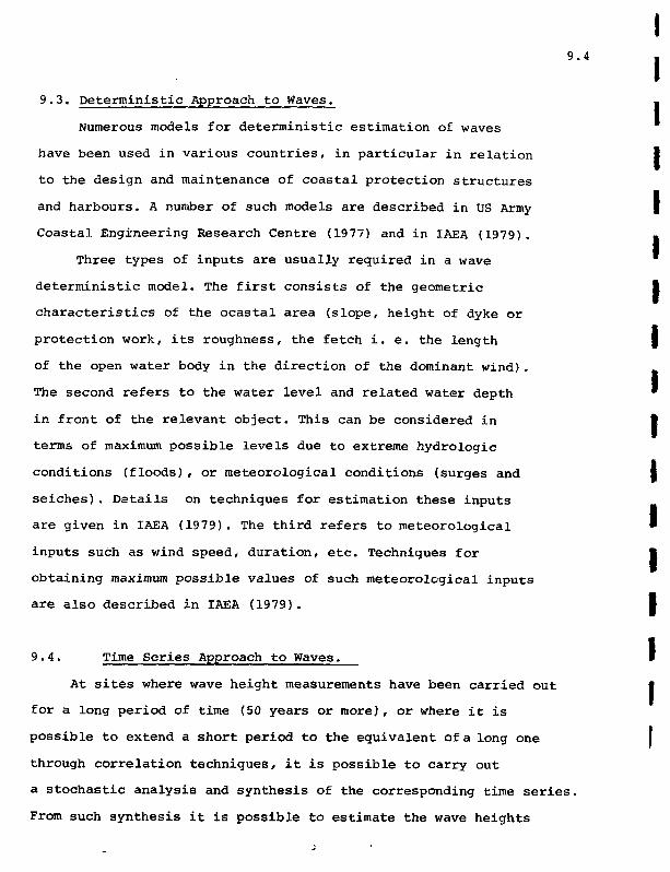
9.4

9.3. Deterministic Approach to Waves. .

Numerous models for deterministic estimation of waves

have been used in various countries, in particular in relation I

to the design and maintenance of coastal protection structures

and harbours. A number of such models are described in US Army |

Coastal Engineering Research Centre (1977) and in IAEA (1979). .

Three types of inputs are usually required in a wave

deterministic model. The first consists of the geometric 1

characteristics of the ocastal area (slope, height of dyke or

protection work, its roughness, the fetch i. e. the length f

of the open water body in the direction of the dominant wind).

The second refers to the water level and related water depth "

in front of the relevant object. This can be considered in 1

terms of maximum possible levels due to extreme hydrologic

conditions (floods), or meteorological conditions (surges and f

seiches). Details on techniques for estimation these inputs

are given in IAEA (1979). The third refers to meteorological •

inputs such as wind speed, duration, etc. Techniques for I

obtaining maximum possible values of such meteorological inputs

are also described in IAEA (1979). I

II

9.4. Time Series Approach to Waves.

At sites where wave height measurements have been carried out

for a long period of time (50 years or more), or where it is

possible to extend a short period to the equivalent of a long one I

through correlation techniques, it is possible to carry out

a stochastic analysis and synthesis of the corresponding time series.

From such synthesis it is possible to estimate the wave heights

9.5

with low probabilities of exceedance and the probability of the

"maximum possible wave height".

Before carrying out the analysis the data should be

checked for consistency. In particular it must be ascertained

that the data have been obtained at the same point, using the

same datum, and that the conditions at the measurement point

have not been changed. If this is not true, adjustments to the

data have to be introduced before the analysis, including

corrections for jumps and trends.

The methodology to be used is practically the same as for

maximum flows (3.2), with some minor differences. These are:

i) The original (i. e. the arithmetic) values of tile

recorded time series are used in the analysis, i. e.

the initial logarithmic transformation used in the

case of maximum flows is not required in this case;

ii) The ice cover period is eliminated from the analysis;

in connection with this it may be necessary to use

a seasonal autocorrelation coefficient.

REFERENCES

American Huclear Society (1976), American National Standard, Standards forDetermining Design Basis Flooding at Power Reactor Sites, ANS - 2.8, NASIN170-1976.

Amorocho, J., and Brandst^tter (1971), Determination of nonlinear functionalresponse models in rainfall-runoff processes, American Geophysical Union, WaterResources Research. Vol. 1, No. 5.

Anderson D.V. and J,P. Bruce (1958), The storms and floods of October 1954 inSouthern Ontario, Proceedings of IASH General Assembly, Toronto, IASH Gentbrugge,Belgium.

Bruce, J.P. (1957), Preliminary estimates of Probable Maximum Precipitation overSouthern Ontario, Engineering Journal, Vol. 40, No. 7, July pp 978-984.

Creager, W.P., J.D. Justin, and J. Hinds (1957), Engineering for Dams, JohnWiley & Sous, New York.

Fiering, M.B. (1963), Use of Correlation to Improve Estimates of the Mean andVariance, U.S. Geological Society, Prof. Paper 434C.

Fiering, M.B., and Jackson, B., (1971) Synthetic Streamflows, American Geo-phvsicalUnion, Water Resources Monograph 1, Washington, D.C.

Fread, D.L. (1973), A Dynamic Model for Stage-Discharge Relationships Affected byChanging Discharge, NOAA Technical Memorandum, NWS HYDRO 16, Silver Spring MD.

Gupta, S.K. and S.I. Solomon (1977), Distributed Numerical model for estimatingrunoff and sediment discharge of ungauged rivers, Part I, The Information Systai,Water Resources Research, Vol. 13, No. 3, pp. 613-618.

Huftschmidt, M., and Fiering, M.B., (1966), Simultation Techniques for WaterResource Systems, Harvard Univ. Press, Cambridge, Mass.

IAEA (1979) Safety Guide on Design Basis Floods for Nuclear Power Plants on RiverSites, Draft of SG10A, IAEA Vienna.

IAEA (1979a) Safety Guide on Design Basis Floods for Nuclear Power Plants on CoastalSites, Draft of SG10B, IAEA Vienna.

IAEA (1979b) Safety Guide on Meteorology - Extreme Meteorological Condition inNuclear Power Plant Siting, Draft of SG-S11, IAEA, Vienna.

Kartvelishvili, N.A., (1967), Theory of Random Processes on Hydrology and FlowRegulation (in Russian: Tiorya veriyatbistnyk processov v gidrologu i reguli-vovanii stoke), Gidemeteorologischeskoe Izadtel'stvo, Leningrad.

Kisiel, C.C., (1969), Time Series Analysis of the Hydrologic Data, Advances inHydroscience, Vol. 5, edited by V.T. Chow, Academic Press, New York.

Klemes, V. (1973), Applications of Hydrology to Water Resources Management, WorldMeteorological Organization, Operational Hydrology Report No. 6, WMO, No. 356,Geneva.

- 2 -

Kottegoda, N. (1970), Statistical Methods of River Flow Synthesis for WaterResources Assessment Proc. Institution of Civil Engineers, paper 73395, tondon.

Linsley, R.K., Kohler, M.A., Paulhus, J.L.H., (1975), Hydrology for Engineers,McGraw-Hill, New York, Second Edition.

Kouwen, N., Harrington, R.A., and Solomon, S.I. (1977), Principles of graphicalgradually varied flow model, Journal of the Hydraulic Division, ASCE, Vol. 13,No. HY5, May, pp. 531-542.

Natural Environment Research Council (1975), Flood Studies Report, London.

Nordin, C.F. (1976), Simulation of velocity distribution and mass transfer,Chapter 22 in "Stochastic Approaches to Water Resources", edited by H.W. Shen,Fort Collins, Colorado.

Paulhus, J.L.H. (1973), Manual for Estimation of Probable Maximum Precipitation,WMO Operational Hydrology Report No. 1, Geneva.

Sherman L.K. (1942), Hydrology, Part IX in "Physics of the Earth" edited byO.E. Meinzer, pp. 514-525.

Shocklitsch, A. (1917), Ueber Damnbruchwellen, Proceedings of the Vienna Academyof Sciences, Vienna.

Soil conservation Service (1974), Design of Small Dams, U.S. Department of theInterior, Bureau of Reclamation, A Water Resources Technical Publication, U.S.Government Printing Office, Washington.

Solomon, S.I. (1966), Statistical association between hydrologic variables,Proceedings of Hydrology Symposium No. 5, Statistical Methods in Hydrology,NRC, Associate Connittee on Geodesy and Geophysics, Subcommittee on Hydrology,Queen's Printer, Ottawa.

Solomon, S.I. and Associates Ltd., Application of Watmap-Watfile Data System toDevelopment of a Distributed Water Quantity-Water Quality Model for South NationRiver Basin. Report prepared for Water Resources Data Systems Section, WaterPlann. and Manage. Br., Environ. Canada, Ottawa, Ontario, Canada, March 1976.

Solomon, S.I. and Gupta, S.K. (1977), Distributed numerical model for estimatingrunoff and sediment discharge of ungauged rivers. Part 2, Model development,Water Resources Research, Vol. 13, No. 3, June, pp. 618-624.

Solomon, S.I., and Jolly, P. (1976), Regional Analysis of Maximum Flows forStreams Crossed by the Proposed Artie Gas Pipeline, The Shawinigan EngineeringCo. Ltd., Montreal, Canada.

U.S. Coastal Engineering Research Centre (1977), Shore Protection Manual, ThirdEdition, Ft. Belvoir, Va.

U.S. Nuclear Regulatory Commission (1977), Regulatory Guide 1.59, Design BasisFloods for Nuclear Power Plants, Revision 2, August 1977-

World Meteorological Organization (1969) Estimation of Maximum Floods, Tech.Note No. 98.

- 3 -

World Meteorological Organization (1975), Intercomparison of Conceptual Models,Used in Operational Hydrological Forecasting, Operational Hydrology Report No. 7,WMO Publication No. 429, Geneva.

Yevjevich, V. (1972), Stochastic Processes in Hydrology, Water Resources Publica-tions, Fort Collins, Colorado.

Yevjevich, V. (1976), Chapters 1 to 4 in Stochastic Approaches to Water Resources,H.W. Shen, Editor and Publisher, Fort Collins, Colorado.

TABLES

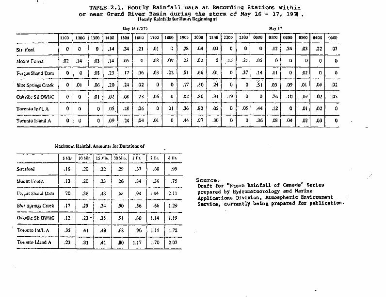
TAELE 2 . 1 . Hourly R a i n f a l l Data a t Recording S t a t i o n s w i t h i no r near Grand River B a s i n dur ing t h e storm of May 16 — 17 , 1971 .

Hourly Rainfalls fur Hours Beginning at

Stratford

Mount Foicjt

Fuifus Slund Dam

Blue Springs Creek

OakvJlc SE OWRC

Toronto Int'l. A

Toronto ldar.d A

1)00

0

.02

0

0

0

0

0

1200

0

.14

0

.01

0

0

0

1300

0

.OS

.OS

.06

.01

0

0

1400

.14

.14

.23

.20

.02

.05,

.09

May 16 <1:S7)

1500

34

.05

.17

.24

.08

.28

.24

1600

.2)

0

.06

.02

.23

.06

.04

1700

.01

.OS

.03

0

.06

0

.01

1800

0

.09

.22

0

0

.01

0

1900

.28

.23

M

.17

.02

.36

.44

2000

.04

.02

.66

.30

.80

.82

.97

2100

.03

0

.01

.24

.34

.OS

.30

2200

0

.15

0

0

.19

0

0

2300

0

.21

.37

0

0

' .05

0

0000

0

.05

.14

110

.44

.36

May 17

0100

.12

0

.11

.09

.26

.12

.08

0200

34

0

0

.09

.10

0

.04

0300

.03

0

.02

.01

.02

.01

.02

0400

.22

0

0

.06

.02

;Q2

.03

0500

.07

0

0

.02

.05

0

0

Maximum Rainfall Amounts for Durations of

Sirail'oru

Mount 1-oresl

VttMi SliunU Dam

Blue ipr/ngs CY.'rk

Oakvitla SF. OWUC

Toronto Ini'l. A

Toronto JsJand A

5 Min.

.16

.13

20

.17

.12

.35

.23

10 Min.

.20

.20

.36

.25

. 2 3 -

.41

31

15 Mi...

.22

.23

.48

.34

.35

.49

.41

30 Mlu.

.29

.26

.68

.50

.51

.68

.80

1 llr.

.37

.34

.94

.56

.80

.90

1.17

2 !!.-.

.60

.36

1.44

.66

1.14

1.19

1.70

i Mr.

.99

.75

2.11

1.29

1.19

1.7S

2.07

Source:Draft for "Storm Rainfall of Canada1 Seriesprepared by Hydrometeorology and MarineApplications Division, Atmospheric EnvironmentS«rvic«, currently being prepared for publication.

Page 1 of 3

TABLE 2.2. Maximum Mean Daily Flows of Grand Riverat Gait (cfs).

Recorded Values

Vear

O2GA003 13

02GA003 14

02GA003 t"J5~

Monthly maximums

First line: January to June; Second line:December

July to

AnnualMaximurr

02GA003 16

02GA003 17

02GA003 T8"

02GA003 19

02GA003 20

02GR003 21

02GA003 22

02GA003 23

O2GA003 24

02GA003 25

02GA003 26

02GA003 27

02GA003 28

02GA003 29

~O2GflOO3 30

02GA003 31

02GA003 32

020ft003 33

185.002880.00265.00

• 610.00945.00

13700.00530.00680.00

10500.00•- 373.00

264.002040.00182.00270.001690.003610.003200.00835.00455.00188.00390.00

-2800-. 0O~473.00195.00195.00875.00170.00

—"441.00-6190.001290.004010.001430.00880.00

2030.00307.00126.00795.00

340.00 210.00 395.002250.00 '1700.00 9050..00432.00 490.00 272.00

2890.00 5550.00 9930.004370.00 8790.00 2630.009250..00 19700.00 15100.00154 ,.00 190.00 460.00420.00 25400.00 10800.00656.00 248.00

9310.00 17400.00210.00 1530.00695.00 24200.00203.00 301.00240.00 16200.00

253.00

2720,1.300..1030,

3950,4740.4 00,

3070.750,

1130.1530.3930.5760.1280.

415.001590.00 14200.00440.00 225.00

660.009350.001450.009510.00570.00

7-840.00750.00

8560.002400.00

4390.00 12500.00 19000.00770. ">

8560412.00 350.00

390.00 10800.00 16100.00560.00 402.00 1250.00

6280.00 16700.00330.00

8840.00 14500.002460.00 3040.00 13000

435. 00 20SO0V00 4320. 00" 531O"462.00 207.00 625.00 2820

.00 26800.00 15500.00500.00 2090.00

610.00 26900.00 29700.00211.00 130.00 545.00

3930T0O 11400.00151.00 174.00

4280.00303.00

00000000000000000000

485.. uO300.00

L670.00398.00

UiVO.OO5 340.00

530.002 520.. 00510.00530.00

00 10200.000000000000

1.360.003020.001060.006480.001570.00

380.00158.00217.00

203.00935.00

5760.00

68E1860.00

337.00,0 17600.00 10800

5307880335

5200.00 485910.00 7250

4430

56004180.00 13200.00920305

3160.00177.00136.00239.00

6630.00199.00

18300.00 23100.00 11800.00 11100.00465.00 2030.00 8020.00 1860.00

K> "775.00 "195.00 151.00

H> 13300.00136.00 170.00

13106830519010405290181.

1440.2340.1840.7390.4180."

985.

,00.00,00.00,00.00,00,0000,00roc,0000,0000,00xxr,0000

2060.00425.00

1410.005330.00905.00580.00157.00

4010.002200.001760.0033X0700" -3030.00840.00

2070.00735.00273.00

—427.00-195.00423.00

00 12400.0000 1930.0000 2100.000000 v/u.uu

680.00

2 " , * > ' • > •

1740 1 •

2.4'j*. .

! 6'J'.-'-

.14'..: 00

19000

174.00

16100

16700

14500,

20600,

26800.

29700.

11400.

12400..

23100.

15500.

2 of 3

I1

Table 2.2. Maximum Mean Daily Flows of Grand River at Gait

(cfs)

Recorded Values

Year

02GA003 34

02GA003 35

Cr2Gfi003 36

02GA003 37

02GA003 38

39

Monthly Maxi.miimsFirst line: January to Jur.er S O C O M I

02GA003 40

02GA003 41

O2GAOO3 "42""

02GA003 43

02GA003 44

020A003 45-

02GA003 46

02GA003 47

02Gft003 48-

02GA003 49

02GA003 50

02GA003 51

02GA003 52

02GA003 53

02GA005--54-

02GA003 55

02GA003 56

O3GAOO3-S-7-

965.00133.00590.001260.00201.. 0097.00

4230.00423.00175.00170.00

-1380.00640.00106.00

1500.001200.00370.00

- 640.00675.00

2890.00925.00

2890.001220.00-515.004240.00

11200.00735.00

4200.007290.00

—505.00"1330.007330.00642.00

12900.001020.00

13600.00 -1750.005980.001060.003040.003210.00-654 ."O0--550.00

4400.00472.00839.00

2240.00-5540.-006080.00

31090

455157

,<1 3..77 .

3180.409.

16100.1810.1130.233.118.

2630.500.560.460.263.

8670.1000.1040.990.490.840.

1830.640.

1950.1190.

- 781.395.

5560.410.

1350.915.

6020.608.

3670.460.

5150.1210.

tsooo.708.691.613.510.

20400.961O.680.

. 00 2820.00

.00 142.00

.00 18600.00,,00 87.0000 13200.0000 188.0000 1180.0000 207.0000 19800.0000 825.0000 13200.0000 151.0000 320.0000 2420.0000 3140.0000 405.0000 20300.0000 6480.0000 22300.0000 920.0000 13400.0000 630.0000 16800.0000 2700.0000 18700.0000 590.0000 7830.0000 1010.0000 37700.0000 360.0000 23200.0000 340.0000 22500.0000 580.0000 i8500^0000 602.0000 10700.0000 415.0000 9330.0000 504.0000 17200^0000 555.0000 10300.0000 422.0000 7710.0000 6640.0000 483O.OO00 1060.00

1.3200. <;o184.00940.00.1.36.00

'3030,00

12100.00725.00

4690.00207.00

23100.00209.00

2.1.200.003200.00

13700.00870,00

8620.002760.00

25600.00900.00

13200.00580.00

9640.006000.00835.00600.00

36800.00485.00

407O.00193.00

4410.00894.00

26800.00841.00

162O0;OO-3700.00

13500.00340.00

5730.00498.00

17800-.0O40300.009860.00630.00

23100.001610.00729O.OO1790.00

• : J:.'

073,1)0445.OuL410.00II? 7 0.00C*40.00i4^0.004000.00535 ,,001630.00347.00

1600.00325.00

Y740.007370.00560.00

2410.0014100.0010900.0024100.002020.003470.00525.00

13700.002220.001.250.00530.00

10800.00480.00

226O-.OO2180.00619.00295.00

1460.003210.00

Annua10--n. ftexin.ur

:>vi.

11500.00390.00

520. <:-:•3fil .00355 ..00373.00590.0024 :t .00

3620.- <">20400.00

440.006110.00

14 000.004250.001640.00650.00

1960.00430.00

4140.00970.00650.00

2300.0022200.002050.00

430.00460.00

13000.001640.0010700.00

12800.001940.00999.00

12600.00548.001710.OO-2110.002140.003470.00

21700.001430.00

3990.00580.00

4560.006060.00575.00

—8S+-.W--3770.00839.00

2390.001190.004270.00

12000.004230.00 14000.00

12100.. •

2 1 ~-<.<v.. '•

1 7 - ' 0 ' 1 •

2030< .. •

13400.'.-

18700.0

36300,, 0

37700.. 0

23200.. 0

26800.0

18500.. 0

13500,. 0

12600.0

40300.0

10300.0

23100.0

14000.0'

Page 3 of 3

Table 2.2. Maximum Mean Daily Flows of Grand River at Gait

(cfs)

Recorded Values

Year02GA003 58

026A003 5?

•02GA003-6O-

02GA003 61

02GA003 62

Tirst line: .7 a

02GA003 64

O2GA003 65

02GA003 66

02GA003 67

02GA003 68

TOO 4 6y

02GA003 70

02GA003 71

02DA003 73

02GA003 74

02GA003 73

1770.001000.00815.00910.00

-l~280 s 00-1180.00211.00839.00467.00679.00

—582.00652.00

1410.001080.003460.00668.00

5700^00613.00

6760.007680.003770.001310.004ti60."00~980.00520.001080.001440.001440.001300.00"1380.003440.00728.00

6410.00918.00

1870.00809.00

1400.005140.00700.001700.00999.00696.00

560.540.995.803.

-1360.917.

6110.987.296.657.

-- 559.662.743.

2170.16600.486.

Monthly Maximumsnuary to June; Second linu

00 394§.00r 2300.00

6022270103086005220~4"45011905878171370144073O860563012102610645

5880538053701220400133093D757

000000000000000000000000000000000000000000000000000000

565.00 340.005370.00 17300.00743.00 3050.00620^00 240GO.00

858.002970.00662.006300.00

725174031506710

779.002880.00917.00

11000.005B1

. 0 0

613.003380.00785.00

931.00

. 0 0

1010.3240.1050,749.3240.

00000000

0000000000

675.00560.00790.00

3550.00

422.001830.001750.001080.002220.00

4490.00571.00

5050.00 14000.00520.00 3510.00

571.2030.565.

6090.6000,

3340.00 3070.4060.00624.00 576.00

6710.00 23200.001500.00 5430.009040.00 4620.003550.00 2260.00

™ — ' ~Z0VT. 0 0611.00

U03O589.001910.001140.00

8050.001270.00

2780.00 12200.00670.00 594.00

00 2300700-00 854.0000 15300.00

1490.1570.4670.1110.9340.T9MT.2020.2580.2330.1580.

472.

0000000000•03-0000000000

w0000000000

376.00852.00

3570.00640.00

6560.00

Annual:. .y.:. urn

3V40.0'/

17300., 0'

24000.. 0<

6110.0'

11000.0'

12400.0c

4490.. <>•

16600 .0 '

00 721.00

2300.008960.00926.00

1940.3130.

.00 13500.00 14600.00 3020000 716.00 713.00 1460

oooooo00,00

6310.007 730.00liOOO.OO1360.006150.00~9wnnr580.00761.00

3940.001990.001980.00

"T430.002780.002480.001840.001410.00564.00

7X3X3 633U.UU.00 1340.00,00 17700.00

2500.0015700.003550.00

6310.. 0'.

'23200.Gi

9340.0<

17200. 0'.

8050. C"

12200.(>•

25900.0

15300.0

30200.0

02GA003 76

02GA003 77

02GA003 78

,000000

70X3 ~,00

890.005770.001980.004090.004840.00

1360.6580.1800.755.

3300.

0000000000

3800.001490.001260.00593.004600.00

19800.0

17700.0

15700.0).UU

1780.007KT 4100 .

947.00 1190. 00/z/.uu

1320.00 15100.0

TABLE 2 .3 . Maximum Mean Daily Flows of Grand River a t G a i t .Ccfs)

veer -'••••.Til 4 0

fi.-ii.rNi 41

riALTMl 42

C3ALTN1 43

OiV.TNl 44

oALTNl 45

3ALTN1 44

GALTNI 47

GALTNI 4B

GALT;<1 4?

GALTNI SO

0ALTN1 51

GALTN1 52

C-ALTN1 53

0ALTM1 34

GALTNI 53

GALTNI 54

QflLTNl 57

<5ALTN1 53

GALTNI 59

GALTNi 60

GALTN1 61

GALTNI 62

GALTNI 63

GALTNI 64

QALTN1 65

GALTNI 44

GALTNI 47

GALTNi 63

GALTNI 49

GALTNI 70

GALTNI 71

GALTNI 72

GALTNI 73

GALTNI 74

QALTN1 75

Deregulated FlowsMonthly Maximums: First line: J-second line: Jul" to rwcemher-' 10.5.00 * 113.00 "' 32O.OO-.ILJOO- 1S-.10.00 i 2630.00 : 2420. Vr ~2'.-1-1200.00 300.00 1140.30 :3i',:

S6O.00 405.00 s?o460.00 23055.00239.00 7213.00

370.00440.00731.002190.001020.003-147.001143.00441.00

2S7A3670.00 24327.00 2372i

636.001540.00 870.00735.00 13391.00 17S2-).770.00 261.00 263.490.JO 23609.00 T'.J<sS.

4234.00 337.00 2705.00 OJ'C.llaOl.OO 1330.00 20162.00 -31,-93.00 506.00 237.00 532.

4317.00 1940.00 7331.00 37233.71T3.00 923.00 905.00 376,505.00 781.00 44040.00 5711.1044.00 115.00 217.00 17i.7341,00 5574.00 23222.00 2306,563.00 222.00 199.00 952.

12915.00 1270.00 27375.00 27537.997.00 927.00 350.00 75B,

13434.00 4020.00 23355.00 14902.1681.00 416.00 402.00 3S;46190.00 3667.00 10957.00 14al3,771.00 326.00 413.00 342

2S50.00 4990.00 10654.00 3739.3225.00 1131.00 411.00 240643.00 12913.00 13295.00 13527.413.00 350.00 533.00 4S7SC,

4571.00 700.00 10403.30 11943,225.00 512.00 282.00 493790.00 506.00

2531.00 20792.00 ".1132.005423.00 9610.00 6536.00

540.00535.00611.00997.00696.001582.00797.00

4904.00673.00

nuary cc June ."'T.;i

: • ! - - 7 4 0 . O J j j . - _ • . . •

00 540"c-5" " '••'-' '. ':vC 2 4 . 0 . V . . 4 1 - : . j 'C<3 U 5 S 3 . 0 0 :~il?~ .::•-

3430.00 :ia;'.'. ..4S3.0C 3--;.iC

13721.03 4:^4. ..21^'.oj .> .-;:

A459.00897.00.W9.00327.00534.001276.001037.00220.00639.00329.00437.00393.00501.001602.00844.00

7733.00 2760S9737430

983.00 19955849.00 4E44S71.00 325

4916.00 235101053.00 23304247.00 39508333.00 421

6583.00 3225724.00 313

293.00 17680.00 14713502.00 304.00 90B

3500.00 9650276.00 284

5501.00 10090445.00 247

3387.00 16744240.00 5174

9423.00 7023.00 3093.00 30542"5.00 337.00 317.00 333

13477.00 1695.00 13235.00 278403221.00 2090.OC 1351.00 893E1335.00 10254.00 12853.00 53841112.00 4936.00 42E3.C0 37194827.00 4370.00 11574.00 17370778.00 762.00 239.00 48S517.00 639.00 1914.00 14749104B.00 472.00 861.00 13311111.00 1342.00-- 3179.00 193551406.00 1177.00 392.00 3551453.00 779.30 2299.00 303541121.00 463.00 449.00 21944708.00 5583.00 13925.00 6532530.00 1332.00 396.00 7438328.00 4216.00 23420.00 19130728.00 336.00 409.00 4593329.00 5861.00 7320.00 309006O2.«O 5042.00 1416.00 868

406.00414.00737.002806.00

3653.00 16744.00417.00 256.00

7023.00337.00

S0 7.CC11497.00442.00

2271.00002217

721.00232.00

3136.CC2230.301320E.OD2239.00-.063. CO

12972.30556.00

2173.002132.0-:2058.003654.00

00 21616.0000 1590.0000 1756.00

5025.00750.001763.004327.003322.0017440.001096.00

•3576.001053.00773.00

1313.004130.00466.00

2104.00472.00

5900.006455.003173.001663.001363.002594.002116.00

CO 11290.0000 7380.0000 2417.00

3054.003414.001323.00369.00

3127.002304.004105.003X26.00

00 30142.0000 1522.0000 3335.00.00 1354.00

2300. C •:22344.002145.0"1U3.5:495.00203.<V)

23240.001927.001067S.001273.Ou3492.00

,0000.00

:o000000

,0000.00,00.00,00.00,00,00iCi,00.00,0000.0000,00oo.00,00.CO00

00,00,00,00,00.00,00,00

" 3 ? . - •

44040. :•(•

1293.00166S.0C

12333.CO21450.00

425. 0.)5«4.C0771.CO

3702.OC2977.O'",374.00

2190.002223.0?'71.J0

3311.00530.00264.OC781.00

4212.00499.00

9040.004372.009874.007850.0012379.001063.007530.00771.00543.00414.00

5285.002094.002667.0019S9.003003.002003.00297E.001213.00449.50

2792.006220.00

23510. •>(•

3*503.30

l"4J->. :•>

23500.00

10090.00

is7£.;.oo

?3?'-.. V:

Z~ri't J- O'J

17370.0

1494T.0&

19355.0"

30354.Ot

13925.00

30142.00

30900.00

MtTtt SURVEY OF CANADAAUG 3 1979 PAGE 211

GRAND RIVER AT GAIT

Page 1 o f 2

STATION NO. 02GAQ03

< CUELPM. ONT

, 1915> 1916I 1917. 1914I 1919

| 19201921

! 1922I 1923;' 1921.i{ 1925'> 1926i 1927

192 41929

I 193 0

ANNUAL EXTRC1ES OF DISCHARGE I N CFS ANO AHNUAL l O f A l DISCHARGE I N AC-FT FUK THE PERIOD OF RECORD

HAXIMUH INSTANTANEOUS DISCHARGE

1932| 1943"I 193I|

! 1935' 19 36

! 1938"| 1934

. 191.0191.1191.2

I 191.3! 191.1,

' 191.5; 191,6

i IV,», 191.9

< 195 0I 1951I 1952

195.11 195l|

' 1955

195?195 3195')

MAX I HUM OAILV OISCMARGE

11700 CFS ON MAR 28

8430 CFS ON APR 1119700 CFS ON I1AR 3025400 CFS ON MAR Ik17U00 CFS ON MAR 22 "21.200 CFS ON MAR ID

16200 GFS ON IMR 1311.200 CFS ON MAR 919O0O CFS ON APR 12 _17600 CFS Oil APR 716100 CFS ON APR 6

16700 CFS ON MAR 1911.500 CFS ON APR i i20600 CFS ON HAR 1".26400 CFS ON MAR 25"'~29700 CFS ON APR 6

13000 CFS AT 1130 EST ON APR 7

31700 CFS AT 1130 EST ON FEQ 1217200 CFS * T 0630 ESt 'ON APR 219300 CFS AT 1900 ESt ON APR <»

20200 CFS AT 2300 E S I ON HAR 1716300 CFS AT <M3d ESI ON HAR 2a16D00 CFS AT 2000 E S I ON APR 6231.00 CFS AT 1300 E S I ON HAR Zi .27000 CFS AT 0700 EST ON APR 19

21.1.00 CFS AT 0900 EST ON APR 916200 CFS AI 1330 EST ON APR 735900 CFS AT 1500 ESI ON HA? 1733000 CFS AT 0800 F.ST ON HA» IZ29900 CFS AT 1030 EST ON HAR 25

19200 CFS AT 2100 EST ON MAR 1630200 CFS AT 1700 EST ON MAR 7MMO CFS AT 1300 EST ON APR 121,6300 CFS AT 0900 EST OH HAR 20301-00 CFS UN HAR 23

30600 CFS AT 0200 E S I ON APR 523100 CFS AT 0500 EST ON HAR 3117300 CFS AT 0400 EST ON APR 219100 CFS AT 1800 E S I ON MAy 261.9000 CFS AT 1>.OO EST ON OCT 16

15<>ac CFS AT 2 3 0 0 E S t ON MAR 113 V 5 J 0 CFS AI 1500 EST ON HAY 1215400 CFS AI 1730 ESI ON OtC 21•.140 CFS AI 1500 ESI ON HAR 29

20100 CFS AT 10011 ESI CN APR 6

r.rs A! OH

11",Of) CFS ON APR 712<>00 CFS ON DEC 252 3 1 0 0 CFS ON FEB 121 5 5 0 3 CFS ON APR 2 '15 20'') CFS ON APR i.

1 4 6 0 0 CF5 ON HAR 171 3 2 0 0 CFS ON HAR 2912100 CFS ON APR 61 9 9 0 0 CFS ON NAR 21."2 3 1 0 3 CFS ON APR 19

2 1 2 0 0 CFS ON APR 91 3 7 0 0 CFS ON APR 72 0 3 0 3 CFS ON MAR 172 5 6 9 3 CFS ON APR 213I.0Q CFS ON nAR 25

16/100 CFS ON NAR 171H700 CFS ON HAR 73 6 4 0 0 CFS ON APR 123 7 7 0 0 CFS ON HAR 202 3 2 0 3 CFS ON HAR 23

2 6 4 0 0 CFS ON APR 519500 CFS ON HAR 311 3 5 0 0 CFS ON APR 212oOO CFS ON HAY 3 'i ,03i)0 CFS ON OCT 16

10300 CFS OH HAR 1223100 CFS ON APR 5mOOO CFS DM OEC 21

34U0 CFS ON HAR 2917J00 GF.J OH APH 6

?•»os i r.F -, on ftp-? >

MIHIMUH DAILY DISCHARGE

55.0 CFS ON AUG 9

131. CFS ON JUN 27

'12.a CFS ON SEP 26!<,•, CFS ON SEP 30

65 .0 CFS ON AUG 1456 .0 CFS ON JUL 19

81 .0 CFS ON SEP 690 .0 CFS ON SEP 1175.0 CFS ON AUG IS77.0 CFS ON AUG >

109 CFS ON NOV 8

1.9.0 CFS ON JUL 19 5 . 0 CFS ON AUG 15

_ 127 _ CFS ON AUG 21" 106' "CFS ONSEP" 2

55 .0 CFS ON SEP 8

5 7 . 0 CFS ON AUG 26 9 . 0 CFS ON SEP I I

I3i) CFS ON JUN 2734.0"' CFS OH SEP 21.29 ,0 CFS UN SFP 3

36 .0 CFS ON AUG 3126.0 CFS ON AUG ) "6 7 . 0 CFS ON JUL 2".9 7 . 0 CFS OH OEC l i .77.0 CFS ON JUL 2 t

85 .0 CFS ON AUG 177 3 . 0 CFS ON SfP 24

100 CFS ON SfP J173 " CFS ON OtC 231 2 1 CFS ON JAN 19

169 CFS OH AUG 6112 CFS OH OCT 52 5 8 CFS UN OEC 1

4 4 . 0 CFS ON OCT 7158 CFS ON NOV 26

21.63 3 113025 7 '2 9 7

2 2 13172 9 12 2 2356

CFSCFSCFSCFSCFS

CFSCKSCFSCFSCFS

ONONOHUNON

ONONOHONON

AUGAUGacimeJ&N

or, iFEB

ocrAUGJAM

1213I t17I S

t .

2 111241 £

TOTAL DISCHARGE

1.53000 AC-FT

71.1000 i967 0 00 ,

835000 i457000756000

7170008390007770007960007920 00

6820801200000

91,2000105000111050000

822003510003

1150000672000660000

527000576000B9UO0O71600.1733000

977000663000

1080009" - 1.270000

6920D0

1060000

69300011.30003

91400081000]

1 11,00001310000

879(100912000

12100011

9530001270000

91.5000L ? 7 1 .1.1

AC-FIAC-FTAC-FT.hC-FTAC-FT

AC-FIAC-FTAC-FTAC-FIAC-FT

AC-FTAC-FTAC-FIAC-FTAC-FT

AC-FTAC-FTAC-FIAC-FIAC-FT

AC-FIAC-F rAC-FTAC-FTAC-FT

AC-FTAC-FTAC-FTAC-FTAC-FI

AC-FTAC-FIAC-FfAC-FTSC-FT

AC-FIAC-FTAC-FTAC-FTAC-FT

AC-FIAC-FTAC-r isr.-FI

re A«

19 m

1,15191619 17 .19181919

192 01921J92219231921.

19251926192719281929

193019311932195 31931,

1935193619.5 719381939

191.019ii 1191,2I9t*i191. i.

191.5191.6191*7191.8

1919

195019511452195 11451.

145019^61957195 1

•)9f.0 0) AC-F I

CFS 'in 0' C i 3 • ) : )

TABU: 2.«

H»TE* PURVEY OF CtNAna GRANO RIVER AT GAU SIATIOH NO.AUG 3 1979 P«GE 212GUCLPH, ONT ANNUAL EUHCME5 Of DISCHARGE I N CFS «NO ANNUAL IU11L DISCHARGE IN AC-F I FOR IME PERIOU OF «ECORO

TEAR HAXIMUN INSTANTANEOUS DISCHARGE

1 9 6 1 6 6 9 0 CFS AT 1 1 0 0 EST ON FER 2 41962 UaOD CFS AT Dn 3D EST OH "AU 301963 m o o CFS AT 0100 I-ST ON MAR 36196i< 5730 CFS AT 1500 EST ON Al'R 8

1965 25100 CFS AT 0730 EST ON FEB 111966 7750 CFS AT 1700 EST ON DEC 71967 30800 CFS AT 12U0 EST ON APR 3196» 121(10 CFS AT 1U30 fST ON HOY 291969 2*UO0 CFS AT 0U29 EST ON APR 19

1970 ""»»ID' CFS AT 02C «. LSI ON APR 171S71 13300 CFS AT 0355 EST ON APR lfc197? 30100 CFS AT 15<«S EST ON APR 191973 17300 CFS AT IU.20 ESt ON H«R 121971. 51.&00 CFS AT 1719 EST ON HAY 17

1975 30100 CFS AT 1625 EST ON APR 191976 20900 CFS AT 1536 EST UN MAR Zi.1977 20300 CFS AT 1732 EST ON MAR 131S7« 16000 CFS AT 052.5 EST ON APR 1".

H«>IHUM DAILY niSCHtRG

6110 C " n« FEB ZU11000 CFS ON MAR JO12<t00 CFS ON Mil !h

kU10 CFS ON APR «

16600 CFS ON FEB !16310 CFS O N nrc 6

23200 CFS ON Al'R X93<<0 CFS ON HOY ?9

17200 CFS ON A?R 19

»050 CÎS OH APH 1212200 CFS ON Al'R lu25*300 CFS ON APK 1915-300 CFS ON HA* ]Z30200 CFS ON «AT 17

19S00 CFS ON APR 1917701) CFS ON MAR 2i15700 CFS ON (1AR 1315100 CFS ON APR I «

MIHI^UH DAILY DISCHARGE

155 CFS ON JAN 212S8 CFS OH JUL 21231 ' CFS ON OCT 19Î38 CFS ON NOV 22

•J.'l CFS OH JUL 133U0 CFS ON NOi/ ?1*5 CFS OH A1IG 23- 2 7 CFS ON JUN ^132» CKS OH OEC 2

;»<•JZ9•.ZJ330329

317U7826»

CFSCFSCFSCFSCFS

CFSCFSCFSCFS

ONONONONON

ONOHOHOH

JANDFCOFCOFC

me

JANJUNJANAUG

2625

ii.!7

61331m

TOTAL DISCHARGE

Paye 2 of 2

YEAR

5710005550D0566C00515000

1090000726000

138000311100001030000

79900079900097 00 00

10600001070000

97600012500001060000

SH50O0

AC-FTAC-FT«C-FTAC-FT

AC-FTac-rrAC-FTAC-FTAC-FT

AC-FTAC-FTAC-KIAC-MAC-FI

AC-FTAC-FTAC-FTAC-FT

19611S6Z1963196U

1"6519&6l i f .7195Ï1969

1970197119721973197U

1975197619771S7»

• - EXTREME RECORDED FOR THE FIRIOD OF KECORO AC-FI HE AN

TABLE 4.1. PMP Estimates for Grand River t Gait

(inches)

Column No.

Duration ofPMP (hours)

2

From Bruce (19 56)

For 1350sq. mi.

For 10sq. mi.

Thun- Tro- Thun-der pical derstorms storms storms

From SCS (1975)

For 1350 For 10sq. mi sq. n.i

IIIIII

10.2 7.0 16.1 12.0 25.1

12 10.8 10.4 16.7 13.8 27.6

24 11.2 11.4 17.4 15.' 30.1

III

TABLE 4.2. Gr£>r/5 river r.t Gait.

ESTIMATE OF FLOW AT GALT ASSUMING RELEASE OP WATER

FROM SHAMD AND CONESTOGO DAMS EQUAL TO INFLOW IN RESERVOIRS

1Hr

1

2

3

4

5

6

7

8

9

10

11

12

13

14

15

16

17

18

1$

20

21

22

23

24

2ShandLag-17h

2200

2100

2000

1900

1860

1820

1780

1770

1769

1780

1783

1786

1790

1797

6800

9577***

9520

8875

6665

7000

6500

6300

6200

6200

3W.Mont.Lag=Uh

2650

2670

2710

2740

2770

2860

3000

3150

3520

4210

5660

7840

10400

16500

20400

23000

24300

22900

21300

19700

18100

16600

15000

1310C

4G.AllenLacj=13h

1000

900

870

840

810

780

750

720

700

4200

7700

11500

10600

9012

14000

15892

14850

15200

14900

14635

5200

6900

1750

2450

"LOWS

5Speed

Lag=10h

562

629

657

665

809

1140

1300

1340

1370

1400

1660

1890

2120

2450

2780

3120

3520

4100

4660

5200

5730

5990

6010

5876

IN C

6Canag.Lag=9h

1150

1460

1990

2680

2870

2970

3040

2940

2770

2610

2400

2210

2010

1820

1690

1610

1540

1450

1250

1030

824

651

532

434

PS

7Shiund 1Shaiiri 0

-170

-270

-370

-470

-510

-550

-600

-610

-621

-610

-607

-614

-640

-703

+3870

+1647

-780

-1435

-3165

-2150

-2320

-1950

-2030

-2000

bW.Mont.Ccrroc-ted

2480

2400

2 340

2270

2260

2310

2400

2540

2899

3600

5053

5126

9760

15797

24270

26847

23520

21465

18135

17550

15780

14650

12970

11100

9

•'•Q

4274

6124

6556

8130

7920

9083

9414

9460

8950

8110

8220

8620

9250

11700

13190

12390

11400

10990

10190

9440

8700

7980

7100

5950

GrantEstiatr.-i

ro 'i.

r)4<S*

1 1 5 1 •

1 2 3 i'

14581:

1466s:

16283

16904

17000

16689

19920

25032

29346

33740

40779

55930

57589

54830

53205

49135

47850

36234

36174

28362

25600

* Interpolation between the value of 11777 at 2245 and 6844 at 2320, May 16, 1974

** An averaqe of the two readinqs at 2320 and 0015, May 17, 1974

\Gtc:

Column 7: Inflow - Outflow at Shand Dam, con- .ion to be appliedto West Montrose flows to obtain deregulated flows there

8:- Column 3 - Column 7

9: Estimated inflow from ungauged area above Gait

1 0 : C o l u m n 4 + 5 + 6 + 8 + 9

TABLE 6.1A

Major Statistics of Annual Maximum Mean Daily Natural (1914-41)and Regulated (1942-78) Flows of Grand River

at Gait (Cambridge)

(for flows in cfs)

Period Mean (cfs)Value St. error

St. Deviation (cfs)Value St. error

Coef. of Skew Coef. of kurtossisValue St. error Value St. error

1914-41

11142-57

1958-78

17,787 983

21,975 2,28b

14,850 1,612

5,113 695

9,408 1,1.15

7,209 1,139

0.51 0.47

0.83 0.63

0.33 0.55

2.99 O.94

3.17 1.26

2.9 4 1.10

TABLE 6. IB

Major Statistics of Annual Maximum Mean Daily Natural f1914-41)and Regulated (1942-78) Flows of Grand River

at Gait (Cambridge)

(for logarithms of flowin efs)

Period Mean St. DeviationValue St. error V^lue St. error

Coef. of Skew Coe*. of KurtosisValue St. error Value St. error

1914-41

1942-57

1958-78

4 . 2 3 3 0 .024

4 .307 0 .047

4 . 1 1 3 0 . 0 5 5

0 . 1 2 6 0 . 0 1 7

0 . 1 8 0 0 . 0 3 3

0 . 2 47 0 . 0 3 9

- 0 . 1 1 O . 4 7

-0 .22 0.fi3

- 0 . f i ?. 0 . 5 •->

2.9.1

I'.faC

TABLE 6.2A

Major Statistics of Annual Maximum Mean Daily Natural (1914-41)and De-regulated*(1942-75) Flows of Grand River at

Gait (Cambridge)

(for flows in cfs)

Period Mean St. DeviationValue St. error Value St. error

1914-41 17,787 983 5,113 695

1942-57 25,436 2,548 9,840 1,301

1958-75 19,797 2,253 9,294 1,593

1914-75 20,34-1 1,066 8,327 753

Coef. of SkewValue St. error

0.51 0.47

0.86 0.6 3

0.39 0.59

0.97 0.31

Coef. of KurtosisValue St error

2.99 0.94

3.78 1.26

3.oo l.r-i

4 . J 2 0 . f>\

*Note: De-regulation means correction for changes in storaje

TABLE 5.2B

Major Statistics of Annual Maximum Mean Daily Natural (1914-41)and De-regulated* (1942-75) Flows of Grand River

at Gait (Cambridge)

(for logarithms of flow in cfs)

Period Mean St. Deviation Coef. of Skew Coef. of Kurtosis

Value St. error Value St. error Value St. error Value St. error

1914-41 4.233 0.024 0.126 0.017 -0.11 0.47 2.87 0.94

1942-57 4.376 0.042 0.166 0.030 -0.04 0.63 3.31 1.26

1958-75 4.244 0.056 0.231 0.040 -0.59 0.59 3.18 1.1°

1914-75 4.273 0.023 0.180 0-.D16 -0.30 0.31 2.50 0.C2

*Note: De-regulation means correction for changes in storage

Major Statistics of Second Order Differences for

a Time Series Based on Four Seasons

Grand River at Gait

TABLE 6.3

Period Coef. ofCorrelation

Standard Deviation Coef. of Skew\Talue St. error Value St. error

Coef. of KurtosisValue St. error

1914-74 0.175

1914-41 0.175

1942-57 0.044

1958-75 0.244

0.430

0 . 4 6 1

0 .420

0 .339

0.020

0 . 0 3 1

0 .037

0 .028

- 0 . 1 8 4

- 0 . 2 1 6

- 0 . 0 1 8

0 .010

0 .156

0 . 2 3 1

0 .30b

0 . 2 8 8

3

2

.160

.914

. 3'V'i

. (' •'. ?

0 .

0 .

: j .

0 .

3] 2

4G2

fi ! .-1

576

Kite: second order differences expressed in lo-",_ units

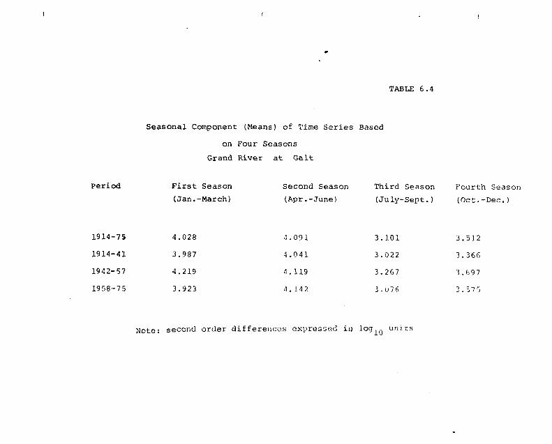
TABLE 6.4

Seasonal Component (Means) of Time Series Based

on Four Seasons

Grand River at Gait

Period

1914-75

1914-41

1942-57

1958-75

First Season

(Jan.-March)

4.028

3.987

4.219

3.923

Second Season

(Apr.-June)

•1.091

4.041

4.119

'). 14 2

Third Season

(July-Sept.)

3.101

3.022

3.267

3.U76

Fourth Season

(Oct.-Dec.)

3.512

3.36S

l.<)97

3.575

Note: second order differences expressed i» log... un.ics

TMrUT SAMPLE f-ERIOr inONlll 'J) -NUrthEK O Yr-St lOOO'J : >%l< h W -

dues

TABLE 6 . 5 . Probability of ExceedanceG.ven Peak Flows in100 Synthetic Samples ofIO.UPO years

'-.LABONAL ME.

JTIi ERRORS

4.02CMG1J 4 .090462 3.100U25 3.51243.')

0 .048135 0.03S345 0 .042751 O.OA02I><-

A 1 0 .17404! 7-TRANEF0F:tt : 0.I7667G STB Cfft : 0.0435003D t 0.-I294D3

* \CRITICAL FLOUS : '

1 2000001. 2 1000001. 3 700000.4 400000. 5 200000. 4 1000C0.7 70000. 8 40000. 9 20000.

10 10000 . 11 7 0 0 0 . 12 4000 .IS 2 0 0 0 . 14 1000 . IS BOO.

LOG CRITICAL FLOWS t147

1013

SET

I

4S

;.

'>1011

1311IS

1710IV2021"

222324252427

J7303132IZ.14'5~'f

z?3<3£7404112IZ414546474019SO

4.301035.402044.345104.000003.30103

MAX FLOW

645577.U02340.745344.-.,47418.4S7234.

<}7l;9OI(.

SiB743l'.'31433.000048.79i960.9?.'*765.

120779.W/3B1.

107173-1.

6"'*til3 '410614.

!21ri4w5.- 435747!

51 :,M6..SCV.07.494215.511071.643200..1725 76.

7MOT4!5V00i*4.51»5:5.."C9178.60197^.743934.V539S22.1OOTS12.77*564.S2i??3.•511771.

U00150.593277.52C714.470054.754742.B34027.056K97•75S--.52.003231.72717C.92593a.

2

81114

1

00000000000000000000

• o ..

. 000000

00c0000000000000000

•o0

60

45433

.00000

.30103

.40204

.84310

.00000

3691215

55432

.84510

.00000

.30103

.4020/.

.9030?

CRITICAL FLOW EXCEEDANCES IN

2

000000000000001•01)

0000

000000

00000000100010000000000

3

0

100010li3200I10001\ J '

000000

0

1001

0221

0010001111

i11

4

2

03454486775

55334489"

634560

S69352311S754921213384564

554564544743704655

sa59514457sa425156536U

•" 4 1

515955

6258

5943607463526257£'3541757725774S335646045636250

6

40739436434B3433703613523713004173393633763S437034t)3633'M7149

" 3 0 2

353333335379340 •354

3623703413713643743C635139137?3553B7367 .347414352416 "379323372379382

7

3178427968067151047792794848824843763025794020B317908297987«2

"B41 "

801007874036307761

796737!34O30481374S811820767870

MS807779810790052760S58301795067G24842

10 THOUSAND YkS

8

219822792127225121S622S6217721432214220O224722382249-•1872224.223321U42197219122S4"2247

220022342292215522232142

220621062224214222102162217522342176231022052S4222432145222922452157224121722150222521792263

9

5124524351445098r,09B527951R951S35123517451445193•MO.!5146521:002715217520851615217VJTM

SI 3851365332520552.415270

"5193

524151105228507951S7SJ07514351V4515452145179511352115131513652975232513552003254 .5214

10

82140237516*50L240145U21501946232

sis:em0172G230U 107B109I1J66

816302048la9(*1S4B223"0222

81733175IM72821501R9022/*

C253« j l914331673222".0123240S2-".60235E212313731 !0e22001788197017632338154C13481658151821A

11

•?1E»91949177913SVlOa91B4.91779191

"120912491049 172914991109181•-.1499120915291U191?!7»'O3

7173712991779169917?9 1.33

71379177914171947|'.'470*j0720071759137-71327137•?1689191920791437160910471607100914991269153

12

93-! 1

982073209B1478129U40

•VJ39V31V9H169B209B2470437U.U'IUZZ7U-J9^057-.I'O

91121

91247

•'B15

'/£;?"*

78.56

7*340

90439S337C31713 -j-i

7S24';'fl25'•3219C169344930473537^43734273289C2090269**41783478217C219033904598419fi2198347830

13

9790?9!,39'UB77C99*<0v97«57*>87

9'?7377909994V7V 1

97V6'IV-14

77£j/'

7VV579U070V 49 W 29/0/

77749V37979177729OVQ

7739

997179917973•vvfl49775

77S7977'j9973?7"299947991990779-V197V0977197389971777099949993

771349971

14

10000100001000010000V77G1000010000?W7

1000010000100001 VOW100001000079 V9IOC/010000•>9-/9

11)0001 IK. '.0101,00

10000100009779

K'0001 C'000

97V3

1000910000

1 ooc-o100)0777 V

100001000010000100001000'.i

100007779

lOO'.'O10000100001000010000999910000l&OOO1000010000

15

.000010000[0»>Ot>

lOOuOIC'V'r-

10'J.IO

lCG'/O

lv'jO"

10000

1 ocoo100"01000010<*.0"

10'JOO

1 o'...>:lv'iW100"01000010000ll'.I'OO

1 vuua

1000010000

100001 0000100CO

10000

ioroo10'jOO

1000010001K-X'O10009100001000010000100001000010000100001000010000100001000010000100001000010000

MIN rLCl

13'./'1304I)v7l.'.fci.

t"**,llv'.Iv6>V -T

J -'.40

L 7i~4

11'- *

; I'! 0lilt.1 4 '}

•>•/1

'. 'J~,*J

\ %2

''}<1 jtiO

11, ! 11":: 1

1 '.-'•'

C'A.5

13-0\.2r)7

3 1 M

1 ,77iZi>'.ir<. 1'.' 1'

10^713671173

121. >

1 ['••!.

I': I.11' »?.ur>.IC77.1233.1457.1)12.

1212.13;'!.I l-j4.1321.

I

III

*) Number shown in the heading of the columns of Main Table, relatethrough this table to the values of critical flows whose number of exce.ces is shown in the Table.

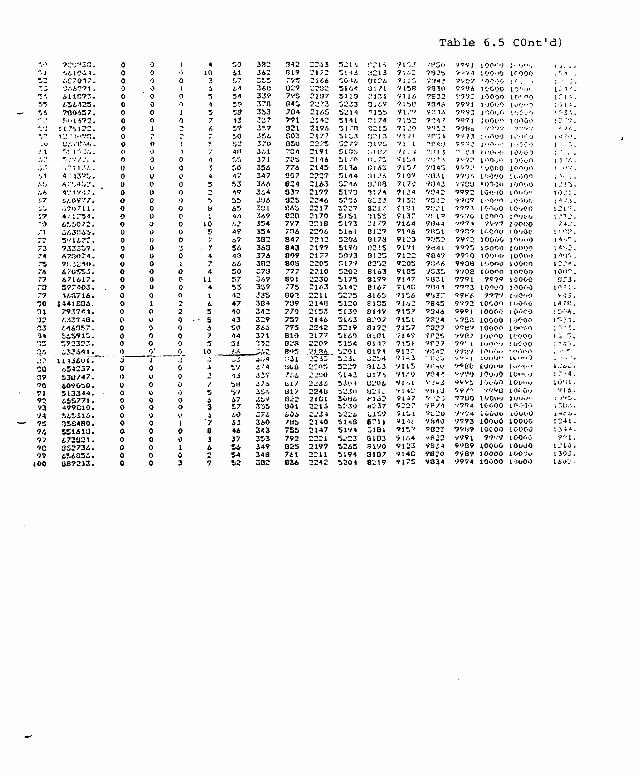
Table 6.5 COnt'd)

'-.' 1

". ZK. -

• • • •

5-i• ' . '

' / '

t , t

! I

-.1

'.7

J'J

57ro/i7773747374777377?0ni3215331•13

j >

CO

70

9?737 A7394777077100

'.A1'.V. 1.

.-.C7017.

A11C77..41442S.700437.'•'•1572.

' 1 7*1122.

I,'.'. /!*•'*',» .

' _ " • • / . ' . ' .

:. '• 1 1 . : . ' . .

1 '1JV"J.

«?iv< 7! 'i/.07'.'7.

.'.?i> 71 1.

4H.-5).4f.iO'I2.•j4J"45.5'.' tA?T.733337.A7:l»74.9!. ;^no.470553.471417.597«03. .140714.

1441CDA.7737*1.•*,;537 4 8 .

v443"<7.345915.372327..

11)3401.

SZU/-17.

&0VO1O.513344.455771.499010.

1SI34B0.3514IU.473U21.352734.454034.0B72J3.

00000000

0000000

0000000000000000000000

0I)0

000000.0000

001)

^>

0000

-,00

00u000000000000000100000ry

100

0000

000000

1

01

00J0

;

000

00<)0000030100002200000

000

000

100103

4

103*,Ti437

-f.

4;

4

5

",'4

s.105?1

474

114I43

• - s47

10._

2/563

"7834

9

3041,7.'.4343053

*?50524ft

y'>

53

55454/1'.»'474734434450575342471043SO4451

J'i37

IS

la•576717

4344373454SI

33234235536HZZ937H353~ ?

354370.5,', 1371334347

344J3A.'.HI3473343343B23433743H2C733A93571SZ3B4342329344371

V.Ii"'4337.l.'A

3Si»

340343353349348302

H421519775027773845704791

S03QSO7!34

7US774307

337325BAS0207V77D4847843809BOS777801775802739770737773BIO023

-3ii'.10B,'L'-4

lil /

317SJ2301

7U5755792025741834

22132172214422322137227321452142"•* 194217?22 75217121142145

2143217722442217217022182204221221772)7722052210223021432211214821532144224221772207

2C0S;: ."JO2~'.Ji

224bL'ICl2214

21*021472221219922112242

5MJ'J0-1&SIM511352335211511151 "TJ

52.'75135i 1 '1SI 143144

3*ffO52043227515151735161520431905073T, 1 7V5202517551420225512051305143S21951405154'-,201

52U7"..143

10U65:?30

5 U S5194•i.-23

S24551945204

J213312681/1"1313147f 155P ! 74

;;:• 13

2l7'j

;.'.t:/

1!. 7?j

BIASaw. A

T. 74012 J321/1155V1 '"73127

017Bi'2153120020231433197B147816SF1C5S811VB207ai72a to 1PI 170171

3143Ul'/i

fij;H-J37

eruOlBlB103B1V031078119

71471 17 15

( 'I"5O: 7325

1 ?G lO7114 7Q32715917713

VI 171"VI .'V" 1 '.V

715

3 904A? 7f! 1.'.» 7'?4 ?

•••r: 1

•>[!<:!

1 -:? 1 3

) •/•; > 1

' VUI",7107 VUJI

7134 VQ-12715•7 iy

713

! 734270.'1

' 71.177144 VIM 47144 711019123 7.'.'S271'712

9«4 1; 9B47

7205 7::'49105 70357147 9BJ.17IIG 7IM1•71 It

11 "J

715715

j 9'JT"

7B45' 7344

7?247157 73277147 7P25715917"71-.

•)l-2 7

' L'j'j

7115 W,u91."

714722

»1 4.715''/1 ti1

) 701 *

• *>2i• 7IV1

7S40; 7B23

•'B229123 t'JH9140 9020917". V334

•)<!<,• j

VV079774T77277717':'?3

""I

7-.-7.1.7'7'J J

• v.i7V-V79r'71l

77!J'.

797277IJ77T7 X

7'iVOV'?7i77"?

7972777577'0990877C-877917T?3

79H6977299OJ

V7SK•^'yyv

7V0?77' 1

v«£ft.

''?V0V J

7780•.•774

99739VIJ7V99197B9frBV9974

10'"" 0100"0: />'*•-•''>

1 '.000100001 JOI.-O

1 'I Of.1"'

J 0001

: "000

1 ,-O"'.>

1O00"1 -.'000I'IOOO

10'j'iO1-'OM<*1 0*^00100109V97l'-COO1000010000100"0I'.-O^'O

100107C7910100777VIOCO"toooo1000010000l'Jl'00I.K....,

JO'J-;O

lOOuOlO'.OO

lOOuO1000097'."?

100001000010000

11" 000; e 'lO'"'"It". 10

',':'•:•'>

10000

!>••>••-j1. .n-: ^

J O'.O?i -.":••-'1

I0.">0«'>

U.001

tooooli'JL'O

10000lO'/OO1000010000iOOOO1000010COO1000010000l'.'O'.Oli.ornj

IOOOO1 oc-oo1 .r..;,,-,

11000: oc-00

twtH- »10'M.J

1 L ^

Iu."/.i'-.

io.;..).-,

1000010000lOOOvIOUOO1007V10000

'..1

1: ''1 ' 1 •••

; " I i

' ' • ' * .

( ^ - . >

! : •

i 3 '/.1 .*•.•

1 ' • ;

}•:>.::

\ 'i •'.',

1 -1 '.

? 4 J .

1 A •,"

I * "v I1

1 ? ?".ion-'a.-j.

1 rt - ; .

•r .j .

14 n*.

1 T- .•*"..

: "• * z.1 j -.,

1 .:«*';.: 1' • -1 .

* ** \'

i"r;.-..

•? •"' 1 .

I.'10.1303-

TABLE 6 . 6

or .IV.;TICAL ri_ou

• AH/I 6 .4 7-1 *'*Z.4 * 1 2 1 3 .

T

0.000 0.000

0.900 0.0000.000 3.000

5T2245.322914 .5256 ( ' 2 .5297=4.5 3 8 7 4 7 .3 4 4 3 1 3 .54961B.35L5J4.5 3 1 6 1 0 .363316 .3 6 5 ? : 5 .569763 .5 7 1 1 3 6 .572J23 .

0.000 0.0000.000 0.0000.000 0.0000.099 ' 0.000

0.0000.0000-9000.0000.000

0.1/00 Q.QK/Q0.000 0.0000.009 0.0000.000 9.000

0.0000.0000.0009. .,000.000

A22313.433641.633946.62S7&7.440614.645577.

0.040 O.OoO0.000 0.0005.000 0.9300.000 0.0000.000 0.000

0.000 0.000

0.000 0.0900.000 0.000

461349. 0.000 0.000

34 A 70353 .5S 471417 .3 * 472S74 .07 4 7 3 8 2 1 .5U 6 7 1 4 5 * .V? 478074 .60 6 6 4 1 0 7 .

U.OCd0.0000.0000.000O.OOO0,0000,000O.GOO

0.000

0.000

o.oco0.0000.0000.0000.000

"00 0.020 0.41-0 3.390 7.609 2l.-14«

000 O.OCO 0 .430 3.3*?0 7 .659 2 1 . *ZH S l . ' ^ S t ' l . 3 « r0^0 O.OZO *>.-»30 3 .410 7 . 6 7 ? 2 l . 4 o f 3 l . l > l m . 3 . ' J •»

000 0.O30 0.44P 3.430 7.49V 21.49'; 51.000 0.9J0 0.-»50 3.430 7.74" 21.529 SI.

° . ? n o ?•>.•?••

.000,000.000,000

ooo000000000000000000.000460

0.0J0 0.470

3.4803.4703.4903.310

iIII

2 1 . 4 1 9 5 1 . 4 0 5 31

0.0300.0300.0300.070

0.400O.-i&O0.4900.490

2.5203.5203.5303.530

7 . C 4 ? 2 1 . 6 4 8 3 ; . 4 2 5 9 1 . 6 1 2 ' l , l | l 9 « . 2 O O ? 9 . 2 ' » 0 79 ,7">o •»•».?«'7 . 0 5 7 2 1 . 4 4 0 5 1 . 4 3 5 a i j . 4 2 2 51.'Ill ' S . T G O •i.B.'-- •*•>.%'.••• " • ? , . - -7 . 9 3 ? 2 1 . 6 5 0 * l . < 3 3 " " d t . d 2 2 ' l . J j : 7 3 , ; < j ' ? ? 9 . 17^ ?7^ 7?.^~ JT , » i -

0.041

0 . 9 4 10 . 0 4O.04i0.04.

0.500 3.540 7.909 21.719 5l.*03 HI.64?0.500O.SOO0.5000.510

3.5503.5503.5503.560

7.91?7.93?7.949

1.7*8 -1.331 31.442 ? ?.•??? '?.7CcI 1 . 7 6 B 5 1 . 3 3 5 6 * . . 4 4 2 9 1 . 4 3 1 > 8 . 2 « v O9.-Jec, 99.?'•»-. f).•».1 1 . 7 6 3 5 1 . 1 6 5 8 1 . 6 6 2 7 l . « l l ^ S . . - * ? 79

0 . 0 4 0 0 . 3 2 0 3 . 5 8 0 7 . 9 5 ? 2 l . i 3 ^ ' J S I . 4 2 0 0 1 . 7 1 2 9 1 . 4 7 1:o 99.yye ?».*»«o »?.'-•••::6b 99.f)»M 71.79O 9'*.9-'-j

77.9V0 ??.?7D

0-01-00.050O.OSO

0.5400.5400.JV>0-tSO

3.00?a.009

1.74Q 11.755 01.7121.9SH 5:.7^i Sl.?52

0.033

0.4300.030

0 . 5 1 0

3.620

3.630

6.007

P. 02'' 2l.VFy 51 .611 M.C02

•1.5i& 3.660O.r-f :• "5.640,

t . ' J l i d l . 0 I 2 9 1 .

i l -'-.Z\<- "«*.."

0.010 O.i.'O

000 0000 0000 0000 0000 0900 0

"oso. 0 3 0. 0 5 00 4 0

. 0 6 0

. 0 4 0

.040

0 . 3 7 0•>.5D000{

c0

.£[19

. 3 8 0•SCfO. 5 8 0. ISO

3333-3

. 660.6110. •00.6*0.690.700

988

.0-7V

.OB?

.09"9.09';

ei

.10?

.L69

SJ.C^B22.01022.09022.09B22. '.Oft22.108?r.i3e

2 1 . ' ' J J31.Wl51.70551.7fll27.001

t-i.tvai.fo&;.'!ot.'H31 .?341.94

»:'/\

: 9;11 71• 91* 91

'.•51 -t.191 *(, ;v i 9(.601 t.611 98. t i l 1/9

'.ilO * '.J30 * *.360 ?9. 1'Ji'j 97.390 99.390 9?.3*0 9?

.Vfv *•*.». 90'J 7 * . fl. *uv '", . ',7'ili 'i'i.'

.9Ct/ 1»,9• Vv'J 79.-)

6 760A"?7O

7 3747374777879

eo8?

75306*.7*4962.755432.773344.789178.793944.

602360.•36027.C39522.

952736.938480.B46891.8*73*0.8C2231.

savsxa!

0.9000.0000.0000.0000.0000.000

o.ooo0.0000.000

0.0000.0000.0000,0000.000

o'.ooo0.000

0.9000.0000.0000.0000.0000.000

0.0000.00(1O.OOJ

0.0000.0000.0000.0000.000

0.0000.000

0.0100.01O0 , 0o.c0 , 00 . 0

0 . 00 . 00 . 0

0 . 00 . 00 . 00 . 00 . 0

0 . 0

0000

0

100

00000

00.010

0.06')O.OdOo.o&o0.0600.9600.&70

0.9700.0700.07O

0.0700.9700.0700.0700.070

O.OQOo.oao

0.5V00.3V00.5900.5900.5900.190

0.6000.6300.6,10

0.4100.4200.4200.4200.420

0.6300.430

3.7603.7603.7402.7603.7A03.780

3,2093.21'/S.239S.23*i.239J.249

3.780 6.2493.730 J.2793.790 f.279

3.7»03./903.8003.0X0 f3.820

3.3203.B3O i

J.269', 2i?.309.309.349

1.359.339

=2.22922.22822.2491'2.21822.28022.206

22.32622.32822.32C

22.33B22.33622.37B22.38U22.406

22.41S22.413

32.073S2.I0S52.13352.13552.13332.1 .1

32.1C352.19S32,223

52*. 24532,25552.27552.29352.283

52.29532.313

92.0i262.Q~~82.07282.10282.11282-112

62.12202.13282.142

92.14262.14282.13202.16262.1C2

•2.21262.222

7 1* !919:9 1

.6Q1

.481• &91.701.701

91.721

9 1?19 1

.741

.761

.761

91.781919 17 191

•5"71

.001

.001

. 9 0 :

.an

.831.dSI

96.400Va.41070.41099.4109B.420VS.420

96-41099.42098.430

98.47.098.43096.44096.440#0.440

78". -30

t*t. 7:0?V.9i->9? .910VV.91099.7109V.910

99.V2099.?2099.920

99.91099.9209 7 . 9 ? •>99.92099.V20

99.73099,930

? y

9 9 .• > 9

9 9 .

??

9 9

9 9 .

99

V 9 .

9 9 .9 V .

9 9 .

9 * .

9 V 0

•ftOV90

7 9 07 9 09 9 0

9 9 09 * 09 9 0

9 9 099-3

9 * 0

v ? . »•>•;9 9 . W Ci". •??••>7* .t'i'j

?9.^Vi

79. fti99.VV0

99"9*C?9.*9CVV.^?<•J9.97Cvv.s-vo

"9**90

V0904B.912181.927I?B.92^938.93U33.•33339.965346.»74743.»B0t>57.

lL143602.L17&123.127409*.1441BI7.

0.0000.0000.0000.0000.9000.0000.0000.0000.0000.0000.0000.000Q.GOO

0.0000.0000.0000.0900.0000.0000.0000.0000.0100.010

a.OKO.OKQ.OV.

0.0100.0200.0200.0290.0200,020

375 32.262 9%.901 99.430 79,930 99.990 9?.990.080 0.630 3.&40 8,419 22.43B 52,403 82.272 91.901 98.450 9^.93-J V9.9«0 9«.?V.;.OHO 0.A40 3.840 8.419 22.460 52.423 J2.292 91.901 93.460 99.930 99.990 «9.9'/0.060 0.640 3.»30 B.429 22.473 52.455 B2.3Q2 91.701 98.470 99.930 99.9V0 99.9'0.030 0.640 3.860 8.429 22.508 52.535 92.312 91.901 98.470 99.930 99.990 V»."J90.090 0.650 3.840 E.449 22.558 52.605 82.322 ?l.V3l *8.460 9?.930 99.990 V9.?'*.J.090 0.650 3.S90 •.469 Z2.6 92.4-tS 32.3J2 91.951 98.490 97.930 99.990

0.020 0.070 0.6600.020 0.090 0.&700.020 0.100 0.680

3.910 8.519 22.72S 52.775 C2.36? 91.971 90.510 *9 .9»0 ?»-9"»f>3.920 8.37» 22.743 52.763 82.392 91 .9« i 99.520 99.940 9«.V90

V.9-»O

0.030 O.tOO 0.700 4.070 8.449 22.S18 52.055 32.512 92.021 98.530 99.930 -79.790 ''?.' '00.020 O.llO 0.710 4.140 a.t&9 22.6S8 52.945 82.532 92.041 V8.340 99.930 99.990 99.9?^0.030 O.llv 0.740 4.160 8.759 22.918 53.035 62-342 92.061 V9.6oO 99.930 9?."90 9?.?10

0.000 0.020 0.030 0.120 0.740 4.190 8.779 23.099 53.315 82.652 92.261 'O.733 79.970 99.V9C 99.V*'.-

I

TABLE 6.7

Estimates of Maximum Mean Daily Flows with .10,000 year Return Period Using

Frequency curves

Grand River at Gait

{Flow in cfs)

Period ofrecord used

1914-41

1942-57

1958-75

1914-75

Values based onrecorded parameters

Values based on the upper9 5% confidence limit of there cordedpar ante ters

Assuming log-normal Assuming log-Pearson Assuming log-normal Assuming log-distribution type III distribution distribution Pearson type III

distribution

50,300

98,500

126,800

87,600

46,900

95,900

67,700

67,700

75,169

198,800

326,000

128,000

148,662

832,000

826,000

180,000

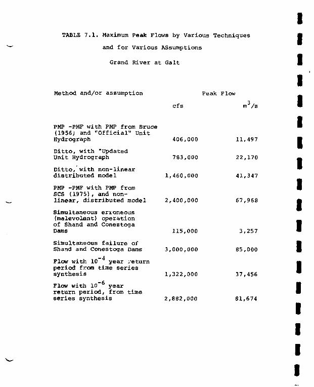
TABLE 7.1. Maximum Peak Flows by Various

and for Various Assumptions

Grand River at Gait

Method and/or assumption

PMP -PMF with PMP from Bruce(1956) and "Official" UnitHydrograph

Ditto, with "UpdatedUnit Hydrograph

Ditto, with non-lineardistributed model

PMP -PMF with PMP fromSCS (1975), and non-linear, distributed model

Simultaneous erroneous(malevolent) operationof Shand and ConestogaDams

Simultaneous failure ofShand and Conestoga Dams

Flow with 10~ year returnperiod from time seriessynthesis

Flow with 10 yearreturn period, from timeseries synthesis

Techniques

Peak Flow

cfs

406,000

783,000

1,460,000

2,400,000

115,000

3,000,000

1,322,000

2,882,000

m3/s

11,497

22,170

41,347

67,968

3,257

85,000

37,456

81,674

111111111111111111

FIGURES

A \Lulh

ys

(p.

(*>

\

1?\BelwoodJ w —

lake / ^

Everton Reservoir

• ^ f Bode,., port

Figure 2.0. Limits of the Study Basin, Prand River at Gait.

*

•>

*

T

•

* - -

—

>

* - *

5>

—

1

*-*•s

a

>

1PREl

PR08AOVf

_

1 1IMINARY ESTIMAT•LE MAXIMUM PRER SOUTHERN ONT— TROPICAL ST— THUNDERSTOfl

s

s \\

s

V

•>•

ES OFCIPITATIONARIOORMJMS

« | H

»tMR

I4HR

1ft M

it nil

• MR

• HR

• I * IN SMMMIC MILK

Figure 2.1. PMP estimates according to Bruce (1956).

I pr»t!»it«ii«n (i*ch«t} «ait of ih« lOS* m«rldinn lor an WM »f 10 m«fr« «il*l on* 4 hovft' d^rghon711 0-244VA, III-&-2754, M1-D-J7J5.

J j^ ' Depih dreo 4urol«on imto

•* opplird 'o 10 «quor« milli. 6 hovr jtrsbnbl«

Figure 2.2. PMP estimates accordii^to Soil Conservation Service (1975)

f

;

:

i ;

•

i

: ,

! 1

-

. :

1

! i i

; | j

;.: i. . i

I i i

i : j .

*»••

; j |

: . i i; ! 1

! ' " • ' •

1 ' • i

i !. 'i

.'. 1 !

1 ! !

•i '-

: . i

• i :

: i : •

; ' i

• ! : i

, . !

! : i '

! ! <

'•• ! :

* - "

; '

;

- j

i

:

: ' j

'•

— —

i l l

i ' 1.

' ' 1

! hr I• :- i

——-L,

•\i\i ' j

i !i• t i l

'•

• • • i

"-

• ^

1 i •; i*.' : X ; -

: i i:A (

t ; i

. ' '. !

'

• : •

: 1 :

1., . !

: ....

•1 ; :

• !

j i i ;

\-'y. . i

' ' • :

: ' • ' • .

' • '• i : • ! •

/ .

t

• / :

. / : . .

; ' :

!. i : !'.'•.::

•

: i . ;

. . . .

i ;. . . .

1 : •: :

;\i\!

•: T

ime,

h

ou

rs.6

0.:.

: •.

.,:.

...

72 .

. ; .

. .:

r

- ;- Sg-r

• 1 • i -

tr\

! ' • • ' !

ji T( 1 • • ' i

•T .... j 1:- - ' — * * :

J . ; i ;

X^

> • .

ot-i

o

•eo

o,—I

I

sjo jo spuesnoq^ UT

13

3

2-58

woof T9-S0'

Figure 2.4a.Estimation of isohyets of storm of May 16-17, 1974,according to Atmospheric Environment Services.

IIIIIIII

MAP OF

Figure 2.4b.Estimation of isohyets of storm of May 16-17, 1974,according to Ontario Ministry of Natural Resources.

P5K

V !

Boundary ofGrand RiverBasin

UH0352

K H I h / H R 0 - L V l 0 . 0 4 " I V2 0 . 1 " LV3 0 . E " LV4+

P5K

Boundary oGrand RiverBasin

UH

LEGEND

• CALCULATED PEAK FLOWS, TRIANGULAR HYDROGRAPH METHOD• PROBABLE MAXIMUM TORONTO• HAZEL TORONTO (CENTERED)0 MAY 16 - 18 1974• H HUMBER RIVER• HW HUMBER RIVER WESTA SHAND SPILLWAY CAPACITY AT 1395 6 EL.A PROBABLE MAXIMUM CONESTOGO DAM U P BRUCE)

i C.A s= 1,358 SO. Ml.

fOR R$GIONA,L STOjRMI

24 36 46 60 72

TIME IN HOURS

84 96 108 12

Figure 2.6. TYPICAL HYDROGRAPH FOR GALTRun-off Curve N2 85

GRAND RIVERFLOOD INQUIRY

MAY 1974PhlllpiPlannin

STRIP NO

2 4

2 3

2 2

:n

2 0

19

1 8

17

1 6

15

1.4

13

:L2

11

:i 0

9

B

7

6

5

4

3

2

1

FLOW

. 1

0

0

0

0

0

0

0

0

0

0

0

0

0

0

0

0

0

0

0

0

0

0

0

1

DIRECTION

0

0

0

0

0

0

0

0

0

0

0

0

3

2

1

0

0

0

0

0

c0

0

0

0

0

0

0

0

0

0

0

0

0

3

3

3

3

2

1

0

0

0

0

0

0

0

0

0

0

0

0

0

0

0

0

3

2

2

3

4

4

3

2

2

0

0

0

0

0

0

0

0

0

0

0

0

0

0

3

4

3

3

3

3

2

3

3

3

2

3

2

0

2

0

0

0

0

0

0

0

0

3

3

3

4

3

3

2

2

2

3

4

3

2

3

2

2

0

0

0

0

0

0

0

0

4

3

4

4

2

3

2

2

« • >

2

3

2

3

2

3

0

0

0

0

0

0

3

2

to

2

3

Z

3

3

."5

3

3

2

3

4

3

2

2

0

0

0

3

3

V

3

-

\

2

3

4

4

4

4

3

2

4

2

*

3

3

2

1

0

0

0

• " •

3

4

4

,./

3

3

3

3

4

2

3

.'•5

3

4

3

A

4

2

2

1

2

0

0

o

0

0

3

3

4

4

4

2

3

3

4

4

4

3

4

3

3

3

3

2

v-i

0

0

0

0

0

0

0

"7

3

3

3

4

•5

4

3

3

3

3

3

2

0

0

0

0

o

0

0

1

0

0

0

0

4

3

4

0

0

0

0

0

0

0

0

0

0

0

0

0

0

0

0

( . •

0

0

0

0

0

0

0

0

0

0

0

0

0

0

0

0

0

0

•>:,

' * • >

. ; :

?0

1 ' . •

1!'.

\ :••

1-6

I S

14

1.-

j . ••.!

i i .

10

9

H

7

«•

S

4

S

2

1

Figure 2.7a. Example of data contained in the grid square system fordistributed model of Grand River: direction of flow:1 = North; 2 = East; 3 = South; 4 = West).

*****

'.'•Tftjp HO.

2 4

23

2 2

21

20

19

1 0

17

16

15

.1.4

13

1 2

11

10

9

8

7

6

C*

4

3

2

1

I..1-VI-

I

0

n

0

0

0

0

0

o

0

0

0

0

0

0

0

0

0

0

0

0

0

0

0

1

1.:

0

0

0

0

0

0

0

o

0

0

0

0

20

IV

20

0

0

0

0

0

0

0

0

0

0

0

0

0

0

0

0

o

0

0

21

20

19

18

17

18

0

0

0

0

0

0

0

0

0

0

0

0

0

0

0

o

24

23

"> o

21

20

1'?

16

15

14

0

0

0

0

0

0

0

0

0

0

0

0

0

0

•v

25

21

20

IV

18

15

14

13

12

13

12

0

10

0

0

0

r,

0

0

0

0

26

25

24

23

20

19

18

17

16

15

14

11

10

11

10

9

0

0

0

0

0

0

0

0

27

•"><•'•

25

24

IV

18

17

16

15

14

13

12

9

8

9

8

0

0

0

0

0

0

:> a

27

28

25

22

1°

J.R

17

16

15

14

13

12

11

10

7

6

7

0

0

0

.<0

2?

28

2 7

26

27

24

21

20

19

IB

17

IB

17

14

11

12

7

6

5

6

0

0

>•»

..' 1

30

29

28

25

24

-'\

22

21

20

21

18

17

16

15

10

9

a

5

4

5

4

0

0

< •

n

0

2 7

26

25

24

23

24

21

?.O

19

18

17

12

11

6

5

4

3

r-o

3

0

0

n

(i

•:..

0

0

Q

o

0

23

22

21

20

19

14

13

6

.j

4

3

r-i

1

0

0

n

0

0

0

• • • >

0

0

o

0

0

2 3

2 2

21

0

0

0

0

0

0

0

0

0

0

0

o

( - •

0

0

o

0

0

0

0

0

0

0

0

0

0

0

0

0

0

0

0

;.' i

' Q

I f>

l:i

I1.:

1:.',

1 2

11

!. 0

r''

8

/

6

4

3

2

1

Figure 2.7b. Example of data contained in the grid system fordistricted model of Grand River: Order of routingof rur-... f (squares with largest numbers are consideredfirst).

SI KIP NO.

2 4

:?3

1'* 2

21

20

19

18

17

16

15

14

13

12

11

10

9

8

7

6

5

4

3

2

1

t OF

1

0

(i

0

0

0

0

0

0

0

0

0'

0

0

0

0

0

0

0

0

0

0

0

0

1

GRID

0

n

0

0

0

0

0

0

0

0

0

0

0

':>

0

0

0

0

0

0

0

0

0

0

0

0

0

0

0

0

0

0

0

0

0

1

4

9

11

0

0

0

0

0

0

0

0

0

0

0

0

0

0

0

0

0

3

0

0

1

0

12

13

0

0

0

0

0

0

0

0

0

0

0

0

0

0

0

0

1

12

14

15

16

17

0

15

19

20

0

1

0

0

0

0

0

0

0

0

0

0

1

2

5

7

0

1

i"iiL.

18

0

0

1

21

22

2

3

1

0

0

0

0

0

0

0

0

0

0

1

0

0

0

4

19

1

0

0

1

28

29

4

7

0

0

0

0

0

0

0

1

0

0

0

3

32

34

41

62

65

89

90

3

4

30

31

8

0

0

0

1

5

7

12

1

1

1

2

26

0

0

0

1

21

91

0

99

100

143

9

0

0

0

0

1

0

13

17

21

23

24

25

0

4

15

19

20

96

97

98

0

145

0

0

0

0

(I

0

o

0

1

0

0

0

0

'"<

3

9

0

-;,

0

l

3

150

153

1

0

0

0

l)

0

0

0

0

0

0

1

3

4

7

8

0

1

0

1

2

3

4

159

0

0

••

(•

0

0

0

0

0

0

0

0

0

0

1

0

0

0

0

0

0

0

0

160

0

0

•J

< • '

0

0

0

0

o

0

0

0

0

0

0

0

0

0

0

0

0

0

0

0

0

i1 1

20

| V

!B

17

16

13

14

\A

12

:l .1

10

9

8

7

6

5

4

3

2

1

Figure 2.7c. Example of data contained in the grid system for .distributed model of Grand River: Number of grid <•squares drained by each square.

1

!

i

I

• i

i j

0)

o— * ) —

o

,ds

; 3

! gp

f

i

—

•an

25

20

15

1 !

i

j

1 ! 1

- •

—

y

-

—

-

/

—

\ \ 6 12.

—

Figure

i i

'• :

4

... .

i

-

• • -

• - -

/

—

—

/

' ' i

, :

• :

\ ' '

• ,• T ~ - - '

r--

—

r

—18 24 ' 30 3(

71-

-TimeI

!

" The """Of f i

|

•

iT ho;

exal1

I i I

i !

i

...

\

....

—

Timeh

0

6

12

18

24

30

36

42

48

54

60

66

72

Flowcfs

0

cnooL2000

L8000

!4000

>1000

L8000

L5000

.2000

9000

6000

3000

0

-

-

—

-

i 1

1 '•

i ! '

--

>-

11

5_ . _42.._. 48_. 54 60 -66. -.7;

irs"" • " •

I;

• ^ :

: : ; ;

6 hour Uniti |

;

jt jl ,

Hydrograph

- : !

Flow, thousands of cfs

H(D

aH-f t

toa

SH01

•a3"

fu

f t

c3a>01ft0nn

SB

aH0

h(

VIc•a i

3*

aoH co

JTHl

2 °r f O0 ^

3 M-O 0Hi 0)Mi ftH- H-0 0H - 3BlM O

: Mi

1-3 VC

3m

3"0c

o

Average precipitationin river basin, inches per 6 h.

2

rt

0>t3

I

11

s1

H9

H-3

0.25

o.50

0.75I

! 21 0 3 . 6 9 h

. 16 May 17, 1980

: a • ;

Note: Precipitation recorded_ ... at xracrorfi is indicative but

not representative of, precipitation in the river ba.

• Figur<j 4.3. Hydrograph separation for derivation of "Updated

> t> nouriun.it Hydrograph ;

j-j-7-| -r-^-j— --:-r-hyetograph; b j -Grand River~af Gait hydrograph

! , : I • • •

TT

Time

h

0

6

12

18

24

30

36

4?48

*,d

.60

Flow

cfs

•• 0

1580

2167,0

5 9 n 0 0

26000

14J0p

9060

610Q

3740

1450

0

~T

6 12 18 24 30 36

Figu re ; 4 ; 4- "Updated" 6 hour Unit Jlydrographi

. 4.2 4|8 . 5.4 . 6|0 h.Ti

Note: For PMP hyetograph see Figure 4.2

72 96

Time in hours

Figure 4.5. Hydrograph of PMF resulting from applicationof a thunderstorm PMP + h PMP to "updated"Unit Hydrograph.

O O O O O C O O C ' 9 0 ' 7 9 0 9 0 0 0 I

Measured

Generatedby model/**

Figure 4 . h . Cr.ind !>i"e.- c\i.Gait. Calibration of nor.-Ji:distributed model(Flood of May 17-1?,1930)

III

1I

¥t X

XX T- XXX XX^XX

XXX *

Measured flow, cfs

Estimated flow, cfs

Time , hours (Time originrmidnight of May 14,197 4)

C • r* r\

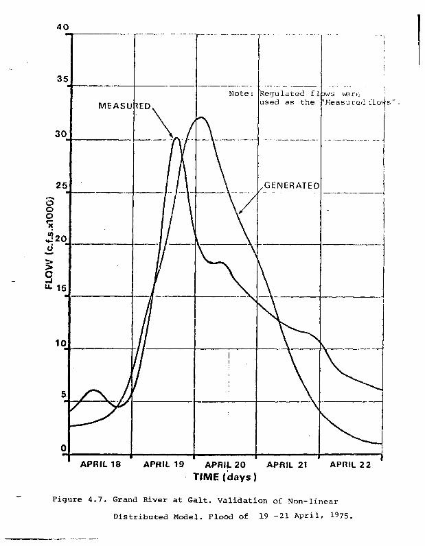
Regulatedused as the

APRIL 18 APRIL 19 APRIL 20 APRIL 21

TIME (days)APRIL 22

Figure 4.7. Grand River at Gait. Validation of Non-linear

Distributed Model. Flood of 19 -21 April, 1975.

1,600

12 24 36 ^8 60

Fzgure [4.8. Probable Max$n iDistribiite|d

II1IIII1

mMJ

KCTiOM THMOUOH

•tenon «-«

Figure 5.1

SHANO CAM - PROJECT ARRANGEMENTOH»ND RIVER COHSCRWTION COMMISSION

S o u r c e : rt 6 ACRE3 a COMPANY LIMITE

SECTION > - B

F i g u r e CONESTOGO DAM - PROJECT ARRANGEMENT5 ^ 2 < iR*ND R I V E B CONSERV»T:OS COMMISSION

Source: C i L C a CC' - ' " ' - ' - 1 - " ^ - V ' _ k

0L1.01 1.1 13 1.5 2 3 4 567 10 20 30 50 70 100

RECURRENCE INTERVAL IN YEARSFigure 5.3. 'eak flow versus recurrence interv.il, Grind river .it "".i , I') '. '•.-

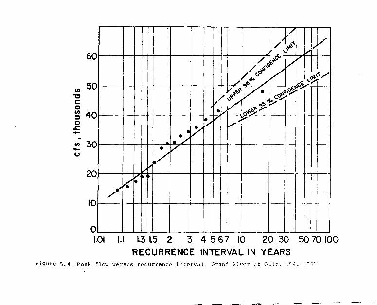
Cfl•ocoCO

60

50

40

•

/

s

t \

1

X 1

42 30o

20

10

1.01 I.I 13 1.5 2 3 4 567 10 20 30 50 70 100RECURRENCE INTERVAL IN YEARS

Figure 5.4. Peak flow versus recurrence interval, (Vrnnd River nt Cilt, ;.Q-i -1 ° '>"•'

to•ocoao

JZ

60

50

40

30

y

/

Jt

/

A*i%

/4

* 20u

10

01-01 1.1 1.3 1.5 2 3 4 5 6 7 10 20 30 50 70 100

RECURRENCE INTERVAL IN YEARSFigure 5.5. Peak flow versus recurrence interval, Grand River at Gait, 195B- 1975.

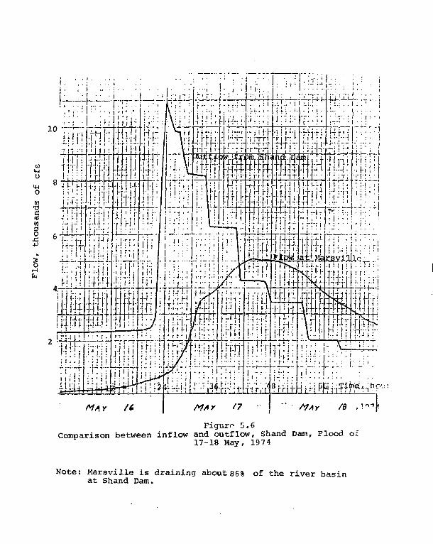
01iwO

t-iO

in'O

to30si

Figure 5.6Comparison between inflow and outflow, Shand Dam, Flood o£

17-18 May, 1974

Note: Marsville is draining about 86% of the river basinat Shand Dam.

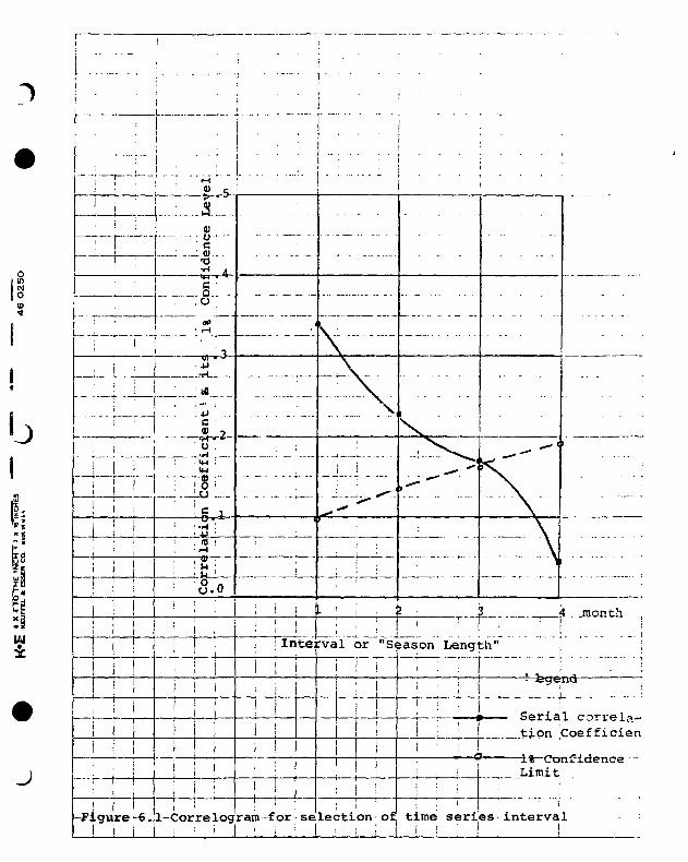
1

1

1

:—

i|i

i"!|1

j1

i

I1

•

— - —

1

• - T -

1

J

1|

|ii

1

!

ij

! i '-Figure -6.

1 i i

- — ; - •

_

:

!

,

j

-iL-5-.fl.._-

au—

•a

o, o

up

_ d

c •

o ...-H

"8T-

S i•H :*i '

u I

5.o

i

i iii

i

ii

1-Cor

iii

i

ii

re logi

— - •

— . —

— - ' — -

- • •

v—-—~—i —

—

! j I JL !

' i l l '

i :Interval1 !

1 j

I ii !1 !

• i

ram -for s e

i

I

. . . ... ._.

\

_ . \i

? : 3i ! ' : 1 • :

~ • • - •

t. .month ,

or "Season Length" ,

i

1

i

ii j

I ii !

lection-o£! I I

t :

- egena: i

1 ' j tion1

; i

Line seri

1 * 1_U

Limit

es interva

1 correln-Coefficien

nfidence•-

1 ;

0»

. ' . . •

8 iliiisss* s— inrotM _ m

°§§§§8o

oo

PROBABILITY OF EXCEEDANCE ,%

160 —

M-l

o01Tf(0(0

|

c•r-l

w3o

sA)4Jcn

•rH

Dg

•H

(0

50-

40-

\Average relationship

Conservative relat io

i6R

Legend

1930 - 19411942 - 1957

A 1958 - 1978

50

Maximum mean daily flow, inthousands of cfs

Figure 6.3. Relationship between mean daily and instantaneous

annual maximum flows, Grand River at Gait.

50- <s OBSERVED- COMPUTED

15200

Figure

300 400 500 600 700 800 900 1000 1100G - D i s c h o r g e d O O O c f s ) -

. 1 S t a g e - D i s cho r r j e R e l a t i o n f o r M i s s i s s i p p i R i v e r , T a r h e r t L c n d i n j

7

© OBSERVED- COMPUTED

15.200 300 400 500 600 700 800

Q - D i s c h a r g e ! 1 0 0 0 c f s ) -» -

F i g u r e 3 . 2 S t a g e - D i s c h a r g e R e l a t i o n f o r . V i ; : , - ; . . •..: hV i

900 1000 1100

' ? r : L i i :• •-! : ' . v ! . L a .

89

880 -

870 -

860 -

UJ 8 5 0 -

UJ

840 -

830-

820

\

Note- End of recorded profile —•|

\

\

Y

\ — — _

LEGEND '

Profile from HEC-2Profile from Graphical TechniqueRecorded ProfileChannel InvertBridge Location

Figure 8. 3. Comparison betv/eenrecorded and calculated water profilesat Gait, for the flay 197 4peak floodflov/.

\

\

\

Hill, Hi . in in iCross-section Locations

T l I I | I L_T_LJ I \ I l I.in

10 14 16 18 20 22

MAX. LEVEL

MAX. FLOW

INCREASING FLOOD

AVERAGECURVE

.(a)natic re

100 150Q(m 3 /S)

Figure 8.5. Schematic representation of staqe

discharge relationship during a flood event

0(flow)

t (time)

(b)Figure 8.4. Level variation in time during a flood c.ver.i

Figure 8.6. Water profile along a river reach during

a flood event

APPENDICES

APPENDIX 1

LETTER FROM CANADIAN CLIMATE CENTRE (AES)

DATED NOVEMBER 16, 1979

AJ ,

: f"iivironrTiont f.nvirunncntcru utmosphdriqui??*'• f ishnrii s itiui kMvirwnniew C<in<><J/} Prchcs i't Knvimnnemrnt" Alfiios

Canadian Climate Centre4905 Duffprin StreetDownsview, OntarioM3I1 5T4

November If., 19798957-1

Prof. S.l. SolomonCivil Engineering Dept.University of WaterlooWaterloo, Ontario

Dear Professor Solomon:

Reference is to our phone conservation (Solomoii/ilogg) ofNovember 8, 1979, concerning probable maximum precipitation analysisof the Grand River Basin. As discussed at that time, the study byJ.P. Bruce entitled, "Preliminary Estimates of Probable MaximumPrecipitation Over Southern Ontario" is the only relevant study ofwhich I am aware. A copy is enclosed.

If it is decided that a more detailed analysis is requiredby Lhe Atomic Energy Control Board and AES agrees to participate, atime frame of our months seems reasonable. It should be noted, howeverthat the time of the personnel who would be involved is alreadyheavily committed for the period February through May, 1980. The pro-posed study would consist of the following:

i) Collection of available meteorological dataii) Historical storm analysesiii) Maximum atmospheric moisture analysisiv) Storm maximizationv) Statistical analysis (Hershfield)

In addition, depending on your requirements, it may be necessary tocomplete:

vi) Estimation rt maximum snow accumulationvii) Determination of upper limits to maximum temperature

sequences for snowmelt purposesviii) Seasonal reduction of PMP estimate for rain on snow

event maximization

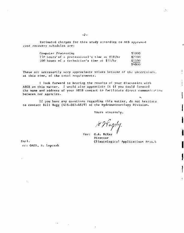
- 2 -

Estimated charges for this study according to AES approved

cost recovery schedules are:

Computer Processing $1000150 hours'of a professional's time at $18/hr $?700100 hours of :t technician's time at $ll/hr $1 100

$4800

These are necessarily very approximate values because of the? uncertainty,at this time, of the total requirements.

I look forward to hearing the results of your discussion withAECB on this matter. I would also appreciate it if you could forwardthe name and address of your AECB contact to facilitate direct communic.i! ionbetween our agencies.

If you have any questions regarding this matter, do not hesitateto contact Bill Hogg (416-667-4619) of the Hydrometeorolopy Division.

Yours sincerely,

for: C.A. McKayDirector

E n d . Cl tm.-itological Applicationscc: OAES, S. Lapczak

, APPENDIX 2

Non-linear Distributed Rainfall-Runoff Model

Part I: Model Description

Part II:M6del Code

VOL. 13. NO. 3APPENDIX 3., PART I: MODEL DESCRIPTION

WATER RESOURCES R1.SEARCH J I M

Distributed Numerical Model for llstimaling Runoff andSediment Discharge of Ungaged Rivers

1. The Information System

S. K. C U T i A

Dt'parlnn'tlt of Cicif tJixiHtTWi}!. \ttditl C micrulv. \tiwtrt'tU. (/HC/IIV. Camilla

S. I. SOLOMON

Department oj Civil Engineering. University oj H'alerloo. Waterloo, Ontario. Canada

INTRODUCTION

This is the first of a series of three papers describing adistributed hydrologic model which has been applied in vari-ous areas of Ontario for estimation of runoff and sedimentyield al any point of a river basin. The model is capable ofsynthesizing ihe hydrology of the basin under current andmodified conditions. In order that it can be easily applied tomost areas, the model is designed to take as input those datawhich are usually available for most ureas. Also, the mathe-matical relationships used for simulating various hydrologicand sediment erosion-transportation processes are thosewhich can bo applied with the available data. Such a selection,at limes, has led to adaptation of a relationship which is moreempirical in comparison to another one which may describebelter the physics of the phenomenon but needs use of datawhich are usually not available. Inputs to the models areprecipitation and temperature data, in addition to data on thetopography, river network, and land use and land cover, soil,and geologic characteristics. Measured flow and sediment dis-charge data are required for calibration and validation tests,although the model gives reasonably good results with param-eters estimated in neighboring river basins. The first paperdescribes the information system for setting up the model, thesecond is devoted to the description oi the runoffand sedimentmodel, and the third analyses in detail the results of the modelas compared with other more conventional techniques anddiscusses work in progress to extend its use to the analysis ofseveral water resources problems.

THE NEED FOR A DISTRIBUTED MODEL

in a recent review of hydrologic models, Jackson [1975]makes an interesting distinction between two categories ofsuch models. She divides them into descriptive and pre-scriptive hydrologic models. According to her a descriptivemodel is one that describes some process or system, hopefullyproviding added insights into the actual operation of the sys-tem, A prescriptive model, on the other hand, is one intendedfor planning use because it instructs the analyst on how toextract ihe best results from a system. The authors doubt thata hydroiogic model can be prescriptive without being descrip-tive. Without describing the process and obtaining insight into

Copyright © 1977 by ihe American Geophysical Union.

I'jper number 7W0I90. 6M

the functioning of the system ii is impossible to apply ii forextracting the best results from it for the simple reason tha: theusual interference with the system in putting it to some useresults in the modification of the system, in changes of its basiccharacteristics and. consequently. o( its output. The myth thaia model which reproduces best the statistical characteristics ofthe recorded time scries is a iiood prescriptive (and. 1'OT sonic.good descriptive) model is so enshrined in the mmJs ol *»•::•,«;hydrologists. the simple fact that the river basin after deielop-ment is a different basin titan it «as before development nfrequently ignored. That this may be al least partly the cau<cof faulty design and operation should not suiprise us.

Figure 1 illustrates the effect of changes in characteristic ofa river basin due to a forest fire on the corresponding fi.v.vhydrograph. Whereas such significant changes cannot e-c.:r>ethe attention of the slalistician-hydrologist. more .-.jbtle h.-drologic changes due lo gradual modification c! the river b.i>ir.characteristics arc frequently ignored or. .a .he mo*;, men-tioned as a problem. Solotnun [19751 ?-.ves another *'.rikir£example from many others available of a change in the h>dro-logic regime of a river as a result of mans imer'crcrice »::ri.:.

It is also not surprising that real descriptive models ('scrr.:deterministic" models), which at least make a valiant attemptto describe the hydrologic processes and provide insight iir.othe functioning of the system, were nol even mentioned inJackson's discussion. For the purpose of this paper, 'parame-tric' or semidelerminisiic hydrologic models are defined asmodels which are based on physical analysis of the hydrologicprocesses but which contain a number of parameters(coefficients) which arc obtained empirically or statistically,exogenously or endogenously, i.e.. in ;he process oi'calibratingthe model. A similar approach was adopted by .Vviv [l')('7] indeveloping a sediment model. In the opinion of the .minors,such models, however weak they may be at this »uac. repre-sent, nevertheless, the best hope of obtaining desenptive-pre-scriptive models. One day. probably not too far away. >uchmodels will become lools able lo describe lire system, its func-tioning, and the effects of changes brought about by develop-ment in ihe system and its outputs (occasionally also its :i-puls) and thus become a real aid in testing the elVec.s o:'various alternatives.

The major problems related to the development ,md appli-cation of scmidetern^nislic models have been so ur lire lack iv.'

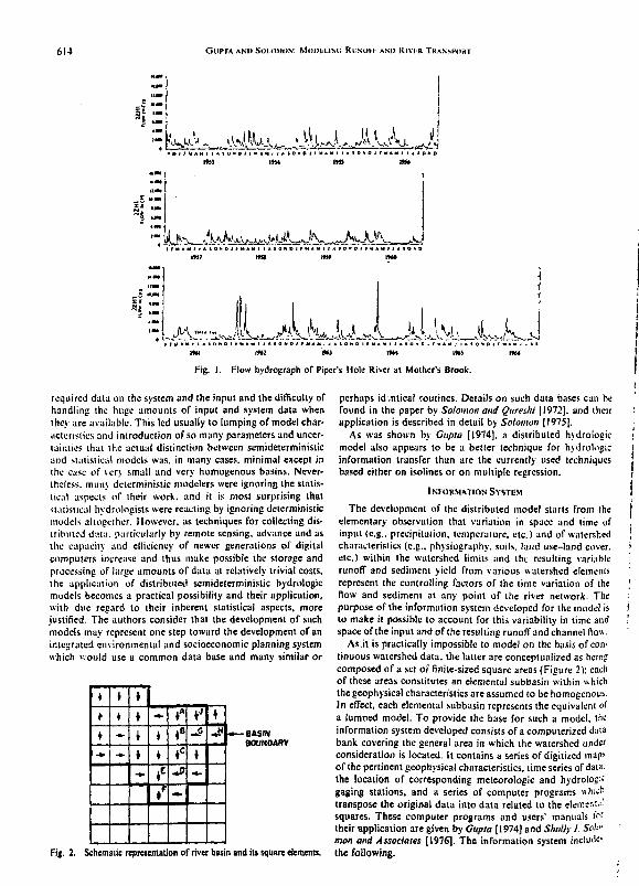
614 GUPTA ANIJSOIOMON: Mum:i-iNi; RI:NUH AMI RIVI-R TRANSPORT

Sf —

*.m

IHI IH2 IHJ »H IHi

Fig. 1. Flow hydrograph of Piper's Hole River al Mother's Brook.

required data on the system and the input and the difficulty ofhandling the huge amounts of input and system data whenthey are available. This led usually to lumping of model char-acteristics and introduction of so many parameters and uncer-tainties that the actual distinction between semideterminislicand statistical models was, in many cases, minimal except inthe case of v m small and very homogenous basins. Never-theless, many deterministic modelers were ignoring the statis-tical aspects of their work, and it is most surprising thatstatistical hydrologists were reacting by ignoring deterministicmodels altogether. However, as techniques for collecting dis-tributed data, particularly by remote sensing, advance and asthe capacity and efficiency of newer generations of digitalcomputers increase and thus make possible the storage andprocessing of large amounts of data at relatively trivial costs,the application of distributed scmideterministic hydrologicmodels becomes a practical possibility and their application,with due regard to their inherent statistical aspects, morejustified. The authors consider thai the development of suchmodels may represent one step toward the development of anintegrated environmental and socioeconomic planning systemwhich >vould use a common data base and many similar or

-BASINBOUNDARY

•

i- -

•tt•-

iTi

u

•A

•8

•c

-

Fig. 2. Schematic representation of river basin and its square elements.

perhaps identical routines. Details on such data bases can hefound in the paper by Solomon and Qureshi [1972]. and theirapplication is described in detail by Solomon [I975J.

As was shown by Gupta J1974], a distributed hydrologicmodel also appears to be a better technique for h\<lrologicinformation transfer than are the currently used techniquesbased either on isolines or on multiple regression.

INFORMATION SYSTEM

The development of the distributed model starts from theelementary observation that variation in space and time ofinput (e.g.. precipitation, temperature, etc.) and of watershedcharacteristics (e.g., physiography, soils, land use-land cover,etc.) within the watershed limits and iht resulting variablerunoff and sediment yield from various watershed elementsrepresent the controlling factors of the lime variation of theflow and sediment at any point of the river network. Thepurpose of the information system developed for the model isto make it possible to account for this variability in time andspace of the input and of the resulting runoff and channel fio».

As.il is practically impossible to model on the basis of con-tinuous watershed data, the latter are conceptualized as beingcomposed of a set of finite-sized square areas (Figure 2): eachof these areas constitutes an elemental subbasin within whichthe geophysical characteristics are assumed to be homogenousIn effect, each elemental subbasin represents the equivalent ofa lumoed model. To provide the base for such a model, ihcinformation system developed consists of a computerized databank covering the general area in which the watershed underconsideration is located. It contains a series of digitized map*of the pertinent geophysical characteristics, lime series of data,the location of corresponding meteorologic and hydrologygaging stations, and a series of computer programs ntiai'-transpose the original data into data related to the element-squares. These computer programs and users' manuals K'their application are given by Gwp/a [1974] and $/«///>•/. Soli-mon and Associates [1976]. The information system includethe following.

GuTTA AN[J StU.OMOH: MolU : l INli RL.NO11 ; AND RlYl R T K A N S T O K T 61.S

b) INOICESOF RE-

LATIVE LAND USE

EFFECTS ON FLOW

5EOMENT

ol OERIVEO SOIL

(TOPERTIES FOB

MAW SOIL FAMILIES

IN THE WATERSHED

HYDROMORPHOLO-

GICAL DATA S

lELATIOtl SNIPS

I I T I A L ESTIMATESV (MODEL

PARAMETERS

I HOURLYUDAILY

AMD

Y SEDIU-

« I GUAM

Fig. 3. Input-output of the model.

Geophysical data. These are data consisting of the distrib-uted information on topography, soils, surflcial geology, andland use-land cover. This information is derived by (I) digi-tizing the topographic maps along the contours and, in turn,determining the topographic characteristics of each grid ele-ment by computer by using appropriate programs, (2) digi-tizing the boundaries of different soils, surficial rack types, andland use-land cover polygons marked on the soil and land usemaps of the area and determining the percentages of each soiland land use-land cover type in each grid element by using thecomputer programs developed for this purpose, and (3) stor-ing well log data and suil and geological analysis data availablein the area; determining relationships between these data andtype of soil, surficial formations, and land use-land cover; andderiving from these various indices regarding infiltration, per-colation, field capacity, and erodibility for each elementalsquare. The topographic information is stored in the basin file,and the pedologic and land use-land cover data are stored inthe soils and land use file (Figure 3).

Drainage system characteristics. ( I ) T h e number and

length of the river channels of each order in the channel systemin the area under consideration are included in drainage sys-tem characteristics. This ordering system is the same as thatdefined by Slrahler [1964]. (2) The orders of the channelsfeeding and draining each grid element are also included. Thisinformation is derived from the drainage maps and supple-mented by the aerial photographs of the area. For large basinsthe information is obtained in a regionalized manner. (3)Drainage characteristics also include hydromorphological(river channel regime) relationships between river flow, on onehand, and channel width, depth, area, and velocity on theother. Separate relationships are used for the main channeland flood plain. These relationships are obtained by statisticalanalysis of the data from flow measurements. The drainagesystem characteristics are stored in the hydromorphologicalfile.

Measurements of flow nnd sediment load. These measure-ments, made at the hydrometric stations in the area, are storedin the hydrological data file. The (low measurement data in-

clude, in addition to data on stage, flow, and sediment. d:u.i or.cross-sectional area. Ai'dth. aierage depth, and ieloc;:>.Where they are available, data on sediment gr.iin size d:siri'r._-tion are also included. Data on flow width, average dcp'.h. J.rivelocity are used to develop the i;vdromorphological relation-ships described above. The hydrological data Hie includes alsothe time series of flows derived from the time series of stages

/MAJOR CHAN-j[NEL SYSTEM al

BOUNDARYRIDGE

DIGITAL MAPSOF

FLOW DIRE-CTIONS BGRID ELEM-ENT ORDER

Fig. 4. System o1. -': : In creak- ihc d.n.i b.isc.

616 in I'M A\)I S»io\u»\ Mi urn is.t. Rvsoll I Rl\i R TH\NSIM>H i

.mil Ihe Mafic discharge relationships and the lime scries ofsc.hmcril il.tia derived lion) How-sediment data. The hydro-I.'l'u.il il.ua lile aNii conuim thiKi required for dclinini: lln«a:ul sediment variation during llood evcnls .it itnic intervalsshorter than davs I'art of these data are used in calibrating I liemodel and the other part for validating it.

Measurements on precipitation and temperature. Thesemeasurements were made at the meteorological stations in thegeneral area of the river basin under consideration. From thesedata, estimates of distribution of precipitation and temper-ature in each elemental square are obtained and stored in themeteorological data file. The estimation is done in the currentversion of the model by means of an interpolation routinebased on weighted averages, in which the reciprocal of thedistance to the given station is the corresponding weight, or.for longer time intervals and where correlations with phys-iocraplij are significant, from correlations between location,topographic, and location-topographic characteristics of thesquares, as dclincd hy Suloimm 11972], in which the stationsami the corresponding precipitation or temperature data arelocated. The estimates thus obtain* j are compared to actualmeasured values, and regional corrections for bias are in-troduced wheic applicable.

The information is .stored in and retrieved from these filesland overlaid or interfaced when necessary) on the basis of theriver basin reference system, which is described in the follow-ing section.

RIVKR BASIN REFERENCE SYSTEM

The main reference system for the organization of the database is ihe space reference system. In essence, this consists of asquare grid reference sjstem linked with the Universal Trans-verse Mercator (UTM) grid system for ready identification byvarious users. The square grid syslem is further used to derivethe river basin reference system by processing the digitizedtopographic data through a series of computer routines. Thederived river basin reference system serves as the base forretrieval in one format of all the model data. The interlinkingof the square grid system and the UTM grid system becomes

simple if Ihe chosen prid si/c is a simple multiple or fraction ofIhe HTM grid w e (10 \ II) km on a !: 250.000 and 1 X I kmon the 1:50.000 scale topographic m.ip.s). The criicn.i forchoosing a particular grid sue for a given IMMII .ire describedin the next section.

The system outline for derivation ofihe river basin referencevt.Mem (stored in the basin lile) from the digitized topographicdata is shown in Figure 4. The following steps arc involved inthe derivation:

1. The digitized topographic data reduced to the squaregrid system by means of an interpolation subroutine (Imerpo!)are subsequently used to compute the topographic character-islics required, such as average elevation, slope, aspect of theslope (azimuth), and maximum and minimum elevations onthe sides of each grid element.

2. An initial estimate of the flow direction in each gridelement is then made on the basis of the avcrace elevation ofthe grid element, the average elevation of the grid elementssurrounding it. and the aspect of slope of the grid element forwhich the flow direction is being estimated. This is done bymeans of the subroutine Physgrph on the basis of inputsobtained from outputs of subroutine Interpol.

3. The major river channel system in the w atershed and theridges forming the boundary of the drainage basin are delin-eated by means of the subroutine Rivridge. The application ofthe latter routine requires a few extraneously provided controlpoints (these arc coordinates of the junction and initial point*of the rivers and some points along the boundary of thewatershed) which arc digitized from the topographic mapsimultaneously with the contours.

4. By using the information in all the above three steps theriver basin and its surface and subsurface flow paths are de-fined by means of subroutine Basinfle. This subroutine selectsthe grid elements which are included in the river basin, definesthe hydraulic interconnections between various grid elements(i.e., flow paths from the watershed boundary to its outlet aredetermined), and assigns a "level" to each grid element. Thislevel determines the sequential order in which the grid ele-ments have to be considered for routing the runoff from the

LEGEND

WATERSHED BOUNOAHYCOMPUTER DELINEATED(AREA-923 «q kml —

WATERSHED BOUNDARYHAND DELINEATED ONTOPOGRAPHIC MAP —(SCALE 1:290,000)(AREA - 90S i q km)

MAJOR CHANNEL NETW0DKDELINEATED BY COMPUTER I

GRID SIZE USED IKM l IKM

Fig. 5. Flow direction map, Humber River wstershed above Weston.

GUPTA ANI> SOIOMON: Mrjoi i.ist; R I M H I *M> R H I R TRANM'OKI 617

watershed to the outlet. This routine also provides the optionof printing two types of maps ofthe river hasin being studied.Thclirst type of map (Figure 5) indicates the Him directions ineach grid element and the major river channel system. In thisfigure the numeral I indicates that the grid element drainstoward north. Similarly, 2. .', and 4 indicate the drainagedirection toward e;ist, south, and west, respectively. The sec-ond type of map (Figure 6) shows the level assigned to eachgrid element: for example, the grid element marked B drainsinto A. which feeds into 9: this in turn drains into ft and so onin the decreasing order of assigned level. These maps allow avisual check of the basin file representation of the topographyand runoff pattern of the river basin being studied. Digital,contour, or polygon maps for other basin characteristicsstored or overlays of these can be also readily obtained.

Sbt FCTION oi SIZE OF GRU> ELEMENTS

The selection of the size of the grid elements which collec-tively constitute the river basin is a function ofthe followingfactors: (I) size of river basins (larger grid size for larger riverbasins) and (2) level of detail of distribution of the input andwatershed characteristics to be included in the analysis. Asmaller grid size permits the inclusion of a finer detail. Thismay be constrained by the fact that in many cases only samplesof the space distribution of a given characteristic are availableand hence the density of spatial sampling becomes a consid-eration while the grid size is being selected.

It should be noted that the upper limit of the time slep usedfor model routing depends primarily on the selected grid sizeand the velocity of the generated flow components within eachgrid element. The application ofthe distributed model requiresthat runoff excess be routed overland and through the channelsystem of each grid clement into the next grid element. If thetime slep used in the routing process is larger than twice the lagfactor (lime taken by the flow lo traverse the rills and :hechannel system within the grid element), a computational in-stability will result [Gupta, 1974]. Thus the upper boundary ofthe time interval used decreases basically proportionally withthe decrease of the grid element size. Because of this, if thenumber of computations for a reference grid size L is ,V, thereduction of the grid size to /, with « = Lit. means an increaseof the number of computations from ,V to S'n'.

Thus the selection ofthe grid size becomes a comparison forthe problem at hand of Che increased cost of compulation andincreased model accuracy when the grid size is reduced. Infact, one has lo compare the higher costs of applying themodel with a smaller grid size to the improvements in thedecision-making process due to the increased accuracy, as gridsize is reduced. As was mentioned earlier, the level of detail onthe source map provides a lower limit of the grid interval.

CONCLUSION

The derived river basin reference system incorporates all theadvantages of both the directed graph matrix representationand the successor vector representation techniques of naturaldrainage networks proposed by Surkan [1969]. With the addi-tion of algorithms for automatic computation of Strihler's|1964] order as subroutine to the general program for deriving'.he river basin reference system the proposed system can bemade compatible with the Water system of Cojjnmn andTurner f. I97f J. The proposed information system can be rertd-ily interfaced with various distributed models, for example.hydrologic, hydraulic, hydrogcologic, sediment, and water

30 .i19 .U28 .in .u2b .f

i •t'Ttrm

24 i23 y

21 *20 iiis ttltitlW,tUinwnxvn\

17 . . . . . . <il* I15 <i14 Hi,

12 tuilll11 KIJSZ10 ilszr»9 /SZ

EDC»A9(I76..

4 DCfcA93S43...3 6763432..2 3212..1

111111111222222222233333333331444444444551234567B90123456789OlZ34S6789012345f769O1234567S9Dl

Fig. 6. 'Levels' uf grid elements (I km v I km si/el. Mumber Riverwatershed above Weslon

quality models, etc. [Solnmiw rl ol.. J97.?J ,.'. n cA.imple of Michinterfacing will be presented in the subsequent paper

Further improvements in the techniques used for the deriva-tion of the river basin reference s\stem usitii: ,i grid o:'i- .inar»!es,ize(a smaller grid size in more rugged lerr.i:r. and J large: ; : Jsize in areas with smoother topographj i seem* .idi;>.i.hie .:".:is being considered. It would permit realistic represent.!:.on o:the variation of the terrain characteristics m the river hav"and yet keep the computation cost lower than what would ^incurred by using a uniform grid of smaller s.ve over the u h..>.Vstudy area. Such variable grid size would be matched in '.!•;.•further versions of the interfaced model; b> variable timeintervals, shorter intervals being used in periods of rapid v.iiij.-tion of inputs and larger time intervals being used when theinput data present a smooth variation. Furthermore, it :>possible that the refinement of the technique will consider avariable grid size for one and the same area, a iargc end si/ebeing used when the inputs present small variations and line:grid size being used for rapidly varying inputs.

REFERENCES

Coffman, D. M., and A. K. Turner. Computer determination nfgeometry and topology of stream networks, n HUT Rv.umr. Rt<.7(2). 419-423, 1971.

Gupta. S. K-. A distributed digital model for estimation of flows andsediment load from large ungauged watershed*. Ph.D. thesis. L nivof Waterloo, Waterloo. Ont.. Canada. 1974.

Jackson, B. B., The use of slreamflovv models in planning. H\/:-;rResour. Res.. / / ( I ) . 54-63. 1975.

Ncgev, M., A sediment model on a digital computer. Tech Rep '*).Stanford Univ.. Stanford. Calif.. March I9(,7.

Shully I. Solomon and Associates Ltd., Application of vVaunap-Vv .!'.-file data system to development of a distributed u.uer qii.::-tity-ualer quality model for South Nation River Ba*in. rrp.v:prepared for Water Resources Data Systems Section. U .;:-»: HI •• iand Manage. Br.. T.nviron. Can., Waterloo. Ont.. Can..da. M„.--•:;1976.

Solomon, S. I.. Mulli rejzionali/alion and network straiejv. in O;-t-Book on Hydrofaguul .W-lntirk Or*/.e" I'nulue. edited In W. U.Langbcin. seel, iii-3.3. World Meteorological Organisation. Cje:1.-eva. 1972.

618 ANPSOIOMON; Monu.iv; RINOU ANO RIVI R TRANSPORT

Solomon. S. I.. I'lirattwivr ftt'gitwiifi.'itfifift tiftt/XrtmtrA DfMitn. ehjipi,12. liWMiiie on Si,ivli.i.stic Methods in Hulroli'ny and Water Re-stuirtCN. Colorado Stale I i mvcrsity. I ort (.'ollins. Colo.. 1975.

Si'loniiMi. S. I., .iiul \ . S. (Jtiresln. IKifinIo^Kat d.n.i h;ink< prcscul• l.nns .nut lulnii: pnlfiili.il. A.'/if. ./ . ):tn,-l ch. J'J72.

Siil.-mi'M. S I . fi ,ii, JiiUTt.uin/ iiK-k-i»rolt>iiii::il. h\drnlnpic. hydro-j'aAiLu1, indr.i.ilic. ^cumicnt ami U..UT quality disiributcd tnodcls,paper piCHfnial at hirst lnicrdisciplin;tr> Stream Flunk, Univ. o[W.uerloo, Ualcrlnti. Out., Cunud.'i, l;cb. 197J.

Surkan. A. .1.. S\iHluilic hvciro.craphy. I l!tvi> of nctv\orV. pcoiiK'lnll'iHrr Ktvttur.'Re* . .\H. 112-1 ?S. |«>(tf

Sirahk-i. A. N*.. (^irantiKifrvc j.'foriiitr|ihoJ<>iM of iir.nn.-cc h.i.si.is jndrhiinni;! networks, in Umnihook ot Ayptu;i lh\lr,il,»ti\. edited b>V. T. Chow. seel. 4-11. M^irau-Mill. Nc« > ork. P»M.

(Received July 29. J976.revved l-ebruary II . 1977;

accepted February 22. 1977.)

VOL. 13. NO. 3 WATfcR RESOURCES RI-.SIiARCH JUNF

Distributed Numerical Model for Estimating Runoff andSediment Discharge of Ungaged Rivers

2. Model Development

S. I. SOIOMON

l>e/nlflfnenl W i'wtl /•./ij,1mrvr</n.'. l'nil-er\ttv nf tftilcttiin. ttalerttnt. (Inuutti. CUMI/II

S. K. G i n A

Department of Civil Engineering, McGill University, Montreal. Quebec, Canada

This is the second of a series of Ihrcc papers describing the methodology of development of adistributed model for estimating runoff and sediment discharge of ungaged rivers. This paper presents thedesign of the model which permits its application [o watersheds of any size and the obtaining of runoiVand sediment time series at any point of the river basin which is being modeled. The model requires inpulswhich are usually available for most areas and/or can easily be synthesized from secondary sources or mtransposition. The model was designed with the aim of keeping the number of model parameters at aminimum. It permits the simulation of the nonlinear response of the watershed elements to the mete-orological input. The model calibration and validation were carried out by using data available in a ri\erbasin in southern Ontario. A more detailed analysis of the calibration-validation results is presented in thethird paper of the series.

A. INTRODUCTION

A distributed numerical model for estimating runoff, flows,and sediment discharge at any point of a river has been devel-oped al the University of Waterloo. Canada, by the authors.Anovher paper [Gupta and Solomon, 1977] describes the infor-mation system which enables the development of such a modelby making possible (I) interlacing of information of the mete-orologic. hydrologic. geophysical, and other related data fromthe published reports, maps, aerial photographs, and otherremote sensing data, etc.. over the basin area. (2] estimation ofIhc spatial distribution of the above data over areas corre-sponding to the elements of a square grid system, and (3)retrieval of the relevant information for hydrologic analysisaccording to a river basin reference system, which forms theskeleton of the model.

The reader is reminded that in the computer-delineated riverbasin reference system the computer-derived flow paths invarious grid elements (which collectively constitute the riverbasin) determine the sequence in which each grid clement is tobe considered for hydrologic analysis and flow routing, etc.This hierarchical order of computation is necessary in order todetermine the input into a grid square from the adjacentsqiiiire(s) [Gupta and Solomon. 1977]. This paper describes thedesign of the model and the results of its calibration andvalidation. Further analysis of the model parameters and ofthe calibration and validation errors is covered in the third andfinal paper of the series.

B. MODEL SYSTEM

The watershed is considered to consist of a mozaic of indi-vidual but interconnected square elements that constitute themain background for the information system [Gupta and Solo-mon, 1977J. Each element is considered to represent a subhasinfor which the terrain characteristics are assumed to be equal tothe average ones. Similarly, precipitation and temperature areassumed to be uniformly distributed in each grid element. The

Copyright © 1977 by the American Geophysical Union.

Paper number 7W0I9I.

variation of terrain characteristics, precipitation, temperature.etc.. from one grid element to the other is determined fromdigital maps and time series of meteorological data at thegaging stations by Hie computer programs vvhich form anintegral part of the information system. All the derived infor-mation which is needed as input to the model is stored inseveral direct access and. or sequential files [Gupta and Solo-mon. 1977).

I. Guidelines hi Model Development

The main guidelines which were followed b\ the authors indeveloping the model are based on their own experience ji:dthat of others in model development and operation. The>-jguidelines are the following: (1) Account lor ihc spatial d:*iri-bution of input and watershed characterises to the ev.erv.permitted by the available data and b\ the model hudye:. < -Use deterministic relationships to the largest e\tcnt permutedby the current knowledge about the physics o\ various hydro-logic and sediment processes invoked and b\ data availabilu\.(3) Adopt, in simulating the hydrologic and sediment proc-esses, only those relationships which can be applied on thebasis of data that are normally available from sources whichcollect such data on a routine basis in the area » here the modelis to be applied. Do not use relationships requiring 'special'types of data or information (usually not available for mustareas) even at the cost of introducing approvimations and orempiricism in the model. (4) Use split sampling :n modelcalibration-validation. Use split sampling both in time andspace. If validation errors are not of the same order of magni-tude as that of calibration errors, or if error distribution show-,significant differences from normal distribution and or theerrors present significant serial correlation, revise (he nnuk-iuntil these undesirable characteristics of the model errors ,ir>eliminated. (5) While allowing for spatial distribution of basincharacteristics, design the model in such a manner as to m.ur-tain the number of parameters which have io be determinedwithin the process of model calibration at a minimum.

The first four guidelines are simple to understand, and their

619

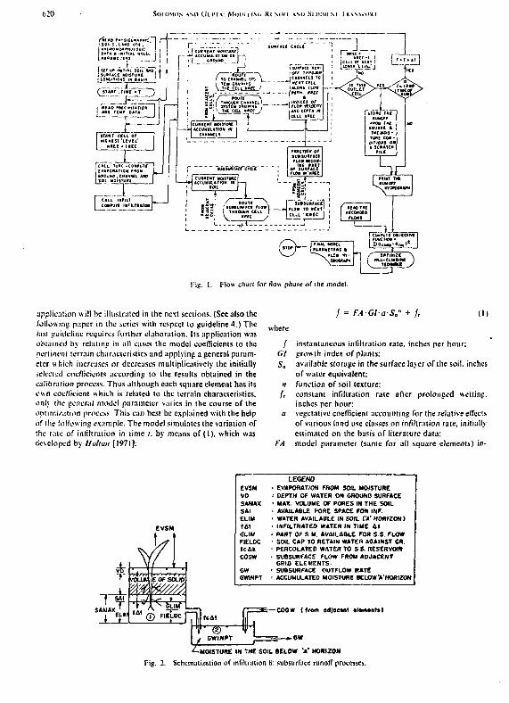
620 S<)l

I SOUS, UNO im .

[ s i n * INITIAL ioit"**o| f tj SJ»»*Ct MOIST LI HI I '(tOWLiiiiOllS tN • V i l " I '

«,M) Cil I'l V M»J1>. 1 !>•<• Kl AOI I

r," _.::.:r _ ^ j «euMuiM^oit7lo» j — i

WEC ilWC

I UM GRftittihS i -1 i[ir HU5 V Till CEIL M R / ALONS KLO«

« I » | 0 M ' O I « I I I M * 1 ' * W I I ' [ CUMCMT HQISTUHCJ ', _ I T PRINT TlLLt"-L«"2J.*i1

li5t-. 1 ' H AceuMutinoM IN — . • * . j ; 1 1 RUN»*

l;ig. I. Flow chart for flow phase of Ihe model.

application will be illustrated in the neit sections. (See also thefollowing paper in the scries with respect la guideline 4.) Thelast j!uiik-linc requires further elaboration. Its application wasobtained by relating in all cases the model coefficients to thencrtini'M terrain characteristics and applying a general param-eter which increases or decreases mulliplicatively the initiallyselected coefficients according to the results obtained in thecalibration process. Thus allhough each square element has itsoun coefficient which is related to the terrain characteristics,onlj the general model parameter varies in the course of theoptimisation process. This can best be explained with the helpof the follow ing example. The model simulates the variation ofthe rate of infiltration in lime ;. by means of (1), which wasdeveloped by Holtan [1971]:

/ = FAGIaSa* + ( I I

where

/ instantaneous infiltration rate, inches per hour:67 growth index of plants:Sa available storage in the surface layer of the soil, inches

of water equivalent:n function of soil texture;fr constant infiltration rate after prolonged wetting.

inches per hour:a vegetative coefficient accounting for the relaliveeffects

of various land use classes on infiltration rate, initiallyestimated on the basis of literature data:

FA model parameter (same for all square elements) in-

LEGCrMOevarosATioN FROM SOIL MOISTUREDEPTH OF WATER ON GROUND SURFACEMAX. VOLUME OF PORES IN THE SOILAVAILABLE PORE SPACE FOX INF.WATER AVAILABLE IN SOIL ("A* HORIZON )INFILTRATED WATER IN TIME AtPART OF S.M. AVAILABLE FOR S S. FLOWSOIL CAP TO RETAIN WATER AGAINST CR.PERCOLATED WATER TO S S. RESERVOIRSUBSLIIFACE FLOW FROM ADJACENTGRID ELEMENTS.SUBSURFACE OUTFLOW RATEACCUMULATED MOISTURE BELOW>'HORIZON

COGW (from odjocint •l«m»nl»)

^-MOISTURE IN THE SOIL BELOW 'A1 HORIZON

Fig. 2. Schcmatizmion of infiltration 8: subsurface runoff processes.

SOLOMON AMJ G I T H : Momusc Rvsvn AM) SMUMIM TK^NM-OKI 621

Fig. 3. Internal water balance for a grid element.

troduced lo account for the error made in initial esti-mates of the values of coefficient a.

For a grid demerit the numerical value of any characteristicwhich is related lo soils or land use. such as Sa, n, (e, and a. isdetermined as the weighted average of the values of the corre-sponding characteristic for different soils or land use typesoccurring in thai grid element. The weighting is done accord-ing to the percentage area of the grid element occupied by eachsoil or land use type. All these values arc kept constant duringthe model calibration. The only model parameter which variesduring the calibration process is FA.

The interfacing of the infiltration subroutine and the flowmodel is indicated in Figures I and 2. This technique ofmaintaining fixed values of the coefficients which relate to thespatially varying characteristics such as soils, land use. phys-iography, etc., and optimizing only the general model paranu-ter which reduces or increases them proportionally makes itpossible to relied in the model the distribution of basin char-acteristics and yet permits maintaining the number of modelparameters at a minimum. This, in turn, results in the reduc-tion of computational effort and cost required in calibratingthe model.

2. Phases of Model Development

Development of the model is carried out in the followingsequence: (I) Reduce data on a square grid reference systemand build up a series of interfaced data files within the frame-work of the derived river basin reference system, includingflow paths of the surface and subsurface water [Gupta andSolomon, 1977). (2) Estimate precipitation and temperaturedata and apply them to each element in the hierarchical orderof computation (determined from the river basin referencesystem), compute losses from the estimated precipitation in-put, estimate the surface and subsurface runoff components,and route them along the flow paths established under step 1.(3) Calibrate the (low phase of the model and determine thecorresponding model parameters. (4) Validate the model intime and space, compare errors of calibration and validation,and check error distribution and lime series: if necessary,modify model to obtain normal distribution and serial inde-pendence of errors. (5) Interface the sediment ero-sion-transportation processes with the pertinent flow com-ponents from the flow phase (overland flow and channel (low)and estimate sediment transport and deposition. (6) Calibratethe sediment phase of the model and determine the parametersof the sediment phase. (7) Validate the sediment model inspace and time, compare with errors of calibration, and checkerror distribution and time series: if necessary, modify model

to obtain normal distribution and serial independence of er-rors.

C. Plow PIMM

The fliw char! of ihe How ph.ise of ihc nuclei is shown -nl:i|Mirc I. The flow pli.ise .nuhsis IS i-.irncil mil fur e.ich ;'iuiclement taken in hicr.inhu-.il order fur c.icii time step Si inttto Mages. The (irsl comets ill e-.nm.ilm>' llie internal w.ilcrbalance for each grid element, .mil the second consists .-Irouting the precipitation excess and inflow Iriun adjacent gridsquares through the grid element (surface .in J siibMirl'.ice rout-ing) (o obtain the total runolT leaving the element. The internalsurface water balance for a grid element | Figure 3) is gi\en b\(2). In the presentation of equations the notations used in thecomputer program are basically maintained in the lev. toenable the reader to readily identify them in the Fortran \er-sion:

(P,\-, + O.SMCOQ,, + COQ,Z) + (FGAi'G,),.,-(£,),-,

- (/i).-> - O.5-SK0,, + 0,2> = (S,2 - S,,) (->

wherep precipitation over grid element / in the interval Si

(external input):F. evaporation loss in the interval St (output esti-

mated as shown in section C2a):COQ Tile of surface flow into the grid element i from

adjacent elements (input from adjacent squares I:FGAVG part of subsurface flow becoming surface flow.

estimated as shown in section CJV (input):/ infiltration loss in the interval Si (output esti-

mated iteratively by the model, .is -.noun in sec-tion C2b);

Q rate of surface outflow from the arid element i.which becomes inflow to the next crid element(output):

S surface storage in the grid element /'. includingstorage due to microrelief as well as storage in thjchannels, estimated by using the Muskincum .as-sumption, section C1.

Index i denotes that the symbols refer to the ilh gnd e1*-menl. Indexes I and 2 indicate that the simboJs refer to :"ebeginning and Ihe end of the time period Si = tii - ; ; i.respectively. Index I - 2 denotes the average quantity over thetime period It.

Inputs in (2) are assumed known. Various possible U'ch-niques of interpolating precipitation and temperature inputs.depending on data availability and terrain characteristics, ueredeveloped by the authors. However, these techniques are out-side the scope of this paper. Input from adjacent squares iscomputed by the model. Losses can be computed as is in-dicated in section C2. The difference (input minus losses) givesthe precipitation excess which is convened lo surface runolfintime Si. The infiltrated water contributes to the subsurfacerunoff. Equation (2) is solved for the outflow unknowns simul-taneously with ihe routing equatiuns described in the nextsubsection.

I. Routing Technique

Routing through the model elements is carried out b> usm,:the Muskingum routing technique as modilicd bv Orcrunt[1970]. Basically. Phe technique reduces to the following equa-tion:

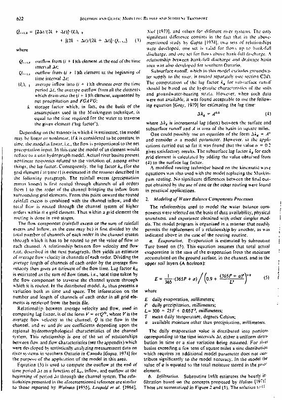
622 SOLOMON AMIGUIMA: MOIHIINC RINUII AM> Si JJIMINI TRANSPORT

[2±t/(2k +•

[(2A - (3)

where

Q,,,., outflow from (/ + 1 )lh clement at the end of the timeinterval Jit;

Q,,:,, outflow from (/ + l)th clement ill the beginning oflime interval Sr,

(/,), , average inflow into (/ + l)th clement over the limeperiod St. the average outflow from all the dementiwhich drain into the(i + I )th element, augmented bynet precipitation and FGAVG;

k storage factor which, in fact, on the basis of theassumptions used in the Muskingum technique, isequal to the time required for the waler to traversethe given element (')ag factor').

Depending on the manner in which k is estimated, the modelma; be linear or nonlinear. If k is considered to be constant intime, the mode! is linear, i.e.. the flow is proportional to the netprecipitation input. In this case lhe model of an element wouldreduce to a tinii hydrogryph model. Actual river basins presentnonlinear responses related to Ihe variation of. among otherthings, the lap factor. Consequently, the lag factor k,, (for thegrid clement i at time r) is estimated in the manner described in;he following paragraph. The rainfall excess (precipitationminus losses) is first routed through channels of all ordersfrom I to the order of the channel bringing the inflow fromsurrounding grid elements. From this point onward the routedrainfall excess is combined with ihe channel inflow, and thetoul flow is routed through the channel system of higherorders within II.e grid element. Thus within a grid element therouting is done in two stages.

The flow component (rainfall excess or the sum of rainfallexcess and inflow, as the case may be) is first divided by thetotal number of channels of each order in the channel systemthrough which it has to be routed to get the value of flow ineach channel. A relationship between flow velocity and flowrale, described in the neM paragraph, then yields an estimateof average How velocity in channels of each order. Dividing theaverage length of channels of each order by the average flowvelocity then gives an estimate of the flow time. Lag factor ku

is estimated as the sum of flow times, i.e., total lime taken byihe flow component to traverse the channel system throughwhich it is routed. In the distributed model. ku thus presents avariation both in time and space. The information on thenumber and length of channels of each order in all grid ele-ments is retrieved from the basin file.

Relationship between average velocity and flow, used incomputing lag factor, is of the form V - ovQ1v, where Cis theaverage Dow velocity in the channel. Q is the flow in ihechannel, and nv and iic arc coefficients depending upon theregional hydromorphological characteristics of the channelsystem. This relationship is one of the set of relationshipsbetween flow and flow characteristics (see the appendix) whichwere developed by statistically analyzing measurement data onriver systems in southern Ontario in Canada [Gupta. 1974] forthe purpose of the application of the model in this area.

Equation (3) is used to compute the outflow at the end oflime period .if as a function of k,t. inflow, and outflow at thebeginning of period -if through the channel system. The rela-tionships presented in the aforementioned reference are similarto those reported by Wolman |I955], Leopold et al. [I964],

.Vic/ 11973], and others for different river systems. The onlysignificant difference consists in the fact that in the above-mentioned study by Gupta (I974J. two sets of relationshipswere developed: one set is valid for Hows up to bank-fulldischarge, and one set for flows above hank-full discharge. Arelationship between bank-full discharge and drainage br.sinarea was also developed lor southern Ontario.

Subsurface runoff, which in this model excludes jroundwa-ler supply to the river, is rouied separately |scc section C2tl).The computation of the lag factor kg for subsurface rutu.ffshould be based on the hydraulic charadcrisiics of the soilsand groundwatcr-bearing strata. However, when such dalawere not available, ii was found acceptable to use the follow-ing equation [Gray, 1970) for estimating the lag time:

Ik, = A° (4)

where AA-, is incremental lag (days) between the surface andsubsurface runoffand A is area of the basin in square miles.

One could possibly use an equation of the form A*, = A"and consider a a model parameter. However, in the appli-cations carried out so far it was found that the value a = 0.2gives satisfactory results. The subsurface lag factor k, for eachgrid element is calculated by adding ihe value obtained from(4) to the surface lag factor.

A modified routing technique based on the kinematic waveequations was also used with ihe model replacing the Muskin-gum routing. No significant differences between ihe final out-put obtained by the use of one or the other routing were foundin practical applications.

2. Modeling of Water Balance Components Processes

The relationships used to model the water balance com-ponents were selected on the basis of data availability, physicalsoundness, and experience obtained with other simpler mod-els. The model program is organized in a manner that readilvpermits the replacement of a relationship by another, as wasindicated above in the case of the routing routine.

a. Evaporation. Evaporation is estimated by subroutineTurc based on (5). This equation assumes that total actualevaporation is the sum of the evaporation from the moistureaccumulated on the ground surface, in the channel, and in theupper soil layers (A horizon):

±/ ( » •

0.9 +(365/M-o)2r (5)

where

E daily evaporation, millimeters;P daily precipitation, millimeters:L = 300 + 25T + 0.057"3, millimeters:T mean daily temperature, degrees Celsius;a available moisture other than precipitation, millimeters.

The daily evaporation value is distributed into portionscorresponding to the time intervals Jit. either a uniform distri-bution in time or a sine variation being assumed. For rnc'basins exceeding a few tens of square miles a sine distributionwhich requires an additional model parameter does not con-tribute significantly to the model accuracy. In the model tl>*value of a is equated lo the total moisture stored in the gi*<"'element.

b. Infiltration. Subroutine Infilt estimates the hourly in-filtration based on the concepts proposed by Holian [19?!iThese are summarised in Figure 2 and (1). The solution tod

SOLOMON *NI> GUPTA: Mcn>i:iiMi R L M I U AM>SH>IMINI TK\NSI'OKI

is obtained by iteration, for each time interval, to balance theconditions (6) and (7) given below:

S,),-2 >SF< 0.5(/M (6)

where

(/',),-j increment of rainfall in time Ar. inches:(Si)i-a depth of water on the ground in transit during Ar.

inches;AF increment of infiltration during Si, inches:St time interval, hours:

!,%. In rate of infiltration at the beginning and end of Ar,respectively.

and

Sal - EVSM + SFC 0)where Sa, and Sal arc values of available storage Sa (equation(I)), in inches, at the end and the beginning of Si. respectively.EVSM is evaporation from the moisture, accumulated in thesoil only, in lime interval Si. EVSM is only a fraction of thetotal evaporation in A/ and is obtained by multiplying the totalevaporation by the ratio of the current soil moisture to thetotal surface and soil moisture accumulation in the grid ele-ment. Parameter SFC = /„'. Si, in which / , ' is the in-stantaneous percolation rate, obtained by multiplying thecomputed drainage rate f, by the ratio of the moisture avail-able above field capacity and the maximum possible fe-av'ta-tional water in the soil, i.e., total porosity minus field capacity.

To initiate the infiltration computations, initial soil moistureconditions are assumed to be given by (8), (9), and (10):

£,, = SAM AX • SOIL DEPTH • (1/100) • VPOF (8)

where SAM AX is total porosity, in percent, and UPOF is thefraction of SAM AX not occupied initially by soil moisture.This is a mudcl parameter and is determined during modelcalibration.

Condition (9) is

EUM = SAMAX • SOIL DEPTH • (1/100) - Sa l (9)

where ELIM is moisture accumulated in the A horizon of thesoil.

Condition (10) is

GLIM = ELIM -FIELDC (10)

where GLIM is moisture in excess of the field capacity of thesoil which percolates to lower layers and eventually contrib-utes to subsurface runoff and FIELDC is field capacity of thesoil.

Updated values of VD, 501, ELIM. and GLIM at the end ofeach time step make possible the computation of the infil-tration rate as a function of the current soil moisture. Also, therecuperation of infiltration capacity of the soil in the period ofno rainfall or very little rain is continually estimated.

c. Surface runoff and channel flow. The total surface run-off from a grid element is assumed to consist of three com-ponents: The first is precipitation excess generated internally inthe grid element, the 'internal runoff." This is routed firstthrough rills and rivulets and then through the major channelsystem of the grid element. The second component is waterwhich flows into the grid element / from the adjacent gridelements, the "external flow" {COQ, in ("igure 3). This is routedthrough the major channel system of the grid element i. Thethird component is the part of the subsurface flow being inter-

cepted by the major channel system in the grid eicmcn:(FGAVG in Figure 3).

d. Subsurface runojj. listimation of subsurface r'jn.vwhich includes groundwater-surface water eu'han^e. riM/j.:.detailed information on the hydraulics of soil .ind gr.-un.waler-bearing strata. As such detailed information is *c:seldom available for large basins, a simplified compel.,;-.approach has to be adopted frequently l-'or basms in M'uthrOntario the available data on surface and grounds atcr ,:r.j ::-terrain cross section indicate that the average t.vr.inbi:iion .subsurface runoff to surface runoff FOA VG at a point can rfairly estimated as

(FGAVG,)^, = (PS + L)W/i00)(GlfOPT), ( I ;

where /. is distance along the main flow path from the has:outlet to the point (grid element in the model) under co;-,-:ceration, Pg is a model parameter to be determined b; ;h.model, and (GH'OPT), is average subsurface outflow from th.yrid element / and is computed as is explained beknv.

In time S(. water available to generate subsurface runoff:given by (12), with reference to Figures 2 and i

GWINPT = (COGIV,),., + Sfc

- (FGAVG,),.,

where

GWINPT

(COGH/,)i-J average subsurface inflow, during lime A;

Sfc{FGAVG,),.,

water available to become subsurface runinches:average subsurface inflow, during limefrom adjacent grid elements, inch;.1*:percolated water during time A/, inches:average contribution of subsurface w.t:srsurface water, inches;subsurface water in storage at the beginr.:::of time period Si. inches.

(GU'OPT), is obtained by routing <7»7 \7'7' through :he f.-ielement in a manner similar to that of the surface water b..with a larger lag. the difference between the surface anil Osubsurface lag being given by (4). {GH'OPT), becomes ^ p_rof (COGlV)l_2 for the grid element being fed by grid eleinen'. i.

D. SEDIMENT PHASE

The sediment erosion-transport model is interfaced »l'.h '.hflow phase of the model through the estimated runoff an J i.ccharacteristics (flow velocity and depth) obtained from :.-flow model. The flow characteristics are obtained b> uur.z •:.relationship between velocity and flow, mentioned in *t;:;iCl , and a similar relationship between depth and flow iC<-'and Solomon. 1973). given in the appendix. Ir: tr.e node. ;•.total sediment discharge from a grid element :n one .:":.period is assumed to consist of two parts' The first k >ed.:r.;discharge generated within the grid element bv land en."- >processes, i.e., by action of rainfall and overland flow w•.•.!:•the given element or in the upstream elements draining snto :.-given element: this is mainly the suspended sci'imcm portio1

of the total river sediment. The secund part is sediment Uv.generated by erosion of the channel cross section, i.e.. by i'r.~channel flow. This sediment load represents m;-inl> bed .^.:JThe channel flow also carries the suspended st.ii.i:er.t ;.:;•.*•:•ated in the upstream elements to the extent it was no: dera -iled because of low velocities. The possibility that depo-iuosediment.'! become again part of the sediment liifch-.irire «!:-•:•velocities (flow) increase is also considered in ihe moiiei !'"-•

AM) (JUIMA: MODI I ist. Ki MHI AM* Si MI.MI M I H'.\\rnKJ

r~

!i ii<c*.«"f7] __JWA"i.«3r| (ToiiV-iiiWfSoif—I

Fig. 4. Flow chart for sediment phase of the model.

flow churl for lhis phase of the model is shown in Figure 4. Thefolliming! sections describe the considerations that were usedlo develop the sediment model algorithm and the correspond-ing computer programs.

1. Si'ilimenl Eroded From Land

Land erosion is simulated by the following four separate butinterrelated processes: (1) soil detachment by rainfall, (2)transport of detached sediment by rainfall, (3) sediment de-tachment by surface runoff, and (4) transport of detachedscdiinent by overland flow. Each process is simulated in themodel by a simple scinicmpirical relationship based on theevidence presented in the literature on the relation betweenthese processes and ihe model inputs (precipitation), systemcharacteristics (soil erodibility, land use, and land cover), andoutputs from the flow model (velocities, depths, and flow).

a. Soil detachment by rainfall. On the basis of studies byEllison (1944a. b\. Linsleyet al. [1958], Oniselal. [1958], andFree [I960] this process is simulated by (13):

DR = SDR-SOILE-\}SVe-(P\USVr-(AREAnaaa)-SAVF

(13)where

DR amount of soil detached by rain, tons;SDR a model parameter taking care of the units and the

absolute value of the soil detachnbility under theprevailing land use conditions: this is a model pa-rameter and as such is evaluated during modelcalibration:

SOIl.h weighted average of the relative crodabilily indicesof soils in a grid element (determined by the tech-nique proposed by Wischmeier el al. [1971]); ihe

weighting is done according to the percent of areaof each grid element occupied by each soil type:

USEF weighted average of the land use factor (acoefficient designating the relative effect of land usetypes on the quantity of sediment detached, otherconditions being equal): weighting is done accord-ing lo ihe percent of area of each land use type, andsuggested values for VSEF are given in Table 1:

PMISV nel rain. i.e.. rain per hour after s . ' trading evapo-ration and infiltration losses:

AREA area of the grid clement, square feet:SA VF a sediment availability factor.

SA VE is estimated by the following equation:

SAVF = (So - Sc + RCt)/Sc

in which

So average annual sediment yield of the element in tonsestimated from average sediment yield maps such as theone given by Stichling [1973]: as the value of .?„ is usedin a ratio in which both the numerator and denominatorare practically proportional to it, an error made in itsestimate is of no consequence;

Sr total accumulated amount of sediment which has goneout of the watershed element from the start oi'the modelrun to the current time period:

RC average rate of sediment generation from the watershed(computed from 50) for the lime span of model run:

t total time from the beginning of the model run.

b. Soil detachment by internal runoff. This is estimated by(14) on the basis of the assumption that the quantity of sedi- .ment detached by the surface runoff is proportional lo tin" ,'

SOLOMON AM> G I T I A : MOIN I IM. RI MM i AND SI imu M

TABU: I. Siifpcslcd Values of Land Use Factor USht

Land Use 1 ype USE?

Crop land (cwcpl forage)L'rhani/ed landQuarries and sand and gravel pitsOrchards and vineyardsHorticulture and fur and poultry farmsRough grazing and range landImproved pasture and forage crapsRock and other unvegctated areasWater, swamps, marshes, and bogsOutdoor recreationSand flats, dunes, and beachesWoodland

t.O0.40.80.150.60.60.40.250.00.50.50.04

tractive force exerted and on the basis of the relationshipsproposed by Meyer [1965| for the flow velocity in rills andrivulets:

DF - SDF-(SLOPE-QI!HTf-VSEF-SAVF (14)

where

OF sediment detachment, tons per hour:SLOPE average slope of the grid element:

QINT total flow corresponding to the surface runoff,inches of runoff over the grid element flowing intime (, converted to flow units:

SDF a model parameter similar to SDR.

c. Transport capacity of rain. The transport capacity ofrain is estimated onUhe basis of the studies by Ekern [1953)and Rowlison and Manin [1971) by (15):

TR = STRSLOi>EPMlSVSAVF (15)

where TR is the transport capacity of rain, in tons per hour,and STR is a parameter similar to SDR.

d. Transport capacity of surface runoff. Findings by Laur-sen (1958) and the experimental results of Meyer [1965] sug-

gest a relationship of :!ic form of (l<>) for csiini.uini; thetransport capacity of the internal flou component.

TF - STF-SAVF-\QlST-SI.OI'Ef ' (16)

where TF is the transport capacity of the inicm.il flow com-ponent, in tons per hour, and STF is a model parametersimilar to SDR. In one time period the toial amount ol de-tached sediment available for transport to the major channelsystem TOTDSD is given by

TOTDSO = DR + DF * USED l l " )

where DSED is the amount of sedimeni left over from theprevious time interval.

Total transport capacity of rain and overland flow TO1CAPis

TOTCAP = TR + TF (IS)

In any lime period, if TOTCAP 1 TOTDSD. sediment fromland erosion is equal to JOTDSl). and if TOTCAP -,TOTDSD. a sediment amount equal to 1OTCAP IS trans-ported from rills and rivulets to the major channel s\slcm andthe balance DESED becomes available (or transport in thenext time interval. The sediment delivered to the nujor chan-nel system is transported out of the grid element by the totalflow in the channels.

2. Sedimeni Erosion and Transport in Channels

The average concentration of the bed sedimeni. b> weight(i.e.. the ratio of sediment discharge to «v.ier discharge i. :,-.;.-.>-ported out of a grid element is estimated b; (19). which i*based on the theory of sedimeni transport proposed b\ Gat-cliarov

(19)

5 3 "•"-j & 0.'£§ 0.8

H

500

| 400

2 300

IU- 200

100

0 1 1 1 1 1 1

w.

t

LH

> i i i

—

• U - D

Measured

Synthesized

LJ

I 3 9 7 9 II 13 IS IV 19 il 23 3 27 29 311 2 4 6 6 10 12 14U MAY '68 J - JUNE '68

Fig. 5. Synthesized flow by model and measured flow at O2HCOO3 (Weston): model calibration

626 N A M J G I T I A : M C I D I I I M , K I N U I I A N D N I D I M I M T U W M M I K I

•* cr QO

2 5 0

u 150

u QJ

• Measured

Synthesized

2 4 6 8 10 12 14JUNE '68

Fig. 6. Synthesized flow by model and mcusurM flow ;n O2HCO25 (tldcr Mills): validation in space.

where

RUOVTPHI

D1AM

bed sediment concentration by weight;a turbulence parameter, whose value dependsupon the representative particle size of the sedi-ment and is given b> Cnncharov [1964];representative particle size of the sediment, com-puted as the weighted average of diameter valuesobtained from the grain si/e distribution curves ofSOHN occurring in the given element, millimeters;average How velocity in the grid element, millime-ters per second; this is computed as an average ofthe How velocity in channels of order StORPIN toSR1Y of the grid element, where A'rt/l' is the'order" (as defined by Sirahler [l%4]) of the majorriver channel draining the given clement andMORDIS is the order of the major channel bring-ing the channel (low from the adjacent grid ele-

ments into the given element; these orders areobtained from the model data bank described byGupia and Solomon [1977]; V is computed usingthe hydromorphologic relationships described byGupia and Solomon [1373];

H average Mow depth in the channels having orderfrom MORDIS to NR1V. computed in a mannersimilar to that of computing V. meters;

''„ nonsilling velocity, corresponding to the represen-tative grain size of the bed sediment, meters persecond.

Y\ is estimated as

where •>, and 7 arc specific weights for sediment particles and

°8

300

— 200

U r u u U

Measured

Synthesized

15 17 19 21 23 25 27 29 I 3 5 7 9 II 13 15 17 19 21 23 25 27 29 31L JUNE '68 - U JULY "68 ~

Fig. 7. Synihcsized flow by model and measured flow at O2HCOO3 (Wesion): validation in lime.

SOLOMON ANPGUPIA: Mimi-UNu KUNOII AMISIUIMIM THWM-OKI 627

2O

ao

LO

IME

NT

t

to

400

350

300

250

200

ISO

100

50

"TJ

-

U

II

/

jJ IP,

h i

A iA}\

i\t

i

i

an

- Measured

- Synthesized

_^

00 s to.s|y

I 3' 5 7 » II 13 IS 17 19 21 23 25 27 29 31 2 4 E B 10 12 14f» MAY "68 4- JUNF '68

Fig. 3. Synthesized sediment load by model and measured sediment at O2HCOO3 (Weston): model calibration.

water, respectively, and a, is a coefficient, equal to 3.5 forsediments in the range of natural sands and silts.

The total bed load carrying capacity of the channel flow inthe grid elements BLOL'T is computed as the product ofRHOVT and the external flow components as defined in sec-tion C2c. This is compared with the bed sediment loadACBLOD remaining from the previous time interval Ar in thegrid element, ir ACBLOD 2 BLOVT. the amount (ACBLOD- BLOVT) is left behind in the grid element (deposition) andis considered again in the next time period. If ACBLOD <BLOUT. the balance is assumed to be picked up from thechannel cross section (scouring).

According to Goncharov [1964], (19) and (20) are valid for

both the "ridge and ridgeless phases.' i.e., flat bed and bed withripples, dunes, etc.. of the channels, and the values of empir-ically determined constants and parameters in the develop-ment of the equations are valid for a wide range of Howconditions in natural channels transporting sediment.

E. MODEL CALIBRATION AND VAI IIHTIOS

The flow and sediment phases of the model are calibratedseparalely on a watershed (to determine the .alues of themodel parameters for the watershed) using the measurementson How and sediment discharge made at hydromeiric stationsin that basin. A measure of the model performance is obtainedby computing the error variance given in (21):

is I o.o u LJJ LJJ

: iso

Meosured

Synthesized

I 3 5 7 9 II 13 IS 17 19 21 23 25 27 29 31 2 4 6 6 10 12 14

Fig. 9. Synthesized sediment load by model and measured sediment at O2HCO25 (Klder Mills): validation in space.

62S JNC' Kl'NOI I ) Si DIM! M TK4\M'ilKt

IT

MeasuredSynthesized

in IS 17 19 21 23 25 27 291 I 3 5 7 9 II 13 15 17 19 21 23 25 27 29 31

E:ig. 10. Synthesized sediment load by model and measured sediment load al O21ICOO3 (Wcslon): wttidtition in time.

(21)

where Q,m is measured flow-sediment load for the /th day, Q,,is synthesized flow-sediment load for the rth day, and N isnumber of days for which the model is calibrated.

The parameter values which result in the minimum P aredetermined by subjecting the model to an optimization com-puter program C1.1.U8, which is based on Rosenbrock's hill-climbing search technique [Rosenbrock, I960]. After determin-ing the model parameters for the calibration watershed andtime period. Ihe model is validated in lime by running it foranother lime period and in space by running it for a sub-waicrshed of Ihe river basin. A comparison ofthe errors of\;ilitkuion and calibration indicates the acceptability of themodel. If the errors of calibration arc acceptable (by com-parison with measurement errors and errors in input andoutput), the model can be considered acceptable if validationand calibration errors are of same order of magnitude. Resultsof the calibration-validation tests in the H umber River insouthern Ontario are shown in Figures 5-10. As was noted bySolomon [1975], further indications on the acceptability ofthemodel are ihe closeness of the error distribution to a normalone and the serial independence ofthe errors. A more detaileddiscussion of the calibration-validation results, including ananalysis of ihe optimized model parameters, is included in theihird and last paper of the series.

APPENDIX: HYDROMORPIIOI.OGIC RELATIONSHIPS FOR

KIVFRS IN SOUTHERN ONTARIO

The hydromorphologic relationships developed for the riversystems in southern Ontario are as follows:

where QI*F is discharge in cubic feet per second at bank-fullconditions and A It is drainage basin area in square miles aboveIhe point at which channel dimensions are being predicted.

Within-the-bank flow conditions

A = 5.790°"V = 0 .270" '

i r = 21.160°»D = 0.310°"

Over-bank How conditions

A = 14.390°"V = 0.460° •"W= 85 .100"D = 0 .570°"

where

0 discharge in the channel, cubic feet per second:A area of cross section, square feet;y average Mow velocity, cubic feet per second:

H' surface width of flow, feel;I) average deplh of flow. feet.

For each relationship the coefficients and exponents were sta-tistically derived by analysis of actual measurements ofgaginfstations. Because of this reason the sum of the c\ponents urthe product does not come out to be equal lo unity, a require-ment of the law of continuity.

REFERENCES

Ekcrn. P. C . Problems of raindrop erosion..4 gr tug.. JJ(] )• -•'• I"';1

Ellison. \V. D., Studies of raindrop erosion. Jgr. Eng..24(4). 131 — 1 -~'-1944a.

Ellison. W. D.. Studies of raind-op erosion. Agr. Eng..24{5),]M-l>'1944/1.

Free. G. R.. F.rosion characteristics of rainfall. Agr. Eng.. *t*4J7-149. 455. I960.

Goncharov. V. N.. Dynamics of Channel Finn: translated from Ri-'siun b\ Israel Programme for Scientific Translations. Oldhnur'.PriiMS. London. 1964.

Gra>. D. M.. Principles "I Hydrology. Canadian Committee fur :•' =International H.vdrnlocical Decade. Secretarial. Canada. 19•(•

Gupla. S. K.. A distributed digital model for estimation of fUm% ;

wdinicnl load irom laruc uncanped watersheds, Pli.D. IIK'SIS. 1 '•• ••ol Waterloo. Waterloo. Onl.. Canada. 1974.

Gupia. S. K.. anJ S. I. Solomon. Transfer techniques for «d"''>'dul;i, 1'luvijl Processes and Sedimentation. I'roc. Can H* ••'_'.Suiip. '). Univ. ofAlberta. l:dmonlon. Alhcrta. Canada. Ma> I"

IMC

/'.-•ni

pr-.

ih i i

,.k.,1. | ' l

1 Jl.UCf

1 ••

SUl-OMON AND GUI'TA: MOUli.ING Kl 'NOIt AND SlIIIME NT TKANSI 'OK ' I

Ouptii. S. K.. and S. 1. Solomon. A distributed numerical model Tor Rosenbrock, H. I I . . An automatic method for tmilimestimating runoiVand sediment discharge »•(" unpaged rivers, t. The lea.sl value of a function. ('mnput. J.. J. 17S, i»jf,oinformation svstcm. Water Resour. Hex.. IS. ilii> issue. 1977. Kouiison. 1). [... and ( i I M.irun, K.tiinn.tl in.iild i

Holl.in. I I . N., A formulation for quantifying the influence of soil erosion. J. /m i : l)ttwi, />/r -Inter S<u ( ml In-.'.piuosity and vegetal ion on infiltration, paper ptcseutcd at the Thin! Solonum. S. J., i'onmu-tcr ti<xi"tiiilKttiuni ./•(./ \i7«.>/-International Seminal for Hydrology Profcnsors, Purdue Univ.. \2, Institute on Shich.iMic Mcthml^ HI H\di.'!,-.j\ .vn:I afayeltc. Indiana. July 18-30. I1J7|. sources. Colorado Stale I'mversiu. I »n i. MU:\s.\ .»!.« . I " "*

(..'lurscfi, V- M., The tolal sedintenf loads of streutm, J. ihtlruuL Dm. Siichliiif*, W. {"., Sediment loads in i'.uuuii.in nu-: \ . \ !-.:v!.u !':>,..%-.•.Atm-r. S,n. Civil hug.. W(HVI) . 36. 1*>5S. and Sedimentation. / W ( .;/; HvJn>l S\ ••:;• -J f t m o( \ihcr:.i

Leopold. L. B., M. (1. Wolinan, and J. V. Miller, t'luvia! Processes hi tidmonion. Alberta, Canada. M.iv I1'™ •Ceowarpltofajtv. p. 32K. W. H. Freeman. San t-'ranciseo. Calif.. Slrahler. A. N.. Quantitative gcomorphoUii^ r\ iir.un.ii!c KIM".-. ,ii\]1%4. channel network*., in Handbook u! 4pr.uJ ihJwt-av. ediied :•"•

l.insley. R. K.. M. A. Kohler.and J. L. H. Paulhus. Applied Hydrology. V. T. Chow. sect. 4-11. McGraw-Hill. \ e » V.*rk. WM•115 pp.. McGraw-Hill. New York. 195S. Wischmeier. \V. H..C. B. Johnson, and B V. Cross. A soil eroiij.hih;\

Meyer. L. D.. Mathematical relationship govern soil erosion by nomograph for farmland and construction sue*. J. Soil Water C '>»;•water. J. Soil Water Cnnsen:, 20. 149-150. 196.. sen:. 26. 189. Scpt.-Oct. 1971.

Neil, C. R.. Hydraulic geometry of sand rivers in Alberta. Fluvial Wolman, M.G.. The natural channel of Brandy Wine Creek. Penrml-Processes and Sedimentation. Proc. Can, Hydrol. Symp. 9. Univ. of vania. U.S. Geol. Sure. Prof. Pap., 271, 1955.Alberta. Edmonton. Alberta. Canada. May 1973.

Oltis, T.. T. O. Laws, and D. A. Parson. Relation of raindrop size tointensity. Eos Trans. AGU, 39(2). 205-291. 1958. (Received July 29. 1976:

Overton. D. E.. Route or convolute. Water Resour. Res.. <S(1), 43, revised February I I . 1977:1970. accepted February 22. 1977.)

APPENDIX 2, PART II: MODEL CODE A2,l

-BASIN MODEL.

MODIFIED VERSION. BY MING LEE. OCT. 1976.

CARD IMAGE T.TTI..!L FOR THIS RUNFRACTION OF GROUND WATER OUlFLOW WHICH BECPilK!:;BASE FLOWINITIAL AVAILABLE STORAGE IN SOU... INCHESUSED TO INITIALIZE GROUND WATER STORAGE AND GROUNDWATER OUTFLOW. INCHES OR INCHES / HOUR RESPECTIVELYSCALING FACTOR APPLIED TO VALUES OF FC IN MASTER FITRAVEL TIME FOR GROUND WATER FLOW WITHIN SOUARE. HOSCALING FACTOR APPLIED TO CALCULATED TRAVEL TIMEFOR OVERLAND FLOW WITHIN THE SQUARESCALING FACTOR APPLIED TO CALCULATED TRAVEL TIMEr-OR CHANNEL FLOW WITHIN THE SQUARESOIL THICKNESS. INCHESSNOW THICKNESS. INCHES* WATER EQUIVALENT) IF AMY.BASIC TIKE INTERVAL. HOURSNUMBER OF SQUARES IN SUB-BASINMODEL STARTS WITH 'INLYR' YEAR.MODEL STARTS WITH 'INMTH' MONTH.MODEL STARTS WITH 'INDAY' DAY.BASIN 13 MODELLED FOR NDAY CONSECUTIVE DAYSMAXIMUM NUMBER OF SUBDIVISIONS OF BASIC TIMEINTERVAL. 'TIME-IN'SET TO 1 FOR OPTIMIZATION BY 'CLIMBX". 0 OTHERWISEWORD IN MASTER FILE CONTAINING INFILTRATION CAPACITWORD IN MASTER FILE CONTAINING 'IURBAN'INCHES / HOUR / INCH OF AVAILABLE STROAGENUMBER OF SQUARES FOR WHICH RESULTS ARE TO BE PRINTSUBSCRIPT NUMBER OF SQUARES FOR WHICH RESULTS ARETO BE PRINTEDRECORD NUMBER OF RECORD IN MASTER FILE FOR EACH SOUIN THIS SUB-BASINSUBSCRIPT NUMBER OF SQUARE THIS SQUARE FLOWS INTO

INTEGER WKSTO R(443)INTEGER ITITLE( 4CO.L00KSCK5 ).NREC<203 ).NXTSQ< 203 )REAL GMESD* 200»5 )INTEGER IREC*2000>LOGICAL OUTPUTCOWIQN/AREAl/GWFRAC.SAl'NIT.GWINIT.FCFRAC.GWLAG.fcSFDLAG.SFCLAG.SOILT.NSQ.MAXDIV.1NYR.INMTH.INDAY.NDAYS.*I OPT. NLOOK .LOOKSQ. NREC.. NXTSQ. OUTPUT, TIMEIN. NPRIME.* GRID.NHOUR.IQUTEQUIVALENCE ( WKSTOR( 1 ).GWFRAC)CALL FGT.TM< IHRO. IMINQJ.SECO )

ACCEPT 'ENTER 0 IF DIRECT OUTPUT ON PRINTER IS DESIRED....'.!IOUT=12:I:F<I.EQ.O>GO TO 1991I0UT=25CALL DELETE* 'GRID.LS'.0.IER)CALL OPEN*25.'GRIO.LS'.O.IER)

1991 CONTINUECALL OPEN( 18.'GRIDINPUT'.0.1ER)ChLL OPEN* :l 9. ' MODEL ,. WO' . 0. IER ) r

CALL 0PEN<21.'MASTFI'.0.IER.300)CALL DELETE* 'GRIDOUTPUT'.0.IER )

ccccccccr*cccccccccc:ccccccccccccc

TTITLEGWFRAC

SAINITGWINIT

FCFRACGWLAGSFOLAG

SFCLAG

SOILTSNOWTTIMEINNSQI NYRINMTHIN DAYNDAYSMAXD.IV

I OPTIWRDLIWRDI

NLOOKLOOKSQ

NREC

NXTSQ

A 2 , '/

CALL OPENC 2 2 - 'GRIDQUTPUT ' . O.IER )DO 1.711 1 = 1.5

1711 LOOKSQ(I )=OREAM I S . 5 0 0 MTITLEREAM 1 8 . 501 >3AIWIT.FCFRAC..GWFRAC.3FCLftG..GWIHIT.GWI...AG,SF0LAG.

* SOILT.SNOWT.TIhEINREAM 1 8 . 5 0 2 )NSQ.INYR.1NMTII.INDAY,NftAYS.MAXDIV..I OPT.MPRIMEREAD< .1.8.502 >NLOOK.<LOOKSG< I J ) . IJ-.1. .NLOUK >k'EAi.i( 1 8 . 5 0 2 X NREC< ISO KNX.TSCK ISO >.ISCt»l „ N3G )CALL RBRW<21.0.IKEC.1.IER )GRID~IREC<4)/1000.WRITE<I OUT.600)IHRO.IMINO.ISECO.ITITLE.* INDAY.INrtTH.INYR.NBAYS.TIMEIN.MAXMUNSQ.

* IREC( A ) . IREC(4 )WRITE? IOUT.601 )SAINIT.FCFRAC.GUFRAC.SFCL.AG.GWINIT.GWLAiS.SI-'OLAG. SOIL! .

* SNOWTWRITE(IOUT.602 )IOPT.NLOOK.< LQQKSQ<I ).1-1.NLOOK)

BO 3 ISTN--1.NL00KREAJK 1 8 . 5 0 4 )( QMESD< JH. ISTN ) . J H = 1 . NHOUR )

504 FORMATC12F3.0)WRITECIOUT.5041) (QMESEK JH.ISTN ).JH=1,NHOUR)

5041 FORhAT(1X.&F10.2)DO 2 JH=1.NHOUR

2 QME3IK JH. ISTN )=QMESD< JH. ISTN )/( GRID*GRIEi*249 .1646 )3 CONTINUE

WRITE BINARYt 22 )NLOOK.NHOUR.(< QMESD( JH. ISTN ). J 1-1 = 1 .NI-IOUR >. ISTN=1 .Ni.OG;;C IF<I0PT.NE.1)G0 TO 10C NVR = -NVARC NCON - NVARC NFIG = 4C IWORK = 100C KURT = -1C INDEX = 2C OUTPUT •-• -FALSE.C CALL CLIMBX(NVR.X,NCON.SERRSG.NFIG.WORK.IWQRK.KWRT.G.H.INDEX.C iHNTRIPV.DRBRMy.IER)C 10 CONTINUE

OUTPUT = .TRUE.WRITE BINARY( 19)WK8T0RCALL RESETCALL SWAP( 'M0DELS1.SV'.IER)CALL FGTIM<IMR.IMIN.ISEC >WRITE( I0UT.699)IHR.I«IN,ISEC

500 FQRMAK40A2 >501 FORMAT(14F5.0)502 I"ORMAT( 1415)

600 FORMATdHl.'««#** DISTRIBUTED MODEL NOVA VERSION 1.0 '.* 10X,I2.':',I2,':'.I2,30X.' MODIFIED BY MING LEE « » * * ' /*1H-.1OX,4OA2/

*1H-.1OX,'MODELLING STARTS AT '.12.'/'.12.'/19'.I?.' FOR '.* ' DAYS'/*1H--.1OX. 'BASIC TIME INTERVAL IS '.F3.1.' HOUR'/*1H0.10X.'MAX. NUMBER OF SUB-DIVISION OF BASIC TIKE INTERVAL IS '.* 1 2 /* 1 H O . 1 O X , ' S I Z E OF THE SUB-BASIN I S ' . 1 3 . ' GRIDS ( ' . 1 4 , ' M * ' .* 1 4 . ' M ) ' )

601 FORMAT(1H-.10X.'INITIAL MODEL PARAMETERS :'/&1H0.12X, 'SAINIT ••= '.F12.5/:|-1 HO. 12X. ' FCFRAC = ' , F 1 2 . 5 /

6 C

699

*1IIO. 12X•MII0.12XJR1.H0.12X*1HO.12XJKlH0,12X*1I IO.12X:!!.UI0r12X

FURMAK*1HO,12X«1H-.1OX;i;:l.HO.:l. OX

FORMAKCALL RE!STOPEMU

.'GWFRAC ==

. 'SRXAG -

.'GUIJWIT =, ' LiyLA(3 =. ' EII-ULMG =

.'GD1I...T =

.'SNDWT =1H1/1.H-.10X. ' I O P T ~ '

' .1- 12.5/'. . F12.5/' .F12.5/'.F12..5/' .F12.5/' .F12.5/' -F12.5/ ).'RUN TIME PARAMETERS:'/.12/

.'HYDRO-GRAPH TO BE GENERATED FOR ' . 1 1 , '

. 316 )1H1. ' « « «SET

NORMAL TERMINATION: ' . 1 3 , ' :

SQUARE(S)

'.12.' : ' . . I

A2,4

OVERLAND INFLOW RATE AT BEGINNING OF TIME PERIOD.INCHES / HOUROVERLAND INFLOW RACE AT END OF TIME PERIOD.INCHES / HOUROVERLAND OUTFLOW RATE AT CF.G INNING OF TIME PERIOD..INCHES / HOUROVERLAND OUTFLOW RATE AT END OF TIME PERIOD.INCHES / HOURCHANNEL INFLOW RATE AT BEGINNING OF TIME PERIOD.INCHES / HOUR-CHANNEL INFLOW RATE AT END OF TIME PERIOD.INCHES / HOURCHANNEL OUTFLOW RATE AT BEGINNING OF TIME PERIOD.INCHES / HOURCHANNEL OUTFLOW RATE AT END OF TIME PERIOD.INCHES / HOURGROUND WATER INFLOW RATE AT BEGINNING OF TIME PERIOINCHES / HOURGROUND WATER INFLOW RATE AT BEGINNING OF TIME PiiRIQINCHES / HOURGROUND WATER OUTFLOW RATE AT BEGINNING OF TIME PERIINCHES / HOURGROUND WATER OUTFLOW RATE AT END OF TIME PERIOD.INCHESAVAILABLE STORAGE IN SOIL AT END OF TIME PERIOD.INCHESMAXIMUM VOIDS IN SOIL. PER CENT OF BOIL THICKNESSCONSTANT RATE OF INFILTRATION AFTER PROLONGEDWETTING. INCHES / HOUR * 1OOO.FIELD CAPACITY OF SOIL. IE. MAXIMUM AMOUNT OF iJiVLiRTHAT CAN BE STORED IN SOIL AGAINST GRAVITY.PER CENT OF SOIL THICKNESSNUMBER OF SQUARES DRAINING THROUGH THIS SQUARE

COMPILER NOSTACKREAL SAMAXC 203).FCWRD< 203).ELIM( 203KSAK 203).GLIM 203).

* FIEI_DC< 203)REAL TEMP.PRECIP< 203).REC5( 203)REAL SFSTOR< 203>.GWSTOR< 203).SF0UTl( 203 ) .

* SFINCK 203).SFINC2< 2G3>.GWINC1< 203 ).GWINC2< 203)REAL OVINFK 2O3).OVOUT1( 2O3).CHINF1< 203 ).CHGUT1( 203) .

« GWINFK 203KGW0UTK 203)REAL INF. REC( 1 4 ) . QI_OOI« 5 . 1 0 ) . QLKX 5 )DOUBLE PRECISION DTEMP.DPREC.DTAC.DEVAPREAL LUSE< 203)INTEGER LOQKSCK 5 ).NREC( 203),N.XTSQ< 203)INTEGER IURBAN< 203) .W0ST0R<443)LOGICAL OUTPUT.TEST1.TEST2.URBANCOMMON/AREAl/GWFRAC.SAINIT.GWINIT.FCFRAC.CiWLAG.

* SFOLAG.SFCLAG.SOILT.NSQ.MAXDIV.INYR.INMTH.INDAY.NDAYS*.IOPT.NLOOK r LOOKSQ.NREC.NXTSQ.OUTPUT.TIMEIN.NPRIME.* ' GRID.NHOURMOUT

COMMON / X I N I T / REC5EQUIVALENCE < GWFRAC.WOSTOR< 1 ) ).( OVINFK 1 ).REC5( 1 ) )CALL OPEf-K 19,'GRIDTEMP' ,O. IER)CALL OPEN(20.'GRIDPREC'.0.IER)CALL OPEN(21. 'MASTFI ' .0 . IER.300)CALL OPENC 22. 'MODEL.WO',0,IER)READ BINARY ( 2 2 ) WOSTOR'

cp\.I

r;

CCCCCC[..

ccccccccccccccccccccccccc

07INF1

0VINF2

0V0UT1

0V0UT2

CHINFJ.

CHINF2

CH0UT1

CH0UT2

GWINF1

GWIN.F2

GW0UT1

GW0UT2

SA2

REC6REC7

0.8*REC6

REC4

IIIIIIIIIIIIRIIIIfln

A2,

CALL CLOSE*22.IER)CALL APPEND*22.'GRIDOUTPUT',0„IER)IF< I0UT.NE.12 >CALL APPEND', I OUT . 'GRID..LS ' .O . IER)

C * X11 * * * * * * :K::: * * * * * * * * * * :l: .i ;S« * * •'•• * * % * * « * * * * -!' t £ * 5 * * * * -R ;!'•.:: ¥ r * •!•: * tf :« V * "* '•'. ".Xt % •>• * *Cc VARIABLE TIME STEP FACILITY BASED ON IHI:: FLOU AT THE ' MOUTH'C. OF THE 8UBBASIN TO DETERMINE WHETHER THE TINE STEP iJHOULIi 1:1::C SPLIT OR NOT.CC * ** * * * * * t * * * * X1: -1: * * * * * * * * * * * * * * $ * * * * * * * * * * * * * * * * * t * \-1 * * * * * * :|: M ;|: :|: :i: -|: * :|; * t * *

UKiE«AN=H.IRBAfK NSQ ).EQ. 1CALL RETVE(REC5.5,NREC.NSO)DO 2 ISO--J..NSBIURBAhK ISQ )=0IF( REC5CISQ ) .GE.O. )60 TO 2

KEC5< ISQ )=AESC REC5< ISQ ) )LUSE*ISO )-REC5( ISQ>/100.DO 3 IDAY=1.NDAYS»O 3 ILOOK=1.NLOQKQLOOK*ILOOK.IDAY ) = 0 . 0I LOOK = NLOOKITR » 1JHOUR-0IDATE = 1I. DATE - 0I HOUR »» 1I DAY "<INMTH-1 )*30+INDAY+INMTH/2LDAY'= 0IDIV ~ 1NJJIV ~ lAXDIVOT = TIMEIN/FLQATtMAXDIV)IBWICH=1:I:F(NPRIME.LE.O)GO TO 245

DT==TIMEINDTLAST ~ DTSFINF=0.9A02CALL RETVE* REC5.6.NRECNSQ )DO 5 180=1.NSQUVOUTKCHIWFKC HOUTK.GW.TNF.1.(SFOUTKSFINCKSFINC2*QWINC1*GW1NC2CSFSTOR<SA1* ISQ

ISQISQISOISOISQISQISQISQISOISQ) =

))))))))))

= 0.0- 0.0001= 0.0= 0.0= 0.0= 0.0= 0.0= 0.0= 0.0= 0.2

SAINITSAMAXCISQ> = R E C 5 ( I S Q ) / 1 0 0 . * SOILTFI.ELDC< ISQ ) = SAMAX( ISQ >*0.8ELIM(ISQ) = SAHAX(ISQ) - SAINITGLIM(ISQ) - 0 . 0I F (ELIH(ISQ) .LE.FIELDC(ISQ ) )G0 TO 211GLIMCISQ ) = ELIMtISQ >-FIELDC(ISQ )ELIM(IEU) = FIELIC<ISG)

211 CLIM(ISR) = GLIf-i< ISQ) + 3 0 .5 CONTINUE

A2,6

3 0 1

S02

CALL RETVEC REC5.7.NREC.NSQ)00 501 ISQ==1.NSQFCWRDi ISO )==REC5( ISQ >/1000.*FCFF-:ACCALL RETVEv REC5.4.NREC.NSQ )HO 502 ISQ--1.NSQGWOUTK ISQ >=( REC5( ISQ ) + l. )*GWINITGWSTOR<ISO ) = 41.*GWOUT1(ISO)OVINFK ISQ>==0.0

Ccc SET UP THE TEMPERATURE

ALSO. CHECK THE DATEAND PRECIPITATION FILE

CALL SETMETC INYR. INMTHNXTSCK NSG ) = NSQ + 1:;;FINC2< NSG-U > ~ o.oGU:I:NC2( NSO-U ) = o.o

INDAY.NDAYS.NSQ.TcMP.PREC'CP )

CC SPECIFIED THE FOLLOWING VARIABLES TO INVOKE THE VARIABLE TIMEC. SPECIFIED THE FOLLOWING VARIABLES TO INVOKE THE VARIABLE TIMEC. STEP FACILITY.C HAXDIV GREATER 1 TO INDICATE THE MAXIMUM NUMBER OF SUBDIVISIONC NPRIME GREATER 0 TO INDICATE THE FIRST DAY ALLOWED TO INVOKEC THE VARIABLE TIME STEP FACILITY.

C VARIABLE TIME STEP WILL BASED ON THE OUT FLOW OF THE PERVIOUSC TIME STEP AT THE MOUTH OF THE RIVER SUHBASIN TO ESTIMATE THEC OVER-LAND LAG TIME AND THE CHANNEL LAl3 TIME AND DETERMINE THEC... MINIMUM NUMBER OF SUBDIVISION REGUIED. SUCH THAT. THE LAG TIMEC OF THE NEXT TIME STEP WILL MEET TilE REQUIRMENT-C

10 IF( IDATE.LT.NPRIME.0R.MAXDIV.L.T.2 )G0 TO 12C CHFLOW=CHINF1(NSQ)*TIMEIN/DTLASTC OVFLOW=OVINF1< NSH )*TIMEIN/Dt -AST

XCHF=CHINF1(NSQ)X0VF=OVINFKNSQ)DO 1011 I=1.MAXDIVXI=FLOAT(I)»DT=TIMEIN/XITST0=--D"LiT*0.61

C XCHF=CHFLOW/XIIF<URBAN )G0 TO 1012XCHLAG=CLAGNS( XCHF.DDT.GRID)GO TO 1013

1012 XCHLAG=CLAGAS(XCHF.DDT.GRID)1013 XCHLAG=SFCLAG*CHLAG

IF<XCHLAG.LT.TST0)60 TO 1011C XOVF-OVFLOW/XI

XOVLAG=SFOLAG*OLAG(XOVF.DDT.GRID )+XCHLAG/2.IF(XOVLAG.GE.TSTO)GO TO 1014

1011 CONTINUET. = MAXDIV

1014 NDIV=I

»T»TIMEIN/FLOAT<NDIV)CONTINUE00 13 ILK=1.NLOOK

A? ,1

13 QLI« ILK) - 0.0IFCIH0UR.NE.25) GO TO 20TYPE 'DAY: ' , IDATE:r.F< OUTPUT ) WRITE< I0UT.604 ) IDATE.QLOOI« 1 . I DATE )IDATE-IDATEKLmiDATE.GT.NDAYS) GO TO 60I»AY=IDAY+1II-IOUR=1

20 IFC OUTPUT.AND.MOD<ITR-1.48 ).EQ.O.AND.ISWICH.NE.O)* WRITE< IUUT..601 > LOOKSUC 1 )

AND PRECIPITATION DATA FORcccr.

READEACH

INGR

THEID

HOURLY TEMPERATURE

IFC IDIV.EQ.L >CALL SETHETC INYR. INMTH. INDAY.NDAYS .HQQ . TEMP. PIVI-C.TP )ISWICH~OIFC WINTER >CALL MELTDO 30 ISQ=1.NSGDTEMP = DELE(TEMP)PREC=PRECIPCISQ)*DT&PREC -- DBLE ( PREC * 2 4 . 0 / D T )DTAC = DBLE< SFSTORC ISQ ) -5- SF INCK ISQ ) (• E L I M ( I S Q ) )CALL DAYEWC DTEMP.DPREC.DTAC.DEVAP)EVAP = SNGLCDEVAP) * DT / 2 4 . 0(3W = GWSTOR< ISQ)TAC = SFSTORC ISO) + SFINCK ISQ)EVNET1=EVAP11-< PREC. LT. EVAP )EVNET 1 -PRECEVAP - EVAP - EVNET1i:-:VNET2=ELIM<ISQ)IFCEVAP.LT.EVNET2 )EVNET2=EVAPEVAP --- EVAP - EVNET2EVNET3-TAC1F ( E'JAP.LT . TAC ) EVNET3=EVAP

EMAP = EVNET1 + EVNET2 + EVN I -T3TAC = TAC -f PREC -- EVNET 1 - EVNET3EHMCISQ) = EHM(ISQ) - EVNET2CALL INFILT(PREC.EVAP.EVNET2.SA1CISQ ).SA2.INF.GLIMCISQ).ELIM(ISO).

* l.USE< ISO ). DT. FCUR.CK ISO ). DTFC )IF(IURBAN(ISQ).EQ.O> GO TO 213INF=.5*INFGO TO 223

213 INF=»:INF*INF223 IF<INF.GT.TAC) INF = TAC

TAC = TAC - INFELIM(ISQ) = ELIM(ISQ) + INFIF<ELIMCISQ).LE.FIELDC(ISO ) ) GO TO 22GLIM(ISQ) = GLIMCISQ) + ELIM(ISQ) - FIELDC(ISQ)ELIMC I SGI ) = FIELDCC ISQ )

22 CONTINUEGWSTOR(ISQ) = GWSTOR(ISQ) + GWINCK ISQ) + DTFCGWINF2 = (3WINC1C ISQ )/»TLAST •»• DTFC/DTGU0UT2 = DT/CGWLAG +GWLAG+DT )*( GWINFK ISG HGWINF2 )

* + (GULAG +GMLAG-DT>/<GWLAG +GWLAG+DT )*GWOUT1<ISQ )GWOUTA = C GUOUTK ISO HGUI0UT2 ) /2 .IF(GWOUTA*nT.LE.6WST0R(ISQ)> GO TO 23GUIOUTA = GWSTORC ISQVBTGW0UT2 = GW0UTA*2. - GWOUTl'ISQ)

27, IF( GU0UT2.LT.0. ) GW0UT2 := 0.GWSTORC ISQ >=GWSTOR< ISO >--GWOUTA*DT

I1 R GUSTOS I S Q ) . L T . O . )GWSTORC ISQ)=O.H/V.5FL0 : UWFRAC * GWOUTA: I R iAC.Gr.o.20) MSFLO - BAUFLQ * O.2/TACnD-XTbi- = NXTSCK ISO ) ,

- IJWIMCIH NEXTSQ) = GUINC2C NEXTSQ ) + <GWOUTA - BA8FL0 ):|;HT ITAC =• TAG + BASFLO*DT '0VINF2 -- AMAXK PREC--INF-EVAP.0 . )/DT(JVLAG == OLAGUOVINFK ISQ )+0VINF2)/2..DT.GRID) ]OVLAG -- SFOLAG * OVLAG 'CHINF2 = BASFI.0 + SFINCK ISO )/DTl.ASTTEST1 = IURBAN<ISQ>.EQ-1 I

IF( TEST1 ) CHLAG - CLAGAS( ( CHINFH ISQ )+CHT.NI~2 >/2, ,DT . •'> jIF< .NOT.TEST! ) CHLAG ~ CLAGNS( ( CHINFK ISQ WCI-IINF2 )/2 . .UT .GRID ) :O,CHLAG ~ SFCLAG * CHLAG .rjjTO-'0.510*IiT jTEST1---CHLAG.LT.TSTOJ:K< TEGT1 )CI-ILAG=TSTOOVLAG -- OVLAG + CHLAG/2. 1IF(QVLAG.LT.TSTO )OVLAG-TSTO I(3VOUT2 ••= DT/( OVLAG+OVLAG+DT )*< OVINFK ISQ )+0MINF2 )* + < OVLAG+OVLAG-DT -V(OVLAG + OVLAG+DT)*OVOUT1<ISQ) ;CH0UT2 =': DT/( CHLAG+CHLAG+DT )*( CHINFK ISQ HCHINF2) f

* + ( CHLAG+CHLAG-DT >/( CHLAG + CHLAG+DT )*CliOUTK ISQ )SF0UT2 - 0V0UT2 + CH0UT2 ,STOUTA == (SFOUiHISG; + SFOUT2) / 2.IFCTAC.GE.SFOUTAJfDT )GO TO 26 'CFOUTT == SF0UT2SFOUTA = TAC / DT JSFDUT2 ~ SF0UTA:|:2 - SFOUTK I X3 )

- IFCSF0UT2J.T.0. ) SFOUTA = SF'OUTK ISQ )/2.UX SF0UT2.LT.0. ) SF0UT2 = 0.0U0UT2 -•= (SF0UT2/SF0UTT ) * OV0UT2 'CH0UT2 = < SF0UT2/SF0UTT ) * CH0UT2•j;F(TAC-i>FOUTA*DT.GE.O. ) GO TO 26INF = JNF - (SFOUTA*DT - TAC) IIFCINF.LT.O. ) INF = 0.TAG - 0»60 TO 27 ;

26 TAC -•= TAC - SFOUTA*DT27 SFI NC2< NEXTSQ) = SFINC2< NEXTSQ ) + SF"OUTA*DT

XF( ISQ.NE.LOOKStK I LOOK )') GO TO 29OLKULOOK) = QLK< ILOOK) + SFOUTA*DT 'IF(OUTPUT.AND.ILOOK.EQ.l ) WRITECI0UT.603 ) ITR.IDATE.IHOUR.IDIV.* PREC.TEMP.EVAP.SFSTOR< ISQ).SFINCK ISQ ).OVLAG.CI-ILAG.SFOUTA.* INF.SAK ISQ).DTFC.GWINCK ISQ).GW.GWOUTA 'NUN IT =- ILOOK - 1IF(OUTPUT.AND.ILOOK.GT.l ) WRITE<NUNIT ) ITR«IDATE.IHOUR.IDIV.

* PREC.TEMP<ISQ ).EVAP.SFSTOR( ISQ ).SFINCKISQ).OVLAG.CHLAG.SFOUTA,* INF.SAKISQ).DTFC.GWINC1<ISQ ).GW,GWOUTAILOOK = ILOOK - 1IFCILOOK.LT.1 ) ILOOK = NLOOK

29 CONTINUESFSTORCISQ) = TACSFINCK ISQ ) = SFINC2( ISQ )SFINC2< ISQ) = 0.0

"" 6WINCK ISQ t ~ GWINC2<ISQ)GWINC2<ISQ ) ~ 0.0OVINFK ISQ) - 0VINF2OVOUTKISQ) = 0V0UT2CHINFK ISQ) - CHINF2

CHOUTK ISO > = CHOUT2GW1NFHISG) - GWINF2nuouTK I:F»Q ) -. GUOUT2I:;I- oiJTK i-aa ) ~ s F o u r 2::;A:I.< I S O ) = SA2

:'•<) CONTINUE:im / . s r - IJT

LIME - II" fVEITR = ITR I 1IDIV -••• IDIV t 1ISWII::H=I:i:i-< IDIV-LE.NDIV ) GO TO 20JHOUR~JHOUR+100 34 II...K=1.NLOOKWRITE BINARY <22 ) OLK(ILK )tll.OOKC ILK.IDATE) = GLQOKC ILK.IDATE ) + GLK( ILK )

34 QLK(ILK) - 0 . 0ID IV == 1IRNPRIME.LE.OGO TO 35DT = TIMEINNDIV=1

35 IHOUR = IHOUR + 1GO TO 10

60 CONTINUE:I:R .NOT.OUTPUT ) GO TO 70

C DO 65 ILOOK=1.NLOOKC IF'< ILQOK.EQ.l ) GO TO 65C NUNIT == ILOOK - 1C REWIND WNUC LtiATE - 1<:; 63 REAI:K NUNIT .END=64 ) ITR. IDATE. IHOUR. miV.RECC IFCIDATE.NE.LDATE) WRITE<I0UT.607) ILOOK.LDATE.GLOOMILOOK.LBftTE)C LHATE = IDATEC IF<MOIK ITR-1.48 ).EG.O) WRITE<I0UT.601 ) LOOKSQ( ILOOK)C WRITE(I0UT.603) ITR,IDATE.IHOUR.IDIV.RECC GO TO 63C 64 WRITEdOUT 607) ILOOK.LDATE.QLOOKt ILOOK .LDATE )C 65 CONTINUE

WRITE(IOUT.6O5) LOOKSGTST0=GRID*GRID*249.16/24.DO 69 IDAY=1.NDAYSDO 67 ILOOK=1.NLOOK

6? QLOOK( ILOOK. IDAY) = GLOOK"< ILOOK. IBAY )*TSTO69 WRITE(I0UT.606) I»AY.(GLOOKCILOOK.IDAY ).ILOOK=1.NLOOK )70 CONTINUE

601 FORMAT< '1HETAILED RESULTS FOR SQUARE '.15//.« ' ITR DAY HR DV PREC TEMP EVAP SFSTOR SFINC1 OVLAG C*HLAG SFOUTA INF SA1 DTFC GWINC1 GMSTOR GWOUTA*'/15X.' IN. I" FAR IN. IN. IN. HR. HR. IN/HR IN*. IN. IN. IN. IN. IN/HR'/' '.128< '-' ) >

603 FORMATC' '.14.I3,2I3.F8.5.F6.2.F8.5.F7.3.F8.5.2F6.2.4F8.5.* Ell.4.Ell.4.Ell.4)

604 FOKMAT</' GLOOKC1.',13,' ) = '.F10.5.' INCHES'/)605 FORMAT('1',9X.'SUMMARY OF DAILY FLOWS IN C.F.S.'//.

* 10X.'SQUARE-'.13.4110//)606 F0RMAT(5X,I3.2X.5F10.3)

C 607 FORMATt/' GLOOKC'.12,',',12,v ) = '.F10.5,' INCHES'/)CALL BACKEND

CALL RDRLJ( 21.N.RECORD. l , : tER>

A2,in I

ISUBROUTINE RETVE( R4.N0.NREC.NSQ>REAL R4<1 )INTEGER NREC(l) |INTEGER RECORIK 150 ) |

READ(l l 'NO>RECORD

1

R4(ISB )=RECORD(NREC( 1SQ)>RETURN If-ND I

/> :•', .1 i

O r. 1.1 !.:ii< ui.1 r i H i: <:; t:T H E T < i NY R , i: i •> M T H .. :i: N D AY .. N D AY 3 . N S>:I . r E H P .. P R EC I P )C 3L!i.iRC.LH INC 3LTMET< INYR. 3.NHTII.. IfJDrtY.NUAYS.NUJ )

RLY.L P : < L C I I : : \ J. ) . r< 24 >.p< 24 >

O LOl i iCAL CHECK.GETMETINiEGER IPCDMHQN/3HTBK/ CHECK., IP . GETMET- T.P

O DATA CHECK/ - FALSE. / . I P / - 9 9 9 9 / . BETMET/., TAL3E. /IFCGiZThET )G0 TO 4544CETMET=.TRUE.

<3 X FC 11••. EQ. - 9 V 9 9 ) 6 0 TO 17RFWIND 19REWIND 20

D 17 IP~=OC REAf t (10 )JSQ.JY .JM.JD .JDAYSC JHAYS-JIiAYS/24

") C 1F( CHECK /RETURNC IF(JY.NE.INYR.OR.JM.NE.1NMTH.0R. .JD.NE.INDAY )G0 TO 1C IF(JOAYS.GT.NUAYS )G0 TO 2

3 C IF (N3Q.NE. .J3Q )G0 TO 3C CHECK-.TRUE.C RETURN

5 C l WRITEC 6 . 6 0 1 ) ,JY.JM.JDC STOPC2 WRITEC6.602 ) JDAYS

$ C STOPC3 URXTE( A . 6 0 3 )JSOC STOP

3 C601 F O R M A T d H O . ' ERROR : DATE ' . 1 2 . V . 1 2 . ' / ' . 1 2 . ' I S HOT MATCHED. ' )C602 FORMAT* 1ISC). ' ERROR ; NOT ENOUGH ' . 1 2 . ' V.iAYS DATA I N F I L E . ' )C603 FORfiATC 11-10.' ERROR : ' . 1 2 . ' SQUARES 13 HOT MATCHED. ' )

'•5 RETURNC ENTRY GETMET( TEMP.PRECIP)

4544 CONTINUE•3 IF(1P.NE.O)GO TO 4

REALH 19.901 )T901 FORMAT*8F5.0)

*» REAlM 2 0.1001 >P1001 FORHATC12F5.2)

^ TEMP--T* IP )DO 551 I8Q=1.N3Q

551 PRECIP*ISQ)=P<IP)3 IF<IP.GE.24)IP=O

C REAIK 10 X PREC1PCISQ).ISQ=1.N3Q)RETURN

3 END

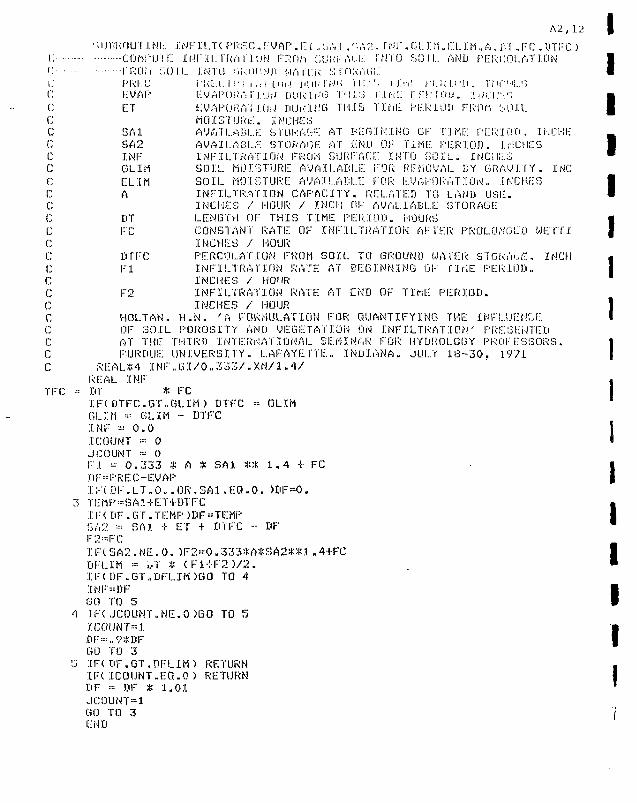
A2,12 I' i U OR 0 U TIN E IN!;:" 11... T ( P R E 0. E V A P. E T ., S, •.! .'•'• A 7 . r N F. G I... I n. E LIM .. A .. D T . F C . 0 T F C )

C COMPUTE INFILTRATION FROh SURi-A'. E INTO SOIL. AND PERCOLATION I': iROii S O I L INTO :.kiiiiND W A U K srnuAiiE II.: P R F C i ' R L l . I ;• i i ,: i J.i.i|J i i ! i | . : I •(••!'•! i l i . i ' ; T i n ! l'l..i.: l.i U i . . TilC'- 1!... 1-'!

C E V A P E V A P O R A T I O N m.iRIi'G TH.!.::; Tin!-: I " F !•: I 'OlJ,. 1 r.'i.:i I'-; mC ET LVAPORA I j.Oi! DUKlfJB THIS TIME PERIOD FROfi bOIL |C MOISTURE. INCHESC SAI AVAILABLE STORAGE AT BEGINING OF TIME PERIOD. INCHE _C BA2 AVAILABLE STORAGE AT END OF TIME PERIOD. INCHES IC INF INFILTRATION FROM SURFACE INTO SOIL... INCHES "C GLIM SOIL MOISTURE AVAILABLE FOR RE-MOVAL BY GRAVITY. INCC ELIM SOIL MOISTURE AVAILABLE FOR EVAPORATION. INCHES IC A INFILTRATION CAPACITY. RELATED TO LAND USE. 1C INCHES / HOUR / INCH OF AVALIABLE STORAGEC DT LENGTH OF THIS TIME PERIOD. HOURS 1C FC CONSTANT RATE OF INFILTRATION AFTER PROLONGED WETTI |C INCHES / HOURC BTFC PERCOLATION FROM SOIL TO GROUND WATER STGRiV.E. INCH .C Fl INFILTRATION RATE AT BEGINNING OF flriE PERIOD.. IC INCHES / HOURC F2 INFILTRATION RATE AT END OF TIME PERIOD.C INCHES / HOUR 1C I-IOLTAN. H.N. 'A FORMULATION FOR QUANTIFYING THE INFLUENCE IC OF SOIL POROSITY AND VEGETATION ON INFILTRATION' PRESENTEDC AT THE THIRD INTERNATIONAL SEMINAR FOR HYDROLOGY PROFESSORS. IC PURDUE UNIVERSITY. LAFAYETTE. INDIANA. JULY 18-30. 1971 jC REAL*4 INF.GI/O.333/.XN/1.4/

REAL INF ITEC - DT * FC I

:I:F(DTFC.GT,,GLIM) DTFC = GLIMGLIM - GLIM - DTFCINF ~ 0 . 0ICOUNT = 0JCOUNT = 0F l -•• 0.333 * A *. SAI « 1 . A + FCDF-PFiEC-EVAPIF(DF.LT.0 . .OR.SA1.EQ.0 . )DF=O.

3 TEMPOSA1+ET+DTFC:CF< DF.GT.TEMP IDF =TEMPSA2 == SAI T ET + DTFC - DFF2==FC

II1

II Ft SA2 . NE - 0 . )F2==0.333*A*SA2** 1 .4+FC IDFLIM = i,T * < F l i F 2 ) / 2 . . •IF(DF.GT„DFLIM)G0 TO AINF-DFGO TO 5

4 IF< JCOUNT.NE.OGO TO 5:tCOUNT--l •DF=..9*DF IGO TO 3

'J IF(DF.GT.DFLIM) RETURN -,IF(ICOUNT.EQ.O ) RETURN IBF = DF * 1.01 'JC0UNT---1GO TO 3 /END

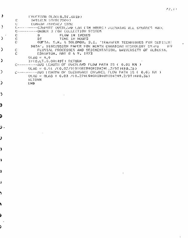
/> 2 , I i

r-'i F U M I N G ALL. SQUARE'1;

C

C

OUilK Q.DT .Giillt >i r! i I:;.G:::R :::TOR< 7500 >COMi-SOO /ASCuE/ STOR

COMPUTE UVERUV-ID LAG (IN HOURS)-ORDER 7> FOR COLLECTION SYSTEMQ FLOW IN INCHESIiT TIME IN. HOURSGUPTA. S.K. 5: SOLOMON- S.I. 'TRANSFER TECHNIQUES FOR GEI) i;^

DATA'. IHSCUSSIOM RARER FOR NINTH CANADIArJ IIYDI'iOLOGY CYi-.RUFLUVIAL PROCESSES AND SEDIMENTATION. UNIVERSITY OF ALBERTA,EDMONTON. HAY G «. 9. 1973

OI..AG = 4.0IF ( Q. L T . 0,. 0 01 * H T ) R E T UR N

-AVG LENGTH OF OVERLAND FLOW PATH IS ( 0.01 KM )OLAG ••= 0.01 /( 0.027S( «.*GRID*GRin*24^ .2/1)7 )*X0.'56J

-AVG LENGTH OK SECONDARY CHANNEL FLOU PATH IS < 0..03 KM )OI...AO = OLAG i 0.03 /< 0.27*< Q:l:0RIi:i:|cGRIIi*249 .2/DT )**0.36 )RETURNEND

i" u iv. T r o H c i... n c; A 5 ( o . » r.. G R :r. o )L Kl r,!...:U4 kUFi;!:S/O .. Q2?i/ „ JiLOPLVO . 0 5 / . i-fl G i . P / 0 . 224/C - - -COMPUTE CHANNEL LAG ( I N HOURS) FOR ARTIFICIAL C O N i m i O M S

CLARAS-- 4 . 0: i .F(Q.LT.0.00001«DT ) RETURNPEPTH == Q.ZlXi Q;ii24y.:l.6:!:GRlD*GRlH/DT >*!'0..3I..IKEA = 3.7?*< Q*249.16*GRID:f:GRlD/DT ):|::i:0.53 a

WIDTH == AREA / DEPI'l-l IRABXUS == AREA / ( DEPTHiDEPTH !-W IDTH )W.L ~ 1 .49/0.025.i:< RA»IUS:!:*.6666667 )TLAGAS ~ GRIIWEI.UETURNf.UO

/\2, U I

II

IIIIIIIIIIII!

'-?,.!:

FUNCTION CLAGNS< Ö.DT.GRID )c roiii'ijTi::: c 11 /• » > i * ; i i.,-.r. ( I N HOURS) ÏOR MATINAL CONBITIONS<: Ü r• i.1 :• -j i H i iJÜII I ISr: n i i .;>,:. h! 1 iuu!-:si- ( . i i i r in. Ü.V-. •:• v;i)i.Hiii:i;-j. s.x. ''WÀ^KJTVM vi::i;iiwiuui.::i I :OR s t j i i . i i ' ^c ur-i i i ' i ' . vi:i.ii(;u>i!:,:tOH I-APKR FOR N.urm C:AMAI.UI.I,' IIYÜROI.noy ; ;;vni'nsjc fT..ui.Mi,M... i:'Uoci:ssi£S AND S E D I M E N T A T I O N . i.w:i:yuiSTTY or A I . ^ E R T A .C ECirilJClTDN. MAY Ö f. 9. 197.6

CLAGNÛ- 10 .00IF( Q. LT. 0 -O0OO1 ;|.'DT ) RETURNC:i.AGNS=GRI.D/( 0.27«( Q*249.16*6RID*GRID/DT )**0.36 )RETURNEND

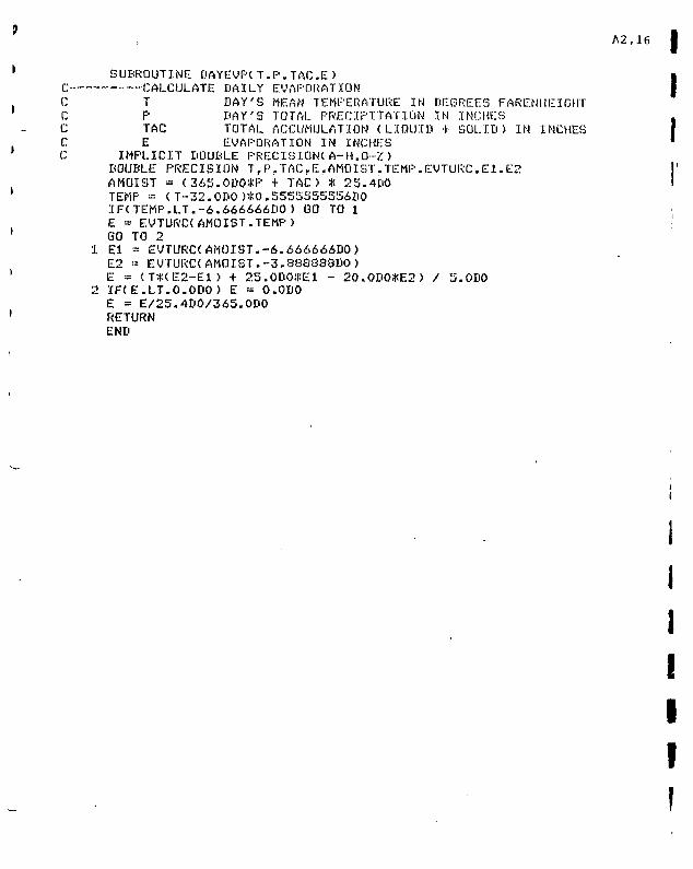
A2,16

UBROUTINE DAYEVPCT.P.TAC.E>C CALCULATE DAILY EVAPORATION IC T DAY'S MEAN TEMPERATURE IN DEGREES FARENHEIGHTC P DAY'S TOTAL PRECIPITATION IN INCHES .C TAC TOTAL ACCUMULATION (LIQUID •»• SOLID) IN INCHES IC E EVAPORATION IN INCHES 'C IMPLICIT DOUBLE PRECISION*A-H.O-Z>

DOUBLE PRECISION TrP.TAC.E.AM0IST.TEMP.EVTURC,El.E2 j'AMOIST = <365.0D0*P + TAC) * 25.4D0 ITEMP •-- (T-32.0D0)*0.5555555556D0IF<TEMP.LT.-6.666666D0) GO TO 1E = EVTURC(AMOIST.TEMP)GO TO 2

1 El -- EVTURC(AM0IST.-6.666666D0>E2 = EVTURC(AM0IST.-3.888888D0)E = tT*(E2-Ei) + 25.0D0«El - 20.0DO#E2> / 5.0D0

2 IF(E.LT-O.ODO) E = O.ODOE = E/25.4D0/365.0D0RETURNEND

II

I

r

'

1

DOUBLE PRECISION FUNCTION EMTURC(P.T)C CALCULATE ANNUAL EVAPORATION USINU TURC'S FORMULAC P ANNUAL PRECIPITATION IN MM .C T MEAN AIR TEMPERATURE IN DEGREES CENTIUKATEC GRAY. D.M.. MC KAY. G.A. AND WIGHAM. J-N. 'ENERGY. EVAPORATIQC AND EVAPOTRANSPIRATION'. IN GRAY. CM- <ED.) 'HANDBOOK OF TliEC PRINCIPLES OF HYDROLOGY'. SECRETARIATE. CANADIAN NATIONALC COMMITTEE FOR THE INTERNATIONAL HYDROLOGICAL DECADE. NO. 8C BUILDING. CARLING AVE. . OTTAWA 1. CANADA (1970).

DOUBLE PRECISION P.TfF.GF = 300.ODO + (25.0D0+0.05D0*T*T)*TF = P / FG == F * F

C MODIFICATION TO TURC'S FORMULA...IF(G.LT.0.1D0) G = 0.1D0

CEVTURC = P / DSQRTC0.9D0+G)RETURNEND

APPENDIX 3

CODE FOR TIME SERIES ANALYSIS ANDSYNTHESIS

A "' MO i'LOG

CA r, CONVERTS MONTHLY FLOW IN CFE

Z TO 'MONTHLY FLOWS IN LOG EASE 10 CFCC

A INTEGER IFILE(IO). JFILE(IO), ISTA(4)9 UCi'iL G< 1 2 )

cft C GET I/O FILES9 TYPE ' INPUT FILE - '

R:ZAD< 11,1000) IF ILErt TYPE 'OUTPUT FILE -'W REAIK 11,1000) JFILE

CALL t)PEN'C20. IFILE. 1. IER )» CALL 0PEN<21. JFILE. 1, IER )

C READ A RECORDv :!.<) r;:EAn<20,1100,END = 900) ISTA. IYR, (0(I). I = 1, 12), AMAX

C CONVERT TO LOGSv 00 20 I = 1. 12* 20 Q< I ) = AL0G10C 0(I ) >

Art AX -• ALOG(IO)

ft C' C WRITE A RECCRP

WRITEC21.2000) ISTA. IYR, (0(1). 1 = 1 . 12), AMAXk GO TO 10

C. C: TERMINATION

-^ 900 CALL RESET' STOP

CA C FORMAT STATEMENTS

1000 FORMAT<10A2)1100 F0RMATC3A2.A1.I3.6F9.2/10X.6F9.2.F10.2)

A 2000 FORMAT*1X.3A2.A1.I3.6F9.6/11X.6F9.6.F10.6)^ END

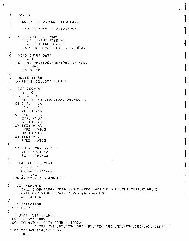
A.i ,

• \M-.

. • i

UA!

tu\r<

, •.,

• i i...

EC-iX)ft... L

[.•:r:.s

• v - >

UT f' INf( 1 1 .

ANNMAL

' ( ~>C< 1

FILENAME:>'JT FILE, 1000 ) IF

C)PEN<20. IF

FLOW

'"TAY(

ILEILE.

DATA

70 )

1 . I

C READ INPUT DATA

.1.0 ;r-:EAI>: 30,1100,END=100 ) AHAX< N )f! -= NflOH:; TO :LO

'C-C WRITE TITLE

100 WRITE< 12.2000 ) IFILECC GET SEGMENT

I ~ 0•J05 I = I M

OD TO C101.102.103.104.900) I101 IYR1 •- 1A

IYR2 " 4100 TO 110

102 IYR1 == 42IYR2 =*57GO TO 110

103 IYR1 = 5E!IYR2 = N+1300 TO 110

104 IYR1 = 14XYR2 = K-113

C110 ND = IYR2-IYR1+1

:;::i. = I Y R I - 1 312 = IYR2-13

cC TRANSFER SEGMENT '

.: == 11-1»0 120 II=1.NDJ ~: J Jc 1

120 ARRAY(II) - AMAX(J)CC GET MOMENTS

CALL CMOM<ARRAY.TOTAL.XB,SD.WAX.VMIN.CM3.CS.CH4,CURT,CVAR,ND)U.:;:ITE( 12.2100) IYRl,IYR2.XB.SDrC£.CURTGC TO 105

cG TERMINATION

900 STOP'CC FC3HAT STATEMENTS

:i.000 FOR«AT< 10fi2 )".000 FrORHAT( ' 1 DATA FROM ' . 1 0 A 2 /

* ' YR1 Y R 2 ' . 3 X . ' X B ( L 0 G ) ' . 8 X . ' S D ( L 0 G ) ' , 3 X . ' C S ( L 0 G ) ' , 6 X . ' C U R T < '2100 F O R M A K 2 I 4 . 4 F 1 5 . 5 )

111

A3, 1

r;

^ :' CC?:; :JTES FIRST ORDER RESIDU.'.LS

INTEGER Ir I!.E* 10 >. JFILE* 10 )

a :,; f !:Gi;::k IYR; 70 ).ir-TA< -t >W :'<;:AL 0< 12.70 >.AMAX( 70 ).C)B( 12 ).QSD( 12 )

Q. C GET I/O FILES*' TYPE 'INPUT FILE -'

READ*11.1000 ) IFILETYPE 'OUTPUT FILE -'

w RCMK 11.1000) JFILEC/iLL OPEN* 20. IFILE. 1, IER )CA-.!_ OPEN* 21.JFILE,2,IER)

C GET SAHPLE PERIODACCEPT 'SAMPLE PERIOD - '.NMON

CC READ DATA

f'Ji - 110 KEftD*20.1100,END = 15 ) I3TA,IYR<ND ),* CU I,ND).1 = 1.12>

DO TO 1015 NH = MD-1

CC FILL. GAPS

HO 20 N=1.NDDO 21 1=0,11,NMONQMiVX = 0.0DO 22 J=1,NKONIF'.Qi IW.M ).GT.QMAX ) QMAX=O( I+J.N)

22 CONTINUE:.00 23 J=1.NMON

23 D( IiJ.N) = GMAX21 CONTINUE20 CONTINUE

f;C FIND AVERAGES AND STD DEVIATIONS

CO 100 1=1.12SUM = 0.0BSO = 0 . 0»D 110 J=1,NDCUM = SUM+GK I.J)

110 SGQ = SSGT!3<I,J)*Q<I,J)

f!B( x ) = SUM/ND:l 00 Q3D( I ) = SQRTC ( SSQ/ND-( SUM/ND >«2 )/( NH-1 ) )

CC FIND FIRST-ORDER RESIDUALS

I>D 200 J=1,ND00 200 1=1,12

200 CK I. J > = GK I. J >-G)B< I )r

C WRITE RESULTS. I ~: — 1WRITE*21.2000) ISTA,J,(QB(I ),I=1,12)J -• 0Ur;ITE< 21,2000 > ISTA , J . ( QSIK I ). I = 1. 12 )i.'Ci 300 J = 1.ND

A3,-1

; r , o o i-.;r?CTC< 2 1 . 2 0 0 0 > I S T A . I Y R C J ) . C CK I . J.". i o r -

r •"•:••:; I . ^ I T ':••]

! vi.n"- I i i i i c i r i T v :! On?, t

! ..(••.• : ;:;.-i1,*iT( 3A2.A.I.. i ; j ,6F9 ..i/10X , 6F9.6 ).'.>,...•. ;•• o: •;••„". /< 1X . .M".2 . i ' i l . 1 3 . 6 F ? . 6 / 1 I X . 6 F 9 .

1IIIIIIIIIIIIIIII

O

COMPILER DOUBLE PRECISIONC SOiUu'.Rr „. ...

"• FIND 3 EC ONE ORDER RESIDUALS FORH rtCK-'THLY FLOWS

KJTZGER IYR< - 1 : 7 0 >,ISTA< 4 )INTEGER 1FILEC.10 ) . JFILE< 10 >:V;::AL a< I . 2 . - I : 7 O > . G C < IOOO.ARRAYC IOOO) ,QCC( IOOO>COHMOH 0.rjQUI VALENCE ( Q( 1 , 1 ) . QC< 1 ) >

cC GET I/O FILES

TYPE 'INPUT FILE -'REAIK 11,1000 ) IFILETYPE 'OUTPUT FILE -•'REAIK 11,1000 ) JFILECALL 0PENC20.IFILE.l.IER)CALL 0PENC21.JFILE.2.IER)

CC GET SAMPLING PERIOD

ACCEPT 'SAMPLING PERIOD - '.NMOH

C READ DATAf.!D = -1

10 Ri£AD(20,1100.END=15) ISTA, IYR( ND ),( 0( I ,ND ), 1 = 1,12 )I!D "«' NH-rlDO TO 10

l5 ND = Ni:i-1NN = 12«ND

CC COMPRESS RECORDS

HO 20 I=1,NN.NMONj - J-M

20 QCC< J ) = QC(I )NN = NN/NMON-1

CC FIND REOUIRED SUMS

GX = 0 - 0SXX = 0 . 03X1 = 0 . 0SXX1 = 0 . 0CXIXI = 0.0PO 100 I=1.KNSX = SX+QCCC I )SXX = SXX+GCCCI )*QCC( I)3X1 = SX1+QCC(1+1)GXX1 = SXXl+GCC(I)*QCC(I+i)

ioo sxixi = sxixi+acc<i+i>*Qcc(i+i)TYPE SX.SXX.SX1,SXX1,SX1X1,NN

C FIND R FISCHER Z-TRANSFORM AND STD ERR* - R = (( SXX1/NH )-( SX/NK )*< SX1/NN ))/( saRT( < SXX/NN )-( SX/NN )*( SX/NN ))

* :i:SQRT( ( SX1X1/NN )-< SX1/WN );i:< SX1/NN ) > )•> ZR = 0 . 5*ALOGt C 1.0+R )/( 1.0-R ) )' r;ZR = SQRT< l.O/C NN+1 ))

TYPE 'H-- '.R.' ZR='.ZR.' EZR=' ,EZR

A i , (, |

f:C Flf.'D SECOND ORDER RESIDUALS j

: W •••-•• N N + 1 • 1

SCC! 1 ) = 0 . 0i'j 2 0 0 1-2. . NM I

:.:00 OCC( I ) - GCCA I )-R*GCC( 1-1 ') I

rC FINI: HOMENTS OF 2ND ORDER RESIDUALS

no 210 i=i.NN..M.0 rtRRAY( I ) = QCC( I >

CALL C«OM( ARRAY.TOTAL.XE,SDEV.VMAX.VMIM.CM3.C3.CMA,CURT.CV,NN>

C: FIM'J 3TB ERR OF 2ND ORDER RESIDUALSZSI" = SDEV/(2.0*NN>

CC EXPAND RECORD

HO 230 I=O..NNK = MMOM*IDO 230 J=1.NMONQCCK+J ) = QCC<1 + 1 )

230 CONTINUECC WRITE RESULTS

WRITER 2 1 . 2 0 0 0 > ISTA, IYR(-1 ).< 0 ( I . - l )»I = 1 .12 ),R.XE,3EEV.CS.CURTWr<ITE< 2 1 . 2 0 0 0 ) ID7A.IYRC0).<Q< 1,0 3.1 = 1.12 J.ZR.EZR.ESD ' IDO 300 J=1.ND I

300 UIRITE< 2 1 . 2 1 0 0 ) ISTA, IYR( J ) . ( Q< I , J ) , 1 = 1,12 >CALL RESET |STOP I

rV.-

C FORMAT STATEMENTS _.1000 FOR«AT< 10A2) I

END

! •

IIII

:.1OO2000 FORMA'H I X . S A 2 . A l . 1 3 . 6 F ? • 6 / 1 I X . 6 F 9 . 6 / 1 1 X . 6 F 9 . 6 )2100 FQRMAT< 1 X . 3 A 2 , A 1 . I 3 , 6 F < ? , 4 / 1 1 X , A F 9 . 6 ) I

III

FLCOJ

cc

GENERATES FLOW VALUES

INTEGER INDEXC100)INTEGER IFILEC 10 >, JFILEC 10 ).NR< 15 ).IOREC< 4000)i;i:AL QC< 20 ).QB( 12 >,RNC 2000 ).RP( 14 ).S3i.i( 12 >.(5BB< '1REAL FHAX< 100 ).FMIN(100 ),P(100 ).PEC 100,15 )

co;mow IORECEKUIVALENCE < IOREC<1 ),RN(1))

GET INPUT DATATYPE 'STATISTICS FILE - ':<F.AT>( 11. 1000 )IFILETYPE 'CRITICAL FLOW FILE - 'i-:.:AlK i 1.1000 )JFILEACCEPT 'INPUT SAMPLE PERIOD - '.NPERACCEPT 'NUMBER OF YRS (1000S) •- ',NYRACCEPT 'YEARS BETWEEN PARAMETER CHANGES - ',MYRACCEPT 'NUMBER OF RUNS - '.NSETACCEPT 'SORT ONLY 0-NO. 1-YES - '.ISRTCALL RESETNV'AL = 12/NPERNRR ~ NYR4NVAL/2f'.VAL = NVAL+2WR1TE( 1 2 , 1 9 9 9 ) NPER.NYR,MYR,NSET,NVftl.,NGR,MVAL

CALL IMIT( 'MTO' ,O, IER>CALL 0 P E N < 2 0 . 1 F I L E . l . I E R )CALL OPEKK 2 1 . J F I L E . 1 , I E R )CALL MTOPIK 2 2 . ' i ' i T 0 : 0 ' , O . I E R )CALL D P E N ( 2 3 . ' F L E R R S ' , 0 . I E R )CALL OPEKK 2 4 . 'RANDRIC , 1 . IER )CALL OPEN(25. 'SYNFLOW',0 , IER)CALL OPEN< 26 , 'RANDPAR' ,0 , IER )

REAIK 2 1 , 1 1 0 0 ) NCRRCADC 2 1 . 1 2 0 0 ) < QC< I ) , 1 = 1,NCR)REABC20,1300) <QB<I ) . 1 = 1 ,12 ) ,R.XS,SDREAIK 2 0 - 1 3 0 0 ) ( GS.CK I ) . 1 = 1 . 1 2 ).ZR.EZR,ESD

SKIP TO SORTIFCISRT.EQ.

IF REQUESTED1 )G0 TO 999

DO 10 1 = 1 . WALQBiI ) = 0B(NPER*I)

10OBB( I ) =GEIK I ) =CR = RCuD » SD

QB< I )DSD<NPER*I

1 2 . 2 0 0 0 ) (OB*I ) . I = 1,NVAL)u'raTE< 12,2001) <QSD< i ) . I = I . N V A L )WRXTE<12.2002 ) R.ZR,EZR.SB,ESByr,:]'TE( 1 2 . 2 1 0 0 ) < I.QC< I ) , 1 = 1.NCR)JO 20 I=i .NCRQC< I ) = AL0P10CQC<I))WRITE'. 1 2 . 2 1 0 5 ) < I . O C d ) . 1=1.NCR)WMTE( 1 2 , 2 2 0 0 ) NYR,< 1.1 = 1 . 1 5 )

A3 ,

GENERATE S Y N T H i i T I CMTTV!"1

;iOXT1

r r- r-

i YRUi'iAQfiS.UO

201 MR<F I R

- o200 I= 0.0

.=: 0=- 0

X == 0

N = .1201 II ) ••••

-= 0 .

BET»:I. ,NE

. 0

.OE+70=1.NCR00

: FLOWS

220 CONTINUECC CONVERT TO LOG OF FLOWS

DO 230 1=1.2000I3E = ]

r . -CISE.EQ. l ) AMAX=0.0fiiX = RN< I >FIR - CR*FIRiSEC*CSBXQ = OBC ISE M-FIR

FIND ANNUAL MAXIF(XO.GT.AMAX ) AMAX=XGIFd3E.LT.NyAL) GO TO 230

IIIIIGET NEXT RN GROUP - SKIP TO NEXT TAPE FILE IF RED'D

DO 210 IG=1.NGRIF'. ITP.NE.500) GO TO 202I if =- 0 •MT - MT+1 |CALL MTDIO<22.30000K.IOREC,ISTAT,IER,NWRDS )WRITEC23.2400) MT.ITP.ISTAT.IER.NURDS _

2 ITP = ITP+1 ICALL MTDIOC22,0,IOREC,ISTAT,IER.NURDS) •WKITEC 23.2400 ) MT.ITP.ISTAT.IER,NWRDSI 'FdER.NE. l ) READ EINARY( 26 )RN I

CONVERT TO NORMALSDO 220 1=1,2000.2 mFAC1 = SQRTC-2.O*ALOG( RN<I )) ) |f:AC2 = 6.2S31853*RN( 1 + 1 )RNd ) = FAC1*COS(FAC2> .RNC1 + 1 ) = FAC1*SIN<FAC2) I

IIF( ISE.GT.NVAL) ISE==1 •

II

FIND POSITION FOR ANNUAL MAX IIIF( AMAX.GT.O.MAX « QMAX=AMAXIF< AMAX.I.T.QMIN ) Qi«N=AMAXJ = NCRi l MHO 240 JJ = 1.NCR IIJ = J - lIF(AMAX.LE.QC<J)> 60 TO 250MR<J> = NR<J)+1

MO CONTINUE I!REVISE TIME SERIES PARAMETER IF REQUIRED ("

250 IYR -•• IYR-UIFdYR.LT.MYR) GO TO 230

A V

• ( ; •

KINAKYC 24 ) ( IVP< I P ) . IP--1 .MVAL )•] 1 P : • 1 . NVfil...' ) ••-•• H ; : ^ •>• J + R P C IF>-uQv>r.!< I P )

. :;•• = c :r-i.o )/< z+i.o >DPI' = 3Di-RP( MVAL )*ESD

C230 CONTINUE

C2:1.0 CONTINUE:

A WSITEC12.2300) ISET,QMAX,( NR<I>.1 = 1,NCR ).QMINv WRITEt 2 5 , 2 3 0 0 ) ISET.GHAX.(NR(I ) . 1 = 1.NCR ),QMIN

200 CONTINUE

w ??? CALL CLOSE(22,1ER)CALL fti_SE< 'HTO' . IER)

® C SORT RESULTSR[::w:i:r«i 25

• DO 300 N=1.NSETRE ADC 25.1400 > FMAX( N ).( NR( I ) f 1 = 1, NCR ).Fi-iIN(N )

A DO 310 1=1.NCRV 310 PE(N.I) = <Nfi:( I )/XN >*100.

300 CONTINUEa CALL £HL1R<NSET,FMAX,INDEX)

DO 320 1=1.NCRDO 330 N=1,NSET

O 330 PC N) •= PEC N.I )V CALL SHL1RCNSET.P.INDEX)

no 340 W=1.NSETA 340 PEC N.I ) = PCN)

320 CONTINUECALL 3HL1RCNSET,FMIN,INDEX)

C PRINT SORTED RESULTSWRITE? 12.2500) NYR,<I,1=1.15)

A DO 350 N=1.N5ET3S0 WRITEC12,2600) N,FHAX(N ).( F'K N,I),1 = 1.NCR),FMINCH>

STOP• f

C FORMAT STATEMENTS1000 FORHAT(10A2)

A 1100 FORMATC 14):;.2OO F 0 R M M T < 3 F 8 . 0 >1300 FORMATC10X,6F9.6 )

A ?y,00 FDRMAT<3X.F10.0.15I6,F?.0>C199? FORMATC'1FL0W GENERATION'//

r * ' INPUT SAMPLE PERIOD (MONTHS) -',110/* ' NUMBER OF YRS ClOOOS', PER RUN -',110/a ' YEARS BETWEEN PARAMETER CHANGES -'.110/

(Q * ' NUMBER OF RUNS -',110/* 'ONUMBER OF VALUES PER YEAR' -',110/* ' NUMBER OF RN GROUPS OF 2000 REOD PER RUN -'.110/

Ai ,10 I

EN Ei

I

:|: ' MUMPER OF fiODEL PARAMETERS - ' . 1 1 0 ) m' 0 0 0 FORMATk ' 0 SEASONAL MEANS : ' . 1 2 F 1 0 . 6 ) I.Mi01 l"0i<nAT< ' 0 STD ERRORS s ' . 1 2 F 1 0 . A )•.002 FORi- iAK ' 0 R s ' .t-9.6*' : ' --TRANSFORM : ' . F 9 . 6 . ' 5 T D ERR ;; ' . F 9 . 6 /

:i ' SD s '.F9.6.' E/JT! ERR j ' . F 9 . 6 ).?:l.00 FORMAK '0 CRITICAL FLOWS s '/( I5.F10.0.15.F10.0.15.F 10.0 ) )::.!.O5 rt.iRMATk'0 LOG CRITICAL FLOWS : '/( I5.F1O.5.I5.F1O.5.15.F10.5 ) ):200 FORMAT( 'O'.TSO. 'CRITICAL FLOW EXCEEDANCE3 IN',I4.-' THOUSAND YRS'/ •

*' SET',2X,'MAX FLOW, 1516.' MIN FLOW/) I'300 FORMAT(I4.F10.0,1516,F9.0>!400 FORnAT(lXr5t8) •;.:'.:J00 FORMATC 'C.T30.'PROBABILITY OF CRITICAL FLOW EXCEEDANCES IN', |

* 14.' THOUSAND YRS (PER CENT)'/* ' P0S'.2X,'MAX FLOW. 1517,' MIN FLOW/) .

2600 FORMAKI4.F10.0,15F7.3.F9.0 ) I

IIIIII

IInIJ

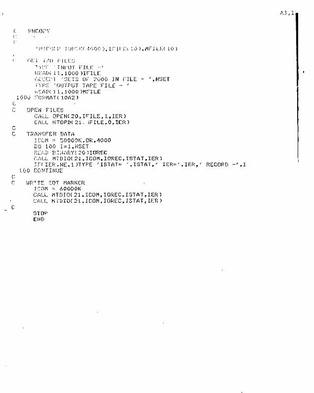
A 3 , l «

(••Ncorv

i f j r o M ' : r.op:::t":( -T>OO >, in\.x:.\ :.o > . M I ~ I L E < I O >

>•• i" i i : . :r i / n i - . r i . . . i : : : : ;•' I : T ' I N P U T FII..I-: -•'\<\-:C4)i 1 1 . 1 0 0 0 )IFILi:.'.LCEPT 'GETS OF ?000 IN FILE - ',NS£TT\FE 'OUTPUT TAPE FILE - 'M:;AI:'( 11.1000 )M:~ILE

1000 FOKMAT<10A2)

C OPEN FILESCALL OPEN(20,IFILE,1.IER )CALL HT0PD<21. iFILE.6,IER)

C TRANSFER DATA•:C;:;M - 500OOK.OR.4000BD 100 I=1.NSETREAS BIWARYC2O5IORECCALL MT»IO(21.ICOM.IOREC,ISTAT,IER )IF< IER.NE.1 )TYPE 'ISTAT- '.ISTAT.' IER=',IER.' RECORD -'.I

100 CONTINUECC WRTTE EOT MARKER

ICOM ~ A000OKCALL MTDIO( 21.ICOM.IOREC.ISTAT,IER )CALL MTDIOC 21.ICOM.IOREC,ISTAT,IER )

CSTOPEMU

APPENDIX 4

CODE FOR GENERATION OF NORMALLY DISTRIBUTED

RANDOM NUMBERS

o0 C RNGITN

I

A '• Gf.N! ' R A T E ! ! ( 0 . : ) RANDOM NUMBERSi.

MMU. R< 2000 >A : .'II:GER iciRECt4ooo)* INTEGER ISDt6>,IFILEt 6 )

l.^MCAL BSDt32)a COMMON IORECW axil. VALENCE < R( 1 >. IOREC< 1 ) )

C^ C OPEN TAPE AND SEED FILE9 CALL OPENt20,'BEED4'.1.IER )

CALL OPENt 22,'SEEDS',0,1ER)

w C GET PARAMETERSTYPE '<14>'

- TYPE 'RANDOM NUMBER GENERATION'* ACCEPT 'OUTPUT - 1 FOR FREE FORMAT TAPE. 2 FOR RDOS DISK FILE' . IDEST

TYPE 'OUTPUT FILE -'a REAM 11.1000) IFILE* I Ft II'EST.EQ.l )CALL MTOPM 21. IFILE, 0, IER )

IFvIBEST.EQ.2)CALL OPENt21.IFILE.0.IER)» ACCEPT 'NUMBER OF SETS OF 2000 - ' ,H'3ET* I GET == 2000

ACCEPT 'USE RN3TART ? tO -> NO, 1 -> YES) -',IBm IFCIB.EQ.O)GO TO 10* ACCEPT 'INTEGER TO START CONGRUENTIAL GENERATOR - '.ISTRT1

ACCEPT 'INTEGER TO START SHIFT GENERATOR - '.ISTRT2% CALL RNSTRTtISTRT1.ISTRT2.ISD,BSD)

GO TO 2010 READt 20.1100) ISD

•» READt 20 .1100) BSD* REAM 20,1100)

READt 20.1100) ISri•* REAE<20.1100) BSD

20 WRITEt22.2000) ISDWRHEt 22.2000) BSD

1 TYPE IS ElTYPE BSDPAUSE:

•J CC GENERATE SETS

ICOM = 50000K.OR.4000k DO 1 I-l.NSET

TYPE 'SET NO. - ',!.' OF'.NSETCALL RNUNITtR.ISET.I3D.BSD)

\ I. Ft IDEST . EG. 1 )CALL MTDIOt 2 1 , ICOM. IOREC .ISTAT, IER )IF<IDEST.EG.2) WRITE BINARYt215I0REC

1 CONTINUE» C

WRITE FINAL SEEDSWRITEt22 .2000) NSET

) WRITEt22 ,2000) ISDWRITEt 2 2 . 2 0 0 0 ) BSDICOM = AOOOOK

. TFiIDEST.EO.2) GO TO 30CALL MTDIOt 21,ICOH.IOREC,ISTAT,IER )CALL MTDlOt 21.ICOH.IOREC,ISTAT.IER )

JO

• t : 0 j

ci >F

;1.

ALiTO!

i ' ' : i

Nil

M i

• I M

RESET

T( 1OAT ( 5 UH I X .

?

5112)

74,2

1

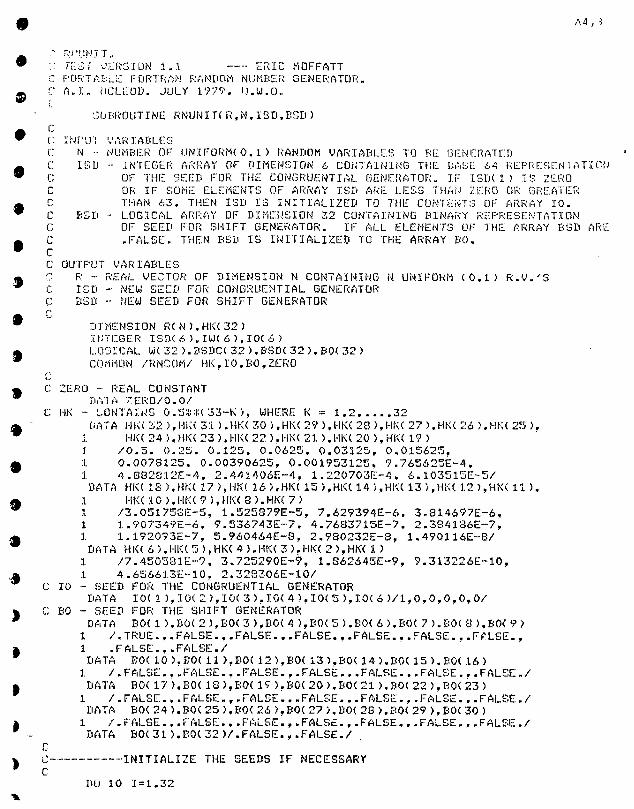
• :: TEST -JERSIQN 1-1 ERIC MOFFATTC PORTABLE FORTRAN RANDOM NUMBER GENERATOR.

^ C A.I. fiCLEOD. JULY 1979. U.W.O.

SUBROUTINE RNUNIT<R,H.1SD.BSD)

w f. I WIT! VARIABLESr; N - NUMBER OF UNIFORM'0.1 ) RANDOM VARIABLES TO BE GENERATED

~ C ISD - INTEGER ARRAY OF DIMENSION 6 CONTAINING THE BASE 64 REPRESENTATION• C OF THE SEED FOR THE CONGRUEiMTIAL GENERATOR. IF IS IK 1 ) IS ZERO

C OR IF SOME ELEMENTS OF ARRAY ISD ARE LEES THAN ZERO OR GREATERm C THAW 63. THEN 13D IS INITIALIZED TO THE CONTENTS OF ARRAY 10.W C BSD - LOGICAL. ARRAY OF DIMENSION 32 CONTAINING BINARY REPRESENTATION

C OF SEED FOR SHIFT GENERATOR. IF ALL ELEMENTS OF THE ARRAY BSD AREm C -FALSE. THEN BSD IS INITIALIZED TO THE ARRAY BO.• C

C OUTPUT VARIABLES- C R - REAL VECTOR OF DIMENSION N CONTAINING N UNIFORM (0.1) R.V.'S• C ISD - NEW SEED FOR CONGRUENTIAL GENERATOR

C BSD -- HEW SEED FOR SHIFT GENERATOR

w ~J IMENSI ON R( N ). Hl<( 32 )INTEGER IED( 6 ).IW(6 ).IOC 6 )

• LOGICAL U( 32 ).3SDC( 32 ),BSD< 32>.B0<32 )9 COCiiiON /RNCCW/ HK , 10,BO,ZERO

/ " •

I..-

C 2ER0 - REAL CONSTANTDATA 7ER0/0 .0 /

C HK - CONTAINS 0 . 5 « < 3 3 - K ) , WHERE K ~ 1.2 32DATA l-ll« 32 ). HK( 31 ). HK( 30 >, HK< 2.9 ) , I-!K( 28 ), HK( 27 ). HK< 26 ). HK< 25 ),

i HK(24). I - IK(23).HI«22),HK(21 ).HK( 20 ), HK( 19)1 / O . 5 . 0 . 2 5 . 0 -125. 0 .0625. 0 .03125, 0.015625,1 0.0073125. 0.00390625, 0.001953125, 9.765625E-4.1 4.882B12E-4, 2 .441406E-4, 1.220703E-4, 6.103515E--5/DATA Hl« IS ),HK< 17 ).HK( 16 ),HK( 15 ).HK( 14 ),HK( 13 ).HK( 12 ).HK( 11 >,

1 HK( 1 0 ) . HK< 9 ). HK( 8 >. HK( 7 )1 /3 .051758E-5 . 1.525879E-5, 7 .629394E-6. 3 .814697E-6.1 1.907349E-6. 9.536743E-7, 4.76S3715E-7. 2 .334136E-7,1 1.192093E-7, 5.960464E-8. 2.980232E-S, 1.490116E-8/

DATA HK< 6 ), HK( 5 ), HKC 4 ). HK< 3 ). HK< 2 ). HK( 1 )1 /7.450581E--9, 3.725290E-9. 1.S62645E-9, 9.313226E-10,1 4.656613E-10. 2.328306E-10/

C 10 - SEED FOR THE CONGRUENTIAL GENERATORDATA I0< 1 ) . I0 ( 2 ) . I 0 ( 3 ) . I 0 < 4 ) . I 0 ( 5 ) . I 0 ( 6 ) / l , 0 . 0 , 0 , 0 , 0 /

C BO - SEED FOR THE SHIFT GENERATORDATA B0( 1 ). B0< 2 ). B0< 3 ), DOC 4 ), E0< 5 >. B0< 6 ). B0( 7 ). B0< 8 ). B0( 9 )

1 / .TRUE. . .FALSE. . .FALSE. . -FALSE. , .FALSE. . .FALSE. . .F^LSE- ,1 .FALSE. . .FALSE. /DATA B0< 10>.B0< 11 ).B0( 12>.B0( 13 ).B0( 14 ).B0( 15).B0( 16)

1 / .FALSE. , .FALSE. . .FALSE. , .FALSE. . .FALSE. , .FALSE. , .FALSE. /DATA B0( 17),B0< 1S).BO( 17 ).B0( 20 >,BOC 21 ).B0( 22 ). BOC 23 )

1 / .FALSE. , .FALSE. , .FALSE. . .FALSE. , .FALSE. . .FALSE. , .FALSE. /DATA B0( 24).BOC 25 ).B0( 24 ).B0< 27/.B0C 2S).B0( 29 ).B0( 30 )

1 / .FALSE. . .FALSE. . .FALSE. . .FALSE. . .FALSE. „ .FALSE. . .FALSE. /DATA B0(31 ) .B0(32) / .FALSE. . .FALSE. /

INITIALIZE THE SEEDS IF NECESSARY

DO 10 1=1.32

IFiESBCI )) GO TO 3010 CONTINUE

CO 20 1=1.3220 :..r:\\i I ? - BCX I )

A4 , 4 1

II

U" ( :•:OIK I > - L T . 0 .OR. I S M I > . O T . 6 3 > G U TO 4 5

:;.;••: ISIK I ).NI:.O> G O TO 60 1

i. A ••\Z, DO 50 I-l.A"50 IS IK I ) = I0( I )

III

II

C- — -—GENERATE H RANDOM NUMBERSC

60 DO 190 IND=1.NCC MULTIPLY BY 6906? USING BASE 64 REPRESENTATION TO AVOID LARGE INTEGERS

I.W( 1 ) - IS IK 1 )*13:i.W< 2 ) = ISD< 2 )*13f ISD( 1 )*55HO 70 1=3.6

70 IW< I) = ISD( I)*13 + ISD( 1-1 )*55+ISD( I-2)*16DO 80 I=1.5 tI U W = IU( I >/64 IIEI.KI) =: I UK I )-IWDV*64I PI = IKLV,-U I PI ) == I UK IP1 HIWDV

BO CONTINUEISB(A) = IUK6)~( IW<6 >/4)*4

Cn OBTAIN BINARY REPRESENTATION

K -• 0

no ioo 1=1,5 1IT = ISD<I> IBO 90 J=1.6

ITT = IT/2 IITTT2 = ITT-MTTBSDC(K) - ITTT2 .NE. ITIT == ITT

90 CONTINUE100 CONTINUE

ES0C<31) = < ISD< 6 )-< ISIK 6 )/2 )*2 > .NE. 0 IBSBC(32) = ISDC6) .OT. 1 »

CC GENERATE A RANDOM INTEGER USING THE SHIFT REGISTER METHOD IC I

DO n o 1=1,17110 BSB< I ) = (BSD(I+15).0R.BSD<I>).AND..N0T.(BSD(I + 15).AND.BSB(I>) i

HO 120 1=18.32 I120 B3IK I > = <BSD< I-17).0R.BSD< I )). AND. .NOT.C BSIK 1-17 ). AND.BSDi I ))

C COMBINE THE OUTPUT OF THE TWO GENERATORS AND CONVERT TO (0,1)DO 170 1=1.32

170 U<I ) = BSDC(I ).AND..NOT.BSIK I) .CR. .NOT.BSDC<I).AND.BSD<I)l\< IMD ) = ZERODO ISO 1=1.32IFC W( I) ) R( IND >=R( IND )+HK( I )

130 CONTINUEC

190 CONTINUERETURNi.MD

I

: PORTABLE FCRTRAN RANDOM NUMBER GENERATOR..: A.I. iiCL.EOI), JULY 1979. U.U.O.

SUBROUTINE RNUNITC R.N.ISD.BSD )

is WU.-:t:,..\- OF UN 11" GRMC 0 .1 ) RANKOH VARIABLES TO BE GENENATIT.liicI.I - JNTLTCR ARRAY or i:iicii-r»:.:iDW & CONTAINING THE EASE <:•'; RFP RE C I T A

OP THE SEED FOR THE CONGRUENT IAL GENERATOR. IF ISDC 1 ) 13 ZEROOR IF SOME ELEMENTS OF ARRAY ISD ARE LESS THAN ZERO PR GREATERTHAN A3. THEM ISO IS INITIALIZED TO THE CONTENTS Or ARRAY 10.

LSD - LOGICAL ARRAY OF DIMENSION 32 CONTAINING BINARY REPRESENTATIONOF SEED FOR SHIFT GENERATOR. IF ALL ELEMENTS OF THE ARRAY BSD.FALSE. THEN BSD IS INITIALIZED TO THE ARRAY BO.

ARE

N UNIFORM ( 0 . 1 ) R.V. 'SOUTPUT VARIABLESR - REAL VECTOR OF DIMENSION N CONTAININGI SI. - r'EW SEED FOR CONGRUENTIAL GENERATORBSD - WZV SEED FOR SHIFT GENERATOR

DIMENSION R(N ).HK(32)I N T E G E R I S I K 6 > , I U ( 6 ) . I O < 6 >LOGICAL WC 32 ).BSDCC 32 5,BSD< 32 ), BO( 32 )

ZERO - REAL CONSTANTDATA ZERC/O.O/

i-iK -- CONTAINS 0 . 5 « ( 3 3 - K > . WHERE K = 1 . 2 , . . . . 3 2DATA HUC 32).HK( 31).HK<30),HK( 29).HK<2B ).KK( 27 ),HK(26 ).HKC23 ),

1 HKC 24 >, HK( 23 ). HK( 22 >. HK( 21 ), 1-1 K( 20 ). HK( 19 >1 / O . 5 . 0 .25 . 0 .125 . 0 .0625, 0 .03125. 0.015625.1 0.0078125. 0.00390(423. 0.001953125. 9.745625E-4,1 4.SG2(312E-4. 2.44140AE-4, 1.220703E--4. 6.103515E-5/DATA HKC IS 5.HK< 3.7 ).HK< 16 >.I-!K( 15 ).HK< 14 ),HK< 13 ).HK( 12 ),HK( 11 >.

1 HKC ::.O >.HK< 9 ).H!« 8 >.HK( 7 )1.525879E-5, 7.629394E-6, 3.814697E-6,

9.536743E-7. 4.7683715E-7, 2.384186E-7,5.960464E-3. 2 .980232E-8. 1.490116E-8/HK< A >.HK( 3 ).HK< 2 ).HK< 1 )

3.725290E-9, 1.862645E-9, 9.313226E-10.2.328306E-10/

10 - SEED FOR THE CONGRUENTIAL GENERATORDATA IOC1 >, I0(2 ) . I0<3 ) . I 0 ( 4 ) . I 0 ( 5 ) . I 0<6 ) / l , 0 , 0 , 0 , 0 . 0 /

BO - SEED FOR THE SHIFT GENERATORDATA BOC 1 ). BOC 2 ). B0< 3 ). BOC 4 ), BOC 5 ).BOC 6 ), BOC 7 ). BOC 3 ). BOC 9 )

1 / .TRUE. , .FALSE. . .FALSE. , .FALSE. . .FALSE. , .FALSE. , .FALSE. ,1 .FALSE. . .FALSE. /

DATA COC 10).BOC 11 ),B0( 12).B0( 13),BOC 14 ).BOC 15 ). BOC 16)1 / .FALSE. . .FALSE. , .FALSE. . .FALSE. . .FALSE. . .FALSE. . .FALSE. /DATA BOC 17).BOC 18).BOC 19 ).BOC 20 ).BOC 21 ).BOC 22 ) . BOC 23 >

1 / .FALSE. , .FALSE. , .FALSE. . -FALSE. , .FALSE. . .FALSE. . .FALSE. /DATA BOC 24 ).BOC 25 ).BOC 26 ),BOC 27 ),BOC 23 ).BOC 29),BOC 30)

1 / .FALSE. . .FALSE. , .FALSE. . .FALSE. . .FALSE. , .FALSE. , .FALSE. /DATA BOC 31 ),BOC 32 ) / .FALSE. . .FALSE. /

1 /3 .051758E-5 ,1 1..907349E-6.1 1.192093E-7,

DATA l-lK( 6 ) . HK< 5 ).1 /7 .450581E-9 ,1 4 .656613E-10.

- INITIALIZE THE SEEDS IF NECESSARY

DO 10 1=1 .32IF(BSDv I ) ) GO TO 30

10

'•'•' .'.••". I.K I ; •• HOC I )

. ' . 0 - f i 4 0 I - 1 . &!.!•"•: I. S I K T ) . L T . 0 . O R . IGI .K I ) . G T . A 3 ) GO T O 4

I

• •.0 :.:Oi.'TlNUE II T i I S D ' 1 5 . N E . O ) GO TO 6 0 I

•v:, :.'.o so 1=1 .650 ISM I > -- I0< I > I

r IC GENERATE N RANDOM NUMBERS

6 0 DO 1 9 0 IND=1,N |

C MULTIPLY BY 6906? USING BASE 64 REPRESENTATION TO AVOID LARGE INTEGERSIWC 1 ) = ISD( 1 ) * 1 3 IX'4\ 2 ) "" ISD( 2 )*K 13"I'ISD( 1 ) $ 5 5 •

7 0 IW( I ) = ISD( I )*13-MSD( 1 - 1 )*55+IStK I - 2 ):lDO 8 0 1 = 1 . 5IWDV = T.U< I ) / 6 41SD< I ) = I UK 1 >-IWIJV*64 |I PI -• I-H §IU( IP1 ) = IUK IP1 )+IWIW

!30 CONTINUEXS1K6) = MOD( IU)C6),4) I

C •C OBTAIN BINARY REPRESENTATION

K ~ 0 1DO 100 1=1.5 IIT = ISD(I)DO 90 J=l,6 |K = K+l IBGDC(K) = .FALSE.ITT = IT/2 m

T.TTT2 == ITT+ITT Ili«ITTT2 .NE. IT) BSDCCK) = .TRUE. . •IT == ITT

r>0 CONTINUE I100 CONTINUE •

BSDCO1 ) = .FALSE.:n-<MDIiCISD<6>.2> .NE. 0) BSDCC 31 ) = .TRUE. |BSDC5 32) = .FALSE. |IFCISIK6) .GT. 1) BSDC(32) = .TRUE.

C GENERATC A RANDOM INTEGER USING THE SHIFT REGISTER METHOD IDO 110 1=1.17

1.1.0 UK I > = BSD< 1+15)DO 120 1=13,32

120 UK I) = .FALSE. 'DO 130 1=1.32

130 UK I) = W<I).AND..NOT.BSD(I) .OR. . NOT.UK I ). AND. BS»( I )DO 140 1=18,32

140 BSD(I) = U<1-17)DO 150 1=1,17

150 BSD<I> = .FALSE.DD 160 1=1.32

1.60 BSDC I ) = BSD( I ).AND. .NOT.UK I ) .OR. .MOT.BSDC I ).AND.W< I )CC COMBINE THE OUTPUT OF THE TWO GENERATORS AND CONVERT TO (O.I) VARIABLE

DO 170 1=1.32

ar-J, IND) -•= ZERO

A 4 , 7 |

7 0 U( I ) = BS3JC< I ).Ac>r.i..N0T.B3D( I ) .OR. .NOT .BSHC( I ) . ANB. E<SD< I >':', IND ) -- ZERO10 1.80 1 = 1 ,,32

n !•;••( WU ) ) R( I.NU ) •••= VV< IND )fHK( X )j ; ; i ) CDKT1NUE

« l ? 0 CONTINUE

»

A4,B

>• ,-,:.ii:i!-;:,M':i' tiuw^-i.M !;•.•;:.: F O R USE: W I T H R B U N I T . R N S T R T C A N W : U S E D ;O co;;v::i-ri:t;:i;(- (:;rr ~i\>.. K::I::K; ISIJ A N D I;-:;D I N R D U N I T .

:.-:.)OliOljTINE RMSTRTv ISTRT1. ISTRT2 . ISD .BSD )CC: INF-tn VARIABLESC :;3TP:T1, ISTRT2 - INTEGERS USED TO SET SEEDS ISD AND BSDC:C OUTF'UT VARIABLESC ISD - ARRAY OF DIMENSION 6 CONTAINING THE BASE 64 REPRESENTATIONC OF ISTRT1 OR ISTRT1 + 1 ( ACCORMNG A3 I3TRT1 IS ODD OR EMEN)C BSD - LOGICAL ARRAY OF DIMENSION 32 CONTAINING THE BASE 64C REPRESENTATION OF ISTRT2 MODULO 2043C

DIMENSION ISIK6)LOGICAL BSD(32):i I = ISTRT1DO 10 1=1.5:::s»i i) = HOIK II,64)II == 11/64

10 CONTINUE:i::ia< 6 ) = MOD< II,4 >I GDC 1 ) -~ ISD( 1 )/2*2+lII ~ MQD(ISTRT2.2049)00 20 1=1 .32BGD<I ) = .TRUE.IF<MOD(11,2) .EQ. 0) BSD<I) = .FALSE.II = 11/2

20 CONTINUERLTURNCND

APPENDIX

LETTER FROM H. G. ACRES TO SECRETARY TREASURER

OF GRAND RIV .P. CONSERVATION

COMMISSION

April 3, 1943.

B.J?. Roberts, Esq., Secretary-Treasurer,Grand River conservation commission,BOX 7 2 0, BHAHTIS'OSD, Ontario.

Dear Mr. Boberta:

Confirming yesterday»a telephone conversation withyou from shand, the peak of the seoond freshet passad throughthe &rani Valley Dan between tho hours of 10 A.M. and 4 2.if.on April 1st . The HOY/ passing through daring this periodwas at the rate of 13,500 second-feet, which is 637. in oxcessof any estimated, and more than double any previously-recordedpeafc flow.

• . The mathematical chance of reonrrence of a peak flowof 13,500 second-feet from the basin above tho Grand Valloy Dam,is less than 1 in 100,000.

Tho maximum elevation reached in Belwood lakB wasI393.5, whloh i s within 6" of the designed maximum storagel l f elevation 1394.

Daring the last 5 days of March 35,509 acre-feet of8 impounded in Belwood Lake. This volume of storage,

g ^ * witb- tho flow which was meanwhile passing through thoDan, i s equivalent to an average inflow of about 4,000 second-feet, during the 5-day period, fron the tributary basin.

At the beginning of the above 5-day period the waterin B9lW°oi l a l t e w a° a t 0 ^ i l l ; 7 a y crest 3avel, so that It api;oar3that Belwood Laia h^a Gofficiont capacity to absorb the v/holeof a nornal pealc x^0** froa the tributary basin.

\7han I was up at aha r^_ja star dag, I gave Cameron in-Ptructions to Jaave the Eatoa at thoirfhca opening unti l tho

Lke 1««1 ^ d ^oppod to nt leant olevation 13g5 anBelwoodJ

1««1p g i to

to nt leant olevation 13g5, and

• • : < & •

A5 , 2

K.21.Roberts,Esq.,Seoy-Troas. - 2. Apr.3/45.

he advised this morning that this drawdown had been reaohod.Ho r;as Instructed to^gradually_clqae the Rates, but to allowthe drawdown to oontin'ae_'td"elev;aTifin_^82^ ponding furtherinstructions. There were 22 degrees of frost at Fergus thisnornii;^, and thare is s t i l l dangor of another heavy riae ifa sudden riao in temperature should be accompanied by a heavyrainfall on the frozen ground.

' In any event the Grand Valley Dam has had a test'whloh i s not likely to be repeated in our time.

Youro very truly,GRAUD HIVBR CONSERVATION CO1DHSSIOH,

H. G. Acres,

Chief EngineerHGA/CL.o-MeB8ra.Philip,Gait.

Pequegnat, Kitchener.Dr.T.H.Hogg,Tor onto(Perao nal)

TABLE

HAIER SURVE* OF CANADA GR^O HIVER NEAS HARSvILLE STÙTtQN NO.AUG i 1979 PAGF 221GUELPH. ONt ANHUAl Exr«E1ES OF DISCHARGE IN CFS AND ANNUAL TOTAL DISCHARGE IN «C-Fr FOR THE PERIOO OF RECORD

»EAR

195039? l1951 J.a.6.195 i IT i

! 19651966196<-196»1969

1970i 197 1

1972197 3

: 197"«~

I 1975' 1976! 1977

MAXIMUM INSTANTANEOUS_0ISCHARGE HAKIHUH D»[LT DISCHARGE

--//f/OO CPS" . . ??J?° ess— 7r9a c/^s-

.**>..**!>£ S_?

5330 CFS AT 1000 EST ON APR 125270 CFS AT 0001 EST ON JAN 17280 CFS AT 01U5 EST ON APR 35950 CFS «T 07.50 EST Ort NO* 295700 CFS ~AT 15 Di. EST ON APR ï é

7210 CFS AT 21«.<i EST ON APR lit7210 CFS AT 1707 EST ON APR IS

1J700 CFS AT e n . 9 ESf ON APR 1»58">0 CFS AT 0301 EST ON HAR_IZ

'6730 CFS AT 1216 EST ON'«PR V

11700 CFS AT 120«. EST ON APR 1911600 CFS AT 0901 EST ON MAR Zi.10300 O'S AT 1908 EST OH MAR 13

7150 CFS_AT O03_Z_EST_ ON APR 13_

HINIMUH (JAIL» DISCHARGE

_11.90l)._CFS_0H.HAR 2071.00 CFS ON HSR 28

B3<«0 CFS OH APR u_ 6<«30 CFS OK H1R_33_

5S20 CFS'ON APR 1

1.790 CFS ON »PR 123170 CFS ON JAN 153ûfl CFS ON APR 3

. 5 1 1 0 CFS 0(1 NDY 29_"•930 CFS ON APR! 5

5693 CFS ON APR 156860 CFS ON APR 139330 CFS ON APR IS5050 CFS ON MAR 126300 CFS ÔH "APR >.

1.0 CFS ON AUG0 CFS ON JUL

S31

1.0 CFS ON AUG 211.0 CFS ON JUL 251.0 tFS ON BUG 27

Ï . 2 CrS ON AUG 255.« CFS UN onr T6.1 . CFS ON JUN 7B.t_CFS ON JUL ZU8.6 CFS ON O C T " > ~

7 .1 CFS OH AUG 27"••1 CFS ON OCT 82 .0 CFS ON SEP 233.5_CFS ON_OCT 12

"6.0 CFS'ÔN SEP 2".

IO800 KFS ON APR 19 1 1 . 1 CFS ON JUN 2710200 CFS ON M»R 21 9 .0 CFS ON JUN 2<<

8 5 7 0 CFS ON HAR 1 3 <•• 8 C F S ON JUN 2<t6 m O C F S ON APR 1 3 16.2 CF5 ON SEP 9

. TOTAL. DISCHARGE

196000 AC-FÏ199000 AC-FT

207000 AC-F7281.000 AC-FT168000 AC-FT

222C00 AC-Frl".9003 AC-FT322005 AC-FT

__ 239000 AC-FTJlSobo'AC-FT

169000 AC-FT1S3000 AC-FT

tC-FT

AC-Fr

182G0O AC-FT23J000 »C-FT2I6C00 AC-FT187000 AC-FT

TEAR

I9t819U9

195019511S52

196519&61967

197019711T7 213731371.

1975197619771 9 7 B

- EXTREME RECORDEO FOR THE PERIOO OF RECORD 206030 AC-FT HE AN

"Note : " TheTbäsTn "of" the" Grand" RÏver' near ^ r s v i ï ï e is about 8£'the basin drained by the Grand River at the Shand Dam

the size