Approved:

THE DEVELOPMENT OF

A DIGITAL DATA PROCESSING SYSTEM

FOR TWO-PHASE TURBULENCE DATA

by

Sung Jin Lee

A Thesis Submitted to the G raduate

Faculty of Rensselaer Polytechnic 1 nstitute

in Partial Fulfillment of the

Requirements for the Degree of

MASTER OF SCIENCE

~ PrOOrô: ê. Jones, Jr. Thesis Co-Advisor

Rensselaer Polytechnic 1 nstitute Troy, New York

December 1982

_.,.,.··

· ..

CONTENTS

page LIST OF TABLES . . . . . . . . . . . . . . . . . . . . . . . . . . . . . . . . . . . . . . . . iv

LIST OF FIGURES . . . . . . . . . . . . . . . . . . . . . . . . . . . . . . . . . . . . . . . v

NOMECLATURE . . . . . . . . . . . . . . . . . . . . . . . . . . . . . . . . . . . . . . . . . . . vii

ACKNOWLEDGEMENT . . . . . . . . . . . . . . . . . . . . . . . . . . . . . . . . . . . . . . . ix

ABSTRACT . . . . . . . . . . . . . . . . . . . . . . . . . . . . . . . . . . . . . . . . . . . . . . x

1. INTRODUCTION 1

2. EXPERIMENTAL APPARATUS AND DATA ACQUISITION SYSTEM . 4

Air/Water Loop ........................ ·. . . . . . . . . . . 4 Hot Film Anemometry. .. . . . . . . . . . . . . . .. . .. .. . . .. . . . 6 Signal Conditioning. .. . . . .. . . . . . . . . . . . . . .. .. . . . . . 9 Data Acquisition System .......................... 10 Preliminary Calibration of The Anemometer . . . . . . . . 13 Frequency Response of The Anemometer ............. 13 Noise and Accuracy . . . . . . . . . . . . . . . . . . . . . . . . . . . . . . . 16 Simultaneous Digitization ........................ 18

3. PHASE DETERMINATION TECHNIQUE ...................... 21

Anemometer Signal Interpretation ................. 21 Digital Implementation of Phase Determination

Technique . . . . . . . . . . . . . . . . . . . . . . . . . . . . . . . . . . . 27 Description of Computer Codes, VOID1 and VOID3 . . . 28 Re sul ts ........................... ·............... 30

4. DIGITAL COMPUTATION OF FLOW PARAMETERS ............. 31

One Dimensional Data . . . . . . . . . . . . . . . . . . . . . . . . . . . . . 32 Liquid Phase Indicator Function ............. 32 Local Void Fraction ......................... 31 Mean Liquid Phase Velocity .................. 32 The RMS Value of The Liquid Phase Velocity

Fluctuation . . . . . . . . . . . . . . . . . . . . . . . . . . . . 33

Three Dimensional Data ........................... 33 Local Void Fraction ......................... 34 Reynold's Stresses .......................... 34 Anisotropy Factor ........................... 36

5. SPECTRAL ANALYSIS OF DIGITAL DATA .................. 38

ii

,. ! ' 1

: : 1 ,( •• 1

• 1 1 1

1

Auto and Cross-correlation Functions . . . . . . . . . . . . . 39 The Auto correlation Function and The Liquid-phase

Turbulence Scales . . . . . . . . . . . . . . . . . . . . . . . . . . . 40 Power Spectral Density Functions ................. 40 Cross-spectral Density Functions ................. 42 Coherence Function ............................... 43 Computation of Correlation Estirnates . . . . . . . . . . . . . 43 Computation of Power Spectrurn Estirnates . . . . . . . . . . 45 Finite Length Effect ............................. 45 Discrete Tirne Effect ............................. 48 Determination of Digitization Rate ............... 52 Spectral Analysis of Segrnented Signal . . . . . . . . . . . . 53 Description of The Spectral Analysis Code, POWER . 54 Results . . . . . . . . . . . . . . . . . . . . . . . . . . . . . . . . . . . . . . . . . . 57

6. SUMMARY AND CONCLUSIONS ............................ 68

REFERENCES 69

APPENDIX A - THE LIQUID-PHASE TURBULENCE SCALES . . . . . . . 70

APPENDIX B - USING DISCRETE FOURIER TRANSFORM FOR CORRELATION ESTIMATES .................... 74

APPENDIX C - HOW TO READ THE HP PRODUCED MAGNETIC TAPE WITH THE IBM COMPUTER ............... 78

APPENDIX D- COMPUTER PROGRAM LISTING ................. 84

iii

LIST OF TABLES

Page Table I List of Window Functions ................... 49

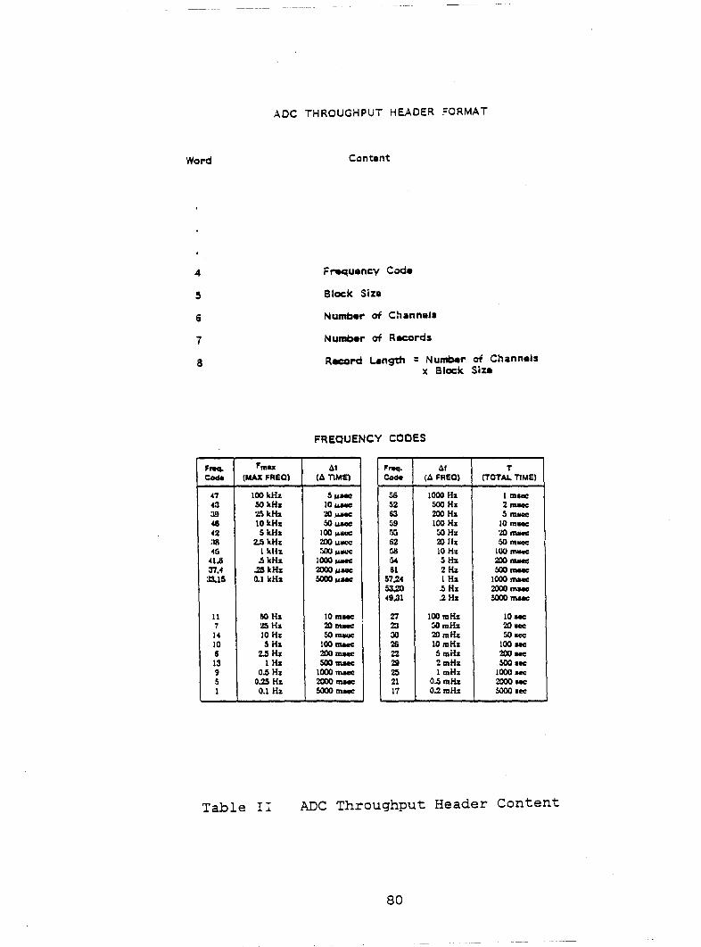
Table II ADC Throughput Header Content . . . . . . . . . . . . . . 80

iv

Figure 2.1

Figure 2.2

Figure 2.3

Figure 2.4

Figure 2.5

Figure 2.6

Figure 2.7

Figure 2.8

Figure 2.9

Figure 3.1

LIST OF FIGURES

Page Schematic of Air/Water Loop.... .. . . . . . .. . . 5

Probe Mounting Fixture 7

Dimensions of The Conical Probe 8

Circuit Diagram of The Clipping Circuit . . . 11

Signal Conditioning of Two-phase Data ..... 12

Schematic of The Data Acquisition System . . 14

Conical Probe Velocity Calibration Data . . . 15

Electrical Testing Result of The Conical Probe . . . . . . . . . . . . . . . . . . . . . . . . . . . . . . . . . . . . . 17

Simultaneous Digitization Result of A Square Wave . . . . . . . . . . . . . . . . . . . . . . . . . . . . . 20

Schematic of Bubble Passage Through A Conical Probe . . . . . . . . . . . . . . . . . . . . . . . . . . . . . 23

Figure 3.2 Modified Schematic of Bubble Passage Through A Conical Probe ................... 26

Figure 3.3 The Digital Signal and The Corresponding Phase Indicator Functions ................. 29

Figure 5.1 Rectangular Window Function and Its Fourier Transform ......................... 47

Figure 5.2 Effect of Discrete Time Sampling On The Fo~rier Tranform of a Signal .............. 51

Figure 5.3 Power Spectrum of The Pseudo Liquid Phase Indicator Function . . . . . . . . . . . . . . . . . . 55

Figure 5.4 Schematic of The Power Spectrum Computation of Two-phase Data ......................... 56

Figure 5.5 Schematic of Computing Correlation and Power Spectrum Estimates .................. 58

Figure 5.6 Autocorrelation of a Sine Function 59

Figure 5.7 Power Spectrum of a Exponential Autocorrelation Function .................. 60

v

i•

Figure 5.8 Cross-spectrum of a Shifted Exponential Cross-correlation Function ................ 62

Figure 5.9 Autocorrelation Function of Single-phase Data . . . . . . . . . . . . . . . . . . . . . . . . . . . . . . . . . . . . . . 63

Figure 5.10 Cross-correlation Function for A Pair of Shifted Single-phase Data .............. 64

Figure 5.11 Power Spectrum of Single-phase Data ....... 65

FigUre 5.12 Power Spectrum of Two-phase Data .......... 66

Figure B.1 4-Point Circular Convolution of Two Sequences 75

Figure C.1 Data Word Content ......................... 81

Figure C.2 Schematic of the Relationship Between The Analog Signal and The Corresponding Digital Representation in The Data Word . . . . . . . . . . . 82

vi

a, ~' o

0 (f) x y

E

E(n)

e(n)

v

U(n)

u

u(n)

v(n)

w(n)

f

f

Rx(•)

R (t} x y

Gx(f)

Gxy(f}

Af

Àf

0 2 x

X(n)

NOMECLATURE

Local Void Fraction

Directional Sensitivities of the Probe Sensors

Coherence Function

Anemometer Output Voltage

Digitized Anemometer Output Data

Fluctuating Components of the Digitized Anemometer Output data

Fluid Velocity

Instantaneous Axial Liquid-phase Velocity

Mean Axial Liquid-phase Velocity

Fluctuating Components of the Axial Liquid-phase Velocity, U(n) = U + u(n)

Radial Liquid-phase Velocity Fluctuation

Azimuthal Liquid-phase Velocity Fluctuation

Time Displacement

Space Displacement

Frequency

The Longitudinal Correlation Coefficient

Autocorrelation Function of x(t)

Cross-correlation Function of x(t) and y(t)

Power Spectral Density Function of x(t)

Cross-spectral Density Function of x(t) and y(t)

The Integral Scale of The Liquid Turbulence

The Dissipation Scale

Variance of x = x 2

Liquid Phase Indicator Function

vii

x+(n)

X(f)

x(rn)

OPERATORS

Pseudo Liquid Phase Indicator Function

Liquid Phase Density

Gas Phase Density

Sarnpling Period

Fourier Transforrn of x(t)

Discrete Tirne Sarnples of x(t) where t=rnT

t Expectation Value, or Vector, or Matrix

VAR Variance Matrix

x(t)*y(t) Convolution of x(t) with y(t)

* X(f) Cornplex Conjugate of X(f)

SUBSCRIPTS

1 1 2 1 3 Of Sensor 1, 2 1 3

2t Of Two-phase flow

UNITS

SCFH Standard Cubic Feet Per Hour

viii

ACKNOWLEDGEMENT

The author wishes to express his gratitude to Drs. R.

T. Lahey, Jr. and O. C. Jones, Jr. for the guidance and

encouragement received under their supervision. The work of

Kong Wang in setting up the experimental apparatus and

making the preliminary calibration runs is acknowledged.

Also the support of the National Science Foundation (Dr. Win

Aung) is gratefully acknowledged.

Finally, the author is especially grateful to his wife,

Young Mae, for her patience and understanding during the

preparation of this manuscript.

ix

ABSTRACT

A digital data acquisition and reduction system to

process two-phase turbulence data from hot film anemometers

were developed and tested against both actual and

hypothetical data. In particular, the interpretation of the

two-phase turbulence signal and the digital technique

developed for phase determination was discussed in detail.

The latter method is based on a cornbination of level and

slope thresholding. It was applied successfully to the phase

determination of actual two-phase data.

The data reduction system can handle digital signals

from either a single-sensor or a three-sensor probe. From

single-sensor data, it computes the local void fraction,

mean axial liquid phase velocity, and the axial liquid phase

turbulence intensity. From three sensor data, it computes

the local void fraction, and all six components of the

Reynolds stress tensor. It also performs spectral analysis

of the data and computes the autocorrelation function, the

cross-correlation function, the power spectral density func­

tion, and the cross-spectral density function.

x

--------------

CHAPTER 1

INTRODUCTION

The local void fraction and the statistics of the phase

velocity of the continuous phase are two of the most

important parameters characterizing a fully developed

two-phase turbulent flow. Although past attempts have been

made with hot film anemometry, no reliable method has been

developed with which to measure these two quantities simul­

taneously. This is particularly true when one is concerned

with three-dimensional velocity fluctuations.

Hot film anemometry consists of a miniature sensing el­

ement attached at, or near, the tip of a supporting probe

and a feedback circuitry. For constant temperature

operation, which is usually prefered over constant current

operation, the sensing element is electrically heated to a

constant temperature, higher than the arnbient f1uid

temperature. The feedback circuit senses any variation of

the sensor temperature due to the convective cooling by the

fluids and tries to restore the sensor temperature by

sending more or less current to the sensor. Hence, the time

history of the current through the sensor can be related to

the f1uid velocity fluctuations at the sensor. In principle,

the three-dimensional instantaneous velocity can also be

measured with this technique by using three sensors in an

1

appropriate configuration.

Liquid cools the sensor more effectively than gas.

Hence when the sensor is immersed in the gas phase much less

current is required to keep the sensor temperature constant

than in liquid phase. This fact can be used when operating

an anemometer in two-phase flow to determine the local in­

stantaneous phase [1] .

The project reported on herein was motivated by the

analytical model Lahey and Drew derived to relate the

lateral void distribution to the liquid phase turbulence

distribution [2] . In order to verify the analytical model,

one needs experimental measurements of the lateral void dis­

tribution as well as the three-dimensional liquid turbulence

structure of a flow through ducts of various geometry. In

order to develop the technique, a cylinderical duct

installed in a two-phase flow loop was used with a

single-sensor TSI hot film probe for one-dimensional

measurements. However, the data acquisition and reduction

system was developed to process signals from both single and

three-sensor probes.

This thesis starts with a brief description of the

airjwater loop and various measurment deviees. Then the

preliminary calibration curve and the frequency response

curve of the anemometer will be discussed. The majority of

the thesis is devoted to a description of the digital data

2

reduction system. In particular, the determination of phase

and spectrum from the digital data is discussed in detail.

3

CHAPTER 2

EXPERIMENTAL APPARATUS AND DATA ACQUISITION SYSTEM

AIR/WATER LOOP

The airjwater loop and arragement of the measurment

deviees are shown in Fig. 2.1 . The water is drawn from the

city water main to give flow rates up to 4 x 10- 4 m3 js. To

vary the water temperature from 55°F to 130°F, hot tap-water

can also be mixed with the feed water. The water passes

through a custom-made orifice flow meter(featuring three

meters of different ranges in prallel) and is routed into

the bottom of the loop.

Two-phase flow is simulated by injecting air through

either an air stone or a mixing tee from the bottom of the

loop. Three parallel rotometers are used to control the air

flow rate from 1 to 100 SCFH. We can achieve virtually any

flow regime of interest in this loop. The two-phase flow

exits via the top of the loop into a water storage tank;

hence, this airjwater loop is a once-through cycle.

The test section is a one-inch diameter plexiglass

pipe. About 60 inches above the bottom of the loop, a TSI

1231 W conical hot-film probe and a pitot tube are mounted

at diametrically opposite sides such that they can traverse

4

TO WATER COLLECTION TANK

U-TUBE MANOMETER

l

CONICAL TO PROBE ANEMOMETER

TWO-PHASE (AIR/WATER)

FLOW

AIR STONE

THERMOCOUPLE

WATER IN LET

~

-HOT WATER

TO THERMOCOUPLE TEMPERATURE

READ OUT

ORIFICE #2

U-TUBE MANOMETER

Figure 2.1 Schematic of AirjWater Loop

5

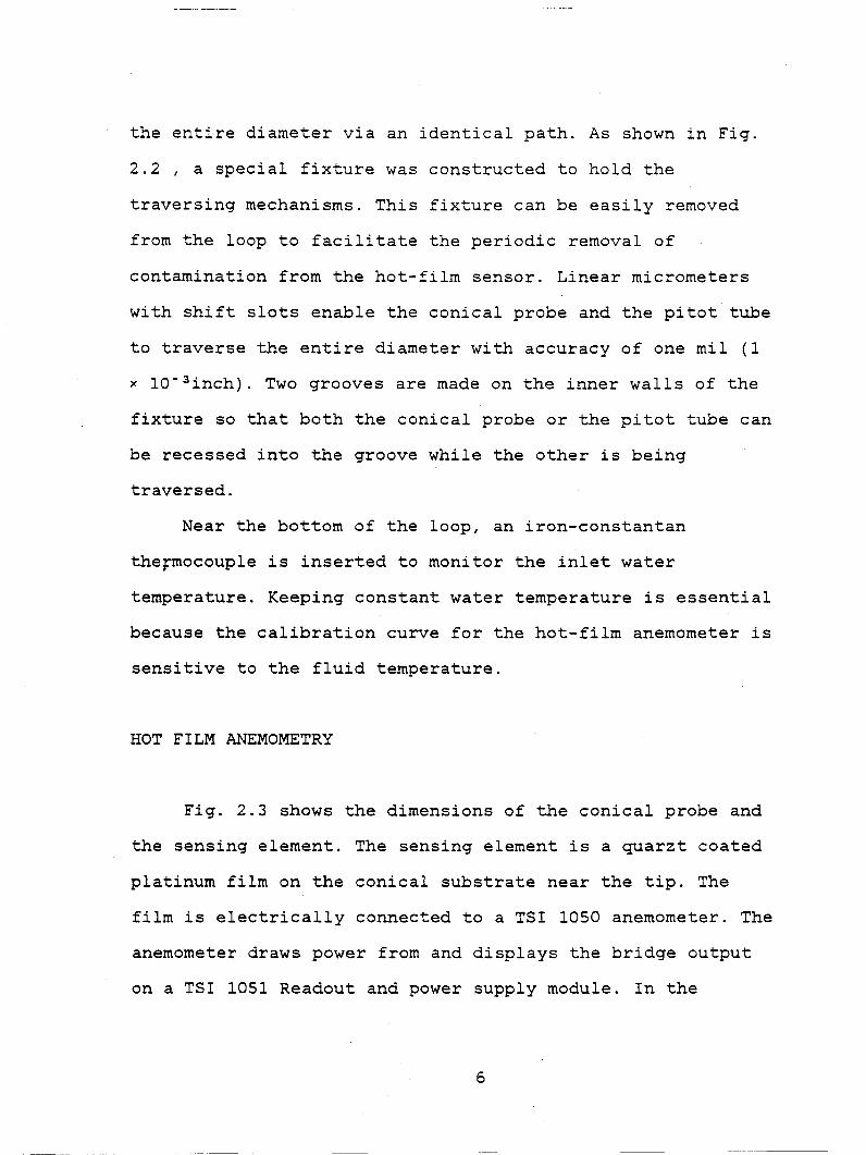
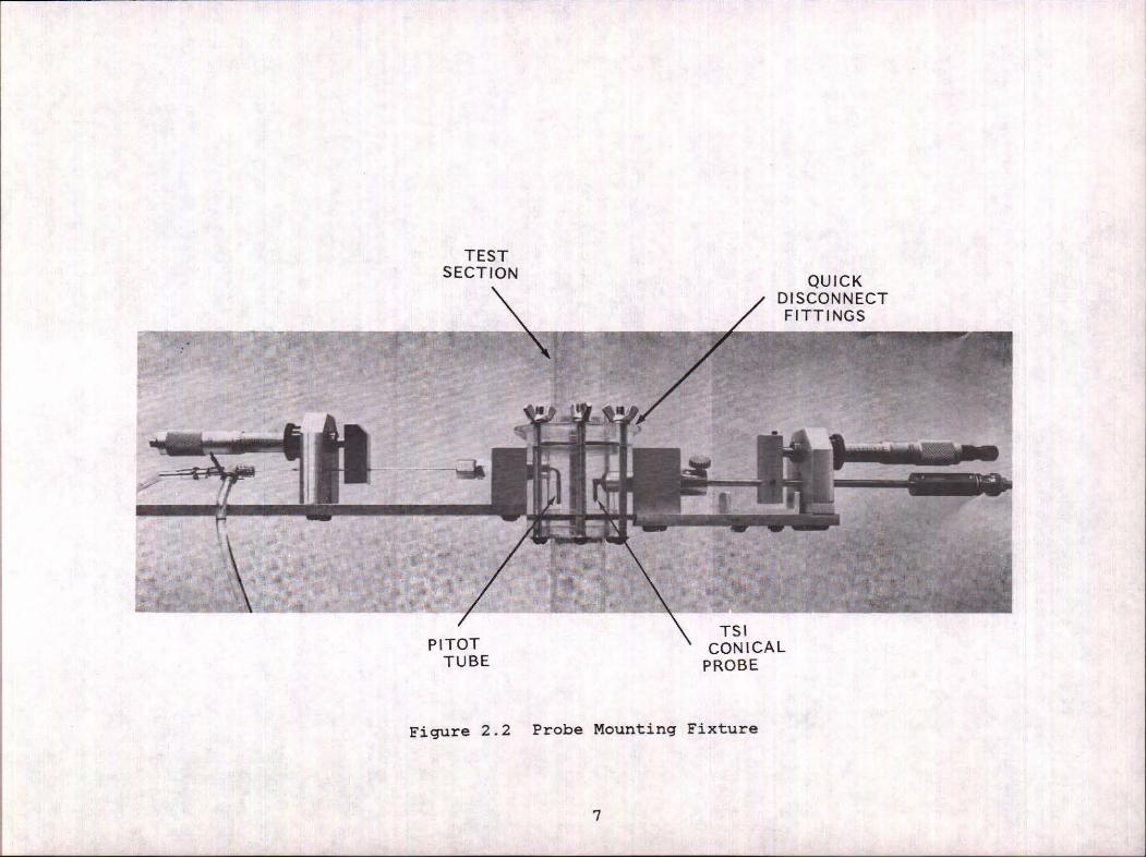
the entire diameter via an identical path. As shown in Fig.

2.2 , a special fixture was constructed to hold the

traversing mechanisms. This fixture can be easily removed

from the loop to facilitate the periodic removal of

contamination from the hot-film sensor. Linear micrometers

with shift slots enable the conical probe and the pitot tube

to traverse the entire diameter with accuracy of one mil (1

x 10- 3 inch). Two grooves are made on the inner walls of the

fixture so that both the conical probe or the pitot tube can

be recessed into the groove while the other is being

traversed.

Near the bottom of the loop, an iron-constantan

thefmocouple is inserted to monitor the inlet water

temperature. Keeping constant water temperature is essential

because the calibration curve for the hot-film anemometer is

sensitive to the fluid temperature.

HOT FILM ANEMOMETRY

Fig. 2.3 shows the dimensions of the conical probe and

the sensing element. The sensing element is a quarzt coated

platinum film on the conical substrate near the tip. The

film is electrically connected to a TSI 1050 anemometer. The

anemometer draws power from and displays the bridge output

on a TSI 1051 Readout and power supply module. In the

6

TEST SECTION

PITOT TUBE

Figure 2.2

QUICK DISCONNECT FITTINGS

TSI CONICAL

PROBE

Probe Mounting Fixture

7

- • 1 \• ..

PLATINUM FILM THICKNESS

QUARTZ FILM THICKNESS

----------

ALL DIMENSIONS IN INCHES

0.2 MICRONS

4 MICRONS

~-- 0.060----

QUARTZ SUBSTRATE

1231 CONICAL SENSOR

Figure 2.3 Dimensions of The Conical Probe

8

anemometer, there are three wheatstone bridges to select

from, depending on the power dissipation rate at the sensor.

It was found that bridge #1, the least powerful but the most

sensitive bridge, was the most suitable for two-phase

turbulence measurement.

SIGNAL CONDITIONING

The anemometer bridge output is also internally

connected to a TSI 1051 Signal conditioner. The signal

conditioner has both low-pass and high-pass filters and

zero-suppression capability. The bridge output range, 0 to

15 volt, is too large for the input range of the FM

recorder, -1.41 to 1.41 volt. For single-phase turbulence

data, the signal can be biased so that the turbulence

portion of the signal is within the input range of the

recorder. However, for two-phase measurements, the voltage

variation due to phase change is greater than 2.42 volt, the

input range of the recorder. For this case, the signal was

attenuated using a custom-built voltage divider before being

fed into the FM recorder.

Because the FM recorder has a fixed noise-tc-signal

ratio, 0.3%, the accuracy of the signal is best preserved

when the 2.42 volt input range is fully utilized to record

the turbulence portion of the signal. For single-phase

9

signals, the noise levels can be easily reduced to minimal

levels relative to the liquid turbulence level by simply

suppresing the DC component of the signal. This is not the

case for two-phase flow, where the signal fluctuation due to

phase change is about 10 times larger than that of liquid

turbulence. A sizable noise level on the liquid turbulence

signal was observed when the two-phase signal was

attenuated, stored in the FM recorder, and then played back.

One solution was to reduce the signal fluctuation due to

phase change by clipping the signal at the bottom. Indeed,

except for phase determination, the gas phase signal is of

no interest. Fig. 2.4 is the circuit diagram of such a

clipping circuit and Fig. 2.5 illustrates how this clipping

circuit improves the signal-tc-noise ratio for two-phase

flows.

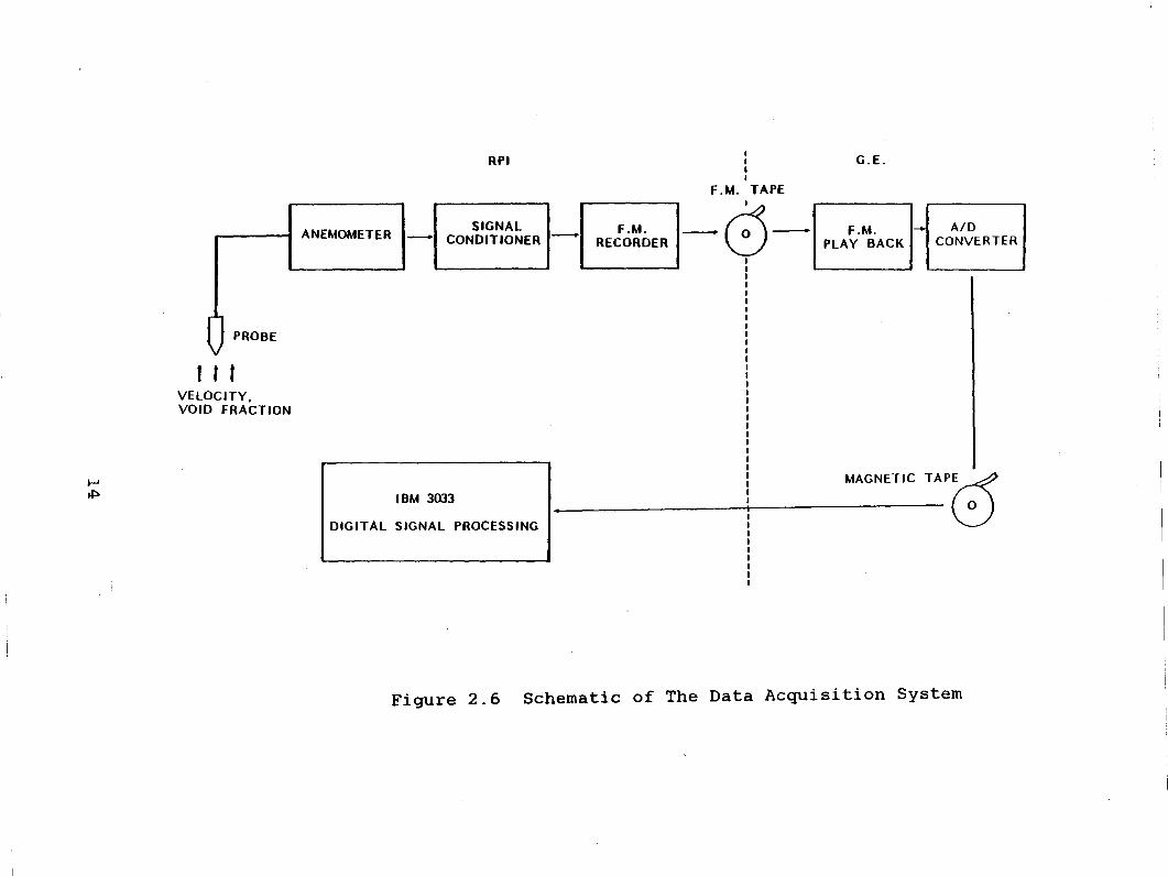
DATA ACQUISITION SYSTEM

The conditioned signal was recorded on a Honeywell 5200C

14-channel FM recorder. Subsequent to the experiment, the

analog tape was played back into a A/D converter, which

wrote the digital data on a magnetic tape. The A/D converter

used is a part of a Hewllet-Packard Fourier Analyzer system

at the General Electric Co. It can digitize and write up to

4 signals simultaneously at a rate in excess of 10 kHz. The

10

~ ~

ANEMOMETER SIGNAL

-15V

CLI PPED SIGNAL

lK ~ , 1N914B 1

+15V

lK l CLIPPING VOLTAGE -0.7V

--

Figure 2.4 Circuit Diagrarn of The Clipping Circuit

ORIGINAL SIGNAL FROM THE ANAMOMETER

v

TIME

SUPPRESSION OF THE ZERO

v

TIME

CLIPPING THE SIGNAL AT THE BOTTOM

v

TIME

Figure 2.5 Siqnal Conditioninq of Two-phase Data

12

digital tape was then processed on a IBM 3033 computer.

Appendix-C describes how the Hewlet-Packard generated tape

was read with IBM computer. Fig. 2.6 shows schematic diagram

of the data acquisition system ..

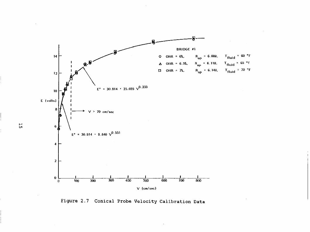
PRELIMINARY CALIBRATION OF THE ANEMOMETER

It is a standard practice to relate the anemometer out­

put voltage to the fluid velocity by King's Law,

where,

E = anemometer output voltage,

V = fluid velocity,

A,B,n = calibration constants.

( 2. 1)

As shown in Fig. 2.7 our preliminary calibration data indi­

cates that a different power law applies in two different

regions of Renolds nurnber; n = 0.551 for Re < 10,000, and n

= 0.333 for Re > 10,000. The parameters A and B were found

to be sensitive to the fluid temperature and the probe's

overheat ratio. For our preliminary calibration curve, the

parameters A and B were determined such that the two

different power laws match at Re = 10,000. In practice the

actual point-to-point calibration data will be used.

FREQUENCY RESPONSE OF THE ANEMOMETER

13

..... ,p.

PROBE

t r r VElOCITY, VOID FRACTION

RPI

SIGNAL ANEMOMETER 1--1 CONDITIONER

IBM 3033

DIGITAl SIGNAl PROCESSING

F.M. RECORDER

1 1 1 1

F.M. TAPE

-~-

1 1 1 1 1 1 1

1 1 : 1 1 1 1 1 1

G.E.

F.M. , ...... , AID PlAY BACK CONVERTER

MAGNETIC TAP~

Figure 2.6 Schematic of The Data Acquisition System

~ ll1

14

10

E (volts)

6

4

2

0

----------­~3 g .. W :a/\

ir' 0.333 11 914 • 25.035 v E' = 30.

' V > 70 cm/sec

E' = 30.914 • 9.840 v0.551

~­~

BRIDGE #1

0 OHR = 6\, R0

P = 6.08!2,

b. OHR = 6.5%, R0

P = 6.1H2,

[] OHR = 7't., R0

P = 6.1412,

lOO 200 Q nnn

V (cm/sec)

Figure 2.7 Conical Probe Velocity Calibration Data

T fluid = 60 oF

T fluid = 65 oF

T fluid = 70 oF

Because generating flow fluctuations of known amplitude over

a wide range of frequencies is difficult, the electrical

testing technique suggested by Freymuth [3] is usually used

to estimate the frequency response of the anemometer. With

the probe immersed in a single-phase(liquid) flow of typical

velocity, the amemometer bridge is excited by a sine wave

signal. The frequency response of the sine wave signal is

then used to estimate the frequency response of the system

to velocity fluctuations. In particular, theory [3] says

k that the electrical testing result should follow a f 2 curve

for a flat frequency response to velocity fluctuations. It

can be seen from our electrical testing data, Fig. 2.8 ,

that the frequency response stays flat up to about 29 kHz.

However, this frequency response is for a single-phase

signal. For two-phase signal, where interface penetration

causes a sudden and large change of the signal, the

electrical testing technique may not apply. Indeed, the

overshoot and signal decay observed in our two-phase data

indicate that the frequency response may be much lower for

large amplitude fluctuations such as those encountered

during phase change.

NOISE and ACCURACY

Noise, linearity, and drift problems are inevitably

16

BRIDGE

LOG(E/Et ) Rop

Tfluid

Et

10 v max

Re

#1

= 6.08!2

= 71 OF

= 4 volts

= 57.4 cm/sec

= 7200

FREQUENCY (Hz)

/ /

' -3db

f0P = 29 kHz

Figure 2.8 Electrical Testing Result of The Conical Probe

17

introduced when the analog signal is recorded, played-back,

and digitized. To determine the magnitude of these errors,

three constant voltages, 0.400 V, 0.300 V, and 0.400 V were

recorded for 10 second intervals. The recorded signals were

then digitized at 10 kHz. 10 records(one record contains

1024 digital data points) of each run were examined to

compute the mean and the standard deviation. The result is

as follows:

Signal 0.400 v 0. 300 v 0.400 v

Mean(V) 0.3571 0.2665 0. 3554

S.D. (V) 0.0024 0.0025 0.0024

Since the input range of the recorder is ±1.41 V, 0.0025 V

noise level corresponds to signal/noise ratio of 55 dB,

which is better than the specified signal/noise ratio of the

recorder, 50 dB. The two 0.400 V results indicate

reproducibility. The signal drifted about 2 mV in 10 second.

A 0.10 volt difference in the analog signal corresponded to

only 0.09 volt difference in the digitized form. To monitor

and correct for these noise and drift, constants voltage

signals will be inserted in between each experimental run.

SIMULTANEOUS DIGITIZATION

To test simultaneous recording and digitization of two

signals, a 1 kHz square-wave signal was recorded into two

18

------------- --- ---

channels, channel 1 and 3, of the recorder and was sampled

at 200 kHz. The plot of the digitized signals in Fig. 2.9

shows a shift of less than 0.01 ms. It should be noted that

with the H.P. system to ensure simultaneous digitization

either even number channels or odd number channels must be

used together. That is, ether channel 1, 3, and 5 or channel

2, 4, and 6 must be used for three channel simultaneous

recording.

19

----------------------------

N 0

0 ._ --- -- ·-

1 2

Time(ms)

3

Figure 2.9 Simultaneous Digitization Result of A Square Wave

CHAPTER 3

PHASE DETERMINATION TECHNIQUE

After the anemometer output signal is conditioned,

digitized, and written on a magnetic tape, the remaining

data reduction is done by a set of FORTRAN programs. The

programs perform basically two tasks: recognize and

separate-out segments of the signal corresponding to liquid

phase, and compute parameters of interest from the liquid

phase data. This chapter is concerned with the former of the

two. First, we will discuss how void passages shows up in

the a.nemometer output signal. Then, a digital technique to

automate this signal interpretation will be described.

Finally, the computer progams and sorne preliminary results

will be presented.

ANEMOMETER SIGNAL INTERPRETATION

The basic problem in interpretating two-phase data has

to do with dynamic response of the probe and with the

interaction of surface tension with the probe. Because the

beat transfer coefficient between the probe substrate and

the arnbient fluid is lower in gas than in liquid, the

temperature distribution in the substrate, bence the beat

conduction from the sensor to the substrate, undergoes a

21

substantial change during void passage. This may result in

an unrealistic reading of the liquid phase velocity imrnedi­

ately following probe entrance into liquid phase from gas

phase. Only after the probe substrate achieves a new

equilibrium temperature distribution in the liquid phase,

will the signal start to read a realistic liquid phase

velocity.

When gas bubbles approach and intersect the probe,

surface tension causes them to deform around the probe tip,

and thus immediate penetration of the interface does not

occur. Actual penetration, and consequently a sudden dip in

the signal, occurs much later in time, when the imaginary

undeformed interface is well advanced along the probe. This

phenomena has been throughly investigated by Delhaye [4] who

took high-speed pictures(2000 frames per second) of the

bubble passages and the probe output signal displayed on an

oscilloscope. His findings are summarized bellow.

On Fig. 3.1 Delhaye has observed the bubble passage

through a vertical conical probe. Before tA , the probe

responds to the liquid velocity and turbulence. At tA , the

probe begins to sense the bubble due to buyancy-induced

liquid displacement, and the signal increases gradually. At

tB the imaginary bubble interface reaches the sensor element

on the probe. However, the actual interface deforms around

the probe tip and penetration does not occure until tc at

22

1 1 ---- LJQUID---+1+----+--- GAS ---4--l--li----LIQUID

Figure 3.1 Schematic of Bubble Passage Through A Conical Probe [4]

23

which point the signal drops. At t 0 , the rear surface of

the bubble touches the probe tip. A rapidly rising miniscus

cools the sensor from t 0 to tE . At tF , the imaginary rear

interface reaches the sensor, and at tG the probe is fully

irnrnersed in liquid. Delhaye measured the average durations

tC-tB and tF-tE :

tC-tB = 1.3 ms

tF-tE = 2.0 ms

Our bubble passage data has similar features as

Delhaye's except for the much higher posterior overshoot.

Rapid meniscus cooling ,as suggested by Delhaye, does not

seem to be soley responsible for the overshoot because the

overshoot, if converted to velocity, can reach upto 250

cm/sec for mean liquid phase velocity of 50 cm/sec. Rather,

the dynamic response of the probe substrate to the medium

change may contribute to the transient behavior. Thus, the

time at which the probe signal returns to read the actual

liquid phase velocity cannet be determined by visual exami­

nation of the bubble passage. Instead, transient heat

transfer analysis of the substrate and the sensor may be

needed to learn more of this phenomenon.

Another disagreement lies in the time the rear surface

takes to travel from the probe tip to the sensor, tF-tD .

According to Delhaye, the overshoot decays away completely

in this time interval and the liquid phase data can be taken

24

from tF on. For the experimental conditions for which our

data was obtained, a bubble travelling at 50 cm/s can cover

the distance from the probe tip to the sensor, 0.026 cm, in

0.5 ms. However, visual examination of many bubble passage

signals indicates that the overshoots decays away only after

2.0 ms. Therefore, we conclude that the overshoot persists

even after the rear surface of the bubble passes the sensor.

Delhaye's interpretation was slightly modified before

being applied to our data. Fig. 3.2 is a schematic of a

typical signal and the corresponding position of the bubble

with respect to the probe's sensor according to the modified

interpretation. The time tB represents the time at which the

imaginary bubble interface crosses the sensor. The interface

is penetrated at tc . At ~ , the probe tip contacts the

rear surface of the bubble. At tE , which does not

necessarily coincide with the peak of the overshoot, the

imaginary rear interface reaches the sensor. At tG the

signal returns to read the liquid phase velocity.

Unfortunately, sharp changes in the signal occur only

at tc and tD i the other times, tB , tF , and tG must be

estimated using ether means. Delhaye suggested 1.3 ms for

tC-tB . However, this time interval can be expected to be

related to the velocity of the liquid phase and the bubble

size. The time interval tF-tD can be approximated by

dividing the distance from the probe tip to the sensor by

25

....

- LIQUIO ----1·------- GAS ----~------- LIQUIO-

Figure 3.2 Modified Schematic of Bubble Passage Through A Conical Probe

26

the mean axial liquid phase velocity. Time tG , the time at

which the signal returns to reflect the realistic liquid

phase velocity, may be determined from the analysis of

dynamic response of the probe. At present such analysis is

not available. Therefore, the average duration of the

overshoot was emprically determined. About 2 ms after t 0 the

overshoot seemed to decay away to the level of the liquid

phase, thus tG ~ t 0 + 2 ms.

DIGITAL IMPLEMENTATION OF THE PHASE DETERMINATION TECHNIQUE

To determine the phase of the probe signal, one must be

able to detect tc and t 0 . Past investigators have used

either level thresholding or slope thresholding. In level

thresholding, the gas phase is triggered whenever the signal

dips below a specified level and is terminated when the

signal rises above that level. Phase determined using this

method is not precise but the method is stable in the sense

that while it may fail locally, it always succeeds globally.

In slope thresholding, the fact that tc and t 0 accompanies

much steeper signal changes compared to that of liquid phase

turbulence is used to trigger the phase indicator on and

off. This method, when it works, detects tc and t 0 quite

precisely. However, it is unstable in the sense that a sin­

gle failure to trigger on interface passage leads to

27

complete failure of the method.

Both methods were tried to our data and it was found

that the best method was a combination of both. That is,

slope thresholding was used to trigger on and off the gas

phase and then in each phase, excluding transition periods,

each data point also was tested against level thresholding.

In this way, precise slope thresholding was used most of

time, and occasional failure of the method was immediately

corrected by level testing. This dual method is herein

termed the "modified slope" thresholding method.

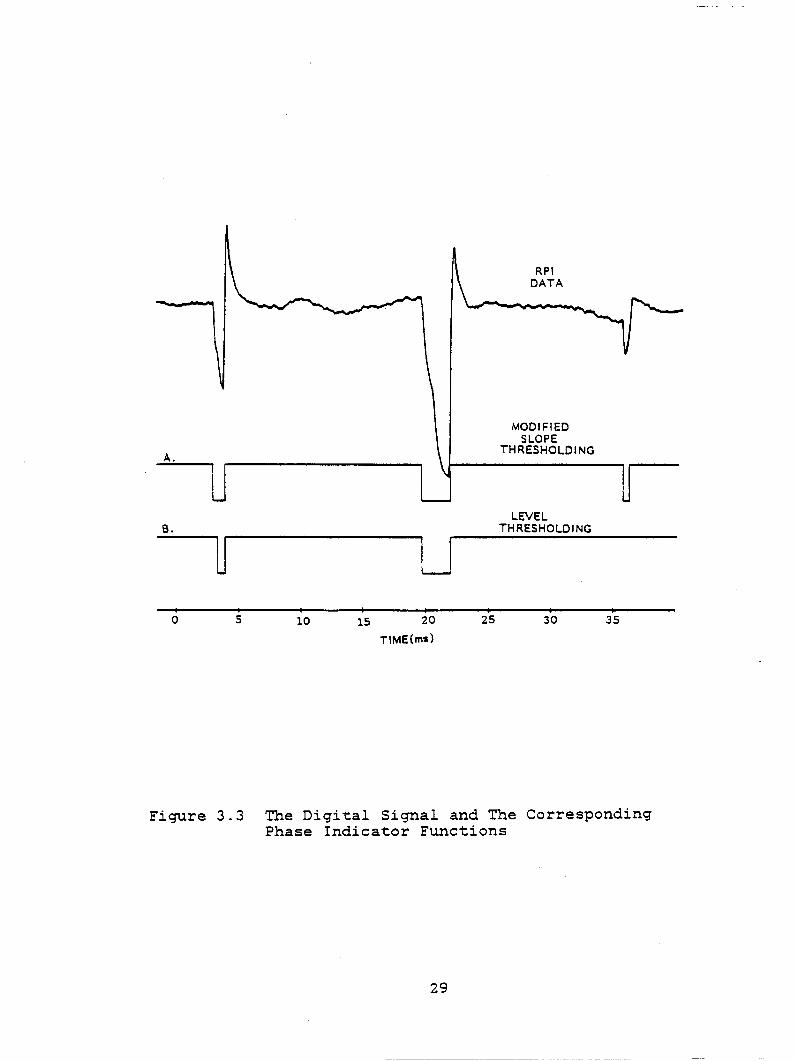
Fig. 3.3 shows an actual probe .signal with the two cor­

responding phase indicator functions generated using two

different methods: curve-A by level thresholding and curve-B

by rnodified slope thresholding (note that tC-tB and tF-tD

were arbitrarily set to zero for simplicity). It can be seen

that level thresholding method triggers at delayed time, as

seen by the first bubble passage, and it misses small

bubbles, as seen by the third bubble passage.

DESCRIPTION OF COMPUTER CODES, VOIDl and VOID3

The rnodified slope thresholding method is used for

phase determination in two computer codes, VOIDl for

single-sensor probe data and VOID3 for three-sensor probe

data. Once the phase is correctly determined, the

28

A.

B.

~ 0 5

Figure 3.3

- --- - ---------

u 10 15 20 25

TIME(ms)

RPI DATA

MODIFIED SLOPE

THRESHOLOING

LEVEL THRESHOLDING

30 35

The Digital Signal and The Corresponding Phase Indicator E'unctions

29

computation of the various flow parameters is

straightforward. VOIDl computes the local void fraction, a ,

the axial mean liquid velocity, U, and the

root-mean-square(RMS) value of the velocity fluctuation

about the mean, u 2 . It also generates the peudo liquid

phase indicator function, x1n). VOID3 computes a and the

variance matrix of the liquid velocity fluctuation about the

mean, VAR(v). The phase indicator function is also generat­

ed. To monitor the algorithrn, these programs also output

running statistics such as the maximum void size, the maxi­

mum gas phase signal, the minimum liquid phase signal, and

the steepest slope in liquid phase.

RESULTS

VOIDl has been thoroughly tested against two-phase data

obtained on the test facility previously described. At

present .there are no other means to verify the flow parame­

ters computed by VOIDl. However, the running statistics of

the program indicates that the algorithrn seems to work cor­

rectly. Since only single-sensor probe data is currently

available, VOID3 was tested against hypothetical data and

was found to give the expected results.

At present, there are no systematic way of determining

the proper level and the slope threshold values available.

30

They have been determined using qualitative judgement after

visual examination of the probe output signal. A more

systematic approach may be found in the probability plot of

bath the amplitude the slope of the signal, although such a

method has not been developed to date.

31

CHAPTER 4

DIGITAL COMPUTATION OF FLOW PARAMETERS

The digital data is assumed to be a sequence of length

N, whose index ranges from 0 to N-1. The index is related to

the time through the sampling period. Throughout this

chapter index and time are used interchangably. Also the

equal sign" =" is used to mean "is computed by".

ONE DIMENSIONAL DATA

Liquid Phase Indicator Function, X(n):

= l 01

X(i) 1, otherwise

Local Void Fraction, a

N-1

a = 1 - ~ X(i)/N

i=O

Mean Liquid Phase Velocity, U:

Data points in the overshoot region, although they

belong to liquid phase, should be excluded in computing

32

(4.1)

(4.2)

liquid phase flow parameters because it is felt they do not

represent realistic liquid phase turbulence. Let us define a

pseudo liquid phase indicator function by,

~' 0, ( tB ~ i ~ tG)

x+(i) = 1, otherwise

Then, the axial mean liquid phase velocity is given by,

u = N-1 , ·~ N-1 t; x•(i)U(i)~ t; x•(iJ

(4.3)

(4.4)

where the intantaneous axial liquid phase velocity, U(i), is

computed from the data, E(i), based on the calibration.

The RMS Value of The Liquid Phase Veloci ty Fluctuation, ./ u 2 :

N-1

w =[ L i=O

., ;N-1 x•(i)(U(i)-Ü)jl t;

THREE DIMENSIONAL DATA

(4.5)

The measurement of three dimensional liquid velocity

fluctuation in two-phase flow using a three-sensor probe

33

gives three sequences of data, E1 (n), E2 (n), and E 3 (n). For

each sequence of data, the same phase determination

technique can be applied and obtain three liquid phase

indicator functions X1 ,X 2 , and X3 as well as three pseudo

liquid phase indicator functions xi(n), x;(n), and X~(n).

Local Void Fraction, a

N-1

a= 1- ~ Xt(i)/N

i=O

Reynold's Stresses:

For a given flow condition, the signal fluctuation

( 4. 6)

about the mean for sensor i, e. , is assumed to be related ~

to the velocity fluctuation by the following linear equa-

tiens,

where

el(n) = alu(n)/Ü + elv(n)/Ü + olw(n)/Ü

e2(n) = a2u(n)/Ü + e2v(n)/U + o2w(n)/Ü

ea(n) = aau(n)/Ü + eav(n)/Ü + oaw(n)/Ü

u(n), v(n), and w(n) are velocity fluctuations in

( 4. 7)

axial, radial, and azimuthal directions, respectively. The

directional sensitivities ai 1 ei 1 and oi must be deter­

mined from experiment [5] . It is convenient to cast

34

equation (4.7) into matrix formas,

§(n) = A v(n)

where,

and,

Then,

e(n) = (edn),e 2 (n),e 3 (n)) T

v(n) = (u(n),v(n),w(n)) T

1 [a1 ~1 r1]

A = U cx2 ~2 r 2

cx3 ~3 r3

y(n) = A- 1 ~(n)

(4.8)

(4.9)

The variance matrix of v can be expressed in terms of the

variance matrix of E as follows.

[

U2 uv uw]

VAR(v) = uv ~ vw

wuwv~

T = ~(y Y. )

Substituting equation (4.9),

= .;,(A-1 ~eT A-1T)

= A-1 .!(.§. .§.T) A-1T

= A- 1 VAR(~) A_ 1T -

However, by definition,

VAR(~) = VAR(E_)

=,;<~ET) - E.CE;) (~(~) )T

35

(4.10)

(4.11)

where ~(E) is the expectation vector of E,

(4.12)

Thus, from equations (4.11) and (4,10),

( 4. 13)

Equations (4.12) and (4.13) are used in VOID3 to compute the

Reynold's stresses which are obtained by multiplying VAR(y)

by minus the density of the liquid phase.

Anisotropy Factors:

Recall that the ultimate goal of the on-going project

is to experimentally verify the relationship Lahey and Drew

have previously derived (2] between the void distribution

and the liquid phase turbulence structure in two-phase flow.

Although the relationship applies to flows in channels of

arbitrary cross section, at present we are interested in the

flow through a circular pipe. In cylinderical coordinates,

the relationship is given by (2],

36

r

1-q (1-a)K qq rr dr} f

F (r' )-F (r')

t r'F (r') rr

R

(4.14)

where

C 1 = constant of proportionality between liquid and

vapor phase Reynolds stresses,

K1 = liquid phase turbulent kinetic energy

= !s p 1

( U"Z +vz + w2 ) ,

E' rr = Vl 1 ( U2 + VZ: + ~ ) '

E' qq = W2 1 ( ~ + v' + w' ) ,

and C2 is the constant of integration.

The integration inside the exponent accounts for the

anisotropy of the turbulence. To determine the degree of

anisotropy, one has to measure the Reynold's stresses along

the entire radius of the conduit.

37

CHAPTER 5

SPECTRAL ANALYSIS OF DIGITAL DATA

Spectral analysis of signals from both single-sensor

and three-sensor probes provides valuable information about

the turbulence structure of the flow, about the frequency

content of the signal, and the bubble convection from one

sensor to another in the case of a three-sensor probe. The

frequency composition of the signal, in turn, determines the

minimum digitization rate required to avoid aliasing. Any

noise with characteristic frequency shows up as a

distinctive peak in the power spectrum. Thus, spectral

analysis is useful in designing the experiment.

Spectral functions are defined for continuous time

signals. Our data, however, is a digital(discrete tirne)

signal derived by periodically sarnpling the probe output

voltage. Hence, we can only estirnate the exact spectral

functions from the digital data. Accuracy of the estimates

depends mainly on the length of the data record and the

digitization rate. Ideally, both the data record length and

the digitization rate should be very large. Unfortunately,

practical considerations often determine the record length.

This chapter discusses the effects of the finite record

length of data and the digitization rate on spectral func­

tions estimation.

38

The fluctuating liquid velocity at the sensor is as-

sumed to be erogodic. That is, the time average is equiva-

lent to the corresponding ensemble average. For sufficient

long record lengths, this assumption is valid as long as the

flow conditon stays constant. Throughout this chapter, it is

assumed that the flow on which the spectral anaysis is

performed is erogodic.

AUTO AND CROSS-CORRELATION FUNCTION, Rxy(t)

The cross-correlation function of two continuous time

signals, x(t) and y(t), is given by,

= lim T-+-

T

i ~ x(t)y(t+t) dt

0

( 5. 1)

When x(t) and y(t) are identical, we get an autocorrelation

function, Rx{t). Usually, the means are removed from the

signals before performing spectral anaysis. The correspond-

ing correlation functions for the fluctuating part of the

signals are called autocovariance and cross-covariance func-

tiens. Sorne of the important properties of the

autocovariance function are [6] :

R { -T) = R { T) x x ( 5. 2)

39

a 2 =R(O) (5.3) x x lim R (~) = 0 (5.4) ~..... x

For the cross-covariance function, the following property is

useful for computational purpose,

R (-t) = R (t) xy yx ( 5. 5)

AUTOCORRELATION FUNCTION AND LIQUID TURBULENCE SCALES

If a flow has a uniform mean velocity U, such that U >>

uz, the autocorrelation R (~) for the velocity fluctuation u

u(t) at a fixed point can be used to determine the so-called

integral scale of the liquid turbulence, Af' and the

dissipation scale, Àf (Appendix-A). That is,

and,

1

17 =

..

1 2R (O)U 2

u

POWER SPECTRAL DENSITY FUNCTION, Gx(f)

(5.6)

( 5. 7)

The Fourier transform of an autocorrelation function

yields the power spectral density function. That is,

40

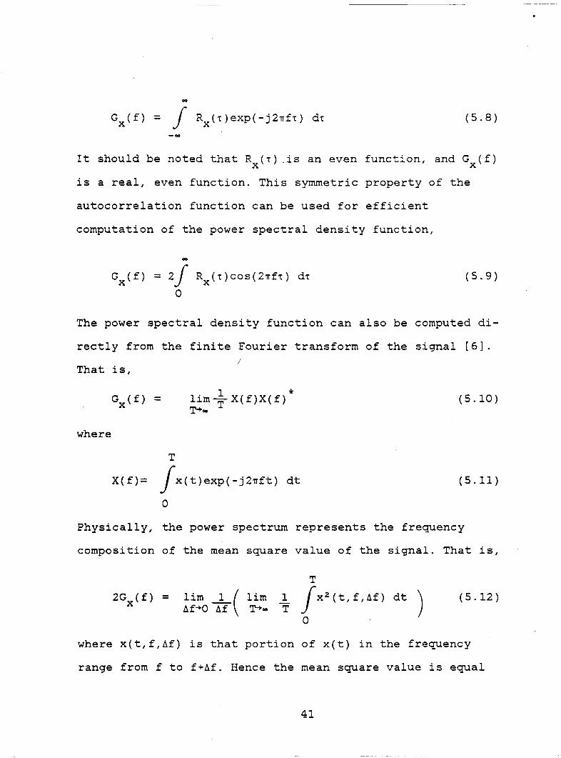
00

-oo

R (t)exp(-j2~ft) dt x ( 5. 8)

It should be noted that Rx(t) _is an even function, and Gx(f)

is a real, even function. This symmetric property of the

autocorrelation function can be used for efficient

computation of the power spectral density function,

00

R (t)cos(2~ft) dt x ( 5. 9)

The power spectral density function can also be computed di-

rectly from the finite Fourier transform of the signal [6]. /

That is,

where

T

lim i X(f)X(f)* ~-

X(f)= ~x(t)exp(-j2~ft) dt

0

(5.10)

(5.11)

Physically, the power spectrum represents the frequency

composition of the mean square value of the signal. That is,

lim 1 ( lim 1 6f-+O 6f ~00 T

T

~x2 (t,f,U) dt )

0

(5.12)

where x(t,f,6f) is that portion of x(t) in the frequency

range from f to f+6f. Hence the mean square value is equal

41

to the total area under a plot of the power spectral density

function versus frequency. Usually the power spectral

density function is computed for only the fluctuating part

of the signal because the mean value shows up as a spike at

the orgin of the power spectra. That is,

CROSS-SPECTRAL DENSITY FUNCTION, G (f) x y

(5.13)

Just as the power spectral density function of a single

signal is the Fourier transform of the autocorrelation func-

tion, so the cross-spectral density function of a pair of

signals is the Fourier transform of the cross-correlation

function.

00

(5.14) -oo

Unlike the power spectral density function, which is real,

the cross-spectral density function is generally complex.

The typical cross-spectral density plot(ie. cross-spectrum)

consists of two parts, magnitude and phase.

42

COHERENCE FUNCTION, ~ (f) x y

To give physical significance to the cross-spectral density

function a real quantity, the coherence function is defined

as,

0 ( f) 2

x y = IG (f) 12

x y Gx(f}Gy(f)

(5.15)

The coherence function, which takes value from zero to one,

gives a measure of the correlation between x(t) and y(t) at

different frequencies. x(t) and y(t) are fully coherent at a

frequency if the coherence function at that frequency is

unity.

COMPUTATION OF CORRELATION ESTIMATES

Correlation functions as previously defined cannot be

applied directly to our data because, first, the data is a

discrete time signal derived from periodic sampling of the

analog (anemometer) output and, second, the data has finite

length. This section presents the digital estimation methods

and examines the finite length and discrete time effects

on the accuracy of the spectral estimation when the methods

is applied to our data.

For a digital signal of length N the M-point

cross-correlation estimate is given by

43

N-m-1 " 1 L /'. A R (rn) =-N x(n)y(n+m) xy -rn

n=O

, 0 s rn s M-1 (5.16)

where Ms N. Equation (5.5 ) is used to compute the

cross-correlation estimate for rn < O. The digital signals

x(n) and y(n) are related to the corresponding analog signal

by

x(n) = x(nT)

y(n) = y(nT)

where T is the sampling period. Clearly, if N is ,.

(5.17)

sufficiently large, Rxy(m) is just a uniform sampling of Rxy

( t ) • Th at i s ,

(5.18)

A

Since Rxy(m) estimates Rxy{t) exactly at M points, as long

as the sampling period is short enough to follow any erratic

behavior of the true autocorrelation, and the true

autocorrelation vanishes at t > MT, the estimation is a

good one.

Appendix-B describes how Fast Fourier Transform(FFT)

techniques can be used to efficiently compute the equation

(5.16). Computing equation (5.16) directly takes time

proportional to NM. But using FFT the computing time is

proportional to (N+M)Log 2 (N+M). For N=5120 and M=256, which

is our typical figure, the computation saving is 95%.

44

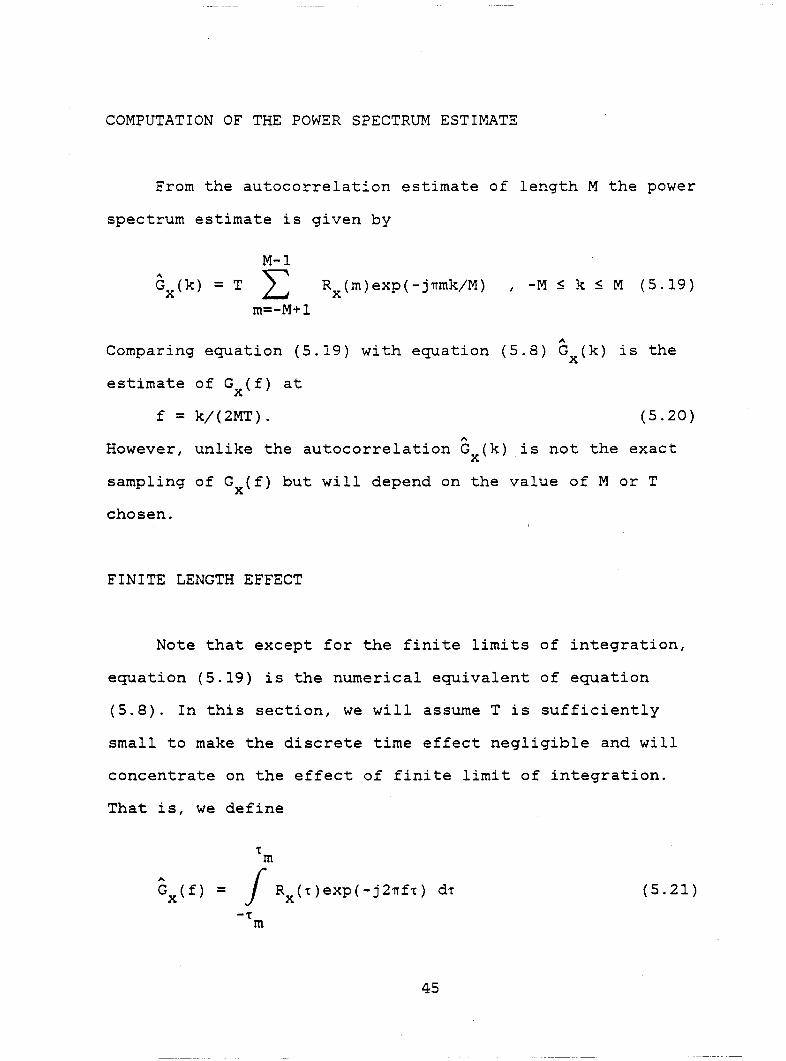
COMPUTATION OF THE POWER SPECTRUM ESTIMATE

From the autocorrelation estirnate of length M the power

spectrurn estirnate is given by

M-1

Gx(k) = T L rn=-M+l

R (rn) exp ( - j 1rrnk/M) , - M ~ k ~ M ( 5 . 19 ) x

"" Cornparing equation (5.19) with equation (5.8) Gx(k) is the

estirnate of Gx(f) at

f = k/(2MT). (5.20)

" However, unlike the autocorrelation G (k) is not the exact x

sarnpling of Gx(f) but will depend on the value of M or T

chosen.

FINITE LENGTH EFFECT

Note that except for the finite lirnits of integration,

equation (5.19) is the nurnerical equivalent of equation

(5.8). In this section, we will assume T is sufficiently

srnall to rnake the discrete tirne effect negligible and will

concentrate on the effect of finite lirnit of integration.

That is, we define

"C rn

Gx(f) = ~ Rx(t)exp(-j21Tft) dt -"(

rn

45

(5.21)

,... To see how the estimate G (f) is related to the true power x

spectral density function G (f) , we can rewrite the previ­x

ous equation as,

00

-oo

W(1)R (•)exp(-j2Tif1) d1 x

where W(1) is a window function defined by,

W( 1) = { 1,

0, otherwise

A

(5.22)

(5.23)

It is clear from (5.22) that Gx(f) is the Fourier transform

of the product of the window function and the

autocorrelation fuction. From the properties of Fourier

transform, multiplication in time domain is equivalent to

convolution in frequency domain. Therefore, A

Gx(f) = Gx(f)*w(f)

00

=f (5.24)

-oo

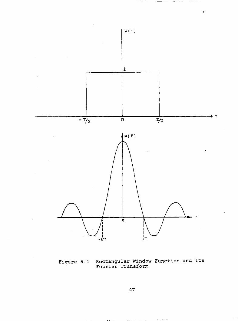
where w(f) is the Fourier transform of W(1). Fig. 5.1 shows

the rectangular window function and its Fourier transform.

The effect of convoluting the true power spectrum with the

Fourier transform of the window function is to cause

"leakage" by spreading the true power spectrum with the

weighing window function. The Fourier transform of the

46

w( r)

.l

0

f.IJ(f)

Figure 5.1 Rectangular Window Function and Its Fourier Transform

47

rectangular window function shows large undesirable side

lobes. To suppress this leakage problem, the window function

must be modified in the time domain. Technique for designing

a better window function involves mainly reducing the side

lobes at the expense of broader main lobe. Table 5.1 lists

three other windows which were implemented as an option in

the computer program POWER.

DISCRETE TIME EFFECT

Let us consider a Fourier transform pair of a

continuous time signal, x(t) and X(f).

-X(f) =f x(t)exp(-j21Tft) dt (5.25)

-...

~

x(t) =f X(f)exp(j21Tft) df (5.26)

-~ A

derived by sampling Suppose a discrete ti me signal x(n) is

x(t) with period T,

" x(n) = x(nT). (5.27)

A Fourier transform pair can also be defined for the

descrete time signal and its frequency-domain representa-

ti on.

48

1(:> \{)

WINDOW TYPE

RECTANGULAR WIN DOW

BARTLETT WIN DOW

HANNING WIN DOW

HAMMING WINDOW

N-POINT WEIGHTING FUNCTION SHAPE OF THE WINDOWS

W(i) = 1

W(i) = 1 _ 2 1 i - (N+1)/2 1 N•l

2j-N-1 W(i) = 0.5 + 0.5 COS( u N-1 )

W(i) = 0.54 + 0.46 COS( 11 ~~~-1 )

~-

Table 1 List of Window Functions

.. " X(f') =

... x(n)exp(-j2~f'n) (5.28)

n=--

~ " x(n) =f .....

X(f' )exp(j2~f'n) df' (5.29)

-~

Then, the sampling theory gives the relationship between

" X(f') and X(f) as [7]

.. X( f') = 1/T 2: X( f+r/T) (5.30)

r=-..

where,

f = f'/T. (5.31)

The relationship between the continuous-time Fourier trans-

form and the Fourier transform of a sequence derived by

periodic sampling is depicted in Fig. 5.2 . The Fourier

transform of the discrete-time signal is the scaled down

version of the overlapping periodic repetitions of the A

continuous-time Fourier transform. Hence, for X(f') to

accurately ref1ect X(f), X(f) must be band limited; that is,

X(f) is zero outside a finte frequency band. Furthermore, to

recover whole range of X(f) spectrum the sampling rate must

be sufficiently high to avoid overlapping. That is,

(5.32)

where f 0 is the upper bound of the frequency band. The

50

--- -~------------------------------

FOURIER TRANSFORM OF A CONTINUOUS SIGNAL

X(f)

0 f. f

FOURIER TRANSFORM OF THE DISCRETE SIGNAL WHEN f. T > 1/2

x(n

1/T

.. ... 0 1/2 '\ f'

f. T

FOURIER TRANSFORM OF THE DISCRETE SIGNAL WHEN f. T < 1/2

x(n

1/T

1/2

Figure 5.2 Effect of Discrete Time Sampling On The Fourier Tranform of a Signal

51

minimum sampling rate, 1/T, which satisfy the inequality in

equation (5.32) is generally referred to as the "Nyquist

rate".

DETERMINATION OF DIGITIZATION RATE

In practice, truly band limited signals are rare and

the anemorneter output signal is no exception. However, X(f)

may fall rapidly past a certain frequency. In that case, a

sufficiently large sampling rate can make the folding back

from high frequency into the low frequency range of

interest, aliasing, neglegible. Initially, we digitized our

data at 10,000 samples per second. This was choosen to

resolve the rapid fall and rise of the signal during the

penetration of the phase interface. The power spectrum of

both single and two-phase signals (figure (5.11) and fig­

ure(S.12)) indicates that this rate is also more than

sufficient to avoid aliasing problem; for the single-phase

signal, the spectrum falls off rapidly to 10- 4 of the maxi­

mum value at the frequency of 500 Hz and then levels off;

for the two-phase siganl, the spectrum falls off to 10- 3 of

the maximum value at 1000 Hz.

52

SPECTRAL ANALYSIS OF SEGMENTED SIGNAL

In two-phase flow, the liquid phase signal is frequently

interrupted by void passages. Here, we are dealing with a

segmented signal where the data is not available between

each segment. Any attempt to interpolate the data in these

gaps will inevitably produce artificial components in the

power spectrum. We have adapted Lance's method [8] where

zeros are inserted into the missing parts. This method has

merit in that we know the effect of a zero insertion on the

"true" power spectrm.

Inserting zeros into the missing parts of data is

equivalent to applying rectangular-tooth window to the

"true" data. Note that the window function is identical to

the modified liquid phase indicator function, x+(n).

Specialize the equation (5.10) for power spectrum of

two-phase liquid velocity,

where

= liin 1/T T-+-

T * (~ u(t)X+(t)exp(-j2~ft)dt)

0

T

x (~ u(t)X+(t)exp(-j2~ft)dt) 0

* = 1/T [ T ( f) *x ( f) ] [ T ( f) *x ( f) ]

53

(5.33)

T(f) is the finite Fourier transforrn of u(t},

x(f) is the finite Fourier transforrn of x+(t).

Thus, the effect of a zero insertion is to srnooth the "true"

power spectrurn by convoluting the finite Fourier transform

of the "true" signal with the finite Fourier transform of

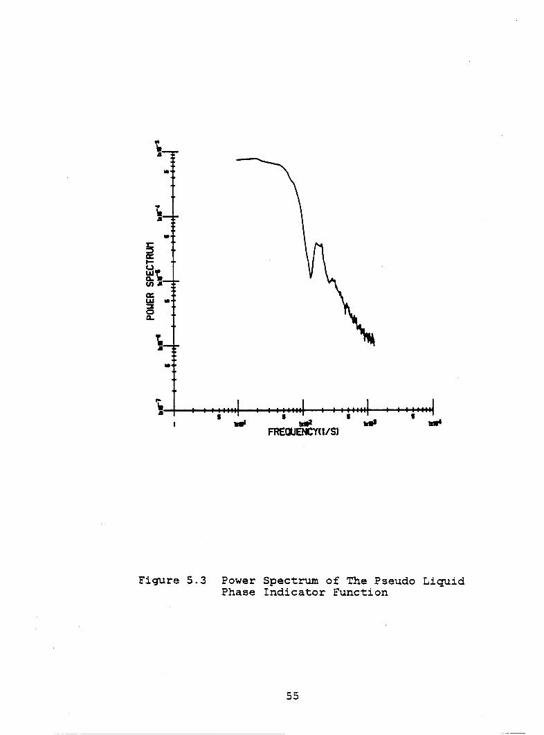
the pseudo liquid phase indicator function. Fig. 5.3 is the

power spectrurn of the pseudo liquid phase indicator function

of a sample two-phase flow data.

Fig. 5.4 is the schematic of the zero insertion process

employed to compute the power spectrum estimate of the

liquid phase fluctuating veloc'ity in two-phase flow. First,

the computer program VOIDl is run on the data to obtain the

mean liquid phase velocity and the pseudo liquid phase

indicator function. Second, the mean liquid phase velocity

is subtracted from the data. Third, the resulting data is

masked with the pseudo liquid phase indicator function to

insert zeros into the missing parts. Lastly, the computer

program POWER is run on the resulting data to produce the

power spectrum for two-phase flow.

DESCRIPTION OF THE SPECTRAL ANAYSIS CODE, POWER

The computer program POWER processes either a single

sequence to compute the autocorrelation function and the

power spectral density function or a pair of sequences to

54

•

•

Figure 5.3 Power Spectrum of The Pseudo Liquid Phase Indicator Function

55

---------------------- --------

COMPUTE Û, X(i) AND x·(i) WITH VOID1

v SUBTRACT rJ FROM THE DATA

V INSERT ZEROS INTO THE GAS-PHASE AND THE OVERSHOOT REGION

Figure 5.4 Schematic of The Power Spectrum Computation of Two-phase Data

56

compute each one's autocorrelation and power spectral

density, the cross-correlation function, and the

cross-spectral density function. It removes the means from

the input sequences before computing the spectral functions.

Fig. 5.5 is the schematic of the computing sequence in

POWER. First the correlation functions are computed using

the FFT method outlined in Appendix-B. Then an optional

window is applied on the correlation functions to compensate

for the finite length effect before discrete Fourier trans-

form is performed to produce the power spectral density

function.

RESULTS

To test whether the spectral anaysis code POWER were

working properly, several functions whose spectral functions

are known were sampled and were used as the input to the

code. Fig. 5.6 is the autocorrelation function computed for

the sine function

x(t) = sin(t).

Fig. 5.7 is the power spectrum computed for an

exponential autocorrelation function

Rx(t) = exp(-ltl ).

Also shown on the computed power spectrum is the plot of the

Fourier transform of the the exponential function. Aliasing

57

l/1 ro

x(n)

y(n)

USE FFT TO COMPUTE ESTIMATE OF

CORRELATION FUNCTIONS

R (rn), Osm~ L-1 x y

W(m)

WINDOW USED TO REDUCE EFFECTS OF USING A FINITE LENGTH RECORD

Figure 5.5 Schematic of Computing Correlation and Power Spectrum Estimates

Gxy(k). OsksL

T<Sl

Figure 5.6 Autocorrelation of a Sine Function

59

... I: ::::) c:: 1-u t.uï 0..9 (,/),!!

c:: t.u ... ::t 0 a..

.... 1 COMPUTED !1 .li POWER SPECTRUM

... ANALYTICAL

POWER SPECTRUM

... 1 5I .li

~ztr2 5 5 5

1111"'1 t:atal FREOUENCYCl/Sl

Figure 5.7 Power Spectrum of a Exponential Autocorrelation Function

60

effect at the tailend of the computed power spectrum shows

up clearly in figure 5.7.

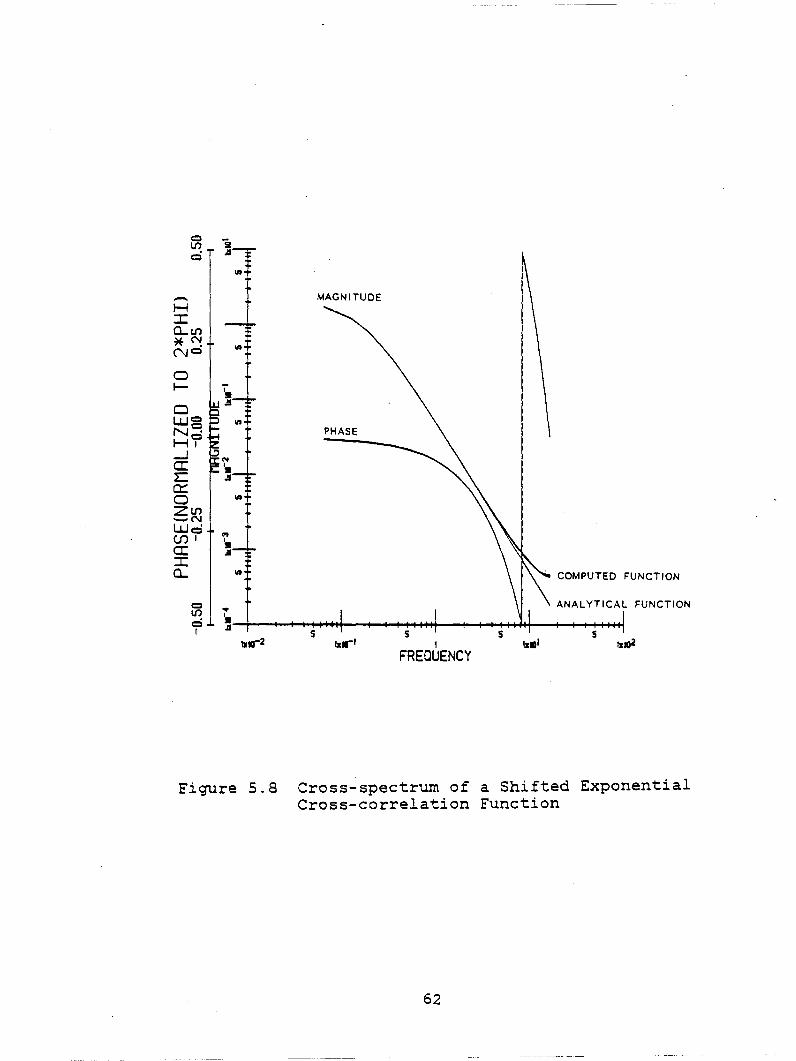
Fig. 5.8 is the cross-spectrum of a shifted exponential

cross-correlation function.

R {t) = exp(-lt-0.061) x y

The analytical cross-spectrum is almost indistinguishable

from the numerical function. The magnitudes are identical up

to near the tail end where the computed line deviates

slightly due to aliasing effect.

Fig. 5.9 is the autocorrelation function of actual

single-phase turbulence data and Fig. 5.10 is the

cross-correlation function of a pair of single-phase

turbulence data, one shifted by 0.008 second from the ether.

Note that the peak of the plot is slightly shifted from the

orgin towards the left. Cross-correlation functions can be

used to study the bubble convection from one sensor to ether

with a three-sensor probe.

The power spectrum of the single-phase liquid

turbulence data as shown on Fig. 5.11 exhibits the well

known slope of -5/3 in the inertial range. In contrast, the

power spectrum for the bubbly flow, as shown on Fig. 5.12 ,

exhibits a slope of -2.6, which is the same as reported by

Lance [8].

It appears that the spectral analysis code POWER is

running correctly and gives good estimates of

61

--------------

Q l/)

d

MAGNITUDE H ::J: Cl,. li)

*'""'! ("\JCI

0 1-

a Li.JCI "' N~ PHASE H? _J ... a: 's !: .!1

0:: 0 "' zl/) -N Li.Jd ... (./) 1 '5I a: .Il ::J: Cl.. "' COMPUTED FUNCTION

Cl • ANAL YTICAL FUNCTION l/)

'5I d .!1 1 s s tJtr2 br tri t till' tJ..Z

FREQUENCY

Figure 5.8 Cross-spectrurn of a Shifted Exponential Cross-correlation Function

62

TCSl

Figure 5.9 Autocorrelation Function of Single-phase Data

63

= (C

ci

f8 ci 1

~~------~----~------~------~----~ 1 -{).20 -{).12 -{).04 0.04 0.12 0.20

T(S)

Figure 5.10 Cross-correlation Function for A Pair of Shifted Single-phase Data

64

VI ........ .. .. E u -

s

SLOPE = -5/3

s,_. s

FREQUENCY(1/Sl

Figure 5.11 Power Spectrum of Single-phase Data

65

•

s s s 11.Z 11atl

s

FREOUENCYU/Sl

Figure 5.12 Power Spectrum of Two-phase Data

66

autocorrelation function, cross-correlation function, power

spectral function, and cross-spectral function. Furtherrnore,

when the code was run on our prelirninary data for both sin­

gle and two-phase turbulent flow, the result agreed with the

existing results.

67

CHAPTER 6

SUMMARY AND CONCLUSIONS

An airjwater loop and ether experimental apparatus have

been prepared to calibrate the single-sensor hot film

anemometer and to measure the two-phase turbulent flow. The

electrical testing of the anemometer indicates that its

frequency response stays constant up to about 29 kHz in

single-phase turbulent flow.

A data acquisiton system consisting of a 14-channel FM

tape recorder, a 4-channel A/D converter in a HP computer,

and a IBM 3033 computer was established and its capability

to digitize two simultaneous signals at a rate in excess of

10 kHz was demonstrated.

Computer codes to process the digital data from either

a single-sensor or a three-sensor anemometer were developed

and tested aginst both actual data and hypothetical data. A

new method based on the slope thresholding with level

testing was used for phase determination. The spectral

analysis code was also implemented and was found to be work­

ing correctly.

68

REFERENCES

1. Maher I. Kelada, Application of Anemometry in Two Phase Flow For Local Measurements and For the Study of Flow Behavior in The Entrance Region of a Long Vertical Pipe, Master's Thesis, University of Houston, 1977.

2. D.A. Drew and R.T. Lahey, Jr., "Phase Distribution Mechanisms in Turbulent Two-Phase Flow in Channels of Arbitrary Cross Section", J. of Fluids Engineering, Dec 1981, Vol 103.

3. Leroy M. Fingerson and Peter Freymuth, Thermal Anemometers, 1979 TSI INCORPORATED.

4. J.M. Delhaye, ''Hot-Film Anemometry in Two-Phase Flow," Froc. Eleventh National ASME/AlChe Heat Transfer Conference, Minneapolis, Minnesota, p.S8, 1969.

S. F.J. Resch, "Use of the Dual-sensor Hot-film Probe in Water Flow," DISA Information No.27, Jan. 1982.

6. Julius S. Bendat and Allan G. Piersol, Random Data: Analysis and Measurement Precedures, Wiley-Interscience, New York, 1971.

7. Alan V. Oppenheim and Ronald W. Shafer, Digital Signal Processing, Prentice-Hall Inc., Englewood Cliffs, 1975.

8. M. Lance, Contribution A L'Etude De La Turbulence Dans La Phase Liquide Des Ecoulements A Bulles, Ph.D. Thesis, L'Universite Claude Bernard De Lyon, 1979.

9. J.O. Hinze, Turbulence, 2nd ed., McGraw-Hill, Inc., 1975.

69

APPENDIX-A

LONGITUDINAL TURBULENCE LENGTH SCALES

The Integral Scale of Turbulence,Af:

Consider the longitudinal correlation coefficient de-

fined by

f(~) = u(z)u(z+~)/UZ

~~-b u(z+~)

~

L u(z)

(A. 1)

1 u

The integral scale,Af , which is a measure of the logest

connection, or correlation distance, between the velocities

at two points of the flow field is defined by [9] ,

(A. 2)

If U >> u 2 , the fluctuation at a fixed point may be imagined

to be caused by the whole turbulent flow field passing that

point as a "frozen" field. That is,

a at

- a =- u­az

70

(A. 3)

--- ---------------------------

When above condition is met(Taylor's Hypothesis), there ex-

ists a direct relationship between the longitudinal

correlation coefficient and the auto correlation function.

That is,

f(~) = R (t)/R (0) u u (A. 4)

where

~ = u '!

Substituting equation (A.4) into equation (A.2) yields

-Af = U/Ru(O)! Ru(t) dt (5.22)

0

The Dissipation Scale, Àf

! u(z) r u

If the flow is homogeneous along the mean flow direction,

then,

or,

u(z)u(z+~) = u(z-;)u(z)

u(z) au(z+~) a.t = u(z-;) au(z)

az

71

(A. 5)

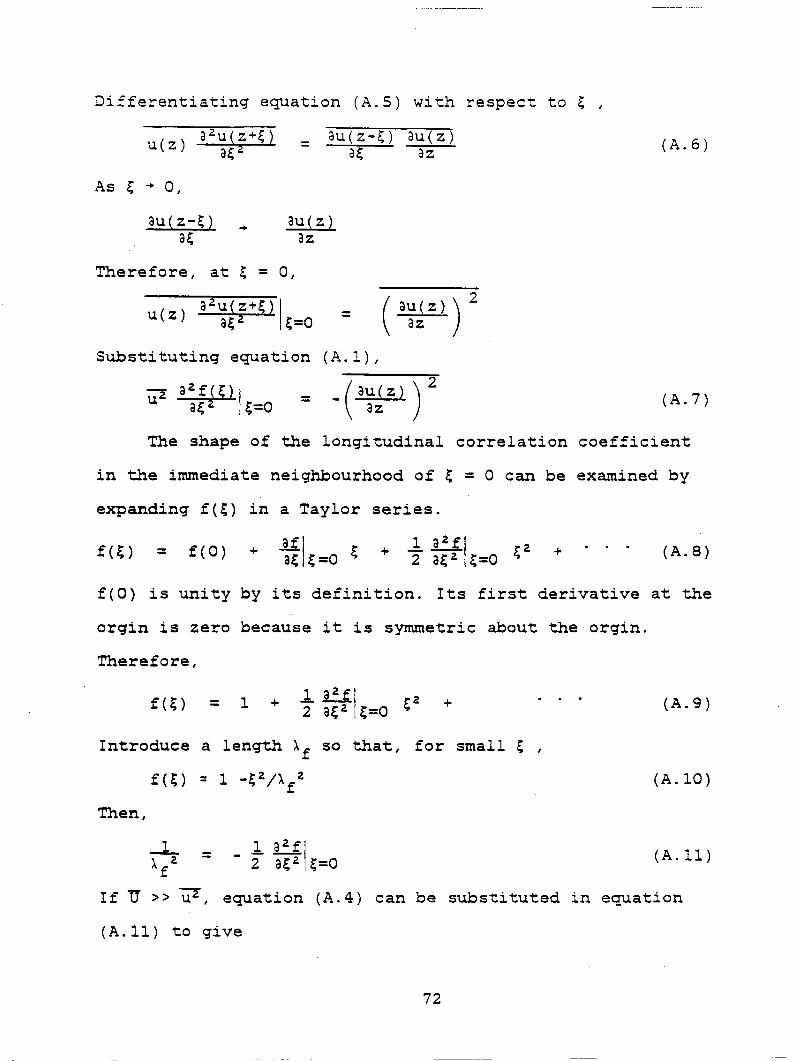
Differentiating equation (A.S) with respect to ~ 1

As ~ ...,. 0 1

au( z-q aE;

= au(z-~) au(z)

au( z) az

aE; az

Thereforel at ~ = 0 1

u(z) a'u(z+$) 1 = aE; z ~=O

Substituting equation (A.l) 1

(A. 6)

(A. 7)

The shape of the longitudinal correlation coefficient

in the immediate neighbourhood of $ = 0 can be examined by

expanding f($) in a Taylor series.

f($) = f(O) + + (A. 8)

f(O) is unity by its definition. Its first derivative at the

orgin is zero because it is symmetric about the orgin.

Thereforel

f($) = 1 + +

Introduce a length Àf so that 1 for small ~ 1

f(~) = 1 -$ 2 /Àf 2

Then,

-L À 2

f = 1 a'fj

- 2 a~ 2 ~=O

(A. 9)

(A.lO)

(A.ll)

If U >> UZI equation (A.4) can be substituted in equation

(A.ll) to give

72

--------------

1 \'2

f

1 - - _2_R_(....:;O;_)"""U,.,..2

u

- -- ----- -- - --

(5.23)

Equation (5.23) can be used to determine Àf from the

autocorrelation function of a single-phase flow. To see the

physical significance of Àf substitute equation (A.7) in

equation (A.11). Then,

1 (au) 2

= -uz az (A. 12)

side of equation (A.l2), (au;az) 2 , is the mean

square of the rate of local changes of u. We may imagine

that this local changes in u is caused by the smalles~

eddies present in the turbulent flow field. Then Àf may be

considered a measure of the average dimension of the

smallest eddies. Since smallest eddies are mainly

responsible for dissipation of kinetic energy of the flow

field into beat, Àf is called the "dissipation scale".

73

APPENDIX-B

USING DISCRETE FOURIER TRANSFORM FOR CORRELATION ESTIMATES

The discrete Fourier transform(DFT) is a Fourier repre-

sentation of a finite length sequence which is itself a se-

quence rather than a continuous function. Consider a finite

length sequence x(n) of length N. A Fourier transform pair

can be defined by,

N-1

DFT[x(n)] = X(k) = ~ x(n)exp(-j2~nk(N) , 0 ~ k ~ N-1

n=O (B.1)

and,

N-1

IDFT[X(k)] = x(n) = ~ X(k)exp(j2~nk/N) , 0 ~ n ~ N-1.

n=O (B. 2)

One property of DFT is that the inverse discrete

Fourier transform(IDFT) of the product X1 (k)Xa(k) gives the

circular convolution of x 1 (n) with x,(n). That is,

N-1

IDFT[X 1 (k)X2 (k)] = ~ x 1 (m)xa (n-m)

m=O

(B.3)

where x1 (m) is an infinite periodic sequence of period N

whose first period is identical to x 1 (n). The circular

convolution of two sequences of length 4 is illustrated in

Fig. B.l.

74

y(n) x(n)

l l 0 2 3 0 2

y{n)

-3 -2 -1 0 2 3 4 5

x(-n)

1 1 1 l 0

-1 0 2 3 4 5

CIRCULAR CONVOLUTlON OF x(n) WITH y(n)

0 2 3

Figure B.l 4-Point Circular Convolution of Two Sequences

75

The key to understanding how DFT can be used to compute

Rxy(m) is to observe that Rxy(m) is a discrete convolution

of x(-n) and y(n). For finite length sequences x(n) and

* y(n), IDFT[X (k)Y(k)] gives the circular convolution of

x(-n) and y(n). To correct for this circular effect, we have

to devise a procedure in which the input sequences are

segmented and augmented with zeros so that the circular

convolution has the effect of a linear convolution. The fol-

lowing steps computes Rxy(n) ,0 s n s L, where x(n) and y(n)

are of length N, and N is divisible by L.

( 1 ) For i

(la)

= 1, 21 ... 1 N/L - 1

Form the sequences of length 2L

x(n+(i-l)L) 1 0 s n s L-1

x 1 (n) =

0 1 L S n s 2L-l

y. (n) = y(n+(i-l)L) 1 0 sn s 2L-l ~

(lb) Compute the 2L-point DFT

2L-l

X1 (k) = 2: x 1 (n)exp(-j'Trkn/L) 1 k::i:O,l, ... I2L-l

n=O

2L-l

=2: n=O

y. (n)exp(-j'Trkn/L) , k=O,l, ... ,2L-l ~

76

* (le) Compute the 2L-point IDFT of X. (k)Y. (k) J. J.

c. (n) = J.

1 2L

2L-1

L n=O

(2) Average over c. (n) J.

R ( n) x y = 1 L(N/L - 1)

N/L - 1

L i=l

C. (n) J.

1 n=O 1 ••• 1 2L-1

n=O, ... 1 L

Note that only the first L+1 enteries of c.(n) corresponds J.

to linear convolution 1 hence retained 1 and the last L-1

entries are discarded becuase they are affected by the

cirç:ular effect.

When Fast Fourier Transforrn is used to irnplernent above

DFT 1 cornputing tirne reduction of 95% in estirnating

correlation functions is achieved.

77

APPENDIX-C

HOW TO READ THE HP PRODUCED MAGNETIC TAPE WITH THE IBM

COMPUTER

Analog signal from the anemometer was first recorded on

a FM recorder. The tape was then taken to HP computer to be

played back, digitized, and the result written on a magnetic

tape. Since the data was processed by a IBM 3033 computer, a

problem arose in reading HP produced magnetic tape with the

IBM 3033 computer at RPI.

HP computer writes the magnetic tape using "ADC

Throughput" format in which records of unspecified length

are written consecutively with inter-record gaps(IRG) but

with no end-of-file(EOF) mark. These records can be

classified as either header record or data record. A single

digitization run produces a header record followed by sever-

al data records. A typical magnetic tape has following

contents:

D 1~ D D \rj H \Ij D ~ Record: l 2 3 4 5 6

where,

H - Header record

I - Inter-record gap

D - Data record

78

The header record contains such informations as the

number of channels, the record length, the number of

records, and the digitization rate. Before each digitization

run, the operator sets these sampling parameters. The header

record consists of 44 16-bit words. Among 44 words, those

words pertinent to the sampling parameters are summarized in

Table C.l.

Each data record consists of a sequence of 16-bit data

words. The actual digital data is stored in the first 12

bits of each data word in 2's complementary form, the most

significant bit being the sign bit. The lease significant 3

bits determines the overload voltage, the voltage corre-

sponding to the full scale indicated by a 0 sign bit and all

1's in the data. The content of data word is shown on Fig.

C.l.

The digital representation is slightly shifted such

that 0 volt has equal probability of producing 0 and -1 on

the data word. The relationship between the analog signal

and the corresponding di~ital representation in the data

word is illustrated in Fig. C.2. The analog signal can be

recovered from the digital data through the following

relationship,

Voltage = (Digital data + 0.5) x Overload Voltage 2047.5

79

( c. 1)

AOC THROUGHPUT HEADER FORMAT

Word Contant

4 F~uency Code

5 Black Si:z:e

6 Number af Channels

7 Numeer af Records

a Record Langth = Number af Channels x Black Si:z:e

FREQUENCY CODES

Freq. Fmu ~~ Freq. ~~ T Code (MAX FREQ) (.0. TlME} CQde (~ FR!Q) (TOTAL TlME)

~7 100kHz s .... 56 1000Hz 1maec ~:J 50kHz 10,....: 52 500Hz 2nuec :m 21; kHz 20...-: 63 200Hz SmMC 48 10kHz 50 ...... 59 100Hz IOmMC ~2 5kHz 100 lloiMlC !'15 r.o Hz "lOnwc :Ill 2.:; kHz 200 I'OICIC 62 20 lfz 50miH!C ~5 1kHz i.>OO ...... ..: 511 10Hz 100-~1.8 .5kHz 1000 ~JoNC 54 5tn 200maoec :17.4 .25kHz 2000 .. - 61 2Hz 500ruec :13,15 0.1 kHz sooo...- 57,24 1Hz IOOOtnaae

S3,20 .5Hz 2000mMC 49,31 .2Hz 5000maac

Il 110Hz 10m.- 27 100 mHz 10MC 7 25Hz 20INIIIC 2:l r.o mHz 20scc 14 10Hz 50...- JO 20 mHz r.o-10 S Hz IOOINIIIC 26 10 mHz 100 MC

6 2.5Hz 200maec 22 SmHz 200MC 13 !Hz 500maec 29 2mHz 500aec 9 0.5 Hz IOOOmaec 25 1 mHz IOOOMC 5 0.25 Hz 2000- 21 0.5mHz 2000aec 1 0.1 Hz 5000- 17 0.2mHz 5000aec:

Table II AOC Throughput Header Content

80

bit no. 15 14 13 12 1 1 10 9 8 7 6 5 4 3 2 0

ri 1 1 1 1 1 1 1 1 1 1 1 1 1 1 1 1

to=J~ sign 0 = + DATA 1 = -

bit 3 set = this data word be displayed in REPEAT mode.

OVERLOAD VOLTAGE switch setting

0 = +8 volts 4 = •o. 12s volt 1 = +4 volts 5 = +0.25 volt 2 = +2 volts 6 = +0.5 volt 3 = ., volt

Figure C.l Data Word Content

81

204 7 1 1 1 1 1 1 1 1 1 1 1 1 1 1 1 1 1 1 1 1 1 1 1 1 1

o 1 o!ololol olol@ ololololol -1 ,~-=,..,..1 ':"'"11 I-:'1"'T"'i:-T 11-:'1..,...1 ':"'"11 1:-:-. 1-:-1 ,~l-.,..1 ..,-1 1....,..1-1 ..-1 1....,1

-2 1 1 Il( 1 1 11 1/1/11 1 1 1 1 1 1 1 1 o 1

-2048 l1lololololotololol ololol

1. OVERLOAD VOLTAGE

...,......

.:.,-------- 0

- OVERLOAD VOLTAGE

Figure C.2 Schematic of the Relationship Between The Analog Signal and The Corresponding Digital Representation in The Data Word

82

Reading the magnetic tape and manipulating bits to

recover the data was implemented using FORTRAN statements.

Since the IBM computer has 32-bit word architecture,

half-word integer array was used to read in the data

records. Because the digital data in the data words is not

in ASCII code, the data records were read using character

data format, not integer. Then, the least significant 4 bits

of each data word were removed by dividing each integer

array by 16. If the result came out negative, one was

subtracted from the result. Lastly, the actual signal was

recovered by equation (C.l) In practice the header record

and the first three bits of each data word were not read ex­

cept for checking purpose because we know these sampling pa­

rameters beforehand.

83

APPENDIX-D

COMPUTER PROGRAM LISTING

84

C SUBROUTINE VOIDl c C SUBPROGRAM TO PROCESS DIGITIZED DATA FROM SINGLE CHANNEL HOT FILM C ANEMOMETER IN TWO PHASE FLOW. FLOW PARAMETERS BEING COMPUTED ARE C LIQUID PHASE MEAN VELOCITY, ITS TURBULENCE INTENSITY, AND THE VOID C FRACTION. TO SEPARATE GAS PHASE SIGNALS, COMBINATION OF SLOPE C AND LEVEL THRESHOLDING IS USED. BESIDE THE FLOW PARAMETERS THIS C SUBPROGRAM OUTPUTS SEVERAL STATISTICS TO MONITOR WORKING OF THE C ALGORITHM. c c-----------------------------------------------------------------------c C INPUT ARGUMENTS c C NORCRD - NUMBER OF DATA RECORDS C GSCALE - SCALE FACTOR OF THE DIGITIZED DATA C GZERO - ZERO OF THE DIGITIZED DATA: VOLTAGE = GSCALE*(DATA - GZERO) C A -C B -CALIBRATION CONSTANTS: VLOTAGE**2 =A+ B*VELOCITY**(l/C) c c -C ECRITl - GAS PHASE IS INITIATED WHEN TWO CONSECUTIVE VOLTAGE INCREMENTS C ARE BOTH GREATER THAN ECRITl C ECRIT2 - MINIMUM VOLTAGE DECREMENT REQUIRED TO TERMINAlE GAS PHASE C LEVEL1 - LIQUID PHASE TERMINAlES WHEN THE SIGNAL FALLS BELOW THIS LEVEL C LEVEL2 - GAS PHASE TERMINAlES WHEN THE SIGNAL RISES ABOVE THIS LEVEL C LEAD - TIME IN UNIT OF 0.1 MSEC BETWEEN THE PROBE-INTERFACE CONTACT AND PENETRATION C DELAY - INACTIVE PERIOD IN UNIT OF 0.1 MSEC FOLLOWING THE VOIDS POSTERIAL PEAK

00 C OPTION - IF EQUAL TO 1, LOCATIONS OF ALL PAIRS OF VOIDS TOUCHING EACH ln C OTHER ARE PRINTED

c C OUTPUT ARGUMENT c C GATE - VECTOR CONTAINING THE LOCATIONS OF PHASE CHANGE C -'VE SIGN INDICATES THE PHASE CHANGE FROM LIQUID TO GAS C +'VE SIGN INDICATES THE PHASE CHANGE FROM GAS TO LIQUID c C VARIABLES USED c C N - COUNTER FOR NUMBER OF DATA POINTS PROCESSED C L - COUNTER FOR NUMBER OF DATA RECORDS PROCESSED C NOBUBL - COUNTER FOR NUMBER OF VOIDS C DOUBLE - COUNTER FOR NUMBER OF PAIRS OF VOIDS TOUCHING EACH OTHER C LTIME - COUNTER FOR THE LEAD TIME C PTIME - COUNTER FOR PASSAGE liME C GAS - COUNTER FOR NUMBER OF DATA POINTS CORRESPONDING TO GAS PHASE C LIQUID - COUNTER FOR NUMBER OF DATA POINTS CORRESPONDING TO LIQUID PHASE C G( 1) - HALF LENGTH INTEGER CONTAINING 1-TH DATA POINT IN THE RECORD CE( 1) -VOLTAGE CORRESPONDING TO G( 1) C V - VELOCITY IN CM/SEC C SUM - RUNNING SUM OF VELOCITIES

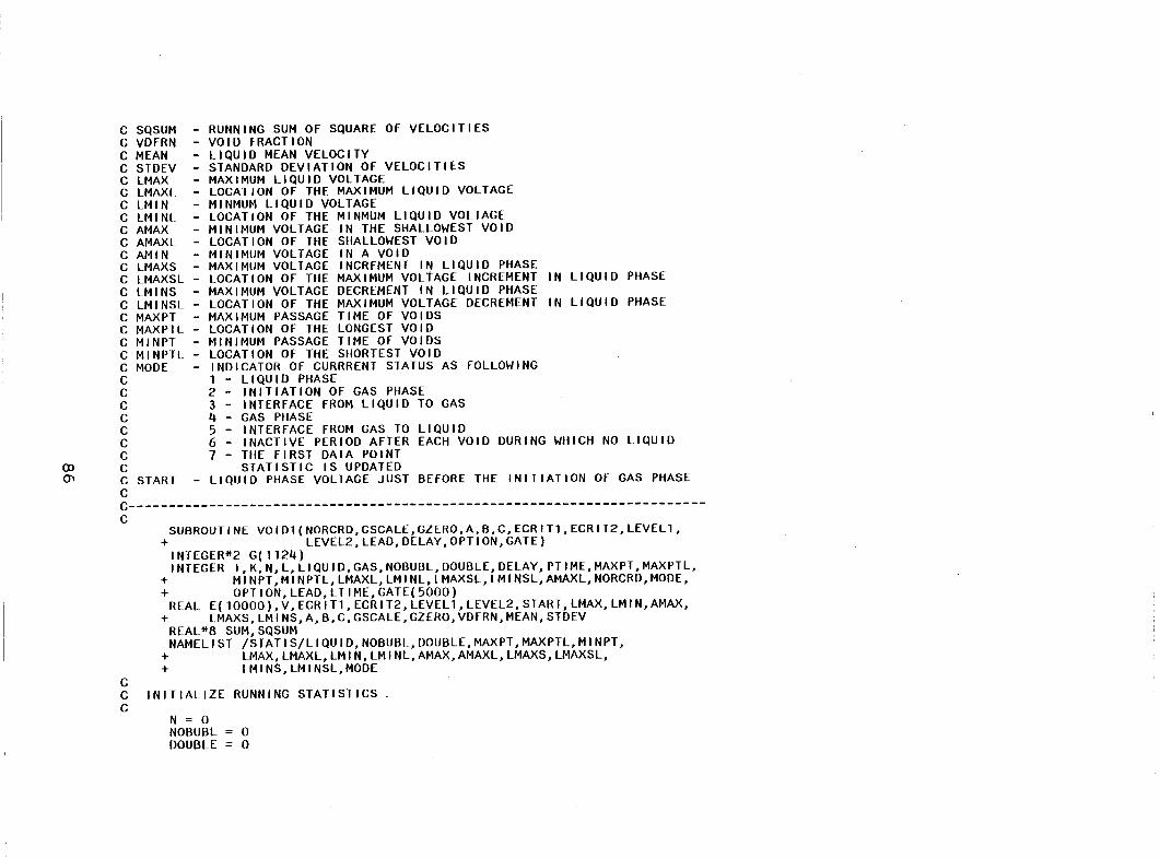
C SQSUM - RUNNING SUM Of SQUARE Of VELOCITIES C VDFRN - VOID FRACTION C MEAN - LIQUID MEAN VELOCITY C STDEV - STANDARD DEVIATION Of VELOCITIES C LMAX - MAXIMUM LIQUID VOLTAGE C LMAXL - LOCATION Of THE MAXIMUM LIQUID VOLTAGE C LMIN - MINMUM LIQUID VOLTAGE C LMINL - LOCATION Of THE MINMUM LIQUID VOLTAGE C AMAX - MINIMUM VOLTAGE IN THE SHALLOWEST VOID C AMAXL - LOCATION Of THE SHALLOWEST VOID C AMIN - MINIMUM VOLTAGE IN A VOID C LMAXS - MAXIMUM VOLTAGE INCREMENT IN LIQUID PHASE C LMAXSL - LOCATION Of THE MAXIMUM VOLTAGE INCREMENT IN LIQUID PHASE C LMINS - MAXIMUM VOLTAGE DECREMENT IN LIQUID PHASE C LMINSL - LOCATION Of THE MAXIMUM VOLTAGE DECREMENT IN LIQUID PHASE C MAXPT - MAXIMUM PASSAGE liME Of VOIDS C MAXPTL - LOCATION Of THE LONGEST VOID C MINPT - MINIMUM PASSAGE liME Of VOIDS C MINPTL - LOCATION Of THE SHORTEST VOID C MODE - INDICATOR Of CURRRENT STATUS AS FOLLOWING C 1 - LIQUID PHASE C 2 - INITIATION Of GAS PHASE C 3 - INTERFACE FROM LIQUID TO GAS C 4 - GAS PHASE C 5 - INTERFACE FROM GAS TO LIQUID C 6 - INACTIVE PERIOD AFTER EACH VOID DURING WHICH NO LIQUID C 7 - THE FIRST DATA POINT

00 C STATISTIC IS UPDATED ~ C START - LIQUID PHASE VOLTAGE JUST BEFORE THE INITIATION Of GAS PHASE

c c------------------------------------------------------------------------c

SUBROUTINE VOID1(NORCRD,GSCALE,GZERO,A,B,C,ECRIT1,ECRIT2,LEVEL1, + LEVEL2,LEAD,DELAY,OPTION,GATE)

INTEGER*2 G(1124) INTEGER I,K,N,L,LIQUID,GAS,NOBUBL,DOUBLE,DELAY,PTIME,MAXPT,MAXPTL,

+ MINPT,MINPTL,LMAXL,LMINL,LMAXSL,LMINSL,AMAXL,NORCRD,MODE, + OPTION,LEAD,LTIME,GATE(5000)

REAL E(10000),V,ECRIT1,ECRIT2,LEVEL1,LEVEL2,START,LMAX,LMIN,AMAX, + LMAXS,LMINS,A,B,C,GSCALE,GZERO,VDFRN,MEAN,STDEV

REAL*B SUM,SQSUM NAMELIST /STATIS/LIQUID,NOBUBL,DOUBLE,MAXPT,MAXPTL,MINPT,

+ LMAX,LMAXL,LMIN,LMINL,AMAX,AMAXL,LMAXS,LMAXSL, + LMINS,LMINSL,MODE

c C INITIALIZE RUNNING STATISTICS . c

N = 0 NOBUBL = 0 DOUBLE = 0

00 ....J

c

LIQU 1 D = 0 GAS = 0 SUM = O. SQSUM = O. LMAX = O. LMIN = 100. LMAXS = O. LMINS = O. MAXPT = 0 Ml NPT = 1000 AMAX = 0 LTIME = 0 If (OPTION .NE. 1) GO TO 90 WRITE(6 82)

82 FORMAT( 11','LOCATIONS OF DOUBLES') 90 CONTINUE

C SET ENTERING VALUES OF THE LOOP c

MODE = 7 K = DELAY + 1

c C PROCESS EACH DATA RECORD c

c c c

c

DO 2000 L=1,NORCRD

EACH RECORD CONTAINS 1024 DATA POINTS

READ(5,85) (G( 1 ), 1=101, 1124) 85 FORMAT(128(8A2))

C PROCESS EACH DATA POINT c

c

DO 1000 1=101,1124 G( 1 ) = G( 1 ) /16 E( 1) = GSCALE*(G( 1) + 0.5- GZERO) N = N + 1

C PROCESS THE DATA POINT ACCORDING TO CURRENT STATUS c

GO T0(100,200,300,400,500,600,70),MODE c C THE FIRST DATA POINT c

70 CONTINUE IF(E( 1) .LE. LEVELl) GO TO 80

NG = 1 GATE(NG) = LTIME = 0 MODE = 1

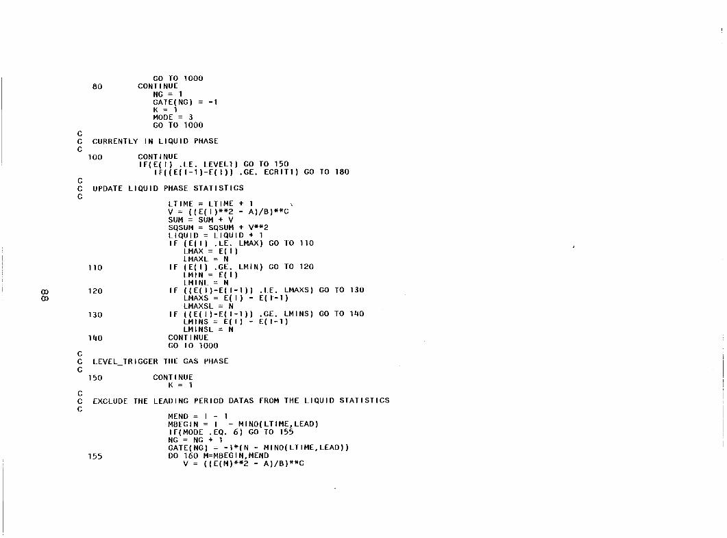
00 00

c

GO TO 1000 80 CONTINUE

NG = 1 GA TE ( NG) = -1 1< = 1 MODE = 3 GO TO 1000

C CURRENTLY IN LIQUID PHASE c

100 CONTINUE

c

IF(E( 1) .LE. LEVELl) GO TO 150 IF((E(I-1)-E(I)) .GE. ECRITl) GO TO 180

C UPDATE LIQUID PHASE STATISTICS c

110

120

130

140

c

LTIME = LTIME + 1 V= ((E( 1)**2- A)/B)**C SUM = SUM + V SQSUM = SQSUM + V**2 LIQUID = LIQUID + 1 IF (E( 1) .LE. LMAX) GO TO 110

LMAX = E( 1) LMAXL = N

1 F ( E ( 1 ) . GE. LM 1 N) GO TO 120 LMI N = E( 1) LMINL = N

IF ((E(I)-E(I-1)) .LE. LMAXS) GO TO 130 LMAXS = E ( 1 ) - E ( 1·-1 ) LMAXSL = N

IF ((E(I)-E(I-1)) .GE. LMINS) GO TO 140 LM 1 N S = E ( 1 ) - E ( 1 -1 ) LMINSL = N

CONTINUE GO TO 1000

C LEVEL TRIGGER THE GAS PHASE c -150

c

CONTINUE K = 1

C EXCLUDE THE LEADING PERIOD DATAS FROM THE LIQUID STATISTICS c

155

MEND = 1 - 1 MBEGIN = 1 - MINO(LTIME,LEAD) IF(MODE .EQ. 6) GO TO 155 NG = NG + 1 GATE(NG) = -l*(N- MINO(LTIME,LEAD)) DO 160 M=MBEGIN,MEND

V= ((E(M)**2- A)/B)**C

ro \{)

160

c

SUM = SUM - V SQSUM = SQSUM - V**2 LIQUID = LIQUID - 1 GAS = GAS + 1

CONTINUE MODE = 3 START = E( 1-1) GO TO 1000

C SLOPE TRIGGER THE GAS PHASE c -

c

180 CONTINUE MODE = 2 GO TO 1000

C CURRENTLY IN THE BEGINNING OF LIQUID TO GAS INTERFACE c

c

200 CONTINUE IF((E(I-1)-E(I)) .LT. ECRITl .AND. E(l) .GT. LEVELl)GOTO 250

START = E( 1-2) K = 2 MODE = 3

C EXCLUDE THE LEADING PERIOD DATA FROM THE LIQUID STATISTICS c

220

c

MEND = 1 - 2 MBEGIN = 1 - 1 - MINO(LTIME,LEAD) NG = NG + 1 GATE(NG) = -1*(N- 1 - MINO(LTIME,LEAD)) DO 220 M=MBEGIN,MEND

V= ((E(M)**2- A)/B)**C SUM = SUM - V SQSUM = SQSUM - V**2 LIQUID = LIQUID - 1 GAS = GAS + 1

CONTINUE LTIME = 0 GO TO 1000

C SINCE THE SECOND DECREMENT IS SMALLER THAN ECRIT1, GO BACK TO LIQUID PHASE c

250 CONTINUE DO 280 M=1,2

J = 1 - M + 1 LTIME = LTIME + 1 V= ((E(J)**2- A)/B)**C SUM = SUM + V SQSUM = SQSUM + V**2 LIQUID = LIQUID + 1 IF (E(J) .LE. LMAX) GO TO 272

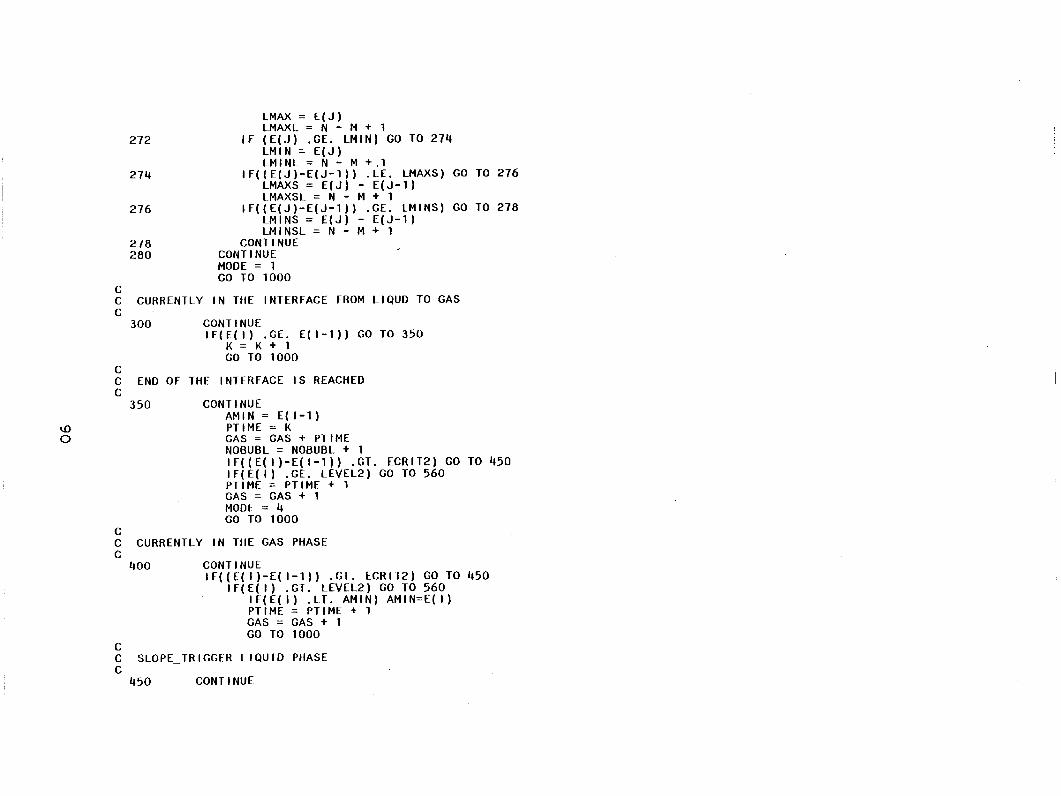
~ 0

c

272

274

276

278 280

LMAX = E( J) LMAXL = N - M + 1

If (E(J) .GE. LMIN) GO TO 274 LMI N = E(J) LMINL = N- M +.1

lf((E(J)-E(J-1)) .LE. LMAXS) GO TO 276 LMAXS = E(J) - E(J-1) LMAXSL = N - M + 1

lf((E(J)-E(J-1)) .GE. LMINS) GO TO 278 LMINS = E(J) - E(J-1) LMINSL = N - M + 1

CONTINUE CONTINUE MODE = 1 GO TO 1000

C CURRENTLY IN THE INTERFACE FROM LIQUD TO GAS c

c

300 CONTINUE IF(E(I) .GE. E(l-1)) GO TO 350

K = K + 1 GO TO 1000

C END OF THE INTERFACE IS REACHED c

350

c

CONTINUE AMIN = E( 1-1) PTIME = K GAS = GAS + PTIME NOBUBL = NOBUBL + 1 IF((E(I)-E(I-1)) .GT. ECRIT2) GO TO 450 IF(E( 1) .GE. LEVEL2) GO TO 560 PTIME = PTIME + 1 GAS = GAS + 1 MODE = 4 GO TO 1000

C CURRENTLY IN TllE GAS PHASE c

c

400 CONTINUE IF((E(I)-E(I-1)) .GT. ECRIT2) GO TO 450

IF(E( 1) .GT. LEVEL2) GO TO 560 1 f ( E ( 1 ) . l T. AM 1 N ) AM 1 N= E ( 1 ) PTIME = PTIME + 1 GAS = GAS + 1 GO TO 1000

C SLOPE TRIGGER LIQUID PHASE c -

450 CONTINUE

c

K = 1 MODE = 5 GO TO 1000

C CURRENTLY IN THE INTERFACE FROM GAS TO LIQUID PHASE c

c

500 CONTINUE lf(E(I) .LT. E(l-1)) GO TO 550

K = K + 1 GO TO 1000

C CHECK WHETHER END Of THE VOID PEAKS HIGHER THAN THE BEGINNING c

550 CONTINUE lf(E( l-1) .GT. START) GO TO 560

c C GO BACK TO THE GAS PHASE c

551

c

K = K + PTIME + 1 GAS = GAS - PTIME DOUBLE = DOUBLE + 1 If (OPTION .EQ. 1) WRITE(6,551) N FORMAT( lOX, 110) MODE = 3 GO TO 1000

C TERMINAlE THE GAS PHASE 1.0 c 1-' 560 CONTINUE

If (PTIME .LE. MAXPT) GO TO 562 MAXPT = PTIME MAXPTL = N

562 If (PTIME .GE. MINPT) GO TO 564 MINPT =PTIME MINPTL = N

564 If (AMIN .LE. AMAX) GO TO 566 AMAX = AMIN AMAXL = N

566 CONTINUE K = 1 MODE = 6 GO TO 1000

c C CURRENTLY IN THE DELAY PERIOD c

600 CONTINUE K = K + 1 If (K .GT. DELAY) GO TO 650

1 f ( E( 1 ) . LE. LEVELl) GO TO 150 GO TO 1000

U> N

c C DELAY TERMINATED. START TO UPDATE LIQUID STATISTICS c

650

1000 c

CONTINUE LTIME = 0 MODE = 1 NG = NG + 1 GATE(NG) = N + 1 GO TO 1000

CONTINUE

c PREPARE TO READ IN THE NEXT DATA RECORD c

1500 2000

c

DO 1500 1=1, 100 E(l) = E(1024+1)

CONTINUE CONTINUE

c CALCULATE TWO PHASE FLOW PARAMETERS c

c

MEAN = SUM/LIQUID STDEV = DSQRT(SQSUM/LIQUID- MEAN**2) VDFRN = FLOAT(GAS)/N

C PRINT OUT THE FLOW PARAMETERS AND THE STATISTICS c

2100

2200

2300

2400

WRITE(6,2100) MEAN FORMAT(1X,'MEAN AXIAL LIQUID VELOCITY IS ',F6.3, 1 CM/SEC') WRITE(6,2200) STDEV FORMAT(1X, 'STANDARD DEVIATION OF THE VELOCITY IS ',F6.3, 'CM/SEC') WRITE(6,2300) VDFRN FORMAT(lX,'VOID FRACTION IS 1 ,F6.5) WRITE(6 12400) FORMAT( O', 1

')

WRITE(6,STATIS) NG = NG + 1 GATE(NG) = 0 RETURN END

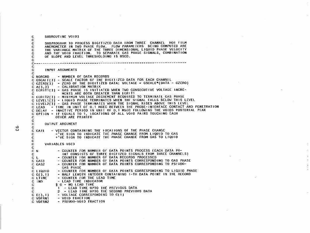
C SUBROUTINE VOID3 c C SUBPROGRAM TO PROCESS DIGITIZED DATA FROM THREE CHANNEL HOT FILM C ANEMOMETER IN TWO PHASE FLOW. FLOW PARAMETERS BEING COMPUTED ARE C TlfE VARIANCE MATRIX Of TlfE TlfREE DIMENSIONAL LIQUID PHASE VELOCITY C AND TIIE VOID FRACTION. TO SEPARATE GAS PlfASE SIGNALS, COMBINATION C Of SLOPE AND LEVEL TlfRESifOLDING IS USED. c c--------------------------------~--------------------------------------c C INPUT ARGUMENTS c C NORCRD - NUMBER Of DATA RECORDS C GSCALE(3) - SCALE FACTOR Of TlfE DIGITIZED DATA FOR EACif CHANNEL C GZER0(3) - ZERO Of THE DIGITIZED DATA: VOLTAGE= GSCALE*(DATA- GZERO) C A(3,3) - CALIBRATION MATRIX C ECRIT1(3) - GAS PlfASE IS INITIATED WlfEN TWO CONSECUTIVE VOLTAGE INCRE-e MENTS ARE BOTH GREATER TlfAN ECRIT1 C ECRIT2(3) -MINIMUM VOLTAGE DECREMENT REQUIRED TO TERMINAlE GAS PHASE C LEVEL1(3) - LIQUID PlfASE TERMINAlES WHEN TlfE SIGNAL FALLS BELOW TlfiS LEVEL C LEVEL2(3) - GAS PlfASE TERMINAlES WHEN TlfE SIGNAL RISES ABOVE TlfiS LEVEL C LEAD - TIME IN UNIT Of 0.1 MSEC BETWEEN THE PROBE-INTERFACE CONTACT AND PENETRATION C DELAY - INACTIVE PERIOD IN UNIT Of 0.1 MSEC FOLLOWING TlfE VOIDS POSTERIAL PEAK C OPTION - If EQUALS TO 1, LOCATIONS Of ALL VOID PAIRS TOUCHING EACif C OTifER ARE PRINTED c C OUTPUT ARGUMENT

~ c W C GATE - VECTOR CONTAINING THE LOCATIONS OF TlfE PifAS[ CHANGE

C -'VE SIGN TO INDICATE TlfE PHASE CHANGE FROM LIQUID TO GAS C +'VE SIGN TO INDICATE THE PHASE CHANGE FROM GAS TO LIQUID c C VARIABLES USED c C N - COUNTER FOR NUMBER Of DATA POINTS PROCESS (EACif DATA PO-e INT CONSISTS Of TlfREE DIGTIZED SIGNALS FROM TlfREE CHANNELS) C L - COUNTER FOR NUMBER Of DATA RECORDS PROCESSED C GAS1 - COUNTER FOR NUMBER Of DATA POINTS CORRESPONDING TO GAS PHASE C GAS2 - COUNTER FOR NUMBER Of DATA POINTS CORRESPONDING TO PSEUDO-C GAS PlfASE C LIQUID - COUNTER FOR NUMBER Of DATA POINTS CORRESPONDING TO LIQUID PHASE C G(3, 1) - lfALF LENGTif INTEGER CONTAINING 1-Tif DATA POINT IN THE RECORD C LTIME - COUNTER FOR THE LEAD TIME C IND - LEAD TIME INDICATOR C § 0 - NO LEAD TIME C 1 - LEAD TIME UPTO TlfE PREVIOUS DATA C 2 - LEAD TIME UPTO TlfE SECOND PREVIOUS DATA C E(3, 1) -VOLTAGE CORRESPONDING TO G( 1) C VDFRN1 - VOID FRACTION C VDFRN2 - PSEUDO-VOID FRACTION

c c c c c c c c c c c c

EMEAN(3) EVAR(3,3) VVAR(3,3) TEMP(3,3) MODE(3)

C START(3) c

- MEAN VECTOR Of THE VOLTAGES - VARIANCE MATRIX Of THE VOLTAGES - VARIANCE MATRIX OF THE VOLTAGES - TEMPORARY STORAGE SPACES - INDICATOR Of CURRRENT STATUS AS

1 - LIQUID PHASE 2 - INITIATION Of GAS PHASE 3 - INTERFACE FROM LIQUID TO GAS 4 - GAS PHASE 5 - INTERFACE FROM GAS TO LIQUID 6 - INACTIVE PERIOD AfTER EACH VOID

STATISTIC IS UPDATED - LIQUID PHASE VOLTAGE JUSt BEFORE

FOLLOWING

DURING WHICH NO LIQUID

THE INITIATION Of GAS PHASE

c------------------------------------------------------------------------c SUBROUTINE VOID3(NORCRD,GSCALE,GZERO,A,ECRIT1,ECRIT2,LEVEL1,

+ LEVEL2,LEAD,DELAY,OPTION,GATE) INTEGER*2 G(3,1124) INTEGER R,N,L,LIQUID,GAS1,GAS2,DELAY,NORCRD,MODE(3),0PTION

+ , 11, 12,K(3),LEAD,LTIME, IND,FLAG,GATE(5000) REAL E(3,10000),ECRIT1(3),ECRIT2(3),LEVEL1(3),LEVEL2(3),START(3),

+ A(3,3),GSCALE(3),GZER0(3),VDfRN1,VDfRN2,VVAR(3,3),TEMP(3,3) REAL*8 EMEAN(3),EVAR(3,3) LOGICAL LPHASE(3),GPHASE(3)

c C INITIALIZE RUNNING STATISTICS

1.0 c .P. N=O

c

LIQU 1 D = 0 GAS1 = 0 GAS2 = 0 IND = 0 fLAG = 0 LT IME = 0 GATE(1) = NG = 1 DO 50 1=1,3

MODE( 1) = 6 K( 1 ) = DELAY + 1 DO 45 J=1,3

EVAR( I,J) =O. VV AR ( 1 , J ) = 0. TEMP(I,J) =O.

1t5 CONT 1 NUE 50 CONTINUE

C PROCESS EACH DATA RECORD c

DO 2000 L=l,NORCRD

\0 U1

c C EACH RECORD CONTAINS 1024 SETS Of DATA POINTS c

READ(5,85)(G( 1,1 ),1=101,1124) 85 FORMAT(128(8A2))

c C PROCESS EACH DATA POINT c

c

DO 1000 1=101,1124 N = N + 1 G(2,1) = G(1,1) G( 3, 1) = G( 1, 1) DO 900 R=1,3

LPHASE(R) = .FALSE. GPHASE(R) = .FALSE. G(R,I) = G(R,I )/16 E(R,I) = GSCALE(R)*(G(R,I) + 0.5- GZERO(R))

C PROCESS THE DATA POINT ACCORDING TO CURRENT STATUS c

MD = MODE(R) GO T0(100,200,300,400,500,600),MD

c C CURRENTLV IN LJQUJD PHASE c

100

c

CONTINUE lf((E(R,I-1)-E(R,I)) .GE. ECRITl(R)) GO TO 180

lf(E(R,I) .LE. lEVEll(R)) GO TO 150 LPHASE(R) = .TRUE. GO TO 900

C lEVEl TRIGGER THE GAS PHASE c -150

c

CONTINUE MODE(R) = 3 If (flAG .EQ. 0) IND = GPHASE(R) = .TRUE. START(R) = E(R, 1-1) GO TO 900

C SLOPE TRJGGER THE GAS PHASE c -

c

180 CONTINUE MODE(R) = 2 GPHASE(R) = .TRUE. GO TO 900

C CURRENTLV IN THE BEGINNING Of LIQUID TO GAS INTERFACE c

200 CONTINUE

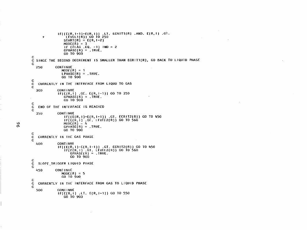
1.0 (}'\

c

IF((E(R,I-1)-E(R,I)) .LT. ECRITl(R) .AND. E(R,I) .GT. + LEVEL1(R)) GO TO 250

START(R) = E(R,I-2) MODE(R) = 3 IF (FLAG .EQ. -1) IND = 2 GPHASE(R) = .TRUE. GO TO 900

C SINCE THE SECOND DECREMENT IS SMALLER THAN ECRIT1(R), GO BACK TO LIQUIO PHASE c

250

c

CONTINUE MODE(R) = LPHASE(R) GO TO 900

. TRUE.

C CURRENTLY IN THE INTERFACE FROM LIQUD TO GAS c

c

300 CONTINUE IF(E(R,I) .GE. E(R,I-1)) GO TO 350

GPHASE(R) = .TRUE. GO TO 900

C END OF THE INTERFACE IS REACHED c

350

c

CONTINUE IF((E(R,I)-E(R,I-1)) .GT. ECRIT2(R)) GO TO 450 IF(E(R,I) .GE. LEVEL2(R)) GO TO 560 MODE(R) = 4 GPHASE(R) = .TRUE. GO TO 900

C CURRENTLY IN THE GAS PHASE c

c

400 CONTINUE IF((E(R,I)-E(R,I-1)) .GT. ECRIT2(R)) GO TO 450

1 F( E( R. 1) • GT. LEVEL2( R)) GO TO 560 GPHASE(R) = .TRUE. GO TO 900

C SLOPE TRIGGER LIQUID PHASE c -

c

450 CONTINUE MODE(R) = 5 GO TO 900

C CURRENTLY IN THE INTERFACE FROM GAS TO LIQUID PHASE c

500 CONTINUE IF(E(R,I) .LT. E(R,I-1)) GO TO 550

GO TO 900

\{) -....]

c C CHECK WHETHER END Of THE VOID PEAKS HIGHER THAN THE BEGINNING c

550 CONTINUE lf(E(R, l-1) .GT. START(R)) GO TO 560

c C GO BACK TO THE GAS PHASE c

c c c

c c c

c c c

c

551 552

If (OPTION .NE. 1) GO TO 552 LT = R*l.E6 + N WRITE(6,551) LT FORMAT( 10X, 110)

CONTINUE MODE(R) = 3 GPHASE(R) = .TRUE. GO TO 900

TERMINAlE THE GAS PHASE

560 CONTINUE K( R) = 1 MODE(R) = 6 GO TO 900

CURRENTLY IN THE DELAY PERIOD

600 CONTINUE K(R) = K(R) + 1 If (K(R) .GT. DELAY) GO TO 650

If (E(R,I) .LE. LEVELl(R)) GO TO 630 GO TO 900

LEVEL_TRIGGER THE GAS PHASE

630 CONTINUE K( R) = 1 MODE(R) = 3 GPHASE(R) = .TRUE. GO TO 900

C DELAY TERMINATED. START TO UPDATE LIQUID STATISTICS c

c

650 CONTINUE MODE(R) = GO TO 900

900 CONTINUE

C EXCLUDE THE LEADING PERIOD DATA FROM THE LIQUID PHASE STATISTICS c

If( INO .EQ. 0) GO TO 909

c

MEND = 1 - IND MBEGIN = 1 - IND- MINO(LTIME,LEAD) + 1 DO 908 M=MBEGIN,MEND

LIQUID = LIQUID - 1 GAS1 = GAS1 + 1 DO 907 11=1,3

EMEAN( 11 ) = EMEAN( 11) - E( 11, M) DO 906 12=1,3

EVAR( 11,12) = EVAR( 11,12) - E( 11,M)*E( 12,M) 906 CONTINUE 907 CONTINUE 908 CONTINUE

IND = 0 GO TO 950

C If ALL THREE SENSORS ARE IN LIQUID, UPDATE THE MEAN AND VARIANCE c

909 If( .NOT. LPHASE(1) .OR .. NOT. LPHASE(2) .OR .. NOT. + LPHASE(3)) GO TO 940

fLAG = 0 LIQUID = LIQUID + 1 LTIME = LTIME + 1 DO 910 11=1,3

EMEAN(11) = EMEAN(I1) + E(l1,1) DO 91 5 1 2= 1 , 3

EVAR(I1,12) = EVAR(I1,12) + E(11,1)*E(I2,1) 915 CONTINUE

~ 910 CONTINUE 00 lf(GATE(NG) .GT. 0) GO TO 1000

NG = NG + 1 GATE(NG) = N GO TO 1000

c C If ALL THREE SENSORS ARE IN GAS, INCREMENT THE NUMBER Of VOIDS c

940

950

980

1000 c

+

+

lf(GATE(NG) .LT. 0) GO TO 950 NG = NG + 1 GATE(NG) = -1*N fLAG = fLAG - 1 lf(fLAG .NE. -1) LTIME = 0 lf(.NOT. GPHASE(1) .OR .. NOT. GPHASE(2) .OR .. NOT.

GPHASE(3)) GO TO 980 GAS1 = GAS1 + 1 GO TO 1000

If( .NOT. GPHASE(1) .AND .. NOT. GPHASE(2) .AND .. NOT. GPHASE(3)) GO TO 1000 GAS2 = GAS2 + 1

CONTINUE

c PREPARE TO READ IN THE NEXT DATA RECORD

c

c

1300 1500 2000

DO 1500 1=1,100 DO 1300 J=1,3

E(J,I) = E(J,1024+1) .CONTINUE

CONTINUE CONTINUE

C COMPUTE THE VOID fRACTION c

c

VDFRNl = fLOAT(GASl)/N VDFRN2 = FLOAT(GAS2)/N

C COMPUTE THE MEAN AND VARIANCE Of THE VOLTAGE READINGS c

DO 2100 11=1,3 EMEAN( 11) = EMEAN( 11)/LIQUID DO 2200 12=1,3

2200 2100

c

EVAR( 11, 12) = EVAR( 11, 12)/LIQUID CONTINUE

CONTINUE

DO 2300 11=1,3 DO 2400 12=1,3

EVAR(I1,12) = EVAR(I1,12)- EMEAN(Il)*EMEAN(12) 2400 CONTINUE 2300 CONTINUE

\!) c \0 C RELATE THE VOLTAGE VARIANCE TO THE VELOCITY VARIANCE

c

c

c

2700 2600 2500

DO 2500 11=1,3 DO 2600 12=1,3

DO 2700 13=1,3 TEMP( 11, 12)

CONTINUE CONTINUE

CONTINUE

DO 2800 1 1 = 1 , 3 DO 2900 12=1,3

DO 3000 13=1,3

EVAR( 11, 13)*A( 12, 13) + TEMP( 11, 12)

VVAR( 11, 12) = VVAR( 11, 12) +A( 11, 13)*TEMP( 13, 12) 3000 CONTINUE 2900 CONTINUE 2800 CONTINUE

C PRINT OUT THE RESULTS c

WRITE(6 3100) VDFRN1 3100 FORMAT('O','VOID FRACTION IS ',f6.5)

l-' 0 0

WRITE(6,3200) VDFRN2 3200 FORMAT(1X, 1 PSEUDO-VOID FRACTION IS 1 ,F6.5)

WRITE(6 3300) 3300 FORMAT( 10 1

,1 THE VELOCITV VARIANCE MATRIX IS 1

)

DO 3600 1=1,3 WRITE(6,3400) (VVAR( I,J).J=1,3)

3600 CONTINUE 3400 FORMAT( 1 0 1 ,5X,F6.3,5X,F6.3,5X,F6.3)

NG = NG + 1 GATE(NG) = 0 RETURN END

...... 0 ......

c-----------------------------------------------------------------------c c c c c c c c

SUBROUTINE POWER

ESTIMATES THE MEANS, VARIANCES, AUTOCOVARIANCES, CROSS-COVARIANCE, POWER SPECTRA, AND CROSS-SPECTRUM Of ONE OR TWO STATIONARV liME SERIES. FAST FOURIER TRANSFORM(ffT) WAS USED FOR ALL ESTIMATES EXCEPTS FOR THE MEANS AND THE VARIANCES.

c-----------------------------------------------------------------------c c c

INPUT ARGUMENTS

c x - VECTOR Of LENGTH N CONTAINING THE FIRST liME SERIES c v - VECTOR Of LENGTH N CONTAINING THE SECOND liME SERIES C N - LENGTH Of THE liME SERIES. N MUST BE EVENLV DIVISIBLE BV L. C L - SPECTRAL COMPUTATIONS ARE AT L+l FREQUENCIES. MUST BE A POWER

Of 2. c c c c c

PERIOD - liME INTERVAL BETWEEN EACH SAMPLES IN THE liME SERIES IND - If GREATER THAN ZERO, THEN ONLV ONE liME SERIES, X , IS THE

c c C IWIND c c c c

INPUT AND PSX, XACOV,XMEAN, AND XVAR ARE THE OUTPUT. If LESS OR EQUAL TO ZERO, THEN TWO liME SERIES,X AND V, ARE THE INPUT AND PSX, PSV, XPS, XACOV, VACOV, XCOV, XMEAN,VMEAN,XVAR,VVAR, AND COHE ARE THE OUTPUT.

- TYPE Of WINDOW USED TO SMOOTH THE POWER SPECTRA ESTIMATE 1 - RECTANGULAR WINDOW 2 - BARTLETT WINDOW 3 - HANNING WINDOW 4 - HAMMING WINDOW

c c c

OUTPUT ARGUMENTS

C PSX c c C PSV C XPS c c c C COli[ C XACOV c c c c c c c c

VACOV xcov XMEAN VMEAN XVAR YVAR

- VECTOR Of LENGTH L+l CONTAINING THE SPECTRAL ESTIMATE OF X AT FREQUENCIES F(l) = ( I-1)/(2*L*T) WHERE T IS THE SAMPLING PERIOD

- VECTOR OF LENGTH L+l CONTAINING TIIE SPECTRAL ESTIMATE OF V - THE FIRST L+l LOCATIONS CONTAIN THE MAGNITUDE Of THE

SPECTRUM, AND THE LAST L+l LOCATIONS CONTAIN THE PHASE OF TIIE CROSS-SPECTRUM, GIVEN IN FRACTIONS OF A CIRCLE(TUAT IS, ON THE CLOSED INTERVAL(O,l))

- VECTOR OF LENGTH L+l CONTAINING - VECTOR OF LENGTH L+l CONTAINING

AT liME DISPLACEMENT Of TD( 1) = SAM PLI NG PER 1 OD

THE COHERENCE ESTIMATE THE AUTO COVARIANCE ESTIMATE Of X ( 1-l)*T WHERE T IS THE

- VECTOR OF LENGTH L+l CONTAINING THE AUTO COVARIANCE ESTIMATE OF V - VECTOR OF LENGTH 2*L+1 CONTAINING THE CROSS-COVARIANCE ESTIMATE - MEAN OF THE FIRST liME SERIES - MEAN Of THE SECOND liME SERIES - VARIANCE OF THE fiRST liME SERIES - VARIANCE OF THE SECOND liME SERIES

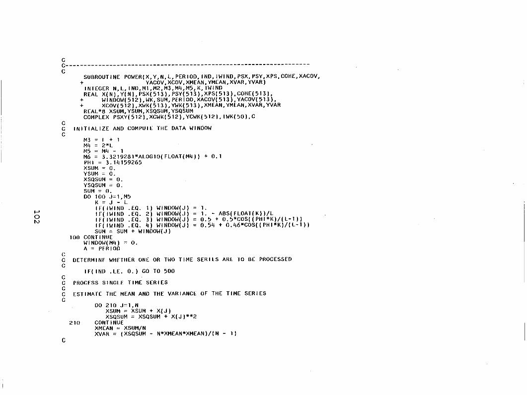
1-' 0 N

c c-------------------------------------------------------------------c

SUBROUTINE POWER(X,Y,N,L,PERIOD, IND, IWIND,PSX,PSY,XPS,COHE,XACOV, + YACOV,XCOV,XMEAN,YMEAN,XVAR,YVAR)

INTEGER N,L, IND,Ml,M2,M3,M4,M5,K, IWIND REAL X(N),Y(N),PSX(513),PSY(513),XPS(513),COHE(513),

+ WINDOW(512),WK,SUM,PERIOD,XACOV(513),YACOV(513), + XCOV(512),XWK(513),YWK(513),XMEAN,YMEAN,XVAR,YVAR

REAL*8 XSUM,YSUM,XSQSUM,YSQSUM COMPLEX PSXY(512),XCWK(512),YCWK(512), IWK(50),C

c C INITIALIZE AND COMPUTE THE DATA WINDOW c

100

c

M3 = L + 1 M4 = 2*L M5 = M4 - 1 M6 = 3.3219281*ALOG10(FLOAT(M4)) PHI = 3.111159265 XSUM = O. YSUM = O. XSQSUM = O. YSQSUM = O. SUM = O. DO 100 J= 1, M5

K = J - L IF(IWIND .EQ. 1) WINDOW(J) IF( IWIND .EQ. 2) WINDOW(J) IF(IWIND .EQ. 3) WINDOW(J) IF( IWIND .EQ. 4) WINDOW(J) SUM = SUM + WINDOW(J)

CONTINUE Wl NDOW( Mit) = O. A = PERIOD

+ o. 1

1. 1. - ABS(FLOAT(K))/L 0.5 + 0.5*COS((PHI*K)/(L-1)) 0.54 + 0.46*COS((PHI*K)/(L-1))

C DETERMINE WHETHER ONE OR TWO TIME SERIES ARE TO BE PROCESSED c

IF( IND .LE. 0.) GO TO 500 c C PROCESS SINGLE liME SERIES c C ESTIMATE THE MEAN AND THE VARIANCE OF THE TIME SERIES c

DO 210 J=1,N XSUM = XSUM + X(J) XSQSUM = XSQSUM + X(J)**2

210 CONTINUE XMEAN = XSUM/N XVAR = (XSQSUM- N*XMEAN*XMEAN)/(N- 1)

c

C CENTER THE TIME SERIES BY SUBTRACTING THE MEAN c

DO 220 J=l,N X(J) = X(J) - XMEAN

220 CONTINUE c C ESTIMATE THE AUTOCOVARIANCE c

CALL COVAR(X,X,N,L,XACOV) c C ESTIMATE THE POWER SPECTRUM c

1-' c

DO 300 J=L, M5 K=J-L+1 XCWK(J) = CMPLX(WINDOW(J)*XACOV(K),O.) XCWK(M4-J) = XCWK(J)

300 CONTINUE XCWK(M4) = (0.,0.) CALL FFT2C(XCWK,M6, IWK)

DO 310 J=1,M3 K = M3+J SHIFT = -2*(K-1)*PHI*(L-1)/(2*L) XCWK(J) = CMPLX(COS(SHIFT),SIN(SHIFT))*XCWK(J) PSX(J) = A*REAL(XCWK(J))

310 CONTINUE RETURN

500 CONTINUE

0 C PROCESS TWO TIME SERIES w c

C ESTIMATE THE MEANS AND THE VARIANCES OF THE TIME SERIES c

DO 610 J=1,N XSUM = XSUM + X(J) YSUM = YSUM + Y(J) XSQSUM = XSQSUM + X(J)**2 YSQSUM = YSQSUM + Y(J)**2

610 CONT 1 NUE XMEAN = XSUM/N XVAR = (XSQSUM- N*XMEAN*XMEAN)/(N- 1) YMEAN = YSUM/N YVAR = (YSQSUM- N*YMEAN*YMEAN)/(N- 1)

c C CENTER THE TIME SERIES BY SUBTRACTING THE MEAN c

c

DO 620 J=l,N X(J) = X(J) - XMEAN Y(J) = Y(J) - YMEAN

620 CONTINUE

1-' 0 >{::>

C COMPUTE THE AUTO AND THE CROSS-COVARIANCES c

c

CALL COVAR(X,X,N,L,XACOV) CALL COVAR(Y,Y,N,L,YACOV) CALL COVAR(X,Y,N,L,XPS) DO 650 J=l,M3

K = L + J XCOV(K) = XPS(J)

650 CONTINUE CALL COVAR(Y,X,N,L,XPS) DO 700 J=l,M3

K = M3 + 1 - J XCOV(K) = XPS(J)

700 CONTINUE

C ESTIMATE THE POWER AND THE CROSS-SPECTRUM c

DO 800 J=L,M5 K=J-L+l XCWK(J) = CMPLX(WINDOW(J)*XACOV(K),O.) XCWK(M4-J) = XCWK(J) YCWK(J) = CMPLX(WINDOW(J)*YACOV(K),O.) YCWK(M4-J) = YCWK(J)

800 CONTINUE XCWK(M4) = (0.,0.) YCWK(M4) = (0.,0.) DO 850 J=1,M4

K = J + 1 PSXY(J) = CMPLX(WINDOW(J)*XCOV(K),O.)

850 CONTINUE CALL FFT2C(XCWK,M6, IWK) CALL FFT2C(YCWK,M6, IWK) CALL FFT2C(PSXY,M6, IWK) COHE(1) = 1. DO 890 J=1,M3

K = M3 + J SHIFT = -2*(K-l)*PHI*(L-1)/(2*L) C = CMPLX(COS(SHIFT),SIN(SHIFT)) XCWK(J) = C*XCWK(J) YCWK(J) = C*YCWK(J) PSXY(J) = C*PSXY(J) PSX(J) = A*REAL(XCWK(J)) PSY(J) = A*REAL(YCWK(J)) XPS(J) = A*REAL(PSXY(J)) XPS(K) = ATAN2(AIMAG(PSXY(J)),REAL(PSXY(J)))/(2*PHI)+0.5 IF(J .EQ. 1) GO TO 890 COHE(J) = XPS(J)*XPS(J)/(PSX(J)*PSY(J)+1E-5)

890 CONTINUE RETURN

END

l-' 0 l/1

c

SUBROUTINE COVAR(X,Y,N,L,COV) INTEGER L,M1,M2,M3,M4,M5,N,J,K REAL COV(1024),V,W,X(N),Y(N) COMPLEX Z(1024),ZX,ZY, IWK(12) COMPLEX*16 ZZ(1024)

C INITIALIZE c

c

M3 = L + 1 M4 = 2*L V= FLOAT(M4) M5 = 3.3219281*ALOG10(V) + 0.1 DO 50 J=1,M4

zz ( J ) = ( 0 •• 0 • ) 50 CONTINUE

C LOOP TO ACCUMULATE RAW POWER SPECTRA c

c

N1 = N - L DO 1000 1=1,N1,L

DO 100 J=l,L K=I+J-1 Z(J) = CMPLX(X(K),-1*Y(K))

100 CONTINUE DO 400 J=M3,M4

K=I+J-1 Z(J) = CMPLX(0.,-1*Y(K))

400 CONTINUE 500 GALL FFT2C(Z,M5, IWK)

C DO EVEN-ODD SEPARATION AND ACCUMULATE CONJG(X)*Y c

ZZ(1) = CMPLX(-0.5*AIMAG(Z(1)*Z(1)). O.)+ ZZ(1) DO 600 J=2,M4

K = J - 1 K1 = M4 + 1 - K ZZ(J) = 0.25*CMPLX(-2*AIMAG(Z(J)*Z(K1)), CABS(Z(J))*

+ CABS(Z(J))-CABS(Z(K1))*CABS(Z(K1))) + ZZ(J) 600 CONTINUE

1000 CONTINUE c C INVERSE DFT TO GIVE COVARIANCE c

DO 1300 J=1,Mlt Z(J) = DCONJG(ZZ(J))

1300 CONTINUE GALL FFT2C(Z,M5, IWK) DO 1150 J= 1 , M4

Z(J) = Z(J)/M4 1150 CONTINUE

z .......

-, N

....J <

<""'W :E:O::

.-Il Il -,--,w o-~ o>zz .-o-c:: .-ul-~

Zl-0 0 owz 0 UO::L.J

0 0 ... ....

106

..... 0 --.]

c-----------------------------------------------------------------------c c c

SUBPROGRAM TO PLOT IN LOG-LOG SCALE

c-----------------------------------------------------------------------c c c c c c c c c c c c c c c c c c c c c c c c c c c

INPUT ARGUMENTS

N - NUMBER OF DATA POINTS TO BE PLOTED X( 1) -X-COORDINAT[ OF 1-TH DATA Y( 1) - Y-COORDINAT[ Of 1-TH DATA Y1( 1) - Y-COORDINATE OF 1-TH DATA OF TitE SECOND SET XORGIN - X-COORDINATE OF THE ORGIN YORGIN - Y-COORDINAT[ OF THE ORGIN OPTION - 1 - AUTOCORRELATION

2 - POWER SPECTRUM IN WAVE NUMBER DOMAIN 3 - POWER SPECTRUM IN FREQUENCY DOMAIN 4 - CROSS-CORRELATION 5 - CROSS-SPECTRUM IN WAVE NUMBER DOMAIN 6 - CROSS-SPECTRUM IN FREQUENCY DOMAIN 7 - COHERENCE SPECTRUM IN WAVE NUMBER DOMAIN 8 - COHERENCE SPECTRUM IN FREQUENCY DOMAIN

VARIABLES USED

XEXMIN - THE MINIMUM X-COORDINAT[ THE THE DATA DXEX - SCALE FACTOR FOR THE X-COORDINAT[ YEXMIN - THE MINIMUM Y-COORDINAT[ Of THE DATA DYEX - SCALE FACTOR FOR THE Y-COORDINAT[ YEXMI1 -THE MINIMUM Y-COORDINAT[ THE THE SECOND SET Of DATA DYEX1 - SCALE FACTOR FOR THE Y-COORDINATE Of THE SECOND SET

c-----------------------------------------------------------------------suBROUTINE LPLOT(N,X,Y,Y1,XORGIN,YORGIN,OPTION) INTEGER N,OPTION REAL X(N),Y(N),Y1(N),XORGIN,YORGIN,XEXMIN,DXEX,YEXMIN,DYEX,

+ YEXMI1,DYEX1,XMIN,XFACT,YMIN,YFACT c C DELETE THE FIRST SET OF THE DATA c

c

lf(OPTION .EQ. 1 .OR. OPTION .EQ. 4) GO TO 53 N = N - 1 DO 50 1=1, N

X( 1 ) = X( 1 +1) Y( 1 ) = Y( 1 +1) Y1 ( 1 ) = Y1 ( 1 + 1 )

50 CONTINUE 53 CONTINUE

C FIND THE MINIMUM VALUE AND SCALE FACTOR FOR A 5 INCH X AXIS AND Y AXIS

1-' 0 ro

c

c c c

c c c

GO TO (51,52,52,51,52,52,52,52), OPTION 51 CALL PSCALE(5.,1.,XMIN,XFACT,X,N,1)

CALL PSCALE(5.,1.,YMIN,YFACT,Y,N,1) CALL PLTOFS(XMIN,XFACT,YMIN,YFACT,XORGIN,YORGIN) CALL PLTREC CALL PLINE(X,Y,N,1,0,0,1) GO TO 55

52 CALL PLGSCL(5.,XEXMIN,DXEX,X,N,1) CALL PLGSCL(5.,YEXMIN,DYEX,Y,N,1) CALL PLTOFS(XEXMIN,DXEX,YEXMIN,DYEX,XORGIN,YORGIN) CALL PLTLOG(3) CALL PLINE(X,Y,N,l,O,O, 1) lf(OPTION .NE. 5 .AND. OPTION .NE. 6) GO TO 55

CALL PSCALE(5.,1. 1YEXMI1,DYEX1,Y1,N,1) CALL PENCHG('RED ) CALL PLTOFS(XEXMIN,DXEX,YEXM11,DYEX1,XORGIN,YORGIN) CALL PLTLOG(2) CALL PLINE(X,Y1,N,1,0,0,1) CALL PLTREC CALL PAXIS(XORGIN-1.,YORGIN,'PHASE OF CROSS-SPECTRUM',

+ 23,5.,90.,YEXMI1,DYEX1,1.) CALL PENCHG('BLAC')

55 CONTINUE

DRAW X-AXES

IFIOPTI?N .EQ. 1 .OR. OPTION .EQ. 4) CALL PAXIS(XORGIN,YORGIN, + r(S) ,-4,5.,0.,XMIN,XFACT,1.)

lf(OPTION .EQ. 2 .OR. OPTION .EQ. 5 .OR. OPTION .EQ. 7) CALL + PLGAXS(XORGIN,YORGIN, 1 WAVE-NUMBER 1 ,-11,5.,0.,XEXMIN,DXEX)

IF(OPTION .EQ. 3 .OR. OPTION .EQ. 6 .OR. OPTION .EQ. 8) CALL + PLGAXS(XORGIN,YORGIN, 1 FREQUENCY(1/S)',-14,5.,0.,XEXMIN,DXEX)

DRAW Y-AXES

lf(OPTION .EQ. 1) CALL PAXIS(XORGIN,YORGIN,'AUTOCORRELATION', + 15,5.,90.,YMIN,YFACT, 1.)

IF(OPTION .EQ. 4) CALL PAXIS(XORGIN,YORGIN, 'CROSSCORRELATION', + 16,5.,90.,YMIN,YFACT,l.)

lf!OPTION .EQ. 2 .OR. OPTION .EQ. 3) CALL PLGAXS(XORGIN,YORGIN +, POWER SPECTRUM 1 ,14,5.,90.,YEXMIN,DYEX)

lf!OPTION .EQ. 5 iOR. OPTION .EQ. 6) CALL PLGAXS(XORGIN,YORGIN +, CROSS-SPECTRUM ,14,5.,90.,YEXMIN,DYEX)

IFIOPTION .EQ. 7 .OR. OPTION .EQ. 8) CALL PLGAXS(XORGIN,YORGIN + , COHERENCE',9,5.,90.,YEXMIN,DYEX)

c C READJUST THE X-ORGIN AND THE Y-ORGIN FOR THE NEXT PLOT c

IF (YORGIN .GT. 15) GO TO 1200

1--' 0 ID

YORGIN = YORGIN + 11. GO TO 1400

1200 CONTINUE YORGIN = 3.25 XORGIN = XORGIN + 9.

1400 CONTINUE RETURN END

1-' 1-' 0

c-----------------------------------------------------------------------c c c c c c c c

PROGRAM:TVOID3

THIS PROGRAM TESTS THE SUBROUTINE VOID3. SINGE ONLY SINGLE CHANNEL DATA IS AVAILABLE AT THIS MOMENT, DUPLICATES OF THE AVAILABLE DATA ARE USED FOR TUE OTUER TWO CUANNEL. ALSO, THE CALI BRAT 1 ON MATR 1 X IS CHOSEN SUCH THAl EACH PROBE IS SENSITIVE TO ONLY ONE DIRECTION.

c-----------------------------------------------------------------------REAL A(3,3),GSCALE(3),GZER0(3),ECRIT1(3),ECRIT2(3),

+ LEVEL1(3),LEVEL2(3) INTEGER DELAY,OPTION,GATE(5000) DO 100 1 =1, 3

DO 200 J=1,3 A(I,J) =O.

200 CONTINUE 100 CONTINUE

DO 300 1=1,3 A( 1 , 1 ) = 84. 4095 GSCALE( 1) = 9.768E-4 GZERO( 1) = O. ECRIT1( 1) = 0.025 ECRIT2( 1) = 0.02 LEVELl(l) = 0.9 LEVEL2( 1) = 0.85

300 CONTINUE NORCRD = 5 LEAD = 30 DELAY = 30 OPTION = 0 GALL VOID3(NORCRD,GSCALE,GZERO,A,ECRIT1,ECRIT2,LEVEL1,

+ LEVEL2,LEAD,DELAY,OPTION,GATE) 500 CONTINUE

STOP END

1-' 1-' 1-'

c-----------------------------------------------------------------------c c c c c c c c c c c

PROGRAM: TPOWERSIN

THIS PROGRAM TESTS THE SUBROUTINE POWER. SERIES

AND X= SIN(T) + 1 Y= 2*COS(T) + 2

IT GENERAlES TWO liME

AT THE SAMPLING RATE OF 5 PER UNIT liME. EACH liME SERIES CONTAINS 5120 SAMPLES. THIS IS DIVIDED INTO 20 EQUAL LENGTH ENSEMBLES FOR liME SERIES ANALYSIS.

c-------------------------------------~---------------------------------c REAL X(5120),Y(5120),F(129),D1(256),D2(512),W1(129),W2(129),

+ W12(129),PHI,C1,C2,C12,T,PSX(258),WPSX(258),PSY(258),WPSY(129) + ,XPS(258),WXPS(129),PHASE(129),COHE(258),XACOV(512),YACOV(512) + ,XCOV(512),XMEAN,YMEAN,XVAR,YVAR,SUM,AREA

c C GENERAlE THE liME SERIES c

c

N = 5120 DO 100 1=1, N

T = 0.2*1 X(l) = SIN(T) + 1. Y( 1) = 2*COS(T) + 2.

100 CONTINUE

C PREPARE INPUT ARGUMENTS AND GALL THE SUBROUTINE POWER c

c

L = 128 M3 = L + 1 M4 = 2*L M5 = M4 - 1 PERIOD = 0.2 IND = 0 IWIND = 3 CALL POWER(X,Y,N,L,PERIOD, IND, IWIND,PSX,PSY,XPS,COHE,XACOV,YACOV,

+ XCOV,XMEAN,YMEAN,XVAR,YVAR)

C USE TRAPEZOIDAL RULE TO ESTIMATE THE AREA UNDER THE POWER SPECTRUM c

c

SUM = PSX( 1 )/2. DO 200 1=2,L

SUM = SUM + PSX( 1) 200 CONTINUE

SUM = SUM + PSX(M3)/2. AREA = 2*SUM/(M4*PERIOO)

C PREPARE HIE SERIES FOR FREQUENCIES, liME OISPLACEMENTS, AND WAVE NUMBERS

1--' 1--' N

c

c

PH 1 = 3. 14159265 Cl = 2*PHI/XMEAN C2 = 2*PHI/YMEAN C12 = 2*PHI/SQRT(XMEAN*XMEAN + YMEAN*YMEAN) DO 300 l=l,M3

Dl(l) = (1- l.)*PERIOD f( 1) = ( 1 - 1. )/(M4*PERIOD) Wl(l) = Cl*f(l) W2( 1) = C2*f( 1) W12( 1) = Cl2*f( 1) WPSX( 1) = PSX( 1)/Cl WPSY( 1) = PSY( I)/C2 WXPS( 1) = XPS( 1 )/C12 PliASE( 1 ) = XPS( M3 + 1 )

300 CONTINUE M2 = M4 + 1 DO 500 l=l,M2

D2( 1) = ( 1 - M3)*PERIOD 500 CONTINUE

C PRINT OUT THE RESULTS c

c

510

520

530

540

550

WRITE(6,5101 XMEAN FORMAT( '0', 1XMEAN = 1 ,f8.5) WRITE(6,520) XVAR fORMAT(lX,'XVAR = 1 ,f8.5) WRITE(6,530) YMEAN fORMAT(lX,'YMEAN = ',f8.5) WRITE(6,540) YVAR fORMAT( lX, 'YVAR = ',f8.5) WRITE(6,550) AREA fORMAT(lX,'AREA UNDER THE POWER SPECTRUM IS ',f8.5)

C PLOT THE RESULTS c C XORGIN = 2. C YORGIN = 3.25 C CALL LPLOT(M3,Dl,XACOV,PIIASE,XORGIN,YORGIN,l) C CALL LPLOT(M3,Dl,YACOV,PiiASE,XORGIN,YORGIN,l) C CALL LPLOT(M2,D2,XCOV,PHASE,XORGIN,YORGIN,4) C CALL LPLOT(M3,f,PSX,PHASE,XORGIN,YORGIN,3) C CALL LPLOT(M3,f,COI-IE,PHASE,XORGIN,YORGIN,8) C CALL LPLOT(M3,f,XPS,PHASE,XORGIN,YORGIN,6) C CALL PLTEND

STOP END

......

...... w

c-------------------------------------------------------------------c c c c c c c

PROGRAM:TESTPOWER1PH

TIIIS PROGRAM DEMONSTRATES USE Of SUBROUTINE 'POWER' TO COMPUTE AND PLOT THE POWER SPECTRUM AND THE AUTOCORRELATION FUNCTION Of TURBULENT VELOCITY FROM SINGLE-PHASE DATA.

c-------------------------------------------------------------------c INTEGER*2 G(1024) REAL GSCALE,GZERO,A,B,C,

+ V(25600),PERIOD,PSX(257),XACOV(257), + f(257),T(257)

NRCRD = 100 N = 25600 L = 256 PERIOD = 0.0004 M3 = L + 1 M4 = 2*L GSCALE = 9.768E-4 GZERO = 0 A= 35.76 B = 6.42 c = 1.53846 1< = 1 DO 200 1=1,NRCRD

READ(5,100)(G(J),J=1,1024) 100 FORMAT(128(8A2))

DO 1000 J=1, 1024,4 G(J) = G(J)/16 E = 1.1136*(G(J)+0.5)*2.442E-4+11.14323 V(K) = ((E*E-A)/B)**C 1< = 1<+1

1000 CONTINUE 200 CONTINUE

CALL POWER(V,V,N,L,PERIOD,1,3,PSX,PSY,XPS,COHE,XACOV,YACOV, + XCOV,XMEAN,YMEAN,XVAR,YVAR)

DO 3000 1=1,M3 WRITE(6,250) PSX( 1)

250 FORMAT(1X,E14.6) f( 1) = ( 1-1 )/(M4*PERIOD) T( 1) = ( 1-1 )*PERIOD

3000 CONTINUE XORGIN = 2. YORGIN = 3.25 CALL LPLOT(M3,T,XACOV,PHASE,XORGIN,YORGIN,1) CALL LPLOT(M3,f,PSX,PHASE,XORGIN,YORGIN,3) CALL PLTEND STOP

0 z w

114

c-----------------------------------------------------------------------c C PROGRAM: TPOWER2PH c C THIS PROGRAM DEMONSTRATES USE OF SUBROUTINES "VOIDl" AND "POWER" C TO COMPUTE AND PLOT THE POWER SPECTRUM Of LIQUID PHASE TURBULENCE C STRUCTURE FROM 2-PHASE fLOW DATA. Il ALSO PLOTS THE POWER SPECTRUM C Of TllE PHASE INDICATOR FUNCTION TO SHOW THE EFFECT OF SEGMENTED C LIQUID PHASE DATA DUE TO THE PRESENCE OF VOIDS. c c-----------------------------------------------------------------------

INTEGER*2 G(1024),LEN INTEGER GATE(5120),DELAY,OPTION REAL GSCALE,GZERO,A,B,C,ECRIT1,ECRIT2,LEVEL1,

+ LEVEL2,V(25600),W(25600),PERIOD,PSX(257), + PSY(257),F(257),XPS(513),COHE(257),XACOV(257), + YACOV(257),XCOV(513)

REAL*8 SUM NRCRD = 100 N = 25600 L = 256 PERIOD = 0.0004 M3 = L + 1 Mil = 2*L M5 = PERIOD*lOOOO + 0.1 GSCALE = 9.768E-4

~ GZERO = O. ~ A = O. 357 ~ B = 0.0627

c = 1.52 ECRITl = 0.025 ECRIT2 = 0.02 LEVELl = 0.9 LEVEL2 = 0.85 LEAD = 30 DELAY = 30 OPTION =0 GALL VOID1(NRCRD,GSCALE,GZERO,A,B,C,ECRIT1,ECRIT2,LEVEL1,

+ LEVEL2,LEAD,DELAY,OPTION,GATE) LEN = 7 CALL CNTRL( 'BSR 100 1 ,LEN,5) SUM = O. NSUM = 0 J = 1 NI = 0 DO 2000 IRCRD=l,NRCRD

READ(5,85)(G( 1), 1=1, 1024) 85 FORMAT(128(8A2))

DO 1000 1=1, 1024,M5 NI = NI + 1

1-' 1-' Q)

90

100 1000 2000

K = ( IRCRD-1)*1024 + 1 lf(K .GE. IABS(GATE(J+1))) J = J + 1 lf(GATE(J) .LT. 0) GOTO 90

G( 1) = G( 1 )/16 V(NI) = (((GSCALE*(G( 1)+0.5-GZER0))**2-A)/B)**C W( N 1) = 1. SUM = SUM + V(NI) NSUM = NSUM + 1 GO TO 100

CONTINUE V( N 1) = O. W( N 1) = O.

CONTINUE CONTINUE

CONTINUE SUM = SUM/NSUM

DO 3000 1=1,N

3000 c

lf(V(I) .GT. lE-3) V(I)=V(I)-SUM CONTINUE

C PRINT THE RESULTS c

c

WRITE(7,50) SUM VMEAN = 1. - fLOAT(M5)*NSUM/(1024*NRCRD)

50 fORMAT(1X,'MEAN LIQUID PHASE VELOCITY IS ',E14.5) WRITE(7,601 VMEAN

60 f0RMAT(1X, VOID fRACTION IS 1 ,E14.5)

C GET THE POWER SPECTRUM c

c

IND = 0 IWIND = 3 CALL POWER(V,W,N,L,PERIOD,IND, IWIND,PSX,PSY,XPS,COHE,XACOV,

+ YACOV,XCOV,XMEAN,YMEAN,XVAR,YVAR)

C PREPARE THE SERIES fOR fREQUENCIES c

DO 3500 l=l,M3 f(l) = (1- 1.)/(M4*PERIOD)

3500 CONTINUE c C PLOT THE RESULT c

XORGIN = 2. YOHGIN = 3.25 CALL LPLOT(M3,f,PSX,PHASE,XORGIN,YORGIN,3) CALL LPLOT(M3,f,PSY,PHASE,XORGIN,YORGIN,3) CALL PLTEND STOP END