FASTER - International Nuclear Information System (INIS)
109
SLAC-482 STUDY OF DEEP INELASTIC SCATTERING OF POLARIZED ELECTRONS OFF POLAIRZED DEUTERONS Masao Kuriki SLAC-Report-482 March 1996 Prepared for the Department of Energy under contract number DE-AC03-76SF00515 FASTER y.-:* v r-i •--
-
Upload
khangminh22 -
Category
Documents
-
view
2 -
download
0
Transcript of FASTER - International Nuclear Information System (INIS)

SLAC-482
STUDY OF DEEP INELASTIC SCATTERING OF POLARIZED ELECTRONS OFF POLAIRZED DEUTERONS
Masao Kuriki
SLAC-Report-482
March 1996
Prepared for the Department of Energy under contract number DE-AC03-76SF00515
FASTER y.-:*vr-i •--

This document and the material and data contained therein, was developed under sponsorship of the United States Government. Neither the United States nor the Department of Energy, nor the Leland Stanford Junior University, nor their employees, nor their respective contractors, subcontractors, or their employees, makes any warranty, express or implied, or assumes any liability or responsibility for accuracy, completeness or usefulness of any information, apparatus, product or process disclosed, or represents that its use will not infringe privately-owned rights. Mention of any product, its manufacturer, or suppliers shall not, nor is it intended to, imply approval, disapproval, or fitness for any particular use. A royalty-free, nonexclusive right to use and disseminate same for any purpose whatsoever, is expressly reserved to the United States and the University.
2/80

SLAC-482 UC-414
Acknowledgments
STUDY OF DEEP INELASTIC SCATTERING OF POLARIZED ELECTRONS OFF POLARIZED
DEUTERONS
Masao Kuriki
Stanford Linear Accelerator Center Stanford University, Stanford, CA 94309
SLAC-REPORT-482 March 1996
This study has been done as a collaborative work of over eighty physicists and graduate students at Stanford Linear Accelerator Center. First, I would like to thank all of the member of the collaboration and the staff of the SLAC for their excellent work.
I appreciate Professor Charles Prescott for all of his support during my staying at SLAC. Special thanks to Professor Charlie Young for his good advice and huge contribution to the analysis. The discussion with Professor Peter Bosted about the error analysis was very fruitful. I am grateful to Dr. Takashi Akagi for his help to everything what I did. Without his critical advice, this thesis would have been impossible. It was a wonderful experience for me working with the graduate students: Todd Averett, Johannes Bauer, Robin Erbacher, Jeff Fellbaum, Philippe Grenier, Tingjun Liu, Paul Raines, and Philippe Steiner. I am especially grateful to Johannes Bauer for his co-work on the operation and the analysis of the Hodoscope system, Robin Erbacher and Paul Raines for their contributions checking my english in this thesis.
I would like to express my deepest thanks to the staff of Tohoku University, especially Proffesor Haruo Yuta giving me the wonderful chance to participate this experimet. The ciritical discussion with Proffesor Koya Abe was very helpful and inspired me.
This thesis was made possible by the supporting and confidence of my family. I appreciate my father and mother for their encouragement both physically and spiritually.
Tin's thesis is dedicated to my best friend, Akihiro Ohaogi died in 1995
Prepared for the Department of Energy under contract number DE-AC03-76SF00515
Printed in the United States of America. Available from the National Technical Information Service, U.S. Department of Commerce, 5285 Port Royal, Springfield, Virginia 22161
'Ph.D. thesis MASTER i t
DISTORTION OF IMS DOCUMENT « OUOID #

Abstract
This thesis describes a 29GeV electron - nucleon scattering experiment carried out at Stanford Linear Accelerator Center (SLAC). Highly polarized electrons are scattered off a polarized ND3 target. Scattered electrons are detected by two spectrometers located in End Station A (ESA) at angles of 4.5° and 7° with respect to the beam axis.
We have measured the spin structure function <h of deuteron over the range of 0.029 < x < 0.8 and 1.0 < Q1 < 12.0 (GeV/c)2 giving the integral of g\ over the range 0 < x < 1 to be 0.0396 ± 0.0035 ± 0.0039 at average Q 2 = 3.0(GeV/c)2.
This integral indicates a discrepancy of more than three standard deviations from the prediction of the Ellis-Jaffe sum rule, J? gfdx = 0.068 ± 0.005 at Q 2 = 3.0(GeV/c)2
while our result of gf in good agreement with SMC results. Combined with g\ of the proton, the measurement of the integral of ${$ - gfjdx = 0.1586±0.0103±0.0162, was consistent with the prediction by the Bjorken sum rule, J^gf - g")dx = 0.169 ± 0.008. We also obtained the strong coupling constant at Q2 = 3.0(GeV/c)2 to be 0.417io;Jfo, using the power correction for the sum rule up to third order of a,. This result is in agreement with the strong coupling constant at(Q2 = 3.0(GeV/c)2) obtained from various experiments.
Using our deuteron results and the axial vector couplings of hyperon decays, the total quark polarization along the nucleon spin is found to be 0.286 ± .055, implying that quarks carry only 30% of the nucleon spin. The strange sea quark polarization is also determined to be —0.101 ± .023. These measurements are in agreement with other experiments and provide the world most precise measurement of these quark polarization.
Contents
1 Introduction 12
2 Theory of the deep inelastic scattering 18 2.1 Spin-averaged cross section 20
2.2 Spin-dependent cross section 22 2.3 Cross section asymmetry 24 2.4 Virtual photon cross section 25 2.5 #1 of deuteron 28 2.6 Sum rules 30
2.6.1 Bjorken sum rule 30
2.6.2 Ellis-Jaffe sum rule 33
3 Experimental setup 36 3.1 Polarized electron 36
3.1.1 Unstrained GaAs 38
3.1.2 Strained GaAs 39 3.2 Beam line 42
3.3 M0ller system 46
3.4 Polarized target 50
3.5 Spectrometers 57 3.5.1 Cerenkov counter 61
* 3.5.2 Hodoscope 64
1

2 CONTENTS
3.5.3 Shower counter 72
3.5.4 Trigger counter 78
3.5.5 Trigger electronics 82
3.6 Data acquisition and data handling 86
4 Analysis 90
4.1 Event selection 90
4.1.1 Beam analysis 90
4.1.2 Shower cluster finding 97
4.1.3 Track finding 99
4.1.4 Electron identification 103
4.2 The cross section asymmetry 116
4.2.1 The dead time correction 118
4.2.2 beam polarization 121
4.2.3 Target polarization 122
4.2.4 Dilution factor 124
4.2.5 Nitrogen correction 126
4.2.6 Positron subtraction 127
4.2.7 Radiative correction 131
4.2.8 Results 135
4.2.9 Study for the systematic effects on the asymmetry 137
5 Results 141
5.1 ffi at a common Q2 141
5.2 Deuteron spin structure function 148
5.3 Proton spin structure function 150
5.4 Neutron spin structure function and sf(i) -g"(x) 1° 2
5.5 systematic error 154
5.5.1 Beam polarization 154
CONTENTS 3
5.5.2 Target polarization 156 5.5.3 Dilution factor 157 5.5.4 Radiative correction 157 5.5.5 Total cross section 158 5.5.6 D-state probability 160 5.5.7 Nitrogen correction 160
5.6 Integrals of gi(x) 162 5.6.1 integral in data region 162 5.6.2 Low x extrapolation 163 5.6.3 High x extrapolation 168
5.7 Test of the sum rules 170 5.7.1 Ellis-Jaffe sum rule for deuteron 171 5.7.2 EHis-Jaffe sum rule for neutron 176 5.7.3 Bjorken sum rule 178
5.8 Quark polarization 183
6 Conclusion and a look into the future 185
A The E143 Collaboration 197
B Spin-dependent cross section 199
B.l Lepton tensor 199 B.2 Hadron tensor 200 B.3 Tensor contraction and the cross section 202
C Kauer and Carlitz model 205
D Derivation of nitrogen correction 208

List of Tables
3.1 Cerenkov efficiency from ADC spectra 64
3.2 Hodoscope dimensions on 4.5° spectrometer 66
3.3 Hodoscope dimensions 7° spectrometer 66
3.4 U-hodoscope dimensions 67
3.5 Time resolution of the hodoscopes 71
3.6 E/P for electron track 77
3.7 Data summary 87
4.1 Time resolution for hodoscope in the tracking 100
4.2 Track classification 100
4.3 Tracking efficiency 103
4.4 Efficiency for electron ID and pion contamination of the requirement for
the Cerenkov counters 106
4.5 Efficiency for electron ID and pion contamination of the requirement for
the E/P ratio 108
4.6 Efficiency for electron ID and pion contamination for neural network . . . 114
4.7 Probability matrix for the dead time correction 119
5.1 Ai{x) for both spectrometers 144
5.2 giW/Fiix) 146
5.3 gi(x)fordeuteron 151
5.4 51 integral for the data region 163
4
LIST OF TABLES 5
5.5 The results of the low-x extrapolation of pi 167 5.6 Fitting with gi(x) at high x region 168 5.7 The integral of gi(x) in the region of 0.8 < a; < 1.0 171 5.8 The integral of gu T at 0} = 3.Q(GeV/c)2 172 5.9 The integral of gu T at Q2 = 10.0(GeV/c)2 172

List of Figures
1.1 r ' from EMC 14 1.2 Aerial view of SLAC 16
2.1 Feynman diagram of the e-N scattering 19
2.2 Polarized cross sections 22
2.3 SU(3) baryon octet 33
3.1 Polarized electron source 37
3.2 Energy level of the unstrained GaAs 38
3.3 Layer of the strained GaAs 39
3.4 The lattice structure of the strained GaAs 40
3.5 Energy level of the strained GaAs 41
3.6 Electron polarization as a function of the photon wave-length 42
3.7 Beam acceleration and transportation 44
3.8 ESA beam line 44
3.9 Beam rastering 45
3.10 Foil array output 45
3.11 Chicane magnets 46
3.12 M0ller polarimeter schematic view 48
3.13 M0ller spectrum 49
3.14 Momentum spectrum of electrons from the M0ller scattering 49
3.15 Energy level for e-P system 52
6
LIST OF FIGURES 7
3.16 Schematic view of E143 polarized target 55 3.17 NMR signal of thermal equilibrium 56 3.18 Schematic view of the spectrometer system 57 3.19 Momentum acceptance of 4.5° spectrometer 58
3.20 Momentum acceptance of 7° spectrometer 58 3.21 Ray trace of in the 4.5° spectrometer 59
3.22 Ray trace of in the 7° spectrometer 59 3.23 Momentum resolution 60 3.24 Cerenkov counter schematic view 62 3.25 Finger overlap 65 3.26 Hodoscope system layout 65 3.27 High voltage splitter 68 3.28 Hodoscope timing sp4 69 3.29 Hodoscope timing sp7 70 3.30 Plane inefficiency for run 1334 in 4.5° spectrometer 73 3.31 Plane inefficiency for run 1334 in 7° spectrometer 73 3.32 The schematic view of the shower counter 74 3.33 Read out of the shower counter 74 3.34 Classification for the shower block (cluster) 76
3.35 Schematic view of the front trigger counter 78
3.36 Schematic view of the rear trigger counter 79 3.37 Cosmic ray test 80 3.38 Time spectrum of the front trigger counter with respect to the counter A 80 3.39 Time difference between counter A and counter B 81 3.40 Time difference between counter B and the front trigger counter 81 3.41 Time difference between counter A and the rear trigger counter. 82
3.42 Time difference between counter B and the rear trigger counter. 82 3.43 E143 trigger logic 83
3.44 Logic of the main trigger 84

8 LIST OF FIGURES
3.45 Logic of pion-or 85
3.46 Logic of the main-or trigger 86
3.47 DAQ system 88
4.1 Spectrum of the Good spill monitor 91
4.2 Spectrum of Bad spill monitor 93
4.3 Spectrum of Toroid 2 current monitor 93
4.4 Spectrum of the beam spot size 94
4.5 The distance of the beam position from the target center 95
4.6 Logic of PRNG 96
4.7 Evolution of Cellular automata 98
4.8 Track extrapolated position on target 101
4.9 Track extrapolated position at the target 101
4.10 Track-cluster matching (sp4) . . . .• 101
4.11 Track-cluster matching (sp7) 101
4.12 CI ADC spectrum (sp4) 104
4.13 C2 ADC spectrum (sp4) 104
4.14 CI ADC spectrum (sp7) 105
4.15 C2 ADC spectrum (sp7) 105
4.16 E/P ratio on 4.5° spectrometer 107
4.17 E/P ratio on 7° spectrometer 107
4.18 Total energy deposited in the nine blocks 109
4.19 The energy ratio of the central block 109
4.20 Energy deposited in 16 blocks beyond the nine blocks 110
4.21 Number of blocks in a cluster 110
4.22 Illustration for the neural network I l l
4.23 Spectrum of the neural network response (sp4) 113
4.24 Spectrum of the neural network response (sp7) 113
4.25 Data profile onx — Q2 plane 115
LIST OF FIGURES 9
4.26 Data profile on x — Q 2 plane 115 4.27 Dead time correction (sp4) 120 4.28 Dead time correction (sp7) 120 4.29 The left-right asymmetry for the dead time correction (sp4) 120 4.30 The left-right asymmetry for the dead time correction (sp7) 120 4.31 The results of ESA M0ller polarimeter 121 4.32 Target polarization 122
4.33 The beam heating correction 123 4.34 Dilution factor (sp4) 126 4.35 Dilution factor (sp7) 126 4.36 Dilution factor due to the positron contamination for A\\ (sp4) 129 4.37 Dilution factor due to the positron contamination for A\\ (sp7) 129 4.38 [Dilution factor due to the positron contamination for Ax (sp4) 129 4.39 [Dilution factor due to the positron contamination for Ax (sp7) 129 4.40 The asymmetric correction due to the positron contamination for A\\ (sp4) 130 4.41 The asymmetric correction due to the positron contamination for A\\ (sp7) 130
4.42 The asymmetric correction due to the positron contamination for Ax (sp4) 130 4.43 The asymmetric correction due to the positron contamination for Ax (sp7) 130 4.44 Feynman diagrams for the radiative correction 132
4.45 Radiative correction for A\\ (sp4) 133 4.46 Radiative correction for Ax (sp4) 133
4.47 Radiative correction for A\\ (sp7) 134
4.48 Radiative correction for Ax (sp7) 134 4.49 Radiative correction for the statistical error of A\\ (sp4) 135 4.50 Radiative correction for the statistical error of A\\ (sp7) 135
4.51 A\\ (sp4) 136
4.52 Ax (sp4) 136
4.53 A\\ (sp7) 136 4.54 Ax (sp7) 136
10 LIST OF FIGURES
4.55 The x 2 distribution of the difference of the A\\ taken with different target polarization direction in 4.5° spectrometer 137
4.56 The x 2 distribution of the difference of the AA. taken with different target polarization direction in 4.5° spectrometer 137
4.57 The x 2 distribution of the difference of the A\\ taken with different target polarization direction in 7° spectrometer 138
4.58 The x 2 distribution of the difference of the As. taken with different target polarization direction in 7° spectrometer 138
4.59 The x 2 distribution of the difference of the A\\ taken with different magnetic field direction in 4.5° spectrometer 139
4.60 The x 2 distribution of the difference of the A± taken with different magnetic field direction in 4.5° spectrometer 139
4.61 The x 2 distribution of the difference of the A\\ taken with different direction of the magnetic field in 7° spectrometer 140
4.62 The x 2 distribution of the difference of the Ax taken with different direction of the magnetic field in 7° spectrometer 140
5.1 A^x) 142 5.2 The difference between A\ (x) from both spectrometers 142
5.3 Si/Fi 143
5.4 The difference of between gi/Fi from both spectrometers 143
5.5 The gi(x)/Fx(x) for deuteron 147
5.6 A\ (x) for deuteron 147
5.7 F2(x, Q2 = 3.0) by NMC parameterization 148
5.8 R{x,Q2 =3.0) 148
5.9 g{(x) 149
5.10 gi(x) for proton 150
5.11 The neutron gY(x) 153
5.12 §?(x) - S ? ( x ) 153
LIST OF FIGURES 11
5.13 Systematic error of xgf(x) due to the beam polarization 155 5.14 Systematic error of xgf (x) due to the target polarization 155 5.15 The systematic error of xgf{x) due to the dilution factor 158 5.16 The systematic error of xgf (a;) due to the radiative correction 158 5.17 F2(x, Q2) from NMC experiment 161
5.18 Systematic error of xgf(x) due to the F\/D' 161 5.19 F2(x) from NMC and the reduced x 2 of the Regge fit 164 5.20 Low x extrapolation of gi of deuteron 165 5.21 Low x extrapolation of g\ of neutron 166 5.22 Low x extrapolation of g\ — g" , 166 5.23 High x extrapolation of the gi(x) for deuteron 169
5.24 High x extrapolation of the gi for neutron 169 5.25 High x extrapolation of g\{x) -g? {x) 170 5.26 xgx(x) for deuteron at Q2 = 10(GeV/c)2 174 5.27 Td results with the prediction of the Ellis-Jaffe sum rule 175 5.28 gi{x) for neutron at 0} - 2.0(GeV/c)2 176 5.29 Tn results with the prediction of the Ellis-Jaffe sum rule 177 5.30 xgl-xgl at Q 2 = 10(GeV/c)2 179 5.31 T p - T" results with the prediction of the Bjorken sum rule 181 5.32 The strong coupling constant as a function of Q2 182 5.33 Quark polarization 184
6.1 Feynman diagram of Photo-gluon fusion 188
C.l Kauer Carlitz model for i4i(a;) 207
D.l Proton polarization 210 D.2 15iV polarization 210

Chapter 1
Introduction
The electron-nucleon scattering has played an important role in advancing our understanding of the nucleon structure. In Quantum electrodynamics (QED), the electron is treated exactly as a point like particle which does not have any structure, whereas the nucleon is treated as a substance which have a complex structure. In electron-nucleon scattering, virtual photons are exchanged between the electron and the substructure of the nucleon. Therefore, this makes us to investigate the nucleon structure by using the photon probe.
In the 1950's, the elastic and quasi-elastic electron-nucleon scattering experiments[l] indicated that the nucleon has a finite size of order 10"X3cm. Several experiments in the middle of 1960's[2] established that the cross section fell with increasing momentum transfer, suggesting a composite nucleon model. In 1969, results from deep inelastic scattering of electrons off a hydrogen target at SLAC[3] showed that the cross section is larger than expected by the composite model, and that the cross section has only a weak dependence on momentum transfer(Q2). This behavior, refer to Bjorken scaling, is interpreted to imply that the nucleon is composed of point-like charged particles. These point like particles were named as partons by Feynman in 1967. The precise measurement of the nucleon structure[4] showed that the charged partons carry only a half of the nucleon momentum, and that neutral partons which carry the other half of the nucleon momentum
12
13
exist in the nucleon. These charged and neutral partons are later identified as quarks and gluons which are described by Quantum Chromodynamics(QCD). Now, we believe that the nucleon is composed of valence quarks, sea quarks, and gluons. There are three valence quarks in the nucleon which determine net quantum numbers such as charge and baryon number. Sea quarks are created in pair by gluon which have no net quantum number. Gluons mediate the color force which composes these partons together.
As nucleon spin is 1/2, it had been assumed that only the valence quarks are responsible for the nucleon spin analogous to the baryon number or nucleon charge, and that sea quarks and gluons were not polarized in the nucleon. In such a naive picture, the SU(6) model of baryons describes well the magnetic moments of the baryons [5].
Bjorken derived a sum rule for the combination of the structure functions of the proton and neutron using current algebra and an assumption of iso-spin symmetry[6]. This sum rule predicts that the integral of the difference of spin structure functions of the proton and the neutron over Bjorken x from zero to one is equal to a sixth of the axial vector coupling strength in neutron beta decay, JjJ[(fifa) — g?(x)]dx = g&i/sv. Because this sum rule can be derived also using QCD calculations, it is thought of as a fundamental sum rule. Bjorken himself said 'If the sum rule is violated, QCD is wrong.'[7]. This sum rule is usually called the Bjorken sum rule.
Ellis and Jaffe derived another sum rule predicting the spin structure functions of the proton and neutron[8j separately, /J g{M(x)dx = ±^{F+D) + (3F-D) where the sign is plus for proton, minus for neutron and F and D are the hyperon decay constants. They assumed the SU(3) flavor symmetry and unpolarized sea quarks. The sum rule obviously depends on the nucleon model, so that it is thought to be less fundamental than the Bjorken sum rule. This sum rule is referred to the Ellis-Jaffe sum rule.
Even though these sum rules were established in the early 70s, we had to wait for the experimental proof until 1976 when deep inelastic scattering of polarized electrons and polarized nucleons was possible along with the development of polarized electron beam and polarized nucleon. The experiment was carried out by the SLAC-Yale collaboration [9], where a large asymmetry was observed as predicted by the quark-parton model. Their

14 CHAPTER 1. INTRODUCTION
results[10] were consistent with the Ellis-Jaffe sum rule for the spin structure function of proton within their large experimental error.
10-93
0.18
1 0.12 fc-~,
0.06 h
, ELLIS-JAFFE Sum Rule
•EMC •SLAC
Hff|4. 0.02
X 0.1
m 0.5
7542A5
Figure 1.1: The integral of the spin-dependent structure function gi(x) for the proton with EMC and SLAC data. The horizontal axis shows Bjorken x in logarithm scale. The vertical axis is the integral of the g\(x) down to the x value. The arrow on the vertical axis shows the Ellis-Jaffe sum rule for the proton. The smooth extrapolation toward x=0 indicates that the extrapolated value is different from the prediction.
In 1988, EMC(European Muon Collaboration) at CERN published the results from high precision measurements of the scattering of polarized muons off polarized protons in butanol[ll], indicating that the spin structure function of the proton was in disagreement with the Ellis-Jafte sum rule as shown in Figure 1.1. They concluded that the quark carries only a small fraction of the proton spin and the strange sea quark has a significant fraction of opposite polarization with respect to the proton spin. This new and surprising .results were called as 'the spin crisis' and denied the naive idea that only valence quarks carry the nucleon spin, and sea quarks and gluons are not polarized.
The E142 Collaboration at SLAC published the results from the first measurement
15
of the neutron spin structure function using 3He target [12]. Their results were consistent with the Ellis-Jaffe sum rule at Q2 = 2.0(GeV/c)2 within one standard deviation x and with the Bjorken sum rule obtained using the QCD correction to third order in a, within one standard deviation. However, their measurements denoted that the quark carried only about a half of the nucleon spin.
These measurements suggested that our understanding of the nucleon spin is far from the whole picture. We need not only to do more theoretical work, but also more experiments. Where is the other part of the nucleon spin? Why do quarks carry only a small fraction of whole nucleon spin although the SU(6) model is successful for predicting the magnetic moment of baryons. We have to find answers for these questions.
This 'Spin Crisis' has led several experiments to measure the nucleon spin structure functions to find the answer, and to reach further understanding of the nucleon spin; the Spin Muon Collaboration (SMC) at CERN [15],[16], HERMES at DESY[17] and E143 at SLAC (18],[19).
The E143 is an international collaboration consisting of about 90 physicists and graduate students from 17 institutes. The purpose of E143 was to investigate the spin structure functions of both the proton and the deuteron. The experiment was implemented using the highly polarized electron beam accelerated by the Linac and the solid ammonia target located in End Station A (ESA). Figure 1.2 shows the aerial view of the SLAC. The long structure stretched from up to down is the 3 km long Linac. The building at the end of the Linac is ESA. The experiment was carried out in ESA with the high statistics. This high statistical measurement was able to test the Ellis-Jaffe and Bjorken sum rules with a higher accuracy than the EMC and E142 measurements. It gave more understanding of how the nucleon spin is carried by quarks. The variation of the beam energy also provided the information of Q2 dependence of the spin structure functions.
This thesis describes E143 investigating the electron scattering off deuterons in ND3
*A reanalysis by D. M. Hawaii and 3. A. Dunne is giving the integral of the gi for neutron to be
—.035 ± .009 which is two standard deviations away from the prediction by Ellis-Jaffe [13] [14].

16 CHAPTER 1. INTRODUCTION
Figure 1.2: Aerial view of the Stanford Linear Acceleration Center. The long structure stretched from up to down is 3 km long Linear accelerator (Linac). The building at the end of the Linac is End Station A where the experiment was carried out.
17
at 29 GeV and presents the results from this experiment. This measurement determined the spin structure function 51 of deuteron with high accuracy. The covered x range is 0.029 < xBj < 0.8 at an average Q 2 = 3.0(GeV/c)2.
In Chapter 2, the formulae of deep inelastic electron-nucleon scattering are derived. The principle of spin structure function measurement and the Ellis-JafFe and Bjorken sum rules are explained. The experimental setup and devices are described in Chapter 3. In Chapter 4, the analysis procedures to reconstruct electron tracks and to calculate the cross section asymmetry including various corrections will be explained. In Chapter 5, the measured data and the results of the structure function and the integral are given including the estimation of systematic errors. Finally, a conclusion and a look into the future are given in Chapter 6.

Chapter 2
Theory of the deep inelastic scattering
Electron-nucleon scattering at large momentum transfer range occurs mainly through the exchange of a photon in electromagnetic interactions. Figure 2.1 shows the Feynman diagram of electron-nucleon scattering, where k and k' are the four momenta, s and s' are the polarization vectors of the electrons in the initial and final states, 0 is the angle of the scattered electron with respect to the electron direction of the initial state, q is the four momentum transfer defined by q = k — k', p is the four momentum of the nucleon, and A is the polarization vector of the nucleon. The gray circle at the photon nucleon vertex involves complex interactions due to the substructure of the nucleon and hadron-ization process. The substructure of the nucleon is parameterized later using several assumptions. Lines from the circle indicate particles coming out from fragmentation of the initial nucleon.
The momenta of the particles involved in this process are expressed as
*„ = ( £ , $ , (2.1)
P / 1 = (M,5), (2.2)
/£ = (£',&')> (2.3)
where E and k are the energy and the momentum for the electron of the initial state, E' and 0 are the energy and the momentum for the electron of the final state, and M is the
nucleon mass.
18
19
mass,
Figure 2.1: Feynman diagram of electron-nucleon deep inelastic scattering
We also define several kinematical variables for our convenience neglecting electron
Q 2 = - 9
2 = 2(k • k') = 2EE'(l-cos9)
= AEE' sin2(0/2)
= 2MxyE, (2.4)
v = E-E\ (2.5)
X 2p-q 2Mu' ( 2 S )
V E p-k' V-1'
The variable x is called 'Bjorken x' and sometimes denoted as XB-
In the following sections, the cross sections for the unpolarized and polarized processes, ie. the spin-averaged and spin-dependent cross sections for the deep-inelastic e-N scattering will be described. The spin structure function, gx is expressed using the spin-averaged and spin-dependent cross sections. After that, the sum rules giving predictions for the integrated value of g\ will be explained.

20 CHAPTER 2. THEORY OF THE DEEP INELASTIC SCATTERING 2.1. SPIN-AVERAGED CROSS SECTION 21
2.1 Spin-averaged cross section
The spin-averaged cross section is that of electron scattering off nucleons averaged over the electron and nucleon spin of the initial and final states. Using the assumptions as discussed in Appendix B.2, the differential cross section in laboratory system is expressed as given in Equation (B.23) by
cPa E l£m - W ^ ^ [W2M)+2t^mWlM^)}, (2.8) where W\{y,Q2) and W2(u,Q2) are the nucleon structure functions of two independent kinematical variables, v and Q2. If we impose the Bjorken scaling of the structure functions in the limit of (u, Q2 -+ oo), the structure functions can be written as a function of a single variable, x, by
(2.9) *",(*)= lim MW^Q2) V,Q3-HX>
F2(x) = lim vW2{v,Q2) f,Q a->oo
(2.10)
The scaling means that the structure function depends only x which is proportional to the ratio of the Q2 to the v, and is independent of Q2 or v as demonstrated by many experiments. This scaling denotes that the deep inelastic scattering of electron and nucleon is interpreted as the incoherent sum of the elastic scattering of electrons and charged partons (quark) in nucleons and x is interpreted as the momentum fraction which the scattered quark has in the nucleon. This experimental fact is an evidence that the quarks compose the nucleon. Scaling is now explained by the asymptotic freedom in QCD: the strong coupling constant depends on the momentum transfer Q2 and it decreases with increasing momentum transfer. The quark acts like a free particle in the large Q2 region due to the small strong coupling constant.
As mentioned in Chapter 1, a nucleon is composed of three valence quarks, sea quarks, and gluons in the Parton Model picture. Because the gluon does not contribute to the electromagnetic interaction, the structure functions, F\[x) and F2(x) are expressed as the incoherent sum of the quark distribution functions, <fr(t (4-)>a:) and gi(t (-JOi1) for
the quarks and anti-quarks by
Fi(x) = 5l!)e?[«,«(t.a;) + ?.(t»a;)+9<(4.la:)+gi(-J-»a:)] (2.11)
-&(*) = ^T,xe'ih(.tx) + gi(-[^) + qi(i„x)+gi(i.)x)}, (2.12) £ i
where the sum is taken over all quark flavors and the arrow denotes the quark helicity with respect to the nucleon spin. The largest contribution to these functions comes from the light three quarks and those from the heavy flavors, c, b, and t are suppressed due to the heavy masses of c, b, and t quarks.
The spin-averaged cross section is rewritten using these new functions by cPa E r i \[lF2(x) + ^tm2(9/2)F,(x)}. (2.13) dE'dQ. 16n2Q2tm2(6/2)E'
The spin-averaged cross section can be expressed using the Fi(x) and R(x) which is the cross section ratio for the longitudinally and transversely polarized virtual photons. Using the R(x) defined by Equation (2.47), the relation between Fj(x) and ^(a;) is given
by _ 2x(l + R)
where 7 is 2 _ 4M2x2 Q2
Q2 ~ v2 r = -or- = ^ (2.15) Substituting the Equation (2.14) into the Equation (2.13), the unpolarized cross section is expressed using the F\ and R as,
(Po e4 E 4(E + E') Fx(x)
where D' is given by
with
cLE'dQ, 16n*Q2E> vM D'
Dl=(l-j)(2-y)
.1 >
£ =
y(l + eR) '
1 l + 2(l + ^)tan 2 (0/2) '
(2.16)
(2.17)
(2.18)

22 CHAPTER 2. THEORY OF THE DEEP INELASTIC SCATTERING 2.2. SPIN-DEPENDENT CROSS SECTION 23
2.2 Spin-dependent cross section
In the polarized electrons scattering off polarized nucleons, the cross section depends on the helicities of both particles of the initial state. We define the four cross sections of the polarized process for the different directions of the electrons and nucleons in the initial state as shown in Figure 2.2. The nucleon is polarized longitudinally or transversely to the electron beam axis. The electron is polarized along the beam axis, parallel or anti-parallel. The combinations of these two electron and nucleon spin states compose the four cross sections. The two cross sections for the longitudinally polarized nucleon are called as the parallel configurations and those for the transversely polarized nucleon are called as the perpendicular configurations.
a •H a rtt
4
-t
Beam axix
a1* a Paralell Perpendicular
t H
Nucleon Spin
Electron Spin
Figure 2.2: Definitions of the cross sections for the four combinations of the electron and nucleon spin. The gray and black arrows indicate the direction of the spin for nucleons and electrons respectively, where the electron beam direction is from bottom to top. The nucleon is polarized longitudinally or transversely with respect to the beam axis. The electron is polarized parallel or anti-parallel to the beam axis. We call these cross sections as the longitudinal or transverse configurations according to the direction of the nucleon spin. The cross sections are indicated by a with two arrows for superscripts. The two arrows show the spin direction of nucleons and electrons respectively.
To extract the spin dependent part of the cross sections for the parallel and perpen
dicular configuration, we give the following cross section differences of the two different
orientations of the electron spin as derived in Equations (B.24) and (B.26),
^ S i P -16^5 4E'H sin ° l M G i ^ Q 2 > + 2 E G > <*• Q 2 > ] • ( 2 - 2 « where G\ (v, Q2) and G2{u, Q2) are the spin structure functions and H is the sign of the inner product of the nucleon spin vector and the momentum of the scattered electron in the perpendicular configuration.
While Wi(y,Q2) and Wi(u,Q2) represent the spin-averaged structures of nucleons, Gi(u,Q2) and G2(u,Q2) are the spin-dependent structure functions of the nucleon. We expect to see a scaling of the spin structure functions in analogy to the spin-averaged structure functions:
(2.21) 9l(x)= lhn M2uGx(u,Q2),
g»(x)= lim Mv2G2{v,Q% i»,Q 2-»oo
(2.22)
where gi(x) and 02fa) are the spin structure functions in the scaling limit. The cross section differences are expressed in terms of the scaled spin structure functions, 51(0;) and g2(x) by,
d V t t - g t t ) dE'dn
E' Wn2Q2 E~
#(0^-<r<-t) E' AE'Hsm6 gi[x) 2E
~M7 + WS92W
(2.23)
(2.24) dE'dQ 16n2Q2E' Similar to jF\(a;) or Fz^x), the spin structure function 01 is expressed by the quark
distributions as,
9i(x) = ^T,eH<li(t,x) + gi{tx)-qi(i,x)-qi{i,x)] i
(2.25)
where i is the quark flavor and Ag,- is defined to be the helicity distribution of a quark
flavor labeled i, Ag,(a;) = [g,(t,s) + gifts)] - [g,(4-,x) + gi(J.,x)].

24 CHAPTER 2. THEORY OF THE DEEP INELASTIC SCATTERING
On the other hand, the spin structure function 92 has no explicit interpretation in the parton model. It relates the quark momentum transverse to the nucleon momentum. g2 is expected to be small in contrast to the g\ and sensitive to the higher twist effect in QCD[20].
2.3 Cross section asymmetry
In order to investigate the spin structure of nucleons, we measure the asymmetries of the cross sections for the different spin orientation of electrons instead of the cross section difference. Two cross section asymmetries for two different nucleon spin direction, parallel and perpendicular to the electron beam are defined by
at* - fftt 4n =
4 L =
(2.26)
(2.27) dr<-+ + <7<-t' where the notation of the cross sections are the same as given in Figure 2.2. An advantage of using the cross section asymmetry over the cross section difference is that the target density, the spectrometer acceptance and, the detection efficiency are canceled in the asymmetry which reduces the systematic errors due to these factors.
Substituting Equations (2.16), (2.23) and, (2.24) into Equations (2.26) and (2.27), the cross section asymmetries are expressed in terms of the structure functions to be,
. E'Hsin9 D' \ , . IE . ,1 A^WTmm\-9i{x)+~92{x)\-
:*) (2.28)
(2.29)
The spin structure functions g\(x) and g2{x) can be expressed in terms of the cross section asymmetries by
ffi(s) = Fx(x)
52(3) = 2sin0£>'
A\\ + tan | A X
E'cosO + E Ai.-.ffsm0./l||
(2.30)
(2.31)
2.4. VIRTUAL PHOTON CROSS SECTION 25
These formulae show that the spin structure functions for nucleons, gi(x) and g2{x) are derived from the measurements of the cross section asymmetry.
2.4 Virtual photon cross section
For studying the nucleon structure, the virtual photon-nucleon interaction provides more direct information for the spin dependent scattering than the electron-nucleon scattering process.
For the photon-nucleon scattering, only four cross sections are independent under the assumptions of angular momentum conservation, parity and time reversal invariances. These four cross sections are given with the following helicity configurations by,
• fc^s) : U,-i;l,4)
aL : : (0,i;0,i) aTL : ; &-b°>b
where the first two numbers in the parenthesis denote the the helicities for the initial photon and nucleon, and the second two numbers for the final photon and nucleon respectively. These cross sections are expressed in terms of the nucleon structure functions by [21]
4 = M i n F i + S i - — 4 (2-32)
T 47rza r_ 2Mx 1 , . „„.
4-OTr-*+—4 (2-33)
aL 47r 2afl A , J / 2 \ _ 1 _ (2.34)
° = — T ^ - b i + 5 2 ] , (2.35)
where K is the flux of the virtual photons defined by K = v — ^ [ 5 ] . K Mv
lorl \wt T{ — it . 2Afl

26 CHAPTER 2. THEORY OF THE DEEP INELASTIC SCATTERING
Using these cross sections, we introduce the new asymmetries Ai and A2 for the
virtual photon-nucleon scattering as follows,
af-oT M = -^—f, (2.36)
/ t 2 = = ^ + ^ - ( 2 , 3 7 )
This A\ is similar to the J4|| in Equation (2.26), but polarized electrons are replaced by the polarized virtual photon. Using Equations (2.32), (2.33), and (2.35), A\ and Ai can be expressed in terms of the spin structure functions by
^i(aO = ^(Si(s)-7 2<72(s)), (2.38)
A2{x) = ^r(gi(x)+g2(x)). (2.39)
We notice that the factor 7 2 is very small (typically, less than 0.05) in our kinematical region. Therefore, gi(x) dominates the virtual photon asymmetry A\. If the term of the 7 2 52(E) is neglected in Equation (2.38), A\{x) can be expressed in terms of the quark distributions by
A ,Ty 9i(x) _ S{e2[g((t,30 + gi(t,s)-g,(4o3)-gi(4-.3)] / 2 4 m
A m ~ Ft(x) ~ Ei e?[ft(t,*) + «(t,*) + <b{i,*) + m>*)] * K '
where g,- is defined in Equation (2.12). In the naive SU(6) model, the Ai(x) is given to be 5/9 for the proton and 0 for the neutron.
Via the virtual-photon cross section asymmetry A\(x), the cross section asymmetry A\\ can be expressed in terms of the parton distribution. From Equations (2.30), (2.31), (2.38) and (2.39), the cross section asymmetries J4|| and Ax are expressed in terms of the virtual photon cross section asymmetries, Ai and A2 by
Al](x) = D(Al(x)+VA2(x)) (2.41)
Aj_(x) = d(A2(x) - CAl{x)) (2.42)
2.4. VIRTUAL PHOTON CROSS SECTION 27
where D, d, 7], and C are the kinematical quantities defined by[22]
C - 2 ^ . (2-46)
with 6 denned in Equation (2.18) and R{x) is the cross section ratio for longitudinal to transverse virtual photon defined by,
R=^Tl^r- (2-47) o\ + o\
Substituting Equations (2.32), (2.33), and (2.34) into Equation (2.47), the R is expressed in terms of the F\(x) and F2(x) by
-K) MF2
v F l 1- (2-48)
In Equation (2.41), the contribution from the second term in the right-hand side is small due to the small factor, t) (typically 0.1) and the small quantity, A2{x) in contrast to A\{x). Therefore A\\ is nearly proportional to A\ which is expressed in terms of the parton distributions. The D in Equation (2.41) is the proportional coefficient between Ai(x) and A\\(x) and is called as the depolarization factor. It is a pure QED factor indicating the depolarization effect of the process of the emitting the virtual photon. Using the depolarization factor, the i4||(a;) is expressed in terms of the parton distributions by
A„(x\ ~ n£' e?fo(t>*) + ft(t.s) - ftCUs) - ftfoafl] , , 4 < n
W> -^S,e*[»(t,*)+«(t,*) + «tt.*) + fia,»)]* K ' where the depolarization factor decreases with the increasing x as D ~ 0.78 at x — 0.03 and D ~ 0.23 at x = 0.8. Therefore, the investigation for the A\\ is equivalent that for the helicity distribution of the quarks in the nucleon with an analyzing power of the factor
D.

28 CHAPTER 2. THEORY OF THE DEEP INELASTIC SCATTERING
2.5 gi of deuteron
The deuteron is a system consisting of a proton and a neutron. The spin structure function for deuteron, then, can be expressed in terms of those functions for proton and neutron.
The deuteron is a spin 1 and parity even particle composed of two spin 1/2 nucleons. Thus, the deuteron is a mixture of S (L=0) and D (L=2) states. These S and D states are expressed using the Clebsh-Gordon coefficients by
\J=l,Jz = l>s = \L = 0,Lz = 0>\S = l,Sz = l> (2.50)
\J=l,Jz = l>D = S\L = 2,Lz = 2>\S=l,Sz = -l> T 1Q\L = 2,Lz = l>\S = l,Sz = 0>
+ v ^ | L = = 2 , L z = = 0 > | 5 = 1 " s , z = 1 > ' ( 2 , 5 1 )
where J and Jz are the magnitude and the Z-component of the total angular momentum,
i(S), Lz(Sz) are the magnitude and the Z-component of the orbital angular momentum
(spin).
A probability that a nucleon spin is anti-parallel to the deuteron spin in the D-state
is calculated to be
i + >4 (2-52)
where 0.5 comes from that one of two nucleons has a spin anti-parallel to the deuteron spin in the Sz — 0 state. If the polarized deuterons contain the D-state with a fraction WD, the deuteron cross section, a^, is expressed in terms of nucleon cross sections, 0$ and <r$ by
<$=(I-±U>D)<TV + IWD*8, (2.53)
where the first arrow is the nucleon spin and the second arrow is the helicity of electron.
The nucleon cross section is the sum of those for the proton and neutron, o> = ap + a„.
2.5. Gi OF DEUTERON 29
Similarly, a^ can be written by,
a j*=( l - | u ,x>)a t f + §«>i>*#, (2.54)
Taking into account the D-state probability, the cross section asymmetry of the deuteron is described as follows
/rti __ /rtt O _ti _ -ft Ad _ ad °d _ it «,„ \aN aN f o e O
A*~w^~{ 2WD)WTO$' ( 2 , 5 5 )
where we assume the parity invariance on the cross sections, ie. a$ = o$, 0$ = 0$ , and a§ = 0$.
Equation (2.55) shows that the asymmetry of the deuteron is smaller than the spin-aligned proton and neutron system by a factor of (1 - -wp). The Aj for deuteron is expressed in terms of the A^'" for proton and neutron with conventions of c^ = 2F$, <rP = F?,an = F?1 by
4-&-§«»> ( 4 $ + ^ ) . ( 2 - 5 6 ) Similarly, the transverse asymmetry, A±, is expressed by
^ = ( l -^ ) (^ + ^g) ( (2.57) Using these equations, the spin structure function gd for deuteron is expressed in terms of those for proton and neutron, g\ and 5" by
2 t f = ( l - f t i > D ) ( r f + t f ) . (2.58)
Under the assumption that the D-state probability WD is independent of x, we can integrate Equation (2.58) and obtain the relation between the integrals of deuteron, proton, and neutron,
2rf=(i- | tm,)(rf + r?), (2.59) where r{ is given by
r{= fdxgHx), (2.60) JO
where i stands for deuteron, proton, and neutron denoted by d, p, and n. 'The factor for the Ff giving the cross section is identical for proton, neutron, and deuteron. Then,
the factor is canceled in the formula of the asymmetry.

30 CHAPTER 2. THEORY OF THE DEEP INELASTIC SCATTERING
2.6 Sum rules
The Bjorken and Ellis-Jaffe sum rules will be explained in this section. These sum rules give predictions on integrals of the spin structure function gi(x) over x range from 0 to 1. The confirmation of these sum rules is the most important purpose in this experiment because we can examine the spin structure of the nucleon and the dynamics of the quarks with these sum rules.
2.6.1 Bjorken sum rule
The Bjorken sum rule is originally derived by Bjorken base on current algebra assuming Iso spin symmetry on proton and neutron quark distribution function[6], giving that the integral of the difference of spin structure functions g\ of proton and neutron is equal to one sixth of the neutron beta decay axial coupling. Now, this sum rule is derived by QCD calculation [23] and is also called as the QCD sum rule.
The original derivation of the sum rule is based on current algebra stated from the ratio of the axial vector coupling constant to the vector coupling constant of neutron beta decay which is expressed in terms of the quark distributions by [24]
- { | [«"(t) - «"(+)] - \ [d"(t) - dP(I)]}, (2.61)
where the up(-n) and d?W are the distribution functions of u and d quark including both of quark and anti-quark of proton (neutron) with the Z-component of the spin to the nucleon spin indicated by the arrows. Under the iso-spin symmetry, vP = d" and d? = u", and the ratio is given by
= Au-Ad, (2.62)
where Ag,- is defined to be <$ (t) — 9? (40 which is explained to the expectation value of
the helicity of the quark flavor i in the proton.
2.6. SUM RULES 31
Assuming that u, d, and s quark exist in the nucleon, gi(x) in (2.25) derived from Parton model can be written by
i
= ^Au{x) + ±Ad(x) + ±As(x), (2.63)
where e< is the charge of the quark i in the unit of electron charge. (fi(x) and g?{x) are expressed with the iso-spin symmetry by,
2<rf(x) = i z W M + ±Ad?{x) + iAs't*), (2.64)
2g?(x) = iAu"(s) + iAcP(ar) + J A S " ^ ) , (2.65)
where the quark distribution functions correspond to that in proton. If we subtract g" from g\, we can obtain the difference without the strange quark:
Sfts) - 9tt*) = I lAu(a:) - Ad(x)]. (2.66)
These Au(x) and Ad(x) are the helicity distribution of the u and d quarks with the momentum fraction x. The integral of these helicity distribution over x gives the expectation value of the helicity in the proton to be,
£ f g ^ = A9 (* = M). (2.67)
Therefore, the integral of the Equation (2.66) over x is given to be
ri-T? = i [Au-Ad]. (2.68)
Inserting Equation (2.62) into Equation (2.68), we obtain the Bjorken sum rule;
r?-r? = i^i. (2.69) ogv
The only assumption used to derive the Bjorken sum rule is iso-spin symmetry which is a fundamental principle in particle physics. Therefore, this sum rule was thought to be fundamental. However, we can not compare this prediction with the measured results

32 CHAPTER 2. THEORY OF THE DEEP INELASTIC SCATTERING 2.6. SUM RULES 33
directly because this sum rule is valid only in the scaling limit, ie. Q2 = oo. Although the scaling of the s tructure function is a good approximation, the s tructure function has Q2 dependence as observed as the scaling violation due to the QCD effect. To make precise comparison of measurements with the Bjorken sum rule, the prediction of the Bjorken sum rule has t o be corrected to the value a t an actual kinematical region of the measurements.
The QGD correction is calculated to third order of the strong coupling constant
a,[25] to be
i - T - 8 j B ( ? ) ' - a M 8 ( ? ) T (2-70) />ro-tf(*)]Hr*-r = i^
The predicted value a t Q2 = 3 .0(GeV/c) 2 with a, = 0.360 ± .050[26] 2 and gA/gv = 1.2573 ± 0.0028(26] is,
V - T n = 0.169 ± .008, (2.71)
where the error was estimated from the ambiguities of the strong coupling constant and the neutron axial vector coupling.
From Equation (2.70), the ratio of the Tp — Tn obtained from experiments to the predication from the Bjorken sum rule in the scaling limit is expressed in terms of the strong coupling constant,
rp-rn
lzII = 1 - ^ _ 3 . 5 8 (HIV-20.22 (^V £4U 7r Kit J \nj 6~9v
(2.72)
The measurement for the T p - T", then, determines the s t rong coupling constant a t the
measured Q2.
F i g u r e 2 . 3 : SU(3) baryon octet: proton, neutron and S~ are involved by an octet of spin 1/2 baryons as shown in the figure. The each particle is plotted by the iso-spin and the hyper charge, B + S. The baryons in the octet are assumed t o be symmetry under transformations exchanging doublets of iso-spin, V-spin, and U-spin. Th is symmetry suggest tha t the baryons are composed by three kinds of the quarks, u, d, and s which are symmetry under the exchange of each two flavor of the three quarks.
2.6.2 Ellis-Jaffe sum rule
The Ellis-Jaffe sum rule give a prediction for the spin structure function for each nucleon separately, while the Bjorken sum rule predicts the difference of proton and neutron. The assumptions of SU(3) flavor symmetry and the unpolarized strange quark in the nucleon are used to extract the Ellis-Jaffe sum rule and depend on the nucleon model. Therefore, this sum rule is thought as a less fundamental sum rule than the Bjorken sum rule.
Similar to the case for the Bjorken sum rule, we need two axial vector couplings of p decay which are involved in the spin 1/2 baryon octet as shown in Figure 2.3. The ratio of the axial vector coupling constant to the vector coupling constant of E~ be ta decay is expressed in terms of the quark distributions in neutron under the V-spin symmetry by
2We used the strong coupling constant at r mass for the running coupling constant, because the m 2. = 3.16(GeVyc)2 is very close to 3.0(<7eV/c)2. Although the combined result of the strong coupling constants from the r decay rates was calculated to be a,(ml) = 0.360 ± 0.041 by the Particle Data Group (PDG), the theoretical uncertainty may be underestimated. Therefore, I assigned the uncertainty of the strong coupling constant to be 0.05 which was larger than the calculated value.

34 CHAPTER 2. THEORY OF THE DEEP INELASTIC SCATTERING 2.6. SUM RULES 35
[24]
(£5) - = -tu"(t)-«"(+)]+ [*n(t)-A»] = - A u n + As n (2.73)
Using iso-spin symmetry, Au n = Ad? and As" = As p, the axial vector coupling of the
S~ beta decay is , then, written in terms of quark distributions in proton by,
F + D = 1.2573±0.0028 and F/D = 0.58±0.02(26]. The o 3 and o 8 are expressed using F and D to be
o 3 = F + D (2.77)
as = ZF-D. (2.78)
Note that a0 is equal to o 8 providing the strange quark is not polarized. Then, the r{^ is given in terms of the F and D by,
'&) = A d - A s . (2.74) / 0
1 « M W < - . * > " l - ? - 8 J i 8 8 8 ( a ) -20 .2153( f )
1 - 0.333^ - 0.5495 (2») - 0(a,) 3
5 (3F-Z>) . This equation gives a formula on quark helicity distributions in proton other than Equation(2.62). Using <tf and g? given in Equations (2.64) and (2.65) together with Equation(2.62) T h e Predictions for nucleons are calculated with a, = 0.36 ± 0.05 at 0} = 3.0(GeV/c)2
to be,
(2.79)
and (2.74), the integrals of g\ are given by
^-*5te) .+5[(£) .+ ' (£)J+i* (2-75)
where + for proton and — for neutron. If we assumes the.contribution from the strange
r p = 0.160 ±.008,
Td = 0.068 ± .005,
r n = -0.009 ± .006,
(2.80)
(2.81)
(2.82)
quark is zero, i.e. strange quark is not polarized in nucleon, the gi integrals are expressed where the D-state correction for the deuteron is included to that for deuteron with % = by these well measured axial vector couplings. These relations are known as Ellis-Jaffe 0.06 ± 0.01 [28].
sum rule. Without the assumption for the unpolarized strange quark in the nucleon, O.Q may
As mentioned in the previous section, the QCD correction is very important to not be equal to a$. Generally, including QCD correction, the measured T\ determines
compare the predictions with a measurement. The QCD correction for the Ellis-Jaffe the a0. PVom Equation(2.79), a0 is expressed by
a o = [ 9 r ? M - ( ± | ( F + i ? ) + J ( 3 F - Z ? ) ) ( l - f . . . ) ] ( l - 0 . 3 3 3 j . . . ) " ' . (2.83)
Once ao is calculated from the measured Tj, quark polarizations are expressed in terms of ao, F, and D by
sum rule up to third order of a, [27] is calculated to be
r ? ( n ) ( Q 2 ) = [l - £ - 3.5833 ( * ) ' - 20.2153 ($] ( ± i a 3 + ! « . )
. - 0.333^ - 0.5495 (^ i ) * - 0{a,)3
9°°' (2.76)
with conventions of a3=Au — Ad, a& = Au + Ad — 2As, and ao — Au + Ad + As. Under the assumption of SU(3) flavor symmetry, any axial vector couplings between
the spin 1/2 baryons are expressed by two constants F and D. Neutron beta decay is
equal to F + D and S~ beta decay is F — D. These constants were determined to be
Au = - (a 0 + 3F + Z?)
Ad = i (a 0 -2Z?)
As = -(a0-3F + D)
Au + Ad + As = a0.
(2.84)
(2.85)
(2.86)
(2.87)

Chapter 3
Experimental setup
In this chapter, the experimental setup will be explained which includes the polarized electron source, beam acceleration and transport, the M0ller polarimeter, the polarized target, and the spectrometer system.
3.1 Polarized electron
The polarized electrons were produced by injecting circularly polarized photons onto the GaAs photo-cathode. Figure 3.1 shows the schematic view of the Polarized Electron Source (PES). The circularly polarized photons with wave length of 865 nm were produced by the TiiSapphire laser and excited the electrons into the conduction band. The excited electrons were polarized in the direction determined by the photon helicity which was changed randomly to reduce systematica Subsequently, the left- and right-handed electrons in the conduction band are extracted by high voltage applied for the cathode and transported into the accelerator.
The photo-cathodes for the polarized electron gun based on GaAs crystals has been developed at SLAC. Recently, they established a new technology to improve the electron polarization using strained GaAs[29|. First, we will explain the principle of obtaining polarized electrons with the unstrained GaAs crystal, then, the mechanism to improve the electron polarization with the strained GaAs crystal.
36
3.1. POLARIZED ELECTRON 37
Dye Laser (1.2 us or 600 ns)
720 nm
YAG-pumped Ti:S System (2 ns) 765-850 nm
Polarized Electron Source Left or Right
Circularly Polarized Light Lens for Focusing
and Steering Beam
Linearly Polarized Light Laser Pulse
Chopper 2 ns or Topnat Laser
PulseShaper>1.2us
Polarized Gun
Bunch Intensity Control
GaAs Cathode
Thermionic Gun (unpolarized)
Mirror Box (preserves circular
polarization)
Subharmonic Buncher(200ps)
S-Band Buncher(20ps)
Accelerator Section
Figure 3.1: Polarized electron source: Dye Laser is replaced by Flash-lamped Ti:Sapphire laser system for E143 operation. Circularly polarized photons made by the laser are introduced into GaAs electron cathode and excited electrons in the bounding state into the conduction band. A static electric field and a bending magnet carry the emitted electrons into the Linear Accelerator.

38 CHAPTER 3. EXPERIMENTAL SETUP
3.1.1 Unstrained GaAs
m, = -1/2 +1/2
mi
* J=l/2 conduction band
Eg = 1.43eV
rrtj = -1/2 +1/2
+ 3 / 2 AE s p l n K J r b i t=0.34eV
T J=3/2 state J=l/2 state
Figure 3.2: Energy level of the unstrained GaAs: the unstrained GaAs has bound states which have angular momentum J = 3/2 and 1/2. These states are degenerate by the Z-component of the angular momentum. The transition by right-handed and left-handed photons are shown by the solid and dashed lines. The relative probability for these transitions determined by Clebsh-Gordon coefficients are shown in circles.
Figure 3.2 shows the band structure of the unstrained GaAs crystal. There are bound states with the magnitude of the angular momenta, J = 3/2 and J = 1/2 in GaAs which are degenerate with the Z-component of the angular momenta, mj = ±1/2, ±3/2 as shown in the figure. The solid or dashed lines indicate the allowed transitions by the right- or left-handed photons respectively.
The transition probabilities into the conduction band at the energy level of 1.43 eV above the J = 3/2 states are proportional to the corresponding Clebsh-Gordon coefficients of 3/2 ® 1 or 1/2 ® 1. The numbers in the circle are the relative transition probabilities calculated from the coefficients.
The transition probability is also influenced by the transition energy. The transition from the J = 1/2 states is suppressed by using a laser with the wave length corresponding to 1.43 eV.
3.1. POLARIZED ELECTRON 39
Providing the transition from the J = 1/2 states is negligible, the transition from the mj = ±3/2 states has a probability three times larger than that for mj = ±1/2 states as shown in Figure 3.2. If the incident photon is polarized in left- (right-) handed, the electrons with +1(-1) helicity are produced three times more than those with -1(+1) helicity. Therefore, the helicity of the electrons in the conduction band are determined by the photon helicity and the theoretical limit of the polarization is 50% for the unstrained GaAs. In practice, we need to optimize the laser photon energy to obtain the high electron current because the quantum efficiency of the transition from the J = 3/2 states decreases as the photon energy close to 1.43 eV.
3.1.2 Strained GaAs
Active Layer
1.S0oV
QaAsi.xPx graded from 0 •« x < 0.27
(2.5 |im)
Figure 3.3: The strained GaAs was grown on the GaAsP substrate. The GaAsP substrate has 27% of the phosphorus contamination. This GaAsP was grown on the GaAs substrate via the graded GaAsP crystal as a buffer area. The phosphorus fraction in the buffer GaAsP substrate is increasing from 0 to 27% to accommodate the lattice mismatch.

40 CHAPTER 3. EXPERIMENTAL SETUP
As mentioned, the electron polarization is limited up to 50% for the unstrained GaAs crystal as the photo-cathode. To improve the electron beam polarization, a new photo-cathode for the electron gun was developed at SLAC by using a strained GaAs crystal. The strained GaAs is obtained as a thin layer of the GaAs crystal growing on GaAsP substrate as shown in Figure 3.3.
GaAsP GaAs
Figure 3.4: Schematic view of the strain for the GaAs crystal: The GaAs has a cubic structure with the lattice spacing of 5.65A. The strained GaAs is obtained by developing the GaAs crystal on GaAsP crystal which has the lattice mismatch by 1%. This mismatch on the lattice strains the GaAs crystal and the spacing of the lattice is changed as shown
1 in the figure. The lattice is stretched in the direction perpendicular to the strained surface I which we define to be the strained axis. I ) The GaAsP crystal has a smaller lattice size than the size of the GaAs and the
mismatch strains the GaAs crystal. The schematic view of the strained GaAs crystal is shown in Figure 3.4. The unstrained GaAs crystal has a cubic structure with Ga and As nuclei placed one by one with the lattice spacing of 5.65A. The strained GaAs has the rectangle structure due to the lattice mismatch as shown in the figure. If the laser photon
< incidents to the strained GaAs in the direction shown in the figure, along the strained
3.1. POLARIZED ELECTRON 41
axis, the J = 3/2 degenerate levels are split into states with a energy gap of 0.05 eV [30] according to mj.
m^-1/2 +1/2
® \ \ / / ® :
Strain Axis Parallel to / 7/ ° v Eg = 1.43eV Incident Photon Axis / 7/ ° v
A J- dJ/(2) \ V m.^-3/2 77 OT +3/2
ADCD\
1 r
AE s t r a I n=0.05eV
jPU2+1%
mj = -1/2 +1/2
A E
s p ^ b i t = ° - 3 4 e V
(b) Strained Ga As 11-04 782SA3
Figure 3.5: Energy level of the strained GaAs: the degeneration in J = 3/2 states come untied due to the strain. The states are split by the energy gap of 0.05 eV. This energy gap suppresses the transition from mj = ±1/2 and improves the electron polarization.
The Figure 3.5 shows the energy levels of the strained GaAs crystal. Because of the energy gap of 0.05 eV in the strained GaAs, the transition to the conduction band from the states of mj = ±1/2 is suppressed compared with that from the states of mj = ±3/2. Thus, the polarization of the electrons in the conduction band is increased up to 100% if the photon energy is close to the transition energy, 1.43 eV. Figure 3.6 shows the electron polarization as a function of the wavelength of the laser indicating that the polarization using the strained GaAs cathode exceeded 50% and reached almost to 90%. The strained GaAs with the thickness of 0.1 fim was used in the experiment.
The photon energy optimization decreases the quantum efficiency of the main transition, resulting the decrease of the electron current. Fortunately, we needed only a low intensity beam of typically 3.0 x 10⁹ electrons/pulse in contrast to that for SLD operation and the PES was able to maintain a high electron polarization between 85% and 87% during the experiment.

42 CHAPTER 3. EXPERIMENTAL SETUP
ao j-
Seo |-
40 r-
20
1
o
1 1 1
Strained GoAs 0.3 -- •
o Slrolnod GoAs 0.1 AIQoAs / .W -
- A Bulk GnAs • ° -
T O
- g a f i D • cd#°
-
-o
o o
. D A *
A A A * A A A A A -
o D
I I I I • -
600 700 800 900 X (nm)
Figure 3.6: Electron polarization as a function of the photon wave length. The results by various electron cathodes are shown. The open and solid circles show the results by the strain GaAs with the thickness of 0.3 and 0.1 (im respectively.
The PES was operated at 120Hz. Because the AC line has 60 Hz frequency, every odd or even spill is created at the same phase of the AC line. To suppress the systematic effect on the electron beam due to the phase of the AC line, the electron helicity was changed spill by spill randomly by Pseudo Random Number Generator which generated 33 bits random sequence one by one and will be mentioned in Chapter 4 in detail.
The electron beam spill width was typically 2.2 /is. The current of the electron beam was a order of 109 electrons/spill.
3.2 Beam line
Figure 3.7 illustrates the beam acceleration and transportation into End Station A. The polarized electrons were injected into the 2-mile Linear Accelerator (Linac) and accelerated up to 29 GeV. The Linac retained the electron's longitudinal polarization during the acceleration. No depolarization effect was observed due to the acceleration and the
3.2. BEAM LINE 43
transportation of the electron beam into ESA[31]. The electron was bent at the end of Linac by a magnet at an angle $b of 428 mrad
into the ESA beam line. In this bending process, the electron spin was rotated due to its anomalous magnetic moment. The angle of the direction of the electron spin from that of the electron momentum, A$ is given by
M-^g^ (-) where g is the gyro magnetic ratio of the electron, E is the beam energy, m is the mass of the electron. To retain the longitudinal electron polarization after the process, this A<f> has to be equal to Nn where iV is an integer. This condition was satisfied by adjusting the beam energy to be[32],
E = 3.24 • N. (3.2)
The beam energy was decided to be 29.11GeV which was the highest energy satisfying the condition to keep the electron polarization.
Two M0ller polarimeters located at the end of the Linac and in the ESA measured the beam polarization. These measurements for the beam polarization before and after the bending allowed us to calibrate the beam energy independently with the precision of 0.05% by using the relation of the polarization and the beam energy.
Two toroidal current monitors were placed on the beam line to measure the beam current. These monitors produced a signal proportional to the electron current passed through the toroidal coils. These devices were calibrated carefully with respect to the signal from a Digital to Analog Converter, DAC[33]. For some historical reason, these current monitors were called as Toroid2 and Toroid3. Toroid2 and Toroid3 were located at 9.1 meters upstream and 5.6 meters downstream of the target respectively. The systematic error was calculated to be less than 1.0% from the spreads of the reading of these monitors at the same DAC voltage [33].
Figure 3.9 shows the beam position on the target which was changed for each spill. This rastering reduced a depolarization effect caused by radiation damage and heat up of the target. Two pair of Helmholtz coils located at about 70 meters upstream of the

44 CHAPTER 3. EXPERIMENTAL SETUP 3.2. BEAM LINE 45
Spectrometers
Thermionic Source
End Station A Moiler Polarimeter
/Linac Moiler Polarimeter
Linac
Electron Spin Direction
11-94 782SA4
Polarized e" Source
Figure 3.7s The polarized electrons produced by the PES were injected into the Linac and accelerated up to 29 GeV. The electrons were bent at the end of Linac and introduced into ESA. The electron spin was rotated in the bending magnet as shown in this figure and the beam energy was set to maximize (retain) the longitudinal polarization. The ESA M0ller polarimeter was located at the entrance of ESA. Two independent spectrometers were placed in ESA to detect the scattered electron from the target. A part of SLD operation has been removed from the original figure.
Bad spill monitor MollcrFoll
7] Moller Septum X BO
Beam direction /IMJ Chicane magnet
l&l 3B1
Chicane magnet 3B2
7 spectrometer ^ magnet B3 [u
Foil anays
Chicane magnet 3B4
^H 4.5 spectrometer •A magnet Bl
Figure 3.8: Schematic view of apparatus location in ESA: the electron beam passed through ESA from up to bottom in this figure. The M0ller foil was at the entrance of ESA and was placed on the beam line only when we calibrated the electron polarization with the M0ller system. Four chicane magnets were turned on only when we investigated A± to correct the deviation of the electron beam due to the transverse magnetic field of the target. The spectrometer magnets Bl and B3 mark the beginning of the spectrometer systems.
target were used to steer the beam position for the rastering. The coils had a rounded rectangular shape, about 1.5m by 0.5m. They were controlled by Linac Main Control Center (MCC).
>ooooo O O O O O OOOO OOOO O O
ooo o o ooooooooo »««
oo< o8g85
>8S8888SSS$a§8SS$S<
oo o «o oooocoooo ooo ©O O O O 0 0 0 0 * 0 0 0 0 O O O oo o o o ooooooooo o o o
0 ooc-ooooo o I I U M M » U
Figure 3.9: Beam rastering: the center of beam spill is plotted with respect to the target center. The center of beam spills are obtained by the foil arrays.
Figure 3.10: Output of a foil array: Horizontal axis corresponds to the address of the foil. Vertical axis shows the corrected ADC output.
We monitored the actual beam position with a set of two dimensional foil arrays which was located at 11 meters downstream of the target. Each foil array was consisted of 48 foil strips placed at 1 mm interval and an anode plane behind the foil array. Both of the foil and the anode plane made from the 25 pm thickness aluminum. The electron beam hitting the foils induces electron current between the foil and the anode, of which signal is proportional to the beam current through the foil. Figure 3.10 shows the distribution of the ADC readout signal from the foils which gives us the beam current profile.
There were two spill monitors used to trace the beam quality; one is the bad-spill monitor which is a scintillation counter placed about a meter off the beam line near the entrance of ESA. The monitor measured electron beam scattered off from the center of beam line. When the beam is stable and passes cleanly through the beam line, the bad spill monitor gives no signal. The other is the good-spill monitor which is a scintillation

46 CHAPTER 3. EXPERIMENTAL SETUP
counter located under the target and detected the scattered particles from the target. Thus the signal from this monitor indicates that the beam is on target.
E143 Chicane System for Transverse Target Field
Side View
o__ J*eam_axis
Electron trace
Chicane Chicane Target Chicane
Figure 3.11: This is the schematic view of the chicane system. All chicane magnets induced magnetic fields perpendicular to the beam axis. The system corrected the electron spin to be parallel to the beam axis at the deuteron target. The unscattered electrons went to the beam dump unless hitting the beam pipe.
In order to study Ax, the target was rotated by 90° around the vertical axis mechanically. This also changes the strong target magnetic field perpendicular to the beam axis and bends the electron beam into a wrong direction off the beam dump. The magnetic field rotates the spin of electrons and produces a misaligned incident angle. To avoid these problems, a chicane system consisting of four chicane magnets was installed in the beam line as shown in Figure 3.11. All these magnetic fields were set perpendicular to the beam axis. Though the spin is rotated by these fields, the effects are canceled at the target and there is no depolarization effect. The beam level after the chicane system stayed lower than the nominal level, but parallel to the the beam line.
3.3 M0ller system
The M0ller system is the polarimeter to measure electron polarization by using the M0ller
scattering. The beam polarization in this experiment was calibrated by ESA Miller
Chicane
3.3. M0LLER SYSTEM 47
system. The cross section of M0ller scattering is expressed in center of mass system by [34],
da _ a2 (3 + cos2 0)2
dQ~ s sin4 0 1 n n ( 7 + cos^)s in^ | 1 1%F' (3 +cos* A)' J 1 ( 3 , 3 )
where 9 is the scattering angle from the direction of the initial electron momentum, Pt, and Pj are the beam and the target foil polarization. The cross section asymmetry for the different orientation of the electron helicity is expressed by
Arti-yytt ( 7 + C 0 S2g)sin 2fl "~ NU + NK~ b ' (3 +cos 2 5)2 • { 6 A )
This asymmetry for the M0ller scattering reaches to the maximum at the scattering angle of 90°. Using the target foil polarization, p/ obtained from the measurement for magnetization of the foil, we can determine the beam polarization, pj, from the measured asymmetry.
The M0ller foil target was made of a ferro-magnetic material which contains 49% Fe, 49% Co, and 2% Va. The foil target was mounted at 20° off the beam axis and placed inside a 100 Gauss magnetizing field. Taking the gyro-magnetic ratio for the material to be geff = 1.889 ± 0.005 [35], the electron polarization of the foil was given by
M Pf = (0.94011 ± 0.00280)-^-, (3.5)
where M is the foil magnetization, N is the number of electrons per unit volume, and HB is the Bohr magneton. To obtain the systematic error coming from the foil thickness, the target polarization for the six foils was measured and was found to be 0.0803 for the 20 fan foil and 0.0814 for the 30, 40, and 154 /an foils.
Figure 3.3 shows the schematic view of ESA M0ller polarimeter. The target foil was located near the entrance of ESA. The scattered electron which passed through the window of the mask was bent by the magnet and its momentum was analyzed. The light gray area shows the detector acceptance for the scattered electrons. The scattered electron was detected by the single arm and double arm detectors. The single arm detector was consisted of eight silicon pad detectors. The double arm detector was assembled by

48 CHAPTER 3. EXPERIMENTAL SETUP 3.3. M0LLER SYSTEM 49
E 143 Mflller Polarimeter
27m
Figure 3.12: M0ller polarimeter schematic view: The upper and lower parts show the horizontal and vertical views respectively. This figure is enhanced in the transverse direction with respect to the beam line. Polarized electrons come from the left side of the figure. Scattered electrons are bent by the magnet and detected by double arm and single arm detectors to analyze the momentum.
seven lead glass blocks of 4 • 4 inch mounted with a 2 inch photo-tube. The double
arm detector was placed behind the single arm detector and two sets of these detectors
were set above and below the horizontal plane respectively as shown in Figure 3.3. The
double arm detector had a large acceptance covering the electron scattering angle between
70° and 110° in the center of mass frame. This acceptance was large enough to count
both of the M0ller electrons in time coincidence. One of the M0ller electrons will be
then detected in the upper array and the other in the lower array. Figure 3.13 shows
the time difference between signals measured by the two detectors. This coincidence
counting suppressed the back-ground rate and reduced the systematic error of the beam
polarization measurements.
19 |1400
f ~ 12 •a n a "S1200 • l •i t. a aooo c
' f f 8 800
' aige
te
600 § 4 400 • Si
gn
200 J t 0 ,\-.n.', "T.'.' 0 -20 -15 -10 -S 0 5 10 IS 20
ns
Figure 3.13: Time difference between signals from the two appropriate detectors in the upper and lower arrays of the double arm detectors. There is a sharp peak with 1.1 ns resolution on the low background.
1 1 1 1 1
Jf-shcll _
- ^.M -
- \ft L
_
1 *£•—T 1 Vfc^--...i..
-
20 40 Detector Channel (0.6 mm pitch)
60
Figure 3.14: Horizontal axis shows the detector channel of the Silicon micro-strip detector corresponding to the momentum of the M0ller electrons. Vertical axis is the number of times by a channel of the detector. The expected spectra by electrons on K, L, M, and N shell in atoms of the target foil are shown.
The recent study on the M0ller scattering shows that the orbital momentum of elec
trons on the atomic shells influences the momentum spectrum of the scattered electron

50 CHAPTER 3. EXPERIMENTAL SETUP
[36]. Figure 3.14 shows the momentum distribution obtained from a Monte-Carlo simulation for the Linac M0ller polarimeter. The spectra by electrons on K, L, M, and N shells of atoms in the target foil are shown in the figure. The momentum spectrum for electrons scattered with the electrons on K-shell is broader than others. Therefore, the fraction of M0ller electrons from those shells in a certain momentum range is different from that in the whole momentum range. Because only electrons on the M-shell are polarized for the target material, the polarization of electrons in M0ller target would change depending on the momentum acceptance of the detector. However, the double arm detector has a wide momentum acceptance to cover almost the whole momentum dependence range and the correction due to the K-shell effect was estimated to be less than 1%[34].
3.4 Polarized target
The polarized nucleon target is essential for the measurement of the spin structure of the nucleon. We used the frozen ammonia as the target material, in which three hydrogens bound to the nitrogen were replaced to deuterons for the deuteron measurement. There are two reasons why we choose ammonia as the target; one was that the deuterized ammonia, ND3, contains deu terons with a large fraction of about 30%, and the other is that the material has high radiation resistivity and stands against flux 4 - 8 x 10¹⁵particles/cm2
before depolarizing to e""1 [37].
The target was frozen by a 4He evaporation type refrigerator at 1K. Super conduct
ing Helmholtz coils surrounding the target provided 5.1 Tesla magnetic field. The target
was polarized by using the Dynamic Nuclear Polarization (DNP) method which uses
microwaves to improve the nucleon polarization. In the following, this will be explained
for the case of proton polarization.
We assume a simple system of electron and proton in a magnetic field neglecting
the spin-spin interaction of these two particles. These particles have spin 1/2 and their
spin states are degenerate without magnetic field. When magnetic field is applied, the
3.4. POLARIZED TARGET 51
energy split of these states, AE and given by
A£ = ^ , (3.6)
where fi is the magnetic moment of the proton or the electron and H is strength of magnetic field. Using Boltzmann distribution of a form of e A E / * B r for the occupation number of the state, polarization of proton or electron in a magnetic field is given by
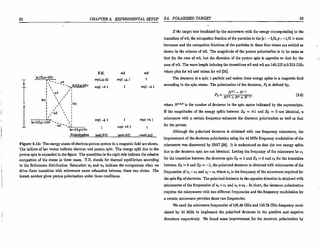
N t -NI _, eWXB7 - e-W">T jAg\ N1+Nl~ e*EWBT + e-*E/2kBT ~ t a m \2kBTj ' ( 7 )
where ks and T are the Boltzmann constant and the temperature, N f and N 4- are the number of protons or electrons with +1/2 and -1/2 spin along the magnetic field respectively. If we use 1 K° for temperature and 5 Tesla for magnetic field into Equation (3.7), we obtain the polarization of about 0.5% for proton and 100% for electron. We call this polarization due to the energy split as polarization at thermal equilibrium.
This proton polarization at the thermal equilibrium is not sufficient for the polarized proton target and we need introduce the DNP method. The basic idea of the DNP method is to utilize the high electron polarization to improve the proton polarization.-by using microwave.
Figure 3.15 shows the four energy states of four combinations of proton and electron spin in a magnetic field. The occupations for these four states at thermal equilibrium are shown in the column labeled as TE. wl, w2, w3, and w4 indicate the transition between the two states as shown in the figure.
If the target was exposed to the microwave with the energy corresponding to the transition w3, the electrons and protons in the |e *. —1/2, p : —1/2 > state are carried into the |e : 1/2, p : 1/2 > state. The electrons and protons in |e : 1/2, p : 1/2 > state falls into |e : -1/2, p : -1/2 > or |e : -1/2, p : 1/2 > states thermally. Because the transition w4 is even slower than the transition w3 or wl [20], the occupation fraction of the electrons and protons in the |e : -1/2, p : 1/2 > states increases and the occupation fractions of the electrons and protons in these states are settled as shown in the column of w3. As the result, the proton polarization is improved to be tanh(A/2) corresponding to the electron polarization in thermal equilibrium, instead of tanh(o"/2).
52 CHAPTER 3. EXPERIMENTAL SETUP 3A- POLARIZED TARGET 53
le:l/2,p:-l/2> I s - -.» w4
\ \
! X I / *
T.E. exp(-A-5)
w3 w2 exp( -A ) 1
1 exp( -A)
I J i /
'w3
le:-l/2,p:-l/2> - - . . \ w<C - - O
Wl
exp( -8 )
Ie:-l/2,pil72> ' Polarization tanh(&2)
1 exp( +A) exp( +A ) •)
tanh(A/2) -tanh(A/2)
Figure 3.15: The energy states of electron-proton system in a magnetic field are shown. The indices of ket vector indicate electron and proton spin. The energy split due to the proton spin is expanded in the figure. The quantities in the right side indicate the relative occupation of the states in three cases. T.E. stands for thermal equilibrium according to the Boltzmann distribution. Saturation W2 and W3 indicate the occupations when we drive these transition with microwave cause relaxation between these two states. The lowest number gives proton polarization under these conditions.
If the target was irradiated by the microwave with the energy corresponding to the transition of w2, the occupation fraction of the particles in the |e : - l / 2 , p : -1 /2 > state increases and the occupation fractions of the particles in these four states are settled as shown in the column of w2. The magnitude of the proton polarization is to be same as that for the case of w3, but the direction of the proton spin is opposite to that for the case of w3. The wave length inducing the transitions w2 and w3 are 140.127 ±0.213 GHz where plus for w2 and minus for w3 [20].
The deuteron is a spin 1 particle and makes three energy splits in a magnetic field according to the spin states. The polarization of the deuteron, Pa is defined by,
Pd = - (3.8) N+l+N° + N-i'
where N±l,° is the number of deuteron in the spin states indicated by the superscripts. If the magnitudes of the energy splits between Sz = ±1 and Sz = 0 are identical, a microwave with a certain frequency enhances the deuteron polarization as well as that for the proton.
Although the polarized deuteron is obtained with one frequency microwave, the improvement of the deuteron polarization using the 44 MHz frequency modulation of the microwave was discovered by SMC [38]. It is understood as that the two energy splits due to the deuteron spin are not identical. Letting the frequency of the microwave be v\ for the transition between the deuteron spin Sz = l and Sz = 0 and u2 for the transition between Sz = 0 and Sz = —1, the polarized deuteron is obtained with microwaves of the frequencies of ue — v\ and ue — v% where ue is the frequency of the microwave required for the spin flip of electrons. The polarized deuteron in the opposite direction is obtained with microwaves of the frequencies of ve + V\ and ve + v^ . In short, the deuteron polarization requires the microwaves with two different frequencies and the frequency modulation for a certain microwave provides these two frequencies.
We used the microwave frequencies of 136.48 GHz and 136.78 GHz frequency modulated by 44 MHz to implement the polarized deuteron in the positive and negative directions respectively. We found some improvement for the deuteron polarization by

54 CHAPTER 3. EXPERIMENTAL SETUP
3-5% with this frequency modulation.[20]
Figure 3.16 shows the E143 polarized target system. Liquid helium kept the ammonia target and the super conducting magnet at 1 K°. The magnet produced 5.1 Tesla magnetic field around the target cell to align the nucleon spin. The target insert had four cells which were filled by ND3, NH3, empty (nothing in it), and carbon or aluminum. We can select one of cells on the beam line by using a mechanical control. Each target cell had a dimension of $25 • 30mm. The microwave was fed to the target cell through a pipe and horn from the top of the system. The power of the microwave was about 1 Watt at the target cell.
The target polarization was measured with Nuclear Magnetic Resonance (NMR). The NMR is induced by a oscillating magnetic field perpendicular to the static magnetic field, the super-conducting magnet in E143 target system. A small fraction of the nucleon in the material oscillates between the spin up and down states with a frequency of the oscillating magnetic field. This signal resonates at the frequency determined by the static magnetic field and the magnetic moment of the nucleus. This phenomenon is called as Nuclear Magnetic Resonance (NMR).
The NMR signal was measured by using the technique of the Q-meter. A coil made from Copper and Nickel was placed in each target cell perpendicular to the static magnetic field. When we induce the oscillating magnetic field by using this NMR coil, the inductance of the NMR coil is modified by the target material existing in the coil to be [39]
L(w) = Loll + 4miWu>) - ft»]), (3.9)
where w is the frequency of the oscillation magnetic field, L(w) is the inductance of the NMR coil at the given frequency, L$ is the inductance of the coil in the vacuum, JJ is the filling factor of the material in the coil, x*(w) and x"(w) is the real and imaginary parts of the complex susceptibility of the material. The x"(w) is related to the target polarization 1 Pt, by the relation of [39]
Pt = Krx»du, (3.10) Jo
3.4. POLARIZED TARGET 55
Microwave Input
NMR Signal Out
Refrigerator
To Pumps
l b ^ Frequency
Figure 3.16: The electron beam comes from the left side of the figure. The magnets induce the 5.1 Tesla magnetic field along the beam axis. We rotated the target system by 90° along the vertical axis in the investigation for the Aj_.

56 CHAPTER 3. EXPERIMENTAL SETUP
200 3 0 0 MHz Figure 3.17: The NMR signal of the thermal equilibrium for ND3 under 5.1 Tesla and 1 K measured by Q-meter circuit. It corresponds to about 0.068% polarization.
where K is a constant involving the nucleus property. The imaginary part of the inductance is the real part of the impedance of the coil. In the Q-meter, the circuit is driven by a constant current source and the variable capacitance is set to absorb the phase part of the impedance of the coil. Therefore, the voltage of the circuit of the Q-meter is proportional to the real part of the impedance of the coil and the variation of the x" with the frequency can be observed as the variation of the voltage of the coil. Figure 3.17 shows the NMR signal as a function of the frequency w for thermal equilibrium of ND3 target. This x" is zero for all frequencies except for a small band close to the resonant frequency as shown in Figure 3.17, thus the area of the NMR signal above the base line is proportional to the target polarization from the Relation (3.10). The target polarization in the experiment was calibrated by using this NMR signal of thermal equilibrium corresponding to 0.068%.
We used the enriched UN nucleus instead of the usual UN. While the UN nucleus has the magnetic moment equal to that for deuteron, the lbN has the magnetic moment equal to that for proton and the NMR signal does not overlap to that for the deuteron. We were then able to measure both polarizations for the deuteron and the nitrogen nucleus in
3.5. SPECTROMETERS 57
the target and the effect of the nitrogen polarization was corrected properly as discussed in Section 4.2.5 and in Appendix D.
3.5 Spectrometers
Figure 3.18 shows a schematic view of the spectrometers. There were two independent spectrometers to detect electrons scattered off the ND3 target. These spectrometers were located along an angle of 4.5° and 7° from the beam axis. We call these spectrometers the 4.5° and 7° spectrometers respectively. Both spectrometers had two bending dipole
TOP VIEW
ND3 Target
e Beam
SLAC E142/E143 Spectrometers Dlpole Magnets Hodoscope
Quadrupole
Dipole Magnets \^-~~~^r ~\ Hodoscope g>-gta»
SIDE VIEW (7°) Counter
ND3 5 R° 9.6° r^Z~Z vtipt-
ND3 5 R° ,*«^-.-v 1 T M r^Z~Z vtipt-
TBJ! 2 . I m ' fe^fHi J-.£[5P CJ_^-^ Floor
CJ_^-^ Floor
0 5 10 15 meter
20 r - "
25 " " " " 1
30
Figure 3.18: This figure shows horizontal and vertical views of the spectrometer layout. The scale shows the distance from the target in meter. The vertical view is the layout for the 7° spectrometer.
magnets. Bl and B3 have the length of 118 inch and B2 and B4 have the length of 136 inch. The central momenta for the spectrometers were set to 11.5 GeV/c and 12.5 GeV/c

58 CHAPTER 3. EXPERIMENTAL SETUP
for the 4.5° and 7° spectrometers. The two magnets in each spectrometer bent electrons in directions opposite to each other. This configuration,has a larger momentum acceptance compared to the configuration bending in same direction [40]. Figures 3.19 and 3.20 show the momentum acceptance. The momentum acceptance of 4.5° and 7° spectrometers was from 6 and 7 GeV/c to beyond 20 GeV/c. respectively. The quadrapole magnet in the 4.5° spectrometer enhances the position dependence of electron momentum on the vertical axis and spreads electrons onto a larger detector area along the horizontal axis.
IS" 0.2
CD 0.1
o o CO
E142 DQD 4.5° Spectrometer
5 1 0 1 5 20 &£« MOMENTUM (GeV/c)
Figure 3.19: Momentum acceptance of the 4.5° spectrometer: the horizontal axis shows the momentum, the vertical axis shows the solid angle of the spectrometer acceptance. The solid line shows the solid angle of the acceptance of the E143 4.5° spectrometer. We indicate the acceptance of SLAC 20 GeV/c spectrometer by the half-dashed rectangle in contrast to the E143 spectrometer.
0.8 (m
s
0.6
ANG
LE
0.4
SOLI
D
0.2
0
1M1 7W2«
1 1 1 SLAC8GeV/c E142 00 Spectrometer 7° Spectrometer
N ^ ~ — ^ ^
• l ! / i! / '
\ \ / / \ i / / \ E130 DD
1 / ' \ Spectrometer " / ' \ / ' V
i / / \ '.ill \ \ i ! / i \ \ ! / ' \ . i / l , \ 7 1 \ 10 15 20
MOMENTUM (GeV/c)
Figure 3.20: Momentum acceptance of the 7° spectrometer: the horizontal and vertical axes indicate the momentum and the solid angle of the spectrometer acceptance respectively. The solid line shows the solid angle of the acceptance of the E143 7° spectrometer. We indicate the acceptance of the E130 spectrometer and the SLAC 8 GeV/c spectrometer by the dashed line and the half-dashed rectangle respectively in contrast to the E143 spectrometer.
A large photon background from the bremsstrahlung, pion decays etc. were expected at the small scattering angles. The spectrometer suppressed the photon background
3.5. SPECTROMETERS 59
Figure 3.21: Electron trace on the 4.5' F i g u r e 3 , 2 2 : E l e c t r o n t r a c e i n t h e 7 ° spectrometer: (a) is on the bending plane, spectrometer: (a) is on the bending plane, and (b) is on the horizontal plane. The a n d ( b) i s o n t h e horizontal plane. The traces are drawn for various momenta t r a c e s a r e d r a w n f o r v a r i o u s omenta from 7.5 GeV/c to 19 GeV/c. Note that f r o m 7 G e V / c t o 1 9 G e V / c - N o t e t h a t t h e
the figure's geometry is distorted so that fiSure's S«™etry is distorted so that the the trace of a 10 GeV/c electron at the t r a c e o f a 1 0 G e V / c e l e c t r o n a t ** c e n -center of the acceptance appears as a t « of the acceptance appears as a straight straight line. I l n e '

60 CHAPTER 3. EXPERIMENTAL SETUP
with the two bounce system [40]. In this system, the magnets and the collimators were
located such that the photon must hit those at least twice to reach the spectrometer
acceptance.
£
Is 84
S3 I s 2
1 -
\Ax/x = 0.1
Shower energy
7°-tracking ^" ^'" 4.5°-track!ng
v 6 8 10 12 14 16 18 20 22 24 momentum(GeV/c)
Figure 3.23: The dotted and dashed lines show the fractional momentum resolution for the 4.5° and 7° spectrometers respectively. The solid line shows the momentum resolution by the energy measurement with the lead glass shower counter. The small dashed line indicates the resolution corresponding to 10% error of Bjorken x.
Figures 3.21 and 3.22 show the ray-traces for the 4.5° and 7° spectrometers. Note that the figure's geometry is distorted so that the trace of a 10 GeV/c electron at the center of the acceptance appears as a straight line. In this configuration, we set the magnet layout to measure particle momenta from the trajectory gradients with largest possible acceptance. The momentum resolution of this configuration is worse than that for the same bending configuration, but it is acceptable for the experiment. Figure 3.23 shows the expected momentum resolution for each spectrometer and the momentum resolution coming from the requirement of Ax/x. The small dashed line in Figure 3.23 shows the momentum resolution to this requirement. The momentum resolutions of the 4.5° and 7°
3.5. SPECTROMETERS 61
spectrometers by the tracking shown by the dotted and dashes lines in this figure satisfied the requirement except in the high momentum region. It may be critical to the binning for the data in the high x region and will be studied in Section 5.6.3.
The several detectors were located after the bending magnets to detect electron tracks as shown in Figure 3.18. The detector systems are identical for both spectrometers composed of two threshold Cerenkov counters, seven hodoscope planes, a lead glass shower counter, and two scintillation trigger counters which will be explain in the following sections.
3.5.1 Cerenkov counter
Two threshold type Cerenkov counters were set in each spectrometer to identify electron tracks. Because electrons and pions give different momentum thresholds for emission of the Cerenkov light, we can identify the incident particle by measuring the Cerenkov light in the momentum region above the threshold. The signals obtained from the Cerenkov counter was used as one of the online trigger signals.
Cerenkov light is emitted when a charged particle passes through a medium faster than the light speed in the medium. The Cerenkov light is emitted in a cone of angle 0 which is given by
cos9=~, (3.11)
where, n is the refractive index of the medium, 0 is the relativistic 0 function. If 1/nfi is larger than 1, the Cerenkov photon is not emitted. Defining that d is the light speed in the medium and v is the speed of the particle, the Equation (3.11) is rewritten by
c o s 0 = - , (3.12)
From Equation (3.12), the Cerenkov light is often understood in the analogy of the shock
wave emitted by the object moving with the ultrasonic speed.
Since the /? of the high energy electron with a few GeV/c momentum is extremely
close to 1.0, the high energy electron in a medium always emits the Cerenkov light to

62 CHAPTER 3. EXPERIMENTAL SETUP
the direction of angle, arccos(l/n), from the track. In order to implement the electron-pion separation, we have to chose a medium which gives nff > 1.0 for electrons and nP < 1.0 for pions in the experimental momentum region. If we want the separation up to 13 GeV/c of the momentum, the refractive index of the medium, n has to be less than 1.000058 because 13 GeV/c pion has 0 = 0.9999424. In such a medium, only the electron emits the Cerenkov light for the momentum lower than the threshold, 13 GeV/c.
Figure 3.24: Schematic view of Cerenkov counter C2. The cylindrical tank was filled with depressured N2 gas. Cerenkov photon emitted by the incident electron tracks were reflected by three mirrors and focused on the photo-tube.
The two Cerenkov counters are made of aluminum cylinders placed along the spectrometer axis. The dimensions of the cylinders are 400 cm in length by $160 cm for the long counter (Cerenkov2, C2), 200 cm by $118 cm for the short counter (Cerenkovl, CI). To minimize <?-ray production and multiple scattering, the aluminum window of 1 mm thickness was used.
We used N 2 gas as the medium. Since the N 2 gas produces scintillation light as
3.5. SPECTROMETERS 63
well as Cerenkov light for charged particles, pions below the Cerenkov threshold produce light. However, the N2 gas has a good transparency at UV region, down to 150 nm wave length, and with use of the wave-length shifter, we improved the S/N ratio for Cerenkov light and the detection efficiency for electrons.
The Mirrors were placed at the end of the cylinder to collect Cerenkov photons to the photo-tubes. C2 had 3 mirrors which cover an area of 65 cm by 115 cm. CI had 2 mirrors which cover areas of 40 cm by 51 cm and 38 cm by 51 cm for the 4.5° and 7° spectrometers respectively. All mirror surfaces were coated with aluminum and MgP2
to optimize the mirror reflectivity. We obtained 90% of the reflectivity for 200 nm light. These mirrors were aligned properly by survey measurements using a solid state laser together with a simulation [41].
We used photo-tubes, Hamamatsu R1584-01 with UV glass window which have the large diameter and high quantum efficiency. The surfaces of the photo-tubes were coated with wave length shifter of 2430 nm thickness of para-terphenyl and overlayed with 25 nm thickness of MgF2 to protect the wave length shifter against evaporation and aging.
The refractive index for a given gas pressure is given by using Lorenz-Lorentz relation [41],
$ $ ^ = *(A)p, (3.13)
where n(A) is the refractive index at wave length A, p is the density of the gas, and K is a constant, 0.163cms/s for N2. The pion thresholds of the Cerenkov counters were set at 13 GeV for C2, and 9 GeV for CI. These pion thresholds correspond to N 2 pressures of 240 mmHg and 500 mmHg for the C2 and CI respectively. Coincidence of these short and long Cerenkov counters selected electron tracks and rejected pion tracks cleanly because only a few % of pion emit scintillation light. The purity of the electron sample was estimated to be more than 99% from the study for the experimental data.
The number of photons by the Cerenkov emission is expected by the following formula [42],
N = 27raLsin2B J** ^d\ (3.14)

64 CHAPTER 3. EXPERIMENTAL SETUP
where a is the fine structure constant, L is the length of the medium, 0 is the Cerenkov angle, and Ai and A2 are the lower and upper limits for the sensitive region in the wave length. If we assume the sensitive region of the PMT between 150 nm and 550 nm in the wave length, the refractive index n is 1.000058, the length of the counter, L, is 4 m, the number of the Cerenkov photon is expected to be 106. Actually, the number is reduced due to the transparency of the N? gas, the mirror reflectivity, and quantum efficiency of the photo-tube, etc. Including these reduction factors, the number of the Cerenkov photon was estimated to be 8.2 ± 0.5 by a Monte-Carlo simulation [41].
Detection efficiency
The detection efficiencies of the Cerenkov counters were studied under an assumptions that the probability of detecting photo-electrons (Cerenkov ADC count) is Poisson distribution [41]: Table 3.1 shows the efficiencies defined to be the probability to produce one or more photons which was evaluated from the Cerenkov ADC spectrum. All of these
4.5°. 7°. CI C2 CI C2
Mean ADC Npe
Eff.
165.6 ±56.6 8.6 ±0.5
99.98± < 0.01
127.1 ±42.3 9.0 ±0.5
99.99± < 0.01
158.8 ±54.2 8.6 ±0.5
99.98± < 0.01
137.2 ±55.5 6.1 ±0.5
99.78± < 0.11
Table 3.1: Cerenkov counter efficiency from ADC spectra.
counters have high detection efficiencies of more than 99%. The numbers of Cerenkov photons Npe were evaluated from the ADC spectra close to the value of 8.2 ±0.5 obtained from the Monte-Carlo simulation.
3.5.2 Hodoscope
There were seven plane hodoscopes on each spectrometer. The purpose of hodoscope
systems was to reconstruct charged particle tracks. A track is used to determine the
3.5. SPECTROMETERS 65
particle's momentum from the reverse matrix of the spectrometer magnet. A hodoscope was assembled with finger scintillation counters which were placed
parallel to each other so that hits on the finger of the hodoscope gave the information on the track position in the transverse direction with respect to the finger axis. Every finger overlapped its neighbor finger by 2/3 of its width as shown in Figure 3.25. This configuration improved the effective spatial resolution of the hodoscope allowing a time coincidence measurement between fingers overlap.
Figure 3.25: Finger overlap: The di- Figure 3.26: Hodoscopes schematic mension is of H1U hodoscope. view: the first set was composed by four
hodoscopes which determined position of tracks in u, x, y, y axes. The second set was composed by three planes which determined position in x, y, u axes. C2 counter was located between H4Y and H5X planes.
The seven hodoscopes were located along the spectrometer axis in order of H1U, H2X, H3Y, H4Y, H5X, H6Y, and H7U as shown in Figure 3.26, where X,Y, and U correspond to the x, y, and diagonal measurement of the track position respectively. The planes 1 through 4 were between Cerenkovl and Cerenkov 2, and planes 5 through 7 were between Cerenkov 2 and the shower counter.
Table 3.2 and 3.3 show the dimensions of the finger scintillators of the hodoscopes

66 CHAPTER 3. EXPERIMENTAL SETUP 3.5. SPECTROMETERS 67
in the 4.5° and 7° spectrometers. Table 3.4 lists the ringer lengths for the U hodoscope. H2X, H3Y, H5X, and H6Y had a higher spatial resolution than others and therefore these hodoscopes dominated the momentum resolution of the spectrometer. HIU, H4Y, and H7U had a roll to improve the signal purity and reliability and to remove any accidental double hit. H2X, H3Y, H5X, and H6Y were built by Syracuse group originally for E142 which investigated deep inelastic scattering of the electron with gas 3He target [23]. H4Y was built by SLAC, and H7U by French group for E142. HIU was built by TOHOKU group for E143.
Plane width(mm) length(mm) thickness(mm) number HIU H2X H3Y H4Y H5X H6Y H7U
45 20 30
47.6 30 30 75
Various 590 430
355.6 1070 510
Various
6.2 6.2 6.2 6.2 6.2 6.2 10
25 34 31 20 27 55 21
Total finger number 213
Table 3.2: Hodoscope dimensions on 4.5° spectrometer.
Plane width(mm) length(mm) thickness(mm) number HIU H2X H3Y H4Y H5X H6Y H7U
45 30 30
47.6 30 30 75
Various 690 430
482.6 1070 510
Various
6.2 6.2 6..2 6.2 6.2 6.2 10
25 23 36 20 27 55 21
Total finger number 207
Table 3.3: Hodoscope dimensions 7° spectrometer
HIU H7U length (mm) number length(mm) number
200 260 320 380 440 500 560 620 680 720 740
2 2 2 2 2 2 2 2 2 1 6
200 300 400 500 600 700 760 820
2 2 2 2 2 2 2 7
Total 25 Total 21
Table 3.4: U-hodoscope dimensions
High voltage modules were located in the counting house located upstairs of ESA. We stretched more than 120 SHV coaxial cables from the counting house into ESA to supply high voltages' for these photo-tubes. To reduce the number of the SHV cables from the counting house to ESA, we used high voltage splitters in the spectrometer. One long SHV cables provided high voltage for up to four photo-tubes. Figure 3.27 shows the circuit of the splitter; where the voltage was determined by a ratio of the variable resistance to the inner resistance of the photo-tube.
A photo-tube detected a signal from a single finger. Photo-tubes which were used for all hodoscopes except for the HIU plane are specified in Reference [23]. The phototubes for the HIU plane were H3167 by Hamamatsu. This photo-tube has a f inch diameter, a length of 103 mm, a sensitive region of 300 - 650 nm in the wave length, a gain of 2.0 x 10⁶ and a rise time of 1.8 ns at -1.5 kV. The upper limit for the high voltage is -1.9 kV. The scintillator used for the HIU plane is SCSN38 by Kuray which has a density of 1.05g/cm3 and a refractive index of 1.59. The scintillation light wave length

68 CHAPTER 3. EXPERIMENTAL SETUP
Variable resistances outputs
input
t -AAAr
AA/V
Figure 3.27: Hodoscope High voltage splitter. Only two of the four outputs are drawn.
distributes from 400 beyond 500 nm.
The output signals of the photo-tube was processed by a LeCroy 4413 discriminator mounted in two CAMAC crates in each spectrometer-hut. The threshold was -30 mV for H1U and -50 mV for the others. Output ECL signals with 20 ns width were sent to the counting house by twisted pair cables. Bach signal went to a LeCroy 2277 TDC through a gate-card which ignored any signal when the input gate was closed. The gate was called as Hod-gate made by trigger logic which fired for passing charged particles. The LeCroy 2277 TDC recorded up to 16 signals for each channel. The resolution of the TDC is 1 ns and the TDC buffer is 16 bit for each signal. Therefore the dynamic range is 65/JS. Because the spill width was about 2.2/is in length, this dynamic range is enough to record the hodoscope hits for a spill.
timing calibration
The timing at each hodoscope was obtained by comparing the measuring timing with the expected timing of the reconstructed track passing through the hodoscope. Where the track reconstruction was performed by using information from the hodoscopes, the Cerenkov counters, and the shower counter. The procedure of the track reconstruction will be described in Section 4.1.3.
We first take time difference between the measured timing and the expected track
3.5. SPECTROMETERS 69
Sp4iklo
Spilhlx
SjvtiMj
Sp4:hif
. Sp4ih5x J I um : fl MM*
MM i r \ a *"* S •x. U M
a
• Sp4iMy „
1 / { in*
• Sp4 lh7u —
[ MM " J V
Figure 3.28: The spectra of At of the hodoscopes for the 4.5° spectrometer after the calibration. The time difference between the hodoscope hits and the reconstructed tracks are plotted. The results from fingers are accumulated together about a hodoscope plane.

70 CHAPTER 3. EXPERIMENTAL SETUP
mm . Sp7ih5x it mm ! r n • M : i I
3 -8 J -• «
1 »« s
Sp7iWj
\ , • Sp7lk7o n «#
/ " i MM } i ? J • 1 4 1 1
Figure 3.29: The spectra of the At for the 7° spectrometer after the calibration. The time difference between the hodoscope hits and the tracks are plotted. Results from fingers are accumulated together about a hodoscope plane.
3.5. SPECTROMETERS 71
timing at a given hodoscope as follows,
&t={tm-td-tp)-trec (3.15)
where the tm is the TDC count of the hodoscope fingers, the U is the propagation delay of scintillation light in the hodoscope finger, the tp is the TDG pedestal including the time delay due to the electric line, and the trec is the timing of the reconstructed track passing the finger.
The propagation delay in the scintillator was calculated from the hit position and the propagation speed in the scintillator. The hit position on a finger was determined taking a time coincidence with another finger crossing to the finger. The propagation speed for each finger was calculated from E142 run as nearly equal to 15 cm/ns [23].
We tuned the At spectrum to center at 0 by adjusting the TDC pedestal tP with iteration procedure. Figures 3.28 and 3.29 show the spectra of the At for the 4.5° and 7° spectrometers after several iterations. We plotted only the hits used for reconstruction of tracks. All hodoscopes were well calibrated resulting the sharp peaks at zero. Table 3.5 shows the time resolution of the hodoscopes evaluated from these plots. The time resolution of about 1 ns was obtained for all hodoscopes.
Plane time resolution (ns) for 4.5° sp. time resolution (ns) for 7° sp. H1U 1.18 1.14 H2X 0.90 0.74 H3Y 0.72 0.93 H4Y 0.88 0.89 H5X 0.77 0.75 H6Y 0.69 0.77 H7U 1.05 1.04
Table 3.5: Time resolution of the hodoscopes

72 CHAPTER 3. EXPERIMENTAL SETUP
Hodoscope efficiency
We calculated the detection efficiency of the hodoscope defined by the probability to make hits for passing tracks.
The track was reconstructed by a fitting as described in Section 4.1.3. To improve the reliability for the track sample, we required,
1. Both Cerenkov counters have hits in the trigger,
2. Six planes of the seven hodoscopes have hits,
3. Spatial matching between the shower cluster and the track within 20 mm,
4. The track was reconstructed within 10 mm from the target center.
To ignore the effect of the finite spatial resolution of the tracking giving the improper finger address, we accepted the event when any finger within the width plus 50 mm from the track position has a hit.
Figure 3.30 and 3.31 show the inefficiency for the hodoscopes in the 4.5° and 7° spectrometers respectively for run 1334. Horizontal axis shows the hodoscope plane index from 1 to 7. Vertical axis shows the inefficiency of each plane in logarithm scale.
3.5.3 Shower counter
The shower counter was placed at the end of the spectrometer to measure energy of the electron. The shower counter is a multi-segment electro-magnetic calorimeter built with lead glasses. High energy electrons incident to the lead glass induce an electro-magnetic shower due to bremsstrahlung and pair creation and produce a large number of electrons, positrons, and gammas. These electrons and positrons lose their energy ionizing atoms and emitting Cerenkov light in the lead glass. The total amount of the Cerenkov light is proportional to the total path length of the electrons and positrons in the shower counter which is proportional to the initial energy of the electron [42], thus the shower counter
3.5. SPECTROMETERS 73
• i , . . . i 1 2 3 4 5 6 7 1 2 3 4 5 6 7
plane number plane number
Figure 3.30: Plane inefficiency for run Figure 3.31: Plane inefficiency for run 1334 in 4.5° spectrometer 1334 in 7° spectrometer
measures the energy of the electron by collecting the Cerenkov light in the lead glasses with photo-tubes.
The counter was built with 200 lead glass blocks of 62 • 62 • 750mm as shown in Figure 3.32. The radiation length of the lead glass is 3.7 cm. Because the 750 mm lead glass corresponds td 24 radiation length, electrons lose more than 99.9% of the energy in the lead glass.
The output from each photo-tube was divided into five line as shown in Figure 3.33. These four lines went to ADC via 200 ns delay line. Each ADC channel was able to collect a datum once in a spill of 2.2 JUS because we read and initialized the ADC buffer after every spill. Thus, we were able to collect the data up to four times in a spill. Each four of the fifth line were summed and divided into two lines. One of them was sent to TDC via a discriminator to measure the timing of the signal. Another line was used to make the signal from the whole counter. This signal from the whole counter made one of online electron trigger signal as will be mentioned later.
There were three purposes for the shower counter; (l)providing online electron trigger signal, (2)measuring the electron energy, and (3)particle identification using a
IT1'-
ur3-
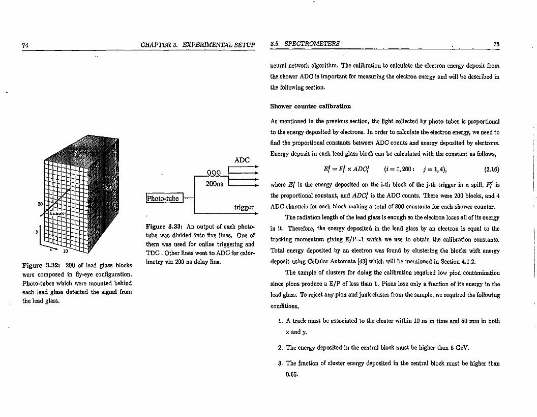
74 CHAPTER 3. EXPERIMENTAL SETUP
Figure 3.32: 200 of lead glass blocks were composed in fly-eye configuration. Photo-tubes which were mounted behind each lead glass detected the signal from the lead glass.
ADC
000 * •
000 ^ 200ns fc 200ns 200ns
Photo-tube
200ns 200ns
trigger •
Figure 3.33: An output of each phototube was divided into five lines. One of them was used for online triggering and TDC . Other lines went to ADC for calor-imetry via 200 ns delay line.
3.5. SPECTROMETERS 75
neural network algorithm. The calibration to calculate the electron energy deposit from the shower ADC is important for measuring the electron energy and will be described in the following section.
Shower counter calibration
As mentioned in the previous section, the light collected by photo-tubes is proportional to the energy deposited by electrons. In order to calculate the electron energy, we need to find the proportional constants between ADC counts and energy deposited by electrons. Energy deposit in each lead glass block can be calculated with the constant as follows,
E{ = F{ x ADC{ (£ = 1,200: i = l,4), (3.16)
where E\ is the energy deposited on the i-th block of the j-th trigger in a spill, F/ is the proportional constant, and ADC\ is the ADC counts. There were 200 blocks, and 4 ADC channels for each block making a total of 800 constants for each shower counter.
The radiation length of the lead glass is enough so the electron loses all of its energy in it. Therefore, the energy deposited in the lead glass by an electron is equal to the tracking momentum giving E/P=l which we use to obtain the calibration constants. Total energy deposited by an electron was found by clustering the blocks with energy deposit using Cellular Automata [43] which will be mentioned in Section 4.1.2.
The sample of clusters for doing the calibration required low pion contamination since pions produce a E/P of less than 1. Pions lose only a fraction of its energy in the lead glass. To reject any pion and junk cluster from the sample, we required the following conditions,
1. A track must be associated to the cluster within 10 ns in time and 50 mm in both x and y.
2. The energy deposited in the central block must be higher than 5 GeV.
3. The fraction of cluster energy deposited in the central block must be higher than
0.65.

76 CHAPTER 3. EXPERIMENTAL SETUP
4. Classified as an electron by the neural network.
Lead glass blocks are classified as shown in Figure 3.34. The first category is "non-edge block" which means not on the edge of lead glass array. The second is "edge-block" which has only three adjacent blocks. Last one is "corner block" which has only two adjacent blocks. Sometime we call a cluster whose center is on a non-edge (edge, corner) block as a non-edge (edge, corner) cluster. The calibration was done with different ways for these three classes of blocks.
H t t i i t t • JtyivwA 1!^!?^ m i
Non-edge
Figure 3.34: Classification for the shower block (cluster)'
The electron energy is mostly deposited in the center block and spread over the surrounding eight blocks [44]. Hence, we required that the total energy deposited in these nine blocks gives E/P = 1 for the non-edge cluster. The constant for the block was corrected after every iteration by the averaged E/P as,
where F/ is the constant for the i-th block and j-th ADC channel, < E/P >{ is an averaged E/P which was taken at this iteration, (Fi)prime is a new constant.
For the edge clusters, we can not require E/P to be 1 because a part of electron energy escapes out of the counter. However, the edge block and its adjacent five blocks are supposed to occupy a certain fraction of the energy deposit with respect to the total energy of electron. This fraction was estimated from the well calibrated non-edge block
• S B -
Edge
Is mm
Comer
3.5. SPECTROMETERS 77
data as 0.92 [44]. Hence, the constant for the edge block was calibrated by
(F/)< = ° - 9 2 i ? < Eedse6/P >i
(3.18)
where the < Eedgee/P >{ is defined similar to that for the non-edge cluster but the total energy deposited of the six blocks.
The edge block was calibrated also with a energy fraction to the total energy deposit when an electron passed through the adjacent block. It was estimated to be 6.5% [44] and we corrected the constant by
1 , ; <Eedge/P>\ (3.19)
In these two correction method for the edge block, we selected which gave a smaller correction than the other to prevent the divergence of the constant due to the statistical fluctuation.
The corner block was calibrated using a energy deposited in the corner block by an electron passing through the inside diagonal block. The ratio of the energy deposit to the electron momentum, 2?Cwner/-F> was studied to be 2% [44]. We corrected the constant by
0.02F/ (F/)' = (3.20) < Ecomer/P >f
Table 3.6 shows the results of the shower calibration. Each run corresponds to a typical run of a run block which was a bunch of runs classified due to some hardware changes.
run # < E/P > 4.5° < E/P > 7° 1560 1.000 ± .054 1.000 ±.057 2750 1.000 ± .054 1.001 ± .059 2926 1.000 ±.055 1.000 ± .060
Table 3.6: E/P after the calibration. The error is the standard deviation of the distribution of E/P.

78 CHAPTER 3. EXPERIMENTAL SETUP
3.5.4 Trigger counter
Discriminator Coincldenced output
Figure 3.35: Front trigger counter: Fish-tale acrylic light guides introduced emitted photons into the photo-tubes. Two outputs on a side was combined linearly by a linear Fan-in. Then these signals are discriminated by 30 mV threshold. The coincidence of the outputs was sent to the trigger electronics. Outputs of the Fan-ins were also recorded by TDC independently.
E143 spectrometer had two scintillator trigger counters. The front trigger counter was set between Cerenkov counter 1 and Hodoscope H1U plane. The dimension of the counter was 700 • 450 • 6 mm as shown in Figure 3.35. The scintillator was made of Kuray SCSN38 with higher photon emission than for Bicron [45]. We used the photo-tube Hamamatsu H3690 which has a dimension of $lg inch x 113 mm, a sensitive region of 300-650 nm in the wave length, a current gain of 5.3 x 10⁶ and a rise time of 2.0 ns at -1.5 kV. The limit of the high voltage is - 1.9 kV. Figure 3.35 shows the assembly of the photo-tube and the scintillator for the front trigger counter. These photo-tubes were connected through light-guides to the scintillator.
The rear trigger counter was placed between Cerenkov counter 2 and Hodoscope H5X plane. The scintillator was Kuray SCSN38 with the dimension of 1100 • 550 • 13 mm. Signals were read out by two photo-tubes through the twisted acrylic light guides
3.5. SPECTROMETERS 79
attached at each end of the scintillator. The photo-tubes were Hamamatsu H1161 of <£60 mm diameter with the sensitive wavelength from 300 to 650(nm). The current gain is 5.3 x 10⁶ and the rise time is 2.6 ns at -2.0 kV.
Output Discriminator
Figure 3.36: Rear trigger counter: The outputs from both sides were processed by a discriminator with 50 mV threshold. The coincidence of these signals was used as one of online trigger signal. Each outputs were recorded by TDC.
The coincidence of these front and rear scintillation trigger counters were used as an online trigger with a rate suppressed by a pre-scaler. The signal served as the hodoscope gate and the trigger for pions which will explained in Section 3.5.5.
Cosmic ray test
The time resolutions of the scintillation trigger counters were measured with the signal produced by cosmic-rays [46], Figure 3.37 shows the location of the investigation. A coincidence of two scintillation counters, counter A and B, each having an area of 5 • 5 cm defined the timing and location of the passing of a cosmic-ray. The signals from the photo-tubes of both sides of the front trigger counter were processed by discriminators and a mean timer. The mean timer gives an averaged timing of two input signals by,
'W — o \rtdi, (3.21)

80 CHAPTER 3. EXPERIMENTAL SETUP
Cosmic ray
! ^ \ S ^ ^ Counter A
Counter B
Figure 3.37: Setup of the time resolution measurement: Counter A and B are scintillation counters which have the dimension of 50 • 50 • 20mm. The coincidence of these counters defined the passing of cosmic ray.
I' ZfiUUt 4135 UtOA 0 97MC-OI RUS 0 8407 AUCHAM 4131. xy*«r»2.2j / « ComicM 421.71 8815 utat O.I15I i O.1204C 01 S'*m» 0 7642* osatee 01
Ctl .A-front trifftr
Figure 3.38: Time difference between counter A and the front trigger counter.
3.5. SPECTROMETERS 81
where IM is the mean timer output, *i and t2 are the timing of the inputs, and t&i is the delay time of the circuit. We used the mean timer instead of the coincidence to compensate the timing shift due to the propagation of photons in the scintillator. The time differences of the three combinations among counter A, B, and the front trigger counter were recorded by TDC with 25 ps/channel. Dividing the area of the front trigger
5MO
i
!
10 32 DtlrStf 4138 Utort -0.8S12C-O1 ftUS 0.4909 AU.CKAN 4138.
fc700
!
XVntff 127.6 J 17 COMtflM 8 7 9 . f l 14.28 Uion - 0 M * t C - O I ± 0-7473C-02 Sl«mo 0 47041 0 « » i r - 0 2
500 ! 400 • M 0
200 }
too • J ' . . . i . . . i . r . . i . ! L i . . . i . . . i . . . t . . . i
Crttrf*! 4138 M«n -0.1733 RUS 0.8644 AUCKAM 4133. XYftdf92.il / 40 Conitont 407.3 * 8.371 U(4t -0.1801 * 0.1253C-01 Slstio 0.7010* 0.103HC-01
Figure 3.39: Time difference between counter A and counter B.
Figure 3.40: Time difference between counter B and the front trigger counter.
counter into three by three, we took the data at the divided nine points of the counter. Figure 3.38, 3.39, and 3.40 show the time differences. These histograms contain all of data which were taken at the nine points. The resolution of these distributions come from the intrinsic time resolutions of these individual counters. Thus, for example, the resolution in Figure 3.38, ad, can be written by
<Jd = \ M + < 'F> (3.22)
where a A and ap are the resolution of counter A and the front trigger counter respectively. Therefore, we calculated the intrinsic time resolutions for these three counters from these three distributions. The intrinsic time resolution of the front trigger counter was obtained to be 0.71 ns.

82 CHAPTER 3. EXPERIMENTAL SETUP
t
|JSO
300
250
200
: 1 10 21 Ertlriti 3 « i Uwrt - 0 2007 BUS 0.7 J11 : 1 COAIIOM J 4 9 « 4 fl«0 U«Krt -Q. I64»± O.I147C-01 Sfcmo ©6*0J± 0 » 7 « C - 0 I
: 1 '. 1 1
1 1 \ j \ 1 . J.....I. I . . . I • • • • * • • '
0»f.A-fltOft/^J»r
Figure 3.41: Time difference between counter A and the rear trigger counter
I L io u Cnlrfu M l M M A - 0 . 1 U 0 C - 0 I RUS 0837ft I L X*/fUf 114.7 / 4» Cwutttt 399.01 9.077 WMft - O . W M E - 0 1 * 0.1150C-01 S ima O i S U i O9U7C-01
\f[ ' - - I . . . . . . . I . . .
tO 12 14
Off. 0 - R#4r \*ntt
Figure 3.42: Time difference between counter B and the rear trigger counter.
Similarly, the resolution for the rear trigger counter was obtained from Figure 3.41 and 3.42 to be 0.56 ns.
3.5.5 Trigger electronics
E143 spectrometer system opened the gates for TDC and ADC whenever a trigger signal was generated. This trigger signal was generated independently in the 4.5° and 7° spectrometers. The number of the gate for the ADC and the hits for the TDC were limited up to four and sixteen, or less respectively in a spill. The number of electrons in a spill is typically one or less, on the contrary, the number of pions was higher than that for electrons. Thus, we imposed the following requirements for the trigger electronics for the efficient measurements of electrons and pions:
1. Open the ADC and TDC gate for all electrons,
2. Open the ADC and TDC gate in a fraction of times for pions to prevent the trigger burst by many pions.
Figure 3.43 shows the basic picture for the E143 trigger electronics. Basically, the passing
3.5. SPECTROMETERS 83
h electron)
cjdfoion -H pion-or 1 h electron)
cjdfoion -H pion-or 1
F*-> main-or — • A D C - * • main _r
electron
4 4 hod-gate ^ mry* *
hod-gate
Figure 3.43: Basic idea of the E143 trigger logic: the main and pion-or triggers are generated when electrons and any charged particles pass through the spectrometer respectively. The "or" product of the main and pion-or triggers composes the main-or trigger which opens the ADC gate. The hod-gate trigger which opens the TDC gate is generated also when electrons and charged particles pass the spectrometer. The rate for the charged particles ( not for electron) is suppressed by different factors for pion-or and hod-gate triggers.
of electrons and any charged particles are defined by the coincidence signal of the two Cerenkov counters and the two scintillator trigger counters respectively. The "or" product of the two coincidence signals composes the main-or trigger which opens the ADC gate and the hod-gate trigger which opens TDC gate. The difference of these trigger signals is the suppression factor for the coincidence signal for the scintillation trigger counters. This suppression is to prevent the trigger burst by many pions and the difference of the suppression factors is because of the acceptance of the number of signals of the ADC and TDC in a spill.
Figure 3.44 shows the logic of the main trigger and the other coincidenced signals in detail. SI and S2 are the output signals from the front and rear trigger counters after processed through discriminators. HodSum is the logical sum of the output signals from all fingers of H2X hodoscope. The coincidence of 51,52, and HSUM generated SciCoin. The rate of the signal was reduced by a pre-scaler with a factor N4 in order to prevent the trigger burst by many pion tracks. This pre-scale factor N4 was normally set to 4 for the 4.5° spectrometer and 1 for the 7° spectrometer.

84 CHAPTER 3. EXPERIMENTAL SETUP
SI
S2
Hod Sum
CI
SI
S2
Hod Sum
CI
r—j p = •• S/N4 SI
S2
Hod Sum
CI
PS Fan out
BG
SI
S2
Hod Sum
CI 4= Dl
L_)M
scr. BG m—*- S/N4.C2-M
SI
S2
Hod Sum
CI 4= Dl
L_)M jw]
BG
SI
S2
Hod Sum
CI 4= Dl
L_)M Id I
BG
Fan out
Dl
L_)M IU.|
BG
fe
C2 A — I L < V " ' I m-+- CI.L,C2-L
C2 1= — \ k
j I • — » • C1-M.C2-M
— \ k
d.| IBGI ^
1 — • — > • Main Shw Sum
— \ k ow| ^ fc ShwSum VI Shw Sum - j i —(vT
— I M - j i —(vT
— I M d. I • ShwSum-M
Figure 3.44: The logic of the main trigger and the other triggers are shown. Si and S2 are signals from the front and rear trigger counters, HodSum is a sum of all outputs of the H2X hodoscope, Cl and C2 are outputs from the Cerenkov counters, ShwSum is a sum of outputs from the lead glass blocks, and BG is the beam gate opened whenever beam came into ESA. A black half circle is a coincidence and a gray circle is a pre-scaler to reduce the signal rate. The coincidence of the ShowSum, CI, C2, and BG composes the main trigger.
3.5. SPECTROMETERS 85
The Cerenkov counters are very important to identify electron tracks. The signals from these counters were processed through two discriminators with 30 mV and 50 mV thresholds. These signals were labeled as Cl-L, Cl-M for CI and C2-L.C2-M for C2.
The shower counter provided four ADC and one trigger signal as shown in Figure 3.33. One of those outputs was used to make shower trigger signal. This trigger signal is the sum of signals from all 200 lead glasses and processed through discriminators with three threshold levels. The signals corresponding to these threshold level are denoted very low, low, and medium and labeled by ShwSum-VL, ShwSum-L, and ShwSum-M.
The main trigger was the coincidence of Cl-L, C2-L, ShwSum-L, and beam gate which was open whenever beam came into ESA and sent from Linac Main Control Center (MCC). This main trigger provided information of the electron passing the counter for the online process. The rate of the main trigger was typically 1.5 for 4.5° spectrometer and 0.3 for 7° spectrometer per spill.
ShwSum-VL
SclColn ShwSum-L - ^
Bfir-fr-
E £ r - ^
S/N4.C1-M-S/N4.C1-M-C1-L.C2-L •
-••Honor
w-hod-gate
Figure 3.45: Logic of pion-or and hod-gate triggers is shown. The closed wedge-shape is the or logic. S/N4:Cl-M,S/N4:C2-M, and C1-L-.C2-L are given in Figure 3.44. The gray circles are the pre-scaler suppressing the signal rate.
Figure 3.45 shows the logic of the pion-or and the hod-gate triggers. The pion-or trigger was the trigger generated any charged particle including pion. These pre-scaler factors in the figure were set to 32 for 4.5° spectrometer and 8 for 7° spectrometer. Typically, the rate was 0.35/spill and 0.25/spill for 4.5° and 7° spectrometer respectively.

86 CHAPTER 3. EXPERIMENTAL SETUP
TDC recorded data for any hits of hodoscopes, shower counter, Cerenkov counters, and the other triggers when the hod-gate trigger was fired. Gate-card ignored ECL signals from the discriminator to TDC if the hod-gate was closed. The hod-gate was generated by or product of the SciCoin and the coincidence of the Cerenkov counters which is always enable to open the hod-gate for the electron.
ShwSum-M ^ _ S/N4.C1-M W
ShwSum-M ^ S/N4.C3-M | /
S/N4 | k C1-M.C2.M §r
ploiv-or
main
Figure 3.46: Logic of the main-or trigger which was generated by the main trigger which fired only for passing of electrons and the pion-or trigger which fired for the passing of charged particles. The main-or trigger opened the ADC gate for the shower counter and the Cerenkov counters.
Figure 3.46 shows the logic of the main-or trigger. The main-or trigger opened the ADC gate to record data for the energy deposit of the shower counter and spectra of the Cerenkov counters. The number of the main-or trigger was limited by the electronics of the shower counter up to four or less per spill by the electronics used for the shower counter. This trigger was primarily formed by the the main trigger and the pion-or trigger to record the electron data and the pion data reduced by pre-scaler.
3.6 Data acquisition and data handling
The experiment has been carried out from Nov. 1993 to Feb. 1994 at ESA of SLAC.
The Linac was operated at 120 Hz with a 3.0 • 109electron/spill current typically. Beam
energy was switched 10, 16, and 29 GeV to study the Q2 dependence of the structure
functions. Table 3.7 lists the run summary.
i^JB—•• eoaln-or
3.6. DATA ACQUISITION AND DATA HANDLING 87
Target field Energy (GeV) Target Beam charge (electrons • 1018)
Electrons (triggers • 106)
Longitudinal 29.13 NH3 130 39 Longitudinal 29.13 ND3 170 77
Longitudinal
16.20 NH3 37 11
Longitudinal
16.20 ND3 17 7.5
Longitudinal
9.8 NH3 19 6
Longitudinal
9.8 ND3 16 7
Transverse 29.13 NH3 56 17 Transverse 29.13 ND3 69 30
Either/none all C.Al.Empty 16 8 Total 2-10 8
Table 3.7: E143 data summary: The longitudinal and transverse target fields mean the direction of the target polarization with respect to the beam axis. The transverse asymmetry A±. was measured only for 29 GeV beam.
The data were processed in the counting house of ESA. Figure 3.47 shows the online control and the data acquisition system which was based on CAMAC system controlled by VAX4000.300. Three DEC3000.400 computers analyzed and monitored online data on network. A VAX station 4000.60 was used as a tape server to store the data in 8mm data tapes which can save up to 2.5 Giga bytes of information. We used about 300 tapes for E143.
The data were processed with a E143 analysis program. It was a hybrid program compiled from C and Fortran source codes. C codes served as the main routine for process communication, graphical interface etc. The main part of the physics analysis was coded by Fortran.
We analyzed the data stored of the 8mm tapes with a basic event reconstruction
process and stored the results in other 8mm tapes. The latter 8mm tapes were called
DST which stands for Data Summary Tape. The date size was reduced by a factor 4 in
the DST in contrast to the initial data. The physics calculation was done using the DST.

88 CHAPTER 3. EXPERIMENTAL SETUP
VAX 4000300 MonItor& Control
Monitors Control CAMAC
DEC3000.400 4.5Deg Analysis
UnlxWS Beam data Analysis
DEC30O0.400 4.5Deg Analysis
1 r,~~ | Bridge
>
Beam data CAMAC
VAX 4000300 Monitor* Control
4.5deg data CAMAC
Moller data CAMAC
7dcg. data CAMAC
ethemet
VS3100 FE Control
VS4000.60 Tape Server
|8mmMT|
Figure 3.47: Data acquisition and control system
The DST contained the following information:
1. beam spill data
(a) Pulse height of good spill monitor
(b) Pulse height of bad spill monitor
(c) Output of Toroid current monitor
(d) Beam position and width
(e) Electron beam helicity
2. timing of trigger signals
3. Track data
(a) track momentum
(b) track direction and position
3.6. DATA ACQUISITION AND DATA HANDLING 89
4. Cerenkov timing and pulse height
5. Shower cluster data
(a) Cluster centroid
(b) Cluster energy
(c) Neural network response
We made summary files from the DST. The summary file contained only the numbers of tracks binned in x and Q2 according to different definitions. These definitions are summarized to be
1. Basic electron definition, energy = shower counter deposit,
2. Basic electron definition, energy = track momentum,
3. No tracking (defined only shower cluster and Cerenkov),
4. Basic pion definition(No main trigger, no Cerenkov hits, neural network indicates
no electron), etc.

Chapter 4
Analysis
The purpose of this chapter is to describe the analysis to give the cross section asymmetries, A\\ and As. from the data of deep-inelastic scattering of the 29 GeV electrons off the deuterized ammonia target. These asymmetries are used to calculate the spin structure functions gi as mentioned in Chapter 2.
The event reconstruction and the particle identification to select a good electron sample will be explained first. Then, the calculation of the asymmetries from the obtained electron sample will be explained including the corrections for the asymmetry.
4.1 Event selection
4.1.1 Beam analysis
We required to record data from the good beam spills by excluding the unstable beam spills in the analysis for the cross section asymmetry. The beam stability were examined with several devices; good spill monitor, bad spill monitor, toroid current monitor, and foil arrays, as given in the following sections.
1. The good spill monitor, a scintillation counter located under the deuteron target,
measured scattered charged particles from the target. The signal from the monitor
was read by a ADC module. We took data for the analysis only when the spill has
90
4.1. EVENT SELECTION
o 15000-
10000-
5000
' • • • \ . . -" • • % . . • ", 1 . . ru*tu.. i . . . i 100 200 300 ADC value
Figure 4.1: Spectrum of ADC value from the good-spill monitor on run 2876. The horizontal and vertical axes show the ADC count and the number of times per 20 ADC count respectively. The solid line shows the good-spill spectrum for the spills accepted by the other requirements. The dashed line shows the spectrum which was not accepted by other requirements. The dotted line shows upper and lower thresholds for the ADC value of the good-spill monitor.

92 CHAPTER 4. ANALYSIS
the ADC value of the counter between the upper and lower limits determined by using the mean value of the ADC spectrum to be
~KDGJi • 0.5 < ADCgd < ~KBGji • 1.75, (4.1)
where ADCgd is the ADC value from the good spill monitor, ADCai is the averaged ADC value. In order to avoid the statistical fluctuation of the mean value, the first 236 spills of each run were excluded from the analysis and were only used to determine the mean value.
The lower limit excluded spills which did not hit the target and the upper limit excluded spills which hit high density materials around the target such that the magnet coil etc. Figure 4.1 shows an example of the spectrum of ADC value with the lower and upper limits indicated by the dotted lines.
2. The bad spill monitor was also a scintillation counter set at the entrance of the ESA 1 m from the beam line. This spill monitor gave no signal if the beam was stable. The limit for the ADC value of the bad spill monitor was determined by a dynamical method similar to that for the good spill monitor as,
ADCM < min{ADCbd • 3,150.), (4.2)
where ADCM is the ADC value from the bad spill monitor, ADCM is the averaged ADC value. Figure 4.2 shows an example of the spectrum for the bad-spill monitor.
3. We used two toroidal current monitors to measure the beam current spill by spill. . Figure 4.3 shows a spectrum of the toroid2 current monitor, where the x-axis is
the beam current in the unit of 109 electrons/spill. We set the cut values for the current monitor as,
max(J^ - 0.75,0.5) < It„2 < min(1^ + 0.75,5.0), (4.3)
where Itor2 is the beam current measured by the toroid 2,1^2 is the average of the current. The lower threshold was set to avoid a run with low beam current.
4.1. EVENT SELECTION 93
30000 -
° 20000
25 50 75 100 AVCvalue
Figure 4.2: Spectrum of ADC value of the bad-spill monitor on run 2876 with the same convention as Figure 4.1.
3 20000
o15000
5000
• . . . . 1 — , _ p ,
r
r-U-4 - s 10'eleotron
Figure 4.3: Spectrum of the beam current obtained from the toroid2 current monitor on run 2876 with the same convention as Figure 4.1.

94 CHAPTER 4. ANALYSIS
4. Two foil arrays, each consisting of 48 foils, were set perpendicular to each other to measure the beam profile projected on x and y axes. Figure 4.4 shows the spectrum of the beam size obtained from the foil array spectra, where the beam size was defined to be St, = Js% + sg with sx and sv which are the standard deviations of the beam profile in x and y-axes. The beam size sj must satisfy the conditions,
maxfa - 3<r,j, 0.5) < St, < mm(3f + 3<r,k, 5.0), (4.4)
where sj is the average of the beam size in mm, a,b is the standard deviation of the spectrum of the beam size in mm.
20000
10000
t»M—I • • I i . 3 . 5 — J ^ -
Figure 4.4: The spectrum of the beam spot size on run 2876 shows in mm with the same convention as Figure 4.1.
5. The beam position was changed spill by spill according to the rastering pattern as shown in Figure 3.9. We excluded the spills whose positions were off more than 12 mm from the center of the rastering pattern. The center of the raster pattern was determined by the averaged position of the beam spot dynamically.
4.1. EVENT SELECTION 95
1 4000
3000-
2000
1000
•
ll n
id - r •:•• f
I - •-• i-n-'.-:-": -:-.' i
I , 5,i i i
12 16
Figure 4.5: Horizontal axis shows the distance of the beam position from target center. The beam position was determined by foil arrays. The solid line shows the spectrum for the spills accepted by the other requirements. The dashed line shows the spectrum of the spills excluded by the other requirements. The dotted line shows the upper limit, 12 mm from the target center.
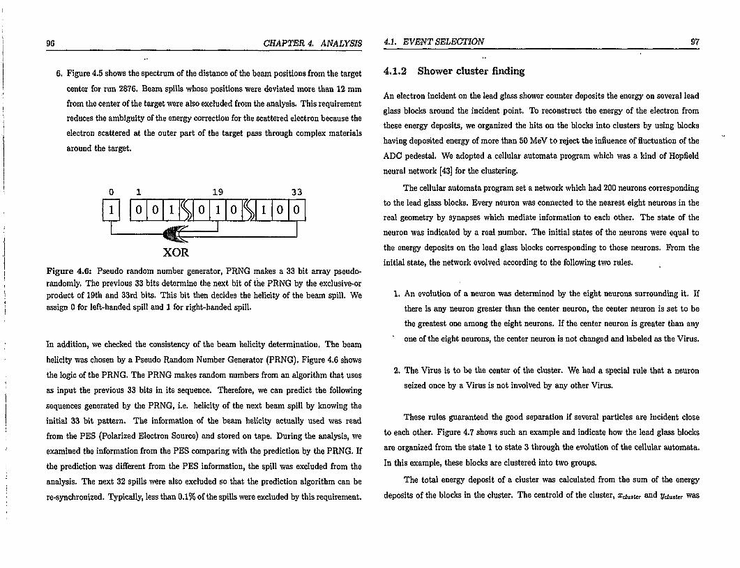
96 CHAPTER 4. ANALYSIS
6. Figure 4.5 shows the spectrum of the distance of the beam positions from the target center for run 2876. Beam spills whose positions were deviated more than 12 mm from the center of the target were also excluded from the analysis. This requirement reduces the ambiguity of the energy correction for the scattered electron because the electron scattered at the outer part of the target pass through complex materials around the target.
0 1 19 33
1 0 0 1 \ 0 1 0 \ 1 0 0
^ L _ 1
XOR Figure 4.6: Pseudo random number generator, PRNG makes a 33 bit array pseudo-randomly. The previous 33 bits determine the next bit of the PRNG by the exclusive-or product of 19th and 33rd bits. This bit then decides the helicity of the beam spill. We assign 0 for left-handed spill and 1 for right-handed spill.
In addition, we checked the consistency of the beam helicity determination. The beam helicity was chosen by a Pseudo Random Number Generator (PRNG). Figure 4.6 shows the logic of the PRNG. The PRNG makes random numbers from an algorithm that uses as input the previous 33 bits in its sequence. Therefore, we can predict the following sequences generated by the PRNG, i.e. helicity of the next beam spill by knowing the initial 33 bit pattern. The information of the beam helicity actually used was read from the PES (Polarized Electron Source) and stored on tape. During the analysis, we examined the information from the PES comparing with the prediction by the PRNG. If the prediction was different from the PES information, the spill was excluded from the analysis. The next 32 spills were also excluded so that the prediction algorithm can be re-synchronized. Typically, less than 0.1% of the spills were excluded by this requirement.
4.1. EVENT SELECTION 97
4.1.2 Shower cluster finding
An electron incident on the lead glass shower counter deposits the energy on several lead glass blocks around the incident point. To reconstruct the energy of the electron from these energy deposits, we organized the hits on the blocks into clusters by using blocks having deposited energy of more than 50 MeV to reject the influence of fluctuation of the ADC pedestal. We adopted a cellular automata program which was a kind of Hopfield neural network [43] for the clustering.
The cellular automata program set a network which had 200 neurons corresponding to the lead glass blocks. Every neuron was connected to the nearest eight neurons in the real geometry by synapses which mediate information to each other. The state of the neuron was indicated by a real number. The initial states of the neurons were equal to the energy deposits on the lead glass blocks corresponding to these neurons. From the initial state, the network evolved according to the following two rules.
1. An evolution of a neuron was determined by the eight neurons surrounding it. If there is any neuron greater than the center neuron, the center neuron is set to be the greatest one among the eight neurons. If the center neuron is greater than any one of the eight neurons, the center neuron is not changed and labeled as the Virus.
2. The Virus is to be the center of the cluster. We had a special rule that a neuron seized once by a Virus is not involved by any other Virus.
These rules guaranteed the good separation if several particles are incident close to each other. Figure 4.7 shows such an example and indicate how the lead glass blocks are organized from the state 1 to state 3 through the evolution of the cellular automata. In this example, these blocks are clustered into two groups.
The total energy deposit of a cluster was calculated from the sum of the energy
deposits of the blocks in the cluster. The centroid of the cluster, xa^ur and ydutur was

98 CHAPTER 4. ANALYSIS
0.2 3.0 1.0 0.2
0.3 0.2 0.4 W 2.0 0.2
2.0 P 1.0 0.4
0.2 0.6 0.3 0.2
&6 &0
W
&0 &a
3.0
I m&
1.0
H 2 -0 wlvlw ——
&12.0 m M m
8.0
4mr>
7.0 •
statel state2 state3 Figure 4.7: An evolution of cellular automata is shown in three steps, (a) The initial state. The states of the neurons are set to be equal to the energy deposit of the lead glass blocks. Neurons with no number mean that the energy deposit of the block is lower than the threshold, 50 MeV. Two cells filled by different gray colors are Viruses with the highest energy deposit in the surrounding blocks, (b) The next state. The neurons hatched by the light and dark gray colors are seized by these Viruses, (c) The final state. In this case, neurons are clustered into two groups. We notice that several cells seized by the 7.0 Virus were not seized by the 8.0 Virus in the evolution from (2) to (3) due to the second rules.
determined by,
E «*(»)« x{y)cXu,Ur = i = L g - (4.5)
E* « = 1
where i stands for the associated blocks, Ei is the energy deposit of the z-th block, a;,- and yi are the x and y position of the center of the i-th block. From a study for the matching between the reconstructed track and the cluster centroid, the spatial resolution was obtained to be about 10 mm [47]. Figure 4.10 and 4.11 show the spectra of the distances in x and y of the centroid of the shower cluster from the position of the reconstructed track for the 4.5° and 7° spectrometers. We notice that this spatial resolution includes the resolutions from the shower cluster centroid and the tracking position.
4.1. EVENT SELECTION
4.1.3 Track finding
The tracking was performed by using information from the Cerenkov counters, the hodo-scopes, and the shower counter. The information from these detectors were stored in a data format for the tracking routine. Every detector was virtually treated as a wire chamber in the tracking routine for convenience. The leading information contained in this data is
1. Three dimensional position specifying the wire location,
2. Vector parallel to the wire direction,
3. Spatial resolution of wires,
4. Timing of signals corrected by time of flight and propagation delay at the reference point (the surface of the shower counter),
5. Timing resolution.
In the case of hodoscopes, the line of the central axis of the finger is taken as the location and the vector of the wire. The spatial resolution was set to 1/VT2 of the finger width which was calculated from the square distribution. Table 4.1 shows the time resolution for each plane.
Because the Cerenkov counter covers all of the acceptance of the spectrometer, it was treated as a wire with a spatial resolution of 100 m. The time resolution of the counter was set to 1 ns.
A cluster of the shower cluster was interpreted as the hits of two wires along x and y axes whose intersection was at the center of the cluster. The position on the z coordinate was set to be zero at the surface of the shower counter. From a study for the matching in time between the shower cluster and the reconstructed track, the time resolution of the shower cluster was measured to be less than 1.0 ns [48]. Therefore, the spatial and time resolutions were set to 10 mm and 1.0 ns respectively.
100 CHAPTER 4. ANALYSIS
Plane 4.5° spectrometer (ns) 7° spectrometer (ns) 1 1.4 1.3 2 1.1 1.1 3 1.1 1.1 4 1.4 1.0 5 1.1 0.9 6 1.1 1.0 7 1.4 1.2
Table 4.1: Time resolution for hodoscope fingers in ns: the time resolution for every finger in a hodoscope plane was assumed to be identical.
For the track reconstruction, we first search hits in the time window of 15 ns in which we have the most hits. These hits were fitted for the reconstruction of the first track. Any hit deviated from the fit in either time or space, was removed from the fitting. If the number of the remaining hits was greater than those in any track classification shown in Table 4.2, the track was accepted. The fitting procedure was repeated until all tracks was reconstructed.
Glass Cerenkov Hodoscope Shower 1 1 4 1 2 1 4 0 3 0 4 1 4 0 6 0
Table 4.2: Track classification according to the minimum number of hits on each detector.
Figures 4.8 and 4.9 show the distance between the extrapolated point on the target and the center of the target where the extrapolation back on the target was performed by using the reverse matrix of the spectrometer magnet. We required that a track was reconstructed within 10 mm from the center of the target to be included in the analysis.
4.1. EVENT SELECTION 101
Figure 4.8: Track extrapolated position at target to the center of the target in the 4.5° spectrometer.
xto 4
30
25 •
;20
* 1 6
]- ft ; J
• i • i 1—1—0
•30
Figure 4.9: Track extrapolated position at the target to the center of the target in the 7° spectrometer.
Figure 4.10: Matching of tracks and clusters for the 4.5° spectrometer: The upper figure shows the matching in x, and lower figure shows the matching in y.
Figure 4.11: Matching of tracks and clusters for the 7° spectrometer: the upper figure shows the matching in x, and lower figure shows the matching in y.

102 CHAPTER 4. ANALYSIS
Figure 4.10 and 4.11 show the difference in x and y between the extrapolated position of the tracks on the shower counter and the center of the the shower cluster. We required that tracks and clusters have to be within 40 mm in both x and y, and 10 ns in time.
Tracking efficiency
Tracking efficiency does not affect the cross section asymmetry providing it is identical for the beam spills of both electron helicities. Of course, it would be a serious problem if the efficiency is different for the beam helicity because it may give a false asymmetry.
We examined the tracking efficiency by using the shower cluster. The fraction when the reconstructed track was properly associating to a shower cluster was defined to be the tracking efficiency.
We first have to remove any cluster produced by noise or gamma from the cluster sample because these contamination improperly decrease the tracking efficiency in this definition. To improve the purity of the cluster sample, we required the following,
1. No edge cluster. The cluster on the edge is unreliable because a part of the energy may leak to the outside of the shower counter.
2. Cluster energy greater than 8 GeV. The junk cluster was expected to be distributed
on such low energy region.
3. Both Cerenkov had a hit (low threshold)
4. Neural network response more than 0.9.
We adopted only electron clusters as the sample because we were able to require the Cerenkov hits and the neural network response and these requirements should purify the sample.
For the cluster sample, we examined matching with the tracks which was reconstructed by the regular tracking algorithm mentioned previously. We required that the
4.1. EVENT SELECTION 103
track is reconstructed within 40 mm in x and y, and 10 ns in time. These requirements were the same for those for the 'good track' in the usual analysis.
The tracking efficiencies were calculated separately for the beam helicity, +1 and - 1 and the spectrometers. Table 4.3 shows the results for run 1334. The tracking efficiencies had no significant difference for the beam helicities and produced no false-asymmetry.
Spectrometer 4.5° 7° helicity - 1 helicity +1
93.5 ±0.3 93.4 ±0.3
98.2 ±0.5 98.0 ±0.5
Table 4.3: Tracking efficiency
4.1.4 Electron identification
It is important to reject any hadron track from the analysis to obtain the cross section asymmetry because the cross section is defined by the number of scattered electrons. In principle, we can separate electron and hadron(pion) tracks by using (1) the Cerenkov counter and (2) the E/P ratio.
Cerenkov ADC
Basically, the long and short Cerenkov counters generate no signal for pions with the momentum less than 9 GeV/c and 13 GeV/c respectively. We can then reject the low momentum pion using the requirement for coincidence of the two Cerenkov counters.
Figures 4.12 to 4.15 show the ADC spectra of the Cerenkov counters. We required that the track fired the coincidence signal of the Cerenkov counters and the shower counter(main trigger) and the Cerenkov ADC value to be more than 40 for the track to be electron.
The detection efficiencies for electrons and the pion contaminations were estimated for the Cerenkov counters. For both of electron and pion samples, we required that the

104 CHAPTER 4. ANALYSIS
ADCnlut
Figure 4.12: ADC spectra of Cerenkov counter 1 for the 4.5° spectrometer. The solid line shows the ADC spectrum of Cerenkov counter 1 for electrons identified by the neural network response of the shower counter and the E/P ratio. The dashed line shows the spectrum for pions defined by the requirements for the neural network and E/p ratio opposite to those for electrons.
Figure 4.13: ADC spectra of Cerenkov counter 2 for the 4.5° spectrometer. The spectra are shown with the same convention as Figure 4.12.
4.1. EVENT SELECTION 105
ADCv«lu« ADCvilue
Figure 4.14: ADC spectra of Cerenkov counter 1 for the 7° spectrometer. The spectra are shown with the same convention as Figure 4.12.
Figure 4.15: ADC spectrum of Cerenkov counter 2 for the 7° spectrometer. The spectra are shown with the same convention as Figure 4.12.
track is 'good track' which has a good association to the target and the shower cluster. We rejected tracks associated to the edge of the shower counter because the shower cluster on the edge was less reliable. From the sample of the good track, the electron and pion sample was defined by E/P ratio and the neural network response which will be mentioned in Section 4.1.4. The requirements for the electron and pion samples are summarized;
1. electron,
(a) E/P ratio between 0.8 and 1.2,
(b) The neural network response more than 0.9,
2. pion ,
(a) E/P ratio less than 0.8,
(b) The neural network response less than 0.0.
The Cerenkov spectra are shown for these two samples. The efficiency for electron ID
were calculated from the fraction of electron tracks which had the Cerenkov ADC greater

106 CHAPTER 4. ANALYSIS
than 40. The pion contamination was calculated from the ratio of the pion sample to the electron sample with ADC value of more than 40. Table 4.4 shows the efficiency for electron ID and the pion contamination for the four Cerenkov counters. The good efficiencies of more than 95% were obtained for all Cerenkov counters.
4.5° CI 4.5° C2 7° CI 7°C2 Efficiency %
pion contamination % 99.1 ±0.0 14.6 ±0.1
97.7 ±0.0 7.0 ±0.1
97.6 ±0.1 12.9 ± 0.1
95.2 ±0.1 5.1 ±0.2
Table 4.4: Efficiency for electron ID and pion contamination of the requirement for the Cerenkov counters.
E/P ratio
E/P is a ratio of the energy measured by the shower counter to that obtained from the tracking. Since the mass of the electron is negligible, it has become custom in this analysis to label the tracking energy as "momentum" and the shower counter energy as "energy". The momentum was calculated from the tracking data using magnetic reverse matrix element, and the energy was extracted from the total energy deposited in the shower cluster.
Figure 4.16 and 4.17 shows the E/P ratios for the 4.5° and 7° spectrometers where we plotted only the "non-edge" sample given in Figure 3.34. The solid and dashed lines show the spectra for the electron and pion sample defined by using the hits from the Cerenkov counters and the neural network response of the shower counter. We accepted tracks with E/P of between 0.8 and 1.2 as electron tracks.
The efficiency for electron ID and the pion contamination were calculated using a electron sample and a pion sample which were defined by ADC value of the Cerenkov counters and the neural network response. We required for both of the electron and pion sample to be a 'good track' with a good association to the target and the shower cluster. The electron and pion samples were classified as follows:
4.1. EVENT SELECTION 107
02 M <.< OJ
Figure 4.16: E/P on 4.5° spectrometer: The solid line shows the E/P spectrum for electron defined by the Cerenkov counters and the response of the neural network. The dashed line is the E/P spectrum for pions excluded by Cerenkov counters and neural network.
Figure 4.17: E/P on 7° spectrometer with the same convention as figure 4.16.

108 CHAPTER 4. ANALYSIS
1. electron,
(a) Both Cerenkov ADC greater than 40,
(b) Neural network response more than 0.9,
2. pion,
(a) Both Cerenkov ADC less than 40,
(b) Neural network response less than 0.0.
The efficiency for electron ID and the pion contamination were calculated using the two samples. The efficiency for electron ID was the fraction of the electron sample in the region of E/P between 0.8 and 1.2. The pion contamination was the ratio of the pion sample to the electron sample in the region of E/P between 0.8 and 1.2. Table 4.5 shows the efficiency for electron ID and the pion contamination. This E/P cut did the effective pion rejection keeping the good efficiency for electron ID.
Spectrometer 4.5° 7° Efficiency %
Pion contamination % 94.4 ±0.1 0.4 ± 0.0
95.5 ±0.1 1.1 ± 0.0
Table 4.5: The efficiency for electron ID and the pion contamination of the requirement for the E/P ratio.
neural network
We also used a neural network algorithm to identify the type of particle incident onto the shower counter. The main difference in shower response between electrons and pions is the total of the energy deposit. Generally, a pion has a lower momentum than an electron because the pion comes from the fragmentation of a nucleon. In addition, a hadron will lose only a part of its energy in the shower counter. Therefore, the energy deposited by a pion is distributed mostly below 5 GeV with a 29GeV electron beam.
4.1. EVENT SELECTION 109
•i • " - i i f • • • £ • • • ' j j » ' • • ' j i ' • • '3!, Total tmrjy of» bkxki (G«V)
Figure 4.18: Total energy deposited in the nine blocks which are the central block of a cluster and eight blocks surrounding the central block. The upper and lower figures show the spectra for electron and pion samples. These electron and pion samples were defined by the ADC value of the Cerenkov counters and the E/P ratio.
, V • I ' J • - - ' • • • • ' • • • • i . . . • r ^ p . • 0 ( U O J OJ 0.« OS 0.6 0.7 0.8 0.9 ]
ES/(iumEl)
Figure 4.19s The ratio of the energy deposited in the central block of a cluster to the total energy deposited in the nine blocks defined in Figure 4.18 is plotted. The spectra are shown with the same conventions with Figure 4.18.
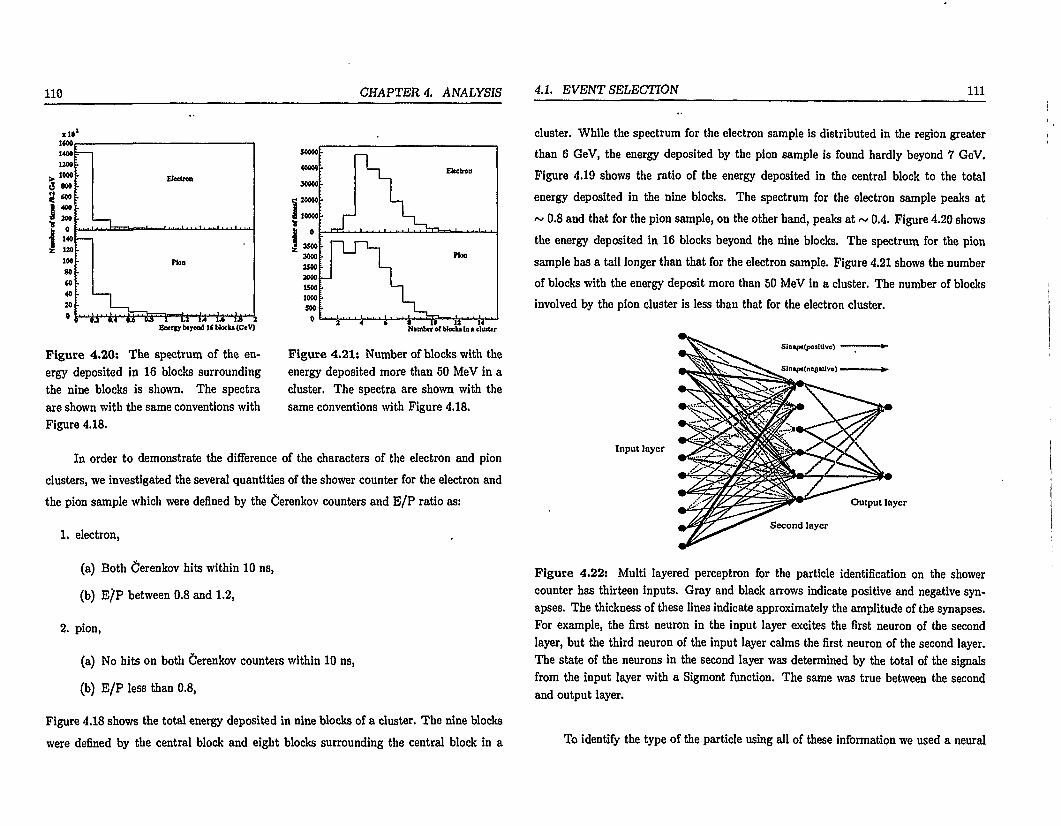
110 CHAPTER 4. ANALYSIS
1400 1200
. , 1000 Electron (J 800 -3 coo 8 4 0 . £ 200
;
1 140 • t t , !—,—,_«_, - • • • . . . i . . . t . . . i . . . i . . .
1 140 Z 120
100 Plon 80 «0 40 . 20 ft L...b^ 20 ft
r"« J M l i w " r~_u "u " W "W " 1 Energy beyond 1( bloclu (GtV)
Figure 4.20: The spectrum of the energy deposited in 16 blocks surrounding the nine blocks is shown. The spectra are shown with the same conventions with Figure 4.18.
50000 ._, 40004 • Electron
30000 -2O0M • 10000
0
3500
LxL...-10000
0
3500 3000 PlOD
1500 MOO 1500 1000 500
0 • . . » . . . i . . . i . . . i . . < - I - I . • . . . i . . 500
0 2 4 i a i* u 14 Number of bloclu la a cluster
Figure 4.21: Number of blocks with the energy deposited more than 50 MeV in a cluster. The spectra are shown with the same conventions with Figure 4.18.
In order to demonstrate the difference of the characters of the electron and pion clusters, we investigated the several quantities of the shower counter for the electron and the pion sample which were defined by the Cerenkov counters and E/P ratio as:
1. electron,
(a) Both Cerenkov hits within 10 ns,
(b) E/P between 0.8 and 1.2,
2. pion,
(a) No hits on both Cerenkov counters within 10 ns,
(b) E/P less than 0.8,
Figure 4.18 shows the total energy deposited in nine blocks of a cluster. The nine blocks
were defined by the central block and eight blocks surrounding the central block in a
4.1. EVENT SELECTION 111
cluster. While the spectrum for the electron sample is distributed in the region greater than 6 GeV, the energy deposited by the pion sample is found hardly beyond 7 GeV. Figure 4.19 shows the ratio of the energy deposited in the central block to the total energy deposited in the nine blocks. The spectrum for the electron sample peaks at ~ 0.8 and that for the pion sample, on the other hand, peaks at ~ 0.4. Figure 4.20 shows the energy deposited in 16 blocks beyond the nine blocks. The spectrum for the pion sample has a tail longer than that for the electron sample. Figure 4.21 shows the number of blocks with the energy deposit more than 50 MeV in a cluster. The number of blocks involved by the plon cluster is less than that for the electron cluster.
Figure 4.22: Multi layered perceptron for the particle identification on the shower counter has thirteen inputs. Gray and black arrows indicate positive and negative synapses. The thickness of these lines indicate approximately the amplitude of the synapses. For example, the first neuron in the input layer excites the first neuron of the second layer, but the third neuron of the input layer calms the first neuron of the second layer. The state of the neurons in the second layer was determined by the total of the signals from the input layer with a Sigmont function. The same was true between the second and output layer.
To identify the type of the particle using all of these information we used a neural
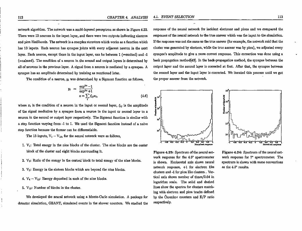
112 CHAPTER 4. ANALYSIS
network algorithm. The network was a multi-layered perceptron as shown in Figure 4.22. There were 13 neurons in the input layer, and there were two outputs indicating electron and pion likelihoods. The network is a complex structure which works as a function which has 13 inputs. Each neuron has synapse joints with every adjacent neuron in the next layer. Each neuron, except those in the input layer, can be between 1 (=excited) and -1 (=calmed). The condition of a neuron in the second and output layers is determined by all of neurons in the previous layer. A signal from a neuron is mediated by a synapse. A synapse has an amplitude determined by training as mentioned later.
The condition of a neuron, yt was determined by a Sigmont function as follows,
_ exp*tt - 1 Vi ~ exp*°+l
a = £&*.-> (4.6) >
where Xi is the condition of a neuron in the input or second layer, £y is the amplitude of the signal mediation by a synapse from a neuron in the input or second layer to a neuron in the second or output layer respectively. The Sigmont function is similar with a step function varying from -1 to 1. We used the Sigmont function instead of a naive step function because the former can be differentiable.
The 13 inputs, Vi — Vj3, for the neural network were as follows,
1. Vi: Total energy in the nine blocks of the cluster. The nine blocks are the center block of the cluster and eight blocks surrounding it.
2. V2: Ratio of the energy in the central block to total energy of the nine blocks.
3. V3: Energy in the sixteen blocks which are beyond the nine blocks.
4. V4 - VW Energy deposited in each of the nine blocks.
5. V13: Number of blocks in the cluster.
We developed the neural network using a Monte-Carlo simulation. A package for
detector simulation, GEANT, simulated events in the shower counters. We studied the
4.1. EVENT SELECTION 113
response of the neural network for incident electrons and pions and we compared the responses of the neural network to the true answer which was the input to the simulation. If the response was not the same as the true answer (for example, the network said that the cluster was generated by electron, while the true answer was by pion), we adjusted every synapse's amplitude to give a more correct response. This correction was done using a back propagation method[43]. In the back-propagation method, the synapse between the output layer and the second layer is corrected at first. After that, the synapse between the second layer and the input layer is corrected. We iterated this process until we got the proper answer from the network.
Ncur«l Mt respoosv
Figure 4.23: Spectrum of the neural network response for the 4.5° spectrometer is shown. Horizontal axis shows neural network response, +1 for electron like clusters and -1 for pion like clusters. Vertical axis shows number of times/0.04 in logarithm scale. The solid and dashed lines show the spectra for clusters matching with electron and pion tracks defined by the Cerenkov counters and E/P ratio respectively.
Figure 4.24: Spectrum of the neural network response for 7° spectrometer: The spectrum is shown with same conventions as the 4.5° results.

114 CHAPTER 4. ANALYSIS
Figure 4.23 and 4.24 show the neural network response for run 1334. The horizontal axis shows the response which is 1 for electron clusters and -1 for pion clusters. The solid and dashed lines show the responses for the electron and pion samples respectively defined by the Cerenkov counters and the E/P ratio. We required that the neural network response had to be more than 0.9 to identify a particle as an electron.
The efficiency for electron ID and the pion contamination were extracted by a calculation similar to that for the ADC of the Cerenkov counters or the E/P ratio. The electron and pion samples were defined by
1. electron,
(a) Both Cerenkov ADC more the 40,
(b) E/P ratio between 0.8 and 1.2,
2. pion,
(a) Both Cerenkov ADC less than 40,
(b) E/P ratio less than 0.8.
Table 4.6 shows the efficiency for electron ID and the pion contamination calculated from these electron and pion samples. The results indicate the higher efficiency and the lower pion contamination comparing to a conventional method for the particle identification resulting ~90% of efficiency for electron ID and ~10% of pion contamination[43].
4.5° 7° Efficiency %
Pion contamination % 98.1 ± 0.0 0.3 ± 0.0
98.8 ±0.0 0.8 ±0.0
Table 4.6: Efficiency for electron ID and pion contamination for neural network response
4.1. EVENT SELECTION 115
The electron sample
Finally, the requirements for the electron sample are summarized to be
1. The main-trigger fired,
2. The ADC outputs from both Cerenkov counters were more than 40,
3. The track extrapolated back to the target within 10mm in x,
4. Track and Cluster agreed with each other by less than 40 mm in x and y and less' than 10 ns in time,
5. 0.8 < E/P < 1.2,
6. neural network response was more than 0.9,
* "_.
"tr* £ $ 8 . a 1 £ 'bi
-:
. ..;;sii ! = = •
-^
F "
f
F "
f ^ ^ i . i . i i i
vx' BJorkcax
Figure 4.25: Data profile on x—Q2 plane from run 1334 for the 4.5° spectrometer. The x and y axes show Bjorken x in logarithmic scale and Q 2 in linear scale respectively. The box area is proportional to the number of counts in each bin in logarithmic scale.
BJorlceax
Figure 4.26: Data profile on x - Q2
plane from run 1334 for the 7° spectrometer with the same convention as Figure 4.25.

116 CHAPTER 4. ANALYSIS
We obtained electron data scattered inelastically from the deuteron target over a wide kinematical region as shown in Figure (4.25) and (4.26). The kinematics for the electron was calculated using the momentum evaluated from the tracking with the reverse matrix of the spectrometer magnets and the scattered angle from the beam axis. We excluded counts outside the deep-inelastic region where the momentum transfer was less than 1.0(GeV/c)2 where the scaling is not a good approximation for the structure function due to the large strong coupling constant. We also excluded data in the resonance region where the effective mass of the final hadron system was less than 2.0GeV/c2. The e-N scattering has A resonances in the region where the cross section does not indicate the proper information of the nucleon structure.
When satisfied, these two kinematical conditions retained enough statistics to give the cross section asymmetry in the region from 0.029 to 0.8 in Bjorken x and from 1.0(GeV/c)2 to 12.0(<7eV/c)2 in Q2. The representative values of a; and Q2 for a bin was calculated from the averaged x and Q2 over the data which were included in the bin.
4.2 The cross section asymmetry
As the results of the analysis in the previous section, we obtained a clean electron sample from the measurement. The purpose of this section is a derivation of the cross section asymmetries A\\ and Ax- These cross section asymmetries are calculated from the number of scattered electrons off the polarized deuteron target.
If we assume that the beam is polarized 100% and the pure deuteron target is also longitudinally or transversely polarized 100%, a number of electrons detected by the spectrometer, Jv"N*"Wtt is expressed by,
jVttHWt) = <T«<-M»QK*-Wnp(t)NAin(t) (H = L, R), (4.7)
where the superscripts of the arrows for N, cr, and Q indicate the directions of the target and beam helicities, a is the cross section for the scattering, Q is a total beam flux, p(t) is the target density, N& is the Avogadro number, I is the length of the target, and ft(i)
4.2. THE CROSS SECTION ASYMMETRY 117
is the acceptance and the detection efficiency of the spectrometer. In principle, the p(i) and the Sl(t) may change during the experiment and then are functions of the time, t.
Using the number of electrons detected by the spectrometer and the total beam flux, the rate asymmetry is written by
_ N«*-n/QU<-n _ ;yt«-)t/Qt«-)t "<x> ~ 7Vt«->l/Qt(H; + 7Vt«-)t/Qt(«-)t ( 4 , 8 J
Although the target density and the acceptance and the detection efficiency of the spectrometer was varied during the experiment, influences due to the time fluctuation of these factors was negligible because the beam helicity was changed randomly spill by spill. Therefore, the factors of p(t)NAlil(t) were same for left- and right-handed spills and were canceled in the rate asymmetry. The rate asymmetry is then supposed to be same as the cross section asymmetry in the ideal case.
In the actual experiment, the beam polarization and the target polarization were less than 100% and the target contained many nucleons other than the deuteron. The beam and target polarization and the dilution factor which is the ratio of electrons scattered from the deuteron to those from all of the target materials relate the rate asymmetry to the cross section asymmetry to be
where pt, is the beam polarization, pt is the target polarization, and / is the dilution
factor. Equations (4.9) is the relation of the rate asymmetry and the cross section asym
metry accounting only the leading corrections. Actually, the other corrections smaller than these leading corrections are also important to the high precision measurement for the spin structure function. To do that, we measure the rate asymmetry not only for the electron, but also for the positron defined to be
,It-L) ~ m*iQi&-»+N$-*/Q#-* ( 0 )
where Ajj^j is the rate asymmetry for the electron and positron, Nlfg~M is the number
of electrons or positrons detected by the spectrometer, Ql§~^ is the total of the beam

118 CHAPTER 4. ANALYSIS
current. The rate asymmetry for the positron was investigated reversing the polarity of
the spectrometer magnet. In the following subsections, we will discuss about the procedure to extract the cross
section asymmetry from the rate asymmetry measured directly in the experiment.
4.2.1 The dead time correction
The dead time correction is defined by the ratio between the true trigger rate and the measured trigger rate. The dead time effect basically depends on the trigger rate. Consequently, it may affect the rate asymmetry if the trigger rates for left- and right-handed spills had a large difference.
The rate asymmetry corrected by the dead time effect is expressed as,
where CL,R is the dead time coefficient for the electron (positron) rate obtained by the left- or right-handed spill.
We calculated the dead time coefficient for a given run;
] £ < m l > xP(n,m)
2_,mm(m,4) x tm
m
where t m is the number of times there were m trigger(s) in a spill, n is the index to indicate the expected trigger rate, and P(rj,m) is the matrix element which is defined as the probability to detect m triggers if there are n real triggers. Because the number of triggers in a spill was limited by shower counter electronics to four or less, the measured trigger number could only go up four even if there were more triggers in a spill. The term of min(m, 4) was inserted instead of m due to this trigger logic.
The matrix element P(n, m) was calculated by a Monte Carlo simulation[49]. In the simulation, we assumed;
4.2. THE CROSS SECTION ASYMMETRY
1. Triggers distributed randomly in time,
2. Dead time between triggers was 32ns,
3. n and m were limited to 10.
The 10 x 10 unitary matrix elements are shown in Table 4.7.
measured trigger
true trigger measured trigger 1 2 3 4 5 6 7 8 9 10
1 1.000 0.028 0.002 2 0.972 0.086 0.007 3 0.913 0.155 0.019 0.003 4 0.838 0.235 0.049 0.008 0.002 5 0.745 0.321 0.088 0.022 0.006 0.002 6 0.627 0.371 0.147 0.049 0.013 7 0.532 0.407 0.206 0.083 8 0.422 0.415 0.249 9 0.323 0.405 10 0.249
Table 4.7: The probability matrix to the number of triggers detected by the spectrometer. The matrix elements are calculated under the assumptions dead time=32 ns, Spill length=2200 ns. A blank means the element is 0.
We did not assume symmetry between left- and right-handed spills for the dead time coefficient, i.e. the coefficients were calculated separately for each handedness.
The dead time correction for both spectrometers are shown in Figure 4.27 and 4.28. The dead time coefficient depends on the trigger rate, and that increased the trigger rates by several percents. The corrections for the left- and right-handed spills usually were similar, so the dead time correction was very small on the asymmetry. Figure 4.29 and 4.30 indicate the asymmetry of the dead time correction for left- and right-handed spills defined by,
Adc = CL — CR CL + CR'
(4.13)

120 CHAPTER 4. ANALYSIS
1.08
1.07 •
1.06 -/ 1.05 - V,
1.04 - / ' 1.03 : 1.02 - •''' 1.01
1.0
o.» 0
- • '.•*• 1.01
1.0
o.» 0
1.01
1.0
o.» 0 10 <U5 0l5 0.75 ! 1-25 1,5 1.75 2
Averaged trigger rate
Figure 4.27: Dead time correction as a function of the averaged trigger rate for the 4.5° spectrometer: the horizontal axis shows the averaged rate for main-or trigger. The vertical axis shows the dead time correction. Only the results for left handed spill are plotted.
70 •S2 ; <o I ?*>
40
30
20
10
Entries 19! Mean 0.I24E-O5 RMS 0300E-OJ
JL kw •0.15 -4.1 -4.05 • 0.05 0.1 0.15 xt(T 2
asymmetry
Figure 4.29: The left-right asymmetry on the dead time correction for the 4.5° spectrometer.
0.0 025 03 0.75 1.25 1.5 1.75 2 Averaged trigger rat.
Figure 4.28: Dead time correction for the 7° spectrometer. The data for the left handed spill are shown with the conventions same as Figure 4.27.
100
-
Entries 195 Mean -0.127E-04 RMS 0.156E-03
12
I" r z
-
40 -
20 -
0 • . . . . i n_ i-J. . . 0 -0.15 -0.1 -0.05 9 0 05 0.1 0.15 ,tfl;2
asymmetry
Figure 4.30: The left-right asymmetry on the dead time correction for the 7° spectrometer.
4.2. THE CROSS SECTION ASYMMETRY 121
The uncertainty of the dead time correction was estimated to be less than 1.0% of (1 - Ci,a) from the detail study of the simulation. Therefore, the uncertainty on the asymmetry from the dead time correction was negligible.
4.2.2 beam polarization
0.95
0.90
0.85
0.80
0.75
1 1 1 1 1 1 r E 143 Double Arm Mailer Polarization vs QE
n o • a M e a n
H+fk Systematic error ± 0.02
H » K j » » 4 J_
0.04 0.08 QE (%)
0.12 0.16
Figure 4.31: The electron polarization is plotted as a function of the quantum efficiency of the cathode of the polarized electron source. The electron polarization is measured by ESA M0ller polarimeter. The a shows the spread of the measurements and the OMean shows the mean of these measurements. A step function plotted by a solid line was obtained from the fit with the ouean and determined the beam polarization in the analysis.
The beam polarization was determined by ESA M0ller polarimeter as mentioned in Section 3. The results from the single arm polarimeter and the double arm polarimeter, and also the Linac polarimeter which is located at the end of the Linac, were in good agreement with each other[34].
Figure 4.31 shows the relation between the quantum efficiency of the electron cathode and the beam polarization measured by the ESA Miller polarimeter. The a shows the spread of the measurements and the ffjifeam is the mean of these measurements. From a

122 CHAPTER 4. ANALYSIS
step function obtained from a fit to the aMeant the beam polarization was determined for each run. The beam polarization was 84 - 86% during the experiment with the absolute uncertainty of 2%.
4.2.3 Target polarization
: "
\\ !"•• 1 i,»
: ; J.«i
: \ • '
\ , • • ! 1* 1 ;1 i Hi.
Ti-rr
,
r 1 . . . t . . i . 1 1 1 1 1 1 1 1 1 1 1 . . . I . . . I . . . 1400 1800 2200 2600 3000
run number
Figure 4.32: The horizontal axis shows run number, the vertical axis shows the ND3
target polarization. The sign of the polarization is plus for forward, minus for backward to the beam direction.
Target polarization was measured by the NMR signal obtained by the Q-meter module of the Liverpool type calibrated by that for the thermal equilibrium shown in Figure 3.17. The uncertainty of the target polarization was dominated by the statistical error of the NMR measurement for thermal equilibrium to be 4.0% relative to the polarization [50].
Figure 4.32 shows the target polarization during the experiment as a function of the run number. The negative polarization mean that the direction of the polarization is opposite to the beam direction. The target polarization was obtained up to 40% and the average was about 25%.
4.2. THE CROSS SECTION ASYMMETRY 123
0.2 03 J 0 0.4 0.5 Beam current (Iff eleclron/spUl)
Figure 4.33: The correction for the target polarization due to the beam heat effect. The horizontal axis shows the beam current in a unit of lO'O electron/spill. The vertical axis shows the correction in % defined by the difference of the corrected polarization from the measured polarization.

124 CHAPTER 4. ANALYSIS
The electron beam heated up the target center where the beam was rastered and the fringe part of the target was refrigerated by the circulated liquid helium directly. So, the target had a gradient of its temperature between the center and the fringe parts. Because the deuteron polarization depends on the temperature, the deuteron polarization is not uniform in the target cell due to the temperature gradient.
On the other hand, the NMR coil surrounded the larger volume of the target material than the volume which was actually on the beam line. So, the results from the NMR measurement averaged the gradient of the target polarization and gave a polarization higher than the polarization where the beam was rastered. The correction was estimated from the actual depolarization with varying the beam current [51]. The correction decreased the target polarization by 1.5% of that with a typical electron current. The correction factor for each run are plotted in Figure 4.33 as a function of the beam current. The correction factor is defined to be the difference between the uncorrected and corrected beam polarizations.
4.2.4 Dilution factor
The target contains not only polarized deuterons, but also unpolarized materials. The materials decrease the asymmetry in proportion to a factor called the dilution factor.
The dilution factor is the ratio between the number of electrons scattered from the deuterons in ND3 and that from all materials. Neglecting common factors like Avogadro number and Beam flux etc., the number of electrons scattered by a material is generally to be
N = ?j-(Np<jp + Nn<Tn)g, (4.14)
where p is the density of the material, I is the length of the material, A is the mass number of the nucleus, Np and N„ are the numbers of proton and neutron in the nucleus, crp and a„ are the cross sections for proton and neutron respectively, and g is the EMC effect coefficient for the nucleus. The EMC effect coefficient is the ratio of the cross section per nucleon between a heavier nucleus and a deuteron. The EMC effect coefficient was
4.2. THE CROSS SECTION ASYMMETRY 125
determined by a fit done by S. Rock and L. Stuart using the data of deep-inelastic scattering experiments[52][53].
We introduced the packing fraction p/ which is the percentage of the target cell occupied by ND3 beads. The number of electrons scattered from the ND3 is expressed using the packing fraction by,
N N D 3 = Psm-Ua-Pt { 3 ( ( 7 p + , B ) + {7<Tp + 8 a n ) g N } ( ( 4 1 5 )
where p^D3 is the density of ND3, 21 is the atomic mass number of ND3, lccu is the length of the target cell, and g^ is the EMC effect for nitrogen nuclei. Similarly, the number of electrons scattered from the deuteron is
ND = 21 3( c rp + an)- (4.16)
We assumed that the other parts of the target cell were filled by liquid helium. The
number of electrons scattered from the liquid helium is then expressed as,
' N H e = ftr.-lirP-P/)^ + 2 ( 7 n ) ) ( 4 1 7 )
where the pne is the density of the liquid helium.
There were also other materials in or around the target, for example the wall of the cell, the NMR coil etc. Accounting for all of these materials, the dilution factor, / was calculated as follows,
f = NND3 + NHe + ENcther,' ( 4 ' 1 8 )
where the £ Nothera represents the contributions from materials other than ammonia and helium.
We divide both of the numerator and the denominator by ap to simplify such that ap
and an are replaced by 1 and a„/ap respectively. In the actual calculation, we assumed the ratio of an/ap is equal to F2n/F2p which is calculable from the well measured F2&jFip. The Figures 4.34 and 4.35 show the dilution factor for the 4.5° and 7° spectrometers. The dilution factor was obtained to be 0.23 ~ 0.25 depending on x because of the variation of the cross sections and the EMC effect. The error of the dilution factor was calculated from the errors of the cross section, EMC effect, the packing fraction, density of materials.

126 CHAPTER 4. ANALYSIS
BJorkenx
Figure 4.34: Dilution factor on 4.5° spectrometer. The dilution factors are calculated from averaged a; and Q2 for each data point.
• • • • • • • • M M •••••••
BJotktnx
Figure 4.35: Dilution factor on 7° spectrometer. The dilution factors are calculated from averaged x and Q2 for each data point.
4.2.5 Nitrogen correction
Nucleons (nuclei) other than deuteron could either dilute the asymmetry, or contribute to the asymmetry because a small fraction of these nucleons (nuclei) is polarized. In addition, a contamination of NH3 gives an asymmetry of protons. We named the correction due to these polarized nucleons (nuclei) other than deuterons as nitrogen correction.
As mentioned in Section 3.4, we used 1 5 ND 3 as the target material. The nominal 1 4 N nucleus contaminated the target material by 2.0%. The contamination of proton, ie. NH3, was estimated to be 1.5%. These three kinds of nuclei and nucleon other than deuteron, 1 5 N, 1 4 N, and proton, were polarized in the target. These nitrogen and proton polarizations as a function of the deuteron polarization were measured as shown in Figure D.2 and D.l. We measured only the 1 5N polarization and assumed that the 1 4N polarization had the same magnitude and the sign opposite to that for the , 5 N.
Assuming the contamination by these nuclei and nucleon, the cross section asym-
4.2. THE GROSS SECTION ASYMMETRY 127
metry was corrected by the nitrogen correction as follows l ,
^ - J ? (Aft)' .]. M A , (4.19) , PdPdf
where the factor of v\ and v2 are the functions of the deuteron polarization and typically to be
vx ~ 0.98, (4.20)
u2 ~ 0.06, (4.21)
and Ah is the asymmetry for the proton measurement which we used the results from the E143 measurement using NH3 target for.
This correction depends on the deuteron polarization varied due to the experimental conditions and the correction was then applied for each run in the analysis.
4.2.6 Positron subtraction
The measured tracks are not only electrons which come from deep-inelastic scattering, but also from other processes, such as pair creation by gammas from neutral pion.
Taking an account of the processes other than deep-inelastic scattering, the cross section counting the electron, fft(+-M(t) j s expressed by,
^m=4rm + 4tm, (4.22) where the cross section counting the electron from the deep inelastic scattering,
and <7ja£ is the cross section counting the electron from the pair creation etc. We assumed that the cross section counting electrons from the back-ground pro
cesses for deep-inelastic scattering was charge symmetric. Under the assumption, this cross section was estimated from the measurement counting positrons using the reverse magnetic field because the positrons came only from the charge symmetric process. Therefore, the cross section counting the positron oJ^MCt) gives the cross section of the charge
1refer Appendix D for the detail of the derivation of the formula.

128 CHAPTER 4. ANALYSIS
symmetric process as,
4itm = 4iHm- (4-23) The cross section for deep-inelastic scattering was extracted by subtracting the
cross section counting positrons from that counting electrons. We define the total cross sections, ae and ap, and cross section asymmetries, Ae and Ap, counting electrons and positrons by,
o* = o ^ + of^\ (4.24)
ffP = o-«HI + £ 7J«-)t ) (4,25)
fft(«-H _ a t«-) t 4x) = <$+•» +Jp-n ( 4 , 2 7 )
The cross section asymmetry for deep-inelastic scattering, Aftl, is described with these
electron and positron cross sections by, _ ( g t (HI- g t (H+). ( g t (<-) t . g t (<-) t )
A\U) ~ ( f f t ( H * _ a t ( H ; ) + ( a t (H t_ a t (H t )
- 4(J.)^F-4(X)^?- (4-28) ae
The factor is the correction for the dilution for the cross section asymmetry due oe-aP to the contamination of the charge symmetric process. The second term in Equation (4.28) is the correction due to the asymmetry which the charge symmetric process has. Figures 4.36 to 4.43 show these factors.
In the actual calculation, we used the electron and positron asymmetry obtained from the Equation 4.19 for the ideal A» and Av in the Equations (4.26) and (4.27). We used also the ratio of the counting rates defined to be
for the ideal ratio of the ae/(ae - ap). This is true for the ratio of the crp/{ae — ap). It is allowed if the temporal fluctuation of the target density and the acceptance and efficiency
4.2. THE CROSS SECTION ASYMMETRY 129
_ f l L M
1.075
• « 1.075
1.05 • •
1.05
I.0Z5 • • 1.025
1 1 1 1
0.975 : 0*75
OX : 0.95
0.915 • 0*15
0.9 10'
Figure 4.36: The correction for the dilution due to the contamination of electrons from processes other than deep-inelastic scattering on 4.5° spectrometer for A\\.
Figure 4.37: The correction for the dilution due to the contamination of electrons from processes other than deep inelastic scattering on 7° spectrometer for A\\.
Figure 4.38: The correction for the dilution due to the contamination of electrons from processes other than deep-inelastic scattering on 4.5° spectrometer for A±.
Figure 4.39: The correction for the dilution due to the contamination of electrons from processes other than deep-inelastic scattering on 7° spectrometer for Ax.

130 CHAPTER 4. ANALYSIS
Figure 4.40: The correction due to the asymmetry of the charge symmetric process on 4.5° spectrometer for A\\.
Figure 4.41: The correction due to the asymmetry of the charge symmetric process on 7° spectrometer for A\\.
Figure 4.42: The correction due to the asymmetry of the charge symmetric process on 4.5° spectrometer for Aj_.
Figure 4.43: The correction due to the asymmetry of the charge symmetric process on 7° spectrometer for A±.
4.2. THE CROSS SECTION ASYMMETRY 131
of spectrometers were averaged and there was no bias for the electron and positron data and the assumption was guaranteed because we changed the magnet setting several times during the experiment.
4.2.7 Radiative correction
The cross section for deep-inelastic scattering is dominated by the one photon exchange process as shown in the Feynman diagram in Figure 2.1. However, the actual processes of the deep-inelastic scattering contain not only the naive one photon exchange process, but also other processes, for example two photon exchange processes, vacuum polarization, internal-bremsstrahlung etc. In addition, the energy of the scattered electron is varied by the interaction with the external field. To extract the cross section asymmetry for the one photon exchange process from the measured cross section asymmetry, we should estimate the radiative correction.
The radiative correction is categorized into internal and external radiative corrections. The internal radiative correction is due to processes involving self interaction like vertex correction or real photon emission. The external radiative correction is due to interactions with external fields. Leading diagrams accounting in the radiative correction, are shown in Figure 4.44.
The internal radiative correction was calculated based on the method by N.Kukhto and N.Shmeiko [54]. In the radiative correction, contributions from the various higher order diagrams and radiative processes were accounted as follows:
1. Electron vertex correction,
2. Vacuum polarization,
3. Two photon exchange,
4. Elastic radiative process,
5. Quasi-elastic radiative process,

132 CHAPTER 4. ANALYSIS
RADIATIVE CORRECTIONS
Proton. (a) Lowest Order Graph (b) Internal Bremsstrahlung (s-peak)
Es ^ , c s En
(c) Internal Bremsstrahlung (p-peak) (d) External Bremsstrahlung (s-peak)
(e) External Bremsstrahlung (p-peak) (f) Vertex Correction
(g) Vacuum Polarization 12-93 7585A12
Figure 4.44: Leading diagrams accounting the in radiative correction
4.2. THE CROSS SECTION ASYMMETRY 133
6. Inelastic radiative process.
The proton and neutron form factors for elastic- and quasi-elastic processes were taken from References [55] and [56]. The deuteron form factor for elastic- and quasi-elastic radiative processes was extracted from a fit done by L.M.Stuart [57]. The unpolarized nucleon structure function for inelastic radiative process was taken from References [59] and [60].
0.01
0.005
•O.005-
-0J)1-
•0.015 •
•0.02
0.01
X Bjorkcn
Figure 4.45: Radiative correction on 4.5 ° for An
X Bjorken
Figure 4.46: Radiative correction on 4.5° for A±
The external radiative correction was calculated by Stuart [57] with the formula of
*«i(t., h) = J I(E0, E, tb)<rint(E, E')I(E', E'F, QdEdE', (4.30)
where E0 is the initial energy of electron, E'F is the energy of the final state electron, and I(E, E', t) is the probability that the energy E becomes to E' after passing through a material of depth t. Then, Equation (4.30) means a cross section that final scattered electron has energy E'F for given materials.
The external radiative correction was calculated assuming a target model estimated by T. Liu [51] accounting only the external bremsstrahlung.
Figure 4.45 , 4.46, 4.47, and 4.48. show the evaluated radiative correction for A\\ and Ax. of the 4.5° and 7° spectrometers. The radiative correction, #Cj|,i, is the difference

134 CHAPTER 4. ANALYSIS
1 0.01 r
;0.005-i u
3 o -
•0.005-
•0.01 •
•0.015 •
•OJ02- 10 XBJorken
8 ° ' 0 1
|0 .008
80.006
l o .004 |o .002
0
•0.002
•0.004
•0.006
•0.008
•O.01
-Jim o
i 10 XBJorken
Figure 4.47: Radiative correction on 7° for Au
Figure 4.48: Radiative correction on 7° for A±
of the cross section asymmetry defined by the one photon exchange process ( Born cross section ), A\\,x, and that defined by the measured cross section including any radiative and higher order interactions, /ijfj .
4i.j.=4:'i + i* ciu- (4.31)
The radiative correction for A\\ decrease the asymmetry in low-x region by less than 0.01. On the other hand, the radiative correction for A± is consistent with zero but the large uncertainty.
We defined the radiative correction for the cross section asymmetry in the additional form as shown in Equation (4.31). The reason why we did not introduce the multiplicative form was the definition is too sensitive to the statistical fluctuation on where the asymmetry, .djf'i was very small. In principle, the radiative correction due to the background from the elastic and quasi-elastic scattering etc. should be defined to be a multiplicative form and it corrects not only the central point of the data, but also the magnitude of the statistical error. Therefore, We prepared another correction factor for the statistical error. The statistical error was corrected by the factor to be
*n = <f7*qf. (4.32)
4.2. THE CROSS SECTION ASYMMETRY 135
Figure 4.49: Radiative correction for statistical error of A\\ in the 4.5° spectrometer
Figure 4.50: Radiative correction for statistical error of A\\ in the 7° spectrometer
where 6\\ is the statistical error radiatively corrected, 6ff' is the statistical error for the asymmetry before the radiative correction, and RCtf is the correction factor. The factor for A\\ on both spectrometers was calculated as shown in Figures 4.49 and 4.50.
4.2.8 Results
The corrections from the dead time, the beam polarization, the target polarization, the dilution factor, and the nitrogen polarization are the factors which depend strongly on the experimental conditions. We then applied these corrections for each run data. Results from many runs were summarized on the corrected asymmetry separately for the target configuration (longitudinal or transverse), the spectrometer (4.5° or 7°), and the spectrometer magnet setting (electron or positron mode) as follows,
<A(x)^>= ?^wrx)2
(4.33)

136 CHAPTER 4. ANALYSIS
Figure 4.51: A\\ on 4.5° spectrometer Figure 4.52: Ax on 4.5° spectrometer
where < j4(a;)jj' > is the averaged asymmetry, (Aj(a;)jj^)' is the rate asymmetry corrected by the dead time effect, 5<(a;)^ is the statistical error of the cross section asymmetry for each run.
OSr
Figure 4.53: A\\ on 7° spectrometer Figure 4.54: As. on 7°. spectrometer
The cross section asymmetry for the deep-inelastic process was calculated by using
the Equation (4.28) with the averaged electron and positron asymmetry. Finally, we
4.2. THE CROSS SECTION ASYMMETRY 137
applied the radiative correction for the asymmetry. Figure 4.51, 4.52, 4.53, and 4.54 show the results of the cross section asymmetry for both spectrometers and both target configurations.
4.2.9 Study for the systematic effects on the asymmetry
We studied the systematic effects on the cross section asymmetry caused by the direction of the target polarization and the magnetic field on the target.
0.5 US 2 25 3 35 4 Chi square
Figure 4.55: The x 2 distribution of the difference of the J4|| taken with different target polarization direction in 4.5° spectrometer.
v 0 OS 1 IS 2 2.5 3 35 4 Chi square
Figure 4.56: The x 2 distribution of the difference of the A± taken with different target polarization direction in 4.5° spectrometer.
The target is polarized by the DNP method with a strong magnetic field and a microwave relaxation technique as mentioned in Section 3. The combination of the direction of the magnetic field and the wave length of the microwave determines the direction of the target polarization. The backward and forward polarization is then possible with the same magnetic field.
We calculated the asymmetry separately for runs which were taken with the positive
and negative polarization and magnetic field respectively. Then, we took the difference

138 CHAPTER 4. ANALYSIS
V I 8-
6
4
2
0 ' 3 - i rr 05 15 25 3 35 4
CM square
Figure 4.57: The x 2 distribution of the difference of the A\\ taken with different target polarization direction in 7° spectrometer.
3 35 4 CM square
Figure 4.58: The x 2 distribution of the difference of the Ax taken with different target polarization direction in 7° spectrometer.
of these two results and calculated the x 2 of the data by,
X2 = Ad{x)2/ad{xf, (4.34)
where Ad is the difference of two asymmetries, ad is the statistical error of Ad calculated
by,
c*(a:) = \A>i».(s)2 + <Wz) 2 . (4-35)
where apo, and aneg are the statistical errors of the asymmetries taken with the positive and negative polarization or magnetic field. Figures 4.55 to 4.58 show the x 2 spectra of the difference of the asymmetries taken with the different target polarization direction. In these four spectra, much part of the data distributes in the region of x 2 less than 2.0. Our results then seem to have no significant difference due to the polarization direction. We calculated also the mean of the difference for each data set. These mean values are within two standard deviations from zero as follows,
4l(4.5) = A~d = -0.006 ± 0.007,
4x(4.5): ~A~d = -0.011 ± 0.014,
4.2. THE CROSS SECTION ASYMMETRY 139
16
14 • 12
10
8 • 6
4
2 •
°0 95 1 15 2 25 3 35 4 CM square
05 15 2 25 3 35 4 CM square
Figure 4.59: The x 2 distribution of the difference of the A\\ taken with different magnetic field direction in 4.5° spectrometer.
Figure 4.60: The x 2 distribution of the difference of the Ax taken with different magnetic field direction in 4.5° spectrometer.
i4||(7): ~A~A = 0.010 ±0.012,
4 L ( 7 ) : Td= -0.015 ±0.022.
Therefore, we observed no significant effect due to the direction of the target polarization. Figures 4.59 to 4.62 show the x 2 spectra of the difference of the asymmetries taken
with the different direction of the magnetic field. Much part of the data distributes in the region of x 2 less than 2.0 in these four spectra. Our results then seem to have no significant difference due to the polarization direction. We calculated also the means of the difference for each data set as,
^H (4.5): Td = 0.003 ±0.008,
4L(4 .5) : Td = -0.014 ± 0.017,
4 |(7): 347=-0.023 ±0.012,
4 L ( 7 ) : Td = -0.003 ± 0.023,
which give no significant differences from zero beyond two standard deviations. We observed no systematic effect on the asymmetry due to the magnetic field on the target.

140 CHAPTER 4. ANALYSIS
10
2 -
0.5 1.5 2 2.5 3 3.5 4 Chi square
Figure 4.61: The x2 distribution of the difference of the A\\ taken with different direction of the magnetic field in 7° spectrometer.
Figure 4.62: The x2 distribution of the difference of the Ax taken with different direction of the magnetic field in 7° spectrometer.
Chapter 5
Results
We will first show our calculation of the spin structure function 51 for deuteron from the cross section asymmetries obtained in the previous chapter. We determine the integral of the gf (x) over x to examine the prediction from the Ellis-Jaffe sum rule. The quark polarization are also measured for each flavor using the integral of the gf(x).
Combining the g((x) to the proton spin structure function from E143[18], we obtain the spin structure function for neutron, g"{x) and the difference of the spin structure functions for proton and neutron, g\(x) — g"(x) and calculate these integrals to compare to the predictions from the Ellis-Jaffe sum rule and the Bjorken sum rule.
5.1 g\ at a common Q2
The cross section asymmetries, A± and A\\ were measured at the fixed angles and the fixed beam energy which gives Q2 correlated with x as shown in Figures 4.25 and 4.26. For comparison of the measured Ti with the predictions from the Bjorken and Ellis-Jaffe sum rules, we have to obtain the spin structure function pi at a common Q2 because the predictions depend on Q2 due to the power corrections of the strong coupling constant a,(Q2) as shown in Equations 2.70 and 2.76.
We calculated the gi(x) at a common Q2 using two empirical methods treating the Q2 dependence of the spin structure function in order to obtain the gi(x) at a common
141

142 CHAPTER 5. RESULTS
Q 2; one is to assume that Ai(x,Q2) and A2{x,Q2), the virtual photon cross section asymmetries are independent of Q2, and other is to assume that gi(x,Q2)/F\(x,Q2) is independent of Q2. In both assumptions, the spin structure function was calculated via the Ai (x, Q2) and Ai (x, Q2), or gi (x, Q2)/F\ (x, Q2) respectively. These quantities related the cross section asymmetries A^Q2^ and AxfaQ2,) to the spin structure function Sifa Ql) whose Q2! and Ql are the measured Q2 and the common Q 2, at which those asymmetries were measured or obtained respectively.
<
0.8
0.6
0.4
02
0
-0.2
*UU^ * " f ( < l | }
••V**}1
10 XB
Figure 5.1: The closed and the open circles show A\(x) from 4.5° and 7° spectrometers respectively. The error bars are statistical only.
XB
Figure 5.2: The difference between Ai(x) from both spectrometers is plotted. We subtracted the results of the 7° spectrometer from those of the 4.5 ° spectrometer. The error bar is the quadratic sum of those statistical errors. The dashed and two dotted lines indicate the center value and the band within two standard deviations from the mean of these points.
In the first method, the virtual photon cross sections, ^(ar.Q 2,) and A2(x,Q2
n) are first calculated from the cross section asymmetries, A^x^Q^) and /ij.(a;,Q2
n) in Equations (2.41) and (2.42) as follows,
M*,Ql) vAj.(x,Q2J M*,Q7J = D(1 + U0 d{l + T,0 (5.1)
5.1. Gi AT A COMMON Q2 143
A2(x,Qm)- D { 1 + T j C ) + d ( 1 + J j C ) , (5.2)
where A\\ and Ax were measured at various Q^ from 1.27 to 9.17(GeV/c)2. The kin-ematical variables, D, d, 7], and C were given by Equations 2.43,2.44,2.45,and 2.46 at the measured Q2, Q^. From the assumption, these Ai(x, Q2,) and J42(a;,Q2
n) are considered to be same as A\(x,Q\) and Ai{xiQl) at the common Q2, Ql. Therefore, the following formula gives the spin structure function at the common Ql,
*(*.«8) = T J ^ T [M*,cfm)+T>M*M]. (5.3) where 7 2 and F\ were given at the common Ql.
s OS jj 0.4 t j. 03 ; 02
*0.1 0
-0.1 412
-0.3
•0.4
y*fa ^
XB
Figure 5.3: fli/Fi from both spectrometers are plotted together. The closed and open circle indicate the results from 4.5° spectrometer and 7° spectrometer respectively. The error bars show only the statistical error.
10 XB
The Figure 5.4: difference of 9i(x)/Fi(x) by 7° spectrometer from those by 4.5° spectrometer are plotted. The error bar indicates the quadratic sum of those statistical errors. The dashed and dotted lines show the central value and the band within two standard deviations from the mean value.
In the second method, the quantity, ffifoQ^J/JFifoQ*,) was calculated from the cross section asymmetries as follows,
FfaQtt = W ^ X ' Q ^ +t™(W)Aj.(x,Q2
m)), (5.4)

5.1. Gi AT A COMMON Q2 145
where V is defined in Equation (2.17). This g\(x,Q2
n)/Fi{x,Q2
n) is equal to that at the common Q% under the assumption that the gi(x, Q2)/Fi(x, Q2) is independent of the Q2. The g\(x,Ql) at the common Ql was given to be
gi(x,Q2) = i&^Fi(x,Ql). (5.5)
Figure 5.1 shows the A\(x) as a function of x for the 4.5 ° (closed circles) and 7° (open circles) spectrometers. Table 5.1 lists the measured values of the A\ (x) for both spectrometers. In order to examine the Q2 dependence of the Ai(x), figure 5.2 shows the difference of i4i(a;) between the 4.5° and 7° spectrometers. The error bar is the quadratic sum of the statistical errors. The dashed and dotted lines indicate the mean and the band within two standard deviations from the mean. The mean of these data were 0.030 ± 0.016 which is within two standard deviations from zero indicating the validity of the assumption that the Ai(x) is independent of Q2.
Figure 5.3 shows the g\(x)/F\{x) as a function of x for the 4.5 ° (open circles) and 7° (open circles) spectrometers. Table 5.2 lists the measured values of the gi{x)/F\(x) for both spectrometers. Figure 5.4 shows the difference of gi(x)/Fi(x) between the 4.5° and 7° spectrometers to examine the Q2 dependence of the gi(x)/Fi(x). The dashed and dotted lines indicate the mean value of 0.028 ± 0.016 and the band within two standard deviations from the mean value. The mean value was within two standard deviations from zero indicating the validity of the assumption that the gi(x)/F\(x) is independent ofQ 2.
From Figures 5.2 and 5.4, we concluded that gt (x)/Fx (x) and A\ (x) are independent of Q2. Thus, for further calculation, we combined the 4.5° and 7° data weighted by the statistical error for g\/F\ and A\. The combined results are shown in Figure 5.5 and 5.6 together with the A\(x) data from SMC[16]. Our measurements of Ai(x) are in good agreement to those from SMC in the overlapped region and shows similar behavior as predicted by Carlitz and Kauer model in Appendix C, ie. the Ax(x) approaches to 1 at x = 1 and 0 at x = 0 respectively.
As will be mentioned later, these two assumptions did not cause any significant

146 CHAPTER 5. RESULTS 5.1. Gr AT A COMMON Q2 147
xj 4.5° spectrometer 7° spectrometer xj 3£ 9i/Fi O2 9i/Fi
0.029 - 0.033 1.27 0.015 ± 0.037 - -0.033 - 0.037 1.39 0.006 ± 0.028 - -0.037 - 0.041 1.52 0.047 rfc 0.025 - -0.041 - 0.047 1.65 0.009 dt 0.024 - -0.047 - 0.052 1.78 -0.012 ± 0.023 - -0.052 - 0.059 1.92 0.016 ± 0.022 - -0.059 - 0.066 2.07 0.006 ± 0.022 - -0.066 - 0.075 2.22 0.024 ± 0.022 - -0.075 - 0.084 2.38 0.058 ± 0.024 3.17 -0.020 ± 0.062 0.084 - 0.095 2.53 0.067 ± 0.026 3.48 0.044 ± 0.043 0.095 - 0.107 2.69 0.030 ± 0.028 3.79 0.053 ± 0.036 0.107 - 0.120 2.84 0.111 ± 0.031 4.11 0.033 ± 0.034 0.120 - 0.135 3.00 0.141 ± 0.034 4.43 0.045 ± 0.033 0.135 - 0.152 3.15 0.131 ± 0.037 4.77 0.158 ± 0.033 0.152 - 0.171 3.30 0.121 ± 0.041 5.13 0.058 ± 0.033 0.171 - 0.193 3.45 0.131 ± 0.046 5.49 0.167 ± 0.034 0.193 - 0.217 3.59 0.107 ± 0.051 5.86 0.075 ± 0.037 0.217 - 0.245 3.73 0.120 ± 0.059 6.23 0.147 ± 0.040 0.245 - 0.275 3.85 0.157 ± 0.067 6.60 0.125 ± 0.044 0.275 - 0.310 3.98 0.203 ± 0.078 6.96 0.213 ± 0.050 0.310 - 0.349 4.10 0.268 ± 0.093 7.33 0.249 db 0.058 0.349 - 0.393 4.20 0.364 ± 0.112 7.68 0.210 ± 0.067 0.393 - 0.442 4.30 0.222 ± 0.138 8.03 0.235 ± 0.079 0.442 - 0.498 4.40 0.156 ± 0.175 8.36 0.304 ± 0.098 0.498 - 0.561 4.47 0.558 ± 0.223 8.67 0.376 ± 0.123 0.561 - 0.631 - - 8.92 0.414 db 0.166 0.631 - 0.711 - - 9.05 -0.131 ± 0.243 0.711 - 0.800 - - 9.17 0.125 ± 0.384
Figure 5.5: gi/Fi for deuteron: The results from both spectrometers were combined. The error bars are statistical only. The black area indicates the size of the systematic errors.
0,8 * 0.7
0.6-
OS
0.4
03
02-
0.1
0
•0.1
•02
• EI4J
o SMC
T~V
, • • • ' "
Systenullc error
10 10
Figure 5.6: At for deuteron: The closed and open circle show the Ai(x) results from E143 and SMC respectively. The error bars are statistical only. The open and closed areas indicate the sizes of the systematic errors for E143 data and SMC data respectively.
Table 5.2: gi/Fi for both spectrometer. The error is only statistical

148 CHAPTER 5. RESULTS
difference for gi(x). Furthermore, the E143 analysis including the data taken at beam energies of 16 GeV and 10 GeV demonstrated that gi{x)/Fi(x) was independent of Q2
over the range of 0.3 < Q2 < 10.0(GeV/c)2 [58]. Therefore, I used the gi(x) obtained by the second method under the assumption that gi(x,Q2)/F\{x,Q2) is independent of Q2
in the further calculation.
5.2 Deuteron spin structure function The spin structure function for the deuteron was calculated from A\\ (a;, Q2,) and Aj.(x, Q2,) using the Equations (5.4) and (5.5). The structure function Fi(x,Q2) was evaluated by using F2(x, Q2) and R(x, Q2) in the Equation (2.14). The F2(x, Q2) was calculated by using the parameterization obtained from the results of muon-nucleon scattering at CERN by New Muon Collaboration (NMC)[59]. The R(x,Q2) was calculated from a global analysis for the past SLAC electron-nucleon deep-inelastic experiments[60]. We set the
0.5
Figure 5.7: F2(x,Q2) by the NMC parameterization at Ql = 3.0(GeV/c)2
Figure 5.8: R(x,Q2) by the SLAC global analysis at Ql = 3(GeV/c)2
common Q\ at 3.0(<7eV/c)2 which was nearly equal to the average of the measured Q2.
Figures 5.7 and 5.8 show F2{x,Q\) and R(x,Ql) at the common Ql = 3.0{GeV/c)2.
Figure 5.9 shows the 51 for the deuteron at Q2 = 3.0(GeV/c)2 obtained from
5.2. DEVTERON SPIN STRUCTURE FUNCTION 149
0.15 _ 0.125
s •a 0.1
0.075 0.05
0.025 0
-0.025 -0.05
-0.075 -0.1
k V w t
10
Figure 5.9: The closed circles show the gi(x) for deuteron at Q2 = 3.0(GeV/c)2. The error bars are statistical only. The results under the assumptions that A\ is independent of Q2 are shown by the open circles for comparison. The dark area indicates the size of the systematic error of g*(x).

150 CHAPTER 5. RESULTS
the E143 measurement. The closed circles show the gi(x) under the assumption that gi(x,Q2)/Fi(x,Q2) is independent of Q2. The error bars are only statistical. The dark area shows the size of the systematic error. For comparison, the results obtained under the assumption that A\(x,Q2) and A2(x,Q2) are independent of Q2 are also plotted by the open circles just aside of the closed circles indicating that the two assumptions caused no significant difference for gi.
5.3 Proton spin structure function
Figure 5.10: The spin structure function gi(x) for proton at Q2 = 3.0(GeV/c)2', The 5i(x) for proton was recalculated using the results of the polarized e-p scattering from E143 [18]. The error bars are statistical only. The dark area shows the size of the systematic error.
The results for the proton spin structure function, g\(x) from E143 were published elsewhere [18]. We recalculated the gj(i) for this analysis with the updated programs using the new data set. The updated programs used for this analysis were basically same as those used for analysis in Ref. [18], but we applied newly the beam heating correction
5.3. PROTON SPIN STRUCTURE FUNCTION 151
xj Q2 SiW-Fi) 9dMiA2) 0.029 - 0.033 1.27 .065 ± .166 .073 ± .166 0.033 - 0.037 1.39 .024 ± .111 .014 ± .111 0.037 - 0.041 1.52 .164 i .089 .162 ± .089 0.041 - 0.047 1.65 .028 ± .073 .025 ± .073 0.047 - 0.052 1.78 -.033 ± .062 -.036 db .062 0.052 - 0.059 1.92 .038 ± .054 .041 ± .054 0.059 - 0.066 2.07 .012 ± .047 .014 ± .046 0.066 - 0.075 2.22 .045 ± .042 .045 ± .042 0.075 - 0.084 2.48 .081 ± .037 .082 ± .037 0.084 - 0.095 2.78 .090 db .033 .090 ± .033 0.095 - 0.107 3.11 .051 ± .029 .052 ± .029 0.107 - 0.120 3.43 .087 ± .027 .086 ± .027 0.120 - 0.135 3.74 .094 ± .024 .094 ± .024 0.135 - 0.152 4.07 .133 ± .023 .132 ± .023 0.152 - 0.171 4.41 .067 ± .021 .066 ± .021 0.171-0.193 4.75 .110 ± .020 .109 ± .020 0.193 - 0.217 5.10 .054 ± .019 .049 ± .019 0.217 - 0.245 5.44 .076 ± .018 .072 ± .018 0.245 - 0.275 5.76 .063 ± .017 .066 ± .017 0.275 - 0.310 6.08 .084 ± .017 .080 ± .017 0.310-0.349 6.43 .085 ± .016 .081 ± .016 0.349 - 0.393 6.77 .069 ± .016 .063 ± .016 0.393 - 0.442 7.11 .051 ± .015 .044 ± .015 0.442 - 0.498 7.41 .046 ± .015 .045 ± .015 0.498 - 0.561 7.67 .055 ± .014 .050 ± .014 0.561 - 0.631 8.92 .040 ± .016 .051 ± .016 0.631 - 0.711 9.05 -.009 ± .017 -.015 ± .016 0.711 - 0.800 9.17 .006 ± .017 -.004 ± .016
Table 5.3: gf under the two assumptions; g((,gi/Fi) was taken assuming that 9i(x,Q2)/Fi(x,Q2) was independent of Q2. gf[AiA2) was calculated assuming that Ai(x,Q2) and A2{x,Q2) are independent of Q2.

152 CHAPTER 5. RESULTS
for the present analysis. For the old date set, we added a series of runs which were lost in the previous due to the wrong headers of the data files. We removed data from several runs due to the bad beam conditions, the bad target conditions etc. From these improvements, the g\{x) integral for the data region was obtained to be
/0.8 recalculated: J gi(x)pdx = 0.117 ±0.Q04(stat)±Q.QQ7(syst), (5.6)
to be compared with the previous value of /-0.8
published: I gi{x)pdx = 0.120 ±0.004(s<ot)±0.008(syst), (5.7)
where the systematic error decreased slightly because the error of the beam polarization was estimated to be 2% which was taken to be 4% in the previous calculation. Figure 5.10 shows the g\(x) obtained from the reanalysis at Q2 = 3.0(GreV/c)2. The error bars are statistical only. The dark area shows the size of the systematic error. In the followings, we use the updated gXix).
5.4 Neutron spin structure function and cfi(x) — <7?(#)
From the deuteron and proton spin structure functions, we can derive the neutron structure function. The Equation (2.58) gives the relation between the g^x) of deuteron, neutron, and proton to be
tf (*) = l_l/2w/M ~«f(*)• (5-8) where WD is the D-state probability of the deuteron fixed at 0.06 ± 0.01 [28] in the whole x region. Figure 5.11 shows the results of the neutron g?(x) at Q 2 = 3.0(GeV/c)2. The error bars are statistical only. The dark area shows the size of the systematic error.
The difference Pi(s) — g"(x) which can be compared to the prediction from the Bjorken sum rule was calculated by combining of our deuteron and proton results. This difference is expressed in terms of ^(a:) and g\(x) by,
#(») - 9nM = 2gf(») - 1 _ y2w/i(x)- (5-9)
Figure 5.12 shows the difference, g{(x) - gf(x) at Q2 - 3.0(GeV/c)2.
5.4. NEUTRON SPIN STRUCTURE FUNCTION AND Gf (X) - G? (X) 153
x B
Figure 5.11: The neutron gi(x): the closed circle shows the results from the E143 at Q2 = 3.0(C?eV/c)2. The error bars are statistical only. The dark area shows the size of the systematic error.
0.9
I 0 ' 7
0.6 E-
0.5
0.4
0 3
0.2
0.1
: i i
11
I ' M 10
X B
Figure 5.12: g\(x) - g\{x) at Q2 = 3.0. The error bars are statistical only. The dark area shows the size of the systematic error.
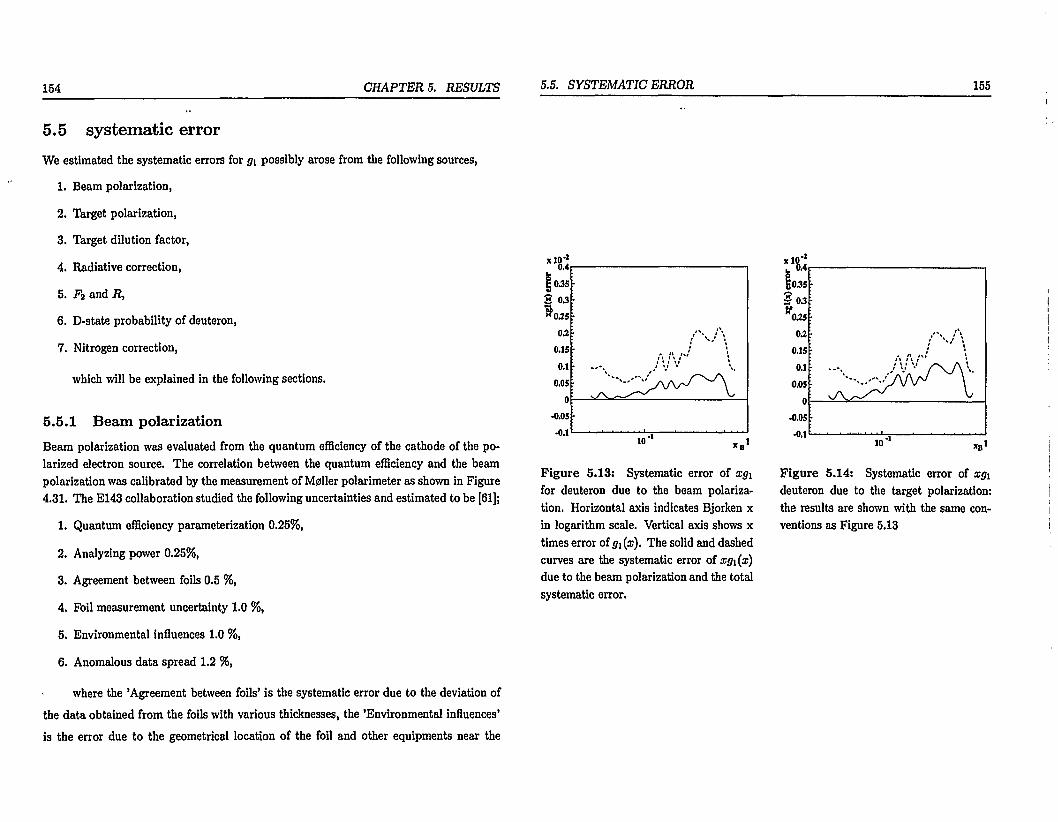
154 CHAPTER 5. RESULTS
5.5 systematic error We estimated the systematic errors for & possibly arose from the following sources,
1. Beam polarization,
2. Target polarization,
3. Target dilution factor,
4. Radiative correction,
5. F 2 and R,
6. D-state probability of deuteron,
7. Nitrogen correction,
which will be explained in the following sections.
5.5.1 Beam polarization Beam polarization was evaluated from the quantum efficiency of the cathode of the polarized electron source. The correlation between the quantum efficiency and the beam polarization was calibrated by the measurement of M0ller polarimeter as shown in Figure 4.31. The E143 collaboration studied the following uncertainties and estimated to be [61];
1. Quantum efficiency parameterization 0.25%,
2. Analyzing power 0.25%,
3. Agreement between foils 0.5 %,
4. Foil measurement uncertainty 1.0 %,
5. Environmental influences 1.0 %,
6. Anomalous data spread 1.2 %,
where the 'Agreement between foils' is the systematic error due to the deviation of the data obtained from the foils with various thicknesses, the 'Environmental influences' is the error due to the geometrical location of the foil and other equipments near the
5.5. SYSTEMATIC ERROR 155
Figure 5.13: Systematic error of xgi for deuteron due to the beam polarization. Horizontal axis indicates Bjorken x in logarithm scale. Vertical axis shows x times error of gi(x). The solid and dashed curves are the systematic error of xgi(x) due to the beam polarization and the total systematic error.
Figure 5.14: Systematic error of xg% deuteron due to the target polarization: the results are shown with the same conventions as Figure 5.13
156 CHAPTER 5. RESULTS
foil target. The total uncertainty of the beam polarization was estimated to be 2.0% in absolute. Because the beam polarization was 84 ~ 86% typically, the fractional error, SPb/Pt, was to be 2.4%. The error of <?i due to the uncertainty of the beam polarization was estimated by using,
ta(«)-^^(4-J«)§. (5-10)
where we neglect of the error of Ax because this error is suppressed by the factor of tan{0/2) which is 0.04 for 4.5° spectrometer and 0.06 for 7° spectrometer. The .<4||-.RC is the cross section asymmetry including any higher order and radiative process, ie. the cross section asymmetry measured actually. Because the radiative correction is independent of the beam polarization, we subtracted the radiative correction from the A\\.
Figure 5.13 shows the beam polarization uncertainty of x5gi(x) for deuteron. The solid curve shows the error of xgi(x) due to the beam polarization and the dashed line is the total systematic error of xgi(x). Because the x axis is in logarithm scale, the gi(x) integral over x is proportional to the area of xgi(x) in this figure, that is
gi{x)dx = xgi(x)d(\ogx). (5-11)
Therefore, the plot of the error of xgi (x) in logarithm scale is good to see the contribution of the error to the integral of g\(x).
5.5.2 Target polarization
The target polarization was extracted from the measurement of the NMR signal calibrated by thermal equilibrium signal which corresponds to polarization by the Boltzmann distribution. The statistical error of the thermal equilibrium measurement dominated the uncertainty of the target polarization which was estimated to be 4.0% for the deuteron target [50],
^ = 0.040 (5.12)
5.5. SYSTEMATIC ERROR 157
The error of gi was calculated with Equation (5.10) substituting Pt for Pj,. Figure 5.14 shows the systematic error of xgi (x) for deuteron due to the uncertainty of the target polarization with the conventions same as those in Figure 5.13.
5.5.3 Dilution factor
The dilution factor is defined to be the fraction of events from the polarized deuteron in the target to the total events. The error of the dilution factor was calculated from the following sources;
1. The coefficient of the EMC effect — the ratio of the cross section of a nuclear per nucleon with respect to that of the deuteron. The uncertainty of the EMC coefficient was estimated from 0.3 to 1.3% relative depending on x [53]. We assigned the EMC effect uncertainty conservatively to be 1.5% over all x.
2. Cross section ratio — The ratio ai/ap has 2.0% uncertainty relative to itself [62].
3. NMR coil uncertainty — The NMR coil uncertainty is due to the lack of knowledge of how much wire exist in the target effectively. We assumed it had 20% relative error [63].,
4. Packing fraction — The packing fraction is a percentage filled by the ammonia beads in the target cell. The packing fraction error depends on the target cell. We used the error of the most frequently used one, which is 2.0% [64].
5. Material weight — We included also the absolute uncertainties in the weight of the ammonia and helium in the target which we assumed to be 4% relative. [65].
Figure 5.15 shows the systematic error of xgf (x) due to the dilution factor.
5.5.4 Radiative correction
The radiative correction gives the uncertainty of gf(x). Only the uncertainty of the
radiative correction for the A\\(x) was included because that for A±(x) was suppressed

158 CHAPTER 5. RESULTS
Figure 5.15: The systematic error of xg\ of deuteron due to the dilution factor: the results are shown by the solid curve. The dashed curve is the total of the systematic error.
Figure 5.16: The systematic error of xg^(x) due to the radiative correction: only the uncertainty on the correction for J4|| was accounted. The results are shown with the same conventions as Figure 5.15
by the small factor tan 9/2 as shown in Equation (5.5). The uncertainty of the radiative correction was evaluated with a varying of input models and the error of the data points. The error of g*(x) due to the radiative correction was calculated by,
55i = §«*C, (5.13)
where SRC is the uncertainty of the radiative correction for the J4||. Figure 5.16 shows
the error of xgf(x).
5.5.5 Total cross sect ion
F\/D' in Equation (5.5) has an uncertainty due to the error of the spin-averaged structure functions. This uncertainty contributes to the systematic error of gf(x).
F\/D' in Equation (5.5) is expressed in terms of F2 and R by,
F1 _ ( l - t - 7
2 )y(l + 6fl) D> 22x(l + R){l-e){2-yy (5.14)
5.5. SYSTEMATIC ERROR 159
and in terms of the total cross section by [22],
D' <rM o«2(2-j/)tan 2(^/2)' ^ 0 )
where a is the total cross section, OMOU is the Mott cross section given by,
_ ,4a ' (S ' )W(g /2 ) OMM — Q4 • (5.16;
In principle, the uncertainty ofFi/D1 calculated by using Equation (5.15) or (5.14) should be identical. On the other hand, the uncertainty calculated by using the Equation (5.14) without any account for a correlation between the errors of F2 and R is larger than that calculated by using the Equation (5.15) because the accuracy of the total cross section is nearly equal to that for F2. Therefore, the proper way to calculate the uncertainty of F\/jy is either using Equation (5.14) accounting the correlation between the errors of F2
and R or using the Equation (5.15). We calculated the error of F\fD' by using Equation (5.15).
We assumed that the fractional uncertainty of the total cross section is same as that of F2. We estimated the uncertainty of the F2 using two FORTRAN codes, F2GLOB.F and F2NMC.F. F2GLOB.F provides the F2 for various kinematic region from a fit using results of past SLAC experiments [62]. It also gives the statistical, systematic, and normalization errors evaluated from the experimental results. F2NMC.F provides F2 with NMC parameterization [59] which was obtained from the NMC muon-nucleon scattering. F2NMC.F is more reliable than F2GLOB.F in low x region due to the availability of the data used to determine the parameters.
The error of F2 was calculated by,
~w i \~w)+ + v w™)' (5 ,17)
where F2'tat is the statistical error which was provided by F2GLOB.F, norm is a normal
ization uncertainty 1.7% which was derived from Ref.[62], and the last term comes from
the model dependence. Using the fractional error of F2, the systematic error of gi due to

160 CHAPTER 5. RESULTS
the total cross section is given by,
The last term in Equation (5.17) gives a huge uncertainty in the low x region of x < 0.08 because of large discrepancy between F2(x) obtained from F2GLOB.F and F2NMC.F. It is an obvious over-estimation for the error because the NMC parameterization is more reliable at low x than F2GLOB. F2GLOB states that the routine is not useful in the region of x < 0.08 due to the poor statistics in the fit.
Figure 5.17 shows F2(x) data from the NMC experiment and the parameterization curve at Q2 = 3.0(GeV/c)2[59]. Only the data obtained at Q2 between 2.5 and 3.5 (GeV/c)2 are plotted. The two dotted lines indicate the band within 4% relative uncertainty from the parameterization curve. This relative uncertainty of 4% is acceptable for the F2 error in the low x region from the figure. Therefore, we took that F2 has the relative uncertainty of 4% in the region of x < 0.08.
Figure 5.18 shows the error of xgf(x) due to the uncertainty of F\/D'.
5.5.6 D-state probability
The D-state probability, wo is a fraction of the deuteron in D-state (L=2) as mentioned in Section 2.5. It was estimated from the calculation using various models to be 5.5 ~ 6.5%[28] and we assigned to be wo = 6 ± 1% which covers all of the results. This uncertainty causes an ambiguity of the g\ not for deuteron but for neutron and proton -neutron showing Equations (5.8) and (5.9). The uncertainties of T" and r p - T" due to the D-state probability are 3% of Td.
5.5.7 Nitrogen correction
Nitrogen correction is a correction due to the polarized nucleon other than deuteron in the target. This is a small correction and the uncertainty of the correction factors are negligible for the cross section asymmetry or gi (x) as stated in Section 4.2.5. The nitrogen
5.5. SYSTEMATIC ERROR 161
Figure 5.17: F2 data from NMC experiment and the parameterization curve. Only the data between Q2 = 2.5(GeV/c)2
and Q2 = 3.5(GeV/c)2 are plotted. The dotted lines show the band within the relative uncertainty of 4% from the parameterization curve.
Figure 5.18: Systematic error of xgd(x) due to the Fi/D': the solid curve shows the result. The dashed curve is the total of the systematic errors of xg\(x).

162 CHAPTER 5. RESULTS
correction for the cross section asymmetry is expressed to be,
A A-i • M j (5.19) V\ [PdPdf
where v\ and v2 are the correction factors which are approximately 0.98 and 0.06 respectively and Ap is the cross section asymmetry for proton. Although the uncertainties for the v\ and u2 are negligible, the error of the cross section asymmetry of the proton in the correction may affect due to the large magnitude of the asymmetry for proton in contrast to that for deuteron. Therefore, we estimated the uncertainty due to the proton asymmetry by
^ = § 2 M " (5-2°) where 6AP is the statistical error of the proton asymmetry. We calculated only the uncertainty from the A\\ due to the proton asymmetry.
The uncertainty of r d due to the error of Ap was estimated to be 0.0001 which was smaller than ten times of the other error, for example 0.0016 for the dilution factor and then it was negligible to the Td.
5.6 Integrals of g\(x)
We first calculated the integral of 51 (a;) over the data region of 0.029 < a; < 0.8. To estimate the shape of gi(x) in the outside of the data region where (0.8 < x < 1) and (0 < x < 0.029), we used the extrapolation for g\{x) towards x = 1 and x = 0 respectively.
5.6.1 integral in data region
We calculated the integral of gu Tjata over the data region of 0.029 < x < 0.8 using the
rectangle approximation of,
Tdaia = I > i (xi) x Aar{, (5.21)
5.6. INTEGRALS OFGi(X) 163
where i is the index for the bin, Aa;* is the size of the bin. The statistical error, ST^b was calculated by,
(Srffi) 2 = £ {SgW1 x Az<}2, (5.22) i
where 5gi(xi)'M is the statistical error of gifa). The total systematic error, SV'J^ was calculated by,
« , ) 2 = £ i I i X>, (as,)?'Aa,
T2 (5.23)
where j is the index for the source of the systematic error, 5g\{xi)'^' is the uncertainty of gi due to the systematic error. The systematic errors of g\{x) for different bins from the same source are correlated to each other. We therefore summed the error on all bins linearly as shown in Equation (5.23). The results of r ^ o . <5r& and <$r$[|0 are shown in Table 5.4.
gi 5? s?-sr 0.0384 0.0035 0.0036
-.0326 0.0083 0.0095
0.1495 0.0103 0.0142
Table 5.4: Integral of g\{x) on the data region: The integral of g\{x) for deuteron, neutron, and proton - neutron in the region of 0.029 < x < 0.8 are shown.
5.6.2 Low x extrapolation
Because our measurement reached down to x=0.029, we had to estimate the g\ for a; < 0.029. In such a low x region, sea quarks dominate the scattering and the information of the initial parton spin is then lost by the gluon emission. According to Regge theory[66] 51 approaches to 0 at the low x region and is proportional to xa with 0 < a < 0.5, where the a is the Regge intercept at t = 0.
In the past experiments, the spin-averaged structure function Fi(x) has been measured down to a lower x region with higher accuracy than the spin structure function, gi(x).

164 CHAPTER 5. RESULTS
These experiments showed that the spin-averaged structure function is described by the Regge theory in such a low x region. The Figure 5.19 shows the Fz(x) for deuteron from NMC, where only the data taken between Q2 = 2.5(GeV/cf and Q2 = 3.5(GeVr/c)2 are plotted. The solid line shows the NMC parameterization for Fi(x) at Q2 = 3.0((7eV/c)2. The dash-dotted line show the reduced x 2 if we involve the data into the Regge form fitting up to there. The evolution of the reduced x 2 demonstrated that the fit by the Regge form is acceptable up to around x = 0.1.
—. 0.4 3 <3,0.38 to
0.36 0.34 0.32
0.3
0.28
0.26
0.24
0.22
0.2
Figure 5il9: F2 from NMC in the region between 2.5 < Q2 < 3.5(GeV/c)2. The left y-axis shows the F% and the right-hand y-axis shows the reduced x 2 . The solid line shows NMC parameterization at Q2 = 3.0(GeV/c)2. The dashed line shows the reduced x 2 for the fit with the data up to there. The fit was done with two parameters pxxfi suggested by Regge theory.
Therefore, assuming that g\ was proportional to xa in the low x region of x < 0.1, we fitted the Regge forms with three fixed a of 0, 0.25 and 0.5 to the data up to x=0.1. Figures 5.20, 5.21, and 5.22 show the low x fits for g{, g?, and flf - fl" respectively. All of these fitting curves do not describe the data well. However since the contribution to the integral from the low-x region is small, we took the shape of gi(x) determined by the
X n
5.6. INTEGRALS OF Gt(X) 165
Is °-3
0.25 0.2
C I S O . l
O.OS
O
- 0 . 0 5 -O.l
- 0 . 15 _ < K 2 0 0 .02 0 .04 <M>6 0 .08 OTI 0 0 2 0 . 1 4
* B
Figure 5.20: Extrapolation toward x = 0 for gx of deuteron with Regge form. The dotted, solid, and dashed lines show the fits with the forms of Cx°, Cx0i2S, and CxM
where C is a fitting parameter. These fits were done using the data up to a=0.1.
f 0 t
>
i i 'UL I t t f 0 t """ " o f T
' > i i 1 r i •
1 •
1 . . . 1 . . . 1 . . . . . . . 1 . . . 1 .
fit with a = 0.25 and calculated the integral,
/•0.029 Ito. = / Cx°™dx, Jo (5.24)
where C is the parameter determined from the fit.
To estimate the uncertainties in the low-x region, we considered the statistical and systematic errors of the data points, uncertainty of the parameter a and the data region used in the fit.
The statistical error of the extrapolation, STf^ was calculated by,
r0.029
Jo
fO.029
«rjaf=/ scx°-Kdx, Jo
(5.25)
where SC is the error of the fitting parameter.
For the systematic error, we assume that the fitted curve has the fractional uncer
tainty same as the average of the fractional systematic error of the data points, Sg{y' and

166 CHAPTER 5. RESULTS
- 0 . 6 O 0 . 0 2 0 .04 0 . 0 6 0 . 0 8 0 .1 0 . 1 2 0 . 1 4 * B
Figure 5.21: Extrapolation toward x=0 of 51 of neutron. The fitted curves are indicated with the same conventions as Figure 5.20.
Figure 5.22: Extrapolation toward x=0 of 5?—£"• The fitted curves are indicated with the same conventions as Figure 5.20.
5.6. INTEGRALS OF Gi(X) 167
calculated the systematic error of the extrapolation, 6T'Z
SrZ = Wj°'m Cz™dx, (5.26)
where C is the fitted parameter with a = 0.25.
The uncertainty of the extrapolation due to the parameter a was estimated to be the largest difference in r ^ with 0! = 0| or a = 0.5 from that with a + 0.25.
The uncertainty due to the fitted region was evaluated by varying the upper limit from x = 0.05 to 0.13 corresponding to the first 5 to 13 data points. The largest difference in Tfou, from that obtained at the upper limit of a;=0.1 was taken as the uncertainty due to the fitting region.
Table 5.5 shows the summary of the integral and the errors of the low x integral. The STf^ is the quadratic sum of the uncertainties due to the parameter a and the fitted region.
9i 9? tf-fc" Mow 0.0011
0.0003 0.0002 0.0008
-0.0030 0.0007 0.0005 0.0028
0.0084 0.0009 0.0008 0.0059
fitting parameter error of parameter
Reduced x 2
0.11 0.03 0.66
-0.32 0.08 1.01
0.88 0.09 1.23
Table 5.5: Integral of g\ in the low x region, 0 < x < 0.029: The extrapolations were determined from the fits using the Regge form with a = 0.25 with the data up to x = 0.1. The <$r,*k,' is the uncertainty due to the error of the fitted parameter. The 6r'Z is the uncertainty due to the systematic error of the data which were used by the fit. The 6r{£, was the quadratic sum of the uncertainties due to the Regge parameter a and the variation of the fitting region.
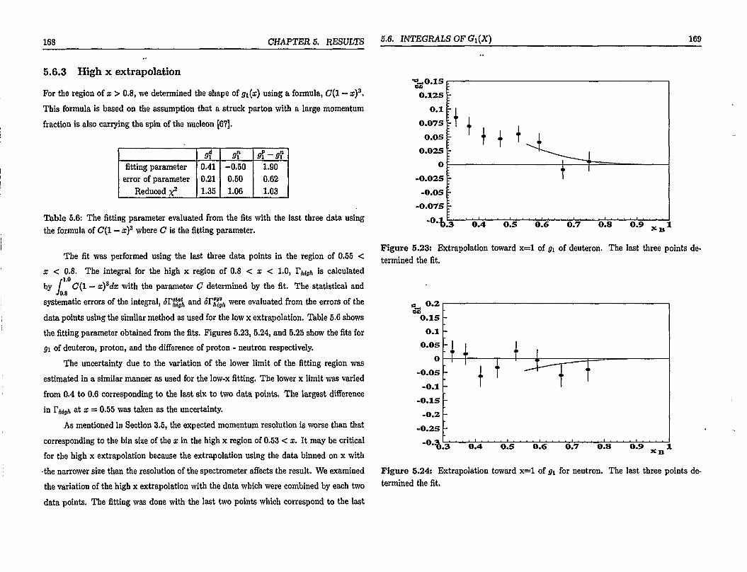
168 CHAPTER 5. RESULTS
5.6.3 High x extrapolation
For the region of x > 0.8, we determined the shape of gi(x) using a formula, C(l - x)3. This formula is based on the assumption that a struck parton with a large momentum fraction is also carrying the spin of the nucleon [67].
9i fl? *r-*r fitting parameter
error of parameter Reduced x 2
0.41 0.21 1.35
-0.50 0.50 1.06
1.90 0.62 1.03
Table 5.6: The fitting parameter evaluated from the fits with the last three data using the formula of (7(1 - x)3 where C is the fitting parameter.
The fit was performed using the last three data points in the region of 0.55 < x < 0.8. The integral for the high x region of 0.8 < x < 1.0, Thigh is calculated
rl.O by / C(l — x)3dx with the parameter G determined by the fit. The statistical and
J0.8
systematic errors of the integral, ST^ and <Srj$*A were evaluated from the errors of the data points using the similar method as used for the low x extrapolation. Table 5.6 shows the fitting parameter obtained from the fits. Figures 5.23, 5.24, and 5.25 show the fits for Pi of deuteron, proton, and the difference of proton - neutron respectively.
The uncertainty due to the variation of the lower limit of the fitting region was estimated in a similar manner as used for the low-x fitting. The lower x limit was varied from 0.4 to 0.6 corresponding to the last six to two data points. The largest difference in Thigh at a; = 0.55 was taken as the uncertainty.
As mentioned in Section 3.5, the expected momentum resolution is worse than that corresponding to the bin size of the x in the high x region of 0.53 < x. It may be critical for the high x extrapolation because the extrapolation using the data binned on x with •the narrower size than the resolution of the spectrometer affects the result. We examined the variation of the high x extrapolation with the data which were combined by each two data points. The fitting was done with the last two points which correspond to the last
5.6. INTEGRALS OF Gi(X) 169
"H-,0.15 0.125
O.lf-0.075
0.05 0.025
O -0.025
-0.05 -0.075
It
0.4 0 .5 0.6 0.7 0.8 0.9 .. 1 X B
Figure 6.23: Extrapolation toward x=l of gi of deuteron. The last three points determined the fit.
Figure 5.24: Extrapolation toward x=l of ffi for neutron. The last three points determined the fit.

170 CHAPTER 5. RESULTS
Figure 5.25: Extrapolation toward x=l on g\(x) — gx(x). The last three data points determined the fit.
four data in the original data array. The deviation of the integral from that obtained using the original data was accounted as one of the systematic error.
The Table 5.7 shows the summary of the integrals of gt for deuteron, neutron, and proton - neutron in the region of 0.8 < x < 1.0 obtained from the extrapolations. The ($r{}jh is the quadratic sum of the uncertainties due to the variation of the fitting region and the bin size of the data used to determine the fit.
5.7 Test of the sum rules The complete integral of gi(x) in the region of 0 < x < 1, T was obtained by combining
the results of the three regions as,
T = Flow + Tdoto + Thigh.
The statistical errors in the three regions were combined quadratically by,
(5.27)
5.7. TEST OF THE SUM RULES 171
at 5? Sf-Sf r/or(0.8 < x < 1) 0.0002 -0.0002 0.0008
srffih 0.0001 0.0002 0.0003 ^hi'gh 0.0000 0.0000 0.0001 With 0.0002 0.0005 0.0006
Table 5.7: Integral of g\(x) in the high x region of 0.8 < x < 1.0 were evaluated from the extrapolation toward x = 1. The statistical error of the integral, SFf^h *s the uncertainty due to the statistical error of the data points. The systematic error, 5rhfgh is the uncertainty due to the systematic error of the data points. 5rj$Jh is the quadratic sum of the the uncertainties due to the variation of the fitting region and the bin size of the data used to determine the fit.
where the STatttt is the statistical error of the complete integral. The systematic errors in the three regions were combined linearly. The uncertainty of the fit in the low and high x regions, 6T{£, and 6rf
hfgh were included into the total systematic error, 6F'y' as,
sr>»> = Jfrz+ax,+8rh%hf + {srZf + (arj™,,)2. (5.29) Table 5.8 shows the integrals of gi at Q2 = 3.0((?eV/c)2 with the statistical and
systematic errors. The lower part of the rows shows the contributions from the various uncertainties to the total systematic error.
We also calculated the integrals of g\(x) at Q2 = 10.0(GeV/c)2 to compare to the results from Spin Muon Collaboration (SMC) under the assumption that gi/Fi was independent of Q2. Table 5.9 shows the T at Q2 = 10.0(GeV/c)2. The statistical and the systematic errors were calculated in the same procedure as used for the calculation at Q2 = 3.0(GeV/c)2.
5.7.1 Ellis-Jaffe sum rule for deuteron
As shown in the Table 5.8, the gi(x) integral for deuteron at Q2 = 3.0(GeV/c)2 was
evaluated as,
F1 = 0.0396 ± 0.0035(s«ai.) ± 0.0039(sys*.), (5.30)

172 CHAPTER 5. RESULTS
at fl? flf-tf r 0.0396 -.0358 0.1586
fiptat 0.0035 0.0084 0.0103 Beam polarization 0.0011 0.0008 0.0039 Target polarization 0.0016 0.0049 0.0071
Dilution factor 0.0016 0.0054 0.0079 py» Radiative correction 0.0024 0.0057 0.0068
Fi/ff 0.0009 0.0022 0.0053 D-state probability - 0.0012 0.0012
Low x extrapolation 0.0009 0.0030 0.0060 High x extrapolation 0.0002 0.0005 0.0007
Total 0.0039 0.0105 0.0162
Table 5.8: Integral of g\ in the region of 0 < x < 1 at Q2 = 3.0(GeV/c)2: contributions to the systematic error from each source are shown in the lower part of the table.
gi 3? tf-tf r/or(0 < x < 1) Statistical error Systematic error
0.0400 0.0030 0.0041
-0.0380 0.0073 0.0115
0.1641 0.0089 0.0183
Table 5.9: Integral of fli in the region of 0 < x < 1 at Q2 = 10.0((7eV/c)2. The results were evaluated under the assumption that g1(x)/F\(x) is independent of Q2.
5.7. TEST OF THE SUM RULES 173
where the first error is the statistical error and the second error is the systematic error. The theoretical prediction including the QCD correction up to third order of the a, — 0.36 db 0.05 [27] at Q2 = 3.0(<?eV7c)2 is,
Td = 0.068 ± 0.005, (5.31)
with the D-state probability of deuteron WD = 0.06. r d from the B143 experiment differs from that of the Ellis-Jaffe sum rule for deuteron by about four standard deviations, where the standard deviation was taken as a quadratic sum of the statistical and systematic errors of the integral and the uncertainty in the Bllis-Jaffe sum rule.
In order to verify the consistency of our results to those from SMC, we calculated the gx (x) for deuteron at Q2 = 10.0(GeV/c)2. The results of xgd(x) from E143 and SMC are plotted in Figure 5.26 together. The closed and open circles show the xgi(x) for deuteron from E143 and SMC respectively. The error bars are only statistical. The dark and open areas indicate the size of the systematic errors for E143 and SMC respectively. These results are in a good agreement to each other in the overlapped region.
These results are summarized together with the theoretical prediction from the Ellis-Jaffe sum rule at Q2 = 10.0{GeV/c)2,
Td = 0.0400 ±0.0030(sio«.)± 0.0041 (syst.) : £143,
r d = 0.034 ± 0.009{stat.) ± 0.006(sysi.) : SMC,
Td = 0.070 ±0.004 -.theory, (5.32)
showing that r d from E143 at Q2 = 10.0{GeV/c)2 is consistent to that from SMC. However, the r d predicted by the Ellis-Jaffe sum rule is different from both of the experimental results by more than three standard deviations.
The Figure 5.27 illustrates the comparison of the Td measurements and the theoretical prediction as a function of Q2. The closed and open circles show the results from E143 and SMC at Q2 = 3.0 and 10.0(GeV/c)2 respectively. The error bars are the quadratic sum of the statistical and systematic errors. The solid line shows the theoretical prediction including the QCD correction up to third order of as(Q2). The Q2

174 CHAPTER 5. RESULTS
Figure 5.26: xgi of deuteron: the results from E143 and SMC are plotted together by the open and closed circles respectively. Both results were evaluated at the common Q 2 = 10.0(GeV/c)2. The error bars are statistical only. The dark and open areas indicate the size of the systematic errors for E143 and SMC respectively.
5.7. TEST OF THE SUM RULES 175
10 12 Q 2 (GeV/c) 2
Figure 5.27: Td with the prediction of the Ellis-JafFe sum rule: The horizontal axis shows Q2 and the vertical axis shows P*. The open and closed circles indicate the results from E143 and SMC respectively. The error bars are the quadratic sum of the statistical and systematic errors. The solid line shows the prediction of the Ellis-Jaffe sum rule up to third order of aa. The dotted lines show the band within one standard deviation from the prediction.

176 CHAPTER 5. RESULTS
evolution of the prediction was calculated using the running strong coupling constant, aa(Q2) with A<n'=4> = 0.364 ± 0.052 GeV which was evaluated in Section 5.7.3, where n/ is the number of quark flavors. The dotted lines show the band within one standard deviation from the prediction. The uncertainty of the prediction was calculated from the errors of the A^nf~4\ hyperon decay constants, F and D, and the D-state probability of the deuteron. The results from both experiments indicate a large discrepancy of more than three standard deviation from the prediction.
5.7.2 Ellis-Jaffe sum rule for neutron
-0.6 c • '— ' « • ' ' — ' 10 1
Figure 5.28: The gi of neutron from E143 and E142 are plotted together by the open and closed circles respectively. Both results were evaluated at the common Q2 = 2.0(GeV/c)2. The error bars are statistical only. The dark and open areas indicate the size of the systematic errors for E143 and E142 respectively.
5.7. TEST OF THE SUM RULES 177
So
xlO"' O
-O.S
3-1-51 -2
-2.5
-3
-3.5
-4
-4.5
-5
\ E142 <
*»
\ E142 < »
6 E143
• • • • • i • • •
0 8 , 1 0 , Q 2 (GeV/c) 2
12
Figure 5.29: Tn results with the prediction of the Ellis-Jaffe sum rule: The horizontal axis shows Q2 and the vertical axis shows Tn. The open and closed circles indicate the results from E143 and E142 respectively. The error bars are the quadratic sum of the statistical and the systematic errors. The solid line shows the prediction of the Ellis-Jaffe sum rule up to third order of at. The dotted lines show the band within one standard deviation from the prediction.

178 CHAPTER 5. RESULTS
The T for the neutron at Q2 = 3.0((7eV/c)2 using our deuteron and proton results was
obtained to be,
r n ( Q 2 = 3.0) = -0.0358 ± 0.0084(s<a<.) ± 0.0105(sys.). (5.33)
This result indicates a discrepancy from the prediction of the Ellis-Jaffe sum rule for
neutron,
P*(Q2 = 3.0) = -0.009 ± 0.006 : theory, (5.34)
by 1.8 times of the standard deviation. Figure 5.28 shows the g\ (x) for neutron at Q2 = 2.0(GeV/c)2. The closed and open
circles show the 9i(x) obtained from E143 and E142 [12] respectively. These results are in a good agreement to each other.
Figure 5.29 shows r n from E143 and E142 with the predicted curve by Ellis-JafFe sum rule including the QCD correction up to third order of a, as a function of Q2. The Q2 evolution of the prediction was calculated using the running strong coupling constant, a,(Q 2) with A(n'=4) = 0.364 ± 0.052GeV which was evaluated in the next section. The error bars are the quadratic sum of the statistical and systematic errors. The results from E143 and E142 which are shown by the open and solid circles are in a good agreement and lower than the prediction. However, the accuracies of the results are not enough to exclude the Ellis-Jaffe sum rule for neutron.
5.7.3 Bjorken sum rule
The difference of the integrals of tf(x) and g?(x), W - Tn are obtained from Table 5.8
to be,
T" - Tn(Q2 = 3.0) = 0.1586 ± 0.0103(stat.) ± 0.0162(sys.), (5.35)
which is consistent with the prediction from the Bjorken sum rule at Q2 = 3.0 (GeV/c)2
given by,
V - Tn{Q2 - 3.0) = 0.169 ± 0.008 : theory. (5.36)
5.7. TEST OF THE SUM RULES 179
Figure 5.30: xg\—xg%: the closed and open circle show the results at Q2 — 10.0((?eV/c)2
from E143 and SMC [16] respectively. The error bars are only statistical. The closed and open areas show the size of the systematic errors for E143 and SMC results.

180 CHAPTER 5. RESULTS
We evaluated the c?(x) - g?{x) at Q 2 = 10.0(GeV/c)2 for comparison to the SMC results. These two data are consistent with each other as shown in Figure 5.30. The integrals from these measurements are,
I* - r n ( Q 2 = 10.0) = 0.1641 ± 0.0089(stat.) ± 0M83(sys.) : £143 (5.37)
V - r n ( Q 2 = 10.0) = 0.199 ±0.038 : SMC (5.38)
where the error of the SMC result contains both of the statistical and systematic errors [16]. The two results are in good agreement with the prediction of the Bjorken sum rule at Q2 = 10.0(GeV/c)2 given by,
F P _ r»(Q2 = 1 Q 0 ) _ 0 l g 7 ± 0 0 0 3 . t h e o r y p (5,39)
The Figure 5.31 shows the comparison of the r p - Tn measurements and the theoretical prediction as a function of Q2. The solid and open circles show the results from E143 and SMC at the averaged Q2 respectively. The solid line shows the theoretical prediction including the QCD correction up to third order of as(Q2). The dotted lines show the band within one standard deviation from the prediction. The uncertainty of the prediction was calculated from the errors of the A( n/ = 4) and the hyperon decay constants, F and D. The results from both experiments are in good agreement with the prediction.
Figure 5.32 shows the strong coupling constants obtained from the various experiments. Using the measurement of V — T", we calculated the strong coupling constant a,(Q2 = 3.0) to be 0.417+g;Jf§ with the Equation (2.72) and plotted as the open circle. The closed triangle is the average of the results of r decay measurements by Particle Data Group (PDG) [26]. The closed square is the NMC result obtained from the measurements for the scaling violation of the spin-averaged nucleon structure function [68]. The closed circle is the result of CCFR obtained from the measurement for the Gross-Llewellyn Smith sum rule [69]. The solid curve is the running coupling constant, a,(Q2) obtained from the fitting using these data plotted in the figure. We used the renormal-ization scheme with the number of flavor, n/ = 4 to obtain the running strong coupling
5.7. TEST OF THE SUM RULES 181
0.24
tT 0.22
0.2 h
0.18
0.16
0.14
0.12
0.1, 0
SMC
-'9 E143
10 Q 2 (GeV/c ) 2
12
Figure 5.31: T p - T" with the prediction of the Bjorken sum rule: The horizontal axis shows Q2 and the vertical axis shows P - P * . The open and closed circles show the results from E143 and SMC respectively. The error bars are the quadratic sum of the statistical and systematic errors. The solid line shows the prediction of the Bjorken sum rule up to third order of or,. The dotted lines show the band within one standard deviation from the prediction.

182 CHAPTER 5. RESULTS
constant. The data were fitted to the formula of [26]
a.(Q2) •• \2ir
(33-2n/)log(QVA 2) 1 -6(153 -lVnf)\og[\og{Q2ltf)\\
(33 - 2n/)2 log(Q7A2) (5.40)
where A is the parameter determined to be 0.364 ±0.052 GeV by the fitting. The reduced X2 of the fit was 0.33. This running coupling constant was used to obtain the 0} evolution of the sum rules shown in Figures 5.27, 5.29, and 5.31.
0.5 •
0.4
0.3 'it — ^——_
i
0.2 '
o E143 0.1 A x decay (PDG)
'_ • NMC • CCFR
0.0 . . . J — l i 1 1 1 1 1 1 1 L—J 1 1 1 1 1 1 1—-1.- J 1 1 — L—
0 2 4 6 8 10 12 Q 2 (GeV/c) 2
Figure 5.32: The strong coupling constant a, as a function of Q 2. The open circle is the result from E143. The closed triangle is the result obtained from the decay width of the T lepton [26]. The closed circle is the result from NMC [68] obtained by the measurement for the scaling violation of the spin-averaged nucleon structure function. The closed circle is the result from CCFR [69] obtained by the measurement for the Gross-Llewellyn Smith sum rule. The solid line and the dotted lines show the running coupling constant and the "band within one standard deviation obtained by the fit using these data.
5.8. QUARK POLARIZATION 183
5.8 Quark polarization
We calculated the quark polarization with Td by using the Equation (2.87). We found the quark polarization to be,
Au = 0.822 ±0.019, Ad = -0.435 ±0.019, As = -0.101 ±0.023,
A E = Au + Ad + As = 0.286 ±0.055, (5.41)
where the errors include both of statistical and systematic uncertainties of I"*, the error of D-state probability on the deuteron, uncertainties of axial vector couplings, and the error of the strong coupling constant in the QCD correction. These results demonstrate that the strange quark is polarized significantly opposite to the nucleon spin and the total quark polarization is about 30% of that for the nucleon; indicating that a large portion of the nucleon spin is still missing.
Figure 5.33 shows the strange quark polarizations as a function of the total quark polarization from various experiments. We recalculated the quark polarizations from EMC[11] and E142[12] with the QCD correction up to third order of a, [27]. The values from the E143 deuteron measurement is in good agreement with the other results with the highest accuracy among these measurements. The averages of the quark polarizations were calculated to be
As = -0.103 ±0.015, (5.42)
Au + Ad + As = 0.279 ±0.039, (5.43)
indicating again that the strange quark is polarized significantly opposite with respect to the nucleon spin and the quark carries only about 30% of the nucleon spin. These results denote that the assumption of the unpolarized strange quark to derive the Ellis-Jaffe sum rule is invalid and reconfirmed the 'spin crisis' with the higher accuracy than those obtained before.

184 CHAPTER 5. RESULTS
-0.2 -
Au+Ad+As
Figure 5.33: The quark polarization evaluated from various experiments are plotted. The horizontal and vertical axes show the total quark polarization and the strange quark polarization. The shaded areas indicate the band within one standard deviation from the average of the polarizations, As = -0.103 ± 0.015 and Au + Ad + As = 0.279 ± 0.039.
Chapter 6
Conclusion and a look into the future
We have measured the deuteron spin structure function gi (x) in the E143 experiment at SLAC using the highly polarized electron beam and the highly polarized frozen ND& target. The experiment provided the high precision data for the structure function from x =0.029 to 0.8. The integral of the spin structure function gi for deuteron over x at the averaged Q2 = Z.0(GeV/c)2 and the prediction from the Ellis-Jaffe sum rule were found to be,
Experiment Td = 0.0396 ±0.0035(stai.)±0.0039(sj/s.), (6.1)
Theory Td = 0.068 ±0.005. (6.2)
The result indicate that the Ellis-Jaffe sum rule describes the data improperly. It denotes that the assumption to derive the Ellis-Jaffe sum rule which is the unpolarized strange sea quark, is not valid.
Combining the E143 deuteron and proton data [18], we obtained the difference of the integrals, I* - P . The V - Tn from this experiment and the prediction by the Bjorken sum rule are to be,
Experiment r p - T" = 0.1586 ±0.0103(stat.)±0.0162(sys.), (6.3)
Theory Tp~Tn = 0.169 ±0.008. (6.4)
From these results, we confirmed that the Bjorken sum rule gives a consistency to the
185

186 CHAPTER 6. CONCLUSION AND A LOOK INTO THE FUTURE
experimental results at Q2 = 3.0(GeV/c)2 with the high accuracy. It means that Iso Spin symmetry is valid for the spin structure function g\ for nucleon and the Perturbative QCD well describes the scaling violation of the spin structure function.
Strong coupling constant a, at Q2 — 3.0(GeV/c)2 was evaluated by using up to the third order of QCD correction for the Bjorken sum rule to be,
a,(Q2 = 3.0(GeV/cf) = 0.417+858, (6.5)
giving the consistency with the other measurements. Quark polarization for each flavor was calculated using our deuteron data and
hyperon decay constants under the assumption of flavor SU(3). The polarization of strange quark was found to be significantly negative, As = —0.101 ± 0.023, suggesting that the assumption of the Ellis-Jaffe sum rule that the strange quark in nucleon is unpolarized, is incorrect. The total quark polarization was found to be 0.286 ± 0.055 which is much less than the prediction of 1.0 from the non-relativistic quark model and of 0.65 from the relativistic treat of bag model[70]. Now, 'spin crisis' is not 'crisis' anymore. Our understanding of the nucleon spin had been wrong and we have to establish a new model to describe the spin of the nucleon properly.
Many theoretical works have been carried out to explain the small total quark polarization.
The quark content of the nucleon spin was calculated employing the lattice QCD. M. Fukugita et al.[71] obtained AS = 0.18 ± .10 and As = -.109 ± .030 which is reasonably consistent with our results. S. J. Dong et al. [72] calculated to be AS = 0.25 ± .12 and As = —.12 ± .01 which is also consistent with our results.
A way to salvage the naive quark model of the nucleon, is to introduce a large gluon polarization. The diagram shown in Figure 6.1 causes a gluon contribution to the total quark polarization evaluated from the polarized e-N scattering. Accounting this effect called axial anomaly, the quark polarization evaluated from the polarized e-N scattering, Aq is expressed to be [73]
Aq^Aq-^AG, (6.6)
187
where AG is the gluon polarization. The strong coupling constant a, decreases with the increasing Q2 and AG has Q2 dependence like In Q2 thus the second term of the RHS. of Equation (6.6) does not vanish in the scaling limit of Q2 -)• oo. Therefore, the QCD correction by the power of a, is not valid to correct this anomalous gluon contribution and we measure not the Aq, but the Aq in the e-N scattering. If AG ~ 2, the total quark polarization are corrected to be <$£ ~ 0.6 and As ~ 0 which are consistent to the results of the relativistic treat of the bag model. Of course, this large gluon polarization have to be canceled by the orbital angular momentum to conserve the angular momentum of the nucleon. An advantage of this model is conserving a non-singlet term like Au—Ad in the e-N scattering if the anomalous contribution is identical for three flavors. The Bjorken sum rule is then still valid in this model.
Skyrme model is being discussed recently because this model gives 0 quark polarization. In this model, the quark is interpreted to be asoliton solution of the SU(Nc)xSU(Nf) chiral Lagrangian where Nc and Nf are the numbers of the color and flavor of quarks in the nucleon. Notice that the quark in this model is mass-less. Although the whole of the nucleon spin is carried by the orbital motion of the quarks in this model, an possibility is denoted by Ref.[74] that the 1/7VC expansion and the quark mass correction make the quark carrying < 30% of the nucleon spin which is consistent to the experimental result.
More experiments are needed to make a further understanding of the spin structure of the nucleon. The Q2 dependence and the low-x behavior of the spin structure function are curious to examine the perturbative QCD and to study the higher twist effect.
SLAC-E154 directly measured the spin structure function of neutron using gaseous 3He target which was previously measured in SLAC-E142, but with higher beam polarization and higher energy electron beam than SLAC-E142. This measurement will improves the results of E142 and give the precise data for the neutron spin structure function. E154 ended its measurement in Fall of 1995 and the analysis is in progress.
SLAC-E155 will start in 1996 to measure the spin structure function of proton and deuteron with the 50 GeV polarized electron beam. This 50 GeV electron beam allows us to provide precise data down to lower i than the current SLAC data and to clarify

188 CHAPTER 6. CONCLUSION AND A LOOK INTO THE FUTURE
the low-x behavior of the spin structure function with high accuracy. SMC experiment will keep their measurement for the spin structure function until
1996 and the measurement will decrease the ambiguity of their current results [16] [15] and provide the more precise data of the g\ at low x region due to the high energy beam.
The gluon polarization may be a key to solve the nucleon spin. An exclusive meas-
photon
gluon 1-94 7687A4
Figure 6.1: The Feynman diagram of photon-gluon fusion. The virtual photon and gluon make the quarkonium, qq. The cross section of the interaction is supposed to depend on the gluon and photon helicities. charmonium, J/\£f is the best candidate to tag the interaction because the charm quark is found hardly in the nucleon.
urement is suggested in positron-nucleon or proton-proton scattering to investigate gluon polarization[75]. The production rate for J / * should depend on the gluon polarization in • both cases, because the dominant process of the J/\P production is photon-gluon fusion as shown in Figure 6.1 or gluon-gluon scattering in e-N or NN scattering respectively. The following two projects, HERMES at DESY and Relativistic Hadron and Ion Collider, RHIC at BNL can possibly provide this most interesting measurement for the gluon polarization.
HERMES project[17] at DESY is measuring the polarized positron scattering with many kinds of polarized gaseous target. It has a large detector surrounding the interaction
189
point and the detector allows to study not only the inclusive cross section on a wide kinematical region, but also the exclusive measurement like quark-gluon fusion.
An polarized proton-proton scattering experiment is planed in RHIC at BNL. This experiment will measure the gluon polarization in the nucleon which is not found yet. Fermi National Accelerator Laboratory (FNAL) E-704 studied the gluon polarization in the nucleon using scattering of polarized protons or anti-protons off polarized proton target [76]and no gluon polarization was found but with the large experimental error.

Bibliography
[1] R. W. McAllister and R. W. Hoftstadter, "Elastic Scattering of 188-MeV Electrons from the Proton and the Alpha." Physical Review, vol. 102, pp. 851,1956.
(2] R. Hoftstadter, Electron scattering and Nuclear and Nucleoli scattering, Benjamin,
New York, 1963.
[3] A. Bodek et al., Physics Letters B, vol. 51, pp. 417,1974.
[4] T. Eichten et al., "Measurement of the Neutrino-Nucleon and Antineutrino-Nucleon Total Cross Sections", Physics Letters B, vol. 46, pp. 274, 1973.
[5] F. Halzen and A. D. Martin, Quark is Lepton, John Wiley & Sons, Inc., 1986.
[6] J. D. Bjorken, "Application of the Chiral U(6)®U(6) Algebra of Current Densities."
Physical Review, vol. 148, pp. 26,1966.
[7] R. P. Feynman, Photon Hadron Interactions, Benjamin, New York, 1972.
[8] J. Ellis and R. JafTe, "Sum Rule for Deep-Inelastic Electro-production from Polarized Protons", Physical Review D, vol. 9, pp. 1444,1974.
[9] M. J. Alguard et al., "Deep Inelastic Scattering of Polarized Electrons by Polarized Protons", Physical Review Letters, vol. 37, pp. 1261,1976.
[10] G. Baum et al., "New Measurement of Deep-Inelastic E-P Asymmetry", Physical
Review Letters, vol. 51, pp. 1135, 1983.
190
BIBLIOGRAPHY 191
[11] J. Ashman et al. (European Muon Collaboration), "A Measurement of the Spin Asymmetry and Determination of the Structure Function gl in Deep Inelastic Muon-Proton Scattering.", Physics Letters B, vol. 206, pp. 364,1988.
[12] E. Hughes et al. (E142 Collaboration), "Determination of the Neutron Spin Structure Function.", Physical Review Letters, vol. 71, pp. 959,1993.
[13] J. A. Dunne "Measurement of the Spin Structure Function of the Neutron g? from Deep Inelastic Scattering of Polarized Electron from Polarized Neutrons in 3He" Ph. D. thesis, American University, 1995
[14] D. M. Kawall "A Determination of the Neutron Spin Structure Function" Pi . D. thesis, Stanford University, 1995
[15] D. Adams et al. (Spin Muon Collaboration), "Measurement of the Spin-Dependent Structure Function gl(x) of the Proton" Physics Letters B, vol. 329, pp. 339,1994.
[16] D. Adams et al. (Spin Muon Collaboration), "A New Measurement of the Spin-
Dependent Structure Function gl(x) of the Deuteron", CERN-PPE 97, Submitted to Physics Letters B, 1995,
[17] HERMES collaboration, "A Proposal to Measure the Spin-Dependent Structure Functions Neutron and Proton at HERA" DESY, 1990.
[18] K. Abe et al. (E143 collaboration), "Precision Measurement of the Proton Spin Structure Function <fi" Physical Review Letters, vol. 74, pp. 346,1995.
(19] K. Abe et al. (E143 collaboration), "Precision Measurement of the Deuteron Spin Structure Function gf." Physical Review Letters, vol. 75, pp 25,1995
[20] T. Averett "Measurement of the Spin Structure Function g2(x, Q2) for the Proton and Deuteron" Ph. D. thesis, University of Virginia, 1995
[21] T. Pussierx and R. Windmolders, "A Collection of Formulas for Spin Dependent
Deep Inelastic Scattering.", SMC-NOTE, vol. 93,1993.

192 BIBLIOGRAPHY
[22] P. Bosted "Polarized Asymmetry Formulas", E143 Technical Note, 1993.
[23] J. Xu, Ph. D. thesis, Syracuse University, 1995
[24] E. Hughes "Polarized Lepton-Nucleon Scattering" Proceedings of SLAC Summer Institute, 1994.
[25] S. A. Larin and J. A. M. Vermaseren, "The Alpha-s**3 Corrections to the Bjorken Sum Rule for Polarized Electro-production and the Gross-Llewellyn-Smith Sum Rule.", Physics Letters B, vol. 259, pp. 345,1991.
[26] Particle Data Group, "Review of Particle Property.", Physical Review D, vol. 50, 1994.
[27] S. A. Larin, "The Next-to-Leading QCD Approximation to the Ellis-Jaffe Sum Rule", Physics Letters B, vol. 334, pp. 192,1994.
[28] B. Desplanques, "Deuteron D-state probability and energy-dependent NN interactions" Physics Letters B, vol. 203, pp. 200,1988.
[29] D. Schultz, R. Alley, J. Clendenin, G. Mulhollan, P. Saez, H. Tang, and K. Witte "The Polarized Electron Source of the Stanford Linear Accelerator Center" SLAC-PUB, 6606,1994
[30] T. Maruyama, E. L. Garwin, R. Prepost, and G. H. Zapalac "Electron-spin polarization in photo-emission from strained GaAs grown on GaAsi_xPx" Physical Review B, vol. 46, pp. 4261,1992.
[31] T. Maruyama, Private Communication
[32] M. Woods, "Polarization at SLAC.", SLAC-PUB, 6694, 1995.
[33] S. Kuhn and M. Hing, "Toroid Calibration for E143.", E143 Technical Note, 88,
1995.
BIBLIOGRAPHY 193
[34] H. Band, "M0ller Polarimeter at SLAC", E143 Technical Note, 84,1994
[35] R. Prepost "The Evaluation of g'eff for the M0ller Target Foils" E143 Technical note, 65,1994
[36] M. Swartz et al., SLAC-PUB, 6467,1994.
[37] G. D. Cates, Jr., "Polarization Targets in High Energy Physics.", In Proceeding of SLAC Summer Institute, 1993
[38] Spin Muon Collaboration, "Enhancement of Nuclear Polarization with Frequency Modulated Microwaves" CERN-PPE, 95-31,1995
[39] G. R. Court, D. W. Gifford, P. Harrison, W. G. Heys, and M. A, Houlden, "A Hogh Precision Q-Meter for the Measurement of Proton Polarization in Polarized Targets.", Nuclear Instruments & Methods in Physics Research A, vol. 324, pp. 433, 1993.
[40] G. G. Petratos, R. L. Eisele, R. A. Gearhart, E. W. Hughes, and C. C. Young, "Large Acceptance Magnetic Spectrometers for Polarized Deep Inelastic ELectron Scattering.", SLAC-PVB, 5678,1991.
[41] R. Erbacher, "SLAC E143 Cerenkov Technical Report.", E143 Technical Note, 1994
[42] K. Kleinknecht, translated by K. Takahashi and H. Yoshiki, DeteWoren fuer Teilchenstrafiiung, Baifukan Co. Lmtd., Tokyo, Japan, 1987
[43] V. Breton, H. Fronvieille, P. Grenier, C. Guicheney, J.Jousset, Y. Roblin, and F.
Tamin, "Application of Neural Networks and Cellular Automata to Calorimetric
Problems", E143 Technical Note, 70,1994
[44] H. Fonvieille and P. Grenier, "Shower Counter Calibration." E143 Technical Note, 36,1994
[45] H. Yuta et al., Presented in E143 collaboration meeting, 1993
BIBLIOGRAPHY 195
[46] M. Kuriki et al. "Performance of Trigger Counters for E143" Tohoku HEP-NOTE,
1995.
[47] F. Staley, "Systematic Errors on the Cluster Centroid", E143 Technical note, 68,
1994.
[48] F. Staley, "TDC for the Shower Counter", E143 Technical note, 69,1994.
[49] T. J. Liu "Dead Time Correction", E143 Technical note, 1994.
[50] D. Crabb, E143 Collaboration Meeting at SLAC, 1994
[51] Tingjun Liu, "Measurements of Spin Structure Function g\ and gf for Proton and Deuteron st SLAC E143" Ph.D. Thesis for University of Virginia, 1996.
[52] Zeitschrift fuer Physiks C, vol. 51,pp. 387,1991.
[53] J. Gomez et al.', "Measurement of A-Dependence of Deep-Inelastic Electron Scattering.", SLAG-PUB, 5813,1993.
[54] T. Kukhto and N. Schmeiko, Nuclear Physics B, vol. 219, pp. 412,1983.
[55] P. Bosted et al., "Measurements of the Electric and Magnetic Form-Factors of the
Proton from Q? = 1.75 to 4.00(<?eV/C7)2." Physical Review Letters, vol. 68, pp.
3841,1992.
[56] A. Lung et al., "Measurements of the Electric and Magnetic Form Factors of the Neutron from Q2 = 1.75 to 4.00((?eV/C)2." Physical Review Letters, vol. 70, pp. 718,1993.
[57] L. M. Stuart, "Deuteron Elastic Form Factor" E143 Collaboration Meeting at SLAC, March 1994.
[58] K. Abe et al. (SLAC-E143 collaboration) "Measurement of the Q2-Dependence of the Proton and Deuteron Spin Structure Functions tf and gf." SLAC-PUB-95-6997, Submitted to Physical Review Letters, 1995
[59] P. Amaudruz et al. (New Muon Collaboration), "Proton and Deuteron Fj Structure Functions in Deep Inelastic Muon Scattering", Physics Letters B, vol. 295, pp. 159, 1992.
[60] L. Whitelow, S. Rock, A. Bodek, S. Dasu, and E. M. Riordan, "A Precise Extraction of R = <JLO~T from a Global Analysis of the Deep Inelastic e-P and e-D Scattering Cross Sections", Physics Letters B, vol. 250, pp. 193,1990.
[61] A. Feltham and P. Steiner, "Beam Polarization Update" E143 Collaboration Meeting at SLAC, September, 1994.
[62] L. W. Whitelow et al., Physics Letters B, vol. 282, pp. 475,1992.
[63] O. A. Rondon, Private Communication, 1994
[64] T. Averett, "Packing Fraction" E143 Collaboration Meeting, 1994.
[65] P. Bosted, Private Communication, 1994.
[66] R. Heimann, "Spin Dependent High Frequency Inelastic Electron Scattering and Helicity Flip Couplings", Nuclear Physics B, vol. 64, pp. 429,1973.
[67] S. J. Brodsky, M. Burkardt, and I. Schmidt "Perturbative QCD Constraints on the
Shape of Polarized Quark and Gluon Distributions." SLAC-PUB, 6087,1994.
[68] M. Arneodo et al. (New Muon Collaboration) "Quark and gluon distributions and a, from nucleon structure functions at low x" Physics Letters B, vol. 309, pp. 222, 1993.
[69] W. C. Leung et al. Physics Letters B, vol. 317, pp. 655,1993.
[70] S. M. Troshin and N. E. Tyurin "Spin phenomena in particle interaction"
[71] M. Fukugita, Y. Kurashima, M. Okawa, and A. XJkawa "Proton Spin Structure from
Lattice QCD" Physical Review Letters, vol. 75, pp. 2092,1995

196 BIBLIOGRAPHY
[72] S. J. Dong, J. -F. Lagae, and K. F. Liu "Flavor-Singlet gA from Lattice QCD" Physical Review Letters, vol. 75, pp.2096,1995
• [73] M. Anselmino, A. Efremov, and E. Leader "The Theory and Phenomenology of Polarized Deep Inelastic Scattering" CERN-TH. 7216/94,1994
[74] J. Schechter at al. "Two-Component Approach to the "Proton Spin" Puzzlein Gen-eralinzed Skyrme Models" Physical Review Letters, vol. 24, pp. 2955,1990
[75] T. Morii, S. Tanaka, and T. Yamanishi "Effects of the large gluon polarization on xgi(x) and J/ty productions at polarized ep and pp collisions" KOBE-FHD-93-08, 1993
[76] D. L. Adams et al. (FNAL E581/E704 Collaboration) "Measurement of the double-spin asymmetry An for inclusive multi-7 pair production with 200GeV/c polarized proton beam and polarized proton target" Physics Letters B, vol. 336, pp. 269,1994.
[77] I. J. R. Aithison and A. J. G. Hey, GAUGE THEORIES IN PARTICLE PHYSICS, Adam Hilger LTD., 1982
[78] J. D. Bjorken and S. D. Drell, Relativistic Quantum Mechanics, McGraw-Hill Book Company, 1964.
[79] R. Carlitz and J. Kauer "Chiral Structure of the Nucleon" Physical Review Letters, vol. 38, pp. 673,1977.
[80] D. G. Crabb and D. B. Day "The Virginia/Basel/SLAC Polarized Target:Operation and Performance during Experiment E143 at SLAC", El43 Technical note, 77,1994.
Appendix A
The E143 Collaboration K. Abe, 1 5 T. Akagi, 1 2- 1 6 P. L. Anthony,12 R. Antonov, » R. G. Arnold, l T. Averett , 1 6 H. R. Band, 1 7
J. M. Bauer,7 H. Borel,8 P. B. Bosted,1 V. Breton, 3 J. Button-Shafer,7 J. P. Chen, 1 8 T. E. Chupp,8
3. Clendenin,12 C. Gomptour,3 K. P. Coulter,8 G. Court, 1 2 D. Crabb, 1 8 M. Daoudl, 1 1 D. Day, 1 8
F. S. Dietrich,6 J. Dunne,1 H. Dutz, 1 2 R. Erbacher, 1 2 ' 1 3 J. Fellbaum,1 A. Felthara,2 H. FonvieMe,3
E. Frlez,1 8 D. Garvey,9 R. Gearhart, 1 2 J. Gomez,4 P. Grenier,6 K. Grlffioen,11 S. Holbraten,1 8
E. W. Hughes,1 2 C. Hyde-Wright,10 J. R. Johnson, 1 7 D. Kawall,1 3 A. Klein, 1 0 S. E. Kuhn, 1 0
M. Kurlkl,1 8 R. Lindgren,15 T. J. Liu, 1 6 R. M. Lombard-Nelsen,8 J. Marroncle,5 T. Maruyama,1 2
X. K. Maruyama,9 J. McCarthy,16 W. Meyer,12 Z. -E. Meziani,1 3-1 4 R. Minehart,1 6 3. Mitchell,4
J. Morgenstern,8 G. G. Petratos, 1 2 R. Pitthan, 1 2 D. Pocanlc,1 6 C. Prescott, 1 2 R. Prepost, 1 7
P. Raines,1 1 B. Raue, 1 0 D. Reyna,1 A. RUUart,12 Y. Roblin,3 L. S. Rochester,12 S. E. Rock,1
0 . Rondon-Araraayo,16 I. Sick,2 L. C. Smith, 1 6 T. B. Smith,8 M. Spengos,1 F. Staley,5 P. Stelner,2
S. St. Lorant, 1 2 L. M. Stuart, 1 2 F. Suekane,18 Z. M. Szaiata,1 H. Tang, 1 2 Y. Terrien,8 T. Usher,1 2
D. Walz, 1 2 J. L. White,1 K. Witte, 1 2 C. C. Young,12 B. Youngman,12 H. Yuta, 1 5 G. Zapalac," B. Zihlraann,2 D. Zimmermann16
1. The American University 2. Institute fur Physik der Universitfit Basel 3. Laboratoire de Physique Corpusculaire, IN2P3/CNRS, University Blaise Pascal 4. Continuous Electron Beam Accelerator Facility 5. DAPNIA-Service de Physique Nucleaire Centre d'Etudes de Saclay 6. Lawrence Llvermore National Laboratory 7. University of Massachusetts 8. University of Michigan 9. Naval Postgraduate School
10. Old Dominion University 11. University of Pennsylvania 12. Stanford Linear Accelerator Center 13. Stanford University 14. Temple University
197

198 APPENDIX A. THE E143 COLLABORATION
15. Tohoku University 16. University of Virginia 17. University of Wisconsin
Appendix B
Spin-dependent cross section
The cross section in the laboratory frame are expressed in terms of the lepton tensor, If" and the hadron tensor ,Wp, by [21]
where E and E' are the energy of the initial and final state electron respectively, 0} is defined in Equation (2.4). In the following sections, we derive these tensors and the cross section for the polarized electron and nucleon scattering. We will use the kinematics defined in Section 2.
B.l Lepton tensor
The lepton tensor is calculated from Dirac spinor and electro-magnetic current[5],
I"" = £>(*'> s ' ) f « ( M E ( M 7 " u ( * ' . s ' )
= Tr (B.2) X>(fc', s'Mk', 5')7"«(fc, s)n(k, s), y .»'
where u and fi are Dirac spinor and hermit conjugation of that, and 7" is gamma matrix. Because we investigate the inclusive scattering, the tensor is summed over the final spin
states. A product of spinor summed over the spin states, is described by four momentum
199

200 APPENDIX B. SPIN-DEPENDENT CROSS SECTION
and mass of the particle [77]. Then the term of the final lepton is expressed to be
X>'57=(#' + m), (B.3) >•
where ft' is the Feynman dagger defined in reference. [78] Because the initial lepton is polarized, the products of the Dirac spinor are not
summed over the initial spin states. Even though, we sum the product over the spin states and apply the spin projector[21] for our convenience. The spin projector extracts one of helicity states from the product,
uu = ( # + m) i (1 + 75/0. (B.4)
where 75 is defined by 75 = t7°7 17 27 3 and s is a spin vector. Substituting these equations into equation(B.2), the lepton tensor is expressed by
IT = \TT [(#' + mWUl + ro)(l + 75^)7"] • (B.5)
The trace is expanded by using g*"" and e7"*" as follows,
IT = 2 (fc'T + &'"&" - (A • fcV") + 2™2$"" + ®me'n*'qy8t. (B.6)
The last term in this equation is an antisymmetric term with respect to a change of the initial lepton helicity. As shown later, the hadron tensor has also such symmetric and antisymmetric parts. To be convenient, we define the symmetric and antisymmetric parts of the lepton tensor to be,
L^ = 2 (k'"ku + kPlP - {k • h/)aT) + 4mV" (B.7)
1% = i2me",Svq1s5 (B.8)
B.2 Hadron tensor
The hadron has the complex substructure and thus we can not determine the hadron
tensor in explicit terms. Although, the following assumptions limit which vector product
can be involved into the tensor;
B.2. HADRON TENSOR 201
1. Parity conservation,
2. Time reversal conservation,
3. Hermiticity,
4. Translation invariance,
5. Current conservation.
Under these assumptions, the hadron tensor is expressed by using four structure functions
to be [21],
iM2vGi o U , iMu2G2 B, , . , . . ._ „. + W q * * + fa.g)aeP»p^(P• ffAT - A • qpT), (B.9)
where W\, Wz, G\, and Gz are four structure functions of the hadron. These structure functions are the function of v and Q2.
The requirement of the current conservation for the lepton tensor is giving a relation of
d„ir = q^lT = 0(same for v). (B.10)
This formula means that a term which has g„ or q„ is erased in the contracting with the lepton tensor. Effectively, we can erase terms which have gM or g„ in the equation(B.lO). If we divide the hadron tensor into symmetric and antisymmetric parts, the equation(B.lO) is rewritten to be
wSilv = -wl9liv+jjjr^v, (B.11)
WAIIV = i ^ z p w g , > A T + i g f ^ ^ g p j p . gAx _ A . qf) ( B - 1 2 )

202 APPENDIX B. SPIN-DEPENDENT CROSS SECTION
B.3 Tensor contraction and the cross section
The contraction of the lepton tensor and the hadron tensor is expressed in the symmetric
and antisymmetric terms to be
irWp, = LfWSl>v + LA
vWAllv, (B.13)
where the contraction between the symmetric and antisymmetric terms is to be 0 under the parity invariance.
Using Equations (B.7) and (B.ll), the tensor contraction for the symmetric terms are expressed to be
I&WSltt, = 2[k'"kv + k'uk''-(k'k')g'"']
= 4EE'[W2cos2{0/2) + 2Wlsm2($/2)]. (B.14)
Using Equations (B.8) and (B.12), the tensor contraction for the antisymmetric terms are expressed to be
LA
vWAliU = mMGi [(q • X)(q • s) - q2{s • A)] -4muG2q2(s-A) +Amv2G2 [g2(A • q){s • p)]. (B.15)
Let the electron polarize parallel or anti-parallel to its momentum, the electron polarization vector, s is expressed using its helicity, Hi, to be
- M i 5 0 * 0 ' ! ) - (B-16)
We assume two nucleon polarizations parallel or perpendicular to the electron momentum.
The polarization vector for these states are expressed to be
parallel A = (0; 0,0,1), (B.17)
perpendicular A = (0; cos <j>, sin <f>, 0), (B.18)
B.3. TENSOR CONTRACTION AND THE CROSS SECTION 203
where the event plane is defined to be z-x plane and the sign of the momentum of the scattered electron in x to be positive. The nucleon in the perpendicular configuration is polarized in the angle of (j> from the x-axis.
Using these polarization vectors, the tensor contractions for the anti-symmetric terms are expressed by
parallel LA
UWA„V = -2HtQ2 [MGi (E' cos 9 + E) - G2Q2], (B.19)
perpedicular IfAWAltu = -2H,Q2E' sin 9 cos <£ [MGX + 2G2E]. (B.20)
Thus the cross section between the polarized electron and the polarized nucleon are expressed to be
parallel
S ^ = l 6 ^ ¥ [[n^m+m]-w[M*{*™o+B)-<M?l], (B.21)
perpendicular
§3r=i6^Q2 5 [fa c o f c 2 ( * / 2 ) + 2 W i l ~ mE'sin e cos * [ M G i + 2 G * B ] ] ' (B.22)
where the superscripts of the a show the directions of the spin of the nucleon and electron respectively. The cross section for the unpolarized reaction is obtained averaging these cross sections for the polarized reaction over the electron helicity to be
•(p<ru+-n at«-)t • + • iwL(g/8)l fa+**WH • (B-23) dE'dQ, dE'dSl.
The differences of the cross sections with the flip of the electron helicity, on the other hand, are expressed as follows,
parallel
^ - S £ = i 6 ^ ¥ 4 ^ ^ - ^ ^ - ^ 2 ] . (B-24)

204 APPENDIX B. SPIN-DEPENDENT CROSS SECTION
perpendicular
S S - S S - 16^1 <*"»««. W , + *W*. (B.25) If the nucleon is polarized along the x axis, ie. (j> = 0° or 180° in the perpendicular
configuration, the Equation (B.25) is rewritten to be
where H is +1 or - 1 corresponding to 4> — 0° or 180°. Because 0 is defined from the x-axis giving the positive sign of the scattered electron momentum in x, H is equal to the sign of the inner product of the electron momentum and the spin vector of the nucleon.
Appendix C
Kauer and Carlitz model
R. Carlitz and J. Kauer developed a phenomenological model for the spin structure of the nucleon[79]. They expressed the spin structure for three regions over x using three assumptions separately and combined them together.
They assumed the SU(6) model was useful at the middle region, x ~ 0.3 because the nucleon is composed by three quarks in the SU(6) model. In this model, the wave function of proton is expressed in terms of u and d quarks to be,
|Pr> = -/jg [2«tut«*l ~ « t M r - W * t + •••]» (G.1)
where the arrow show the direction of the quark spin with respect to that of the nucleon spin. Prom the wave function, the expectation value for the quark polarization is given to be
A 5 1 4
Ad = d t - ^ = I - | = - i (C.2)
which give the total quark polarization to be
| = f E A ? ( = l ) . (C.3)
The virtual photon cross section asymmetry A\ defined by Equation (2.36) is expected
205

206 APPENDIX C. KAUER AND CARLITZ MODEL
by the SU(6) model for nucleons to be,
„ _ 4/9A« + l/9Ad _ 5 . . A x ~ 4/92 + 1/91 ~ 9 K^ >
4/9Ad+l/9Atr , A*~ 4/91 + 1/92 ~ ° ( C , 5 )
In the high x region, they assumed the struck parton with the large momentum fraction carrying also the nucleon spin. The asymmetry i4i(a;), then, approaches to 1 at x = l.
In low x region, they assumed the Regge theory. Because the gluon take away the initial spin of the struck quark, the asymmetry approaches to 0 at x — 0 with Regge form.
Figure C.l shows the expected shape for the virtual photon asymmetries A\(x) for proton and neutron from these three assumptions.
207
4in 12-93
Figure C.l: The Carlitz and Kauer model for A\{x)

Appendix D
Derivation of nitrogen correction
In the frozen XSND3 target, a small polarization of nucleons (nuclei) other than deuterons were recognized. Then the cross section asymmetry for the target included the contributions from those nucleons (nuclei). We derive the relation between the cross section asymmetry for the deuteron and that for the actual target.
We defined the contaminations of uN(t]u) and proton^p) to be
Vp #ofND3 + #ofNH3
( U , 1 )
_ #ofuN
and the polarization, the cross section, and the cross section asymmetry of these nucleon and nuclei as p, a, and A with subscription d, p, 14, and 15 respectively. The measured cross section asymmetry is expressed in terms of these quantities,
. 3(1 - Vp)crdPdAd + 3rip<7pppAp + (1 - .QcrisPis is + VuVuPuAu m „\ A ~Pb 3ad + ai5 +other ' ^
where we neglected j]p and r]u in the denominator. We introduce the dilution factor which was defined in Section 4.2.4, so the equation can be rewritten to be
A=VbPdf (i - *)*+vg%Ap + (i - m<)^Al5 + m^Au OdPd 3a<f pd 3<7d pi
(D.4)
The asymmetry of the nitrogen nucleus and deuteron is expressed in terms of the
208
209
unpaired nucleons to be
ai5Al5 = ^LgN (D.5)
a»A» = apApYnAn9N (D.6) adAd = (l-1.5wD)(apAp + a„An), (D.7)
where gN is the EMC effect for nitrogen nucleus, and WD is the D-state probability of the deuteron. We use the EMC effect of UN for both nitrogen nuclei. We assume the polarizations for both nitrogen nuclei to be pu — -Pis = PN because the magnetic moments for those nuclei have opposite sign. We substitute these equations into Equation (D.4),
A'^[{^^W^^}^{^l=i^)> (D.8)
We solved the equation for the cross section asymmetry of the deuteron and obtained
1 Ad = -v\ [PdPdf
where v\ and v2 are given to be
- M i . (D.9)
*-< l-*>+5?nfe5ySf> ( D 1 0 )
v 2 • \ Pd 9 Pd J o-d
The contaminations of the j]u and r\p were estimated to be 2.0% and 1.5% respectively. The D-state probability is fixed to be 6.0±1.0% [28]. We used the results from the proton measurement of E143 [18] for the proton asymmetry. We assumed that the ratio of the total cross sections, ovjOd% was the same as the ratio of the structure functions, FipjFzi- The structure functions were obtained from the NMC parameterization[59]. The EMC effect is obtained from a fit using data from References [52] and [53]. The polarization of the proton and the nitrogen nucleus as a function of the deuteron polarization were measured by using the NMR technique as shown in Figures D.l and D.2[80].

210 APPENDIX D. DERIVATION OF NITROGEN CORRECTION
0 5 10 IS 20 25 30 35 40 45 50 Dtuteron polariztlon (%)
Figure D.l: Residual proton polarization as a function of the deuteron polarization.
5 10 15 20 25 30 35 40 45 50 Dtuleron poUriutlon (%)
Figure D.2: 1 5N polarization as a function of the deuteron polarization.