processes

Article

Reliability Study of Parameter Uncertainty Based onTime-Varying Failure Rates with an Application to Subsea Oiland Gas Production Emergency Shutdown Systems

Xin Zuo 1,*, Xiran Yu 2, Yuanlong Yue 1, Feng Yin 3 and Chunli Zhu 3

�����������������

Citation: Zuo, X.; Yu, X.; Yue, Y.;

Yin, F.; Zhu, C. Reliability Study of

Parameter Uncertainty Based on

Time-Varying Failure Rates with an

Application to Subsea Oil and Gas

Production Emergency Shutdown

Systems. Processes 2021, 9, 2214.

https://doi.org/10.3390/pr9122214

Academic Editor: Alexey V. Vakhin

Received: 9 November 2021

Accepted: 2 December 2021

Published: 8 December 2021

Publisher’s Note: MDPI stays neutral

with regard to jurisdictional claims in

published maps and institutional affil-

iations.

Copyright: © 2021 by the authors.

Licensee MDPI, Basel, Switzerland.

This article is an open access article

distributed under the terms and

conditions of the Creative Commons

Attribution (CC BY) license (https://

creativecommons.org/licenses/by/

4.0/).

1 Department of Automation, China University of Petroleum, Beijing 102249, China; yueyuanlong@cup.edu.cn2 College of Information Science and Engineering, China University of Petroleum, Beijing 102249, China;

2019211238@student.cup.edu.cn3 CNOOC Research Institute, Beijing 100027, China; yinfeng@cnooc.com.cn (F.Y.); zhuchl@cnooc.com.cn (C.Z.)* Correspondence: zuox@cup.edu.cn

Abstract: The failure rate of equipment during long-term operation in severe environment is time-varying. Most studies regard the failure rate as a constant, ignoring the reliability evaluation errorcaused by the constant. While studying failure data that are few and easily missing, it is commonto focus only on the uncertainty of reliability index rather than parameter of failure rate. In thisstudy, a new time-varying failure rate model containing time-varying scale factor is established,and a statistical-fuzzy model of failure rate cumulated parameter is established by using statisticaland fuzzy knowledge, which is used to modify the time-varying failure rate model. Subsequently,the theorem of the upper boundary existence for the failure rate region is proposed and proved toprovide the failure rate cumulated parameter when the failure rate changes the fastest. The proposedmodel and theorem are applied to analyze the reliability of subsea emergency shutdown system inthe marine environment for a long time. The comparison of system reliability under time-varyingfailure rate and constant failure rate shows that the time-varying failure rate model can eliminatethe evaluation error and is consistent with engineering. The reliability intervals based on the failurerate model before and after modification are compared to analyze differences in uncertainty, whichconfirm that the modified model is more accurate and more practical for engineering.

Keywords: failure rate; time-varying; reliability evaluation; parameter uncertainty; model modifica-tion; subsea emergency shutdown system

1. Introduction

As the core part of subsea production system, subsea control system has importantfunctions of monitoring production status and manipulating control equipment [1–3]. Themainstream type of subsea control system is multiplexed electro-hydraulic control system,which has short response time, high redundancy and low cost of umbilical cable, andcan give consideration to both reliability and economy [4–6]. An indispensable part ofthe multiplexed electro-hydraulic control system is subsea emergency shutdown (ESD)system, which can prevent the occurrence of major production accidents to a great extent,ensure the stable production of oil and gas fields, and protect the personal safety of fieldpersonnel, production facilities, and marine environment [7]. Therefore, the reliability levelof subsea ESD system determines the safe operation of offshore oil and gas exploitation,and its reliability evaluation is of far-reaching significance.

The failure rate of equipment during reliability evaluation is the essential data support.In most reliability studies, the failure rate of each equipment is usually simplified to aconstant value due to the lack of basic data such as failure records of partial equipment.Wang et al. [8] established a reliability model for the electrical control system of the subseacontrol module by markov processes and multiple beta factor model using the constant

Processes 2021, 9, 2214. https://doi.org/10.3390/pr9122214 https://www.mdpi.com/journal/processes

Processes 2021, 9, 2214 2 of 19

failure rate (CFR) and its value range. When assessing the reliability and safety of sub-sea Christmas tree, Pang et al. [9] converted the failure rate of hydraulic and electroniccomponents which obey an exponential distribution and mechanical components withWeibull distribution into a constant. Bae et al. [10] referred to the CFR of equipmentin offshore and onshore reliability data (OREDA), and used the multi-objective designoptimization method to optimize the ESD system to ensure its high reliability and rea-sonable cost. Signorini et al. [11] collected 106 subsea control module (SCM) field datasets and compared them with OREDA for quantitative and qualitative reliability study ofSCM. None of these studies have considered the reliability evaluation error caused by theCFR. Not only is the field of offshore oil research prone to ignore this error, but numerousother fields tend to assume a CFR as well. Ismagilov et al. [12] proposed a combinedmethod of analysis the reliability indicators based on functional-cost analysis and failuremodes and effects analysis for the aviation electromechanical system, taking a CFR whencalculating the failure occurrence probability. When calculating the reliability of the batteryelectric vehicle powertrain system, Tang et al. [13] simplified the failure rate into constant.Tawfiq et al. [14] used the block diagram technique to minimize the number of systemcomponent rates after integrating multiple factors, either failure or repair. It is consideredthat the failure rate unchanged during modeling.

The failure rate of the subsea ESD system varies over time after being affected byfactors such as equipment, environment, and operation. Considering the time-varyingcharacteristics of the equipment failure rate when establishing the reliability model, it cannot only reduce the evaluation error caused by the CFR, but also deeply explore the impactof the time-varying failure rate (TFR) on reliability. Earlier Hassett et al. [15] used a generalpolynomial to express the TFR and proposed a hybrid reliability and availability analysismethod combined with Markov chain analysis. In industrial applications, the failure ratesof most equipment vary with the service life of components. Retterath et al. [16] establishedthe TFR model of distribution system, then analyzed the impact of TFR on distributionsystem by Monte Carlo simulation. Wang et al. [17] divided the equipment failure ofrelay protection device into random failure and aging failure, and proposed the estimationapproach for the TFR of relay protection device. Abunima et al. [18] determined the TFRof photovoltaic system by comprehensively considering weather conditions, PV systemarchitecture and components, interactions of PV components with the weather conditions.Liu et al. [19] combined historical fault data with related weather forecasts to establish anoverhead transmission line reliability model considering the TFR, thereby proposing anoptimal inspection strategy. Zhang et al. [20] fitted the failure rate with the length of thesubmarine cables, and proposed an improved dynamic reliability model of the TFR basedon the seasonal changes of the failure caused by fishing operations and anchor damage.Li et al. [21] established a multi-state Markov failure rate prediction model for transformers,and used the aging failure model to modify it to accurately predict the real-time failurerate. Liu et al. [22] used an exponential function that is more in line with the actual trendto characterize the TFR of the solenoid valve power supply, which accurately reflects theaging process of the power system. However, the parameter uncertainty of TFR model isnot studied in this work.

The problem of parameter uncertainty is particularly prominent in reliability analysis,which brings uncertainty to the system reliability evaluation and affects the accuracy. Whenthe reliability uncertainty exceeds a certain range, the result of reliability analysis will losepractical significance. Zhang et al. [23] discussed the influence of the uncertainty of eachparameter on the output power performance, stability, and reliability by modeling therandomness of the parameters affecting the output of a photovoltaic cell. Li et al. [24] usednon-sequential Monte Carlo simulation to establish the analytical expressions of variablereliability parameters, so as to establish a system of nonlinear equations for solving thereliability parameters of unknown equipment. Wang et al. [25] established the gray three-parameter Weibull distribution model of the relay protection device, and estimated thereliability parameters to ensure the calculation speed and accuracy. Miranda et al. [26] con-

Processes 2021, 9, 2214 3 of 19

sidered the uncertainty of stochastic equipment data in power system expansion planning,and calculated uncertainty by using interval arithmetic through the theory of impreciseprobabilities. The parameters of the software reliability model were estimated and pre-dicted by Zhen et al. [27] using the hybrid WPA-PSO algorithm. Wang et al. [28] carried outpoint estimation and approximate interval estimation of model parameters for Kijima typeWeibull generalized renewal processes models I and II, and proposed a calculation methodof the reliability indices for repairable systems with imperfect repair. The failure rates ofthe repairable system modules obeying exponential distribution were estimated by Upretyand Patrai [29] using the fuzzy triangle number obtained from the point estimation andconfidence interval. Yang et al. [30] focused on the reliability uncertainty of wind powersystems, and estimated the unknown parameters of the autoregressive integrated movingaverage prediction model using bayesian estimation methods based on Markov chainMonte Carlo. Wang et al. [31] utilized the statistical properties of the poisson binomialdistribution to develop analytical confidence intervals for failure probability estimation.Hu et al. [32] regarded the state probability and performance rate of the multi-state deviceas uncertain variables, and combined with probability theory and uncertainty theory tointroduce the uncertain universal generating function for reliability analysis of randomuncertain multi-state system with missing samples. Li et al. [33] established a life modeland uncertainty statistical method based on uncertainty theory considering life test type-Iand type-II censoring, precise and interval data of failure data. Wang et al. [34] aimedat the uncertainty of the reliability data in the phasor measurement unit by combiningstatistical methods and fuzzy Markov to establish parameter membership functions ofreliability indices, and evaluated the impact of parameter uncertainty. These studies onlyfocus on system reliability indexes and ignore the uncertainty of failure rate parameters.

The failure rate of subsea emergency shutdown (ESD) system is time-varying due tolong-term operation in complex marine environment, and its failure data has the character-istics of small quantity, long collection period, high confidentiality (less access). In orderto solve the shortcomings that ignore the time-varying and simplify the failure rate to aconstant value, ignore the existence of uncertainty in the failure rate parameter identified inprevious studies, a new time-varying failure rate (TFR) model including time-varying scalefactor is established in this study. Firstly, a statistical-fuzzy model of the failure rate cumu-lated parameter is established by combining statistical and fuzzy set knowledge, and theTFR model is effectively modified using this model. Secondly, for the modified TFR model,the theorem of upper boundary existence for failure rate region is proposed and proved. Inthis study, the above theoretical method is used for the subsea ESD system. By comparingand calculating the reliabilities of the systems under the TFR and CFR, it is shown thatthe new TFR model can eliminate the evaluation error caused by constant failure rate(CFR) and make the variation tendency of system reliability consistent with the industrialapplication. The upper boundary existence theorem accurately provides the failure ratecumulated parameter when the failure rate changes the fastest, and then uses TFR modelsbefore and after the modification to compare the uncertainty of failure rate cumulatedparameter to the uncertainty of system reliability, the degrees of influence are different.The modified TFR model effectively corrects the reliability interval containing uncertainty.

The rest of this paper is organized as follows: in Section 2, the TFR model and thestatistical-fuzzy model of failure rate cumulated parameter are established, and the TFRmodel is modified with the model of failure rate cumulated parameter. The theorem ofupper boundary existence for the failure rate region is proposed and proved, and thenumerical example is given in Section 3. Section 4 takes the subsea ESD system as theanalysis object. Firstly, the reliabilities of the systems under the TFR and the CFR arecompared and evaluated, and then the reliability simulations of the systems are comparedand analyzed based on TFR models before and after modification. Finally, conclusions aregiven in Section 5.

Processes 2021, 9, 2214 4 of 19

2. Modeling and Modification2.1. Time-Varying Failure Rate Model

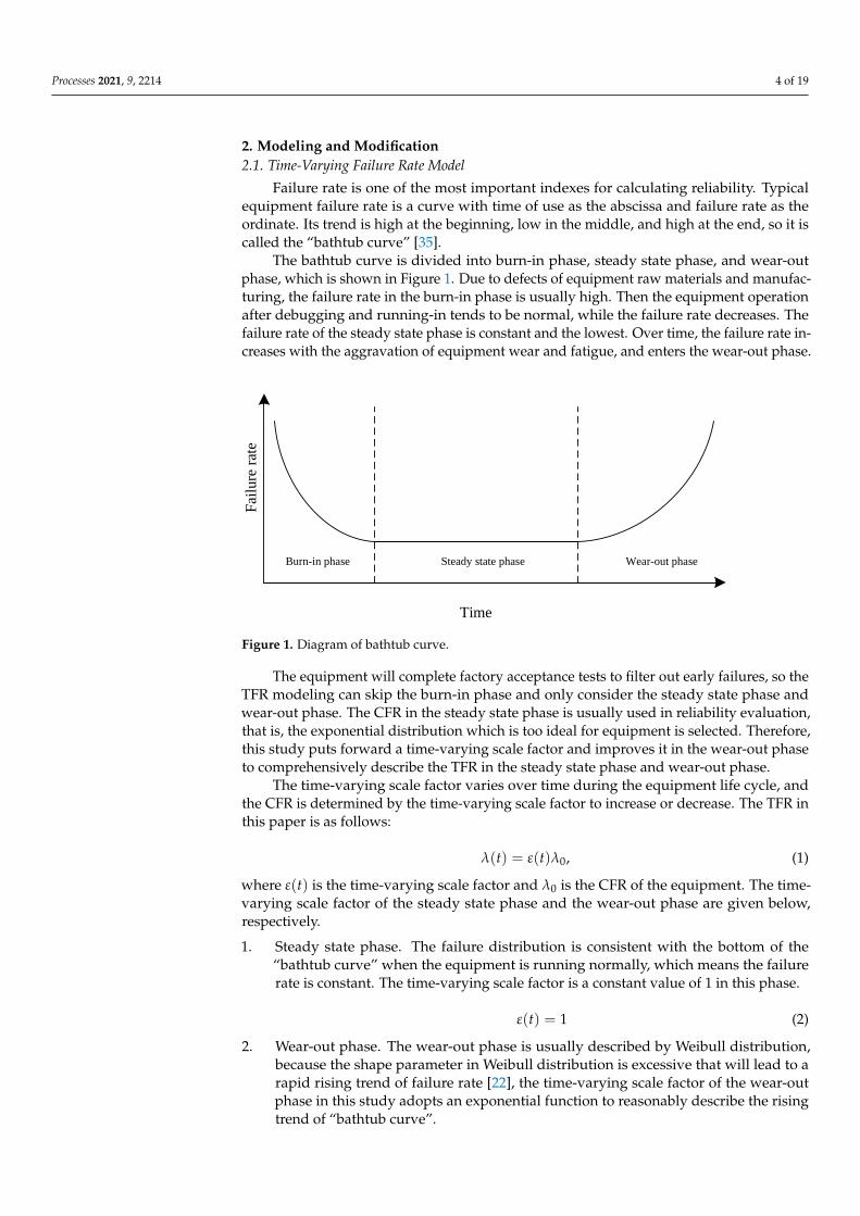
Failure rate is one of the most important indexes for calculating reliability. Typicalequipment failure rate is a curve with time of use as the abscissa and failure rate as theordinate. Its trend is high at the beginning, low in the middle, and high at the end, so it iscalled the “bathtub curve” [35].

The bathtub curve is divided into burn-in phase, steady state phase, and wear-outphase, which is shown in Figure 1. Due to defects of equipment raw materials and manufac-turing, the failure rate in the burn-in phase is usually high. Then the equipment operationafter debugging and running-in tends to be normal, while the failure rate decreases. Thefailure rate of the steady state phase is constant and the lowest. Over time, the failure rate in-creases with the aggravation of equipment wear and fatigue, and enters the wear-out phase.

Burn-in phase

Fai

lure

rat

e

Time

Steady state phase Wear-out phase

Figure 1. Diagram of bathtub curve.

The equipment will complete factory acceptance tests to filter out early failures, so theTFR modeling can skip the burn-in phase and only consider the steady state phase andwear-out phase. The CFR in the steady state phase is usually used in reliability evaluation,that is, the exponential distribution which is too ideal for equipment is selected. Therefore,this study puts forward a time-varying scale factor and improves it in the wear-out phaseto comprehensively describe the TFR in the steady state phase and wear-out phase.

The time-varying scale factor varies over time during the equipment life cycle, andthe CFR is determined by the time-varying scale factor to increase or decrease. The TFR inthis paper is as follows:

λ(t) = ε(t)λ0, (1)

where ε(t) is the time-varying scale factor and λ0 is the CFR of the equipment. The time-varying scale factor of the steady state phase and the wear-out phase are given below,respectively.

1. Steady state phase. The failure distribution is consistent with the bottom of the“bathtub curve” when the equipment is running normally, which means the failurerate is constant. The time-varying scale factor is a constant value of 1 in this phase.

ε(t) = 1 (2)

2. Wear-out phase. The wear-out phase is usually described by Weibull distribution,because the shape parameter in Weibull distribution is excessive that will lead to arapid rising trend of failure rate [22], the time-varying scale factor of the wear-outphase in this study adopts an exponential function to reasonably describe the risingtrend of “bathtub curve”.

Processes 2021, 9, 2214 5 of 19

ε(t) = eη(t−T), (3)

where η is the failure rate cumulated parameter of equipment, and T is the durationof the steady state phase. Combined with the previous equations, the TFR model ofthis paper is determined as:

λ(t) = ε(t)λ0 =

{λ0 t ≤ Teη(t−T)λ0 t > T

(4)

2.2. Statistical-Fuzzy Model of the Failure Rate Cumulated Parameter

There is a degree of uncertainty in the failure rate cumulated parameter obtainedeither by fitting failure data or by using expert experience. The fitting may suffer frommissing data and low precision, and expert experience is subjective. In this paper, theinterval value of the failure rate cumulated parameter is used instead of the single value,which can not only express the uncertainty of the parameter quantitatively, but also enablethe reliability analysis result to cover this uncertainty. Since the concept of the cut set infuzzy membership function is consistent with a range [34], this study uses the parameterestimation in mathematical statistics combined with expert experience to carry out intervalestimation for failure rate cumulated parameter. The Pseudo-Gaussian (PG) membershipfunction of the failure rate cumulated parameter is further obtained, and the statistical-fuzzy model of the failure rate cumulated parameter is established to directly reflect theuncertainty interval of the failure rate cumulated parameter.

The failure rate cumulated parameter η is estimated using the chi-square distributionat a given significant level α0.[

ηα0L , ηα0

U]=[χ2

1−α0/2(2r)/2Tr, χ2α0/2(2r + 2)/2Tr

](r = 1, 2, · · · , n− 1), (5)

η̄ = η0, (6)

where χ21−α0/2(2r) is the quantile when the integral from 0 to χ2

1−α0/2(2r) of chi-squaredistribution is α0/2 under the degree of freedom 2r, χ2

α0/2(2r + 2) is the quantile whenthe integral from χ2

α0/2(2r + 2) to ∞ is α0/2 under the degree of freedom 2r + 2. Tr is thestatistical time, and η0 is the expert experience value.

Considering the asymmetry when using the chi-square distribution, a PG membershipfunction of the failure rate cumulated parameter is established.

f (x, σ, c) =

exp

[− (x−c)2

σL2

]x ≤ c

exp[− (x−c)2

σR2

]x > c

, (7)

where x represents the failure rate cumulated parameter, and c is the expert experiencevalue of the failure rate cumulated parameter, σL and σR are the scale parameters of the leftand right parts of the PG membership function, respectively.

The degree of membership is similar to the concept of significant level, both of whichcan reflect subjective confidence degree. Therefore, the upper and lower bounds of thefailure rate cumulated parameter η in (5) correspond to the upper and lower boundaries atthe 1− α0-cut of the PG membership function.

exp[− (η

α0L −η0)

2

σL2

]= 1− α0

exp[− (η

α0U −η0)

2

σR2

]= 1− α0

(8)

Processes 2021, 9, 2214 6 of 19

σL and σR of the PG membership function of η can be estimated after the transforma-tion of (8). {

σL = −(ηα0L − η0)/

√− ln(1− α0)

σR = (ηα0U − η0)/

√− ln(1− α0)

(9)

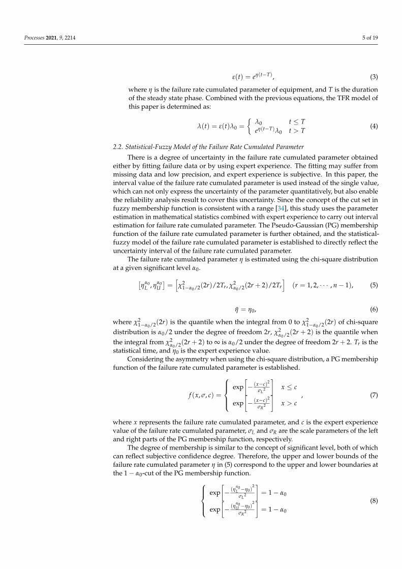
The PG membership function of the failure rate cumulated parameter can be obtainedby substituting (9) into (7), which is a convex function in the real number field as shown inFigure 2.

1

01 −

0

L

0

U

0

0(

,)

f

Figure 2. Diagram of the PG membership function for failure rate cumulated parameter.

Extending the PG membership function f (η, αi) to the general form as:

f (η, αi) =

exp

[(η−η0)

2 ln(1−αi)

(ηαiL −η0)

2

]η ≤ η0

exp[(η−η0)

2 ln(1−αi)

(ηαiU −η0)

2

]η > η0

, (10)

where 1− αi is an arbitrary cut set.

2.3. Modification of Time-Varying Failure Rate Model

Different failure rate cumulated parameter η corresponds to different trends of TFRcurves, and the time-varying scaling factor characterizing by the exponential functionincreases monotonically with η during wear-out phase, so

[η

αiL , η

αiU]

corresponds to a regionenclosed by innumerable TFR curves. The upper and lower boundaries of the regionare determined by the upper and lower boundaries of the interval, which intuitivelyreflects the degree of uncertainty contained in system reliability analysis. In order tomake the reliability analysis of the system with uncertainty have practical significance, theuncertainty of the failure rate cumulated parameter cannot exceed a certain range, and theupper and lower boundaries of the region enclosed by the failure rate curves should befocused on. Considering that the membership function can be used to describe the degreeto which the object belongs to a certain definition, this study proposes a new method tomodify the TFR model by using the statistical-fuzzy model of the failure rate cumulatedparameter. This method can more objectively and accurately specify the upper and lowerboundaries of the region enclosed by the modified failure rate curves.

Firstly, the upper and lower boundaries of[η

αiL , η

αiU]

and η0 are substituted into (4),respectively, and the corresponding TFR models are as follows:

λη

αiL(t) = ε

ηαiL(t)λ0 =

{λ0 t ≤ Teη

αiL (t−T)λ0 t > T

(11)

Processes 2021, 9, 2214 7 of 19

λη

αiU(t) = ε

ηαiU(t)λ0 =

{λ0 t ≤ Teη

αiU (t−T)λ0 t > T

(12)

λη0(t) = εη0(t)λ0 =

{λ0 t ≤ Teη0(t−T)λ0 t > T

(13)

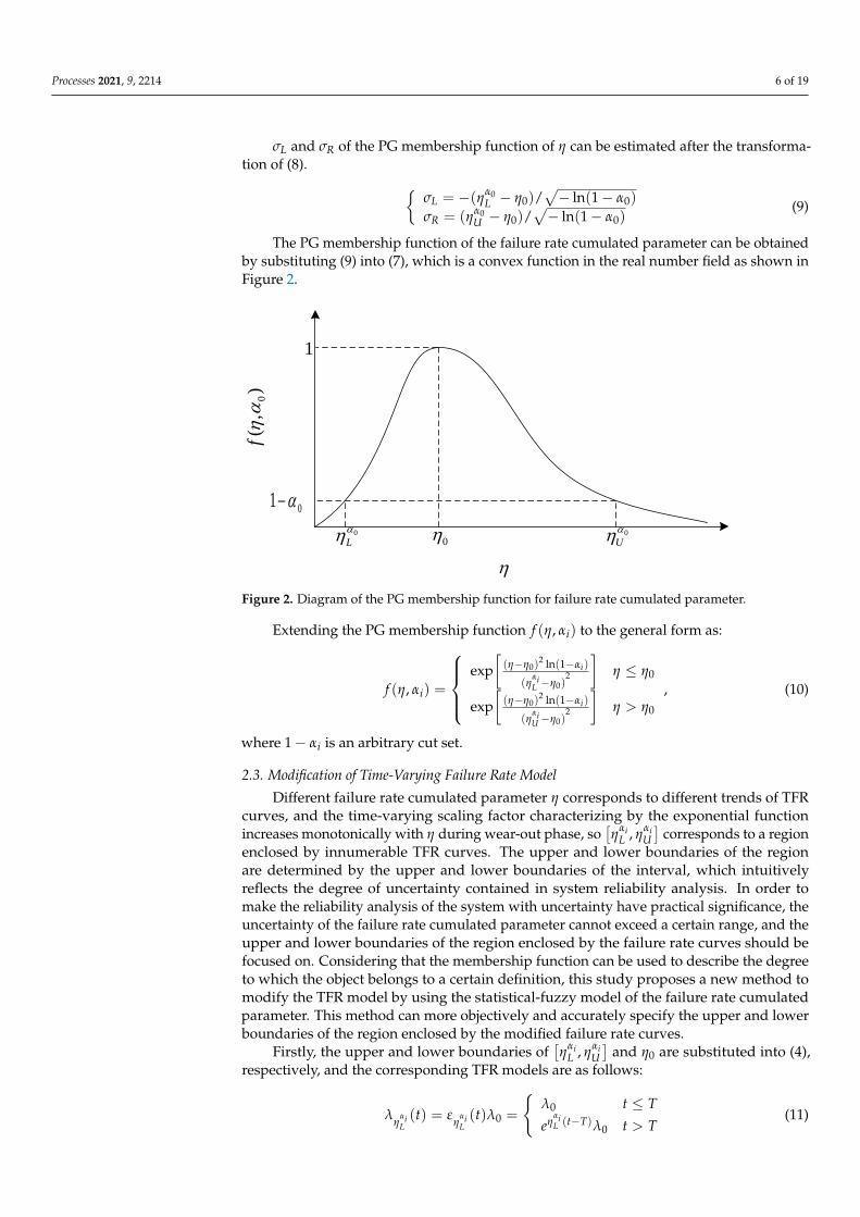
The TFR curve drawn from (11)–(13) is shown in Figure 3. It can be directly observedthat the failure rate curve corresponding to η

αiL rises the slowest, and the failure rate

curve corresponding to ηαiU rises the most rapidly. The failure rate curve corresponding

to η0 is sandwiched between the upper and lower boundary curves. The failure rateλ

ηαiL< λη0 < λ

ηαiU

at any same time point in the wear-out phase.

Time

( )t

0

iL

iU

t

0

Figure 3. Time-varying failure rate curves under different failure rate cumulated parameter.

To consider the confidence attached to η in the failure rate model objectively, theTFR model is modified using the statistical-fuzzy model of η. This method is only for thewear-out phase where parameter uncertainty exists, and the modified model is as follows:

λmo(t) = λ(t) · f (η, αi) = eη(t−T)λ0 · exp

[(η − η0)

2 ln(1− αi)

(ηαi − η0)2

](14)

The upper and lower boundaries of[η

αiL , η

αiU]

and η0 are substituted into (14), and thecorresponding modified TFR models are as follows:

λmo,ηαiL(t) =

{λ0 t ≤ T(1− αi)eη

αiL (t−T)λ0 t > T

(15)

λmo,ηαiU(t) =

{λ0 t ≤ T(1− αi)eη

αiU (t−T)λ0 t > T

(16)

λmo,η0(t) ={

λ0 t ≤ Teη0(t−T)λ0 t > T

(17)

When the TFR model is modified by the statistical-fuzzy model of η, the size order offailure rates λ

ηαiL

, λη0 and λη

αiU

at any same time point in the wear-out phase will change,

and the upper and lower boundaries of the region enclosed by TFR curves will also changesynchronously. The degree of change is discussed in Section 3.

Processes 2021, 9, 2214 8 of 19

3. The Existence Proof of Upper Boundary of Modified TFR Region3.1. The Upper Boundary Existence Theorem and Proof

The membership function of the failure rate cumulated parameter and the failure ratefunction of the wear-out phase both increase monotonically within the interval

[η

αiL , η0

].

From (14), it can be seen that the modified failure rate function λmo,ηαiL(t) < λmo,η0(t)

always holds. Comparing (15) and (16), it can be seen that the modified failure rate functionλmo,η

αiL(t) < λmo,η

αiU(t) always holds. This study focuses on the TFR model modified by the

PG membership function on the right half.

λmo(t) = eη(t−T)λ0 · exp

[(η − η0)

2 ln(1− αi)

(ηαiU − η0)

2

](18)

The TFR function is shifted T units to the left ignoring the steady state phase, and themodified TFR model is simplified as:

λmo(t) = eηtλ0 · exp

[(η − η0)

2 ln(1− αi)

(ηαiU − η0)

2

](19)

Theorem 1. The upper boundary existence theorem.

Assuming that parameters t, αi, η0, λ0 are given, there is a definite upper bound-ary of the region bounded by λmo(t) under the domain

[ηα0

L , ηα0U]

of η, if and only if

η = min{

ηαiU , η0 − (ηαi

U − η0)2t/2 ln(1− αi)

}.

Proof of Theorem 1. Given that t, αi, η0, λ0, so ηαiU is also a definite value, then only η is

the independent variable in λmo(t). Rewrite λmo(t) as λmo(η), and take the derivative of ηin λmo(η).

dλmo(η)

dη= λ0eηt · exp

[(η − η0)

2 ln(1− αi)

(ηαiU − η0)

2

]·[

t +2(η − η0) ln(1− αi)

(ηαiU − η0)

2

](20)

Let (20) be rewritten as:

dλmo(η)

dη= g(η) · h(η), (21)

where:

g(η) = λ0eηt · exp

[(η − η0)

2 ln(1− αi)

(ηαiU − η0)

2

](22)

h(η) = t +2(η − η0) ln(1− αi)

(ηαiU − η0)

2 (23)

According to the properties of failure rate and the exponential function, λ0 > 0,

eηt > 0, exp[(η−η0)

2 ln(1−αi)

(ηαiU −η0)

2

]> 0 always hold, therefore g(η) > 0 always holds. The

following focuses on h(η).

h(η) = Kη + R (24)

Combining (23) and (24), the following can be obtained:

K =2 ln(1− αi)

(ηαiU − η0)

2 (25)

Processes 2021, 9, 2214 9 of 19

R = t− 2η0 ln(1− αi)

(ηαiU − η0)

2 (26)

αi ∈ [0, 1], t > 0, η0 > 0 is known, so K < 0, R > 0 always hold. It can be seen thath(η) is a straight line decreasing monotonically that intersects the positive vertical axis.Suppose the intersection point of h(η) and the horizontal axis is η′, it follows that η′ > 0.Furthermore, it is known that: {

h(η) > 0 η < η′

h(η) ≤ 0 η ≥ η′(27)

Combining (21), (22), and (27) can be obtained:dλmo(η)

dη > 0 η < η′

dλmo(η)dη ≤ 0 η ≥ η′

(28)

Therefore, λmo(η) increases first and then decreases progressively, and there must be alocal maximum value in the real number field. Given h(η′) = 0, the local maximum point is:

η′ = η0 −(ηαi

U − η0)2t

2 ln(1− αi)> η0 (29)

Given η ∈[ηα0

L , ηα0U], to further obtain the maximum point of λmo(η), compare the

size of η′ and ηαiU by subtracting the two:

η′ − ηαiU =

(η0 − ηαiU )[2 ln(1− αi)− (η0 − η

αiU )t]

2 ln(1− αi), (30)

where η0 − ηαiU < 0, 2 ln(1− αi) < 0.

According to (30), comparing the size of η′ and ηαiU means discussing the sign of

2 ln(1− αi)− (η0 − ηαiU )t.{

ηαiU > η0 − 2 ln(1− αi)/t η′ > η

αiU

ηαiU < η0 − 2 ln(1− αi)/t η′ < η

αiU

(31)

Substitute ηαiU = χ2

α0/2(2r + 2)/2Tr into (31).{χ2

α0/2(2r + 2) > 2Trη0 − 4Tr ln(1− αi)/t η′ > ηαiU

χ2α0/2(2r + 2) < 2Trη0 − 4Tr ln(1− αi)/t η′ < η

αiU

, (32)

where χ2α0/2(2r + 2) is the quantile of the chi-square distribution table, which can be

obtained by referring to the table.Equation (32) shows that there are mathematical conditions to determine the size of η′

and ηαiU . Since λmo(η) increases first and then decreases, the maximum point in domain

η ∈[ηα0

L , ηα0U]

is ηαiU when η′ > η

αiU , and the maximum point is η′ when η′ < η

αiU .

To sum up: Assuming that parameters t, αi, η0, λ0 are given, there is a definite upperboundary of the region bounded by λmo(t) under the domain

[ηα0

L , ηα0U]

of η, if and only if

η = min{

ηαiU , η0 − (ηαi

U − η0)2t/2 ln(1− αi)

}. Theorem proving completed.

3.2. Numerical Example

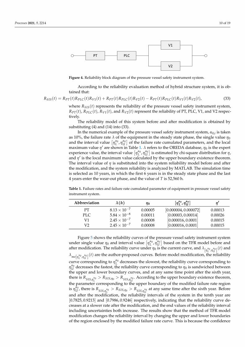
A long-running pressure vessel safety instrument system [36] is composed of pressuretransmitter (PT), programmable logic controller (PLC), valve 1 (V1) and valve 2 (V2). ThePT measures the pressure in the vessel and feeds back to the PLC, and the PLC will shutdown V1 and V2 when the pressure exceeds the warning value. Figure 4 is reliability blockdiagram of the system, in which V1 and V2 are connected in parallel and then connected inseries with PT and PLC.

Processes 2021, 9, 2214 10 of 19

PT

V1

V2

PLC

Figure 4. Reliability block diagram of the pressure vessel safety instrument system.

According to the reliability evaluation method of hybrid structure system, it is ob-tained that:

RSIS(t) = RPT(t)RPLC(t)RV1(t) + RPT(t)RPLC(t)RV2(t)− RPT(t)RPLC(t)RV1(t)RV2(t), (33)

where RSIS(t) represents the reliability of the pressure vessel safety instrument system,RPT(t), RPLC(t), RV1(t), and RV2(t) represent the reliability of PT, PLC, V1, and V2 respec-tively.

The reliability model of this system before and after modification is obtained bysubstituting (4) and (14) into (33).

In the numerical example of the pressure vessel safety instrument system, α0,i is takenas 10%, the failure rate λ of the equipment in the steady state phase, the single value η0and the interval value

[ηα0

L , ηα0U]

of the failure rate cumulated parameters, and the localmaximum value η′ are shown in Table 1. λ refers to the OREDA database, η0 is the expertexperience value, the interval value

[ηα0

L , ηα0U]

is estimated by chi-square distribution for η,and η′ is the local maximum value calculated by the upper boundary existence theorem.The interval value of η is substituted into the system reliability model before and afterthe modification, and the system reliability is analyzed by MATLAB. The simulation timeis selected as 10 years, in which the first 6 years is in the steady state phase and the last4 years enter the wear-out phase, and the value of T is 52,560 h.

Table 1. Failure rates and failure rate cumulated parameter of equipment in pressure vessel safetyinstrument system.

Abbreviation λ(h) η0 [ηα0L , ηα0

U ] η′

PT 8.13× 10−7 0.00005 [0.000004, 0.000072] 0.00013PLC 5.84× 10−8 0.00011 [0.00003, 0.00014] 0.00026V1 2.45× 10−7 0.00008 [0.000016, 0.0001] 0.00015V2 2.45× 10−7 0.00008 [0.000016, 0.0001] 0.00015

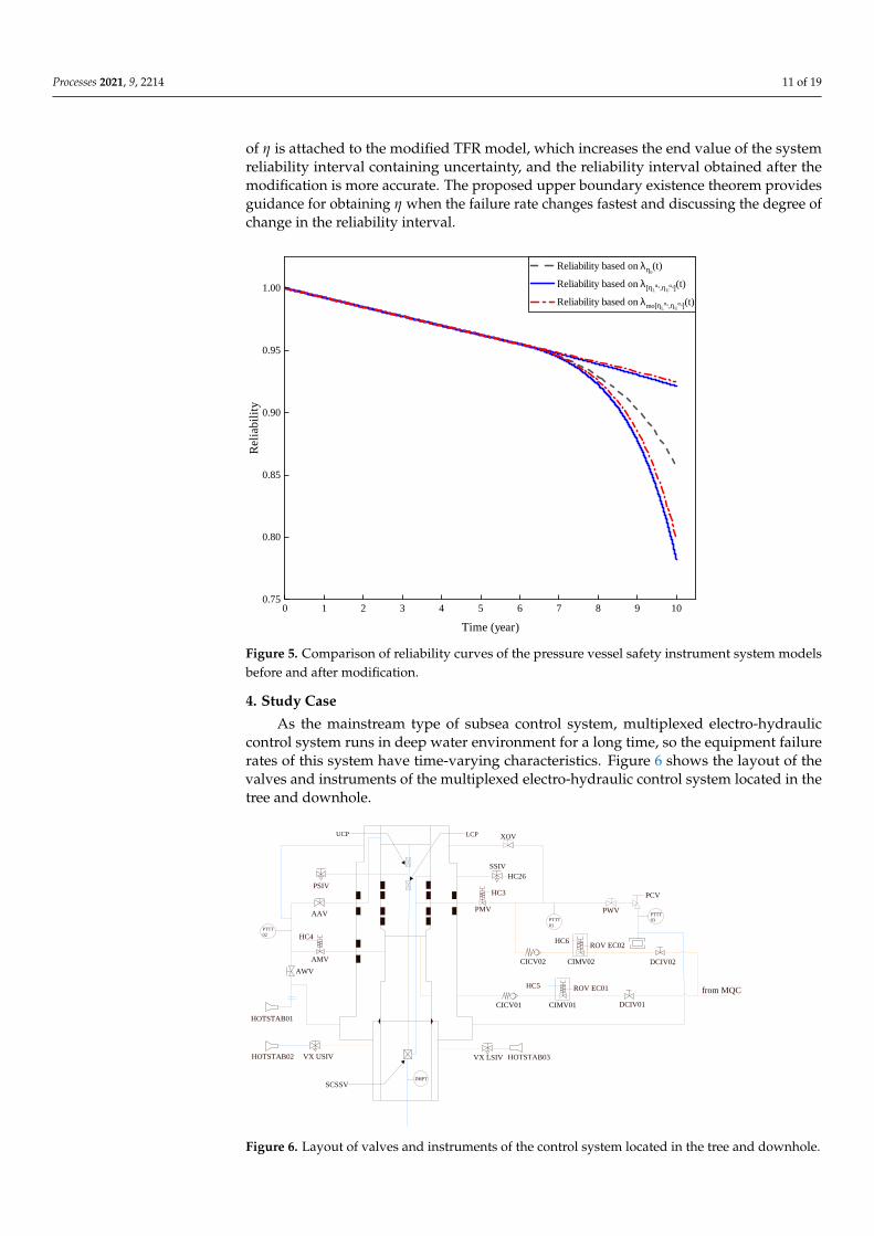
Figure 5 shows the reliability curves of the pressure vessel safety instrument systemunder single value η0 and interval value

[ηα0

L , ηα0U]

based on the TFR model before andafter modification. The reliability curve under η0 is the current curve, and λ[η

α0L ,η

α0U ](t) and

λmo[ηα0L ,η

α0U ](t) are the author-proposed curves. Before model modification, the reliability

curve corresponding to ηα0L decreases the slowest, the reliability curve corresponding to

ηα0U decreases the fastest, the reliability curve corresponding to η0 is sandwiched between

the upper and lower boundary curves, and at any same time point after the sixth year,there is RSIS,η

α0L

> RSIS,η0 > RSIS,ηα0U

. According to the upper boundary existence theorem,the parameter corresponding to the upper boundary of the modified failure rate regionis ηα0

U , there is RSIS,ηα0L

> RSIS,η0 > RSIS,ηα0U

at any same time after the sixth year. Beforeand after the modification, the reliability intervals of the system in the tenth year are[0.7825, 0.9213] and [0.7986, 0.9246] respectively, indicating that the reliability curve de-creases at a slower rate after the modification, and the end values of the reliability intervalincluding uncertainties both increase. The results show that the method of TFR modelmodification changes the reliability interval by changing the upper and lower boundariesof the region enclosed by the modified failure rate curve. This is because the confidence

Processes 2021, 9, 2214 11 of 19

of η is attached to the modified TFR model, which increases the end value of the systemreliability interval containing uncertainty, and the reliability interval obtained after themodification is more accurate. The proposed upper boundary existence theorem providesguidance for obtaining η when the failure rate changes fastest and discussing the degree ofchange in the reliability interval.

0 1 2 3 4 5 6 7 8 9 1 00 . 7 5

0 . 8 0

0 . 8 5

0 . 9 0

0 . 9 5

1 . 0 0 R e l i a b i l i t y b a s e d o n λη0 ( t ) R e l i a b i l i t y b a s e d o n λ[ηL α 0 , ηU α 0 ]( t ) R e l i a b i l i t y b a s e d o n λ m o [ηL α 0 , ηU α 0 ]( t )

Reliab

ility

T i m e ( y e a r )Figure 5. Comparison of reliability curves of the pressure vessel safety instrument system modelsbefore and after modification.

4. Study Case

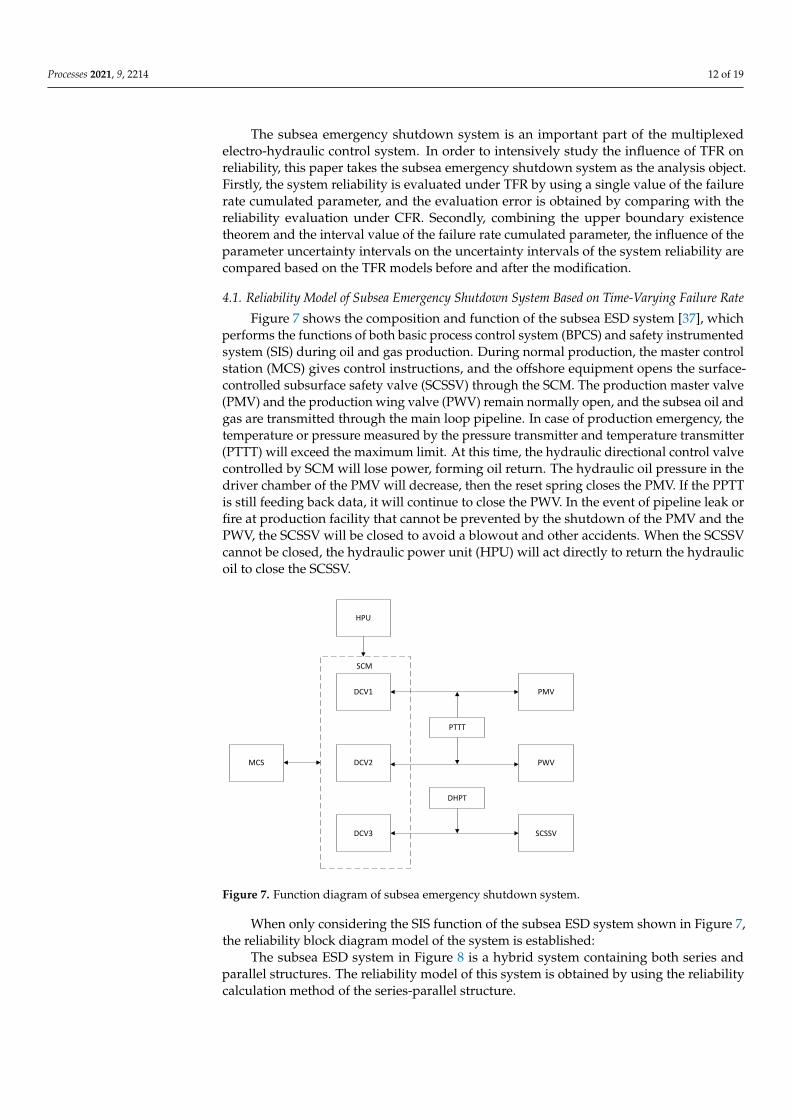
As the mainstream type of subsea control system, multiplexed electro-hydrauliccontrol system runs in deep water environment for a long time, so the equipment failurerates of this system have time-varying characteristics. Figure 6 shows the layout of thevalves and instruments of the multiplexed electro-hydraulic control system located in thetree and downhole.

PMV PWV

AMV

AAV

PTTT

02

XOV

SSIV

SCSSV

PCV

DCIV02

DCIV01CIMV01CICV01

CIMV02CICV02

VX LSIV

HC4

HC3

HC5

HC26

HC6ROV EC02

ROV EC01

LCP

VX USIV

from MQC

HOTSTAB01

HOTSTAB02 HOTSTAB03

UCP

PSIV

AWV

UCP

PSIV

HC26

PTTT

01

PTTT

03

DHPT

Figure 6. Layout of valves and instruments of the control system located in the tree and downhole.

Processes 2021, 9, 2214 12 of 19

The subsea emergency shutdown system is an important part of the multiplexedelectro-hydraulic control system. In order to intensively study the influence of TFR onreliability, this paper takes the subsea emergency shutdown system as the analysis object.Firstly, the system reliability is evaluated under TFR by using a single value of the failurerate cumulated parameter, and the evaluation error is obtained by comparing with thereliability evaluation under CFR. Secondly, combining the upper boundary existencetheorem and the interval value of the failure rate cumulated parameter, the influence of theparameter uncertainty intervals on the uncertainty intervals of the system reliability arecompared based on the TFR models before and after the modification.

4.1. Reliability Model of Subsea Emergency Shutdown System Based on Time-Varying Failure Rate

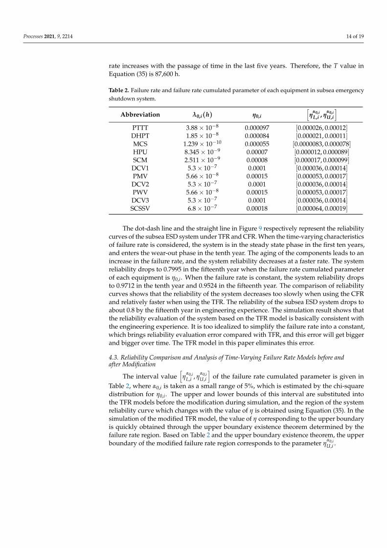
Figure 7 shows the composition and function of the subsea ESD system [37], whichperforms the functions of both basic process control system (BPCS) and safety instrumentedsystem (SIS) during oil and gas production. During normal production, the master controlstation (MCS) gives control instructions, and the offshore equipment opens the surface-controlled subsurface safety valve (SCSSV) through the SCM. The production master valve(PMV) and the production wing valve (PWV) remain normally open, and the subsea oil andgas are transmitted through the main loop pipeline. In case of production emergency, thetemperature or pressure measured by the pressure transmitter and temperature transmitter(PTTT) will exceed the maximum limit. At this time, the hydraulic directional control valvecontrolled by SCM will lose power, forming oil return. The hydraulic oil pressure in thedriver chamber of the PMV will decrease, then the reset spring closes the PMV. If the PPTTis still feeding back data, it will continue to close the PWV. In the event of pipeline leak orfire at production facility that cannot be prevented by the shutdown of the PMV and thePWV, the SCSSV will be closed to avoid a blowout and other accidents. When the SCSSVcannot be closed, the hydraulic power unit (HPU) will act directly to return the hydraulicoil to close the SCSSV.

MCS DCV2

PMV

PWV

SCSSVDCV3

DCV1

PTTT

DHPT

HPU

SCM

Figure 7. Function diagram of subsea emergency shutdown system.

When only considering the SIS function of the subsea ESD system shown in Figure 7,the reliability block diagram model of the system is established:

The subsea ESD system in Figure 8 is a hybrid system containing both series andparallel structures. The reliability model of this system is obtained by using the reliabilitycalculation method of the series-parallel structure.

Processes 2021, 9, 2214 13 of 19

Rsys = [(R1 + R2 − R1R2)R3 + R4 − (R1 + R2 − R1R2)R3R4] · R5 · [R6R7 + R8R9− R6R7R8R9 + R10R11 − (R6R7 + R8R9 − R6R7R8R9)R10R11)]

, (34)

where Rsys represents the reliability of the subsea ESD system, and Ri represents thereliability of the equipment PTTT, DHPT, MCS, HPU, SCM, DCV1, PMV, DCV2, PWV,DCV3, and SCSSV of the system in turn.

MCS

HPU

DCV1 PMV

DCV2 PWV

DCV3 SCSSV

PTTT

DHPT

SCM

Figure 8. Reliability block diagram of subsea emergency shutdown system.

1. Equipment reliability model based on time-varying failure rate model before modifica-tion. The TFR model for each equipment of the subsea ESD system before modificationis obtained using (4), then the reliability model of the equipment is as follows:

Ri(t) =

e−λ0,it t ≤ T

exp(

λ0,i−λ0,ieη0,i(t−T)

η0,i

)+e−λ0,iT − 1 t > T

, (35)

When i = 1, 2, · · · , 11, Ri, λ0,i and η0,i, respectively, represent the reliability, failurerate in the steady state phase and the single value of failure rate cumulated parameterof the equipment PTTT, DHPT, MCS, HPU, SCM, DCV1, PMV, DCV2, PWV, DCV3,and SCSSV in this system.

2. Equipment reliability model based on time-varying failure rate model after modifica-tion. The modified TFR model (14)–(17), for a given α0,i, when ηi < η0,i,

Ri,mo(t) =

e−λ0,it t ≤ T

exp

(exp

((ηi−η0,i)

2 ln(1−α0,i)

(ηα0,iL,i −η0,i)

2

)· λ0,i−λ0,ieηi(t−T)

ηi

)+e−λ0,iT − 1 t > T

(36)

When ηi > η0,i,

Ri,mo(t) =

e−λ0,it t ≤ T

exp

(exp

((ηi−η0,i)

2 ln(1−α0,i)

(ηα0,iU,i −η0,i)

2

)· λ0,i−λ0,ieηi(t−T)

ηi

)+e−λ0,iT − 1 t > T

(37)

Substituting the reliability model before and after modification of the equipment(35)–(37) into (34), the reliability models of the system based on the TFR model beforeand after modification are obtained.

4.2. Reliability Comparison and Analysis Based on Time-Varying Failure Rate and ConstantFailure Rate Models

As shown in Table 2, the failure rate of each equipment λ0,i(h) in the subsea ESDsystem in the steady state phase refers to the OREDA, and the failure rate cumulatedparameter is the expert experience value. The simulation is carried out in MATLAB, andthe simulation time is 15 years, which is 131,400 hours. When considering the time-varyingcharacteristics of failure rate, the first ten years is the steady state phase, and the failure

Processes 2021, 9, 2214 14 of 19

rate increases with the passage of time in the last five years. Therefore, the T value inEquation (35) is 87,600 h.

Table 2. Failure rate and failure rate cumulated parameter of each equipment in subsea emergencyshutdown system.

Abbreviation λ0,i(h) η0,i

[η

α0,iL,i , η

α0,iU,i

]PTTT 3.88× 10−8 0.000097 [0.000026, 0.00012]DHPT 1.85× 10−8 0.000084 [0.000021, 0.00011]MCS 1.239× 10−10 0.000055 [0.0000083, 0.000078]HPU 8.345× 10−9 0.00007 [0.000012, 0.000089]SCM 2.511× 10−9 0.00008 [0.000017, 0.000099]

DCV1 5.3× 10−7 0.0001 [0.000036, 0.00014]PMV 5.66× 10−8 0.00015 [0.000053, 0.00017]DCV2 5.3× 10−7 0.0001 [0.000036, 0.00014]PWV 5.66× 10−8 0.00015 [0.000053, 0.00017]DCV3 5.3× 10−7 0.0001 [0.000036, 0.00014]SCSSV 6.8× 10−7 0.00018 [0.000064, 0.00019]

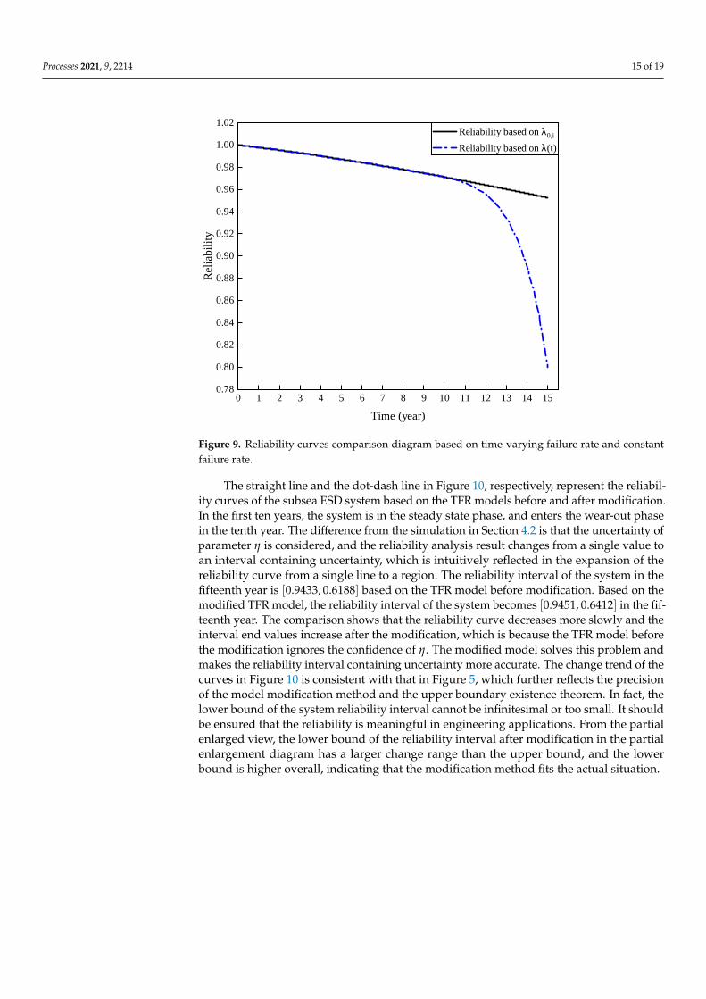
The dot-dash line and the straight line in Figure 9 respectively represent the reliabilitycurves of the subsea ESD system under TFR and CFR. When the time-varying characteristicsof failure rate is considered, the system is in the steady state phase in the first ten years,and enters the wear-out phase in the tenth year. The aging of the components leads to anincrease in the failure rate, and the system reliability decreases at a faster rate. The systemreliability drops to 0.7995 in the fifteenth year when the failure rate cumulated parameterof each equipment is η0,i. When the failure rate is constant, the system reliability dropsto 0.9712 in the tenth year and 0.9524 in the fifteenth year. The comparison of reliabilitycurves shows that the reliability of the system decreases too slowly when using the CFRand relatively faster when using the TFR. The reliability of the subsea ESD system drops toabout 0.8 by the fifteenth year in engineering experience. The simulation result shows thatthe reliability evaluation of the system based on the TFR model is basically consistent withthe engineering experience. It is too idealized to simplify the failure rate into a constant,which brings reliability evaluation error compared with TFR, and this error will get biggerand bigger over time. The TFR model in this paper eliminates this error.

4.3. Reliability Comparison and Analysis of Time-Varying Failure Rate Models before andafter Modification

The interval value[η

α0,iL,i , η

α0,iU,i

]of the failure rate cumulated parameter is given in

Table 2, where α0,i is taken as a small range of 5%, which is estimated by the chi-squaredistribution for η0,i. The upper and lower bounds of this interval are substituted intothe TFR models before the modification during simulation, and the region of the systemreliability curve which changes with the value of η is obtained using Equation (35). In thesimulation of the modified TFR model, the value of η corresponding to the upper boundaryis quickly obtained through the upper boundary existence theorem determined by thefailure rate region. Based on Table 2 and the upper boundary existence theorem, the upperboundary of the modified failure rate region corresponds to the parameter η

α0,iU,i .

Processes 2021, 9, 2214 15 of 19

0 1 2 3 4 5 6 7 8 9 1 0 1 1 1 2 1 3 1 4 1 50 . 7 80 . 8 00 . 8 20 . 8 40 . 8 60 . 8 80 . 9 00 . 9 20 . 9 40 . 9 60 . 9 81 . 0 01 . 0 2 R e l i a b i l i t y b a s e d o n λ 0 , i

R e l i a b i l i t y b a s e d o n λ ( t )

Reliab

ility

T i m e ( y e a r )Figure 9. Reliability curves comparison diagram based on time-varying failure rate and constantfailure rate.

The straight line and the dot-dash line in Figure 10, respectively, represent the reliabil-ity curves of the subsea ESD system based on the TFR models before and after modification.In the first ten years, the system is in the steady state phase, and enters the wear-out phasein the tenth year. The difference from the simulation in Section 4.2 is that the uncertainty ofparameter η is considered, and the reliability analysis result changes from a single value toan interval containing uncertainty, which is intuitively reflected in the expansion of thereliability curve from a single line to a region. The reliability interval of the system in thefifteenth year is [0.9433, 0.6188] based on the TFR model before modification. Based on themodified TFR model, the reliability interval of the system becomes [0.9451, 0.6412] in the fif-teenth year. The comparison shows that the reliability curve decreases more slowly and theinterval end values increase after the modification, which is because the TFR model beforethe modification ignores the confidence of η. The modified model solves this problem andmakes the reliability interval containing uncertainty more accurate. The change trend of thecurves in Figure 10 is consistent with that in Figure 5, which further reflects the precisionof the model modification method and the upper boundary existence theorem. In fact, thelower bound of the system reliability interval cannot be infinitesimal or too small. It shouldbe ensured that the reliability is meaningful in engineering applications. From the partialenlarged view, the lower bound of the reliability interval after modification in the partialenlargement diagram has a larger change range than the upper bound, and the lowerbound is higher overall, indicating that the modification method fits the actual situation.

Processes 2021, 9, 2214 16 of 19

0 1 2 3 4 5 6 7 8 9 1 0 1 1 1 2 1 3 1 4 1 50 . 6 0

0 . 6 5

0 . 7 0

0 . 7 5

0 . 8 0

0 . 8 5

0 . 9 0

0 . 9 5

1 . 0 0

1 . 0 5 R e l i a b i l i t y b a s e d o n λ ( t ) R e l i a b i l i t y b a s e d o n λ m o ( t )

Reliab

ility

T i m e ( y e a r )Figure 10. Reliability curves comparison diagram based on time-varying failure rate models beforeand after modification.

5. Conclusions

The failure rate of most equipment varies with time in long-term operation. In orderto solve the problem of reliability evaluation error caused by constant failure rate, a newtime-varying failure rate model is established after comprehensively considering the time-varying characteristics of the failure rate in the steady state phase and wear-out phase.The time-varying scale factor in the model included the failure rate cumulated parametersthat influenced the curve trend. Due to the uncertainty of the failure rate cumulatedparameter, a statistical-fuzzy model is established based on the interval of the failure ratecumulated parameter estimated by the parameter estimation combined with statistics andfuzzy knowledge. In addition, the TFR model is modified by using statistical-fuzzy model,which covers the confidence of the failure rate cumulated parameter, and changes the upperand lower boundaries of the region enclosed by the failure rate curves. To further explorethe range of boundary variation, the upper boundary existence theorem for the failure rateregion is proposed and demonstrated, so as to obtain the failure rate cumulated parameterwhen the failure rate changes fastest, and the theorem is applied to numerical example.

In this paper, the subsea emergency shutdown system which has been in marineenvironment for a long time is selected as the research object, and the reliability model isestablished by using time-varying failure rate model and system reliability block diagram.When the failure rate cumulated parameter is a single value, the reliability of the systemsunder time-varying failure rate and constant failure rate are compared and analyzed. Whenthe failure rate cumulated parameter is an interval, combined with the upper boundaryexistence theorem for the failure rate region, the system reliability based on the time-varying failure rate models before and after the modification are compared and analyzed.The following conclusions are drawn.

1. Compared with the constant failure rate, the system reliability with the time-varyingfailure rate decreases faster and reaches 0.7995 in the fifteenth year. The reliability inthe fifteenth year in engineering experience is about 0.8, so the time-varying failurerate model proposed in this paper is consistent with the actual situation and caneliminate the reliability evaluation error caused by the constant failure rate.

Processes 2021, 9, 2214 17 of 19

2. Compared with the model before the modification, the modified time-varying failurerate model has the confidence of η attached, which increases the end value of thesystem reliability interval containing uncertainty, and the reliability interval obtainedafter the modification is more accurate and realistic.

In practical engineering, the system requires equipment maintenance based on relia-bility evaluation, so the reliability interval obtained from the modified failure rate modelproposed in this study can theoretically provide data support for maintenance strategy andmake it more flexible, and this work will be completed in the future.

Author Contributions: Conceptualization, X.Z. and X.Y.; methodology, X.Y.; software, X.Y.; valida-tion, X.Z., X.Y. and Y.Y.; formal analysis, Y.Y.; investigation, X.Y.; resources, F.Y.; data curation, F.Y. andC.Z.; writing—original draft preparation, X.Y.; writing—review and editing, X.Z.; visualization, X.Y.;supervision, Y.Y.; project administration, X.Z.; funding acquisition, X.Z., F.Y. and C.Z. All authorshave read and agreed to the published version of the manuscript.

Funding: This work is supported by National High-tech Ships from Ministry of Industry andInformation Technology: Research on Integral Reliability Analysis Technology of Subsea ControlSystem (2018GXB01-03-004), Science Foundation of China University of Petroleum, Beijing (No.2462020YXZZ023).

Institutional Review Board Statement: Not applicable.

Informed Consent Statement: Not applicable.

Data Availability Statement: Not applicable.

Conflicts of Interest: The authors declare no conflict of intrerst.

Abbreviations

ESD Emergency shutdownCFR Constant failure rateTFR Time-varying failure rateOREDA Offshore and onshore reliability dataSCM Subsea control modulePG Pseudo-gaussianPT Pressure transmitterPLC Programmable logic controllerV1 Valve 1V2 Valve 2BPCS Basic process control systemSIS Safety instrumented systemMCS Master control stationHPU Hydraulic power unitPTTT Pressure transmitter and temperature transmitterDHPT Downhole pressure and temperature transmitterPMV Production master valvePWV Production wing valveSCSSV Surface controlled subsurface safety valveDCV1 Directional control valve 1DCV2 Directional control valve 2DCV3 Directional control valve 3

References1. Zhang, Y.; Tang, W.; Du, J. Development of subsea production system and its control system. In Proceedings of the 2017 4th

International Conference on Information, Cybernetics and Computational Social Systems (ICCSS), Dalian, China, 24–26 July 2017;pp. 117–122. [CrossRef]

2. lyalla, I.; Arulliah, E.; Innes, D. A critical analysis of open protocol for subsea production controls system communication. InProceedings of the OCEANS 2017, Aberdeen, UK, 19–22 June 2017; pp. 1–7. [CrossRef]

Processes 2021, 9, 2214 18 of 19

3. Bai, Y.; Bai, Q. (Eds.) 7—Subsea Control. In Subsea Engineering Handbook, 2nd ed.; Gulf Professional Publishing: Boston, MA, USA,2019; pp. 173–202. [CrossRef]

4. Hua, Y.; Kecheng, S.; Xin, D.; Chao, Y.; Yuanlong, Y. Adaptability Analysis of SubseaOil and Gas Control System in Bohai SeaRegion. Mech. Electr. Eng. Technol. 2021, 50, 60–63, 137.

5. Yangfeng, F.; Guochu, C. Application of subsea electro-hydraulic control system in deepwater gas field project. China Pet. Chem.Stand. Qual. 2020, 40, 125–126.

6. Lu, W.; Weizhenq, A. Comparison and Analysis of Subsea Production Control System. Petrochem. Ind. Technol. 2018, 25, 17–19.7. Nolan, D.P. (Ed.) Chapter 11—Emergency Shutdown. In Handbook of Fire and Explosion Protection Engineering Principles for Oil,

Gas, Chemical, and Related Facilities, 4th ed.; Gulf Professional Publishing: Waltham, MA, USA, 2019; pp. 215–225. [CrossRef]8. Wang, X.; Jia, P.; Lizhang, H.; Wang, L.; Yun, F.; Wang, H. Reliability and Safety Modelling of the Electrical Control System of the

Subsea Control Module Based on Markov and Multiple Beta Factor Model. IEEE Access 2019, 7, 6194–6208. [CrossRef]9. Pang, N.; Jia, P.; Wang, L.; Yun, F.; Wang, G.; Wang, X.; Shi, L. Dynamic Bayesian network-based reliability and safety assessment

of the subsea Christmas tree. Process. Saf. Environ. Prot. 2021, 145, 435–446. [CrossRef]10. Bae, J.H.; Shin, S.C.; Park, B.C.; Kim, S.Y. Design Optimization of ESD (Emergency ShutDown) System for Offshore Process Based

on Reliability Analysis. MATEC Web Conf. 2016, 52, 10. [CrossRef]11. Signorini, G.; Rigoni, E.; Rodrigues, M. Reliability Analysis Methodology for Oil and Gas Assets: Case Study of Subsea Control

Module Operating in Deep Water Basin at Brazilian Pre-Salt. In Proceedings of the 2020 International Petroleum TechnologyConference (IPTC), Dhahran, Saudi Arabia, 13–15 January 2020. [CrossRef]

12. Ismagilov, F.; Vavilov, V.; Karimov, R.; Yushkova, O.; Timofeev, A. Combined Method of Technical Analysis to Optimize theAviation Electromechanical Systems Reliability Indicators. In Proceedings of the 2021 28th International Workshop on ElectricDrives: Improving Reliability of Electric Drives (IWED), Moscow, Russia, 27–29 January 2021; pp. 1–4. [CrossRef]

13. Tang, Q.; Shu, X.; Zhu, G.; Wang, J.; Yang, H. Reliability Study of BEV Powertrain System and Its Components—A Case Study.Processes 2021, 9, 762. [CrossRef]

14. Tawfiq, A.A.E.; El-Raouf, M.O.A.; Mosaad, M.I.; Gawad, A.F.A.; Farahat, M.A.E. Optimal Reliability Study of Grid-Connected PVSystems Using Evolutionary Computing Techniques. IEEE Access 2021, 9, 42125–42139. [CrossRef]

15. Hassett, T.; Dietrich, D.; Szidarovszky, F. Time-varying failure rates in the availability and reliability analysis of repairablesystems. IEEE Trans. Reliab. 1995, 44, 155–160. [CrossRef]

16. Retterath, B.; Venkata, S.; Chowdhury, A. Impact of time-varying failure rates on distribution reliability. In Proceedings ofthe 2004 International Conference on Probabilistic Methods Applied to Power Systems, Ames, IA, USA, 12–16 September 2004;pp. 953–958. [CrossRef]

17. Wang, R.; Xue, A.; Huang, S.; Cao, X.; Shao, Z.; Luo, Y. On the estimation of time-varying failure rate to the protectiondevices based on failure pattern. In Proceedings of the 2011 4th International Conference on Electric Utility Deregulation andRestructuring and Power Technologies (DRPT), Weihai, China, 6–9 July 2011; pp. 902–905. [CrossRef]

18. Abunima, H.; Teh, J. Reliability Modeling of PV Systems Based on Time-Varying Failure Rates. IEEE Access 2020, 8, 14367–14376.[CrossRef]

19. Zhang, Q.; Wang, X.; Du, W.; Zhang, H.; Li, X. Reliability Model of Submarine Cable Based on Time-varying Failure Rate. InProceedings of the 2019 IEEE 8th International Conference on Advanced Power System Automation and Protection (APAP).Xi’an, China, 21–24 October 2019; pp. 711–715. [CrossRef]

20. Li, Q.; Wang, Z.; Zhao, H.; Liu, H.; Tian, L.; Zhang, X.; Qiu, J.; Xue, C.; Zhang, X. Research on Prediction Model of InsulationFailure Rate of Power Transformer Considering Real-time Aging State. In Proceedings of the 2019 IEEE 3rd Conference on EnergyInternet and Energy System Integration (EI2), Changsha, China, 8–10 November 2019; pp. 800–805. [CrossRef]

21. Jian, L.; Feng, G.; Ming, Z.; Liuning, C.; Weiyao, L. Research on Optimal Inspection Strategy for Overhead Transmission LineBased on Smart Grid. Procedia Comput. Sci. 2018, 130, 1134–1139. [CrossRef]

22. Liu, H.; Wang, Z.; Han, M. Reliability Analysis of Solenoid Valve Power Supply Based on Time-Varying Fault Rate. In Proceedingsof the 2019 4th International Conference on Mechanical, Control and Computer Engineering (ICMCCE), Hohhot, China, 25–27 October 2019; pp. 154–1543. [CrossRef]

23. Zhang, F.; Wu, M.; Hou, X.; Han, C.; Wang, X.; Liu, Z. The analysis of parameter uncertainty on performance and reliability ofphotovoltaic cells. J. Power Sources 2021, 507, 230265. [CrossRef]

24. Fan, L.; Lübin, P.; Tao, N.; Bo, H.; Kan, C.; Kunpeng, Z. A method for obtaining unknown reliability parameters of componentsbased on simulated annealing algorithm. Electr. Meas. Instrum. 2021, 58, 1–10.

25. Wang, J.; Xu, Y.; Peng, Y.; Ye, Y. Estimation of Reliability Parameters of Protective Relays Based on Grey-three-parameter WeibullDistribution Model. Power Syst. Technol. 2019, 43, 1354–1360. [CrossRef]

26. Laure Miranda, F.; Willer de Oliveira, L.; Henriques Dias, B.; Chaves de Resende, L.; Geraldo Nepomuceno, E.; José de Oliveira, E.Composite Power System Reliability Evaluation Considering Stochastic Parameters Uncertainties. IEEE Lat. Am. Trans. 2020,18, 2003–2010. [CrossRef]

27. Li, Z.; Yang, L.; Wang, D.; Zheng, W. Parameter Estimation of Software Reliability Model and Prediction Based on Hybrid WolfPack Algorithm and Particle Swarm Optimization. IEEE Access 2020, 8, 29354–29369. [CrossRef]

28. Wang, Z.; Pan, R. Point and Interval Estimators of Reliability Indices for Repairable Systems Using the Weibull GeneralizedRenewal Process. IEEE Access 2021, 9, 6981–6989. [CrossRef]

Processes 2021, 9, 2214 19 of 19

29. Uprety, I.; Patrai, K. Fuzzy Reliability Estimation Using Chi-Squared Distribution. In Proceedings of the 2016 3rd InternationalConference on Soft Computing Machine Intelligence (ISCMI), Dubai, United Arab Emirates, 23–25 November 2016; pp. 169–173.[CrossRef]

30. Yang, X.; Yang, Y.; Liu, Y.; Deng, Z. A Reliability Assessment Approach for Electric Power Systems Considering Wind PowerUncertainty. IEEE Access 2020, 8, 12467–12478. [CrossRef]

31. Wang, Z.; Shafieezadeh, A. On confidence intervals for failure probability estimates in Kriging-based reliability analysis. Reliab.Eng. Syst. Saf. 2020, 196, 106758. [CrossRef]

32. Hu, L.; Yue, D.; Zhao, G. Reliability Assessment of Random Uncertain Multi-State Systems. IEEE Access 2019, 7, 22781–22789.[CrossRef]

33. Li, X.Y.; Chen, W.B.; Li, F.R.; Kang, R. Reliability evaluation with limited and censored time-to-failure data based on uncertaintydistributions. Appl. Math. Model. 2021, 94, 403–420. [CrossRef]

34. Wang, Y.; Li, W.; Zhang, P.; Wang, B.; Lu, J. Reliability Analysis of Phasor Measurement Unit Considering Data Uncertainty. IEEETrans. Power Syst. 2012, 27, 1503–1510. [CrossRef]

35. Rausand, M. (Ed.) Chapter 2—Failure Model. In System Reliability Theory: Models, Statistical Methods, and Applications, 2nd ed.;National Defense Industry Press: Beijing, China, 2010; pp. 6–37.

36. Xianhui, Y.; Haitao, W. Chapter 5—Reliability Model and Failure Data. In Functional Safety of Safety Instrumented Systems; TsinghuaUniversity Press: Beijing, China, 2007; pp. 78–95.

37. Bodsberg, L. Application of IEC 61508 and IEC 61511 in the Norwegian Petroleum Industry; The Norwegianoil Industry Association:Oslo, Norway, 2004; pp. 81–109.