An Analysis of Model Parameter Uncertainty on Online Model ...
198
An Analysis of Model Parameter Uncertainty on Online Model-based Applications by Yingying Chen, M.S. A Dissertation In Chemical Engineering Submitted to the Graduate Faculty of Texas Tech University in in Partial Fulfillment of the Requirements for the Degree of Doctor of Philosophy Approved Karlene A. Hoo Uzi Mann Mark W. Vaughn Xiaochang Wang Zdravko Stefanov Peggy Gordon Miller Dean of the Graduate School May, 2012
-
Upload
khangminh22 -
Category
Documents
-
view
2 -
download
0
Transcript of An Analysis of Model Parameter Uncertainty on Online Model ...

An Analysis of Model Parameter Uncertainty on Online
Model-based Applications
by
Yingying Chen, M.S.
A Dissertation
In
Chemical Engineering
Submitted to the Graduate Facultyof Texas Tech University in
in Partial Fulfillment ofthe Requirements for
the Degree of
Doctor of Philosophy
Approved
Karlene A. Hoo
Uzi Mann
Mark W. Vaughn
Xiaochang Wang
Zdravko Stefanov
Peggy Gordon MillerDean of the Graduate School
May, 2012

c©2012, Yingying Chen

Texas Tech University, Y. Chen, May 2012
Acknowledgements
I am greatly indebted to my research advisor, Dr. Karlene A. Hoo, for her sup-
port, advice and guidance during my doctoral study at Texas Tech University. I
appreciate Dr. Hoo for introducing me to the areas of multivariate statistical anal-
ysis, process control and optimization, process modeling, and the study of model
parameter uncertainty. I am very grateful to Dr. Hoo for the time she spent on re-
viewing and proofreading my various manuscripts and reports. It has truly been a
privilege for me to be her student.
I would like to thank Dr. Uzi Mann, Department of Chemical Engineering
at TTU, for his kindness in guiding my early study of reaction systems; and Dr.
Zdravko Stefanov for his assistance during my internship period. I also would like
to thank Dr. Mark Vaughn and Dr. Xiaochang Wang for agreeing to serve on my
doctoral committee. A special thank you goes to Dr. Shameem Siddiqui (Petroleum
Engineering) who gave me guidance on reservoir engineering. I also want to recog-
nize my fellow graduate students in the chemical engineering department for their
enthusiastic discussions and friendship during my studies at TTU.
Financial support for my graduate studies have been provided by TTU Process
Control & Optimization Consortium, National Science Foundation (#0927796) and
the Petroleum Research Fund (#49545-ND9).
ii

Texas Tech University, Y. Chen, May 2012
Finally, this research could never have been completed without the continuous
support, love and encouragement of my parents, Xinmin Chen and Qin Zhang. This
dissertation is entirely dedicated to them. My very special thanks to my husband,
Le Gao, for his love, patience and support in the past four years.
iii

Texas Tech University, Y. Chen, May 2012
Contents
Acknowledgements . . . . . . . . . . . . . . . . . . . . . . . . . . . . . ii
Abstract . . . . . . . . . . . . . . . . . . . . . . . . . . . . . . . . . . . viii
LIST OF TABLES . . . . . . . . . . . . . . . . . . . . . . . . . . x
LIST OF FIGURES . . . . . . . . . . . . . . . . . . . . . . . . . x
I Introduction . . . . . . . . . . . . . . . . . . . . . . . . . . . . . 1
1.1 Background . . . . . . . . . . . . . . . . . . . . . . . . . . 1
1.2 Motivation . . . . . . . . . . . . . . . . . . . . . . . . . . . 10
1.3 Objectives . . . . . . . . . . . . . . . . . . . . . . . . . . . 11
1.4 Organization . . . . . . . . . . . . . . . . . . . . . . . . . . 13
II Preliminaries on Uncertainty Propagation . . . . . . . . . . . . . . 16
2.1 Sampling Techniques . . . . . . . . . . . . . . . . . . . . . 17
2.1.1 Monte Carlo Sampling . . . . . . . . . . . . . . . . . . 17
2.1.2 Latin Hypercube Sampling . . . . . . . . . . . . . . . . 18
2.1.3 Latin Hypercube Hammersley Sampling . . . . . . . . . 22
2.1.3.1 Hammersley sequence points . . . . . . . . . . . 22
2.1.3.2 Combination of Latin hypercube sampling and
Hammersley sequencing . . . . . . . . . . . . . . 24
2.2 Example: HDA Process . . . . . . . . . . . . . . . . . . . . 28
iv

Texas Tech University, Y. Chen, May 2012
2.2.1 HDA Process . . . . . . . . . . . . . . . . . . . . . . . 28
2.2.2 Propagation with Different Sampling Methods . . . . . 30
2.3 Summary . . . . . . . . . . . . . . . . . . . . . . . . . . . 32
III Real-time State Prediction . . . . . . . . . . . . . . . . . . . . . . 41
3.1 PLS Regression . . . . . . . . . . . . . . . . . . . . . . . . 41
3.2 KL Expansion . . . . . . . . . . . . . . . . . . . . . . . . . 44
3.3 State Prediction with ROM . . . . . . . . . . . . . . . . . . 46
3.3.1 State Prediction of HDA Process . . . . . . . . . . . . . 48
3.4 Summary . . . . . . . . . . . . . . . . . . . . . . . . . . . 49
IV Preliminaries on Uncertain Parameter Updating . . . . . . . . . . 55
4.1 Markov Chain Monte Carlo . . . . . . . . . . . . . . . . . . 56
4.1.1 Adaptive Metropolis Algorithm . . . . . . . . . . . . . 57
4.2 Ensemble Kalman Filter . . . . . . . . . . . . . . . . . . . 60
4.2.1 Forward Step . . . . . . . . . . . . . . . . . . . . . . . 61
4.2.2 Assimilation Step . . . . . . . . . . . . . . . . . . . . . 62
4.3 Example . . . . . . . . . . . . . . . . . . . . . . . . . . . . 64
4.4 Summary . . . . . . . . . . . . . . . . . . . . . . . . . . . 64
V Real-time Model-based Optimization with Parameter Updating . . 68
5.1 Uncertain Parameter Updating in a Model-Based Optimiza-
tion Framework . . . . . . . . . . . . . . . . . . . . . . . . 68
5.2 Updating in a Reservoir Management Framework . . . . . . 68
v

Texas Tech University, Y. Chen, May 2012
5.2.1 Reservoir . . . . . . . . . . . . . . . . . . . . . . . . . 69
5.2.2 Basic Optimization Problem . . . . . . . . . . . . . . . 74
5.2.3 Markov Chain Monte Carlo Updating . . . . . . . . . . 77
5.2.4 Ensemble Kalman Filter Updating . . . . . . . . . . . . 80
5.2.5 Optimal Oil Production Results . . . . . . . . . . . . . 82
5.3 Summary . . . . . . . . . . . . . . . . . . . . . . . . . . . 86
VI Robust Estimates of the Uncertain Parameters . . . . . . . . . . . 102
6.1 Robust Statistics Estimates . . . . . . . . . . . . . . . . . . 103
6.1.1 Example . . . . . . . . . . . . . . . . . . . . . . . . . 104
6.2 Preamble . . . . . . . . . . . . . . . . . . . . . . . . . . . 105
6.3 Mathematical Foundation . . . . . . . . . . . . . . . . . . . 112
6.3.1 Example . . . . . . . . . . . . . . . . . . . . . . . . . 116
6.4 Summary . . . . . . . . . . . . . . . . . . . . . . . . . . . 118
VII State Estimation & Model Predictive Control with a Maximum
Likelihood Model . . . . . . . . . . . . . . . . . . . . . . . . . . 121
7.1 Tubular Reactor . . . . . . . . . . . . . . . . . . . . . . . . 121
7.2 Determination of Robust Estimation of Uncertain Parame-
ters for State Estimation . . . . . . . . . . . . . . . . . . . . 123
7.2.1 Maximum Likelihood Model for Model Predictive Con-
trol . . . . . . . . . . . . . . . . . . . . . . . . . . . . 127
7.3 Summary . . . . . . . . . . . . . . . . . . . . . . . . . . . 133
vi

Texas Tech University, Y. Chen, May 2012
VIII Summary, Contribution and Future Work . . . . . . . . . . . . . . 142
8.1 Summary . . . . . . . . . . . . . . . . . . . . . . . . . . . 142
8.2 Contributions . . . . . . . . . . . . . . . . . . . . . . . . . 145
8.3 Future Work . . . . . . . . . . . . . . . . . . . . . . . . . . 145
BIBLIOGRAPHY . . . . . . . . . . . . . . . . . . . . . . . . . . . . . . 148
APPENDICES . . . . . . . . . . . . . . . . . . . . . . . . . . . . . . . 159
I Preliminaries on Model-based Control . . . . . . . . . . . . . . . 160
II Computer Programs . . . . . . . . . . . . . . . . . . . . . . . . . 165
B.1 Hammersley Points Generation . . . . . . . . . . . . . . . . 165
B.2 Karhunen-Loeve (KL) Expansion . . . . . . . . . . . . . . . 167
B.3 Partial Least Squares Regression [1] . . . . . . . . . . . . . 167
B.4 Markov Chain Monte Carlo . . . . . . . . . . . . . . . . . . 169
B.5 Generation of Monte Carlo Samples . . . . . . . . . . . . . 170
B.6 Ensemble Kalman Filter . . . . . . . . . . . . . . . . . . . 172
B.7 Robust Statistics . . . . . . . . . . . . . . . . . . . . . . . . 173
B.8 Model Predictive Control . . . . . . . . . . . . . . . . . . . 174
B.9 HDA Process . . . . . . . . . . . . . . . . . . . . . . . . . 177
B.10 Tubular Reactor . . . . . . . . . . . . . . . . . . . . . . . . 182
vii

Texas Tech University, Y. Chen, May 2012
Abstract
It is important to predict the behavior of an engineering process accurately and
timely. The predictions are usually achieved using a first-principles-based model
that describes the complex phenomena embodied in the process. However, no
model is an exact representation of the complex process for multiple reasons. The
primary goal of this research is to investigate one of the possible reasons, the un-
certainty of the model parameters from the viewpoint of their effect on the accuracy
of the model’s predictions. Other secondary goals of this research are updating the
uncertain parameter values and determination of robust estimates of the uncertain
parameters to improve the accuracy of a model.
The methodologies applied to understand propagation of the uncertain param-
eters through a model are Latin hypercube sampling coupled with Hammersley
sequencing (LHHS). These methods are selected because of their efficiency and
effectiveness when there are multiple uncertain parameters in a model.
Real processes experience unmeasured and unplanned disturbances. Even though
a model may come arbitrarily close to estimating the output of the process, because
of these types of disturbances there always will be process/model mismatch. This
study addresses this issue by investigating updating of the model uncertain param-
eters to minimize this mismatch. The updating methods designed in this research
viii

Texas Tech University, Y. Chen, May 2012
come from the class of particle filters (also referred to as sequential Monte Carlo
filters); they include a Markov chain Monte Carlo filter and an ensemble Kalman
filter.
As the number of uncertain parameters increase so does the computational bur-
den. While updating is one solution to improve model accuracy another potential
solution is to determine a robust estimate of the uncertain parameter using the the-
ory of robust statistics. This research will provide the theoretical proof that the
maximum likelihood estimate is the best statistic to provide a robust estimate.
The operational side of this research focuses on online model-based applications
such as model-based control and monitoring with processing of uncertain model
parameters. To demonstrate these research concepts, we employ simulations of a
continuous reactor system and an oil producing reservoir system. The results are
analyzed and discussed.
ix

Texas Tech University, Y. Chen, May 2012
List of Tables
2.1 Dimensionless parameters for the HDA process [2]. . . . . . . . . . 30
2.2 Computation time and number of samples at three spatial locations
that achieves 0.5% error of the true mean and variance of the ben-
zene concentration and reactor temperature. . . . . . . . . . . . . . 33
3.1 Maximum relative errors in the outputs between the physical model
and the ROM with and without uncertainty. . . . . . . . . . . . . . 49
5.1 Definition of Model Variables and Parameters. . . . . . . . . . . . . 71
5.2 Measurement uncertainties. [3] . . . . . . . . . . . . . . . . . . . . 74
5.3 Porosity, permeability and water injection ratio of four parts of
reservoir. . . . . . . . . . . . . . . . . . . . . . . . . . . . . . . . 85
6.1 Estimates and errors . . . . . . . . . . . . . . . . . . . . . . . . . . 105
6.2 Robust estimates. y =2∑
j=1P j. . . . . . . . . . . . . . . . . . . . . . 118
6.3 Robust estimates. y = exp(P1) + P2 . . . . . . . . . . . . . . . . . . 118
7.1 Dimensionless parameters for the tubular reactor [4]. . . . . . . . . 123
7.2 Nominal values and robust estimates of the uncertain parameters . . 127
7.3 Closed-loop performance comparison betweenMr andMn . . . . . 132
7.4 Closed-loop performance comparison betweenMr andMn . . . . . 133
x

Texas Tech University, Y. Chen, May 2012
List of Figures
1.1 Road map. . . . . . . . . . . . . . . . . . . . . . . . . . . . . . . . 11
2.1 Selection of Pri. Top: MCS random selection. Bottom: LHS selec-
tion from equal probable intervals. . . . . . . . . . . . . . . . . . . 20
2.2 One-dimensional uniformity analysis with 20 sample points. Top:
MCS. Bottom: LHS. . . . . . . . . . . . . . . . . . . . . . . . . . 21
2.3 One hundred sample points on a unit square with X,Y ∈ (0, 1). Top:
MCS. Bottom: LHS. . . . . . . . . . . . . . . . . . . . . . . . . . 23
2.4 One hundred sample points (sampled with LHHS) on a unit square
with x, y ∈ (0, 1). . . . . . . . . . . . . . . . . . . . . . . . . . . . 35
2.5 One hundred sample points on a unit square with correlation 0.9.
Top: MCS. Middle: LHS. Bottom: LHHS. . . . . . . . . . . . . . . 36
2.6 Plug Flow Reactor. . . . . . . . . . . . . . . . . . . . . . . . . . . 37
2.7 Standard deviation of benzene concentration (left) and reactor tem-
perature (right) as a function of sample size. +: MCS. : LHS. ?:
LHHS. . . . . . . . . . . . . . . . . . . . . . . . . . . . . . . . . . 38
2.8 Distribution of dimensionless benzene concentration and temperature. 39
3.1 Output of the ROM and physical model in the presence of a +5%
bias in the mean value of the uncertain parameters. Left: Benzene
concentration. Right: Reactor temperature. 4: Physical model. :
ROM generated with uncertain data. ∗: ROM without uncertainty. . 50
3.2 Output of the ROM and physical model in the presence of a -5%
bias in the mean value of the uncertain parameters. Left: Benzene
concentration. Right: Reactor temperature. 4: Physical model. :
ROM generated with uncertain data. ∗: ROM without uncertainty. . 51
xi

Texas Tech University, Y. Chen, May 2012
3.3 Output of the ROM and physical model in the presence of a +20%
error in the standard deviation of the uncertain parameters. Left:
Benzene concentration. Right: Reactor temperature. 4: Physical
model. : ROM generated with uncertain data. ∗: ROM without
uncertainty. . . . . . . . . . . . . . . . . . . . . . . . . . . . . . . 52
4.1 Outputs of the logistic map. . . . . . . . . . . . . . . . . . . . . . . 65
4.2 State estimation with MCMC. . . . . . . . . . . . . . . . . . . . . 65
4.3 State estimation with EnKF. . . . . . . . . . . . . . . . . . . . . . 66
5.1 Model-based optimization framework with parameter uncertainty
updating. y∗: set-points; u: outputs from the optimizer; d: dis-
turbances; ym: measurements; y(Θ): model outputs; Θ: model
uncertain parameters; e: errors between measurements and model
outputs. . . . . . . . . . . . . . . . . . . . . . . . . . . . . . . . . 69
5.2 Schematic of a two-dimensional reservoir and wells. ↓: water in-
jection well; ↑: oil production well. . . . . . . . . . . . . . . . . . . 69
5.3 Schematic of the closed-loop management framework [5]. n: con-
trol step; u: outputs from optimal controller;D: disturbances; dobs:
observations. . . . . . . . . . . . . . . . . . . . . . . . . . . . . . 75
5.4 Schematic of a two-dimensional reservoir and wells. ↓: water in-
jection well; ↑: oil production well. . . . . . . . . . . . . . . . . . . 78
5.5 Prior distributions of porosity and permeability. . . . . . . . . . . . 78
5.6 Posterior distributions of porosity and permeability. . . . . . . . . . 88
5.7 Initial, true and updated permeability of reservoir. . . . . . . . . . . 89
5.8 Initial, true and updated porosity of reservoir. . . . . . . . . . . . . 90
5.9 Uncertainty in the porosity parameter after 30, 120, 180, 240, 300,
and 390 days. . . . . . . . . . . . . . . . . . . . . . . . . . . . . . 91
5.10 Uncertainty in the permeability parameter after 30, 120, 180, 240,
300, and 390 days. . . . . . . . . . . . . . . . . . . . . . . . . . . 92
5.11 Forecasts of the measurements after 30, 120, 180, 240, 300, and
390 days. ’’: true; ’∗’: initial; ’’: 30 days; ’4’: 180 days; ’+’:
390 days. . . . . . . . . . . . . . . . . . . . . . . . . . . . . . . . 93
xii

Texas Tech University, Y. Chen, May 2012
5.12 Forecasts of the measurements after 30, 120, 180, 240, 300, and
390 days. ’’: true; ’∗’: initial; ’’: 30 days; ’4’: 180 days; ’+’:
390 days. . . . . . . . . . . . . . . . . . . . . . . . . . . . . . . . 94
5.13 Final water saturation when the water cut is 0.9. Top: non-optimized.
Middle: optimized with EnKF. Bottom: optimized with MCMC. . . 95
5.14 Top: Comparison of cumulative production of oil and water. Op-
timized case: EnKF, oil () and water (5) production; MCMC, oil
(+) and water (4) production. Non-optimized case: oil () and (∗):
water production. Bottom: Cumulative NPV. Optimized: EnKF,
blue; MCMC, green. Non-optimized: red. . . . . . . . . . . . . . . 96
5.15 Optimal dimensionless injected water flow rate in the first well as
a function of the updating steps, and the average permeability (top)
and porosity (bottom) values. . . . . . . . . . . . . . . . . . . . . . 97
5.16 Optimal dimensionless injection water flow rate in the second well
as a function of the updating steps and average permeability (top)
and porosity (bottom) values. . . . . . . . . . . . . . . . . . . . . . 98
5.17 Optimal dimensionless injection water flow rate in the third well as
a function of the updating steps and average permeability (top) and
porosity (bottom) values. . . . . . . . . . . . . . . . . . . . . . . . 99
5.18 Optimal dimensionless injection water flow rate in the fourth well
as a function of the updating steps and average permeability (top)
and porosity (bottom) values. . . . . . . . . . . . . . . . . . . . . . 100
6.1 Skewed Gaussian distribution. . . . . . . . . . . . . . . . . . . . . 104
7.1 State estimation framework with a maximum likelihood model. . . . 124
7.2 State estimation. Top: dimensionless temperature. Bottom: dimen-
sionless concentration. +: measured values; : PLS estimates. . . . 126
7.3 State estimation. Dimensionless concentration. +: plant measure-
ments; : PLS estimates. q: PLS estimates that violate the ±3σ
limits. . . . . . . . . . . . . . . . . . . . . . . . . . . . . . . . . . 127
xiii
Texas Tech University, Y. Chen, May 2012
7.4 Outputs of the nominal and maximum likelihood models. Top: di-
mensionless temperature. Bottom: dimensionless concentration. :
states estimates from M ; ∗: states estimates fromMN . . . . . . . . 128
7.5 MPC framework with a MLM. . . . . . . . . . . . . . . . . . . . . 129
7.6 Model predictive control performance in the presence of distur-
bances: Top: Mr. Bottom: Mn. ∗: set-point. . . . . . . . . . . . . . 135
7.7 Model predictive control performance in the presence of distur-
bances and with 3% decrease in the value of the model’s param-
eters. Top: Mr. Bottom: Mn. ∗: set-point. . . . . . . . . . . . . . . 136
7.8 Model predictive control performance in the presence of distur-
bances and with 3% increase in the value of the model’s parameters.
Top: Mr. Bottom: Mn. ∗: set-point. . . . . . . . . . . . . . . . . . 137
7.9 Closed-loop tracking. Top: Mr. Bottom: Mn. ∗: set-point. . . . . . 138
7.10 Closed-loop tracking with a 3% decrease in the values of the model’s
parameters. Top: Mr; Bottom: Mn. ∗: set-point. . . . . . . . . . . 139
7.11 Closed-loop tracking with a 3% increase in the values of the model’s
parameters. Top: Mr. Bottom: Mn. ∗: set-point. . . . . . . . . . . 140
A.1 Internal model control framework [6]. y∗: desired set-points trajec-
tory, u: controller outputs, ym: process measurements, y: model
outputs, d: measured or unmeasured disturbances. . . . . . . . . . . 161
A.2 A MPC scheme [7]. y: controlled variable; u: controller output. . . 162
xiv

Texas Tech University, Y. Chen, May 2012
Chapter 1
Introduction
1.1 Background
Uncertainties exist inherently in real situations. Traditionally, cognitive heuris-
tics is applied to ascertain the appropriate management decisions. However, as real
systems have become increasingly complex the decisions to be made may have
higher associated risks, thus, heuristics while useful may not engender the required
level of certitude. An alternative is to use a mathematical model that describes the
dominant phenomena of these systems. Even though no model is an exact repre-
sentation of the system this approach may be more reliable and the confidence in
the model’s predictions can be quantified.
There are multiple reasons why a model is not exact. Primary among this is
the uncertainty associated with critical or sensitive model parameters that influ-
ence the final decisions. The study of the effect of model parameter uncertainty
on the model’s outputs is the primary objective of this research. Model parameter
uncertainty is common to many areas including, chemical, petrochemical, pharma-
ceutical industries, energy planing, power generation system planning, and so forth
[8, 9, 10].
Because of the widespread existence of uncertainties, their propagation has been
1

Texas Tech University, Y. Chen, May 2012
studied in many fields. The study of uncertainty propagation involves the develop-
ment of a mathematical model of the physical process and its numerical solution.
Xiu presented an algorithm of polynomial chaos to model the input uncertainty
and its propagation in incompressible flow simulations [11]. Polynomial chaos is a
non-sampling based method to determine evolution of uncertainty in the dynamical
system. Xiu stated that the polynomial chaos generalized for uncertainty promised
a substantial speed-up compared with Monte Carlo methods. However, in the case
study presented, there were only two uncertain parameters in a micro-channel flow
model. The precision depends on the order of the polynomials. For large numbers
of uncertain variables, polynomial chaos becomes very computationally expensive
making Monte Carlo methods more attractive. Tatang proposed a probabilistic col-
location method to analyze the uncertainty and its propagation in a geophysical
model [12]. With the orthogonal polynomials as functions of the uncertain pa-
rameters, the order of the model is reduced, which mitigates the computational
burden. Actually, the probabilistic collocation is a type of polynomial chaos that
approximates the response of the model with polynomial functions of the uncer-
tain parameters. For systems where a polynomial expansion cannot provide a good
approximation, sampling methods are needed.
Sampling of the uncertain parameter distributions followed by propagation of
the samples is a common and effective way to study the uncertainty effects on a
model’s outputs. The prior distribution of the uncertain parameters should be known
2

Texas Tech University, Y. Chen, May 2012
or assumed for sampling. Probability theory provides the foundation for sampling
uncertainty [13]. With a sample space that relates to the set of all probable outcomes
denoted by Ω, probability theory assumes that for each element θ ∈ Ω, an intrinsic
”probability” value from a function f (θ) satisfies the following properties:
• f (θ) ∈ [0, 1],∀θ ∈ Ω; and
•∑θ∈Ω
f (θ) = 1.
A probability distribution is a function f (θ) that describes the probability of a
random variable taking certain values. Based on the probability distribution func-
tion, various sampling techniques can be applied to sample the probable values of
uncertain variables for propagation.
Monte Carlo sampling (MCS) is one of the methods commonly used and is
considered to have high accuracy, but high computational burden. Because MCS
samples uncertain variables randomly, it needs a large number of sampling points
to cover the uncertain ranges. Thus, the model should be executed many times to
propagate these points. The corresponding computational efficiency is low. Related
to MCS is the Quasi Monte Carlo (QMC) sequences and the stratified technique
of Latin hypercube sampling (LHS). Both QMC and LHS have high accuracy but
they reduce the computational burden and improve the propagation efficiency [14].
However, as the number of uncertain variables increase, their efficiency decreases
noticeably.
3

Texas Tech University, Y. Chen, May 2012
Multiple dimensional uniformity of the samples can be applied to reduce the
number of samples and thus efficiency. Hammersley sequencing of points have
been shown to distribute the multiple variables samples regularly [15], and when
combined with LHS, together they provided an efficient sampling and sequenc-
ing technique called the Latin hypercube Hammersley sequence sampling (LHHS)
technique [16]. LHHS has been employed to study uncertainty propagation in var-
ious fields, such as health risk assessment process [14], estimation of greenhouse
gases emissions [17], off-line quality control of a reaction process [16], state esti-
mate of chemical processes [18, 19].
For unmeasurable parameters, updating is a necessary step to obtain an accurate
estimate of the state of the system by way of a model. Bayes’ theorem has been used
widely to estimate a variable from known conditions by determining the inverse
probability of this variable [20].
In probability theory and applications, Bayes’ theorem relates a conditional
probability to its inverse [21]. Consider A and B two events and denote the proba-
bility for each event happening by ℘(A) and ℘(B). Joint probability ℘(A, B) designs
the probability of both A and B occurring,
℘(A, B) = ℘(A|B)℘(B) = ℘(B|A)℘(A)
where ℘(A|B) and ℘(B|A) are conditional probabilities. ℘(A|B) is the probability of
4

Texas Tech University, Y. Chen, May 2012
A occurring given that B has already occurring. Bayes’ theorem in its simplest form
is given by,
℘(B|A) =℘(A|B)℘(B)℘(A)
To further elaboration on the use of this theorem, let Θ = (θ1, θ2, · · · , θd) be a
vector of model parameters with length d. Assume there are m observations y =
(y1, y2, · · · , ym). It follows that Bayes’ theorem in terms of probability distributions
is given by
℘(Θ|y) =℘(y|Θ)℘(Θ)℘(y)
℘(Θ|y) is the distribution of model parameters posterior to the observations,
y, and represents the probability that the model is correct given observations y.
℘(y|Θ) is called a likelihood function. Before y is observed, ℘(y|Θ) represents
the probability density function associated with the probable data realizations for
a fixed parameter vector Θ. Following an observation, ℘(y|Θ) is the likelihood of
obtaining the realization that was actually observed as a function of the parameter
vector Θ.
Based on Bayes’ theorem, a number of related approaches have emerged includ-
ing Markov chain Monte Carlo (MCMC) [22, 23, 24] and the ensemble Kalman
filter (EnKF) [25, 26, 27, 28, 29], especially to address updating in the presence
of multiple dimensional uncertain parameters in complex nonlinear models with
non-Gaussian distributions.
5
Texas Tech University, Y. Chen, May 2012
Uncertain parameter estimation and updating in a rainfall runoff model was
studied by [30, 31]. They introduced an adaptive Metropolis (AM) algorithm within
the MCMC framework. The AM algorithm was found to have several advantages
compared with the traditional Metropolis-Hastings algorithm. In the AM scheme,
the use of the parameter covariance matrix in the proposed distributions allows
the sampling of several uncertain parameters together, which provides a more effi-
cient exploration of the posterior distributions. Hassan used the AM algorithm in
the MCMC framework to update two uncertain parameters, recharge and hydraulic
conductivity, to quantify the parameters’ effect on the predictions of a groundwater
flow model [32]. The AM-based MCMC scheme was used successfully to obtain
the posterior distributions of the two uncertain parameters. However, a large num-
ber of model executions was required.
An EnKF was used to assimilate thickness (the difference in height between two
pressure levels in a weather forecast) data for operational numerical weather predic-
tion [33]. The quasi-geostrophic model was grided on a 64×32 two-dimension grid.
A series of 30-day data assimilation cycles were performed using ensembles of data
of different sizes. The result indicated that ensembles having an order of 100 mem-
bers or more were sufficient to describe the ensemble covariance accurately. In the
study by Heemink et al, an EnKF was designed to solve atmospheric chemistry data
assimilations problems [34]. The studied domain was divided into 30×30 grids and
the EnKF was able to provide a solution to the data assimilation problem. In recent
6

Texas Tech University, Y. Chen, May 2012
years, because of the successful use in the the above described complex geophys-
ical areas, the EnKF was introduced in the area of reservoir uncertain parameter
updating. In this application, the EnKF also showed good performance of updat-
ing critical geographic parameters of permeability and porosity of very large scale
reservoirs [3, 35, 36, 37, 38].
Updating of the uncertain model parameters is essential for the case where the
parameters are unmeasurable. However, the updating process is very time consum-
ing since it requires a large number of observations to make the uncertain param-
eters converge to their stationary distributions or stationary values. Even if there
is a parameter whose sampled values are known, it remains a nontrivial task to de-
termine an estimate of this uncertain parameter from its samples. The key point is
that an estimate of the uncertain parameter should be robust to prevent the effects
of outliers, insufficient number of samples, and so forth.
Robust statistics [39, 40, 41] is widely applied to obtain a robust estimate of an
uncertain variable. Olive did a study on the calculation of robust estimates based
on robust statistics for different kinds of usual distributions and nonparametric data
sets [42]. Daszykowski introduced robust statistics in chemometrics for data explo-
ration and modeling [43]. It was pointed out that when data contained outliers, the
data mean as well as its standard deviation were no longer reliable estimates, and
therefore, data preprocessing was required. The median and the absolute deviation
around the median were selected as robust estimates of a variable and its deviation;
7

Texas Tech University, Y. Chen, May 2012
these statistics then were used to scale the data sets and to screen for outliers.
The analysis of uncertain parameters’ propagation and updating are relevant
for model-based applications. In this work, the study of parameter uncertainties
is applied to the real-time application of model-based control, in particular model
predictive control (MPC).
Model-based control is a framework that explicitly uses a model of the process
to determine the optimal control input to regulate the real process. It is a well known
fact that the ideal feedback controller is the inverse of the process. This indirect
construction of the controller is known as internal model control (IMC) [6]. The
underlying assumption is that the inverse of the model is realizable. For models that
are not realizable, other model-based control designs have been proposed. Notable
ones are, model predictive control (MPC) [44], dynamic matrix control (DMC)
[45, 46], quadratic dynamic matrix control (QDMC), and generalized model-based
control (GMC) [47, 48]. The basic concepts remains the same – that of using a
model of the process in a constrained optimization formulation to determine the
optimal controller movers.
Real-time applications impose the requirement of reliable, stable, and timely
computational solutions. A complex, nonlinear, high-dimensional process model
usually in the form of a system of partial differential-algebraic equations, may not
be suitable for these types of applications. One means of addressing this limi-
tation is to employ an appropriate reduced-order model (ROM). Zheng and Hoo
8
Texas Tech University, Y. Chen, May 2012
combined the characteristics of singular-value decomposition and the Karhunen-
Loeve (KL) expansion to arrive at a ROM that captured the dominant characteris-
tics of a distributed parameter system [2, 4, 49, 50]. A proportional-integral (PI)
controller, a dynamic matrix controller (DMC) and a quadratic dynamic matrix
controller (QDMC) were designed based on this ROM and all showed good per-
formance for disturbance rejection. Astrid studied reduction of process simulation
models using a proper orthogonal decomposition (POD) approach for missing point
estimation and model-based control [51]. In Astrid’s work, heat conduction models
and a computational fluid dynamics (CFD) model of an industrial glass melt feeder
were used to demonstrate the model reduction technique. Based on a principal com-
ponent analysis (PCA), Lang reduced CFD models of a gas turbine combustor and
an entrained-flow coal gasifier to ROMs for process simulation and optimization
[52]. As a data-based latent variable method, partial least squares (PLS) regression
was analyzed and applied for process analysis, monitoring and control [53]. The
implementation of control policies for autoregressive moving average exogenous
(ARMAX) models was studied [54]. The control scheme implemented was a feed-
back strategy, with white noise control. The ARMAX models were shown to be
valuable for examining the closed-loop stability.
9

Texas Tech University, Y. Chen, May 2012
1.2 Motivation
In order to manage a physical process, it is very important to understand and
accurately predict the phenomena of this process fully. It would involve developing
a process model consisting of mass, moment and energy balances that can be ex-
pressed in a mathematical framework. The accuracy of the model parameters will
affect the solution results. Studying the effect of parameter uncertainties and their
validation in a simulation (or in silico) model play a critical role in managing the
process.
There are multiple reasons why model parameter uncertainties exist. For in-
stance, measurement error (uncalibrated sensors), the parameter cannot be esti-
mated reliably (bulk effective value versus local values), the parameter simply can-
not be measured given the current state-of-the-art sensors, or the experimental con-
ditions to carry out the measurements are dangerous. Since model parameter uncer-
tainties affect the numerical results, state estimates and other process management
applications (e.g., model based control, online monitoring, process optimization), it
would be very prudent to quantify the effect of parameter uncertainty on the model
outputs by way of propagation of the uncertainty, developing criteria and meth-
ods that provide robust parameter values, and designing an online framework for
efficient model parameter updating to maintain model accuracy.
10
Texas Tech University, Y. Chen, May 2012
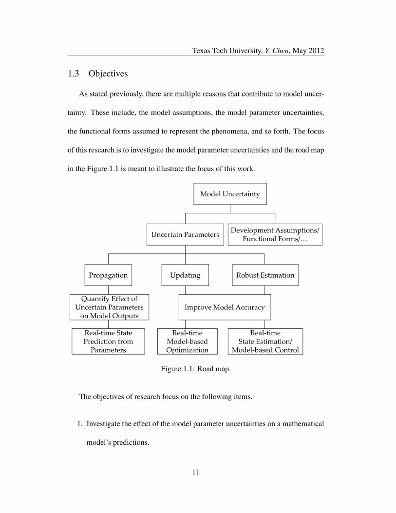
1.3 Objectives
As stated previously, there are multiple reasons that contribute to model uncer-
tainty. These include, the model assumptions, the model parameter uncertainties,
the functional forms assumed to represent the phenomena, and so forth. The focus
of this research is to investigate the model parameter uncertainties and the road map
in the Figure 1.1 is meant to illustrate the focus of this work.
Model Uncertainty
De elo e t A u tio /Uncertain Parameters Development Assumptions/ Functional Forms/…
Propagation Updating Robust EstimationPropagation Updating Robust Estimation
Quantify Effect of Q yUncertain Parameters on Model Outputs
Improve Model Accuracy
Real‐time State Prediction from Parameters
Real‐time Model‐based Optimization
Real‐time State Estimation/
Model based ControlParameters Optimization Model‐based Control
Figure 1.1: Road map.
The objectives of research focus on the following items.
1. Investigate the effect of the model parameter uncertainties on a mathematical
model’s predictions.
11

Texas Tech University, Y. Chen, May 2012
By propagating uncertain parameters through a model, the effect of the model
parameter uncertainties on a mathematical model’s predictions can be quan-
tified. By capturing the relationships between the uncertain parameters and
the real-time state prediction, more accurate state estimation can be real-
ized. In this work, Monte Carlo sampling (MCS), Latin hypercube sampling
(LHS) and Latin hypercube sampling with Hammersley sequencing (LHHS)
are used to establish propagation efficiency. Partial least squares regression
is applied to capture the relationships between the uncertain parameters and
the model outputs. Once the relationships are determined, the PLS model
can be used to predict the process states from known values of the parame-
ters. Usually, the process states are of a higher dimension than the number of
uncertain parameters. To make the PLS feasible and efficient, an application
of the Karhunen-Loeve expansion is employed to reduce the dimension but
retain the dominant temporal and spatial characteristics of the process.
2. Update the uncertain parameters efficiently.
When the uncertain parameters are not readily measurable, an initial guess
of their values is unavoidable. However, for accuracy of the application, up-
dating the initial guess of the parameter uncertainties is justified. One of the
objective of this work is to update the uncertain parameters and thus improve
the estimate of the system states. For very complex and nonlinear models, as
12

Texas Tech University, Y. Chen, May 2012
described above, MCMC and EnKF have been used successfully. They will
be embedded in a model-based optimization framework in this work and their
performance will be compared.
3. Estimate robust values of uncertain parameters.
Robust statistics seeks to provide estimating methods that emulate popular
statistical methods, but which are not unduly affected by outliers or other
small departures from model assumptions. Three types of robust estimates
will be studied for robust estimation. They are, the maximum likelihood type
estimates (MLE), the linear combinations of order statistics (L-Estimate), and
the rank estimates derived from suitable rank tests (R-Estimate). This work
will demonstrate that models parameterized by robust estimates of the uncer-
tain parameters can provide more accurate state estimates.
1.4 Organization
The rest of the dissertation is organized as follows. Chapter 2 presents Monte
Carlo Sampling (MCS), Latin hypercube sampling (LHS) and Latin hypercube
sampling with Hammersley sequence (LHHS) techniques for uncertainty propa-
gation. The production of benzene from hydro-dealkylation (HDA) of toluene is
employed in this chapter to compare the propagation efficiency of these sampling
techniques. To study real-time state prediction from uncertain parameters, partial
13

Texas Tech University, Y. Chen, May 2012
least squares (PLS) regression and Karhunen-Loeve (KL) expansion are introduced
in Chapter 3. The performance of the real-time state prediction from uncertain pa-
rameters also is demonstrated using the HDA process. Chapter 4 introduces and
compares two updating techniques, Markov chain Monte Carlo (MCMC) and en-
semble Kalman filter (EnKF). In Chapter 5, the updating techniques are embed-
ded in a real-time model-based optimization framework. A five-spot pattern oil
reservoir system is introduced to demonstrate and compare the MCMC and EnKF
updating methods. Chapter 6 presents an overview of the theory of robust statis-
tics. Based on robust statistics, a new theorem about a maximum likelihood model
is introduced and proven. In Chapter 7, the robustness feature of the maximum
likelihood model is demonstrated in a model predictive control (MPC) framework.
Lastly, Chapter 8 summarizes the contributions of the research and suggests future
work.
14

Texas Tech University, Y. Chen, May 2012
Nomenclature
AM adaptive Metropolis
ARMAX autoregressive moving average exogenous
CFD computational fluid dynamics
DMC dynamic matrix control
EnKF ensemble Kalman filter
GMC generalized model-based control
HDA hydro-dealkylation
IMC internal model control
L-estimate linear combinations of order statistics
KL Karhunen-Loeve
LHS Latin hypercube sampling
LHHS Latin hypercube Hammersley sequence sampling
MCMC Markov chain Monte Carlo
MCS Monte Carlo sampling
MLE maximum likelihood type estimates
MPC model predictive control
PCA principal component analysis
PLS partial least squares
POD proper orthogonal decomposition
QDMC quadratic dynamic matrix control
QMC quasi Monte Carlo
R-estimate estimates derived from rank tests
ROM reduced-order model
15
Texas Tech University, Y. Chen, May 2012
Chapter 2
Preliminaries on Uncertainty Propagation
This chapter presents an overview of sampling methods of Monte Carlo, Latin
hypercube sampling, and Latin hypercube sampling with Hammersley sequencing
for uncertainty propagation. The production of benzene from hydro-dealkylation
(HDA) of toluene is then introduced to compare the propagation efficiency of these
sampling methods.
With known distributions, for example from historical data, of the multiple un-
certain variables, efficient and effective sampling are reasonable expectations to
propagate the large number of sequences through the complex model to determine
the state estimates and their distributions.
The conventional sampling method of Monte Carlo sampling (MCS) is known
to have low efficiency for uncertainty propagation. As a stratified sampling tech-
nique, Latin hypercube sampling (LHS) technique, is more accurate and efficient
than MCS when there is a single uncertain variable. But in the case of multiple
uncertain variables it has been demonstrated that the efficiency of LHS decreases
noticeably. Another sequencing method, Hammersley sequencing, when combined
with Latin hypercube sampling (LHHS) has been shown to be very efficient when
there are multiple uncertain variables [14].
16

Texas Tech University, Y. Chen, May 2012
2.1 Sampling Techniques
2.1.1 Monte Carlo Sampling
There is no consensus on how Monte Carlo should be defined. For example,
Ripley [55] reserved Monte Carlo for most probabilistic modeling as stochastic
simulation. Sawilowsky [56] distinguished between Monte Carlo method and a
Monte Carlo simulation. A Monte Carlo method can be used to solve a mathe-
matical or statistical problem but a Monte Carlo simulation repeated sampling to
investigate the properties of a phenomenon. Anderson [57] defined Monte Carlo
as the art of approximating an expectation by the sample mean of a function of
simulated random variables.
Monte Carlo sampling (MCS) method is one of the best known methods for
sampling a probability distribution that is based on the use of a pseudo-random
number generator [16]. This simple random sampling involves repeatedly forming
random values of a variable from a prescribed probability distribution. Because the
characteristic of Monte Carlo samples is random, to sample the distribution of an
uncertain variable means a very large number of sample points to cover the distri-
bution range and approximate the real expectation. The large number of sample
points is the primary reason that causes the computational burden for uncertainty
propagation.
To sample an uncertain variable X with MCS, the cumulative distribution func-
17

Texas Tech University, Y. Chen, May 2012
tion (CDF) F of X should be known. The values of the CDF are Pri = F(xi), where
F is the cumulative density function. The procedure is as follows.
• Randomly sample N values of Pri with uniform distribution ranging from 0
to 1, U (0, 1) (i = 1, · · · ,N), where N is the number of sample points and Pri
is a value of the cumulative probability.
• Transform the probability values Pri into the value xi using the inverse of the
distribution function F−1 : xi = F−1(Pri).
2.1.2 Latin Hypercube Sampling
Latin hypercube sampling (LHS) is a stratified-random 1 procedure which pro-
vides an efficient way of sampling a variable from its distribution. The LHS in-
volves sampling N values from the prescribed distribution of the variable X. The
cumulative distribution for this variable is divided into N equally probable intervals.
From each interval a value is selected randomly. Unlike simple random sampling
of MCS, this method ensures a full coverage of a variable by maximally stratifying
its marginal distribution 2 The procedure is as follows.
• Divide the cumulative distribution of the variable into N equal probable in-
1Stratified means that the range of a variable’s distribution has been separated in several intervals.Stratified-random means from each of the divided interval a sample is collected randomly.
2A distribution function may be for more than one variables for example f(x,y) which is the jointdistribution of x and y, the marginal distribution refers to the distribution of one of them f (x) =∫
y( f (x, y)dy. Stratifying the marginal distribution means separating the marginal distribution rangeaveragely according to the number of samples that we want.
18

Texas Tech University, Y. Chen, May 2012
tervals.
• Randomly select a value from each interval. The sampled cumulative proba-
bility can be written as [58]
Pri = (1/N)ru + (i − 1)/N
where ru is a uniformly distributed random number, ru ∼ U (0, 1).
• Transform the probability value Pri into the value Xi using the inverse of the
distribution function F−1 : Xi = F−1(Pri).
Assume 5 sample points of a normal distribution variable X are sampled with
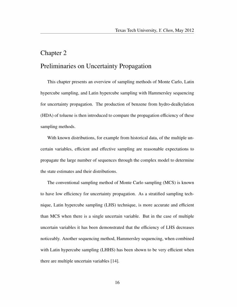
MCS and LHS. X ∼ N (0, 1). Figure 2.1 shows how MCS and LHS select values
for Pri.
It is easy to demonstrate that LHS can use less sample points than MCS to
cover the full range of a variable distribution. Better one-dimensional uniformity
is indicated by the closeness of the sample points to the 45 line with a uniform
interval between the adjacent sample points [14]. As shown in Figure 2.2, for 20
sample points selected by MCS and LHS, the latter shows better uniformity than
the former.
The attractive uniformity property of the LHS method can provide efficient
propagation of LHS sample points for a one dimension uncertain parameter. How-
19
Texas Tech University, Y. Chen, May 2012
-2 -1 0 1 20
0.2
0.4
0.6
0.8
1
X
Cum
ulat
ive
Pro
babi
lity
-2 -1 0 1 20
0.2
0.4
0.6
0.8
1
X
Cum
ulat
ive
Pro
babi
lity
Figure 2.1: Selection of Pri. Top: MCS random selection. Bottom: LHS selectionfrom equal probable intervals.
20

Texas Tech University, Y. Chen, May 2012
0 0.2 0.4 0.6 0.8 10
0.2
0.4
0.6
0.8
1
X
Cum
ulat
ive
Pro
babi
lity
0 0.2 0.4 0.6 0.8 10
0.2
0.4
0.6
0.8
1
X
Cum
ulat
ive
Pro
babi
lity
Figure 2.2: One-dimensional uniformity analysis with 20 sample points. Top:MCS. Bottom: LHS.
21

Texas Tech University, Y. Chen, May 2012
ever, it has been shown that for multiple uncertain distributions, LHS cannot retain
this advantage. Assume there are two variables X and Y and both have uniform dis-
tributions between 0 and 1, that is, X ∼ U (0, 1), Y ∼ U (0, 1). Figure 2.3 compares
the uniformity property of MCS and LHS in two dimensions. One hundred sample
points are generated on a unit square by each sampling method. The figure shows
that the sample points of both MCS and LHS are not ordered.
2.1.3 Latin Hypercube Hammersley Sampling
To combine sample points of multiple dimension variables, the conventional
approach is to pair them randomly. It is in this step that Hammersley sequencing
has better multi-dimensional uniformity [15, 59].
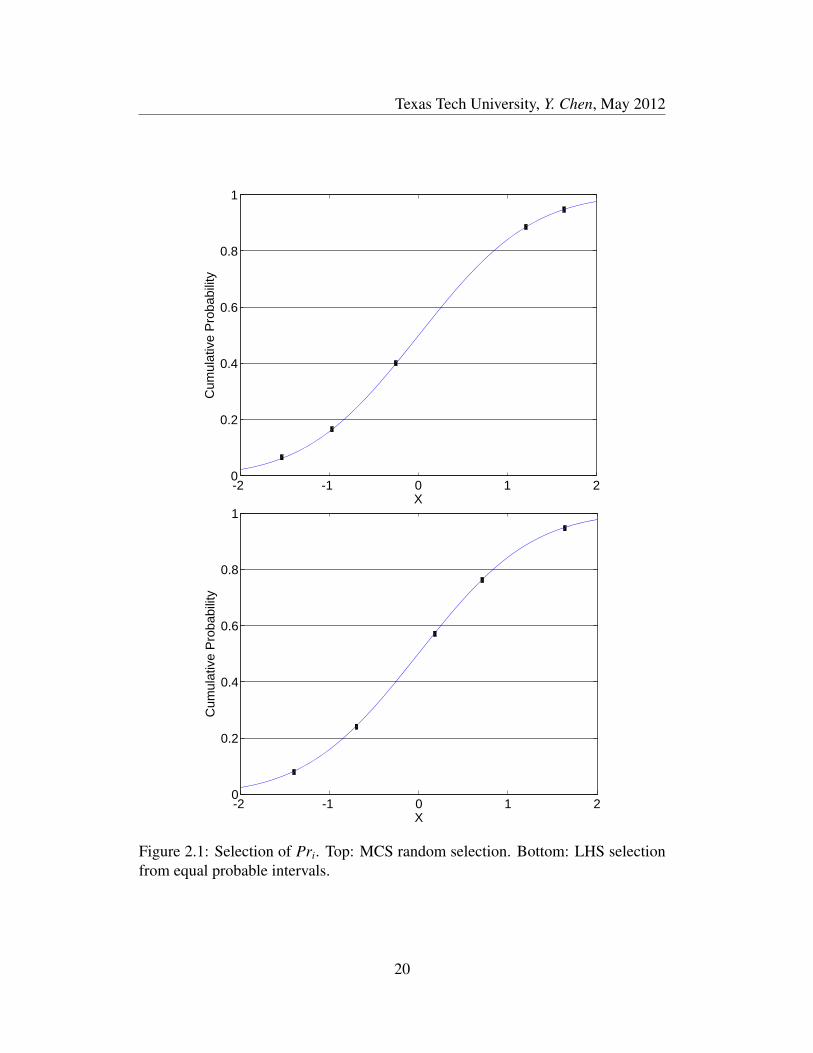
2.1.3.1 Hammersley sequence points
The definition of Hammersley points and an explanation of the procedure to
generate the Hammersley points are as follows [15, 16].
Let any nonnegative integer K be expanded using a prime base p,
K = k0 + k1 p + k2 p2 + · · · + km pm (2.1)
where each k j, j = 1, · · · ,m, is an integer in [0, p-1], m = [logKp ] (square brackets
denote the integral part).
22

Texas Tech University, Y. Chen, May 2012
0 0.2 0.4 0.6 0.8 10
0.2
0.4
0.6
0.8
1
x
y
0 0.2 0.4 0.6 0.8 10
0.2
0.4
0.6
0.8
1
x
y
Figure 2.3: One hundred sample points on a unit square with X,Y ∈ (0, 1). Top:MCS. Bottom: LHS.
23
Texas Tech University, Y. Chen, May 2012
Inverse of prime numbers can be used to define a function φp(K):
φp(K) =k0
p+
k1
p2 + · · · +km
pm+1
The sequence of Hammersley points of dimension d is given by,
(KN, φp1(k), φp2(k), · · · , φpd−1(k)
), K = 1, · · · ,N
where N is the number of samples and p1, · · · , pd−1 are the first d-1 prime numbers.
2.1.3.2 Combination of Latin hypercube sampling and
Hammersley sequencing
In order to retain the uniformity of LHS for multiple dimensions variables,
Hammersley sequence is applied to arrange the LHS sample points of each vari-
able [14, 17]. This sampling method is Latin hypercube Hammersley sampling
(LHHS). Based on the use of rank correlations [60], the LHS sample points for
multi-dimensional variables can be arranged according to the order of the multiple
dimensional Hammersley sequence points.
Suppose X is an N × d matrix that consists of N sets of d uncorrelated pa-
rameters (sampled with LHS). Then the correlation matrix is an identity matrix I .
24

Texas Tech University, Y. Chen, May 2012
Let
C = Γ × Γ′
be the desired correlation matrix ofX where Γ is a lower triangular matrix obtained
by Cholesky factorization. The transformed matrixXΓ′ then has the desired corre-
lation matrix C. This is the theoretical basis for transforming a desired correlation
to an uncorrelated matrix.
Because X is to be rearranged according to the Hammersley sequence points,
these points should be a matrix with the same dimension as X , N × d. Denote
the Hammersley sequence points by the matrixH . With the desired correlation C,
transformH to the rank matrixH∗ whose correlation matrix is C.
To avoid the problem that the correlation matrix of H is not I but R, a matrix
S should be found out that
SRS′ = C
With Cholesky factorization,
R = QQ′
Therefore, the solution of S can be obtained,
S = ΓQ−1
25
Texas Tech University, Y. Chen, May 2012
and correspondingly the transformation factor for the rank matrix is S and the rank
matrix becomes
H∗ =HS′
As a result the correlation matrix of H∗ is exactly equal to the desired matrix
C. The sample matrixX therefore can be paired according to the rank matrixH∗.
In the case of LHS, H is not used and the sample matrix X is rearranged ac-
cording to the correlation matrixC. In the case of the LHHS method ,the matrix of
Hammersley sequence points H is used to rearrange X . According to the defini-
tion of the Hammersley sequence points, these points are distributed uniformly in a
multiple-dimensional space. However, for LHS, uniform distribution is for each di-
mension. When these dimensions are combined the property of uniformity is weak.
In the case of MCS, since it is based on a random score, the uniformity property is
not applicable even when considering one dimension.
Revisiting the two variables case, X ∼ U (0, 1) and Y ∼ U (0, 1). Figure 2.4
shows 100 sample points on a unit square sampled with the LHHS method. When
compared with Figure 2.3, it is observed that these 100 sample points cover the unit
square evenly. In other words, there are no sparse spaces or clot points visible when
compared to Figure 2.3.
If we compare the uniformity property of the MCS, LHS, and LHHS methods in
two-dimensions, Figure 2.3 and 2.4 show that the LHHS generated points have bet-
26

Texas Tech University, Y. Chen, May 2012
ter uniformity properties. The main reason is that the Hammersley sequence places
the sampled points on a multi-dimensional hypercube in an ordered fashion. In con-
trast, the LHS method while designed for uniformity along a single dimension in the
case of multiple dimensions, it randomly pair the sampled points for placement on a
multi-dimensional hypercube. In the case of MCS, even for a single dimension, the
uniformity property is not applicable. Therefore, the likelihood that the MCS and
LHS methods can provide good uniformity property on multi-dimensional cubes is
extremely small.
In the case that there are correlations between the multiple parameters, the
LHHS method still shows the best uniformity property when compared to the MCS
and LHS methods. Once again revisiting the two variables X and Y case, X ∼
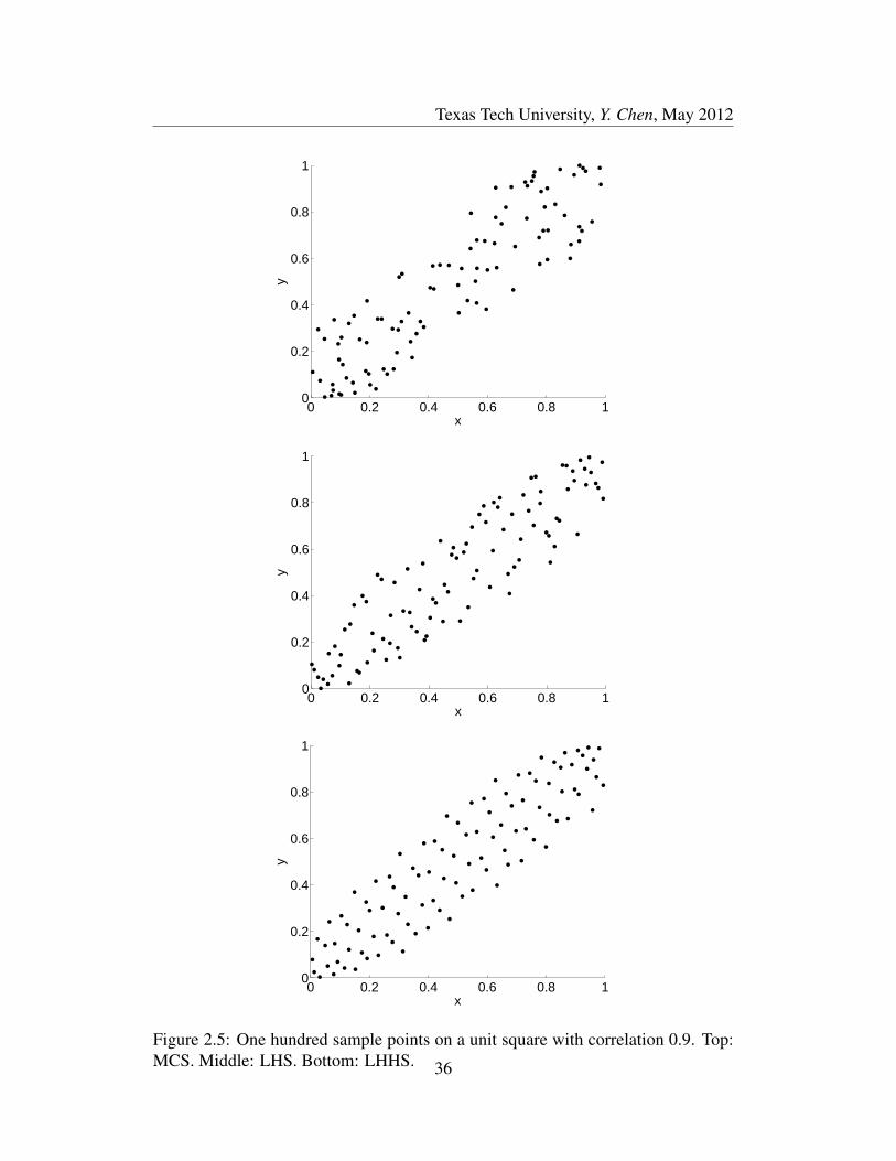
U (0, 1), Y ∼ U (0, 1). Assume the correlation matrix between X and Y is
C =
1 0.9
0.9 1
A rank correlation H∗ = HC can be used to design each dimension. Figure
2.5 shows the uniformity property when there is a desired correlation matrix C for
a two-dimensional uniform distribution of 100 sample points with the imposed 0.9
correlation. As before, it is not difficult to conclude that the LHHS generated points
have better uniformity property when compared to the other methods. The reason
27

Texas Tech University, Y. Chen, May 2012
for this is that the Hammersley sequence preserves the uniformity property.
2.2 Example: HDA Process
The chemical process of benzene production from hydro-dealkylation (HDA)
of toluene [61] is introduced to demonstrate the sampling methods.
2.2.1 HDA Process
The hydro-dealkylation of toluene occurs in a nonlinear plug-flow reactor (PFR)
system (see Figure 2.6) which has been studied extensively by Zheng and Hoo
[7, 2].
Two reactions are known to occur, namely
C7H8 + H2 → C6H6 + CH4
2C6H6 C12H10 + H2
The first reaction is irreversible and the second is an equilibrium reaction. A
28

Texas Tech University, Y. Chen, May 2012
first-principles model can be developed to describe the major reaction phenomena.
∂ε1
∂τ= −υ
(∂ε1
∂τ1+ε1
θ
∂θ
∂τ1
)− ε1ε
0.52 θ
1.5eγ(θ−1/θ)1
∂ε2
∂τ= −υ
(∂ε2
∂τ1+ε2
θ
∂θ
∂τ1
)− ε1ε
0.52 θ
1.5eγ(θ−1/θ)1 + κ2(ε3θ)2eγ
(θ−1/θ)2 − κ3ε2ε5θ
2eγ(θ−1/θ)3
∂ε3
∂τ= −υ
(∂ε3
∂τ1+ε3
θ
∂θ
∂τ1
)+ ε1ε
0.52 θ
1.5eγ(θ−1/θ)1 − 2κ2(ε3θ)2eγ
(θ−1/θ)2 + 2κ3ε2ε5θ
2eγ(θ−1/θ)3 + FBm
∂ε4
∂τ= −υ
(∂ε4
∂τ1+ε4
θ
∂θ
∂τ1
)+ ε1ε
0.52 θ
1.5eγ(θ−1/θ)1
∂ε5
∂τ= −υ
(∂ε5
∂τ1+ε5
θ
∂θ
∂τ1
)+ κ2(ε3θ)2eγ
(θ−1/θ)2 − κ3ε2ε5θ
2eγ(θ−1/θ)3
∂θ
∂τ=
1ζ
[Hr1∂ε1
∂τ− Hr2
∂ε5
∂τ+ Q(θF − θ) − v
(ζ∂θ
∂τ1− Hr1
∂ε1
∂τ1+ Hr2
∂ε5
∂τ1
)]− FBmζB
(2.2)
where ζ = (Cp/CP0)(P0/Pr), υ(z) = (Fin + Fin j)/(P/RT ), Fin is the feed to the reac-
tor, εi is the concentration of the ith component and θ is the dimensionless reactor
temperature. The initial feed concentrations (mole fraction) of toluene, hydrogen,
and methane are ε1,0 = 0.0807, ε2,0 = 0.4035, ε4,0 = 0.5158. Table 2.1 provides
the definition and values of the parameters and variables, and subscript 0 is the
reference condition.
The boundary conditions are:
z = 0, εi = εi(t = 0), i = 1, · · · , 5, θ = θ(t = 0)
z = 1,∂εi
∂z= 0, i = 1, · · · , 5,
∂θ
∂z= 0
The pure benzene stream is injected at the start of the reactor. The finite difference
solution of this system serves as the true solution.
29

Texas Tech University, Y. Chen, May 2012
Table 2.1: Dimensionless parameters for the HDA process [2].
Parameter Nominal values Definition
P = Pr/P0 1.0 Reactor pressure
FBm = Fin j/Fin 0.008 Dimensionless benzene injection
θF = TF/T0 1.0 Jacket temperature
κ1 = k1(T0)/k1(T0) 1.0 Dimensionless reaction 1 rate constant
κ2 = k2(T0)P20/k1(T0)P1.5
0 0.995 Ratio of reaction 1 to reverse reaction 2
κ3 = k3(T0)P20/k1(T0)P1.5
0 5.34 Ratio of reaction 1 to reverse reaction 3
Hr1 = HR1/Cp0T0 -1.51 Heat of reaction 1
Hr2 = HR2/Cp0T0 -0.473 Heat of reaction 2
Q 0.0 Heat transfer coefficient
γ1 = Ea/RT0 29.26 Reaction 1 activation energy
γ2 = Ea/RT0 29.68 Reaction 2 activation energy
γ3 = Ea/RT0 33.49 Reaction 3 activation energy
τ ∈ <+ > 0 Dimensionless time
z ∈ Ω [0,1] Dimensionless space
2.2.2 Propagation with Different Sampling Methods
Each parameter in the HDA process is not exact, but not all of the parameters
have a pronounced effect on the system solution. Using a parametric sensitivity
analysis, the outputs are found to be most sensitive to the rate constant of reaction 1
(κ1), the fresh benzene injection rate (FBm), and the heat of reaction 1 (Hr1). These
parameters are uncorrelated.
Assume that a Gaussian distribution can represent each of these three param-
30
Texas Tech University, Y. Chen, May 2012
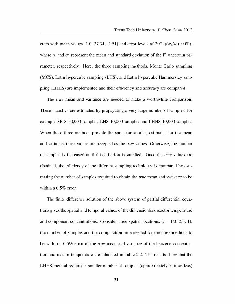
eters with mean values 1.0, 37.34, -1.51 and error levels of 20% ((σi/ui)100%),
where ui and σi represent the mean and standard deviation of the ith uncertain pa-
rameter, respectively. Here, the three sampling methods, Monte Carlo sampling
(MCS), Latin hypercube sampling (LHS), and Latin hypercube Hammersley sam-
pling (LHHS) are implemented and their efficiency and accuracy are compared.
The true mean and variance are needed to make a worthwhile comparison.
These statistics are estimated by propagating a very large number of samples, for
example MCS 50,000 samples, LHS 10,000 samples and LHHS 10,000 samples.
When these three methods provide the same (or similar) estimates for the mean
and variance, these values are accepted as the true values. Otherwise, the number
of samples is increased until this criterion is satisfied. Once the true values are
obtained, the efficiency of the different sampling techniques is compared by esti-
mating the number of samples required to obtain the true mean and variance to be
within a 0.5% error.
The finite difference solution of the above system of partial differential equa-
tions gives the spatial and temporal values of the dimensionless reactor temperature
and component concentrations. Consider three spatial locations, z = 1/3, 2/3, 1,
the number of samples and the computation time needed for the three methods to
be within a 0.5% error of the true mean and variance of the benzene concentra-
tion and reactor temperature are tabulated in Table 2.2. The results show that the
LHHS method requires a smaller number of samples (approximately 7 times less)
31

Texas Tech University, Y. Chen, May 2012
when compared to the LHS and is superior to the MCS (approximately 60 to 70
times less samples). For the same accuracy, LHHS is most efficient of these three
methods.
Figure 2.7 shows the standard deviations of the dimensionless benzene concen-
tration and reactor temperature that result with the implementation of the different
sampling methods at the exit of the reactor. The upper and lower solid lines give
the error limits of ± 0.5% of the true standard deviation. True standard deviation
of the benzene concentration is 1.033 × 10⁻³ and that of the reactor temperature is
1.782 × 10⁻³. It can be found that the LHHS method uses least number of sample
points to be within the error range and to have the fastest convergence rate.
The effect of the propagation of the parameter uncertainties through the model
is shown in Figure 2.8, which shows the distributions of the dimensionless ben-
zene concentration and reactor temperature at the reactor exit. The probability of
the model output uncertainties caused by uncertain parameters can be obtained by
propagation.
2.3 Summary
This chapter introduced three sampling techniques, Monte Carlo sampling (MCS),
Latin hypercube sampling (LHS), and Latin hypercube sampling with Hammersley
sequencing (LHHS). Their uniform property are explained to compare their sam-
pling efficiency. These three sampling techniques are applied in hydro-dealkylation
32

Texas Tech University, Y. Chen, May 2012
Tabl
e2.
2:C
ompu
tatio
ntim
ean
dnu
mbe
rofs
ampl
esat
thre
esp
atia
lloc
atio
nsth
atac
hiev
es0.
5%er
roro
fthe
true
mea
nan
dva
rian
ceof
the
benz
ene
conc
entr
atio
nan
dre
acto
rtem
pera
ture
.
z=1/
3z=
2/3
z=1
Met
hod
MC
SL
HS
LH
HS
MC
SL
HS
LH
HS
MC
SL
HS
LH
HS
Tim
eB
enco
nc15
2.1
15.6
2.1
114.
113
1.9
86.9
131.
9(m
in)
Tem
p18
7.3
15.6
2.1
182
15.6
1.9
14.1
15.6
1.9
Sam
ple
Ben
conc
5600
600
9042
0050
080
3200
500
80Te
mp
6900
600
9067
0060
080
4200
600
80
33

Texas Tech University, Y. Chen, May 2012
(HDA) of toluene process which illustrates the advantage of LHHS over MCS and
LHS. The product of LHHS technique is the generation of the outputs and their
uncertainty distributions that are functions of the uncertainty in the parameters.
34

Texas Tech University, Y. Chen, May 2012
0 0.2 0.4 0.6 0.8 10
0.2
0.4
0.6
0.8
1
x
y
Figure 2.4: One hundred sample points (sampled with LHHS) on a unit square withx, y ∈ (0, 1).
35
Texas Tech University, Y. Chen, May 2012
0 0.2 0.4 0.6 0.8 10
0.2
0.4
0.6
0.8
1
x
y
0 0.2 0.4 0.6 0.8 10
0.2
0.4
0.6
0.8
1
x
y
0 0.2 0.4 0.6 0.8 10
0.2
0.4
0.6
0.8
1
x
y
Figure 2.5: One hundred sample points on a unit square with correlation 0.9. Top:MCS. Middle: LHS. Bottom: LHHS. 36

Texas Tech University, Y. Chen, May 2012
Feed
FB BenzeneQuench
z = 0 z = 1
51 L=iiε
Outputcomponents
C7H8
H2 CH4
C7H8 H2
C6H6 CH4
C12H10
Figure 2.6: Plug Flow Reactor.
37

Texas Tech University, Y. Chen, May 2012
0 1000 2000 3000 4000 50001.015
1.025
1.035
1.045
1.055
1.06 x 10⁻³
Number of sample points
Sta
ndar
d de
viat
ion
of b
enze
ne c
once
ntra
tion
0 1000 2000 3000 4000 50001.72
1.74
1.76
1.78
1.8
1.82
1.84 x 10⁻³
Number of sample points
Sta
ndar
d de
viat
ion
of d
imen
sion
less
tem
pera
ture
Figure 2.7: Standard deviation of benzene concentration (left) and reactor temper-ature (right) as a function of sample size. +: MCS. : LHS. ?: LHHS.
38

Texas Tech University, Y. Chen, May 2012
0.04 0.05 0.06 0.07 0.08 0.090
0.02
0.04
0.06
0.08
0.1
0.12
0.14
Dimensionless benzene concentration
Pro
babi
lity
1.02 1.04 1.06 1.08 1.1 1.120
0.02
0.04
0.06
0.08
0.1
0.12
0.14
0.16
Dimensionless temperature
Pro
babi
lity
Figure 2.8: Distribution of dimensionless benzene concentration and temperature.
39

Texas Tech University, Y. Chen, May 2012
Nomenclature
CDF cumulative distribution function
HDA hydro-dealkylation
LHHS Latin hypercube Hammersley sampling
LHS Latin hypercube sampling
MCS Monte Carlo sampling
PDE partial differential equation
C correlation matrix H matrix of Hammersley pointsH∗ rank matrx K integer
N number of sample points Pr probability value
X random variables Y random variablesd dimension of uncertain variables ru uniformly distributed random valueφp function of Hammersley points N normal distributionU uniform distribution
40

Texas Tech University, Y. Chen, May 2012
Chapter 3
Real-time State Prediction
Chapter 3 investigates real-time state prediction as a function of the set of un-
certain parameters using partial least squares regression (PLS) and the Karhunen-
Loeve (KL) expansion. These concepts are demonstrated using the HDA process
that was introduced in Chapter 2.
As stated previously, a first-principles model that describes the behavior of a
process is a system of nonlinear partial differential equations (PDEs) in which the
variables are function of space and time. Solving such systems is time consuming
and the solutions are an infinite series that cannot be used readily for real-time
applications such as real-time state prediction. However, if there are data that carry
the relationships between the process state variables and the uncertain parameters,
then a technique such as partial least squares (PLS) regression may be suitable to
capture these relationships in a less computationally-burdensome regression-type
model to enable real-time prediction.
3.1 PLS Regression
In order to consider the effects of uncertain parameters on the state variables, it
is necessary to determine the relationships between the uncertain parameters and the
41

Texas Tech University, Y. Chen, May 2012
data set of solutions generated from the first-principles model. Partial least squares
(PLS) regression is an often used method to determine the relationships between
the prediction variables and response variables.
The following is excerpted from [62]. Let XN×I be a matrix of I predictors
collected on N observations that describe J response variables, Y N×J. Decompose
both X and Y as a product of a set of orthogonal factors (T ) and a set of loadings
(P ),
X = TP ′ +E
Y = TBC′ + F
(3.1)
The columns of T are the latent vectors, P is the coefficient matrix of X , the
diagonal elements ofB are the regression weights,C represents the weights of the
response variables, and E and F are the matrices of residual errors.
To specify the latent vectors in T , two sets of weights w and c are needed to
create a linear combination of the columns of X and Y such that their covariance
is maximized. The goal is to obtain a pair of vectors t = Xw and u = Y c with
constraints such that w′w = 1, t′t = 1. It then follows that p =X ′t.
Procedurally, let Q = X and R = Y . Then column center and normalize R
andQ.
Step 1: Initialize the vector u with random values
Step 2: Estimate weights forX , w ∝ Q′u
42

Texas Tech University, Y. Chen, May 2012
Step 3: EstimateX factor scores, t1 = Qw1
Step 4: Estimate weights for Y , c1 ∝ R′t1
Step 5: Estimate Y scores, u1 = Rc1
Step 6: Return to step 2 if t1 has not converged. Otherwise continue.
Step 7: Calculate b = t′1u1
Step 8: Compute the loadings forX: p1 = Q′T .
Step 9: Subtract the effect of t1 from both Q and R: Q = Q − t1p′1 and R =
F − bt1c′1. b is a diagonal element ofB.
Step 10: Repeat from step 1 until the matrixQ becomes null.
The symbol ∝ represents a normalization of the result. The above relations
show thatw1 is the first right singular vector ofX ′Y and c1 is the first left singular
vector of X ′Y . Similarly, t1 and u1 are the first eigenvectors of XX ′Y Y ′ and
Y Y ′XX ′, respectively [62].
The prediction of the dependent variables is based on a multivariate regression
given by,
Y = TBC′ =XBPLS (3.2)
whereBPLS = (P ′)−1BC′.
43
Texas Tech University, Y. Chen, May 2012
3.2 KL Expansion
In some chemical processes such as a reactor, the states, for example, temper-
ature, concentration and so forth are functions of time and space whose data sets
have a larger dimension than the dimension of the uncertain parameters. To make
the PLS model feasible initial pre-processing of the data with a method such as
Karhunen-Loeve (KL) expansion is necessary, since the KL method can reduce the
dimension of the state data sets.
The basic concept behind the KL expansion is to find those modes that repre-
sent the dominant character of the system such that the basis set corresponding to
these modes comprise what is called the empirical eigenfunctions (EEFs) of the
system. The number of EEFs is usually small, which brings about a dimensionality
reduction without a loss in the complexity that is inherent to distributed parameter
systems [63].
Consider Equations (3.3) and (3.4) that represent the state and measured out-
puts, respectively of a simple one-dimensional (1D) PDE that can be used to repre-
sent a variety of nonlinear phenomena. Here, z is the spatial variable defined on a
closed and compact domain Ω, t is time, y(z, t) are the outputs, x(z, t) are the state
44
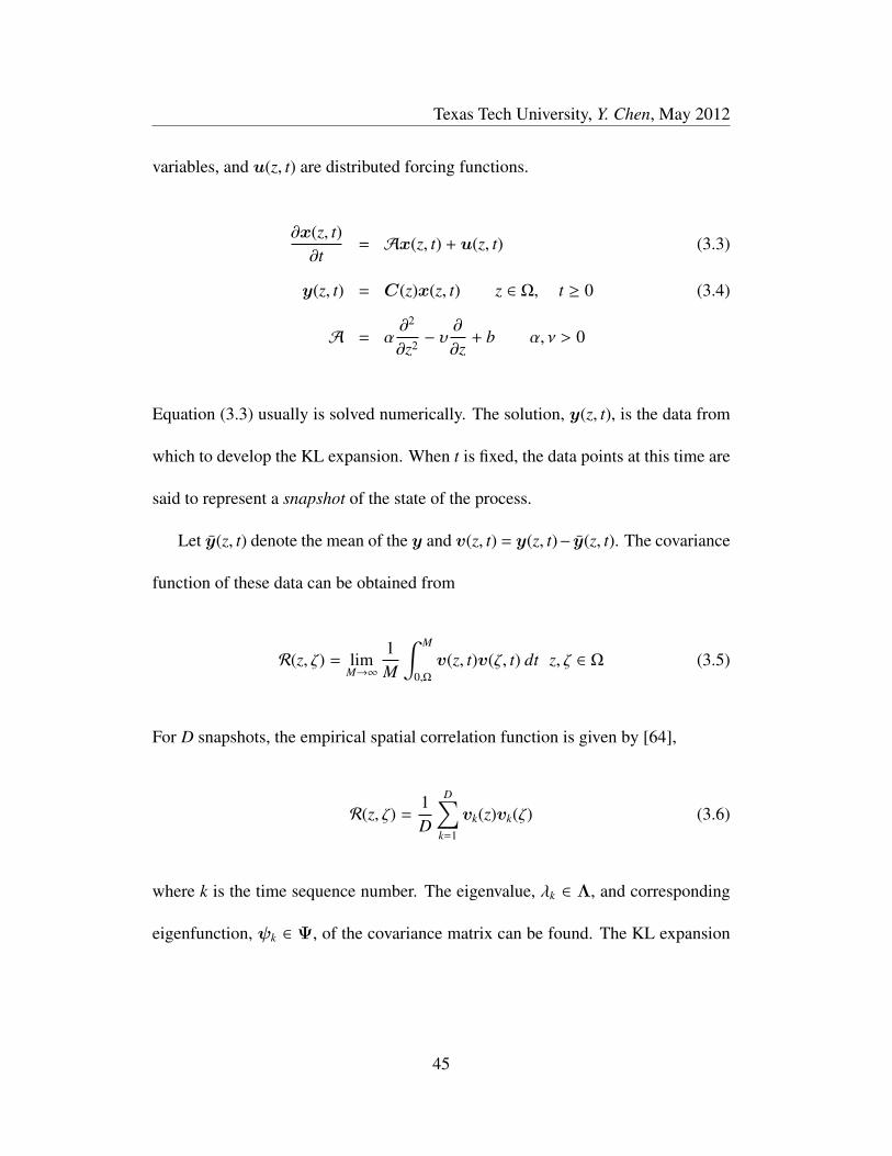
Texas Tech University, Y. Chen, May 2012
variables, and u(z, t) are distributed forcing functions.
∂x(z, t)∂t
= Ax(z, t) + u(z, t) (3.3)
y(z, t) = C(z)x(z, t) z ∈ Ω, t ≥ 0 (3.4)
A = α∂2
∂z2 − υ∂
∂z+ b α, ν > 0
Equation (3.3) usually is solved numerically. The solution, y(z, t), is the data from
which to develop the KL expansion. When t is fixed, the data points at this time are
said to represent a snapshot of the state of the process.
Let y(z, t) denote the mean of the y and v(z, t) = y(z, t)− y(z, t). The covariance
function of these data can be obtained from
R(z, ζ) = limM→∞
1M
∫ M
0,Ωv(z, t)v(ζ, t) dt z, ζ ∈ Ω (3.5)
For D snapshots, the empirical spatial correlation function is given by [64],
R(z, ζ) =1D
D∑k=1
vk(z)vk(ζ) (3.6)
where k is the time sequence number. The eigenvalue, λk ∈ Λ, and corresponding
eigenfunction, ψk ∈ Ψ, of the covariance matrix can be found. The KL expansion
45

Texas Tech University, Y. Chen, May 2012
of the system defined in Equation (3.3) is given by,
y(z, t) = y(z, t) +∞∑
k=1
√λk ψk(z)ςk(t) (3.7)
where ςk are the projections of y onto ψk. It has been shown that a small number
of EEFs can capture more than 95% of the system’s energy [65] in many instances
indicting a high degree of correlation among the data or a small number of degrees
of freedom in the data [60].
3.3 State Prediction with ROM
In this work, PLS regression is applied to determine the relationships between
the uncertain parameters and the state data sets obtained from the first-principles
model. The dimension of the state data sets is reduced using a KL expansion to
build a reduced-order model (ROM). Since Latin hypercube Hammersley sequence
(LHHS) has good multiple-dimensional uniformity property, it is used to sample
the set of uncertain parameter distributions. The sample sequences are propagated
through the first-principles model. By averaging the resulting state data sets, the
dominant empirical eigenfunctions (EEFs) of the averaged data matrix can be de-
termined. The EEFs serve as the basis for propagation of the state data. Usually a
small number of EEFs can capture the dominant characteristics of the data. With
a small number of dominant EEFs, the corresponding coefficients also is small.
46
Texas Tech University, Y. Chen, May 2012
These coefficients are the response variables for PLS regression. With the sampled
sets of uncertain parameters as predictors, the relationships between the uncertain
parameters and the coefficients of the corresponding propagated data matrices can
be determined with PLS regression to identify a predictive model. Then, given any
set of uncertain parameters, the ROM coefficients can be calculated from the iden-
tified PLS model. It then follows that the ROM’s outputs which are the states can
be predicted directly by projection of the coefficients onto the EEFs. Thus, with
the combination of PLS regression and KL expansion execution of the complex,
nonlinear first-principles model is avoided. To summarize, the procedural steps are
as follows.
• Step 1: Sample multiple uncertain parameters with LHHS technique.
• Step 2: Propagate samples of uncertain parameters (sampled in Step 1) through
first-principles model. Solve models with samples of uncertain parameters to
obtain the corresponding model outputs.
• Step 3: Average the model outputs and use KL expansion to reduce the di-
mension of averaged matrix to determine its dominant EEFs.
• Step 4: Calculate the corresponding coefficients of all the model outputs ob-
tained in step 2 based on the EEFs calculated in step 3.
• Step 5: Determine the relationships between the samples of uncertain param-
47

Texas Tech University, Y. Chen, May 2012
eters (sampled in Step 1) and the corresponding coefficients of model outputs
(calculated in Step 4) to build a PLS model.
• Step 6: Predict the process states from known values of the parameters with
the PLS model obtained in step 5.
3.3.1 State Prediction of HDA Process
The HDA process that was introduced in Chapter 2 will be used to demonstrate
state prediction using a ROM generated from the combination of PLS regression
and KL expansion. The uncertain parameters are the rate constant of reaction 1
(κ1), the fresh benzene injection rate (FBm) and the heat of reaction 1 (Hr1). The
parameter distributions assumed in Chapter 2 remain unchanged. The data sets are
the numerical solutions to the system of PDEs that describe the HDA process. This
set includes five component concentrations and the reactor temperature.
A means of validating the generated ROM is as follows. For the same set of in-
put parameters compare the outputs of the ROM to the outputs of the first-principles
model. Furthermore, in order to test if the outputs of the ROM generated from the
uncertain data can track the outputs of the first-principles model better than the out-
puts of a ROM generated from data without uncertainty, a ±5% bias in the mean
values and +20% error in the standard deviations of the uncertain parameters are
introduced.
48

Texas Tech University, Y. Chen, May 2012
Figures 3.1 to 3.3 compare the benzene concentration and the reactor tempera-
ture, determined using the ROMs with and without uncertainty propagation against
the results of the physical model in the presence of the bias and error in the stan-
dard deviation of the uncertain parameters, respectively. From these figures, it is
observed that the outputs of the ROM generated from data with uncertainty can
track the outputs of the physical model satisfactorily.
The maximum relative errors between the first-principles model and the ROM
are listed in Table 3.1. It is shown that with the same bias of the parameters mean
values and errors in their standard deviations, the ROM generated with uncertain
data has less error.
Table 3.1: Maximum relative errors in the outputs between the physical model andthe ROM with and without uncertainty.
µi: +5% bias µi: -5% bias σi: +20% std
ROM Benz Temp Benz Temp Benz Temp
With uncertainty +3.47% +0.22% -9.95% -0.49% +2% +0.51%
Without uncertainty -12.21% -0.74% -23.56% +0.88% +9.22% +0.81%
3.4 Summary
Partial least squares (PLS) regression is applied to determine the relationships
between the uncertain parameters and the model outputs. To reduce the high di-
mension of the data sets, the Karhunen-Loeve (KL) expansion is employed. Two
49

Texas Tech University, Y. Chen, May 2012
0 0.2 0.4 0.6 0.8 10
0.01
0.02
0.03
0.04
0.05
0.06
0.07
0.08
z (m) - Dimensionless length of reactor
Ben
zene
con
cent
ratio
n
0 0.2 0.4 0.6 0.8 10.98
1
1.02
1.04
1.06
1.08
1.1
z (m) - Dimensionless length of reactor
Dim
ensi
onle
ss te
mpe
ratu
re
Figure 3.1: Output of the ROM and physical model in the presence of a +5% biasin the mean value of the uncertain parameters. Left: Benzene concentration. Right:Reactor temperature. 4: Physical model. : ROM generated with uncertain data. ∗:ROM without uncertainty.
50

Texas Tech University, Y. Chen, May 2012
0 0.2 0.4 0.6 0.8 10
0.01
0.02
0.03
0.04
0.05
0.06
0.07
z (m) - Dimensionless length of reactor
Ben
zene
con
cent
ratio
n
0 0.2 0.4 0.6 0.8 10.97
1
1.03
1.06
1.09
z (m) - Dimensionless length of reactor
Dim
ensi
onle
ss te
mpe
ratu
re
Figure 3.2: Output of the ROM and physical model in the presence of a -5% biasin the mean value of the uncertain parameters. Left: Benzene concentration. Right:Reactor temperature. 4: Physical model. : ROM generated with uncertain data. ∗:ROM without uncertainty.
51

Texas Tech University, Y. Chen, May 2012
0 0.2 0.4 0.6 0.8 10
0.01
0.02
0.03
0.04
0.05
0.06
0.07
0.08
z (m) - Dimensionless length of reactor
Ben
zene
con
cent
ratio
n
0 0.2 0.4 0.6 0.8 10.98
1
1.02
1.04
1.06
1.08
1.1
z (m) - Dimensionless length of reactor
Dim
ensi
onle
ss te
mpe
ratu
re
Figure 3.3: Output of the ROM and physical model in the presence of a +20% errorin the standard deviation of the uncertain parameters. Left: Benzene concentration.Right: Reactor temperature. 4: Physical model. : ROM generated with uncertaindata. ∗: ROM without uncertainty.
52

Texas Tech University, Y. Chen, May 2012
reduced-order models (ROMs) are generated, one with and the other without knowl-
edge of the uncertainties. The results of these two ROMs are then compared to the
outputs from the first-principles model. In the presence of parameter uncertainties,
the ROM that is generated by knowledge of the uncertainties has a smaller error
when compared against the outputs from the first-principles model. The hydro-
dealkylation (HDA) of toluene process was used to demonstrate these concepts.
53

Texas Tech University, Y. Chen, May 2012
Nomenclature
EEF empirical eigenfunction
HDA hydro-dealkylation
LHHS Latin hypercube Hammersley sampling
KL Karhunen-Loeve
PDE partial differential equation
PLS partial least squares
ROM reduced-order model
X predictors Y response variablesx state variables y outputsz space variable λ eigenvalueψ eigenfunction ς coefficientN normal distribution U uniform distribution
54

Texas Tech University, Y. Chen, May 2012
Chapter 4
Preliminaries on Uncertain Parameter Updating
As stated before, some parameters are not measurable in some complex condi-
tions, such as geography, meteorology and oceanography. In many instances there
is almost no information about the value of these parameters. To obtain accurate
estimates of the process behavior from a descriptive model, the parameters of the
model are updated at some frequency using information from the measured vari-
ables.
Based on Bayes’ theorem, a number of approaches called particle filters or se-
quential Monte Carlo techniques are used to estimate values of the uncertain pa-
rameters. This chapter introduces and compares two recursive filters, Markov chain
Monte Carlo (MCMC) filter and the ensemble Kalman filter (EnKF) for uncertain
parameters updating. The contents of this chapter are excerpted from [38, 66].
One of the reasons that Bayesian methods are so attractive to use in uncertain
parameter updating is that they can incorporate prior knowledge through the as-
sumed known information, which is then combined with actual observed data to
update and eventually converge to a final and accurate estimation of the parameter
values.
MCMC methods are a class of algorithms for sampling from a proposed param-
55

Texas Tech University, Y. Chen, May 2012
eter probability distribution based on constructing a Markov chain for each parame-
ter that has the desired distribution as its stationary distribution. The final variables’
stationary distributions give the estimates of the uncertain parameters. The EnKF
is a Monte Carlo implementation of the Bayesian update problem, basically using
an ensemble of model parameter values to evaluate the necessary statistics.
4.1 Markov Chain Monte Carlo
The Markov chain Monte Carlo (MCMC) methods generate parameter values
from a constructed Markov chain, which converges to a stationary distribution. Al-
though there are many different MCMC algorithms, the general steps are as follows.
1. At iteration i = 0; arbitrarily choose an initial parameter value Θ = Θ0
2. (a) Generate a candidate value Θ∗ for Θ from a proposed distribution de-
pending on the current value Θi.
(b) Compute an acceptance probability α that depends on Θ∗, Θi, the pro-
posed distribution, the model, and the observed data.
(c) Accept Θi+1 = Θ∗ with probability α; otherwise, Θi+1 = Θi.
3. Increment i and repeat step 2 until a stationary distribution of the parameter
is achieved.
Marshall et al discussed the study of MCMC methods for conceptual rainfall-
runoff modeling [30]. Two MCMC algorithms were compared: a conventional
56

Texas Tech University, Y. Chen, May 2012
Metropolis-Hastings algorithm and an adaptive Metropolis (AM) algorithm. The
study showed that the AM algorithm was superior in many respects and can offer a
relatively simple basis for assessing parameter uncertainty.
4.1.1 Adaptive Metropolis Algorithm
The AM algorithm can generate all the uncertain model parameter values in a
single iteration [30].
1. At iteration i = 0 choose an arbitrary variable vector Θ = Θ0. Candidate
values of this vector, Θ∗, are generated from a proposed probability density
function according to the current values Θi of Θ.
2. Compute the acceptance probability, α that is a function of Θi, Θ∗, the model
and observed data. If the candidate value Θ∗ is accepted with acceptance
probability
α = min
1,P(y|Θ∗)P(Θ∗)P(y|Θi)P(Θi)
(4.1)
then Θi+1 = Θ∗; otherwise Θi+1 = Θi. Here P(Θ) is the prior distribution of
Θ and P(y|Θ) is the likelihood function of the observed data y with model
M,
P(y|Θ) = (2πσ2ε)−N/2exp
−∑N
j=1[y j − M(Θ)]2
2σ2ε
(4.2)
N is the number of data points, M(Θ) is the in silico model outputs, and Θ
57

Texas Tech University, Y. Chen, May 2012
is the vector of uncertain model parameters. The error term is ε = y − M(Θ)
and σ2ε is its variance.
The proposed distribution of the parameters is a multi-normal distribution that has
mean values at the current point, Θi, and a covariance matrix [30]. The covariance
matrix, Ci, has a fixed value C0 for the first i0 iterations and is updated according to
the following rule,
Ci =
C0 i ≤ i0
sdCov(Θ0, · · · ,Θi−1) i > i0
(4.3)
where sd is a scaling parameter that depends on the dimensionality, d, of Θ. A large
value of i0 will result in a slower adaptation [23]. Thus, the size of i0 reflects our
trust in the initial covariance C0. The initial covariance C0 is an arbitrary strictly
positive-definite matrix chosen according to the best prior knowledge.
The empirical covariance of Θ1, · · · ,Θk ∈ Rd, is given by,
Cov(Θ1, · · · ,Θk) =1
k − 1
k∑i=1
Θi(Θi)′ − kΘk(Θk)′ (4.4)
where
Θk =1k
k∑i=1
Θi
58

Texas Tech University, Y. Chen, May 2012
and the elements Θi ∈ Rd are column vectors. For i ≥ i0 + 1, the covariance Ci
satisfies the recursion formula:
Covi+1 =i − 1
iCovi +
sd
i
[iΘi−1(Θi−1)′ − (i − 1)Θi(Θi)′ +Θi(Θi)′
](4.5)
When the dimension d (the number of uncertain parameters) is large, the prior
distribution will converge at a slower rate to the stationary distribution. The work
of [67] has shown that a value of sd = (2.38)2/d will yield asymptotic optimality of
accepting rate for d ≤ 6.
In the AM algorithm, the covariance of the first i0 iterations is unchanged, but
thereafter the covariance is updated according to Equation (4.3). The proposed val-
ues of the uncertain parameters are generated from Equation (4.6) using the ith pa-
rameter values as the mean. The initial number of iterations in the MCMC method
can be selected to be large, however, the tradeoff is a high computing burden.
As an example, suppose that Θ is a vector with two elements Θ = [Θ1 Θ2]′.
The following function f is the probability density function of uncertain parameters.
f (Θ1,Θ2) =1
2πσ1σ2
√1 − ρ2
×
exp
−(Θ1 − µ1)2
σ21
−2ρ(Θ1 − µ1)(Θ2 − µ2)
σ1σ2+
(Θ2 − µ2)2
σ22
2(1 − ρ2)
(4.6)
59
Texas Tech University, Y. Chen, May 2012
where µi, σi, i = 1, 2 are the mean and standard deviation of Θi and ρ is the corre-
lation coefficient of Θi j. The covariance matrix for this bivariate normal is given
by
Cov(Θ1,Θ2) =
σ11 σ12
σ21 σ22
=σ2
1 ρσ1σ2
ρσ2σ1 σ22
(4.7)
4.2 Ensemble Kalman Filter
The EnKF is a recursive filter. When compared to the standard Kalman filter, the
notable difference is that the covariance matrix is replaced by the sample covariance
computed from the ensemble data. An advantage of the EnKF method is that it can
do updating in very nonlinear systems. The EnKF is a Monte Carlo implementation
of the Bayesian update problem, basically using an ensemble of model parameters
to evaluate the necessary statistics. This method consists of a forecast step and a
assimilation step in which the state variables and uncertain parameters are corrected
based on the current observations. The assimilation step has been described as the
step that attempts to update the uncertainty based on the measurements.
The EnKF is developed by sequentially running a forecast step followed by an
assimilation step. The inputs to the forecast (y fk+1) step are the results obtained
from the assimilation (yak ) step that are updates of the uncertain parameters after
the inclusion of the current set of observed data. The forecast step is the simulator
advanced in time.
60

Texas Tech University, Y. Chen, May 2012
4.2.1 Forward Step
The EnKF is initialized by generating an initial ensemble described by,
ya0,i = y
a0 + e0,i i = 1, . . . ,Ne (4.8)
where Ne is the total number of members in the ensemble; ya0 is the initial mean of
the ensemble members; and e0,i is the error.
The state vector yk,i consists of two parts: all the variables Θ that are uncertain
and the in silico data denoted by d,
yk,i =
s
−
d
k,i
= [Θ1,Θ2, · · · ,ΘD, d1, d2, · · · ]Tk,i (4.9)
where D is the number of uncertain parameters. The index i means the ith ensemble
member; and d1, d2, · · · are the individual datum in the observation vector d.
The forecast step includes execution of the process model and providing an
expression for the uncertainty in the model output. In the forecast step, the model
is executed from time k − 1 to k when the next observation data are available,
y fk,i = f
(ya
k−1,i
)i = 1, . . . ,Ne, k = 1, . . . ,N (4.10)
61

Texas Tech University, Y. Chen, May 2012
Each member of the ensemble is used in one execution of the process model.
The relationship between the observed and predicted state vectors is given by,
dobs,k,i =Hkytrue + εk,i i = 1, . . . ,Ne, k = 1, . . . ,N (4.11)
where εi is assumed to be Gaussian distributed with zero mean and covariance
Qd,k; Hk ∈ RNd,k×Ny,k is an operator that relates the actual state to the theoretical
observation [36]; Nd,k is the number of observations; and Ny,k is the number of
variables in the state vector at time k. Since the in silico data d are a part of y (see
Equation (4.9)), the elements in Hk can be assigned values of 0 or 1, thus Hk can
be arranged as
Hk =
[0 | I
](4.12)
where 0 is an Nd,k × (Ny,k − Nd,k) matrix of zeros, and I is a Nd,k × Nd,k identity
matrix.
4.2.2 Assimilation Step
The assimilation step incorporates y fk . The state vector y(k) can be updated
based on a difference between the observed data and the in silico data. The weight-
ing matrix at time step k is the Kalman gain,Kk,
yak,i = y
fk,i +Kk
(dobs,k,i −Hky
fk,i
)k = 1, . . . ,N i = 1, . . . ,Ne (4.13)
62

Texas Tech University, Y. Chen, May 2012
Let Y fk ∈ RNy,k×Ne denote the ensemble of forecast state vectors at time k, and
Y fk ∈ RNy,k×1 as the mean of the state variables calculated from the current ensemble
members,
yk,i =(yk,1,yk,2, · · · ,yk,Ne
)(4.14)
The covariance matrix for the state variables at any step k is estimated from the
forecast ensemble,
P fk =
1Ne − 1
(Y f
k − Yf
k
) (Y f
k − Yf
k
)Tk = 1, . . . ,N (4.15)
where the covariance between mth and the nth variables (m, n = 1, . . . ,Ny and i =
1, . . . ,Ne), pm,n ∈ Pf
k , is obtained from
pm,n =1
Ne − 1
Ne∑i=1
(y f
m,i − yfm
) (y f
n,i − yfn
)(4.16)
Here, ym and yn are the means of the mth and nth variables, respectively calculated
from the ensemble members of the state vector. The Kalman gain matrix is a func-
tion of the covariances,
Kk = Pf
k HTk
(HkP
fk H
Tk +Qd,k
)−1(4.17)
63

Texas Tech University, Y. Chen, May 2012
4.3 Example
An example, a nonlinear logistic map equation, is presented to demonstrate
these concepts. MCMC and EnKF are used to update the state according to the
measurements. The logistic equation is Equation (4.18) [68]
xk+1 = axk(1 − xk)
yk+1 = xk+1
(4.18)
where a is a parameter, 1 ≤ a ≤ 4; 0 < x < 1 is the state variable and y is the output
that can be measured. When a = 3.5, the outputs of the logistic map equation are
four distinct values 0.875, 0.8269, 0.5009, 0.3828 as shown in Figure 4.1. Figures
4.2 and 4.3 show the estimated state based on the MCMC and EnKF methods. The
initial guess values of x for both MCMC and EnKF are the same. For MCMC, 1000
points are used to form a Markov chain and for EnKF 100 elements are used as an
ensemble. In 100 steps, both MCMC and EnKF show satisfactory state updating
and estimation for the nonlinear logistic map.
4.4 Summary
In this chapter, two updating methods for estimating the uncertain parameters in
a nonlinear model are presented. A simple example is employed to demonstrate the
updating performance of MCMC and EnKF. In the next chapter, the Markov chain
64

Texas Tech University, Y. Chen, May 2012
0 10 20 30 40 50
0.4
0.5
0.6
0.7
0.8
0.9
1
Step k
Out
puts
from
logi
stic
equ
atio
n
Figure 4.1: Outputs of the logistic map.
0 20 40 60 80 100
0.4
0.5
0.6
0.7
0.8
0.9
1
Step k
MC
MC
sta
te e
stim
atio
n
Figure 4.2: State estimation with MCMC.
65
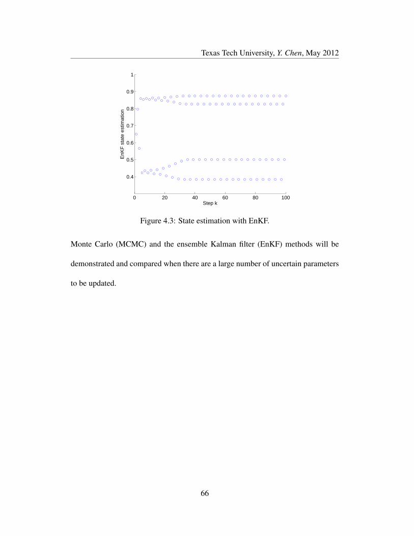
Texas Tech University, Y. Chen, May 2012
0 20 40 60 80 100
0.4
0.5
0.6
0.7
0.8
0.9
1
Step k
EnK
F st
ate
estim
atio
n
Figure 4.3: State estimation with EnKF.
Monte Carlo (MCMC) and the ensemble Kalman filter (EnKF) methods will be
demonstrated and compared when there are a large number of uncertain parameters
to be updated.
66

Texas Tech University, Y. Chen, May 2012
Nomenclature
AM adaptive Metropolis
EnKF ensemble Kalman filter
MCMC Markov chain Monte Carlo
C covariance of Markov chain H matrix operatorI identity matrix K Kalman gain matrixN number of observations in MCMC Nd number of observationsNe number of ensemble members Ng number of grid blocksNy number of state vector elements P state variables covarianceP likelihood function Qd measurement covarianceT transpose Y ensemble of state vectorsd model output data dobs measured data in EnKFe error term k time steps model parameters sd scaling parametery measured data in MCMC ya assimilated estimates of the statesy f forecast of the states ε measurement errorΘ uncertain parameters vector σ standard deviation
67

Texas Tech University, Y. Chen, May 2012
Chapter 5
Real-time Model-based Optimization with Parameter Up-
dating
In this chapter, parameter updating is embedded in a real-time model-based
optimization framework. A five-spot pattern oil reservoir system is introduced to
demonstrate and compare the Markov chain Monte Carlo (MCMC) and ensemble
Kalman filter (EnKF) updating methods. The contents of this chapter are excerpted
from [38, 66].
5.1 Uncertain Parameter Updating in a Model-Based Optimization
Framework
Figure 5.1 shows a framework that combines model-based optimization with
model parameter updating.
At each step, the uncertain parameters in the first-principles model are updated
using the measurements from the nonlinear system and a new reduced-order model
(ROM) is identified from the updated first-principles model.
5.2 Updating in a Reservoir Management Framework
Figure 5.2 is a simple schematic of a reservoir.
68

Texas Tech University, Y. Chen, May 2012
Nonlinear System
d
u
ym
First Principles Model(Θ)
Optimizer
Low-orderModel
MCMCy(Θ)
e
++
+-
y*
Nonlinear System
d
u
ym
Optimizer
Reduced OrderModel
Update
y(Θ)
e
++
+-
y*
First Principles Model(Θ)
Figure 5.1: Model-based optimization framework with parameter uncertainty up-dating. y∗: set-points; u: outputs from the optimizer; d: disturbances; ym: mea-surements; y(Θ): model outputs; Θ: model uncertain parameters; e: errors be-tween measurements and model outputs.
Injection well 2
Injection well 4
Injection well 1
Injection well 3
Production well
I II
III IV
Figure 5.2: Schematic of a two-dimensional reservoir and wells. ↓: water injectionwell; ↑: oil production well.
5.2.1 Reservoir
Many different patterns can be selected to represent the reservoir. Here, one of
the most well-known patterns, a five-spot pattern is chosen [69]. The water injection
wells are located at the four corners of the reservoir and the oil well is located in
the middle of the reservoir. The reservoir covers an area of 630×630 ft2 and has a
69

Texas Tech University, Y. Chen, May 2012
thickness of 30 ft. This region is modeled by a 9×9×1 horizontal two-dimensional
grid blocks. The fluid system consists of two phases, oil and water, with 0.1 connate
water saturation and 0.3 residual oil saturation.
A first-principles model for this two-phase reservoir with immiscible porous
media flow and isotropic permeability can be described by,
∇
(krokµoBo
∇po
)=∂
∂t
(φS o
Bo
)+
qo
V
∇
(krwkµwBw
∇pw
)=∂
∂t
(φS w
Bw
)+
qw
V
S o + S w = 1
po − pw = Pc(S w)
(5.1)
where ∇ is the gradient operator; the subscripts o and w represent oil and water,
respectively; and S o and S w are oil and water saturation; Pc is the capillary pressure
which is the force to squeeze oil droplets through porous media. It works against
the interface tension between oil and water phases. The definition of the variables
and parameters can be found in Table 5.1.
The first-principles model is a system of nonlinear partial differential equations
that is not trivial to solve numerically. However, there are commercial reservoir
simulation software that are available and may provide a solution that represents
the temporal and spatial behavior of the system. The solution provided by the com-
mercial software also can be used as in silico data to supplement historical data so
70

Texas Tech University, Y. Chen, May 2012
Table 5.1: Definition of Model Variables and Parameters.
Variable Definition Unit
k absolute permeability miliDarcykr relative permeability %µ viscosity centipoiseB formation volume factor RB/STB (real barrels/standard barrels)p pressure psiPc capillary pressure psiφ porosity %qo oil production rate STBD (standard barrels/day)qw water injection rate STBDS fluid phase saturation %V reservoir volume ft3
t time day
that an input-output model of the reservoir can be identified. Such models are usu-
ally preferred in real-time model-based optimization since they are computationally
less burdensome. In this work, the reservoir software ECLIPSE (Schlumberger Co,
Houston, TX), version 2009.1, is used to provide in silico data to identify a ROM
for the purposes of optimal management of an oil producing reservoir.
In order to solve a reservoir model, the values of parameters in the model should
be known. As described before, the values of the parameters may contain uncer-
tainty. The especially serious problem is when there is no consensus on values for
some of the reservoir parameters because of the changing geographic conditions.
Porosity and permeability are two such parameters that suffer from this problem.
Porosity is a fraction of the void volume over the total volume of a material. How
much oil or water that is contained in a reservoir totally depends on the porosity.
71
Texas Tech University, Y. Chen, May 2012
Permeability is a measure of the ability of a porous material to allow fluids to pass
through it. Thus, how much oil can be pushed out of the reservoir mainly depends
on the material’s permeability. We can conclude that porosity and permeability
are two of the key parameters whose values are essential to providing an accurate
simulation of oil production from a reservoir.
Because of the changing geographic structure, a single effective value of either
porosity or permeability ought not to be assumed. In this work, the reservoir is
divided into several grids and each grid is assumed to have a single effective value of
porosity and permeability. As the number of grids increase so too does the accuracy
of the simulation but at the expense of a huge computational burden.
The values of porosity and permeability are measured by experimenting on the
rock cores which can be obtained by drilling a reservoir. The common way to mea-
sure the porosity is to use imbibition method. The weight of vacuumed rock sample
is measured at beginning. The vacuumed rock sample is immersed in a liquid envi-
ronment and then weighted again. The weight difference between the rock sample
after soaking up the liquid and the vacuumed rock sample is then calculated. With
the density of the liquid, the volume of the void spaces in the rock sample can be
computed. The porosity is the ratio between the volume of the void spaces and
the volume of the rock sample. Permeability is typically determined by applying
Darcy’s law to experiment on a rock sample. Darcy’s law describes the flow of a
fluid through a porous medium. Darcy’s law (see Equation (5.2)) is a proportional
72

Texas Tech University, Y. Chen, May 2012
relationship between the discharge rate of a fluid through a porous medium, the fluid
viscosity and the pressure difference over a given distance of the porous medium.
Q =−kAµ
∆PL
(5.2)
To measure the permeability k of a rock sample, a liquid is forced to flow through
the sample. In Equation (5.2) Q is the discharge rate of the liquid; µ is the liquid
viscosity; A is the cross-sectional area of the rock sample; ∆P is the pressure drop,
which is the difference between the exit liquid pressure from the rock sample and
its input liquid pressure; and L is the length of the rock sample. The permeability k
of the rock sample can be calculated with the measurements of Q, A, ∆P, L and the
liquid viscosity according to Equation (5.2) .
The rock samples are obtained by drilling wells in a reservoir. It is impossible
and expensive to drill everywhere in a reservoir to obtain all the samples that repre-
sents the entire geographic structure. The porosity and permeability at the position
where there is a well can be measured. But their values everywhere else are not
known. We can conclude that in a reservoir, the values of porosity and permeability
have a large amount of uncertainty. Then, in an in silico model of the reservoir that
is constructed as a grid, in almost every grid the values of porosity and permeabil-
ity are not known with any certainty. It is reasonable that these model parameters
should be updated whenever measurements from the reservoir are known to main-
73

Texas Tech University, Y. Chen, May 2012
tain model accuracy.
Assume that the true porosity and permeability distributions are in the intervals
[0.04, 0.33] and [6, 600] miliDarcy, respectively [70] (see Figures 5.7 and 5.8). The
outputs of the reservoir model are generated by execution of the ECLIPSE model
with the true parameters and the addition of noise to the oil and water production
values, water cut (the ration of the production of water over the total production of
oil and water), and bottom hole pressures (BHPs, BHP is the pressure at the bottom
of the hole of a well). The measurement uncertainties are presented in Table 5.2.
Table 5.2: Measurement uncertainties. [3]
Quantity ±σ
Oil production 5%
Water production 5%
Bottom hole pressures 1 bar
5.2.2 Basic Optimization Problem
Maximizing the potential production capability of an oil or gas reservoir is the
aim of the real-time model-based reservoir management framework. This frame-
work, referred to as a closed-loop management approach, is modified from Figure
5.1 to include parameter updating and illustrated in Figure 5.3.
The ECLIPSE commercial software provides a fundamental model of the reser-
voir that when executed with feasible initial conditions and known reservoir size
74
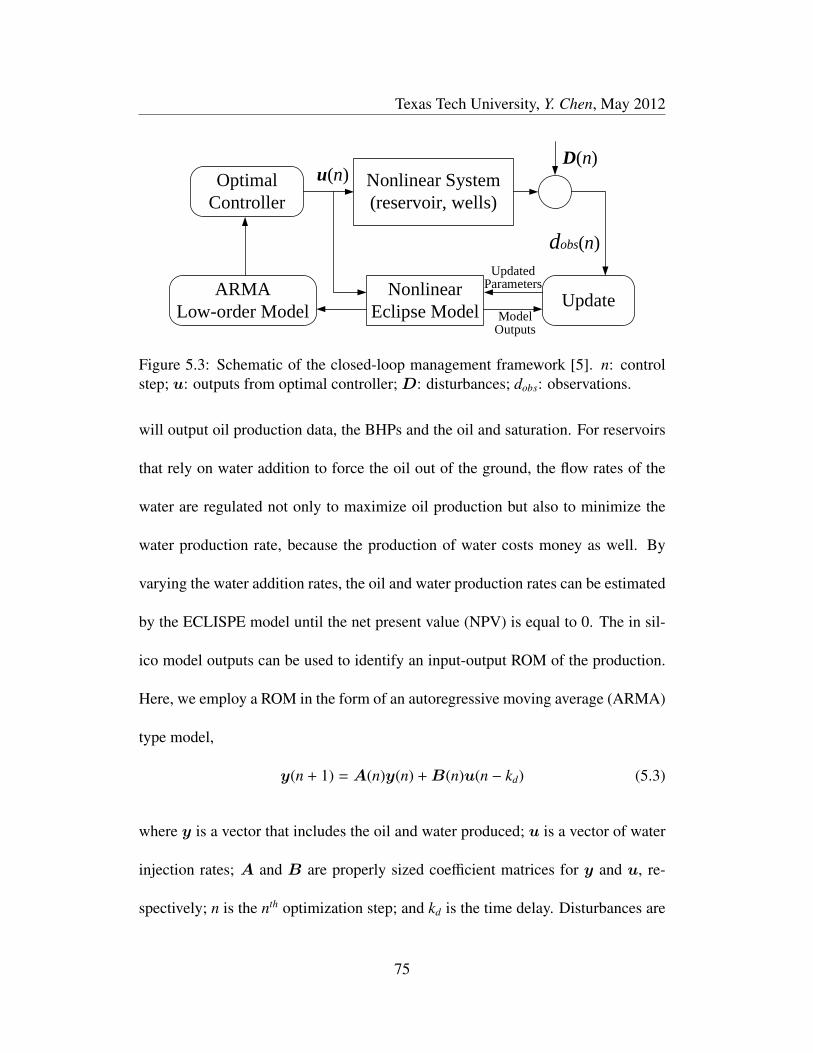
Texas Tech University, Y. Chen, May 2012
Nonlinear System(reservoir, wells)
OptimalController
D(n)u(n)
dobs(n)
EnKFARMALow-order Model
NonlinearEclipse Model yf(n)
ya(n)
Nonlinear System(reservoir, wells)
OptimalController
D(n)u(n)
dobs(n)
UpdateARMALow-order Model
NonlinearEclipse Model Model
Outputs
UpdatedParameters
Figure 5.3: Schematic of the closed-loop management framework [5]. n: controlstep; u: outputs from optimal controller;D: disturbances; dobs: observations.
will output oil production data, the BHPs and the oil and saturation. For reservoirs
that rely on water addition to force the oil out of the ground, the flow rates of the
water are regulated not only to maximize oil production but also to minimize the
water production rate, because the production of water costs money as well. By
varying the water addition rates, the oil and water production rates can be estimated
by the ECLISPE model until the net present value (NPV) is equal to 0. The in sil-
ico model outputs can be used to identify an input-output ROM of the production.
Here, we employ a ROM in the form of an autoregressive moving average (ARMA)
type model,
y(n + 1) = A(n)y(n) +B(n)u(n − kd) (5.3)
where y is a vector that includes the oil and water produced; u is a vector of water
injection rates; A and B are properly sized coefficient matrices for y and u, re-
spectively; n is the nth optimization step; and kd is the time delay. Disturbances are
75
Texas Tech University, Y. Chen, May 2012
not considered in this study.
To generate the ARMA model, at each optimization step, different sets of water
well injection rates (u = u(0), . . . ,u(n)) are used by the ECLIPSE model to
generate estimates of the oil and water production (y = y(0), . . . ,y(n)).
Maximizing the NPV is the objective of the optimization,
L = maxN∑
n=1
Ln (5.4)
where N is the total number of optimization steps. The NPV for each step is defined
as [71]
Ln =∆tn
(1 + a)tn
Nprod∑j=1
(roqn
o, j − rwqnw, j
) (5.5)
where ∆t is the length of the optimization step; Nprod is the number of producers;
and ro and rw are respectively, the benefit and cost coefficients of oil and water
production. The denominator of the first term represents the effect of discounting
where a is the discounting factor and tn is the time expressed at the nth optimization
step. Because the value of the discounting factor is constant over a fixed interval
of time, it does not affect either the water or oil production rates. In this work, it
is assumed that the effect of discounting is neglected; i.e., that a = 0 according to
[71, 72]. Maximizing NPV is equivalent to maximizing cumulative oil production
(qo) and minimizing cumulative water production (qw) by adjusting the injected
76

Texas Tech University, Y. Chen, May 2012
water flow rates to each well. The controller outputs are the optimum injected
water flow rates that maximize NPV.
5.2.3 Markov Chain Monte Carlo Updating
As shown in Figure 5.4, the reservoir is divided into three sections (labeled as
I, II, or III), with each section containing three 3×3 connected grids. As mentioned
before in Chapter 4, scaling parameter sd is dependent on the dimensionality and
valid at 6 dimensions or lower. Thus, within each section, the selected uncertain
parameters, porosity and permeability, are assumed to have the same distributions
for a total of 6 uncertain parameters.
With known porosity and permeability data obtained from the analysis of rock
cores, initial distributions of these property values are estimated and assigned to
the reservoir. By comparing the results with known historical data the most ap-
propriate combinations of three grids (see Figure 5.4, which is divided in a 3×3
grid) are selected. Porosity is usually found to have a normal distribution while
permeability is characterized as having a log-normal distribution [73]. As shown
in Figure 5.5, the assigned prior distributions of porosity are: φI −N (0.22, 0.05),
φII −N (0.17, 0.04), φIII −N (0.13, 0.03); and the assigned prior distributions of
permeability are: kI −Nlog(6.17, 0.25), kII −Nlog(5.02, 0.24), kIII −Nlog(3.58, 0.23).
Updates of the parameter distributions require a comparison between the ob-
served data (oil and water production, water cut and BHPs) and the ECLIPSE model
77

Texas Tech University, Y. Chen, May 2012
III
II
I
Injection well 1 Injection well 3
Injection well 2 Injection well 4
Production well
Figure 5.4: Schematic of a two-dimensional reservoir and wells. ↓: water injectionwell; ↑: oil production well.
0 0.1 0.2 0.3 0.4 0.50
0.1
0.2
0.3
0.4
Porosity I
Pro
babi
lity
dens
ity
0 0.1 0.2 0.3 0.40
0.1
0.2
0.3
0.4
Porosity II0 0.1 0.2 0.3
0
0.1
0.2
0.3
0.4
Porosity III
100 550 1000 14500
0.1
0.2
0.3
0.4
Permeability I
Pro
babi
lity
dens
ity
0 100 200 300 4000
0.1
0.2
0.3
0.4
Permeability II10 26 42 58 74 900
0.1
0.2
0.3
0.4
Permeability III
Figure 5.5: Prior distributions of porosity and permeability.
78

Texas Tech University, Y. Chen, May 2012
predictions. This means that a very large number of different combinations of the
samples of the uncertain parameters are input parameters in the ECLIPSE model. In
other words, the ECLIPSE model needs to be executed thousands of times, which
translates to a huge computational burden [66]. To overcome this obstacle, PLS
regression described in Chapter 3 can be applied to find the relationships between
the uncertain parameters and the ECLIPSE model outputs. Thus, execution of the
ECLIPSE reservoir model is supplanted because the outputs can be calculated di-
rectly from the values of uncertain parameters by the PLS regression model. The
execution time to generate the PLS results is at least 10 times less than one execu-
tion of the ECLIPSE model. Thus, the MCMC combined with PLS can improve
the updating efficiency.
Figure 5.6 shows the updated distributions of ki, φi, i = 1, 2, 3. The updated
distributions of φi are: φI−N (0.25, 0.027), φII−N (0.2, 0.018), φIII−N (0.15, 0.015);
and the updated distributions of ki are: kI−Nlog(6.38, 0.088), kII−Nlog(5.23, 0.082),
kIII −Nlog(3.78, 0.086). It is noted that the updated distributions have smaller stan-
dard deviations than those of the prior distributions. This is not unexpected since
with the MCMC technique, the distributions are guaranteed to attain a stationary
distribution.
79

Texas Tech University, Y. Chen, May 2012
5.2.4 Ensemble Kalman Filter Updating
The reservoir state vector consists of all the reservoir variables that are uncer-
tain. There are two parts to the reservoir state vector yk,i: the model parameters s
(including porosity, permeability, pressure and phase saturation) and the in silico
data d (generated by the simulator including oil and water production, water cut
and BHPs),
yk,i =
s
−
d
k,i
=[φ1, · · · , φNg , ln(k1), · · · , ln(kNg), p1, · · · , pNg , S w1, · · · , S wNg , d1, d2, · · ·
]T
k,i
(5.6)
where i is ith ensemble member; Ng is the number of grids in a reservoir; d1, d2, · · ·
are individual datum in the observation vector d; and T denotes transpose of a vec-
tor.
In this work, the ensemble set is chosen to be of size one hundred [26]. Thus,
the assignment of the initial estimation of the porosity and permeability is much
finer with EnKF than that with MCMC. The generation of the error term for the
permeability parameter is based on a spatially correlated Gaussian model that as-
sumes that the permeability in grid block (i1, j1) is correlated with the permeability
80

Texas Tech University, Y. Chen, May 2012
in grid block (i2, j2) [3],
exp[−
( i1 − i2
`
)2
−
( j1 − j2
`
)2](5.7)
The correlation length ` is a normally distributed stochastic variable. A correla-
tion matrix C is computed from Equation (5.7). The covariance matrices used for
generating noise for the permeability ensemble is computed as σ2C where σ is the
standard deviation in the permeability of each grid block.
Based on known values of porosity and permeability obtained from the well’s
rock cores, the initial ensemble values are generated by linearizing the critical pa-
rameter values along the length and width of the reservoir [35]. The measurements
are assimilated everyday for the first 10 days, then every 10 days for 50 days, and
once every month for 11 months. This schedule is chosen according to the work of
[71, 74] but this should not imply that the schedule itself could not be an optimiza-
tion parameter. Results with control steps of 25, 50, and 70 days also were carried
out but not shown here. It was found that the oil and water production differences
are within 0.4% when compared to a 30-day control step.
For comparison, the mean values of porosity and permeability of the initial en-
semble is used as reference to compare the updated results of parameters. Figures
5.7 and 5.8 show k, φ for the true and initial cases and also the updated cases after
30, 180, 240, and 390 days.
81

Texas Tech University, Y. Chen, May 2012
Figures 5.9 and 5.10 show the uncertainties associated with k, φ after 30, 120,
180, 240, 300, and 390 days. The uncertainty associated with the grid blocks that
are closer to the wells is smaller when compared to those that are farther away. Ad-
ditionally, the overall uncertainty decreases as the number of days increases since
more measurements are assimilated.
In Figures 5.11 and 5.12, the forecasts of the measurements for daily oil and
water production, cumulative oil and water production, water cut and BHPs are
shown based on 30, 120, 180, 240, 300, and 390 days. As expected, as more and
more data are assimilated the quality of the forecasts is improved asymptotically.
The mean values of the ensemble can be used as the updated values of k, φ
at each time step. These updated values are inputs to the in silico model to obtain
more data to identify the input-output model (see Equation (5.3)).
5.2.5 Optimal Oil Production Results
In the reservoir, water is injected in the wells, which affects the reservoir’s pres-
sure to displace oil from the reservoir and out the production well. In this work,
800 STBD (standard barrels/day) of water are specified for the well with a min-
imum BHPs of 4000 psia. Additionally, there are minimum and maximum con-
straints for each injection well, in this case 160 and 240 STBD, to ensure that the
maximum BHPs are within 4350 psia. These pressures are chosen to maintain a
pressure balance between the underground and ground surfaces.
82
Texas Tech University, Y. Chen, May 2012
The optimized solution is compared to a non-optimized case. The oil price, ro,
is set at 110$/bbl according to the crude oil price at the end of April, 2011 and water
production costs, rw, are set at 12$/bbl according to [72]. To guarantee that NPV
> 0, the water cut target, qw/(qo + qw) = 0.9 so that the equality roqo − rwqw = 0 is
satisfied.
In this work, the optimizer has a 30 days basis to make a decision. At each
optimization step, the uncertain parameters are updated and an ARMA model is
identified as the ROM in the model-based optimization framework (cf Equation
(5.3)) until the target water cut value of 0.9 is reached. To maximize the NPV in
Equation (5.4), water production (qw) should be minimized while simultaneously
maximizing oil production (qo).
Figure 5.13 shows the topology of the injected water when the water cut equals
0.9 for the non-optimized and optimized cases (with the EnKF and MCMC meth-
ods updating the uncertain parameters respectively. With the updated values of the
uncertain parameters, the ROM is re-identified and used by the optimizer at the next
step. Clearly, the water has saturated the reservoir.
Comparing the graphs in Figure 5.13, the water sweep as determined by the op-
timal closed-loop controller is an improvement over the non-optimized case. More
oil is produced by adjusting the amount of water added in the optimized case; and
at the same time the water saturation values are higher than in the non-optimized
case.
83

Texas Tech University, Y. Chen, May 2012
The top panel of Figure 5.14 shows the cumulative oil and water production
rates of the non-optimized and optimized cases at each step until the water cut is
0.9. For the optimized case with EnKF, the final cumulative oil production increases
7.1% and the final cumulative water production decreases by 10.5% when compared
to the non-optimized case. For the optimized case with MCMC, the final cumulative
oil production increases 5.3% and the final cumulative water production decreases
by 3.4%.
Since the oil production has increased and water production has decreased, the
cumulative NPVs (with EnKF and MCMC updating) also increases significantly
(bottom panel of Figure 5.14), 9.0% (EnKF) and 8.2% (MCMC) more than the
final NPV of the non-optimized case.
Although the geological properties are different for different reservoirs, it is still
meaningful to analyze the effects of permeability and porosity on the adjustment
of the injection water rate with this five-spot pattern reservoir. The reservoir is
divided into four equal size parts with the five wells as shown in Figure 5.2. The
following analysis is based on the EnKF results since the EnKF provides better
updating performance.
The average permeability and porosity in the four parts of reservoir in each
optimization steps are calculated. Figure 5.15 shows a graph of the changes in the
optimal injected water flow rate in the first well as a function of the updating steps
and the average permeability and porosity values at each step. Figures 5.16 to 5.18
84

Texas Tech University, Y. Chen, May 2012
provide a similar graph for the second, third and fourth wells. The z-axis in the
graph is the proportion of the water flow rate in the corresponding well to all the
water flow rates in four injection wells.
Table 5.3 shows the ranges of porosity, permeability and water injection ratio of
the four parts of the reservoir.
Table 5.3: Porosity, permeability and water injection ratio of four parts of reservoir.
Porosity (%) Permeability (miliDarcy) Water injection ratio (%)
I 0.21–0.28 280–350 0.27–0.3
II 0.12–0.16 190-245 0.2–0.25
III 0.21–0.28 209-248 0.27-0.3
IV 0.06–0.10 22-32 0.2
From the graphs and Table 5.3, it can be concluded that the optimal injected wa-
ter flow rates have a strong relationship to the values of permeability and porosity.
When the permeability and porosity are larger, more water can be added to force
the oil out of the reservoir. This is reasonable behavior since a larger porosity value
indicates there is more oil present in the reservoir and a larger permeability value
indicates easier flowability.
The ranges of the porosity and permeability in the fourth part of the reservoir
are smallest when compared to the others, thus the injected water flow rate hovers
around the injected water flow rate lower constraint. In this case, it also can be con-
cluded that porosity has a larger effect on the calculated values of the optimal water
85

Texas Tech University, Y. Chen, May 2012
flow rates than permeability. The first and third parts of the reservoir have the same
range of porosity but different ranges of permeability. However, the optimal flow
rates of the first and third wells are similar to each other. Although the permeability
range in the second part is similar to that of the third part, the optimal water flow
rates in the second well are different from the third well because of the difference
in their porosity ranges.
5.3 Summary
An optimal management approach combined with model parameter updating
was presented. Two updating filtering methods, Markov chain Monte Carlo (MCMC)
and ensemble Kalman filter (EnKF) are designed and compared. Although the
MCMC combined with partial least squares (PLS) can improve the updating ef-
ficiency, the main disadvantage of MCMC is the limitation on the number of un-
certain parameters to be updated. In contrast, the EnKF can update a large number
of uncertain parameters. To make the closed-loop optimization framework com-
putationally manageable while remaining accurate, a reduced-order computational
model (ARMA, autoregressive moving average) is identified that relates the in-
jected water flow rate to oil production. By optimizing the injection water flow
rate, increased oil production and decreased water production resulted in a increase
(9.0% EnKF, 8.2% MCMC) in the final cumulative net present value. An analysis
of the results revealed that the values of permeability and porosity have important
86

Texas Tech University, Y. Chen, May 2012
effects on the optimal adjustment of the injected water flow rates. Thus, updating
the values of these two uncertain parameters played an important role in optimal
management of the reservoir.
87
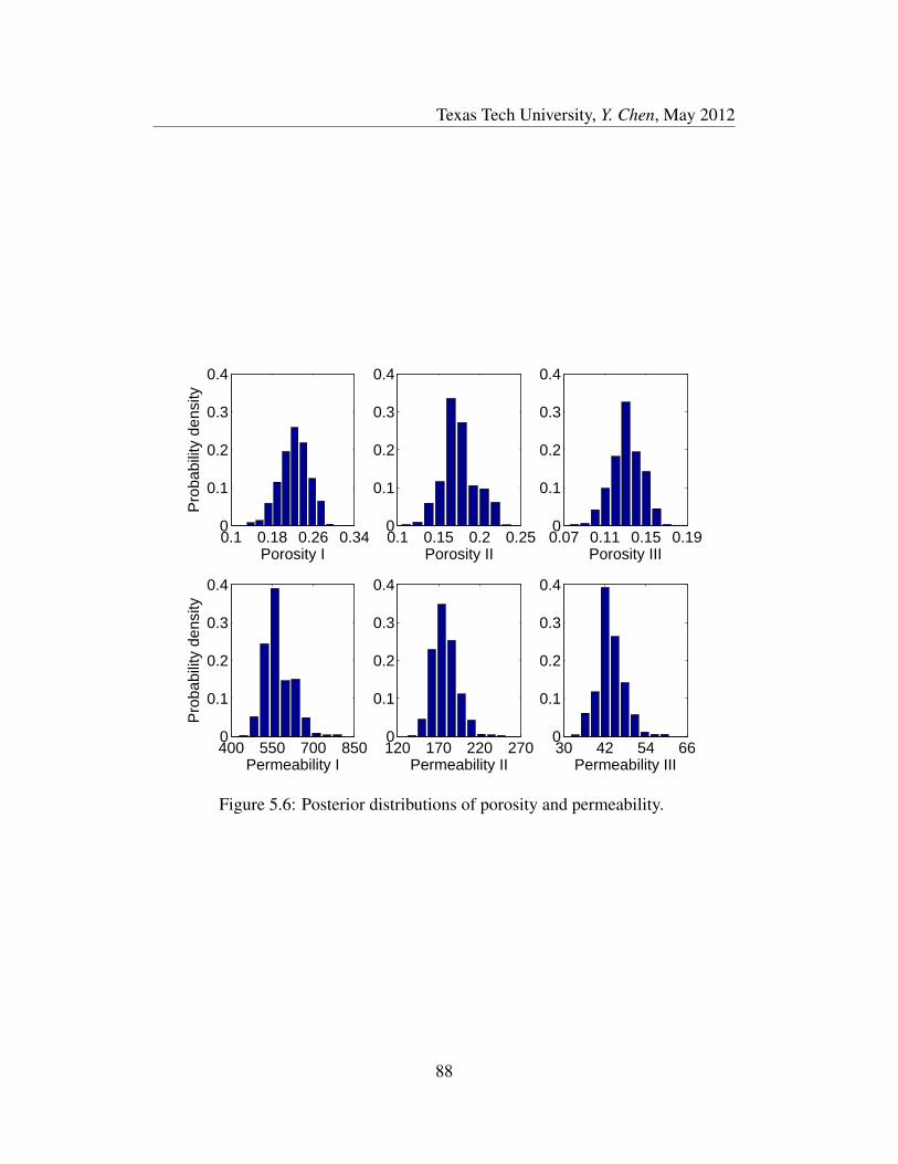
Texas Tech University, Y. Chen, May 2012
0.1 0.18 0.26 0.340
0.1
0.2
0.3
0.4
Porosity I
Pro
babi
lity
dens
ity
0.1 0.15 0.2 0.250
0.1
0.2
0.3
0.4
Porosity II0.07 0.11 0.15 0.190
0.1
0.2
0.3
0.4
Porosity III
400 550 700 8500
0.1
0.2
0.3
0.4
Permeability I
Pro
babi
lity
dens
ity
120 170 220 2700
0.1
0.2
0.3
0.4
Permeability II30 42 54 660
0.1
0.2
0.3
0.4
Permeability III
Figure 5.6: Posterior distributions of porosity and permeability.
88

Texas Tech University, Y. Chen, May 2012
True
50100
150
200
250
300
350
400
450
500
550
Initi
al
30 d
ays
120
days
180
days
240
days
300
days
390
days
Figu
re5.
7:In
itial
,tru
ean
dup
date
dpe
rmea
bilit
yof
rese
rvoi
r.
89
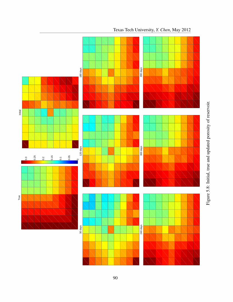
Texas Tech University, Y. Chen, May 2012
True
00.05
0.1
0.15
0.2
0.25
0.3
Initi
al
30 d
ays
120
days
180
days
240
days
300
days
390
days
Figu
re5.
8:In
itial
,tru
ean
dup
date
dpo
rosi
tyof
rese
rvoi
r.
90
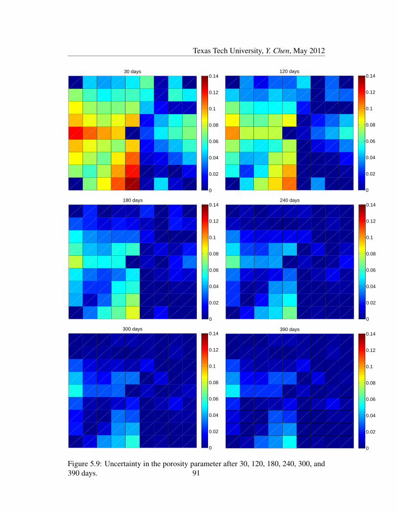
Texas Tech University, Y. Chen, May 2012
30 days
0
0.02
0.04
0.06
0.08
0.1
0.12
0.14120 days
0
0.02
0.04
0.06
0.08
0.1
0.12
0.14
180 days
0
0.02
0.04
0.06
0.08
0.1
0.12
0.14240 days
0
0.02
0.04
0.06
0.08
0.1
0.12
0.14
300 days
0
0.02
0.04
0.06
0.08
0.1
0.12
0.14390 days
0
0.02
0.04
0.06
0.08
0.1
0.12
0.14
Figure 5.9: Uncertainty in the porosity parameter after 30, 120, 180, 240, 300, and390 days. 91
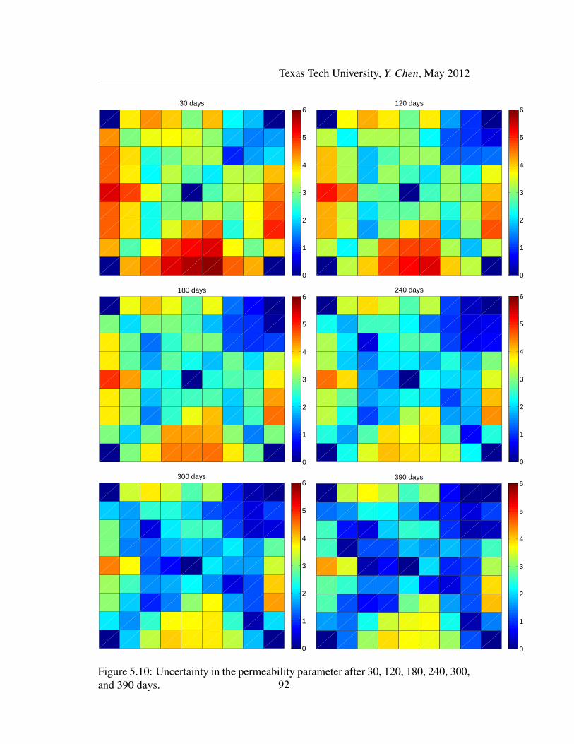
Texas Tech University, Y. Chen, May 2012
30 days
0
1
2
3
4
5
6120 days
0
1
2
3
4
5
6
180 days
0
1
2
3
4
5
6240 days
0
1
2
3
4
5
6
300 days
0
1
2
3
4
5
6390 days
0
1
2
3
4
5
6
Figure 5.10: Uncertainty in the permeability parameter after 30, 120, 180, 240, 300,and 390 days. 92
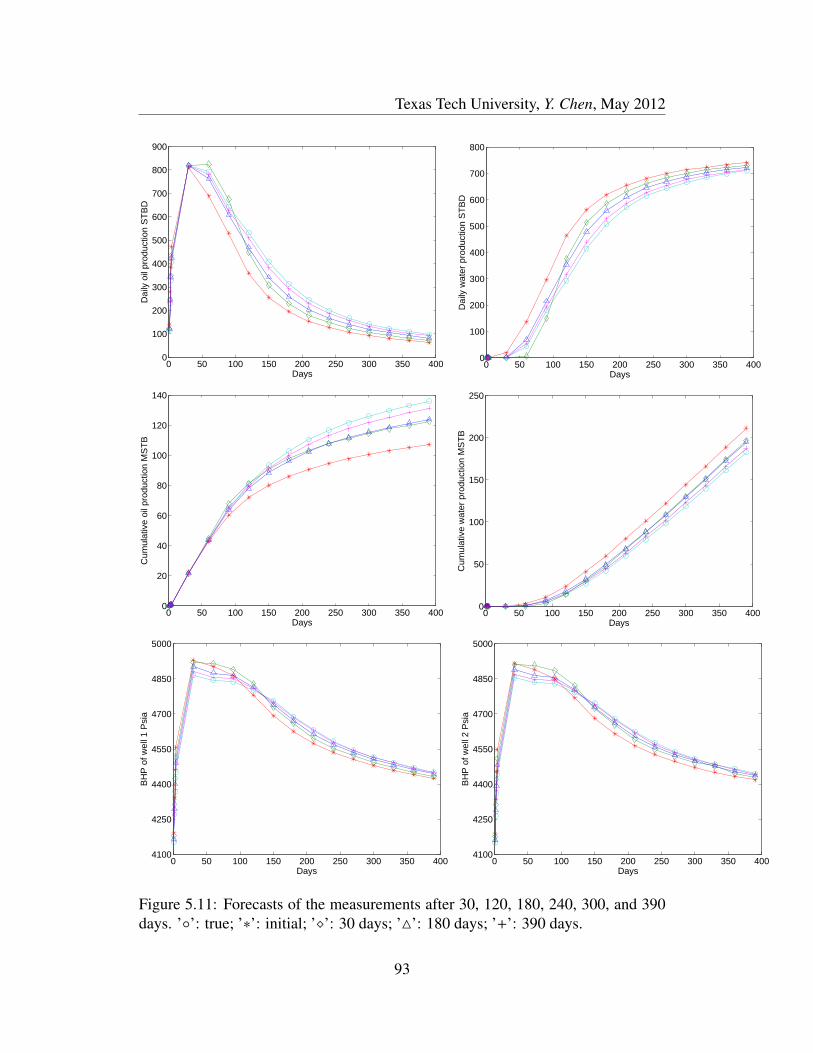
Texas Tech University, Y. Chen, May 2012
0 50 100 150 200 250 300 350 4000
100
200
300
400
500
600
700
800
900
Days
Dai
ly o
il pr
oduc
tion
STB
D
0 50 100 150 200 250 300 350 4000
100
200
300
400
500
600
700
800
Days
Dai
ly w
ater
pro
duct
ion
STB
D
0 50 100 150 200 250 300 350 4000
20
40
60
80
100
120
140
Days
Cum
ulat
ive
oil p
rodu
ctio
n M
STB
0 50 100 150 200 250 300 350 4000
50
100
150
200
250
Days
Cum
ulat
ive
wat
er p
rodu
ctio
n M
STB
0 50 100 150 200 250 300 350 4004100
4250
4400
4550
4700
4850
5000
Days
BH
P o
f wel
l 1 P
sia
0 50 100 150 200 250 300 350 4004100
4250
4400
4550
4700
4850
5000
Days
BH
P o
f wel
l 2 P
sia
Figure 5.11: Forecasts of the measurements after 30, 120, 180, 240, 300, and 390days. ’’: true; ’∗’: initial; ’’: 30 days; ’4’: 180 days; ’+’: 390 days.
93
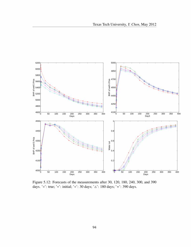
Texas Tech University, Y. Chen, May 2012
0 50 100 150 200 250 300 350 4004600
4800
5000
5200
5400
5600
5800
6000
6200
Days
BH
P o
f wel
l 3 P
sia
0 50 100 150 200 250 300 350 4004100
4250
4400
4550
4700
4850
5000
Day3
BH
P o
f wel
l 4 P
sia
0 50 100 150 200 250 300 350 4004050
4150
4250
4350
4450
4550
Days
BH
P o
f wel
l 5 P
sia
0 50 100 150 200 250 300 350 4000
0.2
0.4
0.6
0.8
1
Days
Wat
er c
ut
Figure 5.12: Forecasts of the measurements after 30, 120, 180, 240, 300, and 390days. ’’: true; ’∗’: initial; ’’: 30 days; ’4’: 180 days; ’+’: 390 days.
94
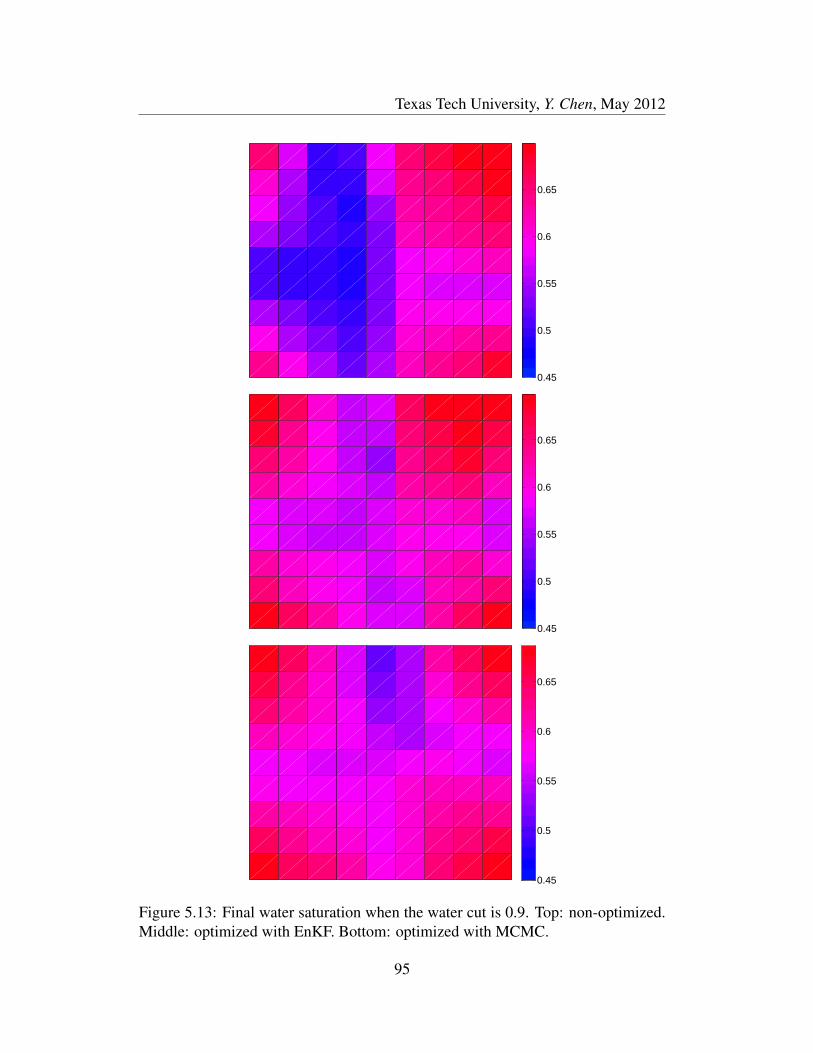
Texas Tech University, Y. Chen, May 2012
0.45
0.5
0.55
0.6
0.65
0.45
0.5
0.55
0.6
0.65
0.45
0.5
0.55
0.6
0.65
Figure 5.13: Final water saturation when the water cut is 0.9. Top: non-optimized.Middle: optimized with EnKF. Bottom: optimized with MCMC.
95

Texas Tech University, Y. Chen, May 2012
0 30 60 90 120 150 180 210 240 270 300 330 360 3900
40
80
120
160
200
Time (days)
Cum
ulat
ive
prod
uctio
n (M
STB
)
30 60 90 120 150 180 210 240 270 300 330 360 3900
2000
4000
6000
8000
10000
12000
14000
Time (days)
Cum
ulat
ive
NP
V (t
hous
and
dolla
rs)
Figure 5.14: Top: Comparison of cumulative production of oil and water. Opti-mized case: EnKF, oil () and water (5) production; MCMC, oil (+) and water(4) production. Non-optimized case: oil () and (∗): water production. Bottom:Cumulative NPV. Optimized: EnKF, blue; MCMC, green. Non-optimized: red.
96

Texas Tech University, Y. Chen, May 2012
05
1015
280300
320340
3600.1
0.15
0.2
0.25
0.3
StepsPermeability
Dim
ensi
onle
ss w
ater
flow
rate
05
1015
0.2
0.25
0.30.1
0.15
0.2
0.25
0.3
StepsPorosity
Dim
ensi
onle
ss w
ater
flow
rate
Figure 5.15: Optimal dimensionless injected water flow rate in the first well asa function of the updating steps, and the average permeability (top) and porosity(bottom) values.
97

Texas Tech University, Y. Chen, May 2012
05
1015
180200
220240
2600.1
0.15
0.2
0.25
0.3
StepsPermeability
Dim
ensi
onle
ss w
ater
flow
rate
05
1015
0.12
0.14
0.16
0.180.1
0.15
0.2
0.25
0.3
StepsPorosity
Dim
ensi
onle
ss w
ater
flow
rate
Figure 5.16: Optimal dimensionless injection water flow rate in the second well as afunction of the updating steps and average permeability (top) and porosity (bottom)values.
98

Texas Tech University, Y. Chen, May 2012
05
1015
200
220
240
2600.1
0.15
0.2
0.25
0.3
StepsPermeability
Dim
ensi
onle
ss w
ater
flow
rate
05
1015
0.2
0.25
0.30.1
0.15
0.2
0.25
0.3
StepsPorosity
Dim
ensi
onle
ss w
ater
flow
rate
Figure 5.17: Optimal dimensionless injection water flow rate in the third well as afunction of the updating steps and average permeability (top) and porosity (bottom)values.
99

Texas Tech University, Y. Chen, May 2012
05
1015
20
25
30
350.1
0.15
0.2
0.25
0.3
Dim
ensi
onle
ss w
ater
flow
rate
StepsPermeability
05
1015
0.06
0.08
0.1
0.120.1
0.15
0.2
0.25
0.3
Dim
ensi
onle
ss w
ater
flow
rate
StepsPorosity
Figure 5.18: Optimal dimensionless injection water flow rate in the fourth well as afunction of the updating steps and average permeability (top) and porosity (bottom)values.
100

Texas Tech University, Y. Chen, May 2012
Nomenclature
ARMA autoregressive moving average
BHP bottom hole pressure
EEF empirical eigenfunction
EnKF ensemble Kalman filter
MCMC Markov chain Monte Carlo
NPV net present value
ROM reduced-order model
A coeff matrix of water injection rates B coeff matrix of productionD(n) disturbance N total number of optimization stepsNprod number of produce well
a discounting factor d model outpute error term k absolute permeabilitykd time delay kr relative permeabilityl permeability correlation length n optimization stepsd scaling parameter t timeu water injection rates u(n) input at time step ny oil and water production φ porosity
Nlog log-normal distribution N normal distribution
101
Texas Tech University, Y. Chen, May 2012
Chapter 6
Robust Estimates of the Uncertain Parameters
As described in Chapter 4, when the parameters in a model are totally unknown,
to obtain the accurate estimates of process behavior from the model, it is necessary
to update the uncertain model parameters from measurements. However, updating
is a time consuming process. Once we have some information about the uncertain
parameter values, it is reasonable to use these values to generate a statistical esti-
mate based on some formal arguments. Traditionally, the mean value of the data
samples is used as a statistical estimate. However, considering the existence of out-
liers, insufficient sample size, and so forth, the statistical mean value may not the
best statistical estimate. In light of this argument, this chapter presents an overview
of the theory of robust statistics to provide a formal basis for the generation of a
statistical estimate. Based on robust statistics, a new theorem about a maximum
likelihood model parameterized by a maximum likelihood estimate of the uncer-
tain parameters is introduced and a formal proof of its existence is provided. The
contents of this chapter are excerpted from [5].
102

Texas Tech University, Y. Chen, May 2012
6.1 Robust Statistics Estimates
Given an uncertain parameter in a model, without loss of generality, it is fair
to assume that its values are constrained to be within a well-defined feasible range.
It is important to discuss how to choose a value from within this range because a
good estimate of this parameter may have a strong relationship to the real items of
interest, the estimates of the process states (i.e, the model outputs).
There are essentially three types of robust statistic methods to obtain a satisfac-
tory choice of the parameter value from its uncertain data set [39]. Assume X is an
uncertain variable with N possible values xi ∈ X : x1, x2, · · · , xN
1. Maximum likelihood estimate — MLE.
Let xM be an estimate of X. If xM is such that for any arbitrary function F,∑F(xi; xM) is minimum, then xM is the maximum likelihood estimate of X.
To obtain a value of xM, take the derivative of F with respect to xM and let∑ ∂F(xi; xM)∂xM
= 0.
2. Linear combination of order statistics — L-estimate.
L-estimates include the mean, trimmed mean, minimum and maximum val-
ues, and so forth.
3. Rank test estimate — R-estimate
For a variable X with samples xi, i = 1, 2, · · · ,N, if an estimate xR can make
103
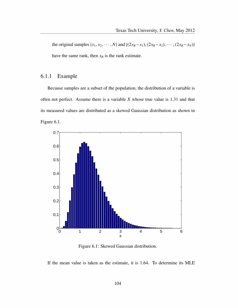
Texas Tech University, Y. Chen, May 2012
the original samples x1, x2, · · · ,N and (2xR−x1), (2xR−x2), · · · , (2xR−xN)
have the same rank, then xR is the rank estimate.
6.1.1 Example
Because samples are a subset of the population, the distribution of a variable is
often not perfect. Assume there is a variable X whose true value is 1.31 and that
its measured values are distributed as a skewed Gaussian distribution as shown in
Figure 6.1.
0 1 2 3 4 5 60
0.1
0.2
0.3
0.4
0.5
0.6
0.7
x
Figure 6.1: Skewed Gaussian distribution.
If the mean value is taken as the estimate, it is 1.64. To determine its MLE
104

Texas Tech University, Y. Chen, May 2012
value, let F(xi; xM) = |xi − xM |. Thus, xM is the median of the measurements. To
obtain its L-estimate, assume a 20% trimmed mean. Discard 10% of the ordered
samples at the bottom and the top of the samples. By so doing the L-estimate is
1.57. To find the R-estimate, apply the Wilcoxon rank test.
Table 6.1 lists the MLE, L-estimate, R-estimate and the errors between these
estimates and the true value. From this simple example and the data in the table,
we can determine that the MLE value is closest to the true value for this skewed
Gaussian distribution. We also note that the mean value has the largest error. We
may conclude with some confidence that robust statistics can be used to provide a
better estimate.
Table 6.1: Estimates and errors
xM xL xR mean
value 1.40 1.57 1.47 1.64
errors 0.09 0.26 0.16 0.33
6.2 Preamble
Although robust statistics can provide satisfactory choices of the values of the
uncertain parameters, these estimates are dependent on the feasible parameter ranges
and the choice of their distribution. Usually a process model contains more than one
parameter that the model outputs are sensitive to. The propagated combinations of
105

Texas Tech University, Y. Chen, May 2012
the samples of these parameters through the model must satisfy the constraints of
the state variables.
Definition 6.1. Parameter uncertainty
If a model parameter P j, j = 1, · · · ,m has more than one value: p1j , p
2j , · · · , p
nj .
Then, this set reflects the uncertainty of P j.
Remark 6.1. A parameter is uncertain if the parameter can have more than one
value.
Definition 6.2. Model parametrization,M
Let FM be a space of operators and FM ⊂ FM , Ø. Here FM can be linear or
nonlinear time-varying operators. We define a model based on a parameter set by
M (p) = fM(p)
where fM ∈FM.
Remark 6.2. A model is complete if the model parameters P j, j = 1, · · · ,m are all
assigned values.
Definition 6.3. Evaluation models,M (P )
Let P be a set of evaluation model parameters andM be a model parametriza-
tion. The set of evaluation models is
M (P ) = M (p)
where p are values assigned to P
106

Texas Tech University, Y. Chen, May 2012
Definition 6.4. State estimates, y
Let P be a set of evaluation model parameters andM be a model parametriza-
tion M (P ). The set of state estimates, y ∈ Rk, is a solution of the evaluation
models, y = M (p), where p are values assigned to P .
Remark 6.3. The set of evaluation model parameters P and the set of sensitive
model parameters Ps is distinguished; Ps ⊆ P . Let Pn be the set of non-sensitive
parameters, Pn ⊂ P . Thus, Ps ∪ Pn = P and
∣∣∣∣∣ ∂y∂Ps
∣∣∣∣∣ ∣∣∣∣∣ ∂y∂Pn
∣∣∣∣∣Remark 6.4. Since Ps ⊆ P , thenM (Ps) ⊆M (P ).
Definition 6.5. Plant measurements, yM
Let yM : yM,`, ` = 1, · · · , nm be a set of plant measurements,
Remark 6.5. The target values y∗M are assumed to be stable equilibrium states of
the plant but constrained
y∗M − δyl ≤ yM ≤ y
∗M + δy
u, δyl ≥ 0, δyu ≥ 0.
In the case of the ideal plant, yP ≡ y∗M.
Remark 6.6. The set of disturbances (measured or unmeasured) is denoted by d.
The true outputs of the plant (unaffected by disturbances) yP is related to the mea-
sured values by, yM = yP + d.
107

Texas Tech University, Y. Chen, May 2012
Remark 6.7. y = M (p). The outputs of the model should be close to that of the
outputs of the undisturbed plant yP when perturbed by the same inputs,
‖ yP − y ‖2=‖ ε ‖2≤ ε0
Definition 6.6. Set of models with sensitive parameters,M (Ps)
Let Ps be a set of sensitive model parameters andM be a model parameterized
by Ps,
M (Ps) = M (ps)
where ps are the values assigned to Ps
Remark 6.8. The setM (Ps) will be used to determine feasible combinations of Ps
constrained by the range of the plant measurements yM. Because the set Pn has
negligible effects on y, the values assigned to the members of the set Pn are fixed
at their nominal values and are not considered when determining feasible combi-
nations of Ps. For simplicity, in the development that follows, the term ’uncertain
parameters’ means ’sensitive uncertain parameters’.
Definition 6.7. Feasible ranges of ps, [pls,p
us]
Let ps be a set of the values of Ps in the feasible ranges, [pls,p
us], and M be a
model parametrization such that y = M (ps). The feasible ranges satisfy
y∗M − δyl ≤ y ≤ y∗M + δy
u
108

Texas Tech University, Y. Chen, May 2012
Definition 6.8. Robust estimates of model uncertain parameters, ps
Let [pls,p
us] be the feasible range of the uncertain parameter andM be a model
parametrization. State estimates, y, determined by a model parameterized by the
robust estimates are closer to the states from the actual plant than state estimates
found from a model parameterized by anything other the robust parameter estimates
‖ yP − y ‖2 = ‖ yP − M (Ps) ‖2 = ε
‖ yP − y ‖2 = ‖ yP − M (Ps) ‖2 = ε ≤ ε
Remark 6.9. Robust estimates of the uncertain parameters must be within their
feasible ranges, pls ≤ ps ≤ p
us .
Definition 6.9. Errors, e
The set of errors is the difference between the measured values and the model’s
estimates,
e = yM − y
Remark 6.10. Since disturbance may not be measurable, the error between the
model and the measurement is one means of estimating the disturbance,
‖ d − e ‖2 = εd
Definition 6.10. Model-based controller operator, C(M , e)
Let FC be a non-empty space of operators and FC ⊂ FC. A model-based con-
troller operator is defined as
109
Texas Tech University, Y. Chen, May 2012
C := FM × e→ FC : (M , e) 7→ fC = C(M , e)
where fC ∈ FC. The absence of a controller is given by, e : fC = 0
Definition 6.11. Model-based controller outputs, U
According to the target values, y∗M, the controller outputs are the solution of
C(M , e) that forces the measured values ym to follow the trajectory of y∗M in finite
time, T .
U = C(M , e) × y∗M : limt→t+T
yM → y∗M
Remark 6.11. The model-based controller outputs, U , can provide compensation
in the face of disturbances,
limt→t+TU × P = yP − e + d = y
∗M + d − e = y
∗M + εd
where P represents the actual plant.
Definition 6.12. Nominal model,MN
The nominal model MN is a model whose parameter values are the designed
nominal values.
Definition 6.13. Maximum likelihood model, M
A maximum likelihood model can provide robust estimates of the disturbances
such that compensation from the maximum likelihood model-based controller makes
110

Texas Tech University, Y. Chen, May 2012
the errors between the measurements and the targets smaller than any other model-
based design controller.
‖ yP − M ‖2 ≤ ‖ yP −MN ‖2
dn = yM −MN d = yM − M
‖ d − dn ‖2= εd ‖ d − d ‖2= εd ≤ εd
From definition 6.9 and remark 6.10,
en = yM − y = yM −MN = dn
e = yM − y = yM − M = d
Let U and andUN be controller outputs based on a maximum likelihood model-
based controller design and a nominal model-based controller design, respectively
U = C(M , e) × y∗M
UN = C(MN , en) × y∗M
The compensation determined by the nominal model-based controller design
results in
limt→t+T
y∗M − yM = y∗M − UN × P = y
∗M − (yP − en + d) = εd
In contrast, the compensation determined by the maximum likelihood model-
111

Texas Tech University, Y. Chen, May 2012
based controller design results in
limt→t+T
y∗M − yM = y∗M − U × P = y
∗M − (yP − e + d) = εd ≤ εd
6.3 Mathematical Foundation
Lemma 6.1. The feasible ranges of the uncertain parameters are distribution inde-
pendent.
Proof: Assume ps ∈ [pLs ,p
Us ] and the feasible ranges [pl
s,pus] ⊆ [pL
s ,pUs ]. From
the preamble, [y∗ − δyl,y∗ − δyu]′ = M (pls,p
us). Since the values of pl
s and pus
are distribution independent, it follows that the feasible ranges also are distribution
independent. QED
Lemma 6.2. The distributions of the set of uncertain parameters affect their robust
estimates according to the constraints imposed by the real plant.
Proof: There are two cases.
1. Uniqueness. There is only one combination of parameter values, pos , such that
y =M (pos) ∈ [y∗ − δyl,y∗ + δyu]. In this case, the value of each uncertain
parameter is the robust estimate of the model parametrization that gives the
smallest error.
2. More than one combination of the uncertain parameter values in the feasible
range, pls ≤ ps ≤ p
us , are admissible and satisfy y =M (ps) ∈ [y∗ − δyl,y∗ +
112

Texas Tech University, Y. Chen, May 2012
δyu].
Different distributions of the uncertain parameter values will give different
values of P
P(a ≤ ps ≤ b) =∫ b
apd f (ps) dps
where pd f is the probability density function of an uncertain parameter.
Different distributions of the uncertain parameters will give different values
of P(ps).
The uncertain values ps ∈ [pls, p
us] of the parameters must satisfy their fea-
sible range (see lemma 6.1). Clearly, each assigned distribution may yield a
different probability value as a potential estimate of the value of the uncertain
parameter. Therefore, the assigned distributions of the uncertain parameters
will affect their robust estimates. QED
Theorem 6.1. A model parameterized with robust estimates of the uncertain pa-
rameters is the maximum likelihood model,M (ps) = M .
Proof: Assume y =M (ps) and y =M (ps).
From definition 6.8,
‖ yP − y ‖2 = ‖ yP −M (Ps) ‖2 = ε
‖ yP − y ‖2 = ‖ yP −M (Ps) ‖2 = ε ≤ ε
113

Texas Tech University, Y. Chen, May 2012
Estimates of the disturbances obtained from MN = M (ps) are given by (see
remark 6.6),
‖ d − dN ‖2 =‖ d − (yM − y) ‖2
=‖ d − yM + yP − ε ‖2
‖ d − dN ‖2 =‖ d − d − ε ‖2= ε
For the nominal model parametrization,M (ps),
limt→t+T
y∗M − yM = ε
Estimates of disturbances obtained fromM (ps),
‖ d − d ‖2 =‖ d − (yM − y) ‖2
=‖ d − yM + yP − ε ‖2
=‖ d − d − ε ‖2
‖ d − d ‖2 = ε ≤ ε
For the robust estimate parametrization,M (ps),
limt→t+T
y∗M − yM = ε ≤ ε
This means that M (ps) can provide estimates of the disturbances such that
the compensation from this model-based controller design makes the plant outputs
114

Texas Tech University, Y. Chen, May 2012
track their target values with less offset than one based on M (ps). It then follows
thatM (ps) = M . QED
Lemma 6.3. The estimates y obtained from the maximum likelihood Model, M ,
are closer to the real plant estimates yP than those obtained from any other model
parametrization.
Proof: According to definition 6.13,
‖ d − (yM − y) ‖2= ε
‖ d − (yM − y) ‖2= εd ≤ ε
However,
‖ y − yP ‖2 = ‖ y + d − (yP + d) ‖2
= ‖ d − (yM − y) ‖2
‖ y − yP ‖2 = ε
and
‖ y − yP ‖2 = ‖ y + d − (yP + d) ‖2
= ‖ d − (yM − y) ‖2
‖ y − yP ‖2 = εd ≤ ε
QED
Lemma 6.4. The error between the target values, y∗M, and the plant measurements
forced by U , the outputs of a maximum likelihood model-based controller design is
115

Texas Tech University, Y. Chen, May 2012
smaller than the error between y∗M and the plant measurements forced by Un from
any other model-based controller design.
Proof: For a nominal model-based controller design (see definition 6.11 and remark
6.11),
limt→t+T
(y∗M −Un × P)′(y∗M −UN × P) = ε′dεd
For a maximum likelihood model-based controller design,
limt→t+T (y∗M − U × P)′(y∗M − U × P) = ε′dεd
εd ≤ εd
ε′dεd ≤ ε′dεd
QED
6.3.1 Example
There are two cases, linear and nonlinear models. Assume both linear and non-
linear models have two uncertain parameters P j, j = 1, 2. The uncertain original
ranges are 1 ≤ P1 ≤ 12, 11 ≤ P2 ≤ 20. The constraint on the model output is
14 ≤ y ≤ 22. The largest feasible ranges for all uncertain parameters should be
considered together.
Case 1: the model is a linear combination of parameters, M(P ) : y =2∑
j=1P j.
• Assume P j2j=1 are uniformly distributed, that is, P1 ∼ U (1, 10), P2 ∼
116

Texas Tech University, Y. Chen, May 2012
U (11, 20). There are more than one feasible combination of uncertain pa-
rameters that satisfy the constraint on y:1
13
≤
P1
P2
≤
2
20
,
3
11
≤
P1
P2
≤
12
14
,2
12
≤
P1
P2
≤
6
16
, · · ·• P j
2j=1 are normally distributed. P1 ∼ N (5.5, 1.44), P2 ∼ N (15.5, 1.44).
Sample N points for each parameter in their original ranges. the number of
sample points for each parameter can be chosen according to the efficiency of the
sampling techniques [18, 19]. In this example, the feasible ranges of P j2j=1 are
2 ≤ P1 ≤ 6, 12 ≤ P2 ≤ 16. After the feasible ranges of the uncertain parameters are
determined, the samples are used to calculate the robust estimates.
M –, L –, and R – robust estimates of P j2j=1 are listed in Table 6.2. In these
estimates, the function F(xi; xM) = |xi − xM | is used to find the M-estimate); the
mean value is used for an L-estimate; and the Wilcoxon test is use to obtain an
R-estimate.
Case 2: the model is nonlinear, M(P ) : y = exp(P1) + P2.
The feasible ranges for P j2j=1 are 1 ≤ P1 ≤ 2, 11.3 ≤ P2 ≤ 14.7.
• Uniform distributions, P1 ∼ U (1, 10), P2 ∼ U (11, 20)
• Normal distributions, P1 ∼ N (5.5, 1.44), P2 ∼ N (15.5, 1.44).
117

Texas Tech University, Y. Chen, May 2012
Table 6.2: Robust estimates. y =2∑
j=1P j.
Uniform Normal
Estimate M±1.155 L±1.155 R±1.155 M±0.757 L±0.748 R±0.750
P1 4 4 4 5.04 4.92 4.97
P2 14 14 14 15.04 14.92 14.97
Robust estimates of P j2j=1 are listed in Table 6.3. Robust estimates of the
uncertain parameters are both distribution and model-type dependent (see lemma
6.2).
Table 6.3: Robust estimates. y = exp(P1) + P2
Uniform
Estimate M±σ L±σ R±σ
P1 1.5±0.289 1.5±0.289 1.5±0.289
P2 13±0.9815 13±0.9815 13±0.9815Normal
Estimate M±σ L±σ R±σ
P1 1.79±0.2226 1.74±0.2231 1.76±0.2177
P2 14.19±0.543 14.06±0.528 14.12±0.531
From this example, Lemma 6.2 is further proven. The robust estimates of the
uncertain parameters are both distributions and model-type dependent.
6.4 Summary
Robust statistics is introduced in this chapter to obtain robust estimates of the
uncertain parameters from their samples. A theorem is developed and proven to
118
Texas Tech University, Y. Chen, May 2012
show that the model parameterized with robust estimates of the uncertain param-
eters is the maximum likelihood model. This model then can be employed to ob-
tain robust estimates of disturbances and states of the plant. Thus, the maximum
likelihood model can improve the performance of model-based applications when
compared to the nominal model-based applications.
119

Texas Tech University, Y. Chen, May 2012
Nomenclature
MLE maximum likelihood estimation
pd f probability density function
L-estimation linear estimation
R-estimation rank estimation
C model-based controller M model parametrizationP parameters Pn non-sensitive parametersPs sensitive parameters U controller outputsX uncertain variabled disturbances e errorxL linear estimate xM maximum likelihood estimatexR rank estimate y state estimates from modelyM plant measurements y∗M target valuesyp plant state without disturbances N normal distributionU uniform distribution
120
Texas Tech University, Y. Chen, May 2012
Chapter 7
State Estimation & Model Predictive Control with a Max-
imum Likelihood Model
Based on the knowledge of robust statistics and consideration of state variable
constraints, a maximum likelihood model which is parameterized with the robust
estimates of model uncertain parameters was introduced in Chapter 6. This chap-
ter demonstrates the robustness features of the maximum likelihood model (MLM)
namely, accurate state estimation and improve the model-based application per-
formance, in a model predictive control (MPC) framework1. The content of this
chapter is excerpted from [5].
7.1 Tubular Reactor
To demonstrate the performance of the MLM in a real-time application that in-
volves state estimation and optimal control, a chemical reaction that occurs in a
tubular reactor is introduced [4]. A dimensionless first-principles model that de-
1The concepts of model-based control and MPC are reviewed in Appendix A.
121

Texas Tech University, Y. Chen, May 2012
scribes this reaction is given by,
∂T∂t=
1Peh
∂2T∂z2 −
1Le∂T∂z+ ηCeγ(1−1/T ) + µ[Tw(z, t) − T (z, t)]
∂C∂t=
1Pem
∂2C∂z2 −
∂C∂z− DaCeγ(1−1/T )
(7.1)
The boundary conditions are:
z = 0
∂T∂z= Peh(T (z, t) − Ti(t))
∂C∂z= PeM(C(z, t) −Ci(t))
z = 1
∂T∂z= 0
∂C∂z= 0
The state variables T and C are dimensionless temperature and concentration,
respectively. The dimensionless wall temperature Tw is regulated to control the
reaction temperature by changing the flow rate of the cooling fluid. The reference
temperature is 500C. The parameters values for the fluid are listed in Table 7.1.
In this reactor model, the outputs are found to be most sensitive to Peh, η, and
µ. A 10% change in Peh and η will increase the reactor temperature by 2.9% and
1.8%, respectively; and a 10% increase in µ will decrease reactor temperature by
1.5%. Assume they are the uncertain parameters and that their distributions are Peh
– U (4, 6), η – N (0.84, 0.007) and µ – Nlog(log(12.6), 1.3).
122

Texas Tech University, Y. Chen, May 2012
Table 7.1: Dimensionless parameters for the tubular reactor [4].Parameter Nominal value Definition
Peh 5.0 Heat Peclet number
Pem 5.0 Mass Peclet number
Le 1.0 Lewis number
Da 0.875 Damkohler number
γ 15.0 Activation energy
η 0.8375 Heat of reaction
µ 13.0 Heat transfer coefficient
Tw(z, 0) 1.0 Dimensionless wall temperature
Ti(0) 1.0 Dimensionless inlet temperature
Ci(0) 1.0 Dimensionless inlet concentration
7.2 Determination of Robust Estimation of Uncertain Parameters
for State Estimation
According to lemma 6.3 in Chapter 6, the MLM can provide more accurate
estimates than the nominal model. Moreover, in the absence of disturbances, the
errors between the MLM estimates and the actual plant measurements, yM, will be
the smallest.
In the present case, one of the state variables, concentration, is not measured as
frequently as the other. To circumvent this sparseness, the first-principles model can
be used to provide in silico data to develop the partial least squares (PLS) regression
model. An important issue is how to determine the feasible ranges of the uncertain
123

Texas Tech University, Y. Chen, May 2012
parameters to enable calculation of the robust estimates. In this application of open-
loop state estimation of the reactor, a threshold value of three times the standard
deviation (this value can be determined from the historical data) of the measured
plant values is selected to develop the PLS model, the outputs yPLS ∈ [yM−3σ,yM+
3σ].
Measurements from the plant will be compared to the state estimates from the
PLS model. If the absolute errors between them are within ±3σ, ‖ yM − yPLS ‖2≤
3σ, the values assigned to the uncertain parameters are assumed to be the correct
robust estimates. Otherwise, the feasible ranges are revised, as shown in Figure
7.1. This revision can be accomplished by sampling the uncertain parameter dis-
tributions and propagating the sampled values through the first-principles model.
The sets of parameter values giving y ∈ [yM − 3σ,yM + 3σ] determine the feasible
ranges. Based on the work in Chapter 2, the Latin hypercube Hammersley sampling
(LHHS) technique is used since it is known to be very efficient when sampling mul-
tiple uncertain parameter distributions.
PlantInput
)ˆ(ˆ Θ= MM PLS modely PLSy
My
+-
σ3|| >eLHHS
updateΘ
Figure 7.1: State estimation framework with a maximum likelihood model.
124

Texas Tech University, Y. Chen, May 2012
In the reactor example, the prediction variables to build PLS model are the reac-
tor feed and wall temperatures and the feed concentration. The response variables
are the reactor exit temperature and exit concentration.
When the feed reactor temperature decreases below the optimum reaction condi-
tions, the reactor exit temperature decreases, but the exiting reactant concentration
increases. This is because at a lower reaction temperature, less reactant is con-
verted. Figure 7.2 shows the change in the exiting temperature and concentration.
The top and bottom lines show the range of the state estimates from the PLS model
(yM ± 3σ). The plus-symbols (+) are the measured values from the real plant. The
circle-symbols () are the estimates from the PLS model developed using robust
parameter values.
From Figure 7.2 it is observed that the PLS state estimates are within the ±3σ
range after two updates of the uncertain parameter values. The exit temperature is
within the ±3σ range, but the exit concentration violates its threshold twice. This
violation triggers updating of the uncertain parameter values. Note, the concen-
tration graph does not show this violation clearly due to the size of the change,
which is over a wide range. Figure 7.3 more clearly shows the updates based on the
plant measurements. The diamond-symbol (q) represents the PLS state estimates
that violate the ±3σ range. Once the uncertain parameter values are updated, the
subsequent PLS state estimates are found to be within the ±3σ range.
Table 7.2 lists the nominal and updated uncertain parameter values. The robust
125
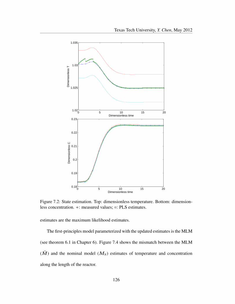
Texas Tech University, Y. Chen, May 2012
0 5 10 15 201.02
1.025
1.03
1.035
Dimensionless time
Dim
ensi
onle
ss T
0 5 10 15 200.18
0.19
0.2
0.21
0.22
0.23
Dimensionless time
Dim
ensi
onle
ss C
Figure 7.2: State estimation. Top: dimensionless temperature. Bottom: dimension-less concentration. +: measured values; : PLS estimates.
estimates are the maximum likelihood estimates.
The first-principles model parameterized with the updated estimates is the MLM
(see theorem 6.1 in Chapter 6). Figure 7.4 shows the mismatch between the MLM
(M ) and the nominal model (MN) estimates of temperature and concentration
along the length of the reactor.
126

Texas Tech University, Y. Chen, May 2012
0 1 2 3 40.182
0.184
0.186
0.188
0.19
0.192
0.194
0.196
Dimensionless time
Dim
ensi
onle
ss C
Figure 7.3: State estimation. Dimensionless concentration. +: plant measurements;: PLS estimates. q: PLS estimates that violate the ±3σ limits.
Table 7.2: Nominal values and robust estimates of the uncertain parameters
Peh η µ
Nominal Θ 5.0 0.8375 13.0
Robust Θ1 4.83 0.859 12.54
Robust Θ2 4.78 0.856 12.49
7.2.1 Maximum Likelihood Model for Model Predictive Control
Assume the robust estimates of the model uncertain parameters are as listed in
Table 7.2. Assume that a model, called the MLM, based on these robust estimates,
will be used in a MPC framework. Figure 7.5 shows the MPC framework with the
MLM.
Discrete linear time-invariant (DLTI) models have been used successfully in
many MPC applications. Bageshwar and Borrelli [75] proposed an offset-free MPC
127

Texas Tech University, Y. Chen, May 2012
0 0.2 0.4 0.6 0.8 11.02
1.03
1.04
1.05
1.06
1.07
1.08
1.09
1.1
1.11
Dimensionless length
Dim
ensi
onle
ss T
0 0.2 0.4 0.6 0.8 10.1
0.2
0.3
0.4
0.5
0.6
0.7
0.8
Dimensionless length
Dim
ensi
onle
ss C
Figure 7.4: Outputs of the nominal and maximum likelihood models. Top: dimen-sionless temperature. Bottom: dimensionless concentration. : states estimatesfrom M ; ∗: states estimates fromMN .
128
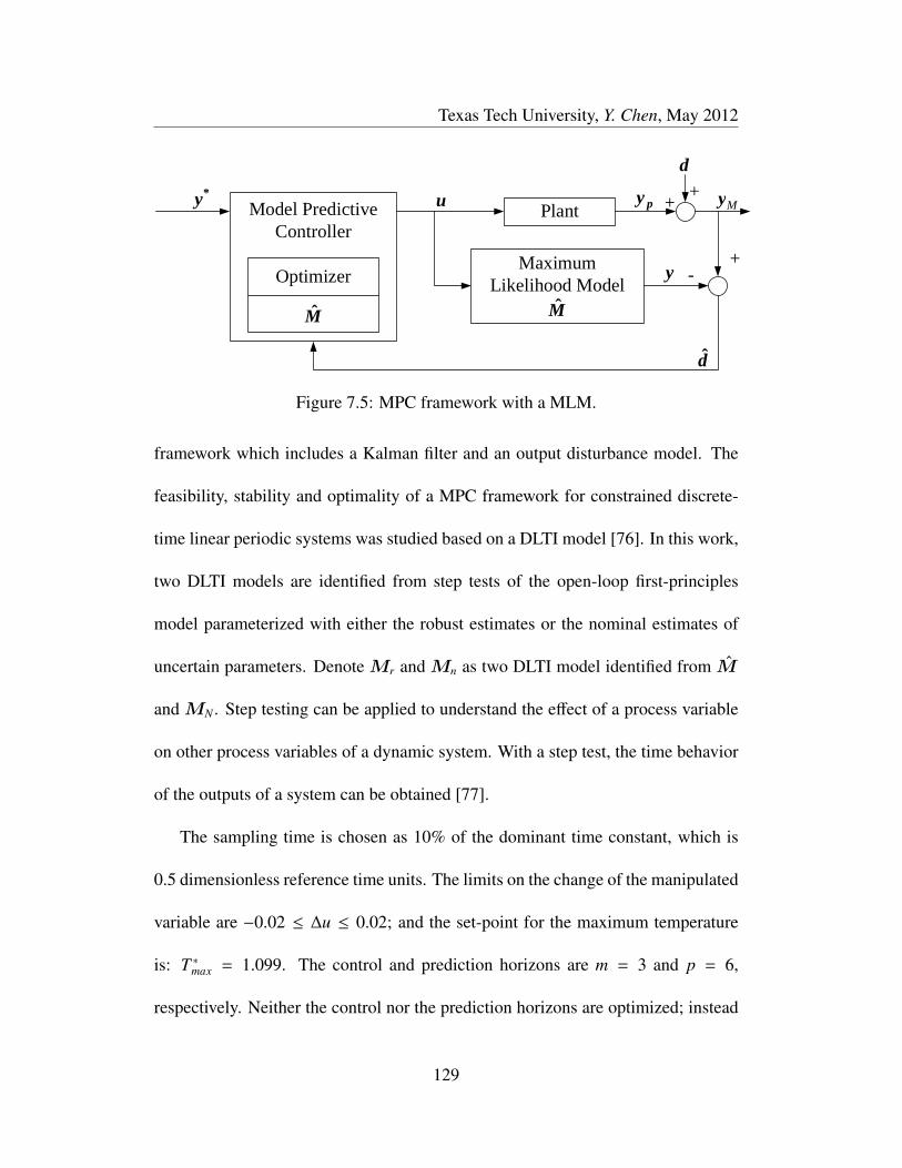
Texas Tech University, Y. Chen, May 2012
Model PredictiveController
Optimizer
M
Plant
MaximumLikelihood Model
M
py
d
my++
+-y
d
*y u
Model PredictiveController
Optimizer
M
Plant
MaximumLikelihood Model
M
py
d
My++
+-y
d
*y u
Figure 7.5: MPC framework with a MLM.
framework which includes a Kalman filter and an output disturbance model. The
feasibility, stability and optimality of a MPC framework for constrained discrete-
time linear periodic systems was studied based on a DLTI model [76]. In this work,
two DLTI models are identified from step tests of the open-loop first-principles
model parameterized with either the robust estimates or the nominal estimates of
uncertain parameters. Denote Mr and Mn as two DLTI model identified from M
and MN . Step testing can be applied to understand the effect of a process variable
on other process variables of a dynamic system. With a step test, the time behavior
of the outputs of a system can be obtained [77].
The sampling time is chosen as 10% of the dominant time constant, which is
0.5 dimensionless reference time units. The limits on the change of the manipulated
variable are −0.02 ≤ ∆u ≤ 0.02; and the set-point for the maximum temperature
is: T ∗max = 1.099. The control and prediction horizons are m = 3 and p = 6,
respectively. Neither the control nor the prediction horizons are optimized; instead
129
Texas Tech University, Y. Chen, May 2012
general rules are applied to arrive at these values.
To compare the closed-loop performance withMr– andMn– based controllers,
the following closed-loop performance criteria of the rise time, settling time, and
deviation from set-point are used[77].
Definition 7.1. Rise time: the first time the response reaches the set-point value
after a perturbation. A short rise time is often desired.
Definition 7.2. Settling time: the minimum time that the closed-loop response en-
ters and remains within a ±5% error band. A short settling time is usually favored.
Definition 7.3. Deviation from the set-point: the first peak value reached by the
closed-loop response. It also can be expressed as the percentage of the first peak
deviation of the closed-loop response from its set-point to its set-point value.
Random disturbances occur every 6 control steps; the disturbance is assumed
to be uniformly distributed, du ∈ [-0.01,0.01]. Figure 7.6 shows the closed-loop
performance with the MLE model, Mr, and the nominal model, Mn. For com-
parison, the disturbances are the same for both Mr– and Mn– based controllers.
From the figure, it can be observed that with the MLE-based controller, T reaches
its set-point with fewer control steps than withMn-based controller. Moreover, the
Mn-based controller output has more frequent changes.
Figures 7.7 and 7.8 show the closed-loop performance for the same disturbance
and also when the uncertain parameters’ values are decreased or increased by 3%,
130
Texas Tech University, Y. Chen, May 2012
respectively. The performance with either model-based controllers when the pa-
rameters’ values are decreased is similar with theMn-based controller response re-
quiring 3 more control steps to settle to the set-point value. The response has both
shorter rise and settling times; and the deviations from the set-point are smaller. We
can conclude that the Mr-based controller gives a better closed-loop performance
when the parameters’ values are increased.
To compare the errors between the set-point and the two model-based controller
responses, the integral of the time-weighted absolute error (ITAE) is calculated,
ITAE =∫ t
0t | e(t) | dt (7.2)
where t is time and e(t) is the error between the set-point and the closed-loop re-
sponse at time t.
Table 7.3 shows the ITAE and other controller performance criteria. In the
presence of the random unmeasured disturbances, theMr-based controller response
has smaller rise and settling times and set-point deviations. When the parameters’
values are decreased by 3%, theMr-based controller has a slightly longer rise time
but a much shorter settling time. When the parameters’ values are increased by
3%, the Mr-based controller response exhibits both shorter rise and settling times.
The set-point deviations also are smaller. In every case, the ITAE values associated
with the Mr-based controller are smaller than the ITAE values associated with the
131

Texas Tech University, Y. Chen, May 2012
Mn-based controller.
Table 7.3: Closed-loop performance comparison betweenMr andMn
Case Model ITAE Rise time Settling time Set-point dev(%)
random duMr 0.7407 1.8 1 1.7Mn 1.9530 2.8 3 2.4
∆Θ=-3%Mr 1.5204 3 1.6 2.2Mn 2.2610 2 6.8 2.2
∆Θ=+3%Mr 0.9815 2 0.4 1.5Mn 2.4677 4.5 2.5 2.4
Figure 7.9 shows the closed-loop performance when the set-point trajectory is
a stable first-order response. From the figure, it can be observed that both the Mr–
andMn– based controllers track the reactor temperature trajectory satisfactorily. In
the case of theMn-based controller, there is a small overshoot before settling to the
final value.
Figures 7.10 and 7.11 show the closed-loop controller performance when the
parameters’ values are decreased and increased by 3%, respectively. In the former
case, the Mn-based controller response shows more deviations from the set-point.
In the latter case, the reactor temperature response with the Mr-based controller
has a slightly larger overshoot from the set-point than the response with the Mn-
based controller. However, the rise and settling times are larger with theMn-based
controller and the changes in the manipulated variable are latched at the upper con-
straint.
132

Texas Tech University, Y. Chen, May 2012
Table 7.4 shows the ITAE and controller performance criteria when tracking a
first-order response in the presence of ±3% changes in the uncertain parameters’
values. In the case of set-point tracking, the Mr-based controller has smaller rise
and settling times and set-point deviations. When the values of the uncertain pa-
rameters are decreased by 3%, the Mr-based controller has a longer rise time but
a shorter settling time. The set-point deviations also are less. When the values of
the uncertain parameters are increased by 3%, the Mr-based controller has shorter
rise and settling times. In every case, the ITAE values associated with the Mr-
based controller are smaller than the ITAE values associated with the Mn-based
controller.
Table 7.4: Closed-loop performance comparison betweenMr andMn
Case Model IASE Rise time Settling time Set-point dev(%)
random duMr 0.1676 5.9 4 0.19Mn 0.2966 6.2 6 0.40
∆Θ=-3%Mr 0.2601 7 6 0.08Mn 0.5727 4.7 9 0.74
∆Θ=+3%Mr 0.2882 5 5 0.2Mn 0.4359 7 6 0.11
7.3 Summary
The maximum likelihood model is parameterized with robust estimates of the
uncertain parameters. To generate this model, the constraints imposed by the practi-
133

Texas Tech University, Y. Chen, May 2012
cal measurements must be considered to determine the feasible ranges of uncertain
parameters. Robust estimates of the uncertain parameters are calculated from the
feasible ranges using robust statistics theory. A maximum likelihood model was
developed for an example chemical reaction process and used in a model predictive
control framework to demonstrate its robust properties. It was found that accu-
rate state estimation resulted in satisfactory closed-loop control performance with
this particular model when compared to the traditional approach of using a model
parameterized with nominal values of the uncertain parameters.
134

Texas Tech University, Y. Chen, May 2012
0 5 10 15 20 25 30 35 401.06
1.08
1.1
1.12
1.14T
0 5 10 15 20 25 30 35 40-0.015-0.01
-0.0050
0.0050.01
0.015
Steps
Δ u
0 5 10 15 20 25 30 35 401.06
1.08
1.1
1.12
1.14
T
0 5 10 15 20 25 30 35 40-0.015-0.01
-0.0050
0.0050.01
0.015
Steps
Δ u
Figure 7.6: Model predictive control performance in the presence of disturbances:Top: Mr. Bottom: Mn. ∗: set-point.
135

Texas Tech University, Y. Chen, May 2012
0 5 10 15 20 25 30 35 401.07
1.09
1.11
1.13
T
0 5 10 15 20 25 30 35 40-0.01
-0.005
0
0.005
0.01
Steps
Δ u
0 5 10 15 20 25 30 35 401.07
1.09
1.11
1.13
T
0 5 10 15 20 25 30 35 40-0.01
-0.005
0
0.005
0.01
Steps
Δ u
Figure 7.7: Model predictive control performance in the presence of disturbancesand with 3% decrease in the value of the model’s parameters. Top: Mr. Bottom:Mn. ∗: set-point.
136

Texas Tech University, Y. Chen, May 2012
0 5 10 15 20 25 30 35 401.06
1.08
1.1
1.12
1.14
T
0 5 10 15 20 25 30 35 40-0.01
-0.005
0
0.005
0.01
Steps
Δ u
0 5 10 15 20 25 30 35 401.06
1.08
1.1
1.12
1.14
T
0 5 10 15 20 25 30 35 40-0.02
-0.01
0
0.01
0.02
Steps
Δ u
Figure 7.8: Model predictive control performance in the presence of disturbancesand with 3% increase in the value of the model’s parameters. Top: Mr. Bottom:Mn. ∗: set-point.
137

Texas Tech University, Y. Chen, May 2012
0 5 10 15 20 25 30 35 401.09
1.1
1.11
1.12
1.13
1.14T
0 5 10 15 20 25 30 35 400
0.005
0.01
0.015
0.02
Steps
Δ u
0 5 10 15 20 25 30 35 401.08
1.1
1.12
1.14
T
0 5 10 15 20 25 30 35 400
0.005
0.01
0.015
0.02
Steps
Δ u
Figure 7.9: Closed-loop tracking. Top: Mr. Bottom: Mn. ∗: set-point.
138
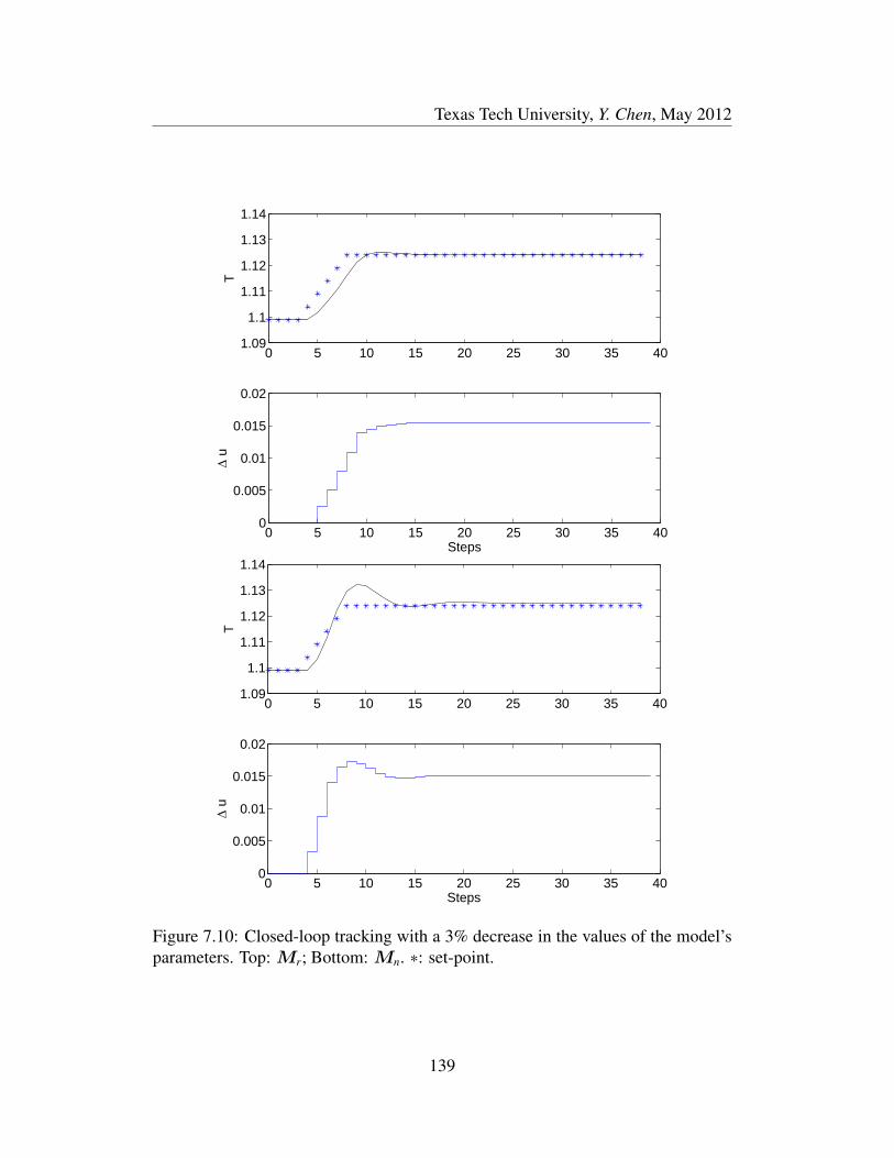
Texas Tech University, Y. Chen, May 2012
0 5 10 15 20 25 30 35 401.09
1.1
1.11
1.12
1.13
1.14T
0 5 10 15 20 25 30 35 400
0.005
0.01
0.015
0.02
Steps
Δ u
0 5 10 15 20 25 30 35 401.09
1.1
1.11
1.12
1.13
1.14
T
0 5 10 15 20 25 30 35 400
0.005
0.01
0.015
0.02
Steps
Δ u
Figure 7.10: Closed-loop tracking with a 3% decrease in the values of the model’sparameters. Top: Mr; Bottom: Mn. ∗: set-point.
139
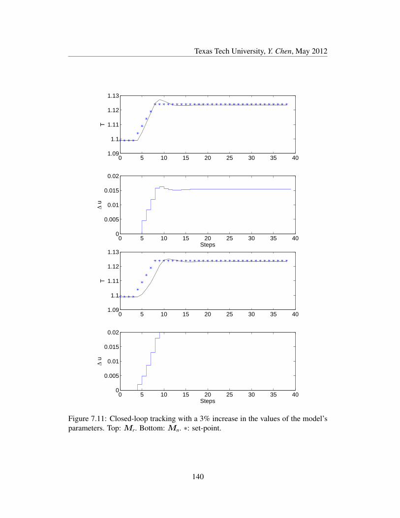
Texas Tech University, Y. Chen, May 2012
0 5 10 15 20 25 30 35 401.09
1.1
1.11
1.12
1.13T
0 5 10 15 20 25 30 35 400
0.005
0.01
0.015
0.02
Steps
Δ u
0 5 10 15 20 25 30 35 401.09
1.1
1.11
1.12
1.13
T
0 5 10 15 20 25 30 35 400
0.005
0.01
0.015
0.02
Steps
Δ u
Figure 7.11: Closed-loop tracking with a 3% increase in the values of the model’sparameters. Top: Mr. Bottom: Mn. ∗: set-point.
140

Texas Tech University, Y. Chen, May 2012
Nomenclature
DLTI discrete linear time-invariant
ITAE integral of time and absolute error
LHHS Latin hypercube Hammersley sampling
MLM maximum likelihood model
MPC model predictive control
PLS partial least squares
C concentration M maximum likelihood modelMN nominal first-principles model Mn DLTI model identified fromMN
T temperatured disturbances d estimates of disturbancese errors u manipulated variablesy model outputs y∗ set-point
yM plant measurement yp plant outputs without disturbancesyPLS outputs from PLS model σ standard deviationΘ uncertain parameters U uniform distribution
Nlog log-normal distribution N normal distribution
141

Texas Tech University, Y. Chen, May 2012
Chapter 8
Summary, Contribution and Future Work
8.1 Summary
A process model in the form of a system of equations can be used to predict
the states of a process in real-time applications such as monitoring, control, fault
detection, scheduling, supply chain management, and so forth. The uncertainty in a
model’s parameters will affect the accuracy of the predictions. Thus, it is justifiable
to study model parameter uncertainty, the subject of this work.
It is desirable to analyze the effects of multiple sensitive parameter uncertainties
on the solutions of a computational model. The distributions of the model’s outputs
can be calculated based on the distributions of the input parameter uncertainties.
There are certain processes, especially large complex systems, where information
about the critical parameters are not known even in a gross manner. In such cases,
initial guesses of these parameters must be updated if the model’s outputs are to be
used for making decisions about the operation of the process. Related to this issue
is the case where some information is known about the parameter values so that
a potential robust estimate can be derived. A model with robust estimates of the
uncertain parameters can provide accurate predictions.
The objectives of this dissertation were to address these issues. Specifically, (i)
142
Texas Tech University, Y. Chen, May 2012
analyze the effect of multiple model uncertain parameters on the model’s outputs,
(ii) update the uncertain parameter values efficiently to improve the prediction ac-
curacy for real-time applications, and (iii) develop a model parameterized by max-
imum likelihood estimates of the parameters to improve the model’s performance.
Following an approach of sampling of the distributions and propagation of the
samples within the model the Latin hypercube Hammersley sampling (LHHS) tech-
nique was applied. By permuting the Latin hypercube samples according to the or-
der of Hammersley points’ sequence, LHHS provided efficient and effective propa-
gation results for multiple dimension uncertain parameters.
To represent the relationships between parameter uncertainties and the model
outputs, partial least squares (PLS) regression was applied. The solution space of a
distributed model of a process is usually of a large dimension. To focus the infor-
mation on the independent directions of variability, a reduced-order model (ROM)
was identified using a Karhunen-Loeve (KL) expansion. This technique has been
shown to concentrate the independent directions of variability in a smaller dimen-
sion whose basis set is made up of empirical eigenfunctions. Thus, the response
variables in the PLS regression were not the large dimension of the solution space
associated with the distributed model but rather the smaller dimension of coeffi-
cients of the empirical eigenfunctions identified by the KL expansion. The use of
the KL expansion to identify the coefficients of the empirical eigenfunctions so that
they can be used as the response variables in the creation of the PLS model is one
143

Texas Tech University, Y. Chen, May 2012
of the contributions of this work.
Updating the uncertain parameter values is necessary to improve the model’s ac-
curacy. In this work, two updating methods, Markov chain Monte Carlo (MCMC)
and an ensemble Kalman filter (EnKF), were designed as a function of the problem
space and compared. The updating methods then were embedded in an optimal con-
trol framework in which the system to be optimally managed was an oil producing
reservoir. It was found that the EnKF method can provide better parameter updat-
ing performance when compared to the MCMC when there are multiple uncertain
parameters to be updated.
Updating is a time consuming process, which is a critical limitation for some
real-time processes. Once there is some information about the uncertain parameter,
such as its sampled values, it is attractive to estimate a likely value with some con-
fidence. This work developed the concept of a maximum likelihood model as that
model which is parameterized with robust estimates of the uncertain parameters.
This work developed the necessary theoretical underpinnings to prove the existence
of this model. Since real process have finite and feasible ranges of the variables,
these ranges are imposed when determining the robust estimates of the uncertain
parameters using both LHHS and the theory of robust statistics. The use of the
maximum likelihood model was demonstrated in an application of state estimation
and model predictive control.
144
Texas Tech University, Y. Chen, May 2012
8.2 Contributions
The contributions of this work are as follows.
1. Use of the Karhunen-Loeve expansion to identify the coefficients of the em-
pirical eigenfunctions so that they can be used as the response variables in the
creation of a partial least squares regression model.
2. It is demonstrated that the maximum likelihood estimate can provide more
accurate estimates of the model uncertain parameters than any other kind of
estimates (e.g., mean, linear estimate, and/or rank estimate).
3. Theoretical underpinnings are developed to establish the existence of a maxi-
mum likelihood model. A maximum likelihood model is parameterized with
robust estimates of the uncertain parameters, found using robust statistics,
that are within the uncertain parameters’ feasible ranges.
8.3 Future Work
This work analyzed model parameter uncertainty for model-based applications.
Many issues remain; below are some suggestions following aspects.
1. The uncertainty analysis in this work was based on the probability theory.
Since possibility theory is another statistical theory for dealing with certain
types of uncertainty it would be worthwhile to investigate the study of uncer-
tainty with a combination of probability and possibility theories.
145

Texas Tech University, Y. Chen, May 2012
2. Real processes are nonlinear, complex, and of high dimension. In this work
the nonlinearity was approximated by assuming that the operation of the pro-
cess is around the designed operating conditions, thus a linear approximation
is justified from which to study small perturbations. As a consequence of
this approximation, in the model-based control framework, a linear controller
was designed. Future work should be focused on developing some form of a
nonlinear controller to regulate the nonlinear process.
3. Although a nonlinear controller may be more appropriate to regulate a non-
linear process, the issue of closed-loop stability cannot be overlooked. Estab-
lishing general closed-loop stability criteria is another study that should be
undertaken.
4. Another important issue is to understand fully the area of particle filters (this
includes MCMC and EnKF) for robust state estimation. These methods suf-
fer from degeneracy and re-sampling. A study that investigates these issues
with the goal of developing the maximum likelihood model for robust state
estimation is intriguing.
5. As stated at the outset of this study, the inaccuracy of a mathematical model
of a process is not only due to model parameter uncertainty. A future study
should focus on other sources of model inaccuracy and then combinations of
reasons for the inaccuracies.
146

Texas Tech University, Y. Chen, May 2012
Nomenclature
EnKF ensemble Kalman filter
KL Karhunen-Loeve
LHHS Latin hypercube Hammersley sampling
MCMC Markov chain Monte Carlo
PLS partial least squares
147

Texas Tech University, Y. Chen, May 2012
Bibliography
[1] Y. Zhang. PLS. Website, http://www.mathworks.com/matlabcentral/fileexchange/16465-pls, 2007. MatLab Central, perform PLS calculation byusing NIPALS algorithm.
[2] D. Zheng and K. A. Hoo. System identification and model-based fordistributed parameter systems. Computers and Chemical Engineering,28:1361–1375, 2004.
[3] G. Nævdal, L. M. Johnsen, S. I. Aanonsen, and E. H. Vefring. Reservoirmonitoring and continuous model updating using ensemble Kalman filter.In Annual Technical Conference and Exhibition. Society of Petoleum Engi-neers, 2003. Denver, Colorado, U.S.A., SPE 84372.
[4] D. Zheng and K.A. Hoo. Low-order model identification for implementablecontrol solutions of distributed parameter systems. Computers and ChemicalEngineering, 26:1049–1076, 2002.
[5] Y. Chen and K.A. Hoo. The development of maximum likelihood model formodel-based applications. Submitted to Computers & Chemical Engineer-ing, 2011.
[6] C. E. Garcia and M. Morari. Internal model control. 1. A unifying reviewand some new results. Industrial & Engineering Chemistry Process Designand Development, 21:308–303, 1982.
[7] D. Zheng. System identification and model-based control for a class of dis-tributed parameter systems. Doctor of philosophy, Texas Tech University,Lubbock, TX, 2002.
[8] P. M. Verderame and C. A. Floudas. Operational planning for large-scaleindustrial batch plants under demand due date and amount uncertainty: II.Conditional value-at-risk framework. Industrial and Engineering ChemistryReasearch, 49:260–275, 2010.
[9] P. M. Verderame and C. A. Floudas. Integration of operational planningand medium-term scheduling for large-scale industrial batch plants underdemand and processing time uncertainty. Industrial and Engineering Chem-istry Reasearch, 49:4948–4965, 2010.
[10] P. M. Verderame, J. A. Elia, J. Li, and C. A. Floudas. Planning and schedul-ing under uncertainty: A review across multiple sectors. Industrial and En-gineering Chemistry Reasearch, 49:3993–4017, 2010.
[11] D. Xiu and G.E. Karniadakis. Modeling uncertainty in flow simulationsvia generalized polynomial chaos. J. Computational Physics, 187:137–167,2003.
148

Texas Tech University, Y. Chen, May 2012
[12] M. A. Tatang, W. Pan, R. G. Prinn, and G. J. McRae. An efficient method forparametric uncertainty analysis of numerical geophysical models. Journal ofgeophysical research, 102:21925–21932, 1997.
[13] M. Pertile and M. D. Cecco. Uncrtainty evaluation for complex propaga-tion models by means of the theory of evidence. Measurement science andtechnology, 19:1–10, 2008.
[14] R. Wang, U. Diwekar, and C. E. Gregoire Padro. Efficient sampling tech-niques for uncertainties in risk analysis. Environmental Progress, 23:141–157, 2004.
[15] T. Wong, W. Luk, and P. Heng. Sampling with hammersley and halton points.Journal of Graphics Tools, 2:9–24, 1997.
[16] J. R. Kalagnanam and U. M. Diwekar. An efficient sampling technique foroff-line quality control. Technometrics, 39(3):308–319, 1997.
[17] K. Subranmanyan, Y. Wu, U. M. Diwekar, and M. Q. Wang. New stochasticsimulation capacity applied to the greet model. International journal of lifecycle assessment, 13(3):278–285, 2008.
[18] Y. Chen and K.A. Hoo. Uncertainty propagation for effective reduced-ordermodel generation. Computers and Chemical Engineering, 34:1597–1605,2010.
[19] Y. Chen and K.A. Hoo. Uncertainty propagation for efficient model-basedcontrol solutions. In Proceedings of the 2010American Control Conference,pages 3112–3117, Baltimore, Maryland, June & July 2010. ThA22.1.
[20] S. M. Stigler. Thomas Bayes’ Bayesian inference. Journal of the RoyalStatistical Society, 145:250–258, 1982.
[21] T. J. Ulrych, M. D. Sacchi, and A. G. Woodbury. A bayes tour of inversion:A tutorial. Geophysics, 66:55–69, 2001.
[22] P. J. Green. Reversible jump Markov chain Monte Carlo computation andBayesian model determination. Biometrika, 82:711–732, 1995.
[23] H. Haario, E. Saksman, and J. Tamminen. An adaptive metropolis algorithm.Bernoulli, 7:223–242, 2001.
[24] C. Andrieu, N. D. Freitas, A. Doucet, and M. I. Jordan. An introduction toMCMC for machine learning. Machine Learning, 50:5–43, 2003.
[25] G. Evensen. Sequential data assimilation with nonlinear quasi-geostrophicmodel using monte carlo methods to forecast error statistics. Journal of Geo-physical Research, 99:143–162, 1994.
149

Texas Tech University, Y. Chen, May 2012
[26] G. Burgers, P. J. van Leeuwen, and G. Evensen. Analysis scheme in theensemble Kalman filter. Monthly Weather Review, 126:1719–1724, 1998.
[27] G. Evensen. The ensemble Kalman filter: Theoretical formulation and prac-tical implementation. Ocean Dynamics, 53:343–367, 2003.
[28] G. Evensen. Sampling strategies and square root analysis schemes for theEnKF. Ocean Dynamics, 54:539–560, 2004.
[29] G. Evensen. Data assimilation : The ensemble Kalman filter. Springer,Berlin, 2007.
[30] L. Marshall, D. Nott, and A. Sharma. A comparative study of Markovchain Mote Carlo methods for conceptual rainfall-runoff modeling. WaterResources Research, 40, 2004. W02501, doi:10.1029/2003WR002378.
[31] B. C. Bates and E. P. Campbell. A Markov chain Monte Carlo scheme forparameter estimation and inference in conceptual rainfall-runoff modeling.Water Resource Research, 37:937–947, 2001.
[32] A. E Hassan, H. M. Bekhit, and J. B. Chapman. Using Markov chain MonteCarlo to quantify parameter uncertainty and its effect on predictions of agroundwater flow model. Environmental Modelling & Software, 24:749–763, 2009.
[33] P. L. Houtekamer and L. M Herschel. Data assimilation using an ensembleKalman filter technique. Monthly Weather Review, 126:796–811, 1998.
[34] A. W. Heemink, M. Verlaan, and A. J. Segers. Variance reduced ensembleKalman filtering. Monthly Weather Review, 129:1718–1728, 2001.
[35] G. Nævdal, T. Mannseth, and E. H. Vefring. Near-well reservoir monitor-ing through ensemble Kalman filter. In Improved Oil Recovery Symposium.Society of Petoleum Engineers, 2002. Tulsa, Oklahoma, U.S.A., SPE 75235.
[36] Y. Gu and D. S. Olive. History matching of the PUNQ-S3 reservoir modelusing ensemble Kalman filter. In Annual Technical Conference and Exhi-bition. Society of Petoleum Engineers, 2004. Houston, Texas, U.S.A., SPE89942.
[37] J. P. Jensen. Ensemble Kalman filtering for state and parameter estimation ona reservoir model. Master of science in engineering cybernetics, NorweigianUniversity of Science and Technology, June 2007.
[38] Y. Chen and K.A. Hoo. Model parameter uncertainty updates to achieve opti-mal management of a reservoir. Submitted to Control Engineering Practice,2011.
[39] P. J. Huber. Robust Statistics. John Wiley & Sons, Inc, 1981.
150

Texas Tech University, Y. Chen, May 2012
[40] P. J. Rousseeuw and A. M Leroy. Robust Regression and Outlier Detection.John Wiley and Sons, New York, 1987.
[41] R. G. Staudte and S. J. Sheather. Robust Estimation and Testing. John Wileyand Sons, New York, 1990.
[42] D.J. Olive. Applied Robust Statistics. 2008.
[43] M. Daszykowski, K. Kaczmarek, Y. Vander Heyden, and B. Walczak. Ro-bust statistics in data analysis–a review:: Basic concepts. Chemometrics andintelligent laboratory systems, 85(2):203–219, 2007.
[44] C. E. Garcia and A. M. Morshedi. Quadratic programming solution of dy-namic control (QDMC). Chemical Engineering Communications, 46:73–87,1986.
[45] C.R. Cutler and BL Ramaker. Dynamic matrix control-a computer controlalgorithm. In Proceedings of the joint automatic control conference, pages13–15, 1980.
[46] C.R. Cutler. Dynamic matrix control: An optimal multivariable control algo-rithm with constraints. Dissertation Abstracts International Part B: Scienceand Engineering, 44(8), 1984.
[47] P. L. Lee and G. R. Sullivan. Generic model control (GMC). Computers &chemical engineering, 12(6):573–580, 1988.
[48] D. W. Clarke, C. Mohtadi, and P. S. Tuffs. Generalized predictive control–Part I. the basic algorithm. Automatica, 23(2):137–148, 1987.
[49] D. Zheng and K.A. Hoo. Low-order control-relevant models for a class ofdistributed parameter systems. Chemical Engineering Science, 56:6683–6710, 2001.
[50] D. Zheng and K.A. Hoo. Low-order model identification of distributedparameter systems by a combination of singular value decompositionand karhunen-loeve expansion. Industrial and Engineering ChemistryReasearch, 41:1545–1556, 2002.
[51] P. Astrid. Reduction of process simulation models a proper orthogonal de-composition approach. Doctor of philosophy, Eindhoven University of Tech-nology, Netherlands, 2004.
[52] Y. Lang, A. Malacina, L. T. Bieger, S. Munteanu, J. I. Madsen, and S. E.Zitney. Reduced order model based on principal component analysis forprocess simulation and optimization. Energy & Fuels, 23:1695–1706, 2009.
151

Texas Tech University, Y. Chen, May 2012
[53] J. F. MacGregor, H. Yu, S. G. Munoz, and J. Flores-Cerrillo. Data-basedlatent variable methods for process analysis, monitoring and control. Com-puters and Chemical Engineering, 29:1217–1223, 2005.
[54] N. Townsend. Implementation of control policies for ARMAX models. UlamQuarterly, 2:57–64, 1994.
[55] B. D. Ripley. Stochastic Simulation. Wiley & Sons, 1987.
[56] S. S. Sawilowsky. You think you’ve got trivials? Journal of Modern AppliedStatistical Methods, 2:218–225, 2003.
[57] E. C. Anderson. Monte carlo methods and importance sampling. Technicalreport, 1999.
[58] G. D. Wyss and K. H. Jorgensen. A user’s guide to LHS: Sandia’s Latinhypercube sampling software. Technical Report Technical Report SAND98-0210, Sandia National Laboratories, Albuquerque, NM, 1998.
[59] E. Rafajłowicz and R. Schwabe. Halton and Hammersley sequences in mul-tivariate nonparametric regression. Statistics & Probability Letters, 76:803–812, 2006.
[60] R. L. Iman and W. J. Conover. A distribution-free apprach to inducing rankcorrelation among input variables. Communications on Statistics: Simulationand Computing, 11(3):311–334, 1982.
[61] J. M. Douglas. Conceptal design of chemical processes. NY: McGraw-Hill,New York, 1988.
[62] H. Abdi. Partial Least Squares (PLS) Regression, pages 792–795. Sage,Thousand Oaks (CA), 2003.
[63] L. Sirovich. New Perspectives in Turbulence. Springer-Verlag, New York,NY, 1st edition, 1991.
[64] A. J. Newman. Model reduction via the karhunen-loeve expansion Part I: anexposition technical report t.r. 96-32. Technical report, University of Mary-land, College Park,MD, 1996.
[65] L. Sirovich, B. W. Knight, and J. D. Rodriguez. Optimal low-dimensionaldynamical approximations. Quarterly of applied mathematics, 48:535–548,1990.
[66] Y. Chen and K.A. Hoo. Optimal model-based reservoir management withmodel parameter uncertainty updates. In The 4th International Symposiumon Advanced Control of Industrial Processes, Hangzhou, China, May 2011.
152

Texas Tech University, Y. Chen, May 2012
[67] A. G. Gelman and W. R. Gilks. Efficient Metropolis jumping rules. BayesianStatistics, 5:599–607, 1996.
[68] R. M. May. Simple mathematical models with very complicated dynamics.Nature, 261(5560):459–467, 1976.
[69] M. Latil. Enhanced Oil Recovery. Gulf Publishing Co, Paris, French, edi-tions technip edition, 1980.
[70] T. L. Giles. Effects of permeability on waterflooding efficiency. Technicalreport, Texas Tech University, 2008.
[71] P. Sarma, L.J. Durlofsky, K. Aziz, and W.H. Chen. Efficient real-time reser-voir management using adjoint-based optimal control and model updating.Computational Geosciences, 10:3–36, 2006.
[72] E. Suwartadi, S. Krogstad, and B. Foss. Nonlinear output constraints han-dling for production optimization of oil reservoirs. Computational Geo-sciences, pages 1–19, 2011.
[73] N. El-Khatib. Waterflooding performance of communicating stratified reser-voirs with log-normal permeability distribution. In Middle East Oil Showand Conference, 1997.
[74] P. Sarma, L. J. Durlofsky, and K. Aziz. Efficient closed-loop productionoptimization under uncertainty. In Proc. 14th European Biennial Conference.Society of Petoleum Engineers, 2005. Madrid, Spain, SPE 94241.
[75] V.L. Bageshwar and F. Borrelli. Observer pole placement limitations for aclass of offset-free model predictive controllers. In Proceedings of the 2011American Control Conference, Seattle, Washington, June 2008.
[76] R. Gondhalekar and C.N. Jones. Mpc of constrained discrete-time linearperiodic systems–a framework for asynchronous control: Strong feasibility,stability and optimality via periodic invariance. Automatica, 47, 2010.
[77] B. A. Ogunnaike and W. H. Ray. Process dynamics, modeling, and control.NY:Oxford, New York, 1994.
[78] H. Kwakernaak and R. Sivan. The maximally achievable accuracy of lin-ear optimal regulators and linear optimal filters. Automatic Control, IEEETransactions on, 17(1):79–86, 1972.
[79] M. Athans. The role and use of the stochastic linear-quadratic-gaussian prob-lem in control system design. Automatic Control, IEEE Transactions on,16(6):529–552, 1971.
153
Texas Tech University, Y. Chen, May 2012
[80] B. Minasny and P. J. Acklam. Latin Hypercube Sampling. Web-site, http://www.mathworks.com/matlabcentral/fileexchange/4352-latin-hypercube-sampling/content/ltqnorm.m, 2004. MatLab Central, LatinHypercube Sampling.
[81] I. Aitokhehi and L.J. Durlofsky. Optimizing the performance of smart wellsin complex reservoirs using continuously updated geological models. J.Petroleum Science & Engineering, 48:254–264, 2005.
[82] N.R. Amundson. Mathemtical Methods in Chemical Engineering. Prentice-Hall, New York, NY, 1966.
[83] J. E. Arbogast and J. Cooper, D. Extension of IMC tuning correlation fornon-self requlating (integrating) processes. ISA Transactions, 46:303–311,2007.
[84] R.B. Ash and M.F. Gardner. Topics in Stochastic Processes. Academic Press,New York, NY, 1975.
[85] K. J. Åstrom and T. Hagglund. PID Controllers: Theory, Design and Tuning.Instrument Society of America, Research Triangle Park, NC, 1995.
[86] K. J. Åstrom, H. Panagopoulos, and T. Hagglund. Design of PI controllersbased on non-convex optimization. Automatica, 34:585–601, 1998.
[87] K. J. Åstrom and T. Hagglund. Revisiting the Ziegler–Nichols step responsemethod for PID control. Journal of Process Control, 14:635–650, 2004.
[88] K. J. Beers. Numerical methods for chemical engineering applications inMatLab R©. Oxford University Press, New York, NY, 2007.
[89] A. Benabdallah and M. A. Hammami. Circle and Popov criterion for outputfeed back stabilization of uncertain systems. Nonlinear Analysis: Modelingand Control, 11:137–148, 2006.
[90] D. R. Brouwer and J. D. Jansen. Dynamic optimization of water floodingwith smart wells using optimal control theory. In Proc. 13th EuropeanPetroleum Conference. Society of Petoleum Engineers, 2002. Aberdeen,Scotland, U.K., SPE 78278.
[91] D. R. Brouwer, J. D. Nævdal, G. Jansen, E. H. Vefring, and C. P. J. W. vanKruijsdijk. Improved reservoir management through optimal control andcontinuous model updating. In Annual Technical Conference and Exhinition.Society of Petoleum Engineers, 2004. Houston, Texas, U.S.A., SPE 90149.
[92] D. R. Brouwer. Dynamic Water Flood Optimization with Smart Wells usingOptimal Control Theory. Doctor of philosophy, Delft Univ. of Tech., Delft,Netherlands, 2004.
154

Texas Tech University, Y. Chen, May 2012
[93] G. A. Brusher, P. T. Kabamba, and A. G. Ulsoy. Coupling between the mod-eling and controller-design problems - Part I: Analysis. Transactions of theASME, 119:498–502, 1997.
[94] M. Buckley and J. Wall. Microbial energy conversion. Microbial En-ergy Conversion, pages 1–20, 2006. Colloquium sponsored by AmericanAcademy of Microbiology.
[95] A. J. Burnham, J. F. MacGregor, and R. Viveros. A statistical framwworkfor multivariate latent variable regression methods based on maximum like-lihood. Journal of Chemometrics, 13:49–65, 1999.
[96] M. A. Cardoso, L. J. Durlofsky, and P. Sarma. Development and applicationof reduced-order modeling procedures for subsurface flow simulation. Inter-national Journal for Numerical Methods in Engineering, 77(9):1322–1350,2009.
[97] Y. Chen. Comparison of discrete controller designs applied to the requlationof a plug flow reactor. Technical report, Texas Tech University, 2010.
[98] Y. Chen and K.A. Hoo. Temperature regulation of a novel plate reactor withmultiple feed ports. Submitted to Industrial & Engineering Chemistry Re-search, 2011.
[99] Y. Chen and K.A. Hoo. Optimization of reservoirs with model parameteruncertainty updates. In Extended Abstracts 2010 AIChE, Salt Lake City, UT,Nov 2010.
[100] Y. Chen and K.A. Hoo. Application of partial least squares reqression in thestudy of uncertainty. In Proceedings of the 2011 American Control Confer-ence, San Francisco, California, June & July 2011.
[101] S. V. Emets. An examination of modified hierarchical design structure forchemical processes. Master of science, Texas Tech University, May 2003.
[102] L. M. Eriksson and M. Johansson. Simple PID tuning rules for varying time-delay systems. In IEEE Conference on Decision and Control, New Orleans,LA, December 2007.
[103] A. Ferrero and S. Salicone. The random-fuzzy variables: A new approach tothe expression of uncertainty in measurement. In IEEE Transactions on In-strumentation and Measurement, volume 53, pages 1370–1377, 2004. num-ber 5.
[104] A. Ferrero and S. Salicone. A comparative anlaysis of the statistical andrandom-fuzzy approaches in the expression of uncertainty in measurement.In IEEE Transactions on Instrumentation and Measurement, volume 54,pages 1475–1481, 2005. number 4.
155

Texas Tech University, Y. Chen, May 2012
[105] A. Ferrero and S. Salicone. Fully comprehensive mathematical approach tothe expression of uncertainty in measurement. In IEEE Transactions on In-strumentation and Measurement, volume 55, pages 706–712, 2006. number3.
[106] A. Ferrero and S. Salicone. Modeling and preocessing measurement uncer-tainty within the theory of evidence: Mathematics of random-fuzzy vari-ables. In IEEE Transactions on Instrumentation and Measurement, vol-ume 56, pages 704–716, 2007. number 3.
[107] A. Ferrero and S. Salicone. An original fuzzy method for the comparison ofmeasuremnet results represented as random-fuzzy variables. In IEEE Trans-actions on Instrumentation and Measurement, volume 56, pages 1292–1299,2007. number 4.
[108] R. V. Field, Jr., Student member, and ASCE. Numerical methods to estimatethe coefficients of the polynomial chaos expansion. In Proceedings of the15th ASCE engineering mechanics conference, Columbia University, NewYork, June 2002. American Society of Civil Engineers.
[109] J. Flores-Cerrillo and J. F. MacGregor. Control of batch product qualityby trajectory manipulation using latent variable models. Journal of ProcessControl, 14:539–553, 2003.
[110] D. H. Gay and W. H. Ray. Identification and control of distributed parametersystems by means of the singular value decomposition. Chemical Engineer-ing Science, 50:1519–1539, 1995.
[111] A Gelb. Applied Optimal Estimation. The MIT Press, Cambridge, MA,1974.
[112] M.D. Grau, J.M. Nougues, and L. Puigjaner. Batch and semibatch reactorperformance for an exothermic reaction. Chemical Engineering and Pro-cessing, 39:141–148, 2000.
[113] A. C. Grosse, G. W. Dicinoski, M. J. Shaw, and P. R. Haddad. Leachingand recovery of gold using ammoniacal thiosulfate leach liquors (a review).Hydrometallurgy, 69:1–21, 2003.
[114] T. Hagglund and K. J. Åstrom. Revisiting the Ziegler-Nichols tuning rulesfor PI control. Asian Journal of Control, 4:364–380, 2002.
[115] T. Hagglund and K. J. Åstrom. Revisiting the Ziegler-Nichols tuning rulesfor PI control – part II the frequency response method. Asian Journal ofControl, 6:469–482, 2004.
[116] S. Haugwitz. Modeling, Control and Optimization of a Plate Reactor. Doctorof philosophy, Lund Institute of Technology, Lund, Sweden, 2007.
156

Texas Tech University, Y. Chen, May 2012
[117] S. Haugwitz, P. Hagander, and T. Nore. Modeling and control of a novelheat exchange reactor, the open plate reactor. Control Engineering Practice,15:779–792, 2007.
[118] P. Holmes, J.L. Lumley, and G. Berkooz. Turbulence, Coherent Structures,dynamical systems and symmetry. Cambridge University Press, New York,NY, 1996.
[119] K. A. Hoo and D. Zheng. Low-order control-relevant models for a classof distributed parameter systems. Chemical Engineering Science, 56:6683–6710, 2001.
[120] V. Janickis, R. Ivanauskas, R. Stokiene, and N. Kreiveniene. The modifica-tion of polyamide 6 films by thallium sulfide layers using dodecationic acid.Materials Science, 12:311–317, 2006.
[121] J. D. Jansen, D. R. Brouwer, G. Nævdal, and van Kruijsdijk C. P. J. W.Closed-loop reservoir management. First Break, 23:43–48, 2005.
[122] R. E. Kalman and J.E. Bertram. General synthesis procedure for computercontrol of single-loop and multi-loop systems. AIEE Trans, 77, Part 2:602,1958.
[123] R. E. Kalman and J. E. Bertram. A unified approach to the theory of samplingsystems. Journal of The Franklin Institute, 267:405–436, 1959.
[124] H. K Khalil. Nonlinear Systems. NJ: Prentic Hall, 2nd edition, 1996.
[125] P. S. Koutsourelakis. Design of complex systems in the presence of large un-certainties: A statistical approach. Computer Methods in Applied Mechanicsand Engineering, 197:4092–4103, 2008.
[126] J. Lee and T. F. Edgar. Multiloop PI/PID control system improvement via ad-justing the dominant pole or the peak amplitude ratio. Chemical EngineeringScience, 61:1658–1666, 2006.
[127] R. Li, A.C. Reynolds, and D.S. Oliver. History matching of three-phase flowproduction data. In Proceedings of 14th European Biennial Conference. Soc.Pet. Eng., 2005. Houston, TX, SPE 66351.
[128] W. L. Luyben. Simple method for tuning SISO controllers in multivariablesystems. Industrial & Engineering Chemistry Process Design and Develop-ment, 25:654–660, 1986.
[129] U. Mann. Principles of Chemical Reactor Analysis and Design. Plains pub-lishing company, Lubbcok, Texas, 1999.
[130] R. A. Maronna, R. Douglas Martin, and V. J. Yohai. Robust statistics : theoryand methods. J. Wiley, Chichester, England; Hoboken, NJ, 2006.
157

Texas Tech University, Y. Chen, May 2012
[131] P. Meum. Optimal reservoir control using nonlinear MPC and ECLIPSE.Master of science in engineering cybernetics, Norweigian University of Sci-ence and Technology, June 2007.
[132] P. Meum, P. Tøndel, J-M. Godhavn, and O. M. Aamo. Optimization of smartwell production through nonlinear model predictive control. In IntelligentEnergy Conference and Exhibition. Society of Petoleum Engineers, 2008.Amsterdam, Netherlands, SPE 112100.
[133] G. Nævdal, D. R. Brouwer, and J-D. Jansen. Waterflooding using closed-loop control. Computational Geosciences, 10:37–60, 2006.
[134] A. J. Newman. Model reduction via the karhunen-loeve expansion Part II:some elementary technical report t.r. 96-33. Technical report, University ofMaryland, College Park,MD, 1996.
[135] D. E. Rivera, M. Morari, and S. Skogestad. Internal model control. 4. PIDcontroler design. Industrial and Engineering Chemistry Process Design andDevelopment, 25:252–265, 1986.
[136] S. Salicone. Measurement Uncertainty: An Approach via the MathematicalTheory of Evidence. Springer, Berlin, Ger, 2007.
[137] P. Sarma, K. Aziz, and L. J. Durlofsky. Implementation of adjoint solutionfor optimal control of smart wells. In Proc. Reservoir Symposium. Soc. Pet.Eng., 2005. Houston, TX, SPE 92864.
[138] V. S. Shabde, K. A. Hoo, and Zheng D. Accelerated karhunen-loeve expan-sion: A nonlinear model reduction. In DYCOPS-7, Boston, MA, July 2004.
[139] D. E. Seborg, T. F. Edgar, and D. A. Mechllichamp. Process Dynamics andContol. Wiley, New York, 2nd edition, 2004.
[140] S. K. Singh. Computer-Aided Process Control. Prentice-Hall of India, 2004.
[141] S. Tavakoli, I. Griffin, and P. J. Fleming. Tuning of decentralised PI (PID)controllers for TITO processes. Control Engineering Practice, 14:1069–1080, 2006.
[142] J. F. M. van Doren, R. Markovinovic, and J-D. Jansen. Reduced-order opti-mal control of water flooding using proper orthogonal decomposition. Com-putational Geosciences, 10:137–158, 2006.
[143] P. M. Verderame and C. A. Floudas. Integrated operational planning andmidium-term scheduling for large-scale industrial batch plants. Industrialand Engineering Chemistry Reasearch, 47:4845–4860, 2008.
158
Texas Tech University, Y. Chen, May 2012
[144] P. M. Verderame and C. A. Floudas. Operational planning framwork formultisite production and distribution networks. Computers and ChemicalEngineering, 33:1036–1050, 2009.
[145] P. M. Verderame and C. A. Floudas. Operational planning for large-scaleindustrial batch plants under demand due date and amount uncertainty: I.Robust optimization framework. Industrial and Engineering ChemistryReasearch, 48:7214–7231, 2009.
[146] T. N. L. Vu, J. Lee, and M. Lee. Design of multi-loop PID controllers basedon the generalized IMC-PID method with Mp criterion. International Jour-nal of Control, Automation, and System, 5:212–217, 2007.
[147] Y. You. Approximate inertial manifolds for nonlinear parabolic equations viasteady-state determining mapping. Intl. J. Math. & Math. Sci., 18(1):1–24,1995.
[148] H. Yu, C. Y. Chung, K. P. Yong, H. W. Lee, and J. H. Zhang. Probabilis-tic load flow evaluation with hybrid latin hypercube-sampling and choleskydecomposition. In IEEE Transactions On Power System, volume 24, pages667–667, 2009. number 2.
[149] L. A. Zadeh. Fuzzy sets as a basis for a theory of possibility. Fuzzy Sets andSystems, 1:3–28, 1978.
[150] H. Zhang and D. B. Dreisinger. The recovery of gold from ammoniacalthiosulfate solutions containing copper using ion exchange resin columns.Hydrometallurgy, 70:225–234, 2004.
[151] J. G. Ziegler, N. B. Nichols, and N. Y. Rochester. Optimum setting for auto-matic controllers. Trans. ASME, 64:759–768, 1942.
159

Texas Tech University, Y. Chen, May 2012
Appendix A
Preliminaries on Model-based Control
The regulation of the dynamic behavior of the process to some desired target is
the goal of the control system. This goal must be achieved within the constraints
of the process and any other limits imposed by the environment, health and safety
policies. Model-based control is concerned with the explicit use of a model of
the process to determine the control inputs to regulate the process. Model-based
control has roots in optimal control theory and linear and nonlinear system theory.
The simplest optimal controller is the linear quadratic regulator (LQR) [78] or a
state-feedback controller. In contrast, the solution to the control of uncertain linear
systems disturbed by additive white Gaussian noise is the linear quadratic Gaussian
(LQG) controller [79].
There are multiple the model-based control frameworks but they can be classi-
fied in two distinct categories. First is the direct synthesis approach. A trajectory is
specified for the desired plant output behavior. The process model is used directly
to synthesize the controller required to cause the process output to follow the tra-
jectory exactly. The most common approach is what is known as internal model
control [77].
Figure A.1 illustrates an internal model control framework. In this figure, a
process model which describes the process behavior is used. The controller outputs
u are input to both the process and the model. The difference between the plant
measurements ym and model outputs y is an estimation of disturbances (d) and any
process/model mismatch. Given a desired set-point trajectory, y∗, the controller
160

Texas Tech University, Y. Chen, May 2012
outputs are calculated based on the difference between the process measurements
and the model outputs.
du ym+
+
+-
y* Controller Plant
Modely
-
+
Figure A.1: Internal model control framework [6]. y∗: desired set-points trajectory,u: controller outputs, ym: process measurements, y: model outputs, d: measuredor unmeasured disturbances.
Second is the optimization approach. An objective function such as Equation
(A.1) is formulated for the desired output behavior. The model is used to derive
the controller required to minimize (or maximize) the objective function. In the
optimization objective, operating constraints are almost always included.
J = (y∗ − y)TQ(y∗ − y) + ∆uTR∆u
sub ject to :
y = M (x,u,Θ)
y ∈ [ymin,ymax]
x ∈ [xmin,xmax]
u ∈ [umin,umax]
∆u ∈ [∆umin,∆umax]
(A.1)
where x ∈ RM are the state variables which are in the constraint [xmin,xmax]; y ∈
RN are controlled variables which are in the constrain [ymin,ymax]; y∗ are the set-
points of y; u ∈ RL are controller outputs which are in the constrain [umin,umax];
∆u are the changes of the input variables between the previous and current control
161
Texas Tech University, Y. Chen, May 2012
step and are in the constrain [∆umin,∆umax]; M is the process model. Q is the
weighting coefficient matrix reflecting the relative importance of y and R is the
weighting coefficient matrix penalizing relative big changes in u.
Model Predictive Control
Since this work is concerned with a form of model-based control, model pre-
dictive control (MPC), the overview that follows is focused on MPC.
Figure A.2 illustrates the basic principle of model predictive control.
k k+1 k+2 k+pk+mk-1k-2k-3
umin
umax
Control Horizon, m
Input Variable
Past MovesPlanned Moves
ymax
Set-point
ymin
Prediction Horizon, p
Controlled Variable MeasurementsEstimations
Figure A.2: A MPC scheme [7]. y: controlled variable; u: controller output.
With the current process measurements at step k, the control inputs of the system
162

Texas Tech University, Y. Chen, May 2012
from step k to a control horizon, M, that is, k, . . . , k+M are determined and based
on these inputs the dynamic behavior of the system from step k to a prediction
horizon P (k, . . . , k + P) is predicted by minimizing an objective function (A.2).
Only the optimal control inputs determined for step k are implemented. At the next
step, k+1, new measurements are obtained and the objective function is resolved to
generate the optimal control inputs that would cause the outputs to meet the desired
behavior k + 1, . . . , k + 1 + P steps into the future.
J =∑P
k=0(y∗ − y)TQ(y∗ − y) +∑M
k=0 ∆uTR∆u
sub ject to :
yk+1 = M (xk,uk,Θ)
y ∈ [ymin,ymax]
x ∈ [xmin,xmax]
u ∈ [umin,umax]
∆u ∈ [∆umin,∆umax]
(A.2)
where the symbols in this equation has the same meaning as Equation A.1. ∆uk =
uk − uk−1. M and P are the control and prediction horizons, respectively. The
difference between this MPC objective function and previous model-based control
objective function (A.1) is Equation (A.2) optimizes the controller outputs over
the control horizon; while Equation (A.1) only is concerned with estimation of the
controller outputs at the current step without regard to future behavior.
163

Texas Tech University, Y. Chen, May 2012
Nomenclature
IMC internal model control
LQG linear quadratic Gaussian
LQR linear quadratic regulator
MPC model predictive control
M process model T transposed disturbance k control stepm control horizon p prediction horizonu controller outputs y process model outputsym plant measurements y∗ set-pointsΘ model parameters
164

Texas Tech University, Y. Chen, May 2012
Appendix B
Computer Programs
In this appendix, the programs for the following algorithms and models are
listed.
1. Hammersley points generation
2. Karhunen-Loeve (KL) expansion
3. Partial least squares regression
4. Markov chain Monte Carlo
5. Generation of Monte Carlo samples
6. Ensemble Kalman filter
7. Robust statistics
8. Model predictive control
9. HDA Process
10. Tubular reactor
B.1 Hammersley Points Generation
function POINT = HHSmatrix(N, k)
% Inputs:
% N: the number of samples for each dimension;
165
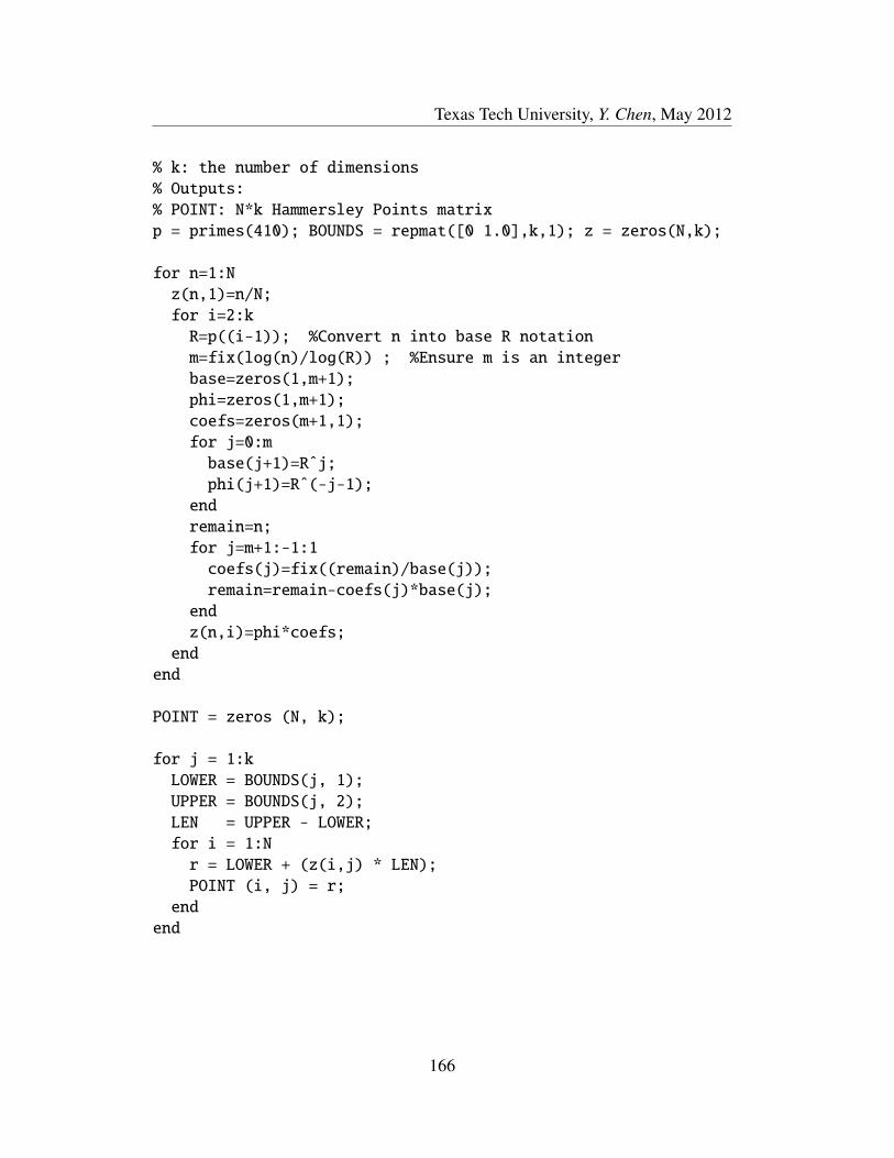
Texas Tech University, Y. Chen, May 2012
% k: the number of dimensions
% Outputs:
% POINT: N*k Hammersley Points matrix
p = primes(410); BOUNDS = repmat([0 1.0],k,1); z = zeros(N,k);
for n=1:N
z(n,1)=n/N;
for i=2:k
R=p((i-1)); %Convert n into base R notation
m=fix(log(n)/log(R)) ; %Ensure m is an integer
base=zeros(1,m+1);
phi=zeros(1,m+1);
coefs=zeros(m+1,1);
for j=0:m
base(j+1)=Rˆj;
phi(j+1)=Rˆ(-j-1);
end
remain=n;
for j=m+1:-1:1
coefs(j)=fix((remain)/base(j));
remain=remain-coefs(j)*base(j);
end
z(n,i)=phi*coefs;
end
end
POINT = zeros (N, k);
for j = 1:k
LOWER = BOUNDS(j, 1);
UPPER = BOUNDS(j, 2);
LEN = UPPER - LOWER;
for i = 1:N
r = LOWER + (z(i,j) * LEN);
POINT (i, j) = r;
end
end
166
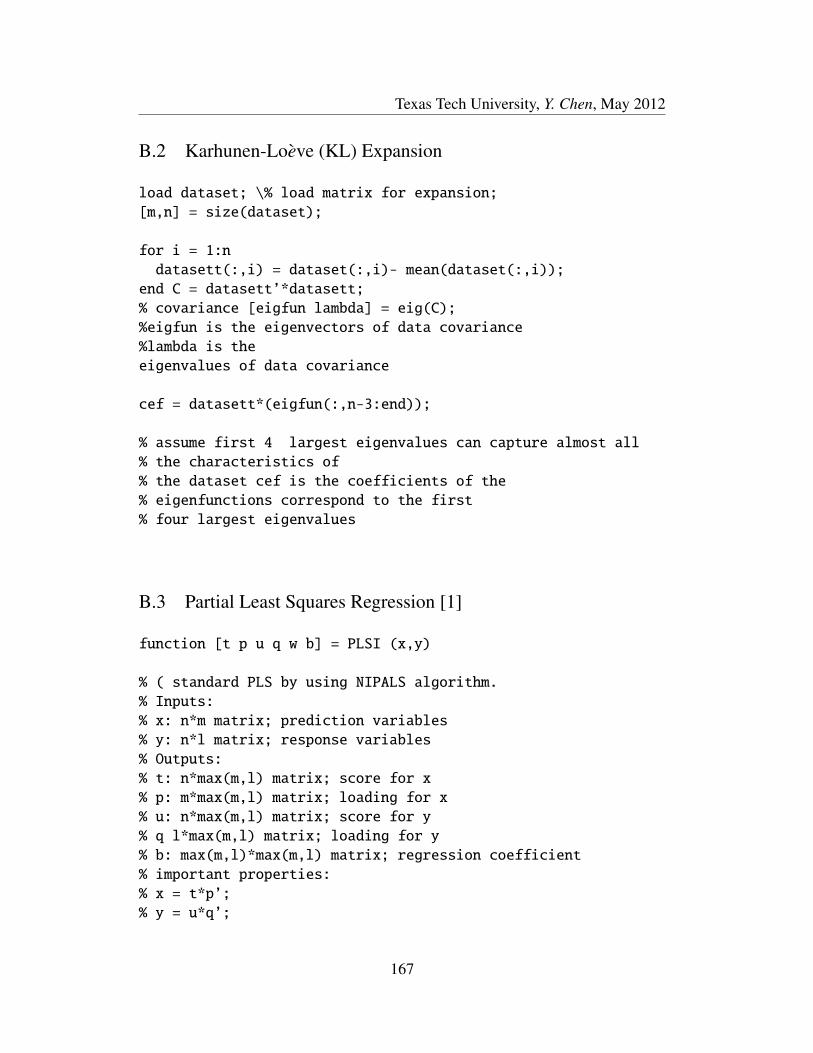
Texas Tech University, Y. Chen, May 2012
B.2 Karhunen-Loeve (KL) Expansion
load dataset; \% load matrix for expansion;
[m,n] = size(dataset);
for i = 1:n
datasett(:,i) = dataset(:,i)- mean(dataset(:,i));
end C = datasett’*datasett;
% covariance [eigfun lambda] = eig(C);
%eigfun is the eigenvectors of data covariance
%lambda is the
eigenvalues of data covariance
cef = datasett*(eigfun(:,n-3:end));
% assume first 4 largest eigenvalues can capture almost all
% the characteristics of
% the dataset cef is the coefficients of the
% eigenfunctions correspond to the first
% four largest eigenvalues
B.3 Partial Least Squares Regression [1]
function [t p u q w b] = PLSI (x,y)
% ( standard PLS by using NIPALS algorithm.
% Inputs:
% x: n*m matrix; prediction variables
% y: n*l matrix; response variables
% Outputs:
% t: n*max(m,l) matrix; score for x
% p: m*max(m,l) matrix; loading for x
% u: n*max(m,l) matrix; score for y
% q l*max(m,l) matrix; loading for y
% b: max(m,l)*max(m,l) matrix; regression coefficient
% important properties:
% x = t*p’;
% y = u*q’;
167
Texas Tech University, Y. Chen, May 2012
% ti’ * tj = 0;
% wi’ * wj = 0; )
[nX,mX] = size(x);
[nY,mY] = size(y);
nMaxIteration = max([mX,mY]);
nMaxOuter = 10000;
for iIteration = 1:nMaxIteration
% choose the column of x has the largest square of sum as t.
% choose the column of y has the largest square of sum as u.
[dummy,tNum] = max(diag(x’*x));
[dummy,uNum] = max(diag(y’*y));
tTemp = x(:,tNum);
uTemp = y(:,uNum);
% iteration for outer modeling
for iOuter = 1 : nMaxOuter
wTemp = x’ * uTemp/ norm(x’ * uTemp);
tNew = x * wTemp;
qTemp = y’ * tNew/ norm (y’ * tNew);
uTemp = y * qTemp;
if norm(tTemp - tNew) < 10e-15
break
end
tTemp = tNew;
end
% residual deflation:
bTemp = uTemp’*tTemp/(tTemp’*tTemp);
pTemp = x’ * tTemp/(tTemp’ * tTemp);
x = x - tTemp * pTemp’;
y = y - bTemp * tTemp * qTemp’;
% save iteration results to outputs:
t(:, iIteration) = tTemp;
p(:, iIteration) = pTemp;
u(:, iIteration) = uTemp;
q(:, iIteration) = qTemp;
w(:, iIteration) = wTemp;
b(iIteration,iIteration) = bTemp;
168

Texas Tech University, Y. Chen, May 2012
% check for residual to see if we want to continue:
if (norm(x) ==0 || norm(y) ==0)
break
end
end
B.4 Markov Chain Monte Carlo
function x = mh(N,M,xmean,xsd)
% Inputs:
% N: the number of samples generated to be tested to form
% Markov chain;
% M: the number of variables
% xmean: initial mean of x
% xsd: initial standard deviation of x
% Outputs:
% x: Markov chain
x = zeros(N,M);
x(1,:) = MC(xmean,xsd,1,M);
for i = 1:N
u = rand();
xstar = MC(x(i,:),xsd,1,M);
lpha = min(1, P(d_Theta_star)/P(d_Theta(i)));
% P(d_Theta_star): probability of observation data d
% given Theta_star
if u < alpha
x(i+1,:)= xstar;
else
x(i+1,:)=x(i);
end
169

Texas Tech University, Y. Chen, May 2012
xsd = 2.38/sqrt(M)*std(x(1:end-1,:);
end
B.5 Generation of Monte Carlo Samples
function s = MC(xmean,xsd,N,k)
% Inputs:
% xmean: initial mean of x
% xsd: initial standard deviation of x
% N: the number of samples for each dimension;
% k: the number of dimensions
% Outputs:
% s: N*k Monte Carlo samples
ran = rand(N,K);
s=zeros(N,K);
for j=1: K
s(:,j) = xmean(j) + ltqnorm(ran(:,j)).* xsd(j);
% assume variables in x are distributed normally
end
% z = ltqnorm(p) returns the lower tail quantile for the
standard normal
% distribution function. I.e., it returns the Z
% satisfying Pr(x <z) = P,
% where x has a standard normal distributions
The function ltqnorm is cited from [80].
function z = ltqnorm(p)
% Inputs:
% p: probability
% Outputs:
% z: values that satisfying Pr(x<z) = p
% Coefficients in rational approximations.
a = [ -3.969683028665376e+01 2.209460984245205e+02 ...
170

Texas Tech University, Y. Chen, May 2012
-2.759285104469687e+02 1.383577518672690e+02 ...
-3.066479806614716e+01 2.506628277459239e+00 ];
b = [ -5.447609879822406e+01 1.615858368580409e+02 ...
-1.556989798598866e+02 6.680131188771972e+01 ...
-1.328068155288572e+01 ];
c = [ -7.784894002430293e-03 -3.223964580411365e-01 ...
-2.400758277161838e+00 -2.549732539343734e+00 ...
4.374664141464968e+00 2.938163982698783e+00 ];
d = [ 7.784695709041462e-03 3.224671290700398e-01 ...
2.445134137142996e+00 3.754408661907416e+00 ];
% Define break-points.
plow = 0.02425;
phigh = 1 - plow;
% Initialize output array.
z = zeros(size(p));
% Rational approximation for central region:
k = plow <= p & p <= phigh;
if any(k(:))
q = p(k) - 0.5;
r = q.*q;
z(k)=(((((a(1)*r+a(2)).*r+a(3)).*r+a(4)).*r+a(5)).*r+...
a(6)).*q./(((((b(1)*r+b(2)).*r+b(3)).*r+b(4)).*...
r+b(5)).*r+1);
end
% Rational approximation for lower region:
k = 0 < p & p < plow;
if any(k(:))
q = sqrt(-2*log(p(k)));
z(k) = (((((c(1)*q+c(2)).*q+c(3)).*q+c(4)).*q+c(5)).*q+...
c(6))./ ((((d(1)*q+d(2)).*q+d(3)).*q+d(4)).*q+1);
end
% Rational approximation for upper region:
k = phigh < p & p < 1;
if any(k(:))
q = sqrt(-2*log(1-p(k)));
171
Texas Tech University, Y. Chen, May 2012
z(k) = -(((((c(1)*q+c(2)).*q+c(3)).*q+c(4)).*q+c(5)).*q+...
c(6))./((((d(1)*q+d(2)).*q+d(3)).*q+d(4)).*q+1);
end
% Case when P = 0:
z(p == 0) = -Inf;
% Case when P = 1:
z(p == 1) = Inf;
% Cases when output will be NaN:
k = p < 0 | p > 1 | isnan(p);
if any(k(:))
z(k) = NaN;
end
k = 0 < p & p < 1;
if any(k(:))
e = 0.5*erfc(-z(k)/sqrt(2)) - p(k); % error
u = e * sqrt(2*pi).* exp(z(k).ˆ2/2); % f(z)/df(z)
z(k) = z(k) - u./( 1 + z(k).*u/2 ); % Halley’s method
end
B.6 Ensemble Kalman Filter
load y1a; % intial guess or the data that generated from the
%previous EnKF step
load ob; % practical observation data
load dEn1;% observation data calculated from fundamental model
load c;
% uncertain parameters’ noise which is cov(previous uncertain
% parameters - previous previous uncertain parameters) for
% the first step c is guessed for the second step
% c = Cov(previous uncertain parameters -
% initial guess of uncertain parameters)
mc = MC(xmean,xsd,N,k); % Monte Carlo samples
% xmean: mean of variables
172
Texas Tech University, Y. Chen, May 2012
% xsd: standard deviation of variables
% N: the number of samples for each dimension;
% k: the number of observations
obi = zeros(k,N);
for i = 1:N
obi(:,i) = ob + mc(i,:)’;
end
R = cov(mc);
mm = mean(y1a’);
y1aa = zeros(N,m); % m: the number of uncertain parameters
for i = 1:N
y1aa(i,:) = c(i,:)+mm(1:m);
end
y1aa = y1aa’;
y1f = [y1aa; dEn1];
C = cov(y1f’);
H1 = zeros(k,m);
H2 = eye(k);
Hk = [H1 H2];
Kk = C*Hk’*inv(Hk*C*Hk’+R);
y2a = y1f + Kk*(obi - Hk*y1f);
% the values of uncertain parameters in y2a will be applied to
% fundamental model to generate the observation data from model
% as ’dEn2’ y2a will be saved and used in the next step
B.7 Robust Statistics
load X; %samples of a variable X
N = length(X); % number of samples
%MLE, assume f = |MLE-Xi|;
173

Texas Tech University, Y. Chen, May 2012
MLE = median(X)
%L-estimate, assume 20% trimmed mean
XS = sort(X);
l = round(N)*0.2;
u = round(N)*0.8;
LE = mean(X(l:u));
%R-estimate, Wilcoxon rank test
RE = []; n = 1;
for i = 1:N
for j = 1:N
RE(n) = X(i)+X(j);
n = n + 1;
end
end
RE = median(0.5*RE);
B.8 Model Predictive Control
load diss; %load disturbance
%the plants are the same for both robust model and nominal model
steps_m = 3;
steps_p = 6;
Wu = 0.5e0;
Wy = 0.56e0;
%%%%robust plant
A=[0.71968 -0.69594
0.23729 0.24044];
B=[58.053
-114.75];
C=[0.0033509 -0.0074329];
174

Texas Tech University, Y. Chen, May 2012
Am=[0.71968 -0.69594
0.23729 0.24044];
Bm=[58.053
-114.75];
Cm=[0.0033509 -0.0074329];
x0 = [0;0];
AA = zeros(steps_p,2);
BB = zeros(steps_p,steps_m);
for i = 1:steps_p
AA(i,:) = C*Aˆi;
end
for j = 1:steps_m-1
for i = j:steps_p
BB(i,j) = C*Aˆ(i-j)*B;
end
end
BB(steps_m,steps_m) = C*B;
for i = steps_m+1:steps_p
BB(i,end) = sum(BB(i-1,end-1:end));
end
dis = -0.01;
u(1) = 0; x(1:2,1) = [0;0]; xm(1:2,1) = [0;0]; KK = 36;
ym = zeros(KK,1); u = zeros(KK,1);
for i = 1:KK-1;
dis = diss(i);
x(:,i+1) = A*x(:,i)+B*u(i);
ym(i+1) = C*x(:,i+1)+dis;
xm(:,i+1) = Am*xm(:,i)+Bm*u(i);
yM = C*xm(:,i+1);
175

Texas Tech University, Y. Chen, May 2012
dist = ym(i+1) - yM;
uu = ss_model(dist,steps_m,steps_p,Wu,Wy);
u(i+1) = uu(1);
end
function u = ss_model(dis,steps_mm,steps_pp,Wu,Wy)
steps_m = steps_mm; steps_p = steps_pp;
ystar = zeros(steps_p,1);
A=[0.71968 -0.69594
0.23729 0.24044];
B=[58.053
-114.75];
C=[0.0033509 -0.0074329];
x0 = [0;0];
AA = zeros(steps_p,2); BB = zeros(steps_p,steps_m);
for i = 1:steps_p
AA(i,:) = C*Aˆi;
end
for j = 1:steps_m-1
for i = j:steps_p
BB(i,j) = C*Aˆ(i-j)*B;
end
end
BB(steps_m,steps_m) = C*B;
for i = steps_m+1:steps_p
BB(i,end) = sum(BB(i-1,end-1:end));
end
dist = ones(steps_p,1)*dis;
176
Texas Tech University, Y. Chen, May 2012
H = BB’*BB+Wu;
f = -2*Wy*BB’*(ystar-AA*x0-dist);
Auneq = BB;
buneq = ones(steps_p,1)*0.021-AA*x0-dist;
lb = -0.02;
ub = 0.02;
u = quadprog(H,f,Auneq,buneq,[],[],lb,ub);
B.9 HDA Process
clear;clc;
% parameter
k1 = 0.95; k2 = 0.995*k1; k3 = 5.34*k1; HR1 = -1.4345;
HR2 = -0.473; r1 = 29.26; r2 = 29.68; r3 = 33.49;
T0 = 894.26; P = 1.0; D = 0.1;
K = 0.00; h = 0.0000;
Tinj = 318.15; %K
Tinjvap = 533.15; %K vaporization Temperature at 34.47 bar
Cpinjliq = 8.314*(-0.747 + 0.06796*(Tinjvap+Tinj)/2...
+ 37.78E-6*((Tinjvap+Tinj)/2)ˆ2);
%J/(mol K) liquid benzene mean heat capacity
%between 318.15 K and 533.15K
Cpinjvap = 8.314*(-0.206 + 0.039064*(Tinjvap+T0)/2...
+ 3.301E-6*((Tinjvap+T0)/2)ˆ2);
%J/(mol K) vapor benzene mean heat capacity between
%318.15 K and 533.15K
Hlatentinj = 13567.956; %J/mol latent heat of benzene
%at 34.47 bar
cp = 67.1866; %J/(mol K)
%mixture cp at T0 = 894.26K and 34.47 bar without
% injection of benzene
177

Texas Tech University, Y. Chen, May 2012
FC7H8 = 376.67; Ffre = 484; FfreH2 = Ffre*0.95;
FfreCH4 = Ffre*0.05;
Fcyc = 3806.77; FcycH2 = Fcyc*0.374; FcycCH4 = Fcyc*0.626;
F0 = FC7H8 + Ffre + Fcyc;
Finj = 39.206475;%0.008*F0;
Ftot = F0 + Finj;
% Heat capacity parameter
A1 = 47.375; B1 = -0.22014; C1 = 0.0024826; D1 = -4.9176E-06;
E1 = 4.604E-09; F1 = -2.12E-12; G1 = 3.8505E-16; A2 = 19.671;
B2 = 0.069682; C2 = -0.0002001; D2 = 2.8949E-07;
E2 = -2.2247E-10;
F2 = 8.8147E-14; G2 = -1.4204E-17; A3 = 40.445; B3 = -0.2629;
C3 = 0.0024569; D3 = -4.9004E-06; E3 = 4.6368E-09;
F3 = -2.1527E-12;
G3 = 3.9333E-16; A4 = 44.357; B4 = -0.14623; C4 = 0.00060025;
D4 = -8.7411E-07; E4 = 6.7812E-10; F4 = -2.7538E-13;
G4 = 4.5807E-17; A5 = 148.132; B5 = -1.1072; C5 = 0.0068544;
D5 = -0.000013214; E5 = 1.2449E-08; F5 = -5.7904E-12;
G5 = 1.0614E-15;
m = 100; %interval on z direction
n = 3000; % interval on t time
km = m + 1; % number of knots on z direction
kn = n + 1; % number of knots on t time
dz = 0.01; % step on z direction
dtau = 0.0005; % step on t time
% initialize
c1 = zeros(km,kn); % C7H8 toluene concentration
c2 = zeros(km,kn); % H2 hydrogen concentration
c3 = zeros(km,kn); % C6H6 benzene concentration
c4 = zeros(km,kn); % CH4 methane concentration
c5 = zeros(km,kn); % C12H10 diphenyl concentration
178

Texas Tech University, Y. Chen, May 2012
theta = zeros(km,kn); % Temperature
thetaF = 0.95; % Temperature of jacket
Cp1 = zeros(km,1); Cp2 = zeros(km,1); Cp3 = zeros(km,1);
Cp4 = zeros(km,1); Cp5 = zeros(km,1); Cp = zeros(km,1);
kexi = zeros(km,kn); kexi3 = zeros(km,kn);
Fbm = zeros(km,kn); Fbm(1,:) = 0.008;
% initialize variables, when time = 0 at the inlet of
%the reactor
c1(1,1) = FC7H8/Ftot; c2(1,1) = (FfreH2 + FcycH2)/Ftot;
c3(1,1) = Finj/F0; c4(1,1) = (FfreCH4 + FcycCH4)/Ftot;
c5(1,1) = 0;
%theta(1,1) = 1; % initial temperature = 894.26 k
theta(1,1) = (Tinjvap*Finj*Cpinjvap+T0*F0*cp-Finj*...
(Cpinjliq*(Tinjvap-Tinj)+Hlatentinj))/...
(Finj*Cpinjvap+F0*cp)/T0;
c1(km-1:km,1) = 0.019713; c2(km-1:km,1) = 0.34377;
c3(km-1:km,1) = 0.058473; c4(km-1:km,1) = 0.576787;
c5(km-1:km,1) = 0.001257; theta(km-1:km,1) = 1.075;
deta1 = (c1(km,1)-c1(1,1))/(m-1);
deta2 = (c2(km,1)-c2(1,1))/(m-1);
deta3 = (c3(km,1)-c3(1,1))/(m-1);
deta4 = (c4(km,1)-c4(1,1))/(m-1);
deta5 = (c5(km,1)-c5(1,1))/(m-1);
deta6 = (theta(km,1)-theta(1,1))/(m-1);
for k = 1:km-3
c1(k+1,1) = c1(k,1) + deta1;
c2(k+1,1) = c2(k,1) + deta2;
c3(k+1,1) = c3(k,1) + deta3;
179

Texas Tech University, Y. Chen, May 2012
c4(k+1,1) = c4(k,1) + deta4;
c5(k+1,1) = c5(k,1) + deta5;
theta(k+1,1) = theta(k,1) + deta6;
end
for l = 1:km
Cp1(l,1) = A1+B1*theta(l,1)*T0+C1*(theta(l,1)*T0)ˆ2+...
D1*(theta(l,1)*T0)ˆ3+E1*(theta(l,1)*T0)ˆ4+...
F1*(theta(l,1)*T0)ˆ5+G1*(theta(l,1)*T0)ˆ6;
Cp2(l,1) = A2+B2*theta(l,1)*T0+C2*(theta(l,1)*T0)ˆ2+...
D2*(theta(l,1)*T0)ˆ3+E2*(theta(l,1)*T0)ˆ4+...
F2*(theta(l,1)*T0)ˆ5+G2*(theta(l,1)*T0)ˆ6;
Cp3(l,1) = A3+B3*theta(l,1)*T0+C3*(theta(l,1)*T0)ˆ2+...
D3*(theta(l,1)*T0)ˆ3+E3*(theta(l,1)*T0)ˆ4+...
F3*(theta(l,1)*T0)ˆ5+G3*(theta(l,1)*T0)ˆ6;
Cp4(l,1) = A4+B4*theta(l,1)*T0+C4*(theta(l,1)*T0)ˆ2+...
D4*(theta(l,1)*T0)ˆ3+E4*(theta(l,1)*T0)ˆ4+...
F4*(theta(l,1)*T0)ˆ5+G4*(theta(l,1)*T0)ˆ6;
Cp5(l,1) = A5+B5*theta(l,1)*T0+C5*(theta(l,1)*T0)ˆ2+...
D5*(theta(l,1)*T0)ˆ3 +E5*(theta(l,1)*T0)ˆ4+...
F5*(theta(l,1)*T0)ˆ5+G5*(theta(l,1)*T0)ˆ6;
Cp(l,1) = c1(l,1)*Cp1(l,1)+ c2(l,1)*Cp2(l,1)+...
c3(l,1)*Cp3(l,1)+c4(l,1)*Cp4(l,1) + c5(l,1)*Cp5(l,1);
kexi(l,1) = Cp(l,1)/Cp(1,1);
kexi3(l,1) = Cp3(l,1)/Cp(1,1);
end
for j = 1:kn-1
for i = 2:km-1
c1(i,j+1)= c1(i,j)+D*dtau/dzˆ2*(c1(i+1,j)-2*c1(i,j)+...
c1(i-1,j))-dtau/dz*(c1(i+1,j)-c1(i,j))/P -...
dtau*k1*c1(i,j)*c2(i,j)ˆ0.5*theta(i,j)ˆ1.5*...
exp(r1*(1-1/theta(i,j))) ;
c2(i,j+1)= c2(i,j)+D*dtau/dzˆ2*(c2(i+1,j)-2*c2(i,j)+...
180

Texas Tech University, Y. Chen, May 2012
c2(i-1,j))-dtau/dz*(c2(i+1,j)-c2(i,j))/P - ...
dtau*k1*c1(i,j)*c2(i,j)ˆ0.5*theta(i,j)ˆ1.5*...
exp(r1*(1-1/theta(i,j)))+ dtau*k2*(c3(i,j)*...
theta(i,j))ˆ2*exp(r2*(1-1/theta(i,j))) - dtau*k3*...
c2(i,j)*c5(i,j)*theta(i,j)ˆ2*exp(r3*(1-1/theta(i,j)));
c3(i,j+1)= c3(i,j)+D*dtau/dzˆ2*(c3(i+1,j)-2*c3(i,j)+...
c3(i-1,j))-dtau/dz*(c3(i+1,j)-c3(i,j))/P + ...
dtau*k1*c1(i,j)*c2(i,j)ˆ0.5*theta(i,j)ˆ1.5*...
exp(r1*(1-1/theta(i,j))) - dtau*2*k2*(c3(i,j)*...
theta(i,j))ˆ2*exp(r2*(1-1/theta(i,j)))...
+ dtau*2*k3*c2(i,j)*c5(i,j)*theta(i,j)ˆ2*...
exp(r3*(1-1/theta(i,j)))+Fbm(i,j)*dtau;
c4(i,j+1)= c4(i,j)+D*dtau/dzˆ2*(c4(i+1,j)-2*c4(i,j)+...
c4(i-1,j))-dtau/dz*(c4(i+1,j)-c4(i,j))/P +...
dtau*k1*c1(i,j)*c2(i,j)ˆ0.5*theta(i,j)ˆ1.5*...
exp(r1*(1-1/theta(i,j))) ;
c5(i,j+1)= c5(i,j)+D*dtau/dzˆ2*(c5(i+1,j)-2*c5(i,j)+...
c5(i-1,j))-dtau/dz*(c5(i+1,j)-c5(i,j))/P + ...
dtau*k2*(c3(i,j)*theta(i,j))ˆ2*...
exp(r2*(1-1/theta(i,j))) - dtau*k3*c2(i,j)*c5(i,j)*...
theta(i,j)ˆ2*exp(r3*(1-1/theta(i,j)));
theta(i,j+1) = theta(i,j)+K*dtau/dzˆ2*(theta(i+1,j)-...
2*theta(i,j)+theta(i-1,j)) + dtau/dz*(kexi(i,j)*...
(theta(i+1,j)-theta(i,j))-theta(i+1,j)*...
(kexi(i+1,j)-kexi(i,j))) + HR1*(c1(i,j+1)-c1(i,j))-...
HR2*(c5(i,j+1)-c5(i,j))-kexi3(i+1,j)*Fbm(i,j)*dtau+...
h*(thetaF - theta(i,j));
end
c1(1,j+1) = c1(1,j);
c2(1,j+1) = c2(1,j);
c3(1,j+1) = c3(1,j);
c4(1,j+1) = c4(1,j);
c5(1,j+1) = c5(1,j);
theta(1,j+1) = theta(1,j);
181
Texas Tech University, Y. Chen, May 2012
c1(km,j+1) = c1(km-1,j+1);
c2(km,j+1) = c2(km-1,j+1);
c3(km,j+1) = c3(km-1,j+1);
c4(km,j+1) = c4(km-1,j+1);
c5(km,j+1) = c5(km-1,j+1);
theta(km,j+1) = theta(km-1,j+1);
end
z = dz.*(1:km); t = dtau.*(1:kn);
% Plot the results
figure;
subplot(3,2,1); plot(t,theta(km,1:kn)); xlabel(’t (n)’);
ylabel(’theta’);
subplot(3,2,2);plot(z,c3(1:km,kn)); xlabel(’z (m)’)
ylabel(’benzene’);
subplot(3,2,3); plot(z,c1(1:km,kn)); xlabel(’z (m)’);
ylabel(’toluene’);
subplot(3,2,4); plot(z,c2(1:km,kn)); xlabel(’z (m)’);
ylabel(’hydrogen’);
subplot(3,2,5); plot(z,theta(1:km,kn)); xlabel(’z (m)’);
ylabel(’theta’)
B.10 Tubular Reactor
clear all;clc;
%load initial conditions
load T0.mat;
load C0.mat;
m = 50; dz = 0.02;
182

Texas Tech University, Y. Chen, May 2012
n = 6000; dt = 0.0005;
Tw = ones(m,n);
% % %%Plant
Peh = 5.0; Pem = 5.0; Le = 1.0; Da = 0.875; gamma = 15.0;
eta = 0.8375; miu = 13.0;
T = zeros(m+1,n+1); C = zeros(m+1,n+1);
T(:,1) = T0; C(:,1) = C0;
T(1,:) = T0(1); C(1,:) = C0(1);
for j = 1:n
for i = 2:m
T(i,j+1) = T(i,j) + dt * ( 1/Peh/dz/dz*(T(i+1,j)...
-2*T(i,j)+T(i-1,j))- 1/Le/dz*(T(i+1,j)-T(i,j)) ...
+ miu*(Tw(i,j) - T(i,j)) + eta*C(i,j)*...
exp(gamma*(1-1/T(i,j))));
C(i,j+1) = C(i,j) + dt * ( 1/Pem/dz/dz*(C(i+1,j)...
-2*C(i,j)+C(i-1,j)) - 1/dz*(C(i+1,j)-C(i,j)) ...
- Da*C(i,j)*exp(gamma*(1-1/T(i,j))) );
end
T(m+1,j+1) = T(m,j+1);
C(m+1,j+1) = C(m,j+1);
end
z = dz*(0:m); t = dt*(0:n);
figure;
subplot(2,2,1); plot(t,T(m+1,:)); xlabel(’t (n)’); ylabel(’T’) ;
subplot(2,2,2); plot(t,C(m+1,:)); xlabel(’t (n)’); ylabel(’C’) ;
subplot(2,2,3); plot(z,T(:,n+1)); xlabel(’z (m)’); ylabel(’T’) ;
subplot(2,2,4); plot(z,C(:,n+1)); xlabel(’z (m)’); ylabel(’C’) ;
183