Reliability-Based Assessment for Fender Systems

Reliability-Based Assessment for Fender SystemsFinal report master thesis

Department of Hydraulic EngineeringFaculty of Civil Engineering & Geosciences

Felix Orlin

R E L I A B I L I T Y- B A S E D A S S E S S M E N T F O R F E N D E R S Y S T E M S

A thesis submitted to the Delft University of Technology in partial fulfillmentof the requirements for the degree of Master of Science in Hydraulic Engineering

by

Felix Orlin

November 2020

Felix Orlin: Reliability-Based Assessment for Fender Systems (2020)

The work in this thesis was made in cooperation with:

Port of Rotterdam

Chairman Dr. ir. O. Morales Napoles (TU Delft)Committees Dr. ir. R. C. Lanzafame (TU Delft)

Dr. ir. A. A. Roubos (Port of Rotterdam)Bross, E.J. (Port of Rotterdam)

A B S T R A C T

PIANC has published several working group reports related to the design of fendersystems. The work of PIANC WG33 is widely accepted by the industry and hasbeen used to design marine structures worldwide. However, the existing designapproach does not distinguish uncertainties in fender engineering, e.g. uncertain-ties related to vessel sizes, berthing velocities, and berthing angles. This paper aimsto show how to take into account some of these uncertainties into fender designusing a reliability-based approach. The influence of multiple fenders contact andmultivariate dependence between vessel size, berthing velocity, and berthing angleon the failure probability of a fender system was analyzed. These correlations weremodelled using a Vine-Copula, while the contribution of multiple fenders contactwas investigated by performing simulation. Furthermore, the failure probability ofthe fender system was determined using the First Order Reliability Method andMonte Carlo simulation. The results show that uncertainty in berthing velocity, theeffect of multiple fenders contact, and dependence between design variables largelyinfluence the reliability of a fender system. It is highly recommended to incorpo-rate all these aspects into the design approach to accomplish a cost-effective designsolution. The key findings of this study can be used to update the existing designapproach of fender systems and help to interpret the berthing records collected byPort Authorities.

Keywords: Fender systems, Berthing velocity, Reliability-based design, FORM, Vine-Copula

iv

A C K N O W L E D G E M E N T S

This chapter is devoted to those who have supported my study at TU Delft and alsomy master thesis. First of all, I would like to express my gratitude to Jesus since itis only by His grace that I can finish my master study. I would also especially thankthe Indonesia Endowment Fund for Education (LPDP-RI) that has fully funded mymaster study. I hope I can contribute my knowledge to the development of mybeloved country Indonesia. Furthermore, I would like to thank Port of Rotterdamfor all the supports and the opportunity to have my final graduation project there.

Next, I would like to express my sincere thanks to all of my thesis committees:Oswaldo Morales, Robert Lanzafame, Alfred Roubos, and Erik Broos. First, I wantto thank Oswaldo for being a very supportive chairman, especially for his guidanceand expertise that helped me when I was working on my thesis. His office hasalways been open for me when I was in confusion and needed for advice. Second,I would also like to thank my daily supervisor, Robert Lanzafame, especially forhis time, patience, and valuable inputs. I don’t know how many e-mails I sent tohim and how many meetings I had with him, asking for help and advice whenencountering problems during my thesis. He always helped me to find the rightsolution for those problems and taught me patiently. Therefore, without his help,this thesis could not be completed.

Further, I am indebted to Alfred Roubos and Erik Bross. Alfred’s feedback, inputs,and experience have been a great help for my thesis. His knowledge, especially withfender engineering and probabilistic design, was beneficial for the improvement ofmy thesis. Moreover, Alfred has provided all the necessary data for this thesis.Without him, this thesis will also not be completed. For Erik Broos, I still rememberhow he welcomed me so warmly when I first came to the Port of Rotterdam’s office.As a chairman of PIANC WG211, Erik has introduced me to his networks and eveninvited me to participate in the PIANC group meeting, which was a gratifyingexperience for me. He also has always been my go-to supervisor when I neededadvice, inputs, or when I had to make a difficult decision.

This 2-years of studying abroad has been very challenging for me, especially withthe COVID-19 pandemic now. However, I manage to survive due to the supportsand prayers of my family (especially Papa, Mama, and my sister) in Indonesia. Also,to my fellow Indonesian students in Delft who has made Delft feels like home. I willremember all the laughter and tears that we shared during these 2-years periods inthe Netherlands. Also, Jessica, who has always been very supportive of me when Iwas stressful and tired.

I hope that this thesis could contribute academically and industrially. Finally, Iwould like to say that I am truly grateful for this journey.

Delft, November 2020

Felix Orlin

v

C O N T E N T S

1 introduction 2

1.1 Background . . . . . . . . . . . . . . . . . . . . . . . . . . . . . . . . . . 2

1.2 Objectives and Research Questions . . . . . . . . . . . . . . . . . . . . . 4

1.3 Thesis outline . . . . . . . . . . . . . . . . . . . . . . . . . . . . . . . . . 5

2 theoretical framework 6

2.1 Fender System . . . . . . . . . . . . . . . . . . . . . . . . . . . . . . . . . 6

2.2 Classical Statistical Inference . . . . . . . . . . . . . . . . . . . . . . . . 16

2.3 Dependence . . . . . . . . . . . . . . . . . . . . . . . . . . . . . . . . . . 19

2.4 Bivariate copulas . . . . . . . . . . . . . . . . . . . . . . . . . . . . . . . 21

2.5 Vine copula . . . . . . . . . . . . . . . . . . . . . . . . . . . . . . . . . . 24

2.6 Reliability-based Design . . . . . . . . . . . . . . . . . . . . . . . . . . . 26

2.7 Monte Carlo . . . . . . . . . . . . . . . . . . . . . . . . . . . . . . . . . . 27

2.8 First Order Reliability Method (FORM) . . . . . . . . . . . . . . . . . . 28

2.9 Partial Safety Factor . . . . . . . . . . . . . . . . . . . . . . . . . . . . . 33

2.10 Economic Optimisation . . . . . . . . . . . . . . . . . . . . . . . . . . . 36

3 deterministic method 38

3.1 Method . . . . . . . . . . . . . . . . . . . . . . . . . . . . . . . . . . . . . 38

3.2 Data Collection . . . . . . . . . . . . . . . . . . . . . . . . . . . . . . . . 39

3.3 Determination of fender size and capacity based on PIANC 2002 . . . 41

3.4 Summary . . . . . . . . . . . . . . . . . . . . . . . . . . . . . . . . . . . . 43

4 reliability-based assessment 44

4.1 Method . . . . . . . . . . . . . . . . . . . . . . . . . . . . . . . . . . . . . 44

4.2 Result of Distribution Fitting . . . . . . . . . . . . . . . . . . . . . . . . 47

4.3 Result of Dependence Analysis . . . . . . . . . . . . . . . . . . . . . . . 50

4.4 simulation of multiple fender contact . . . . . . . . . . . . . . . . . . . 52

4.5 Result of Reliability Analysis . . . . . . . . . . . . . . . . . . . . . . . . 54

4.6 Distribution of Kinetic Energy and Fender Capacity . . . . . . . . . . . 58

4.7 Discussion . . . . . . . . . . . . . . . . . . . . . . . . . . . . . . . . . . . 59

4.8 Conclusion . . . . . . . . . . . . . . . . . . . . . . . . . . . . . . . . . . . 62

5 derivation of partial safety factors 64

5.1 Method . . . . . . . . . . . . . . . . . . . . . . . . . . . . . . . . . . . . . 64

5.2 Derivation of Partial Safety Factors for Kinetic Energy and FenderCapacity . . . . . . . . . . . . . . . . . . . . . . . . . . . . . . . . . . . . 69

5.3 Sensitivity Factors . . . . . . . . . . . . . . . . . . . . . . . . . . . . . . . 71

5.4 Derivation of Partial Safety Factors for Reaction Force . . . . . . . . . 73

5.5 Discussion . . . . . . . . . . . . . . . . . . . . . . . . . . . . . . . . . . . 74

5.6 Conclusion . . . . . . . . . . . . . . . . . . . . . . . . . . . . . . . . . . . 77

6 economic optimisation 78

6.1 Procedure . . . . . . . . . . . . . . . . . . . . . . . . . . . . . . . . . . . 78

6.2 Result of Economic Optimisation . . . . . . . . . . . . . . . . . . . . . . 79

6.3 Result of Sensitivity Analysis . . . . . . . . . . . . . . . . . . . . . . . . 81

6.4 Discussion . . . . . . . . . . . . . . . . . . . . . . . . . . . . . . . . . . . 82

6.5 Conclusion . . . . . . . . . . . . . . . . . . . . . . . . . . . . . . . . . . . 83

7 conclusion and recommendation 84

7.1 Conclusion . . . . . . . . . . . . . . . . . . . . . . . . . . . . . . . . . . . 84

7.2 Recommendations . . . . . . . . . . . . . . . . . . . . . . . . . . . . . . 86

a vine copula goodness-of-fit 90

a.1 Semi-Correlation . . . . . . . . . . . . . . . . . . . . . . . . . . . . . . . 90

a.2 Cramer-von Mises . . . . . . . . . . . . . . . . . . . . . . . . . . . . . . . 91

a.3 Plot of Simulated Random Variables . . . . . . . . . . . . . . . . . . . . 92

b design and characteristic values of the parameters 94

vi

contents vii

c find design points for dependent case 96

d standard dimensions of container vessels 97

e codes 98

L I S T O F F I G U R E S

Figure 1.1 Fender Structures Trelleborg [2018] . . . . . . . . . . . . . . . . 2

Figure 2.1 Illustration of a vessel berthing process Vrijburcht [1991] . . . 6

Figure 2.2 Illustration of flexible and rigid dolphin (E Bruijns, 2005) . . . 7

Figure 2.3 Brolsma velocity curve Trelleborg [2018] . . . . . . . . . . . . . 9

Figure 2.4 Berthing type (a) Side berthing (b) Mid-ship berthing Shibata[2017] . . . . . . . . . . . . . . . . . . . . . . . . . . . . . . . . . 10

Figure 2.5 Illustration of fenders and vessel geometric Trelleborg [2018] . 11

Figure 2.6 (a) Closed structure (b) Open structure Trelleborg [2018] . . . 11

Figure 2.7 Performance curve of SCN and Cylindrical fender Trelleborg[2018] . . . . . . . . . . . . . . . . . . . . . . . . . . . . . . . . . 12

Figure 2.8 (a) The middle fender is compressed to its rated deflection(b) The adjacent fenders are compressed to the rated deflection 14

Figure 2.9 Velocity factor as a function of compression time, for buck-ling SCN fender Trelleborg [2018] . . . . . . . . . . . . . . . . . 15

Figure 2.10 Histogram of production tolerance Coastal Development In-stitute of Technology [2019] . . . . . . . . . . . . . . . . . . . . 16

Figure 2.11 Temperature factor for buckling SCN fender Trelleborg [2018] 17

Figure 2.12 Procedure of selecting distribution for a stochastic variable . . 18

Figure 2.13 Different copulas in the classes of elliptical and Archimedeancopula families Jianping et al. [2015] . . . . . . . . . . . . . . . 22

Figure 2.14 Illustration of rotated Clayton copulas . . . . . . . . . . . . . . 23

Figure 2.15 An example of the semi-correlation between the vessel dis-placement and berthing velocity . . . . . . . . . . . . . . . . . 24

Figure 2.16 Illustration of regular (left) and irregular vines (right) Kurow-icka and Cooke [2006] . . . . . . . . . . . . . . . . . . . . . . . 24

Figure 2.17 Illustration of hierarchical nesting of bivariate copulas in theconstruction of a 3-D vine copula Graler et al. [2013] . . . . . 25

Figure 2.18 Conceptual illustration of probability of failure (Author’s il-lustration) . . . . . . . . . . . . . . . . . . . . . . . . . . . . . . 26

Figure 2.19 Limit state function is transformed from the original space(left figure) to the standard normal space (right figure) Moss[2020] . . . . . . . . . . . . . . . . . . . . . . . . . . . . . . . . . 29

Figure 2.20 Probability density functions showing the variation in load(red) and resistance (green). The design values are derivedin such a way that the structure meets a certain reliabilitytarget prescribed in the relevant standard. Jonkman et al.[2017] . . . . . . . . . . . . . . . . . . . . . . . . . . . . . . . . . 34

Figure 2.21 Economic optimisation, costs, risks and total costs as a func-tion of the failure probability of the system . . . . . . . . . . . 36

Figure 3.1 Flow chart of fender designs based on deterministic approach 38

Figure 3.2 The location of the measurement in Port of Rotterdam Rou-bos et al. [2016] . . . . . . . . . . . . . . . . . . . . . . . . . . . 39

Figure 3.3 (a) Smartdock laser lite system (b) Software interface . . . . . 40

Figure 3.4 Histogram of the observed data . . . . . . . . . . . . . . . . . . 40

Figure 3.5 Assumption used for multiple fender contact calculation (3fender contact) . . . . . . . . . . . . . . . . . . . . . . . . . . . . 42

Figure 3.6 Dimension of super cone fender . . . . . . . . . . . . . . . . . 42

Figure 4.1 Flowchart of reliability analysis . . . . . . . . . . . . . . . . . . 45

Figure 4.2 An illustration of the berthing simulation . . . . . . . . . . . . 46

Figure 4.3 Berthing velocity distribution fit . . . . . . . . . . . . . . . . . 47

viii

list of figures ix

Figure 4.4 Berthing angle distribution fit . . . . . . . . . . . . . . . . . . . 48

Figure 4.5 Displacement distribution fit . . . . . . . . . . . . . . . . . . . 49

Figure 4.6 Marginal distribution of (a) temperature (b) manufacturingtolerance . . . . . . . . . . . . . . . . . . . . . . . . . . . . . . . 49

Figure 4.7 Bivariate plots of the observed data . . . . . . . . . . . . . . . 50

Figure 4.8 Empirical Copula . . . . . . . . . . . . . . . . . . . . . . . . . . 51

Figure 4.9 Selected Vine Copula structure based on the AIC value . . . . 51

Figure 4.10 Scatter plot of the energy multiplication factor as a functionof berthing angle for different vessel lengths (Pitch = 14 m) . 52

Figure 4.11 Multiple fender contact in the event of a (a) low berthingangle (b) high berthing angle . . . . . . . . . . . . . . . . . . . 53

Figure 4.12 The joint probability density of the dependent variables arounddesign points for single fender contact . . . . . . . . . . . . . . 56

Figure 4.13 The joint probability density of the dependent variables arounddesign points for multiple fender contact . . . . . . . . . . . . 57

Figure 4.14 The distribution of the load and resistance for single fendercase (Ecv=1950 kNm) . . . . . . . . . . . . . . . . . . . . . . . . 58

Figure 4.15 Distribution of fender capacity in the event of multiple fendercontact (Ecv=1140.4 kNm) . . . . . . . . . . . . . . . . . . . . . 59

Figure 4.16 Illustration of the reliability of the selected fenders comparedto the reliability targets proposed by PIANC WG211 . . . . . 59

Figure 4.17 The reliability of a fender system computed using Rosenblattand Nataf transformations . . . . . . . . . . . . . . . . . . . . . 61

Figure 4.18 Monte Carlo simulation for Gaussian and Gumbel Copula . . 62

Figure 5.1 Flowchart of the derivation of partial safety factor . . . . . . . 65

Figure 5.2 Flow-chart of the partial safety factor derivation for reactionforce . . . . . . . . . . . . . . . . . . . . . . . . . . . . . . . . . . 66

Figure 5.3 Energy-Reaction curve . . . . . . . . . . . . . . . . . . . . . . . 67

Figure 5.4 Reliability target index as a function of berthing events peryear . . . . . . . . . . . . . . . . . . . . . . . . . . . . . . . . . . 68

Figure 5.5 Partial safety factor for reaction force (Independent case) . . . 73

Figure 5.6 Conceptual illustration of the design points in the standardnormal U-space and physical X-space for dependent vari-ables (The author’s illustration) . . . . . . . . . . . . . . . . . . 75

Figure 5.7 The exceedance probability of the new limit-state functionZ=Z(X) (The author’s illustration) . . . . . . . . . . . . . . . . 76

Figure 5.8 The difference between the target failure probability and theactual exceedance probability for different reliability targets . 77

Figure 6.1 Flowchart of the economic optimization analysis . . . . . . . . 79

Figure 6.2 Prices of fender as a function of reliability level per arrival(Source:Trelleborg internal document) . . . . . . . . . . . . . . 80

Figure 6.3 Optimum annual reliability index tre f =25 years, r = 3%, C f =e1 mil for (a) Super Cone Fender (b) Cylindrical Fender . . . 81

Figure 6.4 Influence of (a) cost of failure, (b) interest rate, (c) referenceperiod, (d) berthing frequency per year on the annual relia-bility index for C f = e1 mil, berthing frequency=100 arrival-s/year, r=3%, T=25 years . . . . . . . . . . . . . . . . . . . . . . 82

Figure A.1 Semi-Correlation plot between Displacement and Velocity . . 90

Figure A.2 Semi-Correlation plot between Displacement and Angle . . . 90

Figure A.3 Semi-Correlation plot between Angle and Velocity . . . . . . . 91

Figure A.4 Cramer-von Mises for Vine Copula . . . . . . . . . . . . . . . . 92

Figure A.5 Simulated copula plotted with the empirical copula . . . . . . 92

Figure A.6 The simulated dependent random variables . . . . . . . . . . . 93

Figure A.7 The simulated independent random variables . . . . . . . . . 93

L I S T O F TA B L E S

Table 2.1 Abnormal berthing coefficient recommended by PIANC (2002) 7

Table 2.2 Virtual mass coefficient . . . . . . . . . . . . . . . . . . . . . . . 10

Table 2.3 Softness coefficient Trelleborg [2018] . . . . . . . . . . . . . . . 11

Table 2.4 Berth Configuration Coefficient . . . . . . . . . . . . . . . . . . 11

Table 2.5 Commonly used copula functions . . . . . . . . . . . . . . . . 22

Table 2.6 Recommended minimum values for reliability index (ulti-mate limit states) (Eurocode 1990) . . . . . . . . . . . . . . . . 35

Table 3.1 Description of the collected data . . . . . . . . . . . . . . . . . 40

Table 3.2 Input parameters for the deterministic design . . . . . . . . . 41

Table 3.3 The design load and the capacity of selected buckling SCNfenders . . . . . . . . . . . . . . . . . . . . . . . . . . . . . . . . 42

Table 3.4 Dimensions of the selected fenders (Trelleborg [2018]) . . . . . 42

Table 4.1 Akaike Information Criterion for Berthing Velocity . . . . . . 47

Table 4.2 AIC for the berthing angle . . . . . . . . . . . . . . . . . . . . . 48

Table 4.3 The result of goodness of fit test . . . . . . . . . . . . . . . . . 48

Table 4.4 Result of independence test based on Kendall’s tau . . . . . . 50

Table 4.5 Summary of the most optimum Vine Copula tree structure . . 52

Table 4.6 Distribution of the stochastic variables . . . . . . . . . . . . . . 54

Table 4.7 Probability of failure of a single fender per arrival (Ecv=1950

kNm) . . . . . . . . . . . . . . . . . . . . . . . . . . . . . . . . . 54

Table 4.8 Sensitivity factors α and design points for independent case(single fender contact) . . . . . . . . . . . . . . . . . . . . . . . 55

Table 4.9 Sensitivity factors α and design points for dependent case(single fender contact) . . . . . . . . . . . . . . . . . . . . . . . 55

Table 4.10 Probability of failure per arrival for multiple fender contactcase (Ecv=1140.4 kNm) . . . . . . . . . . . . . . . . . . . . . . . 56

Table 4.11 Sensitivity factors α and design points for independent case(multiple fender contact) . . . . . . . . . . . . . . . . . . . . . . 57

Table 4.12 Sensitivity factors α and design points for dependent case(multiple fender contact) . . . . . . . . . . . . . . . . . . . . . . 57

Table 4.13 Distribution families of the kinetic energy and fender capac-ity for the case of single fender contact . . . . . . . . . . . . . 58

Table 4.14 Reliability analysis results for Rosenblatt and Nataf transfor-mations for single-dependent case . . . . . . . . . . . . . . . . 61

Table 5.1 Annual reliability targets for different consequence classesproposed by a subgroup of PIANC WG211 . . . . . . . . . . . 68

Table 5.2 Reliability target (per berthing arrival) used for the calcula-tion of partial safety factors . . . . . . . . . . . . . . . . . . . . 69

Table 5.3 Design values of kinetic energy for the prescribed target reli-ability . . . . . . . . . . . . . . . . . . . . . . . . . . . . . . . . . 69

Table 5.4 Design values of fender capacity for the prescribed targetreliability . . . . . . . . . . . . . . . . . . . . . . . . . . . . . . . 70

Table 5.5 Description of the characteristic values . . . . . . . . . . . . . . 70

Table 5.7 Partial safety factors for kinetic energy . . . . . . . . . . . . . . 71

Table 5.8 Partial safety factors for fender resistance . . . . . . . . . . . . 71

Table 5.9 Sensitivity factors (α) for single fender contact and indepen-dent case . . . . . . . . . . . . . . . . . . . . . . . . . . . . . . . 71

Table 5.10 Sensitivity factors (α) for single fender contact and depen-dent case . . . . . . . . . . . . . . . . . . . . . . . . . . . . . . . 72

x

list of tables xi

Table 5.11 Sensitivity factors (α) for multiple fender contact and inde-pendent case . . . . . . . . . . . . . . . . . . . . . . . . . . . . . 72

Table 5.12 Sensitivity factors (α) for multiple fender contact and depen-dent case . . . . . . . . . . . . . . . . . . . . . . . . . . . . . . . 72

Table 5.13 Standardized α-values for dominant variables . . . . . . . . . 72

Table 5.14 Partial safety factors for reaction force (SCN Fender) . . . . . 74

Table 5.15 Comparison between Cab and γEk . . . . . . . . . . . . . . . . . 74

Table 5.16 Comparison between the ’Normal’ kinetic energy computedbased on the deterministic approach of PIANC [2002] andthe characteristic kinetic energy derived in this thesis . . . . . 74

Table 5.17 The results of the calculation of the new design points (X) . . 75

Table 5.18 The exceedance probability of the new limit-state function . . 76

Table 6.1 The annual reliability targets proposed by PIANC WG211

and the optimum reliability targets derived in this thesis fordifferent failure consequences . . . . . . . . . . . . . . . . . . . 83

Table A.1 Cramer-von Mises of Vine Copula . . . . . . . . . . . . . . . . 91

Table B.1 Design values of the parameters for β=4.75 . . . . . . . . . . . 94




Table B.5 Characteristic values of the parameters . . . . . . . . . . . . . 95

Table D.1 Standard dimensions of the container vessels, the actual di-mensions may vary up to 10% depending on constructionand country of origin (Source: PIANC WG121 document) . . 97

list of tables xii

N O M E N C L AT U R E

α Berthing angle [o]

α Sensitivity factor [-]

β Reliability Level [-]

βt Reliability target indices [-]

γ Importance factor [-]

γEFender Partial safety factor of fender absorption capacity [-]

γEk Partial safety factor of kinetic energy [-]

γF Partial safety factor of reaction force [-]

AF Angular factor [-]

B Beam of vessel [m]

Cab Abnormal berthing coefficient [-]

Cb Block coefficient [-]

Cc Berth configuration coefficient [-]

Ce Eccentricity coefficient [-]

Ci Investment cost [e]

Cm Virtual mass coefficient [-]

CR Capitalized risk cost [e]

Cs Softness coefficient [-]

Ctot Total cost [e]

D Draft of the vessel [m]

Ecv Rated energy capacity [kN ·m]

EF;d Design value of reaction force [kN ·m]

EF;kar Characteristic value of reaction force [kN ·m]

EFender;d Design value of fender capacity [kN ·m]

EFender;kar Characteristic value of fender capacity [kN ·m]

EFender Fender energy absorption (capacity) [kN ·m]

Ek;d Design value of kinetic energy [kN ·m]

Ek;kar Characteristic value of kinetic energy [kN ·m]

Ek Kinetic energy (load) [kN ·m]

F Reaction force [kN]

Fd Design reaction force [kN]

Fkar Characteristic reaction force [kN]

xiii

nomenclature 1

K Radius of gyration of the vessel [m]

Kc Keel under clearance [m]

Loa Length overall [m]

Lpp Length between perpendiculars [m]

M Displacement mass of a vessel [ton]

MF Manufacturing tolerance [-]

nmultiple Energy multiplication factor [-]

r Interest rate [%]

RB Bow radius [m]

Rcv Rated reaction force [kN]

TF Temperature factor [-]

v Berthing approach velocity [m/s]

VF Velocity factor [-]

U-space Standard normal space [-]

X-space Physical space [-]

1 I N T R O D U C T I O N

This chapter discusses the background, the objectives, and also the general outlineof the thesis.

1.1 backgroundMarine structures such as quay walls, flexible dolphins, and jetties are often equippedwith fenders (Figure 1.1) to avoid damage to vessels and the berthing facility. Theprimary function of a fender is to absorb the kinetic energy induced by vesselsduring berthing or mooring operations. When fenders are not able to absorb thisenergy, financial losses for a terminal or port might occur. Consequently, it is crucialto ensure that fenders are sufficiently reliable. Engineers usually select an appropri-ate fender size based on design codes and guidelines. One of the most recognizedand widely used guidelines for fender design is the work of PIANC WG33 entitled’Guidelines for the Design of Fender Systems,’ which was published in 2002. Thisguideline recommends applying an abnormal berthing factor (Cab), which couldbe seen as a global safety factor, to the normal berthing energy to select a suitablefender.

Figure 1.1: Fender Structures Trelleborg [2018]

However, recent studies argue that the existing design method for fenders canbe improved. Firstly, the derivation of the abnormal berthing factor (Cab) is fairlyunclear, leading to an imprecise reliability level of fenders Iversen et al. [2019]. Sec-ondly, the input values suggested for fender design often differ significantly fromfield observations. For instance, field measurements in several ports show that themeasured berthing velocities do not always align with fender design guidelinesand that the actual berthing angles of large sea-going container vessels are gener-ally much lower (Yamase et al. [2010]; Hein [2014]; Roubos et al. [2018]). Lastly,the existing design approach does not clearly distinguish uncertainties in fenderengineering, e.g., uncertainties related to berthing frequency, vessel sizes, berthingvelocities, and berthing angles. Consequently, the members of PIANC WG211 sug-

2

1.1 background 3

gested performing a reliability-based study to verify and improve the existing de-sign approach.

Although the application of the reliability-based design approach has started be-coming more prevalent nowadays, it is not implemented in the existing designapproach. Since 2002, some studies have been conducted regarding the reliabilityof fender systems to verify the failure probability of a fender system and to deter-mine factors that influence fender reliability. Among them are studies performedby Ueda et al. [2003], Yamase et al. [2010], and Versteegt [2013]. However, thesestudies often assume that vessel sizes, berthing velocities, and berthing angles areuncorrelated and that a single fender absorbs all kinetic energy.

In reality, dependency may exist between vessel size and other design variablessuch as berthing velocity and berthing angle. For instance, larger vessels mightperform a more controlled maneuver and tend to have a lower berthing speedand berthing angle than smaller vessels. Roubos et al. [2016] studied the factorsthat influence berthing velocity. Based on the measurement data collected in thePort of Rotterdam and Bremerhaven, this study examined the correlation betweenberthing velocity and other variables such as vessels’ dimensions, environmentalfactors, berthing policy, and type of fender system. This study shows that thevessels’ size generally does not have a strong negative correlation with berthing ve-locity as what has been historically assumed by Brolsma et al. [1977]. However, theabsence of a strong correlation does not always imply independence. It might be thecase that random variables that appear to exhibit no correlation have a non-lineardependency or only show correlation during extreme events, which could not becaptured by the linear correlation coefficient.

Also, when multiple fenders are installed on a marine structure, it is unlikelythat vessels will contact only one fender during normal berthing conditions. Singlefender contact usually only occurs in the event of a reasonably high berthing angle.Depending on their size, berthing angle, and fender spacing, vessels may contactseveral fenders during berthing. If this happens, each fender’s respective deflectionwill determine the total berthing energy absorbed by the fender system. The fendersystem can then absorb higher kinetic energy than that of a single fender contact,thus increasing its reliability. Nevertheless, despite its importance, the underlyingtheory and calculation method of multiple fender contact is still limited. As a result,no studies on the probabilistic design of a fender system have yet taken into accountthis factor.

Furthermore, the importance of the design variables was also of interest to thisthesis. This information is valuable since it can help us to allocate more resources tofocus on the critical variables. The studies of Ueda et al. [2003] and Versteegt [2013]show that the uncertainty of berthing velocity has the most substantial contributionto the failure of a fender system. The question, however, arises, ”Is the velocitystill the most dominant variable when a vessel contacts multiple fenders simulta-neously?”. In that case, other variables might become more critical. For instance,the influence of vessels’ size and berthing angle is critical in the event of multiplefender contact as they determine the number of fenders activated during berthingimpact.

This study aims to determine the reliability level of fender systems taking intoaccount the influence of dependence between design variables and multiple fendercontact. The results of this reliability-based assessment will be used to determinepartial factors of safety to be implemented in fender engineering and to reach acost-effective fender size.

1.2 objectives and research questions 4

1.2 objectives and research questions

1.2.1 Objectives

Based on the knowledge gaps presented in the previous section, the objectives ofthis thesis are formulated which are shown below:

1. Define the reliability level (β) and probability of failure of fender system de-signed using older PIANC standard taking into account the effect of multiplefender contact and dependence between variables.

a) Investigate and model the dependency between each of the variables

b) Investigate how the effect of multiple fender contact could be integratedinto the limit state function

c) Perform reliability analysis for the fender system while taking into ac-count the effect of dependent variables and multiple fender contact

d) Assess what effects both factors have on the reliability level of the fendersystem

2. Determine which variable has the most influence on the failure of a fendersystem.

a) Derive the sensitivity factor (α) to find dominant variables from the Prob-abilistic level II analysis using FORM.

b) Assess the effect of dependency and multiple fender contact on the sen-sitivity factors

3. Calculate the partial safety factors (γ) for the load, resistance, and reactionforce.

a) Based on the design points obtained from level II analysis, derive thepartial safety factor for kinetic energy, fender performance and reactionforce

4. Evaluate the target reliability levels for the design of new fenders accordingto the reliability framework on EN1990 by means of economic optimization.

a) Using Cost Benefit Analysis to find the optimum target reliability levelsof fender system considering the consequences caused by the failure offender system and also the investment cost of fender system.

1.2.2 Research Questions

The main research question of this thesis is:

“How can the existing fender design approach be improved using the reliability-based design approach and what aspects need to be considered?”

The main research question then could be divided into the following sub-questions:

1. What are the reliability levels of the fender systems designed using the currentPIANC fender design guidelines?

2. Do those fender designs meet the reliability targets proposed by PIANC WG211?

3. How could the dependence between the load variables be modelled?

4. What influence does the dependence have on the reliability of a fender sys-tem?

1.3 thesis outline 5

5. How could the influence of multiple fender contact be included in the limit-state function?

6. How significant is the influence of the multiple fender contact on the reliabilityof a fender system?

7. Which random variable has the most dominant influence on the failure of afender system?

8. What is the optimum reliability target (βt) for a fender system?

9. What are the appropriate partial safety factors for the kinetic energy, fendercapacity, and reaction force?

1.3 thesis outlineThis thesis comprises 7 chapters which are organized as follows:

• Chapter 1: Introduction

• Chapter 2: Theoretical Framework

• Chapter 3: Deterministic Method

• Chapter 4: Reliability-based Assessment

• Chapter 5: Derivation of Partial Safety Factor

• Chapter 6: Optimum Reliability Index

• Chapter 7: Conclusion and Recommendation

The first chapter highlights the current knowledge gaps in the field of fenderengineering and also how this thesis can address those gaps. The second chapterelaborates all relevant theories of the methods used for the analysis in this the-sis. In the third chapter, fender designs were made for a container berth in Portof Rotterdam using the deterministic method implemented in the existing PIANCguidelines. The reliability of the fender designs was then assessed using MonteCarlo simulation and the First Order Reliability Method in Chapter 4. Chapter 5

shows how partial safety factors could be derived using the results of the reliability-based assessment. The optimum reliability index for a fender system was derivedin Chapter 6 based on cost-benefit analysis. Finally, the last chapter (Chapter 7) con-cludes the main findings of this thesis. Furthermore, recommendations are givenfor future research related to the fender design.

2 T H E O R E T I C A L F R A M E W O R K

This chapter presents an overview of the underlying theory of the methods used inthis thesis. The first section starts with the basics of the fender design, includinghow to calculate berthing energy and what factors influence the performance ofa fender. The chapter then continues with the basic theory of statistical inference,where the readers can find an explanation about the basic concept of the maximumlikelihood estimation and goodness-of-fit tests. Section 3, 4, and 5 of this chap-ter addresses the concept of dependence, Copula, and Vine-copula, respectively.The fundamental of the probabilistic-based design, including the concept of partialsafety factor (level I), First Order Reliability Method (level II), and Monte Carlo(level III) are presented in section 6. Finally, the last section presents the concept ofeconomic optimization, which is often used to find the optimum reliability indicesof a structure.

2.1 fender system

2.1.1 Berthing Energy

As a vessel approaches a marine structure, it possesses kinetic energy whose magni-tude is proportional to its mass and the square of its berthing velocity. This kineticenergy is basically the load acting on a fender system. During the berthing im-pact (Figure 2.1), a massive mass of a vessel will cause deformation to the fenders.Through this deformation, the kinetic energy is then absorbed by the fenders.

Figure 2.1: Illustration of a vessel berthing process Vrijburcht [1991]

In the case of rigid dolphins as shown in Figure 2.2, the deflection of the fendersabsorbs most of the kinetic energy. Whereas, in the case of flexible dolphins, thedeformation of the piles will also contribute to absorbing the energy. A fendersystem is considered safe when its absorption capacity is higher than the kineticenergy working on it.

The amount of kinetic energy acting on the fenders is influenced by some factors,such as initial contact position between the vessel and the fenders, and the move-

6

2.1 fender system 7

Figure 2.2: Illustration of flexible and rigid dolphin (E Bruijns, 2005)

ment of water around the vessel during the berthing process. PIANC [2002] givesthe following simplified formula to compute the actual kinetic energy:

Ek =12∗M ∗ v2 ∗ Ce ∗ Cm ∗ Cs ∗ Cc (2.1)

where:

Ek = Berthing kinetic energy (kNm)M = Displacement of water caused by the mass of a vessel (ton)v = Berthing approach velocity (m/s)Ce = Eccentricity coefficientCm = Virtual mass coefficientCs = Softness coefficientCc = Berth configuration coefficient

Furthermore, PIANC [2002] guideline also introduces what is known as an ab-normal berthing coefficient (Cab). This coefficient is used to take into account theunfavourable deviation of the kinetic energy, which might be caused by mishan-dling, malfunction, or extreme weather condition. It could also be seen as a globalsafety factor assigned directly to the computed normal kinetic energy (Equation 2.1).The abnormal berthing energy Eab is computed as:

Eab = Ek ∗ Cab (2.2)

Table 2.1 presents the abnormal berthing coefficients for different types and sizesof vessels recommended by PIANC [2002]. The table suggests higher safety factorsfor smaller vessels.

Table 2.1: Abnormal berthing coefficient recommended by PIANC (2002)Type of vessels Size Cab

Tanker and Bulk CargoLargest 1.25

Smallest 1.75

ContainerLargest 1.50

Smallest 2.00

General Cargo - 1.75

Ro-Ro and Ferries - 2.00 or higherTugs, Work, Boats - 2.00

The variables and coefficients associated with Equation 2.1 are elaborated below.Furthermore, the dimensions of the container vessels used in this thesis are pre-sented in Appendix D.

2.1 fender system 8

Displacement (M)

The mass of a vessel is equivalent to the mass of the water displaced by its hull whenloaded to the stated draft. In most cases, the vessel’s fully loaded displacement isused to compute kinetic energy PIANC [2002].

M = CB ∗ LPP ∗ D ∗ B ∗ ρsw (2.3)

where:

CB = Block coefficientLPP = Length between perpendiculars (m)D = Vessel draught (m)B = Beam of vessel (m), distance between hullsρsw = Sea water density (kg/m3)

In this thesis, the maximum displacement of a vessel and its associated dimen-sions are based on the PIANC’s report from working group 121 ”Harbor approachchannels design guidelines (2014)”. The report contains very useful tables withdesign information on vessels and considered as the latest available design informa-tion Trelleborg [2018].

Berthing velocity (v)

Ueda et al. [2003] defined the berthing velocity as the speed just before a vesseltouches the fender with the speed element perpendicular to the face line of moor-ing facility. The berthing velocity of a vessel depends on several factors such as theweather condition during berthing, size of the vessel, and berthing location. Con-sequently, it is necessary to use the berthing record data to derive design velocitywhen designing a fender. However, such data is often unavailable. PIANC guide-line, therefore, suggests using the design berthing velocity derived by Brolsma et al.[1977] (Figure 2.3) when no berthing records are available. Brolsma, in his paper,recommended design berthing velocities for different navigation conditions and ves-sel sizes. Roubos et al. [2016] later found that the values recommended by Brolsmawere the berthing velocity with an exceedance probability of 5% in a reference pe-riod of 30 years.

Eccentricity coefficient (Ce)

If the ship’s velocity vector does not pass through the point of contact with thefender then the ship will rotate about its point of contact. This will allow somedissipation of the kinetic energy which is taken into account into the calculation bythe presence of Ce. The eccentricity coefficient is largely influenced by the berthingangle, point of contact and also how the vessel approach the fender. For containervessels, there are usually two cases of berthing. The first one is side berthing wherevelocity vector is approximately perpendicular to berthing line and the ship is par-allel or at a small angle to the berthing line. The second case is mid-ship berthingwhere the centre of gravity of the vessel is align with the point of contact withfender. The difference is illustrated in Figure 2.4.

According to Trelleborg [2018], the eccentricity coefficient can be calculated usingthe formula below:

Ce =K2 + K2 ∗ cos2φ

K2 + R2 (2.4)

K = (0.19 ∗ CB + 0.11) ∗ LPP (2.5)

2.1 fender system 9

Figure 2.3: Brolsma velocity curve Trelleborg [2018]

R =

√(LPP

2− x)2 + (

B2

)2 (2.6)

φ = 90− α− asin(B

2R) (2.7)

where:

K = radius of gyration of the vessel (depending on block coefficient) (m)R = distance of point of contact to the center of the mass (m)φ = angle between velocity vector and the line between the point of contact

= and the center of mass (degree)x = Distance from bow to the point of contact with fender (m)

While x depends on how pilots choose to berth their vessels. The commonberthing cases are:

• Quarter-point berthingx = LPP/4 −→ CE = 0.4− 0.6

• Third-point berthingx = LPP/3 −→ CE = 0.6− 0.8

• Midships berthingx = LPP/2 −→ CE = 1

Figure 2.5 illustrates the geometric of a vessel and fenders during berthing pro-cess and gives a clear explanation on how to use the formulas that are given above.

2.1 fender system 10

(a)

(b)

Figure 2.4: Berthing type (a) Side berthing (b) Mid-ship berthing Shibata [2017]

Virtual Mass Coefficient (Cm)

As the body of vessel approaches the berthing structure, a body of water carriedalong with the vessel as it moves sideways through the water and as the ship isstopped by the fender, the entrained water continues to push against the shipsincreasing the overall mass of the ships. This factor is taken into account by thecoefficient of virtual mass (Cm). There are 3 widely used method to determinethe added mass coefficient which are PIANC 2002, Shigeru Ueda (1981) and VascoCosta (1964).

The three formulas are presented in Table 2.2. In this thesis, the formula byPIANC(2002) will be used for the analysis. The Vasco Costa method is only validwhere VB ≥ 0.08m/s and Kc ≥ 0.1D.

Table 2.2: Virtual mass coefficientPIANC (2002) Shigeru Ueda (1981) Vasco Costa (1964)

forKc

D≤ 0.1 Cm = 1.8

CM = 1 +π ∗ D

2 ∗ CB ∗ B CM = 1 +2 ∗ D

Bfor 0.1 ≤ Kc

D≤ 0.5 Cm = 1.875− 0.75

Kc

Dfor

Kc

D≥ 0.5 Cm = 1.5


Figure 2.5: Illustration of fenders and vessel geometric Trelleborg [2018]

Softness coefficient (Cs)

If fender is harder than the vessel’s hull, part of the kinetic energy will be absorbedby the elastic deformation of the hull and thus, a softness coefficient Cs is used totake into account this reduction. The recommended value for this coefficient usuallyis 0.9 and 1 for hard fender and soft fender, respectively PIANC [2002]. The BritishStandard Code of Practice for Maritime Structures (BS 6349) defines hard fendersas fenders where the designed deformation is less or equal to 150 mm while softfenders are fenders with a deformation larger than 150 mm.

Table 2.3: Softness coefficient Trelleborg [2018]Cs = 1 Soft fenders (δF > 150mm)Cs = 0.9 Hard fenders (δF ≤ 150mm)

Berth configuration coefficient (Cc)

The berth configuration coefficient is the coefficient that takes into account the cush-ion effect of water between hull and quay structure that contributes to the dissi-pation of berthing energy absorbed by fender system. This coefficient depends onsome factors such as the design of quay wall, under keel clearance, velocity andangle of approach and also the shape of the vessel hull.The difference betweenclosed and open berth configuration could be seen in Figure 2.6. PIANC [2002]recommends the following values for the coefficient:

Table 2.4: Berth Configuration Coefficient

Cc = 1

- Open structures including berth corners- Berthing angle > 5o

- Very low berthing velocities- Large under keel clearance

Cc = 0.9Solid quay walls under parallel approach (berthing angle < 5o)and under keel clearance less than 15% of the vessel draught

(a) (b)

Figure 2.6: (a) Closed structure (b) Open structure Trelleborg [2018]


2.1.2 Reaction Force

Fenders generate reaction force during the compression process. This reaction forcewill act as a load to berthing structures. Moreover, it is also important for thedesign of fender components such as panel and chains. The amount of reactionforce generated by a fender is the function of its deflection, where higher deflectionresults in a higher reaction force. Figure 2.7 is known as the performance curve.This curve shows the amount of energy absorbed and the reaction force generatedby a fender as a function of deflection.

Figure 2.7 shows performance curves for two different types of fenders, SCN andCylindrical, manufactured by Trelleborg. It could be seen from the figure that SCNand Cylindrical fenders behave differently under compression. For the SCN fend-ers, the rated or design force peaks twice, at 35% and 72% deflection, respectively.Whereas, for the Cylindrical fenders, the rated force only occurs at the rated deflec-tion (100% deflection). Beyond its rated deflection, fenders will still absorb kineticenergy. However, the reaction force will increase exponentially due to the behaviourof rubber PIANC [2002].

Figure 2.7: Performance curve of SCN and Cylindrical fender Trelleborg [2018]

Furthermore, since energy and reaction force are both the function of deflection, itis possible to translate from one to another. In other words, the reaction force couldbe determined when the energy absorbed by a fender is known and vice versa.

2.1.3 Energy absorption capacity of a fender system (EFender)

The actual berthing energy absorbed by a fender is often different from the ratedenergy specified in fender catalogues. The rated energy in the catalogue is knownas the constant velocity performance (Ecv), which is the energy absorbed by afender measured at a standard test condition (e.g. slow speed constant velocity (2-8


cm/min), temperature equals to 23±5oC, and 0o compression angle). Consequently,adjustment factors taking into account the influence of temperature, manufactur-ing tolerance, compression rate, and compression angle have to be applied to therated energy (Ecv) when the actual berthing condition is different from the standardtest condition. The actual energy capacity of a fender can be calculated using thefollowing formula:

EFender = Ecv ∗MF ∗VF ∗ TF ∗ AF (2.8)

where:

EFender = Energy absorption capacity of a fender (kNm)Ecv = Rated energy capacity of a fender (e.g. at 72% deflection) (kNm)MF = Manufacturing tolerance (-)VF = Velocity Factor (-)TF = Temperature Factor (-)AF = Angular Factor (-)

Equation 2.8 is valid when a vessel only contacts one fender during berthingimpact. In reality, multiple fenders are often activated during the impact. Hence,energy multiplication factor (nmultiple) is introduced to incorporate the contributionof multiple fender contact to the total energy capacity of a fender system. In theevent of multiple fender contact, Equation 2.8 is written as:

EFender = nmultiple ∗ Ecv ∗MF ∗VF ∗ TF ∗ AF (2.9)

In the deterministic approach adopted by PIANC [2002], a fender system is de-signed to absorb the abnormal berthing energy (Eab). Consequently, the followingcondition has to be fulfilled:

EFender > Eab (2.10)

The energy multiplication factor and the influence factors (e.g. MF, TF, AF, VF)are further explained below.

Energy multiplication factor (nmultiple)

The contribution of multiple fender contact is taken into account via energy mul-tiplication factor, denoted by nmultiple. During the berthing impact, a vessel mightactivate multiple fenders. In that instance, the total absorption capacity of the fendersystem is determined according to the maximum allowable deflection of each fender.In other words, the determination of absorption capacity in the event of multiplefender contact should not be based on the rated capacity of the individual fender(e.g. the number of fenders activated multiplied by their rated energy) as it is not al-ways the case. In most cases, the deflection of some fenders is limited, as illustratedin Figure 2.8.

The first figure of Figure 2.8 shows a case of multiple fender contact where themiddle fender is fully compressed to its rated deflection, whereas two fenders onits sides are not. On the other hand, the second figure shows what would happenif the adjacent fenders were also fully compressed. The second condition shouldbe avoided when possible. The first reason is that the forces to be resisted by theberth structures will increase excessively when the rated deflection is exceeded asexplained in Section 2.1.2. Another reason is that the distance between the berthingstructure and the vessel will be to narrow, increasing the risk of collision. There-fore, in this thesis, the fender system is designed such that no rated deflection isexceeded.


Consequently, the absorption capacity of a fender system should be determinedbased on the maximum allowable deflection (δFi ) of each fender. Usually, one fenderis designed to be fully deflected, while the deflection of the other fenders is ad-justed accordingly. The ratio of the total energy that these multiple fenders canabsorb (computed based on the respective maximum allowable deflection of eachfender) to the rated energy capacity of a single fender is then defined as the energymultiplication factor:

nmultiple =

m∑i=1

Ei

Ecv(2.11)

where Ei is the total energy that can be absorbed by fender i based on its max-imum allowable deflection (δFi ), and m is the number of fenders activated duringberthing impact. Theoretically, this factor is mainly influenced by vessel size, thedistance between fenders, and berthing angle Shibata [2017].

(a)

(b)

Figure 2.8: (a) The middle fender is compressed to its rated deflection (b) The adjacent fend-ers are compressed to the rated deflection


Velocity Factor (VF)

Rubber behaves uniquely under compression stress. The reaction force produced byrubber fender during compression not only depends on strain level but also strainrate. In other words, how fast the fenders compressed will influence the amountof the reaction force they generate. According to Trelleborg [2018], the resultantreaction force and energy absorption are higher when fenders are compressed witha higher speed (e.g. higher berthing velocity). Therefore, a velocity factor (VF) isintroduced to take into account the influence of the compression rate on the fenderabsorption capacity. This compression rate is often represented as compression time(t):

t =d

f ∗Vd(2.12)

where:

t = compression time (seconds)d = rated deflection (mm)Vd = initial berthing velocity (mm/s)f = 0.74 deceleration factor (Peak reaction force occurs between 30% - 40% deflection

The corresponding velocity factor then could be determined based on the com-pression time. For instance, Figure 2.9 shows the velocity factor as a function ofcompression time for a buckling SCN fender manufactured by Trelleborg, whichwas used in this study. It could be seen from the figure that the velocity factor(VF) decreases as the compression time increases. However, it is important to notethat the chemical composition of the rubber compound is different for differentmanufactures; consequently, the velocity factors are also different for different man-ufactures.

Figure 2.9: Velocity factor as a function of compression time, for buckling SCN fender Trelle-borg [2018]

Manufacturing Tolerance (MF)

The production tolerance is the ratio of static compression test results of an indi-vidual fender to the standard performance or the value in the catalogue. Most of

2.2 classical statistical inference 16

the fender manufacture (e.g. such as Trelleborg and Shibata) agree that productiontolerance is ±10%. Furthermore, the result of the study by Coastal DevelopmentInstitute of Technology [2019], as shown in Figure 2.10, also confirms the value of±10% for production tolerance. In practice, fender designers often do not want totake a risk and thus use MF = 0.9 in their design calculations.

Figure 2.10: Histogram of production tolerance Coastal Development Institute of Technology[2019]

Temperature Factor (TF)

The temperature will influence the stiffness of the rubber and thus has to be takeninto consideration during the fender design calculation. The effect of temperatureis included in the calculation through the temperature factor (TF). In general, theengineering design will review possible minimum and maximum temperature thatis likely to be experienced by a fender. At high temperatures, fenders will becomesofter and thus, will have a lower energy absorption capacity. Whereas, at low tem-peratures, fenders become harder and thus, have higher reaction forces. Therefore,a lower temperature is favourable in the sense that fenders can absorb more energy.However, at the same time, the reaction force experienced by berthing structureswill also be higher. Figure 2.11 gives an example of the temperature factor for abuckling SCN fender manufactured by Trelleborg.

Angular Factor (AF)

When a vessel berths with a certain angle, some areas of the rubber or foam are morecompressed than others and therefore, the reaction force generated by the fenderwill also be influenced. The fender’s minimum energy will occur at the largestcompression angle. Angular factor should be determined using the compound(vertical and horizontal) angle for cone and cell fenders while angular factor shouldbe determined using the individual vertical and horizontal factors for linear typesof fender like cylindrical and foam fenders. In practice, for berthing angle lowerthan 10o, angular factor equals 1 is recommended to use. Trelleborg [2018].

2.2 classical statistical inferenceThe general problem of statistical inference is how to make an inference about theprobability distribution that could describe some available observed data Bedford


Figure 2.11: Temperature factor for buckling SCN fender Trelleborg [2018]

and Cooke [2001]. Choosing inaccurate distribution functions for the basic stochas-tic variables will inevitably lead to incorrect results as well. First Order ReliabilityMethod (FORM) and Monte Carlo, for example, require distribution functions of allstochastic variables as the inputs to compute the probability of failure. Thus, thedistribution of the stochastic input variables will directly influence the result of theprobabilistic analysis.

Firstly, one must be aware of the difference between the maximum likelihoodestimation method and the goodness-of-fit test. The maximum likelihood functionis best for estimating the parameters of a certain distribution function based on theavailable observed data. On the other hand, the goodness-of-fit test is done to seehow well a certain distribution function fits the empirical distribution. Therefore,the process of statistical inference usually starts with estimating parameters forsome candidate distribution families using the maximum likelihood method. Then,the goodness-of-fit tests are performed to find which distribution candidate is thebest fit for the empirical data. It is worth noting that a distribution function with thelargest likelihood value is not always the best distribution to model the observeddata. In the end, the chosen distribution is the one that, according to goodness-of-fittests, fits the observed data best. This procedure is illustrated in Figure 2.12.

2.2.1 Maximum Likelihood Estimation

According to Bedford and Cooke [2001], likelihood principle is the best basis forstatistical inference. The main idea of the maximum likelihood is to estimate pa-rameters of a distribution function in which the observed data has the highest prob-ability.

The maximum likelihood function is given below:

L(θ|X) =n

∏i=1

f (xi|θ) (2.13)

Where:

L(θ|X) = Likelihood functionθ = Estimated parameterX = Observed dataf (Xi|θ) = probability density function of Xi given θ


Figure 2.12: Procedure of selecting distribution for a stochastic variable

In the manual calculation, the parameters could be found by setting the partialderivative of L(θ|X) or its log with respect to the parameter(s) to zero and solve theequation. Log of the likelihood function is often used to ease the calculation.

2.2.2 Goodness-of-Fit

While the general idea of maximum likelihood is to estimate parameter(s) of a cer-tain distribution function given observed data, the goodness of fit test is also veryimportant to check whether the observed data comes from a certain distributionfamily or not. In general, the main idea of this test is to test whether the observeddata represents the expected data in the actual population or not. The Kolmogorov-Smirnov and Chi-square test are often used for the goodness of fit test for theunivariate distribution.

Kolmogorov-Smirnov test

The test statistic for Kolmogorov-Smirnov is the maximum absolute difference be-tween the empirical cumulative distribution of the observed data and the hypothe-sized cumulative distribution as shown below:

D∗ = max(|F(x)− G(x)|) (2.14)

Where:

F(x) = the empirical CDFG(x) = the CDF of the hypothesized distribution

In KS test, when a sample comes from the hypothesized distribution then the D∗

will converge to 0.

2.3 dependence 19

Chi-square test

While, the formula for Chi-Square is:

Xc =k

∑i=1

(Oi − Ei)2

Ei(2.15)

Where:

c = Degrees of freedom (k-1)Oi = the observed value based on the actual dataEi = the expected value based on the hypothesized distribution

Akaike Information Criterion

The Akaike information criterion (AIC) is a handy equation used to compare statisti-cal models based on the trade-off between number of estimated parameters and thelog-likelihood value. Basically, the greater value of likelihood and fewer parametersare desired since it indicates that the selected distribution function is both simpleand good fit for the observed data. Thus, the result of MLE will be used as theinput for the AIC, the basic formula of AIC is defined as:

AIC = 2k− 2 ∗ ln(L) (2.16)

Where:

k = Number of parametersln(L) = Maximum value of the log likelihood function for the model

Small AIC value indicates that the relative amount of information lost by a givenmodel is small implying that the model has a high quality.

2.3 dependenceTwo events are statistically dependent when one event’s occurrence probability in-fluences the probability of the other event. P(A|B) in Equation 2.17 is known as theconditional probability, and we can define it as the probability of event A happenswhen we know the probability of B happens equals P(B), for which P(B)>0.

P(A|B) =P(A ∩ B)

P(B)(2.17)

When A and B are statistically independent, the joint probability of A and B equalto the product of P(A) and P(B) and thus, Equation 2.17 can be written as:

P(A|B) =P(A).��P(B)

��P(B)

(2.18)

As given in the above equation, knowing information about B will not alter ouruncertainty about the truth of A when A is independent of B.

2.3 dependence 20

2.3.1 Correlation coefficients

A popular way to measure dependence between two random variables is by usingthe Pearson’s correlation coefficient. Using this method, one can measure the linearrelationship between two random variables. Pearson’s correlation coefficient can becalculated using the equation below:

ρXY =cov(XY)

σXσY= E

{X− E(X)

σX.Y− E(Y)

σY

}∈ [−1, 1] (2.19)

where:

cov(XY) = Covariance between X and YσX = Standard deviation of random variable XσY = Standard deviation of random variable YE(X) = Expected value of XE(Y) = Expected value of Y

However, one limitation of the Pearson’s coefficient of correlation is that it couldnot identify non-linear dependence. In that sense, uncorrelated random variablesdo not always mean independence since it might be the case that the variables havea non-linear relationship. Bedford and Cooke [2001] gives an example in whichtwo variables are functionally related, but the correlation coefficient is minimal, asdemonstrated in the case of Y = x11. In this example, the Pearson’s correlationcoefficient will be zero even though Y is a direct function of X.

Alternatively, a dependence between variables could also be evaluated throughrank-correlation. One advantage of the rank-correlation is that it is a non-parametricmeasure. Thus, it does not depend on the marginal behaviour of the random vari-ables. The rank correlation measures the monotone relationship between two ran-dom variables. Two most commonly used non-parametric measures of dependenceare Spearman’s rank correlation or Kendall’s tau. The Spearman’s rank correlation(r) could be expressed as:

r(X, Y) = ρ(FX(X), FY(Y)) ∈ [−1, 1] (2.20)

In which, Fx(X) and FY(Y) are the empirical cumulative distribution of data X andY, respectively. At the same time, the empirical formula of Kendall’s tau is:

τn =Pn −Qn(

n

2

) =4

n(n− 1)Pn − 1 (2.21)

Where Pn and Qn are number of concordant and discordant pairs, respectivelyand n is the number of observations. A pair (xi , yi) is said to be in concordant ifeither one of the following conditions holds: xi > xi−1 while yi > yi−1 or xi < xi−1while yi < yi−1. The opposite is known as discordant. Based on the Kendall’stau, one can also perform a hypothesis test of independence. Under the null hy-pothesis of independence, the test statistic of independence test is close to normaldistribution with zero mean and variance 2(2n + 5)/9n(n− 1). Therefore, the nullhypothesis would be rejected at approximate level α=5% if:

√9n(n− 1)2(2n + 5)

|τn| > 1.96 (2.22)

Later on, this thesis will use the Kendall’s tau independence test to prove depen-dency between the load variables.

2.4 bivariate copulas 21

2.4 bivariate copulasIn the past, the dependence between two random variables is usually modeled usingclassical families of bivariate distribution such as bivariate normal or log-normaldistribution. However, this approach is only applicable to modeling the dependencybetween two random variables that come from the same distribution family. Due tothis limitation, most statisticians thus prefer to use copula to model a bivariate jointdistribution. With the use of a copula, the modeling of the dependence structuredoes not depend on the marginal distribution of the basic variables Genest andFavre [2007]. Due to this feature, copula can provide more flexibility compared toother bivariate dependence modeling methods.

Jonkman et al. [2017] gives an easy-to-understand definition of the copula, wherethey define copula as the bivariate cumulative distribution corresponding to the”ranks” of the original variables. According to the Sklar’s theorem, random vari-ables X and Y with marginal cumulative distribution FX(X) and FY(Y) are joined bya copula C if their joint cumulative distribution function FXY(X, Y) could be writtenas:

FXY(X, Y) = C(FX(X), FY(Y)) (2.23)

If the cumulative distribution FX(X) and FY(Y) are denoted as u and v, respec-tively, the joint probability density of a copula C can be written as follow:

c(u, v) =δ2

δuδvC(u, v) (2.24)

Since u and v are the cumulative distribution of variables x and y, consequently, uand v ∈ [0,1]. Bivariate copula C(u, v), therefore, is defined on the unit square [0,1]2.Furthermore, the bivariate joint density function can be obtained by multiplying thecopula density c(u, v) with the marginal density functions of the random variablesX and Y, as given in the equation below:

fXY(X, Y) = c(u, v). fX(X). fY(Y) (2.25)

According to Sklar, every continuous distribution can be represented in termsof a copula. Given a pair of random variables X and Y, we can always derive anempirical copula by ranking the data and re-scaling them into the unit square [0,1]:

Cn(u, v) =1n

n

∑i=1

(Ri

n + 1≤ u,

Sin + 1

≤ v)

(2.26)

Where:

Ri & Si = Pairs of ranked transformed dataCn = Empirical copula

Figure 2.13 illustrates some bivariate copulas that are often used to model de-pendence structures, while the corresponding Copula functions are described inTable 2.5. The copula fitting principle is similar to the univariate statistical infer-ence, in which we aim to select a copula function that can adequately describe thedependence structures of the observed data.


Figure 2.13: Different copulas in the classes of elliptical and Archimedean copula familiesJianping et al. [2015]

Table 2.5 presents the copula functions used in this thesis.

Table 2.5: Commonly used copula functionsName Copula function Parameter

Independent Cuv = uv [-]

Gaussian Cθ(u, v) =

φ−1(u)∫−∞

φ−1(v)∫−∞

1

2π(1− θ2)12

exp{− x2 − 2θxy + y2

2(1− θ2)

}dxdy -1 ≤ θ ≤ 1

Clayton Cθ(u, v) = max([u−θ + v−θ − 1]− 1

θ , 0) θ ∈ [−1, ∞)\{0}

Gumbel Cθ(u, v) = exp{−[(− ln u)θ + (− ln v)θ]

1θ

}θ ∈ [1, ∞)

Frank Cθ(u, v) = −1θ

ln

(1 +

(e−θu − 1)(e−θv − 1)e−θ − 1

)θ ∈ [−∞, ∞)\{0}

The Archimedean copulas can only be used to model positive correlation. How-ever, one can rotate the bivariate copulas by replacing variable u or v or both ofthem to 1-u and 1-v, thus allowing us to model negative correlation by rotatingthe copula 90

o or 270o. As an example, Figure 2.14 illustrates the rotated Clay-

ton copula. One can compute the cumulative rotated copula distribution using thefollowing equation:

C90(u, v) = v− C(1− u, v)

C180(u, v) = u + v− 1 + C(1− u, 1− v)

C270(u, v) = u− C(u, 1− v)

(2.27)


Figure 2.14: Illustration of rotated Clayton copulas

2.4.1 Goodness-of-fit tests

Goodness-of-fit tests are essential to assess a particular copula’s adequacy in mod-eling the empirical copula. Several methods are available, including Akaike Infor-mation Criterion (AIC), Cramer-von Mises statistic, and Semi-correlation analysis.

Akaike Information Criterion

The concept of the Akaike Information Criterion has been explained in Equation 2.2.2.Many studies, such as those done by Kooij [2020] and Valls [2019], used AIC as thebasis to find the most optimum theoretical copula to describe the observed data.

Cramer-Von Mises

The Cramer von Mises (CvM) statistic is basically based on the squared differencesbetween the selected theoretical copula and the empirical copula. The smaller thedifferences, the better a certain copula family in describing the empirical copula.

The basic formula of CvM is:

CMn = n ∗n

∑i=1

{Cn

(Ri

n + 1,

Sin + 1

)− Cθn

(Ri

n + 1,

Sin + 1

)}2

(2.28)

Where:

Ri & Si = Pairs of ranked transformed dataCn = Empirical copula (Equation 2.26)Cθ = Parametric estimatorCMn = Cramer von Mises value

Semi Correlation

Semi correlation could help identify tail dependence in the empirical copula. Theconversion of the marginal variables from the standard uniform space to the stan-dard normal space enables us to compare the empirical copula with the bivariatenormal density. The normal copula does not have tail dependence and thus, thesemi correlation plot will be symmetry while in case of tail dependence, the plot ofthe semi-correlation will be asymmetry.

This information could be helpful when choosing a copula family to represent theempirical joint distribution, for instance, Gumbel copula is chosen when the semi-correlation plot shows that the observed data has a sharper right upper corners(relative to the ellipse) and Clayton copula might be an option to represent jointempirical distribution with stronger tail dependence on the bottom-left quadrant.The illustration of the semi correlation coefficients is given in Figure 2.15.

2.5 vine copula 24

Figure 2.15: An example of the semi-correlation between the vessel displacement andberthing velocity

2.5 vine copulaWe often have to model dependence between multiple random variables (e.g. morethan 2 variables). One way to model multivariate dependence is by using multi-variate copulas as some bivariate copulas can be extended into multidimensionalcopulas. However, only a few multivariate copulas have been developed so far, andsome multivariate dependence structures are just too complex to be modelled usingthese available multivariate copulas.

Therefore, Cooke [1997] developed a new method called vines, which is moreflexible to model multivariate dependence structures. The formal definition of vinecopula is given in the book written by Kurowicka and Cooke [2006], ”A vine onn variables is a nested set of trees, where the edges of the tree j are the nodes ofthe tree j + 1 where j = 1,...,n-2, and each tree has the maximum number of edges”.There are two types of vines, a regular and irregular vine. The vine with n-nodesis regular when two edges in tree j that are joined by an edge in tree j+1, share acommon node in tree j. While if this is not the case, the vine is called irregular.Figure 2.16 shows an example of regular and irregular vines.

Figure 2.16: Illustration of regular (left) and irregular vines (right) Kurowicka and Cooke[2006]

The regular vine copulas are further divided into several categories, amongstthem are the canonical vines (C-vines) and the drawable vines (D-vines). Accordingto Kurowicka and Cooke [2006], a regular vine is called a D-vine if each node inthe first tree (T1) has a degree of at most 2. Whereas, it is called C-Vine if each tree(Ti) has a unique node of degree n− i. The node with maximal degree in T1 is theroot. In this thesis, we will deal with a three divisional probability distributions.For three random variables, there are no difference between C-vines and D-vinescopulas.

2.5.1 Trivariate vine copula

This sub-section will specifically discuss the concept of regular vines, particularlyfor trivariate cases, as this is what was used for the analysis. The application of vinecopula to model trivariate dependence structures has found a wide application in

2.5 vine copula 25

the field of hydrology. For example, Graler et al. [2013] used vine copula to con-struct dependence structures between peak discharge, duration, and rain volume.

The main idea of vine copulas is to construct a multi-dimensional copula basedon the bivariate copulas’ stage-wise mixing. This is illustrated in Figure 2.17. Thereare a total of 3 bivariate copulas in the vine structure, two capturing dependencebetween U with V and V with W, and the other one used to join the conditionalcumulative distribution of the variables U and W to V. Therefore, the variables Uand W are connected through the copula CUW|V .

Figure 2.17: Illustration of hierarchical nesting of bivariate copulas in the construction of a3-D vine copula Graler et al. [2013]

Figure 2.17 shows that we need the conditional cumulative distribution functionsFU|V and FW|V in order to find the bivariate copula CUW|V . These conditional cumu-lative distributions FU|V and FW|V can be obtained through partial differentiationof the bivariate copulas CUV and CVW with respect to the variable V, respectively.This conditional distribution is also commonly known as h-function and generallyformulated as:

F(xi|xj) = hij(ui , uj) =δC(ui , uj)

δuj(2.29)

For which ui and uj are the cumulative distribution of the variables xi and xj.Given the conditional distributions of FU|V and FW|V , the full density function cUVWof the 3-D copula can be written as:

cUVW(u, v, w) = cUW|V(FU|V(u|v), FW|V(w|v)).cUV(u, v).cVW(v, w) (2.30)

Considering the random vector X =(x1, x2,..., xn), its joint density function f(x1,x2,...,xn) could be decomposed as:

f (x1, x2, ..., xn) = f1(x1). f2|1(x2|x1). f3|1,2(x3|x1, x2)... fn|1,2,..,n−1(xn|x1, x2, ..., xn−1)

(2.31)

In a case of three variables, the joint pdf simplifies to:

f (x1, x2, x3) = f1(x1). f2|1(x2|x1). f3|1,2(x3|x1, x2)

= f1(x1) f2(x2) f3(x3)c12(F1(x1), F2(x2))c23(F2(x2), F3(x3))c13|2(F1|2(x1|2), F3|2(x3|2))

(2.32)

Furthermore, it is also important to note that the choice of the conditioning vari-able (i.e. V) is not unique, and different choices might lead to different outcomes.In practice, the conditioning variable is often selected based on the result of the vinecopula fitting, for instance based on the smallest AIC value.

2.6 reliability-based design 26

2.6 reliability-based designThe reliability of a structure could be defined as its capability to fulfil its function.In this study, fender reliability is described as a function of the energy absorptioncapacity of a fender system (EFender) and the kinetic energy (Ek). At the same time,EFender and Ek are also functions of stochastic and deterministic variables. There-fore, there might exist a combination of the variables that leads to a failure of thefender system. In this study, a reliability of fender system is expressed using failureprobability, which is the probability of the kinetic energy is higher than the fendercapacity:

Pf = P[EFender ≤ Ek] (2.33)

Furthermore, a limit-state function is formulated. This function is used in thereliability-based computation to separate the failure region and safe region (g = 0).In this study, this function is composed as:

g = EFender − Ek = 0 (2.34)

Figure 2.18 illustrates the general concept of failure probability and limit-statefunction. The figure shows the joint probability distribution of the kinetic energyand fender capacity, and how the failure probability could be derived from the jointdistribution.

Figure 2.18: Conceptual illustration of probability of failure (Author’s illustration)

In the figure, the failure probability is depicted as the volume of the joint prob-ability density in the unsafe region (Fender capacity≤Kinetic energy). The failureprobability then could be found directly by using numerical integration:

Pf =∫∫

g<0

fEkE f ender (Ek , E f ender)dEk dEFender (2.35)

However, since the kinetic energy and fender capacity are also functions of severalstochastic variables, it is difficult to compute the probability of failure analytically(e.g.using a direct integral as done in Equation 2.35). Therefore, several methodssuch as Monte Carlo and FORM are often used to estimate the probability of failure.

2.7 monte carlo 27

2.7 monte carloThis section presents the application of Monte Carlo simulation for independentvariables case and also for the case when the variables are dependent on each other.For the latter case, this section demonstrates how the Vine Copula could be incor-porated into the Monte Carlo simulation.

2.7.1 Independent Variables case

When level III reliability method is applied, the probabilistic formulation for Pf isapproximated using either numerical integration or Monte Carlo simulation. MonteCarlo simulation is a broad class of computational algorithms that rely on randomsampling to obtain probability of failure. This method allows a practical and easiercomputation for the probability of failure in case it is impossible to obtain a closed-form expression for the LSF or it is not feasible to apply a deterministic algorithm.

The principle of Monte Carlo simulation is actually quite straight forward. Giventhat the distribution functions of all of the random variables are known, a standardrandom uniform number ∈[0,1] is generated and we treat the generated randomnumber as a cumulative distribution value of the variables and thus, the randomnumber then can be inverted into the distribution of the variables using the inverseof already known cumulative distribution functions.

Monte Carlo simulation could be explained mathematically using formula below:

ui = FX(xi)

xi = F−1X (ui)

(2.36)

Where:

ui = a random generated standard uniform number [0,1]FX(xi) = a cumulative distribution function of variable Xixi = the value of random generated variable in the original space

By taking n realizations of the uniform probability distribution between zero andone, a value can be determined for ever xi. By inserting the randomly simulatedvalues obtained from Equation 2.36 for each of the variables to the limit state func-tion, one can check whether the load is greater or not compared to the resistance.By repeating this procedure a large number of times, according to the Central LimitTheorem, the probability of failure could be approached with:

Pf =n f

n(2.37)

in which:

n = the total number of simulationsn f = number of times that LSF<0

2.7.2 Dependent Variables case

This part presents the algorithm which was developed by Jiang et al. [2015] toincorporate the dependence between variables (e.g. modelled using a Vine Copula)into Monte Carlo simulation. The following algorithm is used when there are threedependent variables (x1, x2, and x3):

Step 1 Select the best Vine copula structure to model the dependence between thevariables. For three dependent variables, the following bivariate Copulas haveto be defined:C12(F1(x1), F2(x2)), C23(F2(x2), F3(x3)), and C13|2(F3|2(x3|x2), F1|2(x1|x2))

2.8 first order reliability method (form) 28

Iteration 1 a) Generate a random uniform number r1 ∈[0 1], where r1=F1(x1)

b) Find the corresponding random variable in the physical space x1 = F−11 (x1)

Iteration 2 a) Generate a random uniform number r2, where r2=F2|1(x2|x1)

b) Find the cumulative distribution function of the second variable F2(x2) bysolving the following equation:

r2 =δC12(F1(x1), F2(x2))

δ(F1(x1))

c) Find x2 by solving x2 = F−12 (x2)

Iteration 3 a) Generate a random uniform number r3, where r3 = F3|12(x3|x1, x2)

b) Solve for the conditional distribution of x3 on x2, which is F3|2(x3|x2), bysolving:

r3 =δC13|2(F3|2(x3|x2), F1|2(x1|x2))

δ(F1|2(x1|x2))

c) Solve for F3(x3), by solving:

F3|2(x3|x2) =δC32(F2(x2), F3(x3))

δ(F2(x2))

d) Find x3 by solving x3 = F−13 (x3)

Step 2 Repeat iteration 1 to iteration 3 to generate n number of samples.

Step 3 Substitute all the generated samples to the limit-state function and use Equa-tion 2.37 to approximate the failure probability.

The only difference between the Monte Carlo simulation for the independentvariables and dependent variables lies on the method used to generate the randomvector X. For the independent variables case, Equation 2.36 is used. Whereas, whenthe variables are dependent on each other, the transformation from the standarduniform generated sample ri to its corresponding value in the physical space xi isbased on the selected Vine copula structure.

2.8 first order reliability method (form)This section presents the basic concept of FORM and the implementation of theVine Copula FORM algorithm which was developed by Jiang et al. [2015].


In the First Order Reliability Method (FORM), all the basic variables in the originalX-space are transformed into the independent standard normal U-space, and allcalculations are done in this U-space. The primary goal of FORM is to find a designpoint in the standard normal U-space. The design point is defined as the pointlocated on the limit state function whose distance from the origin is the shortest.One of the properties of a multivariate standard normal distribution is that it hasconcentric circles joint density contour which implies that this design point u* alsohas the highest probability density in the failure region as it is located closest to thecentre of the circles. This is illustrated in Figure 2.19.

Another important feature of FORM is the linearization of the limit state functionat the design point, for which the perpendicular distance from this linearized limitstate function to the centre of the circles is defined as reliability level (β). The


Figure 2.19: Limit state function is transformed from the original space (left figure) to thestandard normal space (right figure) Moss [2020]

probability of failure is then approximated as the area behind this linearized limitstate function (Gu < 0), whose value equals to:

p f = φ(−β) (2.38)

While the linearized limit-state function could be expressed as:

G(u) = ‖G(u*)‖ (β− αu) (2.39)

Kiureghian [2005] gives the following optimization problem to solve for the de-sign point (u*):

u* = argmin{‖u‖ |G(u = 0)} (2.40)

While the ”arg min” denotes the argument of the minimum of a function. Basi-cally, the main computational effort in FORM is to solve the optimization problemabove and FORM usually requires some iterations in order to converge and find thedesign point. In this thesis, the improved Hasofer-Lind Rackwitz-Fiessler (i HL-RF)algorithm is used to solve the optimization problem.

One must be aware of the fact that the design points (u*) is solved in the standardnormal U-space, implying that u* are the most likely failure point in the U-space.However, it does not directly imply that the corresponding design points in theoriginal X-space (x*) are also the most likely failure points. Citing Lemaire [2005],”Nothing enables us to affirm that the design point x* in physical space is the max-imum likelihood point,” which occurs if the transformation between the U-spaceand X-space is non-linear. However, in the case of linear transformations, x* arealso the most probable failure point as the Jacobian is constant. The values of thedesign point in the X-space (and their associated α values) are usually used to cali-brate partial safety factors in the semi-probabilistic method, which implies that thedesign points in the U- and X-space are comparable.

Finally, Kiureghian [2005] also explains some conditions under which the resultsobtained from FORM fails to give a good approximation of probability of failure.The first case is when the surface of the limit state function in the U-space (Gu) ishighly non-linear, this is because FORM performs linearization of the limit statefunction at the design point. The second case is when the optimization problemhas multiple local or global solutions. Therefore, one should always interpret theFORM result with caution.


Sensitivity factors (α)

One of the advantages of FORM compared to the Monte Carlo is that besides theprobability of failure, it also gives the sensitivity factors (α) which could be inter-preted as the relative contribution of each random variable to the total variance ofthe limit-state function. Alpha could be computed as:

α = − 5G(u*)‖5G(u*)‖ (2.41)

Where5G(u*) is the partial derivative of limit-state function with respect to the ran-dom variables x. A positive alpha value indicates that a variable is a load variablewhere negative alpha value indicates a capacity variable. Moreover, the absolutevalue of alpha indicates the relative influence of the variables to the limit state func-tion.

Furthermore, if from the analysis it is known that a variable is not too importantwhich is indicated by a very low sensitivity factor value, this variable could be re-placed with a deterministic value in order to reduce the effort needs for probabilisticcalculation.

2.8.2 Dependent Variables case

This sub-section presents how Vine Copula could be incorporated in FORM usingthe VC-FORM algorithm developed by Jiang et al. [2015]. This algorithm itselfadopts the improved HL-RF algorithm (iHL-RF) of Kiureghian [2005] and therefore,the objective function Equation 2.40 still holds.

The iteration steps for the VC-FORM algorithm are:

Step 1 Find the most optimum Vine copula structure to describe the observed data,based on the results of goodness-of-fit.

Step 2 Given the first iteration step (k=0), select iterative points for each randomvariable (xik=0

).

Iteration 1 Convert variables xk to standard normal variables uk using the Rosenblatttransformation, as shown in the following equation:

u1 = φ-1[F1(x1)]

u2 = φ-1[F2|1(x2|x1)]

= φ-1(h21(u2, u1))

= φ-1(δC12(F1(x1), F2(x2))

δF1)

u3 = φ-1[F3|12(x3|x1, x2)]

= φ-1(h3|2,1|2(h32(u3, u2), h12(u1, u2)))

= φ-1(δC13|2(F3|2(x3|x2), F1|2(x1|x2))

δF1|2(x1|x2))

(2.42)

Iteration 2 After obtaining uk, the next step is to compute the gradient of the linearizedlimit-state function ∇G(uk):

∇G(uk) = JTx,u∇g(xk) (2.43)

where∇g(xk) is the partial derivation of the limit-state function in the originalspace with respect to xk, and Jx,u is the Jacobian of the transformation from X-


to U-space. However, the common practice is to compute Jx,u through Ju,x, asJx,u is equivalent to J−1

u,x. The Jacobian Ju,x is formulated as:

Ju,x =[

δuiδxi

]n×n

(2.44)

with

[δuiδxi

]n×n

=

0 i < j

1ϕ(ui)

fi|1,2,...,i−1(xi|x1, x2, ..., xi−1) i = j1

ϕ(uj)δFi|1,2,...,i−1(ui |u1 ,u2 ,...,ui−1)

δuii > j

(2.45)

Iteration 3 Find the sensitivity factors (αk) using Equation 2.41.

Iteration 4 Find the search direction (dk) using the following:

dk =[

G(uk)‖∇G(uk)‖ + αkuk

]αT

k − uk (2.46)

Iteration 5 The new iterative point uk+1 is then found using the following equation:

uk+1 = uk + λkdk (2.47)

where λk is the step size of the iteration. It is important to ensure that the stepsize λk leads to a convergence. According to Kiureghian [2005], an optimalstep size satisfies the following merit functions:

m(uk) =12‖uk‖2 + c |G(uk)|

c >‖uk‖

‖∇G(uk)‖

(2.48)

A step size λk ∈ (0, 1] then has to be selected such that:

m(uk + λkdk) < m(uk) (2.49)

Iteration 6 Convert the new iteration point uk+1 back to xk+1, using the inverse of Equa-tion 2.42

Iteration 7 Check whether the following criterion is met:

|G(uk+1)/G(uk)| ≤ 10−3

‖uk+1 − αk+1uk+1αk+1‖ ≤ 10−3(2.50)

If the above criterion is met, then the iteration stops. Otherwise, repeat theiteration from iteration 1 using xk+1 as the input for the iterative points.

Step 3 Compute the reliability level (β):

β = ‖uk‖ (2.51)

The outputs of the algorithm above is the reliability level (β) and the design points(x∗i ). In this thesis, the above algorithm was implemented in ’R’.


Importance Factor (γ)

In case of independent variables, the standard normal random variables ui haveone-to-one correspondence with the random variable xi in the original space andtherefore, the sensitivity factor in the U-space equals to the sensitivity factor in theX-space. However, it is not the case for the dependent variables, particularly withthe lower triangular-type transformation such as Rosenblatt transformation, wherethe standard normal random variable ui is the function of x1, x2,..., xi. This impliesthat the sensitivity factors for the standard normal variables ui do not provide thesame information about the sensitivity factors of the variables x1, x2,..., xi in theoriginal space.

In case of dependent random variables, therefore,a new measure that describesthe relative importance of random variables in the original space is needed. Theseimportance factors could be found by correcting the sensitivity factors (α) obtainedin the U-space as elaborated by Kiureghian [2005] and Lemaire [2005]. The deriva-tion of this importance factor (γ) starts with the isoprobabilistic transformation(transformation between physical and standardized random variables) u=T(x) whichis linearised at the design points:

u ∼= u* + Ju,x(x− x*) (2.52)

We then could replace the coordinate x with a vector x (defined below), thatdiffers only slightly from x, allowing the approximation sign to be replaced with anequality:

u = u* + Ju,x(x− x*) (2.53)

Alternatively, Equation 2.53 can also be written as:

x = Jx,u(u− u∗) + x∗ (2.54)

Since x is a linear function of u and given that u has a standard normal distribu-tion, x consequently will also have a standard normal distribution with moments(mean and covariance):

MX = x*−Jx,uu*

covXX = Jx,u.Jx,uT

(2.55)

Using these moments based on the linear approximation of u is the reason x isknown as the ”equivalent normal” of x at the design point. By normalizing thelinearized limit-state function in Equation 2.39 and substituting the u from Equa-tion 2.53 to the equation, we then obtain a linearized and normalized version of thelimit-state function:

G(u)‖G(u∗)‖ = −αJu,x(x− x∗) (2.56)

It can be shown that the above formulation has expectation β and variance 1,which is consistent with the original FORM solution and allows the variance andcovariance matrix of the linearized and normalized limit-state function to be writtenas:

Var[

G(u)‖G(u∗)‖

]∼= −Ju,xαcovXX αT Ju,x

T = 1 (2.57)

2.9 partial safety factor 33

Expanding the covariance matrix (covXX ) to:

covXX = DX DX + (covXX − DX DX ) (2.58)

and substituting into Equation 2.57 results in the following expression:

Var[

G(u)‖G(u∗)‖

]= Ju,xαDX DX

T Ju,xTαT + Ju,xα(covXX -DX DX

T)Ju,xTαT = 1 (2.59)

It is clear from the equation that αJu,xD in the first term represents the contribu-tions of the variance of the individual variables x to the variance of the linearizedlimit-state function and thus, the elements of this vector can be considered as indi-cators of the importance of the elements of x on the original X-space. Because ofthe covariance term, the sum of the individual contribution does not equal to unityand therefore it has to be normalized. The normalized vector of this individualcontribution is called γ which is defined as the importance factor of variables in theoriginal space.

γ =α.Ju,x.DX∥∥α.Ju,x.DX

∥∥ (2.60)

Where:

Ju,x = Jacobian of the transformation from U- to X-space at the design pointα = Sensitivity factor at the design pointsDX = Diagonal matrix of standard deviations of x*covXX = Covariance matrix of x*

Finally, it is important to recall once again that DX and covXX are the approxima-tion of those of x.

2.9 partial safety factorThis section explains how partial safety factors could be derived for the case ofindependent and dependent variables.


The essence of the semi-probabilistic calculation is to find the design points of load(Sd) and resistance (Rd) by assigning the partial safety factors to the characteristicvalues of load (Skar) and resistance (Rkar), respectively. Figure 2.20 demonstrates theconcept of the partial safety factor. Eurocode 1990 defines characteristic value as therepresentative value of load or resistance variable with a certain probability of beingexceeded by unfavorable values during some reference period. On the other hand,the design value is the value with the highest joint probability density in the failureregion in a standard normal space.

Based on the their definition in the previous paragraph, the partial safety factorsfor the load (γS) and resistance (γR) thus can be written as:

γS =Sd

Skar

γR =RkarRd

(2.61)

The partial safety factors obtained from Equation 2.61 are usually greater than 1.However, if a fairly high characteristic value is selected, it is possible that the asso-ciated coefficient is less than 1. Eurocode 1990 recommends using 95-quantile and


Figure 2.20: Probability density functions showing the variation in load (red) and resistance(green). The design values are derived in such a way that the structure meetsa certain reliability target prescribed in the relevant standard. Jonkman et al.[2017]

5-quantile of the distribution under consideration as the characteristic values forload effect and resistance, respectively. If the values recommended by the Eurocodeare used, the characteristic values could be computed as:

P(S ≤ Skar) = 0.95 −→ Skar = F−1S (0.95)

P(R ≤ Rkar) = 0.05 −→ Rkar = F−1R (0.05)

(2.62)

As an alternative, a nominal value could also be used for the characteristic valueas long as it is practical, easy to understand, and approved by the engineers who aregoing to use it. On the other hand, The design values of load effects (Sd) and resis-tance (Rd) are determined such that the probability of having a more unfavourablevalues equal to:

P(S > Sd) = φ(αS ∗ −βt) −→ Sd = F−1S (φ(αS ∗ −βt))

P(R ≤ Rd) = φ(αR ∗ −βt) −→ Rd = F−1R (φ(αR ∗ −βt))

(2.63)

where:

αS = sensitivity factors for load variables, values are negativeαR = sensitivity factors for resistance variables, values are positiveFS(s) = distribution function of the load variableFR(r) = distribution function of the resistance variableβt = prescribed target reliability index

Combining Equation 2.61, Equation 2.62, and Equation 2.63, we come up with:

γS =F−1

S (φ(αS ∗ −βt))

F−1S (0.95)

γR =F−1

R (0.05)

F−1R (φ(αR ∗ −βt))

(2.64)

The α-values used for partial safety factor calculation should be determined usingFORM analysis. Alternatively, Eurocode 1990 provides standardized α-values forthe load effects and resistances, for which these values are considered independentof an arbitrary specific case Jonkman et al. [2017]. The values are -0.7 and 0.8 forload and resistance variables, respectively. Moreover, the target reliability indexshould be set such that a structure is adequately safe. Table 2.6 shows the targetreliability index for a general structure recommended by Eurocode 1990.


Table 2.6: Recommended minimum values for reliability index (ultimate limit states) (Eu-rocode 1990)

Reliability Class tre f = 1 year tre f = 50 yearsRC3 5.2 4.3RC2 4.7 3.8RC1 4.2 3.3

When the main source of uncertainty is independent, the following equation canbe used to convert the reliability target for tre f =1 year (β1) to different referenceperiods:

φ(βn) = [φ(β1)]n (2.65)

where βn is the reliability index for tre f = n years. Finally, a structure is designedsuch that the design value of resistance is larger than the design value of the loadin the semi-probabilistic design. Therefore, the following requirement should bechecked at the end of the design calculation:

RkγR≤ γSSk (2.66)

2.9.2 Dependent Variables Case

The Equation 2.63 is valid only for the independent variables case. According toLemaire [2005], in the event of dependent variables, the Rosenblatt transformationhas to be used to find the design points (x∗). Let x1, x2, and x2 be three dependentvariables connected through a Vine Copula. The design values of those variables(x∗) then could be computed as:

F1(x∗1) = φ(−α1 ∗ βt)

x1 = F−11 (F1(x∗1))

F2|1(x∗2 |x∗1) = φ(−α2 ∗ βt)

F2(x∗2) = h−112 (F2|1(x∗2 |x∗1)|F1(x∗1))

x∗2 = F−12 (F2(x∗2))

F3|21(x∗3 |x∗2 , x∗1) = φ(−α3 ∗ βt)

F3|2(x∗3 |x∗2) = h−131|2(F3|21(x∗3 |x∗2 , x∗1)|F1|2(x∗1 |x∗2))

F3(x∗3) = h−123 (F3|2(x∗3 |x∗2)|F2(x∗2))

x∗3 = F−13 (F3(x∗3))

(2.67)

Recall that the h-function is defined as the conditional distribution function of abivariate copula, such that:

h1(F2(x2)|F1(x1)) = P(X2 < x2|X1 < x1) =δC(F1(x1), F2(x2))

δF1(x1)

h2(F1(x1)|F2(x2)) = P(X1 < x1|X2 < x2) =δC(F1(x1), F2(x2))

δF2(x2)

(2.68)

It should be noted that Equation 2.67 needs to be solved from top to bottom.Consequently, the order of the variables in Rosenblatt transformation will influencethe design points.

2.10 economic optimisation 36

Finally, after the design values are obtained, the partial factors for load (S) andresistance (R) could be determined using the following:

γS =S(x∗)

S(xkar)

γR =R(x∗)

R(xkar)

(2.69)

2.10 economic optimisationWe can always invest more in the structure to reduce failure probability. However,the question is, ”How much do we need to spend to have a safe enough structure?”.One way to answer the question is by performing economic optimization calcula-tion. Van Dantzig developed this method in 1956 when he tried to determine themost optimum dike’s height for South Holland after a storm surge disaster occurredin 1953.

Figure 2.21 illustrates the basic concept of economic optimization. From the fig-ure, it is evident that the efficiency of safety investments and the failure conse-quences influence the optimum reliability level of a structure. Logically, if the fail-ure of a structure leads to catastrophic consequences, a high investment cost mightbe worth it to prevent failure to happen. Conversely, a high investment cost is notneeded when the consequences of failure are negligible.

Figure 2.21: Economic optimisation, costs, risks and total costs as a function of the failureprobability of the system

In the economic optimisation method, a total cost (Ctot) is calculated. This totalcost basically is the sum of the present value of the risk (CR) and also, the cost ofsafety investment measures (Ci) . This can be formulated as follow:

Ctot = Ci + CR

CR =T

∑t=1

C f

(1 + r)t ∆Pf (t)(2.70)

Where:

2.10 economic optimisation 37

Ctot = Total cost (e)Ci = Mitigation or safety investment cost (e)CR = Capitalized risk cost (e)C f = Failure consequence (e)Pf (t) = Probability of failure at year tr = Interest rate (%)T = Reference period

The total cost function in Equation 2.70 implicitly is the function of the fender’sreliability level, as the investment and the capitalized risk cost are both dependenton the fender’s reliability level. The investment cost (Ci) will become a functionof the failure probability of the system since increasing the safety will lead to anincrease of cost. Conversely, increasing the safety of system will reduce the risk cost(CR). Therefore, our aim to find the optimum reliability target (β*), where the totalcost of investment and risk cost is minimum. This can be formulated as:

min {Ctot (β∗) = Ci (β∗) + CR (β∗)} (2.71)

At the optimum reliability target (β*), the following condition is valid:

dCtot

dPf= 0 (2.72)

3 D E T E R M I N I S T I C M E T H O D

In this chapter, two fender designs were made for a container berth at Port of Rot-terdam, which was used as the study case in this thesis. The first design was madeassuming a single fender contact, while the second was assuming multiple fendercontact. Both designs were made in accordance with the deterministic methodadopted in PIANC [2002]. Later in Chapter 4, the reliability of the selected fenderswere assessed.

3.1 methodThe design method adopted by PIANC guidelines is already described in the firstsection of Section 2.1. In essence, PIANC [2002] recommends appropriate designvalues of the variables (e.g. displacement, berthing velocity, angle) for the calcu-lation of the berthing energy. Subsequently, an abnormal berthing coefficient (Cab)is applied to the computed berthing energy. Finally, the appropriate fender sizeand absorption capacity are determined based on the abnormal berthing energy,for which the absorption capacity of the selected fenders has to be higher than theabnormal berthing energy. The design process is summarized in Figure 3.1.

Figure 3.1: Flow chart of fender designs based on deterministic approach

38

3.2 data collection 39

3.2 data collectionThis study used the field measurement data to derive insight into the uncertaintiesof stochastic variables. From October to December 2011, Port of Rotterdam Au-thority collected berthing records of large sea-going vessels. Figure 3.2 shows thelocation of the measurement. As could be seen from the layout, the navigation con-ditions are relatively sheltered, e.g. low tidal current, low wind speed, and smallwaves.

The type of berthing in these berths is a parallel landing procedure, e.g. the ves-sels is stopped 20-30 m in front of the fender line and then gently pushed towardsthe marine structure using tug boats. Furthermore, it is known that the nauticaldepth at the container berths is approximately 17 m. The marine structure is gen-erally a rigid quay wall, equipped with buckling fenders having a fender pitch ofapproximately 14 m.

Figure 3.2: The location of the measurement in Port of Rotterdam Roubos et al. [2016]

The berthing operations were recorded using a technology developed by Trelle-borg Marine Systems, ’SmartDock laser LITE.’ This technology utilizes a portablelaser to measure the data, as illustrated in Figure 3.3. A more detailed informationregarding the technology could be found in Roubos et al. [2016].

There are 177 berthing record data of large container vessels collected by Portof Rotterdam’s authority during the measurement period. The observed data ispresented in Figure 3.4 and described in Table 3.1. The data shows that the dis-placement of the container vessel is varying from 8000 ton to approximately 260,000

ton. Moreover, it is observed that in general, the berthing angle is fairly low, withan average of 0.3o.

3.2 data collection 40

(a)

(b)

Figure 3.3: (a) Smartdock laser lite system (b) Software interface

Table 3.1: Description of the collected dataVariables Unit Mean Std. deviation Max Min

Displacement ton 85,414 58,453 260,000 8000

Velocity cm/s 3.9 2.3 10.6 0.1Angle degree 0.3 0.3 1.5 0

Figure 3.4: Histogram of the observed data

3.3 determination of fender size and capacity based on pianc 2002 41

3.3 determination of fender size and capacitybased on pianc 2002

3.3.1 Design Values

Based on the available information provided in Section 3.2, the design values forthe parameters could be determined. Subsequently, the associated coefficients andinfluence factors were computed based on the PIANC [2002] guideline and thefender design manual published by Trelleborg [2018]. In the deterministic method,the design is often made considering the most unfavourable condition. For instance,the maximum value is used for the load variables, whereas minimum value is usedfor the resistance variables. The values used for the design calculation are presentedin Table 3.2.

Table 3.2: Input parameters for the deterministic designParameters Unit Design Value SourceVelocity cm/s 10 Figure 2.3 (sheltered berthing condition)Displacement ton 260,000 Table 3.1 (The maximum value)Berthing angle degree 1.5 Table 3.1 (The maximum value)Temperature oC 30 Based on the local informationNautical depth m 17 Section 3.2Fender pitch m 14 Section 3.2

Coefficients Unit Design Value SourceCe [-] 0.51 Equation 2.4Cm [-] 1.8 Table 2.2 (PIANC method)Cs [-] 1 Table 2.3Cc [-] 1 Table 2.4Cab [-] 1.5 Table 2.1 (for largest container vessel)

Influence Factors Unit Design Value SourceVF [-] 1.05 Figure 2.9TF [-] 0.98 Figure 2.11

MF [-] 0.9 Section 2.1.3AF [-] 1 Section 2.1.3

3.3.2 Fender Selection

Based on the design parameters in Table 3.2, the kinetic and abnormal berthingenergy were computed, and two fenders were subsequently selected. One fenderwas selected based on the assumption of single fender contact, whereas the otherfender was chosen, taking into account the effect of multiple fender contact. Inthe second case, it was considered that three fenders absorb the berthing energy,in which the ship hits the middle fender first and that the adjacent fenders donot completely deflect Figure 3.5. This assumption of 3-fenders contact can be theworst-case scenario of multiple fender contact, where the minimum value of energymultiplication factor (nmultiple) was found, which equals to 1.76.

The results are then summarized in Table 3.3. The result shows that the abnormalberthing energy (Eab) equals to 1790 kNm. Therefore, a fender with a height of 1.6m and rated capacity (Ecv) of 1950 kNm was selected for a single fender contactassumption. Whereas, a smaller fender with a height of 1.4 m and rated capacityof 1140 kNm was chosen for multiple fender contact. It should be noted that theenergy absorption capacity (EFender) for multiple fender contact is higher since threefenders contribute to absorbing the berthing energy. Furthermore, the result shows

3.3 determination of fender size and capacity based on pianc 2002 42

Figure 3.5: Assumption used for multiple fender contact calculation (3 fender contact)

that the absorption capacity of the selected fenders is higher than the abnormalberthing energy and thus, meeting the requirement prescribed in Equation 2.10.

Table 3.3: The design load and the capacity of selected buckling SCN fenders

CasesBerthing Energy

(kNm)Selected Fenders

Ek Eab TypeHeight

(m)Ecv

(kNm)EFender(kNm)

Single Fender Contact1193 1790

SCN1600 1.6 1950 1809

Multiple Fender Contact SCN1400 1.4 1140 1861

The associated dimensions of the selected buckling fenders are then presented inTable 3.4 and illustrated in Figure 3.6.

Table 3.4: Dimensions of the selected fenders (Trelleborg [2018])Type SCN1600 F2.0 SCN1400 F1.4H 1600 mm 1400 mm� W 2560 mm 2240 mm� U 1570 mm 1370 mm� B 2335 mm 2040 mm� S 1365 mm 1195 mmWeight 4645 kg 3105 kg

Figure 3.6: Dimension of super cone fender

3.4 summary 43

3.4 summaryThis chapter shows how fender size is determined based on the deterministic methodof PIANC [2002]. Two fender designs were made for a container berth in Port ofRotterdam. This berthing facility was designed to be able to accommodate con-tainer vessels with the maximum displacement of 260,000 ton. The type of berthingin this berth is a parallel landing procedure with a reasonably low berthing angle(e.g. < 1.5o). The first design was made assuming single fender contact, while thesecond assuming multiple fender contact. The field measurement data was used toderive the design values of the parameters. Moreover, a super cone fender (SCN)manufactured by Trelleborg was chosen for the designs.

Based on the deterministic method, the following fenders were selected:

Single Fender Contact = SCN1600 F2.0 (Ecv= 1950 kNm)Multiple Fender Contact = SCN1400 F1.4 (Ecv= 1140 kNm)

It could be seen that a smaller fender size could be used when the contributionof multiple fender contact is taken into account.

4 R E L I A B I L I T Y- B A S E D A S S E S S M E N T

This chapter aims to answer these following questions:

1. Is there a dependency between load variables? If yes, how could this be mod-elled?

2. How reliable is the fender designed following the PIANC guideline?

3. What and how significant is the influence of multiple fender contact and de-pendence between variables on the reliability of a fender system?

4. Which variables whose uncertainties have a dominant contribution to the un-certainty of the limit-state function?

5. What are the distributions of the kinetic energy and fender capacity?

The first section of this method discusses the method used to answer the ques-tions above. Whereas, the results are presented in the subsequent sections.

4.1 method

4.1.1 Reliability-based assessment

Figure 4.1 shows a step-by-step analysis of the method used to assess the reliabilityof the fenders selected in Chapter 3. In the reliability-based design, the uncertaintiesof design variables were taken into account and described using parametric distribu-tion functions. In this thesis, the field measurement data was used to derive insightinto the uncertainties of stochastic variables in this study. Therefore, the first stepof the analysis was to select parametric distribution functions that can describe theobserved data the best, based on the maximum-likelihood and the goodness-of-fittests.

Kendall’s tau independence test was performed to confirm the dependence be-tween the load variables (e.g. berthing velocity, berthing angle, and vessel displace-ment). The dependence structure between those variables was then modelled usinga Vine copula. Moreover, a berthing simulation was done in order to include theinfluence of multiple fender contact into the limit-state function.

Subsequently, the reliability of the fenders was estimated using FORM, and MonteCarlo simulation, where the solution algorithms proposed by Jiang et al. [2015] forMonte Carlo (Section 2.7.2) and FORM (Section 2.8.2) were used to take into ac-count the dependence between the variables. The outputs of the reliability-basedassessment are the reliability level of the fender system and the sensitivity factorsof the design variables.

FORM is a faster method than Monte Carlo as it requires less computationaleffort. In addition to that, FORM also provides sensitivity factors of the randomvariables. However, FORM does not come without disadvantages. The probabilityof failure resulting from FORM could be inaccurate for a strongly non-linear limit-state function and a very low failure probability. Therefore, Monte Carlo simulationwas performed to confirm the validity of the results of FORM. Furthermore, theinfluence of dependence and multiple fender contact was studied by comparing theresults of the reliability-based assessment for the following four cases:

44

4.1 method 45

• Single fender contact & Independent variables

• Single fender contact & Dependent variables

• Multiple fender contact & Independent variables

• Multiple fender contact & Dependent variables

In the last section, the distributions of the berthing energy and fender absorptioncapacity were derived using Monte Carlo simulation.

Figure 4.1: Flowchart of reliability analysis

4.1 method 46

4.1.2 Multiple Fender Contact Simulation

The energy absorption capacity of a fender system in the event of multiple fendercontact depends on several factors such as berthing angle, bow radius, and fenderspacing. This thesis derived the empirical relationship between the energy absorp-tion capacity of a fender system with berthing angles and vessel sizes assuming aconstant fender spacing of 14 m.

The simulation was done by simulating many berthing manoeuvres, each withdifferent vessel size and berthing angle. For every berthing manoeuvre, the numberof the fenders in contact with the vessel during berthing impact and the associatedfender deflection were computed. Using the energy-deflection curve in Figure 2.7,the total energy that the fender system can absorb was determined. Figure 4.2illustrates how the berthing simulation works and, what the inputs and outputs ofthe simulation are. Based on the simulation results, an empirical relationship wasfound between the energy multiplication factor, vessels’ size, and berthing angle.

Figure 4.2: An illustration of the berthing simulation

The simulation was done based on these following assumptions:

1. The distance between fender is 14 m.

2. A super cone fender (SCN) with a height of 1.4 m was used in the simulation.

3. The maximum allowable deflection of the fender equals to the associated rateddeflection of an SCN fender (72%).

4. Quarter point berthing was assumed.

4.1.3 Analysis Software

FORM calculation for the independent case was performed in Prob2B and FERUM.Prob2B is a probabilistic numerical toolbox developed by TNO Built Environmentand Geo-sciences, while FERUM (Finite Element Reliability Using MATLAB) is anopen-source MATLAB toolbox developed by researchers in UC Berkeley. Both toolscan perform Monte Carlo simulation and FORM analysis. However, they are not yetcapable of modelling asymmetric dependence structures such as those representedby Archimedean Copula. Therefore, the Vine Copula-FORM Solution Algorithm

4.2 result of distribution fitting 47

developed by Jiang et al. [2015] was used in this thesis to incorporate the multivari-ate dependence into FORM. This algorithm was implemented in R as it already hasVine-Copula package that is built for dependence modelling.

4.2 result of distribution fittingDistribution fitting was performed for the 177 data collected from the measurementof berthing activities in Port of Rotterdam. The purpose of this distribution fittingis to select the most appropriate distribution family to describe the observed data.The maximum likelihood method was used to estimate the parameters of severalcandidate distribution functions, while the best candidate was determined based onthe results of goodness-of-fit tests. There are five stochastic variables which wereconsidered in this thesis; they are berthing velocity, displacement, berthing angle,manufacturing tolerance, and temperature.

4.2.1 Berthing velocity

Figure 4.3 shows the Log-normal, Weibull, Gamma, and Normal distribution fittedto the empirical probability density of the berthing velocity and Table 4.1 gives usthe log-likelihood and also AIC value for each distribution function. It is found thatthe AIC value is the smallest for Weibull distribution. Moreover, the null hypoth-esis of the Kolmogorov-Smirnoff test is not rejected for the Weibull distribution.It is thus concluded that the distribution of the berthing velocity follows Weibulldistribution with scale and shape parameters of 4.38 and 1.70, respectively.

Figure 4.3: Berthing velocity distribution fit

Table 4.1: Akaike Information Criterion for Berthing Velocity

Distribution typeParameters

ln (L)Number

of parameters(k)

AICP1 P2

Log-Normal 1.12 0.82 -415.25 2 834.50

Weibull 4.38 1.70 -387.88 2 779.76

Gamma 2.23 1.75 -392.34 2 788.68

Normal 3.92 2.32 -400.18 2 804.36


4.2.2 Berthing angle

Figure 4.4 shows several distribution functions fitted to the empirical density ofthe berthing angle. While the corresponding AIC and the log-likelihood values aregiven in Table 4.2.

Figure 4.4: Berthing angle distribution fit

Table 4.2: AIC for the berthing angle

Distribution typeParameters

ln (L) (k) AICP1 P2 P3

Log-Normal -1.61 1.04 - -27.79 2 59.58

Weibull 0.33 1.08 - -25.40 2 54.80

Gamma 1.19 0.27 - -26.02 2 56.04

Normal 0.32 0.30 - -74.29 2 152.58

Generalized Extreme Value 0.79 0.123 0.128 -18.70 3 43.40

The Kolmogorov-Smirnoff and Chi-squared tests were performed to check whichdistribution fits the berthing angle data the best. Table 4.3 shows the result of thisgoodness of fit tests where 0 means the null hypothesis that the observed datacomes from a specific distribution family is approved, whereas one is rejected. Ac-cording to the test results, it is thus concluded that the observed data comes fromthe gamma distribution.

Table 4.3: The result of goodness of fit test

TestDistribution

GEV Log normal Weibull GammaKS test 1 1 1 0

Chi squared test 1 0 0 0

4.2.3 Displacement

In this thesis, the distribution of displacement was described using the uniformdistribution (Figure 4.5) with lower and upper boundaries of 8000 ton and 260,000

ton, respectively.


Figure 4.5: Displacement distribution fit

4.2.4 Temperature and Manufacturing tolerance

Figure 4.6 shows the distribution families used to describe temperature and man-ufacturing tolerance. Both variables were described using the normal distribution.The temperature was assumed to have a mean value of 15

o with a standard devi-ation of 5

o, based on the local information. On the other hand, the distributionof manufacturing tolerance was obtained from test results provided by one of thefender suppliers.

(a) (b)

Figure 4.6: Marginal distribution of (a) temperature (b) manufacturing tolerance

4.3 result of dependence analysis 50

4.3 result of dependence analysisFigure 4.7 presents the bivariate plots of the design variables (berthing angle, ve-locity, and displacement) and also their associated Pearson’s correlation coefficients.The figure shows that berthing velocity, berthing angle, and displacement are, tosome extent, correlated. It could be seen that the larger vessels tend to have a lowerberthing angle and berthing velocity. Moreover, it is observed that the dependencestructures between the variables are not entirely linear.

Figure 4.7: Bivariate plots of the observed data

In order to confirm whether or not the monotonous relationship exists betweenthe variables, Kendall’s tau independence test was performed for the empirical cop-ula shown in Figure 4.8. The result of the independence test is presented in Ta-ble 4.4. The result shows that all of the p-values equal to 0. Given the results,the null hypothesis of independence was therefore rejected, and the dependencebetween variables was confirmed.

Table 4.4: Result of independence test based on Kendall’s tauVariables Statistic Value p-value

Displacement Angle 7.21 5.4*10-13

Displacement Velocity 8.52 0

Angle Velocity 5.95 2.59*10-9

4.3 result of dependence analysis 51

Figure 4.8: Empirical Copula

4.3.1 Vine Copula

Since the berthing velocity, berthing angle, and displacement, are to some extentcorrelated, a Vine-Copula structure was constructed to the model dependency be-tween the variables. The first step in constructing the Vine copula model was to findthe bivariate theoretical copulas that can adequately describe the empirical copulaof the observed data (Figure 4.8), for which the Akaike Information Criterion wasused as the main criteria in this thesis.

Figure 4.9 shows the Vine copula structure that has the smallest AIC value. Theselected bivariate copulas and their associated parameters are presented in Table 4.5.All analysis was done in ’R’ using the ’BiCopVineSelect’ function.

Figure 4.9: Selected Vine Copula structure based on the AIC value

4.4 simulation of multiple fender contact 52

Table 4.5: Summary of the most optimum Vine Copula tree structureVariables Copula Parameter

Displacement-Angle Clayton 270o

1.12

Velocity-Displacement Gumbel 270o

1.69

Velocity-Angle | Displacement Frank 1.35

log-Likelihood: 80.93 AIC: -155.86

The goodness-of-fit of this Vine copula structure is presented in Appendix A. Ingeneral, it is found that the selected Vine copula could adequately describe the de-pendence structures between the variables. However, it should be noted that thereare only 177 data, which is considered limited to derive Vine copula. Therefore, itwas challenging to find Copula families that perfectly fits the data.

4.4 simulation of multiple fender contactSince the observed berthing angles are relatively low, the effect of multiple fendercontact was taken into account via simulation (Figure 4.10). The result shows that inthe event of low berthing angles, more fenders are activated. Hence, the energy ab-sorption capacity of the fender system is much higher for low berthing angles. Forhigh berthing angles (e.g.> 1.5o), the energy multiplication factor (nmultiple) seemsto reach a minimum value of approximately 2.8. Therefore, in the event of lowberthing angle, it seems reasonable to use nmultiple=2.5-3 in the design calculation.

Figure 4.10: Scatter plot of the energy multiplication factor as a function of berthing anglefor different vessel lengths (Pitch = 14 m)

Furthermore, the result shows that almost all fenders along a vessel’s body areactivated during parallel berthing. Consequently, longer vessels activate more fend-ers. While for high berthing angles, the number of fenders activated is influencedmainly by the bow radius, whose size difference is much smaller compared to thedifference of vessel length, which explains why the values of nmultiple are similar forhigh berthing angle. This is illustrated in Figure 4.11

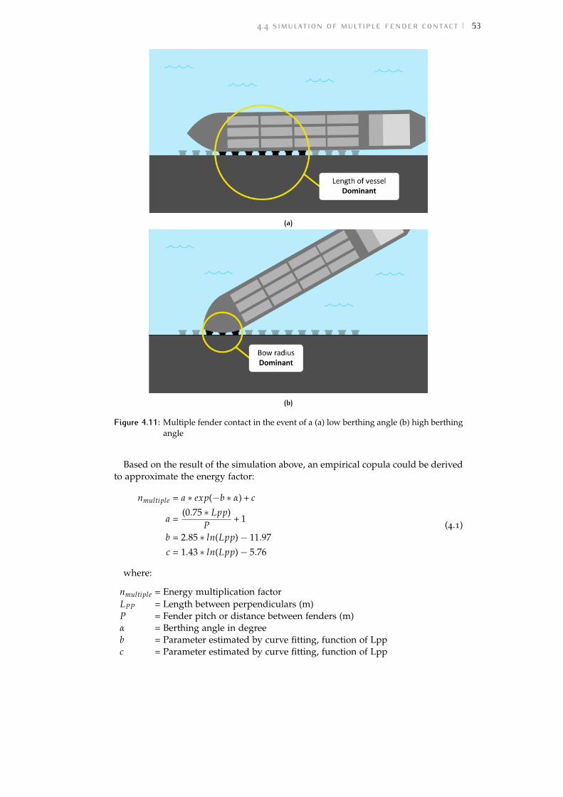
4.4 simulation of multiple fender contact 53

(a)

(b)

Figure 4.11: Multiple fender contact in the event of a (a) low berthing angle (b) high berthingangle

Based on the result of the simulation above, an empirical copula could be derivedto approximate the energy factor:

nmultiple = a ∗ exp(−b ∗ α) + c

a =(0.75 ∗ Lpp)

P+ 1

b = 2.85 ∗ ln(Lpp)− 11.97

c = 1.43 ∗ ln(Lpp)− 5.76

(4.1)

where:

nmultiple = Energy multiplication factorLPP = Length between perpendiculars (m)P = Fender pitch or distance between fenders (m)α = Berthing angle in degreeb = Parameter estimated by curve fitting, function of Lppc = Parameter estimated by curve fitting, function of Lpp

4.5 result of reliability analysis 54

4.5 result of reliability analysisThis section presents the results of the reliability-based assessment, e.g. failureprobability and to what extent the design variables influence the fender reliability.The reliability level of the fenders selected according to the deterministic approach(Table 3.3) was assessed using FORM and Monte Carlo. The following equationgives the limit-state function, which was used for the reliability assessment:

G = nmultiple ∗ Ecv ∗MF ∗VF ∗ TF− 1/2 ∗M ∗ v2 ∗ Ce ∗ Cm (4.2)

Table 4.6 summarizes the distribution families used to describe the uncertaintiesof the design variables. Other necessary information, such as selected fenders, nau-tical depth and distance between fenders, are described in Chapter 3.

Table 4.6: Distribution of the stochastic variablesVariables Distribution Parameters

Velocity Weibull 4.38 cm/s Scale 1.7 cm/s ShapeDisplacement Uniform 8000 ton Lower bound 260,000 ton Upper boundAngle Gamma 1.19o Scale 0.27o ShapeMF Normal 1 Mean 0.033 Std devTemperature Normal 15oC Mean 5oC Std dev

4.5.1 Single Fender Contact

A super cone fender with a rated energy capacity of 1950 kNm and a height 1.6m was selected based on the deterministic approach. The reliability levels of thisfender based on the FORM and Monte Carlo analysis are presented in Table 4.7. Itcould be seen that for the single fender contact scenario and independent variables,the approximate reliability level is 3.64. Whereas, when the variables are negativelycorrelated, the reliability level increases to 4.88.

The result, therefore, shows that the failure probability decreases significantlywhen the dependency between design variables is taken into account. This decreaseis due to the lower likelihood of having a large vessel with a high berthing velocitywhen both variables are negatively correlated. Furthermore, as can be seen in Ta-ble 4.7, the FORM results from three different tools produce the same value. On theother hand, it appears that the failure probability of FORM is slightly higher com-pared to the Monte Carlo result. This slight difference is due to the slight outwardcurvature of the limit state function in the standard normal space that is linearizedin FORM analysis.

Table 4.7: Probability of failure of a single fender per arrival (Ecv=1950 kNm)

MethodIndependent Dependent

Pf β Pf β

Monte Carlo∗ (1.06± 0.19) ∗ 10−43.70 (1.56± 0.23) ∗ 10−7

5.06

FORM (FERUM) 1.35 ∗ 10−43.64 - -

FORM (Prob2B) 1.35 ∗ 10−43.64 - -

FORM (i HL-RF) 1.35 ∗ 10−43.64 5.30 ∗ 10−7

4.88

*) Confidence interval of 95%

Sensitivity factors and design points

Table 4.8 and Table 4.9 show the sensitivity factors and design points for the inde-pendent and dependent cases, respectively. For the independent case, the sensitivityfactor is the largest for the velocity (0.94), indicating that the uncertainty of berthing


velocity largely dominates the uncertainty of the limit-state function. This findingis consistent with the findings of Versteegt [2013] and Yamase et al. [2010].

Table 4.8: Sensitivity factors α and design points for independent case (single fender contact)

VariablesIndependent

unitα Design point

Velocity 0.94 15.07 cm/sDisplacement 0.32 228,600 tonAngle 1.85*10

-40.24

o

Manufacturing tolerance -0.057 0.99 [-]Temperature 0.014 15.27

oC

The sensitivity factors for the dependent case is given in Table 4.9. For the caseof dependent variables, the importance factor (γ) is used instead of the sensitivityfactor (α) to represent the contribution of each stochastic variable in the originalspace. When the design variables are uncorrelated, the value of γ equals to α.The value differs when the variables are dependent since the effect of dependencemight amplify or reduce the contribution of the variables in the original space. Theresult shows that the γ-value of the velocity is the highest compared to other designvariables, followed by the displacement in the second place.

Table 4.9: Sensitivity factors α and design points for dependent case (single fender contact)

VariablesDependent

unitα γ Design point

Velocity 0.70 0.83 14.97 cm/sDisplacement 0.71 0.55 230,530 tonAngle 0.0001 8.68*10

-50.20

o

Manufacturing tolerance -0.068 -0.053 0.99 [-]Temperature 0.018 0.014 15.44

oC

The use of Vine-copula might cause unexpected local minima or maxima in thejoint probability density, which is the condition where the neighbourhood of thedesign point does not significantly contribute to the failure probability Kiureghian[2005]. Therefore, besides performing Monte Carlo to confirm the FORM result,it is also suggested to check the results by plotting the joint distribution and thelimit state function to ensure that the design points are the global solution, notthe local one. Figure 4.12 shows the joint distributions plotted for each pair of thedependent variables. The figure shows that the design points are not located in thelocal maxima or minima since its neighbourhood contributes to the probability offailure.

In conclusion, berthing velocity is the most governing variable for single fendercontact. Another variable with a substantial contribution to the variance of thelimit-state function is displacement. The sensitivity factors for other variables areclose to zero, indicating their negligible contributions to the limit-state function’suncertainty.


Figure 4.12: The joint probability density of the dependent variables around design pointsfor single fender contact

4.5.2 Multiple Fender Contact

The deterministic approach results in the selection of a fender with a rated energycapacity of 1140.4 kNm and a height of 1.4 m in the event of multiple fender contact.Table 4.10 gives the result of the reliability assessment of this selected fender. Theresult shows that the failure probability of this fender is much lower than that ofsingle fender contact, even though this fender has a smaller size and rated energycapacity. This is because, in the case of multiple fender contact, several fenders worktogether to absorb kinetic energy, providing higher energy absorption capacity and,thus, increasing the reliability of the fender system. The failure probability drops to2.10

−7 for the independent case and decreases, even more, to order of magnitude10

-12 when the effect of dependence is taken into account.

Table 4.10: Probability of failure per arrival for multiple fender contact case (Ecv=1140.4kNm)

MethodIndependent Dependent

Pf β Pf β

Monte Carlo∗ (4.30± 1.33) ∗ 10−85.20 (1.62± 1.27) ∗ 10−12

6.96

FORM (FERUM) 2.09 ∗ 10−75.06 - -

FORM (Prob2B) 1.94 ∗ 10−75.07 - -

FORM (i HL-RF) 2.20 ∗ 10−75.05 2.99 ∗ 10−12

6.88

*) Confidence interval of 95%

Sensitivity factors and design points

Table 4.11 presents the sensitivity factors and design point for the independentcase. The result shows that the berthing angle is still the most dominant variable.However, the result shows that now the contribution of berthing angle becomesmuch more important in the event of multiple fender contact as its sensitivity factorincreases to 0.33. This increase is related to the fact that the number of fenders incontact with vessels is influenced by the berthing angle.


Table 4.11: Sensitivity factors α and design points for independent case (multiple fendercontact)

VariablesIndependent

unitα Design point

Velocity 0.91 19.88 cm/sDisplacement 0.25 235,800 tonAngle 0.33 0.91

o

Manufacturing tolerance -0.07 0.99 [-]Temperature 0.02 15.44

oC

Table 4.12 presents the importance factor (γ) for the dependent case. The berthingvelocity still has the strongest influence on the variance of the limit-state function inthe original space, which is followed by displacement in the second place. The jointprobability density around the design points in the original space is illustrated inthe Figure 4.13. It could be seen from the figure that the limit-state function in thevelocity-angle space is quite non-linear. However, the reliability results presentedin Table 4.10 shows this non-linearity does not significantly influence the accuracyof FORM as the difference between FORM and Monte Carlo results is fairly low.

Table 4.12: Sensitivity factors α and design points for dependent case (multiple fender con-tact)

VariablesDependent

unitα γ Design point

Velocity 0.67 0.77 20.01 cm/sDisplacement 0.64 0.57 235,766 tonAngle 0.36 0.28 0.85

o

Manufacturing tolerance -0.0799 -0.062 0.98 [-]Temperature 0.021 0.016 15.70

oC

Figure 4.13: The joint probability density of the dependent variables around design pointsfor multiple fender contact

4.6 distribution of kinetic energy and fender capacity 58

4.6 distribution of kinetic energy and fendercapacity

This section presents the distribution of kinetic energy and fender capacity thatwere derived through a Monte Carlo simulation. Figure 4.14 shows distributions ofthe kinetic energy and fender capacity for the single fender contact berthing proce-dure. The figure on the left shows the distributions where the load variables areindependent of each other. In comparison, the right figure shows the distributionswhere the load variables are negatively correlated.

Figure 4.14: The distribution of the load and resistance for single fender case (Ecv=1950

kNm)

Distribution fitting was then performed for the derived distributions, for whichthe results are presented in Table 4.13. The kinetic energy seems to follow the samedistribution as the berthing velocity, which is the Weibull distribution. On the otherhand, the fender performance follows the same distribution as the manufacturingtolerance, which is the Normal distribution. The results, therefore, suggest that thedistributions of kinetic energy and fender performance reflect the distribution oftheir basic variables.

Furthermore, the result reveals that the uncertainty of kinetic energy is muchhigher compared to the uncertainty of fender performance. Also, the standarddeviation of the kinetic energy decreases when the negative dependence betweenthe variables is taken into account. This decrease could be explained by the fact thatthe extreme kinetic energy occurs less as large vessels tend to have lower berthingvelocities. According to Roubos et al. [2016], the uncertainty in kinetic energy couldfurther be reduced by applying maxima distribution.

Table 4.13: Distribution families of the kinetic energy and fender capacity for the case ofsingle fender contact

Independent case

Variables DistributionPar1

Par2

µ(kNm)

σ(kNm)

c.o.v

Kinetic Energy Weibull 87.96 0.70 111.34 165.45 1.49

Fender Capacity Normal 1962.50 72.50 1962.50 72.50 0.04

Dependent case

Variables DistributionPar1

Par2

µ(kNm)

σ(kNm)

c.o.v

Kinetic Energy Weibull 69.96 0.98 70.79 78.42 1.10

Fender Capacity Normal 1962.50 72.50 1962.50 72.50 0.04

Figure 4.15 presents the distribution of fender capacity for the multiple fendercontact berthing procedure. It should be noted that the effect of multiple fendercontact only alters the distribution of the fender capacity, whereas the distribution

4.7 discussion 59

of the kinetic energy remains the same. The figure shows that the distributions ofthe berthing angle and vessel size significantly influence the tail of fender capacitydistributions. Moreover, it is found that these empirical distributions do not seemto fit any known parametric distribution families.

Figure 4.15: Distribution of fender capacity in the event of multiple fender contact(Ecv=1140.4 kNm)

4.7 discussion

4.7.1 How safe is the fender designed according to PIANC 2002 guideline?

This section discusses how safe is the fender system designed using PIANC [2002].Figure 4.16 demonstrates the reliability of the selected fenders compared to thereliability targets proposed by a sub-group of PIANC WG211 (see Table 5.2), whichis based on ISO2394 (2015).

Figure 4.16: Illustration of the reliability of the selected fenders compared to the reliabilitytargets proposed by PIANC WG211

The result shows that the reliability of the fender design is below the prescribedreliability target when the load variables are independent of each other, and onlyone fender absorbs the entire kinetic energy (single-independent case). The resultedfender design is safe when the effect of negative dependence between the vessel sizewith berthing velocity and berthing angle is taken into account. However, it shouldbe noted that this negative dependence does not always exist, as it depends heavily

4.7 discussion 60

on the local port condition. In some terminals, the variables are independent ofeach other. Therefore, the appropriateness of the existing PIANC guidelines for asingle fender contact type of berthing is still questionable.

On the other hand, for the case of multiple fender contact and independent vari-ables case, the reliability of the selected fender is within the range of the prescribedreliability targets. For the case of Port of Rotterdam, where multiple fenders are ac-tivated during berthing, and the negative dependence exists between the variables,the reliability of the selected fender is far above the required reliability targets (over-designed).

Finally, based on the results presented in Figure 4.16 above, it could be concludedthat the PIANC’s method is sufficiently safe to use for the multiple fender contactberthing procedure. For the case of single fender contact, it is recommended toassign a higher safety factor or to use a higher design berthing velocity, especiallywhen the failure of the fender results in a significant failure consequence. Fur-thermore, neglecting the negative dependence between variables might lead to aconservative fender design.

4.7.2 What if the Nataf transformation was used instead of the Rosenblatt?

In this study, the dependence between berthing velocity, berthing angle, and vesseldisplacement was modelled using the Rosenblatt transformation. Actually, besidesthe Rosenblatt transformation, the Nataf transformation could also be used to trans-form the random variables into a standard normal space and vice versa.

The Nataf transformation is considered more practical in most reliability cases.According to Kiureghian [2005], there are two reasons why: first, it only requiresthe correlation coefficient of the random variables and their coefficient of variation,whereas, for the Rosenblatt transformation, the joint cumulative distribution of thevariables is needed. The second reason is that the transformation to the standardnormal space is simple and does not depend on the ordering of the random vari-ables. Hence, the Nataf transformation is mostly implemented in the probabilistictools such as FERUM.

However, the Nataf transformation has several limitations. Firstly, since the Nataftransformation assumes Gaussian copula, it is therefore not able to accurately ap-proximate non-normal marginal distributions, especially those with a large coeffi-cient of variation (e.g. > 0.5). Moreover, the Nataf transformation is well definedif and only if the copula of the transformed random vector is Gaussian copula Le-brun and Dutfoy [2009]. In this thesis, the marginal distributions of the dependentvariables are not Normal and they have a relatively high coefficient of variation(> 0.5). Moreover, the joint distributions of those variables are asymmetrical andthus, better modelled using the Archimedean copulas. Due to these reasons theNataf transformation is not suitable for this thesis.

Table 4.14 compares the reliability of a fender system computed using the VineCopula method with that computed using the Nataf transformation. The resultsare then plotted in Figure 4.17. It can be seen from the results that the reliabil-ity level of the fender computed using the Nataf transformation is slightly highercompared to the actual reliability obtained using the Vine Copula FORM algorithm.In other words, the reliability of the fender will be over-estimated when the Nataftransformation is used, particularly for the case of Port of Rotterdam.

4.7 discussion 61

Table 4.14: Reliability analysis results for Rosenblatt and Nataf transformations for single-dependent case

Rated capacity(Ecv) (kNm)

Rosenblatt transformation(Vine Copula)

Nataf transformation

β Pf β Pf1140 3.79 7.53 ∗ 10−5

4.18 1.42 ∗ 10−5

1300 4.04 2.67 ∗ 10−54.47 3.89 ∗ 10−6

1500 4.32 7.80 ∗ 10−64.80 7.89 ∗ 10−7

1700 4.58 2.32 ∗ 10−65.10 1.66 ∗ 10−7

1820 4.75 1.01 ∗ 10−65.27 6.67 ∗ 10−8

2175 5.15 1.30 ∗ 10−75.73 4.81 ∗ 10−9

2330 5.32 5.18 ∗ 10−85.92 1.61 ∗ 10−9

2580 5.57 1.27 ∗ 10−86.20 2.82 ∗ 10−10

Figure 4.17: The reliability of a fender system computed using Rosenblatt and Nataf trans-formations

We can understand better the difference by looking at Figure 4.18. It could beseen from the figure that large vessels with high berthing velocity (shown as orangedots) were generated more for the Gumbel copula than for the Gaussian Copula,due to the tail dependence. In Gumbel copula, the dependence is stronger for onetail (Small vessels with higher velocity) than the other tail (Large vessels with lowervelocity), where it is not the case for the Gaussian copula. It thus explains whythe failure probability is underestimated when the Gaussian copula is assumed.Due to that reason, it is hence crucial to choose the right transformation and jointdistribution when modelling dependence between the random variables; otherwise,the estimated reliability level might not be accurate.

4.8 conclusion 62

Figure 4.18: Monte Carlo simulation for Gaussian and Gumbel Copula

4.8 conclusionThe following points summarize the most important findings of this chapter, whichalso could be used to answer the questions given at the beginning of this chapter:

• The results of the distribution fitting show that the distribution of berthingvelocity follows the Weibull distribution, whereas the berthing angle followsthe Gamma distribution. The results are presented in Table 4.6.

• The result of berthing simulation shows that a low berthing angle berthingprocedure is favourable for a fender system as more fenders will be activatedand thus, reducing the load exerted to the individual fender. In other words,taking into account the effect of multiple fender contact will increase the reli-ability of a fender system. Moreover, it is observed that the value of energymultiplication factor (nmultiple) is influenced mainly by the vessel length forthe parallel type of berthing. Whereas, the bow radius governs the value forhigh berthing angles. The effect of berthing angle in governing nmultiple isillustrated in Figure 4.11.

• The data-set of container vessels shows that vessel size is negatively correlatedwith berthing angle and berthing velocity (see Figure 4.7). This negative corre-lation significantly reduces the calculated failure probability and therefore, en-hancing the computed reliability of a fender system. Consequently, a smallerfender size and capacity is required when the effect of negative correlation istaken into design consideration. It is also important to model the dependencestructure between the random variables appropriately. For instance, in this

4.8 conclusion 63

thesis, the dependence was modelled using a Vine copula. Using the Natafdistribution, on the other hand, could over-estimate the reliability of a fendersystem (see Table 4.14).

• The results of FORM reveal that the berthing velocity has the highest impor-tance factor, which means that the uncertainty of berthing velocity has thehighest contribution to the failure of a fender system. This finding is alignedwith the findings of the earlier studies done by Ueda et al. [2003], Yamaseet al. [2010], and Versteegt [2013]. Besides the berthing velocity, vessel dis-placement also has a substantial contribution to the uncertainty of the limit-state function. However, the contribution of the displacement is not as high asthe contribution of the velocity. On the other hand, the influence of berthingangle becomes vital only in the case of multiple fender contact.

• The uncertainty of the berthing kinetic energy is far higher compared to theuncertainty of fender performance Figure 4.14. Therefore, it could be con-cluded that the uncertainty of the kinetic energy has the most dominant influ-ence on the failure of a fender system. Moreover, the distribution of kineticenergy follows the same distribution as the berthing velocity, which is theWeibull distribution. Whereas, the distribution of fender performance followsthe Normal distribution.

• The results of the reliability-based assessment Figure 4.16 shows that the de-terministic method of PIANC guidelines is appropriate for the multiple fendercontact type of berthing. Whereas, in the event of single fender contact, the re-liability of the design is lower than the reliability target prescribed by PIANCWG211.

5 D E R I VAT I O N O F PA R T I A L S A F E T YFA C TO R S

One of the most common methods for designing a structure is to assign a partialsafety factor to the load and resistance variables, commonly known as the semi-probabilistic method. This method allows designers to achieve the intended reli-ability without having to perform a complex full-probabilistic calculation such asMonte Carlo or FORM. Due to its practicality, this method will be implemented inthe new fender design guidelines. This chapter shows how partial safety factorscould be derived using the output of the reliability-based assessment.

5.1 method

5.1.1 Partial Safety Factor for Kinetic Energy and Fender Capacity

The theoretical background of the partial safety factor is explained in Section 2.9.Essentially, the idea of this method is to design a structure such that a certaincharacteristic value of the capacity divided by its partial safety factor is higher thanthe characteristic value of the load effect multiplied by its partial factor:

EFender;kar

γEFender

≥ γEk Ek;kar (5.1)

where:

EFender;kar = Characteristic value of fender absorption capacity (kNm)γEFender = Partial safety factor for fender capacity (-)Ek;kar = Characteristic value of berthing kinetic energy (kNm)γEk = Partial safety factor for kinetic energy (-)

The question now is what are the appropriate values of partial safety factors suchthat the condition described in Equation 5.1 is fulfilled given the prescribed targetreliability. This question was solved by finding the design values of fender capacityand kinetic energy for the target reliability at FORM design points. The partialsafety factors then were determined using the following equations:

γEFender =EFender;kar

EFender;d= ��Ecv ∗MFkar ∗VFkar ∗ TFkar ∗ nmultiple;kar

��Ecv ∗MFd ∗VFd ∗ TFd ∗ nmultiple;d

γEk =Ek;d

Ek,kar=

0.5 ∗Md ∗ v2d ∗ Cmd ∗ Ced

0.5 ∗Mkar ∗ v2kar ∗ Cmkar ∗ Cekar

(5.2)

where:

EFender;d = Design value of the fender absorption capacity at FORM design points (kNm)Ek;d = Design value of the kinetic energy at FORM design points (kNm)

It should be noted that the fender rated capacity (Ecv) in Equation 5.2 is a deter-ministic parameter and hence, could be removed from the equation. Consequently,the value of γEFender is only influenced by the manufacturing tolerance and uncer-tainties related to the rubber properties. Consequently, the partial factors derived

64

5.1 method 65

in this thesis are only valid if the performance of the fender aligns with the productspecifications of the fender. Furthermore, the uncertainty of fender capacity alsodepends on the energy multiplication factor (nmultiple) for multiple fender contactberthing procedure.

Figure 5.1 presents the flow-chart of the partial safety factor derivation. The firststep is to specify reliability targets for the fender system, for which the reliabilitytargets proposed by a sub-group of PIANC WG211 was used in this thesis. Thepartial safety factors were then determined based on the values of the basic variablesat FORM design points and the characteristic values. This calibration aims to ensurethat a structure designed using the partial safety factor has a reliability level closeto the prescribed target reliability. Hence, it is critical to ensure that the reliabilitylevel for the representative structure is close to the target reliability at FORM designpoints.

Figure 5.1: Flowchart of the derivation of partial safety factor

5.1.2 Partial Safety Factor for Reaction Force

Besides the berthing energy, the reaction force generated by fenders is also relevantfor the design of berthing structures and fender system components (e.g. paneland chains). Therefore, the partial safety factors for the reaction force were derivedin this thesis. Similar to Equation 5.2, the partial factors for reaction force can bedetermined using the following equation:

γF =Fd

Fkar(5.3)

where:

γF = Partial safety factor for reaction forceFd = Design value of reaction force (kN)Fkar = Characteristic value of reaction force (kN)

However, the method used to determine the design value of reaction force isdifferent from the method used for energy. As explained previously, the design

5.1 method 66

values of kinetic energy and fender capacity were obtained from FORM designpoints. Whereas, the design value of reaction force was derived from its distribution.Figure 5.2 shows how the safety factors for reaction force was determined in thisthesis.

Figure 5.2: Flow-chart of the partial safety factor derivation for reaction force

This partial factor could be seen as the safety factor accounts for the uncertaintyrelated to velocity factor, manufacturing tolerance, and the exponential increase ofthe reaction force when the fender rated deflection is exceeded.

Characteristic Value

For cone fenders, a small fender deflection already leads to a generation of therated reaction force (Rcv) as shown in Figure 5.3. Consequently, the characteristicand maximum values of the reaction force will be more or less equal to the Rcv.Therefore, it is reasonable to use the rated reaction force as the characteristic valueto derive partial safety factors.

However, there is another aspect that should be taken into account in determin-ing the design reaction force, which is the possibility of having an extremely lowtemperature. For a rubber fender, the temperature factor will rise to 1.2-1.5 for atemperature below −10oC. This case becomes relevant for the design of berthingstructures in countries with a reasonably low temperature such as Norway. This ef-fect, therefore, was taken into account in this thesis by adjusting the rated reactionforce (Rcv) with a temperature factor corresponding to a characteristic temperature(tkar), for which tkar has an exceedance probability of 5% per year. The characteristicforce thus could be written as:

Fkar = Rcv ∗ TF(tkar); where P(t ≤ tkar) = 0.05 (5.4)

Design Value

The design value was determined based on the Load and Resistance Factor Designapproach (LRFD), therefore. the kinetic energy is considered as the dominant loadfor the design of berthing structure. A sensitivity factor of α = −0.7 was thereforeapplied as recommended by the Eurocode 1990. The design reaction force, therefore,equals to:

Fd = F−1(φ(−0.7 ∗ βt)) (5.5)

where φ is the cumulative distribution function of standard normal variable andβt is the reliability target as prescribed in Table 5.2.

Translating Kinetic Energy to Reaction Force

As explained in Section 2.1.2, the kinetic energy can be translated to reaction forceusing the performance curve. Figure 5.3 shows the relation between kinetic energy

5.1 method 67

absorbed by a fender and reaction force it generates. This relationship was used inthis thesis to derive the reaction force distribution (step 2 in Figure 5.2).

Figure 5.3: Energy-Reaction curve

Moreover, since the reaction force peaks twice (at 35% and 72% deflection), therated force (Rcv) was used when the fender deflection is higher than 35%. Therefore,reaction force corresponding to the absorbed berthing energy could be computedusing the following equation:

F =

{Rcv if δ ≥ 35%2 ∗ 10−7E5 − 5 ∗ 10−5E4 + 0.0051E3 − 0.288E2 + 8.1465E + 7.08 if δ < 35%

(5.6)

where E is the kinetic berthing energy absorbed by a fender (kNm) and δ is thefender deflection (%). In the case of multiple fender contact, one fender with themaximum reaction force was chosen as the representative for the fender system.

Furthermore, the actual reaction force is influenced by the surrounding tempera-ture, production tolerance, velocity, and angle of berthing. Therefore, the influencefactors must be applied to the computed reaction force:

Factual = F ∗MF ∗VF ∗ TF ∗ AF (5.7)

5.1.3 Reliability target

In the semi-probabilistic method, a structure is designed based on a certain accept-able probability of failure. One way to represent the acceptable failure probabilityis by using reliability target index. Table 5.1 presents target reliability indexes fordifferent consequence classes proposed by a subgroup of PIANC WG211. The val-ues in the table were derived based on ISO2394. It should, however, be noted thatthese reliability targets are not yet the final values.

5.1 method 68

Table 5.1: Annual reliability targets for different consequence classes proposed by a sub-group of PIANC WG211

Reference Period 1 yearConsequence class A B C DFailure consequence Negligible Some Considerable HighBeta target (βtre f =1year) 3.7 4.2 4.4 4.7

The failure probability corresponding to a certain target reliability index could becomputed as:

Pf = φ(−βt) (5.8)

where φ is the cumulative distribution function of the standard normal distribution.Furthermore, one needs to be aware that a target reliability is always tied to a

certain reference period. For instance, the reliability targets in Table 5.1 are specifiedfor 1-year reference period. It is possible to convert the failure probability associatedwith a certain reference period, to different reference periods (e.g. 1-year or persingle berthing event) using the following formula:

Pf ;tre f= 1− (1− Pf ;singlearrival)

n (5.9)

where:

Pf ;tre f= the probability of failure in the interval [0,tre f ]

Pf ;singlearrival = the probability of failure per single arrivaln = Number of events during the reference period

Figure 5.4 shows a relation between berthing frequency per year and its corre-sponding reliability target index.

Figure 5.4: Reliability target index as a function of berthing events per year

Given that there are 100 berthing arrivals per year in a container berth in Portof Rotterdam, the reliability targets per single arrival corresponding to the annualreliability target (Table 5.1) are given in Table 5.2. These values will be used toderive the partial safety factor in this chapter.

5.2 derivation of partial safety factors for kinetic energy and fender capacity 69

Table 5.2: Reliability target (per berthing arrival) used for the calculation of partial safetyfactors

Class Reliability target (βt) Probability of failureA 4.75 1.08*10

−6

B 5.15 1.33*10−7

C 5.32 5.41*10−8

D 5.57 1.30*10−8

5.2 derivation of partial safety factors for ki-netic energy and fender capacity

This section presents the derivation of partial safety factors for the reliability targetsspecified in Table 5.2. In addition, the characteristic and design values are alsogiven.

5.2.1 Design Values

The design values of the kinetic energy for the prescribed reliability targets are pre-sented in Table 5.3. As explained in the previous section, the design values weredetermined based on the design points of the basic variables obtained from FORManalysis (see Appendix B for the complete results). The result shows that the de-sign points for independent cases are significantly higher than the dependent cases,implying that larger fenders are needed when the load variables are independentof each other.

Table 5.3: Design values of kinetic energy for the prescribed target reliability

CasesEk,d (kNm)

βt =4.75 βt =5.15 βt =5.32 βt =5.57

Single-Independent 3669 4382 4698 5214

Single-Dependent 1935 2319 2488 2756

Multiple-Independent 3171 3822 4113 4600

Multiple-Dependent 1521 1845 2005 2242

Table 5.4 displays the design values of the fender absorption capacity (EFender;d) asa function of the fender rated energy (Ecv). Recall that Ecv is a deterministic param-eter and thus, does not influence the results of the partial safety factor. Therefore, itis better to write the design value as a function of Ecv rather than using its nominalvalue so it can be cancelled out later when deriving the partial safety factor (seeEquation 5.2).

The design value of resistance usually decreases for a higher reliability target.However, a slight increase in design value is observed for the single-independentcase. This increase can be explained by the fact that the fender capacity is influencedby the velocity factor, whose value is proportional to the berthing velocity. Thereforethe design value of the fender capacity will increase as the design berthing velocityalso increases for higher reliability targets.

5.2 derivation of partial safety factors for kinetic energy and fender capacity 70

Table 5.4: Design values of fender capacity for the prescribed target reliability

CasesEFender;d (kNm)

βt=4.75 βt=5.15 βt=5.32 βt=5.57

Single-Independent 1.07 Ecv 1.07 Ecv 1.07 Ecv 1.08 EcvSingle-Dependent 1.07 Ecv 1.07 Ecv 1.07 Ecv 1.07 EcvMultiple-Independent 3.22 Ecv 3.19 Ecv 3.19 Ecv 3.18 EcvMultiple-Dependent 3.55 Ecv 3.48 Ecv 3.45 Ecv 3.42 Ecv

5.2.2 Characteristic Values

Eurocode defines characteristic value as a value with an intended probability of notbeing exceeded by a more extreme value during some specific reference period. Inthis thesis, the characteristic value of the variables and its associated exceedanceprobability are presented in Table 5.5. It should be noted that the exceedance prob-ability specified in Table 5.5 corresponds to the exceedance probability per singlearrival, which is proposed by a subgroup of PIANC WG211. Table B.5 lists the coef-ficients and influence factors associated with the characteristic values in Table 5.5.

Table 5.5: Description of the characteristic values

VariablesExceedanceProbability

CharacteristicValue

Velocity* 0.2% 15.44 cm/sDisplacement** 0% 260,000 tonAngle 5% 0.91o

Manufacturing Tolerance 50% 1

Temperature 50% 15oC*)Corresponding to an exceedance probability of 2% during a reference period of 1 year

**)The displacement of the largest vessel

The characteristic kinetic energy (Ek;kar) and fender capacity (EFender;kar) were thencomputed based on the characteristic values of the random variables presented inTable 5.5. The results are:

Ek,kar = 2460 kNmEFender;kar = 1.08 Ecv kNm (For single fender contact)EFender;kar = 3.30 Ecv kNm (For multiple fender contact)

The characteristic value of the fender capacity for single fender contact is differentfrom the value for multiple fender contact. The difference is due to the contributionof energy multiplication factor (nmultiple).

5.2.3 Partial Safety Factors

Once the design and characteristic values obtained, the partial safety factors couldbe derived directly using Equation 5.2. Table 5.7 shows the computed partial safetyfactors for the kinetic energy. The result shows that the partial safety factors are sig-nificantly higher when the load variables are independent of each other comparedto when they are negatively correlated. Partial safety factors lower than one arefound for dependent cases, indicating that the design values of the kinetic energyare lower than the chosen characteristic values. Thus, lower characteristic valuesmight be used when variables have negative dependence. In addition, it is foundthat the partial safety factors for multiple fender contact are slightly lower comparedto those of single fender contact.

5.3 sensitivity factors 71

Table 5.7: Partial safety factors for kinetic energyConsequence

classesβt

γEkSingle-

IndependentSingle-

DependentMultiple-

IndependentMultiple-

DependentA 4.75 1.49 0.79 1.29 0.62

B 5.15 1.78 0.94 1.55 0.75

C 5.32 1.91 1.01 1.67 0.81

D 5.57 2.12 1.12 1.87 0.91

Table 5.8 shows the partial safety factors for fender capacity. The results show thatγEFender is in general close to 1, indicating that the uncertainty in fender capacity ismuch lower compared to the uncertainty of kinetic energy. Furthermore, partialsafety factors lower than one are found for multiple-dependent case. This couldbe explained by the fact that the chosen characteristic berthing angle is higher thanthe design berthing angle. Consequently, the characteristic fender capacity is lowerthan the design fender capacity.

Table 5.8: Partial safety factors for fender resistanceConsequence

classesβt

γEFenderSingle-

IndependentSingle-

DependentMultiple-

IndependentMultiple-

DependentA 4.75 1.01 1.01 1.02 0.93

B 5.15 1.01 1.01 1.03 0.95

C 5.32 1.01 1.01 1.03 0.96

D 5.57 1.00 1.01 1.04 0.96

Given the partial safety factors in Table 5.7 and Table 5.8, the necessary fendersize and rated capacity needed to achieve the prescribed target reliability could thenbe determined.

5.3 sensitivity factorsBesides the partial safety factors, it is also essential to find the sensitivity factors(α) of the basic variables. Knowing α-values allows us to determine partial factorsfor reliability targets other than those specified in Table 5.1. Moreover, it could beused to differentiate the dominant variables with the non-dominant variables.Thenon-dominant variables then could be considered as deterministic when derivingpartial safety factors.

Table 5.9 and Table 5.10 present the sensitivity factors of the design variables forsingle fender contact case. The first table presents the sensitivity factors for theindependent case, whereas the second table for the dependent case. The resultshows that berthing velocity and displacement are the only important variables inthe event of single fender contact, indicated by a high α-value.

Table 5.9: Sensitivity factors (α) for single fender contact and independent case

Variablesα

βt=4.75 βt=5.15 βt=5.32 βt=5.57

Velocity 0.95 0.96 0.96 0.96

Displacement 0.31 0.30 0.29 0.28

Angle 0.0002 0.0002 0.0002 0.0002

MF -0.020 -0.018 -0.018 -0.017

Temperature 0.0024 0.0022 0.002 0.002

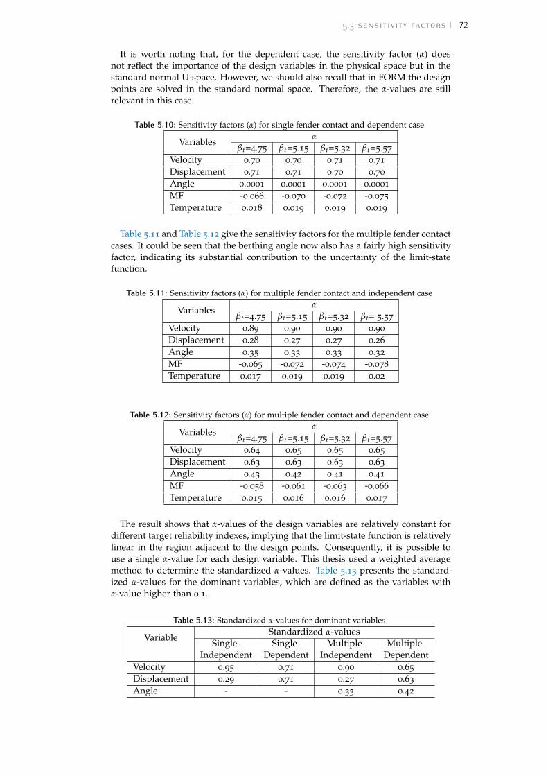
5.3 sensitivity factors 72

It is worth noting that, for the dependent case, the sensitivity factor (α) doesnot reflect the importance of the design variables in the physical space but in thestandard normal U-space. However, we should also recall that in FORM the designpoints are solved in the standard normal space. Therefore, the α-values are stillrelevant in this case.

Table 5.10: Sensitivity factors (α) for single fender contact and dependent case

Variablesα

βt=4.75 βt=5.15 βt=5.32 βt=5.57

Velocity 0.70 0.70 0.71 0.71

Displacement 0.71 0.71 0.70 0.70

Angle 0.0001 0.0001 0.0001 0.0001

MF -0.066 -0.070 -0.072 -0.075

Temperature 0.018 0.019 0.019 0.019

Table 5.11 and Table 5.12 give the sensitivity factors for the multiple fender contactcases. It could be seen that the berthing angle now also has a fairly high sensitivityfactor, indicating its substantial contribution to the uncertainty of the limit-statefunction.

Table 5.11: Sensitivity factors (α) for multiple fender contact and independent case

Variablesα

βt=4.75 βt=5.15 βt=5.32 βt= 5.57

Velocity 0.89 0.90 0.90 0.90

Displacement 0.28 0.27 0.27 0.26

Angle 0.35 0.33 0.33 0.32

MF -0.065 -0.072 -0.074 -0.078

Temperature 0.017 0.019 0.019 0.02

Table 5.12: Sensitivity factors (α) for multiple fender contact and dependent case

Variablesα

βt=4.75 βt=5.15 βt=5.32 βt=5.57

Velocity 0.64 0.65 0.65 0.65

Displacement 0.63 0.63 0.63 0.63

Angle 0.43 0.42 0.41 0.41

MF -0.058 -0.061 -0.063 -0.066

Temperature 0.015 0.016 0.016 0.017

The result shows that α-values of the design variables are relatively constant fordifferent target reliability indexes, implying that the limit-state function is relativelylinear in the region adjacent to the design points. Consequently, it is possible touse a single α-value for each design variable. This thesis used a weighted averagemethod to determine the standardized α-values. Table 5.13 presents the standard-ized α-values for the dominant variables, which are defined as the variables withα-value higher than 0.1.

Table 5.13: Standardized α-values for dominant variables

VariableStandardized α-values

Single-Independent

Single-Dependent

Multiple-Independent

Multiple-Dependent

Velocity 0.95 0.71 0.90 0.65

Displacement 0.29 0.71 0.27 0.63

Angle - - 0.33 0.42

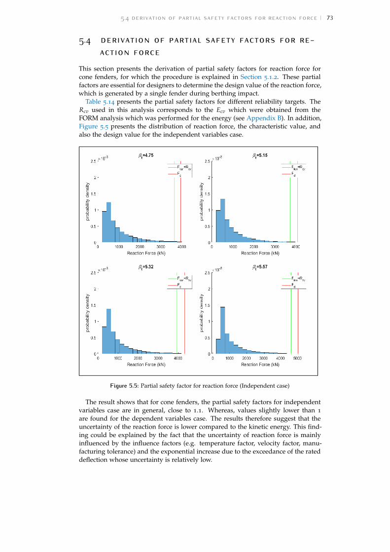
5.4 derivation of partial safety factors for reaction force 73

5.4 derivation of partial safety factors for re-action force

This section presents the derivation of partial safety factors for reaction force forcone fenders, for which the procedure is explained in Section 5.1.2. These partialfactors are essential for designers to determine the design value of the reaction force,which is generated by a single fender during berthing impact.

Table 5.14 presents the partial safety factors for different reliability targets. TheRcv used in this analysis corresponds to the Ecv which were obtained from theFORM analysis which was performed for the energy (see Appendix B). In addition,Figure 5.5 presents the distribution of reaction force, the characteristic value, andalso the design value for the independent variables case.

Figure 5.5: Partial safety factor for reaction force (Independent case)

The result shows that for cone fenders, the partial safety factors for independentvariables case are in general, close to 1.1. Whereas, values slightly lower than 1

are found for the dependent variables case. The results therefore suggest that theuncertainty of the reaction force is lower compared to the kinetic energy. This find-ing could be explained by the fact that the uncertainty of reaction force is mainlyinfluenced by the influence factors (e.g. temperature factor, velocity factor, manu-facturing tolerance) and the exponential increase due to the exceedance of the rateddeflection whose uncertainty is relatively low.

5.5 discussion 74

Table 5.14: Partial safety factors for reaction force (SCN Fender)

βt Rcv TF(tkar)=6oCFkar

(kN)Independent Dependent

Fd(kN)

γFFd

(kN)γF

4.75 3568

1.02

3639 3947 1.08 3518 0.97

5.15 3640 3713 4067 1.10 3601 0.97

5.32 3850 3927 4321 1.10 3825 0.97

5.57 4523 4613 5134 1.11 4529 0.98

It should be noted that the partial factors in Table 5.14 were derived for conefenders. The values of partial safety factors will be higher for cylindrical fenders.However, the partial factor for cylindrical fenders is outside of the scope of thisthesis.

5.5 discussion

5.5.1 Evaluation of the Safety Factors of PIANC [2002]

This section evaluates the safety factors recommended by PIANC [2002] and com-pares them with the partial safety factors derived in this thesis. As explained in Sec-tion 3.3.2, PIANC [2002] introduces abnormal berthing coefficient (Cab) as a globalsafety factor to be applied to the normal kinetic energy. PIANC recommends toassign a global safety factor of 1.5 for the largest container vessel and 2.0 for thesmallest container vessel to the kinetic energy (see Table 2.1). Table 5.15 comparesthe abnormal berthing coefficient suggested by PIANC guideline and the partialsafety factors for kinetic energy derived in this thesis for the independent variablescases. It could be seen that the values of γEk are found to be in the similar range ofthe Cab recommended by PIANC.

Table 5.15: Comparison between Cab and γEk

Consequence CabγEk

Single-Independent Multiple-IndependentLow

1.5-2.0

1.49 1.29

Some 1.78 1.55

Considerable 1.91 1.67

High 2.12 1.87

However, it should be noted that the design philosophy of PIANC [2002] is dif-ferent from the partial safety factor method. In the PIANC guidelines, the safetyfactor is assigned to the ’normal kinetic energy’, which is computed based on thedeterministic values recommended in the guidelines. Whereas, the characteristicvalues are derived from the marginal distribution of the basic variables. The char-acteristic kinetic energy in this thesis is found to be higher than the ’normal kineticenergy’ computed based on the PIANC guidelines (see Table 5.16); this is becausethe characteristic berthing velocity is far higher than the velocity recommended byBrolsma et al. [1977].

Table 5.16: Comparison between the ’Normal’ kinetic energy computed based on the deter-ministic approach of PIANC [2002] and the characteristic kinetic energy derivedin this thesis

MethodDisplacement

(ton)Velocity(cm/s)

Angle(degree)

Kinetic Energy(kNm)

Remarks

Deterministic 260,000 10 1.5 1193 Table 3.3Semi Probabilistic 260,000 15.5 0.9 2460 Table 5.5

5.5 discussion 75

Therefore, it is highly recommended to update the Brolsma’s velocity curve, asalso suggested by Roubos et al. [2016], such that the ’normal kinetic energy’ matchesthe characteristic value. It is further recommended to implement the partial safetyfactor method in the new fender guideline as it has some advantages over the ex-isting global safety factor. For instance, the use of partial safety factor allows engi-neers to allocate an appropriate partial factor according to the intended reliabilitytarget and design assumption (e.g. multiple fender contact) and therefore, an over-designed fender could be avoid.

5.5.2 Verification of the method used to find design values for the case of depen-dent variables

It has been explained in the previous in Section 2.9 that the design values could beapproximated based on the sensitivity factors (α). This method, however, might benot accurate when variables are dependent on each other due to the non-linear iso-probabilistic transformation (e.g. Rosenblatt transformation). Therefore, this doc-ument aims to confirm whether the approximated failure probability determinedusing the α-values matches the intended reliability target (βt).

Figure 5.6: Conceptual illustration of the design points in the standard normal U-space andphysical X-space for dependent variables (The author’s illustration)

Figure 5.6 illustrates the verification process. A FORM analysis was performedfor a fender (single-dependent case), resulting in β∗ = 4.75 and the associated sen-sitivity factors (α∗) and design points (X∗). Those results were then used to ap-proximate the new design values for a different reliability target (e.g. β = 5.15).The new design values were obtained using Equation 2.67, for which the results arepresented in Table 5.17.

Table 5.17: The results of the calculation of the new design points (X)Variables α∗ α∗.(β− β∗) U∗ U X∗ X

Velocity 0.70 0.28 3.32 3.60 14.55 cm/s 15.68 cm/sMass 0.71 0.284 3.38 3.66 229,132 ton 236,047 tonAngle 1.10−4 4.10−5 5 ∗ 10−4 5 ∗ 10−4 0.19o 0.20o

MF -0.066 -0.028 -0.32 -0.34 0.99 0.99

Temperature 0.018 0.008 0.08 0.09 15.41oC 15.45oC

As illustrated in Table 5.17, the design values of velocity, displacement, and angleare higher for the new reliability target, implying that the loads have to be moreextreme or unlikely to reach a failure condition. As these new design loads have asmaller exceedance probability, the failure probability will therefore also be lower.

5.5 discussion 76

However, the question was whether this failure probability is similar to the allow-able maximum probability corresponding with the desired reliability target. Oneway to verify that is by analysing whether the following approximation holds:

P[Z < Z(X)] ∼= φ(−β) (5.10)

The new reliability level (β) represents the exceedance probability of the newlimit-state function Z=Z(X), as illustrated in Figure 5.7. It could be seen from thefigure that the new exceedance probability is smaller than the original failure prob-ability.

Figure 5.7: The exceedance probability of the new limit-state function Z=Z(X) (The author’sillustration)

The value Z(X) was computed according to the new design points (X) given inTable 5.17, for which the result is -381 kNm. The exceedance probability of the newlimit state function P[Z<Z(X)] was then determined by means of Monte Carlo andFORM, for which the results are given in Table 5.18.

Table 5.18: The exceedance probability of the new limit-state function

β φ(−β)FORM Monte Carlo*

P[Z < Z(X)] P[Z < Z(X)] c.o.v5.15 1.30*10

-71.26*10

-75.06*10

-80.09

*) Monte Carlo was performed using 1 million samples

The results show that the exceedance probability obtained from FORM is close tothe intended target reliability, whereas the exceedance probability computed usingMonte Carlo is slightly smaller. The difference between the result of Monte Carloand the target failure probability is due to the non-linear transformation of thedependent variables, however, this difference is fairly small and still acceptable.

Figure 5.8 shows the exceedance probability of the new limit-state function ob-tained from the Monte Carlo simulation and its associated confidence interval, andthe desired failure probability. The result shows that the uncertainty of the MonteCarlo’s failure probability is much smaller compared to its difference with the in-tended target reliability, indicating the convergence of the Monte Carlo result.

Based on the analysis results, it could be concluded that it is safe to use α-valuesto derive design values for dependent variable cases.

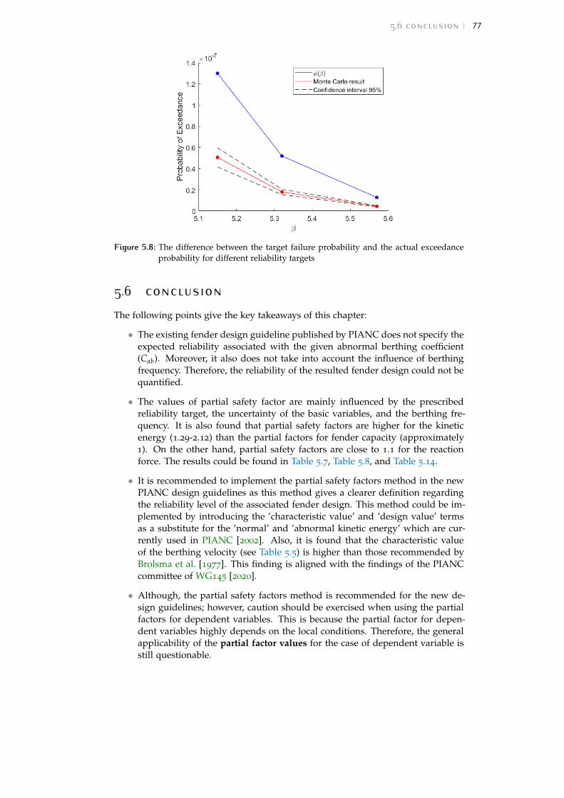
5.6 conclusion 77

Figure 5.8: The difference between the target failure probability and the actual exceedanceprobability for different reliability targets

5.6 conclusionThe following points give the key takeaways of this chapter:

• The existing fender design guideline published by PIANC does not specify theexpected reliability associated with the given abnormal berthing coefficient(Cab). Moreover, it also does not take into account the influence of berthingfrequency. Therefore, the reliability of the resulted fender design could not bequantified.

• The values of partial safety factor are mainly influenced by the prescribedreliability target, the uncertainty of the basic variables, and the berthing fre-quency. It is also found that partial safety factors are higher for the kineticenergy (1.29-2.12) than the partial factors for fender capacity (approximately1). On the other hand, partial safety factors are close to 1.1 for the reactionforce. The results could be found in Table 5.7, Table 5.8, and Table 5.14.

• It is recommended to implement the partial safety factors method in the newPIANC design guidelines as this method gives a clearer definition regardingthe reliability level of the associated fender design. This method could be im-plemented by introducing the ’characteristic value’ and ’design value’ termsas a substitute for the ’normal’ and ’abnormal kinetic energy’ which are cur-rently used in PIANC [2002]. Also, it is found that the characteristic valueof the berthing velocity (see Table 5.5) is higher than those recommended byBrolsma et al. [1977]. This finding is aligned with the findings of the PIANCcommittee of WG145 [2020].

• Although, the partial safety factors method is recommended for the new de-sign guidelines; however, caution should be exercised when using the partialfactors for dependent variables. This is because the partial factor for depen-dent variables highly depends on the local conditions. Therefore, the generalapplicability of the partial factor values for the case of dependent variable isstill questionable.

6 E C O N O M I C O P T I M I S AT I O N

”How safe is safe enough?” is one of the fundamental questions that every engi-neer should have an answer to before designing a structure. Engineers can makea highly safe structure which obviously will lead to a reasonably high cost of in-vestment, or they can also create a cheaper design at the expense of the reliabilityof the structure. Engineers and the project owner hence will always encounter thisdilemma when they decide to build a structure. In essence, the appropriate relia-bility level of a structure depends on the efficiency of the safety measure and thefailure consequence of the structure.

In practice, structures are usually designed to meet a certain safety level, as pre-scribed in the relevant codes or standards. For instance, engineers in Europe usuallycreate their design following the Eurocode. However, the existing codes are mainlyderived for buildings. It is thus unclear whether or not the prescribed reliability tar-gets in the standard are still relevant for structures with different risk-profile. Thegoal of this chapter is to derive the optimum reliability target for fender structurebased on the economical optimisation.

6.1 procedureFigure 6.1 shows the flow-chart of the analysis used for finding the most appropriatereliability target for fender structure. Besides the economic optimization, sensitiv-ity analysis will also be conducted to determine which parameter has a dominantinfluence on the fender’s optimum reliability. In this analysis, the optimum relia-bility level will be derived for the case of single fender contact with independentparameters.

The first step of the analysis is to determine the value of input parameters used forthe calculation, such as interest rate, failure cost, investment cost, and the lifetimeperiod of a fender structure. This study collects relevant data from various sources.For example, this study used the fender’s price provided by Trelleborg, while thestudy of Roubos et al. [2019] was used to estimate the failure cost. When all of thenecessary inputs are defined, one can determine the optimum reliability target byminimizing Equation 2.71. Readers can also find a more detailed elaboration on theconcept of economic optimization in Section 2.10.

78

6.2 result of economic optimisation 79

Figure 6.1: Flowchart of the economic optimization analysis

6.2 result of economic optimisation

6.2.1 Data Analysis

In the economic optimization method, the investment cost (Ci) and capitalized riskcost (CR) are defined as a function of the system’s reliability level. One couldobtain the relationship between fender’s reliability level with the investment costby performing reliability analysis, either Monte Carlo or FORM, for several fenderswhose rated energy capacity and price have already known. Normally, the fender’srated energy is proportional to the reliability level.

Figure 6.2 presents the price of super cone fender (SCN) and cylindrical fender(CYL) as a function of the fender’s reliability level per single arrival. It is clearfrom the figure that the fender’s price increases as the reliability level increases. Inaddition to that, the price of the CYL type of fender is higher than the SCN one, andthus, we can compare the influence of the fender’s price on the optimum reliabilitylevel. With polynomial regression, the price of the fender is approximated using aquadratic function. Equation 6.1 and Equation 6.2 are used to approximate the costof investment for the SCN and CYL type of fender, respectively.

Ci = 2386 ∗ β2 + 146 ∗ β + 6118 (6.1)

Ci = 6268 ∗ β2 − 7395 ∗ β + 11655 (6.2)

Roubos et al. [2019] studied the optimum reliability target indices for the quaywall. In his study, he tried to examine the failure consequence of a quay wall bygathering expert’s opinions on the qualitative and quantitative estimate of the fail-ure consequences. He found that most experts agree that structural failure will notlikely cause significant economic repercussions in large ports. However, a structuralfailure may harm the ports’ reputation, and thus, mitigation measures are essential

6.2 result of economic optimisation 80

Figure 6.2: Prices of fender as a function of reliability level per arrival (Source:Trelleborginternal document)

to prevent failures. The majority of the experts also agree that the failure costs as-sociated with structural failure of a commercial quay wall are in the ranges of e1-5million.

It is not likely that the failure of a single fender will directly lead to marinestructure failure. Therefore, the failure costs of the fender are most likely lowerthan the quay wall. Hence, in this thesis, it is assumed that a fender failure’sconsequence cost is ≤ e1 million. It is further assumed that the probability offatality caused by a single fender failure is extremely small. The influence of failurecosts on the optimum reliability level will be taken into account in the sensitivityanalysis section.

Other parameters whose values need to be defined are interest rate and the designlife-span of a fender. In practice, the design lifetime of a fender is 25 years. As forthe interest rate, according to Miller [2020], the fixed 20-years fixed mortgage in theNetherlands is approximately 2.65-3.4% while Roubos et al. [2019] assumed interestrate of 3% in his study. In this thesis, 3% interest rate thus was also assumed.

6.2.2 Optimum Annual Reliability Level

Figure 6.3 presents the economic optimization results for the super cone fender andcylindrical fender. It could be seen that the optimum annual reliability index forthe super cone fender is 3.47. On the other hand, the cylindrical fender’s optimumreliability index is slightly lower, which is 3.24. The optimum reliability index willdecrease when the cost of investment increases.

It is also observed from the figure that the steepness of the total cost curve isasymmetrical. The steepness on the left side of the graph is mainly influencedby the capitalized risk cost (the red line), while the steepness on the right side isinfluenced by the investment cost (the blue line). The efficiency of safety investmentbecomes less when the reliability level is already larger than 3.2, which means thatspending more in the safety measure will not significantly reduce the probabilityof failure anymore. In the next section, the influence of the parameters on theoptimum reliability level will be examined.

6.3 result of sensitivity analysis 81

(a)

(b)

Figure 6.3: Optimum annual reliability index tre f =25 years, r = 3%, C f = e1 mil for (a) SuperCone Fender (b) Cylindrical Fender

6.3 result of sensitivity analysisThe purpose of sensitivity analysis is to find which parameter that has a significantinfluence on the optimum safety level of a fender. We will perform sensitivityanalysis for interest rate (r), failure cost (C f ), reference period (T), and the numberof berthing arrivals per year. The sensitivity analysis was done by changing oneparameter of interest while keeping the other parameters constant.

Figure 6.4 presents the results of the sensitivity analysis. As expected, the opti-mum reliability level goes up as the failure costs increase. The optimum reliabilitylevel increases exponentially for the low failure cost (≤ e5 million). The increaseis gentler for the higher failure cost. On the other hand, the interest rate has anopposite effect on the optimum reliability index than the failure cost. The opti-mum reliability level will decrease when the interest rate increases, which can beexplained by the fact that the present value of the risk cost will be less for higherinterest rates. The more extended reference period leads to a higher optimum re-liability index. However, the optimum reliability index tends to be constant for areference period longer than 30 years. This is because the capitalized risk cost is

6.4 discussion 82

Figure 6.4: Influence of (a) cost of failure, (b) interest rate, (c) reference period, (d) berthingfrequency per year on the annual reliability index for C f = e1 mil, berthing fre-quency=100 arrivals/year, r=3%, T=25 years

mainly governed by the present value of the consequence cost in the near future.Lastly, the frequency of berthing arrival does not influence the optimum annual re-liability index, but it will slightly influence the optimum reliability index of a singlearrival.

6.4 discussion

6.4.1 Evaluation of the reliability target indices proposed by PIANC WG211

As explained in the previous chapter (see Figure 5.4), a sub-group of PIANC WG211

has proposed several reliability targets for different failure consequences, which areadopted from ISO2394 (2015). In this section, those proposed reliability targets arecompared to the optimum reliability targets derived from the cost-benefit analysis,as presented in Table 6.1. The results of the cost-benefit analysis show that theproposed reliability targets are aligned with the optimum reliability targets derivedfor the Cylindrical fenders. Whereas, the optimum reliability targets for the Conefenders are slightly higher due to the lower marginal cost. Therefore, based onthe results of the economic optimisation, it could be concluded that the reliabilitytargets proposed by the PIANC WG211 are already optimum.

However, it should be noted that the optimum reliability targets derived in thisthesis do not take into account the fatalities and environmental consequences. There-

6.5 conclusion 83

fore, a higher reliability target should be imposed where the failure of a fendersystem leads to fatalities or severe environmental damages.

Table 6.1: The annual reliability targets proposed by PIANC WG211 and the optimum relia-bility targets derived in this thesis for different failure consequences

Class ConsequenceFailure cost(million e)

βtre f =1year

PIANC WG211 SCN Fenders CYL FendersA Low ≤8 3.7 4.0 3.8B Some ≤50 4.2 4.4 4.2C Considerable ≤200 4.4 4.7 4.5D High ≤1500 4.7 5.1 4.9

6.5 conclusionSome important findings of this chapter are:

• The optimum annual reliability target indices is largely influenced by the fail-ure cost and also, the cost of investment. Higher consequence cost will resultin the higher optimum reliability target. On the other hand, the optimum reli-ability target will become lower when the investment cost is more expensive.

• The optimum reliability target for cylindrical fender is slightly lower than thesuper cone fender, as it has a higher investment cost (see Figure 6.3).

• Given that the failure cost of a single fender is e1 million, 100 berthing arrivalsper year and that the design lifetime of the fender is 25 years, the annualoptimum reliability of a super cone fender and cylindrical fender are 3.47 and3.24, respectively.

• The optimum annual reliability target suggested by PIANC WG121 is alignedwith the optimum reliability target found from the economic optimisation asthe analysis shows that the optimum reliability target should be in the rangeof 3.5-4.5 depending on the failure consequences.

7 C O N C L U S I O N A N DR E C O M M E N DAT I O N

This thesis has addressed some critical aspects related to the reliability of a fendersystem. The First Order Reliability Method (FORM) and Monte Carlo simulationwere performed to assess the reliability level of the fenders selected using PIANC[2002] while taking into account the influence of multiple fender contact and nega-tive dependence between the load variables. This thesis is the first study that takesthe effect of multiple fender contact and negative dependence into considerationsince the previous studies by Ueda et al. [2003], Yamase et al. [2010], and Versteegt[2013], assumed a single fender contact and independent variables. Furthermore,this thesis shows how partial safety factors could be derived using the results ofthe level-II probabilistic analysis (FORM). In the last chapter, the optimum reliabil-ity target index was determined through a cost-benefit analysis. During this study,some novel insights related to fender design have been acquired. It is highly recom-mended that these aspects be discussed in future PIANC working groups.

7.1 conclusionThis section presents the answer to the sub-questions and also the main researchquestions formulated in Chapter 1 based on the results of the reliability-based as-sessment performed in this thesis which also summarises the main findings of thisthesis.

1. What are the reliability levels of the fender systems designed using thecurrent PIANC fender design guidelines?

The answer to this question is given in Section 4.5 and discussed specificallyin Section 4.7.1. The result shows that for the single fender contact berthingprocedure, the reliability levels of the fender selected based on PIANC [2002]are 3.70 and 5.06 for independent and dependent variables cases, respectively.Whereas, much higher reliability levels are found for the multiple fender con-tact berthing procedure. The reliability level of the fender system is 5.20 forthe independent variables and 6.88 for the dependent load variables, respec-tively.

2. Do those fender designs meet the reliability targets proposed by PIANCWG211?

If we compare the reliability level of the fenders to the reliability targets pro-posed by PIANC WG211, it is found that the reliability level for the single-independent case (β = 3.70) is below the proposed reliability target. A highercharacteristic berthing velocity, therefore, is recommended to be used for thedesign calculation. On the other hand, the reliability-based assessment resultshows that for the multiple fender contact type of berthing, the reliability ofthe fender design is in the range of the reliability target proposed by PIANCWG211. However, it should be noted that for the multiple fender contact, 3-fender contact was assumed (Figure 3.5). Hence, it could be concluded thatthe existing design method is suitable for the multiple fender contact type ofberthing.

3. How could the dependence between the load variables be modelled?

84

7.1 conclusion 85

A dependence analysis was performed for the container terminal data-set inPort of Rotterdam to answer the question above. It is found that the vesselsize has a negative correlation with berthing velocity (ρ = −0.61) and berthingangle (ρ = −0.54). Furthermore, the result of Kendall’s tau independence testalso confirms the dependence between those load variables. A Vine-copulawas then used to model the dependence structure between those variablesand included in FORM analysis using the algorithm proposed by Jiang et al.[2015].

4. What influence does dependence have on the reliability of a fender system?

The reliability assessment results further show that the negative dependencebetween the load variables could significantly reduce the calculated failureprobability of a fender system, enhancing the calculated reliability of thefender system. This decrease in the failure probability is because the largevessels will tend to have lower berthing angle and velocity when they arenegatively correlated. Therefore, the occurrence probability of extreme kineticenergy will become smaller. Neglecting this negative dependence might leadto an oversized fender design.

5. How could the influence of multiple fender contact be included in the limit-state function?

In the event of multiple fender contact berthing procedure, the kinetic energyexerted by the vessel is absorbed by multiple fenders that are in contact withthe vessel. The proportion of the energy absorbed by those fenders dependson the deflection of each fender. To account for the contribution from severalfenders in contact the energy multiplication factor nmultiple is introduced. Thisfactor depends on the geometry of the vessels and the spacing between fend-ers and can be determined based on geometrical analysis or more advancedsimulation (see Section 4.1.2). For relatively low berthing angles, nmultiple ismainly influenced by the vessel length. On the other hand, for high berthingangles, nmultiple is governed by the bow radius.

6. How significant is the influence of the multiple fender contact on the relia-bility of a fender system?

The multiple fender contact has a favourable influence on the reliability ofa fender system, which is similar to the effect of the negative dependencebetween the load variables. When the influence of multiple fender contactis taken into account, the calculated failure probability of a fender systembecomes significantly lower. Therefore, it is essential to take this favourableeffect of the reasonably low berthing angle and multiple fender contact intoaccount in the design of a fender system; otherwise, the design might becometoo conservative.

7. Which random variable has the most dominant influence on the failure ofa fender system?

This thesis confirms that the uncertainty of berthing velocity has the largestcontribution to the failure of the fender system. This finding is aligned withthe findings of Ueda et al. [2003], Yamase et al. [2010], and Versteegt [2013].Besides the berthing velocity, another variable whose uncertainty has a sub-stantial influence on the variance of the limit-state function is the vessel dis-placement. Whereas, the contribution of berthing angle becomes significantin the event of multiple fender contact.

8. What are the optimum reliability target (βt) for a fender system?

The cost-benefit analysis result shows that the optimum annual reliability tar-get is aligned with those proposed by the sub-group of PIANC WG211, whichis in the range of 3.5-4.5 (depending on the failure consequence). It is also

7.2 recommendations 86

found that the optimum reliability target is mainly influenced by the safetymeasure cost, the cost of failure consequence, and the reference period.

9. What is the appropriate partial safety factors for the kinetic energy, fendercapacity, and reaction force?

Chapter 5 shows how the partial safety factors were derived based on theresults of FORM analysis. In essence, the design points obtained from theFORM analysis were used as the design values for determining the partialsafety factors. It is found that a higher safety factor (1.2-2.2) needs to beassigned to the kinetic energy as its uncertainty dominates the failure of afender system. Whereas, in general, it is found that the partial safety factorsfor fender capacity are approximately 1. On the other hand, the partial safetyfactors for reaction force for cone fenders in general equals 1.1.

Finally, the main research question below could be answered:

”How can the existing fender design approach be improved using thereliability-based design approach and what aspects need to be considered?”

Most of the existing fender design guidelines adopt the deterministic approach inwhich the reliability related to fender engineering is not taken into account. Thisthesis shows how those uncertainties could be incorporated into design consider-ation in order to produce a sufficiently safe fender design. One way to improvethe existing design approach is by implementing the partial safety factor methodto update the current deterministic approach. In the partial safety factor method,the uncertainties of the load variables (e.g. berthing velocity, berthing angle, anddisplacement) are taken into account via the characteristic and design values. Fur-thermore, this method allows fender designers to allocate an appropriate partialfactor according to the intended failure consequence and design assumption (e.g.single/multiple fender contact) and thus, avoiding an oversize fender design. Theberthing frequency is also taken into account into the design consideration throughthe reliability target per berthing arrival.

This thesis has several contributions to both academic research and industrialapplications. In terms of academic contribution, this thesis shows a practical appli-cation of the Vine Copula FORM algorithm developed by Jiang et al. [2015]. Thisthesis further demonstrates how the design points could be determined using theRosenblatt transformation in the event of dependent variables is modelled usingVine copula. The methods were then verified in Section 5.5.2. Whereas, for theindustrial contributions, this thesis manages to show how the influence of multiplefender contact and dependence between the load variables could be integrated intothe design of a fender system. In the earlier studies (e.g. Yamase et al. [2010], Uedaet al. [2003], Versteegt [2013]), the effects of the negative dependence and multiplefender contact were not considered. The results of this thesis show how those ef-fects have a very dominant influence on the reliability of a fender system. Therefore,this thesis could be used by PIANC WG 211 to update the existing design approachof fender systems and help to interpret the berthing records analyzed by PIANCWG145.

7.2 recommendationsThe following recommendations are recommended for future research and the for-mulation of new fender design guidelines:

1. It is recommended to take into account the favourable effects of multiplefender contact and relatively low berthing angles in the design guidelines for

7.2 recommendations 87

the fender system in order to create a more cost-effective fender design. PI-ANC should develop design guidance for parallel berthing as it is still lackingin the existing guidelines.

2. Although PIANC WG145 has collected many data, the available amount ofberthing operation records is still limited. Consequently, it is recommendedto collect new data to confirm correlations between berthing velocity and otherdesign variables.

3. PIANC WG211 should take the effect of negative dependence between theload variables into fender design consideration as it could significantly reducethe required fender size. For instance, we could apply a correction factor tothe characteristic kinetic energy in order to account for the effect of the depen-dence. However, since the dependence between the variables depends heavilyon the local port conditions, it is not easy to formulate a value that could beused for general practice. In fact, consideration of negative dependence be-tween load variables may lead to an inadequate fender design if incorporatedwithout proper justification from site-specific data.

4. In order to improve the results of the reliability-based assessment, it is recom-mended to perform the Second-Order Reliability Method (SORM) to assessthe reliability of the fender system. This is because results of FORM mightnot be accurate when the limit-state function is strongly non-linear, and whenthe dependency between variables is non-linear.

5. Finally, it is recommended to improve the multiple fender contact simulationwhich was used in this thesis. For future research, more variables could beincorporated into the simulation model (e.g. fender pitch, fender size) in orderto gain more insight into what factors determine the contribution of multiplefender contact.

B I B L I O G R A P H Y

Bedford, T. and Cooke, R. (2001). Probabilistic Risk Analysis: Foundations and Methods.Cambridge, Cambridge.

Brolsma, J., Hirs, J., and Langeveld, J. (1977). Paper of fender design and berthingvelocities. PIANC World Congress.

Coastal Development Institute of Technology, . (2019). Guidelines for Design andTesting of Rubber Fender System. Japan.

Cooke, R. (1997). Markov and entropy properties of tree- and vine-dependent vari-ables. American Statistical Association - Proceedings of the Section on Bayesian Sta-tistical Science.

Genest, C. and Favre, A.-C. (2007). Everything you always wanted to know aboutcopula modeling but were afraid to ask. Journal of Hydrologic Engineering(ASCE).

Graler, B., van den Berg, M. J., Vandenberghe, S., Petroselli, A., Grimaldi, S.,De Baets, B., and Verhoest, N. E. C. (2013). Multivariate return periods inhydrology: a critical and practical review focusing on synthetic design hydro-graph estimation. Hydrology and Earth System Sciences.

Hein, C. (2014). Berthing velocity of large container ships. PIANC World Congress.

Iversen, R, P., W, Bruin, P., B, Phan, P., and J, Pyun, S. (2019). A proposed rationalapproach to design of fenders and supporting structures in the united states.LRFD.

Jiang, C., Han, X., Zhang, W., and Ni, B. (2015). A vine-copula-based reliabilityanalysis method for structures with multidimensional correlation. Journal inMechanical Design.

Jianping, L., Dengsheng, W., Xioqian, Z., and Young, S. (2015). On the aggrega-tion of credit, market and operational risks. Review of Quantitative Finance andAccounting.

Jonkman, S., Steenbergen, R., Morales-Napoles, O., Vrijling, J., and Vrouwenvelder,A. (2017). Probabilistic Design: Risk and Reliability Analysis in Civil Engineering.Department of Hydraulic Engineering, Faculty of Civil Engineering and Geo-sciences, TU Delft, Delft.

Kiureghian, A. D. (2005). First- and second-order reliability methods. In Nikolaidis,E., M. Ghiocel, D., and Singhal, S., editors, Engineering Design Reliability hand-book, chapter 14. CRC Press.

Kooij, L. V. D. (2020). Extreme value analysis if complex wave systems. Master’sthesis, Delft University of Technology, Delft.

Kurowicka, D. and Cooke, R. (2006). Uncertainty Analysis with High DimensionalDependence Modelling. Wiley Series in Probability and Statistics, Delft.

Lebrun, R. and Dutfoy, A. (2009). Do rosenblatt and nataf isoprobabilistic transfor-mations really differ? Probabilistic Engineering Mechanics.

Lemaire, M. (2005). Structural Reliability. John Wiley & Sons, Inc., London.

88

BIBLIOGRAPHY 89

Miller, I. (2020). Mortgages in the netherlands. https://www.expatica.com/nl/

housing/buying/your-guide-to-dutch-mortgages-101837/. Accessed: 2020-06-10.

Moss, R. E. S. (2020). Applied Civil Engineering Risk Analysis 2nd ed. Springer, Cham,Switzerland.

PIANC (2002). Guidelines for the design of fender system:2002.

Roubos, A., Groenewegen, L., and Peters, D. J. (2016). Berthing velocity of largeseagoing vessels in port of rotterdam. Marine Structures, 51:202–219.

Roubos, A., Groenewegen, L., Peters, D. J., and Steenbergen, R. (2018). Partial safetyfactors for berthing velocity and loads on matrine structures. Marine Structures,58:73–91.

Roubos, A., Schweckendiek, T., Brinkgreve, R., Steenbergen, R. D. J. M., andJonkman, S. (2019). Finite element-based reliability assessment of quay walls.Georisk:Assessment and Management of Risk for Engineered Systems and Geohazards.

Shibata (2017). Fender Design Manual.

Trelleborg (2018). Fender Application Design Manual.

Ueda, S., Nagao, T., and Okada, T. (2003). Study on reliability-base design methodfor fenders based on form. Proc. of Annual Journal of Civil Engineering in theOcean, JSCE.

Valls, S. S. (2019). A vine-based approach for defining critical infrastructure loads.Master’s thesis, Delft University of Technology, Delft.

Versteegt, G. (2013). Berthing loads in structural design (validation of partial factor.Master thesis, Delft University of Technology.

Vrijburcht, A. (1991). Loads on fender structures and dolphins by sailing ships. Rijkswa-terstaat, the Hague.

WG145, P. (2020). Berthing velocity analysis of seagoing vessels over 30,000 dwt.Technical report, PIANC.

Yamase, S., Ueda, S., and Okada, T. (2010). Reliability design of fender system forberthing ships. PIANC MMX Congress Liverpool UK.

https://www.expatica.com/nl/housing/buying/your-guide-to-dutch-mortgages-101837/

https://www.expatica.com/nl/housing/buying/your-guide-to-dutch-mortgages-101837/

A V I N E C O P U L A G O O D N E S S - O F - F I T

a.1 semi-correlationThe semi-correlation analysis was performed to see how well the selected copulasfit the empirical copula in a specific quadrant of interest. Figure A.1 shows thatthere is a strong dependence between displacement and berthing velocity in thenorth-west quadrant, indicating that small vessels have a strong tendency to havehigher berthing velocities. One could also see from the figure that the Gumbelrotated copula can adequately model this dependence structure.

Figure A.1: Semi-Correlation plot between Displacement and Velocity

Figure A.2: Semi-Correlation plot between Displacement and Angle

The dependence between displacement and berthing angle has a similar structureto that of displacement and berthing velocity. As can be seen in Figure A.2, displace-

90

a.2 cramer-von mises 91

ment and berthing angle seems to show a relatively strong negative correlation inthe north-west quadrant. Moreover, the figure shows that the Clayton copula fitsthe empirical copula sufficiently well in the north-west quadrant.

Figure A.3 compares the semi-correlation plot of the empirical and theoreticalcopula for berthing angle and berthing velocity. An apparent positive correlationis observed in the north-east quadrant. Although it describes the data well, Frankcopula over-estimates the correlation in the north-east quadrant. In general, the se-lected theoretical copula seems to be sufficiently accurate to model the dependencystructures.

Figure A.3: Semi-Correlation plot between Angle and Velocity

a.2 cramer-von misesBesides the semi-correlation, the Cramer-von Mises statistic was also performed tosee how similar the cumulative density of the theoretical copula compared to theempirical copula. The result is shown in Table A.1. It is found that in general,the selected Vine copula structure has a small difference with the empirical copula.However, a substantial difference is found between the empirical and theoreticalcopulas that describe the dependence between berthing velocity and berthing angle.This is probably caused by the use of conditional distribution, since in Vine copulathe joint cumulative distribution between berthing velocity and angle is conditionalto the displacement.

Table A.1: Cramer-von Mises of Vine CopulaVariables Copula CvM

Displacement-Angle Clayton 270o

68.16

Velocity-Displacement Gumbel 270o

48.38

Velocity-Angle| Displacement Frank 408.55

a.3 plot of simulated random variables 92

Figure A.4: Cramer-von Mises for Vine Copula

a.3 plot of simulated random variablesAnother way to evaluate our copula model’s quality is by plotting the empiricalcopula together with the theoretical copula, as shown in Figure A.5. It could beobserved visually that the simulated data sufficiently fits the empirical data.

Figure A.5: Simulated copula plotted with the empirical copula

The Vine-Copula simulated random variables in the original space is going to beused for Monte Carlo analysis and thus, it is important to compare the simulatedvalues with the empirical data. The value could be obtained by applying inverseof the marginal cumulative distribution function for each variable to the standarduniform value which is generated from the Copula. The result are shown in Fig-ure A.6.

For comparison, the randomly generated variables in case of independence areshown in Figure A.7. It could be seen then that the samples generated from the Vine

a.3 plot of simulated random variables 93

Figure A.6: The simulated dependent random variables

copula shown in Figure A.6 is much more similar to the observed data in Figure 4.7.Hence, it is crucial to incorporate the variables’ dependencies into the reliabilitycalculation to have a realistic estimate of the probability of failure. However, therewill be some differences in our simulated data compared to the original one sincewe assume the displacement has uniform distribution while it is not.

Figure A.7: The simulated independent random variables

B D E S I G N A N D C H A R A C T E R I S T I CVA L U E S O F T H E PA R A M E T E R S

This appendix gives the design values used for computing partial safety factors inChapter 5.

Table B.1: Design values of the parameters for β=4.75

Parameters UnitDesign values for β=4.75

Single-Independent

Single-Dependent


Multiple-Dependent

Ecv kNm 3430 1820 975 428

Velocity cm/s 19.52 14.55 18.31 13.43

Displacement ton 241,625 229,132 237,488 210,729

Angle deg 0.24 0.20 0.91 0.71

MF - 1.00 0.99 0.99 0.99

Temperature oC 15.06 15.41 15.42 15.36

Cm - 1.74 1.75 1.74 1.76

Ce - 0.46 0.46 0.46 0.46

TF - 1.00 1.00 1.00 1.00

VF - 1.07 1.08 1.09 1.07

nmultiple - 1.00 1.00 2.99 3.35

Ek kNm 3669 1935 3171 1521

EFender kNm 1.07 Ecv 1.07 Ecv 3.22 Ecv 3.55 Ecv



Single-Independent

Single-Dependent


Multiple-Dependent

Ecv kNm 4080 2175 1195 530

Velocity cm/s 21.25 15.80 20.00 14.57


Angle deg 0.24 0.19 0.94 0.74

MF - 1.00 0.99 0.99 0.99

Temperature oC 15.05 15.48 15.48 15.41

Cm - 1.74 1.75 1.74 1.75

Ce - 0.46 0.46 0.46 0.46

TF - 1.00 1.00 1.00 1.00

VF - 1.08 1.08 1.09 1.08

nmultiple - 1.00 1.00 2.96 3.27

Ek kNm 4382 2319 3822 1845




Single-Independent

Single-Dependent


Multiple-Dependent

Ecv kNm 4365 2330 1290 580

94

design and characteristic values of the parameters 95

Table B.3 continued from previous page


Single-Independent

Single-Dependent


Multiple-Dependent

Velocity cm/s 21.96 16.32 20.72 15.1Displacement ton 244,568 234,356 241,016 220,147

Angle deg 0.24 0.19 0.96 0.75

MF - 1.00 0.99 0.99 0.99

Temperature oC 15.05 15.50 15.52 15.44

Cm - 1.74 1.75 1.74 1.75

Ce - 0.46 0.46 0.46 0.46

TF - 1.00 1.00 1.00 1.00

VF - 1.08 1.08 1.10 1.08

nmultiple - 1.00 1.00 2.95 3.24

Ek kNm 4698 2488 4114 2005




Single-Independent

Single-Dependent


Multiple-Dependent

Ecv kNm 4840 2580 1447 655

Velocity cm/s 23.10 17.11 21.85 15.86


Angle deg 0.24 0.19 0.97 0.77

MF - 1.00 0.99 0.99 0.99

Temperature oC 15.05 15.54 15.56 15.48

Cm - 1.74 1.74 1.74 1.75

Ce - 0.46 0.46 0.46 0.46

TF - 1.00 1.00 1.00 1.00

VF - 1.08 1.08 1.10 1.08

nmultiple - 1.00 1.00 2.94 3.21

Ek kNm 5214 2756 4600 2242


Table B.5: Characteristic values of the parameters

Parameters UnitCharacteristic Values

Single FenderContact

Multiple FenderContact

Velocity cm/s 15.44

Displacement ton 260,000

Angle deg 0.91

MF - 1

Temp oC 15

Cm - 1.73

Ce - 0.46

TF - 1.00

VF - 1.08

nmultiple - 1.00 3.06

Ek kNm 2460.92

EFender kNm 1.08 Ecv 3.30 Ecv

C F I N D D E S I G N P O I N T S F O RD E P E N D E N T C A S E

Using the example of single fender dependent case class A, where it is given that:

• αvelocity = 0.7

• αdisplacement = 0.71

• βt = 4.75

• Velocity distribution = Weibull (4.38, 1.7)

• Displacement distribution = Uniform (8000, 260000)

• Bivariate Copula of velocity and displacement is Rotated Gumbel (270o) with

parameter 1.69.

The design values in the original space for the velocity (x1) and displacement (x2)are going to be calculated. The steps are given below:

1. F1(x1) = φ(αvelocity*βt) = φ(0.7*4.75) −→ 0.999547

2. x1 = F1−1(F1(x1)) = (4.38*(-log(1-0.999547))

11.7 −→ 14.64 cm/s

3. F2|1(x2|x1) = φ(αdisplacement*βt) = φ(0.71*4.75) −→ 0.999618

4. Solve the inverse h-function below for F2(x2):F2|1(x2|x1) = exp(−((−ln(1− F1(x1))1.69) + (−ln(F2(x2))1.69))1/1.69) 1

(F2(x2)) (−log(F2(x2)))1.69−1((−log(1−F1(x1))1.69) + (−log(F2(x2))1.69))1/1.69−1 −→ F2(x2) = 0.8725

5. x2 = F2−1(F2(x2)) = 0.8725*(260000-8000)+8000 = 227864 ton

It is thus found that the design points for the velocity and displacement are 14.64

cm/s and 227864 ton respectively. Using the same method, the design point forberthing angle could also be computed.

96

D S TA N DA R D D I M E N S I O N S O FC O N TA I N E R V E S S E L S

The table below shows the standard dimension of container vessels published byPIANC WG121. The dimensions were used in this thesis for the multiple fendercontact simulation and also to determine the eccentricity and additional mass fac-tors.

Table D.1: Standard dimensions of the container vessels, the actual dimensions may vary upto 10% depending on construction and country of origin (Source: PIANC WG121

document)

TypeDWT(ton)

Displacement(ton)

LOA(m)

LPP(m)

B(m)

Draft(m)

CBApproximate

Capacity (TEU)

Container Ships(Post-Panamax)TEU

245,000 340,000 470 446 60 18 0.69 22,000

200,000 260,000 400 385 59 16.5 0.68 18,000

195,000 250,000 418 395 56.4 16 0.68 14,500

165,000 215,000 398 376 56.4 15 0.66 12,200

125,000 174,000 370 351 45.8 15 0.7 10,000

120,000 158,000 352 335 45.6 14.8 0.68 9,000

110,000 145,000 340 323 43.2 14.5 0.7 8,000

100,000 140,000 326 310 42.8 14.5 0.71 7,500

90,000 126,000 313 298 42.8 14.5 0.66 7,000

80,000 112,000 300 284 40.3 14.5 0.66 6,500

70,000 100,000 280 266 41.8 13.8 0.64 6,000

65,000 92,000 274 260 41.2 13.5 0.62 5,600

60,000 84,000 268 255 39.8 13.2 0.61 5,200

55,000 76,500 261 248 38.3 12.8 0.61 4,800

Container Ships(Panamax)TEU

60,000 83,000 290 275 32.2 13.2 0.69 5,000

55,000 75,500 278 264 32.2 12.8 0.68 4,500

50,000 68,000 267 253 32.2 12.5 0.65 4,000

45,000 61,000 255 242 32.2 12.2 0.63 3,500

40,000 54,000 237 225 32.2 11.7 0.62 3,000

35,000 47,500 222 211 32.2 11.1 0.61 2,600

30,000 40,500 210 200 30 10.7 0.62 2,200

25,000 33,500 195 185 28.5 10.1 0.61 1,800

20,000 27,000 174 165 26.2 9.2 0.66 1,500

15,000 20,000 152 144 23.7 8.5 0.67 1,100

10,000 13,500 130 124 21.2 7.3 0.69 750

97

E C O D E S

The R-codes which were used to perform FORM reliability analysis and also theMATLAB code for the multiple fender contact simulation could be found in:

https://github.com/FelixOrlin/R-Code–FORM-

98

colophonThis document was typeset using LATEX. The document layout was generated usingthe arsclassica package by Lorenzo Pantieri, which is an adaption of the originalclassicthesis package from Andre Miede.

Reliability-Based Assessment for Fender Systems

Documents

Transcript of Reliability-Based Assessment for Fender Systems