Reliability assessment of buried pipelines based on different corrosion rate models

Corrosion Science 66 (2013) 78–87

Contents lists available at SciVerse ScienceDirect

Corrosion Science

journal homepage: www.elsevier .com/locate /corsc i

Reliability assessment of buried pipelines based on different corrosion rate models

Alma Valor a,⇑, Francisco Caleyo a, José M. Hallen a, Julio C. Velázquez b

a Departamento de Ingeniería Metalúrgica, ESIQIE – IPN, UPALM Edif. 7, Zacatenco, México D.F. 07738, Mexicob Departamento de Ingeniería Química Industrial, ESIQIE – IPN, UPALM Edif. 7, Zacatenco, México D.F. 07738, Mexico

a r t i c l e i n f o

Article history:Received 22 May 2012Accepted 7 September 2012Available online 17 September 2012

Keywords:B. Modelling studiesA. Carbon steelC. Pitting corrosion

0010-938X/$ - see front matter � 2012 Elsevier Ltd.http://dx.doi.org/10.1016/j.corsci.2012.09.005

⇑ Corresponding author. Tel.: +52 55 5729600x542E-mail address: [email protected] (A. Valor).

1 From this point on, only external pitting corrosion ogiven the fact that failure of buried pipelines is macorrosion [3,4].

a b s t r a c t

Different corrosion rate (CR) distributions have been derived from various corrosion growth models andused to perform reliability analyses of underground pipelines. The CR distributions considered in thiswork included a single-value distribution, based on the NACE-recommended CR for buried pipelines; aCR distribution derived from the Linear Growth corrosion model; Time-dependent and Time-independent CR distributions derived from a soil corrosion model; and a CR distribution derived froma Markov chain corrosion model. A Monte Carlo reliability framework capable of incorporating theseCR distributions has been developed and applied to both synthetic and field-gathered corrosion data.The use of synthetic data assisted in evaluating the performance of each CR model with a considerationof corrosion defects of different sizes and ages. The application of the reliability framework to repeatedin-line inspection data revealed the importance of careful selection of the CR distribution for an accurateassessment of the reliability of the inspected pipelines. It was shown that the best CR distribution is onethat considers the ages and sizes of the corrosion defects as well as the observed dependence of thecorrosion defect depth on time. Among the CRs considered in this study, the Markov chain-deriveddistribution was found to best satisfy these requirements.

� 2012 Elsevier Ltd. All rights reserved.

1. Introduction

Reliability analysis has become a key tool for the assessmentand mitigation of threats posed by corrosion in operational oiland gas pipelines [1]. In many practical situations, the reliabilityestimations aid in establishing cost-effective integrity manage-ment strategies during the service life of upstream (production),downstream (distribution) and pipelining (transportation) pipe-lines [1,2].

The structural reliability of corroding pipelines is assessed bymeans of probabilistic approaches that should take into accountthe unavoidable uncertainties associated with the dimensioningof corrosion-caused metal losses (defects), the pipe manufacturingprocess, and the operating conditions. In addition, a probabilisticdistribution of the corrosion growth rate [3], or simply corrosionrate (CR), must be estimated to predict the future (at a time t ofinterest) dimensions of the corrosion defects [4].1 Next, a predictivefailure model is applied to the gathered corrosion and pipeline datato calculate the probability of failure via leakage and/or rupture at agiven instant t [5] within a given period of the pipeline service life.The results thus obtained allow decision-making regarding the

All rights reserved.

05.

f steel pipelines is consideredinly caused by in-soil pitting

timing and extent of future repairs as well as the re-inspectionfrequency in a given period.

In developing methods to assess the reliability of pipelines sub-ject to external corrosion, much effort was invested into correctlyaddressing factors such as the uncertainties inherent in determin-ing the defect dimensions (measurement errors) and the suitabilityof the failure model used to carry out the estimations [1]. In con-trast, much less attention was given to the development of soundmodels for estimation of the probabilistic distribution of corrosionrates, which determines the time evolution of the pipeline reliabil-ity over the period of interest.

Many of the published works addressing pipeline reliability (forexample, see [6]) use a simple linear defect growth model (con-stant growth rate) to estimate the corrosion rate distribution. Inother words, the Linear Growth model considers that the depth hof a corrosion defect behaves as a linear function of time:

hðtÞ ¼ h0 þ _ht ð1Þ

where h(t) is the defect depth at time t, h0 is the defect depth at timetini, and _h is the time-independent growth rate [7].

When data collected from an in-line inspection (ILI) are avail-able, the corrosion rate distribution is estimated by calculating _hfrom Eq. (1) for each defect depth h in the ILI report and assumingt to be the time interval during which the corrosion occurs. Thisinterval can be estimated from other sources, for example, fromthe moment of third party interference or coating detachment.

A. Valor et al. / Corrosion Science 66 (2013) 78–87 79

When such data are not available, h0 is taken as zero, and it is arbi-trarily assumed that corrosion defects have been growing for someproportion of the pipeline life, such as its full- or half-life [8].

Additionally, the corrosion rate distribution can be assessedfrom two sets of ILI data gathered from the same pipeline at twodifferent time points. The corrosion rate is calculated individuallyfor each defect, putting h0 and h as the defect depth at the timeof the first and second inspections, respectively, into Eq. (1) andassuming t as the interval between the two inspections. However,the availability of two correlated ILI data sets is a rather infrequentoccurrence due to changes in technology, odometer-related errors,and the measurement errors associated with the sizing of corrosiondefects [9].

Often, the corrosion rate distribution used in reliability estima-tions is based on operator knowledge regarding the corrosivity ofthe environment in which the pipeline is located (in the case ofexternal corrosion). The National Association of Corrosion Engi-neers (NACE) recommends empirical values for the average corro-sion rate according to the corrosiveness of the media [10]. Whenno data for the pit growth are available, the NACE recommendsusing a unique value for corrosion rate of 0.4 mm/yr [11].

Some authors have also proposed the use of time-independentWeibull or normal distributions [12] to describe the corrosion ratein pipeline reliability analyses. In this case, the same corrosion ratedistribution is used for each one of the defects in the defect popu-lation at each one of the time points used to estimate the pipelinereliability over a given period.

It is widely accepted [13–16] that the time dependence of thecharacteristic dimension of a corrosion defect (depth h) follows apower function of the form:

hðtÞ ¼ aðt � tiniÞm ð2Þ

where a and m are empirical parameters and tini is the time at whichthe corrosion process begins. Consequently, the corrosion rate forthis type of defect is also time-dependent and has the form:

tðtÞ ¼ amðt � tiniÞm�1 ð3Þ

Taking into account the power-type time dependence of defectgrowth when modelling the corrosion process (as will be shown la-ter) should lead to a different corrosion rate distribution than thatobtained using the Linear Growth model, given by Eq. (1), for eachdefect.

Other well-known characteristics of the pitting corrosion rate,in addition to its time dependence, are that it also depends onthe defect depth [14,17] and has a marked stochastic character.In practical terms, this means that the mean value and the varianceof the corrosion rate distribution undergo changes with increasedexposure time [15,18].

It has been shown that both the initial pit depth and corrosionrate are key factors for estimating the time-to-failure of opera-tional pipelines [8,12]. More specifically, choosing an excessivelyhigh corrosion rate, would lead to wasted resources due to theresulting recommendation for conservative inspection and mainte-nance intervals. However, assuming a too-low corrosion ratewould pose unexpected threats to the pipeline integrity [6]. Inview of the fact that the corrosion rate is one of the primary vari-ables that affect the future distribution of defect pit depths andtherefore the probability of failure, it is essential to use a pitpropagation model that best describes the actual corrosion damageprocess to make dependable reliability estimations.

Based on the foregoing, the aim of this study was to elucidatewhich defect growth model, of those available; best predicts thepit depth evolution with time in underground pipelines, informa-tion that will aid in determining the CR distribution that is bestfor the subsequent reliability estimations.

This paper presents a comparison of the reliability results ob-tained from analyses conducted using different CR models forunderground pipelines. The models under assessment are com-prised of previously-published and in-use (by the industry) ap-proaches aimed at predicting the future (after a time span dt) pitdepth distribution beginning from an experimental data set gath-ered by ILI at a given inspection time t0. To assess the accuracyof the estimations output by each model, the future pit depth dis-tributions are compared with the ILI-measured pit depth distribu-tion in the same pipeline at time t = t0 + dt.

The applied corrosion rate distributions include a single-valueCR based on the NACE recommendations for buried pipelines[11], a distribution derived from the Linear Growth model, time-dependent and time-independent distributions predicted from asoil corrosion model developed by the authors in a previous work[18] that take into consideration the soil and pipe properties, and adistribution derived from a Markov chain corrosion model alsodeveloped by the authors [19].

The future pit depth distributions are predicted for several fu-ture times using each of the CR models under assessment. Fromcomparison and analysis of the corrosion rate distributions, it isconcluded that the Markov model yields the best performance.The initial (measured or synthetic) and future (estimated) pitdepths are used within a Monte Carlo framework to calculate thepipeline failure (rupture) pressure and, ultimately, the annualpipeline failure probability and failure index over a time span ofseveral years.

The results of this study illustrate the importance of choosingan appropriate corrosion rate distribution to accomplish an accu-rate reliability analysis of a pipeline affected by pitting corrosion.

2. Materials and methods

As stated previously, this study involved processing and analys-ing both synthetic and ILI-measured corrosion data to first estab-lish the most appropriate corrosion-growth model to describethe time evolution of the pitting corrosion depth distribution inburied pipelines and secondly, to compare the performance ofthose models when included in the reliability analysis of modelledand inspected pipelines.

The experimental data set used in this work was gathered fromtwo successive Magnetic Flux Leakage (MFL) ILIs (one conducted in1996 and the other in 2006) of a 28-km-long operating pipelineused to transport natural gas in the southern region of Mexicosince its commissioning in 1985. This pipeline is coal-tar-coated,made of API 5L grade X52 steel [20], with a diameter of457.2 mm (18 in.) and a wall thickness of 8.74 mm (0.344 in.).

Before using the ILI data, the corrosion defects from bothinspections were matched under the constraint that, in additionto agreement in location, their depths in the second inspectionmust be equal to or larger than that of the first inspection. The ILIswere calibrated following procedures described elsewhere [21],and the typical odometer and depth measurement errors of theMFL-ILI tools [21] were considered during the matching process.Only the matched defects were used in the analyses that followed,which ensured that only the actual defect progression with timewas considered (one-by-one if necessary) without including de-fects that might have nucleated in the interval between the twoinspections. From this point on, the ILI data will be named as ‘‘Pipe85-1996’’ and ‘‘Pipe 85-2006’’ when referring to the matcheddefect populations measured in 1996 and in 2006, respectively.

The depth distribution of the defects in Pipe 85-1996 was takenas the initial depth distribution fed into each one of the CR growthmodels under assessment. The resulting depth distributions weresubsequently compared to that of the defects in Pipe 85-2006 to

80 A. Valor et al. / Corrosion Science 66 (2013) 78–87

assess which model best describes the observed pit depth evolu-tion over the 10-yr interval dt elapsed between the two ILIs. Addi-tionally, an empirical CR distribution was determined using thedata from both inspections based on the observed change in depthof the matched defects over the interval dt. The empirical rate dis-tribution was then compared with the corrosion rate distributionspredicted by the CR models under assessment.

Additionally, the set of parameter distributions (defect depth andlength, pipe diameter and wall thickness, and ultimate tensilestrength) of Pipe 85-1996 was used in the reliability analysis frame-work. The details of the framework are covered in Section 2.2.

2.1. Corrosion rate models

A total of five CR models were used to evolve the initial empir-ical pit depth distribution of the defects in the Pipe 85-1996 set.The analysis interval or evolution time was set equal to 10 years.The corrosion growth modelling was designed to exclude the evo-lution of the corrosion defect lengths. The reason for this lies in thefact that changes in the defect length have little to no influence onthe estimation of the failure probability associated with the indi-vidual corrosion defects, as previously shown by Caleyo et al. [5].

The assessed corrosion growth models are identified hereinas (i) the Linear Growth model, (ii) the Markov model, (iii)the Time-independent generalised extreme value distribution(TI-GEVD) model, (iv) the Time-dependent generalised extremevalue distribution (TD-GEVD) model, and (v) the Single CR valuefollowing the NACE recommendation, model (SVCR). The nextsection gives a description of each one of these models.

2.1.1. Linear Growth modelAs mentioned, the Linear Growth model assumes that the depth

of each corrosion defect evolves through time according to Eq. (1),so that the corrosion rate of the defect is calculated using thefollowing expression:

_h ¼ hðt1Þt1

ð4Þ

where h(t1) is the defect depth measured at the first inspection andt1 is the full-life of the pipe until the moment of first inspection. Forthe defects included in the Pipe 85-1996 data, t1 = 11 yrs, and thedepth at the beginning of the pipeline operation has been assumedto be zero.

The depth of each defect by the time of the second inspection iscalculated using Eq. (1). In this case, h0 is the matched depth inPipe 85-1996, the defect corrosion rate _h is given by Eq. (4), andt is the time elapsed between the two inspections. Therefore, inEq. (1), t must be substituted with dt = 10 yrs.

The final defect depths obtained are then grouped in a histo-gram to yield a probability density function (PDF). Additionally,the values of the corrosion rate calculated from Eq. (4) are statisti-cally grouped and compared with the empirical corrosion rate dis-tribution derived from the repeated ILI runs.

It is worth noting that in the Linear Growth model, the growthrate associated with each defect is constant within the time inter-val under analysis and is determined by the defect depth at thetime of the first inspection. Hence, the depth and age of the defectsare taken into account in the analysis. However, the actual non-linear nature of the defect growth is oversimplified. It is wellknown that this oversimplification may lead to conservative reli-ability estimations if the service time of the pipeline is relativelylong [22].

We also underline that, quite unrealistically, the CR distributionthat results from this model follows a normal distribution with amean equal to the estimated (Eq. (4)) defect growth rate for themean value of the observed pit depth distribution. The standard

deviation of the CR distribution is given by the random measure-ments errors of the ILI tool (see Section 2.2). Consequently, duringthe reliability estimations, each defect is affected by a normal CRdistribution, which varies from one defect to another only in itsmean value. This observation represents another limitation of theLinear Growth model, given the fact that the stochastic nature ofcorrosion manifests differently with the age and dimension ofthe resulting metal losses [18,19].

2.1.2. Markov modelA fully detailed description of the Markov model employed in

this study can be found elsewhere [19]. The model is based on acontinuous-time, non-homogenous linear growth (pure birth)Markov process capable of modelling the external pitting corrosionin underground pipelines. The transition probability function of theprocess is found through matching of the stochastic pit depthmean with the deterministic mean obtained from Monte-Carlosimulations reported by the same authors in [18] for pipelinesburied in different soils. In this way, the developed Markov–Chain-based stochastic model allows for prediction of theevolution of pitting corrosion depth and rate distributions fromthe observed properties of the soil.

To apply this Markov model, only the initial pit depth distribu-tion and a soil-pipe parameter must be known. The soil-pipeparameter refers to the exponent m in Eq. (2), as determined forthe specific soil type [16]. In [16], the value of m was establishedfor different soil textural classes, and it was shown to be dependenton properties such as pipe-to-soil potential, soil water content,bulk density of the soil, and pipeline coating type (for details see[16]).

In this study, building on what is known about the initial andfinal pit depth distributions (from the Pipe 85-1996 and Pipe 85-2006 inspections), the exponent m was estimated (see below) in-stead of using the recommended values from [16,18]. The wallthickness was discretized into N 0.1 mm-thick, equally spacedMarkov states. Then, the observed defect depth was converted toMarkov-state units, and the depth distribution is given in termsof the probability pm(t0) for the depth in a state equal or less thanm at time t0. In previous works [19,23], it was shown that the prob-ability for a defect to be in state n (n P m) at time t ¼ t0 þ dt is gi-ven by the expression:

PnðtÞ ¼Xn

m¼1

pmðt0Þn� 1n�m

� �t0 � tini

t � tini

� �vm

1� t0 � tini

t � tini

� �v� �n�m

ð5Þ

where the term n� 1n�m

� �is the binomial coefficient; expressed as

n� 1n�m

� �¼ ðn� 1Þ!ðn�mÞ!ðm� 1Þ! ð6Þ

In Eq. (5), tini and m are parameters that describe the nonlineartime evolution of the corrosion depth in a buried pipeline accord-ing to Eq. (2), while t0 corresponds to the time at which pm(t0) wasobserved or, in other words, the time of the initial inspection.

To apply the Markov model, the incubation time of the corro-sion metal losses in the pipeline was taken as tini = 2.8 yrs, whichis the average pitting initiation time found by the authors for ageneric soil class [16,18]. Although the authors also reported thevalue of the exponent parameter m in previous works, it was calcu-lated here for the specific type of soil in which the pipe under anal-ysis was buried. It was possible to do so by using the ratio betweenthe pit depth means �h96 and �h06, measured by ILI in 1996 and 2006,respectively. Assuming that the pit depth mean is a power func-tion of time (Eq. (2)) and that parameters a, m, and tini (whichdepend solely on the soil and pipe properties [16]) are assumedto be the same at the times of both inspections (t96 and t06), mcan be derived from:


�h06

�h96¼ aðt06 � tiniÞm

aðt96 � tiniÞmð7Þ

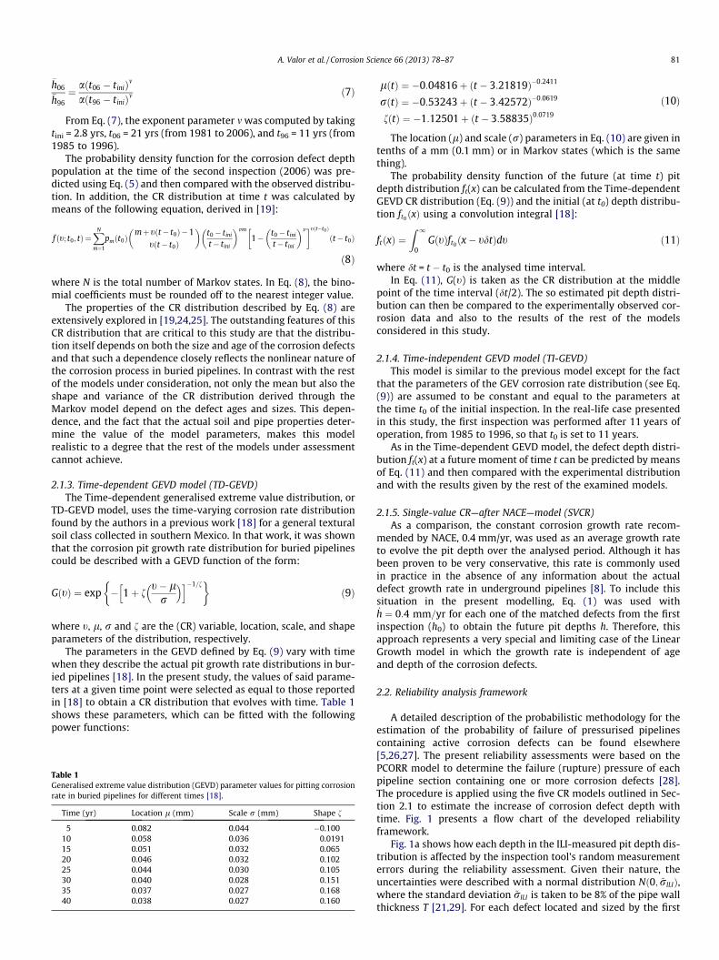
From Eq. (7), the exponent parameter m was computed by takingtini = 2.8 yrs, t06 = 21 yrs (from 1981 to 2006), and t96 = 11 yrs (from1985 to 1996).

The probability density function for the corrosion defect depthpopulation at the time of the second inspection (2006) was pre-dicted using Eq. (5) and then compared with the observed distribu-tion. In addition, the CR distribution at time t was calculated bymeans of the following equation, derived in [19]:

f ðt; t0; tÞ ¼XN

m¼1

pmðt0Þmþtðt� t0Þ�1

tðt� t0Þ

� �t0� tini

t� tini

� �vm

1� t0� tini

t� tini

� �v� �tðt�t0Þ

ðt� t0Þ

ð8Þ

where N is the total number of Markov states. In Eq. (8), the bino-mial coefficients must be rounded off to the nearest integer value.

The properties of the CR distribution described by Eq. (8) areextensively explored in [19,24,25]. The outstanding features of thisCR distribution that are critical to this study are that the distribu-tion itself depends on both the size and age of the corrosion defectsand that such a dependence closely reflects the nonlinear nature ofthe corrosion process in buried pipelines. In contrast with the restof the models under consideration, not only the mean but also theshape and variance of the CR distribution derived through theMarkov model depend on the defect ages and sizes. This depen-dence, and the fact that the actual soil and pipe properties deter-mine the value of the model parameters, makes this modelrealistic to a degree that the rest of the models under assessmentcannot achieve.

2.1.3. Time-dependent GEVD model (TD-GEVD)The Time-dependent generalised extreme value distribution, or

TD-GEVD model, uses the time-varying corrosion rate distributionfound by the authors in a previous work [18] for a general texturalsoil class collected in southern Mexico. In that work, it was shownthat the corrosion pit growth rate distribution for buried pipelinescould be described with a GEVD function of the form:

GðtÞ ¼ exp � 1þ ft� l

r

� �h i�1=f�

ð9Þ

where t, l, r and f are the (CR) variable, location, scale, and shapeparameters of the distribution, respectively.

The parameters in the GEVD defined by Eq. (9) vary with timewhen they describe the actual pit growth rate distributions in bur-ied pipelines [18]. In the present study, the values of said parame-ters at a given time point were selected as equal to those reportedin [18] to obtain a CR distribution that evolves with time. Table 1shows these parameters, which can be fitted with the followingpower functions:

Table 1Generalised extreme value distribution (GEVD) parameter values for pitting corrosionrate in buried pipelines for different times [18].

Time (yr) Location l (mm) Scale r (mm) Shape f

5 0.082 0.044 �0.10010 0.058 0.036 0.019115 0.051 0.032 0.06520 0.046 0.032 0.10225 0.044 0.030 0.10530 0.040 0.028 0.15135 0.037 0.027 0.16840 0.038 0.027 0.160

lðtÞ ¼ �0:04816þ ðt � 3:21819Þ�0:2411

rðtÞ ¼ �0:53243þ ðt � 3:42572Þ�0:0619

fðtÞ ¼ �1:12501þ ðt � 3:58835Þ0:0719

ð10Þ

The location (l) and scale (r) parameters in Eq. (10) are given intenths of a mm (0.1 mm) or in Markov states (which is the samething).

The probability density function of the future (at time t) pitdepth distribution ft(x) can be calculated from the Time-dependentGEVD CR distribution (Eq. (9)) and the initial (at t0) depth distribu-tion ft0 ðxÞ using a convolution integral [18]:

ftðxÞ ¼Z 1

0GðtÞft0ðx� tdtÞdt ð11Þ

where dt = t � t0 is the analysed time interval.In Eq. (11), G(t) is taken as the CR distribution at the middle

point of the time interval (dt/2). The so estimated pit depth distri-bution can then be compared to the experimentally observed cor-rosion data and also to the results of the rest of the modelsconsidered in this study.

2.1.4. Time-independent GEVD model (TI-GEVD)This model is similar to the previous model except for the fact

that the parameters of the GEV corrosion rate distribution (see Eq.(9)) are assumed to be constant and equal to the parameters atthe time t0 of the initial inspection. In the real-life case presentedin this study, the first inspection was performed after 11 years ofoperation, from 1985 to 1996, so that t0 is set to 11 years.

As in the Time-dependent GEVD model, the defect depth distri-bution ft(x) at a future moment of time t can be predicted by meansof Eq. (11) and then compared with the experimental distributionand with the results given by the rest of the examined models.

2.1.5. Single-value CR—after NACE—model (SVCR)As a comparison, the constant corrosion growth rate recom-

mended by NACE, 0.4 mm/yr, was used as an average growth rateto evolve the pit depth over the analysed period. Although it hasbeen proven to be very conservative, this rate is commonly usedin practice in the absence of any information about the actualdefect growth rate in underground pipelines [8]. To include thissituation in the present modelling, Eq. (1) was used with_h ¼ 0:4 mm=yr for each one of the matched defects from the firstinspection (h0) to obtain the future pit depths h. Therefore, thisapproach represents a very special and limiting case of the LinearGrowth model in which the growth rate is independent of ageand depth of the corrosion defects.

2.2. Reliability analysis framework

A detailed description of the probabilistic methodology for theestimation of the probability of failure of pressurised pipelinescontaining active corrosion defects can be found elsewhere[5,26,27]. The present reliability assessments were based on thePCORR model to determine the failure (rupture) pressure of eachpipeline section containing one or more corrosion defects [28].The procedure is applied using the five CR models outlined in Sec-tion 2.1 to estimate the increase of corrosion defect depth withtime. Fig. 1 presents a flow chart of the developed reliabilityframework.

Fig. 1a shows how each depth in the ILI-measured pit depth dis-tribution is affected by the inspection tool’s random measurementerrors during the reliability assessment. Given their nature, theuncertainties were described with a normal distribution Nð0; ~rILIÞ,where the standard deviation ~rILI is taken to be 8% of the pipe wallthickness T [21,29]. For each defect located and sized by the first

Fig. 1. Flow chart of the reliability assessment methodology: (a) Consideration of the measurement uncertainties and time evolution of a single corrosion defect depth, (b)estimation of the probability of failure (PoF) of the defect.


ILI, the resulting pit depth distribution has mean h0 and standarddeviation ~rILI . This distribution occurs at the initial time t0 and isevolved using each one of the corrosion rate models described inSection 2 to obtain the depth distribution of the defects at a futuretime t (see Fig. 1a).

Fig. 1b shows the stage that follows: the Monte Carlo frame-work. In each kth Monte Carlo step, a vector of the basic randomvariables Xi

k ¼ fhik; L

ik;D

ik; T

ik;UTSi

kg is introduced into the PCORRmodel [28] to calculate the failure pressure pi

fkassociated with

the ith defect. The statistical variables are the defect depth h andlength L at time t, the pipe diameter D, the pipe wall thickness T,and the pipe tensile strength UTS. The probabilistic distributionsof these variables are assumed to be normal and of the typeNð�x; ~rxÞ, with �x and ~rx as the mean value and standard deviationof each variable, respectively.

For each defect, the calculated failure pressure pifk

is comparedwith a value popk

taken from the operation pressure normal distri-bution Nð�pop; ~rpop

Þ. The number of failures (when popkP pi

fk) di-

vided by the total number n of Monte Carlo steps constitutes anunbiased estimator of the probability of failure PoFi of the defect[5].

For each one of the Ndef defects found in the ILI, the abovescheme is repeated n times. Therefore, the process is repeatedn � Ndef times during the assessment. This procedure is repeatedfor several future times tj with time intervals of 1 year. By theend of the computations, the probability of failure PoFi(tj) of eachone of the corrosion defects in the pipeline at each time tj has beencomputed.

To calculate the (conditional) annual probability of failurePoFann

i of the ith defect, the following expression is applied [30]:

PoFanni ðtj; tjþ1Þ ¼

PoFiðtjþ1Þ � PoFiðtjÞ1� PoFiðtjÞ

ð12Þ

where tj stands for the specific year under analysis.

Under the assumption that the corrosion defects are indepen-dent, an upper bound of the annual probability of failure of thewhole pipeline can be computed as [5,30]

PoFðtj; tjþ1Þ ¼ 1�Pi½1� PoFanni ðtj; tjþ1Þ� ð13Þ

Additionally, the pipeline’s annual failure index k at the end ofthe jth year is calculated using [1]:

kðtj; tjþ1Þ ¼PNdef

i¼1 PoFanni ðtj; tjþ1Þ

lpipeð14Þ

where lpipe is the pipeline length expressed in km. Therefore, k hasunits of failures (or incidents) per km per yr, which are commonlyexpressed as 1/(km yr).

3. Results and discussion

3.1. Performance of corrosion rate models

The five CR models outlined in Section 2 were applied to thePipe 85-1996 data set. For the five models, the analysed time spandt = t � t0 was 10 years. In the case of the Markov model, the char-acteristic pit initiation times were assumed to be tini = 2.8 yr,t0 = 11 yr, and t = 21 yr (see Eqs. (5) and (8)).

For the Time-dependent GEVD model, the CR distributions usedfor each year over the analysis interval, from the year 11 to theyear 21, were determined using Eqs. (9) and (10) and Table 1. Incontrast, for the Time-independent GEVD model, the corrosion ratedistribution used was that predicted by Eqs. (9) and (10) for the11th year.

Fig. 2a shows the initial (Pipe 85-1996) and final (Pipe 85-2006)pit depth distributions on a probability density scale of the by-ILImeasured and matched defects in the example pipeline. In this fig-ure, the defect depth is given in units of 0.1 mm or Markov states

0 20 40 60 80 100 1200.00

0.02

0.04

0.06

0.08

0.10

0.12

0.14

0.16

Den

sity

of p

roba

bilit

y

Defect depth (states)

Pipe85-1996 (bin 5) Pipe85-1996 (bin 1) Pipe85-2006 TI-GEVDl TD-GEVD Single value (NACE) Linear Growth Markov

0 1 2 3 4 50.00

0.02

0.04

0.06

0.08

0.10

Empirical CR Linear Growth TI-GEVD TD-GEVD Markov

Den

sity

of p

roba

bilit

y

Corrosion rate (states/yr)

a

b

Fig. 2. Comparison of defect depth distributions predicted by the five corrosiongrowth models under assessment.

Table 2Quality index (Eq. (15)) of the estimations made by the five CR models underassessment.

hini � hfin (states)a DLin. Growth DMarkov DTI-GEVD DTD-GEVD DSVCR

0–100 1.0290 0.6709 0.6908 0.6927 1.91063–9 1.4509 1.0534 1.3005 1.2742 2.00006–12 1.3764 0.8107 0.9273 0.8861 2.00009–15 1.3604 0.6942 0.7744 0.7567 2.000012–18 1.6757 0.8445 0.8354 0.8276 1.965515–21 1.7367 0.8863 0.9166 0.9268 1.971818–100 1.5717 0.7396 0.7465 0.7649 1.9444

a Depth intervals into which the initial (Pipe 85-1996) pit depth were catego-rised. A state is 0.1-mm wide.


(called states from here on). The initial depth distribution has beenrepresented in two ways: by a histogram comprised of five statesin each bin and by a line that goes state by state. The latter repre-sentation has been included for the sake of comparison with theSVCR (after the NACE recommendation) model, as will be seenlater. Meanwhile, the final ILI-measured depth distribution isdisplayed in the form of a histogram with five-state-wide bins.Fig. 2a also shows the estimated pit depth distributions aftera 10-yr interval as predicted by the five CR models undercomparison.

The first item of note in Fig. 2a is that the SVCR model exactlyreproduces the shape of the initial distribution, yet it is signifi-cantly shifted to the right. The estimated depth values are muchlarger than those experimentally observed or those predicted bythe rest of the models. Likewise, the Linear Growth model overes-timates the defect depth values, which in practical situationswould lead to an overestimation of the future depths in a real pipe-line and consequently to conservative maintenance schedules.

From the results shown in Fig. 2a, it can be concluded that themodels that best describe the second experimental pit depth distri-bution (Pipe 85-2006) are those that take into consideration thepipe and soil properties. However, it can be observed that theMarkov model predicts a pit depth distribution that is closer to

the experimental one than those obtained from the two GEVD-based models.

To gain a quantitative evaluation of the accuracy of the fivemodels, the relative quality index Dmodel was defined as the meansquare difference between the predicted and observed defectdepth PDFs. If f(x) is the empirical PDF and fmodel(x) is the PDF pre-dicted by the model, then Dmodel can be obtained from:

Dmodel ¼

ffiffiffiffiffiffiffiffiffiffiffiffiffiffiffiffiffiffiffiffiffiffiffiffiffiffiffiffiffiffiffiffiffiffiffiffiffiffiffiffiffiffiffiffiffiffiXN

q¼1

½f ðxqÞ � fmodelðxqÞ�2vuut ð15Þ

where q runs for all possible defect depths in both ILIs, expressed instates, which range from 1 to N.

Table 2 contains the calculated values of the quality index forthe five analysed models; the first row of this table correspondsto the entire depth distribution with Ndef = 179 defects. It can beobserved that, although the quality indexes for the GEVD-basedand Markov models are close to each other, the Markov model out-performs both of them. The Markov model not only exhibits a bet-ter quality index, it also better describes the shape of the defectdepth distribution, as seen from Fig. 2a.

For the sake of comparison, in Fig. 2b, the corrosion rate distri-butions used by each model are presented together with the corro-sion rate derived from the repeated in-line inspections. Again, theMarkov model is the one that best reproduces the empirical CRdistribution.

In an attempt to explore the characteristics of the experimentalCR derived from the comparison of the two ILIs, the corrosion ratevalues were averaged within 10-state wide depth intervals in thefirst inspection. Fig. 3 shows the corrosion rate mean and variancedependence on defect depth. In this figure, pit depths weregrouped into depth intervals of ten states; the abscissas of the rep-resented points correspond to the middle point of the interval. Thisway, each ordinate point in Fig. 3 gives the mean (or variance) ofthe corrosion rate for all defects whose depths are in the corre-sponding interval. It can be observed that both the corrosion ratemean and variance increase with defect depth, as was previouslynoted by the authors from different experimental evidence[14,19]. This result is critical to support the hypothesis of thisstudy, that a CR model should consider both the age and depthof the to-be-evolved corrosion defects together with the actualshape of the function describing the observed dependence of thecorrosion defect depth with time.

The Markov model is not only the most accurate in estimatingthe time evolution of the entire defect depth distribution, but itis also the most appropriate for estimating the time evolution ofdefect sub-populations that differ in depths, as seen from Fig. 4.To produce this figure, the defects in the initial (Pipe 85-1996)inspection were categorised into 6-state depth intervals and thedepth distribution for each interval was separately plotted as aPDF together with the depth distribution of the corresponding

5 10 15 20 25 30 35 400.0

0.4

0.8

1.2

1.6

2.0

CR mean Value

CR

mea

n (s

tate

s/yr

)

Initial defect depth (states)

0.4

0.8

1.2

1.6

2.0

CR variance

CR

var

ianc

e (s

tate

s2 /yr2 )

Fig. 3. Dependence of the empirical corrosion rate (CR) mean and variance ondefect depth in a real-life pipeline. A state corresponds to a 0.1-mm-wide depthinterval.


matched defects in the second inspection (Pipe 85-2006). Theselater depths are presented in Fig. 4 in the form of a histogram.The predicted distributions by the five models for each initialdepth subpopulation are also displayed in the same figure.

The results presented in Fig. 4 confirm that the SVCR model and,to a lesser extent, the Linear Growth model are not capable ofreproducing the observed defect depths by the time of the secondinspection. As commented earlier, the SVCR model simply shiftsthe original distribution by a fixed amount to larger depth valueswithout changing its shape. This result openly contradicts the sto-chastic nature of corrosion growth because the model cannotreproduce the inherent increase in the variance of the corrosiondepth distribution with time. This increase has been experimen-tally observed in this (Figs. 2 and 4) and previous studies (see alsoRefs. [14,17]). Therefore, the use of single-value CR distributions,no matter what growth rate value is selected to create it,2 shouldbe avoided in reliability analyses.

For its part, the Linear Growth model increasingly deviates fromthe observed depth distribution for larger initial depth values.Additionally, the predicted distributions are narrower than thoseexperimentally observed. This observation is evidence of the factthat the Linear Growth model also takes depth values from a cer-tain part of the initial distribution and only shifts them to largerdepth regions, without considering the stochastic nature of thecorrosion growth process. This behaviour differs from what isdetected experimentally; for example, Fig. 3 shows that narrowinitial depth intervals (grey lines) evolve into wider distributions(grey histograms) that cover a range of depth values broader thanthe initial one.

In marked contrast, the models that take into account the soilproperties, the GEVD-based and Markov models are capable ofreproducing the experimental results. However, in the majorityof cases (five out of six), the Markov model shows better perfor-mance than the GEVD-based models, which is quantitativelyproven in Table 2, in which the quality index Dmodel for each oneof the six cases presented in Fig. 4 is shown. In all but one case(when the initial defect depths are taken between 12 and 18states), the Markov chain model has a quality index smaller thanthose of the TI-GEVD and TD-GEVD models. For this case, the dif-ferences are �0.0091 and �0.0169, respectively. Fig. 4 and Table 2

2 The reasons behind the choice of the overly conservative corrosion rate valuerecommended by NACE to producethe single value CR distribution (SVCR) modelassessed in this study can be appraised from this result.

show that the Markov model is capable of taking into account notonly the time dependence of the corrosion rate but also its depen-dence on defect depth, as noted earlier by Caleyo et al. [19].

The reasons behind the foregoing results lie in the ability of theMarkov chain model to capture the influence of both the depth andage of the corrosion defects on the deterministic pit depth growthtogether with its ability to reproduce the stochastic nature of theprocess, also as a function of the defect’s depth and age. In compar-ing these capabilities with those shown by the rest of the models,one can draw attention to the following facts:

1. The Linear Growth model uses only the uncertainty of the ILItool to define the variance of the CR distribution to be associ-ated with each defect. Therefore, the estimated future pit depthdistribution strongly depends on the type of inspection toolused and not on the actual physical and chemical propertiesof the corrosion environment.

2. The stated disadvantage of the Linear Growth model can be fur-ther stressed by considering the hypothetical case that occurswhen the defect depth population in a pipeline is located in ahighly corrosive environment and measured by an ILI tool witha relative high accuracy and precision, e.g., inspection using anultrasound ILI tool of a highly rated gas pipeline buried in atropical clay-type soil. In such a situation, the intrinsic andrelatively high uncertainty of the corrosion process will be com-pletely lost during the estimation of future pit depths, thusleading to flawed reliability results blemished mainly byunderestimation.

3. The Time-dependent and -independent GEVD models produceresults close, yet inferior in quality, to those of the Markovchain model only because the characteristics of the soil inwhich the example pipeline is corroding were known. In theabsence of such information, when repeated ILIs were available,the Markov remains the only model that can fairly reproducethe time evolution of the corrosion defects from the depth dataof the first ILI and the value of m estimated using Eq. (7).

4. The single-value CR model fails to reproduce the stochasticnature of corrosion and its dependence on the defect depthsand ages, no matter what growth rate is used to construct it.As in the case of the Linear Growth model, its only advantageis the ease of use in pragmatic terms.

The differences in the abilities of the different models to cor-rectly describe the corrosion rate distributions and the corrosiongrowth process should markedly impact the results of the reliabil-ity estimations. The following section explores this statement infurther detail.

3.2. Probability and index of failure given by the CR models

First, the described reliability framework was applied to syn-thetic data. A hypothetical 100 km-long pipeline was used withdiameter D = 762 mm (30 in.), wall thickness T = 11.4 mm(0.45 in.), and ultimate tensile strength UTS = 455 MPa (66 ksi).These variables were considered to be normally distributed withrD = 0.254 mm (0.01 in.), rT = 1.14 mm (0.045 in.), and rUTS = 21 -MPa (3 ksi), respectively. For the sake of simplicity, the pipelinewas assumed to have only 150 defects after 20 years in operation.The calculations were carried out for a time interval from 20 to45 years (dt = 25 yrs), with a 2-yr-long time step, and the soil–pipeparameters were taken as those found for the generic (All soils) soilcategory in [16,18]. The time range was chosen to include the pipelifetimes observed in the field survey carried out by Velazquezet al., in which the soil pit growth parameters were derived fromthe soil–pipe characteristics [16]. The number of Monte Carlosimulations was set to 10,000.

0 10 20 30 40 500.0

0.1

0.2D

ensi

ty o

f pro

babi

lity


Initial depths from 3 to 9 states

0 10 20 30 40 50


Defect depth (states)0 10 20 30 40 50



0 10 20 30 40 50 600.0

0.1

0.2

Den

sity

of p

roba

bilit

y



0 10 20 30 40 50 60


Defect depth (states)0 10 20 30 40 50 60 70 80



Sing. val. (NACE)Linear GrowthMarkov

TD-GEVDTI-GEVD

1996 ILI2006 ILI

Fig. 4. Comparison of the model predictions for the defect subpopulations (by depth intervals) of the initial defect depth distribution. The estimations of each model arecompared with the experimentally observed depths in the same initial depth interval over a 10-yr period. A state corresponds to a 0.1-mm-wide depth interval.


The defect lengths were taken from a normal distribution withmean value lL = 11.4 mm (0.45 in.) and standard deviationrL = 1.14 mm (0.045 in.). This length was selected to guaranteethat rupture is the failure mode of all defects. This choice is notexpected to noticeably alter the results of the present reliabilityanalyses because they have been proven to have low sensitivityto uncertainties in defect length [5].

To investigate the behaviour of the different CR models as afunction of defect depths, log-normal distributions with differentmean (lh) and variance (r2

h) values were used to model the initialdefect depth distribution in the pipeline. Fig. 5 shows a compen-dium of the results obtained for four different initial defect depthdistributions. Fig. 5a–d correspond to depth log-normal distribu-tions with mean and standard deviation (given in mm) of (0.762,2.540), (1.778, 3.810), (3.810, 5.080), and (4.572, 7.620), respec-tively. The mean depths correspond, respectively to 6.7%, 15.5%,33% and 40% of the pipe wall thickness. It can be observed thatfor small depths (6.7% and 15.5% of the wall thickness), the LinearGrowth model underestimates the mean values of the futuredepth, which may lead to failure indices that are well below thosepredicted by the models that take into consideration the soil–pipeproperties. Meanwhile, the estimations made by the Markov modelare close to those of the TI and TD-GEVD models, especially for longintervals (longer than 15 yrs). This coincidence can be attributed tothe fact that the corrosion parameters used in these models werederived from a field survey [16] where the measured average de-fect depth was 2.02 mm (0.08 in.) and the mean pipeline age was22.9 yrs. Therefore, it is logical to expect that the models workbetter for depths and times of this order. For short time intervals,the Markov–Chain-based model estimates failure indices slightlyhigher than those given by the GEVD models. The Time-dependentGEVD model yields slightly higher failure indices than the TI-GEVDmodel, but the difference is not noteworthy.

For deeper defects (33% and 40% of the pipe wall), the LinearGrowth and Markov models produce similar annual failure indices,although the Linear Growth model produces failure index valuesthat exceed the Markov results for deeper defects and longer

exposure times, as seen from Fig. 5c and d. These indices are morethan an order of magnitude higher than those estimated by theGEVD-based models. This provides evidence that the latter modelsdo not work well when the depth values and/or the time intervalsare far from those experimentally observed in the work where theGEV distributions used in this study were obtained [18]. Therefore,as mentioned at the end of the previous section, the soil-relatedmodels are a good choice only when the pipeline under studyhas characteristics similar to those found in [16]. This first exampleshows that the Markov model remains the best option whenchoosing the CR distribution to be used in reliability analysis ofcorroding pipelines.

The next example involved the application of the described reli-ability framework to the Pipe 85-1996 data set. Fig. 6 shows theobtained failure indices for this experimental data set using thefive analysed corrosion rate distributions. In accordance with whatwas discussed above, the Single-value CR and Linear Growth mod-els overestimate the pipeline’s failure index over the analysedinterval, which means that these CR models would lead to conser-vative predictions and would recommend shortened repairintervals. For the sake of comparison, a target reliability level of10�3 per km yr has been drawn in the form of a horizontal line inthe failure index vs. time plot. For this target reliability level, theSVCR and Linear Growth models would recommend, respectively,maintenance actions 6 and 5 years before the Markov recommen-dation. As shown previously, the Markov prediction is the one thatbest describes the actual corrosion evolution (Fig. 4), such that thereliability results produced by this model can be considered closerto the true (unknown) pipeline’s reliability level.

On the other hand, the TI-GEVD and TD-GEVD models underes-timate the failure indices over the entire period analysed. However,for longer times, the differences between the predictions made bythese models and those of the Markov model become smaller, anobservation consistent with the previously noted characteristic ofthe GEVD models of being suited only for corrosion data close tothose found in [16]. The mean depth value of Pipe 85-1996 dataset is 1.70 mm (0.067 in.), compared to the mean depth value of

25 30 35 40 451E-7

1E-6

1E-5

1E-4

1E-3

0.01

0.1

1

Markov TI-GEVD Linear growth TD-GEVD Sing-val. NACE

Failu

re In

dex

t (years)

Init. depth (mm): LogN(4.572, 7.620); 150 defects

25 30 35 40 451E-7

1E-6

1E-5

1E-4

1E-3

0.01

0.1

1


Failu

re In

dex

t (years)


25 30 35 40 451E-7

1E-6

1E-5

1E-4

1E-3

0.01

0.1

1


Failu

re In

dex

t (years)


25 30 35 40 451E-7

1E-6

1E-5

1E-4

1E-3

0.01

0.1

1


Failu

re In

dex

t (years)


a

c

b

d

Fig. 5. Failure index evolution as predicted by the five models under assessment for several defect depth distributions, with mean values representing: (a) 6.7%, (b) 15.5%, (c)33%, and (d) 40% of the pipe wall thickness in a hypothetical 100 km-long pipeline.

14 16 18 20 22 24 26 28 301E-7

1E-6

1E-5

1E-4

1E-3

0.01

0.1

1


Failu

re In

dex

t (years)

Pipe85-199611 - 30 years

Fig. 6. Time evolution of the failure index in the Pipe 85-1996 ILI as predicted bythe five models under assessment.


2.02 mm (0.079 in.) found in [16]. Taking this into account, to-gether with the fact that the pipe age (11 yrs) is substantially lessthan the average pipeline age (22.9 yrs) found in [16], one canexplain the inability of the GEVD models under assessment to

correctly predict the failure index for this pipeline over the analysisinterval (Fig. 6). With the passage of time, the defect depths be-come larger and the uncertainty due to the stochastic nature ofcorrosion increases, as shown in Fig. 4. This explains why the GEVDresults approach the Markov results for longer exposure times.

4. Conclusions

Corrosion defect depth and reliability estimations have beenperformed using different corrosion rate distributions derived fromvarious corrosion growth models for underground pipelines. It hasbeen demonstrated that during reliability analysis it is crucial tocorrectly select the defect growth model to make accurate predic-tions of the time evolution of corrosion defects and of the probabil-ity of failure of these defects.

It has been shown that single value CR distributions should notbe used when performing reliability analysis. Using a single corro-sion rate value yields a result that is very different from whathappens in reality: the corrosion rate actually responds to adistribution of values that varies over time in mean, variance,and shape, given the stochastic nature of corrosion. These changes(consideration of which is critical to any reliability analysis) are notreproduced by single value CR distributions.

For its part, the Linear Growth model underestimates or overes-timates the corrosion depth growth depending on the initial defect


depths and the period for corrosion activation. For the real pipelineanalysed in this work, the Linear Growth model overestimates thecorrosion rate with respect to the empirical values determined bythe comparison of repeated ILIs. This, in turn, leads to an overesti-mation of the failure rates of the pipeline under study. However, ithas been shown that the Linear Growth model can underestimatethe corrosion growth for shallow defects while it gives similar orslightly higher results (for failure indices or probabilities offailures) than the Markov model for deep defects (>30% of the pipewall thickness) and long exposure times (>20 yrs).

The GEVD-based corrosion models (Time-independent and -dependant) are a good choice for describing the defect depthevolution with time, provided that the mean depth values and pipeage are consistent with those found in the investigation by Velaz-quez et al. [16] in which the model parameters were derived. Ingeneral, the Time-dependent model works better than the Time-independent model. However, when the actual experimentalconditions deviate from those found in the field survey by Velaz-quez et al. [16], the GEVD models become useless.

The Markov model has been proven as the model of choice forcorrect prediction of the corrosion defect depth evolution andpipeline reliability. This model works well over a wide range ofpipe ages and defect depths. The model based on the outlined Mar-kov chain methodology is capable of correctly predicting not onlythe time evolution of the entire defect depth population but alsothe evolution of the defects in subpopulations within differentdepth intervals; it is also the only model that reproduces the timeevolution of the corrosion defects from the depth data of the firstILI and the value of m estimated from two (or more) repeated ILIs.This result means that no physical or chemical information is re-quired to assess the actual corrosivity of the soil and its influenceon the corrosion process to make relatively accurate estimationsof the pipeline reliability over time. Finally, it is the only modelcapable of capturing the intrinsic (unavoidable) stochastic natureof the corrosion process independent of the inspection toolmeasurement errors or the initial defect depth distribution in thepipeline.

References

[1] M. Stephens, M. Nessim, A comprehensive approach to corrosion managementbased on structural reliability methods, in: Proceedings of IPC2006, 6thInternational Pipeline Conference, September 2006, Calgary, Alberta, Canada,Paper no. IPC2006-10458.

[2] H.A. Kishawy, H.A. Gabbar, Review of pipeline integrity management practices,Int. J. Press. Vessels Pip. 87 (2010) 373–380.

[3] F. Caleyo, L. Alfonso, J.M. Hallen, On the estimation of failure rates of multiplepipeline systems, ASME, J. Press. Vessel Technol. 30 (2008) 1–8.

[4] I.S. Cole, D. Marney, The science of pipe corrosion: a review of the literature onthe corrosion of ferrous metals in soils, Corros. Sci. 56 (2012) 5–16.

[5] F. Caleyo, J.L. González, J.M. Hallen, A study on the reliability assessmentmethodology for pipelines with active corrosion defects, Int. J. Press. VesselsPip. 79 (2002) 77–86.

[6] S.X. Li, S.R. Yu, H.L. Zeng, J.H. Li, R. Liang, Predicting corrosion remaining life ofunderground pipelines with a mechanically-based probabilistic model, J.Petrol. Sci. Eng. 65 (2009) 162–166.

[7] T. Zimmerman, M. Nessim, M. McLamb, B. Rothwell, J. Zhou, A. Glover, Targetreliability levels for onshore gas pipelines, in: Proceedings of the 4thInternational Pipeline Conference IPC’02, Calgary, Canada, 2002, PaperIPC2002-27213.

[8] J.M. Race, S.J. Dawson, L.M. Stanley, S. Kariyawasam, Development of apredictive model for pipeline external corrosion rates, J. Pipeline Eng. 6 (1)(2007) 15–29.

[9] Mazura Mat Din, Norhazilan Md. Noor, Md. Asri Ngadi, Khadijah Abd. Razak,Maheyzah Md. Siraj, Automated matching systems and correctional methodfor improved inspection data quality, Int. J. Comput. Theory Eng. 3 (2) (2011)248–254.

[10] Standard Recommended Practice RP 0169–92: Control of External Corrosionon Underground or Submerged Metallic Piping Systems, NACE 1992.

[11] Standard Recommended Practice TG041: Pipeline External Corrosion DirectAssessment Methodology, NACE 2002.

[12] A.K. Sheikh, J.K. Boah, D.A. Hansen, Statistical modeling of pitting corrosionand pipeline reliability, Corrosion 46 (3) (1990) 190–197.

[13] Z. Szklarska-Smialowska, Pitting Corrosion of Metals, National Association ofCorrosion Engineers, Houston, 1986.

[14] D. Rivas, F. Caleyo, A. Valor, J.M. Hallen, Extreme value analysis applied topitting corrosion experiments in low carbon steel: comparison of blockmaxima and peak over threshold approaches, Corros. Sci. 50 (2008) 3193–3204.

[15] D.D. Macdonald, Critical Issues in Understanding Corrosion andElectrochemical Phenomena in Super Critical Aqueous Media, Paper No.04484, CORROSION ’04, New Orleans, LA, March 2004.

[16] J.C. Velazquez, F. Caleyo, A. Valor, J.M. Hallen, Predictive model for pittingcorrosion in buried oil and gas pipelines, Corrosion 65 (2009) 332–342.

[17] P.M. Aziz, Application of the statistical theory of extreme values to the analysisof maximum pit depth data for aluminum, Corrosion 13 (1956) 495–506.

[18] F. Caleyo, J.C. Velázquez, A. Valor, J.M. Hallen, Probability distribution of pittingcorrosion depth and rate in underground pipelines: a Monte Carlo study,Corros. Sci. 51 (2009) 1925–1934.

[19] F. Caleyo, J.C. Velázquez, A. Valor, J.M. Hallen, Markov chain modelling ofpitting corrosion in underground pipelines, Corros. Sci. 51 (2009) 2197–2207.

[20] Specification for Line Pipe, API Specification 5L, 42nd ed., January 2000,American Petroleum Institute, Washington D.C., 1999.

[21] F. Caleyo, L. Alfonso, J.H. Espina-Hernández, J.M. Hallen, Criteria forperformance assessment and calibration of in-line inspections of oil and gaspipelines, Meas. Sci. Technol. 18 (7) (2007) 1787–1799.

[22] B. Rajani, Y. Kleiner, Comprehensive review of structural deterioration of watermains: physically based models, Urban Water 3 (3) (2001) 151–164.

[23] E. Parzen, Stochastic Processes, Classics in Applied Mathematics, Society forIndustrial and Applied Mathematics (SIAM), PA, 1999.

[24] J.C. Velázquez, A. Valor, F. Caleyo, V. Venegas, J.H. Espina-Hernandez, J.M.Hallen, M.R. Lopez, Study helps model buried pipeline pitting corrosion, OilGas J. 107 (27) (2009) 64–73.

[25] J.C. Velázquez, A. Valor, F. Caleyo, V. Venegas, J.H. Espina-Hernandez, J.M.Hallen, M.R. Lopez, Corrosion – conclusion: pitting corrosion models improveintegrity management, reliability, Oil Gas J. 107 (28) (2009) 56–62.

[26] F. Caleyo, J. Hallen, J.L. Gonzalez, F. Fernandez, Pipeline inspection – 1:Reliability based assessment method assesses corroding pipelines, Oil Gas J.101 (1) (2003) 54–58.

[27] F. Caleyo, J. Hallen, J.L. Gonzalez, F. Fernandez, Pipeline inspection –Conclusion: reliability-based assessment method assesses corrodingpipelines, Oil Gas J. 101 (2) (2003) 56–61.

[28] N. Leis, D.R. Stephens, An alternative approach to assess the integrity ofcorroded line pipe – Part I: Current status and Part II: Alternative criterion, in:Proceedings of the Seventh International Offshore and Polar EngineeringConference, Honolulu, USA, May 25–30, 1997, pp. 624–641.

[29] M. Beller, K. Reber, Tools, vendors, and services: a review of current in-lineinspection technologies, in: J. Tiratsoo (Ed.), Pipeline Pigging & IntegrityTechnology, third ed., Scientific Surveys Ltd, Beaconsfield, UK and ClarionTechnical Publishers, Houston, TX, 2003, pp. 357–374.

[30] G. Pognonec, V. Gaschignard, P. Notariani, Predictive assessment of externalcorrosion on transmission pipelines, in: Proceedings of the 7th InternationalPipeline Conference IPC2008, Calgary Canada, September 29–October 2, 2008,Paper No. IPC2006-64316.

Reliability assessment of buried pipelines based on different corrosion rate models

Documents

Transcript of Reliability assessment of buried pipelines based on different corrosion rate models