Regulatory dynamics on random networks: asymptotic periodicity and modularity

arX

iv:0

707.

1551

v3 [

mat

h.D

S] 1

Feb

200

8

REGULATORY DYNAMICS ON RANDOM NETWORKS:

ASYMPTOTIC PERIODICITY AND MODULARITY

A. CROS, A. MORANTE, AND E. UGALDE

CUCEI, Universidad de Guadalajara, 44430 Guadalajara, Mexico,

F. Ciencias, Universidad Autonoma de San Luis Potosı, 78000 San Luis Potosı, Mexico, &

I. Fısica, Universidad Autonoma de San Luis Potosı, 78000 San Luis Potosı, Mexico.

Abstract. We study the dynamics of discrete–time regulatory networks on randomdigraphs. For this we define ensembles of deterministic orbits of random regulatorynetworks, and introduce some statistical indicators related to the long–term dynamics ofthe system. We prove that, in a random regulatory network, initial conditions convergealmost surely to a periodic attractor. We study the subnetworks, which we call modules,where the periodic asymptotic oscillations are concentrated. We proof that those modulesare dynamically equivalent to independent regulatory networks.

Keywords: regulatory networks, random graphs, coupled map networks.

1. Introduction

Numerous natural and artificial systems can be though as a collection of basic units in-teracting according to simple rules. Examples of this interacting systems are the ge-netic regulatory networks, composed of interactions between DNA, RNA, proteins, andsmall molecules. In social or ecological networks, a similar regulatory dynamics mayalso be considered. The traditional way to model these systems is by using coupleddifferential equations, and more particularly systems of piecewise affine differential equa-tions (see [6, 9, 17]). Finite state models, better known as logical networks, are also used(see [11, 13, 19]). Within these modeling strategies, the interacting units have a regularbehavior when taken separately, but are capable to generate global complex dynamicswhen arranged in a complex interaction architecture. In all the models considered so far,each interacting unit regulates some other units in the collection by enhancing or repress-ing their activity. It is possible then to define an underlying network with interactingunits as vertices, and their interactions as arrows connecting those vertices. The theo-retical problem we face here is to understand the relation between the structure of theunderlying network, and the possible dynamical behaviors of the system. We will do thisin the context of a particular class of models first introduced in [22], and further studied

1

http://arXiv.org/abs/0707.1551v3

2 A. CROS, A. MORANTE, AND E. UGALDE

in [5] and [16]. In these models, the level of activity of each unit is codified by a positivereal number. The system evolves synchronously at discrete time steps, each unit followingan affine contraction dictated by the activity level and interaction mode of its neighboringunits. The contraction coefficient of those transformations determines the degradationrate at which, in absence of interactions, the activity of a given unit vanishes. In theframework of this modeling we have proved general results concerning the constrains im-posed by the structure of the underlying network, over the possible asymptotic behaviorsof a fixed system [16]. In the present paper, following [22], we will focus on the asymptoticdynamics of regulatory systems whose interactions are chosen at random at the beginningof the evolution. Within this approach, individual orbits are elements of a sample space,and the statistical indicators we will study become orbit dependent random variables. Theprobability measures we used are built from a fixed probability distribution over the setof possible underlying networks. Then, given a fixed underlying network, we associate asign to each one of its arrows, depending on whether the interaction they represent areactivations or inhibitions. Positive and negative signs are randomly chosen, keeping afixed proportion of negative arrows inside a given statistical ensemble of systems. In thisway it is possible to study certain characteristics of the asymptotic dynamics, as functionof the degradation rate and the proportion of inhibitory interactions.

Our first result states that in a random regulatory network, initial conditions convergealmost surely to a periodic attractor. This result points to the conclusion that in regulatorydynamics, the origin of the complexity is the coexistence of multiple dynamically simpleattractors. We prove that this is the case in a full measure set in the parameter space.

According to our preliminary numerical explorations, the long–term oscillations of thesystem concentrate on subnetwork whose structure depends on the parameters of thestatistical ensemble of regulatory networks. Our second result states that the dynamics onecan observe when restricted to the oscillatory subnetwork, is equivalent to the dynamicssupported by the subnetwork considered as an isolated system. This result allows usto introduce the concept of modularity. If we call module any observable oscillatorysubnetwork, then, according to our result, the dynamics of a small network is preservedwhen it appears as a module in a larger network. We interpret this as the emergence ofmodularity. This result allows us to predict admissible asymptotic behaviors in regulatorynetworks admitting disconnected oscillatory subnetworks. It is worth mentioning thatthis kind of modularity was already studied in the context of Boolean networks [3] andmore recently, in continuous–time regulatory networks [10]. Our approach allows a formalapproach to the problems addressed in those works.

The paper is organized as follows. In the next section we will introduce the objects understudy, then in Section 3 we will state the results, and present some of the proofs. Afterreviewing two examples, which we do in Section 4, we will give the proofs of the twomore technical results in Section 5. The paper ends with a section of final comments andconclusions.

This work was supported by CONACyT through the grant SEP–2003–C02–42765, and bythe cooperation ECOS–CONACyT–ANUIES M04–M01. E. U. thanks Bastien Fernandezfor his suggestions and comments.

REGULATORY DYNAMICS ON RANDOM NETWORKS 3

2. Preliminaries

2.1. Regulatory Networks as Dynamical Systems.

The interaction architecture of the regulatory network is encoded in a directed graphG = (V,A), where vertices V represent interacting units, and the arrows A ⊂ V ×V denoteinteraction between them. To each interaction (u, v) ∈ A we associate a threshold T(u,v) ∈[0, 1], and a sign σ(u,v) ∈ −1, 1 that is chosen according to whether this interaction is aninhibition or an activation. We quantify the activity of each unit v ∈ V with real numberxv ∈ [0, 1]. Thus, the activation state of the network at a given time t is determined bythe vector xt ∈ [0, 1]V . The influence of a unit u over a target unit v turns on or off,depending on its sign, when the value of xu trespasses the threshold T(u,v). The evolution

of the network is generated by the iteration of the map FG,σ,T,a : [0, 1]V → [0, 1]V suchthat

(1) xt+1 = FG,σ,T,a(xt) := axt + (1 − a)DG,σ,T (xt),

where the contraction rate a ∈ [0, 1) determines the speed of degradation of the activityof the units in absence of interaction, and the interaction term DG,σ,T : [0, 1]V → [0, 1]V isthe piecewise constant function defined by

(2) DG,σ,T (x)v :=1

Id(v)

∑

u∈V :(u,v)∈A

H(σ(u,v)

(

xu − T(u,v)))

.

Here H : R → R is the Heaviside function, and Id(v) := #u ∈ V : (u, v) ∈ A standsfor the input degree of the vertex v. We will be referring to the discontinuity set of thetransformation DG,σ,T , which is

(3) ∆T :=

x ∈ [0, 1]V : xu = Tu,v for some(u, v) ∈ A

.

For each a ∈ [0, 1), the transformation FG,σ,T,a is a piecewise affine contraction withdiscontinuity set ∆T .

From now on, by a discrete–time regulatory network we will mean a discrete–time dy-namical system ([0, 1]V , FG,σ,T,a), with phase space [0, 1]V , and evolution generated by

the piecewise affine contraction FG,σ,T,a : [0, 1]V → [0, 1]V defined in Equation (1). Thediscrete–time regulatory networks studied here have interactions of equal strength, andthey act additively on each target unit. More general discrete–time regulatory networkshave been considered in [5, 16].

2.2. Statistical Ensembles.

We build our statistical ensembles as follows. We fix the value of the contraction ratea ∈ [0, 1) and the set V representing the interacting units. Then we consider the set of allpossible piecewise transformations,

(4) Fa,V :=

FG,σ,T,a : G := (V,A), σ ∈ −1, 1A, T ∈ [0, 1]A

.

The individual elements of our statistical ensembles are couples (FG,σ,T,a,x), with FG,σ,T,a ∈Fa,V and x ∈ [0, 1]V . A couple (FG,σ,T,a,x) determines a deterministic orbit xt :=F tG,σ,T,a(x)∞t=0.


We supply the sample space Fa,V × [0, 1]V with a probability measure as follows. First wefix a probability distribution PG over the set GV := (V,A) : A ⊂ V × V of all directedgraphs with vertex set V . Then, for η ∈ [0, 1] and G = (V,A), we choose sign −1 withprobability η and +1 with probability 1 − η, independently for each arrow in G. Thethresholds are independent and uniformly distributed random variables in [0, 1]A, as wellas the initial conditions in [0, 1]V . In this way we obtain the probability measure Pa,η onFa,V × [0, 1]V such that

(5) Pa,η (FG,σ,T,a,x) : T ∈ I,x ∈ J = PG(G) × PA,η(σ) × vol(I) × vol(J ),

for all rectangles I ⊂ [0, 1]A and J ⊂ [0, 1]V . Here PA,η : −1, 1A → [0, 1] is such that

(6) PA,η(σ) =∏

(u,v)∈A

(

σ(u,v) + 1

2− σ(u,v)η

)

,

and vol stands for the Lebesgue measure on the corresponding euclidean spaces.

2.3. Some graph–theoretical notations and definitions.

A path in G = (A,V ) is a sequence u0, u1, . . . , uk, with ui ∈ V and (ui, ui+1) ∈ A for eachi. The length of a path is the number of arrows it contains. A cycle is a path u0, u1, . . . , uk,where u0 = uk. We say that the vertices u, v ∈ V are connected if there exists a cycleu0, u1, . . . , uk such that u, v ∈ u0, u1, . . . , uk. The connected components of G are themaximal subgraphs of G such that all their vertices are connected. The distance betweentwo vertices u, v ∈ V , which we denote dG(u, v), is the length of the shortest directedpath whose end vertices are u and v.

2.4. The oscillatory subnetwork and the asymptotic period.

To each couple (FG,σ,T,a,x) we associate a directed graph Gosc := (Vosc, Aosc) ⊆ G, theoscillatory subnetwork, defined by

Aosc := (u, v) ∈ A : H(xtu − Tu,v) does not converge,

Vosc := v ∈ V : ∃ u ∈ V such that (u, v), (v, u) ∩ Aosc 6= ∅.

By definition, the oscillatory subnetwork is spanned by all the arrows whose activationstate H(σu,v(xu − Tu,v)) changes infinitely often. This subnetwork is the equivalent,in discrete–time regulatory networks, to the dynamical islands introduced in [10] forcontinuous–time regulatory networks. They are also related to the clusters of relevantelements in Boolean networks, as they were defined in [3]. Unlike the differential equa-tions and the finite state modeling strategies of regulatory dynamics [14, 20, 21], ourmodels admit oscillations in all network topologies, regardless the distribution of activa-tions and inhibitions through the graph. This is possible because of the discreteness oftime, and continuity of the state variable. Therefore, oscillatory subnetworks may occurin any discrete–time regulatory network.

The oscillatory subnetwork can be seen as a random variable

Gosc : Fa,V × [0, 1]V → G⊆V := (V , A) : V ⊂ V and A ⊂ V × V ,


from which we can derive other statistical indicators, as for instance its size #Vosc, thenumber nc(Gosc) of its connected components, and its the degree distribution

pGosc(k) :=#v ∈ Vosc : Idosc(v) = k

#Vosc,

where Idosc(v) := u ∈ Vosc : (u, v) ∈ Aosc.

Another statistical indicator we will consider is the asymptotic period of a given orbit.Denote by Perτ (FG,σ,T,a) the set of all FG,σ,T,a–periodic points of minimal period τ , i. e.,

(7) Perτ (FG,σ,T,a) =

x ∈ [0, 1]V : F τG,σ,T,a(x) = x and F t

G,σ,T,a(x) 6= x if t < τ

.

We will say that the asymptotic FG,σ,T,a–period of x ∈ [0, 1]V is τ if there exists y ∈Perτ (FG,σ,T,a), such that

limt→∞

|F tG,σ,T,a(x) − F t

G,σ,T,a(y)| = 0.

We will denote this by P (FG,σ,T,a,x) = τ .

3. Results

3.1. The asymptotic period.

To each finite set V , and a ∈ [0, 1), we associate the sample space Fa,V × [0, 1]V , with Fa,V

as in Equation (4). We supply this sample space with the product sigma–algebra, takingfor [0, 1]V and [0, 1]A, the corresponding Borel sigma–algebras. The next result concernsthe asymptotic period (FG,σ,T,a,x) 7→ P (FG,σ,T,a,x).

Theorem 1. Given a finite set V , and a ∈ [0, 1), the function P : Fa,V × [0, 1]V → N

which assigns to (FG,σ,T,a,x) ∈ Fa,V × [0, 1]V the value of the asymptotic FG,σ,T,a–periodof x, is a measurable function. Furthermore, for each η ∈ [0, 1],

Pa,η

(FG,σ,T,a,x) ∈ Fa,V × [0, 1]V : P (FG,σ,T,a,x) < ∞

= 1.

This expected but nontrivial result says that a random orbit will almost certainly approacha periodic orbit, otherwise said, an initial condition almost certainly converges to a periodicattractor. It is because of this result that we can restrict ourselves to the study of periodicorbits, even though the parameter set for which the orbits are infinite may be uncountable(see [5]). We could therefore redefine the oscillatory subnetwork by saying that, after atransitory, their arrows change periodically their activation state. The proof of this resultand some related comments are left to Subsection 5.1.


3.2. Modularity.

In this paragraph we will consider probability measures obtained by conditioning on asubnetwork, from a given statistical ensemble of regulatory networks. Given Pa,η on Fa,V ×[0, 1]V , and a subnetwork G := (V , A) ∈ G⊆V , we define the analogous probability measure

Pa,η,G on Fa,V × [0, 1]V , such that

(8) Pa,η,G

(FG,σ,T ,a,y) : T ∈ I, y ∈ J

:=

PA,η(σ) vol(I) vol(J ) if G = G,0 otherwise,

for each σ ∈ −1, 1A, and all rectangles I ⊂ [0, 1]A and J ⊂ [0, 1]V . As before, voldenotes the corresponding Lebesgue measures. This measure can also be seen as themarginal of Pa,V obtained by projecting over V ⊂ V , then conditioned to have underlyingnetwork G ∈ GV .

Theorem 2. Fix a ∈ [0, 1), η ∈ [0, 1], and a digraph G = (V , A) ∈ G⊆V with V ( V . If thedigraph distribution PG is such that PG(G) > 0 for all G ∈ GV , and if Pa,η(Gosc = G) > 0,then we can associated to G:

a) a digraph extension Gext := (V,A) ∈ GV ,

b) rectangles I := I × I ′ ⊂ [0, 1]A × [0, 1]A\A and J := J × J ′ ⊂ [0, 1]V × [0, 1]V \V ,

c) and for each σ ∈ −1, 1A, an extension σext ∈ −1, 1A such that σext|A = σ.

These associated objects satisfy

Gosc(FGext ,σext,T,a,x) ⊆ G ∀ T ∈ I, x ∈ J , and σ ∈ −1, 1A.

Furthermore, Gext, I, and J , define surjective transformations

d) ΦA : I × I ′ → [0, 1]A, such that ΦA(T × T ′) = DAT + CA with DA diagonal andCA constant,

e) and similarly, ΦV : J × J ′ → [0, 1]V such that ΦV (x × x′) = DV x + CV , with DV

diagonal and CV constant.

These transformations satisfy

ΦV FG,σ,T,a(x) = FG,σ,ΦA(T ),a ΦV (x),

for all T ∈ I, and x ∈ J .

The proof of this result follows from a construction, and it is postponed to Section 5. Letus from now expose its interpretation and some of its consequences. We can divide thisTheorem into two parts, the first part concerns the stability of the oscillatory subnetworks.It says that if an oscillatory subnetwork G := (V , A) has positive probability to occur,

then to each signs matrix σ ∈ −1, 1A it corresponds an oscillatory subnetwork whichis subgraph of G. Furthermore, the set of initial conditions and thresholds for which agiven subgraph of G is the oscillatory subnetwork, is a rectangle with nonempty interior.Therefore, each of those subgraphs is stable under small changes in the thresholds T ∈[0, 1]A, and in the initial condition x ∈ [0, 1]V . The size of the maximal perturbationdepends on the position of (T,x) with respect to the borders of the above mentionedrectangle.


More interestingly, the second part of the theorem states that if an oscillatory subnetworkhas positive probability to occur, then the dynamics one can observe when restricted tothat subnetwork is equivalent to the dynamics supported by the subnetwork considered asan isolated system. The equivalence is achieved through the transformation ΦA and ΦV . Itis because of this equivalence that we can talk about modularity. Indeed, if we call moduleany oscillatory subnetwork occurring with positive probability, then this theorem can berephrased by saying that each orbit admissible in a module considered as an isolatedsystem, can be achieved, up to a change of variables, as the restriction of an orbit inthe original system. The network extension Gext, the values of the external thresholdsI ′ ∈ [0, 1]A\A, and the external initial conditions J ′ ∈ [0, 1]V \V , can be though as theanalogous in our systems, to the functionality context defined in [18] for logical networks.Using their nomenclature, our theorem ensures that if an oscillatory subnetwork has apositive probability to occur, then there is positive measure set of contexts making thissubnetwork functional.

An interesting consequence of the previous theorem is the following.

Corollary 1. Fix a ∈ [0, 1), η ∈ [0, 1], and G ≡ G1 ∪ G2 ∈ G⊆V , with G1 := (V1, A1) andG2 := (V2, A2) vertex disjoint and such that V1 ∪ V2 ( V . If the digraph distribution PG issuch that PG(G) > 0 for all G ∈ GV , and if Pa,η(Gosc ⊆ G) > 0, then

Pa,η(P = τ) > C∑

lcm(τ1,τ2)=τ

Pa,η,G1(P = τ1) Pa,η,G2(P = τ2),

with C > 0 a constant depending on Pa,η and G.

The probabilities in the sum at right hand side of the inequality are analogous probabilitymeasures of the kind defined by Equation (8). They are obtained as marginal probabilitycorresponding to projections over vertex the sets V1 and V2, then conditioned to haveunderlying network G1 and G2 respectively.

In [3] the authors study the relationship between the modular structure and the periodsdistribution in Boolean networks. The previous corollary establishes such a relation inthe framework of discrete–time regulatory networks. Our result relates the distribution ofthe asymptotic period of a network G, to the distribution of the asymptotic period of itsoscillatory subnetworks considered as isolated systems. It establishes in particular thatthe observable asymptotic periods of G are the least common multiples of the observableasymptotic periods of its oscillatory subnetworks.

Proof. First notice that, for each G ∈ G⊆V we have

Pa,η(P = τ) > Pa,η(P = τ |Gosc ⊆ G) × Pa,η(Gosc ⊆ G).

Let G = (V , A) = (V1 ∪ V2, A1 ∪ A2), with G1 := (V1, A1) and G2 := (V2, A2) vertexdisjoint. Theorem 2 ensures the existence of the following objects associate to G: a) theextension of G, a digraph Gext := (V,A) ∈ GV such that G ⊆ Gext, b) two affine surjectivetransformations

ΦA : I → [0, 1]A1 × [0, 1]A2 and ΦV : J → [0, 1]V1 × [0, 1]V2 ,


and c) for each σ ≡ σ(1) × σ(2) ∈ −1, 1A1 ×−1, 1A2 , an extension σext ∈ −1, 1A suchthat σ|A1∪A2 = σ. From the second part of the theorem it follows that

(9) ΦV

(

F tGext,σext,T,a(x)

)

= F tG1,σ(1),T (1),a

(

y(1))

× F tG2,σ(2),T (2),a

(

y(2))

,

for all t ∈ N and (T,x) ∈ I×J . Here we have used ΦV (T ) ≡ T (1)×T (2) ∈ [0, 1]A1 ×[0, 1]A2

and ΦV (x) ≡ y(1) × y(2) ∈ [0, 1]V1 × [0, 1]V2 . For i = 1, 2, and each σ(i) ∈ −1, 1Ai andτi ∈ N, let us define

PGi,σ(i),τi:=(

T (i),y(i))

∈ [0, 1]Ai × [0, 1]Vi : P(

FGi,σ(i),T (i),a,y(i))

= τi

.

Defining Φ : I × J → [0, 1]A × [0, 1]V such that Φ(T,x) := ΦA(T ) × ΦV (x), it followsfrom (9) that

Pa,η

(

P = τ |Gosc ⊆ G)

>PG(Gext)

Pa,η(Gosc ⊆ G)

∑

σ=σ(1)×σ(2)

PA,η(σext)

×∑

lcm(τ1,τ2)=τ

vol Φ−1(

PG1,σ(1),τ1× PG2,σ(2),τ2

)

,

where vol denotes Lebesgue measure in [0, 1]A × [0, 1]V . Let us now use the decomposition

I = I × I ′ ⊂ [0, 1]A × [0, 1]A\A and J = J × J ′ ⊂ [0, 1]V × [0, 1]V \V . According toTheorem 2, we have

Φ((T × T ′) × (x × x′)) = D(T × x) + C

where D is a diagonal linear bijection, and C is a constant. With this,

Pa,η

(

P = τ |Gosc = G)

>PG(Gext) vol(I ′ × J ′)

|D| Pa,η(Gosc ⊆ G)

∑

σ=σ(1)×σ(2)

PA,η(σext)

×∑

lcm(τ1,τ2)=τ

vol1

(

PG1,σ(1),τ1

)

× vol2

(

PG2,σ(2),τ2

)

,

where vol denotes the Lebesgue measure in [0, 1]A\A × [0, 1]V \V , voli denotes the Lebesguemeasure in [0, 1]Ai × [0, 1]Vi for i = 1, 2, and |D| denotes the determinant of the transfor-mation D. From here, and taking into account the definition in Equation (8), we have

Pa,η

(

P = τ |Gosc = G)

>PG(Gext) vol(I ′ × J ′)min(η, 1 − η)#(A\A)


×∑

σ=σ(1)×σ(2)

PA1,η

(

σ(1))

× PA2,η

(

σ(2))

×∑

lcm(τ1,τ2)=τ

vol1

(

PG1,σ(1),τ1

)

× vol2

(

PG2,σ(2),τ2

)

>PG(Gext) vol(I ′ × J ′) min(η, 1 − η)#(A\A)


×∑

lcm(τ1,τ2)=τ

Pa,η,G1(P = τ1) Pa,η,G2(P = τ2),


and the result follows with C := PG(Gext) × vol(I ′ × J ′) × min(η, 1 − η)#(A\A)/|D|.

3.3. Sign Symmetry.

The next result illustrates how a structural constrain in the underlying random networkmanifests in the distribution of the statistical indicators. Here, the fact that the underlyingrandom digraph does not admit cycles of odd length, implies a symmetry on the statisticalindicators with respect to the change of sign in the interactions. Let us remind that foreach η ∈ [0, 1] and a ∈ [0, 1), the probability measure Pa,η on Fa,V × [0, 1]V which definesa statistical ensemble, is obtained from a fixed distribution PG over the finite set of alldirected graphs with vertices in V . We have the following.

Proposition 1. If the distribution PG over the set GV of all directed graphs with verticesin V is such that PGG ∈ GV : G admits a cycle of odd length = 0, then

Pa,η (P = τ) = Pa,1−η (P = τ) , ∀τ ∈ N,

Pa,η

(

Gosc = G)

= Pa,1−η

(

Gosc = G)

∀ G ∈ G⊆V ,

for each η ∈ [0, 1].

Statistical ensembles of regulatory networks whose underlying digraphs are random trees(as defined in Subsection 4.1 below) clearly satisfy the hypothesis of Proposition 1. Ran-dom subnetworks of the square lattice also have this property. Therefore, for regulatorydynamics over those kind of digraphs, the statistical indicators we consider are left invari-ant under the symmetry η 7→ 1 − η.

In the proof of Proposition 1, we will need the following.

Lemma 1. For each G := (V,A) ∈ GV , and σ ∈ −1, 1V we have,

vol

(T,x) ∈ [0, 1]A × [0, 1]V :

F tG,σ,T,a(x) : t ∈ N

∩ ∆T = ∅

= 1.

where ∆T :=

x ∈ [0, 1]V : xu = Tu,v for some(u, v) ∈ A

is the discontinuity set of thepiecewise constant part of FG,σ,T,a.

This lemma directly follows from the arguments developed below, in paragraphs 5.1.3and 5.1.4, inside the proof of Theorem 1.

Proof of Proposition 1. First notice that, for each G = (A,V ) ∈ GV and σ ∈ −1, 1A wehave

PA,1−η(−σ) =∏

(u,v)∈A

(

−σ(u,v) + 1

2+ σ(u,v)(1 − η)

)

=∏

(u,v)∈A

(

σ(u,v) + 1

2− σ(u,v)η

)

= PA,η(σ).

Let us suppose that all the cycles in G have even length, and for each connected componentof G := (A, V ) ⊆ G = (A,V ) ∈ GV , choose a pivot vertex u ∈ V . With this define


ΨA : [0, 1]A → [0, 1]A and ΨV : [0, 1]V → [0, 1]V such that

ΨA(T )(u,v) :=

1 − T(u,v) if dG(u, u) ∈ 2N

T(u,v) otherwiseΨV (x)u :=

1 − xu if dG(u, u) ∈ 2N

xu otherwise,

for each u, v ∈ V . Here dG denotes vertex distance induced by the digraph G, as defined inSubsection 2.3. Both ΨA and ΨV are affine isometries, therefore they preserve the Lebesguemeasure in [0, 1]A and [0, 1]V respectively. If dG(v, u) is even, then ΨV (x)v = 1 − xv, andfor each u such that (u, v) ∈ A, ΨV (x)u = xu and ΨA(T )(u,v) = T(u,v). In this case wehave

FG,−σ,ΨA(T ),a(ΨV (x))v = a(1 − xv) +1 − a

Id(v)

∑

u∈V :(u,v)∈A

H(

−σ(u,v)

(

xu − T(u,v)

))

= a(1 − xv) +1 − a

Id(v)

∑

u∈V :(u,v)∈A

(

1 − H(

σ(u,v)

(

xu − T(u,v)

)))

= 1 − FG,σ,T,a(x)v = ΨV (FG,σ,T,a(x))v ,

for each x 6∈ ∆T . On the other hand, if dG(v, vpivot) is odd, we have ΨV (x)v = xv, and foreach u such that (u, v) ∈ A, ΨV (x)u = 1 − xu and ΨA(T )(u,v) = 1 − T(u,v). In this case

FG,−σ,ΨA(T ),a(ΨV (x))v = axv +1 − a

Id(v)

∑

u∈V :(u,v)∈A

H(

−σ(u,v)

(

(1 − xu) −(

1 − T(u,v)

)))

= axv +1 − a

Id(v)

∑

u∈V :(u,v)∈A

H(

σ(u,v)

(

xu − T(u,v)

))

= FG,σ,T,a(x)v = ΨV (FG,σ,T,a(x))v ,

for each x 6∈ ∆T . Taking into account Lemma 1, F tG,−σ,ΨA(T ),a(ΨV (x)) = ΨV (F t

G,σ,T,a(x))

for all t ∈ N, for almost all (x, T ) ∈ [0, 1]A × [0, 1]V . Since ΦV is an isometry, we immedi-ately have

vol

(T,x) ∈ [0, 1]A × [0, 1]A : P (FG,−σ,ΨA(T ),a,ΨV (x)) = P (FG,σ,T,a,x)

= 1,

for all G := (V,A) ∈ GV with no odd cycles, and every σ ∈ −1, 1A. Since both ΨA andΨV preserve the respective Lebesgue measure, and PG(G admits an odd cycle) = 0, weobtain

Pa,η(P = τ) =∑

G∈GV

PG(G)∑

σ∈−1,1A

PA,1−η(−σ)

×vol

(T,x) : P (FG,−σ,ΨA(T ),a,ΨV (x)) = τ

=∑

G∈GV

PG(G)∑

σ∈−1,1A

PA,1−η(−σ) vol (T,x) : P (FG,−σ,T,a,x) = τ

= Pa,1−η(P = τ),

for all τ ∈ N, and this concludes the proof of the first claim in the proposition.


For the second claim, if F tG,σ,T,a(x) /∈ ∆T , then

H(

σ(u,v)(FtG,σ,T,a(x)u − T(u,v))

)

= H(

−σu,v

(

ΨV (F tG,σ,T,a(x))u − ΨA(T )(u,v)

))

= H(

−σu,v

(

F tG,−σ,ΨA(T ),a(ΨV (x))u − ΨA(T )(u,v)

))

.

Therefore, by Lemma 1,

vol

(T,x) ∈ [0, 1]A × [0, 1]A : Gosc(FG,−σ,ΨA(T ),a,ΨV (x)) = Gosc(FG,σ,T,a,x)

= 1,

for all G := (V,A) ∈ GV all of whose cycles have even length, and every σ ∈ −1, 1A.From here, taking into account that PG(G admits an odd cycle) = 0, and the fact thatthat ΨA and ΨV preserve the Lebesgue measure, we obtain

Pa,η(Gosc = G) =∑

G∈GV

PG(G)∑

σ∈−1,1A

PA,1−η(−σ)

×vol

(T,x) : Gosc(FG,−σ,ΨA(T ),a,ΨV (x)) = G

=∑

G∈GV

PG(G)∑

σ∈−1,1A

PA,1−η(−σ) vol

(T,x) : Gosc(FG,−σ,T,a,x) = G

= Pa,1−η(Gosc = G),

for all G ∈ G⊆V , and the proof is completed.

4. Examples

In this section we present, as a matter of illustration, two families of random digraphswhich we have explored numerically. A detailed numerical study, which requires massivecalculations, is out of the purpose of the present work, and is left for a future research.Instead, in this section we make some general observations suggested by a preliminarynumerical exploration of these examples.

4.1. Two Families of Random digraphs.

We consider two kind of distributions PG on the set GV := (V,A) : A ⊂ V × V of alldirected graph with vertex set V . On one hand we have a directed version of the classicalErdos–Renyi ensemble, which we define as follows.

Fix a vertex set V and p ∈ (0, 1), and consider the probability distribution Pp : GV → [0, 1]

such that Pp(A) = p#A. According to this, a directed graph contains the arrow (u, v)with probability p, and the inclusion of different vertices are independent and identicallydistributed random variables. The typical Erdos–Renyi graph is statistically homogeneous,thus suited for a mean field treatment. Most of the rigorous results concerning randomgraphs refer to these kind of models (see [4, 8] and references therein).

The other family of random digraphs we will refer to derives from the famous Barabasi–Albert model of scale–free random graphs, whose popularity relies on the ubiquity of thescale–free property [2, 15]. A dynamical construction of scale–free graphs was proposed


by Barabasi and Albert in [1] (see [8] for a more rigorous presentation). Their modelincorporates two key ingredients: continuous growth and preferential attachment. Weimplemented their construction as follows. For n = 0, we take G0 = Km0 , the completesimple undirected graph in m0 vertices. Then, for each n > 1, a new vertex vn+1 is addedto the graph Gn := (En, Vn). This new vertex form new edges with randomly chosenvertices in Vn. The probability for v ∈ Vn to be chosen is proportional to its degree in G0,i. e,

vn+1, v ∈ En with probability pn(v) :=#u ∈ Vn : u, v ∈ En

#En.

At the (n + 1)–th step we obtain a graph Gn+1 with an increased vertex set Vn+1 :=Vn ∪ vn+1 and an enlarged edge set En+1. This random iteration continues until apredetermined number N of vertices is obtained. In this scheme we are able to add morethan one edge at each iteration. If on the contrary, we allow only one new edge at eachtime step, and we start with m0 = 2 vertices choosing at the 1–th step one of the twopreexisting vertices to form a new edge with with probability 1/2, then the resulting graphwould be a random scale–free tree [8]. In any case, the final graph GN−m0 is turned into adirected graph G = (V,A) by randomly assigning a direction to each edge u, v ∈ EN−m0 .In our case we choose one of the two possible directions with probability 1/4, and giveprobability 1/2 to the choice of both directions. This procedure generates a probabilitydistribution PBA in GV := (V,A) : A ⊂ V × V .

4.2. Erdos–Renyi.

We generated random digraphs of the Erdos–Renyi kind with 100 vertices, and probabilityof connection p ∈ 0.2, 0.4, 0.6, 0.8. For p fixed and each η ∈ 0, 0.1, 0.2, . . . , 1, webuild 20 graphs, to which we randomly and uniformly assign thresholds, and signs withprobability PA,η. By taking a ∈ 0.0, 0.1, 0.2, . . . , 0.8, we obtain 7920 regulatory networks,20 for each triplet (p, a, η) ∈ 0.2, 0.4, 0.6, 0.8 × 0.0, 0.1, . . . , 0.8 × 0, 0.1, 0.2, . . . , 1.Finally, for each one of those dynamical systems we run 30 initial conditions randomlytaken from [0, 1]100, and we let the system evolve in order to determine the correspondingoscillatory subnetwork and the asymptotic period.

The characteristics of the oscillatory subnetwork depend strongly on the parameter a, andless noticeably on η. We have observed that the mean size of the oscillatory subnetworkdecreases with a in a seemingly monotonous way, and does not appear to depend on η.The mean number of connected components never exceeded 2. A crude inspection of thedegree distributions of the oscillatory subnetworks suggests that they form an ensembleof the Erdos–Renyi type, nevertheless, any conclusion in this direction requires a moredetailed numerical study. Finally, the mean value of the asymptotic period seems to growwith both a and η. It increases monotonously with a, while for each fixed a, it reaches alocal maximum around η = 0.5.

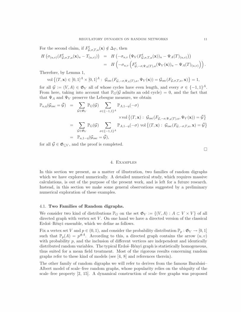
As a matter of illustration, in Figure 1 we show two digraph with vertex set V =1, 2, . . . , 50. At the left side we draw a random digraph G ∈ GV according to thedistribution Pp, with p = 0.1. The signs of the arrows correspond to a random choiceaccording to PA,η, with η = 0.5, i. e., both signs have the same probability to be chosen.The digraph at right is the oscillatory subnetwork G = Gosc(FG,σ,T,a,x), corresponding to


a certain choice of thresholds T ∈ [0, 1]A and initial condition x ∈ [0, 1]V . The contrac-tion rate was a = 0.2. In the oscillatory subnetwork, the direction of an arrow (u, v) isindicated by marking head v with a × sign.

-30

-20

-10

0

10

20

30

-30 -20 -10 0 10 20 30

-30

-20

-10

0

10

20

30

-40 -30 -20 -10 0 10 20 30

Figure 1. An Erdos–Renyi network and corresponding oscillatory sub-network. The underlying graph was built with a connection probabilityp = 0.1, and the oscillatory subnetwork corresponds to a random initialcondition, with random threshold values, and contraction rate a = 0.2.Signs are codified by colors: blue for +1, and red for -1. They appear withequal probability η = 0.5. In the oscillatory subnetwork, the direction ofan arrow is indicated by marking its head vertex with a ×.

4.3. Barabasi–Albert.

Following the procedure described in 4.1 we generate, starting from a complete graphin m0 = 5 vertices, ensembles of random digraphs of the Barabasi–Albert kind of sizeN = 100. For each η ∈ 0, 0.1, 0.2, . . . , 1, we generate 20 random graphs, then we turnthem into directed graphs by choosing one of the two possible directions with probability1/4, and both directions with probability 1/2. Finally we randomly assign thresholds,and signs with probability PA,η, to each one of the 20 resulting digraphs. By ranginga ∈ 0.0, 0.2, 0.4, 0.6, we obtain 880 regulatory networks, 20 for each couple (a, η) ∈0.0, 0.2, 0.4, 0.6 × 0, 0.1, 0.2, . . . , 1. Then, for each one of those dynamical systems,we randomly select 30 initial conditions in [0, 1]100, and let the system evolve in order todetermine the corresponding oscillatory subnetwork and the asymptotic period.

For this family of random networks, the mean size of the oscillatory subnetwork behavesin a similar way as for the Erdos-Renyi family, i. e., it increases nonmonotonously with η,with a local maximum at η = 0.5, and decreases monotonously with a. The mean numberof connected components (ranging from 0 to 10) shows a similar behavior with respect toboth η and a, with a very noticeable increase around η = 0.5. On the other hand, thedistribution of the asymptotic period becomes broader as we approach η = 0.5, and foreach value of η, the mean value of the asymptotic period grows with a. It is worth tonotice that these distributions become broader as a increases, and at the same time the


number of connected components grows. This behavior is consistent with the proliferationof periods predicted by Corollary 1, in the case of a statistical ensemble whose oscillatorysubnetworks have many connected components.

In Figure 2 we show two digraph with vertex set V = 1, 2, . . . , 50. At the left side wedraw a random digraph G ∈ GV according to the distribution PBA. The sign of the arrowsis randomly chosen by using the distribution PA,η with η = 0.5, i. e., both signs have thesame probability. The digraph at right is the oscillatory subnetwork G = Gosc(FG,σ,T,a,x),

determined by a random choice of thresholds T ∈ [0, 1]A and initial condition x ∈ [0, 1]V ,with contraction rate a = 0.2. In the oscillatory subnetwork, the direction of the arrowsis indicated by marking the head with a ×.

-20

-10

0

10

20

30

-30 -20 -10 0 10 20 30

-30

-20

-10

0

10

20

30

40

-30 -20 -10 0 10 20 30

Figure 2. A Barabasi–Albert network and corresponding oscillatory sub-network. The underlying graph was built according to the procedure de-scribed in Paragraph 4.1, starting with m0 = 3 vertices. The oscillatorysubnetwork corresponds to a random initial condition, with random thresh-old values, and contraction rate a = 0.2. Signs are codified by colors: bluefor +1, and red for -1. They appear with equal probability η = 0.5. In theoscillatory subnetwork, the direction of the arrows is indicated by markingthe head with a ×.

In Figure 3 we show the behavior of the probability to approach a fixed point, and theprobability for the asymptotic period to be equals 2, both as a function of a and η. Thispicture summarizes the statistics of the 26400 orbits generated on Barabasi–Albert likenetworks, and presents the symmetry η → 1−η predicted by Proposition 1. This symmetryis expected in an ensemble of regulatory network whose underlying digraphs have no oddlength cycles. Though the underlying networks of the experiments we performed haveboth odd and even length cycles, there is a larger proportion of even lengths amongst thecycles of small length.

5. Proofs


.............................................

........................................................

.........................................................

.............................

........

.......................................

...............................................................................

...............................................................................

...........................................

........

..............................................................................

...............................................................................

...............................................................................

....

..........

..........

.................................................................................................................................................

..........

..........

..................................................................................................................................................

..........

..........

.................................................................................................................................................

..........

..........

.................................................................................................................................................

..........

.............................................................................

..........

............................................................................

..........

..........................................................................

..........

...........................................................................

..........

............................................................................

..........

...........................................................................

..........

........................................................................... hhhh

hhh

hhhhhhhh

hhhhhhhh

h!!!!!

!!!!!!!!!!...

.......

..................

........................

...............

.................................

,,,,

.................................

"""

.

.

.

.

.

.

.

.

.

.

.

.

.

.

.

.

###

.........................

.....

.........

........

........

........

........

...

.....

....

....

..........

................

........

....

....

..

.......

................

....

....

.................

.................

..........

...

.....

.........

................

.................

.

.

.

.

.

.

.

.

.

.

.

.

.

.

.

.

.

.

.

.

.

.

.

.

.

.

.

.

.

.

.

.

.

.

.

.

.

.

.

.

..

..............

.

.

.

.

........

"""

....

.............

...

.....

####

...........

....

....

.........................

.........

....

....

..

........

.........

.........

........

...

.....

..

.......

........

..

.......

..

.......

........

.........

................

""""

.

.

.

.

.

.

.

.

.

.

.

.

.

.

.

.

.

.

.

.

.

""""

..................

.

.........

""""

.........

..........

........

""""

.

.

.

.

.

.

.

.

.

.

.

.

.

.

.

.

.

.

.

.

.

.

.

.

.

.

.

.

.

.

.

.

.

.

.

.

.

.

.

.

.

.

.

.

.

.

.

.

.

.

.

.

.

........

..

.......

...

.............

..............

....

.............

..........

...

.............

.........

..

.......

....

....

........

..........

.........

...................

........

.

.

.

.

.

.

.

.

.

.

.

.

.

.

.

.

.

.

.

.

.

.

.

.

.

.

.

.

.

.

.

.

.

.

.

.

.

.

.

.

.

.

.

.

.

........

..........

.........

..

.......

..

..

.......

.

.

.

.

.

.

.

.

.

.

.

.

.

""""

"""" ..

.......

.

.........

"""" ..

.......

.................

....

....

..................

...

.....

....

............

!!!!

........

..

.......

...

.....

!!!!

........

!!!!

..

.......

...

.....

.

.

.

.

.

.

.

.

.

.

.

.

.

.

.

.

.

.

.

.

.

.

.

.

.

.

.

.

.

.

.

.

.

.

.

.

.

.

.

.

.

.

.

.

.

.

.

.

.

.

.

.

.

.

.

.

.

.

.

.

.

.

.

.

.

.

.

.

..

.......

.

.........

...

....."

"""

.

.

.

.

.

.

.

.

.

.

.

.

.

.

.

.

.

.

.

........

.........

..

.......

..........

.........

.

.

.

.

.

.

.

.

.

.

.

.

..........

..

.......

0.80.60.40.2

a

0.6

0.4

0.2

0η 10.90.80.70.60.50.40.30.20.10

Pa,η(P = 1)

..............................................................................

...............................

..........................................

...................................................................

.....

........

.......................................................................................

............................................................................

.............................................................................

........

................................................

............................................................................

...............................................................................

.....................................

..........

..........

.................................................................................................................................................

..........

..........

..................................................................................................................................................

..........

..........

.................................................................................................................................................

..........

..........

.................................................................................................................................................

..........

..........

.................................................................................................................................................

..........

..........................................................................................

..........

...........................................................................

..........

............................................................................

..........

..............................................................................

..........

..............................................................................

..........

............................................................................ hhhh

hhhh

hhhhhhhh

hhhhhhhh

h!!!!!!

!!!!!!!!!!

.

.

.

.

.

.

.

.

.

.

.

.

.

.

.

.

.

.

.

.

.

.

.

.

.

.

.

.

.

.

.

.

.

.

.

.

.

.

.

.

.

.

.

.

.

.

.

.

.

.

.

.

.

.

.

.

.

.

.

.

.

.

.

.

.

.

...............................................

hhhh

..................................

.

.

.

.

.

.

.

.

.

.

.........

.................

.

.

.

.

.

.

.

.

.

.

.

.

.

.

.

.

.

.

.

.

.

.

.

.

.

.

.

.

.

.

.

.

.

.

.

.

.

.

.

.

.

.

.

......................

............

.

.

.

.

.

.

.

.

.

.

.

.

.........................

.........

..........

........

!!!!

.........

........

....................

........

!!

.

.

.

.

.

.

.

.

.

.

.

.

.

.

.

.

.

.

.

.

.

.

.

.

.

.

.

.

.

.

.

.

.

.

.

.

.

.

.

.

.

.

.

.

.

.

.

.

.

.

.

.

.

.

.

.

.

.

.

.

.

.

.

.

.

.

.

!!!.........

.

.

.

.

.

.

.

.

.

.

.

.........

........

!!!

.

.

.

.

.

.

.

.

.

.

.

.

.

.

.

.

.

.

.

.........

.........

!!!

.........

!!!! ..

...

.........

.

.

.

.

.

.

.

.

.

.

.

.

.........

..........

!!!!

........

........

.

.........

..

.......

!!!!

........

!!!!

.........

!!!!

.........

!!!!

........

!!!!

PPPP

........

!!!!

!!!!

hhhh

........

!!!!

((((............

!!!! ..

...............

!!!!

........

!!!!

........

!!!!

!!!! ..

...............

!!!!

........

!!!!

!!!!

..........

...........

!!!! ..

...............

!!!!

.

.

.

.

.

.

.

.

.

.

.

.

.

.

.

.

.

.

.

.

.

.

.

.

.

.

.

.

.

.

.

.

.

.

.

.

.

.

.

.

.

.

.

.

.

........

!!!!!!!!...

......

!!!! ..

.......

.......

!!!! ..

................

!!!!

................

.

.

.

.

.

.

.

.

.

.

.

.

.

.

........

!!!!..........

..

.......

.........................!!!!!!!

!!!

!!!!

........

!!!!

!!!! ..

..............

!!!!

!!!!

!!!! ....

....

!!!! ..

....... ........

!!!!

........

!!!!

...............

!!!!

.................

!!!! ..

......................

........

!!!!

!!!! ....

....

....................

.........!! .................

!!!!!!

!!!

.........

..........

!!!! ..

......

............................ ...........

.....

!!!!

.......................

........

!!!! ..

..................

```

!!!! ..

......

.........

....................

.........

!!!! ...

.....

..................

........

..

.............

.

.

.

.

.

.

.

.

.

.

.

.

.

.

.

.

.

.

.

.

........

.

.........

..........

........

...........

.........

.

................

.........

...............

............

.......

.........

..............

..................

.......

...........................

...............

!!............

!!!.............

!!!

.......

!!!..

.............

!!!!

........

!!!!

.........

!!!!

!!!! ...

.....

!!!!

........

!!!!

.................

!!!!

!!!! ..

..............

!!!!

........

!!!!

!!!! ..

......

!!!! ..

.......

!!!! ...

.....

!!!!

!!!!

!!!! ..

.......

...

.....

...

.............0.8

0.60.40.2

a

0.6

0.4

0.2

0η 10.90.80.70.60.50.40.30.20.10

Pa,η(P = 2)

Figure 3. At the top, the probability to approach a fixed point in theBarabasi–Albert ensembles, as a function of a and η. At the bottom, theprobability for the asymptotic period to be equals 2, also as a function ofa and η, for the same ensembles.

5.1. Proof of Theorem 1.

Given G = (V,A), we will use the distance dmax(x,y) := maxi |xi −yi| in both [0, 1]V and[0, 1]A. As usual, dmax(x, E) := infdmax(x,y) : y ∈ E for x ∈ [0, 1]F and E ⊂ [0, 1]F .First notice that for G, σ and a fixed, the set

(10) OG,σ,a :=

(T,x) ∈ [0, 1]A × [0, 1]V : inft>0

dmax

(

F tG,σ,T,a(x),∆T

)

> 0

is open. Indeed, if (T,x) ∈ OG,σ,a, then dmax

(

F tG,σ,T,a(x),∆T

)

> 3ε, for some ε > 0 and

all t > 0. The orbit does not change if we perturb T , i. e., for each T ′ ∈ Bε(T ) we have


F tG,σ,T ′,a(x) = F t

G,σ,T,a(x) for all t ∈ N. Furthermore, since dmax

(

F tG,σ,T ′,a(x),∆T ′

)

> 2ε,

then dmax

(

F tG,σ,T ′,a(y),∆T ′

)

> ε for all y ∈ Bε(x), therefore Bε(T ) × Bε(x) ⊂ OG,σ,a.

Since for each G, σ and a fixed, the set OG,σ,a is open in [0, 1]A × [0, 1]V , then

(11) Oa,V :=⋃

G

⋃

σ∈−1,1A

⋃

(FG,σ,T,a,x) : (T,x) ∈ OG,σ,a

is measurable in Fa,V × [0, 1]V .

5.1.1. The asymptotic period is measurable in Oa,V .

Fix G, σ and a, and take (T,x) ∈ OG,σ,a such that P (FG,σ,T,a,x) = τ . There existsy ∈ Perτ (FG,σ,T,a) and N ∈ N, such that

dmax

(

FNG,σ,T,a(x), y

)

< ε :=inft>0 dmax

(

F tG,σ,T,a(x),∆T

)

3.

Hence, for each t > 0 we have dmax

(

FN+tG,σ,T,a(x), F t

G,σ,T,a(y))

< atε. By the same argument

as in the previous paragraph, dmax

(

FN+tG,σ,T ′,a(y), F t

G,σ,T ′,a(y))

< atε+ aN+tε < 2atε for all

t > 0. Therefore P (FG,σ,T ′,a,y) = τ for all (T ′,y) ∈ Bε(T ) × Bε(x). In this way we haveproved that for each G, σ and a fixed, the set

O(τ)G,σ,a :=

(T,x) ∈ [0, 1]A × [0, 1]V : P (FG,σ,T,a,x) = τ

is an open set in [0, 1]A × [0, 1]V , therefore

P−1τ ∩ Oa,V :=⋃

G

⋃

σ∈−1,1A

⋃

(FG,σ,T,a,x) : (T,x) ∈ O(τ)G,σ,a

is measurable in Fa,V × [0, 1]V .

5.1.2. The asymptotic period is finite in Oa,V .

For (FG,σ,T,a,x) ∈ Oa,V let x ∈ closure(

F tG,σ,T,a(x) : t ∈ Nt∈N

)

be such that

inft>0

dmax

(

F tG,σ,T,a(x),∆T

)

= dmax (x,∆T ) = ε > 0.

Notice that (FG,σ,T,a, x) ∈ Oa,V too, and inft>0 dmax

(

F tG,σ,T,a(x),∆T

)

= dmax (x,∆T ) = ε.

For N ∈ N such that dmax

(

FNG,σ,T,a(x), x

)

< ε we have dmax

(

FN+tG,σ,T,a(x), F t(x)

)

6 atε

for all t > 0. Now, for τ ∈ N such that aτ < 1/4 and dmax

(

FN+τG,σ,T,a(x), x

)

< ε/4, we have

dmax

(

F τG,σ,T,a(x), x

)

6 dmax

(

FN+τG,σ,T,a(x), x

)

+ dmax

(

FN+τG,σ,T,a(x), F τ (x)

)

< ε/4 + aτε < ε/2.


Since inft>0 dmax

(

F tG,σ,T,a(x),∆T

)

= ε, then

dmax

(

F kτG,σ,T,a(x), F

(k−1)τG,σ,T,a (x)

)

<a(k−1)τε

2<

ε

22k−1,

for all k ∈ N. Hence y := limk→∞ F kτG,σ,T,a(x) exists and satisfies F τ

G,σ,T,a(y) = y. Further-

more, since dmax (x, y) < ε∑∞

k=1 21−2k = 2ε/3, then

dmax

(

FN+kτG,σ,T,a(x), y

)

6 dmax

(

FN+kτG,σ,T,a(x), F kτ

G,σ,T,a(x))

+ dmax

(

F kτG,σ,T,a(x), y

)

<5akε

3,

for each k ∈ N, which implies limt→∞

∣

∣

∣F tG,σ,T,a(x) − F t

G,σ,T,a(y)∣

∣

∣= 0, where y = Fn

G,σ,T,a(y)

with n ≡ −N mod τ . It follows from here that P (FG,σ,a,T ,x) = τ . In addition, since

y ∈ closure(

F tG,σ,T,a(x) : t ∈ Nt∈N

)

, then min06t<τ dmax

(

F tG,σ,a,T (y),∆T

)

= ε.

5.1.3. The complement of Oa,V has zero measure for a < maxu∈V (Id(u) + 1)−1.

Fix G, σ, a, and for (T,x) /∈ OG,σ,a let D(t) := DG,σ,a(FtG,σ,T,a(x)) for each t ∈ N. Then,

there exists a sequence tk ∈ Nk∈N, and u, v ∈ V , such that

T(u,v) = limk→∞

(

atkxu + (1 − a)

tk∑

t=1

at−1D(tk−t)u

)

= (1 − a) limk→∞

(

tk∑

t=1

at−1D(tk−t)u

)

.(12)

For each x ∈ [0, 1]V fixed, define the fiber

(13) CG,σ,a(x) :=

T ∈ [0, 1]A : (T,x) /∈ OG,σ,a

.

Then, according to Equation (12) we have

CG,σ,a(x) ⊂⋃

(u,v)∈A

T ∈ [0, 1]A : T(u,v) ∈1 − a

Id(u)× closure (ΩG,a,u)

,

where

ΩG,a,u :=

∞⋃

N=1

N−1∑

s=0

asks : (ks)N−1s=0 ∈ 0, 1, . . . , Id(u)N

.

If a < (Id(u) + 1)−1 for some u ∈ V , then closure (ΩG,a,u) is a Cantor set of dimensionlog(Id(u) + 1)/ log(1/a) < 1. Hence, Fubini’s Theorem implies, for a < maxv∈V (Id(u) +1)−1, that the fiber CG,σ,a(x) has zero #A–dimensional volume for each x ∈ [0, 1]V .


5.1.4. The complement of Oa,V has zero measure for a > maxu∈V (Id(u) + 1)−1.

The fact that vol (CG,σ,a(x)) = 0 for each x ∈ [0, 1]A and arbitrary a ∈ (0, 1), derives

from a result by Kruglikov and Rypdal. Theorem 2 in [12] gives an upper bound forthe topological entropy of the symbolic system associated to a non–degenerated piecewiseaffine map. The upper bound is related to the exponential rate of angular expansion underthe action of the map. For piecewise affine conformal maps, which is the case of discrete–time regulatory networks, this upper bound vanishes. Hence, Kruglikov and Rypdal’stheorem directly applies to our case, implying that

(14) lim supN→∞

log #L(N)(T,x,u)

N= 0,

where for each G, σ, and a fixed,

L(N)(T,x,u) :=

(kt+s)N−1s=0 ∈ 0, 1, . . . , Id(u)N : DG,σ,T (F t

G,σ,T,a(x))u =kt

Id(u)∀t ∈ N

.

Therefore, for each T , there exists N = N(T,x, u) ∈ N such that #L(N)(T,x,u) 6 ((1+a)/2a)N .

Fix u ∈ V , and for each N ∈ N and D ⊂ 0, 1, . . . , Id(u)N , define

TD :=

x =

∞∑

t=0

atkt : (k(k+1)N−1, . . . ,kkN ) ∈ D ∀k > 0

.

With this we have, for the fiber CG,σ,a(x) defined in (13), the inclusion(15)

CG,σ,a(x) ⊂⋃

(u,v)∈A

⋃

N∈N

⋃

D⊂0,1,...,Id(u)N

#D6((1+a)/2a)N

T ∈ [0, 1]A : T(u,v) ∈1 − a

Id(u)× closure(TD)

.

Now, for each m ∈ N, a prefix k ∈(

L(N)(T,x,u)

)mdefines an interval

Ik :=

x =∞∑

t=0

ωtat : (ωt)

mN−1t=0 = (kmN−t)

mNt=1

,

and we have

closure(TD) =

∞⋂

m=1

(

⋃

k∈Dm

closure (Ik)

)

.

Since vol(Ik) = vol(closure(Ik)) = Id(u)amN/(1 − a) for each k ∈(

L(N)(T,x,u)

)m, then

vol(closure(TD)) 6 (#D)mamN Id(u)

1 − a,

for each m ∈ N. Hence, vol(closure(TD)) = 0 for each D ⊂ 0, 1, . . . , Id(u)N such that#D 6 ((1 + a)/2a)N . Taking into account (15), Fubini’s Theorem implies, that the fiberCG,σ,a(x) has zero #A–dimensional volume for each x ∈ [0, 1]V .


Using once again Fubini’s, we finally conclude,

Pa,η(Fa,V × [0, 1]V \ Oa,V ) 6∑

G∈GV

∑

σ∈−1,1A

PG(G)PA,ησ

∫

x∈[0,1]Vvol (CG,σ,a(x)) dx = 0.

Remark 1. In the statement of Theorem 1 we can replace the probability measure Pa,η

by any other Borel measure P in Fa,V × [0, 1]V such that, for each G ∈ GV , σ ∈ −1, 1A,

and x ∈ [0, 1]V fixed, the #A–dimensional projection

PT (J ) := P(FG,σ,T,a,x) ∈ Fa,V × [0, 1]V : T ∈ J

is absolutely continuous with respect to the Lebesgue measure.

Remark 2. From the arguments developed in Paragraph 5.1.3, it follows that for a <minu∈V (Id(u) + 1)−1, the set OG,σ,a defined in (10) is open and dense. This ensures thatorbits are generically uniformly far from the discontinuity set. As a consequence, periodicattractors not intersecting the discontinuity set are generic for a < minu∈V (Id(u) + 1)−1.On the other hand, the argument in Paragraph 5.1.4 ensures, as long as we considerdistributions absolutely continuous with respect to Lebesgue for thresholds, that orbits arealmost surely uniformly far from the discontinuity set. Hence, in the general case, almostall initial conditions converge to periodic attractors not intersecting the discontinuity set.

5.2. Proof of Theorem 2.

This theorem consist of two claims. The first one establishes the stability of the oscillatorysubnetworks, while the second one gives the equivalence between the dynamics restricted tothat subnetwork and the dynamics supported by the subnetwork considered as an isolatedsystem. Both claims follow from direct computations.

5.2.1. Stability of the oscillatory subnetworks.

Since Pa,η(Gosc = G) > 0, then, there exists G ∈ GV , σ ∈ −1, 1A, and (T , x) ∈ OG,σ,a,such that Gosc(FG,σ,T ,a, x) = G. As proved in Paragraph 5.1.2, there exists 0 < ε < 1/2,

τ ∈ N, and y ∈ Perτ (FG,σ,T ,a), such that limt→∞

∣

∣

∣F tG,σ,T ,a

(x) − F tG,σ,T ,a

(y)∣

∣

∣ = 0 and

inft>0

dmax

(

F tG,σ,T ,a

(x),∆T

)

= min06t<τ

dmax

(

F tG,σ,T ,a

(y),∆T

)

= 2ε.

From this it readily follows that Gosc(FG,σ,T,a,y) = G for each (T,y) ∈ Bε(T ) × Bε(y).

Let us now extend G, σ, and T , and redefine y at each vertex v ∈ V such that Idosc(v) =Id(v) (remind that Idosc(v) := #u ∈ V : (u, v) ∈ A ≡ Aosc). Choose u /∈ V , and include

the arrow (u, v) in A. Then, if yu < 1−2ε, define σ(u,v) = 1 and T(u,v) = 1−ε. Otherwise,

if yu > 2ε, make σ(u,v) = −1 and T(u,v) = ε. Finally, redefine yv = Id(v) yv/(Id(v) + 1) +1/(Id(v) + 1) at that vertex. A simple computation shows that, in the redefined system,

Gosc(FG,σ,T,a,y) = G, for each (T,y) ∈ Bε(T )×Bε(y). Therefore, taking into account that


by hypothesis PG(G) > 0 for all G ∈ GV , we can assume without lost of generality thatIdosc(v) < Id(v) for all v ∈ V .

By definition, if (u, v) ∈ A \ A then θ(u,v) := H(σ(u,v)(ytu − T(u,v))) remains constant in

time, as well as D(v) :=∑

(v,u)∈A\A θ(v,u) for each v ∈ V . Let us now modify σ and

T for the arrows leaving G. For u ∈ V , and each v /∈ V , if D(u) > 0, make T(u,v) 7→

T(u,v) × D(u)/Id(u), and

σ(u,v) 7→

σ(u,v) if θ(u,v) + σ(u,v) ∈ −1, 2−σ(u,v) if θ(u,v) + σ(u,v) ∈ 0, 1.

Otherwise, if D(u) = 0, then T(u,v) 7→ T(u,v) × (Id(u) − Idosc(u))/Id(u) + Idosc(u)/Id(u),and

σ(u,v) 7→

−σ(u,v) if θ(u,v) + σ(u,v) ∈ −1, 2σ(u,v) if θ(u,v) + σ(u,v) ∈ 0, 1.

This modification in σ and T uncouples the dynamics on V from that on V \V , so that now

we can set σ|A ≡ σ for arbitrary σ ∈ −1, 1A. In this way we obtain a digraph extension

Gext := G ⊃ G, and for each σ ∈ −1, 1A an extension σext := σ ∈ −1, 1A with σext|A =σ. For any of this extensions, a direct computation shows that limt→∞ F t

Gext,σext,T,a(x)v =

D(v)/Id(v) = yv for v /∈ V , and F tGext,σext,T,a

(x)v ∈ [D(v)/Id(v), (D(v) + Idosc(v))/Id(v)],

for all t > 0 and v ∈ V , whenever

x ∈ J × J ′ :=

∏

v/∈V

[yv − ε, y + ε] ∩ [0, 1]

×

∏

v∈V

[

D(v)

Id(v),D(v) + Idosc(v)

Id(v)

]

,

and

T ∈ I×I ′ :=

∏

(u,v)∈A\A

[T(u,v) − ε, T(u,v) + ε] ∩ [0, 1]

×

∏

(u,v)∈A

[

D(u)

Id(u),D(u) + Idosc(u)

Id(u)

]

.

Therefore, Gosc(FGext,σext,T,a,x) ⊆ G for each (T,x) ∈ I × J :=(

I × I ′)

×(

J × J ′)

, and

σ ∈ −1, 1A.

5.2.2. Equivalence to the subnetwork considered as an isolated system.

We will use the same notation as in Subsubsection 5.2.1. Let σ := σext, and each (T,x) ∈(

I × I ′)

×(

J × J ′)

, and t ∈ N, let xt := F tGext,σext,T,a

(x). For each v ∈ V , the term

D(v) :=∑

(u,v)∈A\A

H(

σ(u,v)

(

xtu − T(u,v)

))

=∑

(u,v)∈A\A

H(

σ(u,v)

(

F tG,σ,T ,a

(y)u − T(u,v)

))

,

remains constant in time. Since σ|A ≡ σ,

xt+1v = axt

v +Idosc(v)

Id(v)

(1 − a)

Idosc(v)

∑

(u,v)∈A

H(σ(u,v)(xtu − T(u,v)))

+ (1 − a)D(v)

Id(v),


which can be rewritten as

(16) ΦV (xt+1)v = aΦV (xt)v +1 − a

Idosc(v)

∑

(u,v)∈A

H(

σ(u,v)

(

ΦV (xt)u − ΦA(T )(u,v)

))

,

where ΦA : I × I ′ → [0, 1]A and ΦV : J × J ′ → [0, 1]V are affine transformations definedas follows. We have ΦA(T × T ′) = DAT + CA, with

(DAT )(u,v) =Id(u)

Idosc(u)× T(u,v), and (CA)(u,v) = −

D(u)

Idosc(u),

for each (u, v) ∈ A, and ΦV (x× x′) = DV x + CV , with

(DAx)u =Id(v)

Idosc(v)× xv, and (CV )v = −

D(v)

Idosc(v),

for each v ∈ V . The result follows from Equation (16), which establishes

FG,σ,ΦA(T ),a(ΦV (x)) = ΦV (FGext,σext,T,a(x))

for all (T,x) ∈ I × J , and from the fact that ΦA and ΦV are affine and surjective.

Remark 3. In the statement of Theorem 2, instead of the hypothesis PG(G) > 0 for allG ∈ GV , we could have directly supposed that the oscillatory subnetwork G := (V , A) issuch that Idosc(v) < Id(v) for each v ∈ V . By assuming this, we avoid the condition V ( Vas well. This alternative formulation allows us to consider the emergence of modularity inBarabasi–Albert random networks, for which PBA(G) = 0 for some digraphs G ∈ GV .

6. Final Comments and Conclusions

From our point of view, one of the most important theoretical problem in regulatory dy-namics concerns the relations between the structure of the underlying network and thepossible dynamical behaviors the system generates. We have already established boundsrelating the structure of the underlying network, and the growth of distinguishable or-bits [16]. Here, following [22], we have considered regulatory networks with interactionsand initial conditions chosen at random at the beginning of the evolution. Within thisapproach, individual orbits become elements in a sample space, and the characteristicsof the asymptotic behavior can be considered as orbit dependent random variables. Thestructure of the underlying network, random in this approach, is encoded in a probabil-ity distribution over a set of directed graphs. In two interesting cases we have explored,the asymptotic oscillations concentrates on a relatively small subnetwork, whose structuredepends on both the proportion of inhibitory interactions, and the contraction rate. Wehave proved that the dynamics observed on this subnetwork is equivalent to the dynamicssupported by the subnetwork considered as an isolated system. We interpret this as theemergence of modularity. Modularity allows us to predict asymptotic periods in regulatorynetworks admitting disconnected oscillatory subnetworks.


We want to remark Theorem 1, which has important technical implications. It ensures,as long as we consider distributions absolutely continuous with respect to Lebesgue forthresholds and initial conditions, that a random orbit converges to a periodic attractor.Furthermore, this periodic attractor does not intersect the discontinuity set. We have alsoproved, in the case of small contraction rates, that the periodic attractors are generic.This can be deduced from the argument in Paragraph 5.1.3.

As mentioned above, in order to determine the distribution of the asymptotic period,and the characteristics of the oscillatory subnetwork, a detailed numerical study of theexamples presented in Section 4 is required. Heuristic computations could guide thosenumerical studies, and it is our intention to proceed in this direction in a subsequentwork.

References

[1] A.–L. Barabasi and R. Albert, “Emergence of Scaling in Random Networks”, Science 286 (1999)509–512.

[2] A.–L. Barabasi and Z. N. Oltvai, “Network Bioloby: Understanding the Cell’s Functional Organiza-tion”, Nature Reviews Genetics 5 (2004) 101–113.

[3] U. Bastolla and G. Parisi, “The modular structure of Kauffman networks”, Physica D 115 (1998)219–233.

[4] B. Bollobas, “Random Graphs”, Cambridge Studies in Advanced Mathematics 73, Cambridge Univer-sity Press 2001.

[5] R. Coutinho, B. Fernandez, R. Lima and A. Meyroneinc, “Discrete–time Piecewise Affine Models ofGenetic RegulatoryNetworks”, Journal of Mathematical Biology 52 (4) (2006) 524–570.

[6] H. de Jong, “Modeling and Simulation of Genetic Regulatory Systems: A Literature Review”, Journal

of Computational Biology 9(1) (2002) 69–105.[7] H. de Jong and R. Lima, “Modeling the Dynamics of Genetic Regulatory Networks: Continuous and

Discrete Approaches”, Lecture Notes in Physics 671 (2005) 307–340.[8] R. Durrett, “Random Graph Dynamics”, Cambridge Series in Statistical and Probabilistic Mathemat-

ics 20, Cambridge University Press 2007.[9] R. Edwards, “Analysis of Continuous–time Switching Networks”, Physica D 146 (2000) 165–199.

[10] J. Gomez–Gardenes, Y. Moreno and L. M. Florıa “Scale–free topologies and activatory–inhibitoryinteractions”, Chaos 16, 015114 (2006).

[11] S. A. Kauffman, “Metabolic Stability and Epigenesis in Randomly Constructed Genetic Nets”, Journal

of Theoretical Biology 22 (1969) 437–467.[12] B. Kruglikov and M. Rypdal, “Entropy via multiplicity”, Discrete and Continuous Dynamical Systems

- Series A, 16 (2) (2006) 395–410.[13] K. Glass and S. A. Kauffman “The Logical Analysis of Continuous, Nonlinear Biochemical Control

Networks”, Journal of Theoretical Biology 44 (1974) 167-190.[14] L. Glass and J.S. Pasternack, “Prediction of limit cycles in mathematical models of biological oscilla-

tions”, Bulletin of Mathematical Biology 40 (1978) 27–44.[15] H. Jeong, B. Tomor, R. Albert, Z. N. Oltvai, and A.–L. Barabasi, “The Large–scale Organization of

Metabolic Networks”, Nature 407 (2000) 651–654.[16] R. Lima and E. Ugalde, “Dynamical Complexity of Discrete–time Regulatory Networks”, Nonlinearity

19 (1) (2006), 237–259.[17] T. Mestl, E. Plathe, and S. W. Omholt, “A Mathematical Framework for Describing and Analyzing

Gene Regulatory Networks”, Journal of Theoretical Biolology 176 (1995) 291–300.[18] A. Naldi, D. Thieffry and C. Chaouiya, “Decision Diagrams for the Representation and Analysis of

Logical Models of Genetic Networks”, in Computational Methods in System Biology 2007, Lecture

Notes in Bioinformatics 4695 (2007) 233-247.


[19] D. Thieffry and R. Thomas, “Dynamical Behavior of Biological Networks”, Bulletin of Mathematical

Biology 57 (2)(1995) 277–297.[20] D. Thieffry, “Dynamical roles of biological regulatory circuits”, Briefings in Bioinformatics 8 (4)

(2007) 220–225.[21] R. Thomas, “Boolean formalization of genetic control circuits”, Journal of Theoretical Biology 42

(1973) 563–585.[22] D. Volchenkov and R. Lima, “Random Shuffling of Switching Parameters in a Model of Gene Expres-

sion Regulatory Network”, Stochastics and Dynamics 5 (1) (2005), 75–95.

Regulatory dynamics on random networks: asymptotic periodicity and modularity

Documents

Transcript of Regulatory dynamics on random networks: asymptotic periodicity and modularity