Regional calibration of Hargreaves equation for

estimating reference ET in a semiarid

environment

P. Gavilan *, I.J. Lorite, S. Tornero, J. Berengena

IFAPA, Area de Produccion Ecologica y Recursos Naturales, Centro de Investigacion y Formacion

Agraria ‘‘Alameda del Obispo’’, Avd. Menendez Pidal s/n, 14004 Cordoba, Spain

Accepted 1 May 2005

Available online 25 May 2005

Abstract

The Hargreaves equation provides reference evapotranspiration (ETo) estimates when only air

temperature data are available, although it requires previous local calibration for acceptable

performance. This equation has been evaluated under semiarid conditions in Southern Spain using

data from 86 meteorological stations, comparing daily estimates against those from the FAO-56

Penman–Monteith equation, which was used as standard. Variability of results among location was

clearly apparent, with MBE ranging from 0.74 to �1.13 mm d�1 and RMSE from 0.46 to

1.65 mm d�1. Maxima under- and overestimation amounted to 24.5 and 22.5%, respectively. In

general, larger under- and overestimations occurred in stations located close to the coast and at inland

areas, respectively. Yearly means of windspeed (V) and daily temperature range (DT) fairly

influenced the accuracy of the equation. It was more accurate for windy locations with large DT,

and for locations with light wind conditions combined with low to moderate values of DT. According

to the values taken by V and DT, the stations were represented by points on the DT–V coordinate

plane, in which four regions were delimited. A regional calibration was carried out considering only

temperature and wind conditions. Correction was not necessary for stations located within two of

them; for the other two regions, new values for the empirical coefficient of the equation are suggested

(0.0027 and 0.0021). After correction, average RMSE and maximum and minimum MBE decreased

substantially (12, 24 and 41%, respectively), and 74 out of the 86 locations gave quite accurate

www.elsevier.com/locate/agwat

Agricultural Water Management 81 (2006) 257–281

* Corresponding author. Tel.: +34 957 016 055; fax: +34 957 016 043.

E-mail addresses: pedrod.gavilan@juntadeandalucia.es (P. Gavilan), ignacioj.lorite.ext@juntadeandalucia.es

(I.J. Lorite), sonia.tornero.ext@juntadeandalucia.es (S. Tornero), joaquin.berengena@juntadeandalucia.es

(J. Berengena).

0378-3774/$ – see front matter # 2005 Elsevier B.V. All rights reserved.

doi:10.1016/j.agwat.2005.05.001

results, with relative values of MBE lower than 10% in most cases. Alternatively, another method

based on kriging interpolation was proposed to obtain, for each individual station, locally adjusted

values for the empirical coefficient as a function of the same variables. This second correction

procedure behaved even better than the first one. There was a 15% improvement in the average

RMSE, and maximum and minimum MBE values decreased 50 and 70%, respectively. At all

locations, relative values of MBE were less than 10% and in 70% of them were lower than 5%.

Validation was done by using data from 14 meteorological stations for other Spanish regions, and the

consequences from the application of the corrections proposed for an irrigation district are discussed.

# 2005 Elsevier B.V. All rights reserved.

Keywords: Calibration; Evapotranspiration models; Hargreaves; Reference evapotranspiration; Semiarid

environment

1. Introduction

The need for an accurate and easy method to estimate reference evapotranspiration

(ETo) has been stated by several authors (Allen, 1986; Heerman, 1986). Quantification of

ETo is necessary for crop production, management of water resources, irrigation

scheduling and environmental assessment (Sharma, 1985; Jensen et al., 1990). Several

empirical methods for ETo estimation have been proposed; they should be evaluated for

local conditions before being used (Pruitt and Doorenbos, 1977). Recently, the FAO-56

version of Penman–Monteith equation has been established as a standard for calculating

reference evapotranspiration (Allen et al., 1998). The calculation procedure requires

accurate measurements of air temperature and relative humidity, solar radiation and

windspeed. Unfortunately, there are a limited number of meteorological stations where

these climatic variables are accurately measured, even in developed countries. This lack of

meteorological data was resolved by Hargreaves et al. (1985) developing an easy approach

for calculating ETo. The Hargreaves equation (Hargreaves and Samani, 1985) requires only

daily mean, maximum and minimum air temperature, usually available at most weather

stations world-wide, and extraterrestrial radiation (Droogers and Allen, 2002). This

method behaves best for weekly or longer predictions although some accurate ETo daily

estimations have been reported in literature (Hargreaves and Allen, 2003).

The most recent and massive comparison using daily weather data between

Hargreaves equation and the ASCE Penman–Monteith (ASCE P–M) method, with the

latter used as reference, was made by Itenfisu et al. (2003). The analysis used data from 49

sites in 16 states in USA and showed that the ratio between ASCE Penman–Monteith and

Hargreaves ETo ranged from 1.43 to 0.79, with a mean of 1.06 and a standard deviation of

0.13. The Hargreaves equation tended to predict greater ETo than ASCE PM when mean

daily ETo was low, and vice versa. Besides, the Hargreaves equation is sensitive to

sensible heat advection, so that, when advection is severe, it underestimates ETo up to

25% for daily periods (Berengena and Gavilan, 2005). A similar study was carried out

with data from 37 meteorological stations of the CIMIS network, with like results

(Temesgen et al., 2005).

Several attempts to improve accuracy of Hargreaves equation have been made, mainly

by using windspeed, rainfall or atmospheric pressure as auxiliary variables in the equation

P. Gavilan et al. / Agricultural Water Management 81 (2006) 257–281258

(Allen, 1993, 1995; Jensen et al., 1997; Droogers and Allen, 2002). However, the lack of

those data in most of the meteorological stations limits the development of functions for

adjusting the equation. In other cases, the authors themselves concluded that the

improvement was insufficient to recommend that kind of adjustment as a standard practice

(Allen, 1993). Therefore, the adjustment of the equation parameters to local conditions is

an alternative way to improve its estimations that should be explored (Jensen et al., 1997;

Xu and Singh, 2002; Martınez-Cob and Tejero-Juste, 2004; Samani, 2004).

Recently, Samani (2000) proposed a modification in the original equation to estimate

solar radiation and ETo (Hargreaves and Samani, 1982), based on the annual average of

daily temperature range DT (difference between daily maximum and minimum air

temperature), but this adjustment did not work well in Southern Spain (Vanderlinden

et al., 2004). More recently, two different attempts have been made to improve the

Hargreaves equation accuracy under semiarid conditions in two Mediterranean areas.

One was proposed by Martınez-Cob and Tejero-Juste (2004), who assumed that the

behavior of the equation would be similar at locations of semiarid regions with similar

wind conditions. They concluded that no local correction would be required for windy

locations, and they recommended using an empirical coefficient equal to 0.0020 for non-

windy locations, instead of the originally proposed (0.0023) by Hargreaves and Samani

(1985). The other attempt was made by Vanderlinden et al. (2004). In this case, the

authors carried out a regional calibration resulting in a correction based on the ratio T/DT,

where T is the long-term annual average of air temperature. Both studies were made in

two different semiarid areas in Spain, the first one in the Ebro River valley, in Aragon

(Northeastern Spain); and the second in Andalusia (Southern Spain). In both cases, a limited

number of meteorological stations were used (9 and 16 stations, respectively). Moreover, in

the second case, estimated, rather than measured solar radiation values, were used in the

calibration process, with no information being available to evaluate the quality of

meteorological data. On the other hand, no study has been reported so far which includes

temperature and windspeed to improve the estimations of the Hargreaves equation.

The objective of this work was to develop a regional calibration for Hargreaves equation

considering only temperature and wind conditions. For this task, a regional meteorological

network installed in 2000 in Andalusia was used. The procedure has been validated using

additional weather data from other locations in Spain.

2. Materials and methods

2.1. Area description

This study has been carried out in Andalusia (Spain), located between the meridians 18and 78W and the parallels 378 and 398N, occupying an extension around 9 Mha. The

climate is semiarid, typically Mediterranean, with very hot and dry summers. Therefore,

the water balance is extremely unfavourable to spring/summer crops. Additionally, a high

inter-annual variability in rainfall is present, so, although the water resources are highly

regulated, a clear insufficiency of the system has been detected in order to meet the increase

in water requirements.

P. Gavilan et al. / Agricultural Water Management 81 (2006) 257–281 259

In Andalusia 900,000 ha are irrigated (around 20% of the cultivated area) under a great

variety of conditions. Modern irrigation systems with supply on demand coexist with old

and obsolete surface irrigation systems, where low priced water is available due to

government subventions. These systems with reduced irrigation efficiency and low water

productivity represent around 55% of the total irrigated area. Additionally, the growth in

irrigated area in the last 15–20 years was not parallel to new water resources development,

giving origin to a structural water deficit estimated presently at 1300 hm3 (Corominas,

2002).

2.2. Weather data source

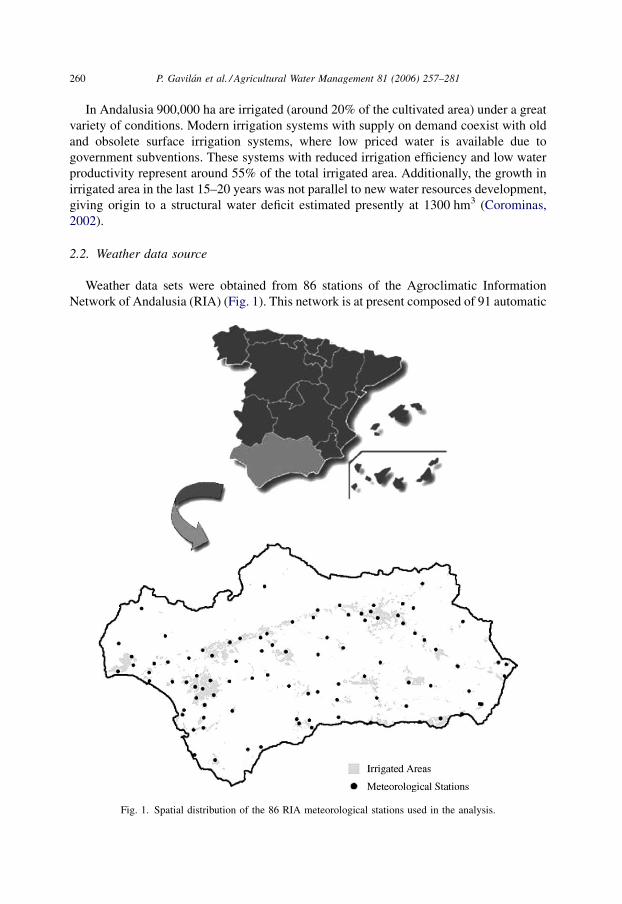
Weather data sets were obtained from 86 stations of the Agroclimatic Information

Network of Andalusia (RIA) (Fig. 1). This network is at present composed of 91 automatic

P. Gavilan et al. / Agricultural Water Management 81 (2006) 257–281260

Fig. 1. Spatial distribution of the 86 RIA meteorological stations used in the analysis.

weather stations, although only 86 of these were used in the present study. The other five

stations have been recently installed and their data series were too short. This network was

deployed to provide coverage to most of the irrigated area (De Haro et al., 2003). It was

designed and installed during 1999–2000 by the Ministry of Agriculture, Fisheries and

Food of Spain (MAPYA) to improve irrigation water management. Funding came from the

European Union. Network exploitation and maintenance are carried out by the IFAPA

(Agricultural Research Institute of Regional Government of Andalusia). Each station is

controlled by a CR10X datalogger (Campbell Scientific) and is equipped with sensors to

measure air temperature and relative humidity (HMP45A probe, Vaisala), solar radiation

(pyranometer SP1110 Skye), wind speed and direction (wind monitor RM Young 05103)

and rainfall (tipping bucket rain gauge ARG 100). Air temperature and relative humidity

are measured at 1.5 m and wind speed at 2 m above soil surface. Mean semi hourly and

daily average values are registered for each meteorological variable. Transfer of data from

stations to the data-collecting seat (Main Center) is accomplished by using GSM modems.

The Main Center incorporates a server, which sequentially connects to each station to

download the information collected during the last 24 h. Once the data from the stations are

downloaded, they are processed and transferred to a database. The Main Center is

responsible for quality control procedures that comprise the routine maintenance program

of the network, including sensor calibration and data validation. The collected values from

each station are checked for validity by different tests: range, step and persistence,

according to Meek and Hatfield (1994) and Shafer et al. (2000). Additionally, a specific test

has been performed for solar radiation measurements, according to Allen (1996).

Only daily averages were used for the study. At least two years of data per station were

used although for most of the stations (73 sites) three years were available and used.

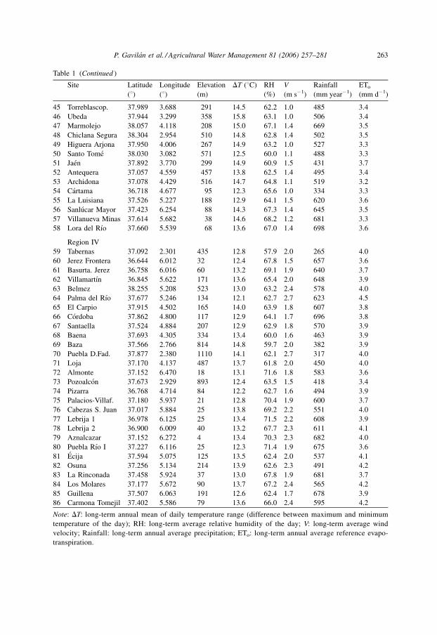
Locations of the 86 stations are given in Table 1 and Fig. 1. Site elevations ranged from 4 to

1212 m above mean sea level; longitude, from 184600900W to 781404900W; and latitude,

from 3681701000N to 3881801400N. In Table 1, the annual average values of meteorological

stations are reported. Average annual precipitation ranged from 183 to 804 mm; average

annual air temperature, from 12.9 to 18.9 8C; relative humidity, from 54 to 74%; and

annual average windspeed, from 0.9 to 3.1 m s�1. Fifteen sites can be considered as coastal

and 71 as inland locations. Therefore, the geographic and climatic diversity of the sites is

evident and representative of the Andalusian irrigation districts.

2.3. ET reference methods

The use of a standard method to develop or calibrate an equation for computing ETo is

necessary when measurements of ETo are not available. Advantages and disadvantages of

this procedure are described by Irmak et al. (2003). The use of one equation to calibrate or

validate another equation is not recent and many authors have used and recommended this

procedure (Allen et al., 1998; Itenfisu et al., 2003; Irmak et al., 2003). In addition, the FAO

Expert Consultation on Revision of FAO Methodologies for Crop Water Requirements

recommended that empirical methods should be calibrated or validated using the Penman–

Monteith equation as reference (Smith et al., 1991). This equation has proved to behave

well under a variety of climatic conditions, and that is the reason why it was decided to use

the FAO-56 Penman–Monteith (FAO-56 P–M) equation as reference to evaluate and

P. Gavilan et al. / Agricultural Water Management 81 (2006) 257–281 261

P. Gavilan et al. / Agricultural Water Management 81 (2006) 257–281262

Table 1

Summary of weather station site characteristics used in the study

Site Latitude

(8)Longitude

(8)Elevation

(m)

DT (8C) RH

(%)

V

(m s�1)

Rainfall

(mm year�1)

ETo

(mm d�1)

Region I

1 Cuevas Almanz. 37.258 1.799 20 10.2 64.5 1.1 201 3.3

2 Conil Frontera 36.337 6.131 26 11.0 73.3 1.3 411 3.3

3 Cadiar 36.924 3.182 950 10.6 57.7 1.3 507 3.3

4 Moguer Cebollar 37.241 6.801 63 11.8 69.1 1.4 443 3.4

5 Alcaudete 37.578 4.077 645 10.9 57.6 1.1 564 3.4

6 Malaga 36.757 4.536 68 11.1 63.3 1.2 492 3.5

7 Puebla Cazalla 37.219 5.349 229 12.0 61.3 1.4 582 3.7

Region II

8 La Mojonera 37.789 2.703 142 8.3 62.7 2.0 272 3.8

9 Almerıa 36.836 2.402 22 8.8 65.3 1.6 183 3.7

10 Nıjar 36.952 2.156 182 9.7 63.2 2.0 264 3.9

11 Finana 37.158 2.837 971 10.6 54.5 2.7 308 4.2

12 V. de Fatima 37.390 1.769 185 10.0 61.1 2.3 239 4.1

13 Tıjola 37.373 2.456 740 10.9 59.0 2.2 284 3.9

14 Adra 36.748 2.992 42 7.3 68.9 1.8 284 3.4

15 Sanlucar B. 36.835 6.294 22 11.8 73.1 2.4 544 3.8

16 Vejer Frontera 36.286 5.839 24 10.4 70.5 3.1 571 3.9

17 Jimena Frontera 36.414 5.384 53 11.7 69.9 2.2 795 3.7

18 Pto. Sta.Marıa 36.617 6.151 20 11.2 69.3 2.6 727 3.9

19 Hornachuelos 37.721 5.159 157 11.9 62.2 1.9 687 4.0

20 Iznalloz 37.417 3.550 935 11.6 58.1 2.1 651 3.8

21 Jerez Marq. 37.192 3.149 1212 11.9 56.4 1.8 381 3.5

22 Tojalillo-Gib. 37.319 7.018 52 11.6 66.9 2.1 692 4.0

23 Lepe 37.241 7.243 74 9.6 69.6 2.4 542 4.0

24 Gibraleon 37.414 7.059 169 10.8 66.6 1.8 724 3.8

25 Puebla Guzman 37.553 7.247 288 11.1 67.0 3.1 642 4.3

26 El Campillo 37.662 6.598 406 10.3 62.2 2.1 804 3.9

27 Palma Condado 37.386 6.540 192 11.1 65.0 1.9 664 3.8

28 S.Jose Propios 37.859 3.229 509 11.2 55.9 2.8 391 4.6

29 Sabiote 38.081 3.234 822 9.5 58.9 2.5 466 3.9

30 Mancha Real 37.917 3.595 436 11.7 56.9 2.0 434 4.0

31 Linares 38.06 3.648 443 11.3 57.9 2.0 484 4.0

32 Velez Malaga 36.797 4.130 49 11.9 63.7 1.7 457 3.9

33 Estepona 36.446 5.208 199 8.3 61.7 2.6 669 4.0

34 Sierra Yeguas 37.139 4.835 464 11.7 64.3 2.3 523 3.8

35 Churriana 36.675 4.502 32 10.2 64.5 2.1 432 3.9

36 Puebla Rıo II 37.081 6.045 41 11.7 71.9 1.8 563 3.7

Region III

37 Huercal-Overa 37.413 1.883 317 13.3 62.7 1.4 280 3.6

38 Adamuz 37.099 4.444 90 14.1 64.4 1.2 671 3.4

39 Pinos Puente 37.263 3.772 594 14.5 59.5 0.9 472 3.3

40 Zafarraya 36.841 4.152 905 12.5 66.1 1.3 684 3.1

41 Padul 37.020 3.599 781 12.8 59.1 1.2 444 3.4

42 Moguer 37.148 6.791 87 12.2 74.4 0.9 667 3.1

43 Niebla 37.348 6.734 52 13.2 69.3 1.5 702 3.6

44 Aroche 37.959 6.944 299 13.5 66.1 1.4 791 3.5

P. Gavilan et al. / Agricultural Water Management 81 (2006) 257–281 263

Table 1 (Continued )

Site Latitude

(8)Longitude

(8)Elevation

(m)

DT (8C) RH

(%)

V

(m s�1)

Rainfall

(mm year�1)

ETo

(mm d�1)

45 Torreblascop. 37.989 3.688 291 14.5 62.2 1.0 485 3.4

46 Ubeda 37.944 3.299 358 15.8 63.1 1.0 506 3.4

47 Marmolejo 38.057 4.118 208 15.0 67.1 1.4 669 3.5

48 Chiclana Segura 38.304 2.954 510 14.8 62.8 1.4 502 3.5

49 Higuera Arjona 37.950 4.006 267 14.9 63.2 1.0 527 3.3

50 Santo Tome 38.030 3.082 571 12.5 60.0 1.1 488 3.3

51 Jaen 37.892 3.770 299 14.9 60.9 1.5 431 3.7

52 Antequera 37.057 4.559 457 13.8 62.5 1.4 495 3.4

53 Archidona 37.078 4.429 516 14.7 64.8 1.1 519 3.2

54 Cartama 36.718 4.677 95 12.3 65.6 1.0 334 3.3

55 La Luisiana 37.526 5.227 188 12.9 64.1 1.5 620 3.6

56 Sanlucar Mayor 37.423 6.254 88 14.3 67.3 1.4 645 3.5

57 Villanueva Minas 37.614 5.682 38 14.6 68.2 1.2 681 3.3

58 Lora del Rıo 37.660 5.539 68 13.6 67.0 1.4 698 3.6

Region IV

59 Tabernas 37.092 2.301 435 12.8 57.9 2.0 265 4.0

60 Jerez Frontera 36.644 6.012 32 12.4 67.8 1.5 657 3.6

61 Basurta. Jerez 36.758 6.016 60 13.2 69.1 1.9 640 3.7

62 Villamartın 36.845 5.622 171 13.6 65.4 2.0 648 3.9

63 Belmez 38.255 5.208 523 13.0 63.2 2.4 578 4.0

64 Palma del Rıo 37.677 5.246 134 12.1 62.7 2.7 623 4.5

65 El Carpio 37.915 4.502 165 14.0 63.9 1.8 607 3.8

66 Cordoba 37.862 4.800 117 12.9 64.1 1.7 696 3.8

67 Santaella 37.524 4.884 207 12.9 62.9 1.8 570 3.9

68 Baena 37.693 4.305 334 13.4 60.0 1.6 463 3.9

69 Baza 37.566 2.766 814 14.8 59.7 2.0 382 3.9

70 Puebla D.Fad. 37.877 2.380 1110 14.1 62.1 2.7 317 4.0

71 Loja 37.170 4.137 487 13.7 61.8 2.0 450 4.0

72 Almonte 37.152 6.470 18 13.1 71.6 1.8 583 3.6

73 Pozoalcon 37.673 2.929 893 12.4 63.5 1.5 418 3.4

74 Pizarra 36.768 4.714 84 12.2 62.7 1.6 494 3.9

75 Palacios-Villaf. 37.180 5.937 21 12.8 70.4 1.9 600 3.7

76 Cabezas S. Juan 37.017 5.884 25 13.8 69.2 2.2 551 4.0

77 Lebrija 1 36.978 6.125 25 13.4 71.5 2.2 608 3.9

78 Lebrija 2 36.900 6.009 40 13.2 67.7 2.3 611 4.1

79 Aznalcazar 37.152 6.272 4 13.4 70.3 2.3 682 4.0

80 Puebla Rıo I 37.227 6.116 25 12.3 71.4 1.9 675 3.6

81 Ecija 37.594 5.075 125 13.5 62.4 2.0 537 4.1

82 Osuna 37.256 5.134 214 13.9 62.6 2.3 491 4.2

83 La Rinconada 37.458 5.924 37 13.0 67.8 1.9 681 3.7

84 Los Molares 37.177 5.672 90 13.7 67.2 2.4 565 4.2

85 Guillena 37.507 6.063 191 12.6 62.4 1.7 678 3.9

86 Carmona Tomejil 37.402 5.586 79 13.6 66.0 2.4 595 4.2

Note: DT: long-term annual mean of daily temperature range (difference between maximum and minimum

temperature of the day); RH: long-term average relative humidity of the day; V: long-term average wind

velocity; Rainfall: long-term annual average precipitation; ETo: long-term annual average reference evapo-

transpiration.

calibrate the Hargreaves equation in this work. That equation can be written as (Allen et al.,

1998):

EToPM ¼ 0:408DðRn � GÞ þ gð900=ðT þ 273ÞÞu2ðes � eaÞDþ gð1 þ 0:34u2Þ

(1)

where ETo is the computed reference evapotranspiration (mm d�1); D is the slope of

saturation vapor pressure versus air temperature curve (kPa 8C�1); Rn is the daily net

radiation (MJ m�2 d�1); G is the soil heat flux (MJ m�2 d�1); g is the psychrometric

constant (kPa 8C�1); T is the mean air temperature at 2 m height (8C); u2 is the daily mean

of wind speed at 2 m height (m s�1); es is the saturation vapor pressure (kPa); and ea is the

actual vapor pressure (kPa). All parameters were calculated using the equations provided

by Allen et al. (1998). The soil heat flux (G) was assumed to be zero over the calculation

time step period (24 h).

The Hargreaves equation (Hargreaves and Samani, 1985) can be written as:

EToH ¼ 0:0023RaðT þ 17:8ÞffiffiffiffiffiffiffiffiffiffiffiffiffiffiffiffiffiffiffiffiffiffiffiTmax � Tmin

p(2)

where ETo is the computed reference evapotranspiration (mm d�1); Ra is the water

equivalent of the extraterrestrial radiation (mm d�1) computed according to Allen et al.

(1998); Tmax, Tmin and T are the daily maximum, minimum and mean air temperature (8C),

with T calculated as the average of Tmax and Tmin. 0.0023 is the original empirical

coefficient proposed by Hargreaves and Samani (1985).

2.4. Validation

Although the correction proposed in this work is based on regional calibration, with data

covering a diversity of climatic conditions (from subtropical coastal areas in the southeast

to semi-desert areas in the east), it is advisable to validate it. The proposed adjustment was

validated by using data from 14 meteorological stations located in different areas of Spain

and belonging to the Agroclimatic Information System (SIAR) from Ministry of

Agriculture, Fisheries and Food (MAPYA). Site elevations ranged from 6 to 717 m above

mean sea level; longitude, from 080802400W to 585600400W; and latitude, from 3783603600Nto 4181004800N. Average annual precipitation ranged from 144 to 892 mm; average annual

air temperature, from 11.3 to 18.6 8C; relative humidity, from 58 to 72%; and annual

average windspeed, from 1.2 to 2.6 m s�1. Two sites can be considered as coastal and 12 as

inland locations. Three years of measured daily weather data were used in the validation

process (from 2001 to 2003). The EToPM method was also used as reference for

comparison.

2.5. Statistical analysis

ETo estimates from both methods were compared by using simple error analysis and

linear regression. For each location, the following parameters were calculated (Willmott,

1982): mean bias error (MBE), root mean square error (RMSE), relative error (RE) and the

ratio between both average ETo estimations (R). Additionally, maximum, minimum, mean

P. Gavilan et al. / Agricultural Water Management 81 (2006) 257–281264

and standard deviations of RMSE, MBE and R for each different group of locations

(Itenfisu et al., 2003) were also calculated.

MBE ¼Pn

i¼1ðyi � xiÞn

(3)

RMSE ¼

ffiffiffiffiffiffiffiffiffiffiffiffiffiffiffiffiffiffiffiffiffiffiffiffiffiffiffiffiffiPni¼1ðyi � xiÞ2

n

s(4)

RE ¼ MBE

x� 100 (5)

R ¼ yave

xave

(6)

where n is the number of available days; yi is the estimated EToH; xi is the estimated EToPM;

xave and yave are the averages of EToPM and EToH for a given site, respectively.

3. Results

3.1. Penman–Monteith FAO-56 versus Hargreaves ETo

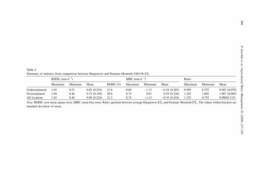
Variability from one location to another in the results of comparison between both

methods was clearly apparent. Thirty five locations significantly underestimated daily ETo

with respect to Penman–Monteith FAO-56 ETo and 21 clearly overestimated it. The

method provided satisfactorily good ETo estimations for 30 locations (under- or

overestimations were smaller than 5%). Considering all locations, the MBE values ranged

from 0.74 to �1.13 mm d�1, with a mean of �0.10 mm d�1 (Table 2). RMSE ranged from

0.46 to 1.65 mm d�1, with an average value of 0.80 mm d�1. Ratios between EToH and

EToPM mean values showed that maximum underestimation produced was as high as 24.5%

and the maximum overestimation found amounted to 22.5%. Considering only locations

where Hargreaves equation underestimated ETo, the MBE reached a minimum of

�1.13 mm d�1, with a mean value of �0.38 mm d�1. In this case, RMSE ranged from 0.51

to 1.65 mm d�1, with an average value of 0.85 mm d�1. The ETo ratio, as defined above,

was 0.903 indicating a mean underestimation of 10% derived from the use of Hargreaves

equation. In locations where Hargreaves equation overestimated ETo, the mean value of

MBE was equal to 0.29 mm d�1, ranging from 0.01 to 0.74 mm d�1, whereas RMSE

varied between 0.46 and 1.04 mm d�1, with an average value of 0.72 mm d�1. In the latter

case, R was 1.087, indicating a mean overestimation of 9%.

The greatest underestimations occurred mainly for stations located in coastal areas,

although there were some inland stations showing the same tendency. In all cases, high

windspeed and small DT values were found. By contrast, the greatest overestimations took

place at inland areas with high DT values and low windspeeds, although some

overestimations were also present near the coast. Therefore, the method was more accurate

for windy locations with high DT values, and for non windy sites with low or moderate DT

values. It can be concluded that the lack of agreement between both methods were not only

P. Gavilan et al. / Agricultural Water Management 81 (2006) 257–281 265

P.

Ga

vilan

eta

l./Ag

ricultu

ral

Wa

terM

an

ag

emen

t8

1(2

00

6)

25

7–

28

12

66

Table 2

Summary of statistics from comparison between Hargreaves and Penman–Monteith FAO-56 ETo

RMSE (mm d�1) MBE (mm d�1) Ratio

Maximum Minimum Mean RMSE (%) Maximum Minimum Mean Maximum Minimum Mean

Underestimated 1.65 0.51 0.85 (0.254) 21.8 0.00 �1.13 �0.38 (0.285) 0.999 0.755 0.903 (0.070)

Overestimated 1.04 0.46 0.72 (0.149) 20.6 0.74 0.01 0.29 (0.226) 1.225 1.002 1.087 (0.069)

All locations 1.65 0.46 0.80 (0.224) 21.2 0.74 �1.13 �0.10 (0.424) 1.225 0.755 0.980(0.115)

Note: RMSE: root mean square error. MBE: mean bias error. Ratio: quotient between average Hargreaves ETo and Penman–Monteith ETo. The values within brackets are

standard deviation of mean.

affected by the geographical locations of the stations, but also, and mainly, by climatic

conditions.

Fifteen stations are located close to the coast. High underestimations occurred at 12 of

them, where MBE reached a minimum of �0.97 mm d�1, with a mean value of

�0.62 mm d�1. For two of them, the performance of the equation was good and only for

one there was a clear overestimation, with a MBE of 0.40 mm d�1. Annual mean value of

DT at coastal locations was 10 8C. Underestimations increased as the annual average DT

decreased. Therefore, as a first approximation, it may be inferred that when the annual DT

value is small, ETo tends to be underestimated as a consequence of the underestimation of

Rs by the Hargreaves equation.

At most of the inland stations, annual average of daily DT values was higher than 11 8C,

with an average of 12.8 8C. Locations with high DT values tended to overestimate ETo,

although variability observed under these conditions suggested that other factors could

affect the accuracy of the method, indicating that an adjustment based only on DT could be

insufficient. Furthermore, a certain correlation was found between annual average

windspeed and the accuracy of the method, with errors being greater for higher windspeed,

especially above 2 m s�1, when underestimations were more clear.

Inability of the Hargreaves equation to account for the effects of high windspeeds as

well as for high vapor pressure deficits (typical advective conditions in semiarid

environments) has been established (Martınez-Cob and Tejero-Juste, 2004; Berengena

and Gavilan, 2005; Temesgen et al., 2005). Thus, an adjustment including this new

variable would be more adequate, as these authors proposed. Although corrections based

on wind functions are not practical, because windspeed records are only available from

no more than a few weather stations, a calibration based on a qualitative knowledge of

windspeed conditions at the site could be enough (Martınez-Cob and Tejero-Juste,

2004).

A detailed analysis has been undertaken representing every station in a coordinate

system as a point defined by their respective annual DT and V mean values. For

convenience, four regions were delimited in the graph defined by DT = 12 8C and

V = 1.5 m s�1 (see Fig. 2). In the first region (DT < 12 8C and V < 1.5 m s�1) some coastal

stations and three inland locations were found, with annual mean windspeeds ranging from

1.1 to 1.4 m s�1 and MBE less than 0.11 mm d�1 (Table 3). Within the second region

(DT < 12 8C and V > 1.5 m s�1), the method usually underestimated as a result of the

increase in the aerodynamic component of the evapotranspiration, which is not accounted

for by the Hargreaves equation. In this case, the minimum MBE was �1.13 mm d�1 and

the maximum RMSE, 1.65 mm d�1. For the stations located in the third region

(DT > 12 8C and V < 1.5 m s�1) Hargreaves equation overestimated ETo, due to high DT

values, with an average overestimation of 0.43 mm d�1, which is the average value of the

MBE, and a maximum RMSE of 1.04 mm d�1. And finally, within the fourth region

(DT > 12 8C and V > 1.5 m s�1), the relatively high windspeeds tended to produce

underestimations, but this tendency was partially compensated by the opposite effect

produced by high values of DT, so that the MBE for this region was less than

�0.37 mm d�1, with only two exceptions in which average windspeed was very high

(higher than 2.7 m s�1). As it will be seen, in these cases – very high windspeed and high

DT – a specific correction should be applied. It can be thus concluded that, in our

P. Gavilan et al. / Agricultural Water Management 81 (2006) 257–281 267

conditions, stations located in regions I and IV do not require adjustment, whereas those

located in regions II and III should be adjusted to obtain more accurate estimates.

3.2. Adjusted coefficients

Forcing regressions lines – EToH on EToPM – through the origin, the ratio between

0.0023 and the regression slope would provide a locally adjusted coefficient of the

Hargreaves equation for each location (Fig. 3). For stations located in regions I and IV,

mean values of those new coefficients were close to 0.0023, they were 0.00235 and

0.00241, respectively, with deviations amounting to 2 and 5% over the original value. For

the latter case, the average of the adjusted coefficients rose so much due to the existence of

two stations in which the windspeed was especially high. For these, the adjusted

coefficients increased up to 0.0029. For region II the average value for the new coefficients

was 0.00273, which is about 19% higher than the original value, while for region III

became about 9% smaller (0.00209). So, it was proposed to use new coefficients equals to

0.0027 and 0.0021, instead of 0.0023, for stations located in regions II and III, respectively.

Stations located in regions I and IV should not require adjustment, although under high

wind conditions it may be advisable to increase up to 0.0026 the value of the coefficient for

stations located in region IV. This last coefficient is not taken into consideration in the

discussion that follows.

Corrected Hargreaves ETo values can then be easily obtained by knowing DT and

windspeed. The first variable is readily available for most locations, but this is not usually

the case for windspeed. However, a qualitative knowledge of windspeed conditions at the

P. Gavilan et al. / Agricultural Water Management 81 (2006) 257–281268

Fig. 2. Distribution of each location in function of annual means of windspeed (V) and annual mean of daily

temperature range (DT).

P.

Ga

vilan

eta

l./Ag

ricultu

ral

Wa

terM

an

ag

emen

t8

1(2

00

6)

25

7–

28

12

69

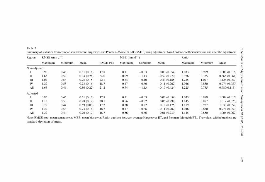
Table 3

Summary of statistics from comparison between Hargreaves and Penman–Monteith FAO-56 ETo using adjustment based on two coefficients before and after the adjustment

Region RMSE (mm d�1) MBE (mm d�1) Ratio

Maximum Minimum Mean RMSE (%) Maximum Minimum Mean Maximum Minimum Mean

Non-adjusted

I 0.96 0.46 0.61 (0.16) 17.8 0.11 �0.03 0.03 (0.054) 1.033 0.989 1.008 (0.016)

II 1.65 0.52 0.94 (0.26) 24.0 �0.09 �1.13 �0.52 (0.270) 0.976 0.755 0.866 (0.064)

III 1.04 0.56 0.75 (0.15) 22.1 0.74 0.10 0.43 (0.185) 1.225 1.027 1.128 (0.057)

IV 1.22 0.53 0.73 (0.16) 18.7 0.17 �0.66 �0.11 (0.202) 1.046 0.850 0.974 (0.050)

All 1.65 0.46 0.80 (0.22) 21.2 0.74 �1.13 �0.10 (0.424) 1.225 0.755 0.980(0.115)

Adjusted

I 0.96 0.46 0.61 (0.16) 17.8 0.11 �0.03 0.03 (0.054) 1.033 0.989 1.008 (0.016)

II 1.13 0.53 0.78 (0.17) 20.1 0.56 �0.52 0.05 (0.298) 1.145 0.887 1.017 (0.075)

III 0.79 0.44 0.59 (0.09) 17.2 0.38 �0.22 0.10 (0.175) 1.119 0.937 1.030 (0.052)

IV 1.22 0.53 0.73 (0.16) 18.7 0.17 �0.66 �0.11 (0.202) 1.046 0.850 0.974 (0.050)

All 1.22 0.44 0.70 (0.17) 18.7 0.56 �0.66 0.01 (0.239) 1.145 0.850 1.006 (0.062)

Note: RMSE: root mean square error. MBE: mean bias error. Ratio: quotient between average Hargreaves ETo and Penman–Monteith ETo. The values within brackets are

standard deviation of mean.

site will suffice, and the correction procedure will only require deciding whether the

location is windy or not, as Martınez-Cob and Tejero-Juste (2004) proposed. For this

purpose, these authors proposed using some indirect assessment of windspeed based on

such characteristics as topography of the area and presence of wind mills for wind power

energy production, besides any other data furnished by the national meteorological

institutions.

The use of two new coefficients improved prediction over the original Hargreaves

equation. After adjustment, the maximum MBE for locations in region II was reduced from

�1.13 to �0.52 mm d�1, which resulted in an improvement of 54% (Table 3 and Fig. 4).

The average increase in accuracy, quantified by the decrease of RMSE, was 17% (from

0.94 to 0.78 mm d�1). Maximum RMSE decreased from 1.65 to 1.13 mm d�1, which

resulted in an improvement of 31% (Fig. 5). Average RMSE in region III decreased by 21%

(from 0.75 to 0.59 mm d�1) and maximum MBE decreased from 0.74 to 0.38 mm d�1

(49% improvement). Considering all locations, the average RMSE was 0.70 mm d�1, an

average increase in accuracy of 12% with respect to the initial value. Finally, maximum and

minimum MBE were 0.56 and �0.66 mm d�1, which meant an improvement of 24 and

41%, respectively. After adjustment, standard deviation of RMSE and MBE decreased 25

and 44%, respectively, indicating the gain in uniformity. Adjustment was not applied to

eliminate high underestimations that occurred at the region IV stations, which were

affected by average windspeed above 2.5 m s�1. Here, it would be necessary to use a third

coefficient (0.0026) for strong-wind locations in that region, as previously stated. The

P. Gavilan et al. / Agricultural Water Management 81 (2006) 257–281270

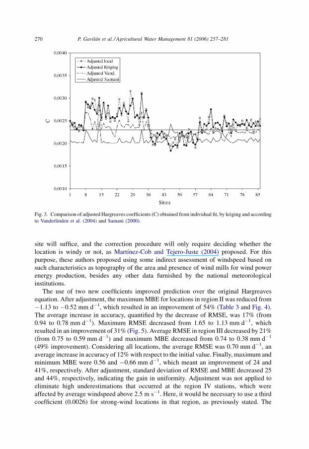
Fig. 3. Comparison of adjusted Hargreaves coefficients (C) obtained from individual fit, by kriging and according

to Vanderlinden et al. (2004) and Samani (2000).

P. Gavilan et al. / Agricultural Water Management 81 (2006) 257–281 271

Fig. 4. Comparison of unadjusted and adjusted MBE values using method based on two coefficients.

Fig. 5. Comparison of unadjusted and adjusted RMSE values using method based on two coefficients.

proposed correction improved accuracy for 43 out of the 51 locations included in the

regions affected by the adjustment (II and III). The other eight stations for which the new

coefficient did not improve the equation performance were located close to the region

borders (Fig. 2). For regions I and IV, not affected by the adjustment, 31 locations showed

quite accurate estimates, and the results were not satisfactory in only four cases. It can be

concluded that after the adjustment, 74 out of the 86 locations studied gave quite accurate

results, with relative values of MBE lower than 10% in most cases.

The use of only two adjustment coefficients, as described above, limits to a certain

degree the correction procedure. To get a more accurate adjustment, the kriging method

was applied to obtain adjusted coefficients based on DT and windspeed. Windspeed and DT

were used as independent variables, while the locally adjusted empirical coefficient was

taken as the dependent variable. Afterwards, new adjusted coefficients, functions of DT for

three windspeed conditions (low, moderate and high), were obtained by using linear

regression (Eqs. (7)–(9)):

Cadj ¼ �0:000117DT þ 0:003689 ðlowÞ (7)

Cadj ¼ �0:000098DT þ 0:003723 ðmoderateÞ (8)

Cadj ¼ �0:000087DT þ 0:003810 ðhighÞ (9)

Adopted limits from low to moderate and from moderate to high windspeed were 1.5

and 2.5 m s�1, respectively.

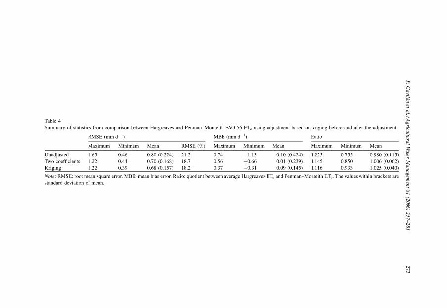
After the kriging adjustment, the average RMSE was reduced to 0.68 mm d�1, which

meant an improvement of 15% of the initial value (Table 4). Maximum and minimum

RMSE values were 1.22 and 0.39 mm d�1 (Fig. 6), which represented a reduction of 26 and

16%, respectively (Table 5). Standard deviation for RMSE was reduced 30%, indicating

the uniformity of the improvement. Maximum and minimum MBE were 0.37 and

�0.31 mm d�1, which was equivalent to a reduction of 50 and 70%, respectively (Fig. 7).

Comparing these values with the results of the adjustment based on two fixed coefficients,

an increase in accuracy of 5% for the average RMSE and of 26 and 25% for maximum and

minimum values of MBE, respectively, was obtained, which certainly justified preference

for this latter adjustment. Besides, after the adjustment, standard deviations for RMSE and

MBE were reduced by 30 and 66%, respectively, indicating that the correction was more

generalized. However, it should be noted that, after correction, some bias still remained in

the estimates. In fact, as can be seen in Fig. 7, a slight tendency to overestimate ETo at most

locations remained after adjustment, although in all cases MBE was smaller than

0.37 mm d�1 (representing 10% error on the average ETo) and at 70% of them, the error

was less than 5% of the average ETo. Adjustment improved accuracy at 65 locations.

Nevertheless, behavior was poor for region IV, as in most locations of this region

adjustment worsened results. Therefore, except at very windy locations, where the

adjustment was very good, it would be preferable not to apply the correction, considering

original results quite accurate.

P. Gavilan et al. / Agricultural Water Management 81 (2006) 257–281272

P.

Ga

vilan

eta

l./Ag

ricultu

ral

Wa

terM

an

ag

emen

t8

1(2

00

6)

25

7–

28

12

73

Table 4

Summary of statistics from comparison between Hargreaves and Penman–Monteith FAO-56 ETo using adjustment based on kriging before and after the adjustment

RMSE (mm d�1) MBE (mm d�1) Ratio

Maximum Minimum Mean RMSE (%) Maximum Minimum Mean Maximum Minimum Mean

Unadjusted 1.65 0.46 0.80 (0.224) 21.2 0.74 �1.13 �0.10 (0.424) 1.225 0.755 0.980 (0.115)

Two coefficients 1.22 0.44 0.70 (0.168) 18.7 0.56 �0.66 0.01 (0.239) 1.145 0.850 1.006 (0.062)

Kriging 1.22 0.39 0.68 (0.157) 18.2 0.37 �0.31 0.09 (0.145) 1.116 0.933 1.025 (0.040)

Note: RMSE: root mean square error. MBE: mean bias error. Ratio: quotient between average Hargreaves ETo and Penman–Monteith ETo. The values within brackets are

standard deviation of mean.

3.3. Comparison of alternative corrections

Most recent correction procedures for Hargreaves equation were proposed by Samani

(2000) and Vanderlinden et al. (2004). Both improvements are based only on the use of an

adjusted temperature dependent coefficient and were developed in USA and Southern

Spain, respectively. Fig. 3 compares the adjusted coefficients obtained from individual fit

using Eqs. (7)–(9), against those calculated according to approaches of Samani (2000) and

Vanderlinden et al. (2004). The horizontal line represents the original coefficient of

Hargreaves (0.0023). Values adjusted by Samani were generally smaller than 0.0023 and

produced underestimations in most instances. In this case, adjustment was not sufficient

because the Samani approach was developed using data from a greater variety of climates

throughout the USA. The approach of Vanderlinden et al. (2004) performed better,

although their correction was not sufficient to compensate underestimations at locations

included within region II and overestimations for region III. For developing their approach,

these authors used estimated, from bright sunshine hour, rather than measured solar

radiation values. These could have led to an underestimation of that variable (Gavilan,

nonpublished data), affecting the soundness of the approach.

3.4. Validation

Only kriging adjustment was subject to validation, as this method was considered more

global and accurate than that based on four regions in the DT and V domains (two fixed

coefficients). After the adjustment, average RMSE was reduced to 0.73 mm d�1, which

P. Gavilan et al. / Agricultural Water Management 81 (2006) 257–281274

Fig. 6. Comparison of unadjusted and adjusted RMSE values using method based on kriging.

P.

Ga

vilan

eta

l./Ag

ricultu

ral

Wa

terM

an

ag

emen

t8

1(2

00

6)

25

7–

28

12

75

Table 5

Improvement (%) obtained of applying adjustment based on two coefficients and kriging methods

RMSE MBE Ratio

Maximum Minimum Mean RMSE (%) Maximum Minimum Mean Maximum Minimum Mean

Two coefficients 26 6 12 (25) 12 24 41 90 (44) 7 12 3 (46)

Kriging 26 16 15 (30) 14 50 73 10 (66) 11 18 �4.6 (65.4)

Note: RMSE: root mean square error. MBE: mean bias error. Ratio: quotient between average Hargreaves ETo and Penman–Monteith ETo. The values within brackets are

standard deviation of mean.

represented a decrease of 7% (Table 6). Maximum and minimum RMSE values were 1.04

and 0.47 mm d�1, which represented a reduction of 5 and 11%, respectively. Standard

deviation of RMSE was reduced 10%. Maximum and minimum MBE were 0.33 and

�0.36 mm d�1, equivalent to a reduction of 51 and 55%, respectively. Finally, standard

deviations for RMSE and MBE were reduced 10 and 50%, respectively, indicating that

adjustment was generalized. The correction was adequate at 10 locations, especially at 7

sites. However, the adjustment worsened the original estimates at 4 locations (Fig. 8).

These poor results occurred again for stations located at region IV with windspeed lower

than 2 m s�1 (locations 9, 10 and 11). Again, it is advisable not to apply adjustment to these

stations, unless they were very windy locations (locations 7, 8, 12 and 13). Considering all

locations, adjustment limited the errors to 10% of average ETo and the errors were lower

than 5% at 6 of them.

3.5. Agronomic consequences

The Hargreaves equation has been frequently used to calculate crop water requirements

and for irrigation scheduling under semiarid conditions in the Guadalquivir valley in

Southern Spain (Pastor et al., 1999) and other regions in the world (Di Stefano and Ferro,

1997; Beyazgul et al., 2000). The equation allows more accurate calculations of crop water

requirements using locally adjusted coefficients. To illustrate this, real data from

Villafranca Irrigation District (VID) in the mid Guadalquivir Valley near Cordoba were

used. Using Penman–Monteith equation throughout the years 2001–2003 at the closest

station (weather station #38, Adamuz; Table 1), average yearly accumulated ETo was

P. Gavilan et al. / Agricultural Water Management 81 (2006) 257–281276

Fig. 7. Comparison of unadjusted and adjusted MBE values using method based on kriging.

P.

Ga

vilan

eta

l./Ag

ricultu

ral

Wa

terM

an

ag

emen

t8

1(2

00

6)

25

7–

28

12

77

Table 6

Summary of statistics from comparison between Hargreaves and Penman–Monteith FAO-56 ETo using adjustment based on kriging before and after the adjustment at

stations located in other regions of Spain

RMSE (mm d�1) MBE (mm d�1) Ratio

Maximum Minimum Mean RMSE (%) Maximum Minimum Mean Maximum Minimum Mean

Unadjusted 1.10 0.53 0.78 (0.18) 23.0 0.67 �0.82 �0.10 (0.38) 1.24 0.78 0.977 (0.11)

Adjusted 1.04 0.47 0.73 (0.16) 21.3 0.33 �0.36 0.13 (0.19) 1.12 0.90 1.039 (0.06)

Note: RMSE: root mean square error, MBE: mean bias error. Ratio: quotient between average Hargreaves ETo and Penman–Monteith ETo. The values within brackets are

the standard deviation of mean).

P. Gavilan et al. / Agricultural Water Management 81 (2006) 257–281278

Fig. 8. Comparison of unadjusted and adjusted MBE values using method based on kriging at stations located in

other regions of Spain.

Fig. 9. Daily ETo estimates (monthly averaged) by Penman–Monteith FAO-56, Hargreaves and adjusted

Hargreaves equations at a representative location in the Guadalquivir Valley.

1232 mm (Fig. 9). Using Hargreaves equation, this figure was equal to 1451 mm, 17.8%

higher. This difference is more significant considering that 75% of the errors occurred

during irrigation season. For this period, from April to September, the accumulated ETo

was 929 and 1095 mm for Penman–Monteith and Hargreaves equations, respectively.

Corrected Hargreaves equation yielded 1287 and 971 mm, for the whole year and irrigation

season, respectively. Therefore, the adjusted Hargreaves equation overestimated the

accumulated ETo by only 4.5%, which is quite reasonable if we consider the uncertain

levels associated to other variables affecting the irrigation water use (principally crop

coefficient and system efficiency). In VID, the main crops are maize, cotton, sugar beet and

garlic. For these crops, using local crops coefficients (Lorite et al., 2004, adapted from

Allen et al., 1998), crop water requirements (ETr) were calculated for the whole growing

season. Water saving resulting from the use of corrected Hargreaves equation, ranged from

109 mm per year for cotton to 60 mm per year for garlic. Considering the whole irrigation

district, the water consumption will be affected depending on ETo estimation method.

Thus, consumption for VID was reduced by 11% using locally calibrated Hargreaves

equation instead of the original equation. These results show the importance of adjusting

empirical equations, such as the Hargreaves in the present case which affects yield and

waterlogging.

4. Conclusions

Results obtained from the comparisons of ETo daily estimates by Hargreaves equation

against Penman–Monteith FAO-56 – taken as standard – throughout the Andalusian region

(Southern Spain), showed a high spatial variability. At coastal areas, the Hargreaves

equation generally underpredicted ETo, although at some specific locations it was more

accurate, even overestimating in some cases. Behavior of the equation was less predictable

at inland areas, ranging from moderate underestimation to high overestimations.

Yearly means of windspeed (V) and daily temperature range (DT) appeared to affect the

accuracy of the equation. According to the values taken by those climatic variables, an

adjustment was proposed for some cases, consisting in the adoption of a different value for

the empirical coefficient; thus, the original coefficient (0.0023) should be replaced by

0.0021 when DT > 12 8C and V < 1.5 m s�1, and by 0.0027 when DT < 12 8C and

V > 1.5 m s�1. For all other cases, correction was not necessary. These locally adjusted

coefficients produced an important improvement in the equation performance.

An alternative method for adjustment based on kriging interpolation has been also

proposed and tested, yielding even better results. In this case, coefficients were not constant

for a group of stations as before, but they were individually obtained for each location as a

function of DT and V. This method was validated with data from other Spanish regions.

The adjustment based on kriging has proved more efficient, except at locations with

high DT and moderate windspeed. Under these conditions, a fixed value of 0.0026 is

suggested, but, as a general rule, it is recommended to calculate the coefficient by this

procedure for the rest of the cases.

The practical consequences of the proposed adjustment were made evident with data

from an irrigation district in the Guadalquivir valley. Using local crop coefficients for the

P. Gavilan et al. / Agricultural Water Management 81 (2006) 257–281 279

most important crops in the area, water consumption was reduced by 11% if the corrected

equation were used instead of the original one.

It should be taken into account that this study was based on the analysis of a limited data

set, with series never longer than 3 years. Given the year to year variability of climatic

variables, a more comprehensive study, including longer series of data (10 years or more),

is advisable to improve the reliability of the proposed adjustments.

Acknowledgments

The authors are grateful to two anonymous reviewers for their valuable comments and

suggestions. Furthermore, they thank Mr. Juan de Haro for his valuable work in the

Agroclimatic Information System of Andalusia.

References

Allen, R.G., 1986. A Penman for all Seasons. J. Irrig. Drain. Eng. ASCE 111 (4), 348–368.

Allen R.G. 1993. Evaluation of a temperature difference method for computing grass reference evapotranspira-

tion. Report submitted to the Water Resources Development and Man Service, Land and Water Development

Division, FAO, Rome. 49 pp.

Allen, R.G., 1995. Evaluation of procedure for estimating mean monthly solar radiation from air temperature.

Report, United Nations Food and Agricultural Organization (FAO), Rome.

Allen, R.G., 1996. Assessing integrity of weather data for reference evapotranspiration estimation. J. Irrig. Drain.

Eng. ASCE 122 (2), 97–106.

Allen, R.G., Pereira, L.S., Raes, D., Smith, M., 1998. Crop evapotranspiration: Guidelines for computing crop

water requirements. FAO Irrigation and Drainage Paper no. 56, Rome.

Berengena, J., Gavilan, P., 2005. Reference evapotranspiration estimation in a highly advective semiarid

environment. J. Irrig. Drain. Eng. ASCE 131 (2), 147–163.

Beyazgul, M., Kayam, Y., Engelsman, F., 2000. Estimation methods for crop water requirements in the Gediz

Basin of western Turkey. J. Hydrol. 229, 19–26.

Corominas, J., 2002. Hacia una nueva polıtica de aguas en Andalucıa. III Congreso Iberico sobre Gestion y

Planificacion de Aguas. Sevilla, 13–17 de noviembre de 2002 (in Spanish).

De Haro, J.M., Gavilan, P., Fernandez, R., 2003. The Agroclimatic Information Network of Andalucıa. In:

Proceeding of the Third International Conference on Experiences with Automatic Weather Stations,

Torremolinos, Spain. 19–21, February..

Di Stefano, C., Ferro, V., 1997. Estimation of evapotranspiration by Hargreaves formula and remotely sensed data

in semiarid Mediterranean areas. J. Agric. Eng. Res. 68, 189–199.

Droogers, P., Allen, R.G., 2002. Estimating reference evapotranspiration under inaccurate data conditions. Irrig.

Drain. Syst. 16, 33–45.

Hargreaves, G.H., Samani, Z.A., 1982. Estimating potential evapotranspiration. J. Irrig. Drain. Eng. ASCE 108

(3), 223–230.

Hargreaves, G.H., Samani, Z.A., 1985. Reference crop evapotranspiration from temperature. Appl. Eng. Agric. 1

(2), 96–99.

Hargreaves, G.L., Hargreaves, G.H., Riley, J.P., 1985. Agricultural benefits for Senegal River basin. J. Irrig. Drain.

Eng. ASCE 111 (2), 113–124.

Hargreaves, G.H., Allen, R.G., 2003. History and evaluation of Hargreaves evapotranspiration equation. J. Irrig.

Drain. Eng. ASCE 129 (1), 53–63.

Heerman, D.F. 1986. Evapotranspiration Research Priorities for the Netx Decade-Irrigation. ASAE Paper no. 86–

2626. St. Joseph Mich. ASAE.

P. Gavilan et al. / Agricultural Water Management 81 (2006) 257–281280

Irmak, S., Irmak, A., Allen, R.G., Jones, J.W., 2003. Solar and net radiation-based equations to estimate reference

evapotranspiration in humid climates. J. Irrig. Drain. Eng. ASCE 129 (5), 336–347.

Itenfisu, D., Elliott, R.L., Allen, R.G., Walter, I.A., 2003. Comparison of reference evapotranspiration calculation

as part of the ASCE standardization effort. J. Irrig. Drain. Eng. ASCE 129 (6), 440–448.

Jensen, M.E., Burman, R.D., Allen, R.G. (Eds.), 1990. Evapotranspiration and Irrigation Water Requirements.

Committee on Irrigation Water Requirements of the Irrigation and Drainage Division of ASCE, New York.

Jensen, D.T., Hargreaves, G.H., Temesgen, B., Allen, R.G., 1997. Computation of ETo under non ideal conditions.

J. Irrig. Drain. Eng. ASCE 123 (5), 394–400.

Lorite, I.J., Mateos, L., Fereres, E., 2004. Evaluating irrigation performance in a Mediterranean environment. I

Model and general assessment of an irrigation scheme. Irrig. Sci. 23, 77–84.

Martınez-Cob, A., Tejero-Juste, M., 2004. A wind-based qualitative calibration of the Hargreaves ETo estimation

equation in semiarid regions. Agric. Water Manage. 64, 251–264.

Meek, D.W., Hatfield, J.L., 1994. Data quality checking for single station meteorological databases. Agric. For.

Meteorol. 69, 85–109.

Pastor, M., Castro, J., Mariscal, M.J., Vega, V., Orgaz, F., Fereres, E., Hidalgo, J., 1999. Respuestas del olivar

tradicional a diferentes estrategias and dosis de agua de riego. Investigacion Agraria: Produccion Vegetal 14

(3), 393–404 (in Spanish).

Pruitt, W.O., Doorenbos, J., 1977. Empirical Calibration, a Requisite for Evapotranspiration Formulae Based on

Daily or Longer Mean Climatic Data. Presented at International Round table Conference on Evapotranspira-

tion. International Commission on Irrigation and Drainage, Budapest, Hungary, 20 pp.

Samani, Z., 2000. Estimating solar radiation and evapotranspiration using minimum climatological data. J. Irrig.

Drain. Eng. ASCE 126 (4), 265–267.

Samani, Z., 2004. Discussion of ‘‘History and evaluation of Hargreaves evapotranspiration equation’’. J. Irrig.

Drain. Eng. ASCE 130 (5), 447–448.

Shafer, M.A., Fiebrich, C.A., Arndt, D.S., 2000. Quality assurance procedures in the Oklahoma Mesonetwork. J.

Atmos. Oceanic Technol. AMS 17, 474–494.

Sharma, M.L., 1985. Estimating evapotranspiration. In: Hillel, D. (Ed.), Advances in Irrigation, vol. 3. Academic

Press, London.

Smith, M., Allen, R.G., Monteith, J.L., Pereira, L.S., Perrier, A., Pruitt, W.O., 1991. Report on the expert

consultation on procedures for revision of FAO guidelines for prediction of crop water requirements. Land and

Water Development Division, United Nations Food and Agriculture Service, Rome.

Temesgen, B., Eching, S., Davidoff, B., Frame, K., 2005. Comparison of some reference evapotranspiration

equations for California. J. Irrig. Drain. Eng. ASCE 131 (1), 73–84.

Vanderlinden, K., Giraldez, J.V., Van Mervenne, M., 2004. Assessing reference evapotranspiration by the

Hargreaves method in Southern Spain. J. Irrig. Drain. Eng. ASCE 129 (1), 53–63.

Willmott, C.J., 1982. Some Comments on the Evaluation of Model Performance. Bull. Am. Meteorol. Soc. AMS

63 (11), 1309–1313.

Xu, C.Y., Singh, V.P., 2002. Cross comparison of empirical equations for calculating potential evapotranspiration

with data from Switzerland. Water Resour. Manage. 16, 197–219.

P. Gavilan et al. / Agricultural Water Management 81 (2006) 257–281 281